1
TICAM REPORT 96-10
February 1996
TUF 2.5 User Manual
Philip T. Keenan
TUF 2.5 User Manual1
Philip T. Keena.n2
February 6, 1996
IThis research was supported in part by the Department of Energy, the State of Texas Governor's Energy
Office, and project grants from the National Science Foundation. The author was also supported in part by
an NSF Postdoctoral Fellowship.
2The Texas Institute for Computational and Applied Mathematics at the University of Texas at Austin,
Taylor Hall 2.400, Austin, Texas 78712.
Contents
1
Introduction
1.1 What is TUF?
1.1.1 Disclaimer.
1.2 Supported Platforms
2
2
The Single Phase Flow Equation
5
3
Input Commands
:3.1 Mesh Specification Commands
:~.2 TUF Commands
.
:3.:~ Boundary Conditions
.
:3.4 Variable Names for plot, write and norm.
:3.05 Labels in plots
.
:3.G Output streams
.
:~.7 Flux Postprocessors for Tria.ngles and Tetrahedra
:3.8 Solver Preconditioners
.
3.9 Reference solution kinds
.
:3.10 Stochastic Tensor Genera.tion Methods
:3.11 Tensor Averaging Methods
.
:3.12 Transformations for variables in plot, write and norm commands
:3.1:3 Color ranges. . . . . . . . . . . . .
:3.14 Solution Methods
.
:1.l·5 Parallel mesh distribution methods
7
8
18
4
Some Mathematical
19
5
Running the Programs
5.1 Command Line Arguments
.
5.2 Advanced Features
.
.5.2.1 Parallelizing Mesh Descriptions
5.2.2
Running Multiple Scenarios ..
.5.2.3 Generating Stochastic Tensor Fields
.5.2.4 User Defined Coefficients and Reference Solutions
.5.:3 Sample Input Files
.
2
:~
4
Details
1
9
11
12
1 :3
1 :3
14
14
14
16
16
17
17
17
21
21
21
21
24
24
25
26
Chapter 1
Introduction
This manual describes the user interface to TUF, the Texas Unstructured
Flow program.
TUF
solves scalar linear second order elliptic equations on general unstructured
meshes in two or three
spa.ce dimensions using mixed finite element methods [1, 2, :3]. It is applicable to steady state
flow calculations in porous media. such as arise in petroleum reservoir simulation and groundwater
contaminant modeling. Extensions to nonlinear time dependent systems such as arise in multi-pha.se
flow and transport are under development.
Version 2..5 llses the kS'cripl application scripting language [5] as the user interface programming
Ia.nguage. It also supports stochastic tensor coefficient fields and a.veraging methods, and Robin
(Type III) boundary conditions. Version 2.0 added parallel computation and support for domain
decomposition algorithms.
Version 1.0 included many features including a command based user
interface, full tensor coefficients, general boundary conditions, and general reference solutions for
doing convergence studies, and general unstructured meshes.
1.1
What is TUF?
TUF models the flow of fluid through a porous medium. It can be applied to the study of both
petroleum reservoirs and groundwater aquifers. TUF models single phase flow; future programs are
planned which will handle multi-phase. multicomponent flow and transport. Reservoirs and aquifers
are modeled geometrically as a grid or mesh consisting of polygonal or polyhedra.! elements. Unlike
some models which require rectangular or brick elements arranged in a two or three dimensional
lattice, TUF allows using unstructured
meshes in which elements of a variety of shapes may be
combined without restriction. In particular, it supports tetrahedral elements in three dimensions,
as well as hexahedra and bricks, and triangular elements in two dimensions, as well as quadrilaterals
and rectangles.
TUF has a number of other features. It handles general boundary conditions. It allows general
permeability tensors, not just diagonal ones. It can refine the meshes it builds. It can set up
test problems with known analytic solutions from a wide range of polynomial and non-polynomial
reference solutions.
It can output text or graphics files describing the mesh, the solution. the
gradient and the flux; and when using a known reference solution it can also compute and plot
errors and their norms. It allows wells to be represented directly as sources or sinks within elements:
one can a.!so use face boundary conditions to model a variety of wells. TUF also includes a flux
postprocessor for triangular and tetrahedral elements. which increa.ses the accuracy ofthe computed
fluxes on unstructured
meshes. as described in [8, 4].
TUF uses a very simple mesh geometry input language. \Vhile simple meshes can be constructed
2
by hand. TUF is intended to be used ill conjunction with a commercial mesh generation package.
Any package will do, as long as its output mesh description can be translated into TUF's inpnt
format. The problem of chopping up a general unstructured
mesh in an optima.! way for pa.rallel
computation is a very difficult one computationally.
In parallel settings TUF therefore expects a
commercial mesh generator to supply an a.lready chopped mesh. or else chops the mesh itself in a
quite simplistic way.
The user interface is based on Philip T. Keenan's kScript package, a powerful and flexible
application scripting language. The user interface was created with cmdGen,one of Phil Keenan's
C++ code generation tools, and builds on the Keenan C++ Foundation Class .Library version 2.5.
For a complete introduction to kSCTipt, see the kScript User Manl/a/[5], or the World Wide Web
page at http://www . ticam. utexas. edu/users/keenan/kScript.
html. The kScript package can
be obtained from the Web site, and used a.s the front end to other applications, but. it is subject
to the terms of the /':ScTipl copyright notice provided with the distribution and is not in the public
domain.
1.1.1
I}isclain1er
It is made available to other researchers
TUF is a research tool, not a commercial product.
to the following restrictions and disclaimers.
su bject
Copyright (C) Philip Thomas Keenan, 1990-199G.
The following terms apply to aU printed documents and computer files distributed
with the kScript software package.
The source code and manuals for kScript are COPYRIGHTED.
but they may be
freely copied as long as all copyright notices are retained verbatim in all copies. In
addition, if the sOllrce code or derivatives of it are incorporated into another software
package, the source code, the documentation
and any descriptions of the user interface for that package must contain the acknowledgment "this software uses kScript, an
application scripting language developed by Philip T. Keenan", and cite the kScript
User Manual [TIC AM Tech. Report, The University of Texas at Austin, 1996] and the
kScript World Wide Web page
[http://www.ticam.utexas.edu/
usersjkeenanjkScript
.html]
If the kScript source code is modified, a disclaimer stating the nature of the modifications must also be added to both the source code, the documentation
and any
descriptions of the user interface.
For instance, if yom program uses kScript 01' a derivative of it, then in any formal
setting in which you mention the user interface to your program, you must acknowledge
its lise of kScript. For instance, a press release, conference presentation or paper about
your code which mentions the flexible nature of the user interface as a positive feature of
yom code MUST CREDIT and site kScript as the basis for that feature. You MAY NOT
claim, explicitly or implicitly, that this flexible scripting language was yom invention.
The kScript source code, the manuals, and executable programs incorporating kScript
are for NON-COMMERCIAL
USE only and may not be marketed for profit without a
prior written licensing agreement from the author. If yon would like to use kScript as
part of a research project contact Mary F. \Vheeler, Director of the Center for Subsurface Modeling, TICAM, at the University of Texas at Austin ([email protected])
for distribution and collaboration information.
;3
The author makes NO REPRESENTATIONS
OR. WARRANTIES about the correctness of any source code or documentation,
nor a.bout the correctness of any executable program or its suitability for a.ny purpose, and is in no way liable for any
damages resulting from its lise or misuse.
TN NO EVENT SHALL THE AUTHOR(S) OR DISTRInUTOR(S)
BE LIABLE
TO ANY PARTY FOR DIRECT. INDIRECT, SPECIAL. INCIDENTAL, OR CONSEQUENTIAL
DAMAGES ARISING OUT OF TIlE USE OF TIllS SOFTWARE,
ITS DOCUMENTATION.
OR. ANY DERIVATIVES TIlEREOF.
EVEN IF THE AUTHOR(S) HAVE BEEN ADVISED OF THE POSSIBILITY OF SUCH DAMACE.
THE AUTHOR(S) AND DISTRInUTOR(S)
SPECIFICALLY
DISCLAIM ANY
WARRANTIES, INCLUDING, BUT NOT LIMITED TO, THE IIvIPLIED WARRANTIES
OF MERCHANTABILITY,
FITNESS FOR A PARTICULAR PURPOSE, AND NONINFRINGEMENT.
THIS SOFTWARE IS PROVIDED ON AN "AS IS" BASIS, AND
TIlE AUTHOR(S)
AND DISTRIBUTOR(S)
HAVE NO OBLIGATION TO PROVIDE MAINTENANCE,
SUPPORT. UPDATES, ENHANCErvIENTS,
OR MODIFICATIONS.
While TUF has been extensively tested on hundreds of convergence studies with all sorts of meshes
and other options, it is entirely possible that bugs remain.
1.2
Supported Platforms
TUF is written entirely in C++ and builds on the Keenan C++ F0111ldation Class Library, which
is subject to the same terms and conditions as TUF. In the experience of the author [7], C++
cu rrently provides a powerful and efficient mechanism for writing highly complex software for
scientific computation. The resulting code is very porta.ble and ha.s been run on a variety of machines
including Sun Sparc workstations, IBtvI RSGOOOworkstations, the Intel Hypercube and the Intel
Paragon. The last two machines mentioned are distributed memory parallel supercomputers;
TUF
ca.n read parallel mesh specifications. or distribute a sequential mesh (in a simplistic way) across
multiple processors, to achieve substantial speedups in a parallel environment.
TUF does not require a native C++ compiler for the target machine: after using the standard
cfront C++ to C translator, the resulting C code can be compiled on any machine with an ANSI
C compiler.
On many modern machines CjC++
and FORTRAN achieve the same level of efficiency ill
numerical computation [7]. However, in the event that you wish to run on a machine for which the
ma.nufacturer did not put the same effort into the C compiler as the FORTRAN one, the Keenan
C++ Foundation Class Library allows you to represent vectors and matrices in FORTRAN forma.t.
so that you can link with any previously developed FORTRAN linear algebra routines you wish.
Indeed, FORTRAN and CjC++ can be mixed throughout the code. subject to the restriction that
FORTRAN only understands very simple data structures and will therefore have a hard time with
the trees and other pointer based data structures found in much of TUF.
TUF has been written in a modular style which should be easy to extend and modify. However,
this ma.nual addresses only the user interface and does not a.ttempt to describe the source code
itself. The user interface is flexible enough to describe a wide variety of application scenarios.
4
Chapter 2
The Single Phase Flow Equation
TUF 2.5 consists of a series of libraries which may be linked to form four executable program
versions. The choices are between 2-D and :3-D, and between the hybrid mixed finite element
method and the extended mixed finite element formulation.
The programs all use the lowest order Raviart- Thomas approxima.ting spaces, just like t.he cell
centered finite difference method when that is viewed as a mixed method with quadrature.
The programs are otherwise identical and build on a substantial C++ library of tools for partial
differential equations, general geometry, linear algebra and user interfaces. The various numerical
methods are defined in detail in [1, 2, 3], which also presents numerical examples and explains
which methods are preferred. TUF 1.0 [9] included versions for the saddle-point formulation of
the mixed finite element method, which has been dropped in suhsequent versions because it is too
inefficient. The stencil version in TUF 1.0 is now part of the enhanced or extended version in TUF
2.5.
All the versions solve the scalar linear elliptic partial differential equation
- V' . (K(x)V']J(x))
+ a:(x)p(x) =
f(x),
x E
n.
In two dimensions, n is a two dimensional polygonal region defined by triangles. rectangles and
q lIadrilaterals; in three dimensions it is a polyhedral region defined by t.etrahedra or by hexahedra
'l.nd bricks. n need not be convex; it also need not be simply connected; for instance wells Illay be
represented as actual holes drilled in the domain.
n is a non-negative function of position. ]( is a symmetric positive definite tensor h1lldion of
position. The scalar ]J represents a. potential and is called pressure; u = -1(v]J
is called velocity.
If 11 is a unit norma.! to an edge then u· n is called the normal [hlx across the edge ill the direction
of the normal. On each external boundary edge. one of t.he following three boundary conditions
must be supplied: either a scalar boundary condition
p(x)
or a flux boundary
= po(x).
condition
u(x)· 11 = go(x).
or a mixed boundary
condition
u(x)·
n = go(x)(p(x)
- po(x)).
Note that all three types of boulldary conditions may be mixed throughout the bounda.ry of n.
The boundary functions Po and go, the coefficient tensor j{, and the sonrce/sink function .f nlUst
a.1l be specified. The programs also allow "wells" to be specified as point sources and sinks withill
elements.
6
Chapter 3
Input Commands
This manual primarily discusses the extensions to kScript provided by TUF. However. we begin
with a brief summary of the core features of kScript.
The user interface reads commands from a kScript input file. kScript is a complete programming lallguage with comments, numeric and string variables. looping. branching and user defined
commands. It includes predefined commands for online help. include file handling, arithmetic ca]culations and string concatenation,
and communication with the UNIX shell. Applicat.ions ca.n
define additional commands and objects which enrich the vocabulary and power of kScript. !':Script
is strongly typed and applications can add new data types as well.
For a complete and up-to-date list of commands, functions, types and objects available to tlw
user interface, run the program to access on-line help. Type
help
to get started.
Commands specific to TUF are listed below. Each command's name is followed by a list of
arguments.
Most arguments consist of a type name and a descriptive name, enclosed in angled
hrackets. These represent required arguments tha.t must be of the stated type.
Arguments enclosed in square brackets are optional literal strings, typically prepositions. They
can be used to creat.e English sentence-like scripts which are easy to read, or they can be omitted
with no change in the meaning of the script. Sometimes several alternatives are listed, separated
by a vertical bar (I). For example, the syntax of the set command is
[set] <nameExpr name> [tol=] <expression expr>
Both the name set and the equal sign are optional,
so the five commands
set x to 3.14
set x = 3.14
x = 3.14
set x 3.14
x 3.14
all assign the same value to a variable named x. but the first three versions are easier for a. human
reader to understand.
The keywords optional and required introduce alternative sets of arguments. Each set begins
wit.h a string literal which if encountered while parsing the command signals that the rema.inder of
7
that clause will follow. Multiple cases can be sepa.rated by a vertical bal'. In the required ca.se. one
alternative must be selected; in the optional case, zero or one may be chosen.
The sequence keyword introduces an argument pattern which may be repeated multiple t.imes.
A seq uence argument can be an em pty string ({}), a curly brace delimited list of one or more
inst.ances of the pattern, or, a single instance without the smrouuding curly braces.
In I.:,';c,,.ipt. a space-delimited
sharp or pound symbol (#) comments out the rest of tIl(' Iine
on which it occurs. Mathematica.l expressions must be written with no internal spaces. St.ring
literals must be enclosed in curly braces. not quote marks. The curly braces can be nested and
within them only the percent sign ('!.) is special - all other text is recorded verbatim. In all other
contexts. white space (spaces. tabs, line breaks, and so on) serws only to delimit cOllllnands and
their arguments.
The formal argument types in command descriptions generally correspond to C++ classes. 'fhe
;\(:1.lIal argument must be in the correct format for the specified type. For an explanation or the
synt.ax for a particular type X, lise the command describe type X. The command
describe
all types
will list all of the type names for which on-line help is availa.blp. Some of these types a.re keyword
types. which are lists of alternatives. These are described ill the following subsections.
fvlany commands take arithmetic or st ring expressions as argu ments. i\'Iath expressions ca.n mix
numbers. arithmetic and logical operators, and symbolic names. String expressions arp enclosed
in curly braces and can expand references to other string or numeric variables by preceding their
n<l.llleswith a. percent sign. Symbolic names can represent constant or variable values. Predefined
ones are listed below; users can define additional ones using the define and set cOlllmands.
3.1
Mesh Specification Commands
v <char* name> <double x> <double y> <double z>
Define a vertex by its coordinates.
e <char* name> <char* idl> <char* id2>
Define an edge by its vertices.
tri <char* name> <char* idl> <char* id2> <char* id3>
Define a triangle by its edges.
rect <char* name> <char* idl> <char* id2> <char* id3> <char* id4>
Define a rectangle by its edges.
quad <char* name> <char* idl> <char* id2> <char* id3> <char* id4>
Define a quadrilateral by its edges.
tetra <char* name> <char* idl> <char* id2> <char* id3> <char* id4>
Define a tetrahedron by its faces.
brick <char* name> <char* idl> <char* id2> <char* id3> <char* id4> <char*
id5> <char* id6>
Define a brick by its faces.
hexahedron <char* name> <char* idl> <char* id2> <char* id3> <char* id4>
<char* id5> <char* id6>
Define a hexahedron by its faces.
8
3.2
TUF Commands
overlap <intArray proeNumbers>
Command: Specify the set of processors :;haring subsequent mesh objects. The first one
listed is the owner for subsequent elements. The first two listed are the owner and other
for subsequent faces; use -1 for the other on exterior boundary faces.
endOverlap
Command:
This must end each overlap section.
distribute <distributionMethod*
method>
Command: As an alternative to using the overlap command, use this command after
globally reading a coarse mesh, to create a default processor assignment to elements.
pad [by] <int nLevels>
Command: After calling distribute and possibly subdividing,
more layers worth of padding for each processor's subdomain.
call pad to specify 0 or
bndy <bndyConds* be> <mathExpr value>
Command: Select the type of boundary condition to impose on subsequent
setBndy [of] <nameExpr faeeName> [=Ito] <bndyConds* be> <mathExpr
Command: Modify the boundary condition for a given face.
faces.
value>
pin
Command: If when using all flux boundary conditions,
this command to set one boundary to scalar=O.
the solver does not converge, use
unpin
Command: This clears the effect of the pin command. Do tllis before subdividing a pinned
mesh, otherwise after subdivision, multiple faces will share the scaJar=O condition.
force [by] <mathExpr value>
Command: Specify a right-halld-side
forcing value for subsequent
elements.
setForee [of] <nameExpr eltName> [tol=] <mathExpr value>
Command: IVIodify the right- hand-side forcing value for a given element.
alpha [is] <mathExpr value>
Command: Specify a lowest-order-term
coefficient value for subsequent
elements.
setAlpha [of] <nameExpr eltName> [=Ito] <mathExpr value>
Command: Modify the lowest-order-term
coefficient va.lue for a. given element.
tensor [is] <doubleArray tensor>
Comma.nd: Specify the components
elements.
of the symmetric
coefficient tensor for subsequent
setTensor [of] <nameExpr eltName> [tol=] <doubleArray tensor>
Command: Modify the components of the symmetric coefficient tensor for a. given element.
subdivide <mathExpr N> [times]
Command: Globally subdivide the mesh N times.
9
solve
Command:
Solve the partial differential equation.
solnMethod <solnMethods method>
Command: Select a solu tion method.
preCond <preconditioners method>
Command: Select a preconditioner.
postProc <postprocessors method>
Command: Select a. method for postprocessing
ftuxes.
colorRange <ranges* r>
Command: Select the range of values to show in color.
plot <transforms* t> <colorVariables* var>
Command: Append a plot of the specified variable to the plot file.
write <transforms* t> <colorVariables* var>
Command: Append transformed values to the log file.
norms <transforms* t> <colorVariables* var>
Command: Append norms of the indicated variable to the log file.
up
Command:
Go up one level to a coarser mesh solution.
down
Command:
Go down one level to a finer mesh solution.
averageTensor <tensorAveragingMethod*
ave>
Command: Use the finer mesh solution to construct
the current mesh level.
an averaged permeability
tensor at
stochastic <stochasticMethod*
method>
Command: Stochastically generate a tensor coefficient field.
label <labels* obj>
Command: (2-D only) Label the specified top IeV('Iobjects ill the cnrrent plot.
plotCommands
Command:
<stringExpr text>
(2-D only) Append low level kplot commands
to the plot file.
redirect <outputFiles* file> [to] <nameExpr newFileName>
Command: Redirect an output me. Use '-' to restore the original output file as specified
on the command line.
refSoln <refSolnKinds* kind> <intArray maxIndices>
coefficients>
Command: Specify a reference solution.
<doubleArray
info
Command:
Print information
about this program.
showState
Command:
Print the internal
state variables in input format.
10
dump
Command:
Print the internal
solution arrays.
well <nameExpr name>
Comma.nd: Define a well. Use the welllleip comm,uld for detailed information.
definitions depend on the kind of PDEs being solved.
wellHelp
Command: Explains how to define wells in the context of this program.
depend on the kind of P DEs being solved.
verbosity
int: 0, 1, 2, ." produce increasingly
since well
\Vell definitions
detailed debugging information.
dimension
Read-only int: The llumber of space dimensions.
iterRelTol
double: Rela.tive error tolerance to use as stopping criterion in iterative solution processes.
maxlter
int: Maximum number of iterations
to allow in iterative
solution processes.
nElts
Read-only int: The current number of elements ill the global mesh.
nFaces
Read-only int: The current. number of faces in the global mesh.
lElts
Read-only int: The current number of owned elements in the local mesh.
lFaces
Read-only int: The current number of owned faces in the local mesh.
nProc
Read-only int: The number of processors running the application.
use_quadrature
int: If true, use the trapezoidal rule on rectangles, quadrilaterals,
in the tensor inner product; otherwise use exact integration.
hexahedra
and bricks,
Currently, the mesh element and face counts are only available after a solve command.
versions may make the subdivide command update them as well.
3.3
Boundary Conditions
An argument
of type bndyConds ca.n take any of the following values.
scalar
pO : Type I (Dirichlet)
flux
gO : Type II (Neumann)
condition:
condition:
p = pO.
u*n = gO.
11
Future
mixed
k, pO: Type
[II
(Robin) condition:
u*n = k(p - pO).
an.
In the expression 11* n. n is the unit outward normal to
III plots of boundary conditions,
scalar faces are colored according to Po, flux faces have a normal vector drawn from their center
with length based on go, and mixed faces do both, with the fa.ce colored by Po a.nd the vector based
Oil the case where p - Po = 1.
3.4
Variable Names for plot, write and norm
All argument
of type colorVariables can take any of the following values.
mesh
This draws the mesh.
edges
2-D only: This draws the mesh edges in black.
measure
The measure (area or volume) of each element.
map
The determinant
of each element's
map to the reference element.
regularity
For each element, the shortest edge length divided by the longest..
bndy
The houndary
conditions
on each face.
force
This displays the forcing term value for each element.
alpha
This displays the lowest order coefficient va.!ue for each element.
stoch
The stochastic
tensor
The determinant
value for each element.
of the coefficient tensor for each element.
tensor11
The 1,1 entry of the tensor.
tensor12
The 1,2 or 2.1 entry of the tensor.
tensor22
The 2,2 entry of the tensor.
tensor13
The 1,:3 entry of the tensor in :3-D.
tensor23
The 2,3 entry of the tensor in :3- D.
12
tensor33
The :3,:3 entry of the tensor in :~-D.
scalar
The scalar solution at t.he element center.
gradient
The gradient of the scalar solutioll: a vector at the plernent center.
flux
The flux: the tensor coefficient times the gradient:
a, H'ctor at the element center.
normalFlux
The normal com ponent of flux across each face: a vector at the face center.
divergence
The divergence of the flux.
There is also an owner color variables which can be used to display the owning processor number
of each element in a parallel mesh distribution.
3.5
Labels in plots
Au argument
of type labels can take any of the following values.
vertices
Vertex names.
edges
Edge names.
faces
Faces names.
boundary
Boundary
faces only.
elements
Element names.
wells
Label wells.
Note: a label may be optionally preceded by a processor number, in which case only that portion
of the mesh seen by that processor will be labeled. \Vhen a mesh is parallelized with the distribute
a.nd pad commands. however. any label comma.nds must be executed before the pad command. so
the owner color variable should be used instead to determine element ownership.
3.6
Output streams
An a.rgument of type outputFiles can take any of the following values.
plot
The plot file.
log
The log file.
out
The standard
3.7
output.
Flux Postprocessors
An argument
for Triangles and Tetrahedra
of type postprocessors
can take any of the following values.
none
Use the ordinary
HT-O fluxes.
12
Use the Keenan-Dupont
linea.r least squares flux post.processor.
12_div
Use the Keenan-Dupont
Other postprocessors
deta.ils.
3.8
divergence preserving linear lea.st squares flux postprocessor.
may be defined as well; consult the online documentation
for
COlli
plet.e
Solver Preconditioners
An a.rgument of type precondi tioners
can take any of the following values.
none
No preconditioning.
inherit
Use the previous coarser mesh solution as an initial guess.
Other preconditioners may be defined as well; consult the online documentation
for complete
details. Some preconditioning methods may be experimental in concept or implementation.
3.9
Reference solution kinds
An a.rgument of type refSolnKinds
can take any of the following values.
poly
Sum of polynomials.
like Taylor series.
trigSum
Sum of trigonometric
functions, like Fourier series.
trigProd
Sum of products
of trigonometric
functions.
bump
Sum of bump functions on an integer lattice.
exp
Sum of exponential
functions.
14
property
Use the supplied mesh properties t.o determine the forcing tenn, coefficients and boundary
data. No analytic reference solution is used.
user
Use user defined functions for the forcing term, coefficients, b0111ldary data and reference
solution.
approx
This uses the finest mesh solution as t.he reference solution.
move to a coarser Illesh herore calling 'norm'.
Use the 'up' command
t.o
The user case only works if liseI' defined coefficient functions have been written and linked into
t.he code. The property case makes the forcing term f a piecewise constant function defined by t.he
dement property values, and makes the boundary functions Po and go piecewise constants defi ned
by the property values of boundary races.
In addition to being used when the user reference solution has been chosen, externally linked
user defined reference solution subroutines are called to provide reference solution values when
t.he property solution is selected. so that the user may supply approximate analytic solutions for
comparison. The user solution module includes a hook for posting additional commands or variahles
to serve as parameters to these functions.
The array arguments to the refSoln command a.re omitted for the property and approx cases.
To use the approx choice, first select another reference solution t.ype so t.hat appropriate bounda.ry
conditions (and right hand side function) are available during execution or the solve conlllland.
Then switch to the approx lllethod before computing norms. The approx case compares the coarse
mesh solution on an element or face to the average of the corresponding solution values on the
finest available mesh.
The remaining cases, listed below, specify an analytic solution of the form (written here for n
space dimensions)
]J(:rI ....
, :1;n)
k]
k"
i)=O
i,,=O
= 2...: ... 2...:
Ci] ... i,,fi]
... in (~;I, ....
Here f is a primitive function selected by name:
poly
,.) -f· . (.,.
'''I''''''cn
lj
...l"
n
II .
Xk·
lk
k=I
trigSum
trigProd
n
fi] ... in(:I:I ......
1;n)
=
IIcos(ikxkl·
k=l
bump
15
:tn).
exp
The second a.rgument to the refSoln command is the array of maximum indices {/':1 ... !.:1I.}'
The coefficients Cil ... i" are supplied by the second array a.rgument to the refSoln command. as a
lillcar array, ordered lexicographically. as in the nested loop sequence
for il = 0 to kl
for i2 = 0 to k2
for in = 0 to kn
read ceil, ... ,in)
3.10
Stochastic Tensor Generation Methods
An argument
of type stochasticMethod
can take any of the following values.
prepare
This should he used first. and after any subdivision.
stochastic value a.nd tensor to adjust.
to ensure each element has its own
scalar
mathExpr : This a.djusts the stochastic value of each element using the supplied formula.
You ca.n use 'x'. 'y', and 'z' as the element center coordinates, alld 'val' for the current
stochastic value,
tensor
lllathExprllma.t.hExprl2
... lllathExprNN : This adjust.s the tensor value in each eleillent.
TIl(' :~(in 2- D) or () (i II :.1-D) formulas define the ent rips or t he symmetric tensor and call
lise the same variables as in the scalar case.
3.11
Tensor Averaging Methods
An argument
of type tensorAveragingMethod
arithmetic
Arithmetic
ca.n take any of thp following values.
average.
multiplicative
Multiplicative
average (pseudo geometric mean).
kw
The new Keenan- \Vheeler averaging method.
Tensor averaging methods. also known as up-scaling or homogenization methods. are a focl1s of
current research. Consult the on-line documentation for possible additional methods.
}G
3.12
Transformations for variables in plot, write and norm commands
An argument
of type transforms
can take allY of the following values.
id
This is the default.
Not ransformation
is applied to the compu ted solution.
ref
Use the reference solution rather than computed
solution.
err
The error = computed
- reference solution.
relErr
The relative error = (computed
- reference)jreference.
abs
The absolute value.
log10Abs
The base-l0 logarithm
of the absolute value.
The transforms argument to the plot, write and norms commands is optional and defaults
to id. Moreover, two transforms may be given instead of one, if the combination makes sense. For
example.
abs err
yields the absolute error in whatever
3.13
color variable is specified.
Color ranges
All argument
of type ranges can take any of the following values.
auto
The full range present in the data is used.
range
min max:
3.14
Values outside this range are converted
to bla,ck.
Solution Methods
An argument
of type solnMethods can take any of the following values.
default
The default method for this program.
Other solution methods may be defined as well: consult the online documenta.tion for complete
details. For instance. the enhanced method defines three solution methods which control which
faces receive Lagrange multipliers (see [1] for details).
all-faces
Use multipliers
on all faces.
17
3.15
top-level
Use multipliers
on top level mesh faces, and their refinements,
external
Use multipliers
on external
boundary
only.
faces, alld processor subdomain
boundaries,
only.
Parallel mesh distribution methods
An argument
of type distributionMethod
can take any of t.he following values.
block
Assign elements to processors in large blocks by index.
cyclic
Assign elements to processors by ta.king indices mod t.he Illlmber of processors.
PJ'Ogrammers can add cllstom lllesh distributions
elements to pJ'Ocessor numbers.
1~
easily. simply by supplying a function mapping
Chapter 4
Some Mathematical Details
This section summarizes the hybrid formulation of the Inixed finite element method and its implementation in TUF. For a more in-depth treatment of both the Ilybrid and enhanced methods. see
[I] .
The programs
solve the elliptic partial differential equatioll
-\7. (A'(x)Yp(x))
+ O'(x)p(x)
= f(x).
x
En,
with bOllndary conditions
p(x)
u(x)·
u(x)·
n = £Io(X),
n = fJo(x)(p(x)
ann,
x E
= po(x).
x E
- Po(x)),
anI,
x
EOn/II,
an.
where the three boundary subsets partition all of
Here u = - [(Yp.
Let (" .) denote the L2 inner product on n, and < ., . > the L2 inner product on an.
Multiplying by suitable test functions, integrating, applying the divergence theorem, one has
the system:
(A'-lU. v) = (p, \7. v) -
< p, v· n >,
(\7 'l1,w) = (f,w).
Under appropriate assumptions, this system of equations is equiva.lent to the original partia.l
differential equation. In particular, p E L2 and 11 E H (div), the system is equivalent provided it
holds for all v E Ho(div) and aU w E L2. Here Ho(div) = {v E H(div) : v· 11= 0 on anI u ann/}.
Thus the term < ]J, v· n > becomes < Po, v· n >EiOII·
Now let {we: e E E} be a basis for a finite dimensional subspace of L2, and {vi: f E F}
be a basis for a suitable corresponding finite dimensional subspace of H (div). In TUF 2.5 we
llse the lowest order Raviart- Thomas spaces corresponding to a decomposition of 0. into mesh
elements, so E is the set of elements. F is the set of faces. the 'We a.re piecewise constants element
by element and the
are certain discontinuous piecewise linear vector functions with continuolls
normal components a.cross element fa.ces. The support of We is the element e, and the support of
vj consists of the at most two elements sharing face f.
To describe the hybrid formulation of the mixed finite element method we also introduce ba.sis
functions Pf which piecewise const.ants on faces; the support. of lif is face f. Next. we define a
preferred normal direction to each fa.ce. and say that each int.erior face consists of two semi- faces.
vi
19
one for each element on either side of the face. We then define basis functions {vs : s E S}. wlH're
S is the set of semi-faces. Each Vs is the restriction to e of
where semi-face s is on the ('Ielllent
c side of face .f. These new basis functions have support in only one element each, and a.re fully
discontinuolls.
We write [vs' il]j to mean the jump in the normal component of Vs across face f. 'vVealso let Po
be the set of interior faces, and F1, F2, F3 the sets of type I. II. and III boundary faces, respectively.
In the hybrid formulation, the unknowns are
vI'
U =
L Usvs,
sE8
and
/\ =
L
/\jJlj.
jEF
The unknown coefficients Us' Pe and
(J\--IU, vs)
=
mnst satisfy
/\j
(P.
v·
vs)
-
L < A. [v
s .
11]j
> j.
jEF
for all s E S.
+ (aP,
(V'. U, we)
for
We)
=
(.f, 'We),
a.ll e E E,
for all
f
E Fo,
Aj
for all
f
= po(f),
E F1,
for all f E F3.
In matrix form, this discrete system takes the form
MU - BP+LA
= 0,
T
'
B U + .4P = F.
L~U
+ G3A
= G2•
and
where La denotes the columns of L that are not associated with type I boundary faces, and /\"
denotes the rows that are associated with type I boundary faces. Note that G2 and G3 have
non-zero entries only in association with Type II or III boundary faces, respectively.
One can eliminate all the unknowns except Aa, which results in a sparse, symmetric and positive
definite system for the /\a, which can be solved using for instance Conjugate Gradients.
For additional details a.nd a.description of the relationship between mixed finite element methods
and cell centered finite differences. see [1].
20
Chapter 5
Running the Programs
5.1
Command Line Arguments
Executing
hybrid
a command like
-usage
will bring up a complete list of the command line options and C-shell environment variables used
by the program. In particular, the -echo option displays input commands as they are processed.
which may help with debugging input files. The standard command line is
programName inputFileName
plotFileName
logFileName
P f'ogram names are hybrid, enhanced, hybrid3d, a.nd enhanced3d. Using - in place of a file name
ma.kes the program read from the keyboard or send output to the screen, which a.!so happens if the
output files are omitted. Two dimensional versions of TUF write graphics files suited for display
with Phil Keenan's kplot program, which runs under X-lljMotif
on workstations; three dimensional versions write graphics files designed for Wavefront's commercial Data Visualizer program.
which runs on Silicon Graphics machines. Both kinds of graphics files a.re simply text files ill a
straightforward format, so user conversion for other display progra.ms should be possible. Moreover,
t.he write command provides an easy way to write out the solution in numeric form, which (at
least whell using rectangular grids) can thell be imaged using commercial prod ucts snell as Matla.b.
5.2
5.2.1
Advanced Features
Parallelizing
Mesh Descriptions
This section explains how to take a sequential mesh description and decompose it for use with TUF
2.5 for computation on a parallel architecture.
There are two wa.ys to decompose the mesh. The easy way is to use the distribute
and pad
conunands. This requires that the top level (coa.rsest) mesh be sma.ll enough that a complete copy
fits on each processor. The distribute
command then assigns each element to a unique "owner"
processor, currently in a very simplistic way. The pad command then deletes all mesh objects on a
given processor not needed for that processor's subdomain. which is the owned elements plus a.ny
pa.dded ones plus supporting faces, edges and vertices. The result is reasonable for experimentation,
but the sub domains may be far from optimal in terms of surface to volume ratio. so this is mainly
for simple cases and timing studies.
21
The number of layers of padding to use depends on the solv('r algorithm. In TUF 2.5. none of
t.he solvers require an overlap region and some might fail if one is used, so pad 0 is the appropriate
conllnand.
Future versions may incorporate other preconditioning
schemes or solver algorithms
which do require additional levels of padding.
The harder, but more general, way to specify a parallel mesh requires t.he user (or mesh generator) to determine what the subdomains should look like. The program is then informed of the
decomposition through the overlap command. The overlap command is used 011 vertices, edges,
faces, and elements to tell the processors which ones need t.o pay a.tt.ention to the following objects.
until a matching endOverlap is encountered.
To understand arbitrarily overlapping sllbdomains, first picture the complete mesh, with each
element assigned to a unique processor called its "owner". Every face has two element neighbors.
unless it is on the external boundary of t.he domain n. "vVelook at the processors which own the
neighbor elements and use the smaller as the face's owner. The other (or -1 for external boulldary
faces) is not surprisingly called the face's "ot her" processor.
The convention for element definitions is that the first processor in the overlap command's list
is the owner. Any additional processors in the list simply get a copy of the element in their overlap
regIOn.
The convention for face definitions is that the first two processors in the overlap command's
list are the owner and the other processor for the face, respectively. Any additional processors in
the list simply get a copy of the face in their overlap region. If only one processor is listed, or if
the first two processor numbers are identical. the face is an interior face for that processor's owned
region. If the second processor number is -1. the face is an exterior boundary face.
Example:
Non-overlapping
subdomains
Both mechanisms are general enough to handle both overlapping and non-overlapping subdomains.
With distribute and pad, a.ll processors know the global layout. With overlap, the user must
ensure that each processor builds a.1lthe objects ill it.s sllbdomain, and can determine the conllections between su bdomains. That is, the owner of ead\ element, and the owner and other of each
fa.ce. must be known to every processor which shares a given element of face.
lI('1'e is a. very siluple 2 triallgle lIlesh in which each elelllellt is in exactly one sllbdomain.
Interface faces are in exactly two; all other faces a.re ill exactly one.
overlap
{ 0 }
v a -1 0
endOverlap
overlap { 0 1 }
v b 0 1
v c 0 -1
endOverlap
overlap { 1 }
v d 1 0
endOverlap
overlap { 0 -1 }
e ab a b
e ac a c
endOverlap
overlap { 0 1 }
22
d
Figure .5.l: Non-overlapping
e be b e
endOverlap
overlap { 1 -1 }
e db d b
e de d e
endOverlap
overlap { 0 }
tri abe ab be ae
endOverlap
overlap { 1 }
tri dbe db be de
endOverlap
mesh decomposition
The mesh is illustrated in Figure 5.1. The distribute/pad
version is much shorter: remove all
over1ap/ endOverlap commands, and at the end append
distribute
block pad O. Note that for a large mesh, the overlap commands will take up a much
smaller fraction of the input file t.han they appear t.o here.
5.2.2
Running
Multiple Scenarios
TUF allows related multiple scenarios to be run from within tile same input file. vVhile unrela.ted
sc.enarios can always be handled hy a. shell script which repeatedly runs the program, running
related scenarios together offers some advantages, primarily related to doing convergence studies.
A typical convergence study looks like this: one defines a coarse mesh and chooses an analytic
reference solution. One then subdivides the mesh. solves the PDE, computes norms of errors. and
repeats several times. This is straightforward
to do with TUF. as the repeat, subdivide,
solve
a,nd norms commands work exactly a.s one would expect in implementing this construction.
In addition, however, TUF allows more complex collections of scenarios. This section explains
what kinds of scenarios can be run together.
Related scenarios must use the same domain n. In particular, Ollce subdivide
has been called,
no further changes in the domain are allowed: commands such as v. e. tri and rect cannot be
used once the mesh has been subdivided. This ensures that all levels of the mesh correspond to the
same domain, thereby allowing one to compare solutions obtained at different levels of refinement.
Coefficient and boundary data are propagated by the subdivide
command and so should genera.lly not be changed thereafter, except by using the pin, unpin, and averageTensor
commands.
Otherwise the changes may propagate further, or less far, than you expected. Of course, user defined
reference solutions and coefficient fUllctiollS can always be used 1.0 provide complete control.
Tile subdivide
command applies to the finest mesh yet constructed and refines it. making the
result the new current mesh. The solve command applies to t.he current mesh. The up and down
commands change the current mesh, allowing one to solve on a coarser level after having created
a finer one. This is useful in studying effective parameters, such as the averaged tensor coefficient,
in which fine scale data is averaged up to coarse scale values.
The appro x reference solution choice uses the finest solution ava.ilable as the reference solution.
\-\1e sa.y "available", because one can create intermediate
mesh !Pvels with subdivide
wi1.hou1.
necessarily calling solve on each one. The up and down commands are used to select t.he coarse
grid.
The inherit
preconditioning method uses the solution from t.he mesh one level up, if available,
as tile initial guess for the solver on the current mesh. thereby speeding up convergence in t.he
itera,tive solver.
The plot, norms, and write conllllands all apply to the solution corresponding to the CIIITen1.
mesh; it is an error to call these fUllctions if there is no solution attached to the current mesh.
except when plotting the mesh itself.
The selected postprocessor only impacts plot. norms. and write commands involving the vect.or
flux variable. Thus it can be repeatedly adjusted to observe the impact of different postprocessing
Ilwthods on the same solut.ion.
5.2.3
Generating
Stochastic
Tensor Fields
The stochastic
command family enables one to define very general stochastic tensor fields. The
basic model is as follows. Each element stores a tensor coefficient J( and a stochastic value s.
24
Initially. groups of elements share common values of the tellsor as set by the tensor
commands, with the identity tensor as the default. The command
stochastic
prepare
ensures that each element gets its own independent
stochastic
scalar
assigns a standard
stochastic
and setTensor
f(
and s to work with. The command
normal(O.l)
normal variate to each s value -
scalar
copies of
a different one for each elemellt. The command
exp«val>O)*val)
sets aU negative s values to zero. and then exponentiates the result. One can also refer to t.he
element's center coordinates in the formula as x, y, alld z. Finally, the command
stochastic
tensor
val
in t.he two space dimensional
like
O.l*val
2*val
setting creates a t.ensor field; on each element.
T=(
1>
0.1v
the tensor will look
O.lV),
2v
where v is the scalar stochastic value constructed by the previous commands. Again. one can use
x. y, and z in the formulas to define non-stationary fields.
If you now subdivide the mesh, theh- and s values are inherited, providing a certain amount of
local correlation in space. Alternatively, one can repeatedly subdivide, prepare, adjust the scalar,
and subdivide again, until the scalar field has the required spatial statist.ics; then construct the
corresponding tensor field. The tensor field formulas can contain calls to the normal functiOlI, or
any other /':S'cTipt mathematical function. as well.
The averageTensor
command produces effective tensor coefficients on a coarse mesh from data
on a finer scale. It. is experimental and is intended to facilitate ongoing research of t.he author's.
Results for va.rious averaging methods will be described in a future research report.
5.2.4
User Defined Coefficients and Reference Solutions
The user reference solution choice provides access to custom reference solutions, boundary data
a.nd coefficient values. Library link overloading means that a programmer need only recompile the
main execut.able driver and one new C++ source file defining the user functions. The presence of
this file will cause the linker to ignore the default user functions in the library. when the program
is linked.
This one new file is quite shielded from the messy details of the code internals.
In it. the
programmer must define 10 functions, based on the model in userSoln. C. In the default case, they
a.ll do nothing. or return zero.
Applications of this technique include non-smooth reference solutions arising from jumps in the
coefficient tensor: in simple geometries one can work out the solution and its derivatives and plug
it in, allowing convergence studies in this interesting non-smooth case.
25
5.3
Sample Input Files
SlIppose the file twistM contains the following lines:
# a pair of triangles
v a
-1 0
v b
0 1
v c
0 -1
v d
along the normal direction
2 1.5
# boundary
e ab
e ac
stretched
edges
a b
a c
bndy flux 0 # the default is scalar 0
e db
d b
e dc
d c
internal edges
e bc
b c
#
tri t
tri tt
ab ac bc
db dc bc
It defines a domain made from two triangles, as shown in Figure 5.2. Two boundary
Type 1 boundary conditions, and two others use Type II ones.
Next. suppose the file demo contains the following lines:
# a sample driver file
tensor { 1 0.5 3 }
include twistM
#
this reads in the above mesh description
plot mesh
plot Commands { new }
refSoln poly { 3 3 } {
1 -3 1.7 -4.1
2 2.4 3.1
0
-1.12.1
0
0
}
0
1.2 0
0
plot edges
plot bndy
plot Commands { new }
subdivide 3 times
solve
26
edges lise
Mesh
d
-1.0
0.50
2.0
Figure .5.2: Sample coarse mesh
27
plot scalar
plot edges
plotCommands
{ new }
plot ref scalar
plot edges
p1otCommands { new }
plot abs err scalar
plot edges
plotCommands { new }
norms abs err scalar
norms abs err flux
The script subdivides the mesh and solves the PDE using a cubic polynomial as a reference solution,
with a non-diagonal tensor for K. \Ve set the tensor before reading the mesh to avoid having to
lise setTensor commands afterward on each element to override the identity tensor default. This is
because settings for alpha, tensor, and so on apply only to subsequently defined mesh objects. The
script produces several informative plots a,s well as discrete norms for the error in both pressure
and velocity. If run via a command like
elliptic_enhanced_2d
demo demo.plot
demo.log
the plot.s will be in the file demo. plot, while the norms and other convergence information will be
in demo .log. For instance, Figure .5.:3
is a grayscale rendition of the color plot produced for the
pressure sol ution.
The output log shows, for instance, tllat the error in the pressure on this mesh, which is st.ill
a relatively coarse mesh, is already fairly small: a maximum error of 0.45G (as shown by t.he /'X)
norm). while pressure itself is on the order of :20. Subdividing the mesh further yields more accurate
answers, at. the cost. of addit.ional computing time. For complete details on the convergence rates
for each nurnericalmethod
in TUF, see [2, 4
Swit.ching topics for a. moment, Figure 5.4 shows a rea.lization of a non-stationary
permeability
field constructed with TUF ror use in geostatistical simnlations. This particular field is spat.ially
uncorrelated but with spatia.lly dependent. varia,nce increasing to the right.
Finally, as a further example of the code's flexibility in representing general geometry, Figure .5.5
shows the pressure and velocity fields surrounding a two dimensional horizontal well. The injection
well is perforated only along the horizolltal segment; the other well is a production well.
28
scalar
22.84
16,,3
9,,164
3,,226
=3,,3~~
Keenan
Figure 5.3: Pressure Solution
29
Figure .5.4: A non-stationary
30
permea.bility
field
Pressure and Flow Field
~
... ... ...
t
;11
....
....
=65059 ,
,-
.....
~
=(6(6D25
=(6(6D9~
Figure .5.5: A Pa.rtially Perfora.ted Horizontal
Well Example
Bibliography
[I] Arbogast,
T., Dawson, C., and Keenan, P. T., Efficient Mi:l:ed Methods for Gl'oundwater- Flow
on Tl'iangular or Tet'rahedral Afeshes. Computational
Methods in \Vater Resources X, (Peters
et. aI., editors), Kluwer (1994), pp. :3-10.
[2] Arbogast,
T., Dawson, C., and Keenan. P. T., Mi:red Find( Element as Pinite Dzlferencfs for
Elliptic Equations on Triangular Elements, Dept. of Computational
and Applied :Mathematics
Tech. Report #9:3-5:3, Rice University, 199:3.
[:3] Arbogast.
T., Dawson, C .. Keenan. P. T .. Wheeler. Iv!. F .. and Yotov. 1.. Implementation
of
Mixed Finite Element Methods for Elliptic Equations on General Geometry. Dept. of Computational and Applied Mathematics Tech. Report #9.5-n, Rice University, 1995, and To
Appear.
[4] Dupont, T. F. and Keenan, P. T., Super-convergence and Postpmcessing
Order Mixed ivlethods on Trianyles, Dept. of Computational
Report #95-0:3, Rice University. 199.5, a.nd To Appea.r.
[5] [~eenan, P. T .. kScript User Manual,
T('xas at Austin, February
Ven:ion 2.5. TICAl\!
Tech. Report. The University
University of Texas at AustilL February
for Computationa.l
Tech. Report
and Applied
19%.
[7] Keenan. P. T., C++ and FORTRAN
plied Mathematics
of
1!HH>.
[G] Keenan. P. T .. cmdGen 2.5 {Tser Manual, Texas [nstitute
Mathematics,
of Fluxes fmm Lowe8t
and Applied Ma.thematics Tech.
Timing Comp(/'rison8, Dept. of Computational
#9;3~0:3, Rice University, 199:3.
[8] Keenall, P. T., An E:tTicient Pos/proCCS801'for Velocities f/'01II
lal' Elements. Dept. of Computational
University. [994.
and Applied Mathematics
a.nd Ap-
Mi:1:ul Metlwd8 on ,[hanguTech. Report #94-2'2. Rice
[9] Keenan, P. T., RUF 1.0 UsC'rManual: The Rice Unstructured Flow Code. Dept. of COlllplltational and Applied Mathematics
Tech. Report #94-:30. Rice University.
199,1.