1
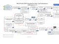
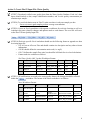
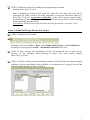
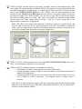
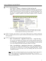
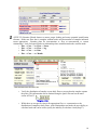
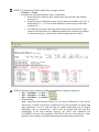
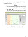
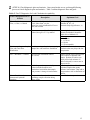
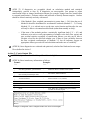
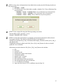
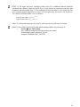
SOP Environmental Quality Assurance (EQA) Standard Operating Procedure Standard Operating Procedure: Estimation of Annual River Pollutant Loads with Flux32 Version 1.2 (Updated 12/01/2010; 12/09/2011; 1/20/2012) Author(s) Karen Jensen, Adam Freihoefer Procedure Description Materials References Contents To calculate the annual pollutant loads for Twin Cities Metropolitan Area rivers using Flux32 software and water quality and flow data collected by the Metropolitan Council Environmental Services (MCES) EQA – Environmental Monitoring and Assessment Unit or other project partners (USGS). • Flux32 software (most recent version). Download at ftp://ftp.usace.army.mil/pub/erdc/EL/Simple_Tools/FLUX_Updates/ • Daily average flows (continuous record of measured and estimated daily flows) • Grab sample water quality concentrations • Manual_IR-W-96_2.pdf: “Simplified Procedures for Eutrophication Assessment and Prediction: User Manual”. William W. Walker. Instruction Report W-96-2. September 1996. Updated April 1999. U.S. Army Corps of Engineers (USACE) • SOP_Flux32_Stream_Load_Estimates_V1.doc • MCES Steps for Flux Analysis_draft_200307.doc • MPCA_FLUX32_Process_Checklist.doc • Summary • Tables • Systematic Operations • Attachments A, B Summary: This SOP outlines the MCES methodology for estimating annual pollutant loads of three major rivers (Mississippi, Minnesota, and St. Croix) from monitored daily average flow and grab sample chemistries using the U.S. Army Corps of Engineers’ software Flux32. Due to differences in input data processing and load estimation methodology, a separate SOP exists for estimating annual loads for monitoring stations located on the tributary streams within the Twin Cities Metropolitan Area. Since flow in the four major rivers responds relatively slowly to precipitation events, MCES and MPCA (Minnesota Pollution Control Agency) staff have determined, based on the MCES sampling frequency, that using a one-year record of average daily flow and grab sample water chemistry data is adequate to estimate annual loads for the major rivers with acceptable uncertainty. The application of a one-year dataset to define an annual river load, rather than multiple years, is acceptable since river events are typically defined as a multi-day record (3 days or greater). The subtle nature of the river system hydrograph, along with consistent frequency of monitoring, allows for a strong statistical relationship when using regressions within Flux. In comparison, the streams possess relatively flashy event hydrographs, at times defining 2 days or less, requiring the stream load estimates to rely on a 3-year dataset. MCES River Load Estimation SOP Page 1 of 16 Annual load estimates for the rivers will be used within the Metropolitan Council benchmark report, annual water quality summary reports, special studies, and shared with external stakeholders. Basic steps for estimation of annual loads include (Figure 1): • Creation of two Flux32 input files per site: average daily flow and water quality (Table 1) • The estimation of loads using Flux32 software. This effort typically requires adjusting flow or seasonal stratification breaks to reduce the coefficient of variance (C.V.) to 0.3 in an effort to reduce the slope in residual plots and ensure that the methods produce similar results • Creation of output text files in specified format to document Flux32 results • Transfer the results to master database of river load results Table 1: Historic MCES and USGS Metropolitan Area River Sites River Name and Mile of Monitoring Station Minnesota River at Jordan Mississippi River at Anoka St. Croix River at St. Croix Falls St. Croix River at Stillwater Mississippi River at Prescott Mississippi River at Lock & Dam 3 Discharge Owner USGS 05330000 USGS 05288500 USGS 05340500 --USGS 05344500 USACE MCES River Load Estimation SOP Discharge Monitoring Record 1934 - Present 1931 - Present 1902 - Present --1928 - Present 1959 - Present Water Quality Owner MCES MN39.4 MCES UM871.6 --MCES SC23.3 --MCES UM796.9 Water Quality Monitoring Record 1979 - Present 1976 - Present --1976 - Present --1976 - Present Page 2 of 16 Figure 1: MCES Flux32 SOP Overview MCES River Load Estimation SOP Page 3 of 16 Action 1: Create Flux32 Input File: Daily Average Flow (STEP 1) Download the average daily flow from the USGS or USACE Website o Minnesota River at Jordan (USGS 05330000) http://waterdata.usgs.gov/nwis/inventory/?site_no=05330000& o Mississippi River at Anoka (USGS 05288500) http://waterdata.usgs.gov/nwis/inventory/?site_no=05288500& o St. Croix River at St. Croix Falls (USGS 05340500) http://waterdata.usgs.gov/nwis/inventory/?site_no=05288500& o Apple River at Somerset, WI (USGS 05341500) (Site used for discharge adjustment) http://waterdata.usgs.gov/nwis/inventory/?site_no=05341500& o Mississippi River at Prescott, WI (USGS 05344500) http://waterdata.usgs.gov/nwis/inventory/?site_no=05344500& o Mississippi River at Lock & Dam #3 (Site used for discharge adjustment) http://www.mvp-wc.usace.army.mil/projects/Lock3.shtml (STEP 2) Ensure that the flow dataset is complete for the period of interest, with no missing data. As outlined in STEP 3, there are two sites that typically have long periods of missing record and therefore need additional modification. (STEP 3) Modification of Average Daily Discharge Flow Record for Three Sites o Mississippi River at Prescott – Average daily discharge from the USGS Mississippi River at Prescott, WI station is measured on a water year basis (Oct-Sept). As a result, when calculating annual loads, there is three months of missing flow data for the previous year. Rather than use a regression to estimate the flow, it was determined that the USACE average daily discharge at Lock and Dam#3 was appropriate to fill in the missing data. Please refer to Attachment A for complete documentation. o St. Croix River at Stillwater – There is no continuous average daily flow monitoring at the location (St. Croix River at Stillwater, MN) where MCES water quality samples are collected. As a result, the discharge is estimated through the summation of the upstream St. Croix River at St. Croix Falls and an upstream tributary Apple River at Somerset. Please refer to Attachment B for complete documentation. o Mississippi River at Anoka – There is no continuous average daily flow monitoring at the location (Mississippi River at Anoka, MN) where MCES water quality samples are collected. As a result, the discharge is estimated by subtracting the Rum River and Elm Creek average daily discharge from the USGS monitoring site approximately 7 miles downstream of Anoka and the MCES site. Please refer to Attachment c for complete documentation. (STEP 4) If not already developed, create an Excel spreadsheet with separate worksheets for each site location as well as a worksheet for notes related to changes and updates made to each dataset. The excel file will serve as the Flux32 Discharge Input File. 4 (STEP 5) Each Excel worksheet should use the following format or append new data to existing input file and update notes page. The notes worksheet should be updated as new data is added each year. o Cell A1 has no effect on Flux and should contain site description and any other relevant information. o Cell B1 should define the flow units used (i.e. ft3/sec) o Site Discharge (MN_JORDAN) Worksheet Format: A B C 1 Site description ft3/sec 2 3 4 DATE 01/01/80 01/02/80 FLOW 10 15 o Notes Worksheet Format. A B D QUALIFIER e C 1 Site description 2 3 4 DATE NOTE AUTHOR 05/26/09 Added 2008 data KMJ 05/28/10 Added 2009 data ATF D (STEP 6) Name flow input file according to following naming convention: Example: River_Discharge_75_09.xls Note: If updating an existing Flux32 input file, update the Notes page and resave file in appropriate file folder with new file name appropriate for the most recent data added (i.e. River_Discharge_75_10.xls). Do not alter existing files, as they will be used to recreate loads if questions arise in future. MCES internal file structure for the storage of Flux32 files is outlined in the Annual WQ Assessment SOP File Location: \NATRES\Assessments \Documents\SOP\SOP_WaterQuality_Assessment_V1.doc 5 Action 2: Create Flux32 Input File: Water Quality (STEP 7) Download verified water quality data from the Water Quality Database. Each site’s data report should include a date, sample identification number, and a water quality concentration per constituent per sample. (STEP 8) To avoid calculation error in Flux32, make sure there is only one sample per date o For two (or more) grab samples per date: average concentration (STEP 9) Create an Excel spreadsheet with separate worksheets for each site location as well as a worksheet for notes related to changes and updates made to each dataset. The excel file will serve as the Flux32 Water Quality Input File. (STEP 10) Each site specific Excel worksheet should use the following format or append new data to existing input file. o Cell A1 has no effect on Flux and should contain site description and any other relevant information. o Cell B1 should define the concentration units used (i.e. mg/L) o Cell C1 defines the sample flow units, but should be left blank for river load calculations o Format each site worksheet as follows: Site Water Quality (MN_Jordan) Worksheet Format: A B C D E F 1 2 3 Site description mg/L STATION DATE Field_Data_ID TP TSS NO3 MI39.4 01/01/80 345678 0.105 549 4.5 4 MI39.4 01/14/80 356780 0.255 1549 1.2 (STEP 11) If modifications are made to the water quality dataset, the changes should be reflected within the worksheet. The format of the Notes worksheet is as follows: Notes Worksheet Format: A B C D E 1 Site description 2 DATE NOTE DATE DOWNLOAD DATA FILE NAME AUTHOR 3 05/26/09 Added 2008 data 05/13/09 River_WQ_76_08.xls KMJ 4 05/28/10 Added 2009 data 05/20/10 River_WQ_76_09.xls ATF 6 (STEP 12) Name flow input file according to following naming convention: Example: River_WQ_76_09.xls Note: If updating an existing Flux32 input file, update the Notes page and resave file in appropriate file folder with new file name appropriate for the most recent data added (i.e. River_WQ_75_10.xls). Do not alter existing files, as they will be used to recreate loads if questions arise in future. MCES internal file structure for the storage of Flux32 files is outlined in the Annual WQ Assessment SOP. File Location: \NATRES\Assessments \Documents\SOP\SOP_WaterQuality_Assessment_V1.doc Action 3: Load Flux32 Input Files for New Project (STEP 13) Open Flux32 executable If starting a New Project: Data → Read → New Sample and Flow Data → New Stratification If opening an existing project: Session → Resumed Saved Session (.FSS File) (STEP 14) After selecting New Stratification, Flux32 will prompt the user to locate the file directory of the discharge (River_Discharge_75_09.xls) and water quality samples (River_WQ_76_09.xls). (STEP 15) Flux32 will first read in the discharge worksheet. If the daily flow file contains multiple worksheets, the user must indicate what worksheet (i.e. monitoring site) is going to be used and column identifier that the flow data is located in. 7 (STEP 16) Flux32 will then read the water quality worksheet. Similar to the discharge input, if the water quality file contains multiple worksheets, Flux32 will prompt user to select the worksheet that contains the appropriate site information (i.e. monitoring site) to be used. Flux32 will next prompt user to select SAMPLE FLOW Field from a list of fields. For river load estimation, the user should select the LOOKUP (Use Daily Flow) since the MCES water quality samples do not have an associated sample flow. MCES typically uses the daily average flow to represent the sample flow when calculating major river loads. Most major river samples are collected as grab samples and the major river flows change relatively slowly – thus use of daily average flow as an approximation of sample flow is appropriate. Note: This differs from stream load estimation as tributary streams are typically flashy and therefore daily average flow is not a good surrogate for event flow. The tributary streams have either a grab or composite flow associated with sample chemistry, and daily average flows are used only to estimate loads for those days without a sample flow. (STEP 17) Flux32 will next prompt user to select the FLUX CONSTITUENT Field from a list of fields. Select field name of parameter to be estimated. (STEP 18) Flux32 will then prompt user to complete the following: o Enter/Modify Site Name: Enter appropriate site name and location. o Confirm input data. Examine the page to make sure number of daily flows and number of samples seems appropriate o Confirm appropriate values for unit conversion. Ensure the conversion factors are correct: 0.894 if using cfs; 1,000 if using mg/l. Use dropdown menus to change values, if necessary. Note: If Flux32 detects duplicate samples, open the water quality input file and manually delete duplicates as described previously in this SOP. Reload data into Flux32. Do not use the Flux32 prompts to delete duplicate samples. 8 Action 4: Estimate Loads with Flux32 (STEP 19) Define Initial Settings o Select Method #6: Method → 6 Regression (3): Daily log c/log q, adj Note: Method 6 is the preferred calculation method as it designed for use with the time series function, which will be used later in this SOP to save data output for yearly, monthly, and daily time steps. (If a load is unable to be calculated using Method 6, the user may use an alternate method and refrain from citing sub-annual time series information. A complete explanation of the Method 6 departure criteria is outlined in Step 27.) o Select Units: Utilities → Preferences → Change • Confirm discharge units are in cfs and concentration units are in mg/L. The Flux Units and Mass Units can be set to whatever the user would like the output to be in (lbs, kg, or metric tonnes) (STEP 20) Examine entire dataset to ensure proper loading and assess potential stratification schemes. Confirm that flow data are complete without breaks and that number of samples indicated seems appropriate. (STEP 21) Set Data filter/screen to include only data period of interest. o Data → Screen/filter data → Apply Date & Value screens → Sample Date Range: For river sites, one calendar year of data are used to develop regression equations used in estimating loads. The max date should be set to the last day of the year of interest (12/31/2009 when estimating 2009 loads). The min date should be set to the first day of year (for estimating 2009 loads, the min date would be 01/01/2009). o Data → Screen/filter data → Apply Date & Value screens → Flow Date Range: For river sites, one calendar year of data are used. The max date should be set to the last day of the year of interest (eg. 12/31/2009 when estimating 2009 loads). The min date should be set to the first day of year (for estimating 2009 loads, the min date would be 01/01/2009). Note: Once dates are changed using data screen, do not simply change the dates again to re-filter data, as an error occurs and data will not be loaded properly. To reset dates: Data → Screen/filter data → Apply Date & Value screens → Reset and then repeat date filter process described above. 9 (STEP 22) Examine filtered dataset to ensure proper loading and assess potential stratification schemes. Make sure flow data is complete without breaks and that number of samples indicated seems appropriate. Examine plots for concentration vs. flow or concentration vs. season relationships. Look for logical breaks in relationship where stratification breaks could be made. o Plot → Conc → vs. Flow → linear o Plot → Conc → vs. Flow → log o Plot → Conc → vs. Date o Plot → Conc → vs. Month o Verify the distribution of samples versus daily flows to ensure that the samples capture the peaks. This information can be obtained using the Quick Plot tool on the main screen of Flux32. o While there are no specific criteria for appropriate flow vs. concentration or the distribution of samples to daily flows, weak relationships can hinder the users ability to calculate loads and can be used to justify the inability to calculate a load (Step 27). 10 (STEP 23) Calculate initial loads (which relies on single stratum) o Calculate → Loads o Examine Flow and Load Summary output. In particular: Do the daily flow statistics agree with the dates selected in the data filtering process (#1)? Is the Flux (kg/y) similar between the various statistical methods (1-6) (#2)? Is the Method 6 C.V. < 0.2? How do the Method 6 results compare to the other methods (#3)? The inability to meet the following criteria does not necessarily mean a load cannot be calculated; however, additional modifications to the data as outlined in subsequent steps (i.e. stratification, method change) may be needed. (1) (2) (3) (STEP 24) Examine initial qualitative (graph) and quantitative (statistics) diagnostics. o Plot → Residuals → vs. Flow → o Plot → Residuals → vs. Date → o Plot → Residuals → vs. Month → o When plotting Note: Input data and associated loads for a river may be influenced by flow and by date/season, in which case the flow residual plot may look acceptable (no slope, high slope significance, low R2) while the date or month residual plots may be sloped, indicating a date or seasonal bias. Flux32 does not include both date and flow relationships in the load estimates; however, the USGS load estimation tool (LOADEST) does have that capability. With Flux32, the user must choose to either minimize flow residuals or minimize date/seasonal residuals using stratification. 11 (STEP 25) Upon examining the initial load results using a single stratum, the user has the option of assigning multiple strata based on discharge or seasonal / date. The objective is to reduce the C.V. and minimize residual slopes. o Stratify data: Data → Stratify → On Flow On Hydrograph On Season On Date o On Flow Stratification: Typically relies on two strata (split at Qmean) or three strata (split at ½ Qmean and split at 2x Qmean). Upon choosing one of the flow strata, the user can then manually edit the strata boundaries through numeric or graphical means. If the user would prefer to manually enter all of the strata breaks, use Data → Stratify → On Flow → Other o On Season Stratification: Stratification breaks often correlate with winter (midOctober – January), spring (February – mid May), summer (mid-May – mid-August), and fall (mid-August – mid-October). Examining the graphical interface will assist the user in appropriately identifying strata breaks. o On Date Stratification: Using the date function allows the user to break up strata while viewing the hydrograph. Similar to the season stratification, it is recommended that the user identify and define strata breaks with the graphical interface. 12 (STEP 26) Check diagnostic plots and statistics: Once strata breaks are set, go through following process to check diagnostic plots and statistics. Table 2 outlines diagnostic tests and goals. Table 2: Flux32 Diagnostics for Load Calculation Acceptability Flux32 Diagnostic Plot or Statistic Description Optimum Goal Plot → Residuals → vs. Flow, vs. Date, vs. Month Examine residual plots for bias; Click “Show Stats” on plot. Often bias can be eliminated for Flow or Date, but not both No slope (slope ≈ 0) Minimize R2 (R2 ≈ 0) Maximize Slope Significance ( ≈1) Calculate → Loads Creates summary table of load by method; also gives C.V. by method Flow weighted concentration estimate for Method 6 should be within 20% of Methods 3-5. C.V. range 0 - 0.1 (Good) 0.1 - 0.2 (Fair) > 0.2 (Poor) > 0.3 (Unacceptable) Provides information about distribution that may help with data interpretation Calculate → Compare Sample Provides a variety of statistics comparing Flow with Total Flow sample flow with total flow distribution Distribution List → Residuals → Outliers Provides lists of statistical outliers (P<=0.050) List → Jackknife Table Jackknife procedure systematically deletes individual samples and recalculates load without that sample, then presents % change in load estimate. List → Breakdown by Stratum and Optimum Sampling Can provide information about optimizing sample collection during future efforts. Outliers should only be deleted with some evidence of problem with sample. Deletion of outliers can greatly affect load estimates. If outlier is deleted, be sure to note in output text file. Look through table and identify individual samples that greatly influence load estimate. May add in interpretation or aid in elimination of outliers. Can aid in data interpretation. 13 (STEP 27) If diagnostics are acceptable (based on calculation method and statistical relationships), proceed to Step 28. If diagnostics are unacceptable, first attempt to adjust stratification breaks or change stratification scheme (for example, change from flow stratification to seasonal stratification). Evaluate outliers and jackknife to identify aberrant samples. Outliers should be deleted cautiously and only with reason. o If the Method 6 flow weighted concentration is greater than +/- 20%, then the use of Method 6 should be abandoned for an alternative methods (Methods 3 – 5). If using Methods 3-5, it is advised not to use the time series function and therefore the user will only be able to cite annual modeled loads (rather than monthly or daily). o If the none of the methods produce a statistically significant load (C.V. < 0.3) and indicators exist such as weak representation of samples to the daily flow regime and poor residual statistics regardless of stratification scheme, you may not be able to calculate a load for the specified calendar year. If there is some variability between the flow weighted concentrations of Methods 3-5, but all indicators suggest an appropriate dataset, proceed will load calculation and make note of variability. (STEP 28) Once diagnostics are evaluated and optimized, calculate final loads and create output file as defined in Action 5. Action 5: Create Output File (STEP 29) Open text editor like “Notepad” or “Notetab Light” (STEP 30) Enter introductory information as follows: Format: Example: Line Line 1 2 3 4 5 6 7 Site name, parameter, year of interest 1 Minnesota River at Jordan. Nitrate (2009) 2 04/15/2010; Adam Freihoefer Version of Flux32 3 Flux32 Version 1.1.2 (3/10/09) Input files Stratification breaks Outliers deleted 4 5 6 Notes: 7 River_Discharge_75_09.xls; River_WQ_75_09.xls Seasonal (4 Strata) (01/01, 04/07, 07/26, 10/01) No Outliers Deleted Note: While flow residuals look good, monthly residuals are biased (sloped) Date of analysis and analyst name Example of Required Flux32 Output Header Per Each Load Output 14 (STEP 31) Once above information has been added, then cut and paste the following into the text file, in this order: o Calculate → Loads o To calculate time series loads (daily, monthly, calendar) Use 1 Day as Maximum Gap for Interpolation - Calculate → Series → Calendar Year (1 Day as Maximum Gap for Interpolation) - Calculate → Series → Monthly (1 Day as Maximum Gap for Interpolation) - Calculate → Series → Daily (1 Day as Maximum Gap for Interpolation) (STEP 32) Save output file using the following naming convention: Sitenameabbreviation_parameter_year.txt Example: MNJORD_NO3_2009.txt (STEP 33) Load values and statistics are manually extracted and summarized within a historic river loads worksheet. The location of the MCES River Loads dataset is: NATRES\Assessments\WQ_Load_Calculations\2009\Output_Files\Rivers\2009_River_WQ_L oad_Dataset.xlsx If additional load data is added to the 2009_River_WQ_Load_Dataset.xlsx the user should update the Notes worksheet. Information provided within the 2009_River_WQ_Load_Dataset.xlsx includes: o Site o Parameter o Analysis period o Stratification scheme and divisions o Calculation method o Samples used / excluded o Observed flow volume o Flux modeled mass and concentration o Flux interpolated mass and concentration o CV (Coefficient of Variation) o Upper and lower limits of 95% confidence interval (Step 34) 15 (STEP 34) The upper and lower confidence limits of the 95% confidence interval should be calculated and reported within the MCES River Loads dataset in conjunction with the other parameters indicated within Step 33. The method to calculate the limits is cited within the Flux user’s manual entitled Simplified Procedures for Eutrophication Assessment and Prediction: User Manual (William Walker, 1999) as follows: Lower Limit value = Ym * e(-2 * CV) Upper Limit value = Ym * e(2 * CV) where Ym is the predicted mean value and CV is the error mean coefficient of variation. (STEP 35) Save Flux32 Session File using similar naming scheme as used in Step 32. o Session Æ Save This Session Save output file using the following naming convention: Sitenameabbreviation_parameter_year.txt Example: MNJORD_NO3_2009.FSS 16