Download Ball, I.R., and H.P. Possingham, 2000. MARXAN (V1.8.2)

Marxan (v1.8.2)
Marine Reserve Design using Spatially Explicit Annealing
A Manual Prepared for The Great Barrier Reef Marine Park Authority
Ian Ball
Hugh Possingham
March 2000
Acknowledgements
Marxan is the marine version of Spexan. Spexan was funded by Environmental
Australia and was based on the FORTRAN77 program SIMAN. SIMAN was
written at the University of Adelaide at their excellent department of applied
mathematics. At Environment Australia, Spexan was supported by Andrew
Taplin who contributed ideas about the problems which it should solve.
The new interface was originally suggested by Eli Meir with significant
contributions from Drew Tyre. Marxan was developed under contract to the
Great Barrier Reef Marine Park Authority who’s Representative Areas Program,
Analytical Working Group contributed the main ideas which differentiate this
program from Spexan. In particular Hugh Possingham and Trevor Ward helped
nail the main concepts into working rules. Trevor Ward contributed many useful
comments about this manual and Suzanne Sleger had most of the bugs in the
beta version happen to her.
Additional support has been funded by the National Marine Fisheries Services
through the very helpful collaboration of Mary Ruckelshaus.
1
Table of Contents
Acknowledgements _____________________________________________ 1
Table of Contents _______________________________________________ 2
New to Marxan v1.8 .................................................................................................5
Outline of this Manual .............................................................................................6
1 CONCEPTS __________________________________________________ 7
1.1 Basic Concepts of Reserve Selection ..............................................................7
1.2 The Objective Function .....................................................................................8
1.2.1 Cost of the Reserve System .......................................................................9
1.2.2 Boundary Length and Fragmentation ........................................................10
1.2.3 Representation Requirements for Conservation Features.........................10
1.2.4 Conservation Feature Penalty...................................................................11
1.2.5 Spatial effects on the conservation feature penalty ...................................13
1.2.6 Conservation Feature Penalty Factor........................................................15
1.2.7 Cost Threshold Penalty.............................................................................15
1.3 Optimisation Methods for the Objective Function ........................................16
1.4 Iterative Improvement......................................................................................16
1.5 Simulated Annealing .......................................................................................16
1.5.1 Selecting the Initial Reserve System .........................................................18
1.5.2 Number of Iterations .................................................................................18
1.5.3 Temperature .............................................................................................18
1.5.4 Adaptive Annealing Schedule ...................................................................19
1.5.5 Fixed Schedule Annealing.........................................................................19
1.5.6 General Process for setting a fixed schedule ............................................20
1.6 Heuristics .........................................................................................................20
1.6.1 Greedy Heuristics .....................................................................................21
1.6.2 Richness ...................................................................................................21
1.6.3 Pure Greedy..............................................................................................22
1.6.4 Rarity Algorithms.......................................................................................22
1.6.5 Maximum Rarity ........................................................................................22
1.6.6 Best Rarity ................................................................................................23
2
1.6.7 Summed Rarity .........................................................................................23
1.6.8 Average Rarity ..........................................................................................23
1.6.9 Irreplaceability...........................................................................................24
1.6.10 Product Irreplaceability............................................................................24
1.6.11 Summed Irreplaceability..........................................................................24
2 USING THE PROGRAM ________________________________________ 26
2.1 Setting the Scenario ........................................................................................26
2.1.1 Basic changes to the input files.................................................................26
2.1.2 Boundary Length Modifier .........................................................................27
2.1.3 Cost Threshold..........................................................................................27
2.2 The Solution Method .......................................................................................28
2.2.1 Simulated Annealing .................................................................................28
3 SETTING UP THE INPUT FILES__________________________________ 31
3.1 Command Line Parameter ..............................................................................31
3.2 Planning Unit File ............................................................................................32
3.3 Conservation Feature File...............................................................................33
3.4 Block Definition ...............................................................................................34
3.5 Boundary Length File ......................................................................................36
3.6 Planning Unit versus Conservation Feature File...........................................37
3.7 Input Parameter File ........................................................................................38
4 MARXAN OUTPUTS ___________________________________________ 44
4.1 Screen Output ..................................................................................................44
4.2 File Output........................................................................................................45
4.2.1 Solutions for each run ...............................................................................46
4.2.2 Missing Values for each run ......................................................................46
4.2.3 Best Solution for all runs ...........................................................................46
4.2.4 Summary Information................................................................................48
4.2.5 Scenario Details........................................................................................49
4.2.6 Summed Solution......................................................................................49
REFERENCES _________________________________________________ 51
Appendix A: Differences Between Marxan and Spexan _______________ 52
3
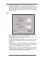
Appendix B: Using Inedit.Exe ____________________________________ 54
Problem .............................................................................................................54
Run Options.......................................................................................................55
Annealing...........................................................................................................56
Input...................................................................................................................57
Output................................................................................................................58
Cost Threshold ..................................................................................................60
Misc ...................................................................................................................61
Appendix C: Old Style File Formats _______________________________ 62
General ...................................................................................................................62
Input Files ..............................................................................................................62
input.dat .............................................................................................................62
Cost.dat .............................................................................................................63
Species.dat ........................................................................................................64
Bound.dat ..........................................................................................................65
Pustat.dat ..........................................................................................................65
PUvSP.dat .........................................................................................................66
PUvSPr.dat ........................................................................................................66
PUXY.dat ...........................................................................................................66
name.dat............................................................................................................67
Index_________________________________________________________ 68
4
New to Marxan version 1.8
Appendix A contains a detailed list of changes and feature additions. The main
features recently added include:
•
New Iterative Improvement variations.
•
New snapshot saving to allow viewing an evolving solution.
•
New PuvCF file allowable. Marxan can detect which type is used.
•
New log file output
•
More complex clumping options.
New to Marxan v1.0
Appendix A contains a detailed list of differences between Marxan and Spexan.
Marxan contains a number of quite new features which include:
!
Self annotated and robust input file formats
!
Improved spatial possibilities. In Marxan there is no limit on the target
number of planning units which you can have mutually separated by a
safe distance
!
Block definition of targets. In Marxan you can set a type for a
conservation feature and then set default targets for all conservation
features of that type.
!
New target types.
!
A block definition can be of the form x% of total amount available.
!
In addition to having an amount target you can have a target number
of occurrences.
!
Summed Solutions: a new way to explore irreplaceability.
!
Output files can now be of the csv type which Arcview can read in
directly.
5
Outline of this Manual
This manual is separated into several conceptually separated sections. Section
One covers the methods used in Marxan. This includes a description of the
objective function and how each element contributes to its value and a detailed
description of how each of the optimisation methods has been implemented.
Section two describes how to solve reserve selection problems. This includes the
main options for testing scenarios and ways to tune the optimisation function. It
is worthwhile for a new user of the program to read this section as it contains
advice on which settings to try out first.
Section three contains a format description for all of the input files. It contains a
useful description of each of the parameters which are entered in the main
parameter option file. It is useful to read this in conjunction with Appendix B
which describes the windows interface program Inedit.exe which is a convenient
way to edit the main control parameters.
Section four describes the format of the output files from Marxan. It also
described how the output files can be used.
There are three appendices. The first one is a change history since version 1.0.
Appendix B is a manual for the Inedit.exe windows interface. For a windows user
it would be worthwhile having Appendix B printed out and at hand when using
the program. Appendix C contains an input file format description for the old file
format. It is possible to force Marxan to use the old file formats but it will not then
be able to use many of the new features. The only reason to use the old file
formats is if they are already created – possible for Spexan or an old version of
Marxan.
6
1
CONCEPTS
This section includes a description of the basic concepts of reserve selection and
the objective function approach which is used in Marxan. The main concepts
which appear in this section are:
1.1
!
Basic concept of reserve selection.
!
The two approaches to reserve selection - heuristics and optimisation
!
The Main Objective function
!
Additions to the objective function
!
Simulated annealing and how it works
!
Heuristics and how they work.
Basic Concepts of Reserve Selection
Marxan was developed to aid in the design of reserve systems. It was designed
for marine reserve systems based on the terrestrial reserve design software
Spexan. Both are basic extensions of a FORTRAN77 program SIMAN which
contained the main concepts but not in a fashion which was easy for non-experts
to use.
The basic idea is that the reserve designer has a large number of potential sites
or planning units from which to select a reserve system. They wish to devise a
reserve system which is made up of a selection of these planning units which will
satisfy a number of ecological, social and economic criteria.
Typically these criteria could be: That certain specific species or conservation
features are well protected within the reserve system; That all defined habitat
types are sufficiently protected by the reserve system; Perhaps that certain
planning units with particular cultural heritage (In a marine setting this could be a
planning unit containing a noteworthy ship-wreck) are included in the reserve
system; That the reserve system does not unnecessarily impact upon industries
within the region.
There is a great deal of subtlety in setting these requirements and a large
amount of detail which the reserve designer might wish to include. Marxan can
aid in the design of a reserve system using a great deal of the detail that is
available. It is designed to produce reserve systems which the designer might
then alter to take into account information which could not easily be quantified. It
is also designed to help automate the design process so that a designer can try
many different scenarios and see what the resulting reserve systems might look
like. It could also be used to try to produce reserve systems which are all quite
different to help a designer break out of some pre-conceived pattern of planning
unit selection.
A way of dealing with these requirements is to have well defined targets for all of
the conservation features and well defined measures of the economic impact of
the reserve system. The targets then become design constraints and the impact
7
is the cost of the design, with a minimal cost being desirable. Social costs are
then split up into things which an economic cost can be put on, things which can
be handled by treating them as a conservation feature, and things which have to
dealt with specially. The things which do not fall into the simple cost/constraint
categories are not dealt with by the Marxan software but by the designer. This is
done by forcing planning units into the system before the software is applied or
by altering the reserve system afterward.
Once the basic requirements and costs are understood there are two main
methods for designing the reserve system using Marxan. Historically the first is
the ‘heuristic method’ where a rule of thumb is used to add reserves to a system
until all of the reserve requirements are met. The other is using an objective
function whereby any collection of planning units can be given a score
depending upon how good that collection is as a reserve system. Then an
optimisation method can be applied to attempt to find the collection of planning
units which has the best score according to the objective function. Both of these
approaches are described below. In Marxan the main optimisation method is
simulated annealing, although the objective function principal works with other
optimisations methods including one of the heuristic methods (the greedy
algorithm).
1.2
The Objective Function
The objective function gives a value for a collection of planning units as if that
collection constituted a reserve. This means that even a single planning unit or
no planning units at all can be given an objective function value. A reserve
containing zero planning units would be cheap to implement, but it would
probably not meet all (or indeed any) of the ecological requirements and so the
objective function value should be very poor.
If we have an objective function which gives any possible reserve system a
value, or score, then we can compare any two reserve systems and say which
one is better than the other (according to the objective function at least).
Because the objective function value can be evaluated by a computer the door is
open to using a wide range of methods to automatically create reserve systems
which have good objective function values.
The objective function which is used in Marxan is designed so that the lower the
value the better the reserve. In its simplest form it is a combination of the
economic cost of the reserve and a penalty for not meeting all of the ecological
objectives, if any are unmet.
In Marxan this objective function is used by the greedy heuristic the iterative
algorithm and by simulated annealing. The objective function was designed with
the aim to integrate it with a simulated annealing optimiser but the two are
distinct entities. Simulated annealing is a general purpose optimiser and the
objective function defines what is desirable in a reserve system without explicitly
defining how an optimal reserve will be found.
The objective function consists of two main sections; the first is a measure of the
‘cost’ of the reserve system and the second a penalty for breaching various
criteria. These criteria can include a cap on the ‘cost’ of the reserve system and
always includes the target representation level for each conservation feature. As
8
well as this is the optional measure of the fragmentation of the reserve and an
optional cost threshold penalty. In this objective function the lower the value the
better the reserve system.
∑ Cost + BLM ∑ Boundary + ∑ CFPF × Penalty + Cost Threshold Penalty( t )
Sites
Sites
ConValue
Here the cost is some measure of the cost, area, or opportunity cost of the
reserve system. It is the sum of the cost measure of each of the sites within the
reserve system.
‘Boundary’ is the length (or possibly cost) of the boundary surrounding the
reserve system. The constant BLM is the boundary length multiplier which
determines the importance given to the boundary length relative to the cost of
the reserve system. If a value of 0 is given to BLM then the boundary length is
not included in the objective function.
The next term is a penalty given for not adequately representing a conservation
feature, summed over all conservation features. CFPF stands for ‘conservation
feature penalty factor’ and is a weighting factor for the conservation feature
which determines the relative importance for adequately reserving that particular
conservation feature. The penalty term is a penalty associated with each underrepresented conservation feature. It is expressed in terms of cost and boundary
length and is roughly the cost and additional modified boundary needed to
adequately reserve a conservation feature which is not adequately represented
in the current reserve system.
The cost threshold penalty is a penalty applied to the objective function if the
target cost is exceeded. It is a function of the cost and possibly the boundary of
the system and in some algorithms will change as the algorithm progresses
(which is the t in the above formula). This penalty is also optional and can be
excluded from the objective function.
1.2.1 Cost of the Reserve System
The cost of the reserve system can be any of a number of measures. The
objective function that Marxan uses has the constraint that the cost of a reserve
system is the linear combination of costs of all the planning units within the
reserve system.
This works well under a variety of cost structures. If the cost were simply the
number of planning units or the total area taken for the reserve system then
obviously the cost of each individual planning unit (either 1 or its area) can be
added together to get an accurate cost measure for the reserve system as a
whole.
For complex economic costs this can only be an estimate of the true economic
cost. Here the way to include them is to work out an initial estimate of the
economic cost for each planning unit for each economic factor of interest and to
combine these into a single economic cost for the planning unit. Once a reserve
system has been designed using this cost structure the actual (modelled)
9
economic cost for the system could then be generated and areas where the
initial estimate is inaccurate can be identified for further work.
1.2.2 Boundary Length and Fragmentation
It is desirable for the reserve system to be not too fragmented. One simple way
to measure (and hence control) fragmentation is to take the length of the
boundary between planning units within and outside of the reserve system. For a
reserve system of any fixed size the lower the boundary length the more
compact and less fragmented the reserve system. By including a boundary
length term in the objective function we can apply a control on the level of
fragmentation in the designed reserve system.
In order to allow the boundary length to be added to the cost measure a
multiplicative factor is used. This is because the boundary length is most
probably going to be in units which are different from the cost measure. It is
theoretically possible to put a dollar cost on each boundary and if a dollar cost is
also put on each planning unit then the boundary length modifier is not
important, but this is an exceptional case. In general not only are the units
incompatible without a boundary length modifier, but the importance of
compactness over reserve cost are not immediately obvious. Changing the
boundary length modifier allows the reserve designer to explore this issue.
1.2.3 Representation Requirements for Conservation Features
The representation requirements for the conservation features can be
moderately complex. In the objective function if the conservation feature does
not meet one or more of it’s requirements then it will attract a penalty depending
upon how far below representation it is and the relative value of the conservation
feature to the other conservation features. This penalty is discussed in the next
section.
The simplest representation requirement is that a single occurrence of the
conservation feature is adequate. This can be generalised to any number of
occurrences as a target and can be substituted for, or combined with, a target
amount. The target amount could be an area, which would make sense for a
vegetation or habitat type, or a population amount, if population estimates were
being used.
In addition to this there are a couple of spatial requirements which could be
included, an aggregation and a separation requirement. The first guards against
unviable populations or target areas and the second is a risk spreading
mechanism.
In addition to the target area requirement another requirement can be included
that none of the patches of that conservation feature are too small. The idea
being that an area target of 100 hectares wouldn’t be made up of 400 separate
quarter hectare blocks when it is known that the given conservation feature is not
viable on such a fragmented landscape. Thus a second target can be set which
is the minimum viable patch for that conservation feature. This patch could be
made up of a number of smaller adjacent planning units or from parts of a
number of adjacent planning units.
10
The separation requirement, if set for a conservation feature, is that a given
number of planning units holding that conservation feature within the reserve
system must be mutually separated. Thus the target might be that at least 4
planning units are mutually separated by a distance of 100 kilometres. This type
of requirement helps protect against the dangers of a localised disaster
destroying the total reserve holding of the given conservation feature. It can have
the possible added effect of increasing the diversity of the holding for the
conservation feature, by picking representation of that conservation feature over
a greater geographic range.
The separation requirement can be used in conjunction with the aggregation
requirement. Here the planning units which must be mutually separated must
come from viable patches.
Note that the separation requirement deals with planning units instead of
patches. This means that if a conservation feature is widespread enough and the
reserve system is large enough, then the separation requirement could be
theoretically met by one very large patch of the conservation feature. The aim of
the requirement is to spread the holdings of the conservation feature
geographically, not to encourage fragmentation of that conservation feature’s
holding.
1.2.4 Conservation Feature Penalty
The conservation feature penalty is the penalty given to a reserve system for not
adequately representing conservation features. It is based on a principle that if a
conservation feature is below its target representation level, then the penalty
should be close to the cost for raising that conservation feature up to its target
representation level. For example: if the requirement was to represent each
conservation feature by at least one instance then the penalty for not having a
given conservation feature would be the cost of the least expensive planning unit
which holds an instance of that conservation feature. If you were missing a
number of conservation features then you could produce a reserve system that
was fully representative by adding the least expensive planning units containing
each of the missing conservation features. This would not increase the objective
function value for the reserve system, in fact, if any of the additional planning
units had more than one of the missing conservation features, then the objective
function value would decrease.
It would appear to be ideal to recalculate the penalties after each change had
been made to the reserve system. However, this would be time consuming and it
turns out to be more efficient to work with penalties which change only in the
simplest manner from one point in the algorithm to the next.
A greedy algorithm is used to calculate the cheapest way in which each
conservation feature could be represented on it’s own and this forms the base
penalty for that conservation feature. Marxan adds together the cheapest
planning units which would achieve the representation target. This approach is
described in the following pseudo-code:
I.
For each planning unit calculate a ‘cost per hectare’ value.
11
A.
Determine how much of the target for the given conservation
feature is contributed by this planning unit.
B.
Determine the economic cost of the planning unit
C.
Determine the boundary length of the planning unit
D.
The overall cost is economic cost + boundary length x BLM
(Boundary Length Multiplier)
E.
cost-per-hectare is then the value for conservation feature
divided by the overall cost.
II.
Select the planning unit with the lowest cost-per-hectare.
Add it’s cost to the running cost total and the level of
representation for the conservation feature to the representation
level total.
A.
If the level of representation is close to the target then
it might be cheaper to pick a ‘cheap’ planning unit has the
required amount of the conservation feature regardless of
it’s cost-per-hectare.
III. Continue adding up these totals until you have found a
collection of planning units which adequately represent the given
conservation feature.
IV.
The penalty for the conservation feature is the total cost
(including boundary length times boundary modifier) of these
planning units.
Thus, if one conservation feature were completely unrepresented then the
penalty would be the same as the cost of adding the simple set of planning units,
chosen using the above code, to the system, assuming that they are isolated
from each other for boundary length purposes. This value is quick to calculate
but will tend to be higher than optimum. There might be more efficient ways of
representing a conservation feature than that determined by a greedy algorithm,
consider the following example.
Example 1: Conservation Feature A appears on a number of sites, the best ones
are:
Planning Unit
Cost
Amount of A
represented
1
2.0
3
2
4.0
5
3
5.0
5
4
8.0
6
The target for A is 10 units. If we use the greedy algorithm we would represent
this with planning units 1, 2, and 3 (selected in that order) for a total cost of 11.0
units. Obviously if we chose only planning units 2 and 3 we would still adequately
represent A but our cost would be 9 units.
This example shows a simple case where the greedy algorithm does not produce
the best results. The greedy algorithm is rapid and produces reasonable results.
The program will tend to overestimate and never underestimate the penalties
when using a greedy algorithm. It is undesirable to have a penalty value which is
too low because then the objective function might not improve by fully
representing all conservation features. If there are some conservation features
which need not be fully represented this should be handled entirely by use of the
conservation feature penalty factor, which is described below. It is not
problematic to have penalties which are higher then they absolutely need to be,
12
sometimes it is desirable. The boundary cost for a planning unit in the above
pseudo-code is the sum of all of its boundaries. This assumes that the planning
unit has no common boundaries with the rest of the reserve and hence will again
tend to overestimate the cost of the planning unit and the penalty.
The penalty is calculated and fixed in the initialisation stage of the algorithm. It is
applied in a straight forward manner - if a conservation feature has reached half
of its target then it scores half of its penalty. The problem with this is that you
might find yourself in a situation where you only need a small amount to meet a
conservation feature’s target but that there is no way of doing this which would
decrease the objective value. If we take Example 1 once again, then the penalty
for conservation feature A is 11 units (see above). If you already have planning
units 1 and 4 in the nature reserve then you have 9 units of the conservation
feature and the penalty is 11.0 x (10-9)/10 = 1.1 units. So the species attracts a
penalty of 1.1 units and needs only 1 more unit of abundance to meet its target.
There is no planning unit with a cost that low - the addition of any of the
remaining planning units would cost the reserve system much more than the
gain in penalty reduction.
This problem can be fixed by setting a higher CFPF (Conservation Feature
Penalty Factor) for all conservation features. The CFPF is a multiplicative factor
for each conservation feature, described below.
It is quite possible that the target for a conservation feature is set higher than
can possibly be met. In Australia where the JANIS (1997) requirements state
that 15% of the pre-European area of each forest ecosystem type should be
reserved, we can easily have targets which are larger than the current area of a
given forest ecosystem. Currently, when this is the case, the algorithm will scale
up the penalty so that if, for example, it costs 100 units to reserve all of a given
ecosystem but that represents only half of the target, then the initial penalty will
be 200 units. This means that if you get half-way to your target then the penalty
for that conservation feature will be half the maximum penalty, no matter how
high the target or whether it is a feasible target.
1.2.5 Spatial effects on the conservation feature penalty
When calculating the initial penalty for a conservation feature which has spatial
requirements a different method is used. In this case a very simple estimation is
made for conservation features which are subject to an aggregation and to a
separation rule. Planning units which contain the conservation feature are
collected at random until the collection meets the target and the spatial
requirements for the conservation feature. At this point there are superfluous
planning units in the collection and these are removed. The remaining planning
units are then scored and this is the penalty for that conservation feature. Here
the greedy method has been replaced with an iterative improvement method.
A conservation feature which has a spatial aggregation rule has a second target
value which is the smallest amount of contiguous patches which will count to the
main target. A patch is a group of contiguous planning units, on each of which
the given conservation feature occurs. The second target should be something
13
like the minimum viable population size (or minimum clump size) for a species or
the area required for such a minimum viable population. If a group of contiguous
planning units contain a conservation feature but not as much as the minimum
clump size then the reserve system is penalised for that conservation feature as
if none of those planning units contained the conservation feature.
More advanced penalties for sub-sized clumps are available in version 1.8 of the
software. Instead of the clump not counting at all toward that conservation
features amount it can count half of it’s value. Another alternative is that the
scaling factor for the amount that a clump contributes is proportional to the
proportion of the minimum clump size met. In this case if the clump size is half of
the minimum clump then the amount contributes half of its value to the
conservation factors. In all cases if a clump is larger than the minimum clump
size then there is no penalty and the amount contributes directly to the total
amount for that conservation feature.
The two alternative clumping rules may be useful in encouraging clumping of
selected sites but they are inconsistent with the concept of a minimum clump
size relating directly to a quantity such as a minimum viable population size. This
is because they will both tend to meet some of a conservation feature’s target
with fragments of that conservation feature (possibly contained in clumps of
other conservation features of large size). They could be used where clumping is
to be encouraged but the minimum clump size is not as rigid as a minimum
viable population size.
The separation rule is handled in an even simpler way. Algorithms which use this
option look through all the planning units for the given conservation feature and
determine if there are enough of them at the required separation distance from
each other. This separation distance must be specified for each conservation
feature which follows the separation rule. The program determines whether there
are one, two, or three or more planning units which are mutually separated by at
least this distance. The maximum number of planning units in valid patches
which are mutually separated by the given distance is the separation count of
that conservation feature. If a conservation feature has a separation count that is
lower than the target separation then a penalty is added. This penalty is a
number which is multiplied against the base penalty for the conservation feature
(the penalty when there is not holding for that conservation feature) and then
added to the conservation feature’s penalty.
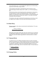
This separation penalty function is:
penalty =
1
7 * C p + 0.2
−
1
7.2
Here C p is the separation count for the conservation feature as a fraction of the
target separation count. If separation count is zero then the separation count is
set to 1 / target separation count. The values 7 and 0.2 were chosen after
experimentation to give a sensible separation penalty multiplier under a wide
variety of conditions.
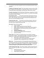
As the separation count increases from 1/target separation count to 1 this
penalty looks like:
14
S e p a r a tio n P e n a lty M u lt ip lie r
Multiplier
1 .5
1 .0
0 .5
0 .0
0 .0
0 .1
0 .2
0 .3
0 .4
0 .5
0 .6
0 .7
0 .8
0 .9
1 .0
P r o p o r tio n o f S e p a r a tio n T a r g e t
Figure 1: Separation Penalty Multiplier as a function of the proportion of the separation
target met. Note that separation targets are normally low integers so only some values of
the multiplier can be taken on.
1.2.6 Conservation Feature Penalty Factor
The conservation feature penalty factor (CFPF) is a multiplicative factor which
can be unique to each conservation feature. It is primarily based on the relative
worth of that conservation feature but it includes a measure of how important it is
to get it fully represented. The actual effect that it will have varies between the
methods which use the objective function. If it is below 1 then the algorithm
might well refuse to add a planning unit to preserve that conservation feature if
there are no other conservation features on the planning unit.
An algorithm might well fall slightly short in the representation of species, getting
close to, but not at or above, the target value. To ensure that each conservation
feature (which can meet its target) meets the target it can sometimes be
desirable to set the CFPF at much greater value than 1.
1.2.7 Cost Threshold Penalty
This has been included to make it possible to look at a reverse version of the
problem. The reversal of the problem would be to find the reserve system which
has the best representation for all conservation features constrained by a
maximum cost for the reserve system. The cost threshold penalty is included to
try to tackle this problem using the framework built to solve the traditional
problem. It works by applying a penalty to the objective function if the cost of the
system has risen above the desired threshold. The threshold is based around the
cost of the system only and doesn’t include boundary length. When running the
15
heuristic algorithms with a cost threshold they will simply stop adding planning
units to the system when the threshold is reached. Simulated Annealing,
however, allows the system to go above the cost threshold but the penalty will
drive it back down in the end. The level of the penalty varies according to the
progress of the simulated annealing algorithm as described below.
1.3
Optimisation Methods for the Objective Function
There are three optimisation methods for the objective function. The iterative
improvement algorithm, the simulated annealing algorithm and the greedy
heuristic. The final of these is described in the heuristics section. The other two
are described here.
1.4
Iterative Improvement
Iterative improvement is a simple optimisation method. It has largely been
supplanted by simulated annealing but can still be profitably used to aid the other
algorithms.
There are three basic types of iterative improvement which can be used in
Marxan. They differ in the set of possible changes which are considered at each
step. Each of them start with a ‘seed’ solution. This can be any kind of reserve
system with some, all, or no planning units contained in the system. It is useful to
use the final result from another algorithm such as simulated annealing as the
starting solution for iterative improvement. In this case the iterative improvement
algorithm is used solely to ensure that no simple improvements are possible.
At each iteration the algorithm will consider a random change to see if it will
improve the value of the objective function if that change were made. If the
change does improve the system then it is made, otherwise another, as yet
untested, change is tested at random. This continues until every possible change
has been considered and none will improve the system. The resulting reserve
system is a local optimum.
The three basic types of iterative improvement differ in the types of change that
they will consider. The simplest type is called ‘normal iterative improvement’ and
the only changes that are considered are adding or removing each planning unit
from the reserve system. This is the same ‘move set’ as is considered by the
greedy algorithm and by simulated annealing.
The second type of iterative improvement is called ‘swap’ and it will randomly
select planning units, if the selected planning unit can improve the system by
being added or removed from it then this is done otherwise an exchange is
considered. If the chosen planning unit is already in a reserve system then the
changes considered are removing that planning unit but adding another one
somewhere else. If the chosen planning unit is not in the reserve system then
the changes considered are adding this to the reserve system but removing one
that is already in the system. Every possible ‘swap’ is considered in random
order, stopping when one is found which will improve the system. Because the
number of possible exchanges can be very large, this is a much slower option.
16
The third type is called ‘two step’, in this method as well as testing each planning
unit (in random order) to see if adding or removing it would improve the system,
each possible combination of two changes is considered. These changes
include, adding or removing the chosen planning unit in conjunction with adding
or removing every other planning unit. The number of such moves is even
greater than in the ‘swap’ method, so that this method should be used with care.
There is a fourth option which is to run the normal method first, to get a good
local optimum and then run the ‘two step’ method afterward. Because the
number of improvements that the ‘two step’ finds should be much smaller after a
normal iterative improvement algorithm has passed over the ‘seed’ solution this
should be much faster than running the ‘two step’ method on its own.
The main strength of iterative improvement (over the heuristic algorithms) is that
the random element allows it to produce multiple solutions. On average the
solutions might be poor, but if it can produce solutions quickly enough, then it
may produce some very good ones over a great many runs. It is theoretically
possible to reach the global minima by running iterative improvement starting
from either an empty reserve or a situation where every planning unit starts in
the reserve system.
The main use of iterative improvement will still be to follow a different algorithm
for some fine-scale polishing up. This is particularly true for the ‘swap’ and ‘two
step’ methods. Even following another algorithm these might take prohibitively
long to run.
1.5
Simulated Annealing
Simulated annealing is based on iterative improvement with stochastic
acceptance of bad moves to help avoid getting stuck prematurely in a local
minima. The implementation used in this thesis will run for a set number of
iterations. At each iteration a planning unit is chosen at random which might or
might not be already in the reserve system. The change to the value of the
reserve system which would occur if this planning unit were added or removed
from the system is evaluated just as it was with iterative improvement. This
change is combined with a parameter called the temperature and then compared
to a uniform random number. The planning unit might then be added or removed
from the system depending on this comparison.
The temperature starts at a high value and decreases during the algorithm.
When the temperature is high, at the start of the procedure, then both good and
bad changes are accepted. As the temperature decreases the chance of
accepting a bad change decreases until, finally, only good changes are
accepted. For simplicity the algorithm should terminate before it can only accept
good changes and the iterative improvement should follow it, because at this
point the simulated annealing algorithm behaves like an inefficient iterative
improvement algorithm.
In pseudo-code the algorithm is:
17
I.
II.
III.
IV.
V.
VI.
VII.
VIII.
Initialise the system.
A.
Select a reserve system at random.
B.
Set the initial temperature and number of iterations.
Choose a planning unit at random.
Evaluate the objective function change if the planning unit status
were changed, by either adding it to or removing it from the
reserve system.
 − change 


 temperature 
If e
< Random Number then accept the change.
Decrease the temperature.
Go to step II for a given number of iterations in the system.
Invoke the iterative improvement algorithm.
Final reserve is a local optima.
There are two types of implementation in the software written for this thesis. One
is fixed schedule annealing in which the annealing schedule (including the initial
temperature and rate of temperature decrease) is fixed before the algorithm
commences. The other is adaptive schedule annealing in which the algorithm
samples the problem and sets the initial temperature and rate of temperature
decrease based upon its sampling. These are both considered in the description
that follows.
1.5.1 Selecting the Initial Reserve System
The initial reserve system is selected at random with each planning unit having
an equal probability of being selected. The probability can be set to any value
between 0 (an empty reserve) and 1 (all planning units starting in the reserve).
There is no theoretical reason to set the probability to any particular level,
although note that the global optimum can be reached by only accepting good
changes from the situation where either all or none of the planning units start in
the system.
1.5.2 Number of Iterations
The number of iterations determines how long the annealing algorithm will run. It
will always give a final answer but the longer the run the more likely it will be that
a better answer (lower objective function value) will arise. The number of
iterations needs to be quite large but if it is too large then the amount of
improvement for the extra time might be too poor and it might be more profitable
to run the algorithm repeatedly for a shorter time to produce multiple results.
Both the fixed and adaptive annealing schedule require the number of iterations
to be set before commencing an annealing run.
1.5.3 Temperature
The initial temperature and temperature decreases are set prior to the
commencement of the algorithm for a fixed annealing schedule. The number of
temperature decreases is set prior to the commencement of the algorithm for
both and fixed and adaptive annealing schedules.
18
The number of temperature decreases is important for technical reasons. If it is
set too high then there is a chance that the final temperature might not be what
was expected due to round-off error. A value of 10,000 was found to be
adequate (when the total number of iterations was above 10,000). A smaller
value might also be required where the difference between the initial and final
temperature is small, again because of potential round-off error.
The initial temperature should be set so that almost any change is accepted. The
decreases should be set with an eye on the final temperature, the final
temperature should be low but not zero. When the temperature is too low then
the algorithm will begin to behave like an inefficient iterative improvement
algorithm at which point it should terminate followed by the iterative improvement
algorithm using the final result from simulated annealing as its seed reserve. The
difference between the simulated annealing algorithm with a zero temperature
(were it only accepts good changes) and the iterative improvement algorithm is
that the iterative improvement will not attempt to change the same planning unit
twice unless the reserve system has changed between the two tests. The
simulated annealing algorithm does not keep track of rejected changes and may
test the same planning unit multiple times.
1.5.4 Adaptive Annealing Schedule
The adaptive annealing schedule commences by sampling the system a number
of times (number of iterations/100). It then sets the target final temperature as
the minimum positive (ie least bad) change which occurred during the sampling
period. The maximum is set according to the formula:
Tinit = Min Change + 0.1 x (Max change - Min change)
This is based upon the adaptive schedule in (Conolly 1990). Here Tinit is the
initial temperature, the changes (min and max) are the minimum and maximum
bad changes which occurred. In our case a bad change is one which increases
the value of the objective function (ie a positive value).
1.5.5 Fixed Schedule Annealing
With fixed schedule annealing the parameters which control the annealing
schedule are fixed for each implementation of the algorithm. This is done
typically by some trials of the algorithm with different parameters for a number of
iterations which is shorter by an order of magnitude to the number to be used in
the final run. The parameters will often benefit by being changed for longer runs
but still based on the trials. The trials include looking at final results and also
tracking the progress of individual runs.
The annealing schedules which arise from the fixed schedule process are
generally superior to the adaptive annealing schedule. Adaptive annealing is
advantageous as it does not require a skilled user to use the algorithm and
because it is quicker. It is faster in terms of the processing time required as there
is much less in the way of initial runs, it is considerably faster in terms of the time
which the user must apply in running the algorithm. For this reason it is taken as
a major algorithm to be examined here. Land-use designers and managers will
19
tend to use the standard options and automatic methods to a large extent so that
the ability of adaptive annealing to design nature reserves is very useful,
although obviously not definitively important. Adaptive annealing is also
important for broad investigations, tests and trials on the system which would
precede the more careful and detailed use of a fixed schedule annealing
algorithm.
1.5.6 General Process for setting a fixed schedule
When setting a fixed schedule the two parameters to change are the initial and
final temperature. The final temperature is set by choosing an appropriate value
for the cooling function. If the final temperature is too low then the algorithm will
spend a lot of time at a local minimum unable to improve the system and
continuing to try. If the final temperature is too high then much of the important
annealing work will not be completed and the reserve system will largely be
delivered by the iterative improvement schedule which follows simulated
annealing and finds a nearby local minima ‘at random’. If the initial temperature
is too high then the system will spend too much time at high temperatures
around the high temperature equilibrium and less time where most of the
annealing work is to be done.
Thus the best way to get the general feel for what the parameters should be is to
run the algorithm and sample the value of the current system regularly to see
when the equilibrium at various temperatures seems to be achieved, what they
are and when the system no longer changes or improves. This makes it easy to
set a provisional final temperature and also gives estimates at what reasonable
initial temperatures might be. From here tests can be run looking at the final
output from multiple runs and different parameters at a much shorter number of
iterations.
Once good values have been found they need to be scaled up for the longer
number of iterations. This is because the length of time spent at lower or critical
temperatures is important and will drive the search for good parameters.
Extending the length of the algorithm will increase the time spent at these
temperatures longer than is necessary. Thus the method used is to keep the
final temperature the same and increase the level of the initial temperature so
that it will spend a similar length of time at lower levels but allow it to search the
global space to a greater extent. For a short run it is often best to have the
system running at some critical temperature for as long as possible. For a longer
run it is advantageous to increase the range of temperatures used.
1.6
Heuristics
Heuristics is the general term for a class of algorithms which has historically
been applied to the nature reserve problem (Pressey et al., 1993). They spring
from an attempt to automate the process of reserve selection by copying the way
in which a person might choose reserves ‘by hand’.
There are a few of main types of heuristics upon which the others are variations.
They are the greedy heuristic, the rarity heuristic, and irreplaceability heuristics.
20
All of the heuristics add planning units to the reserve system sequentially. They
start with an empty reserve system and then add planning units to the system
until some stopping criteria is reached. The stopping criteria is always that no
site will improve the reserve system but the definition has two slightly different
meanings as will be seen. The heuristics can be followed by an iterative
improvement algorithm in order to make sure that, and see if, none of the
planning units added have been rendered superfluous by later additions.
A user who is unsure of which heuristic to use or who does not want to be
confused by the workings of a large number of variations on the same method is
recommended to use the pure greedy heuristic. Although this is not the best
heuristic it is robust and will work with problems of high complexity and is based
on the simple concept of iteratively adding the planning units which improve the
objective function the most. This is recommended for the generation of fast
solutions to explore design ideas quickly, although not efficiently.
1.6.1 Greedy Heuristics
Greedy heuristics are those which attempt to improve a reserve system as
quickly as possible. The heuristic adds whichever site has the most
unrepresented conservation features on it. This heuristic is usually called the
richness heuristic and the site with the most unrepresented conservation feature
on it is the richest site. It has the advantage of making immediate inroads to the
successful representation of all conservation features (or of improving the
objective score) and it works reasonably well.
Greedy Heuristics not only give a list of planning units for a reserve system but
also an ordering as well, so that if there aren’t the resources to obtain or set
aside the entire reserve system then you can ‘wind back’ the solution - the
resultant reserve system will still be good for its cost. From this perspective they
can be quite powerful.
These heuristics can be further divided according to the objective function which
they use. The two used in Marxan have been called the Richness and the Pure
Greedy heuristic. These are described below.
1.6.2 Richness
Here each site is given two scores; The value of the site and the cost of the site.
The cost is worked out using the opportunity cost and change in modified
boundary length. The other is the sum of the under-representativeness of the
conservation features on the site. Each conservation feature has a target level of
representation - the under-representativeness is how much better represented
the conservation feature would be if this site were added to the system. If a
conservation feature has already met it’s target then it does not contribute to this
sum. The richness of the site is then just the contribution it makes to
representing all conservation features divided by its cost.
21
1.6.3 Pure Greedy
The pure greedy heuristic values planning units according to the change which
they give to the objective function. This is similar to, but not the same as, the
richness heuristic. When using the conservation feature penalty system, which is
used with simulated annealing, the pure greedy heuristic has a few differences
from the richness algorithm. It might not continue until every conservation feature
is represented. It might turn out that the benefit for getting a conservation feature
to its target is outweighed by the cost of the planning unit which it would have to
add. Also the pure greedy algorithm would be able to contain all the complexity
added to the objective function, notably with regard to a conservation feature
aggregation and segregation rule, and also the boundary length of the reserve
system.
1.6.4 Rarity Algorithms
The greedy method could easily be driven by the position of relatively common
conservation features. The first planning units added would be those which have
a large number of conservation features and probably conservation features
which are fairly common in the data set. The rarity algorithms work on the
concept that a reserve system should be designed around ensuring that the
relatively rare conservation features are reserved first and then focussing on the
remaining, more common conservation features.
Many rarity algorithms were explored, although they all worked in a similar
manner. These have been titled; Maximum Rarity, Best Rarity, Average Rarity
and Summed Rarity. The rarity of a conservation feature is the total amount of it
across all planning units. For example, forest ecosystems would be the total
amount available in hectares. There is a potential problem here as the rarities for
different conservation categories could be of different orders of magnitude. This
is circumvented in most of the following algorithms by using the ratio of the
abundance of a conservation feature on the target planning unit divided by the
rarity of the conservation feature. Because the abundance and the rarity of the
conservation feature are of the same units, this produces a non-dimensionalised
value.
1.6.5 Maximum Rarity
This method scores each planning unit according to the formula:
Effective Abundance
( Rarity
× Planning Unit Cost )
This is based upon the conservation feature of the planning unit which has the
lowest rarity. The abundance is how much of that conservation feature is on the
planning unit capped by the target of the conservation feature. For example:
suppose that the planning unit’s rarest species occurs over 1,000 hectares
across the entire system. It has a target of 150 hectares of which 100 has been
met. On this planning unit there are 60 hectares of the conservation feature. The
22
cost of the planning unit is 1 unit (including both opportunity cost and boundary
length times the boundary length modifier).
Then the effective abundance is 50 hectares (the extra 10 does not count
against the target). And the measure is 50 / (1000 x 1) = 0.05 for this planning
unit.
Note that the maximum rarity is based upon the rarest species on the planning
unit and that rarity on its own is a dimensioned value. For this reason this
algorithm is not expected to work well and is expected to work particularly poorly
where more than one type of conservation feature is in the data set (Eg forest
ecosystems and fauna species).
The maximum rarity value is calculated for each planning unit and the one with
the highest value is added to the reserve with ties being broken randomly.
1.6.6 Best Rarity
This is very similar to the maximum rarity heuristic described above. The same
formula is used:
Effective Abundance
( Rarity
× Planning Unit Cost )
Although the conservation feature upon which this is based is the one which has
the best (Effective Abundance / Rarity) ratio and not the one with the best rarity
score. This avoids the dimensioning problem but otherwise works in a similar
manner.
1.6.7 Summed Rarity
This takes the sum of the (Effective Abundance/ Rarity) for each conservation
feature on the planning unit. It further divides this sum by the cost of the planning
unit. Thus there is an element of both richness and rarity in this measure. Here it
is possible for a planning unit with many conservation features on it to score
higher than one with a single, but rare, conservation feature. The formula here is:
Effective Abundance
Rarity
con .val
Cost of Planning Unit
∑
1.6.8 Average Rarity
23
This is the same as the summed rarity but the sum is divided by the number of
conservation features being represented on the planning unit (Ie those with an
effective abundance > 0, not those which occur on the planning unit). By dividing
by this number the heuristic will tend to weigh more heavily for rarer than
common conservation features. The formula here is:
Effective Abundance
Rarity
con .val
Cost × Number of Con. Vals.
∑
1.6.9 Irreplaceability
the latest idea for this type of heuristic (Pressey et al 1994) irreplaceability
captures some of the ideas of rarity and greediness in a new way. Irreplaceability
works by looking at how necessary each planning unit is to achieve the target for
a given conservation feature. This is based around the idea of the buffer for the
conservation feature, the buffer is the total amount of a conservation feature
minus the target of the conservation feature. If the target is as large as the total
amount then it has a buffer of zero and every planning unit which holds that
conservation feature is necessary. The irreplaceability of a planning unit for a
particular conservation feature is:
 ( Buffer - Effective Abundance)

, Buffer > 0
Irrep. = 
Buffer

0,
Buffer = 0
Note if the buffer is zero then this is replaced by 0. Also if a planning unit is
essential then this gives a value of zero. A value close to one indicated that it is
not really needed. There are two ways in which this is used:
1.6.10 Product Irreplaceability
The irreplaceability for each conservation unit is multiplied together to give a
value for a planning unit between 0 and 1 with 0 meaning that the planning unit is
essential for one or more conservation features. This number is subtracted from
1 so that a high value is better than a low value. The value of this product cannot
be higher than the value for an individual conservation feature and as such it is
similar to the rarity heuristics in that it will tend to select planning units based on
their holding of hard-to-represent conservation features.
1.6.11 Summed Irreplaceability
The irreplaceability is subtracted from 1 to produce a value between 0 and 1
where a high valued planning unit is necessary for conservation purposes and a
low valued one isn’t. These values are summed across all conservation features.
This summation means that the quantity of conservation features is important
24
and it is related to the product irreplaceability heuristic in the same way that the
summed rarity heuristic relates to the best rarity heuristic.
25
2
USING THE PROGRAM
General: The two main steps in using the program are setting up the data and
then running different options on the data to answer various marine reserve
questions. The data which is required will depend upon the nature of the reserve
selection questions which are of interest and these will be modified by the results
which are obtained. Thus there is some element of feedback in the process but
once the general questions are considered the main formatting of the data sets
will be completed and parameter handling will become the main issue.
In this section the basic concepts covered are:
!
!
Scenario questions. Setting species targets
!
Basic scenario determination
!
Setting the boundary length modifier
!
Setting Cost Threshold
Setting the optimiser, Annealing or heuristics.
!
Heuristics
!
Annealing.
!
!
The main annealing types.
How to set an effective annealing schedule.
The next section looks at the format for input file and the final section examines
the options for output file and screen output.
2.1
Setting the Scenario
The scenario is the set of data and the various conditions applied to the objective
function for Marxan to use. A large part of the task of the reserve designer is to
collect the data and decide upon the basic rules for the reserve system. Ie
setting the target for representation of each conservation feature, deciding upon
what to use as a cost measure, deciding upon what is suitable for a planning unit
and so forth.
Once these basic questions are answered there are number of scenario types
which can be explored using Marxan. The basic input files can be changed,
probably focussing on the species file, the input.dat file can be altered to look at
spatial or cost threshold issues. There are also a number of different ways
solutions can be found, using the heuristics or the annealing algorithm and these
are also explored in this section.
2.1.1 Basic changes to the input files
There are any number of questions which a reserve designer might have that
would make them want to change all of the basic data. Perhaps the most
common ones involve the conservation feature file. It is in this file that the
26
representation targets are set and also the conservation feature penalty factors
for each of the different conservation features. These files can be conveniently
edited in any text editor particularly a spreadsheet program.
The block definition files allow targets to be set quickly for groups of
conservation features which have all been given the same type value. Individual
conservation features can preserve their own value if given but the default can
quickly be changed. This is useful for changing the conservation feature penalty
factors in particular.
The planning unit file contains the cost measure for each of the planning units. If
the cost is some combination of economic factors then this might also be a
variable which is often changed between scenarios. The status of the planning
units is also contained in this file and this is used to lock planning units into or
out of the reserve system.
The boundary length and planning unit versus conservation feature files are
probably not ones which would need to be altered very often. The effect of the
boundary length is greatly controlled by the boundary length modifier described
in the next section.
2.1.2 Boundary Length Modifier
The boundary length modifier is set in the input parameter file, probably using
Inedit.exe. This modifier is used to combine the boundary length of the reserve
system with the other elements of the objective function. It acts both as a way of
combining variables of different type and as a general control of the relative
importance of boundary length to reserve cost.
If the boundary length modifier is set to zero then the boundary length will have
no impact on the reserve system. Setting it to any other value increase the
importance of compactness for the reserve.
There is no theoretically good value to give it because the cost measure and the
length measure are both arbitrary. In general the designer will need to explore
the effect of different values, possibly using a fast solution generator such as the
heuristics.
One possible course of action is to try to determine an actual dollar cost
associated with each length of boundary. This could be the cost of setting up,
fencing off and managing that boundary. If this approach were taken and a dollar
cost was given as the cost of the planning unit then a boundary length modifier
of 1 would be ideal.
2.1.3 Cost Threshold
A cost threshold can be used to keep the reserve to a specific cost. This can be
useful for examining constrained solutions or solutions which fit a particular
budget. The way that the cost threshold is used depends upon whether the
solution method is a heuristic or the annealing algorithm.
For a heuristic the solution method will stop as soon as the cost threshold has
been met. For algorithms which use the objective function the cost threshold
appears as a penalty whenever the cost increases above the threshold value. In
27
this case the penalty depends upon how far beyond the threshold the reserve
system is and on the two cost threshold control parameters. It obeys the
following formula:
Cost Threshold Penalty = Amount over Threshold × ( Ae Bt − A)
Here t is the proportion of the run, it starts at 0 and ends at 1 at the termination
of the run. A and B are the control parameters (Threshpen1 and Threshpen2
respectively). B controls how steep the curve is (a high B will have the multiplier
varying little until late in the run). A controls the final value. A high A will penalise
any excess of the threshold greatly, a lower A might allow the threshold to be
slightly exceeded. The multiplier starts at 0 when t is zero. Both A and B require
some experimentation to set. In one setting, a value of 0.01 for B and 10,000 for
A worked very well. The penalty increased almost linearly with the proportion of
the run completed with a very strong force keeping the reserves very close to the
threshold.
The threshold value as well as the two control parameters can be changed by
editing the input parameter file directly or through Inedit.exe (appendix B).
2.2
The Solution Method
Marxan offers a variety of solution methods, once the basic scenario has been
set. There are the heuristics, simulated annealing and iterative improvement.
These can be combined in any of six different ways but the main useful methods
are to run either a heuristic or simulated annealing and then to follow this with
iterative improvement.
Iterative improvement in general does not produce good results on its own but it
does ensure that the final solution is a local minimum. By putting it after the other
solution method it is possible to ensure that the solution is always a local
minimum of the objective function.
This option can be set in the input parameter file either manually or more
conveniently using Inedit.exe (appendix B).
Inedit.exe is also the most convenient way to set the heuristic type. Useful
heuristic types are the Greedy Heuristic, which produces good solutions and
quickly, and the Sum Rarity, Product Irreplaceability and Summation
Irreplaceability, which take longer to run but generally give the best results.
Simulated Annealing is more complex to set as there are a number of control
variables.
2.2.1 Simulated Annealing
The simulated annealing algorithm is described in detail in an earlier section.
This section contains the basic information for setting the control parameters.
There are three annealing options.
• Annealing can be bypassed altogether. In this case either the iterative
improvement or the heuristics or both will solve the problem.
• A given fixed annealing schedule can be entered into the system.
28
• The user can set the number of iterations for the schedule and allow the
program to set elements of its own annealing schedule (adaptive annealing).
In all three cases values must be chosen for all of the parameters of the fixed
schedule. The program will ignore values which are not needed but requires
them to be in the input parameter file nevertheless (using InEdit ensures that this
is the case).
The annealing stage can also be completely bypassed if only the heuristics or
iterative improvement are desired. This is done by setting ‘run option’ to the
appropriate value (as explained below).
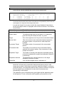
The user must specify the following information for fixed-schedule annealing:
• Number of Iterations
• Initial ‘Temperature’
• ‘Cooling Factor’
• Number of ‘Temperature’ decreases.
The algorithm chooses a Planning Unit at random and determines the change in
value to the system if the status of that planning unit were to change. A negative
change (which is good) is always accepted. A positive change is accepted only if
the Metropolis criteria (Kirkpatrick et al 1983) says so. This is:
Random(
)<e
− change
temperature
Here Random() is a uniform random number between zero and one - U(0,1).
When choosing the control parameters consider the following
information/restrictions.
• Number of Iterations: This will determine how long the program will take to
run. A higher value should give you a better answer.
• Initial ‘Temperature’: This should be high. It should be roughly the same size
as an initial bad choice. From a practical standpoint that doesn’t really help
and experimentation is needed. Setting this to a negative number will flag the
adaptive schedule.
• Cooling Factor: Every time the temperature decreases it does so by this
factor. It is a number between 0 and 1 and usually higher than 0.8. Again it is
largely guesswork to set it and it depends upon the number of temperature
decreases. Temperature decreases according to the formula:
Tnew = CoolFactor × Told
Where Tnew is the new temperature and Told the old temperature. Usually it is
best to work out what the desired final temperature should be and to work
backwards. The final temperature should be close to zero but higher as the
iterative improvement section acts as a temperature of zero.
• Number of decreases. If the number of iterations is greater than 0 then the
number of decreases should be less than or equal to the number of iterations.
I normally have used 100 temperature decreases which works well with the
29
cooling factor of 0.85 or 0.9 and initial temperature of 5 or 8. The program can
handle quite large numbers of decreases and it can be as high as the number
of iterations (but no higher). The ideal value is probably 10,000. If it is higher
then there can be round off error associated with multiplying the old
temperature with the cooling factor which means that the final temperature
might not be what is expected.
Annealing schedules are usually called ‘adaptive’ when the annealing
parameters are derived from the problem. The adaptive schedule in the program
samples the solution space a number of times to find the maximum positive
change and the minimum positive change to the value of the reserve (note that
negative changes are desirable). It does this by considering a relatively small
number of changes to the system (Number of Iterations / 100). It then sets the
target final temperature as the minimum positive (Ie least bad) change and the
maximum according to the formula :
Tinit = Min Change + 0.1 x (Max change - Min change)
The cooling factor is then derived so that this final temperature will be reached
at the end of the annealing schedule.
• To signal the use of the adaptive annealing schedule set initial temperature to
a negative number in the input parameter file, or click the appropriate box if
using InEdit.
• Because it uses trial runs it is slower than fixed schedule annealing. If the
verbosity is set to level 2 (“general progress”) or higher then the adaptive
initial temperature and cooling factor are printed. These can be used in later
runs as the input parameters to a fixed annealing schedule.
• Although the program will set its own value for the Cooling Factor the input
parameter file must contain a valid number for this factor or it will not work.
30
3 SETTING UP THE INPUT FILES
There are five input files required for Marxan to run. The most important one is
the input parameter file which controls the type of scenario in operation. The
others are the planning unit file, the conservation feature file, the conservation
feature distribution file, the optional block definition file and the optional boundary
length file. The last is important when spatial considerations such as boundary
length or clumping are to be used.
The planning unit file contains information for each planning unit. The
conservation feature contains information relating to each conservation feature,
primarily the representation requirements. The block definition file can be used to
set values for groups of conservation features. The conservation feature
distribution file contains the way in which each conservation feature is distributed
across the planning units in the system.
The input parameter file controls all of the main control aspects of Marxan. It
controls what types of algorithms are used and in what manner they are used.
The format of this file makes it easy to open up and read using text editors
although the software InEdit.exe, which is described in Appendix B will edit this
particular file in a user friendly windows environment.
Provision is made for Marxan to read in files which are in the old Spexan format.
This is done by passing the command line parameter ‘-o’ to the program, and is
described below.
The new file format is much more convenient and easy to use. All of the input
files (except the input parameter file) consist of a header line and a main body.
The header line is a list of variable names describing what is contained in each
column of the body of the file. The choice of variables is described in separate
sections below, they are always single word lower case names. The order of
these columns can be set by the user. The variables in a single line can be
separated by a wide variety of characters. They can be separated by whitespace such as tabs or spaces, which is the format which the old Spexan files
follow. Alternatively they can have any number or combination of the following
set of character: {,”’:;|_}. This allows the format that arcview can import/export
which is a header line of variable names surrounded by inverted commas and
separated by commas. It also allows as wide a variety as practical and a wider
variety than will ever probably be needed or desired.
3.1 Command Line Parameter
There are currently two possible command line parameters. ‘-o’ which stands for
old-style and the name of the input file. If the old style flag is set then Marxan
assumes that all file formats are in the old style and not in the styles described in
this document. The input file name has a default of ‘input.dat’ but any can be
used and sent in as a command line parameter.
Running the file in this way:
Marxan.exe
31
will make Marxan assume that all files are in the new style and that the input file
name is ‘input.dat’
Another example:
Marxan.exe -o Sample/input2.dat
Here Marxan will expect everything in the old style and the input data file will be
‘input2.dat’ in the ‘Sample’ directory.
3.2
Planning Unit File
The default name for this file is “PU.dat” it is a necessary file and Marxan will halt
with an error message if it is not present. This file contains all the information
related to planning units except for the distribution of conservation features
amongst the planning units (which is stored in the PU versus Conservation
Feature file).
The planning unit file consists of a header line plus a number of data lines. The
column headers can include: "id","cost","status","xloc","yloc". Note that these are
all lower-case letters with no punctuation, spaces or numerals.
The program will run even if some of these columns are not included. The “id”
column is the only one which is necessary, and every line must contain a unique
id, if there are duplicates then all but the last one will be ignored.. The cost and
status columns are not necessary and will revert to a default value of 1 and 0
respectively. The xloc and yloc columns are critical if there are spatial separation
requirements for any of the conservation features, otherwise they need not be
included. They describe a point location for that planning unit, the centroid of the
planning unit perhaps or some other sensible choice.
Variable Name
Default
Notes
id
Critical
The id number for this planning unit. It
must correspond to the planning unit
versus species matrix and the
boundary length file.
cost
1
The individual cost of each planning
unit.
status
0
whether pu is locked in or out of system
xloc
Critical for Separation
x co-ordinate of pu (central point?)
necessary if separation is to be used
yloc
Critical for Separation
y co-ordinate of pu (central point?)
necessary if separation is to be used
Most of these variables are well explained. The Status identifier can take one of
4 values. In general only values of 2 or 3 are useful.
Status
0
Meaning
The PU is not guaranteed to be in the initial or ‘seed’ reserve.
32
However it still may be. It’s chance of being included in the
initial reserve is exactly the ‘starting proportion’ from the
parameter input file.
1
The PU will be included in the ‘seed’ reserve or the initial
reserve. It may or may not be in the final reserve.
2
The PU is fixed in the reserve. It starts in the initial reserve and
cannot be removed.
3
The PU is fixed outside of the reserve. It is not included in the
initial reserve and cannot be added.
3.3
Conservation Feature File
This is a necessary file with a default name of ‘spec.dat’. If it is not present then
Marxan will halt with an error message. This file controls all the information for
each conservation feature, such as their targets, names and so forth. It does not
contain information on their distribution across planning units which is held in the
planning unit versus conservation feature file described below.
The Conservation Feature file (also known as the species file) contains
information on each of the conservation features under consideration. This file is
special in that not all the sets of data need to be present, if some are not
included then default values will take their place. Also for some columns a value
of -1 will indicate that the value for that specific conservation feature will be
determined later, either with a block definition for that conservation feature “type”
or will revert to the default. The block definitions are set in the block definition file
which is described below.
The column headers can include: "id", "type", "target", "spf", "target2",
"sepdistance", "sepnum" and "name". The header name must be exact, note that
all letters are lower case. The “name” column is special. It can contain spaces, or
even other column separators. Marxan uses the fact that this is the only variable
that doesn’t have numbers in it to allow it to read in a bunch of words as a single
variable. When this variable is read in it will replace any separators with a single
space, so it is wise to only separate words in the conservation feature’s name
with single spaces, otherwise the name could be subtly altered.
Be careful not to include more than one definition for each conservation feature
id. If there are any duplicates then all but the last one will be ignored.
Variable Name
Default Value
Notes/Description
id
critical
The id number of the conservation feature. It
must correspond to the planning unit versus
conservation feature file.
type
0
Type is a user defined type. It is used for ‘block
definitions’
target
0
The target amount for the conservation feature.
33
spf
0
The penalty factor for that conservation value
target2
0
Minimum clump size. If a clump of a number of
planning units with the given conservation feature
is below this size then it does not count toward
the target.
sepdistance
0
Minimum distance at which planning units
holding this conservation feature are considered
to be separated
sepnum
0
Target number of mutually separated planning
units in valid clumps
name
no_name
A name in words. Can include spaces, all words
in name must start with a letter.
targetocc
0
The number of occurrences of the conservation
feature required. This can be used in conjunction
with or instead of ‘target’.
3.4
Block Definition
This is an optional file and if a file name is not given or if the file name is ‘NULL’
then Marxan will not attempt to find a block definition file. The purpose of the
block definition file is to set variable values for groups of conservation features.
For a given ‘type’ of conservation feature a number of default attributes can be
set which all conservation features of that type will take as their own. In order for
this to have any effect the conservation feature file must have conservation
features of the given type with attributes set to ‘-1’, which means that they take
on the default value defined in this file or the preset default value for that
attribute.
This means that there are three ways a conservation feature can have an
attribute set. The attribute can take on the basic default value for that attribute
type, the attribute can take on the block definition default defined in this file, or
the conservation feature can have the attribute set in the conservation feature
file. This allows for quick and easy mass definitions which can still be over-ridden
in the conservation feature file for special conservation features.
The possible variable columns are "type", "target", "target2", "targetocc",
"sepnum", "sepdistance", "prop",”spf”. Any that are not defined for any of the
types returns the original default value. “prop” is special but all of the other
variables correspond to those described with the conservation feature file.
The “type” variable must be present. This sets the type for which all the other
variable definitions apply. If a species is of the same type and it has a negative
value for the variable then it will take on the value given in the block definition. If
more than one line is defined for a given type then each line will be applied for
this type starting with the last one encountered in the file and going backwards. It
is not recommended to have more than one line for any conservation feature
type.
34
A block definition for a type need not have values for all of the variables or
columns presented in this file. Set any variables to -1 which are not part of the
definition, then they will not replace the default value for that variable for species
of the same type.
“prop” is a special variable, short for proportion. This is the proportion of the total
amount for a species which is to be reserved. For example, a prop of 0.1 will set
a target of 10% of the total amount of that species based upon the PUvSPr.dat
data matrix. “Prop” replaces the target with this calculated value and will only do
so if there is no target definition for that species (Ie target has been set to -1). In
a block definition “target” and “prop” should not both be defined as they refer to
the same variable, albeit in differing ways. If they are both set then the “prop”
variable will take precedence and the “target” variable will be ignored in the block
definition. Also note that the proportion is based on the total amount defined in
the main species versus planning unit file. This might not be the same as the
total amount in the area, particularly if preprocessing of the data set has
occurred, for instance to remove occurrences of the conservation feature which
are fragmentary.
Variable Name
Default Value
Notes
type
Critical
The type for which the other attributes are
defined
target
-1
The target amount for the conservation
features of the given type.
target2
-1
Minimum clump size. If a clump of a
number of planning units with the given
conservation feature is below this size then
it does not count toward the target.
targetocc
-1
The number of occurrences of the
conservation feature required. This can be
used in conjunction with or instead of
‘target’.
sepnum
-1
Target number of mutually separated
planning units in valid clumps.
sepdistance
-1
Minimum distance at which planning units
holding the conservation feature are
considered to be separated.
prop
N/A
An alternative to target. This is the
proportion of the total amount of the
conservation feature which must be
preserved.
spf
-1
The penalty factor for that conservation
feature
35
Prop is not used if it is not present. Setting it to -1 (or any negative value) will
also ensure that it is not used. It makes sense to set prop to a number between 0
and 1. This is the proportion of the total amount of the given conservation feature
which must be included in the reserve system. It is used in place of ‘target’. For
example setting this to 0.05 would mean that 5% of the total amount available for
that conservation feature (including amounts in planning units which are locked
into or out of the reserve system) must appear in the solution. It is possible to set
this value higher than 1 just as it is possible to set ‘target’ to be higher than the
total amount available.
3.5
Boundary Length File
This file is optional and if no file name is provided or the file name ‘NULL’ is used
then Marxan will not attempt to load this file.
The Boundary Length file contains information on the boundary costs of adjacent
planning units. Whereas this cost is typically the actual length of the boundary it
can be modified to a ‘cost’ or ‘effective length’ value to take into account
boundaries which are particularly desirable or undesirable.
The boundary costs should always be 0 or positive values. A zero cost boundary
is useful only if some of the conservation features have a minimum clump size
(Ie target2 >0 for some conservation features) and you want to identify two of the
planning units as neighbours but there is no actual boundary cost.
The boundary length file starts with a header line which denote which column
has which meaning. The column identifiers are : "id1","id2","boundary". All three
identifiers are necessary.
id1 and id2 are the id numbers of two adjacent planning units. “boundary” is the
boundary length between them. It does not matter which order the id numbers
are entered but be careful not to duplicate boundaries because duplicates are
summed together.
There are two special types of boundaries, ‘free’ boundaries and ‘irremovable’
boundaries. A free boundary might occur where part of the perimeter of a
planning unit abuts an area which attracts no boundary penalty. For terrestrial
systems this might occur on the coastline. It is not necessary to include free
boundaries in the file. Irremovable boundaries occur where there is no possibility
of including a neighbour to the planning unit in the nature reserve, as on the
edge of the mapped system. An irremovable boundary is identified as a
boundary of a planning unit with itself. Ie the planning unit id number is repeated
twice for both id1 and id2.
Be careful not to duplicate boundary definitions. If two lines refer to the same two
planning units then their boundaries will be added together.
Variable Name
Default
Notes/Description
id1
critical
planning unit id
id2
critical
neighbouring planning unit id or the same as id1
for an irremovable boundary
36
boundary
3.6
critical
the boundary length
Planning Unit versus Conservation Feature File
This is a necessary file with a default name of ‘puvspr2.dat’. If it is not present
then Marxan will halt with an error message. This file contains the information on
the distribution of conservation features across the planning units.
There are two different formats which are acceptable for this file – the relational
format and the tabular format. Marxan will first test the header line to see if it is in
a relational format, if it is not it will try to process the file as a tabular format. This
means that the program need not be told which format is in use. It also means
that if the format is faulty than the error message which is produced might be
misleading.
3.6.1 Relation Format
The relational format for the planning unit versus conservation feature file starts
with a header line which denote which column has which meaning. The column
identifiers are : "species", "pu", "amount". All three identifiers are necessary.
“species” is the identification number of a species or conservation feature which
corresponds to the id in the conservation feature file.
“pu” is the planning unit id which corresponds to the id in the planning unit file
“amount” is the amount of that species or conservation feature which occurs on
the planning unit.
Variable Name
Default
Notes
species
critical
conservation feature id
pu
critical
planning unit id
amount
critical
amount of conservation feature on planning unit.
3.6.2 Tabular Format.
The tabular format for the planning unit versus conservation feature file is stricter
with regard to formatting. The header line consists of “pu” in the first column
followed by each of the species id numbers in turn. If any id number is repeated
then the later column will take precedence over the earlier column. If any id
number does not appear on the header line then the amounts for that species
will be zero for all planning units.
Each row represents the abundances (or occurrences) of conservation features
on a planning unit. The first column contains the planning unit numbers and the
other columns are the values for each conservation feature. If a planning unit id
appears on more than one row then the later row will over-write the contents of
37
earlier rows. If a planning unit does not have a row then there will be no
conservation features on it.
The conservation feature id numbers must correspond to id numbers in the
conservation feature file and the planning unit id numbers must correspond to id
number in the planning unit file.
3.7
Input Parameter File
This file contains all of the main parameter definitions to control the way in which
Marxan works. It is the file which will primarily be changed between each
scenario. This section describes the variables in the file and their default value
but does not describe in detail how to use these variables to control the flow of
the program. There is a graphics user interface for editing this file called
Inedit.exe and this is described in Appendix B. Reading the appendix rather than
this section is the easier way to learn about all of the parameters, particularly if
Inedit.exe is available and going to be used.
In the input parameter file, any line which does not start with one of the valid
variable names is ignored and hence can be used as a comment line. Note that
all of the variable names are single words in capital letters. Thus it is safe to start
a comment line with any word which is not all capitalised. A future version of the
program which might be able to accept different variables will not misread such a
comment line from an older input parameter file.
To set the value of a variable. Start a line with the variable name and follow it
with the value to set that variable to. Do not include any comments on the end of
the line, in case Marxan thinks that the comment is part of the variable value.
The variables can occur in any order in the file, but an error will result if any
variable is defined twice. Most of the variables have default values which will be
used if they are not defined.
The parameters in the input parameter file are as follows
Variable Name
VERSION
Default
Value
0.1
Description
Type of Input File
BLM
0
Boundary Length Modifier
PROP
0
Proportion of sites to start in run
NUMITNS
0
Number of iterations for annealing
STARTTEMP
1
Starting temperature for annealing
COOLFAC
0
Cooling factor for annealing
NUMTEMP
1
Number of temperature decreases for
annealing
RANDSEED
-1
random number seed
BESTSCORE
0
Kept for backward compatibility
COSTTHRESH
0
Cost Threshold
38
THRESHPEN1
0
Threshold penalty parameter 1
THRESHPEN2
0
Threshold penalty parameter 2
NUMREPS
1
Number of repeat runs
SAVERUN
0
Save each run?
SAVEBEST
0
Save best run?
SAVESUM
0
Save summary information?
SAVESCEN
0
Save Scenario information?
SAVETARGMET
0
Save targets met information?
SAVESUMSOLN
0
Save summary solution information?
SAVELOG
0
Save log file?
SAVESNAPSTEPS
0
Save Snapshots each n steps?
SAVESNAPCHANGES
0
Save snapshot each n changes?
SAVESNAPFREQUENCY
0
Frequency of snapshots if used.
temp
Scenario name for save files
INPUTDIR
Critical
Input directory for data files
OUTPUTDIR
Critical
output directory for saved files
SPECNAME
spec.dat
SCENNAME
PUNAME
PU.dat
name of species file
name of planning unit file
PUVSPRNAME
puvspr2.dat
BOUNDNAME
bound.dat
Name of boundary length file
gspec.dat
Name of block definition file
BLOCKDEFNAME
RUNMODE
Critical
Name of planning unit versus species
file
Run Mode
CLUMPTYPE
0
Clumping penalty type
MISSLEVEL
1
Level of target to be counted as missing
ITIMPTYPE
1
Iterative Improvement Type
HEURTYPE
1
Heuristic type
VERBOSITY
1
Verbose Mode
The most convenient way to edit this file is using the Inedit.exe program which is
purpose built to edit this file and is described in Appendix B. Although it may well
be useful to examine the file as a text file and alter it on occasion. If a Unix
version of Marxan were being used then Inedit.exe would not be as useful.
39
Here is a more detailed description of the variables. This is primarily for
reference, other sections examine the effects of these different variables and
sensible value choices.
Version Number. This is included to improve backward compatibility of
SPEXAN, it’s primary purpose is to allow Inedit.exe to read old input.dat files
automatically.
Boundary Length Modifier. This relates how the boundary length relates to the
cost of the system. How important is it to clump planning units together?
Boundary length might be measured in kilometres in which case this means the
dollar cost of each kilometre. Boundary length might already be given in a dollar
cost even without this modifier. BLM can be set to zero to remove the boundary
length cost.
Starting Proportion of Sites. The initial reserve can be anything. This is the
proportion of planning units which will be included. It must be a number between
0 and 1 where 0 means no P.U.s are included in the reserve, and 1 means they
all will be. Each planning unit has this number as a chance of being in it. Eg if the
number were 0.5 then each P.U. has a 50% chance of being included. This is
done before the planning unit status is included. So it is not, strictly speaking, the
expected proportion of planning units which will be in the initial reserve.
Initial temperature, cooling factor, iterations and number of temperature
decreases have all been described earlier in this document in the section on
Simulated Annealing.
Integer Random Number Seed.The random number seed must be an integer, if
it is negative then the clock is used to get a random seed. So if you don’t want to
repeat results exactly and you want to get new results without having to change
the seed then just set it to -1.
Best Score Hint. The system will keep track of the best reserve so far and will
eventually feed this into the iterative improvement routine. Because there is a
time cost involved in doing this and because the initial score might be ridiculously
high, I’ve included this value so that the algorithm will not start keeping track of
the best reserve until the reserve scores have reached a sensible number. This
is a time saving measure which is probably never required. It should be set a bit
higher than the expected best reserve value. If it is set to -1 then this feature will
be disabled.
Cost Threshold
This is the combined cost + modified boundary length
which a reserve can have without attracting a penalty . See the Inedit manual
(Appendix B) for more details. Setting the cost threshold to zero disables this
feature.
Threshold Penalty Factor ‘A’
The size control of the penalty curve. This
helps determine how large a penalty will be the final penalty. See the Inedit
manual (Appendix B) for more details.
40
Threshold Penalty Factor ‘B’
The shape control of the penalty curve. This
determines how gradually the penalty has an effect on the algorithm. See the
Inedit manual (Appendix B) for more details.
Number of repeats. Usually you would want to run the simulation a number of
times and see what the overall best result was. This is the number of repeats.
Each repeat is independent.
Save each run? Set this to 1 in order to save the final reserve from each run.
Setting this to 2 will save it in ArcView compatible text format (comma delimited
and with column headings).
Save best run? Set this to 1 in order to save the lowest scoring reserve from the
entire set of runs. Setting this to 2 will save it in ArcView compatible text format
(comma delimited and with column headings).
Save summary information? Set this to 1 to save a table of information giving
the details of the best reserve for each run. Setting this to 2 will save it in
ArcView compatible text format (comma delimited and with column headings).
Save scenario details? Set this to 1 to save the input parameters and other
fixed details to a file. Setting this to 2 will save it in ArcView compatible text
format (comma delimited and with column headings).
Save conservation feature targets met for each run? Set this to 1 to save the
number and a list of all conservation features which are not met by the best
reserve in the run for each run in the series. Setting this to 2 will save it in
ArcView compatible text format (comma delimited and with column headings).
Save Summed Solution? Set this to 1 to save the set of runs added together.
This file contains the number of times each planning unit occurred in a solution.
Setting this to 2 will save it in ArcView compatible text format (comma delimited
and with column headings).
Save Screen Log? Set this to 1or higher to save all of the screen output to file.
Save Snapshots each n steps? Set this to 1 or higher so that during the run
the current solution will be saved after the given number of steps. This is only
used with simulated annealing (there are other ways of producing similar
information with the other algorithms. The number of steps is determined by the
snapshot frequency. The file is called filename_snap_r1_t0001.dat (for the first
snapshot in the first run.). Setting this to 2 will save it in ArcView compatible
format (comma delimited and with column headings).
Save Snapshots each n changes? Set this to 1 or higher so that during the run
the current solution will be saved after the given number of changes to the
solution. This is only used with simulated annealing (there are other ways of
producing similar information with the other algorithms. The number of steps is
determined by the snapshot frequency. The file is called
filename_snap_r1_t0001.dat (for the first snapshot in the first run.). Setting this
41
to 2 will save it in ArcView compatible format (comma delimited and with column
headings).
Frequency of snapshots if used. This is the snapshot frequency which is used
only if snapshots are being saved. It is either the number of steps or the number
of changes between each snapshot, depending upon which option is active.
Scenario saving name. Each file will begin with this string. Appended to this will
be a suffix which depends upon the type of saved file. The suffixes are described
along with the saved files below.
Input directory name.
The name of the directory where all the input files
except this one are to be found. They must all be in the same directory as each
other. If this is left blank or given the value 0 then Marxan will assume that the
files occur in the same directory as itself.
Output directory name.
The name of the directory where any output files
are to be saved. If this is left blank or given the value 0 then Marxan will save
any output files to the same directory as itself.
Run mode. There are six run modes:
-1
Use no methods
0
Apply annealing and then the heuristic algorithm
1
Apply annealing followed by the iterative improvement algorithm
2
Apply annealing followed by the heuristic followed by iterative
improvement.
3
Use only the heuristic.
4
Use only iterative improvement
5
Use heuristic followed by iterative improvement.
6
Use only annealing
Clump Type. This is useful only if some species have minimum clump size
requirements (Target2). The clumping rules apply to all species with Target2 set
higher than 0. There are three options described in more detail in section1.2.5:
0
Step function. Small clumps score nothing.
1
2 level step function. Small clumps score half their amount.
2
Graduated. Scale is proportional to size of small clump.
Miss Level. This is the proportion of the target which a conservation feature
must reach in order for it not to be counted as missing. This should be between 0
and 1. Usually it would be set close to 1 maybe at 0.95 or higher. This allows the
missing values count to differentiate between those values which are arbitrarily
close to their targets and those which are significantly below them.
Iterative Improvement Type. There are four options. Iterative improvement will
only be used under some Run modes. These methods are described in detail in
Section 1.4.
0
Normal Improvement
1
Two Step Iterative Improvement
2
Swap Iterative Improvement
42
3
Normal followed by Two Step.
Heuristic Type. There are six heuristics which can be used. Under some Run
modes these heuristics are not used at all. Section 1.6 describes each of these
heuristic types.
0
Richness heuristic
1
Greedy Heuristic
2
Max Rarity
3
Best Rarity
4
Ave Rarity
5
Sum Rarity
7
Product Irreplaceability
8
Summation Irreplaceability
Verbose mode. The program likes to print stuff to the screen, the verbose mode
determines how much is dumped there.
0
Silent Running: The only output to the screen is the program
details.
1
Minimal output. It will show where it is up to and then the results
from each run and total run time.
2
Shows intermediate amount of detail
3
Shows exactly where the program is up to and gives the value of
the system every time the temperature changes. This is good for
long runs to make sure it is still thinking properly.
43
4
MARXAN OUTPUTS
Marxan can output both to the screen and to files. Often screen output is useful
to check on how the program is running and to give a quick summary of how
good the solutions are. The file outputs can be set to record much useful
information.
4.1
Screen Output
There are a number of levels of information that can be requested for screen
output. If the output level is set to anything more than ‘no output’ then summary
lines will be produced giving the value of the nature reserve system. These lines
might typically look like
Run 1 Value 1070.5 Cost 120.0 PUs 120 Boundary 350.0 Missing 2 Penalty 600.5
Run 1 indicates that this is the first run of the algorithm. The run number does
not always appear on the same line as the valuation of the reserve. It depends
upon the information detail level.
Value 1070.5. This is Spexan’s value for the reserve. It is the Cost plus the
Boundary value plus the Penalty for missing species. Because the penalty is
included in this Value the meaning of the value requires interpretation.
Cost 120.0. This is the cost for the reserve system. It is the sum of the costs of
all the Planning Units in the reserve system in the appropriate units of
measurement.
PUs 120. This is the number of Planning Units in the reserve system. In this
particular example the cost is equal to the number of Planning Units because
each Planning Unit has a cost of one.
Boundary 350.0. This is the boundary length for the reserve system.
Missing 2. This is the number of conservation feature which are underrepresented in the reserve system. This is screened according to the ‘miss level’
which has been set in input.dat. If the miss level is set to 1 then every
conservation feature which falls below its target level is counted. Often
conservation features can be very very close to the target level and it is desirable
to count these as not missing. In this circumstance the miss level can be set
below 1.
Penalty 600.5. This is the penalty for not representing all the species. If they are
all represented then it will be either 0.0 or -0.0. Because of round-off error it is
not likely to be exactly equal to zero but with only one decimal place presented
the round-off error will be well hidden. The penalty is roughly equal to the cost of
making up the shortfall of the species if it were possible to include partial
Planning Units and if there were enough of the species to make up the shortfall.
44
An information level of “General Progress” will include other information which
makes it a bit harder to read the bare results. This information includes the
successful loading of files and how many lines were successfully read, The score
of the reserve at different points in a run, and more time measures. When using
adaptive annealing with this level of information the calculated initial temperature
and decrement are also displayed.
This is the level which should be used when first setting things up. It allows the
designer to check that the files are loading correctly and that everything is
running smoothly.
The final information level of “Detailed Progress” is probably more detail than is
normally required. The most useful additional information that it gives out is the
order in which planning units are added when using heuristics and when using
simulated annealing it will print out the current reserve system score each time
the temperature is decremented.
This is useful for tuning a fixed schedule annealing run. You can see how it is
progressing and whether it is spending too much time at non-productive
temperatures and whether it is spending too much or too little time at low
temperatures.
4.2
File Output
There are seven types of file output that Marxan will currently allow. These are:
• Solutions for each run,
• Missing value information for each run,
• Best solutions of all runs,
• Summary information,
• Scenario details,
• Summed solutions over all runs,
• Screen log file,
• Snapshot files.
In each of the above except for summary information and the screen log file
there are two types of output, both are ascii text files. The first and standard
output has variables separated by tabs. The second includes column headings in
inverted commas and all variables separated by commas, this is the text format
which arcview expects and can import into a table.
The summary information and the screen log file are not tabular and are plain
ascii text.
The files each take on the scenario name as the first part of their file name and
then append a code depending upon what type of file it is.
45
4.2.1 Solutions for each run
A file is produced for each run of the algorithm containing the planning units
which constitute the final solution produced by that algorithm. These files take on
the names: scenario_r001.dat, scenario_r002.dat et cetera, where ‘scenario’ is
the name supplied by the designer.
The file consists of a list of planning unit ids which constitute the reserve. Each id
is on a new line. If the ArcView (or csv) format is chosen then a heading line with
“”planning unit”,”solution”” will also appear and each line will have the id number
followed by a 1 separated by commas.
4.2.2 Missing Values for each run
These files take on the names: scenario_m001.dat, …, scenario_mvbest.dat.
They contain information on how well the final reserve system from each run and
also the best run did with regard to meeting the conservation feature’s target.
This file will only be generated for solution files which are also generated. It must
be selected with either the solutions for each run option and or the best solution
option.
The old style file looks like:
Conservation Feature
Target
Target met
id number
Proportion of
value
target met
24
X
125.00
yes
1.29
161.00
23
W
170.00
yes
3.61
614.00
Here the first value is the conservation feature id number and the second is the
name as supplied in the species file. In this example the names are just single
letters. The target is the target amount for that conservation feature and the next
column contains either ‘yes’ or ‘no’ depending upon whether the reserve system
meets the target for that conservation feature. The next column is the proportion
of the target which was met which is the total amount of that species divided by
the target. The final column is the actual amount of that conservation feature
which appears in the reserve.
Because the new style allows for a more complex system of targets including
occurrence targets and variable separation requirements a new style of file was
required. This file can be in simple text format or in Arcview (csv) style. The
contents of the file are the same in both cases. In the text format style the
columns are separated by tabs and in the other style the columns are separated
by commas with inverted commas surrounding the column headers.
"Conservation Feature","Feature name","Target","Amount Held","Occurrence
Target ","Occurrences Held","Separation Target ","Separation
Achieved","Target Met"
24,X,0.000000,50.000000,0,5,0,0,yes
23,W,0.000000,187.000000,0,5,0,0,yes
46
22,V,0.000000,95.000000,0,5,0,0,yes
Arcview format. Comma separated with inverted commas delimiting text.
24
23
22
Conservation Feature
Feature Name
Occurrence Target
Occurrences Held
Separation Achieved
Target Met
X
0.000000
50.000000
0
5
W
0.000000
187.000000 0
5
V
0.000000
95.000000
0
5
Target
Amount Held
Separation Target
0
0
0
0
0
0
yes
yes
yes
Text format. Note that the first two lines in this table are not separated by a line break and
would appear on a single line if the margins were wider.
In a raw text format it is not easy to match the column headers to the columns,
but this can easily be done in a program such as Excel or Arcview. The columns
are as follows:
Column Name
Description.
Conservation Feature
The unique id number of the conservation feature
Feature Name
The optional string name for the feature. If no names are
given then they will all take the value ‘no_name’
Target
This is the target amount (if any) for the conservation feature
Amount Held
This is the amount of the conservation feature captured in
the reserve system. Only amounts in valid clumps are
included.
Occurrence Target
The target number of occurrences for the conservation
feature
Occurrences Held
The number of occurrences of the conservation feature
captured in the reserve system. Only occurrences in valid
clumps are included.
Separation Target
The number of mutually and adequately separated planning
units to be included which contain the conservation feature in
a valid clump.
Separation Achieved
The separation that is actually achieved, or the target
separation, whichever is lower.
Target Met
‘yes’ if all three targets are met, otherwise ‘no’.
Note that in all cases only conservation features and planning units in valid
clumps are counted. A valid clump is one which meets the ‘target2’ or minimum
clump size target. If a conservation feature does not have a minimum clump size
then the clump size is considered to be zero and all occurrences are
automatically in valid clumps.
The separation count of a species never goes higher that the separation target
for that species. This is a convention which speeds up the execution of the
47
software, but it means that no information is given about how far this target is
exceeded when it is exceeded.
The ‘proportion of target met’ column in the old style does not occur here,
although all of the information necessary to calculate proportions of target met
are.
4.2.3 Best Solution for all runs
This file is named scenario_best.dat, where scenario is the name the designer
supplied for the scenario. It contains the best solution from a set of runs. The file
consists of a list of planning unit ids which constitute the reserve. Each id is on a
new line.
4.2.4 Summary Information
This file is named scenario_sum.dat, where scenario is the name the designer
has given to the scenario. It contains summary information on each run with a
header line which describes what is in each line. A typical file looks like:
Run no.
Score
Cost
Planning Units
Boundary Length
Penalty
Shortfall Missing
Values
1
317.46
233.85
15
0.00
83.61
6.00
1
2
315.71
252.42
15
0.00
63.29
9.00
3
3
317.26
259.70
16
0.00
57.56
5.00
2
4
310.76
227.15
14
0.00
83.61
6.00
1
5
318.01
234.40
15
0.00
83.61
6.00
1
Most of the columns are self explanatory. Run No. is the run number for that line.
Score is the objective function score for the resulting reserve system. Cost is the
cost value for the resulting reserve system. Planning Units is the number of
planning units in the reserve system. Boundary Length is the unmodified
boundary length of the reserve system. Penalty is the penalty score for missing
conservation features for the reserve system. Shortfall is the shortfall of all the
conservation features which haven’t met their target. It is the sum, over all
conservation features, of zero if the conservation feature has met its target and
the amount by which the target hasn’t been met hasn’t. Missing Values is the
number of conservation features which haven’t met their target.
The last three columns are useful when there are some conservation features
which haven’t met their target, in determining how poor the reserve system
actually is. It is possible to have a high penalty and still be very close to the
targets, particularly if the conservation feature penalty factors have been set very
high. The shortfall is a good indication of whether the conservation features are
very close or very far from their targets and the number of missing conservation
features gives further information in this vein. If there are five conservation
features which each have missed their targets but the combined shortfall is very
small then they might all be at 99% or higher of targets and the designer might
not be particularly concerned.
48
4.2.5 Scenario Details
This file is named scenario_sen.dat, where scenario is the name the reserve
designer supplied. It contains a documented list of the options that made up that
scenario. Such a file may look like:
Number of Planning Units 99
Number of Conservation Features 24
Starting proportion 0.00
Boundary length modifier 0.00
Algorithm Used :Annealing and Iterative Improvement
No Heuristic used
Number of iterations 100000
Initial temperature 1.00
Cooling factor 0.999550
Number of temperature decreases 10000
Cost Threshold Disabled
Threshold penalty factor A N/A
Threshold penalty factor B N/A
Random Seed -1
Number of runs 10
The file is relatively self explanatory. Its use is to keep track of scenario details
when multiple scenarios are run.
4.2.6 Summed Solution
One option in Marxan is to add all of the solutions from a run together. What this
does is keep track of how often each planning unit was involved in any solution.
This information is a useful way to explore the irreplaceability of planning units.
The file is named scenario_ssoln.dat where scenario is the designer supplied
name for that scenario.
Each line has the id number of a planning unit and the number of times that that
planning unit was involved in a solution.
4.2.7 Screen log file
With this option all of the screen output is also saved to a file. The file is named
scenario_log.dat where scenario is the designer supplied name of the scenario.
Because the information is a copy of that which is presented to the screen the
level of information is controlled by the verbosity level.
4.2.8 Snapshot file
With this option the state of the solution is saved routinely during some of the
optimisation methods. The solution is saved in the save format as the final
solution for each run or the final best solution (see section 4.2.1).
This option allows the user to examine the progress of a solution method,
although the user will have to find a suitable method for examining these
solutions (using either another program such as ArcView or Excel).
49
There are two options for saving ‘snapshots’ these are the ‘each n steps’ or
‘each n changes’ methods. The first saves the state of the system after the
specified number of steps. The other saves the state of the system after it has
been changed the specified number of times.
The name of the file for the snapshots can be convoluted, particularly if there are
th
many repeats. For example scenario_snapsc09999.txt is the 9999 snapshot
after ‘n’ changes when there is no repeat. If this were the third repeat then it
th
would have been scenario_snap_r00003sc09999.txt. If it were the 800
snapshot after ‘n’ iterations then this would be
scenario_snap_r00003st00800.txt.
50
REFERENCES
Ball, I., R., Smith, A., Day, J. R., Pressey, R. L. and Possingham, H., P (In Press) “Comparison
of Mathematical Algorithms for the Design of a Reserve System for Nature Conservation: An
Application of Genetic Algorithms and Simulated Annealing.” Journal of Environmental
Management
Connolly, D. J. (1990) “an improved annealing scheme for QAP”, European Journal of Operations
Research, 46, 93-100.
JANIS (1997) Nationally agreed criteria for the establishment of a comprehensive, adequate and
representative reserve system for forests in Australia. A report by the Joint ANZECC/MCFFA
National Forest Policy Statement Implementation Subcommittee. National forest conservation
reserves: Commonwealth proposed criteria. Commonwealth of Australia, Canberra.
Kirkpatrick, S., Gelatt jr, C. D., and Vecchi, M. P. (1983) Optimization by Simulated Annealing.
Science, 220, 671-680.
Possingham, H., Ball, I. R., Andelman, S. (2000) “Mathematical methods for identifying
representative reserve networks” in Quantitative methods for conservation biology. Ferson, S.,
and Burgman, M. (eds). Springer-Verlag, New York.
Pressey, R. L., Humphries, C. J., Margules, C. R., Vane-Wright, R. I., and Williams, P. H., (1993)
“Beyond opportunism: Key principles for systematic reserve selection”, TREE, 8, 124-128
Pressey, R. L., Johnson, I. R., and Wilson, P. D., (1994) “Shades of irreplaceability: towards a
measure of the contribution of sites to a reservation goal.”
Pressey, R. L., Possingham, H. P., Margules, C. R., (1996) “Optimality in Reserve Selection
Algorithms: When Does it Matter and How Much?” Biological Conservation 76, 259-267.
51
Appendix A: History of changes to Marxan
Differences between version 1.7 and 1.6
A new file format for the PU versus CF file is allowable. This is the tabular format
in which each row represents the distribution of species on a planning unit and
each column the distribution of a species across planning units.
Marxan will assume that the normal style is in use unless the header line is not
correctly formatted for that file. In this case it will assume that the file is in the
new format and if it is not then it will print an error message and terminate.
This option is described in Section 3.6.2
New iterative improvement methods. There are now four variations on the
iterative improvement algorithm. These are: Normal iterative improvement,
‘Swap method’, ‘Two Step’ method or running normal iterative improvement
followed by ‘two step’. These options are described in Section 1.4.
Differences between version 1.6 and 1.2
A number of features have been added to Marxan since version 1.2 and these
are described in detail within this manual. This section has been added to make
it easy to see at a glance what the new features are.
•
New missing conservation feature output file. Described in Section 4.2.2, the
new output file contains information on the new target types supported in
Marxan, primarily the separation distance targets.
•
Screen Log File. Described in Section 4.2.7. This is an ascii text file in which
all the output to the screen is saved also to disk.
•
New penalty system for partial clumps. This is yet to be described within this
manual.
Differences Between Marxan and Spexan
Spexan is a terrestrial reserve siting optimiser written in c and based on an
earlier version Siman written in Fortran. Marxan is similar to Spexan from which it
grew. It is based on Spexan but with a few significant differences and
improvements.
• Input file directory now supports extended file and directory names.
• New improved file input system. Old style inputs still available
• Self annotated parameter input file.
• New file system allows any type of separator and columns in any order
• New file system has meaningful column names for ease of understanding
52
• New output option: Arcview compatible outputs for most output files
• New output file: Summed solution. Can now add up many solutions and
present combined solutions.
• New Block definition input file. Targets of any type can be given for groups of
species by changing a single number in the input file.
• New target type: TargetOcc. The number of occurrences needed for a given
conservation feature can replace or be used in conjunction with the normal
amount type of target. Works in conjunction with the minimum clump size
(target2) consistently.
• New target type: Prop. Can now specify a proportion of the total amount of a
conservation feature as the target for that conservation feature.
• Improved Spatial requirements. There is now no limit on the target separation
count for a conservation feature.
53
Appendix B: Using Inedit.Exe
Inedit.exe is a stand alone windows program which is designed to make editing
the input file for Marxan very easy. The program must be run from the same
directory as the input parameter file. When running the program click the ‘load’
button to load the input parameter file and click save to save your options.
It is presented as a tabbed notebook and each section is examined here
separately.
Problem
This section contains some basic problem definition information including the
proportion of planning units to start with and the boundary length multiplier.
Repeat Runs This is the number of separate runs with the same starting
conditions which will occur in one implementation of the program.
Boundary Length MultiplierThis is the scaling factor between boundary length
and planning unit costs. It can be any real value although it only makes sense for
this to be positive or zero. A quick way to remove boundary lengths from
consideration is to set this to zero. The program will still calculate information
based on the boundary lengths but this information will not be used.
Input File Type
Choose between the old style file type where the variable
is determined by the position in the file (which is compatible with Spexan) and
54
the new file type with variable names and comments which contains all the
options required for Marxan.
Run Options
This page covers both the starting proportion of planning units as well as options
governing the use of iterative improvement and heuristics. It is from this page
that the annealing module and the heuristics module can be turned on or off.
Run Options There are three modules which can act upon the reserve; they
occur, if at all, in a set order. The first is the simulated annealing module the
second is the heuristics module and the third is the iterative improvement
module. Iterative improvement ensures (if it is being used) that the resultant
reserve is a local minimum. All three modules can either be turned on or off and
this gives 6 possible run options. It is probably most sensible to follow simulated
annealing with iterative improvement only. Setting Heuristic only will test a
heuristic and you can follow it with iterative improvement to possibly improve it.
Running Iterative Improvement on it’s own will give a very poor solution (in
general) but could provide a baseline which any heuristic should beat.
Heuristic Type
This allows the user to set which heuristic is being used.
There are a number of different heuristics to chose from, they are described in
some detail in the spexan users manual. The heuristic will only actually be used
under certain run options.
55
Annealing
This page holds all the information needed to control the annealing regime.
Number of Iterations
This will determine the total number of attempted
changes during the annealing process. It must be positive and it is the main
factor which determines how long each annealing run will take.
Initial Temperature This must be a value greater than 0. It is worthwhile to set
a high initial temperature although the exact value depends upon the problem.
Adaptive Annealing (see below) can be used to generate a suggestion as to a
good initial temperature to try.
Cooling Factor
This determines how quickly the system cools. Rather than
setting it manually you can click on the option to ‘Set Cooling from Final
Temperature’ which is a much easier way to proceed and is the recommended
method.
Number of Temperature Decreases
This must be less than or equal to
the number of iterations. The higher the value the smoother the annealing will
be. I’ve found a value of 10,000 to be adequate for annealing. Setting it lower
can make the regime too coarse, setting it too high will lead to round-off error
problems with the temperature.
Setting Cooling from Final Temperature If this is selected then you can enter
a target final temperature (which must be higher than 0) and the appropriate
cooling factor will be calculated. By running an Adaptive Annealing regime (see
below) a good starting point for setting the final temperature can be obtained.
56
Adaptive Annealing Schedule
Selecting this will disable the Initial
temperature and cooling factor. These will be set by the computer instead. This
is done by making a trial number of changes and examining the best and worst
change values which result. The Initial and Final temperatures are derived from
this and are displayed by Spexan if the verbose level is set to ‘general progress’
or higher (see below).
Input
Species File Name The file name (with extension) of the conservation feature
(or species) file. This must be located in the input directory.
Planning Unit File Name
The file name (with extension) of the planning unit
file. This must be located in the input directory.
Planning Unit Versus Species File Name The file name (with extension) of the
planning unit versus conservation feature file name. It must be located in the
input directory.
Block Definitions
The file name (with extension) of the block definition file.
This must be located in the input directory. This is not a necessary file. If it is not
needed then turn off the checkbox or set the name of the file to NULL. If the
name is set to NULL then Marxan will not try to open the file.
Boundary Length
The file name (with extension) of the boundary length file.
This must be located in the input directory. This is not a necessary file. If it is not
needed then turn off the checkbox or set the name of the file to NULL. If the
name is set to NULL then Marxan will not try to open the file.
57
Input directory
This directory should be no longer than 80 characters in
length. It is the directory where every file except the input parameter file is to be
found.
Output
This screen controls the output options. This includes both the output to the
screen and the output to a file.
Screen Output
This determines how much information is displayed on the
screen. If you are saving the best solutions this could be set to ‘none’ (The title of
the program is still displayed). Setting it to ‘results only’ is usually worthwhile to
get the summary lines from each run. ‘General progress’ will display information
on what has been read in as well as details on any conservation features who’s
targets and requirements are such that they cannot be adequately reserved in
the system. The highest level is ‘detailed progress’ which can give you a good
feeling for how the annealing module is working (when it is being used).
Save Files
There are a six different types of file which can be saved when
running the algorithm. These are described below. Select some, all or none of
these files by checking or unchecking them.
58
Save Each Run
Each run is saved as a separate file named
filename_r1.dat, filename_r2.dat … where filename is the name supplied by the
user (see below). Each file consists of a list of planning unit numbers which
make up the best solution for each run.
Save Overall Best Save in the name filename_best.dat this is the best
solution from the series of runs.
Save Summary
This will save the summary of the runs in a file names
filename_sum.dat. Each line containing the results from a single run.
Save Scenario Details
Saved in the file filename_sen.dat are all the
details of the scenario, including the random seed which was used.
Save Missing Value Information names filename_t1.dat, ..l filename_tn.dat.
This lists how successful each solution was in meeting the targets for each
conservation feature.
Save File Name
This is the kernal for the names of all the files, the
filename of the six files listed above.
Do Not Count Species
This is the proportional cutoff for each conservation
feature, above which it is counted as having met the target. It is a proportion of
the target and is useful for the case where solutions are often sufficiently close to
their targets without actually meeting them. The value does not effect how the
algorithms run. A value of 1 will mean that this has no effect. If the value is lower
than 0.9 then it is worth considering changing the targets of the conservation
features.
Output directory This directory should be no longer than 80 characters in
length. It is the directory where any saved files will be placed.
59
Cost Threshold
The cost threshold is an option which allows the user to cap the reserve system
to a set cost + modified boundary length. It works by applying a penalty if the
given threshold value is exceeded. The penalty is the amount by which the
threshold is exceeded multiplied by the cost threshold penalty. The penalty
depends upon the stage of the annealing algorithm (how far into the annealing
process the system is given as a proportion). The multiplier is:
Cost Threshold Penalty = Amount over Threshold × ( Ae bt − A) .
Here t is the time during the run and varies between 0 and 1. A and B are control
parameters. B controls how steep the curve is (A high B will have the multiplier
varying little until late in the run). A controls the final value. A high A will penalise
any excess of the threshold greatly, a lower A might allow the threshold to be
slightly exceeded. The multiplier starts at 0 when t is zero. Both A and B require
some experimentation to set.
The cost threshold penalty is built into the objective function and hence will apply
to the annealing module along with the iterative improvement module and also
the heuristics module if the greedy heuristic is being used. It would be ignored by
the richness heuristic.
Cost Threshold Enabled
This must be turned on to use the cost threshold.
The cost threshold is a threshold value for the cost of a reserve system (cost +
modified boundary length).
Cost Threshold
This is the combined cost + modified boundary length
which a reserve can have without attracting a penalty .
60
Threshold Penalty Factor ‘A’
The size control of the penalty curve. This
helps determine how large a penalty will be the final penalty.
Threshold Penalty Factor ‘B’
The shape control of the penalty curve. This
determines how gradually the penalty has an effect on the algorithm.
Misc
These are the controls which did not easily fall into any of the above categories.
Starting Proportion This must be between 0 and 1. This is the proportion of
Planning Units which have a pre-defined status of 0 which are to form the initial
reserve. Note that in the planning unit file you can set the status of each P.U. as
either 0 (= not currently in reserve), 1 (= currently in the reserve), 2 ( = in the
reserve and not removable) or 3 (= not in the reserve and not available to be
reserved). All P.U.s with a status of 1, 2 or 3 will not be affected by the starting
proportion. Setting the starting proportion to 0 will mean that no new PU’s are
added to the initial reserve setting it to 1 will mean that every available P.U. is in
the initial reserve.
Random Seed
Set this to -1 if you want each application of the program
to be different or to any positive integer if you want to repeat your pseudorandom numbers. It should be set to -1 except for debugging purposes.
Output Saving
This is not a useful parameter. Set this value to -1, or click
off the check box. It is included for future versions of the program if run time
becomes a serious concern.
61
Appendix C: Old Style File Formats
General
If a command line parameter of -o is used then Marxan will be able to read files
in the old format. This is the format which was used by Spexan. If this option is
selected then most of the new features of Marxan will be unavailable. In this
appendix the old format specifications are given.
Input Files
There are a fair number of input files required. They must all be placed in a
directory named in input.dat (see below) and their names must be identical to
those given in the following table. If input.dat is not placed in the same directory
as Marxan then it’s name and location must be specified on the command line
when activating Marxan (see below).
Not all of these files are critical. If a non-critical file is missing then Marxan will
still run. The action that it will take depends upon the file and are described in
their respective sections. The non-critical files are the cost.dat file, pustat.dat,
puvsp.dat (in which case puvspr.dat is required), bound.dat, puxy.dat. The full list
of files is:
•
•
•
•
•
•
•
•
•
input.dat Controls all the input options
cost.dat The (fixed) cost of each planning unit
species.dat
All the important conservation feature specific pieces of
information.
bound.dat
information on cost of boundaries and also number of neighbours
pustat.dat
P.U. status data. Are planning units already in the system? Are
they removable?
puvsp.dat
P.U. versus conservation feature data. The amount of each
conservation feature on each planning unit.
puvspr.dat
An alternative to puvsp.dat. This contains the amount of
conservations values on each planning unit in a different format to puvsp.dat.
puxy.dat The x,y co-ordinates for the Planning Units.
name.dat
The user defined identification numbers of the Planning Units.
input.dat
This is the most important file as it contains all the control instructions. The user
might well wish to alter it between each run. It is composed of numbers, one per
line, each one being an instruction in fixed order. The easiest way to edit this file
is to use the application inedit.exe (described in Appendix B). The default is for
this file to be named ‘input.dat’ and to be in the same directory as Marxan.
Alternatively a different directory and different filename can be specified on the
command line when Marxan Spexan. The command might be:
spexan c:\users\susan\games\doom\test.dat
62
Here the test.dat file must exist and be in the directory named and follow the
format given below.
The input.dat file should be constructed with the following information:
Double
Double
Double
Integer
Double
Double
Integer
Integer
Double
Integer
Double
Double
Integer
Integer
Integer
Integer
Integer
Integer
Integer
String
String
String
Integer
Double
Integer
Integer
Version Number
Boundary Length Modifier
Starting Proportion of Planning Units in the system
Number of Iterations
Starting Temperature
Cooling Factor
Number of Temperature regimes
Integer random number seed
Best Score hint
Cost Threshold
Threshold Penalty Factor 1
Threshold Penalty Factor 2
Number of repeats
Save each run? (0 for no)
Save best run? (0 for no)
Save Summary information? (0 for no)
Save Scenario details? (0 for no)
Save Conservation Feature targets met for each run? (0 for no)
Save Summed Solution? (0 for no)
Scenario Saving Name (no longer than 80 characters)
Input directory name (no longer than 80 characters)
Output directory name (no longer than 80 characters)
Run mode
Miss Level
Heuristic Type
Verbose mode.
Here Double is a ‘double-precision’ floating point number such as 3.141526928.
The file should end with a new-line, any extra lines below the final are ignored.
The order of variables is precise. It cannot be changed and on each line must be
a variable value of the appropriate type. The definition of each of these variables
is given in the main body of this document, they are identical to the new style
format.
Cost.dat
The cost of each planning unit. On each line of this file should be two numbers.
P.U. IDCost
The Planning Unit ID is the planning unit’s number. The cost is measured in any
units that you like. Missing conservation feature’s penalties will be in the same
63
units and it is up to the user to ensure that the units work with whatever is used
in the boundary length/cost file.
The order of planning units is irrelevant for this file. Any planning unit which has
no cost associated with it defaults to a cost of zero. If a planning unit is listed
twice or more then the costs are added up for this planning unit.
If Cost.dat is not present then every Planning Unit is given an identical cost of
1.0.
Species.dat
Each line has information for a different conservation feature. The conservation
feature must be in order. The following is required on each line:
Conservation Feature ID
Distance
Name
Category
Target SPF Target2 Separation
Conservation feature ID is the user supplied number of the value. This must be
an integer and must be unique. Spexan does not check that each value is unique
and strange things might happen if an ID number is repeated.
Conservation category is normally 1 for old growth 2 for forest ecosystem 3 for
flora or 4 for fauna. This is currently not used.
Target is the target for that conservation feature, either area or whatever
measurement you like.
Conservation feature SPF is the Species Penalty Factor also written as CFPF for
conservation feature penalty factor. It should be the same for most values and
lower for those you don’t really care about. There is no good theory at the
moment about what level achieves what effect. Setting it higher than 1 will
increase the motivation for the system to perfectly represent that conservation
feature.
Target2 is used if the species has a minimum clump size. This is the minimum
size of a clump which will count towards the target total. A clump is any number
(1 or more) of contiguous patches which contain this conservation feature. If it is
set to 0 then no aggregation is applied to this conservation feature.
Separation Distance is used when the conservation feature needs to exist in
patches separated by a given distance. This might occur when you want to
decrease the amount of damage caused to a conservation feature by a localised
catastrophe. If the separation distance is set to zero then this conservation
feature is not subject to a separation rule. If no conservation features have a
separation distance greater than zero then the file puxy.dat is not necessary,
otherwise it is crucial. The units for separation distance must be the same as
those used in puxy.dat.
64
Name. The name is a single word for the conservation feature and can be
anything. It is used when generating the ‘missing value’ report file and also for
certain screen output information when the screen output setting is set to
‘detailed’. This name must not contain spaces and must be shorter than 200
characters in length.
Bound.dat
This file need not be included if boundaries are not important to your reserve.
Each line has a cost and two Planning Unit numbers (Which is their order in the
list starting from 0 and going up to 1 less than the number of planning units. The
cost or length is the cost of the boundary between the two planning units named.
The cost can be zero if you want to mention that two planning units border each
other but there is no cost for the border.
Some planning units might have a fixed border cost (maybe they are on the edge
of the system). In this case give the fixed cost and then repeat the number of the
planning unit. For example:
5.0 10 10
means that planning unit 10 has a non-removable border cost of 5.0.
Because the boundary is always multiplied by the boundary length modifier it
doesn’t matter what units are used in this file.
Multiple boundary definitions are dangerous and should be avoided. If a there is
more than one fixed boundary cost for a given planning unit then these costs are
added together. This might be useful for certain geometric shapes where the
fixed costs refer to different segments of the boundary. Where there is more
than one boundary cost given for any two planning units then the second and
subsequent ones are ignored, although the fact that they exist is reported when
the verbose setting is 2 or more.
Pustat.dat
The status of each planning unit. Each line has two numbers
Planning Unit ID
Status Identifier
The Planning Unit ID is the user supplied ID number of the planning unit. These
lines can be in any order. The status identifier is 0 if the planning unit is not
currently in the reserve system and 1 if it is. Any other number might well be
used as if it were a 1. If a planning unit is not mentioned in this file then the
default value is 0.
Status Identifier and what the program does with it:
65
Status 0
The PU is not guarranteed to be in the initial or ‘seed’
reserve. However it still may be. It’s chance of being included in the initial
reserve is exactly the ‘starting proportion’ from input.dat.
Status 1
The PU will be included in the ‘seed’ reserve or the initial
reserve. It may or may not be in the final reserve.
Status 2
The PU is fixed in the reserve. It starts in the initial reserve
and cannot be removed.
Status 3
The PU is fixed outside of the reserve. It is not included in
the initial reserve and cannot be added.
If this file is not included then every planning unit is assumed to have a status of
0. If a planning unit is listed more than once then the last one in the file takes
effect. The fact that there are duplicates is reported.
PUvSP.dat
st
This file consists of a large matrix in which the 1 row of this file is the ID number
st
of each conservation feature. The 1 column is the ID number of each planning
unit. The cells of the matrix is the amount of that conservation feature on that
planning unit. The first cell (column 1 and row 1) should be left blank.
Use a value of 0 if the conservation feature is not on the given planning unit,
otherwise the level at which it is represented. This is a linear measure such as
hectares or populations. The units should be roughly equivalent for each of the
conservation features.
If this file is not present then the program will look for the file PUvSPr.dat
PUvSPr.dat
Optional file. If PUvSP.dat is not found then Spexan will look for this one. There
must be one of the two files or the program will abort. The file contains an
arbitrary number of records each line consisting of three numbers.
PU ID Conservation Feature ID
Amount
where Amount is the amount of the conservation feature appearing on that
Planning Unit. There is no checking for double entries, newer entries would
overwrite older ones.
PUXY.dat
This is an optional file but it is necessary if any conservation feature has a
separation distance greater than 0. It is the x,y location of each planning unit.
Each line should consist of three numbers.
PU ID X Loc Y Loc
These lines can be in any order. If there are more than one entry for a given
Planning Unit then the newer one will over-write the older and if any Planning
Unit does not have an entry then it’s X and Y location will both be set to zero.
The X and Y location can be in any distance measuring units but they must be
66
the same as the separation distances given in the file Species.dat. There is no
checking for double entries, newer entries would overwrite older ones.
name.dat
This file contains the user supplied identification numbers for each planning unit.
Each line must contain a single unique integer for one planning unit. Every
planning unit must have a line devoted to it. This file is compulsory.
67
Index
A
adaptive annealing schedule, 19
arcview, 31
Average Rarity, 24
B
Basic Concepts, 8
Best Rarity, 23
Best Solution for all runs, 47
BLM, 10, 13, 26, 38, 40
Block Definition, 34, 55
BLOCKDEFNAME, 39
Bound.dat, 63
boundary length, 10, 11, 12, 13, 16, 21, 23, 27, 31, 32,
36, 39, 40, 43, 47, 52, 55, 58, 62, 63
Boundary Length File, 36
BOUNDNAME, 39
input.dat, 26, 31, 32, 39, 43, 60, 61, 63
INPUTDIR, 39
irreplaceability, 6, 21, 24, 48, 49
Iterative improvement, 17, 28, 53
M
Maximum Rarity, 22
Missing Values for each run, 45
MISSLEVEL, 39
N
name.dat, 60, 65
NUMITNS, 38
NUMREPS, 39
NUMTEMP, 38
O
OUTPUTDIR, 39
C
Command Line, 31
Conservation Value File, 33, 37
conservation value penalty, 10, 12, 13, 14, 16, 22, 27,
47
COOLFAC, 38
Cooling Factor, 29
cost threshold, 10, 16, 26, 27, 40, 58
cost threshold penalty, 10, 16, 58
Cost.dat, 61
COSTTHRESH, 38
CFPF, 10, 14, 16
E
P
Planning Unit File, 32, 55
Product Irreplaceability, 24
prop, 20, 28, 29, 30, 32, 34, 35, 40, 42, 43, 45, 47, 49,
51, 52, 53, 54, 57, 58, 59, 61, 63
PROP, 38
PUNAME, 39
pure greedy, 22
Pustat.dat, 63
PUvSP.dat, 64
PUvSPr.dat, 64
PUVSPRNAME, 39
PUXY.dat, 64
economic costs, 10
R
F
fixed schedule annealing, 19
G
RANDSEED, 38
rarity algorithms, 22
References, 49
Richness, 21
RUNMODE, 39
greedy algorithm, 9, 12, 13, 22
Greedy heuristics, 21
S
H
HEURTYPE, 39
I
Inedit.exe, 27, 28, 31, 39, 52
Input Parameter File, 38
SAVEBEST, 39
SAVERUN, 39
SAVESUM, 39
Scenario Details, 47
SCENNAME, 39
Screen Output, 43
separation requirement, 11
separation rule, 14, 15, 62
sepdistance, 33, 34, 35
68
sepnum, 33, 34, 35
Setting the Scenario, 26
SIMAN, 8
Simulated annealing, 8, 9, 17, 18, 19, 20, 22, 28, 44,
53
Solutions for each run, 44
spatial aggregation, 14
Species.dat, 62
SPECNAME, 39
Spexan, 2, 6, 7, 8, 31, 43, 50, 52, 55, 60, 62, 64
spf (see also CFPF) , 33, 34, 35
STARTTEMP, 38
Summary Information, 47
Summed Irreplaceability, 24
Summed Rarity, 23
Summed Solution, 48
T
target2, 33, 34, 35, 36, 51
targetocc, 34, 35
The Objective Function, 9
THRESHPEN1, 38
THRESHPEN2, 38
V
VERBOSITY, 39
2