Download Antenna Network & Measurement Simulator

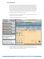
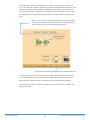
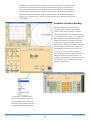
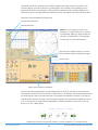
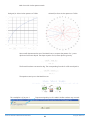
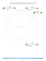
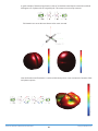
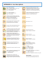
Antenna Network & Measurement Simulator
Users Manual
http://www.DiamondEng.net · [email protected]
P.O. Box 2037 Diamond Springs, CA 95619 · 530-626-3857
Antenna Network & Measurement Simulator
Diamond Engineering’s Antenna Network And Measurement Simulator is a
2-port vector cascade simulator specifically designed as a measurement and
processing tool. The simulator can simulate measurement results including noise
and phase. It can perform gain transfer functions, Radar Cross-section, Match
and antenna rotation & translation and circuit element implementations. It is an
icon based schematic capture simulator. It is not intended to replace high end
simulators but provides a simple intuitive tool in the DAMs software toolbox.
This manual will fully assist you in the use and application of the Simulator,
limitations and general considerations. It is assumed the user has at least a basic
network simulation knowledge. Pre-configured schematics with application
exploitations are included in this manual and with the software.
Best Regards,
The Diamond Engineering Team
Table of Contents
Simulator Overview..............................................................................................................................7
Benefits of Simulation.........................................................................................................................8
Introduction............................................................................................................................................9
Creating Branches and Parallel Networks...................................................................................18
Simple Antenna Measurement........................................................................................................19
Making Schematic Measurements.................................................................................................22
Using the Math Icon............................................................................................................................22
Using the Translation Icon.................................................................................................................26
Using the Rotation Icon......................................................................................................................29
Processing RCS Time Domain Measurement.............................................................................31
Using The Time Domain Icon...........................................................................................................36
APPENDIX A: Icon Descriptions...................................................................................................38
APPENDIX B: Scientific Calculator Overview..........................................................................39
APPENDIX C: Scientific Calculator Examples..........................................................................40
APPENDIX D: Exporting .S1P files...............................................................................................46
http://www.DiamondEng.net · [email protected]
P.O. Box 2037 Diamond Springs, CA 95619 · 530-626-3857
Simulator Overview
Overview
The simulator is a two port cascade S-parameter engine which uses icon based elements and
drag & drop workspace. When the DAMs measurement system performs a measurement one of 4
s-parameters are stored into the default display register (Reg0). A two port measurement consists of
4 s-parameters. The DAMs measurement software can produce all 4 s-parameters in individual Regs.
The simulator can make use of the individual measured [S] data and recombine it as necessary.
Important: There are 91 IconS available. Each Icon has 4 copies. Some have more and some have
less. A large cascade can be performed in sections and outputting each section to a storage Reg. See
Appendix A for Icon info.
Hides Calculator or Schematic
Initiates the simulator
Standard
Icons
Exports results as S1P files
Changes a series element
to a parallel element
Initiates analysis
Special function icons
Saves schematic and
all values to file
Initiates the scientific
array calculator
Clears or recalls
schematic. Double
clicking loads last
Loads schematic files
schematic after CLR.
Initiates the monitor plot Single click at start
and the array calculator up loads the last
present schematic.
Benefits of Simulation
The Antenna Network & Measurement Simulator module enables DAMS Antenna Measurement Studio
to perform a whole host of simulation capabilities. It’s designed to be fully customizable with drag-ndrop icon-based schematics which utilize capture vectors (cascading two-port with wave addition). Also
includes many other features such as circuit matching, radar cross-section, axis translation and rotation,
among others.
Drag & Drop Elements
Modify each icon location and it’s various properties
quickly and easily, ensuring accurate simulation.
RCS Profiling
Whether it’s a single object or an entire antenna
array—our simulator can accurately measure their
radar cross-section profiles.
RCS Color Map
dBSm
Perform Schematic Measurements
Design your own icon-based schematic to produce
accurate measurements or simulations in frequency
or time domain.
Easy To Use
Even though it is designed to be completely selfintuitive, we also offer all customers personal
assistance in order to help make simulations or
measurements as painless and accurate as possible.
Efficiency Saves Money
By using our simulator, you can design and measure
your own antennas or network devices in-house,
quickly and efficiently.
Analyze Network Path & Phase
Our simulator can help determine the proper path
alignment of a microwave antenna, which is crucial to
good signal reception.
Simulate Phased or Sector Arrays
Measure a group of multiple active antennas coupled
to a common source or load to examine the directive
radiation pattern.
Create Matching Circuits
Maximize the power transfer or minimize reflections
from the load by creating matching circuits.
Ideal Emulation Library
Includes an antenna emulation library containing
ideal networks and many other helpful simulated
ideal measurements.
Versatility
Whether you are trying to measure the potential
path-loss between Mars and Venus or simply want
to test the efficiency of a simple WiFi array, our
simulator can do it!
The Complete Package
All of our DAMS systems come complete with all
items necessary to accurately measure any type of
antenna. When combined with the simulator, our
systems provide you with a complete solution that is
cost effective, powerfully versatile and easy-to-use.
Introduction
Drag-n-Drop Icons
In this section we will outline the basic drag and drop creation of a schematic. A
schematic can be created for three general applications:
1. Process a measurement. The simulator will adopt the frequency array & Az-EL array
associated with the measurement data set.
2. Make a measurement. The schematic performs a measurement with the settings
invoked on the measurement page. The simulator will adopt the frequency array &
Az-EL array associated with the measurement data set.
3. Process an emulation. The simulator will adopt the frequency array & Az-EL array
associated with antenna emulator frequency specification.
It is important that the frequency and Az-EL data record be consistent. A schematic
which uses multiple data registers of differing size and shape will create a size
mismatch error in most situations. In this case we will create a schematic using the
Antenna Network Emulator on the measurement page and set the frequency range to
the following:
It is important to know the scaling designators ie. G=Gigahertz, M=Megahertz,
k=Kilohertz etc. The second choice is to select an antenna from the pull-down menu. In
this case an arbitrary dipole is selected:
Simulator Introduction
9
Antenna Network & Measurement Simulator
Az-EL Movement
Next the Az-EL movement is established (see page 47-49 of DAMS User Manual). On
the measurement page a measurement of the emulated antenna is performed exactly
the same way as with a vna. In the Advanced section the data is saved to Reg1(by the
user). The simulator extracts the (Az,EL,f) array from the measurement (display register
Reg0). The simulator now has reference data and can be used. Note: it is not necessary
to perform a measurement if you are going to use the simulator for components and
not measured data. The frequency array is still necessary and must be set either by
measurement, Emulation or recall data from a Reg.
Important: The measurement is applied to each Az-EL data point. For the simulator the
# Measurements should not exceed 150k.
The Advanced page will look like the screen shot below.
The simplest possible schematic is that of two ports, port 1 and port 2 and no
elements. To begin Port 1 icon is dragged onto the work space. Port 2 is then dragged
close to port 1 so that a “snap” connection is made.
Antenna Network & Measurement Simulator
10
Simulator Introduction
The work pad will then look as below. This is similar to connecting port 1 directly to
port 2 of a VNA with a lossless cable. The ports have impedance level specification. The
default is 50ohm. By entering different impedance levels antennas can be evaluated
with ideal transformers. The power level, temperature and bandwidth of port 1 and the
noise figure of port 2 can be specified to enable real world simulation including noise
level.
When an Icon is moved a help line appears with relevant information.
As the cascade calculation progresses the help line reappears along
with progress bars giving visual knowledge of progress.
Output the results
to any Reg
Invoke Plot to enable the amplitude/phase+smithchart/polar plot
To enable live monitoring the “Plot” button is invoked. The scientific array calculator
is also enabled. Both the array calculator and the Plot operate from Reg 0 contents.
When the array calculator makes a calculation the Plot is automatically updated.
The simulator output(port 2) default is Reg0(can be set to any Reg) and updates the
plot automatically.
Simulator Introduction
11
Antenna Network & Measurement Simulator
With the Plot invoked the screen shot below will be seen. The plot & calculator can be
positioned anywhere which makes a large screen desirable. The plot is showing the
results of the measurement at the calculator Az-EL slider setting. The calculator shows
the associated complex data. No simulation has been performed. When a simulation is
performed the S21 result will be (1@0) for all frequencies and the Plot will update so
long as Port 2 output is Reg 0. The utility of the Scientific Array calculator can be found
in appendix B.
Scientific Calculator Briefing
An array calculator operating on Reg 0.
Accepts complex numbers and performs
complex math. Each time Reg 0 is present
the contents appear in the calculator and the
Az-EL sliders become active. “Inv” changes the
function keys to their associated inverse for
example dB converts a constant or an array
to 20Log. Inv changes the label to S21 and
performs 10^(dB/20). If a frequency is entered
into the display the Lamda key converts it to
wavelength(in current Path units) and vice
versa for Inv. “Max” positions the sliders to
the max value in the array. Tapping Max twice
brings up the max as a constant for use in
formulas. “Clip” performs a Boolean clip on the
entire data set. “Sto” is a temporary storage
register to save results.
If “Calculate” is invoked several
options are available. In this case
we are validating the schematic by
selecting S21 and expect the result to
be (1@0) independent of frequency.
Antenna Network & Measurement Simulator
12
Simulator Introduction
The default for the Plot is dB while the calculator displays linear Reg data. We see (1@0) in the
calculator display and 0 dB in the Plot. By invoking dB in the calculator 20*Log(voltage) can be
displayed but the Plot is meaningless. Following the simulation the help status line displays the
system noise level. If enough attenuation had been present the display would show the noise level.
Important: The plot updates from Reg0 only.
Change dB to linear here
Set plot limits here
NOTE: You can arrange your own icons
and save as “LastSchematic.sch” or just exit
the Advanced. When you again invoke the
simulator “LastSchematic” is remembered.
Just tap CLR to load “LastSchematic”
Red status bar indicates position in cascade
Green indicates element calculation progress
System noise
Load or Save a reference schematic
At this point we have generated a non-ideal dipole gain vs (Az,EL,f). Note that an actual antenna
measurement results in the entire link S21 in which the aut is an element. The emulator produces the
aut simulated gain. We can use the simulator to simulate the measurement network. First load the
“Standard Gain Transfer” schematic. The schematic will appear. The parameters available are 1.) Port
1 Zo 2.) Power level 3.) Temperature 4.) Bandwidth 5.) Reference antenna 6.) Path loss 7.) AUT 8.)
Port 2 Zo 9.) Port 2 Noise figure
Standard gain transfer removes REF & Path (-) must be changed to (+) to create the link
Simulator Introduction
13
Antenna Network & Measurement Simulator
As the schematic help indicates, Path and Ref must be present. If not you will be
prompted for the information. The path icon shows the path present in the Path
module(DAMs manual pg. 79). Default is 1 meter. Path can only be changed in the Path
module. The same is true for REF.(DAMs manual pg.77). The link schematic below was
set to inject a vna port power level and noise bandwidth. The expected measurement
is shown on the amplitude plot for the associated slider positions of the Complex Array
Calculator. The vna noise level is -97dBm.
Shows what was calculated
Invoking HOLD and moving the slider can generate multiple plots
Azimuth slider
Antenna Network & Measurement Simulator
14
Simulator Introduction
We have simulated the expected measurement of a simulated dipole. Measuring a real dipole can be
expected to have similar results. Now we ask “what about phase?”. Since the dipole emulation and
the REF contain no phase only the Path phase is present. The amplitude plot is changed to phase
while the smith chart is changed to polar. The amplitude plot shows the rate phase changes with
frequency while the polar plot shows amplitude and phase change with frequency.
Changes plot to phase
Marker reads mag@ang and frequency
Changes plot to polar
Next we will refine our model by giving it a parasitic mismatch. Generally dipoles suffer from
transition capacitance and line length. The model is given 2pf parallel capacitance and 1” 50 ohm
coaxial length..
The output of the
new antenna is
saved to Reg2 for
later use.
Coax dimensional units are
the Path units which can be
changed in the Path module.
Simulator Introduction
15
A series element can be made parallel by
invoking “Rotate”, which makes the last
icon that has been moved to rotate into
parallel.
Antenna Network & Measurement Simulator
Now we calculate the dipole S21 phase response and the S11 impedance with parasitic
elements. The smith chart marker is set at 1.42GHz and the plot is suggesting a 2.09pf
parallel matching cap which means the coaxial line is a classic impedance inverter. If
2pf were added at the input the match would be restored at 1.42GHz.
Antenna Network & Measurement Simulator
16
Simulator Introduction
Next we demonstrate the use of filtering for band rejection. The original 1GHz dipole was seen
to have a significant response at 4GHz. To reduce this response to at least -20dBc we employ the
ideal coupled line to the non-ideal dipole with parasitic mismatch previously saved in Reg2 and
recalculate S21.
Desired band
No filter
With filter
Phase response of the filtered dipole
Simulator Introduction
17
Antenna Network & Measurement Simulator
Creating Branches and Parallel Networks
A branch is a cascade of elements whose input is connected in parallel with a node
in a primary cascade. Parallel branches often occur in active antennas and serve as
bias injection. The cascade below could represent a branch in a primary cascade. If
we assume the bias is applied through a low pass filter from a low impedance power
supply (10ohm) then the S11 will represent impedance at the input which is in parallel
with a primary cascade.
NOTE: After dragging
a series element tapping
Rotate will turn it parallel.
If we invoke “Calculate S11” on the above schematic the output port directs the result
into Reg2. The schematic below represents a practical network where the bias injection
has been inserted following the AUT under test. By using the storage registers large
cascades and parallel branches can be analyzed.
NOTE: After dragging a
series element tapping Rotate
will turn it parallel. Note the
parallel of a Reg has only S11.
Antenna Network & Measurement Simulator
18
Creating Branches and Parallel Networks
Simple Antenna Measurement
Overview
Gain transfer is the simplest form of antenna measurement. The DAMs Gain Transfer module will
perform much faster than a schematic. However the schematic measurement has a broader scope of
use and includes phase. In this session we will construct the standard gain transfer schematic and
process the measurement data for a 2.4GHz “Dipole.dat” located in the C:\DAMs\AdvancedData
folder. This measurement included the “Alternate Parameter” S22 match. We will include the match
data and determine a simple matching network. Once loaded the Data Registers(Path and REF data
present will turn module buttons green) will look like:
Primary measurement(Link data)
AUT match data. Note: Alternate parameter data is only
measured once in a Scan.
Gain previously determined from gain transfer.
Invoke the simulator and load “Standard Gain Transfer.sch”
(Pre-configured schematics are stored in C:\DAMs\Simulations)
Simple Antenna Measurement
19
Antenna Network & Measurement Simulator
Add Match Measurement
The Path and REF was saved with the file so it is not necessary to reload. Since the
simulator adopts Reg 0 size and shape it is necessary to fill REG 0 by recalling the
measurement data otherwise you will be prompted at Calculate. Now we are going to
add the match measurement stored in Reg 3. Drag out a Reg icon and insert following
the Reg 1 icon and specify Reg 3 as the source of S22. The schematic should look as
below.
Removes
data
Path 1m
Link S21
measurement
data
Alternative
Parameter
S22 data
Next the dipole gain is determined by “Calculate S21”. The results will be sent to Reg 0
and immediately display on the plots and the calculator. By invoking the polar plot the
dipole phase can be seen. Pressing the “Max” on the SiFi calculator has positioned the
Az-EL sliders to the peak gain position. With the markers positioned at 2.4GHz it can
be seen the gain is 2.5dBi. Marker 1 is positioned at 2.6GHz with nearly 5dB gain.
2.4 GHz gain
2.4 GHz phase
Toggle Smith Chart or Polar Plot
Position sliders to peak
Antenna Network & Measurement Simulator
20
Simple Antenna Measurement
To optimize the gain at 2.4GHz the measured match is Calculated(S22) and sent to the display
Reg 0. The markers are placed at 2.4GHz indicating only -6.4dB match with capacitive phase. The
smith chart marker is tied to “suggested” match elements associated with the marker frequency.
The element with nearest 50 ohm impedance is a series 2.97nh inductor. Impedance transforming
with broad band match can be also done by an experienced operator. The Gain Transfer schematic
including the match and the suggested inductor are analyzed for S21(gain) and S22(match) with and
without the tuning inductor.
Tuned output
No tuning
Tuned output
No tuning
Multiple plots may be generated using the “Hold”
Important: When recalling Alternate Parameter Data array size may differ. If the schematic is
analyzed after recalling ALT Data a size mismatch will occur. Always recall the correct size and
shape when analyzing a schematic.
Simple Antenna Measurement
21
Antenna Network & Measurement Simulator
Making Schematic Measurements
In antenna development it is many times necessary to measure, modify and remeasure. When the measurement Icon is used in place of the Reg it activates the
measurement page with its settings. This will enable careful AUT modification to be
made from the schematic.
Measured item pulldown
Note: Must match the parameter
set in the equipment settings
Az-EL pulldown
selects movement
Using the Math Icon
The Math Icon is a powerful tool for both processing data and programming equations
into the cascade. The icon enables the user to input one line of equation. The syntax
is standard math and supports complex. “x” must appear in the expression as it is the
variable passed on from the preceding cascade. The following is an example C:\DAMs\
Simulations\Complex propagation constant with frequency variation.sch” where the
emulator has simulated an ideal dipole with zero phase. The ideal dipole will be given
the propagation constant and a frequency variation
The corresponding equation:
Important: Complex numbers must be in Radians. The global variables Az & EL are in
degrees and must be converted.
Press f(x) to invoke math input(may
also be typed directly into the icon).
Note the operator j
Antenna Network & Measurement Simulator
22
Using the Math Icon
The result of the math Icon with the propagation constant and the frequency variation
result in the following phase and amplitude shift.
Next the equation for a 10cm circular aperture will be input to the Math Icon. The
global variable Az and the wavelength WL are used in the equation.
File: C:\DAMs\Simulations\IdealCircularAperature10cmDiameter.sch
Reg 0 was initialized to 1-8GHz 201 points, Az: 0-360º step 5, using the Emulator.
Note the circular Bessel function J1(x)
Note the singularity term for Sin(x)/x
Using the Math Icon
Note that when the Math Icon is directly between two
ports x=unity array (S21) or 0 array(S11). This enables
calculations. The Az-EL or Frequency extents should
be minimized where possible
23
Antenna Network & Measurement Simulator
Math Icon with circular aperature math
Peak gain for 10cm circular aperture at 7.1GHz
Azimuth for 10cm circular aperture at 7.1GHz
Next we will demonstrate the use of the Math Icons to compare the pattern of a ½ wave
dipole and a full wave dipole. The shape equation for 1/4 wave dipole is given by:
The formula has been converted to deg. The corresponding formula for a full wave dipole is:
The equations are input to the Math Icons as:
The x multiplier is [1] at port 1
Antenna Network & Measurement Simulator
To prevent singularity 1e-10 is added. Smaller numbers may not work
24
Using the Math Icon
The second Math Icon is given the full wave formula:
It is important that the singularity
constant be large enough to cause
correct sin(x)/x convergence.
Both Icons will be simulated with the pre-sent Azimuth extent on the measurement
page. The ½ wave Icon result will be sent to Reg1 while the full wave Icon will be sent
to Reg 2. The results can be compared in the Polar Plot.
Shape comparison of 1/4 wave and full wave dipole
Using the Math Icon
25
Antenna Network & Measurement Simulator
Using the Translation Icon
The translation Icon enables data saved in a Reg to be moved off the axis while
maintaining orientation in a link. It is important to stress the link. If an aut was
measured and its gain processed in a 1meter system the translation icon can determine
the new gain(power relative to 0dBM) at any point. It is necessary to have the Path set.
For phased arrays with separations much less than the path, gain will be solely due to
the array.
Measured AUT
Translated AUT
As an example consider two ideal dipoles oriented as above along the x-axis, separated
by 1/4 wave at 1GHz. By definition the ideal dipole is 1/4 wave at any frequency. By
orienting two ideal dipoles at a fixed distance a frequency dependence will occur
The 1GHz wavelength is .3meters so a quarter wave is .075meter. The translation
icon translates the specified Reg and vector sums with the element which follows, in
this case the dipole itself. In this case the AUT is boresight with the Tx horn while the
translation is slightly off axis but compared to 1meter link distance the difference is
small. If two Translation icons were used with each spaced 1/8 wavelength about the
x-axis symmetry would be preserved.
90 degree offset
Translation Icon vector sums with next cascade element
Antenna Network & Measurement Simulator
26
Using the Translation Icon
The translation icon has been given a phase offset. The plot below shows the result
with and without the offset,90º phase shift, 180º phase shift, 0º phase shift.
Using the Translation Icon
27
Antenna Network & Measurement Simulator
The gain and directivity of a 4 element dipole is shown below. The dipole has been
given a progressive 90º phase shift. This demonstrates how a phased array can be
used to increase the gain and have a wide beamwidth. If scan had been performed the
array elevation sweep would have decreased beamwidth to compensate. By saving the
results to a Reg very large arrays can be made.
Antenna Network & Measurement Simulator
28
Using the Translation Icon
Using the Rotation Icon
The Rotation Icon enables a data set to be rotated. For example if an antenna were measured over
Azimuth and it were desired to re-orient by rotating then the Rotation Icon can accomplish this. As
will be seen it is best to rotate for data which is full circle ie. 0-360 Azimuth. The reason is that the
data set azimuth array must remain unchanged for program compatibility. The data is rotated inside
the data array. If the start and stop are not closed (0 & 360) then points reaching the end are sent to
the opposite end. In the case of elevation (not closed) the above cannot be avoided however as will
be seen if 90º rotation is used the scan can be converted from Az over EL to EL over Az.
IMPORTANT: Rotation can be done on a Az
only scan but it cannot be rotated in EL plane.
Simple 45º
Azimuth rotation
of a dipole in Reg1.
In this example we have performed an Emulator scan on a vertical dipole. The dipole is then rotated
EL 90 degrees. As shown in the spherical plot the rotation has changed the Az over EL to EL over Az.
The same as physically mounting the antenna at a right angle for measurement. Many times an AUT
cannot be properly mounted and can be rotated using the Rotate Icon. Because the rotation matrix
is continuous the data is “snapped” to the nearest data point causing the jags to occur.
Using the Rotation Icon
29
Antenna Network & Measurement Simulator
A good example of Rotational application is that of an ideal horizontal dipole rotated 90º and feed
90 degrees out of phase with the original dipole. This creates a true isotropic antenna.
The Rotation Icon causes the next element to be vector summed
Next the Rotation and Translation is combined with the dipole to create a mismash of rotation-offset
and phase response.
Antenna Network & Measurement Simulator
30
Using the Rotation Icon
Processing RCS Time Domain Measurement
With the advent of computer controlled network analyzers it has become possible to apply Fourier
transform coherent frequency domain data and create a realistic time domain results. Over a broad
bandwidth with gating techniques it is possible to “see” past reflections and blockages. This has
proved to be very valuable in measuring the Radar Cross Section of objects. The Antenna Network
Simulator can be used to extract RCS from both transmission time domain and reflection time
domain.
A common reference for RCS is the 1meter sphere and, as a reference, the units are dBsm(dB’s
compared to a 1meter sphere). Note that he units of RCS is m^2. Therefore the Path units should
always be meters.
The sphere has a special property of constant RCS over frequency. There is a low frequency
breakpoint the user should be aware of
There are two ICON RCS references, the sphere and the rectangular flat plate. To generate the RCS of
an ideal sphere the following may be used:
Since the reflection is a gain calculation the
S21 of the sphere is calculated. In the
Calculate menu RCS is specified. The
RCS of any antenna may be calculated.
Using the Rotation Icon
31
Antenna Network & Measurement Simulator
In this example the frequency was set in the Emulator 1-18GHz 101 points. The result shows the RCS
is constant at 0dBs. It should be pointed out that while the sphere does have a constant RCS in the
optical region the S11 of the reflection does not since two paths are traversed.
The following link may be constructed to see what measurement results would be at 1meter. In this
case the link S21 is calculated and the Path phase is present.
Antenna Network & Measurement Simulator
32
Using the Rotation Icon
It is instructive to repeat the measurement using a flat plate. The flat plate will be shown to have a
frequency dependent RCS and a link measurement independent of frequency. Just the opposite of
the sphere. If we select a .092x.092 meter square plate and calculate the RCS we get the following:
The RCS of a .092m^2 plate is the same as a 1m diameter sphere at 10GHz.
By running the sphere and plate
standard specifications can
overlaid on measurement results.
Next we construct the
measurement link and calculate
the S21 and as seen below the
link S21 is constant.
The sphere and the equivalent
plate compliment one another.
At the very least an object can be
determined as more spherical or
more rectangular.
Using the Rotation Icon
33
Antenna Network & Measurement Simulator
In this section we will perform an RCS measurement using the Anritsu Lightning in time domain
mode. The measurement file is C\DAMs\AdvancedData\DAMsFSM5_RCS.dat For this measurement
the VNA was in S11 mode and calibrated from 1 to 18GHz 1001 data points. RCS may also be
measured in S21 mode. The two reference horns must be identical or in separate Regs.
Forward Path
Return Path
S21
Note: REF Ant is the default horn associated
with the picture in the “Import REF Antenna”
The accuracy of time domain tradeoff with bandwidth and resolution while not the subject here is
given by:
The alias distance is
also approximated by:
A 1-18GHz frequency sweep with 1001 data points has a resolution of about .6/17 or 3.5cm. The
alias would occur at about .15/(17/1000) or 8.8 meters. The test setup for measuring the FSM is
shown below. The measurement is in file C:\DAMs\AdvancedData\FSM_RCS.dat .
Gated frequency S11 data Vert polarized
Gated frequency S11 data Horiz polarized
Reflection over distance profile
Measuring the FSM reflection
1m
Antenna Network & Measurement Simulator
34
Using the Rotation Icon
The data registers contain the raw data taken in time domain S11 mode for vertical and horizontal
polarization and the S11 vs distance. By recalling Reg 3 the S11 vs distance is displayed. Next the
vna is switched to gated frequency domain. The Calculate menu item “RCS” is used to generate the
amplitude plot for the gated vna measurement data, the schematic generated RCS and the RCS of a
1.5cm sphere
Note: The gain of the rectangular plate an be used to generate an ideal aperture for reference.
When a plate reflects a plane wave the associate gain is twice the aperture gain(neglecting edge
diffraction). In the following example the ideal far field gain of a 10cm square aperture is calculated.
Using the Rotation Icon
35
Antenna Network & Measurement Simulator
Using The Time Domain Icon
The time domain icon will apply the inverse Fourier transform to the data present at the icon input
terminal. The icon converts frequency to time and time to distance. The accuracy tradeoff with
bandwidth and resolution while not the subject here is given by:
The alias distance is
also approximated by:
A 1-18GHz frequency sweep with 1001 data points has a resolution of about .6/17 or 3.5cm. The
alias would occur at about .15/(17/1000) or 8.8 meters.
To demonstrate the use of the time domain icon we will construct a schematic with known points
of reflection. A 1 meter long cable extends from the source to a capacitive discontinuity and again
to an inductive discontinuity. A high data point (10001) was selected in the emulator 1 to 18GHz. To
minimize data size only 3 azimuth points were selected with an azimuth cut. The S11 was calculated.
In the plot a high reflection is shown at a distance of 1.4 meter. The second reflection is shown
at 2.8 meter. The
electrical length of
teflon loaded coax is
sqrt(er)=1.4 and the
length in the plot is
correct. Also shown is
the reflection of the
coax at the input. It
is indicating -40dB
return loss which
would correspond to
51ohm coax
which is the case for
chosen diameters.
Note: use the mouse
left click over the
plot area to zoom
when distance is
large.
Antenna Network & Measurement Simulator
36
Using the Rotation Icon
The preceding example involved time domain in reflection mode. The following example will
demonstrate a simple Path loss conversion to distance. The emulator frequency was set to 1 -18GHz
with 1001 steps. The following will utilize the Path amplitude and phase. IFFT cannot work without
phase. The path was set to 1meter. When the schematic below is simulated for S21 the loss is
identified in the plot below as -50dB and 1meter.
In a more practical sense we pose a hypothetical link of 50 meters. We wish to determine the
distance between two antenna. The schematic is:
Note: REF Ant is
the default horn
associated with
the picture in
the “Import REF
Antenna”
To lower the background
noise the bandwidth has
been reduced to 1MHz
and the receiver noise
figure to 1dB. The same
sweep is used.
Link noise level is below
-140. The S21 is at
-70dBm and located
50.15meters.
Using the Rotation Icon
37
Antenna Network & Measurement Simulator
APPENDIX A: Icon Descriptions
Port 1. Must be present.
dbm = port power level
Deg© = ambient temperature for noise
Zo = system impedance level
BW = Port bandwidth
Math Icon. performs f(x) where x is the
[S] parameter matrix at the input. Uses
standard math notation. Performs complex
math. Angle is in radians. Can use global
variables Az, EL, WL(wavelength Path units)
Port 2. Must be present.
Zo = system impedance level
Nfdb = Noise figure
Converts frequency data to distance data.
Similar to vna. Changes “Plot” from
frequency to distance(Path units)
Reference antenna frequency data. The
data is imported in the Advanced section.
Usually a txt file. See REF ANT.
May also be a .S1P file with phase.
[+] adds REF [-] de-embeds path.
Ideal resistor
Path data generated in the Path module.
Units are Path units. [+] adds path [-]
de-embeds path. Phase is included.
Ideal inductor in nh
Any one of the 4 Regs. Reg data is linear
but dB data can be stored in the Reg.
Ideal capacitor in pf
Translates a Reg with data off the axis and
gives it a phase offset. Axis units are Path
units and angle degree. Path must be
specified. Equivalent to moving the AUT in
free space while REF is transmitting.
Ideal transmission line.
length is degree @ Fref(GHz)
Rotates a Reg with data about the
measurement axis. Data extents remains
unchanged. Data should be full spherical to
prevent folding. EL rotation will convert
AzEL to ELAz
Open circuit stub.
length is degree @ Fref(GHz)
Ideal sphere used as RCS standard. In a
cascade sphere reflection gain is given to
forward S21. Diameter D has Path units.
Short circuit stub.
length is degree @ Fref(GHz)
Ideal plate used as RCS standard. In a
cascade plate reflection gain is given to
forward S21. L@W has Path units.
Coupled line
Kdb = Coupling in dB @ Zo
length is degree @ Fref(GHz)
Note: Kdb is positive
Ideal gain block. May be used for loss also.
Coax line
L = length (Path units)
er = dielectric constant
Dia:o = outer diameter
Dia: I = inner diameter
Wheeler’s Microstrip. Path units. L=length
w/h = linewidth to substrate height.
er = dielectric constant
t = metal thickness
Mirror used in time domain aut reflection.
h = height in Path units
w = width in path units
Ag=silver, Cu=copper,Au=aluminum, Au=gold
Measurement Icon. Performs the
measurement set up on the front page
using present test equipment and Az-EL
settings. Emulator may be used if selected
Soon to come:
.SxP to specify any s-parameter data file
and load the associated [S] into the icon
APPENDIX B: Scientific Calculator Overview
Set Azimuth
Display arrays or constants
Set Elevation
Sends results to Reg0 when “=” is pushed
Special Keys
Using the Rotation Icon
[Max]
max
Inv:
Sets the sliders&display to the array
Displays the current AzEL max(f)
Sets above to min.
Clp
InvClp
AzELBoolean clips [Reg0] data. Clips data<display
Clips data>display
l
Invl
Calculates the wavelength(in Path units) for the display
Calculates the frequency for the display(Path units)
cnst
Pulldown with conversions
vswr
Invvswr
Calculates the vswr for the display data
Calculates the reflection for the display vswr
RL
Calculates the return loss for the display. (1-r^2)
dB
invdB
Calculates 20Log(display)
Calculates Linear 10^(display/20) from display
dBd
Calculates relative dB with dipole reference ie 1.64dBd=0
39
Antenna Network & Measurement Simulator
APPENDIX C: Scientific Calculator Examples
Multiplying Complex Numbers
In order to multiply complex numbers as in the formula below, follow these instructions:
(5@40)*(6@90)
1. Input 5
2. Click “Mag” to switch between Mag and Phase
3. Input 40
4. Click multiply
5. Input 6
6. Click “Mag” to switch between Mag and Phase
7. Input 90
8. Finally, click equals
Antenna Network & Measurement Simulator
40
Using the Rotation Icon
Calculate Wavelength at 1GHz
1. Input 1
2. Click “Exp” to enter an exponent
3. Input 9
4. Select “τ”
Convert Wavelength Results to Inches
1. Click multiply
2. Click “cnst”
3. Select meters to inches from the popup dialog box (as shown below).
4. Click OK
5. Finally, click equals
Using the Rotation Icon
41
Antenna Network & Measurement Simulator
Calculate the power loss for a 3:1 VSWR
1. Input 3
2. Click “Inv”
3. Click “vswr”
4. Click “RL”
5. Click “dB”
A 3:1 VSWR represents a power loss of -2.5dB
Antenna Network & Measurement Simulator
42
Using the Rotation Icon
Clip the following AzEL pattern <0dB
1. Input 1
2. Click “Inv”
3. Click “dB”
4. Click “>Clp<”
5. Click equals
Using the Rotation Icon
43
Antenna Network & Measurement Simulator
Clip the previous AzEL pattern <1dB
1. Input 1
2. Click “Inv”
3. Click “S21”
4. Click “Inv”
5. Click “ω“
Antenna Network & Measurement Simulator
44
Using the Rotation Icon
Emulate The Ideal Dipole With 90 deg phase offset
Run the emulator and in the Advanced invoke the calculator
1. Check the box marked To Reg0, which sends results to Reg0 upon clicking equal.
2. Select multiply
3. Input 1
4. Click “Mag”
5. Input 90
6. Click equals
Using the Rotation Icon
45
Antenna Network & Measurement Simulator
APPENDIX D: Exporting .S1P files
The contents of Reg0 the result of a simulation or a measurement can be export
as a .S1P file either linear or dB. Run the ideal dipole and invoke the simulator in
the Advanced. Since any measurement is stored in Reg0 the simulator can export
immediately. The option is Linear or dB.
The files contents are displayed with options
Antenna Network & Measurement Simulator
46
Using the Rotation Icon