Download HP Officejet 6000 User's Manual

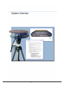
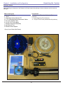
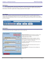
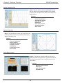
Desktop Antenna Measurement System
Model 6000
1
NOTICE
This Publication, including all photographs, illustrations and software is protected under international
copyright laws, with all rights reserved . Neither this manual, nor any of the material contained herein,
may be reproduced without the express written consent of Diamond Engineering. The information in
this document is subject to change without notice. Diamond Engineering makes no representations or
warranties of merchantability or fitness for any particular purpose. Further Diamond Engineering
reserves the right to revise this publication and to make changes from time to time in the content
hereof without obligation of Diamond Engineering to notify any person of such version changes.
Trademarks
IBM, VGA and PS/2 are registered trademarks of International Business Machines.
AMD is a registered trademark of Advanced Micro Devices Inc.
Intel, Pentium III/4 Are registered trademarks of Intel Corporation
Microsoft, and Windows NT/95/98/ME/2000/XP are registered trademarks of Microsoft Corporation.
VEE, VEE Runtime, and Agilent are registered trademarks of Agilent Corporation.
HP, HPIB, are registered trademarks of the Hewlett Packard Company.
Anritsu, Scorption are registered trademarks of the Anritsu Corporation.
Labview is a registered trademark of the National Instruments Corporation
Matlab is a registered trademark of Mathworks.
2
Table Of Contents
NOTICE .........................................................................................................................2
Introduction ............................................................................................................................................................ 6
System Overview ................................................................................................................................ 7
Key Features .......................................................................................................................................................... 7
Minimum System Requirements ....................................................................................................... 8
USB Port Platform Controller Unit .................................................................................................... 9
Parallel Port Platform Controller Unit .............................................................................................. 10
Chapter 1 - Installation and Configuration ..................................................................................... 12
Tripod and Elevation Unit Assembly .................................................................................................................. 13
Attaching the optional thrust plate- .................................................................................................................... 14
Attaching the cables ............................................................................................................................................ 15
Installing the Software ........................................................................................................................................ 16
Connecting the Controller and Installing the drivers. (Blue USB models Only) ............................................. 16
Installing the Parallel Port drivers (Pre-2005 Parallel interface units ONLY) .................................................. 17
Installing the Userport.Sys Driver (Required for Windows NT, 2000, And XP Professional users) ................ 17
VEE Runtime I/O Configuration .......................................................................................................................... 18
Calibrating/Setting the Vertical Movement to 0 Degrees -- See Also Vertical Calibration Settings ............ 20
Platform Positioning Test. ................................................................................................................................... 20
Special Installation Notes ................................................................................................................................... 21
Measurement Settings ......................................................................................................................................... 24
Instrument Selection and Settings ..................................................................................................................... 24
Chapter 2 - Software Overview ........................................................................................................ 24
Measurement Settings ......................................................................................................................................... 25
Receive Instrument -Spctrum Analyzer Settings .............................................................................................. 25
Measurement Settings ......................................................................................................................................... 26
Calibration Settings ............................................................................................................................................ 27
Measurement Controls ........................................................................................................................................ 28
Post Measurement Options ................................................................................................................................. 28
Meaurement Status and Displays ...................................................................................................................... 29
Data Processing Introduction .............................................................................................................................. 30
Data Registers ...................................................................................................................................................... 31
Visualization Options .......................................................................................................................................... 32
Measurement Calculator ..................................................................................................................................... 34
Dipole Link Simulator ......................................................................................................................................... 34
Vertical Swing Correction ................................................................................................................................... 34
Chapter 3 - Making Measurements ................................................................................................. 35
Performing a Scalar Calibration ........................................................................................................................ 36
Making a basic Horizontal/Azimuth Measurement ........................................................................................... 37
Making a basic Vertical/Elevation Measurement .............................................................................................. 37
Performing an AZ/EL Scan Measurement ......................................................................................................... 38
Chapter 4 - Using the Data Processing Feature ............................................................................ 40
Data Processing Screenshot ............................................................................................................................... 40
Saving and Loading Measurement Data Sets. .................................................................................................. 41
Viewing and working with measurements in 3D ............................................................................................. 42
Viewing and working with the Dynamic Amplitude Plot ................................................................................. 43
Using the Measurement Calculator / Register Math Function. ........................................................................ 45
Exporting Data ..................................................................................................................................................... 47
Using the Dipole and Isotropic Link Calculator- ................................................................................................ 49
Group Delay Function ......................................................................................................................................... 51
Chapter 5 - Troubleshooting and Service ...................................................................................... 54
Troubleshooting ................................................................................................................................................... 54
Warranty Information .......................................................................................................................................... 55
Replacement Parts .............................................................................................................................................. 55
Contact Information ............................................................................................................................................. 55
3
4
5
Introduction
Congratulations on your purchase of a Diamond Engineering
Desktop Antenna Measurement System! Also Known As DAMS
Diamond Engineering’s Desktop Antenna Measurement System has been designed to aid in
the testing and development of small to medium sized Antennas. Using state of the art software this
system enables you to make many different types of measurements with complete user-definable
configuration settings. The advanced Processing Feature enables you to not only plot 3D graphs of
the measurements, but save and recall those measurements for future use or comparison. Using the
Group Delay function will enable you to calculate the exact distance of the Test Antenna, Identify
Multipath rays, and eliminate the need to use another measuring device. Our software also allows you
to export your data to a 3rd party application or spreadsheet.
This manual will fully assist you step by step with Assembling, configuring, and using the
Desktop Antenna System. To achieve the full functionality of the rotator system we expect you to have
some prior knowledge about the concepts and theories about Microwaves and Antenna Design and
Development before using this software and rotator unit.
We cannot emphasize enough about the importance of fully reading and understanding this
manual before using this piece of equipment to avoid any risk of damaging the unit and possibly
voiding your warranty.
Best Regards, The Diamond Engineering Team
6
Features
System Overview
Key Features
·
Light Weight- Platform is made of high quality, light weight Acrylic material for easy portability
·
USB Port Connectivity- Unit easily connects to the computer using a standard USB cable.
·
User Friendly Software- Our software has been designed to be understood easily to ensure the
shortest time to successful Antenna Measurement.
·
Quality Components- The rotator unit is built only with the best of components for long lasting
reliability.
·
Compatibility- Our Software supports a wide range of network analyzers and instruments that
use the GPIB / 488.1/2 and SCPI methods of communication.
·
Phase/Angle Measurement-Software can measure All four Vector S-Parameters over a
specified frequency range at each measurement point.
·
2-axis movement- 360 Degrees Horizontal at 1/4 degrees per measurement to +/- 45 degrees
vertical movement angle at 1 degree per step.
·
DC to 18 Ghz. Measurement Range- A wide frequency use range allows for a more diversified
range of antennas that can be tested with the system.
·
Rotary SMA Joint- Using a custom developed “Near Zero” noise Rotary Joint the system can
make accurate measurements without jeopardizing signal integrity.
·
Data Processing Feature-Designed for post measurement processing you can perform a range of
functions such as:
o
o
o
o
o
o
o
o
o
o
o
o
Complete 3D Visualization for All Frequencies and Angles
3D Azimuth/Elevation plots for true 3D data representation.
Ability to save and Recall Data Sets from RAM or local Disk
Group Delay (distance calculation)
Spherical 3D plots
Ability to work with 4 different data sets at once
Ability to map over 50,000 Different measurement Points onto one 3D chart
Real-time Data over Movement V.S. Frequency
Dipole Link Calculator
Calculator for modifying measurement results and comparing antennas
Export your data to a Spreadsheet or 3rd part application such as MatLAB
Dipole Link Simulator allows creation of simulated dipole antennas
7
Requirements
System Overview
Minimum System Requirements
•
•
•
•
•
•
•
•
AMD/Pentium Class Computer with 1000 Mhz. Processor Or Higher (2 Ghz or Higher Recommended)
512 MB Ram
500 Megabytes Hard Disk Space
1 Available USB Port
1024x768 Display Resolution (Minimum)
Windows 95/98/ME/NT/2000/XP Operating Systems are supported
*Windows XP home is not compatible with the Parallel Port Model
Keyboard and Mouse
Compatible Network Analyzer or Power Meter/Spectrum Analyzer and Signal Generator.
As of the date of this maual the following Insturments are are currently supported by the Standard
DAMs Software.
VECTOR NETWORK ANALYZERS
-HP/Agilent 8510 Series
-HP/Agilent 8714 Series
-HP/Agilent 8720 Series
-HP/Agilent 8753 Series
-HP/Agilent 5071 Series
-Wiltron/Anritsu 46xx Series Analyzers (Scorpion)
-Rhode & Schwarz ZVx Series
SIGNAL GENERATORS
-HP 83650 Series
-HP 8350 Series
POWER METERS
-Elva DPM-10
-HP436A
-HP437B
-ML2438A (antritsu)
SPECTRUM ANALYERS
-HP8565 Series
•
Printer (optional) for printing Measured Antenna Plots
To Find System Information:
- Right Click on “my computer” on your
windows desktop and select Properties
8
USB Port Platform Controller Unit
System Overview
The USB Platform Control unit is a highly accurate Microprocessor based stepper controller. Movement signals are
sent from the measurment PC to the controller unit where precision stepping sequences are generated. We also offer a
development kit enabling you to write your own software to control the platform.
Platform Controller rear view
Platform Controller top view
9
Parallel Port Platform Controller Unit
System Overview
The Platform Control unit controls the positioning of the Horizontal and Vertical movements based on signals
recieved from the Computer’s Parallel Port. We also offer a Platfrom development kit which will allow you to adapt the
DAMS Platform to your own software using a special DLL library.
Control Unit Front View
Control Unit Side View
10
11
Unpacking the System
Chapter 1 - Installation and Configuration
Package Contents
Upon receiving your shipment of the Rotator Unit Please inspect the package to ensure all pieces are there and not
damaged
Accessories
10. Digital Level/Elevation Calibration Tool (optional)
11. Laser Alignment Tool (Optional)
12. Acrylic Thrust Plate (assembled with platform)
Main components
1. Positioner Platform
2. Tripod
3. Users Manual with Software CD
4. 2- 10’ Calibrated SMA measurement Cables
5. 20’ (6.2m) Parallel Cable
6. 12v AC to DC wall adapter
7. Elevation Movement Assembly
8. Hex Wrench Tool.
9. Elevation Mount Spacer
-Copy of your Order (Not Shown)
12
Tripod Assembly
Chapter 1 - Installation and Configuration
Tripod and Elevation Unit Assembly
The rotator unit has been shipped to you either complete in a matter that requires Minimal effort to assemble.
BEFORE YOU BEGIN: Unpack ALL items and ensure there is no damage or missing parts.
-Vertical Assembly
1. Unfold the Tripod and extend the top of the tripod 1/2 way and secure the height adjustment- (Fig. 1)
2. IMPORTANT! Take the grey vertical mount spacer and snap it onto the very top of the tripod
neck(fig. 2) Without this piece your unit will not make elevation measurements accuratly.
3. atttach the vertical assembly onto the top of the tripod using the included hex wrench so the top
edge of the vertical assembly is touching the bottom edge of the vertical spacer. (fig 3)
Fig 1- Extend the Tripod
Fig 2- Attach vertical Spacer
Fig 3- Attach vertical AssemblyEnsure the Vertical Actuator Rod
will have adequate clearance and
will not hit the tripod leg.
13
Platform Assembly
Chapter 1 - Installation and Configuration
Connecting the platform and vertical actuator.
1. Ensure that the Azimuth of the
tripod is unlocked.
2.Place the Tripod head in a
horizontal position and tighten the
locking screw (Loosen screw after
assembly)
4. Loosen the Tilt Lock (Pic 2) enough
to allow the platform to tilt and connect
the vertical actuator rod to the platform ,
tighten the locknut to ensure the rod
does not disconnect.
3. Align the colored piece of tape on the
platform with the tape on the tripod head
and insert the platform into the head at a
30 degree angle, the head will automatically lock the platform into position.
Attaching the optional thrust plate-
Applies to Acrylic and Aluminum models.
Attach the Thrust Plate using the 4 includeded
10-32x1/4” Screws. be sure not to overtighten screws
and if using your own screws be sure they do not hit
the metal bearing below.
14
Cable Connections
Chapter 1 - Installation and Configuration
Attaching the cables
You should have received 5 Seperate Cables and a power supply with your DAMS System.
1. 2- 10 Ft. Custom Calibrated SMA cable.(1-20’ Cable Optional)
2. 1- USB cable.
3. 2- 6m Platform control cables
Step 1. connect the USB cable to the Platform Controller. DO NOT CONNECT TO PC YET.
Step 2. connect the Power Supply wire to the Platform Controller.
Step 3. connect one end of the Calibrated SMA cable to the bottom of the platform.
Step 4. Attach other end of SMA cable to your Analyzer. **USE CARE** cable damage can compromise antenna
results.
Step 5. Connect the straight end of the yellow cable with the black band on the connector to the
“Horizontal” port on the Platform Controller and the non-banded cable to the “vertical” port.
Step 6. Connect the other ends the yellow cables to the platform. the banded right-angle connector connects to the
turntable. and the non-banded connector goes to the vertical actuator.
15
Software and Hardware Installation
Chapter 1 - Installation and Configuration
Installing the Software
1. Place Software CD in CD-ROM drive, The CD Menu should Start Automatically, If the menu does
not start automatically run setup.exe from your CD-ROM in “My Computer” or from Windows Explorer
2.Click next/ok through all Following Screens.
3. Before the software is finished installing , the Agilent Runtime setup will start, Continue through this
setup as you would a normal software installation.
4. After installation is complete the Software can be found on your desktop and in the start menu
under“DAMS”
Note To NT/200/XP Pro. Users! If you using a Parallel Port Controller— You must install the UserPort
driver discussed on the next page.
Connecting the Controller and Installing the drivers. (Blue USB models Only)
1. Connect the DAMS Platform Controller to the Computer using the included USB Cable. A window
should appear indicating that a new device has been found. Do not select the option to automatically
search for the latest driver!.
2. Click the Box labled Search Manually then click “Next”
3. Select CD-ROM
4, Click Next, You will then be prompted that the driver has not passed the WHQL certification. select the
“Continue Anyways” button.
5. Click Finish.
6. A new window will pop up indicating another device has been found, repeat steps 2-5 above.
7. You have now installed the DAMS Platform Controller and must continue with the Instrument Configu
ration.
16
Software Configuration
Chapter 1 - Installation and Configuration
Connecting the controller and installing the Parallel Port drivers (Pre-2005 Parallel interface units ONLY)
Installing the Userport.Sys Driver (Required for Windows NT, 2000, And XP Professional users)
NOTE: If you recieved a Pre-Configured Laptop From us, the Steps below have already been performed
-you will ony need to follow the steps below if you are Re-Installing the Operating System.
Overview
This guide will Assist you with the Required Changes that must me made to windows XP Professional before the software and platform will function correctly
Note about Windows XP: The Antenna Measurement Software Has only been tested and is only supported on the
Professional version of Microsoft Windows XP .
(LPT) Parallel Port Driver Installation Instructions:
Step 1:
The software installation has placed a Folder named “UserPort” located in the “C:\DAMS” Folder.
The userport.sys file allows the Windows XP operating system to communicate with the parallel port and control the
platform. Follow the instructions bellow to install the Userport.sys Driver.
1. Go to the “C:\dams\userport\” folder and copy the
“Userport.sys” file to the windows
system32\Drivers Folder. it is usually located in
“C:\windows\system32\drivers”
2. Run the Userport.Exe program as shown at right
and Select the I/O range you wish to use and
Press Start. (if you do not know which ports to leave
open just press start and the defaults will be used)
-- For additional Information Please read the
Userport.PDF located in the Userport Folder ---
Step 2:
Setting the Compatibility mode for VEE Runtime 6.0 (XP PRO ONLY!)
In order for the software to work absolutly correctly we reccomend setting
the Windows XP compatibility mode to Windows 98/Me Mode for less
chances of errors caused by the windows XP Kernel.
1. Open “My Computer” located in the Start Menu
2. Open your “C:” Drive
3. Double click on the “Program Files” Folder
4. Double Click “Agilent” then double click the “Vee Pro Runtime”
Folder.
17
Software Configuration
Chapter 1 - Installation and Configuration
VEE Runtime I/O Configuration
You must complete these steps for the Sofware
to communicate with your network analyzer!.
1. Click Start -> Programs->Agilent VEE pro 6.0
Runtime-> I/O Config
2. Turn on you Network Analyzer and Click the
“Find Instruments button.
3. You should see your network analyzer appear
in the list
The instrument number consists of the GPIB
controller ID number and the Instrument number
Example: ID (newinstrument@1416) 14=Nat inst
GPIB controller 16=Analyzer ID #
4. Select your analyzer from the list and Click on the “Properties
button” You should see the window to the right, Change the
name that is shown to one from the list below that matches your
analyzer.
Network Analyzer
HP 8510 series Analyzers
HP 8714 series Analyzers
HP 8720 series Analyzers
HP 8753 series Analyzers
HP 5071 series Analyzers
Anritsu Scorpion Analyzers
Rhode & Schwarz RS series
Signal Generator
HP 83650B Signal Gen.
HP 8350 Sweep Generator
“Name” setting
HP8510
HP8714
HP8720
HP8753
HP5071
Scorpion
RSZVR
“Name” setting
HP836
HP8350
Spectrum Analyzer
HP 8565 Series
“Name” setting
HP8565
Power Meter
HP 436A Power Meter
HP 437B Power Meter
Anritsu ML2438A
Anritsu ML4803A
ELVA-1 DPM 10
“Name” setting
HP436
HP437
ML2438
ML4803
DPM10
5. Press the “Advanced” button to bring up the Advanced Properties Dialog Box.
Set the Instrument Timeout to 15 seconds. Press OK , then OK, then “SAVE”. You have now
successfully completed the Analyzer Configuration Process.
18
Tripod Compatibility Information
The DAMS system has been designed so that it will operate with most any tripod, when purchasing a new tripod
you must ensure that all of the parts from the current system will fit onto the new trupod without angle or clearance
problems. Once you are ready to configure the software please read the “DAMS Application note / Tips and Tricks” for a
complete description and howto calibrate the vertical movement with a Tripod other than the one that was included with
your Antenna Measurement System. If you need Assistance you are welcome to call or e-mail us and we will be glad to
help.
19
System Test
Chapter 1 - Installation and Configuration
Calibrating/Setting the Vertical Movement to 0 Degrees -- See Also Vertical Calibration Settings
In order for the software to move the platform correctly on the vertical axis you must have the platform at 0 degrees when
starting the DAMS Softtware - or the platform must match the vertical position shown in the software before moving vertically.
If the Platform Angle and Software Angle do not match, Use the Jog buttons to move the platform to the level
position, you can change the Change jog distance by using the pulldown.
Platform Positioning Test.
1. Turn on the Platform Controller
2. Start the rotator software, Click Start -> Programs -> DAMS ->DAMS x.xx
3. Click the orange “Manual Move” button located in the upper left hand section of the software. The platform should
now horzontally move the number of times specified in the “Total Number of Measurements” window completing a
360 degree sweep.
4. Set the Vertical Differential slider to a value of -5 degrees and press the green “Manual Move” button, the platform
should now move to -5 degrees. Slide the slider back to 0 and press the “Manual Move” button. the platform
should now return to it’s starting position.
****If the Rotator Unit successfully performed the above functions, the rotator platform is fully functional and is ready
for Use.****
6. If The Rotator Unit does not Perform one or more of the above tests please refer to the Troubleshooting Section
located on Page 43
20
Installation Notes
Chapter 1 - Installation and Configuration
Special Installation Notes
SCREEN SLEEPERS and Power Saving options.
Be sure to disable screen sleepers, Power Saving Features and other
Applications, which may cause GPIB or dll to crash.
Other Running ApplicationsThe DAMs Software requires a large amount of CPU and System Resources. We advise you not to have any other
applications running while the DAMs Software is operating. Other Programs may cause the Platform to move
inaccurately.
Reporting BugsDuring some certain complicated/untested scenarios a failure may occur, If this happens, Please let us know. We will be
able to address the problem and offer a hot fix faster if the error is reported. Please send all errors and questions about
software operation to [email protected]
21
22
Chapter 2
23
Measurement Settings
Chapter 2 - Software Overview
Measurement Settings
Instrument Selection and Settings
You can now choose from multiple combinations of instruments such as a Signal Generator and Power Meter or Signal
Generator and Spectrum Analyzer.
Available Modes of Operation
1. VNA ONLY
2. Signal Generator and Power Meter
3. Signal Generator and Spectrum Analyzer
4. Signal Generator and Multimeter
5. Special Recieve Only Mode.
6. Emulation Mode. (Simulated Dipole Measurement)
(NOTE: Any instrument that you want to select must be
configured in the VEE I/O Configuration program prior to
selection)
Source Instrument Settings
NOTE: These settings also apply for the RECEIVE
ONLY instrument.
Start / Stop Frequency- Enter the frequency in GHz
Decimals are ok , example: 450Mhz = .45
Number of points- Similar to a VNA configuration
you may choose the number of frequency points for
the sweep, click the “Freq Increments” window to
display the calculated Frequency Step.
Output Power- Sets the output power of the Signal
Generator. format is dBm.
Receive Instrument -Power Meter Settings
Trigger Mode- Changes the way the power meter
reads the sensor, this setting is only applied to
certain meters.
Trigger Delay- This sets the delay / Settling time
between when the Signal generator is called and the
power meter is queried for a reading. format is in
seconds. Example: 1/10 second = .10
Sweep Delay- this sets the number of seconds the
signal generator will wait before initiating the sweep.
this allows larger antennas a chance to completely
stop moving.
24
Measurement Settings
Chapter 2 - Software Overview
Measurement Settings
Receive Instrument -Spctrum Analyzer Settings
Bandwidth- Sets the bandwidth window on the
spectrum analyzer , the smaller the window the faster
the sweep. Format is in GHz.
Resolution-Sets the Frequency Resolution of the
spectrum analyzer sweep. Inplut format is in MHz.
Trigger Mode- Changes the way the power meter
reads the sensor, this setting is only applied to
certain meters.
Trigger Delay- This sets the delay / Settling time
between when the Signal generator is called and the
power meter is queried for a reading. format is in
seconds. Example: 1/10 second = .10
Sweep Delay- this sets the number of seconds the
signal generator will wait before initiating the sweep.
this allows larger antennas a chance to completely
stop moving.
25
Measurement Settings
Chapter 2 - Software Overview
Measurement Settings
Azimuth setup
Degrees Per Measurement- Displays the CURRENT
degrees-per measurement based off of total degrees sliderand
the degrees per measurement settings (note: This window
may indicate a different value than the pulldown, remember
this is the current setting)
Number of measurements readout- Dislplays the
CURRENT total number of measurements that will be made
based on the settings below.
Total Rotation Slider- This slider sets the total number of
degrees the Platform will sweep the antenna (360 default)
Degrees Per Measurement Pulldown- This drop down list
contains all of the possible degrees per measurement
combinations for the selected total rotation.
Direction- Click this button to change the rotation direction of
the platform
Manual Move- When this button is pressed the platform will
simulate the movement sequence without actually measuring
data.
Elevation setup
Vertical Slider- Use this slider to set the vertical angle that
you would like the platform to move to.
Vertical Step size- This sets the vertical measurement and
movement resolution, the default setting is 5 degrees per
measurement but you can go as low as 1 degree if you wish.
Limit Check- You have the option of having the software
monitor the movement of the platoform to advise you if your
selected vertical movement will cause the platform to
exceed the vertical limits.
Manual Move- When this button is pressed the platform will
simulate the movement sequence without actually measuring
data.
Platform Settings and Calibration
Platform Speed- Use this slider to set speed at which the
platform will rotate, 1 being slowest and 90 being fatest
Motor Settings- Contains configuration settings relating to
motor type, gear ratio and motor driver. Please see section 12 for more details.
Vertical Calibration- This button opens the vertical
calibration window described in section 1-2 of the manual -
26
Calibration Settings
Chapter 2 - Software Overview
Calibration Settings
Scalar Calibration
This feature anables you to make a scalar calibration using your Signal Generator and Recieve source. An in depth
explinaton and example is located in chapter 3 - Calibrating your system.
Averaging- in cases of large ammounts
of background noise you may want to
average the calibration measurements.
Save Cal- Save your callibration to a file
on your computer.
Load Cal - Load a calibration file from
your computer.
Pad (dB)- if using a post amp with
attenuator , you need to enter the attenuator value in this window.
Power Head Cal- This button invokes the
power sensor cal menu.
(NOTE: If using a powe meter with NonProgrammed sensor You MUST load or
enter a Power Sensor cal table before
performing a scalar calibration)
Power Sensor Calibration
The Power Head / Sensor calibration menu is located in the Scalar Calibration section.
Enter PM cal factors- you can enter the
calibration table directly to check
compatibiliy
Compile Array- Compile the manually
entered Cal factors and display them on
the chart below
Load Cal - Load a calibration file from
your computer.
Load from Notepad File- Load a file
containing a Cal-Factor lookup table.
Sample notepad file- This file shows
you how your Cal-Factor notepad file
needs to look
Test- Enter a frequency within the value of
the cal factor table and you will see the
corresponding exact Cal-Factor in the
“Calculated CF” window.
27
Measurement Controls
Chapter 2 - Sofware Overview
Measurement Controls
Measure Horiz. Sweep- When this button is pressed, the software will begin making measurements by moving the
platform horizontally , then retrieving the data from the network analyzer. The button will remain “greyed out” while the
antenna measurement is in progress
Measure Vert. Sweep- When this button is pressed, the software will begin making measurements by moving the
platform horizontally , then retrieving the data from the network analyzer. The button will remain “greyed out” while the
antenna measurement is in progress
Scan VH- When this button is pressed, the software will begin what is caled a scan sweep, the software will make a
complete horizontal measurement then move to the next vertical position and make another complete horizontal sweep.
this process will continue until the platform reaches the ending vertical position.
Reset Accumulator- When this button is pressed, the software will begin making measurements by moving the platform
horizontally , then retrieving the data from the network analyzer. The button will remain “greyed out” while the antenna
measurement is in progress
Post Measurement Options
Move to Max Signal - When this button is pressed, the software will analyze the measurements you have jsut
made to find the position where the antenna had the maximum gain , the software will then move the antenna to
the maximum signal position.
Proceed to Data Processing- Once you have completed making your measurements and you click this button you
will be taken to a section of the software that will allow you to view/manipulate any prt of the measurement. The Data
Processing section also allows you to view the data in many different formats including , Polar, Mag, and 3D
Export Reg 0 - When you have completed a measurement you can instantly export the data set to an outside file
for the ability to import the data into a speadsheet or use in a 3rd party plotting or processing program.
28
Measurement Status and Displays
Chapter 2 - Software Overview
Meaurement Status and Displays
Measurement Status window
The measurement status window displays all of the current Measurement parameters and will update automatically
During the measurement process.
Graphical Status Displays
The Graphical status windows allow you to view the Real-Time data as it is captured from the Network Analyzer. All Status
Graphs display the center measurement frequency.
Center Frequency Amplitude Plot- This plot displays the Amplitude in dB of the measured Antenna.
Antenna Polar Radiation Patern- This plot displays the Real-Time pattern of the measured Antenna
High Res Plot - Display a high resolution MatLab Polar plot of your measured Antenna at the Center Frequency.
Rotation Tracker- This plot shows the current position of the platform, the Horizontal Axis is shown with circular data
points, and the Vertical movement is shown with data points on the center plane of the plot.
Clear Plot- Each plot has it’s own “Clear-Plot’ button , this will clear all current data from the plot
29
Data Processing
Chapter 2 - Software Overview
Data Processing Introduction
The Data Processing Feature is your gateway to unlocking the data contained within your antenna measurements. After making your initial measurement of the Antenna you can press the “Data Procesing” button located in the
“Post Measurement Options” window of the main software page and you will be taken to the screen shown below.
This section of the manual will describe all of the functions located in the Data Processing feature.
30
Data Processing
Chapter 2 - Software Overview
Data Registers
When working with data in the Data Processing feature all of the data is stored in registers, these regesters alow
you to have “Holding Space” for partictular data sets. this is very useful for working with multiple measurements from
other antennas. There are 5 registers total, 4 storage registers and 1 Active register.
Active Register
Once you have completed a measurement and open the Data Processing Feature, The entire data set from your
measurement will automatically be placed into the “Active” Data register. The Active register is applied to all functions
including 3D plots and Data Export functions. with the exception of the Measurement Calculator which can pull data from
any of the 5 registers.
Data Registers
The Data Storage Registers offer space to put up to 4 different measurement sets that you can recall at any point in time,
you can also save the entire set of 4 registers to disc for use at a later time.
Data Storage Button- When this button is pressed , all of
the data in the Active Register is stored to whichever
storage button that you chose.
Recall Button- When this button is pushed , all of the
data in the chosen storage register will be written to the
active register for viewing or modification.
Load Reg 1-4 From Disc- This button will load a set of 4
registers from the disc.
Save Reg 1-4 To Disc- This button will save a set of 4
registers to the disc.
Clear All Registers- This button will clear all data from
registers 1-4.
31
Data Processing
Chapter 2 - Software Overview
Visualization Options
The data visualuzation options enables you to view the Antenna Data in a wide variety of formats.
Azmuth vs. Frequency vs. Amplitide 3D Plot
About: This plot is the most versatile of the 3D plots and
will gve you a good idea of the frequency response Vs.
Rotation of the Antenna you have measured . If you have
made Az/El measurements you can use the Az/El 3D plot
for a more detailed view.
Features
View entire data set at once
Full Plot Rotation
Zoom In/Out feature
Line and Notation Tools
Exportable to common graphic formats
Printable
Azimuth vs. Elevation vs. Amplitude 3D Plot
About: After you make a Az/El measurement you can
view the Azimuth vs. Elevation for any measured
frequency using the Az/El 3D Plot use the Azimuth Vs
Frequency 3D plot to view frequency response to aid in
the selection of of the single frequency.
Features
View Az/El Data for any Frequency point
Full Plot Rotation
Zoom In/Out feature
Line and Notation Tools
Exportable to common graphic formats
Printable
32
Data Processing
Chapter 2 - Software Overview
Dynamic Amplitude Plot
About: This plot offers a Linear or Log Mag 2D look into
the Gain Pattern of the measured Antenna for a specified
frequency point. This plot is also useful in examining Az/El
Measurements
Features
Linear or Log Format
Automatically updates
Keep Max Function
Data Export
Auto Scale Function
Selectable Markers
Zoom In/Out
Dynamic Polar Plot
About: This plot offers a Linear or Log Polar 2D look into
the Rotation Gain Pattern of the measured Antenna for a
specified frequency point.
Features
Linear or Log Format
Scale Functions
Automatically updates
Keep Max Function
Data Export
Auto Scale Function
Zoom In/Out
Group Delay Function
About: This features allows the analysis of the Group
Delay and Path Propogation Data. you can also make an
accurate measurement of the antenna distances using
this feature.
Features
Distance Scale Functions
Data Export
Auto Scale Function
Printable Plots
33
Data Processing
Chapter 2 - Software Overview
Measurement Calculator
Use this option to perform arithmetic operations on the measurement registers. For example if you make measurements on one antenna and wish to compare the results to another antenna at each point of rotation and each frequency. Or if you have a calibrated reference antenna an wish to normalize additional measurements to the max or min
value of the reference antenna. Remember all measurement data is linear so you may want to “LOG” the data before
doing math. If you select MAX or MIN then all measurement elements will be replaced with MAX or MIN. This creates a
normalization reference if you do your math correctly.
Dipole Link Simulator
The Diple Link Simulator is used to create ideal dipole
measurements based on a set of physical and environmental
factors. These calculated measurements can be imported directly to
the measurement calculator for comparison with Measured Data.
Vertical Swing Correction
The Vertical Swing Correction
tool is used to compensate for the tilt
of the platform when making Vertical /
Elevation Measurements.
34
35
System Calibration
Chapter 3 - Making Measurements
Important---- If you are using a VNA this information does not apply to you.
Performing a Scalar Calibration
1. Be sure Platform Power supply is securely attached and plugged in
3. Turn Platform Power ON.
4.
Selet the Source Instrument you plan to use, After selection click the “Settings” button located below the icon.
5. Click the “Cal System button
6. Connect the power meter to the top of the DAMs System.
7, Press the left “Begin Calibration” button, Follow on screen directions.
36
Basic Measurements
Chapter 3 - Making Measurements
Making a basic Horizontal/Azimuth Measurement
1. Be sure Platform Power supply is securely attached and plugged in
2. Attach antenna to rotator platform with SMA connector
3. Turn Platform Power ON.
4. On your analyzer select S21, POLAR Plot and the proper Calibration set Example: 4 to 6 Ghz @ 201 Points.
*if your analyzer has not been calibrated, you need to follow the calibration procedure listed in chapter 1
5.
Select the total Number of degrees you want the platform to move using the “Total Degrees Slider”, the total
amount will be shown in the slider window.
6. Select the “Degrees Per Measurement” setting of your choice using the associated Slider. The “Total number
of measurements” window will be updated once a selection has been made.
7. Select your Direction using the CW/CCW selection
8. Press the “Measure Horiz Sweep” Button to start the measurement Process
9. During the measurement process you will see the Rotator Platform moving and center frequency data starting to
appear on your screen. The “Measure Horiz Sweep” button will remain greyed out for the duration of the
measurements. Once the button has returned to its normal state you may enter the “Advanced Processing” section
or perform other Post Measurement options.
Making a basic Vertical/Elevation Measurement
1. Be sure Platform controller is turned on and connected.
2. Attach antenna to rotator platform with SMA connector
3. Start the DAMS Software.
4. On your analyzer select S21, POLAR Plot and the proper Calibration set Example: 4 to 6 Ghz @ 201 Points.
5. Be sure the platform angle matches the position displayed on the screen, if it is not correct refer to the vertical
calibration information located on page -6. Set the vertical position slider to the desired start position and press the Manual Move button, this will move the
platform to the beginning Elevation position.
7. Select the desired stop position on the vertical slider.
8. Press the “Measure Vert Sweep” Button to start the measurement Process
9. During the measurement process you will see the Rotator Platform moving and center frequency data starting to
appear on your screen. The “Measure Vert Sweep” button will remain greyed out for the duration of the
measurements. Once the button has returned to its normal state you may enter the “Advanced Processing”
section or perform other Post Measurement options.
37
Az/El Scan Measurements
Chapter 3 - Making Measurements
Performing an AZ/EL Scan Measurement
1. Be sure Rotator Power is Securely attached and plugged in
2. Attach Antenna to rotator platform using a SMA connector
3. Turn Platform Power ON.
4. On your analyzer select S21, POLAR Plot and the proper instrument
state -Example: 4 to 6 Ghz @ 201 Points.
5.
The Total Degrees Slider must be set to 360 degrees or the software
will not sort measurements correctly.
6. Select the total Number of degrees you want the platform to move using the “Total Degrees Slider”, the total
amount will be shown in the slider window.
*remember the number of measurements you select is multiplied by the number of elevation measurement points,
this will cause large files and may cause problems for some computers depending on resolution)
7. Select your Direction using the “CW/CCW” selection
8. Move the platform to the Elevation start position using the vertical slider and the “Manual Move” button.
(If the vertical position of the platform does not match the software readout - level the platform first, Pg. --)
9. Set the Vertical movement slider to the desited elevation stop position.
10. Press the “Scan AZ/EL” button to begin making measurements.
11. During the measurement process you will see the Rotator Platform make a complete horizontal sweep then
move to the next desired elevation point and will repeat the horinzontal sweep. You should also see some data
starting to appear on your screen, The Scan AZ/EL button will remain greyed out during the measurement process.
Once the button returns to it’s normal state your measuring process is complete and you may continue on to Data
Processing.
38
39
Chapter 4 - Using the Data Processing Feature
Data Processing Screenshot
Introduction
Use the Data Proceessing section to work with the data you collected after you make any Antenna
Measurements. This feature allows complete control over the data including the ability to completely manipulate the data
using a large set of math operators as well as compare the current antenna to another Antenna or a calibrated refernece
antenna. A complete set of plotting options allow you visualize your data in a multitude of formats. This section of the
manual will assist you with getting the most out of your Antenna Measurement System. If you are not familliar with any of
the terms mentioned in this chapter , please refer to the Software Overview located on page.
40
Chapter 4 - Using the Data Processing Feature
Data Processing Feature
Saving and Loading Measurement Data Sets.
All Measurement Data is stored in Data Sets, each Data Set consists of a group of 4 Data Registers. These 4
Registers are used only for storing and recalling data within the Data Processing feature, the Data Sets can be recalled
or saved to disc at any point in time. There is one register called the “Active Register”, Any plots, graphs, and export
features will be based off of this register, but this register is considered “temporary” and will not be saved to disc, any
Active Register data that you want to save must be placed into one of the 4 Data Registers.
Once you enter the Data Processing section after making an Antenna Measurement, all of the measurement
data will be placed in the “Active Register” . To save this data you would click the button labled “Data Storage Reg 1” this
will place all of the active register data into Data Storage Register 1 and cause a red * to be places next to that data
register. To save this data set to the hard drive you would press the “Save Reg 1-4 to disc” button.
Data Storage Button- When this button is pressed , all of
the data in the Active Register is stored to whichever
storage button that you chose.
Recall Button- When this button is pushed , all of the
data in the chosen storage register will be written to the
active register for viewing or modification.
Load Reg 1-4 From Disc- This button will load a set of 4
registers from the disc.
Save Reg 1-4 To Disc- This button will save a set of 4
registers to the disc.
Clear All Registers- This button will clear all data from
registers 1-4.
Quick Tip : After entering Data Processing Immediatly press the “Data Storage Reg 1” button to keep the original
measurement data available
41
Chapter 4 - Using the Data Processing Feature
Data Processing Feature
Viewing and working with measurements in 3D
Press any of the 3D Buttons to View the “Active Register” Data in 3D Using the MatLab Viewing Interface.
Viewing 3D Azimuth Measurements
1. Be Sure there is data in the “Active Register, if there is no data
you must recall data from one of the storage registers or make a
Measurement.
2. Press the “View 3D Az Plot” button.
3. Depending on the size of your measurement and the speed of
your computer it may take up to 2 minutes for your 3D plot to
appear on the screen.
Viewing 3D Az/El Measurements
1. Be Sure there is data in the “Active Register, if there is no data
you must recall data from one of the storage registers or make a
Measurement.
2. You can only view 1 frequecy at a time using the Az/El 3D
Plots, when you press the “View 3D Az/El” measurements you
will be prompted to choose a frequency to view.
3. Depending on the size of your measurement and the speed of
your computer it may take up to 2 minutes for your 3D plot to
appear on the screen.
QUICK TIP: Use the Amplitude plot to get a reference of the
frequency response of the antenna.
Working With 3D Data
Below are a few common functions that you can do with the 3D plots.
To Rotate a Plot- Click Tools -> Rotate 3D
To Print a Plot- Click File->Print
To Label a Plot- Click Tools -> Add -> Text
To save a Plot- Click File -> Save (Saved File compatible with matlab viewer only)
To Export as BMP Image File- Click File -> Export
42
Chapter 4 - Using the Data Processing Feature
Data Processing Feature
Viewing and working with the Dynamic Amplitude Plot
Follow the Instructions below to view your data using the Dynamic Amplitude Plot located in the Data Processing
feature of the software. Remember, The Dynamic Amplitude Plot will only plot the data that is contained in the Active
Register.
Instructions:
1. From the Main Data Processing Page click on Amplitude Frequency Plot and you will be taken to
the screen shown below
2. Select Log or Linear Data View.
3. Click “Auto Scale” to view all of the data
4. Slide the Frequency Slider to the desired frequency.
5. To Eliminate Flickering , Click the “Freeze” Button located on the left side of the plot.
6. Click the Export Data button to export the data for the specific frequency to a file with a user
defined format.
7.To Save a copy of the plot image you must use the Windows Screen Capture feature by pressing
the “Print Screen” button on your keyboard and pasting the copied image into Photoshop or other
QUICK TIP: Right-Click the plot to see a list of visualization options such as zoom, and scaling functions.
Dynamic Amplitude Plot Screenshot
43
Chapter 4 - Using the Data Processing Feature
Data Processing Feature
Viewing and working with the Polar Plot display
Follow the Instructions below to view your data using the Polar Plot located in the Data Processing feature of the
software. Remember, The Polar Plot will only plot the data that is contained in the Active Register.
Instructions:
1. From the Main Data Processing Page click on “Polar Plot” and you will be taken to the screen
shown below
2. Select Log or Linear Data View.
3. Click “Auto Scale” to view all of the data
4. Slide the Frequency Slider to the desired frequency. (The plot will automatically update).
5. To Eliminate Flickering , Click the “Freeze” Button located on the left side of the plot. (NOTE: The
plot will not automatically update while the “Freeze” button is pressed”
6. Click the Export Data button if you want to export the data for the specific frequency to a file with
a user defined format.
7. You can change the dB/Div using the selction box in the lower left nad corner of the Plot window.
8. To Save a copy of the plot image you must use the Windows Screen Capture feature by pressing
the “Print Screen” button on your keyboard and pasting the copied image into Photoshop or other
image editing program.
QUICK TIP: Right-Click the plot to see a list of visualization options such as zoom, and scaling functions.
Polar Plot Screenshot
44
Chapter 4 - Using the Data Processing Feature
Data Processing Feature
Using the Measurement Calculator / Register Math Function.
Use this option to perform arithmetic operations on the measurement registers. For example if you make
measurements on one antenna and wish to compare the results to another antenna at each point of rotation and each
frequency. Or if you have a calibrated reference antenna an wish to normalize additional measurements to the max or
min value of the reference antenna. Remember all measurement data is linear so you may want to “LOG” the data
before doing math. If you select MAX or MIN then all measurement elements will be replaced with MAX or MIN. This
creates a normalization reference if you do your math correctly.
Register Math / Calculator Screenshot
Understanding the Register Math Functions
Measurement data is initially stored in the Active registerwhen you leave the main software page and enter the
advanced processing section. When you proceed to the Data Processing Feature you have a choice of 4 additional
registers in which to store Reg0.
The measurement format is:
dataReg0-4[Mag,Phase,(Hpos,Vpos),0/1,freq]
Each time you press the Reg calculator = sign the results are save to the Active Register. You can then save those
results to any one of the 4 original Regs. Be sure to have saved the original to disc as it will be over written.
Math Functions
Linear : When highlighted the Reg# to the right is to be used as S21 in vector format Arithmetic is performed using
vector components
LinearMag : When highlighted the Magnitude of Reg # to the right is to be Logged (dB) and used as a scalar array in
all arithmetic operations. The angle information is remains in the original Reg# but is lost in the calculator.
LOGmag: When highlighted the Reg# to the right is to be used as
10LOG(S21^2) in scalar format The
frequency S21 angle information remains in the original Reg # but is lost in the calculator.
^2 :
When highlighted the Reg# to the right is to be used in complex format and squared
SQRT : When highlighted the Reg# to the right is to be used complex format ^(1/2)
Max : When highlighted the Reg# to the right Maximum Linear value is to be used in all matrix arithmetic. This
provides a good way to normalize measurements. The frequency S21 angle information remains in the original Reg#
but is lost in the calculator.
Min :
When highlighted the Reg# to the right Minimum Linear value is to be used in all matrix arithmetic. This
provides a good way to normalize measurements. The frequency S21 angle information remains in the original Reg#
but is lost in the calculator.
Constant :> Use the constant option to +-/* a constant to the first register set (left) This is useful when you wish to
add level shifts such as 3dB for HV polarization measurements not accounted for anywhere else.
45
Chapter 4 - Using the Data Processing Feature
Using the Measurement Calculator / Register Math Function.
Data Processing Feature
Contd.
Clip Function
Use this to create a threshold level. A ZERO value clip causes software to ignore clipping and resume normal calculator
mode.
For example lets say the you wish to not include data points smaller than some low level value such as <-50dBM.
Enter the value -50 into the constant window aUnderstanding the Register Math Functions nd highlight “Clip”. This
will operate on only the data from the first set (left of the +-*/). Any magnitude values LESS that the clip value will be set
EQUAL to the clip value.
Notice: the plotting functions will be affected by the clip value. Use this to scale and expand the plots. Notice also that
the calculator can be used to change the plot scales from linear to log or to add offset to measurements.
TERM 1 MULTIPLIER
LINEAR
linMag
LogMag
Works with
+,+,-,*,/
+,-,*,/
TERM 2 MULTIPLIER All functions above plus Constant
IMPORTANT: Not all combinations of Math are possible. Be sure you
have the same size data array
46
Chapter 4 - Using the Data Processing Feature
Data Processing Feature
Exporting Data
Measurement Export Process
Most simulators make use of space delimiter data files. Space delimited data files were originally established for SParameter measurements and are still the standard today. A space delimited file is easily copied and paste into a
spreadsheet, word processor or text editor. Microwave Office
and Agilent both use the original “Touchstone” format established by Compact Engineering in the 70’s. This program is
a universal data exporter.
It may be used for any properly formatted program variable or disc measurement file.
Use the switches to select which columns of data you would like in your file.
Text File Format
Scalar| Complex |Complex |Complex |Complex
(Space Delimited)
Column 1 “Scalar” is a 1D array with real
elements
Columns 2 to 5 are 1D arrays with complex
elements
The colors associate function with switches
Or:
NumM Adata Bdata
NumM is the number of measurements in array
format.
VARIABLES: - All variables are single column arrays
Scalar = The first real array toggled by switch 2 to be written to disc A real array used to establish the number of rows
for all switches for export
NumM = A real array which contains the number of measurements. Begins at 1 and ends at the number of
measurements in steps of 1. Normally you would set Scalar by typing Nnum in the scalar window below the scalar
switch.
Adata = Linear power and rotation angle = (P , @ Ang) A column array in complex form Ang = Any and all movement
Horiz or Vertical.
LogAdata = 10*Log(|Adata|) For dB. Does not affect angle.
47
Chapter 4 - Using the Data Processing Feature
Data Processing Feature
Measurement Export Process
Contd.
Adata is your measurement data array in complex format from the baisc page 1 software
The first column is a scalar array and can set the count for example “frequencies” or angle. You can do this in one of two
ways. Enter a known one dimensional array variable such as “NumM”. The program variable “NumM” is a 1-D array
otherwise only a single row will be written. The number of elements in the NumM array will set column 1 variable
“Scalar” (number of data ROWS). Column1 “Scalar” array is automatically set
from the variable you enter into the window unless you press one of the other two Set Scalar buttons.
Make your own Scalar array. Enter the Start, Stop, NumPts such as
Frequencys in the windows below the Scalar switch. Remember if switch is in the up position Scalar will still be used for
the number of rows but not written to the output file.
Notice there is also a SET SCALAR button below column 2. You may choose to set the number of rows using the size of
column 2.
This will set Scalar and if Scalar is present in column 1 window and switch 1 isin the down position then the output file
will include the row count or whatever.
Any one of the switches in the up position will skip that parameter in the output file. Note that for basic Antenna rotation
measurements the frequency is constant while the path loss and angle is the program measurement complex variable
“Adata”. I you wanted to create a text
based output file for a spreadsheet which contains the results of a rotation and measurement set then set all switches
tothe up position except for switch 2 (or 3 or 4 or 5). Then enter Adata into window 2 below switch 2. Press the Set
Scalar button in column 2. Then export the data. The resulting text file will contain two columns. Column 1 = Magnitude
and column 2 will contain the position. Open the file with Note Pad and use copy & paste to transfer into spreadsheet. If
you wanted column 1 to contain the row count then use Set Scalar in column 1. Enter the number of measurements
(n)from page 1 software (in the slider window) and a start stop(n) number. Then export. stop number (1
Notice that there are “From Variable” “From Disc” check boxes below each Complex switch. When From Variable is
checked the data is retrieved from the variable in the box below the switch at the time of export.
When From Disc is checked you are prompted for a disc data file name at the time of export. The disc file format is that
used by VeePRO complex measurement format ie. (Mag, @Ang) in a single column. This proves
invaluable for a wide variety of vector measurements from VNA’s.
48
Chapter 4 - Using the Data Processing Feature
Data Processing Feature
Using the Dipole and Isotropic Link CalculatorUse the ideal dipole to simulate an entire link measurement set. Then you may perform calculator operations that you
can use to normalize and compare your measurements to.
The calculations are for any dipole length over any frequency range for any rotation sequence. Be advised the
calculation can become enormous if you
choose a very long or very short lengths compared to a wavelength. The Si and Ci sin(x)/x and cos(x)/x intergrals are
numerically calculated.
It is important to understand how the link works. The
dipole current is sinusoidal. The current is assumed the
same over all frequencies.
The radiated power at all frequencies is the same. If
Imax is to be constant over the frequency band then the
total radiated power changes with RadR. Maintaining
Imax with frequency requires an imaginary tuner
between the dipole and the VNA... Once you have
calculated the Tx dipole gain you must complete the link
by defining the receive aperture. If you save the dipole
gain to a REG and perform a a plot function you may
see that the dipole gain peaks at frequencies other than
the 1/4 wave frequency. This is because you must
multiply the dipole gain by the apertures at distance.
Think of the aperture as the hole through which the
dipole radiated power is received. The effective hole
area is inversely proportional to frequency or 1/f^2 in
power.
After each calculation return to the advanced menu and store the results into Re1 and Reg2. Note that these results are
linear power.
If you are planning to compare your link measurements to this ideal dipole link
then you need to set the frequency and rotation start,stop&step to the same values.
Set the PTx(dBM)to your VNA power + DAMs loss. Make sure the number of VNA measurement points are the
same. This matches the data matrix dimensions and extents with your actual measurements.
The dipole will simulate an entire measurement set, performing rotation and measurements at each point. It is
assumed the dipole has been matched (S11=0) at each measurement.
You should try a few calculations to get a feel for the CPU time involved before actually making
measurements. Once the calculations are complete the calculate button reappears. You may exit the
process at any time if you get tired of waiting. The plot of radiation resistance appears first. After which the
pattern calculations progress much faster. This results in one gain(f,Angle).
Note the results are linear not dB. From this point you will want to store these results in a REG.
Then you must decide how to define the Rx antenna and use the calculator to calculate the classical link
equation.
Calculate the Rx Aperture. Use this to calculate and fill
the frequency array with the area aperture equation for use with the receive antenna.
49
Chapter 4 - Using the Data Processing Feature
Using the Dipole and Isotropic Link Calculator
Data Processing Feature
Contd.
Once you have saved your dipole array into REG1 (or 2,3,4) calculate the Aperture array and save the results
into REG2. Now use the calculator to multiply REG1 x REG2. The result is the entire link gain normalized to
the Rx antenna gain.
Save the results into a REG3. Now choose a receive antenna. You could go back into the dipole section and
calculate another dipole for Rx.
Save these results into REG4. Multiply REG4 X REG3. This gives the entire path gain over Tx rotation and
frequency.
********—THE Rx Aperture— If the Rx antenna is isotropic (GRx=1) then the “Calculate Rx Aperture” is
the receive power for two isotropic radiators (one Tx and one Rx) at distance R. It is as the figure
above except that each dipole is replaced with an ideal infinitesimal isotropic antenna where the Tx
radiator is fed with the PTx power (converted to linear)
********—ABOUT PHASE— The phase angle for the dipole is in absolute degrees. This makes it easy to
calculate group delay
50
Chapter 4 - Using the Data Processing Feature
Data Processing Feature
Group Delay Function
Group delay is the derivative (slope) of the transmission phase angle. For passive circuit elements the group
delay is linear and may be calculated from two measurements. It is important that the ratio of the frequency deltawavelength is less that the physical distance between the measurement. If this is not the case then either the frequency
Resolution must be increased or the delay will need to be integer scaled. The scale integer is INT(d/wavelength).
Wavelength is that wavelength associated with the difference frequency (or step frequency). Periodic spikes will occur in
the group delay plot. Non-periodic spikes represent the Multipath or some other source of distortion.
Be advised this software does not perform vector corrections for free space measurements. The corrected group delay
is applied only toThe display. Use the EXPORT button on the display to save the display values to disc. Note that if you
made measurements and saved them to the disc or into a Reg that they will NOT be corrected for system delay but
WILL be corrected for system loss. You Should note this in your file Document item to avoid incorrect displays or resave. To correct the group delay (locally) check the radial “Correct for system delay” (left). The plots will automatically
update allowing you see both the corrected and uncorrected profiles.
Group Delay Screenshot
51
52
53
Chapter 5 - Troubleshooting and Service
Troubleshooting Operation
Troubleshooting
Problem- Red Light does not come on
Possible Causes- Power Supply is not connected correctly, Power Switch is not in the ON position
Solution- Check all of the Items listed above and if everything is OK and light still does not come on please contact us
immediately for service.
Problem- Red Light comes on but rotator does not move
Possible Causes- Parallel cable is not connected to the LPT1. Port on the computer, the port is not configured properly
or disabled on the computer.
Solution-Check all connections and verify that the parallel port on the computer is properly configured for LPT1.
Problem- Green Lights on controller are on and the horizontal moves but the vertical does nothing.
Possible causes- Vertical Movement cable is not properly connected between movement assembly and the rotator
platform. Bad software installation
Solution- Disconnect and re connect movement cable to verify correct insertion. Re install rotator software.
Problem- Running WinNT,2000,XP Pro it comes up with a red window indicating that a serious error has occurred.
Possible Causes- Userport.sys is not installed
Solution- Install Or Re-Install the UserPort.sys Driver
Problem- Analyzer does not initialize on Program start/Program Crashes with ID error
Possible Causes- Analyzer ID is set incorrectly, Missing Instrument Driver, GPIB Card/Bus is not working correctly
Solution- Using Vee-Runtime I/O manager verify the ID number is set correctly. And run the GPIB Pre-Test to verify
Connectivity.
**If you are experiencing any of the above problems and cannot determine the cause, please contact us as soon as
possible so we can address the problem and send you replacement parts as soon as we can.
54
Chapter 5 - Troubleshooting and Service
Service and Contact Info.
Warranty Information
The Antenna Measurement System is guaranteed for 2 years on parts and labor from the time it was received by you. If
there is a problem with the product please send us a picture or write a very detailed description of the problem, If we
determine that you have a faulty unit or bad part we will ship you a replacement part or unit with a self addressed box to
send the defective unit back with
Replacement Parts
If you ever need a replacement part for your rotator unit, Please call us or e-mail us for faster response and pricing
information. Most Repairs are covered under warranty except for damages resulting from obvious abuse or misuse of the
product
Contact Information
Visit us on the Web at Http://www.DiamondEng.net
Main Headquarters
Diamond Engineering
P.O. Box 2037
Diamond Springs, CA 95619
Phone- (530)626-3857
Fax- (530)626-0495
Technical Support and Warranty
Name- James Martin
Email- [email protected]
Administrative and financial questions
Name- Mike Hillbun
Email- [email protected]
55