Download ensim hydrologic - Civil and Environmental Engineering

Title Page
Copyright Information
Copyright ©1998-2006 Canadian Hydraulics Centre, National Research Council
EnSim Hydrologic was developed with Microsoft© Visual C++, Copyright ©1994-1998, Microsoft Corporation. All rights
Reserved.
MFC. Microsoft Corporation. Copyright ©1997. All Rights Reserved.
OpenGL. Silicon Graphics, Inc. Copyright ©1993. All Rights Reserved.
EnSim Hydrologic is protected by HASP Software Protection System, Copyright © Aladdin Knowledge Systems, 1985-2002.
All Rights Reserved.
WATFLOOD/SPL9, Copyright © by N. Kouwen, 1986-2000
Supported Foreign Files:
TOPAZ, Grazinglands Research Laboratory and Department of Geography, University of Saskatchewan.
ArcInfo® Grid, Environmental Systems Research Institute, Inc. Copyright ©1997-2002.
ArcView® Shape Files, Environmental Systems Research Institute, Inc. Copyright ©1997-2002.
DTED® or CDED® DEM, National Imagery and Mapping Angency (NIMA).
MapInfo® Interchange Format, MapInfo Corporation. Copyright ©2002.
Surfer® Grid, Golden Software, Inc. Copyright ©1994-1997.
GeoTIFF Library, Copyright ©1995, Niles D. Ritter. Copyright ©1999, Frank Warmerdam.
TIFF Library, Copyright ©1988-1997, Sam Leffler. Copyright ©1991-1997, Silicon Graphics, Inc.
iii
ACKNOWLEDGEMENTS
EnSim Hydrologic has been a collaborative effort funded in part by:
• Environment Canada, Ottawa, Ontario
Special thanks are directed at several individuals who have supported the EnSim Hydrologic
project by serving as beta testers and providing technical feedback, constructive criticism, and
helpful comments:
• Raymond Bourdages, Technical Development, Water Survey Branch, Environment
Canada, Ottawa, Ontario
• Stuart Hamilton, Pacific Yukon Region, Meteorological Service of Canada, Environment
Canada, Vancouver, British Columbia
• David Hutchinson, Pacific Yukon Region, Meteorological Service of Canada, Environment
Canada, Vancouver, British Columbia
• Nicholas Kouwen, Department of Civil Engineering, University of Waterloo, Waterloo,
Ontario
• David Morin, Environmental Protection Services, Environment Canada, Gatineau, Quebec
• Champa Neale, Water Survey Canada, Environment Canada, Ottawa, Ontario
• Al Pietroniro, National Hydrology Research Centre, Environment Canada, Saskatoon,
Saskatchewan
• Maurice Sydor, Data Integration Modelling and Analysis, Environment Canada, Gatineau,
Quebec
• Jean-Guy Zakrevsky, Water Survey Canada, Environment Canada, Ottawa, Ontario
Thanks are also given to the many users who have provided feedback and suggestions for other
applications within the EnSim family.
v
Table of Contents
1
ENSIM CORE . . . . . . . . . . . . . . . . . . . . . . . . . . . . . . . . . . . . . 1
1.1 A QUICK OVERVIEW . . . . . . . . . . . . . . . . . . . . . . . . . . . . . . . . . . . . . . .
1.1.1 The EnSim Simulation Environment . . . . . . . . . . . . . . . . . . . . . . .
1.1.2 Getting Started . . . . . . . . . . . . . . . . . . . . . . . . . . . . . . . . . . . . . . .
1.1.3 Getting Help with EnSim . . . . . . . . . . . . . . . . . . . . . . . . . . . . . . . .
1.1.3.1
1
1
1
2
Conventions in EnSim Help . . . . . . . . . . . . . . . . . . . . . . . . . . . . . . . 2
1.2 THE WORKSPACE . . . . . . . . . . . . . . . . . . . . . . . . . . . . . . . . . . . . . . . . . 3
1.2.1 Managing Objects in the WorkSpace . . . . . . . . . . . . . . . . . . . . . . 3
1.2.2 Saving and Loading The WorkSpace . . . . . . . . . . . . . . . . . . . . . . 6
• To Save a WorkSpace: . . . . . . . . . . . . . . . . . . . . . . . . . . . . . . . . . . . . . . . 6
• To Load a WorkSpace: . . . . . . . . . . . . . . . . . . . . . . . . . . . . . . . . . . . . . . . 6
1.3 THE ENSIM INTERFACE . . . . . . . . . . . . . . . . . . . . . . . . . . . . . . . . . . . . . 7
1.3.1 The Menu Bar . . . . . . . . . . . . . . . . . . . . . . . . . . . . . . . . . . . . . . . . 7
1.3.2 The Tool Bar . . . . . . . . . . . . . . . . . . . . . . . . . . . . . . . . . . . . . . . . . 8
1.3.3 Shortcut Menus . . . . . . . . . . . . . . . . . . . . . . . . . . . . . . . . . . . . . . . 8
1.4 DATA ITEMS . . . . . . . . . . . . . . . . . . . . . . . . . . . . . . . . . . . . . . . . . . . . . 9
1.4.1 Loading and Importing Data Items . . . . . . . . . . . . . . . . . . . . . . . 10
1.4.1.1
1.4.1.2
1.4.2
1.4.3
Native Data Items . . . . . . . . . . . . . . . . . . . . . . . . . . . . . . . . . . . . . . 10
Foreign Data Items . . . . . . . . . . . . . . . . . . . . . . . . . . . . . . . . . . . . . 11
Saving and Exporting Data Items . . . . . . . . . . . . . . . . . . . . . . . . 11
Properties of Data Items . . . . . . . . . . . . . . . . . . . . . . . . . . . . . . . 16
1.4.3.1 Display Properties . . . . . . . . . . . . . . . . . . . . . . . . . . . . . . . . . . . . .
1.4.3.1.1 Rendering Options . . . . . . . . . . . . . . . . . . . . . . . . . . . . . . . . . .
1.4.3.1.2 Vertical Display Options . . . . . . . . . . . . . . . . . . . . . . . . . . . . . .
1.4.3.1.3 Other Display Options . . . . . . . . . . . . . . . . . . . . . . . . . . . . . . . .
1.4.3.2 Colour Scale . . . . . . . . . . . . . . . . . . . . . . . . . . . . . . . . . . . . . . . . . .
17
17
18
19
19
• To edit the colour scale: . . . . . . . . . . . . . . . . . . . . . . . . . . . . . . . . . . . . . . 20
• To apply a previously created colour scale: . . . . . . . . . . . . . . . . . . . . . . . 20
1.4.3.3 Data Attributes . . . . . . . . . . . . . . . . . . . . . . . . . . . . . . . . . . . . . . . .
1.4.3.4 Spatial . . . . . . . . . . . . . . . . . . . . . . . . . . . . . . . . . . . . . . . . . . . . . .
1.4.3.4.1 Attributes . . . . . . . . . . . . . . . . . . . . . . . . . . . . . . . . . . . . . . . . . .
1.4.3.4.2 Coordinate Systems . . . . . . . . . . . . . . . . . . . . . . . . . . . . . . . . .
1.4.3.4.3 Coordinate System - Converting Projections . . . . . . . . . . . . . .
20
24
25
25
26
• To change the projection of the object: . . . . . . . . . . . . . . . . . . . . . . . . . . 26
1.4.3.4.4 Coordinate Systems - Assigning Projections . . . . . . . . . . . . . . 26
• To assign a coordinate system to an object: . . . . . . . . . . . . . . . . . . . . . . 26
1.4.3.4.5 Ellipsoids . . . . . . . . . . . . . . . . . . . . . . . . . . . . . . . . . . . . . . . . . .
1.4.3.4.6 Selecting a Coordinate System . . . . . . . . . . . . . . . . . . . . . . . .
1.4.3.5 Meta Data . . . . . . . . . . . . . . . . . . . . . . . . . . . . . . . . . . . . . . . . . . . .
1.4.3.6 Applying Changes to an Object’s Properties . . . . . . . . . . . . . . . . .
27
28
30
30
vii
EnSim Hydrologic
1.4.3.7
September 2007
Copying Data Item Properties . . . . . . . . . . . . . . . . . . . . . . . . . . . . 30
• To copy data item properties: . . . . . . . . . . . . . . . . . . . . . . . . . . . . . . . . . 30
1.5 VIEWS . . . . . . . . . . . . . . . . . . . . . . . . . . . . . . . . . . . . . . . . . . . . . . . . . .32
1.5.1 Creating a View Window . . . . . . . . . . . . . . . . . . . . . . . . . . . . . . .32
1.5.2 Removing a View Window . . . . . . . . . . . . . . . . . . . . . . . . . . . . . .32
1.5.3 Properties Shared by all View Types . . . . . . . . . . . . . . . . . . . . . .32
1.5.3.1
1.5.4
The 1D View Window . . . . . . . . . . . . . . . . . . . . . . . . . . . . . . . . . .33
1.5.4.1
1.5.4.2
1.5.4.3
1.5.4.4
1.5.5
Labels of Axes in a 1D View . . . . . . . . . . . . . . . . . . . . . . . . . . . . .
The 1D View Window Status Bar . . . . . . . . . . . . . . . . . . . . . . . . . .
Manipulating the 1D View . . . . . . . . . . . . . . . . . . . . . . . . . . . . . . .
Display Properties of the 1D View Window . . . . . . . . . . . . . . . . . .
34
34
35
35
The Polar View Window . . . . . . . . . . . . . . . . . . . . . . . . . . . . . . . .36
1.5.5.1
1.5.5.2
1.5.5.3
1.5.5.4
1.5.6
The Properties Dialog . . . . . . . . . . . . . . . . . . . . . . . . . . . . . . . . . . 33
Coordinates in a Polar View . . . . . . . . . . . . . . . . . . . . . . . . . . . . . .
The Polar View Window Status Bar . . . . . . . . . . . . . . . . . . . . . . . .
Manipulating the Polar View . . . . . . . . . . . . . . . . . . . . . . . . . . . . . .
Display Properties of the Polar View Window . . . . . . . . . . . . . . . .
37
37
37
38
The 2D View Window . . . . . . . . . . . . . . . . . . . . . . . . . . . . . . . . . .39
1.5.6.1
1.5.6.2
1.5.6.3
Coordinate Systems and Units in 2D Views . . . . . . . . . . . . . . . . . . 39
The 2D Window Status Bar . . . . . . . . . . . . . . . . . . . . . . . . . . . . . . 40
Manipulating the 2D View . . . . . . . . . . . . . . . . . . . . . . . . . . . . . . . 40
1.5.6.4
Display Properties of the 2D Window . . . . . . . . . . . . . . . . . . . . . . . 41
• To move a data item already in the view to the top layer: . . . . . . . . . . . 40
1.5.7
The 3D View Window . . . . . . . . . . . . . . . . . . . . . . . . . . . . . . . . . .42
1.5.7.1
1.5.7.2
1.5.7.3
1.5.8
The Spherical View Window . . . . . . . . . . . . . . . . . . . . . . . . . . . . .46
1.5.8.1
1.5.8.2
1.5.8.3
1.5.9
The 3D Window Status Bar . . . . . . . . . . . . . . . . . . . . . . . . . . . . . . 43
Manipulating the 3D View . . . . . . . . . . . . . . . . . . . . . . . . . . . . . . . 43
Display Properties of the 3D View Window . . . . . . . . . . . . . . . . . . 45
The Spherical View Window Status Bar . . . . . . . . . . . . . . . . . . . . . 46
Manipulating the Spherical View . . . . . . . . . . . . . . . . . . . . . . . . . . 47
Display Properties of the Spherical View Window . . . . . . . . . . . . . 47
The Report View Window . . . . . . . . . . . . . . . . . . . . . . . . . . . . . . .49
1.5.9.1
1.5.9.2
1.5.9.3
The Report View Window Status Bar . . . . . . . . . . . . . . . . . . . . . . . 49
The Report View Window Tool Bar . . . . . . . . . . . . . . . . . . . . . . . . 50
Manipulating the Report View . . . . . . . . . . . . . . . . . . . . . . . . . . . . 51
• To add a view to a report: . . . . . . . . . . . . . . . . . . . . . . . . . . . . . . . . . . . .
• To manipulate a view that has been added to a report: . . . . . . . . . . . . .
• To change the order of objects in the report: . . . . . . . . . . . . . . . . . . . . .
• To change the border around an object in the report: . . . . . . . . . . . . . .
1.5.9.4
1.5.9.5
51
51
51
51
Report View Window Page Setup Properties . . . . . . . . . . . . . . . . . 52
Report View Templates . . . . . . . . . . . . . . . . . . . . . . . . . . . . . . . . . 53
• To create a report template: . . . . . . . . . . . . . . . . . . . . . . . . . . . . . . . . . . 53
• To use a report template: . . . . . . . . . . . . . . . . . . . . . . . . . . . . . . . . . . . . 53
1.5.10 View Decorations . . . . . . . . . . . . . . . . . . . . . . . . . . . . . . . . . . . . .53
1.5.10.1 Legends . . . . . . . . . . . . . . . . . . . . . . . . . . . . . . . . . . . . . . . . . . . . . 54
1.5.10.1.1Colour Scale Legends . . . . . . . . . . . . . . . . . . . . . . . . . . . . . . . 54
viii
Table of Contents
September 2007
1.5.10.1.2Independent Legends . . . . . . . . . . . . . . . . . . . . . . . . . . . . . . . . 56
• To create an independent legend: . . . . . . . . . . . . . . . . . . . . . . . . . . . . . . 56
• To edit an independent legend: . . . . . . . . . . . . . . . . . . . . . . . . . . . . . . . . 56
• The quick legend: . . . . . . . . . . . . . . . . . . . . . . . . . . . . . . . . . . . . . . . . . . .57
1.5.10.2 The Compass . . . . . . . . . . . . . . . . . . . . . . . . . . . . . . . . . . . . . . . . . 58
1.5.10.3 The Simulation Clock . . . . . . . . . . . . . . . . . . . . . . . . . . . . . . . . . . . 58
1.5.10.4 Labels . . . . . . . . . . . . . . . . . . . . . . . . . . . . . . . . . . . . . . . . . . . . . . . 59
• To create a label: . . . . . . . . . . . . . . . . . . . . . . . . . . . . . . . . . . . . . . . . . . .59
• To edit a label: . . . . . . . . . . . . . . . . . . . . . . . . . . . . . . . . . . . . . . . . . . . . . 60
1.5.11 Animation . . . . . . . . . . . . . . . . . . . . . . . . . . . . . . . . . . . . . . . . . . 60
1.5.12 Flight Paths . . . . . . . . . . . . . . . . . . . . . . . . . . . . . . . . . . . . . . . . . 61
• To create a new flight path: . . . . . . . . . . . . . . . . . . . . . . . . . . . . . . . . . . . 61
1.5.12.1 Flight Path Properties . . . . . . . . . . . . . . . . . . . . . . . . . . . . . . . . . . . 62
1.5.13 Synchronizing Two Views . . . . . . . . . . . . . . . . . . . . . . . . . . . . . . 62
• To synchronize Views: . . . . . . . . . . . . . . . . . . . . . . . . . . . . . . . . . . . . . . . 63
1.5.14 Saving and Copying Images . . . . . . . . . . . . . . . . . . . . . . . . . . . . 64
1.5.14.1 Recording . . . . . . . . . . . . . . . . . . . . . . . . . . . . . . . . . . . . . . . . . . . . 64
• To create a movie: . . . . . . . . . . . . . . . . . . . . . . . . . . . . . . . . . . . . . . . . . . 64
1.5.14.2 Copying to the Clipboard . . . . . . . . . . . . . . . . . . . . . . . . . . . . . . . . 66
• To copy the image of a view window to the clipboard: . . . . . . . . . . . . . . . 66
1.5.14.3 Printing . . . . . . . . . . . . . . . . . . . . . . . . . . . . . . . . . . . . . . . . . . . . . . 66
1.5.15 Troubleshooting in Views . . . . . . . . . . . . . . . . . . . . . . . . . . . . . . 66
1.6 TOOLS . . . . . . . . . . . . . . . . . . . . . . . . . . . . . . . . . . . . . . . . . . . . . . . . . 67
1.6.1 Creating New Data Items . . . . . . . . . . . . . . . . . . . . . . . . . . . . . . 67
1.6.1.1
Drawing Points . . . . . . . . . . . . . . . . . . . . . . . . . . . . . . . . . . . . . . . . 67
1.6.1.2
Drawing Lines and Closed Polylines . . . . . . . . . . . . . . . . . . . . . . . 68
• To create a point set: . . . . . . . . . . . . . . . . . . . . . . . . . . . . . . . . . . . . . . . . 67
• To create a line or polyline: . . . . . . . . . . . . . . . . . . . . . . . . . . . . . . . . . . . 68
• To create a closed line or polygon: . . . . . . . . . . . . . . . . . . . . . . . . . . . . . 68
1.6.1.3
1.6.1.4
1.6.1.5
1.6.2
Editing Data Items . . . . . . . . . . . . . . . . . . . . . . . . . . . . . . . . . . . . 71
1.6.2.1
1.6.2.2
1.6.2.3
1.6.2.4
1.6.3
1.6.4
Creating a New Regular Grid . . . . . . . . . . . . . . . . . . . . . . . . . . . . . 68
Creating a New Triangular Mesh . . . . . . . . . . . . . . . . . . . . . . . . . . 70
Creating a New Table Object . . . . . . . . . . . . . . . . . . . . . . . . . . . . . 71
Editing Attributes . . . . . . . . . . . . . . . . . . . . . . . . . . . . . . . . . . . . . .
Editing Points . . . . . . . . . . . . . . . . . . . . . . . . . . . . . . . . . . . . . . . . .
Editing Time Series . . . . . . . . . . . . . . . . . . . . . . . . . . . . . . . . . . . .
Resampling Lines and LineSets . . . . . . . . . . . . . . . . . . . . . . . . . . .
72
73
73
76
Resampling Time Series . . . . . . . . . . . . . . . . . . . . . . . . . . . . . . . 78
Probing Data . . . . . . . . . . . . . . . . . . . . . . . . . . . . . . . . . . . . . . . . 80
1.6.4.1
Data Probes . . . . . . . . . . . . . . . . . . . . . . . . . . . . . . . . . . . . . . . . . . 80
• To probe data: . . . . . . . . . . . . . . . . . . . . . . . . . . . . . . . . . . . . . . . . . . . . . 80
1.6.4.2 The Live Cursor . . . . . . . . . . . . . . . . . . . . . . . . . . . . . . . . . . . . . . . 82
1.6.4.2.1 The Live Stream Lines Cursor . . . . . . . . . . . . . . . . . . . . . . . . . 83
• To save stream lines: . . . . . . . . . . . . . . . . . . . . . . . . . . . . . . . . . . . . . . . . 84
1.6.4.3
1.6.5
The Ruler . . . . . . . . . . . . . . . . . . . . . . . . . . . . . . . . . . . . . . . . . . . . 84
Extracting Data . . . . . . . . . . . . . . . . . . . . . . . . . . . . . . . . . . . . . . 85
ix
EnSim Hydrologic
September 2007
1.6.5.1 Extracting Surfaces . . . . . . . . . . . . . . . . . . . . . . . . . . . . . . . . . . . . 86
1.6.5.1.1 Extracting Temporal Statistics . . . . . . . . . . . . . . . . . . . . . . . . . 86
• To extract temporal statistics as a surface: . . . . . . . . . . . . . . . . . . . . . . 86
1.6.5.1.2 Extracting Slopes . . . . . . . . . . . . . . . . . . . . . . . . . . . . . . . . . . .
1.6.5.1.3 Extracting Aspects . . . . . . . . . . . . . . . . . . . . . . . . . . . . . . . . . .
1.6.5.1.4 Extracting Curvatures . . . . . . . . . . . . . . . . . . . . . . . . . . . . . . . .
1.6.5.2 Extracting Residuals . . . . . . . . . . . . . . . . . . . . . . . . . . . . . . . . . . .
1.6.5.3 Extracting Isolines . . . . . . . . . . . . . . . . . . . . . . . . . . . . . . . . . . . . .
87
88
89
90
91
• To extract an isoline: . . . . . . . . . . . . . . . . . . . . . . . . . . . . . . . . . . . . . . . . 91
1.6.5.4
Extracting Paths . . . . . . . . . . . . . . . . . . . . . . . . . . . . . . . . . . . . . . . 91
1.6.5.5
Extracting Points . . . . . . . . . . . . . . . . . . . . . . . . . . . . . . . . . . . . . . 91
• To extract a path: . . . . . . . . . . . . . . . . . . . . . . . . . . . . . . . . . . . . . . . . . . 91
• To extract points from a data item: . . . . . . . . . . . . . . . . . . . . . . . . . . . . . 92
1.6.5.6
Extracting Time Series . . . . . . . . . . . . . . . . . . . . . . . . . . . . . . . . . . 92
1.6.5.7
Extracting a Velocity Rose . . . . . . . . . . . . . . . . . . . . . . . . . . . . . . . 94
• To extract a time series: . . . . . . . . . . . . . . . . . . . . . . . . . . . . . . . . . . . . . 92
• To extract a velocity rose: . . . . . . . . . . . . . . . . . . . . . . . . . . . . . . . . . . . . 94
1.6.6
Create Vector Field . . . . . . . . . . . . . . . . . . . . . . . . . . . . . . . . . . . .96
• To create a vector grid or mesh: . . . . . . . . . . . . . . . . . . . . . . . . . . . . . . . 96
1.6.7
Computing a Distribution . . . . . . . . . . . . . . . . . . . . . . . . . . . . . . .97
• To create a distribution: . . . . . . . . . . . . . . . . . . . . . . . . . . . . . . . . . . . . . 97
1.6.8
Mapping Objects . . . . . . . . . . . . . . . . . . . . . . . . . . . . . . . . . . . . . .98
• To map objects: . . . . . . . . . . . . . . . . . . . . . . . . . . . . . . . . . . . . . . . . . . . 99
1.6.9
Calculators . . . . . . . . . . . . . . . . . . . . . . . . . . . . . . . . . . . . . . . . .100
1.6.9.1
The Calculator for Data Items . . . . . . . . . . . . . . . . . . . . . . . . . . . 100
1.6.9.2
The Calculator for Gridded Objects . . . . . . . . . . . . . . . . . . . . . . . 100
• To use the calculator: . . . . . . . . . . . . . . . . . . . . . . . . . . . . . . . . . . . . . . 100
• To use the calculator: . . . . . . . . . . . . . . . . . . . . . . . . . . . . . . . . . . . . . . 101
1.6.9.3
The Calculator for Time Series Objects . . . . . . . . . . . . . . . . . . . . 102
1.6.9.4
The Calculator Expressions . . . . . . . . . . . . . . . . . . . . . . . . . . . . . 104
• To use the calculator: . . . . . . . . . . . . . . . . . . . . . . . . . . . . . . . . . . . . . . 102
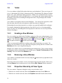
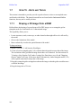
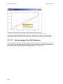
1.7 HOW TO - HINTS AND TRICKS . . . . . . . . . . . . . . . . . . . . . . . . . . . . . . .106
1.7.1 Draping a 3D Image Onto a DEM . . . . . . . . . . . . . . . . . . . . . . . .106
• To drape an image: . . . . . . . . . . . . . . . . . . . . . . . . . . . . . . . . . . . . . . . . 106
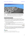
1.7.2
Extracting Cross-Sections from Gridded Data . . . . . . . . . . . . . .107
• To create a cross-section or 3D polyline: . . . . . . . . . . . . . . . . . . . . . . . 107
1.7.3
Extracting Cross-Sections from Points and Line Data . . . . . . . .108
• To create a cross-section or 3D polyline from points or line data: . . . . 108
1.7.4
Displaying Two Features of an Object Simultaneously . . . . . . .108
• Some other things to remember: . . . . . . . . . . . . . . . . . . . . . . . . . . . . . 109
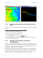
1.7.5
1.7.6
1.7.7
Displaying Isoline-Outlined Filled Contours . . . . . . . . . . . . . . . .109
Creating a Sloping Structure in a Rectangular Grid . . . . . . . . . .110
Extracting a Spatial Subset From a Larger Grid . . . . . . . . . . . . .111
• To define a spatial subset from a rectangular grid: . . . . . . . . . . . . . . . . 111
1.7.8
Extracting a Temporal Subset of Time-Varying Gridded Data . .111
• To extract a temporal subset: . . . . . . . . . . . . . . . . . . . . . . . . . . . . . . . . 112
1.7.9
x
Digitizing from an Imported Image . . . . . . . . . . . . . . . . . . . . . . .112
Table of Contents
September 2007
• To digitize from an imported image: . . . . . . . . . . . . . . . . . . . . . . . . . . . . 112
1.7.10 Georeferencing a non-georeferenced GeoTIFF . . . . . . . . . . . . 113
• To georeference a non-georeferenced tiff: . . . . . . . . . . . . . . . . . . . . . . . 113
1.7.11 Classification of a GeoTIFF Image . . . . . . . . . . . . . . . . . . . . . . 114
• To classify a GeoTIFF image: . . . . . . . . . . . . . . . . . . . . . . . . . . . . . . . . 114
• To create a Custom Theme: . . . . . . . . . . . . . . . . . . . . . . . . . . . . . . . . . 115
• To choose from a predefined theme: . . . . . . . . . . . . . . . . . . . . . . . . . . . 115
2
ENSIM HYDROLOGIC . . . . . . . . . . . . . . . . . . . . . . . . . . . . 117
2.1 WATERSHED OBJECTS . . . . . . . . . . . . . . . . . . . . . . . . . . . . . . . . . . . .
2.1.1 Opening an Existing Watershed Object . . . . . . . . . . . . . . . . . .
2.1.2 Importing a Watershed from Topaz . . . . . . . . . . . . . . . . . . . . . .
2.1.3 Creating a New Watershed Object . . . . . . . . . . . . . . . . . . . . . .
2.1.3.1
117
118
118
118
Watersheds . . . . . . . . . . . . . . . . . . . . . . . . . . . . . . . . . . . . . . . . . 119
• To delineate a watershed: . . . . . . . . . . . . . . . . . . . . . . . . . . . . . . . . . . . 120
2.1.3.2 DEMs . . . . . . . . . . . . . . . . . . . . . . . . . . . . . . . . . . . . . . . . . . . . . .
2.1.3.2.1 Checking for Errors and Editing the DEM . . . . . . . . . . . . . . . .
2.1.3.3 Channels and Flow Paths . . . . . . . . . . . . . . . . . . . . . . . . . . . . . .
2.1.3.3.1 Channel Attributes . . . . . . . . . . . . . . . . . . . . . . . . . . . . . . . . .
2.1.3.3.2 Displaying Channels . . . . . . . . . . . . . . . . . . . . . . . . . . . . . . . .
121
121
121
122
123
• To view more or fewer channels: . . . . . . . . . . . . . . . . . . . . . . . . . . . . . . 124
2.1.3.3.3 Editing the Channels . . . . . . . . . . . . . . . . . . . . . . . . . . . . . . . . 125
2.1.3.3.4 Using Predefined Channels . . . . . . . . . . . . . . . . . . . . . . . . . . 125
• To add a predefined channel to a Watershed: . . . . . . . . . . . . . . . . . . . . 127
2.1.3.3.5 Watershed or Basin Outlet Nodes . . . . . . . . . . . . . . . . . . . . . 127
• To select an outlet node: . . . . . . . . . . . . . . . . . . . . . . . . . . . . . . . . . . . . 128
• To select a channel node near a watershed outlet node: . . . . . . . . . . . 128
2.1.3.4 Basin or Watershed Boundaries . . . . . . . . . . . . . . . . . . . . . . . . . . 129
2.1.3.4.1 Creating and Removing Basins . . . . . . . . . . . . . . . . . . . . . . . 130
• To add a basin: . . . . . . . . . . . . . . . . . . . . . . . . . . . . . . . . . . . . . . . . . . . 130
• To remove a basin: . . . . . . . . . . . . . . . . . . . . . . . . . . . . . . . . . . . . . . . . 130
2.2 HYDROLOGIC TOOLS . . . . . . . . . . . . . . . . . . . . . . . . . . . . . . . . . . . . . 131
2.2.1 Watershed Tools . . . . . . . . . . . . . . . . . . . . . . . . . . . . . . . . . . . . 131
2.2.1.1
2.2.1.2
2.2.1.3
2.2.1.4
2.2.1.5
2.2.1.6
2.2.1.7
2.2.1.8
2.2.1.9
2.2.1.10
2.2.1.11
2.2.1.12
2.2.1.13
2.2.1.14
Extracting Drainage Directions . . . . . . . . . . . . . . . . . . . . . . . . . . .
Extracting Drainage Area . . . . . . . . . . . . . . . . . . . . . . . . . . . . . . .
Extracting Depression Fill . . . . . . . . . . . . . . . . . . . . . . . . . . . . . . .
Extracting Average Upslope Elevation . . . . . . . . . . . . . . . . . . . . .
Extracting Average Upslope Slope . . . . . . . . . . . . . . . . . . . . . . . .
Extracting Wetness Index . . . . . . . . . . . . . . . . . . . . . . . . . . . . . . .
Extracting Stream Power . . . . . . . . . . . . . . . . . . . . . . . . . . . . . . .
Extracting Relief Potential . . . . . . . . . . . . . . . . . . . . . . . . . . . . . .
Extracting Upstream Network . . . . . . . . . . . . . . . . . . . . . . . . . . . .
Extracting Downstream Reach . . . . . . . . . . . . . . . . . . . . . . . . . . .
Extracting Basin Network . . . . . . . . . . . . . . . . . . . . . . . . . . . . . . .
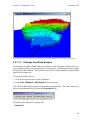
Extracting a Hypsographic Curve . . . . . . . . . . . . . . . . . . . . . . . . .
Extracting Basin Flow Path Distances . . . . . . . . . . . . . . . . . . . . .
Drainage Area Ratio Analysis . . . . . . . . . . . . . . . . . . . . . . . . . . .
131
132
133
134
135
135
136
137
137
138
139
139
140
141
xi
EnSim Hydrologic
September 2007
2.2.1.14.1Known Flow . . . . . . . . . . . . . . . . . . . . . . . . . . . . . . . . . . . . . . 142
2.2.1.14.2Computed Flow . . . . . . . . . . . . . . . . . . . . . . . . . . . . . . . . . . . 143
• To add a computed flow station: . . . . . . . . . . . . . . . . . . . . . . . . . . . . . . 143
2.2.1.15 Slope Analysis . . . . . . . . . . . . . . . . . . . . . . . . . . . . . . . . . . . . . . . 144
2.2.2
Rating Curve Analysis (RCA) . . . . . . . . . . . . . . . . . . . . . . . . . . .145
2.2.2.1 Background and Theory . . . . . . . . . . . . . . . . . . . . . . . . . . . . . . . .
2.2.2.1.1 Power Curve Fit . . . . . . . . . . . . . . . . . . . . . . . . . . . . . . . . . . .
2.2.2.1.2 Polynomial Curve Fit . . . . . . . . . . . . . . . . . . . . . . . . . . . . . . .
2.2.2.2 The Rating Curve Analysis Interface . . . . . . . . . . . . . . . . . . . . . .
145
145
146
146
• To perform an RCA on a HYDAT station: . . . . . . . . . . . . . . . . . . . . . . . 146
• To create an RCA from any two time series: . . . . . . . . . . . . . . . . . . . . 146
2.2.2.2.1 Working With Rating Curves . . . . . . . . . . . . . . . . . . . . . . . . . 149
• To adjust the rating curve by creating a subset: . . . . . . . . . . . . . . . . . . 149
• To inactivate an individual data point: . . . . . . . . . . . . . . . . . . . . . . . . . . 149
• To adjust the rating curve directly: . . . . . . . . . . . . . . . . . . . . . . . . . . . . 150
2.2.2.3
Opening an Existing RCA . . . . . . . . . . . . . . . . . . . . . . . . . . . . . . 154
• To open an RCA: . . . . . . . . . . . . . . . . . . . . . . . . . . . . . . . . . . . . . . . . . 154
2.2.2.4
Saving an RCA . . . . . . . . . . . . . . . . . . . . . . . . . . . . . . . . . . . . . . . 154
• To save an RCA: . . . . . . . . . . . . . . . . . . . . . . . . . . . . . . . . . . . . . . . . . 154
2.3 WATFLOOD . . . . . . . . . . . . . . . . . . . . . . . . . . . . . . . . . . . . . . . . . . .155
2.3.1 WATFLOOD Map Files . . . . . . . . . . . . . . . . . . . . . . . . . . . . . . . .155
2.3.1.1
2.3.1.2
Opening an Existing Watflood Map File . . . . . . . . . . . . . . . . . . . . 155
Creating a New Watflood Map File . . . . . . . . . . . . . . . . . . . . . . . 155
• To set map file specifications manually: . . . . . . . . . . . . . . . . . . . . . . . . 155
• To set map file specifications automatically: . . . . . . . . . . . . . . . . . . . . . 156
• To return to the default grid: . . . . . . . . . . . . . . . . . . . . . . . . . . . . . . . . . 157
2.3.1.3 Modelling Multiple Watersheds . . . . . . . . . . . . . . . . . . . . . . . . . . 158
2.3.1.4 Watflood Map Data Attributes . . . . . . . . . . . . . . . . . . . . . . . . . . . 159
2.3.1.4.1 Description of Data Attributes . . . . . . . . . . . . . . . . . . . . . . . . . 159
2.3.1.4.2 Calculating Default Data Attributes from the Watershed Object162
2.3.1.4.3 Displaying Different Data Attributes in the Watflood Map . . . . 162
• To display the same data attributes for all cells: . . . . . . . . . . . . . . . . . . 162
• To display all the data attributes for a single cell: . . . . . . . . . . . . . . . . . 163
2.3.1.5 Editing Watflood Map Data Attributes . . . . . . . . . . . . . . . . . . . . . 163
2.3.1.5.1 Adding Land Use Data Using Closed Polygons . . . . . . . . . . . 163
• To add land class data: . . . . . . . . . . . . . . . . . . . . . . . . . . . . . . . . . . . . . 164
• To map land use data: . . . . . . . . . . . . . . . . . . . . . . . . . . . . . . . . . . . . . 164
• Points to remember when applying land use data to a Watflood Map: . 166
2.3.1.5.2 Adding Land Use Data Using GeoTIFFs . . . . . . . . . . . . . . . . 166
• To map land use data: . . . . . . . . . . . . . . . . . . . . . . . . . . . . . . . . . . . . . 166
2.3.1.5.3 Editing Land Use Data . . . . . . . . . . . . . . . . . . . . . . . . . . . . . . 166
2.3.1.5.4 Resetting a Land Use Class . . . . . . . . . . . . . . . . . . . . . . . . . . 167
• To reset a land use class: . . . . . . . . . . . . . . . . . . . . . . . . . . . . . . . . . . . 167
2.3.1.6
2.3.2
Saving the Watflood Map . . . . . . . . . . . . . . . . . . . . . . . . . . . . . . . 167
Importing WATFLOOD Files . . . . . . . . . . . . . . . . . . . . . . . . . . . .167
2.3.2.1
Watflood Event File Properties . . . . . . . . . . . . . . . . . . . . . . . . . . . 168
• To save changes to the Event file: . . . . . . . . . . . . . . . . . . . . . . . . . . . . 168
2.3.3
2.3.4
xii
WATFLOOD Output . . . . . . . . . . . . . . . . . . . . . . . . . . . . . . . . . .169
Bankfull Animation . . . . . . . . . . . . . . . . . . . . . . . . . . . . . . . . . . .169
Table of Contents
September 2007
• To create a bankfull animation: . . . . . . . . . . . . . . . . . . . . . . . . . . . . . . . 169
3
ENVIRONMENTAL DATABASES . . . . . . . . . . . . . . . . . . . 171
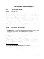
3.1 HYDAT DATABASE . . . . . . . . . . . . . . . . . . . . . . . . . . . . . . . . . . . . 171
3.1.1 Introduction . . . . . . . . . . . . . . . . . . . . . . . . . . . . . . . . . . . . . . . . 171
3.1.2 Accessing the Database . . . . . . . . . . . . . . . . . . . . . . . . . . . . . . 171
• To access the HYDAT database: . . . . . . . . . . . . . . . . . . . . . . . . . . . . . . 171
3.1.3
Accessing Station Details . . . . . . . . . . . . . . . . . . . . . . . . . . . . . 172
• To access a selected station: . . . . . . . . . . . . . . . . . . . . . . . . . . . . . . . . . 172
• To access a station by ID: . . . . . . . . . . . . . . . . . . . . . . . . . . . . . . . . . . . 173
3.1.4
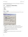
Properties of a HYDAT Station . . . . . . . . . . . . . . . . . . . . . . . . . 174
3.1.4.1
3.1.4.2
3.1.4.3
3.1.5
Details . . . . . . . . . . . . . . . . . . . . . . . . . . . . . . . . . . . . . . . . . . . . . 174
HYDEX . . . . . . . . . . . . . . . . . . . . . . . . . . . . . . . . . . . . . . . . . . . . . 175
Meta Data . . . . . . . . . . . . . . . . . . . . . . . . . . . . . . . . . . . . . . . . . . . 175
Properties of Associated Time Series . . . . . . . . . . . . . . . . . . . . 176
3.1.5.1
Subset . . . . . . . . . . . . . . . . . . . . . . . . . . . . . . . . . . . . . . . . . . . . . 177
3.2 CDCD DATABASE . . . . . . . . . . . . . . . . . . . . . . . . . . . . . . . . . . . . . 178
3.2.1 Introduction . . . . . . . . . . . . . . . . . . . . . . . . . . . . . . . . . . . . . . . . 178
3.2.2 Accessing the Database . . . . . . . . . . . . . . . . . . . . . . . . . . . . . . 178
• To access the CDCD database: . . . . . . . . . . . . . . . . . . . . . . . . . . . . . . . 178
3.2.3
Accessing Station Details . . . . . . . . . . . . . . . . . . . . . . . . . . . . . 179
• To access a selected station: . . . . . . . . . . . . . . . . . . . . . . . . . . . . . . . . . 179
• To access a station by ID: . . . . . . . . . . . . . . . . . . . . . . . . . . . . . . . . . . . 180
3.2.4
Properties of a CDCD Station . . . . . . . . . . . . . . . . . . . . . . . . . . 180
3.2.4.1
3.2.4.2
3.2.5
Details . . . . . . . . . . . . . . . . . . . . . . . . . . . . . . . . . . . . . . . . . . . . . 180
Meta Data . . . . . . . . . . . . . . . . . . . . . . . . . . . . . . . . . . . . . . . . . . . 181
Properties of Associated Time Series . . . . . . . . . . . . . . . . . . . . 181
3.2.5.1
Subset . . . . . . . . . . . . . . . . . . . . . . . . . . . . . . . . . . . . . . . . . . . . . 182
3.3 NARR DATABASE . . . . . . . . . . . . . . . . . . . . . . . . . . . . . . . . . . . . .
3.3.1 Introduction . . . . . . . . . . . . . . . . . . . . . . . . . . . . . . . . . . . . . . . .
3.3.2 Downloading the NARR Data . . . . . . . . . . . . . . . . . . . . . . . . . .
3.3.3 Accessing the NARR Variables . . . . . . . . . . . . . . . . . . . . . . . . .
184
184
184
185
• To import the NARR data: . . . . . . . . . . . . . . . . . . . . . . . . . . . . . . . . . . . 185
4
THE GEN1D MODEL . . . . . . . . . . . . . . . . . . . . . . . . . . . . . . 189
4.1 GENERAL BACKGROUND . . . . . . . . . . . . . . . . . . . . . . . . . . . . . . . . . .
4.1.1 Basic Equations . . . . . . . . . . . . . . . . . . . . . . . . . . . . . . . . . . . .
4.1.2 Geometric Requirements . . . . . . . . . . . . . . . . . . . . . . . . . . . . .
4.2 THE GEN1D INTERFACE . . . . . . . . . . . . . . . . . . . . . . . . . . . . . . . . . .
4.2.1 Setting Up Simulation Parameters . . . . . . . . . . . . . . . . . . . . . .
189
189
190
193
193
4.2.1.1 Simulation . . . . . . . . . . . . . . . . . . . . . . . . . . . . . . . . . . . . . . . . . . . 193
4.2.1.2 Channel . . . . . . . . . . . . . . . . . . . . . . . . . . . . . . . . . . . . . . . . . . . . 197
4.2.1.2.1 Creating a Channel Object . . . . . . . . . . . . . . . . . . . . . . . . . . . 197
• To create a new channel object: . . . . . . . . . . . . . . . . . . . . . . . . . . . . . . 197
xiii
EnSim Hydrologic
September 2007
4.2.1.2.2 Opening an Existing Channel Object . . . . . . . . . . . . . . . . . . . 198
• To open an existing channel object: . . . . . . . . . . . . . . . . . . . . . . . . . . . 198
4.2.1.2.3 Changing a Segment Attribute Value . . . . . . . . . . . . . . . . . . . 198
• To change a segment attribute value: . . . . . . . . . . . . . . . . . . . . . . . . . 198
4.2.1.2.4 Changing a Node Attribute Value . . . . . . . . . . . . . . . . . . . . . . 199
• To change a node’s attribute values: . . . . . . . . . . . . . . . . . . . . . . . . . . 199
• To change a node’s location or value: . . . . . . . . . . . . . . . . . . . . . . . . . 199
4.2.1.3 Down Boundary . . . . . . . . . . . . . . . . . . . . . . . . . . . . . . . . . . . . . .
4.2.1.4 Up Boundary . . . . . . . . . . . . . . . . . . . . . . . . . . . . . . . . . . . . . . . .
4.2.1.5 Cross-Sections . . . . . . . . . . . . . . . . . . . . . . . . . . . . . . . . . . . . . . .
4.2.1.5.1 Associating a Cross-Section with a Segment . . . . . . . . . . . . .
200
201
202
202
• To associate a cross-section with a segment: . . . . . . . . . . . . . . . . . . . 202
4.2.1.5.2 Scaling a Cross-Section . . . . . . . . . . . . . . . . . . . . . . . . . . . . . 203
• To scale a cross-section: . . . . . . . . . . . . . . . . . . . . . . . . . . . . . . . . . . . 203
4.2.1.5.3 Copying a Cross-section to a Segment . . . . . . . . . . . . . . . . . 203
• To copy a cross-section to a segment: . . . . . . . . . . . . . . . . . . . . . . . . . 203
4.2.1.5.4 Orthogonally Positioning a Cross-Section . . . . . . . . . . . . . . . 204
• To orthogonally position a cross-section: . . . . . . . . . . . . . . . . . . . . . . . 204
4.2.1.5.5 Resampling a Cross-Section . . . . . . . . . . . . . . . . . . . . . . . . . 204
• To resample a cross-section: . . . . . . . . . . . . . . . . . . . . . . . . . . . . . . . . 204
4.2.1.5.6 Interpolating a Cross-Section . . . . . . . . . . . . . . . . . . . . . . . . . 205
• To interpolate data from two cross-sections: . . . . . . . . . . . . . . . . . . . . 205
4.2.1.5.7 Vertically Offsetting a Cross-Section . . . . . . . . . . . . . . . . . . . 206
• To vertically offset a cross-section: . . . . . . . . . . . . . . . . . . . . . . . . . . . . 206
4.2.1.5.8 Generating a Simple Cross-Section . . . . . . . . . . . . . . . . . . . . 206
• To generate a simple cross-section: . . . . . . . . . . . . . . . . . . . . . . . . . . . 206
4.2.1.5.9 Removing a Cross-Section . . . . . . . . . . . . . . . . . . . . . . . . . . . 207
• To remove a cross-section: . . . . . . . . . . . . . . . . . . . . . . . . . . . . . . . . . 207
4.2.1.5.10Cross-Section Properties . . . . . . . . . . . . . . . . . . . . . . . . . . . . 207
• To view the properties of a cross-section: . . . . . . . . . . . . . . . . . . . . . . 207
4.2.2
Running the GEN1D Model . . . . . . . . . . . . . . . . . . . . . . . . . . . .208
• To run a GEN1D simulation: . . . . . . . . . . . . . . . . . . . . . . . . . . . . . . . . . 208
4.2.3
Displaying Simulation Output . . . . . . . . . . . . . . . . . . . . . . . . . . .208
4.2.3.1
Creating a Hot Start From an Output . . . . . . . . . . . . . . . . . . . . . . 209
• To extract a Hot Start from a GEN1D model run: . . . . . . . . . . . . . . . . . 209
5
THE HBV-EC MODEL . . . . . . . . . . . . . . . . . . . . . . . . . . . . . 211
5.1 GENERAL BACKGROUND . . . . . . . . . . . . . . . . . . . . . . . . . . . . . . . . . . .211
5.1.1 Background and History of the Model . . . . . . . . . . . . . . . . . . . .211
5.1.2 Algorithms Specific to the Model . . . . . . . . . . . . . . . . . . . . . . . .211
5.1.2.1
5.1.2.2
5.1.2.3
Climate Zones . . . . . . . . . . . . . . . . . . . . . . . . . . . . . . . . . . . . . . . 212
Snow Melt Factor Variation with Terrain Aspect and Slope . . . . . 212
Watershed Routing . . . . . . . . . . . . . . . . . . . . . . . . . . . . . . . . . . . 212
5.1.3 References . . . . . . . . . . . . . . . . . . . . . . . . . . . . . . . . . . . . . . . . .212
5.2 THE HBV-EC INTERFACE . . . . . . . . . . . . . . . . . . . . . . . . . . . . . . . . . .212
5.2.1 The EnSim WaterShed Panel . . . . . . . . . . . . . . . . . . . . . . . . . . .213
• To identify an alternate basin object: . . . . . . . . . . . . . . . . . . . . . . . . . . 215
5.2.2
xiv
The Basin Panel . . . . . . . . . . . . . . . . . . . . . . . . . . . . . . . . . . . . .216
Table of Contents
5.2.2.1
5.2.2.2
5.2.2.3
5.2.2.4
5.2.2.5
5.2.2.6
September 2007
The Climate Tab . . . . . . . . . . . . . . . . . . . . . . . . . . . . . . . . . . . . . .
The Elevation Tab . . . . . . . . . . . . . . . . . . . . . . . . . . . . . . . . . . . .
The Land Use Tab . . . . . . . . . . . . . . . . . . . . . . . . . . . . . . . . . . . .
The Slope Tab . . . . . . . . . . . . . . . . . . . . . . . . . . . . . . . . . . . . . . .
The Aspect Tab . . . . . . . . . . . . . . . . . . . . . . . . . . . . . . . . . . . . . .
Identifying Zones Within HBV-EC . . . . . . . . . . . . . . . . . . . . . . . .
216
217
218
219
220
221
• To identify a zone: . . . . . . . . . . . . . . . . . . . . . . . . . . . . . . . . . . . . . . . . . 221
5.2.3
5.2.4
The Simulation Panel . . . . . . . . . . . . . . . . . . . . . . . . . . . . . . . . 222
The Climate Zone Panel . . . . . . . . . . . . . . . . . . . . . . . . . . . . . . 225
5.2.4.1
5.2.4.2
5.3
The Parameters Tab . . . . . . . . . . . . . . . . . . . . . . . . . . . . . . . . . . 225
The Met Tab . . . . . . . . . . . . . . . . . . . . . . . . . . . . . . . . . . . . . . . . . 229
THE HBV-EC MODEL . . . . . . . . . . . . . . . . . . . . . . . . . . . . . . . . . . . . 231
• To run the HBV-EC model: . . . . . . . . . . . . . . . . . . . . . . . . . . . . . . . . . . 231
5.3.1
The Results of the HBV-EC Model . . . . . . . . . . . . . . . . . . . . . . 232
APPENDIX A:FILE TYPES OF ENSIM CORE . . . . . . . . . . . . . . 235
General Information . . . . . . . . . . . . . . . . . . . . . . . . . . . . . . . . . 235
File Headers . . . . . . . . . . . . . . . . . . . . . . . . . . . . . . . . . . . . . . . 236
ASCII and Binary Files . . . . . . . . . . . . . . . . . . . . . . . . . . . . . . . 240
ASCII Files . . . . . . . . . . . . . . . . . . . . . . . . . . . . . . . . . . . . . . . . . . 240
Binary Files . . . . . . . . . . . . . . . . . . . . . . . . . . . . . . . . . . . . . . . . . . 240
NATIVE FILE FORMATS . . . . . . . . . . . . . . . . . . . . . . . . . . . . . . . . . . . . 242
2D Rectangular Grids [r2s / r2v] . . . . . . . . . . . . . . . . . . . . . . . . 242
File Headers [r2s / r2v] . . . . . . . . . . . . . . . . . . . . . . . . . . . . . . . . .
Data Organization [r2s / r2v] . . . . . . . . . . . . . . . . . . . . . . . . . . . .
File Formats [r2s / r2v] . . . . . . . . . . . . . . . . . . . . . . . . . . . . . . . . .
ASCII . . . . . . . . . . . . . . . . . . . . . . . . . . . . . . . . . . . . . . . . . . .
Binary . . . . . . . . . . . . . . . . . . . . . . . . . . . . . . . . . . . . . . . . . . .
242
243
243
244
244
2D Triangular Meshes [t3s / t3v] . . . . . . . . . . . . . . . . . . . . . . . . 246
File Headers [t3s / t3v] . . . . . . . . . . . . . . . . . . . . . . . . . . . . . . . . .
File Formats [t3s / t3v] . . . . . . . . . . . . . . . . . . . . . . . . . . . . . . . . .
ASCII . . . . . . . . . . . . . . . . . . . . . . . . . . . . . . . . . . . . . . . . . . .
Binary . . . . . . . . . . . . . . . . . . . . . . . . . . . . . . . . . . . . . . . . . . .
246
247
247
248
Line Sets [i2s / i3s] . . . . . . . . . . . . . . . . . . . . . . . . . . . . . . . . . . 250
File Headers [i2s / i3s] . . . . . . . . . . . . . . . . . . . . . . . . . . . . . . . . .
File Formats [i2s / i3s] . . . . . . . . . . . . . . . . . . . . . . . . . . . . . . . . .
ASCII . . . . . . . . . . . . . . . . . . . . . . . . . . . . . . . . . . . . . . . . . . .
Binary . . . . . . . . . . . . . . . . . . . . . . . . . . . . . . . . . . . . . . . . . . .
250
251
251
251
XYZ Point Sets [xyz] . . . . . . . . . . . . . . . . . . . . . . . . . . . . . . . . . 252
File Headers [xyz] . . . . . . . . . . . . . . . . . . . . . . . . . . . . . . . . . . . . . 252
File Format [xyz] . . . . . . . . . . . . . . . . . . . . . . . . . . . . . . . . . . . . . . 252
XY Data Objects [xy] [dat] . . . . . . . . . . . . . . . . . . . . . . . . . . . . . 253
File Headers [xy] [dat] . . . . . . . . . . . . . . . . . . . . . . . . . . . . . . . . . 253
File Format [xy] [dat] . . . . . . . . . . . . . . . . . . . . . . . . . . . . . . . . . . . 253
Parcel Sets [pcl] . . . . . . . . . . . . . . . . . . . . . . . . . . . . . . . . . . . . 254
xv
EnSim Hydrologic
September 2007
File Headers [pcl] . . . . . . . . . . . . . . . . . . . . . . . . . . . . . . . . . . . . .
File Formats [pcl] . . . . . . . . . . . . . . . . . . . . . . . . . . . . . . . . . . . . .
ASCII . . . . . . . . . . . . . . . . . . . . . . . . . . . . . . . . . . . . . . . . . . .
Binary . . . . . . . . . . . . . . . . . . . . . . . . . . . . . . . . . . . . . . . . . . .
254
255
255
255
Point Sets [pt2] . . . . . . . . . . . . . . . . . . . . . . . . . . . . . . . . . . . . . .256
File Headers [pt2] . . . . . . . . . . . . . . . . . . . . . . . . . . . . . . . . . . . . . 256
File Formats [pt2] . . . . . . . . . . . . . . . . . . . . . . . . . . . . . . . . . . . . . 257
ASCII . . . . . . . . . . . . . . . . . . . . . . . . . . . . . . . . . . . . . . . . . . . 257
Time Series [ts1 / ts2 / ts3 / ts4 / ts5] . . . . . . . . . . . . . . . . . . . . .258
File Headers [ts1 / ts2 / ts3 / ts4] . . . . . . . . . . . . . . . . . . . . . . . . .
File Headers [ts5] . . . . . . . . . . . . . . . . . . . . . . . . . . . . . . . . . . . . .
File Formats [ts1 / ts2 / ts3 / ts4 / ts5] . . . . . . . . . . . . . . . . . . . . .
ASCII . . . . . . . . . . . . . . . . . . . . . . . . . . . . . . . . . . . . . . . . . . .
Binary . . . . . . . . . . . . . . . . . . . . . . . . . . . . . . . . . . . . . . . . . . .
258
259
260
260
262
Tables [tb0] . . . . . . . . . . . . . . . . . . . . . . . . . . . . . . . . . . . . . . . . .263
File Headers [tb0 ] . . . . . . . . . . . . . . . . . . . . . . . . . . . . . . . . . . . .
File Format [tb0] . . . . . . . . . . . . . . . . . . . . . . . . . . . . . . . . . . . . . .
ASCII . . . . . . . . . . . . . . . . . . . . . . . . . . . . . . . . . . . . . . . . . . .
Binary . . . . . . . . . . . . . . . . . . . . . . . . . . . . . . . . . . . . . . . . . . .
263
264
264
264
Velocity Roses [vr1] . . . . . . . . . . . . . . . . . . . . . . . . . . . . . . . . . .265
File Headers [vr1] . . . . . . . . . . . . . . . . . . . . . . . . . . . . . . . . . . . . . 265
File Formats [vr1] . . . . . . . . . . . . . . . . . . . . . . . . . . . . . . . . . . . . . 265
ASCII . . . . . . . . . . . . . . . . . . . . . . . . . . . . . . . . . . . . . . . . . . . 265
Networks [n3s] . . . . . . . . . . . . . . . . . . . . . . . . . . . . . . . . . . . . . .266
File Headers [n3s] . . . . . . . . . . . . . . . . . . . . . . . . . . . . . . . . . . . .
File Formats [n3s] . . . . . . . . . . . . . . . . . . . . . . . . . . . . . . . . . . . .
ASCII . . . . . . . . . . . . . . . . . . . . . . . . . . . . . . . . . . . . . . . . . . .
Binary . . . . . . . . . . . . . . . . . . . . . . . . . . . . . . . . . . . . . . . . . . .
266
267
267
268
SUPPORTED FOREIGN FILE FORMATS [ENSIM CORE] . . . . . . . . . . . . . .270
GeoTIFF Theme files [thm] . . . . . . . . . . . . . . . . . . . . . . . . . . . . .271
APPENDIX B:FILE TYPES OF ENSIM HYDROLOGIC . . . . . . . 273
NATIVE FILE TYPES . . . . . . . . . . . . . . . . . . . . . . . . . . . . . . . . . . . . . . .274
Watershed Objects [wsd] . . . . . . . . . . . . . . . . . . . . . . . . . . . . . .274
File Headers [wsd] . . . . . . . . . . . . . . . . . . . . . . . . . . . . . . . . . . . .
File Format [wsd] . . . . . . . . . . . . . . . . . . . . . . . . . . . . . . . . . . . . .
ASCII . . . . . . . . . . . . . . . . . . . . . . . . . . . . . . . . . . . . . . . . . . .
Binary . . . . . . . . . . . . . . . . . . . . . . . . . . . . . . . . . . . . . . . . . . .
274
276
276
276
2D Rectangular Cell Grids [r2c] . . . . . . . . . . . . . . . . . . . . . . . . .277
File Headers [r2c] . . . . . . . . . . . . . . . . . . . . . . . . . . . . . . . . . . . . .
File Formats [r2c] . . . . . . . . . . . . . . . . . . . . . . . . . . . . . . . . . . . . .
ASCII . . . . . . . . . . . . . . . . . . . . . . . . . . . . . . . . . . . . . . . . . . .
Multiframe ASCII . . . . . . . . . . . . . . . . . . . . . . . . . . . . . . . . . .
Binary . . . . . . . . . . . . . . . . . . . . . . . . . . . . . . . . . . . . . . . . . . .
xvi
277
278
278
279
279
Table of Contents
September 2007
SUPPORTED FOREIGN FILE TYPES [ENSIM HYDROLOGIC] . . . . . . . . . . 281
APPENDIX C:FILE TYPES OF THE RCA . . . . . . . . . . . . . . . . . 283
The Rating Curve Analysis File [rca] . . . . . . . . . . . . . . . . . . . . . 283
File Header [rca] . . . . . . . . . . . . . . . . . . . . . . . . . . . . . . . . . . . . . .
File Format [rca] . . . . . . . . . . . . . . . . . . . . . . . . . . . . . . . . . . . . . .
ASCII . . . . . . . . . . . . . . . . . . . . . . . . . . . . . . . . . . . . . . . . . . .
Binary . . . . . . . . . . . . . . . . . . . . . . . . . . . . . . . . . . . . . . . . . . .
283
284
284
284
APPENDIX D:FILE TYPES OF GEN1D . . . . . . . . . . . . . . . . . . . 285
The GEN1D Parameter File . . . . . . . . . . . . . . . . . . . . . . . . . . . 285
File Header [g1d] . . . . . . . . . . . . . . . . . . . . . . . . . . . . . . . . . . . . .
File Format [g1d] . . . . . . . . . . . . . . . . . . . . . . . . . . . . . . . . . . . . .
Simulation Parameters . . . . . . . . . . . . . . . . . . . . . . . . . . . . . . . . .
General Parameters . . . . . . . . . . . . . . . . . . . . . . . . . . . . . . . .
Simulation Parameters . . . . . . . . . . . . . . . . . . . . . . . . . . . . . .
Constants . . . . . . . . . . . . . . . . . . . . . . . . . . . . . . . . . . . . . . . .
Input Files . . . . . . . . . . . . . . . . . . . . . . . . . . . . . . . . . . . . . . . .
Boundaries . . . . . . . . . . . . . . . . . . . . . . . . . . . . . . . . . . . . . . .
Output . . . . . . . . . . . . . . . . . . . . . . . . . . . . . . . . . . . . . . . . . . .
285
285
286
286
286
287
289
289
291
APPENDIX E:FILE TYPES OF HBV-EC . . . . . . . . . . . . . . . . . . 293
The HBV-EC Parameter Set File . . . . . . . . . . . . . . . . . . . . . . . 293
File Header [hbv] . . . . . . . . . . . . . . . . . . . . . . . . . . . . . . . . . . . . . 293
File Format [hbv] . . . . . . . . . . . . . . . . . . . . . . . . . . . . . . . . . . . . . 296
The HBV-EC MET file . . . . . . . . . . . . . . . . . . . . . . . . . . . . . . . . 297
File Header [met] . . . . . . . . . . . . . . . . . . . . . . . . . . . . . . . . . . . . . 297
File Format [met] . . . . . . . . . . . . . . . . . . . . . . . . . . . . . . . . . . . . . 298
xvii
EnSim Hydrologic
xviii
September 2007
1
ENSIM CORE
1.1
A QUICK OVERVIEW
1.1.1
The EnSim Simulation Environment
Developed at the Canadian Hydraulics Centre (CHC), EnSim was created to meet the needs of
a wide range of environmental prediction and decision support systems. EnSim is designed as
an advanced numerical modelling environment, as well as a general purpose data handling and
visualisation system that can easily be adapted for any class of environmental data.
EnSim provides an ideal framework for the integration of environmental data, GIS information
and model data. An EnSim application can be designed to run a simple numerical model or a
suite of numerical models providing a variety of pre- and post-processing tools. It is designed
as a generic toolkit from which a system developer chooses components to create an
application.
For the modeller, EnSim creates a virtual environment where simulation results can be viewed,
animated and analyzed in one, two and three dimensions. This allows you to observe complex
interactions of various phenomena in an intuitive manner, providing a realistic view of
simulation results.
Presentation of simulation results to non-technical audiences can be greatly improved by
providing seamless integration with other Windows applications such as word-processors,
spreadsheets and multimedia tools.
1.1.2
Getting Started
EnSim Core forms the basis of a variety of applications (e.g. WaveSim, EnSim Telemac,
EnSim Hydrologic) that comprise the EnSim family. These applications all share fundamental
functions, which form the core of EnSim. As a result, this EnSim manual is set up in a modular
fashion. There is a section under the heading "EnSim Core" that details the functions common
to all EnSim applications, and a separate section, under the title of the application, that
describes those functions that are particular to the specific EnSim application.
As a first time user, it might be easier to begin with the section on EnSim Core to become
familiar with the basics of EnSim before proceeding to the section which is specific to the
EnSim application. The sections of this manual that are specific to a particular application
illustrate how to perform only the functions that are specific to that application (e.g. EnSim
Telemac) and assume that you are familiar with core EnSim functions.
1
EnSim Core
1.1.3
September 2007
Getting Help with EnSim
EnSim is a Windows-based application. All EnSim documentation assumes that you are
familiar with Windows-based applications. That is, it assumes you know how to use a mouse,
open a menu, choose menu and dialog options, and other Windows-based functions. EnSim
documentation also assumes familiarity with standard Windows menus and buttons, such as the
Open document command, which can be found in the File menu or by clicking the
button.
Consult your Windows documentation for help in using Windows-based applications.
EnSim documentation consists of a manual and an online help system. The online help system
is accessed through the EnSim Help menu. The manual and the online help system of EnSim
documentation are intended to be independent. All information contained in the manual can
also be found in the online help system. Version and copyright information about EnSim can
be obtained using the command About... in the Help menu.
1.1.3.1
Conventions in EnSim Help
Bold designates the name of a menu, menu choice, dialog, dialog option, or workspace
category.
e.g. File
Italics highlight a term or concept being defined or described.
e.g. Categories are elements defined by EnSim to organise the workspace.
<Angle brackets> indicate key presses.
e.g. <Ctrl> key
An “→“ indicates a sequence of menu selections.
e.g. File→Open
2
Section 1.2: The WorkSpace
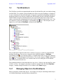
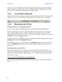
1.2
September 2007
THE WORKSPACE
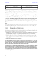
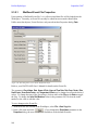
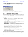
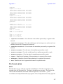
The WorkSpace provides an organizational structure for the data files and view windows being
used in EnSim. In a window on the left-hand side of the screen, the WorkSpace is displayed
as a tree consisting of a hierarchical display of categories (organizational headings for objects)
and objects (data or view objects), similar to the file hierarchy structure of Windows Explorer.
Unlike Windows Explorer, the hierarchy does not represent the physical location of files;
rather, it represents the relationship between the objects and between objects and views. The
top of the tree is always the WorkSpace, represented by the icon. The workspace can be
toggled on or off using the WorkSpace command in the View menu.
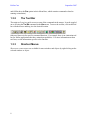
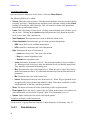
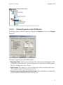
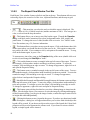
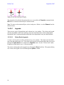
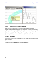
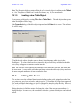
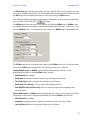
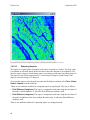
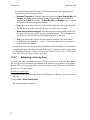
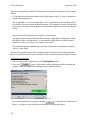
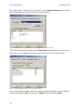
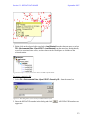
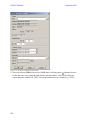
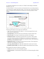
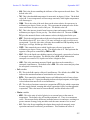
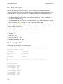
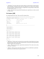
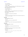
Figure 1.1: The EnSim WorkSpace includes Data Items and Views
The second branch of the hierarchical tree consists of categories, which are organizational
headings for objects. There are two categories in the EnSim WorkSpace. Data Items,
represented by the icon, is the first category. It contains all the files, or data items, that have
been opened or created during the EnSim session. The second category is Views, represented
by the icon. It contains all the view windows that are active during the session and the
objects associated with each view.
The remaining branches of the hierarchical tree are objects. Objects can represent files, parts
of a file, or views. An example of an object would be a model results file in the Data Items
category. Another example would be a view window in the Views category.
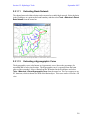
1.2.1
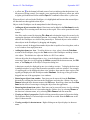
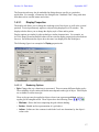
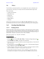
Managing Objects in the WorkSpace
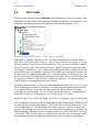
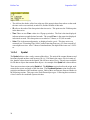
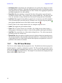
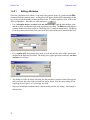
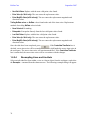
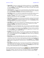
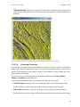
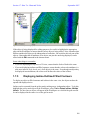
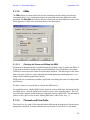
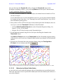
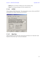
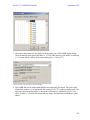
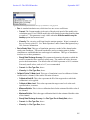
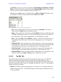
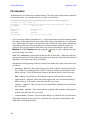
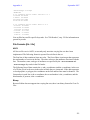
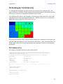
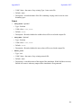
Objects sometimes contain other objects. An example of an object containing another object
is an EnSim Hydrologic watershed object, shown below.
3
EnSim Core
September 2007
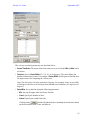
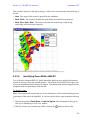
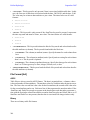
Figure 1.2: An EnSim Hydrologic watershed object contains other objects
The three objects under the Test Watershed object are considered children of the parent object.
Other examples of objects that are shown as children are extracted time series and 3D line sets.
The children, or components, of an object can be displayed or hidden in the workspace by
clicking on the + or - signs, respectively, located to the left of the object. In many cases, only
the children of an object can be dragged into a view. If a child was created from a viewable
parent object, such as a time series extraction from a triangular mesh, then both the child and
parent can be displayed.
Objects in the WorkSpace are represented by icons, which indicate the object’s type, and
therefore, some of the object’s properties. Icons for some common data items are detailed
below. Details concerning each type of data file can be found in the Appendices.
a file, usually a container file for other objects
rectangular grid, scalar data
rectangular grid, vector data
triangular mesh, scalar data
triangular mesh, vector data
2-dimensional line set (for example, isolines or GIS data)
3-dimensional line set
network file (describes a network of segments and nodes)
xy data item
time series, scalar
time series, vector
point set
geoTIFF image
table
There are a few icon decorations that indicate the status of an object:
• a black square
• a red square
• a red circle
4
indicates that a data item is in a view window.
indicates that animation is activated on an object in a view window.
indicates an empty object, which contains no data
Section 1.2: The WorkSpace
September 2007
• a yellow star in the bottom left-hand corner of an icon indicates that the data item is in
the process of being created. For example, a new regular grid will have a yellow star, while
a regular grid loaded into EnSim with the Open file command will not have a yellow star.
When an object is selected in the WorkSpace, it is highlighted and becomes the current object.
All functions are then applied to that object.
Objects in the WorkSpace can be manipulated in the following ways:
• Adding an object to another object. Data items can be added to the Data Items hierarchy
by opening a file or creating a new data item, such as a grid. Files can be opened in the same
manner.
New files can be created by choosing File→New and selecting the item to be created, or by
creating the data item with an EnSim function. For example, when a 3D line is created, it is
added to the WorkSpace as a child of the parent object. Selected objects can be added to
other objects in the WorkSpace by dragging and dropping.
An object can only be dragged into another object that is capable of receiving data, such as
a view window or an empty data item.
• Adding data items to a view. To add an object to a view, select it from the Data Items
section of the WorkSpace, drag it to the View section of the WorkSpace and drop it into a
view object. The default view object in EnSim is a 2D View window.
After an object has been dropped into a view, it can be displayed or hidden without
removing it from the view by toggling the Visible command in the shortcut menu, the Edit
menu, or the Display tab of the object’s Properties dialog box.
A data item can only be displayed in one view window at a time. To display the data item
in multiple windows, a copy of the file must be opened for each view window. For example,
if a regular grid is to be displayed in three view windows, there must be three copies of the
regular grid displayed in the WorkSpace under Data Items. Each copy of the grid is then
dropped into one of the appropriate view windows.
• Removing an object from another. Data items can be removed from the Data Items
hierarchy by selecting the data item in the WorkSpace and using the <Delete> key or the
Remove command in the shortcut menu or the Edit menu. Removing a data item from Data
Items has the effect of removing or closing the object from the application.
• Removing data items from a view. Data items can be removed from a view by selecting
the data item within the list of views and using the <Delete> key, by selecting Remove in
the data item’s shortcut menu, or by selecting Edit→Remove from the menu bar.
• Viewing an Object’s properties. Double clicking on an object opens its Properties dialog.
The Properties dialog of a selected object can also be accessed from the Edit menu or the
object’s shortcut menu.
• Viewing an object’s shortcut menu. Right-clicking on an object displays its shortcut
menu.
5
EnSim Core
September 2007
• Renaming an object. After opening the Properties dialog, select the Meta Data tab and
change the text in the Title or Name fields. The Title field will change the name of the object
at the top of the Properties dialog box, while the Name field will change the name of the
object in the WorkSpace, data probes, and the automatic title of the colour-scale legend.
1.2.2
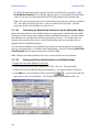
Saving and Loading The WorkSpace
EnSim allows you to save the current state of the WorkSpace to an EnSim WorkSpace File
(*.ews). The EnSim WorkSpace File contains all the data item settings, including colour
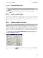
scales, legend options, scaling, rendering options, line width, point size, and so on, for all
currently opened objects. As well as saving data item settings, it also saves the settings for all
the views and the object view relationships. This ASCII file should not be edited directly.
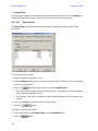
To Save a WorkSpace:
1. On the menu bar, select File→Save WorkSpace....
2. When the Save Current WorkSpace As dialog appears, enter an appropriate name and click
.
3. The WorkSpace can only be saved if all objects have a file association. Extracted isolines,
time series, new Point Sets, new Line Sets, etc. do not have such an association when first
created. If any of the objects within the WorkSpace need to be saved, you will be prompted
to do so. Click Yes to save the objects, or No to cancel the Save WorkSpace operation.
1. Give each of the objects an appropriate name and click
to save them. If you
click
for any object, the Save WorkSpace operation will be cancelled, but any
objects already saved will remain saved.
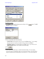
To Load a WorkSpace:
Note: Loading an EnSim Workspace file will remove any existing objects or views from the
EnSim environment. If necessary, make sure that you’ve saved the current WorkSpace.
EnSim WorkSpace files created by a EnSim application can be loaded by that EnSim
application only. The files are not compatible in any other EnSim application.
1. Select File→Load WorkSpace from the menu bar.
2. When prompted to continue, select the
button. The current WorkSpace will be
cleared. If the
button is selected, no changes will be made to the current
WorkSpace.
2. In the Open dialog, select the desired EnSim WorkSpace File and select the
button.
6
Section 1.3: The EnSim Interface
1.3
September 2007
THE ENSIM INTERFACE
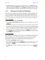
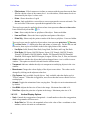
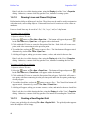
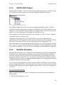
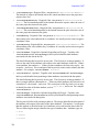
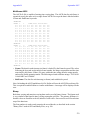
The interface is customized for specific applications as necessary. The basic graphical user
interface consists of four main components: a menu bar and a tool bar, both for selecting
various windows and EnSim functions; a workspace, for managing open data files and views;
and an area for various views (i.e., 1D, Polar, 2D, 3D, Spherical, and Report).
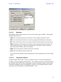
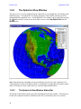
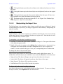
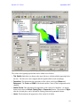
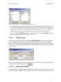
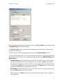
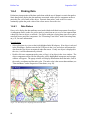
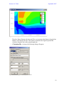
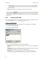
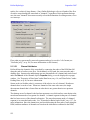
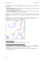
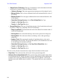
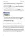
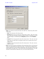
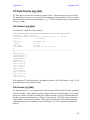
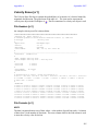
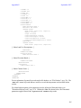
An example of the basic EnSim interface follows. The title bar identifies this interface as being
from WaveSim. However, most EnSim applications have the same basic interface and will
look similar to this example.
Figure 1.3: The EnSim interface window
1.3.1
The Menu Bar
The menu bar consists of the standard Windows options: File, Edit, View, Tools, Window, and
Help.
Commands in these menus that are specific to EnSim will be detailed in the appropriate
sections. Specific EnSim applications may contain other menus in the menu bar (e.g. WaveSim
7
EnSim Core
September 2007
and OilSim have the Run option in their Menu Bars, which contains commands related to
running a simulation).
1.3.2
The Tool Bar
The main tool bar gives quick access to some of the commands in the menus. It can be toggled
on or off using the Tool Bar command in the View menu. To move the tool bar, click on the tool
bar with the mouse and drag it to the desired location.
Other tool bars exist for specific command functions. For example, there is an Animation tool
bar for EnSim applications that have animation capabilities. For more information on these
tool bars, see the information specific to the function.
1.3.3
Shortcut Menus
Shortcut or context menus are available for most windows and objects by right clicking on the
selected window or object.
8
Section 1.4: Data Items
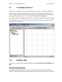
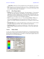
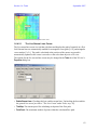
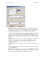
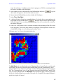
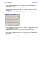
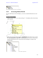
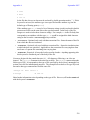
1.4
September 2007
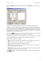
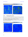
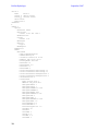
DATA ITEMS
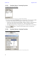
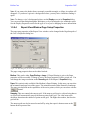
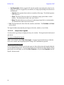
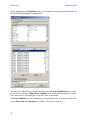
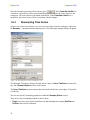
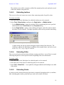
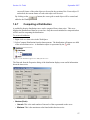
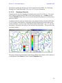
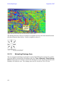
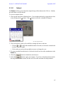
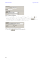
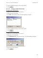
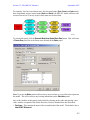
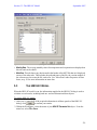
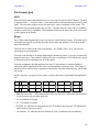
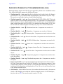
The items listed under the category Data Items in the WorkSpace are referred to as objects. The
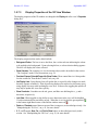
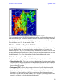
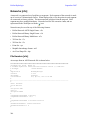
following is an image of an EnSim Hydrologic WorkSpace displaying various objects (i.e. the
'Jock River' watershed object, the 'Rectangular Grid', the 'Basin 8 boundary', etc.).
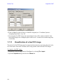
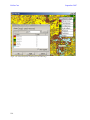
Figure 1.4: The EnSim Hydrologic WorkSpace contains several types of Data Items
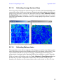
Each object is a coherent collection of data. The data contained within a particular type of
object may come from a variety of sources. Take a 2D line set object, for example. A 2D line
set object consists of one or more 2-dimensional lines. The geometry of each line is defined
by two or more xy points. Each line may also have a number of attributes associated with it.
For example, if the line set is a set of isolines representing contour data, each line will have an
associated elevation. The data that comprises a line set object may come from, for instance, an
ArcInfo shape file, a MapInfo interchange file, or an EnSim native i2s (2D line set) file. The
organization of data is quite different in each of these source files. However, the data from each
are organized in EnSim as a line set object. EnSim uses objects as a way of taking data in
various formats, and putting them in a uniform format.
All objects of the same type (e.g. line sets, 2D Rectangular scalar grids, point sets, etc.) can be
used and displayed in the same way and they can all have the same functions applied to them.
For example, all line set objects have the same options for display, and can be used in
performing the same functions. The same display options and functions are not necessarily
applicable to an object of a different type, say a 2D grid object or a point set.
All EnSim objects have a native file format. See "Native File Formats", on p. 242, for details.
There are different categories of objects: spatial objects and container objects. Spatial objects
are those that have geometry and attributes. They are the ones that can be displayed in a view,
edited, manipulated, etc. Container objects do not have geometry. They are containers or
organizers for other objects and data. They keep related objects together in one location. An
EnSim Hydrologic Watershed object is a container, and so is an EnSim TELEMAC SELAFIN
(*.slf) object. Time series are similar to spatial objects in that they may be displayed, edited,
and manipulated, but they are different in that they do not have geometry, only attributes.
9
EnSim Core
1.4.1
September 2007
Loading and Importing Data Items
To load a data item into the WorkSpace, there are two types of data items recognized by EnSim:
1. For native EnSim data items, choose the Open command from the File menu, or use the
button. When the Open dialog box appears, select the file to be opened into the WorkSpace
and choose the
button. The 8 files most recently opened in EnSim are shown
at the bottom of the File menu.
2. For foreign data items, choose the Import command from the File menu. When the Open
dialog appears, select the file and choose the
button.
1.4.1.1
Native Data Items
The data items that are recognized by all EnSim applications are:
2D Rectangular Scalar Grids: Two-dimensional rectangular or regular grid having evenly
spaced nodes in both dimensions. X-spacing may differ from y-spacing. The node values of
the grid are scalar quantities (e.g. Elevation, concentration etc.) associated with each node.
May be time-varying.
2D Rectangular Vector Grid: Two-dimensional rectangular or regular grid having evenly
spaced nodes in both dimensions. X-spacing may differ from y-spacing. The node values of
the grid are vector quantities (e.g. velocity). May be time-varying.
2D Triangular Scalar Mesh: Two-dimensional triangular mesh. The node values of the mesh
are scalar quantities (e.g. elevation, concentration etc.) associated with each node. May be
time-varying.
2D Triangular Vector Mesh: Two-dimensional triangular mesh. The node values of the mesh
are vector quantities (e.g. velocity.) associated with each node. May be time-varying.
2D Line Sets: Open or closed collection of lines defined by two-dimensional nodes. Each line
may have multiple associated attributes. For example, if the lines are contour lines it may
include elevation data. Attributes may be integer, float, text, etc. See "Line Sets [i2s / i3s]",
on p. 250, for further details.
3D Line Sets: Open or closed collection of lines defined by three-dimensional nodes. Each
line may have multiple associated attributes. For example, if the lines are contour lines it may
include elevation data. Attributes may be integer, float, text, etc. See "Line Sets [i2s / i3s]",
on p. 250, for further details.
Point Sets: Set of points, each represented by an x and y coordinate. Each point may have
multiple associated attributes.
XYZ Point Sets: Set of points, each represented by an x, y, and z coordinate.
Parcel Sets: Set of points, each represented by an x, y, and z coordinate. May have multiple
attributes, and may be time-varying. Location of points may move if they vary over time.
10
Section 1.4: Data Items
September 2007
XY Data Sets: Set of scalar pairs. Each pair represents values from two attributes, attribute X
and attribute Y.
Scalar Implicit Time Series: Represents a scalar quantity varying with a simple time step in
seconds extracted from an x and y location.
Vector Implicit Time Series: Represents a vector quantity varying with a simple time step in
seconds extracted from an x and y location.
Scalar Explicit Time Series: Represents a scalar quantity varying with an explicit data and
time extracted from an x and y location.
Vector Explicit Time Series: Represents a vector quantity varying with an explicit data and
time extracted from an x and y location.
Networks: A set of interconnected polylines or segments. Each segment is made up of a series
of 3D vertices, and may have multiple attributes (e.g. roads, channels).
Tables: A set of data values organized into rows and columns. Columns represent the
attributes and rows represent the values at each attribute index.
Velocity Roses: Represents probabilities of vector quantities tabulated by magnitude and
direction.
1.4.1.2
Foreign Data Items
Please refer to "Supported Foreign File Formats [EnSim Core]", on p. 270, for further details.
1.4.2
Saving and Exporting Data Items
To save a data item to a file, select the object in the WorkSpace. To save the current object,
choose the Save command from the File menu or use the
button. A copy of the object may
be saved with the Save Copy As... command from the File menu. When the Save Copy As...
command is used, a copy of the current object is saved. This command is used to save a
back-up copy of an object and then to continue to edit the original object, or to export the object
to another file format.
All data items, regardless of their source, can be saved in at least one of the native EnSim file
formats. The format in which the object may be saved depends on the type of data. Click on
the
button or choose Save or Save Copy As... option from the File menu. Use the Save as
type box at the bottom of the dialog window to view the various file formats in which the object
may be saved. See Appendix A for a complete description of the native file formats.
The data items and the file formats in which they may be saved are as follows:
Icon
Object Type
Point Set
May Be Saved As...
.pt2 - ASCII (EnSim format)
11
EnSim Core
Icon
September 2007
Object Type
May Be Saved As...
.xyz - ASCII (EnSim format)
ArcView Shape (.shp)
MapInfo Interchange Format (.mif)
XYZ Point Set
.xyz - ASCII (EnSim format)
ArcView Shape (.shp)
MapInfo Interchange Format (.mif)
Parcel Set
.pcl - Lagrangian parcel set (EnSim format)
ArcView Shape (.shp)
MapInfo Interchange Format (.mif)
Multi-frame MapInfo (.mif)
XY Data Items
.xy or .dat ASCII (EnSim format)
2D Rectangular Scalar Grid
.r2s - ASCII Single Frame (EnSim format)
.r2s - Binary Single Frame (EnSim format)
.r2s - Binary Multi Frame (EnSim format)
.t3s - ASCII Single Frame (EnSim format)
.t3s - Binary Multi Frame (EnSim format)
.xyz - ASCII (EnSim format)
.grd - Surfer Grid
.asc - ArcInfo ASCII Grid
2D Rectangular Vector Grid
.r2v - ASCII Single Frame (EnSim format)
.r2v - Binary Single Frame (EnSim format)
.r2v - Binary Multi Frame (EnSim format)
.r2s - ASCII Magnitude (EnSim format)
.r2s - Binary Magnitude (EnSim format)
.t3v - ASCII Single Frame (EnSim format)
.t3v - Binary Multi Frame (EnSim format)
2D Triangular Scalar Mesh
12
.t3s - ASCII (EnSim format)
Section 1.4: Data Items
Icon
Object Type
September 2007
May Be Saved As...
.t3s - Binary Single Frame (EnSim format)
.t3s - Binary Multi Frame (EnSim format)
.xyz - Magnitude (EnSim format)
2D Triangular Vector Mesh
.t3v - ASCII (EnSim format)
.t3v - Binary Single Frame (EnSim format)
.t3v - Binary Multi Frame (EnSim format)
.t3s - ASCII magnitude only (EnSim format)
.t3s - Binary magnitude only (EnSim format)
.xyz - ASCII magnitude only (EnSim format)
Network
.n3s - ASCII (EnSim format)
.n3s - Binary Single Frame (EnSim format)
.n3s - Binary Multi Frame (EnSim format)
.i3s - ASCII (EnSim format)
.i2s - ASCII (EnSim format)
.xyz ASCII (EnSim format)
ArcView Shape (.shp)
MapInfo Interchange Format (.mif)
Time Series Type 1
.ts1 - ASCII (EnSim format)
.ts3 - ASCII (EnSim format)
Time Series Type 3
.ts3 - ASCII (EnSim format)
Time Series Type 2
.t2s - ASCII Mag. and Dir. (EnSim format)
.t2s - ASCII U and V (EnSim format)
.t4s - ASCII Mag. and Dir. (EnSim format)
.t4s - ASCII U and V (EnSim format)
Time Series Type 4
.t4s - ASCII Mag. and Dir. (EnSim format)
.t4s - ASCII U and V (EnSim format)
2D LineSets
.i2s - ASCII (EnSim format)
13
EnSim Core
September 2007
Icon
Object Type
May Be Saved As...
.i3s - ASCII (EnSim format)
.xyz - ASCII (EnSim format)
ArcView Shape (.shp)
MapInfo Interchange Format (.mif)
3D LineSets
.i3s - ASCII (EnSim format)
.i2s - ASCII (EnSim format)
.xyz - ASCII (EnSim format)
.xy - ASCII distance value (EnSim format)
ArcView Shape (.shp)
MapInfo Interchange Format (.mif)
Tables
.tb0 - Table Data (EnSim format)
.csv - Comma Delimited text
Velocity Rose
.vr1 - ASCII (EnSim format)
ArcView Shape Files
None *
MapInfo Interchange Format
None †
GeoTIFF
tiff - GeoTIFF ‡
Surfer Grid
.r2s - ASCII Single Frame (EnSim format)
.r2s - Binary Single Frame (EnSim format)
.r2s - Binary Multi Frame (EnSim format)
.t3s - ASCII Single Frame (EnSim format)
.t3s - Binary Multi Frame (EnSim format)
.xyz - ASCII (EnSim format)
.grd - Surfer Grid
.asc - ArcInfo ASCII Grid
DEM (DTED & CDED)
.r2s - ASCII Single Frame (EnSim format)
.r2s - Binary Single Frame (EnSim format)
.r2s - Binary Multi Frame (EnSim format)
14
Section 1.4: Data Items
Icon
Object Type
September 2007
May Be Saved As...
.t3s - ASCII Single Frame (EnSim format)
.t3s - Binary Multi Frame (EnSim format)
.xyz - ASCII (EnSim format)
.grd - Surfer Grid
.asc - ArcInfo ASCII Grid
ArcInfo ASCII Grid
.r2s - ASCII Single Frame (EnSim format)
.r2s - Binary Single Frame (EnSim format)
.r2s - Binary Multi Frame (EnSim format)
.t3s - ASCII Single Frame (EnSim format)
.t3s - Binary Multi Frame (EnSim format)
.xyz - ASCII (EnSim format)
.grd - Surfer Grid
.asc - ArcInfo ASCII Grid
Binary Raster
.r2s - ASCII Single Frame (EnSim format)
.r2s - Binary Single Frame (EnSim format)
.r2s - Binary Multi Frame (EnSim format)
.t3s - ASCII Single Frame (EnSim format)
.t3s - Binary Multi Frame (EnSim format)
.xyz - ASCII (EnSim format)
.grd - Surfer Grid
.asc - ArcInfo ASCII Grid
SRTM1 & SRTM3
.r2s - ASCII Single Frame (EnSim format)
.r2s - Binary Single Frame (EnSim format)
.r2s - Binary Multi Frame (EnSim format)
.t3s - ASCII Single Frame (EnSim format)
.t3s - Binary Multi Frame (EnSim format)
.xyz - ASCII (EnSim format)
.grd - Surfer Grid
15
EnSim Core
Icon
September 2007
Object Type
May Be Saved As...
.asc - ArcInfo ASCII Grid
Note:
* ArcView Shape File objects cannot be saved. The child objects can be saved if they are of
type .xyz, .i2s, or .i3s. ArcView Shape File objects can contain multiple objects, but all these
children must be the same file type.
† MapInfo Interchange Format objects cannot be saved. The child objects can be saved if they
are of type .xyz, .i2s, or .i3s. MapInfo Interchange Format objects can contain multiple objects,
and these children can be different file types.
‡ GeoTIFFS, although not considered a native EnSim file format, can be saved within EnSim.
Any changes made to the GeoTIFF’s legend or colours will be preserved within the file.
Opening a GeoTIFF that has been saved in EnSim with another application may remove this
data.
Hint:
To save the contour lines of a gridded data item, refer to the section on "Extracting Isolines"
under Extracting Data, on p. 91. Extract the isolines and save them as a line set (.i2s, .i3s).
1.4.3
Properties of Data Items
All objects have properties that can be viewed and edited from the Properties dialog box. An
object's Properties dialog box can be accessed in three ways:
1. With the object selected, choose the Properties command from the Edit menu. An object is
selected using the workspace, or by double clicking on the object in a view window.
2. With the object selected, choose the Properties command from the shortcut menu (right
click). An object is selected using the workspace, or by double clicking on the object in a
view window.
3. Double click on the object in the workspace.
The tabs contained in a properties dialog are specific to the object's data type (e.g. point data,
line set, triangular mesh). Objects that can be displayed in 1D usually have three tabs: Display,
Data, and Meta Data. Objects that can be displayed in a 2D or 3D view window commonly
have five tabs: Display, Colour Scale, Data, Spatial, and Meta Data.
Some objects will have none of the tabs described below. For example, some objects that are
specific to one application are designed to guide you through a specific set of tasks. These
details are described in the section of the manual that is specific to the particular application.
Some Properties tabs may be quite different for some objects, especially those that are specific
to one EnSim application.
16
Section 1.4: Data Items
September 2007
The Properties tabs may also be embedded in dialogs that are specific to a particular
application. For example, a Parameter Set dialog has the "Standards Tabs" along with other
meta data such as variable names and values.
1.4.3.1
Display Properties
The display tab allows you to change the rendering style of the object, as well as the vertical
position. Vertical position only applies to objects being displayed in a 3D window. The
display tab also allows you to change the display style of lines and/or points.
Display options are similar for objects that have similar characteristics. For example, an
ArcView shape file and an EnSim isoline will have similar display properties because both are
line sets. Recall that similar objects have the same icon displayed in the WorkSpace.
The following figure is an example of a Display properties tab:
Figure 1.5: The Display tab of the Properties dialog box
1.4.3.1.1
Rendering Options
• Style: Changes the way a data item is represented. There are many different display styles.
The availability of styles in the pull-down menu depends on the type of object. Not all styles
are available for a data item type.
These style types may be applied to objects whose icon represents grid data, such as a
regular grid or triangular mesh. These objects have the following icons:
.
• Wireframe - Shows the lines comprising the grid without shading.
• Surface - Shaded surface representation of a grid object.
• Isolines - Isolines are line contours in which the levels are determines by the object’s
colour scale.
17
EnSim Core
September 2007
• Filled contours - Filled contours are isolines or contours with the areas between the lines
filled in with the colour of the contour level. As with isolines, filled contour levels are
determined by the object’s colour scale.
• Points - Shows the nodes of a grid.
• Arrows - Only applicable to vector objects, arrows represent the vector at each node. The
size and colour of the arrow represent the magnitude of the vector.
These style types may be applied to objects whose icon represents a line set or time series.
Icons for these objects include:
.
• Lines - Shows only the lines or polylines of the object. Points are hidden.
• Lines and Points - Shows the lines or polylines and points of the object.
• Points Only - Shows only the points or nodes of the lines or polylines. Lines are hidden.
These style types may be applied to objects whose icon represents point data, , line sets,
, and time series, , displayed as lines and points, or points only. For the line sets and
time series, these styles are available in the lower right portion of the window.
• Line Styles: Solid, Dotted, Short Dash, Long Dash, Dot Dash, and Long Dot Dash
• Point Styles: Fill Square, Half Fill Square, Square, Fill Triangle, Half Fill Triangle,
Triangle, Fill Marker, Half Fill Marker, Marker, Fill Diamond, Half Fill Diamond,
Diamond, Fill Octagon, Half Fill Octagon, Octagon, Fill Star, Star, X, Plus, and Asterisk
• Visible: Indicates whether the object that has been dragged into a view is visible in a new
window. This option can also be selected from the shortcut menu.
• Transparent: Indicates whether the object is transparent to underlying objects in the view
window.
• Monochrome: Changes the colour display of the object to one colour. The colour can be
changed by clicking on the adjacent colour box.
• Clip Contours: Only available for grid objects. Only available when the display style is
"Filled Contours." When this is toggled on, areas lower than the lowest contour level are
not displayed.
• Animate: Toggles the animation of time-varying data. The object is not in animation mode
by default.
• Line Width: Adjusts the line size of lines in the image. Maximum line width is 10.
• Point Size: Adjusts the point size of points in the image. Maximum point size is 20.
1.4.3.1.2
Vertical Display Options
• Scale: Controls the exaggeration of magnitude. A small number reduces the exaggeration,
while a large number will increase it.
• Scalar Data: In a 3D view, the magnitude refers to the value of the z-coordinate or data
attribute, such as elevation or concentration.
18
Section 1.4: Data Items
September 2007
• Vector Data: In either 2D or 3D, the magnitude refers to the length of the vector arrows.
• Shift: Changes the vertical location of the object in a 3D view. The default shift is always
zero. A positive shift moves the object in the positive z-axis direction, and a negative shift
moves the object in the negative z-axis direction.
1.4.3.1.3
Other Display Options
• Grid Step: This is an option only for regular grids. The default display is 1. The means that
every node of the grid is displayed. If the grid file is very large, EnSim may be slow in
updating the view when it contains the grid. The grid step can be increased to show fewer
points and allow EnSim to update the display more quickly. The usefulness of this feature
is dependent on your machine’s CPU and graphical capabilities.
• Points: This option is available to line sets. When the Lines and Points or Points style is
chosen under the Rendering option, this option allows the display of the points to be
changed. For example, the points can be displayed as an X, as triangles, as squares, and so
on.
• Show Node Labels: This is an option for gridded objects. If this option is selected, the node
i.d. number is displayed at each node. The size of the labels can be adjusted.
• Show Element Labels: This is an option for gridded objects. If this option is selected, the
node i.d. number is displayed in the centre of each element. The size of the labels can be
adjusted.
1.4.3.2
Colour Scale
A colour scale consists of a colour spectrum and colour levels. It is automatically generated
upon opening or creating a data item, and can be edited. The colour scale legend can be created
from the colour scale and displayed in a view window. See the section "Legends" under View
Decorations, on p. 54, for more information.
Figure 1.6: The Colour Scale tab of the Properties dialog box
19
EnSim Core
September 2007
To edit the colour scale:
Open the Properties dialog box for the object. Select the Colour Scale tab.
The following fields may be edited:
• Colours: This is the colour spectrum. Clicking on an individual colour box provides a dialog
to modify its colour. Changing the top or bottom colour, and then clicking on the Colours
heading will modify the entire spectrum. This will cause the colours to be interpolated
between the top and bottom colours.
• Levels: This is the listing of colour levels. Clicking on an individual level will allow you to
edit its value. Clicking on the Levels heading interpolates the levels based on the Scale
Style, Levels, Max., Min., and Interval.
• Scale Parameters: These parameters are used to define the colour levels.
• Colour Interpolation: Determines the type of colour spectrum interpolation
• RGB: Linear Red, Green, and Blue interpolation.
• HSV: Linear Hue, Saturation, and Value interpolation.
• Style: Determines the type of level interval.
• Linear sets a linear scale. This style is the default.
• Nlog sets a natural logarithmic scale.
• Quadratic sets a quadratic scale.
• Levels: Determines the number of levels. The maximum number of levels available is
40. When more than 10 levels are used, the additional levels will initially appear black.
They should be customized before bring used.
• Max.: Determines the value of the highest level. When the style is Linear, this value is
shaded and cannot be edited. It is calculated automatically from the Min.and Interval
parameters.
• Min.: Determines the value of the lowest level.
• Interval: Determines the interval value between levels. When Nlog or Quadratic styles
are applied, this value is shaded, and cannot be edited. Under those conditions, it will be
calculated based on the Max. and Min. parameters.
• Reset: This button will return all values in the dialog to their original defaults.
• Show Legend: Shows the object’s colour scale as a legend in the current view window. For
more information, see the section "Legends" under View Decorations, on p. 54.
• Options: Opens a dialog box for colour scale legend options.
To apply a previously created colour scale:
See the section "Copying Data Item Properties" under Properties of Data Items, on p. 30.
1.4.3.3
20
Data Attributes
Section 1.4: Data Items
September 2007
The Data tab provides information on the data contained in the object. A data item may have
multiple attributes. A typical data tab is shown below.
Figure 1.7: The Data tab of the Properties dialog box
The various data attributes associated with the object are listed under Attribute Name.
Attributes may be numeric values such as elevations, or text such as the name of a river. If the
attribute is a number, the minimum and maximum values are displayed. If the attribute is text,
zero is entered under the Min. and Max. headings. If there are units associated with an attribute
and if they are appropriately specified in the data file they are displayed under Units.
The current attribute is the active attribute of an object. It is the data that is displayed, edited
or modified when using EnSim's tools. Each data attribute has its own colour scale. When the
colour scale is edited, it modifies the colour scheme for the current attribute only. When editing
an object, only the data of the current attribute is modified. Tools used on a selected object,
like the Map Object or Extract Time Series tools, only modify or use the current data attribute
of the object.
If an object has multiple attributes, the name of the current data attribute is shown in
(parentheses), to the right of the object name in the WorkSpace, as shown below.
Figure 1.8: The current attribute of the "Example" object is State
In the figure above, the Point Set object entitled "Example" is the only object in the WorkSpace
possessing multiple attributes. The current data attribute, State, is shown beside the object's
name in the WorkSpace.
21
EnSim Core
September 2007
To change the current attribute, open the object's Properties dialog and select the Data tab.
Choose the desired attribute and click the
button. Alternatively you can double
click on the attribute name in the list. The attribute will be highlighted and there will be a green
checkmark to the left of it. This green checkmark identifies the current data attribute.
Pop-up windows are used to display the value of the current attribute at a particular point or
section of an object (see "Data Probes" under Tools, on p. 80, for information about pop-ups).
By default, the pop-ups display only the current attribute. The value associated with the current
attribute is located to the right of the word Value in the popup window.
To view the value of all attributes for an object in the pop-up windows, choose Extended Popup
Info from the Display tab of the Properties dialog of the view object. An example of a view
window displaying an ArcView shape file, an extended popup window, the properties dialog
for the shape file (data item) and the properties dialog for the 2D View object is shown below.
22
Section 1.4: Data Items
September 2007
Figure 1.9: The popup window displays useful data about the current attribute
Note: The Length: displayed in the upper portion of the popup window, 0.219, is the length of
the selected section of the river as calculated by EnSim. The LENGTH: attribute displayed in
the lower portion of the popup window, 0.218560104757, was specified in the attributes of the
shape file.
For an object being displayed in 1D, such as a time series, the data attributes displayed in popup
windows are slightly different from those displayed for objects in 2D or 3D. A sample popup
for data point of a time series in 1D is shown below. The time series was extracted from a T3
mesh.
23
EnSim Core
September 2007
Figure 1.10: A 1D Time Series popup
• The title bar (the darker yellow bar at the top of the popup) shows from where on the mesh
the time series was extracted, at node 424, and the location of this node.
• ID refers to the order of the data point in the time series. This point was the 35th data point
in the data series.
• Time: There are two Time: values in a 1D pop-up window. The first is the time displayed
in hours:minutes:seconds.decimal seconds. The second Time: is the same time displayed
in decimal seconds. This data point was recorded at 71 hours, or 255,600 seconds.
• Value: This is the measured quantity, as displayed on the y-axis. This time series was
extracted (see "Extracting Time Series" under Extracting Data, on p. 92) from a model of
water depth over time. After 71 hours of simulated time, the depth of the water was 2.18931
m.
1.4.3.4
Spatial
The Spatial tab shows the x- and y-extents of the object. The units of the extents (distances and
locations) depend on those used in source file (i.e. if all data in the source file are in units of
feet, then the values shown in the Spatial Tab will have units of feet). This tab is not available
for 1D data or objects that contain other objects. An example of the Spatial tab is shown below.
There are two main sections on the Spatial tab. The Attributes section describes the origin, node
count, delta, extent, and angle of the data item. The Coordinate System section describes the
projection and datum of the coordinate system. Both of these sections are discussed further in
the following sections. This page varies for different object types. Following these sections is
a list of criteria for coordinate system selection.
24
Section 1.4: Data Items
September 2007
Figure 1.11: The Spatial tab of the Properties dialog has two sections
1.4.3.4.1
Attributes
The attributes shown in this section will vary from one object type to another. The possible
attributes shown here are:
• Origin: This is the starting location of the object in the assigned coordinate system.
• Max.: This is the location of the most extreme top right point (Northeast) of the object.
• Min.: This is the location of the most extreme bottom left point (Southwest) of the object.
• Extent: Under the X column, this is the distance in the x-direction between the Min. and
Max. points of the object. Under the Y column, this is the distance in the y-direction
between the Min. and Max. points of the object.
• Nodes: This is the number of nodes in the X & Y directions.
• Delta: This is the distance between each node.
For a GeoTIFF, the attributes shown represent the X and Y coordinates of each corner of the
object.
1.4.3.4.2
Coordinate Systems
All spatial EnSim Objects have a sense of coordinate system. Keywords identifying the
coordinate system are found in the file header. The coordinate systems recognized by EnSim
are LatLong, UTM, MTM, Polar Stereographic, Lambert Conformal, Albers, and Cartesian.
The default coordinate system for any object is Cartesian. Some imported objects contain
coordinate system information (e.g, DEM, MapInfo *.mif).
25
EnSim Core
1.4.3.4.3
September 2007
Coordinate System - Converting Projections
To change the projection of the object:
Figure 1.12: The Coordinate System projection can be changed within the Spatial tab
1. Select the projection from the Projection list box in the Spatial tab. The projections available
are LatLong, UTM, MTM, Polar Stereographic, Lambert Conformal, and Albers.
• If LatLong, UTM, MTM, Polar Stereographic, Lambert Conformal, or Albers has been
selected, the central edit box will become active. Enter the appropriate details.
• The Ellipsoid (Datum) list box will appear greyed out as Datum shifts are not allowed.
2. Select the
projection.
1.4.3.4.4
button. The object will now appear in the view with the new
Coordinate Systems - Assigning Projections
To assign a coordinate system to an object:
1. Select the
button.
2. The following dialog box will appear:
Figure 1.13: The Assign Coordinate System dialog box allows for seven possible projections
26
Section 1.4: Data Items
September 2007
As noted at the top of this dialog, this option is used strictly to assign a coordinate system to
the data item. It does not perform transformations from one system to another.
3. Select the projection from the Projection list box. The projections available are LatLong,
UTM, MTM, Polar Stereographic, Lambert Conformal, Albers, and Cartesian.
4. If LatLong, UTM, MTM, Polar Stereographic, Lambert Conformal or Albers has been
selected, the central edit box will become active. Enter the appropriate details:
• LatLong: Select -180 to 180 or 0 to 360 degrees.
• UTM or MTM: Enter the zone number.
• Polar Stereographic: Enter the Centre Latitude and Centre Longitude.
• Lambert Conformal or Albers: Enter the Central Meridian, Latitude of Origin, 1st Standard
Parallel, 2nd Standard Parallel, False Easting and False Northing.
5. Select an appropriate ellipsoid from the Ellipsoid (Datum) list box. The available ellipsoids
are WGS84, WGS72, GRS80 (NAD83), Clark 1866 (NAD 27), and Sphere.
See "Ellipsoids", on p. 27 for more information.
6. Select the
button to confirm your selections.
7. If a mistake has been made in assigning the coordinate system, reselect the
on the Spatial tab.
1.4.3.4.5
button
Ellipsoids
EnSim lets you quickly and easily convert spatial data between projections (e.g., from LatLong
to UTM). However, to transform the coordinate data to the new projection, it is essential the
data object is assigned the correct ellipsoid. The table below shows the ellipsoids supported by
EnSim and their associated parameters.
Ellipsoid
Earth’s Radius (m)
Flattening
WGS84
6,378,137.0
1.0 / 298.257223563
WGS72
6,378,135.0
1.0 / 298.26
GRS80 (NAD83)
6,378,137.0
1.0 / 298.257222101
Clarke1866 (NAD27)
6,378,206.4
1.0 / 294.9786982
Sphere
6,371,000.0
0.0 (perfect sphere)
The cause of misaligned data within a view is most likely non-matching ellipsoids. For
example, overlaying NAD27 and NAD83 spatial data may produce an offset of up to 200
metres.
If the projection and or the ellipsoid are undefined, EnSim assumes that the data will use the
default Cartesian coordinate system. With respect to LatLong projected data, there may be
some confusion with regards to the defined ellipsoid. EnSim expects the LatLong data object
27
EnSim Core
September 2007
to have an ellipsoid/datum assigned. The sphere is a valid ellipsoid. Software packages such
as MapInfo and ESRI's ArcInfo/ArcView act differently when loading LatLong data with
undefined ellipsoids. ESRI assumes the data is mapped to a sphere, while MapInfo leaves it
undefined. With MapInfo, you should be aware that reprojecting LatLong data with an
undefined ellipsoid to a coordinate system with a known ellipsoid simply assigns the ellipsoid.
(i.e., LatLong data with an undefined ellipsoid projected to LatLong with the NAD83 ellipsoid
assigns the ellipsoid to NAD83).
It is important to know the source ellipsoid of your imported data, even if it is not identified in
the header of the file, and assign it within EnSim.
Note: EnSim does NOT perform datum conversion (e.g., from NAD27 to NAD83).
1.4.3.4.6
Selecting a Coordinate System
It is important to understand the connection between an object’s coordinate system and the
view in which the object has been placed. All objects that have not had a coordinate system
assigned to them are assumed to use the Cartesian coordinate system, with an unknown
ellipsoid. Refer to the previous section on assigning a coordinate system to an object for further
details. The following section outlines the criteria for keeping track of a coordinate system for
an object and a view.
• Data Item Coordinate System Unknown, View Coordinate System Unknown
The data item can be dragged onto the view.
• Data Item Coordinate System Known, View Coordinate System Unknown
If the data item has a known coordinate system, once the object has been placed in the view,
the view will be assigned the coordinate system of the data item.
• Data Item Coordinate System Unknown, View Coordinate System Known
If a view already has a coordinate system from another object, the view will give a warning
when you attempt to view an object with an unknown coordinate system. An error message
similar to the dialog shown below will appear. To avoid this problem, assign a coordinate
system to the object. Refer to the previous section for further details.
Figure 1.14: This error message is shown when viewing an object with an
unknown coordinate system in a view with a known coordinate system
• Data Item Coordinate System Known, View Coordinate System Identical
28
Section 1.4: Data Items
September 2007
If both the data item and the view have identical coordinate systems, the object can be
dragged onto the view.
• Data Item Coordinate System Known, View Coordinate System Different
If the data item has a coordinate system different from the view, a warning message similar
to the dialog shown below will appear.
Figure 1.15: This error message is shown when an object’s coordinate system does not match that of its view
• New Data Item Created in View
All new data items created in a view will acquire the coordinate system of the view.
• Data Item Extracted from Data Item with Existing Coordinate System
Data items extracted from other objects items will acquire the coordinate system of their
parent object.
• Multiple Data Items in View
Changing the coordinate system of a data item in a view with multiple data items displayed
will not change the coordinate system of the view. To view the object that has had its
coordinate system changed, move it to a new view or change it back to the coordinate system
of the view.
If only one object is in the view, then the view’s coordinate system is changed when the
object’s coordinate system is changed.
Similarly, if multiple data items are displayed in a particular view, the view’s coordinate
system will change only when all of the data items have been changed to a new coordinate
system.
For example, if two data items, both with the Polar Stereographic coordinate system, are
displayed in a Polar Stereographic view, the view’s coordinate system will remain the same
if one of the data items is changed to the Lat/Long coordinate system. Only when the second
data item is also changed to the Lat/Long coordinate system will the view’s coordinate
system change to match.
29
EnSim Core
1.4.3.5
September 2007
Meta Data
The Meta Data tab displays the information documented for the data (e.g. source, file type),
obtained from the file header (see "File Headers", on p. 236, for information on file headers).
A sample Meta Data tab is shown below.
Figure 1.16: The Meta Data tab shows information about the object file
Some meta data fields may be changed (depending on the object). For example, the name and
title of an object may be changed from this tab. Changing the Title field alters the title appearing
in the header of the Properties dialog. Changing the Name field alters the name of the object
that appears in the WorkSpace. Arbitrary keyword values may be added using the
button.
The new keywords will be written to the standard EnSim file header. See "File Headers", on
p. 236, for more information about keywords and file headers.
Read only fields are greyed text.
1.4.3.6
Applying Changes to an Object’s Properties
1. When the parameters in the Properties dialog are satisfactory, press
new parameters to the object and keep the Properties dialog open, or press
apply the parameters and close the Properties dialog.
1.4.3.7
to apply the
to
Copying Data Item Properties
Display properties and colour scales of data items can be copied and applied to other data items.
The steps are as follows:
To copy data item properties:
1. Select the data item with the desired display style and colour scale.
2. Select the Copy Display Style command from the Edit menu.
3. Select the data item to which the display style and colour scale are to be applied.
30
Section 1.4: Data Items
September 2007
4. Select the Paste Display Style command from the Edit menu.
All properties on the Display Style and Colour Scale tabs will be applied to the data item, with
the following exceptions:
• Style (wireframe, surface, etc.) will not be copied if the objects are of different types and
have different possible styles. For example, a 2D line set and a rectangular grid have no
styles in common. As a result, styles cannot be copied from one to the other. See "Display
Properties" under Properties of Data Items, on p. 17, for more information.
• Animate checkbox settings (see "Animation", on p. 60).
• Show and Options settings from the Legend section of the Colour Scale tab (see "Colour
Scale", on p. 19).
31
EnSim Core
1.5
September 2007
VIEWS
Views are windows within EnSim where data items can be displayed. There are six types of
views: 1-dimensional (1D), Polar, 2-dimensional (2D), 3-dimensional (3D), Spherical, and the
Report view, each with unique display properties. Within views, animation of time-varying
data is controlled, data can be recorded in movie (*.avi) format, and various characteristics of
the display can be altered, including the background colour, 2D grid display and extended
popup information.
View windows are treated as objects in the WorkSpace. View objects have properties, much
like data items, that affect the environment in which data items are displayed.
Relationships between data items and view windows are generally handled in the workspace.
For example, changing the display parameters of an object in a view, re-layering multiple
objects in a 2D view, and adding and removing objects to and from views are all performed
from the WorkSpace.
1.5.1
Creating a View Window
New view windows are added to the WorkSpace using one of the view window buttons, or by
using one of the New View menu commands in the Window menu: 1D, polar, 2D, 3D, spherical,
or report. The 1D button is
, the polar button is
, the 2D button is
, the 3D button is
, the spherical button is
, and the report button is
.
Views are automatically numbered according to the order in which they are created. The
numbers are not related to view type, and can be changed by editing the title or subtitle in the
Meta Data tab of the view's Properties dialog box.
Multiple view windows may be opened and displayed simultaneously. There are three options
for fitting the windows automatically to the available space: Cascade, Tile Horizontally and Tile
Vertically. These are found in the Windows menu.
1.5.2
Removing a View Window
View windows are deleted from the screen by using the
of the view window.
button in the top right hand corner
Data items can be removed from a view by selecting the data item and using the <Delete> key,
selecting Remove from its shortcut menu, or by selecting Edit→Remove from the menu bar.
1.5.3
Properties Shared by all View Types
The view window’s Properties dialog box can be accessed in three ways:
• With the view window selected, choose the Properties command from the Edit menu.
• With the view window selected, choose the Properties command from the shortcut menu.
32
Section 1.5: Views
September 2007
• Double-click on the view window object in the WorkSpace.
1.5.3.1
The Properties Dialog
A view window's Properties dialog has as a minimum a Display and Meta Data tab. Other tabs
may or may not be available. The Display tabs differ considerably for each view type and are
discussed in the sections pertaining to the specific view type. The other tabs are the same for
each view type and are discussed briefly below in this section.
• Display: This tab varies according to the type of view. See the chapters specific to each view
type:
• 1D View Window Display Properties (p. 35)
• Polar View Window Display Properties (p. 38)
• 2D View Window Display Properties (p. 41)
• 3D View Window Display Properties (p. 45)
• Spherical View Window Display Properties (p. 47)
• Report View Window Page Setup Properties (p. 52)
• Recording: Interface for creating recordings of animated data. For more information, see the
section "Recording" under Saving and Copying Images, on p. 64.
• Spatial: Displays the x-, y-, and z-spatial extent of the window. The extents are
automatically determined from the data items currently in view.
• Temporal: Allows you to create a clock decoration object and to adjust the target frame rate
for interactive playback of an animation. The frame rate is the number of frames per second
(fps). See the section "The Simulation Clock" under View Decorations, on p. 58, and the
section "Animation" under Views, on p. 60 for more information.
• Tools: Currently only available for the 2D view. This tab allows the user to modify live
stream line cursor settings (see section "The Live Stream Lines Cursor" under Tools, on p.
83 for more information).
• Meta Data: Provides information regarding the type of window. By clicking in the title field,
you may change the title of the view in the WorkSpace and the title block of the view
window’s Properties dialog. This also changes the title of the view when it is printed. See
the section Printing under "Saving and Copying Images."
Press
to update changes made to the controls in the tabs and keep the Properties
dialog box open. Press
to update the changes and close the dialog. Either selection
will update changes made on all tabs.
1.5.4
The 1D View Window
The 1D view window can display either time series, XY data items or a 3D Line Set in a graph
format. The 1D view display properties can be edited, and objects can be manipulated in the
1D view. A new 1D view window can be opened by pressing the
button in the tool bar.
33
EnSim Core
September 2007
A typical 1D view window is displayed below.
Figure 1.17: A typical 1D view window displays changes in value over time
1.5.4.1
Labels of Axes in a 1D View
For a time series with an explicit date, the date will appear on the axis. See "Time Series [ts1
/ ts2 / ts3 / ts4 / ts5]", on p. 258, for details concerning time step formatting. For a 3D line set
in the 1D view, the units are distance along the line from the starting point of the line set. For
an XY data item, the axes take on the units of each attribute represented in the graph.
The x-axis and y-axis (the value axis) are not labelled automatically, as multiple time series that
are not expressed in the same units may be displayed in the same 1D View. A label can be
created by clicking the
button in the tool bar (see "Labels" under View Decorations, on p.
59, for details). The units of the data may be found in a popup window (see "Data Probes"
under Tools, on p. 80), or on the Data tab of the Properties dialog.
1.5.4.2
The 1D View Window Status Bar
The bottom of the EnSim application window provides information on the current window.
For an active 1D window with a time series, the location of the cursor is displayed with respect
to the time axis (T) and the value axis (or y-axis) (V). For an active 1D window with a line set,
the location of the cursor is displayed with respect to the distance axis (D) and the value axis
(or y-axis) (V).
34
Section 1.5: Views
1.5.4.3
September 2007
Manipulating the 1D View
The view can be panned by dragging the mouse with the left mouse button depressed. Zoom
in by pressing the <Ctrl> key while dragging the mouse upwards, or by moving the mouse
wheel up, if that option is available. Zoom out by pressing the <Ctrl> key while dragging the
mouse downwards or by moving the mouse wheel down. While the view is being manipulated,
a hand cursor
will appear.
The view can also be manipulated by adjusting the X and Y minimum and maximum extents in
the Display tab of the view's Properties dialog box. These will be the minimum and maximum
values displayed on the X and Y axes.
An infinite number of moves can be undone by the Undo Move command in the shortcut menu
of the view object. The Default View command in the view's shortcut menu allows you to return
to the default view, which centres the entire object in the view window.
1.5.4.4
Display Properties of the 1D View Window
The display properties of the 1D window are changed in the Display tab of the view's Properties
dialog box. A sample Display tab for a 1D window is shown below.
Figure 1.18: The Display Properties dialog of a 1D view
• Background Colour: The box is not a checkbox, but a colour selector indicating the colour
to be applied to the background of the 1D View window. Upon selecting the box, a colour
selection dialog appears. The box will display the colour selected.
• Automatic Colours: If this box is checked, a different colour will automatically be assigned
to each data object that is added to the 1D View window. This is especially useful when
comparing two or more timeseries.
• Persistent Popups, Extended Popup Info: These control the view’s data probes. See the
section on "Data Probes" under Tools, on p. 80.
35
EnSim Core
September 2007
• Show Grid: When the check box is turned off, the grid lines are removed. The axes’
coordinates remain visible.
• Show Labels: This check box toggles the axes’ coordinate labels.
• Grid & Label Colour: This is not a checkbox, but a colour selector indicating the colour to be
applied to the grid and the axis-interval labels. When the box is selected, a colour selection
dialog appears. The box will display the colour selected.
• Label Size: This controls the size of the numbers along the axes. The values represent the
percentage of the view window size.
• Divisions Hint: Enter the number of grid divisions to be displayed in the horizontal direction.
The maximum number of divisions that can be entered here is 8. As the number of divisions
is dependent on the size of the window and the data displayed, this parameter is used as a
guideline for the number of divisions.
• Lock View: When toggled on, the ability to pan the view or zoom in or out will be disabled.
View decoration objects can still be moved. When the view is locked, the green padlock
in the bottom right-hand corner of the EnSim window turns red .
• X and Y: These are the current extents of the view along the respective axes.
• Margins: This controls the white space surrounding the graph as a percentage of the view
window.
1.5.5
The Polar View Window
The polar view window can display either a velocity rose or a vector time series in a polar plot
format. The polar view display properties can be edited, and objects can be manipulated in the
polar view. A new polar view window can be opened by pressing the
button in the tool bar.
A typical polar view window is displayed below.
36
Section 1.5: Views
September 2007
Figure 1.19: A typical polar view window displaying probabilities of wind speed against direction
1.5.5.1
Coordinates in a Polar View
Each point within the polar view is determined by a magnitude and an angle. The magnitude is
measured radially from the centre of the plot. The direction spans clockwise from 0 to 360
degrees starting with 0 degrees on the upward vertical axis (positive y-axis).
1.5.5.2
The Polar View Window Status Bar
The bottom of the EnSim application window provides information on the current window.
For an active polar window with a time series, the location of the cursor is displayed with
respect to the magnitude and direction.
1.5.5.3
Manipulating the Polar View
The view can be panned by dragging the mouse with the left mouse button depressed. Zoom
in by pressing the <Ctrl> key while dragging the mouse upwards, or by moving the mouse
wheel up, if that option is available. Zoom out by pressing the <Ctrl> key while dragging the
mouse downwards or by moving the mouse wheel down. While the view is being manipulated,
a hand cursor
will appear.
37
EnSim Core
September 2007
The view can also be manipulated by adjusting the X and Y minimum and maximum extents in
the Display tab of the view's Properties dialog box. These will be the minimum and maximum
values displayed on the X and Y axes.
An infinite number of moves can be undone by the Undo Move command in the shortcut menu
of the view object. The Default View command in the view's shortcut menu allows you to return
to the default view, which centres the entire object in the view window.
1.5.5.4
Display Properties of the Polar View Window
The display properties of the polar window are changed in the Display tab of the view's
Properties dialog box. A sample Display tab for a polar window is shown below.
Figure 1.20: The Display Properties dialog of a polar view
• Background Colour: The box is not a checkbox, but a colour selector indicating the colour
to be applied to the background of the Polar View window. Upon selecting the box, a colour
selection dialog appears. The box will display the colour selected.
• Show Grid: When the check box is turned off, the grid lines are removed. The axes’
coordinates remain visible.
• Grid Axes (deg): This defines the spacing of radial axes displayed in the view. Axes may be
drawn at 22.5, 30, 45, or 90 degree intervals.
• Show Labels: This check box toggles the axes’ coordinate labels.
• Grid & Label Colour: This is not a checkbox, but a colour selector indicating the colour to be
applied to the grid and the axis-interval labels. When the box is selected, a colour selection
dialog appears. The box will display the colour selected.
• Label Size: This controls the size of the numbers along the axes. The values represent the
percentage of the view window size.
• Divisions Hint: Enter the number of grid divisions to be displayed in the horizontal direction.
The maximum number of divisions that can be entered here is 8. As the number of divisions
38
Section 1.5: Views
September 2007
is dependent on the size of the window and the data displayed, this parameter is used as a
guideline for the number of divisions.
• Lock View: When toggled on, the ability to pan the view or zoom in or out will be disabled.
View decoration objects can still be moved. When the view is locked, the green padlock
in the bottom right-hand corner of the EnSim window turns red .
• X and Y: These are the current extents of the view along the respective axes.
1.5.6
The 2D View Window
The 2D view window displays grid and cartographic data in a plane view. The default view
shows the entire extent of the data within the view, with an overlaying grid and coordinates.
The 2D view display properties can be edited, and objects can be manipulated in the 2D view.
A new 2D View window can be opened by pressing the
button.
Figure 1.21: This 2D View window shows a watershed from EnSim Hydrologic
1.5.6.1
Coordinate Systems and Units in 2D Views
The default coordinate system used in the 2D view is Cartesian, but other systems may also be
used. For example, if a data item is georeferenced in latitude and longitude coordinates, these
coordinates are displayed along the axes of the grid system. If the data is georeferenced in a
UTM projection, the eastings and northings are the numbers displayed on the axes. If the data
is not georeferenced, the units of measure used to make the grid may be anything (e.g. feet,
metres, miles, kilometres, etc.). You are advised to ensure that all data used during an EnSim
39
EnSim Core
September 2007
session are in units compatible with other files used during the same session and with other
software applications. Refer to the section "Coordinate Systems" under Properties of Data
Items, on p. 25 for additional information on coordinate systems.
1.5.6.2
The 2D Window Status Bar
The bottom of the EnSim window provides information on the open window. For an active 2D
window, the view’s current coordinate system and the location of the cursor is displayed.
1.5.6.3
Manipulating the 2D View
Panning the 2D View or Zooming In and Out
The view can be panned by dragging the cursor with the left mouse button held down.
Zoom in by pressing the <Ctrl> key while dragging the mouse upwards, or by moving the
mouse wheel up, if that option is available. Zoom out by pressing the <Ctrl> key while
dragging the mouse downwards or by moving the mouse wheel down. While the view is being
manipulated, a hand cursor
will appear.
The view can also be manipulated by adjusting the X and Y minimum and maximum extents in
the Display tab of the view's Properties dialog box.
An infinite number of moves can be undone by the Undo Move command in the view's shortcut
menu. The Default View command in the view's shortcut menu allows you to return to the
default view.
Reordering Objects in the 2D View
Data items are drawn in the view in the reverse order in which they are added to the view
window. The last data item to be added to the view is the top layer of objects drawn in the view
and the first in the list of objects contained in the view. It will obscure all previously added
objects if they overlap.
To move a data item already in the view to the top layer:
In the WorkSpace, drag the data item back onto the view object, as shown in the following
figure.
40
Section 1.5: Views
September 2007
Figure 1.22: To move an object to the top layer, drag it back onto the view object
1.5.6.4
Display Properties of the 2D Window
The display properties of the 2D window are changed in the Display tab of the view’s Properties
dialog box.
Figure 1.23: The Display Properties dialog of a 2D view
The display properties that can be edited include:
• Background Colour: The box is not a checkbox, but a colour selector indicating the colour
to be applied to the background. Upon selecting the box, a colour selection dialog appears.
The box will display the colour selected.
• Show Compass: The compass is a view decoration object, and is described in the section
"The Compass" under View Decorations, on p. 58.
• Persistent Popups, Extended Popup Info, Show Probes: These control the view’s data probes.
See the section on "Data Probes" under Tools, on p. 80.
41
EnSim Core
September 2007
• Use Display Lists: Using display lists will update the view quickly after changes are made,
but at the expense of memory. If the object being displayed occupies a lot of memory space,
using display lists may make updating the view slow. In that event, toggling this option off
may help to update the view more quickly.
• Show Grid: When this checkbox is turned off, the lines of the grid are removed, but the
coordinates remain visible. This is useful when viewing gridded data. The grid of the 2D
View can sometimes overlap with the lines of the object, causing the lines to be hidden.
• Lock View: When toggled on, the ability to pan the view or zoom in or out will be disabled.
View decoration objects can still be moved. When the view is locked, the green padlock
in the bottom right-hand corner of the EnSim window turns red .
• X and Y: These are the current extents of the view along the respective axes.
• Labels: This toggles the grid coordinate labels.
• Colour: This is a colour selector, not a checkbox. By clicking on the coloured square, a
dialog appears, allowing you to choose a colour for the gridlines and the grid coordinates.
• Label Size: This controls the size of the numbers along the axes. The values represent the
percentage of the view window size.
• Divisions Hint: Enter the number of grid divisions to be displayed in the horizontal direction.
The maximum number of divisions that can be entered here is 8. As the number of divisions
is dependent on the size of the window and the data displayed, this parameter is used as a
guideline for the number of divisions.
1.5.7
The 3D View Window
The 3D view window displays data in a perspective view. The default view shows a perspective
from the negative x, negative y and positive z octant. The 3D view display properties can be
edited, and objects can be manipulated in the 3D view. A new 3D View window can be opened
by pressing the
button in the Tool bar. The sample 3D view shown below displays the same
objects as the sample of the 2D view.
42
Section 1.5: Views
September 2007
Figure 1.24: This 3D view shows the same data item as the 2D view on p. 35
1.5.7.1
The 3D Window Status Bar
The bottom of the EnSim window provides information on the open window. For the active
3D window, the view’s current coordinate system and the location of the crosshairs is
displayed, as well as the active type of view manipulation (ROT for rotation, TRN for
translation).
1.5.7.2
Manipulating the 3D View
In EnSim 3D space, there are two ways in which the view can be manipulated:
• By dragging with the mouse, the view can be rotated or translated. Rotation and translation
occur in the x-y plane, using the <Ctrl> key in conjunction with the mouse, or using the
mouse wheel, rotation and translation can occur in the z or vertical direction. The options
of Rotate or Translate can be chosen using commands in the shortcut menu or in the display
tab of the view's Properties dialog box. During rotation manipulations, a hand with an arrow
cursor
will appear. During translation manipulations, a hand cursor
will appear.
43
EnSim Core
September 2007
An infinite number of moves can be undone by the Undo Move command in the view's
shortcut menu. The Default View command in the view's shortcut menu allows you to return
to the default view.
• Changing the view parameters in the display tab of the view’s Properties dialog box.
There are several types of controls to the view parameters
• X, Y, and Z Camera: Camera indicates the location in 3D space from which you are
viewing the scene.
• X, Y, and Z View Centre: View centre refers to the location of the centre of the point of
interest within a view. It is the centre of the view window. Note that the crosshair is
always drawn at the centre of the view.
• Field of View: Analogous to the field of view of a camera lens, it is the angle that defines
the limit of the size of area you see around the view centre. It has a zoom effect;
decreasing the field of view is equivalent to zooming in, and increasing the field of view
is equivalent to zooming out.
Figure 1.25: The Field of View determines the scope of the image produced
• Near and Far: Near and far are clipping planes of the view. Clipping planes are limits
perpendicular to the line of sight between the camera and the view centre. By default,
the clipping planes are located on either side of the view’s data. In the view’s coordinate
system’s units, near and far are defined by the distance of the clipping plane from the
camera. If, while zooming in, parts of the image begin to disappear, the near parameter
should be reduced in order to view all parts of the image.
Figure 1.26: The Near and Far parameters determine the depth of the image
Moves cannot be undone if changed in the Properties dialog box. The Default View command
in the view’s shortcut menu allows you to return to the default view.
44
Section 1.5: Views
1.5.7.3
September 2007
Display Properties of the 3D View Window
The display properties of the 3D window are changed in the Display tab of the view’s Properties
dialog box.
Figure 1.27: The Display Properties dialog of a 3D view
The display properties that can be edited include:
• Background Colour: The box is not a checkbox, but a colour selector indicating the colour
to be applied to the background. Upon selecting the box, a colour selection dialog appears.
The box will display the colour selected.
• Show Compass: The compass is a view decoration object, and is described in the section
"The Compass" under View Decorations, on p. 58.
• Persistent Popups, Extended Popup Info, Show Probes: These control the view’s data probes.
See the section on "Data Probes" under Tools, on p. 80.
• Use Display Lists: Using display lists will update the view quickly after changes are made,
but at the expense of memory. If the object being displayed occupies a lot of memory space,
using display lists may make updating the view slow. In that event, toggling this option off
may help to update the view more quickly.
• Show Crosshairs: Crosshairs are the red, green, and blue axes defining the x, y, and z
directions, respectively.
• Lock View: When toggled on, the ability to move data items in the view will be disabled.
View decoration objects can still be moved. When the view is locked, the green padlock
in the bottom right-hand corner of the EnSim window turns red .
• Rotate and Translate control the movement of the viewing area, as described previously. See
"Manipulating the 3D View", on p. 43, for more details.
• X, Y, and Z extents, Near, Far, and Field of View behave as described previously in this
section. See "Manipulating the 3D View", on p. 43, for more details.
45
EnSim Core
1.5.8
September 2007
The Spherical View Window
The spherical view window displays data in a spherical view as though one was looking at the
earth from space. The spherical view display properties can be edited, and objects can be
manipulated in the spherical view. A new Spherical View window can be opened by pressing
the
button in the Tool bar just as in all other views or select New Sphere View from the
Window menu.
Figure 1.28: The Earth is most accurately seen in a spherical view
Note: Only data items containing LatLong coordinates may be viewed in a spherical view.
Viewing objects in other coordinate systems, or changing a LatLong object to another system
while it is being viewed in a spherical view, can have unpredictable effects.
1.5.8.1
The Spherical View Window Status Bar
The bottom of the EnSim window provides information on the open window. The status bar
for the active spherical window is identical to the 3D view status bar, the view’s current
46
Section 1.5: Views
September 2007
coordinate system and the location of the crosshairs is displayed, as well as the active type of
view manipulation (ROT for rotation, TRN for translation).
1.5.8.2
Manipulating the Spherical View
In EnSim spherical space, there are two ways in which the view can be manipulated:
• By dragging with the mouse, the view can be rotated or translated. Rotation and translation
occur from the surface of the object, using the <Ctrl> key in conjunction with the mouse.
Using the mouse wheel, rotation and translation can occur in the z or vertical direction. The
options of Rotate or Translate can be chosen using commands in the shortcut menu or in the
display tab of the view's Properties dialog box. During rotation manipulations, a hand with
an arrow cursor
will appear. During translation manipulations, a hand cursor
will
appear.
An unlimited number of moves can be undone by the Undo Move command in the view's
shortcut menu. The Default View command in the view's shortcut menu allows you to return
to the default view.
• Changing the view parameters in the display tab of the view’s Properties dialog box.
There are several types of controls to the view parameters
• X, Y, and Z Camera: Camera indicates the location in 3D space from which you are
viewing the scene.
• X, Y, and Z View Centre: View centre refers to the location of the centre of the point of
interest within a view. It is the centre of the view window. Note that the crosshair is
always drawn at the centre of the view.
• Field of View: Analogous to the field of view of a camera lens, it is the angle that defines
the limit of the size of area you see around the view centre. It has a zoom effect;
decreasing the field of view is equivalent to zooming in, and increasing the field of view
is equivalent to zooming out.
• Near and Far: Near and far are clipping planes of the view. Clipping planes are limits
perpendicular to the line of sight between the camera and the view centre. By default,
the clipping planes are located on either side of the view’s data. In the view’s coordinate
system’s units, near and far are defined by the distance of the clipping plane from the
camera. If, while zooming in, parts of the image begin to disappear, the near parameter
should be reduced in order to view all parts of the image.
1.5.8.3
Display Properties of the Spherical View Window
The display properties of the spherical window are changed in the Display tab of the view’s
Properties dialog box.
47
EnSim Core
September 2007
Figure 1.29: The Display Properties dialog of a spherical view
The display properties that can be edited include:
• Background Colour: The box is not a checkbox, but a colour selector indicating the colour
to be applied to the background. Upon selecting the box, a colour selection dialog appears.
The box will display the colour selected.
• Show Compass: The compass is a view decoration object, and is described in the section
"The Compass" under View Decorations, on p. 58.
• Persistent Popups, Extended Popup Info, Show Probes: These control the view’s data probes.
See the section on "Data Probes" under Tools, on p. 80.
• Use Display Lists: Using display lists will update the view quickly after changes are made,
but at the expense of memory. If the object being displayed occupies a lot of memory space,
using display lists may make updating the view slow. In that event, toggling this option off
may help to update the view more quickly.
• Show Crosshairs: Crosshairs are the red, green, and blue axes defining the x, y, and z
directions, respectively.
• Lock View: When toggled on, the ability to move data items within the view will be disabled.
View decoration objects can still be moved. When the view is locked, the green padlock
in the bottom right-hand corner of the EnSim window turns red .
• Rotate and Translate control the movement of the viewing area, as described previously. See
"Manipulating the Spherical View", on p. 47, for more details.
• X, Y, and Z extents, Near, Far, and Field of View behave as described previously in this
section. See "Manipulating the Spherical View", on p. 47, for more details.
48
Section 1.5: Views
1.5.9
September 2007
The Report View Window
The report view window allows you to display several views at once, and to synchronize several
animated views. The report view also lets you prepare one or more views for printing, while
including legends, headers, or other formatting objects. Unlike other views, the report view
does not display data items. Instead, other types of views can be dragged onto and displayed
within a report view. A new report view window can be opened by pressing the button, or by
selecting Window→New Report View. You can open an already-formatted report template by
selecting Window→Load Template.... See "Report View Templates", on p. 53, for more
information.
Figure 1.30: The report view can contain other views, as well as decorations
1.5.9.1
The Report View Window Status Bar
The bottom of the EnSim window provides information on the open window.
If the current Medium (See "Report View Window Page Setup Properties", on p. 52) is Paper,
the status bar for the report view window shows the orientation of the current report, as
"Letter", "Legal", or "Custom". The bar also shows the position of the mouse cursor, in inches,
measured from the top left corner of the sheet, as well as the current zoom level.
If the current Medium is Image, the status bar shows the resolution of the image being created,
and the current mouse position in pixels from the top left corner, as well as the current zoom
level.
49
EnSim Core
1.5.9.2
September 2007
The Report View Window Tool Bar
Each Report View window features a built-in tool bar at the top. These buttons allow access
to drawing objects, the zoom level of the view, clipboard functions, and the snap-to grid.
•
- This menu lets you select the scale at which the report is displayed. The
minimum size is 10% (1/10th of actual size) and the maximum is 500%. You can type in a
value, or select from the drop-down box.
•
- This button allows you to insert a text label on the report. Through the Properties
dialog, each label can be customized for colour, background border, font, weight, and
justification. To change the text of a label, double-click on it twice. See "Labels" under
View Decorations, on p. 59, for more information.
•
- This button allows you to draw an arrow on the report. Click on the button, then click
on the report where you would like the tail of the arrow to be. Click again to connect the
two points with a line. If you continue to click, each point will extend the arrow. To stop,
click on the button again, or press <Esc>.
To turn an arrow into a line, open up the Properties dialog of the arrow (double-click on it
to select it) and change the Head Style to "none".
•
- Click on this button to create a rectangle in the top-left corner of the report. To move
the rectangle, click anywhere inside it and drag it to the new position. To resize the
rectangle, click and drag on an edge or corner. To change its appearance, right-click on it
and open the Properties dialog.
•
- This button creates a rounded rectangle in the top-left corner of the report. To move
the rounded rectangle, click anywhere inside it and drag it to the new position. To resize the
rounded rectangle, click and drag on an edge or corner. To change its appearance,
right-click on it and open the Properties dialog.
•
- Much like the Rectangle and Rounded Rectangle buttons, this button creates an ellipse
in the top-left corner of the report. To move the ellipse, click anywhere inside and drag it
to the new position. To reshape or resize the ellipse, click and drag on an edge or corner.
To change its appearance, right-click on it and open its Properties dialog.
•
- This button opens a dialog box that lets you select a bitmap image to insert into the
report. Like the shape objects, you can move or resize the image by clicking and dragging.
On the Properties dialog, you can give the image a border, or unlock its aspect ratio to resize
its height and width independently.
•
- Clicking this button creates a legend in the report. If you have any data items loaded
in the Workspace, a dialog box will appear that allows you to select from which object the
legend will be created. If you choose an object as the source of the legend, the Colour Scale
properties will be used to determine the colours used. If you choose to create a default
legend, a simple legend will be inserted.
50
Section 1.5: Views
September 2007
•
- Clicking this button copies the selected object to the clipboard and removes it from
the report.
•
- Clicking this button copies the selected object to the clipboard, but leaves the original
behind.
•
- Clicking this button pastes the object in the clipboard into the report. If there is no
object available to be pasted, this button will be greyed out.
•
- This button toggles the snap-to grid on and off. See "Report View Window Page
Setup Properties", on p. 52 for more details.
1.5.9.3
Manipulating the Report View
The EnSim Report view represents a sheet of paper on which the report is displayed. Instead
of manipulating the report itself, you change its appearance and contents by manipulating the
objects it contains.
To add a view to a report:
In the Workspace, click on the view that you would like to add. Drag the view down to the title
of the report, just as if you were adding a data item to a regular view. Note that the view will
now be contained only within the report.
To manipulate a view that has been added to a report:
1. Select the view within the report window by double-clicking on it. The report will be shown
with a dashed magenta outline.
2. Double-click on the view again, or select Activate from its shortcut menu. An activated view
will appear with a raised outline, and can be manipulated as if it were a regular view
window. See the section for the type of view you’re manipulating for more information.
To change the order of objects in the report:
Objects in the report window are shown with the most recently added objects on top. To
reorder them, select the object you would like to move and select Order from its shortcut menu.
• Bring to Front: The object will appear on top of any other objects in the report.
• Send to Back: The object will appear beneath any other objects in the report.
• Bring Forward: The object will be raised one position.
• Send Backward: The object will be lowered one position.
To change the border around an object in the report:
Any object in the report view can be displayed with or without a border. To remove or change
an object’s border, select Properties from its shortcut menu.
51
EnSim Core
September 2007
Note: If you remove the border from a rectangle, rounded rectangle, or ellipse, its outline will
disappear. If you haven’t given it a background colour, you may have a hard time finding it
again.
Note: To change a view’s background colour, use the Display menu in its Properties dialog.
You can access that dialog through the Workspace, or by activating the view within the report.
See the Display Properties section for the type of view you’re changing for more information.
1.5.9.4
Report View Window Page Setup Properties
The page setup properties of the Report View window can be changed in the PageSetup tab of
the view’s Properties dialog box.
Figure 1.31: This dialog lets you choose the format that the report will take
The page setup properties that can be edited include:
Medium: This can be either Paper/Printing or Image. If Paper/Printing is active, the Paper
properties will be accessible. If Image is active, the Paper properties will be greyed out. You
can change the image resolution on the Recording tab of the Report’s Properties dialog.
Paper: This option is only available if the Medium is Paper/Printing. In this area, you can select
the orientation and paper size of the report. The orientation can be either Portrait or Landscape.
The paper size depends on the capabilities of the active printer, which you can select with the
button.
Snapping: This area controls the snap-to grid. If the snap-to grid is active, objects being drawn
or resized will automatically snap to the nearest point on the grid. The value next to the
checkbox determines the number of points on the grid. The higher the number, the finer the
grid will be.
The snap-to grid can also be turned on and off by using the report’s shortcut menu or the
button on the report tool bar.
52
Section 1.5: Views
1.5.9.5
September 2007
Report View Templates
One of the unique abilities of the Report view is its ability to use templates to prepare reports.
If you need to prepare multiple reports or pages with a similar appearance, this feature can save
a great deal of time.
To create a report template:
1. Create a new report and add objects and views that will be common to all of the reports you
need to create. Note that data items will not be saved with the template, although legends
based on data items will be saved.
2. Under the Meta Data tab of the report’s Properties window, change the report’s title to
something indicative of its purpose.
3. On the menu bar, select Window→Save Template....
To use a report template:
1. On the menu bar, select Window→Load Template....
2. From the dialog box, select the template that you would like to use. The template will be
loaded as a Report view, with the same titles, views, and objects with which it was saved.
3. Since all reports created from a template have the same titles, it’s a good idea to change the
titles of the Report and its views on the Meta Data tab of the respective Properties dialogs.
1.5.10
View Decorations
Decoration objects are non-data items that are added to the view window to enhance the
presentation of the data. Colour scale legends, compasses, simulation clocks and labels are all
decoration objects.
A decoration object is selected by double-clicking on it in the view window. Once selected,
the corners of the object are highlighted with magenta squares, and a dashed magenta line
surrounds the object.
Once selected, a decoration object can be moved by dragging it to another location in the view
window. The decoration object does not move when the data items in the view are moved or
resized.
The selected decoration can be resized by clicking and dragging the mouse on one of the
magenta squares. The decoration object size is a percentage of the window size; it is resized
automatically when the window is resized.
A four-arrow cursor for moving and a two-arrow cursor for resizing differentiate moving and
resizing.
53
EnSim Core
September 2007
Figure 1.32: The cursor on the left is moving the
compass rose; the cursor on the right is resizing it.
The properties of a selected decoration object are accessed by the Properties command in the
Edit menu or in the decoration object's shortcut menu.
Note: To remove a decoration Object, select it and press <Delete> or select Remove from the
shortcut menu.
1.5.10.1
Legends
There are two types of legends that can be drawn in a view window: The colour scale legend
which is dependent on the select attribute of an associated data object; and an independent
legend that can be constructed and modified but is not dependent on any one data attribute.
1.5.10.1.1
Colour Scale Legends
A colour scale legend is a colour scale drawn in a view window. The colour scale describes
one of the data items in the view. The colour scale legend is a decoration object that is accessed
through the Colour Scale tab of a data item's Properties menu. See the "Colour Scale" under
Properties of Data Items, on p. 19 for more details.
The colour scale legend can be toggled on or off using the Show check box. The options dialog
of a colour scale legend is accessed through the Options... button.
54
Section 1.5: Views
September 2007
Figure 1.33: The Colour Scale Legend Options dialog of a 2D view. The Properties dialog is shown to its right
The colour scale legend properties that can be edited are as follows:
• Title, Subtitle: Both titles are shown at the same font size, with the subtitle appearing below
the title. The title text is not wrapped, and the legend width is sized accordingly.
• Decorations: This determines the appearance of the colour scale legend Border and
Background. The Colour and Width of the border and the Colour of the background can be
changed.
• Number Format: This determines the appearance of the colour level numbers. An option
button selects between Default, Floating Point, or Exponential formats. The number of Digits
after the decimal place can be defined for floating point and exponential formats.
• Labels: This determines the appearance of the colour level labels.
55
EnSim Core
September 2007
• Use Range Labels: If this is toggled off, only the number representing the colour level is
displayed. When it is toggled on, two numbers of a range representing each colour level
are displayed.
• Separator: The separator between the two numbers of the range. The default separator
is the word "to."
• Above: The label of the top colour level, indicating a range greater than a certain
number. The default above label is the word "above."
• Below: The label of the lowest colour level, indicating a range below a certain number.
The default below label is the word "below."
• Font: This determines the font of the title, numbers, and labels. The Font Name and Colour
can be edited.
The legend width is determined by the longest of the title, subtitle, or level fields.
1.5.10.1.2
Independent Legends
An independent legend may be displayed in any view window. The legend can be both created
and edited.
To create an independent legend:
With a view selected, select View→New Legend. An empty legend will be drawn within the
select view window and a legend properties dialog will be automatically opened.
To edit an independent legend:
If the legend properties dialog is not already open (see above) then select the legend within the
view by double clicking on it. The properties dialog can be launched by either double clicking
again on the selected legend, by selecting Edit ->Properties, or by selecting Properties from the
legend’s shortcut menu.
56
Section 1.5: Views
September 2007
Figure 1.34: The independent legend property dialog
The independent legend properties that can be edited are as follows:
• Title, Subtitle: Both titles are shown at the same font size, with the subtitle appearing below
the title. The title text is not wrapped, and the legend width is sized accordingly.
• Decorations: This determines the appearance of the colour scale legend Border and
Background. The Colour and Width of the border and the Colour of the background can be
changed.
• Font: This determines the font of the title, numbers, and labels. The Font Name and Colour
can be edited.
• Insert: Clicking on this button will add an item to the legend. Alternatively, clicking below
the last item in the list will also add an item.
• Delete: Clicking on this button will delete the selected item from the legend.
• Item Window: Each item in the legend may be selected and the item’s individual properties
modified. Colour, point style, line style, line width and name for each individual item can
be modified by clicking on the required cell in the item window. The figure above shows a
drop down list of potential line style.
The quick legend:
For data objects displayed in a 1D view, a quick legend is available. The quick legend is
actually an independent legend except the item list is populated with all objects currently
displayed in the select 1D view.
57
EnSim Core
September 2007
To create the quick legend, select the 1D view displaying the data objects and then select Quick
Legend from the 1D view’s shortcut menu.
1.5.10.2
The Compass
The compass is a decoration object that illustrates the direction of a view with a four-arrow
direction indicator. The red arrow indicates North.
Figure 1.35: This compass indicates that
the top of the view is Northeast
The compass also shows the bearing or viewing direction in compass degrees. At zero degrees
rotation the north arrow points up; at 90 degrees rotation the north arrow points to the left.
Compass properties include a border, background colour, and bearing appearance.
Figure 1.36: These compass properties can be customized
1.5.10.3
The Simulation Clock
The simulation clock is a decoration object which illustrates the progression of time during an
animation, using a digital counter.
Figure 1.37: This simulation has been running for almost 3 days
Clock properties include number format, border, background colour and font. The properties
are accessed in the Temporal tab of the view properties. The Options button on the Temporal
tab provides an additional dialog with properties controls.
58
Section 1.5: Views
September 2007
Figure 1.38: The Properties tab for the Simulation Clock
Figure 1.39: This dialog is accessed from the Options button shown in the above image
1.5.10.4
Labels
Labels allow you to display text information within a view window. They can be created and
edited.
To create a label:
1. With a view selected, select the create labels button
, or View→New Label.
2. Click the cursor in the view window. A text window will appear at the cursor location.
3. Type the text that you would like displayed. Note that the label will extend horizontally
according to the length of the text, and vertically in response to the <Enter> key.
4. Click the cursor outside the label to finish.
59
EnSim Core
September 2007
To edit a label:
1. Double-click on a label to select it.
• To edit the label’s text, select Edit from the label’s shortcut menu.
• To delete the label, select Remove from the shortcut menu, or press <Delete>.
• To move or resize the label, click on and drag the border as desired. Note that the text
within the label will resize automatically.
Label properties can be accessed through the shortcut menu, or by selecting Edit→Properties.
Figure 1.40: The Properties dialog of a Label
• Font: Allows the font type, Colour and style to be edited. The three font styles available are
Italics, Bold, and Underline.
• Justify: Select left justified, centred, or right justified.
• Decorations: Determines the appearance of the label’s Border and Background. The Colour
and Width of the border, and the Colour of the background can also be changed.
• Sample Text Box: This shows a sample of text with the current settings.
1.5.11
Animation
Time-varying data can be animated by toggling on the
check box in the Display tab
of the data item's Properties dialog box or in the object's shortcut menu. Data that does not vary
over time will not have this checkbox.
When the data item is toggled on to animate, the animation tool bar appears. The animation
tool bar can also be removed or reinstated by selecting the view window and selecting
View→Animation Bar.
The position of the animation tool bar can be moved. The default position of the animation bar
is docked at the top of the view window. Note that each view window has its own animation
bar. That is, the animation bar from view window 1 is used to animate the data in view window
1; it is not used to animate the data in view window 2
60
Section 1.5: Views
September 2007
The animation tool bar looks like this:
The tool bar buttons, from left to right are:
jump to the first frame
play in reverse
step backwards one frame
stop
step forwards one frame
play
jump to the last frame
The animation tool bar has a text box in which the frame, step, or time counter can be displayed.
The counter can be switched from frame, step, or time counter by clicking on the time.
Below the text box is an animation progress meter. The animation scroll feature displays the
progress of the animation. The progress meter can be moved to a specific point within the
animation by clicking the left mouse button on the bar and dragging the bar to the desired
position.
To save an animation as an .avi file, see "Recording" under Saving and Copying Images, on p.
64.
1.5.12
Flight Paths
A flight path consists of a series of viewpoints within a 3D or Spherical view. The flight path
can be viewed and recorded as an animation, allowing you to emphasize certain locations or
perspectives within the view, or to provide a visual summary of a data item.
To create a new flight path:
1. On the menu bar, select View→New Flight Path.... A new flight path object, called "new
Flight Path," will appear in the Workspace, and its Properties window will open. Click and
drag the flight path into the appropriate view. Note that flight paths can only be added to
3D or Spherical views.
2. Within the view window, move the view into the perspective and location from which you
would like to start the flight path.
3. Click
.
4. Move the viewpoint within the view window to the next control point along the flight path.
Control points should be locations where the flight path curves. Placing multiple control
points along a straight line usually has the same effect as placing points at the beginning and
end of that line.
61
EnSim Core
September 2007
As you add control points, EnSim calculates the cubic spline between each, providing a
smoothly curving path that intersects each point.
1.5.12.1
Flight Path Properties
The Properties dialog of a flight path can be accessed through its shortcut menu, or by
double-clicking on its name in the WorkSpace.
Figure 1.41: This flight path has seven control points
Rendering: This area controls the appearance of the flight path. The Visible and Animate
checkboxes may also be toggled through the flight path’s shortcut menu.
Path Length: This value determines the number of steps used to travel along the flight path. The
greater the number entered, the more slowly the path will be animated.
Tip: To slow down the animation while keeping the movement smooth, increase both the
Path Length and the Frame Rate. The Frame Rate can be found on the View’s Temporal
Properties tab.
Control Points: This area lists each control point used to construct the flight path. You can
examine a control point by checking Jump To Selection and clicking on the point name.
Add: This button adds the current perspective to the end of the flight path.
Delete: This button removes the currently selected control point.
Insert: This button adds the current perspective to the flight path above the currently selected
control point.
Replace: This button changes the currently selected control point to the current perspective.
1.5.13
Synchronizing Two Views
The ability to synchronize two views is a very useful feature in EnSim. This feature allows you
to observe the value of a specific point over time within a multidimensional View. An example
62
Section 1.5: Views
September 2007
of this might be the synchronization of an animated data item in a 2D View (Source View) with
a time series extracted from a selected point of the animated data item (Result View).
Currently, 1D Views can receive synchronization from 2D, 3D or Spherical Views.
To synchronize Views:
1. Load a temporal data item into the WorkSpace.
2. Select a point on the data item and extract the time series from the selected point. See
"Extracting Time Series" under Extracting Data, on p. 92 for more details.
3. Drag the extracted time series into a 1D View (the Result View).
4. Ensure that the 1D view is the current view. Select the View→Select Sync. View... option.
The following dialog will appear:
Figure 1.42: This dialog is used to synchronize two views
5. Select the View that will provide the synchronization (Source View) and press the
button.
6. Animate an object in the Source View. Refer to "Animation" under Views, on p. 60 for
more details on animating a data item. A vertical red line will appear in the Result View.
While the Source View is being animated, the vertical red line in the Result View will be
redrawn at the same temporal location as the current Source View.
63
EnSim Core
September 2007
Figure 1.43: These two views have been synchronized
1.5.14
Saving and Copying Images
Images from a View can be copied or saved for use in other Windows applications. A
"snapshot" of the current, static display in a view can be copied for use in a word processing
application, to add the image to a report; it can be copied to presentation software; or copied to
a photo editor to save the image for repeated use. Static images can be printed to produce a
quick paper copy of the View window display. Time-varying, or dynamic, images can be saved
by recording the display data as a movie or animation (in *.avi format).
1.5.14.1
Recording
A movie can be created showing animated data in the view window. Movies created in EnSim
are in *.avi format.
To create a movie:
1. In the View window Properties dialog, select the Recording tab.
64
Section 1.5: Views
September 2007
Figure 1.44: The Recording tab is found in the Properties dialog of the view
2. Provide a Filename for the recording. Use the
button to browse.
3. In the Movie box, select the number of Frames to be recorded. The movie will begin at the
current frame in the view window. For example, if you want to avoid recording the first 10
frames of an animation, begin record when the counter is on frame 11. If more frames are
indicated than remain in the animation, the final frame will be repeated.
4. The Frame Rate is the number of frames per second of playback. A frame rate of 15 is
generally good.
5. Image Size refers to the size of the view window for the recording. Choose a standard
window size from the menu, or create a custom size by entering the width and height,
respectively, in pixels. Note that the NTSC and PAL standards are provided.
6. Encoding is the type of compression used in creating the avi record. Different types of
encoding will produce different quality recordings. The standard Windows encoding
methods are provided in the menu. Cinepak is the most widely-used method. Other choices
are available under the Advanced option. With the Advanced option, a second dialog, Video
Compression will appear once the movie when this dialog is closed.
7. Quality allows you to adjust the quality of the recording, and as a result, the size of the file
produced. File size and quality are not linearly related. That is, decreasing the quality to
50% will not reduce the file size by half, but will produce a smaller file. 85% is the
recommended quality level.
Figure 1.45: This button is used to start recording
8. When you are ready to begin record, click the Record button. If you selected Advanced
encoding the Video Compression dialog will appear next. While recording, the view
window may not update to show the animation in progress.
65
EnSim Core
1.5.14.2
September 2007
Copying to the Clipboard
A bitmap image of a view may be copied to the clipboard and pasted into other applications.
The number of pixels in the image stored in the clipboard will have twice the number of pixels
as the original view window.
To copy the image of a view window to the clipboard:
1. Arrange the view as you wish to record the image. Ensure that the view window is the
currently selected view.
2. Click on the Copy to Clipboard button
in the tool bar, or select View→Copy to Clipboard.
The image may then be pasted by using <Ctrl+v> or selecting File→Paste.
1.5.14.3
Printing
Selecting the Print command from the File menu will send the image in the currently selected
view window to the printer destination designated in the Print dialog.
A title block will be given to the printed image, displaying the view window title and the date
and time at which the view was printed. To change the title of the printed image open the
Properties dialog of the View window. Choose the Meta Data tab and edit the Title and Subtitle
fields. The Subtitle will be placed under the Title on the printed image.
1.5.15
Troubleshooting in Views
If the object is not displayed after it is dropped into a view, try the following:
• Choose Default View from the View’s shortcut menu to centre the view on the object.
• If there is more than one object displayed in the view, make sure that their coordinates are
compatible.
• In 1D, Polar, or 2D views, try zooming out.
• In 3D views, open the Properties dialog of the data item and choose the Display tab. Set the
Scale and Shift parameters of all objects to 1.
66
Section 1.6: Tools
1.6
September 2007
TOOLS
Tools in EnSim are functions that allow you to manipulate data, retrieve information, and
create data items. They help you to analyze data and to understand model output results.
These tools include:
• Creating New Data Items
• Editing Data Items
• Probing Data
• Data Extractions
• Mapping Objects
• Calculators
Following the descriptions of the tools is the How To - Hints and Tricks section, which
describes how these tools can be used for completing tasks that may not be readily apparent.
1.6.1
Creating New Data Items
1.6.1.1
Drawing Points
EnSim has the ability to define and edit new Point Sets. These points may be used for a number
of uses, or they may be used in conjunction with other tools, such as Map Objects. Points can
also be digitized from a GeoTIFF. Refer to the section Digitizing From an Imported Image for
further details. Points have a location as well as values or attributes.
Points can be saved in *.xyz, *.shp, and *.mif formats.
To create a point set:
1. Open or select a 2D view.
2. Select the
button, or select File→New→Points.... The button will appear depressed:
In the File→New menu, Points... will appear with a checkmark.
.
3. Click in the 2D View at a specific location to create the first point of the set. Each click will
create a new point.
4. To end the point set, reselect the
button, or press <Esc>. The Points button will appear
raised. Alternatively, reselect File→New→Points....
5. A dialog will appear. Enter a name for the new point set. If no name is entered, it will be
named "newPointSet" by default. Units may also be entered as well.
Once the Point set has been created, the x- and y-coordinates, as well as the value (or
z-coordinate) can be adjusted. Select the point and click on Edit on the shortcut menu.
67
EnSim Core
September 2007
Hint: Lock the view while drawing points, using the Display tab of the View’s Properties
dialog. Otherwise, a mouse click may pan the view, instead of creating a point.
1.6.1.2
Drawing Lines and Closed Polylines
EnSim has the ability to define new Line Sets. These lines may be used be used in conjunction
with other tools, such as Map Objects. Points and Lines have a location as well as values or
attributes.
Lines or closed lines may be saved in *.i2s, *.i3s, *.xyz, *.mif, or *.shp format.
To create a line or polyline:
1. Open or select a 2D view.
2. Select the
button, or File→New→Open Line.... The button will appear depressed:
In the File→New menu, Open Line... will appear with a checkmark.
.
3. Click within the 2D view to create the first point of the line. Each click will create a new
point, with a line connecting it to the previous point.
4. To end the line, reselect the
button, or press <Esc>. The Line button will appear raised.
Alternatively, reselect File→New→Open Line....
5. A dialog will appear, asking you to enter a name, a value, and units for the new line.
Hint: Lock the view while drawing a line, using the Display tab of the View’s Properties
dialog. Otherwise, a mouse click may pan the view, instead of extending the Line Set.
To create a closed line or polygon:
1. Open or select a 2D view.
2. Select the
button, or File→New→Closed Line.... The button will appear depressed:
In the File→New menu, Closed Line... will appear with a checkmark.
.
3. Click within the 2D view to create the first point of the polygon. Each click will create a
new point, with lines connecting it to the previous point and to the first point, producing a
closed polygon.
4. To end the closed line, reselect the
button, or press <Esc>. The Closed Line button will
appear raised. Alternatively, reselect File→New→Closed Line....
5. A dialog will appear, asking you to enter a name, a value, and units for the new closed line.
Hint: Lock the view while drawing the line, using the Display tab of the View’s Properties
dialog. Otherwise, a mouse click may pan the view instead of extending the Closed Line.
1.6.1.3
Creating a New Regular Grid
Create a new grid object by selecting File→New→Regular Grid.... The grid object that appears
in the WorkSpace will be empty.
68
Section 1.6: Tools
September 2007
Open the Properties dialog of the grid object and choose the GridGen tab. The fields will be
empty.
Figure 1.46: The GridGen tab of a Rectangular Grid, with sample data
If source data is being used, drag the source object(s) into the empty grid object in the
WorkSpace. The source data can be one or more point set (*.xyz), parcel set (*.pcl), line set
(*.i2s), triangular grid (*.t3s) or rectangular grid (*.r2s) objects. Once they are added to the
grid object, they will appear as children of the grid object in the WorkSpace. The source data
will appear in the Source Data box of the open Properties dialog. EnSim calculates the Origin
and Delta based on the default Count of 100.
Click on the
button to create a grid with the default parameters. The icon of the grid
object will change, indicating that the new grid object now contains data.
Drag the grid object and the source data item(s) into a 2D view. Edit the Specification options
of the grid until the grid has the desired location, orientation and resolution.
The Specifications options are as follows:
• Origin: The location of the node in the Southwest (bottom left-hand) corner of the grid.
• Count: The number of nodes (not elements) in the x and y directions.
• Delta: The interval between nodes in the x and y directions.
• Angle: Rotates the grid at the angle specified in the clockwise direction. The origin is the
point of rotation, and is thus not moved.
• Default Value: Provides a value to be given to each node of the grid. For example, this value
might represent the elevation at each node in the grid.
The
button will return these specifications to their default values and update the grid
displayed in the view.
69
EnSim Core
September 2007
To view the changes to the grid based on the edited specifications, click on the
The grid displayed in the view will be updated.
button.
When the grid is satisfactory, click on the
button. EnSim will initialize the grid
and then interpolate onto the grid the node values from a triangulation of all source data.
Isolines will be divided into sections based on the grid size, and the vertices of the sectioned
line will be used in the interpolation.
Note: The Properties dialog of the grid contains all the tabs of a viewable object in addition to
the GridGen tab. See "Properties of Data Items" under Data Items, on p. 16, for more details.
1.6.1.4
Creating a New Triangular Mesh
Open the source data file. This might be a point set (*.xyz), parcel set (*.pcl), line set (*.i2s),
triangular mesh (*.t3s) or regular grid (*.r2s).
Create a new triangulation grid object by selecting File→New→Triangulation.... The
triangulation object that appears in the WorkSpace will be empty. The Properties dialog of the
triangulation object will open automatically.
In the WorkSpace, drag the source data into the triangulation object. The data points will be
shown as children of the triangulation object. More than one file or object can be used as source
data for the triangulation. The Source Data for the triangulation will be listed in the Properties
dialog.
Figure 1.47: The T3 Mesh tab of a new Triangular Mesh, with "new PointSet" as source data
The user has the option of selecting a closed polygon as a constraint line which will be used as
the outer boundary of the triangulation.
Select the
button in the T3 Mesh tab. This will create a triangular mesh based
on the source data points, according to the specifications described in the previous step.
70
Section 1.6: Tools
September 2007
Note: The Properties dialog contains all the tabs of a viewable object in addition to the T3 Mesh
tab. See "Properties of Data Items" under Data Items, on p. 16, for more details.
1.6.1.5
Creating a New Table Object
Create a new grid object by selecting File→New→Table Object.... The table object that appears
in the WorkSpace will be empty.
If the Properties dialog of the table object is opened and the Data tab is chosen. The attribute
list will be empty.
Figure 1.48: The Data tab of an empty Table Object
To build the table object, drag the source object(s) into the empty table object in the
WorkSpace. The source data must be a time series object. Once they are added to the table
object, they will appear as attributes on the Data tab.
Note: The first time series added to the table object will define the start time, the deltaT and
the item count. To successfully add subsequent time series to the table object, they must have
the same temporal attributes and item count as the first.
1.6.2
Editing Data Items
This section covers the editing of data items, including regular grids, triangular meshes, line
sets, point sets, parcel sets, networks, and time series. Components of foreign (but supported)
files, such as MapInfo Interchange or ArcView Shapefile, cannot be edited directly. However,
they may be saved in a native EnSim format, which may then be edited.
Editing data items in EnSim consists of altering the value of the current data attribute of a
displayed object. In some cases, the coordinates of nodes or points of the object can be edited
as well.
71
EnSim Core
1.6.2.1
September 2007
Editing Attributes
Select the component to be edited (i.e. the node, line segment, point, etc.), and select the Edit…
command from the shortcut menu. A dialog box will appear, which differs depending on the
type of object and the number of data attributes it has. To edit an attribute value, click on the
value to highlight it. Enter the new value and press
.
• For a triangular mesh or xyz data with one data attribute, both the data attribute value
and the x- and y-coordinates at the node or point may be edited. The Edit dialog that appears
is nearly identical for the two objects. The dialog for a T3 mesh is shown below. The dialog
for an xyz point set would ask you to specify the new values of the point, instead of the Node.
Figure 1.49: This edit dialog is for a triangular mesh data item
• For a regular grid, the position of the node is fixed and only the value of the current data
attribute at the node may be edited. The dialog for a regular grid object with only one data
attribute is as follows:
Figure 1.50: This edit dialog is for a rectangular grid data item
• The dialog for a line set object with only one data attribute is similar to that of the regular
grid, since only the value of the selected line can be edited. Like the query dialog for the
regular grid (see Figure 1.41), it has only one field.
• Objects with multiple attributes share a similar dialog window for editing. An example is
shown below.
72
Section 1.6: Tools
September 2007
Figure 1.51: This dialog box is used for objects with multiple attributes
The column at the left of the dialog lists the names of all the attributes the object possesses.
The column at the right lists the values of the attributes. All attributes can be edited from
this dialog, not just the current attribute or the one being displayed in a view. Multi-data
attribute objects in EnSim include parcel sets, line sets, r2c objects, and networks.
By selected in the Undo Edit option the previous edit will be reversed. Undo Edit can be used
on the selected object until the first edit is reversed.
1.6.2.2
Editing Points
Select the point or node to be edited, and select Edit Selected Point… from the shortcut menu.
This edit option will only appear when a polyline has been selected. The dialog box that
appears is similar to the dialog box that appears when a triangular mesh or an xyz data item has
been selected. The difference with this box is that the attribute cannot be changed. An example
is shown below.
Figure 1.52: This dialog box is used to edit points
The X and Y coordinates at the selected point on the 2D or 3D Line can be changed. Once the
coordinates have been changed, press
.
1.6.2.3
Editing Time Series
To launch the time series editor dialog, either select a point in the time series or the time series
object itself, and select Edit… from the shortcut menu. If an actual point is selected, that point
73
EnSim Core
September 2007
will be highlighted in the Data Points list box. An example of the time series editor dialog with
the selected point highlighted is shown below.
Figure 1.53: This dialog box is used to edit time series
The time series editor dialog is divided into three parts: the Source TimeSeries data section at
the top; the two edit pages (Data Points and NoData) in the middle; and the option for creating
a new timeseries or overwriting the source time series at the bottom.
The Source TimeSeries section contains data associated with the time series object. Some fields
such as X-axis units and Y-axis units are editable. Greyed text is read only.
74
Section 1.6: Tools
September 2007
The Data Points page lists the item number, the time, and the value for every point in the time
series object. Both the time and the value are editable fields. Data points may be added by using
the Add button. Selected data points may be removed by using the Delete button.
Note: although added points appear at the bottom of the point list, the points are automatically
sorted by time on the click of the
button.
The NoData page allows the user several options for replacing NoData values. NoData values
are points in the time series that have an associated time but no valid value. In this case, a user
specified NoData value is set for that point. An example of a NoData page is illustrated below.
Figure 1.54: The time series NoData page
The NoData page allows for setting or the editing of the NoData value as well as the detection
and tools for NoData value replacement. The replacement tools are as follows:
Leading NoData values are NoData values found at the beginning of the time series.
Replacement methods for leading NoData values include:
• None Selected: Do nothing.
• Extrapolate: Extrapolate linearly from the first valid point values found.
• First Valid Value: Replace with the first valid point value found.
• Enter Value (ts1 & ts3 only): The user enters the replacement value.
• Enter Mag&Dir Value (ts2 & ts4 only): The user enters the replacement magnitude and
direction values.
Interior NoData values are NoData values found anywhere in a time series as long as they follow
and precede a valid values. Replacement methods for interior NoData values include:
• None Selected: Do nothing.
• Interpolate: Interpolate linearly using the last and next valid point values found.
• Last Valid Value: Replace with the last valid point value found.
75
EnSim Core
September 2007
• Next Valid Value: Replace with the next valid point value found.
• Enter Value (ts1 & ts3 only): The user enters the replacement value.
• Enter Mag&Dir Value (ts2 & ts4 only): The user enters the replacement magnitude and
direction values.
Trailing NoData values are NoData values found at the end of the time series. Replacement
methods for trailing NoData values include:
• None Selected: Do nothing.
• Extrapolate: Extrapolate linearly from the last valid point values found.
• Last Valid Value: Replace with the last valid point value found.
• Enter Value (ts1 & ts3 only): The user enters the replacement value.
• Enter Mag&Dir Value (ts2 & ts4 only): The user enters the replacement magnitude and
direction values.
Once the edits have been completed, press
. If the Create New TimeSeries box is
checked, a new time series will be created and added as a child under the source time series in
the workspace. The source time series will remain unmodified. If the Create New TimeSeries
box is unchecked, the source time series will be overwritten with the changes.
1.6.2.4
Resampling Lines and LineSets
Select an individual line from within a view or a lineset object from the workspace, and select
the Resample… command from the shortcut menu. The following resample dialog will appear:
76
Section 1.6: Tools
September 2007
Figure 1.55: This dialog box is used to resample lines
The Resample LineSet dialog is divided into two parts: a Source LineSet section at the top; and
a Resample Options section at the bottom.
The Source LineSet section contains data associated with the selected line or lineset object.
Greyed text is read only.
The user can specify the resampling parameters within the Resample Options section.
If a line was selected from the view, the user will have the option of resampling only that line
or the entire lineset. There are two resampling methods to choose from: Maximum Distance and
Equal Distance.
•
Maximum Distance: If this method is chosen, the 2D or 3D Line or Lines will be redrawn
ensuring that the distance between each point does not exceed the Delta distance entered.
Beginning at the first point on the 2D or 3D Line, if the distance from one point to the next
is greater than the Delta value, a new point is inserted at the Delta distance. This procedure
is repeated along the entire path of the 2D or 3D Line.
• Equal Distance: If this method is chosen, the 2D or 3D Line or Lines will be redrawn with
the equal Delta distance between each points.
Note: The greater the Delta value, the greater the change in the shape will be from that of
the original line.
77
EnSim Core
September 2007
Once the resample options have been chosen, press
. If the Create New LineSet box
is checked, a new lineset will be created and added as a child under the source lineset in the
workspace. The source lineset will remain unmodified. If the Create New LineSet box is
unchecked, the source lineset will be overwritten with the changes.
1.6.3
Resampling Time Series
Select a time series from within a view or a time series object from the workspace, and select
the Resample… command from the shortcut menu. The following resample dialog will appear:
Figure 1.56: This dialog box is used to resample time series
The Resample TimeSeries dialog is divided into two parts: a Source TimeSeries section at the
top; and a Resample Options section at the bottom.
The Source TimeSeries section contains data associated with the time series object. Greyed text
is read only.
The user can specify resampling parameters within the Resample Options section.
There are several resampling methods to choose from:.
• Subset: Any time series points found between and including the resample StartTime and
EndTime values will be subsetted.
78
Section 1.6: Tools
September 2007
• Temporal Shift: All time series points will be shifted to match the new resample StartTime
value. For example, if the source StartTime is at 12:00:00.000 (12 hours) and the user enters
a resample StartTime of 18:00:00.000 (18 hours), then all time series points will be shifted
forward by 6:00:00.000 (6 hours).
• Linear Interpolation: A new time series is generated by linearly interpolating the source time
series using the resample DeltaT. The timespan of this interpolated time series is defined by
the resample StartTime and EndTime values (default to the full timespan).
• Cubic Spline (ts1 only): A new time series is generated by the cubic spline method using the
resample DeltaT. The timespan of this splined time series is defined by the resample
StartTime and EndTime values (default to the full timespan). Note: the cubic spline method
requires a source time series with a constant DeltaT.
• Interval Sums (ts1 & ts3 only): A new time series is generated by summing all values found
within each resample DeltaT. The timespan of this new time series is defined by the resample
StartTime and EndTime values (default to the full timespan). Note: the Interval Sums method
is not applicable for vector time series (i.e. directions).
• Interval Means: A new time series is generated by calculating the mean values found within
each resample DeltaT. The timespan of this new time series is defined by the resample
StartTime and EndTime values (default to the full timespan).
• Daily Sums (ts1 & ts3 with calendar dates only): A new time series is generated by summing
all values found within each calendar day. The timespan of this new time series is defined
by 0 hours of the day identified by the resample StartTime and 24 hours of the day identified
by resample EndTime. Note: the Daily Sums method is not applicable for vector time series
(i.e. directions) and requires calendar dates only.
• Daily Means (calendar dates only): A new time series is generated by calculating the mean
values found within each calendar day. The timespan of this new time series is defined by 0
hours of the day identified by the resample StartTime and 24 hours of the day identified by
the resample EndTime.
• Monthly Sums (ts1 & ts3 with calendar dates only): A new time series is generated by
summing all values found within each calendar month. The timespan of this new time series
is defined by 0 hours of the first day of the month identified by the resample StartTime and
24 hours of the last day of the month identified by the resample EndTime. Note: the Monthly
Sums method is not applicable for vector time series (i.e. directions) and requires calendar
dates only.
• Monthly Means (calendar dates only): A new time series is generated by calculating the mean
values found within each calendar day. The timespan of this new time series is defined by 0
hours of the first day of the month identified by the resample StartTime and 24 hours of the
last day of the month identified by the resample EndTime.
Once the resample options have been chosen, press
. If the Create New TimeSeries
box is checked, a new time series will be created and added as a child under the source time
series in the workspace. The source time series will remain unmodified. If the Create New
TimeSeries box is unchecked, the source time series will be overwritten with the changes.
79
EnSim Core
1.6.4
September 2007
Probing Data
Preliminary interpretation of the data can be done with the use of dynamic or static data probes.
Static data probes display the data attributes associated with a specific component such as a
particular line, cell or node of the object. Dynamic data probes, such as the live cursor,
continually update the probe value as the cursor moves across the view.
1.6.4.1
Data Probes
Data probes display the data attributes associated with the individual components of an object.
A component can be a node of a grid or mesh, a point from an xyz set, or a line segment from
a shape file, line set object, or network. For objects with time-varying data, time series can be
extracted from a particular component. See "Extracting Time Series" under Extracting Data,
on p. 92, for more information.
To probe data:
• Select a data item in a view so that it is highlighted in the Workspace. If no object is selected
in the WorkSpace, EnSim scans the list of objects in the view, and selects and returns the
data from the first object encountered under the mouse. If only one object is displayed in
the view, it will be automatically selected.
• Double click on a component (node, point, cell etc.) of an object in the view window. The
object component selected for the data probe will be highlighted in magenta, and a popup
window will appear. The popup window will display information about the node, such as
the x and y coordinates and the node value. The node value is the current data attribute (see
"Data Attributes" under Properties of Data Items, on p. 20).
Figure 1.57: This data probe is displaying data about Node 2509
80
Section 1.6: Tools
September 2007
When a new object component is probed, the previous popup window disappears unless
Persistent Popups is specified in the view window’s Properties. All popup windows disappear
when the view display is altered (i.e. when the object is "moved" in the view).
Properties of data probes may be edited in the Display tab of the view's Properties dialog box.
There are three properties:
• Persistent Popups: When this has been selected, the popup windows of previous data probes
remain open when others nodes are probed.
• Extended Popup Info: This option will display extended information, if any is available, in
popup windows. For example, if an object with multiple data attributes is probed, all of the
attributes will be displayed.
• Show Probes: This option highlights, using a green square outlined in magenta, locations
from which time series have been extracted. Highlights will remain visible until the time
series object is removed from the WorkSpace.
Figure 1.58: These nodes have had time series extracted from their data
Multiple probes can be viewed at the same time. To retain history of previous probes, choose
View→Selection info…. A window will appear in the view as shown below. If the Extended
Info option is selected, the extended information will appear for each selected item
81
EnSim Core
September 2007
Figure 1.59: The Selection Info... window shows data from several probes
Any number of data points can have the attributes and their value viewed in this window. If
the Extended Popup Info option is selected in the Display tab, the extended information will
appear for each selected item.
Clicking on the
button opens a dialog box asking for the name of a file to which
the data in the Selection Info window should be saved. The data will be saved as a simple text
file.
1.6.4.2
The Live Cursor
The live cursor is a tool that displays attribute values on rectangular grids [*.r2s, *.r2v, or *.r2c]
and triangular meshes [*.t3s, or *.t3v]. This value is interpolated at the position of the mouse
cursor and is automatically updated as the cursor is moved over the select data object in a 2D
view.
To use the live cursor, first ensure that the desired data object is selected, then click on the
button in the tool bar. Once the cursor is placed in the view, a box will appear next to the
pointer, as shown in the image below. As the cursor is moved, the interpolated attribute value
is updated and displayed next to the cursor. To turn off the live cursor, press the
button
again or the <Esc> key.
82
Section 1.6: Tools
September 2007
Figure 1.60: The Live Cursor shows interpolated data values
1.6.4.2.1
The Live Stream Lines Cursor
The live stream lines cursor is a tool that calculates and displays the path of a particle in a flow
field. Stream lines are automatically enabled for rectangular vector grids [*.r2v] and triangular
vector meshes [*.t3v]. The path is calculated at the position of the mouse cursor and is
automatically updated as the cursor is moved over the select data object in a 2D view.
The options for the live stream lines cursor may be changed in the Tools tab of the 2D view’s
Properties dialog box.
Figure 1.61: The Tools tab contains the live stream lines cursor options
• Enable Stream Lines: Checking this box enables stream lines. Unchecking the box enables
the general live cursor [see above: "The Live Cursor" under Tools, on p. 82].
• TimeStep: The timestep used for calculating each point of the flow path.
• PointCount: The maximum number of points within the calculated flow path.
83
EnSim Core
September 2007
Note: For a vector grid or mesh with units of m/s, a TimeStep of 4 and a PointCount of 60
would compute a projected flow path over 240 seconds (4 times 60) using the velocities of the
current frame.
To use the live stream lines cursor, first ensure that the desired vector data object is selected
and the Stream Lines are enabled, then click on the
button in the tool bar. Once the cursor
is placed in the view, a projected flow path will be computed and displayed. As the cursor is
moved, the projected flow path will be automatically updated. To turn off the live stream lines
cursor, press the
button again or the <Esc> key.
Figure 1.62: The Live Stream Lines Cursor shows a projected flow Path
Stream Lines can also be saved and added to 2D Line Sets [*.i2s].
To save stream lines:
While using the live stream lines cursor within the 2D view, right-click to open the shortcut
menu and select Save StreamLine. A dialog will appear which allows the user to choose a name
for the 2D Line Set.
Figure 1.63: Select a Line Set name for adding the stream line
The saved stream line will be added to the StreamLine set and the set is automatically added to
the 2D view. Further stream lines may be added to this set (assuming the name is not changed)
by repeating the above process.
1.6.4.3
The Ruler
The ruler is a simple tool that can be used to measure distances in a view. The units of
measurement are the same as those of the view. For example, if the distance being measured
is on a 2D triangular mesh whose units are in metres, the displayed value of the measurement
will also be in metres. The ruler tool can only be used in a 2D view.
84
Section 1.6: Tools
September 2007
To use the ruler, click on the
button in the tool bar. Click anywhere in the 2D view. This
is the starting point, or zero, of the distance display. As the cursor is moved, the distance is
updated and displayed next to the cursor. A mouse click will create a fixed point. A black dot
will appear in the display and a yellow line connects this new point with the previous. This can
be used to display distances along polylines (lines with multiple segments). The distance
displayed will be the total distance from the starting point along the defined line. To turn off
the ruler, press the
button, or press the <Esc> key.
Figure 1.64: The ruler can be used to measure a polyline by creating fixed points
1.6.5
Extracting Data
Data extraction tools allow you to retrieve all data satisfying a particular criterion from an
object in the WorkSpace. Take, for example, a triangular mesh object that has time-varying
data. There is a new value at each node of the mesh for each time step. To retrieve the
maximum value at each of these nodes, the Extract Surfaces tool can be used. By choosing the
Temporal Maximums option, the maximum value in the time series at each node of the mesh
is extracted. Data extraction tools also allow you to define isolines, to extract point values from
a defined area within an object, or to calculate the residual vector from a mesh of time-varying
vectors.
There are seven data extraction tools available on the Tools menu, each of which is described
below:
• Extract Surface
• Extract Residuals
• Extract IsoLines
• Extract Path
• Extract Points
• Extract TimeSeries
85
EnSim Core
September 2007
• Extract Velocity Rose
1.6.5.1
Extracting Surfaces
The extract surface tool can be used only with data that is in regular grid or triangular mesh
format. Some of the sub-functions also require the data to vary with time. This tool selects a
specific value for each node of a grid. The result is a 2D grid or mesh (a surface) identical to
the parent grid or parent mesh, but with a particular, specified value at each node. In EnSim
core, there are several options for the type of value that is to be extracted from each node of the
parent grid or parent mesh:
1.6.5.1.1
Extracting Temporal Statistics
• Temporal Maximums: This option requires time-varying data. It finds the maximum value
that occurred over the time series for each node in the grid or mesh.
• Temporal Minimums: This option requires time-varying data. It finds the minimum value
that occurred over the time series for each node in the grid or mesh.
• Temporal Ranges: This option requires time-varying data. It calculates the range of values
that occurred over the time series for each node in the grid or mesh.
• Temporal Sums: This option requires time-varying data. It calculates the sum of the values
over the time series for each node in the grid or mesh.
• Temporal Mean: This option requires time-varying data. It calculates the mean of the values
that occurred over the time series for each node in the grid or mesh.
• Temporal StdDev: This option requires time-varying data. It calculates the standard
deviation of the values that occurred over the time series for each node in the grid or mesh.
To extract temporal statistics as a surface:
1. Select the data item from which the surface is to be extracted.
2. Select Tools→Extract Surface. Then choose the option for the type of value to be extracted
from each node: Temporal Maximums..., Temporal Minimums..., Temporal Ranges...,
Temporal Sums..., Temporal Mean...,or Temporal StdDev....
3. A Range Query dialog will appear. Enter the range of frames to be scanned for the specified
values. The default is the total number of frames in the time series.
Figure 1.65: This dialog asks for the range of frames to be scanned
86
Section 1.6: Tools
September 2007
The new surface will be created as a child of the original object, and can be saved in the same
format as the original grid or mesh file.
1.6.5.1.2
Extracting Slopes
The slope of a regular grid or triangular mesh can be extracted as a surface. The slope value is
calculated at each node based on the elevation of that node and that of its neighbours. The units
for slope may be either degrees or percent.
To extract the slopes, select the grid or mesh in the WorkSpace and then select Tools→Extract
Surface→Slopes from the menu bar.
There are three methods available for computing slope on regular grid:
• Finite Difference (8 neighbour): The slope is computed at each node using the elevations of
the node’s eight neighbours. A 3rd-order finite difference method is used.
• Finite Difference (4 neighbour): The slope is computed at each node using the elevations of
the node’s neighbours in the four cardinal directions only. A 2nd-order finite difference
method is used.
• Steepest Descent: The slope at each node is the steepest downhill slope found among the
eight neighbours. If a node has a lower elevation than it’s neighbours, a slope value of zero
is set for that node.
There is one method available for computing slope on a triangular mesh:.
• T3 Element Average: The slope of each node of the mesh is computed as the average slope
of all elements connected to the node. The slope of each element is calculated using cross
products.
Once the slope option has been chosen, a Query dialog will appear. Select the units for the
extracted slope: Degrees or Percent.:.
Figure 1.66: This dialog asks for the units of the extracted slope
The new slope surface will be created as a child of the original object, and can be saved in the
same format as the original grid.
87
EnSim Core
September 2007
Figure 1.67: Slopes extracted using the eight neighbour finite difference option, shown in a 2Dview
1.6.5.1.3
Extracting Aspects
The aspect of a regular grid or triangular mesh can be extracted as a surface. The slope value
is calculated at each node based on the elevation of the node and that of its neighbours. The
units for aspect is degrees. North facing aspect is zero degrees with aspect increasing from 0 to
360 degrees in the clockwise direction (i.e. east facing is 90 degrees, south facing is 180
degrees, and west facing is 270 degrees).
To extract the aspects, select the grid or mesh in the WorkSpace and then select Tools→Extract
Surface→Aspects from the menu bar.
There are two methods available for computing aspect on regular grid. They are as follows:
• Finite Difference (8 neighbour): The aspect is computed at each node using the elevations of
the node’s eight neighbours. A 3rd-order finite difference method is used.
• Finite Difference (4 neighbour): The aspect is computed at each node using the elevations of
the node’s neighbours in the four cardinal directions only. A 2nd-order finite difference
method is used.
There is one method available for computing aspect on a triangular mesh:.
88
Section 1.6: Tools
September 2007
• T3 Element Average: The aspect of each node of the mesh is computed as the average aspect
of all elements connected to the node. The aspect of each element is calculated using cross
products.
Figure 1.68: Aspects extracted using the eight neighbour finite difference option, shown in a 2Dview
1.6.5.1.4
Extracting Curvatures
The curvature of a regular grid can be extracted as a surface. Curvature values are calculated
based on the slope and aspect and it’s units are expressed as radians per metre. At the node, a
positive value indicates a convex shape; a negative value indicates a concave shape; and a zero
value indicates a flat shape.
To extract curvature, select the grid in the WorkSpace and then select Tools→Extract
Surface→Curvatures from the menu bar.
There are four methods available for computing curvature on regular grid:
• Profile Curvature: a measure of the rate of change of slope in the direction of the slope.
Profile curvature describes the shape of the surface in the direction of the slope.
• Plan Curvature: a measure of the rate of change of aspect along an elevation contour.
Plan curvature describes the shape of the surface perpendicular to the direction of the slope.
89
EnSim Core
September 2007
• Tangential Curvature: the product of the Plan Curvature and the sine of the slope. Tangential
curvature describes the shape of the surface in a vertical plane perpendicular to the direction
of the slope.
• Total Curvature: a measure of the curvature of the surface in all directions. Note: a zero value
may mean that a concave shape in one direction offsets a convex shape in another direction
at that particular node.
Note: There are no methods available for computing curvatures on a triangular meshes.
Figure 1.69: Profile curvature shown in a 2Dview
1.6.5.2
Extracting Residuals
The extract residuals tool calculates the resultant, or residual, vector from all vectors occurring
at a grid or mesh point over time for each node of a grid or mesh.
To extract residuals:
1. Select the object for which the residuals are to be calculated. The object must be a
rectangular grid or triangular mesh and the data must be vector data. Appropriate objects in
the WorkSpace will have one of these two icons:
or .
2. Select Tools→Extract Residuals.
90
Section 1.6: Tools
September 2007
The residual vectors will be created as a child of the original grid or mesh, and can be saved
in the same format as the parent file.
1.6.5.3
Extracting Isolines
The extract isolines tool creates one or more lines connecting nodes of specific values.
To extract an isoline:
1. Select the object in the WorkSpace for which the isolines are to be extracted.
2. Select Tools→Extract Isolines, and then select Single Isoline... or Multiple Isolines....
• For the Multiple Isolines... option, the isolines will be created using the levels specified
under the data item’s Colour Scale tab in its Properties dialog.
• For the Single Isolines... option, a Query Dialog will appear. Enter the value for which
the isoline is to be extracted. The range of possible values will be provided in the dialog.
Figure 1.70: The limits of the range of values for a single isoline are provided
A single isoline can also be extracted using the shortcut menu of the data item. The
isolines are added to the WorkSpace as children of the original object, and can be saved
as an *.i2s, *.i3s, *.xyz, *.shp, or *.mif file.
1.6.5.4
Extracting Paths
The extract path tool can be used only with time-varying parcel data. A set of lines is created
following the path of a selected parcel from the beginning to the end of the dataset.
To extract a path:
1. Select the object in the WorkSpace for which the path is to be extracted.
2. Select the parcel in the object for which the path is to be extracted.
3. Select Tools→Extract Path…. A new path file will appear added to the WorkSpace as a child
of the object.
1.6.5.5
Extracting Points
A point set can be extracted from any object that is composed of point data with z, or attribute,
data, including grids, meshes, point data (xyz), and cross-sections (3D lines).
91
EnSim Core
September 2007
To extract points from a data item:
1. Select the data item in the WorkSpace from which the points are to be extracted.
2. Draw a closed polyline around the region of the data item from which the points are to be
extracted. See "Drawing Lines and Closed Polylines" under Creating New Data Items, on
p. 68, for more details.
3. Select Tools→Extract Points.... Choose the appropriate (newly drawn) polygon from the
list. A new point set will be added to the WorkSpace as a child of the data item.
1.6.5.6
Extracting Time Series
Time series can be extracted from any object in the WorkSpace having data that varies with
time. The resulting time series can be viewed in a 1D window.
To extract a time series:
1. Select the data item in the WorkSpace from which the time series is to be extracted. If you
will be extracting a time series at multiple points, you must create a point set before
continuing. See "Drawing Points" under Creating New Data Items, on p. 67, for more
details.
2. Select Tools→Extract TimeSeries.
3. Select At Selected Point, At Multiple Points..., Constrained By..., or Along a Line....
• If At Selected Point is chosen, a time series is extracted at the currently selected
component’s location. Probe the data at one node. See "Probing Data" under Tools, on
p. 80, for more details.
• If At Multiple Points... is chosen, a point set must have been created. See "Drawing
Points" under Creating New Data Items, on p. 67, for more details.
Once the new point set is created, select At Multiple Points…. A list of available point sets
from which the time series may be extracted within the current object are shown in the
dialog window that appears. Once a point set is selected, spatial interpolation is used to
extract a time series for each point. The series are then displayed in the WorkSpace.
• If Along a Line... is chosen, a line must have been created. See "Drawing Lines and
Closed Polylines" under Creating New Data Items, on p. 68, for more details.
Once the new line is created, select Along a Line.... A list of available line sets from which
the time series may be extracted within the current object are shown in the dialog window
that appears. Once a line set is selected, spatial interpolation is used to generate time
series for each point along the line. These series are used to create a surface which is a
special time series known as a time grid (*.ts5). See "Time Series [ts1 / ts2 / ts3 / ts4 /
ts5]", on p. 258 for more information on this file type.
92
Section 1.6: Tools
September 2007
Figure 1.71: This time grid visualized in a 1D view
The above figure illustrates the time grid. The y-axis measures the distance along the line
and the x-axis denotes the time. The colours as defined in the legend represent the
velocities along the line as they span through time.
• If Constrained By... is chosen, the following dialog will appear:
Figure 1.72: This dialog gathers criteria for the constraint
93
EnSim Core
September 2007
A constrained time series allows the use of Boolean operators and Aggregation for
extracting time series from parcel files.
• Generate a Timeseries of: This option must be chosen from Count, Sum, Min, Max, and
Average. The Count option counts the number of points defined by the Boolean
operators in the And: box, below. The Sum, Min, Max, and Average options complete
the specific operation of a specific attribute.
• From: This option shows the source object which contains the data to be examined.
• To: This option provides a name for the time series that is to be created.
• Where cells are within the polygon: This option lists any closed polylines within the
data item, which may be used to provide a spatial constraint. The word cells in the
title of this box may be different, depending on the type of data item.
• And: Each of these three options lists the attributes within the data item and the
available Boolean operators (=, <, and >). The third column allows you to enter a
value to define the criterion.
The time series data item will be created and displayed in the WorkSpace as a child of the
originating data item. The time series may be saved in *.ts# format, where # ranges from 1
to 5 depending on the type of time series data. See "Time Series [ts1 / ts2 / ts3 / ts4 / ts5]",
on p. 258, for details on types of time series data.
1.6.5.7
Extracting a Velocity Rose
A velocity rose can be extracted from any vector time series (.ts2 or .ts4) in the WorkSpace.
The velocity rose is a statistical representation of the frequency of occurrence of speed and
direction. The velocity rose plot can be viewed in a Polar view (see "The Polar View Window",
on p. 36) or a 1D view window.
To extract a velocity rose:
1. Select the vector time series object from the WorkSpace for which the velocity rose is to be
extracted.
2. Select Tools→Extract Velocity Rose
The following dialog will appear:
94
Section 1.6: Tools
September 2007
Figure 1.73: The Velocity Rose Parameters dialog
The velocity rose dialog parameters are described below:
• Source TimeSeries: The name of the source time series as well as the Min and Max values
are shown.
• Direction: Select a Sector Width (22.5, 30, 45, or 90 degrees). This value defines the
number of directional sectors. For example, a Sector Width of 90 degrees will define four
90 degree sectors for computing the velocity rose.
Note: The first sector is always centred on 0 degrees. For example, with a sector width
of 90 degrees, the first sector will span from NorthWest to NorthEast (-45 degrees to 45
degrees).
• Speed Bins: Set up the bins using the following parameters:
• Min: Specify the upper limit used by the first bin.
• Count: Specify the number of bins.
• Interval: Specify the width of the bins.
Clicking on the
button will update the list containing bin # and values based
on the selected the Min, Count, and Interval.
95
EnSim Core
September 2007
• Constant Interval: If checked, the bin widths will remain constant using the Interval
value. If unchecked, the minimum value for each bin becomes editable in the list
within the dialog.
• Name: Enter the name to be used by the extracted velocity rose object.
By clicking on the
button, the velocity rose object will be created and displayed
in the WorkSpace as a child of the originating vector time series. The velocity rose can be
saved as an ASCII .vr1 file. See "Velocity Roses [vr1]", on p. 265 for more information on
this file type.
1.6.6
Create Vector Field
Two scalar rectangular grids (*.r2s) or triangular meshes (*.t3s) can be combined to create a
vector rectangular grid (*.r2v) or a vector triangular mesh (*.t3v).
To create a vector grid or mesh:
1. Select the grid or mesh object that represents the U-component from the WorkSpace.
2. Select Tools→Create Vector Field...
The following dialog will appear:
Figure 1.74: The Create Vector Field dialog
The Create Vector Field dialog parameters are described below:
• U-Component: The name of the grid or mesh that was selected as the U-Component data
object.
• V-Component: The names of all data objects found in the workspace that have the same
type and spatial geometry as that of the U-Component object.
• All Frames: If the V-Component object has the same number of frames as the
U-Component object, the All Frames check box will be enabled. Checking this box
96
Section 1.6: Tools
September 2007
causes all frames of the scalar objects to be used in the creation of the Vector object. If
unchecked, the current frames of each scalar object will be used.
By clicking on the
added to the WorkSpace.
1.6.7
button, the vector grid or mesh object will be created and
Computing a Distribution
A probability density distribution curve can be computed from a time series. This curve
displays the distribution of data for a record set. Only the records included in a temporal subset
will be used for computing the distribution.
To create a distribution:
1. Right-click on a time series in the WorkSpace.
2. Select Compute Distribution from the shortcut menu. The distribution will appear as a child
of the selected time series. A distribution object is represented by the icon.
Figure 1.75: The distribution appears as a child of the time series
The Data tab from the Properties dialog of the distribution displays some useful information
about the time series.
Figure 1.76: The Data tab shows some information about the distribution
• Abscissa (X-axis):
• Intervals: This is the total number of intervals of data represented on the curve.
• Maximum: This is the maximum value found within the time series.
97
EnSim Core
September 2007
• Minimum: This is the minimum value found within the time series.
• Units: This is the units of measure used for the data in the time series.
• Ordinate (Y-axis):
• Maximum: This is the probability of the most probable value in the time series
• Minimum: This is the probability of the least probable value in the time series.
• Units: Units of probability are dimensionless. This value is always defined as
probability.
• Mean: This is the mean value over the time series.
• Std. Dev.: This is the standard deviation from the mean over the time series.
• Percentile Calculation: This section allows you to determine the value below which a given
percentage of the distribution lies. Enter a percentage in the box and click
to
display the value. The percentage must be between 0 and 100%, and is limited to two
decimal places.
1.6.8
Mapping Objects
The Map Objects tool maps the values (scalar and vector) or data attributes from one object to
another object. Values can be mapped from objects that are in the form of a grid or mesh, or
that enclose an area (such as closed polylines or polygons). Polygons and points can be used
to map values to grids or meshes. Mapping data from a mesh or rectangular grid to a line
creates a 3D Line. Data can be mapped to objects such as triangular meshes, rectangular grids,
lines or polylines, or point sets. The values will be mapped from one object to the other where
there is an overlap.
For example:
• All nodes of a grid or mesh located within a closed line will be given the value of the closed
line. Note that only one value can be applied within a polygon.
Figure 1.77: The nodes within the polygon have all been given a specific value
98
Section 1.6: Tools
September 2007
• The values from a grid (or mesh) can be mapped to a point set. In the figure on the left, the
grid has not yet been mapped to the points. In this example, the points all have the same
value. In the figure at the right, the values from the grid have been mapped to the points by
spatially interpolating the values on the grid at the location of each point.
Figure 1.78: The points have been given values interpolated from the data of the grid
To map objects:
1. Open the two data items involved in the mapping. One will be the source object. The other
will be the receiving object. The values will be mapped from the source object to the
receiving object.
2. Select the receiving object (the object whose values are to be changed) in the WorkSpace.
3. Select Tools→Map Object.
4. A dialog will appear, providing a list of all open data items that can be mapped to the
receiving object. Select the desired source object.
Figure 1.79: This dialog is used to select a source object when mapping
Other possible examples of mapping objects include:
• Vector objects mapped to other vector objects.
• Vector objects mapped to scalar objects.
99
EnSim Core
September 2007
1.6.9
Calculators
1.6.9.1
The Calculator for Data Items
The calculator tool performs basic arithmetic operations, such as addition, subtraction,
multiplication, or division, on all non-gridded data items. The calculator changes all the values
of the data item by the same value or factor. Only one operation may be applied at a time. A
possible application of this tool might be to change the units in a data item from metres to feet
by multiplying all measurements by 3.280839895.
To use the calculator:
1. Select the data item in the WorkSpace upon which the arithmetic operation will be
performed.
2. Select Tools→Calculator. A dialog will open:
Figure 1.80: The calculator applies an arithmetic operation to a data item
3. In the Function box, select the operation you would like to carry out (Plus, Subtract, Times,
Divide by) from the pull down menu. In the field beneath this menu, enter the number,
factor, or divisor by which the values of the data item should be changed. The units for the
data attribute can also be entered at this time.
Note: The units entered are stored in the EnSim file header for the data item, with the
AttributeUnits keyword. They may be displayed on the Data tab of an object’s property dialog,
or in a popup window. Note also that changing the units of an object will not perform a
conversion; this entry is for reference only.
If a data item cannot be modified with a calculator used with the calculator, the icon on the tool
bar and the menu option in the Tools menu will be unavailable.
1.6.9.2
The Calculator for Gridded Objects
A more sophisticated tool is available for gridded data. Both scalar and vector, or static and
time-varying gridded data items can be manipulated with this tool.
100
Section 1.6: Tools
September 2007
To use the calculator:
1. Select a gridded data item in the WorkSpace. This is an important step as only data item
with the same geometry as the selected object will be available in the calculator.
2. Choose Tools→Calculator. A dialog window will open:
Figure 1.81: The calculator for gridded objects is considerably more complex
• Variable: Use this box to assign variable names (A, B, C, or D) to data items currently in
the WorkSpace. These variable names are then used to form the equation in the
Expression box. In the list box next to the variable name, a list of the available objects
which match the geometry of the selected WorkSpace will appear.
For scalar data items, you can choose the range of frames to which the operation will
apply. The range (first frame to last frame) is set in the Start and End boxes. It is
important to note that for a range setting larger than one frame, the maximum range of
frames selected is used as the template for all other ranges. If a range is later selected that
is less than the maximum range, an error message will appear. A range of one frame can
be used. If a scalar data item is selected, a list box will appear. The options available in
the list box for a scalar object are Value, X, and Y.
For vector data items, you can choose the range of frames in which the operation will
apply. The range (first frame to last frame) is set in the Start and End boxes. If a vector
data item is selected, a list box will appear. The options available in the list box for a
vector item are Mag., U, V, X, and Y. If Mag. is chosen, the magnitude of the selected
vector data item will be used in the expression. If U is chosen, the U component of the
selected data item will be used in the expression. If V is chosen, the V component of the
selected data item will be used in the expression.
101
EnSim Core
September 2007
• Expression: This box allows you to enter a mathematical expression to calculate a new
data item. This can include the data items chosen in the Variable boxes as well as
constants. The mathematical operators available are listed in "The Calculator
Expressions", on p. 104.
The Expression box also stores previously used expressions from the current session of
EnSim.
Once the expression has been evaluated, the parsed expression will appear in the text box
below the Expression box.
• Result: The name of the resulting data item can be entered in the Name box and its units
may be entered in the Units box. Note that changing the units of a data item will not
perform a conversion. The Units entry is for reference purposes only.
Once the data item’s parameters are chosen, and the expression is completed, click on the
button to create the new data item. The new data item will appear in the
WorkSpace, and the expression will be displayed in the text box. If the calculation is valid and
a name has been provided, the calculator dialog will close. The new data item will be scalar.
If the data item cannot be used with the calculator, the icon on the tool bar and the menu option
in the Tools menu will be unavailable.
1.6.9.3
The Calculator for Time Series Objects
A calculator is also available for time series. The appearance and functionality of the time
series calculator is almost identical to that of the gridded data calculators.
To use the calculator:
1. Select a time series object in the WorkSpace. This is an important step as only time series
of the same type (scalar or vector; timestep or explicit times) and same temporal parameters
(start time, deltaT, explicit times, etc.) as the selected object will be available in the
calculator.
2. Choose Tools→Calculator. A dialog window will open:
102
Section 1.6: Tools
September 2007
Figure 1.82: The calculator for time series objects
• Variable: Use this box to assign variable names (A, B, C, or D) to time series currently
in the WorkSpace. These variable names are then used to form the equation in the
Expression box. In the list box next to the variable name, a list of the available objects
which match the temporal geometry of the selected time series will appear.
For scalar time series, the Value component is automatically selected. For vector time
series, there are two components to choose from: Mag. and Dir.. If Mag. is chosen, the
magnitude or value component of the selected time series will be used in the expression.
If Dir. is chosen, the direction component of the selected time series will be used in the
expression.
• Expression: This box allows you to enter a mathematical expression to calculate a new
data item. This can include the data items chosen in the Variable boxes as well as
constants. The mathematical operators available are listed in "The Calculator
Expressions", on p. 104.
The Expression box also stores previously used expressions from the current session of
EnSim.
Once the expression has been evaluated, the parsed expression will appear in the text box
below the Expression box.
• Result: The name of the resulting time series can be entered in the Name box and its units
may be entered in the Units box. Note that changing the units of a time series will not
perform a conversion. The Units entry is for reference purposes only.
103
EnSim Core
September 2007
Once the parameters are chosen, and the expression is completed, click on the
button to create the new time series. The new data object will appear in the WorkSpace, and
the expression will be displayed in the text box. If the calculation is valid and a name has been
provided, the calculator dialog will close.
1.6.9.4
The Calculator Expressions
Both the gridded object calculator and the time series calculator use the same mathematical
expression set. The mathematical operators are:
• +, -, *, /, ^ - arithmetic operators: plus, minus, multiply, divide, exponentiation
• chs - change sign (from positive to negative, or vice versa)
• Pi - 3.1415926535897932
• abs - absolute value
• sqrt - square root
• log10 - logarithm, base 10
• log - natural logarithm
• exp - exponential (base e)
• sin - sine
• cos - cosine
• tan - tangent
• asin - inverse sine (arcsine)
• acos - inverse cosine (arccosine)
• atan - inverse tangent (arctangent)
• sinh - hyperbolic sine
• cosh - hyperbolic cosine
• tanh - hyperbolic tangent
• min - returns the minimum value
• max - returns the maximum value
• mean - returns the arithmetic mean (average) of all values
• sigma - returns the standard deviation of all values
• ( ) - parentheses
• D2R - convert degrees to radians
• R2D - convert radian to degrees
• > - (A>B) returns the greater of A and B
• < - (A>B) returns the lesser of A and B
104
Section 1.6: Tools
September 2007
For any expression, standard operator precedence applies. Operands for trigonometric
functions are in radians.
Examples of valid expressions include:
• A
• 3.45
• A * B - (C / D)
• A * exp(B) - C * log10(D)
• chs(A)
• (pi * A) ^ B
• cos(B) - sinh(A)
• (cos(A / (pi * 180))
• A<B
105
EnSim Core
1.7
September 2007
HOW TO - HINTS AND TRICKS
This section is intended to provide you with a quick reference on how to accomplish some
useful tasks with EnSim. The items discussed here are based on the fundamental EnSim
functions, but may not be readily obvious.
1.7.1
Draping a 3D Image Onto a DEM
EnSim allows the draping of a georeferenced GeoTIFF image over a rectangular grid or
triangular mesh for visualization of a 3-dimensional image.
This capability allows you to:
• Locate structures, roads, waterways, or other obstacles that might affect or be affected by
the model.
• Observe the limitations of the model.
• More realistically visualize the spatial domain of the model.
To drape an image:
1. Import a GeoTIFF (*.tiff) into the WorkSpace.
2. Create or load a rectangular grid (*.r2s) with the identical spatial extent as that of the image.
The resolutions of the grid and the image do not have to be identical. See the sections on
"Creating a New Regular Grid" under Creating New Data Items, on p. 68 and "Mapping
Objects" under Tools, on p. 98 for more details. Alternatively, load a triangular mesh (*.t3s)
with a spatial extent that overlaps that of the image.
3. Drag the rectangular grid or triangular mesh onto the image so that the grid or mesh becomes
a child of the image.
4. Drag the image into a 3D view.
106
Section 1.7: How To - Hints and Tricks
September 2007
Figure 1.83: This image has been draped onto an elevation model to produce a landscape
1.7.2
Extracting Cross-Sections from Gridded Data
Cross-sections may be extracted from data that is in the form of a grid or mesh.
To create a cross-section or 3D polyline:
1. Display, in a 2D view, the object from which the cross-section will be extracted.
2. Draw a line or polyline (see "Drawing Lines and Closed Polylines" under Creating New
Data Items, on p. 68, for more details), or open a file containing a polyline, which defines
the xy location of the cross-section. Possible files include *.i2s, *.i3s, *.shp, or *.mif.
3. Select the line object in the WorkSpace.
• To increase the resolution of the polyline, see the section "Resampling Lines and
LineSets" under Editing Data Items, on p. 76.
4. Select Tools→Map Object. See "Mapping Objects" under Tools, on p. 98, for more details.
5. Select the grid or mesh from which the cross-section is to be taken and select the
button.
The value applied to each point on the cross-section is interpolated from the surface of the grid
or mesh. The cross-section will appear in the WorkSpace as a child of the line, and will have
this icon: . The cross-section will have the name of the grid or mesh from which the
cross-section was taken, followed by "XSection".
Figure 1.84: This cross-section was taken from a data item named "DEM"
By default, cross-sections appear in the WorkSpace as 3D line objects.
107
EnSim Core
September 2007
Figure 1.85: The view on the right is the cross-section extracted from the black line in the view on the left
1.7.3
Extracting Cross-Sections from Points and Line
Data
Cross-sections may be extracted from non-gridded data (points and lines) by first triangulating
this data.
To create a cross-section or 3D polyline from points or line data:
1. Open a line or point set into the WorkSpace.
2. Create a new triangular mesh by using File→New.
3. Drag the line or point set onto the mesh.
4. Open the Properties dialog and select the
button.
5. See section "Extracting Cross-Sections from Gridded Data" under How To - Hints and
Tricks, on p. 107, for further steps.
1.7.4
Displaying Two Features of an Object
Simultaneously
Sometimes it is desirable to display a spatial object as a surface while retaining the lines of the
grid or mesh, or to display an object as filled contours while also showing the distinct isolines
that define the contours. It may also be desirable to display two data attributes of an object
simultaneously. These things are all done similarly.
What is desired is to display the object in two different display styles, or in two different ways.
To do this, the object must be opened in EnSim twice. That is, there must be two of the same
object in the WorkSpace. To display an object in "N" different ways, it must appear in the
WorkSpace "N" times. Each object is then displayed as one of the desired types.
108
Section 1.7: How To - Hints and Tricks
September 2007
Figure 1.86: This object is being displayed as a coloured surface and a black monochrome mesh simultaneously
If the object is being displayed for editing purposes, be careful to highlight the appropriate
object in the WorkSpace to ensure that the correct object is being edited. Also, remember that
EnSim considers the objects to be independent of each other. Be careful to edit only one of the
objects. Remember that all attributes of an object, not just the one being displayed, can be
edited with the Edit command in the shortcut menu.
Some other things to remember:
• If you are displaying the objects in a 3D view, ensure that the Scale of both is the same.
• If you are displaying isolines and filled contours, ensure that the colour scale attributes (i.e.
min, max, interval, style, levels, etc.) of all objects is the same. Even though an object may
be displayed in monochrome, the colour scale defines the values of the isolines.
1.7.5
Displaying Isoline-Outlined Filled Contours
To display an object as filled contours and isolines in the same view, the object need not be
opened and displayed twice.
Isolines can be extracted from the grid or mesh, making a new, independent object. To do this,
highlight the grid or mesh object in the WorkSpace, select Tools→Extract Isolines→Multiple
Isolines. The new line set object will appear in the WorkSpace as a child of the grid or mesh.
It can be displayed in the same view as the grid or mesh.
109
EnSim Core
September 2007
Figure 1.87: A triangular mesh displayed in 3D as a surface of filled contours, with
multiple extracted isolines displayed in monochrome black
1.7.6
Creating a Sloping Structure in a Rectangular Grid
When modelling hydrodynamics, sometimes it is desirable to create a simple sloping structure
in a regular grid to represent a physical object in the model domain.
To create a sloping structure in a regular grid:
1. Open the regular grid file and display it in a 2D view. Use this grid as a guideline when
creating the structure.
2. Create a new point set, or open a saved set, which outlines the shape of the lower and upper
bounds of the sloping structure.
3. Edit the points to set their values. Double-click on each point and then right-click to open
the shortcut menu. Select Edit from the shortcut menu.
4. Create a new Triangulation from the File menu. Drag the point set into the new
Triangulation object in the WorkSpace. Click the
button on the Properties
dialog of the new Triangulation, which will have opened automatically when the new
Triangulation was created. Drag the new Triangulation into a 2D or 3D view to ensure that
it is satisfactory in shape.
110
Section 1.7: How To - Hints and Tricks
September 2007
1. Click on the regular grid object to highlight it in the WorkSpace. Select Tools→Map Object.
Choose the new Triangulation and click
. Display the modified regular grid in
a 3D view to see the effect of the addition of the triangulation.
Figure 1.88: A regular grid with a sloping structure, as well as the point set and triangulation used to create
the structure, shown in a 3D view
1.7.7
Extracting a Spatial Subset From a Larger Grid
It may be necessary for you to define a spatial subset of a larger grid.
To define a spatial subset from a rectangular grid:
1. Open a 2D rectangular grid into the WorkSpace.
2. Create a new regular grid by selecting File→New. See "Creating a New Regular Grid" under
Creating New Data Items, on p. 68, for more details.
3. Ensure that the spatial domain of the new rectangular grid is within the already-opened
rectangular grid.
4. Map the original rectangular grid to the new rectangular grid. See "Mapping Objects" under
Tools, on p. 98, for more details.
1.7.8
Extracting a Temporal Subset of Time-Varying
Gridded Data
The calculator can be used to extract a temporal subset of time-varying gridded data.
111
EnSim Core
September 2007
To extract a temporal subset:
1. Open a time-varying gridded data item in the WorkSpace. Ensure that the object is
highlighted.
2. Select Tools→Calculator.... When the Calculator appears, click the list box for a variable.
3. Select the time-varying data items from the options available. An edit box will appear below
Start and End.
4. Enter the range for the temporal subset. Under Start, enter the beginning frame for the
subset, and under End, enter the last frame for the subset.
5. Enter the variable letter as the expression in the Expression box. For example, if you
selected the variable "A" in step 3, enter "A" in the Expression box. See "The Calculator for
Gridded Objects" under Calculators, on p. 100, for more information.
6. Click on the
button to create the new temporal subset. Ensure that the new
subset has a name and units.
Figure 1.89: This calculator is being used to extract a temporal subset
of time-varying data
1.7.9
Digitizing from an Imported Image
Digitizing from a georeferenced image is useful for creating or defining roads, landmarks, or
contour lines that may affect a model or help in the visualization of a spatial domain.
To digitize from an imported image:
1. Import a GeoTIFF image into the WorkSpace by selecting File→Import.
112
Section 1.7: How To - Hints and Tricks
September 2007
2. Drag the image into the 2D view.
3. Create a new line set following the path of the viewed object in the image. See "Drawing
Lines and Closed Polylines" under Creating New Data Items, on p. 68, for more details. For
each line drawn, define its value as something representative of the object viewed. For
example, you might define secondary roads as "2" and main roads as "1".
4. Create a new point set. See "Drawing Points" under Creating New Data Items, on p. 67, for
more details. For each point set drawn, define its value as something representative of the
object. For example, you might define houses as "1" and businesses as "2".
1.7.10
Georeferencing a non-georeferenced GeoTIFF
Non-georeferenced tiffs may be loaded and manually georeferenced.
To georeference a non-georeferenced tiff:
1. Import a GeoTIFF image into the WorkSpace by selecting File→Import.
2. Open the Properties dialog and select the Spatial tab.
3. The pixel size, the coordinates of the origin (or SouthWest corner) of the image can be set
and applied.
Figure 1.90: Registering a GeoTIFF image at the origin
Alternatively, the image may be stretched into place by setting the coordinates of the four
corners. To do this, click on the 4 corners button and set pixel size and the corner
coordinates.
113
EnSim Core
September 2007
Figure 1.91: Registering a GeoTIFF image at the corners
4. If the coordinate system is known, it should be assigned (see "Coordinate Systems Assigning Projections", on p. 26).
5. On saving the GeoTIFF image, the origin and pixel size will be written to the file. Only
non-rotated images in a rectangular space can be saved. A rotated or stretched image may
viewed only.
1.7.11
Classification of a GeoTIFF Image
The pixels of a GeoTIFF image may be categorized into classes by associating the pixel value
to a colour and a class name. In Ensim, this is only possible with 8-bit and 16-bit images.
To classify a GeoTIFF image:
1. Import the GeoTIFF image into the WorkSpace by selecting File→Import.
2. Open the Properties dialog and select the Classes tab.
114
Section 1.7: How To - Hints and Tricks
September 2007
Figure 1.92: Classes tab for a GeoTIFF image
3. The colour value of each image pixel is associated with a class name. In the figure above,
the image contains seven values ranging from 21 to 27. The group of class colours, names
and values is defined as a theme and may be saved as an ASCII .thm file (see "GeoTIFF
Theme files [thm]", on p. 271 for more information). The user has the option of creating a
Custom Theme or selecting from a list of predefined saved themes.
To create a Custom Theme:
1. With Custom Theme selected, the user can select from predefined colour schemes which
include Default Colours, Rainbow, Grayscale, USGS Reduced, 40 Nice Colours, RGB
Interpolation, and HSV Interpolation. on the colour or name of an individual class to set their
own colours and names.
2. Also within the Custom Theme mode, the user can edit individual class colours and names
by clicking on them.
3. To save the created scheme, press the Save button. This file will be saved to an ASCII *.thm
file and stored in the bin\Templates\GEOTIFF directory.
To choose from a predefined theme:
1. All saved theme files found in the bin\Templates\GEOTIFF directory are selectable from
the list in the top right of the dialog, Once a predefined theme is chosen, changes to colour
schemes, class colours and class names are not allowed.
2. Several documented land cover theme files are provided:
• EC - Environment Canada
• LA-GAP - Louisiana GAP Analysis Project.
• USGS NatAtlas_LC - USGS National Atlas Land Cover
• EOSD - Earth Observation for Sustainable Development of forests
115
EnSim Core
Figure 1.93: Land Classification visualized from a GeoTIFF image
116
September 2007
2
ENSIM HYDROLOGIC
EnSim Hydrologic is an EnSim application that provides an integrated numerical modelling
environment for hydrological models, such as WATFLOOD, HBV-EC, or GEN1D. EnSim
Hydrologic consists of the core EnSim features common to all EnSim applications, plus
additional features that are specific to hydrological modelling. This section describes the
interface and tools specific to EnSim Hydrologic.
EnSim Hydrologic allows you to create much of the information required to run a hydrological
model by creating a watershed object. From the watershed object, both the map file required
by the hydrological model WATFLOOD and the HBV-EC parameter file can be generated.
The tools available in EnSim Hydrologic are integrated with general EnSim tools, allowing
grids, spatial GIS-type information, and model results to be viewed and analyzed.
2.1
WATERSHED OBJECTS
A watershed object is a very important data item in EnSim Hydrologic since it contains the
basic geographical and geophysical data necessary to run a hydrologic model.
The watershed object is created in EnSim Hydrologic from a regular (rectangular) grid of
georeferenced elevations. This grid can be generated by EnSim from a georeferenced point set,
or digital elevation maps (e.g. CDED, DTED, DEM etc.) may be used directly. The elevation
data of the grid is used by EnSim Hydrologic to generate the channels, or flow paths of the
water as it travels overland to the watershed outlet, and the boundary of the watershed. See
"Creating a New Regular Grid" under Creating New Data Items, on p. 68, for more details on
grid generation.
Accordingly, a watershed object contains three object types:
• a processed DEM (digital elevation map) grid in the format of a regular, or rectangular, grid
that describes the topography of the land
• a network that describes the path of the flow of surface water through the watershed
• a watershed boundary or basin (there may be more than one basin in a watershed object)
In the WorkSpace, the watershed object will appear similar to the following example:
Figure 2.1: An example of a watershed object
117
EnSim Hydrologic
2.1.1
September 2007
Opening an Existing Watershed Object
To open an existing watershed object, select File→Open from the menu bar, or click the
button. Watershed objects have the file extension *.wsd. Once opened, the watershed object
will be listed under the Data Items category of the WorkSpace.
2.1.2
Importing a Watershed from Topaz
Watershed files created with the Topaz software can be imported into EnSim Hydrologic to
create a watershed object. The Topaz files must be in ArcInfo ASCII grid file (*.arc) format.
An ArcInfo grid file from Topaz may be added to the EnSim WorkSpace and displayed in a 2D
or 3D view.
To create a new watershed object from Topaz files, select File→New→Watershed from Topaz
files… from the menu bar. A dialog will appear requesting the paths of the Topaz DEM,
watershed boundary, drainage directions and upstream drainage area files.
Figure 2.2: This dialog box loads a watershed from Topaz files
Click
to browse for the files. Once a file has been specified, EnSim Hydrologic will look
within the same directory for the associated files. If any of the file suggestions are incorrect,
simply use the browse button to change any of the automatically specified files.
2.1.3
Creating a New Watershed Object
To create a new watershed object, select File→New→Watershed... from the menu bar, or click
on the
button on the Tool bar. A watershed object will be created and listed under the Data
Items category, with the component files empty.
118
Section 2.1: Watershed Objects
September 2007
Figure 2.3: A new watershed contains empty component files
Load a regular grid of elevations or a DEM using the
button. The grid file may be in *.r2s
format or *.dem format. See "Loading and Importing Data Items" under Data Items, on p. 10,
for more information.
To create a new grid from another data type, use the grid generation tools described in the
section "Creating a New Regular Grid" under Creating New Data Items, on p. 68. The
elevation grid (DEM) is the most important feature in the watershed object, as all other
components—the channels and the basin outline—are based on the information it contains.
Care should be taken to create a quality grid.
Drag the grid file onto the watershed object's empty DEM component, within the workspace.
Select a flow algorithm and press the generate button. EnSim will create a default channel
network and a default basin.
2.1.3.1
Watersheds
The watershed object is the parent object for the three children. The watershed properties tab
describes the methods for watershed delineation and its associated component objects.
Figure 2.4: This newly created watershed object does not yet contain a DEM
Flow Algorithms
119
EnSim Hydrologic
September 2007
There are two algorithms available for delineating a watershed from a Digital Elevation Model
(DEM):
• At algorithm (based on an algorithm used by Ehlschlaeger at the U.S. Army Construction
Engineering Research Lab).
The At algorithm is a tree search algorithm. The At algorithm does not modify the DEM,
which allows for more genuine channel delineation. This algorithm is iterative and does not
have to deal with deep recursion and the subsequent memory problems associated with large
DEMs.
• Depressionless DEM algorithm (developed by Susan Jenson).
The Jenson depressionless DEM algorithm delineates a watershed by lifting nodes within
the DEM to remove all depressions. A depressionless DEM allows for simple channel
delineation as there is a down or zero slope at every node.
This algorithm has been implemented recursively, which may lead to memory problems
with very large DEMs.
The text box located below the flow algorithm options briefly describes the flow algorithm
chosen. If no DEM is linked to the watershed, the box will inform you that a DEM is required.
To delineate a watershed:
1. Select the desired flow algorithm from the Flow Algorithm list box.
2. Select the
button. Information on the modifications to the watershed and
progress of the watershed delineation appear in the following dialog.
Figure 2.5: This dialog shows the progress of a watershed being generated
Once this dialog has been accepted by clicking
, two new objects, Channels and
Basin 1, will appear in the WorkSpace as children of the watershed object.
120
Section 2.1: Watershed Objects
2.1.3.2
September 2007
DEMs
The DEM (digital elevation model) tab from the watershed properties dialog describes the
rectangular grid (*.r2s) containing the digital elevation data used in the delineation of the
watershed. The Meta Data tab indicates the source data from which the DEM was created. The
DEM appears as a child of the watershed object in the WorkSpace.
Figure 2.6: The DEM tab is accessible as a child of the watershed object
2.1.3.2.1
Checking for Errors and Editing the DEM
Delineation of channels and the watershed boundary by EnSim is only as good as the DEM. It
is important to check the channels and watershed boundary with existing data (for example,
GIS data) to ensure correct location of streams and watersheds. GIS data images of the actual
paths of streams and rivers can be imported into EnSim Hydrologic and displayed in a view
along with the channels generated by EnSim.
DEMs with low resolution may introduce significant errors during the removal of depressions
and flat areas.
For these reasons, it is a good idea to examine the DEM closely.
For significant errors, edit the DEM (ideally, based on accurate field data), and regenerate the
watershed object. After the DEM has been edited, create a new watershed object. This will
ensure that the Channels and the Basin are compatible with the edited DEM. For information
on how to edit a grid, see the section "Editing Data Items" under Tools, on p. 71.
2.1.3.3
Channels and Flow Paths
The channels or flow paths of the watershed object delineate the drainage path of surface water
through the watershed. In nature, channels are only formed if water flows over the land's
121
EnSim Hydrologic
September 2007
surface for a relatively long distance. Since EnSim Hydrologic refers to all paths of the flow
of surface water through the watershed as "channels," regardless of their upstream drainage
area, the term "channels" does not necessarily refer to the delineation of existing streams, rivers
or waterways.
Figure 2.7: The Channels tab is found on the watershed Properties dialog
Flow paths are represented by network segments and may be saved in *.n3s format (see
"Networks [n3s]", on p. 266, for more information on file formats).
2.1.3.3.1
Channel Attributes
EnSim defines the channels of the watershed by connecting the nodes of the DEM that fall
along the path of surface water flow. Each channel, or flow path, has a stream order and a
drainage area. Stream order and drainage area are data attributes of a channel and can be found
under the Data tab of the Channel object's Properties dialog, or can be displayed in a popup
window. See "Properties of Data Items" under Data Items, on p. 16, and "Data Probes" under
Probing Data, on p. 80, for more information.
Stream order (or Strahler order) is a measure of the relative size of a channel. Headwater
channels have an order of one. When two channels of the same order meet, the single
downstream channel that is formed has an order that is one greater than its two upstream
channels.
The drainage area of a channel is the land area upstream over which surface water drains to the
most downstream node of a segment of a channel. A channel segment is that part of a channel
that lies between two of the channel's tributaries. The most downstream node of a channel
segment is its watershed outlet node. See "Watershed or Basin Outlet Nodes", on p. 127, for
more information. Since the channels are just lines delineating the flow path of water along the
DEM, and data attributes of channels are based on the information contained in the DEM,
122
Section 2.1: Watershed Objects
September 2007
information regarding the drainage area can be extracted from the DEM. See "Extracting
Drainage Area" under Hydrologic Tools, on p. 132, for more information.
2.1.3.3.2
Displaying Channels
Channels can be viewed by dragging the Channels object into a 2D or 3D view. The colour
scale of the flow paths describes either stream order or drainage area. The Data tab of the
Channels Properties dialog allows you to select the attribute being displayed, as indicated by a
green check mark.
In addition to the flow path, the Channels object can optionally display watershed outlet nodes.
A circle around a node identifies a watershed outlet node that meets the outlet node search
criteria parameters. See the section "Watershed or Basin Outlet Nodes", on p. 127, for more
information. Watershed outlet nodes are not marked in the figure below. The green line is the
watershed boundary.
Figure 2.8: These examples indicate the stream order and drainage areas of the watershed bounded by the green line
The extent of definition of the channels, determining whether minor channels will be displayed,
can be adjusted in the Criteria tab of the Channel's Properties dialog.
123
EnSim Hydrologic
September 2007
Figure 2.9: The Criteria tab determines which channels and outlets are displayed
The extent to which flow paths are displayed depends on the parameter Channel headwater
drainage area. This parameter is the area upstream of a particular channel. Only channels that
conduct flow from areas greater than the specified channel headwater drainage area will be
displayed. These results will also be used in calculating the number of channels in each cell, a
parameter required by the Watflood Map file.
To help you with the selection of this drainage area parameter, the maximum drainage area of
the grid is displayed as a non-editable parameter, Maximum drainage area on grid. As well, the
drainage areas for each node of the watershed can be extracted by selecting the DEM object in
the WorkSpace and selecting Tools→Watershed→Drainage Areas from the menu bar. The
drainage area grid object can be viewed in a 2D or 3D view.
To view more or fewer channels:
1. Ensure that the Channels object is being displayed in a view.
2. Double-click the Channels object. The Properties dialog will appear. Select the Criteria tab.
3. In the Generate Channels area, adjust the parameter Channel headwater drainage area.
Increasing this parameter will decrease the number of flow paths displayed, and accordingly
decreasing this parameter will increase the number of flow paths displayed.
Note: Very small channel headwater drainage area values may slow down channel
regeneration.
124
Section 2.1: Watershed Objects
September 2007
Figure 2.10: As the drainage area decreases, more channels are displayed within the watershed
2.1.3.3.3
Editing the Channels
Before adjusting the channels, their flow paths should be checked against "real" channels.
Import GIS data into EnSim that contains information about the rivers and streams in the
watershed that is being modelled. See "Supported Foreign File Formats [EnSim Core]", on p.
270, for information about compatible file formats. The channels should be adjusted if they
differ significantly from the channels in the GIS data.
Since the channels are generated based on the DEM, the DEM must be edited to alter the
channels. The DEM should be modified in such a way as to cause the surface water to flow
along the proper path. Remembering that water flows downhill, the elevation at nodes of the
DEM along the "correct" flow path of surface water must be lowered to encourage water to
flow in that direction. Also, nodes of the DEM can be raised to prevent water from flowing in
a certain direction. Take care when altering areas of the DEM that are within the watershed
boundary. Usually the elevation does not need to be increased or decreased by much to redirect
the flow path of water.
See "Checking for Errors and Editing the DEM", on p. 121, and "Editing Data Items" under
Tools, on p. 71, for more information.
2.1.3.3.4
Using Predefined Channels
Although the channel-delineation algorithms used by EnSim Hydrologic are powerful, there
may be cases in which the predicted channel paths differ from the observed placement of the
channels, or simply watersheds for which you have accurate data available showing the path of
125
EnSim Hydrologic
September 2007
an existing channel. In these cases, it’s possible to use the Predefined Channels tab to include
information about actual channel paths in the watershed object.
Figure 2.11: The Enable Predefined Channels box makes the Channels-def. tab available
The Predefined Channels tab (abbreviated as Channels-def. within the dialog) lists one or more
lines that have been added to the Watershed object in the form of a 2D Line set object.
Figure 2.12: This dialog tab lists each of the predefined channels
Once a channel has been added to this tab, it cannot be removed, although it can be disabled by
clicking on the True or False descriptor in the Enabled column and clicking Apply.
126
Section 2.1: Watershed Objects
September 2007
You can deactivate the Channels-def. tab by selecting the Channels-def. object in the
WorkSpace and hitting <Delete>, or by selecting Remove from the object’s shortcut menu.
To add a predefined channel to a Watershed:
1. To add a predefined channel to a watershed object, the channel must be loaded as a 2D or
3D Line Set object.
If your channel data isn’t in a form that EnSim can access, you can enter the data manually
by creating an Open Line object. See "Drawing Lines and Closed Polylines", on p. 68 for
more information on this process.
2. Once you have a 2D or 3D Line Set object with your data open in the WorkSpace, there are
two ways to create the Channels-def. child object of the Watershed.
• Click the Enable Predefined Channels box on the Watershed Properties dialog. See
Figure 2.11 on p. 126 for details.
• Drag the 2D or 3D Line Set object to the Watershed object.
3. To add additional channels, drag the Line Set object describing the channels to the
Channels-def. object.
The Number of Channels value on the Channels-def tab of the Watershed properties dialog
will increase by one for each set of channels added, and the new channels will be listed and
enabled.
4. Go back to the Watershed tab of the properties dialog, change the Flow Algorithm to
AT_Search, if it isn’t already, and click
.
Figure 2.13: These channel objects are shown before (left) and after (right) the predefined channels (black) were added.
2.1.3.3.5
Watershed or Basin Outlet Nodes
A watershed outlet node marks the drainage outlet of a basin that meets user-defined criteria.
This node, if present, occurs at a point on the channel just before the channel joins with one or
more other channels.
127
EnSim Hydrologic
September 2007
On the Criteria tab of the Channels Properties dialog, watershed outlet nodes are defined by two
parameters:
• Minimum Watershed Area: All outlet nodes with an upstream drainage area greater than this
value will be potential watershed outlets.
• Minimum Adjoining Watershed Area: Watersheds adjacent to the potential watershed outlets
must have upstream drainage areas greater than this value.
To display more watershed outlet nodes, decrease these parameters. This will cause smaller
drainage areas to qualify as watersheds. To display fewer watershed outlet nodes, increase the
parameters.
The display of watershed outlet nodes is controlled by the Target Outlets Visible checkbox, in
the Display tab of the Channels object's Properties dialog.
Figure 2.14: Watershed outlet nodes are indicated by circles on this image
To select an outlet node:
1. Double-click anywhere within the watershed outlet node’s circle.
To select a channel node near a watershed outlet node:
1. On the Display tab of the Channels object’s Properties dialog, uncheck the Target Outlets
Visible box. The circles surrounding the outlet nodes will disappear.
2. Double-click on the channel node. Channel nodes are located at the endpoints of each
channel line segment.
128
Section 2.1: Watershed Objects
September 2007
Figure 2.15: The arrows indicate nodes along this channel segment
2.1.3.4
Basin or Watershed Boundaries
The watershed boundary is an isoline that defines the watershed. The watershed or basin
consists of all the nodes of the DEM that drain towards a watershed outlet node. Watershed
boundaries can be saved independently of the watershed object.
Figure 2.16: The properties of a basin object cannot be directly edited
The following properties, visible on the Data tab as read-only fields, cannot be edited without
changing the watershed object:
• Outlet area:
• X Coord: x coordinate of the outlet node
• Y Coord: y coordinate of the outlet node
• Elevation: elevation of the outlet node, in m
• Basin:
• Area: Total drainage area at the outlet node, in km²
129
EnSim Hydrologic
September 2007
• Strahler Order: indicates the order of the highest order stream within the basin
2.1.3.4.1
Creating and Removing Basins
More than one basin can be defined within a watershed object.
To add a basin:
1. Ensure that the Channels object is displayed in a 2D view.
2. Select the outlet node for the watershed. The outlet can be any channel node.
Note: To select an outlet node that is currently defined as a watershed node (surrounded by
a circle), click anywhere within that circle. To choose another channel node that is within
the circle of a watershed outlet node, uncheck the Target Outlets Visible box in the Display
tab of the Channels object’s Properties dialog before selecting the desired node.
3. Select the Add Basin command from the shortcut menu. A new watershed boundary will
appear in the active view. A new basin tab will appear in the watershed Properties dialog.
To remove a basin:
1. Select the Remove command from the Basin object's shortcut menu, or select the basin
object in the WorkSpace and choose Edit→Remove from the menu bar.
130
Section 2.2: Hydrologic Tools
2.2
HYDROLOGIC TOOLS
2.2.1
Watershed Tools
September 2007
There are a variety of watershed tools available in the EnSim Hydrologic environment. These
hydrologic tools are used in conjunction with the EnSim Core tools to provide a greater
understanding of the physical characteristics of the watershed.
The Watershed Tools are:
• Extracting Drainage Area;
• Extracting Drain Direction;
• Extracting Depression Fill;
• Extracting Average Upslope Elevation;
• Extracting Average Upslope Slope;
• Extracting Wetness Index;
• Extracting Stream Power;
• Extracting Relief Potential;
• Extracting Upstream Network;
• Extracting Downstream Reach;
• Extracting Basin Network;
• Extracting a Hypsographic Curve;
• Extracting Basin Flow Path Distances;
• Drainage Area Ratio Analysis; and.
• Slope Analysis;
2.2.1.1
Extracting Drainage Directions
The flow direction at each node or point of the DEM can be extracted as a surface. Select the
DEM in the WorkSpace and select Tools→Watershed→Extract Drainage Direction from the
menu bar. The drainage directions can be viewed in a 2D or 3D view.
131
EnSim Hydrologic
September 2007
Figure 2.17: Each node in this object shows the direction in which it drains
The drainage direction values at each node correspond to the flow directions identified in the
direction schematic shown below. North is assigned a value of 6.
Figure 2.18: Each value corresponds to a
direction, as shown above
2.2.1.2
Extracting Drainage Area
The area of upstream drainage at each node or point of the DEM can be extracted as a surface.
Select the DEM or a basin in the WorkSpace and select Tools→Watershed→Extract Drainage
Area from the menu bar. If a basin is selected, the drainage area value of nodes outside the basin
boundary will default to zero. The drainage areas can be viewed in a 2D or 3D view.
132
Section 2.2: Hydrologic Tools
September 2007
Figure 2.19: These images depict a Drainage Area map, shown in 2D (left) and 3D (right) view
2.2.1.3
Extracting Depression Fill
The modifications made to the original DEM, or grid, to create a Depressionless DEM can be
viewed by extracting the depression fill. This operation can only be performed if the watershed
was delineated using the Jenson flow algorithm. See "Creating a New Watershed Object"
under Watershed Objects, on p. 118, for more information.
The depression fill shows the amount by which EnSim Hydrologic had to fill the depressions
to bring them up to the level of the surrounding land. The depression fill can be extracted as a
surface and displayed in a 2D or 3D view. Select the DEM or a basin in the WorkSpace and
select Tools→Watershed→Extract Depression Fill from the menu bar. If a basin is selected, the
fill value of nodes outside the basin boundary will default to zero.
133
EnSim Hydrologic
September 2007
Figure 2.20: These images show a Depression Fill map in 2D (left) and 3D (right) view
2.2.1.4
Extracting Average Upslope Elevation
The average elevation of all upstream nodes flowing into each node of the Watershed DEM can
be extracted as a surface. Select the DEM or a basin in the WorkSpace and select
Tools→Watershed→Extract Ave Upslope Elevation from the menu bar. If a basin is selected,
the upslope elevation value of nodes outside the basin boundary will default to zero. The
average upslope elevations can be viewed in a 2D or 3D view.
Figure 2.21: These images depict an Average Upslope Elevation map, shown in 2D (left) and 3D (right) view
134
Section 2.2: Hydrologic Tools
2.2.1.5
September 2007
Extracting Average Upslope Slope
The average slope of all upstream nodes flowing into each node of the Watershed DEM can be
extracted as a surface. In this case, slopes are calculated using the 8 neighbour finite difference
method. Select the DEM or a basin in the WorkSpace and select Tools→Watershed→Extract
Ave Upslope Slope from the menu bar. If a basin is selected, the upslope slope value of nodes
outside the basin boundary will default to zero.The average upslope slope can be viewed in a
2D or 3D view.
Figure 2.22: These images depict an Average Upslope slope map, shown in 2D (left) and 3D (right) view
2.2.1.6
Extracting Wetness Index
The topographic wetness index is a function of the drainage area and the slope. Higher wetness
indices may indicate regions of the DEM that are more likely to generate surface runoff. These
regions include both flat areas and areas with large contributing upstream drainage. The
wetness index of each node of the Watershed DEM can be extracted as a surface. Select the
DEM or a basin in the WorkSpace and select Tools→Watershed→Extract Wetness Index from
the menu bar. If a basin is selected, the wetness index value of nodes outside the basin
boundary will default to zero.The wetness index surface can be viewed in a 2D or 3D view.
135
EnSim Hydrologic
September 2007
Figure 2.23: These images depict a Wetness Index map, shown in 2D (left) and 3D (right) view
2.2.1.7
Extracting Stream Power
The stream power index like the wetness index, is a function of the drainage area and the slope.
Higher stream power values may indicate regions of the DEM that are more likely to generate
surface runoff. The stream power index of each node of the Watershed DEM can be extracted
as a surface. Select the DEM or a basin in the WorkSpace and select
Tools→Watershed→Extract Stream Power from the menu bar. If a basin is selected, the stream
power value of nodes outside the basin boundary will default to zero. The stream power surface
can be viewed in a 2D or 3D view.
Figure 2.24: These images depict a Stream Power map, shown in 2D (left) and 3D (right) view
136
Section 2.2: Hydrologic Tools
2.2.1.8
September 2007
Extracting Relief Potential
Relief Potential is the difference between the average upslope elevation and the actual
elevation. Higher values may indicate higher potential flow velocities. The relief potential of
each node of the Watershed DEM can be extracted as a surface. Select the DEM or a basin in
the WorkSpace and select Tools→Watershed→Extract Relief Potential from the menu bar. If a
basin is selected, the relief potential value of nodes outside the basin boundary will default to
zero. The relief potential surface can be viewed in a 2D or 3D view.
Figure 2.25: These images depict a Stream Power map, shown in 2D (left) and 3D (right) view
2.2.1.9
Extracting Upstream Network
The network upstream of a channel node can be extracted as an individual network. Select a
point on a channel and then select Tools→Watershed→Extract Upstream Network from the
menu bar.
137
EnSim Hydrologic
September 2007
Figure 2.26: A network extracted upstream of a selected point on the channel network, shown in 2D view
2.2.1.10
Extracting Downstream Reach
The reach downstream of a channel node can be extracted as an individual network. Select a
point on a channel and then select Tools→Watershed→Extract Downstream Reach from the
menu bar.
Figure 2.27: A reach extracted downstream of a selected point on the channel network, shown in 2D view
138
Section 2.2: Hydrologic Tools
2.2.1.11
September 2007
Extracting Basin Network
The channel network within a basin can be extracted as an individual network. Select the basin
in the WorkSpace or a point on the basin boundary and then select Tools→Watershed→Extract
Basin Network from the menu bar.
Figure 2.28: A network extracted from within a selected basin, shown in 2D view
2.2.1.12
Extracting a Hypsographic Curve
The hypsographic curve (also known as a hypsometric curve) shows the percentage of a
watershed that is below an elevation. The hypsographic curve is extracted from the basin
object of the watershed. Select a Basin from the Watershed in the WorkSpace and select
Tools→Watershed→Extract Hypsographic Curve from the menu bar. The curve appears as an
XY data item, which is shown as a child of the Basin object. This curve can be viewed in a 1D
view.
139
EnSim Hydrologic
September 2007
Figure 2.29: The data probe on this curve indicates that 42% of the basin is below 103.404 m in elevation
The x-axis is normalized between 0% and 100%. The curve is created by using a sorting
algorithm that determines the percentage of the watershed that is below a given elevation.
2.2.1.13
Extracting Basin Flow Path Distances
The flow path distance from each nodes within a basin to the outlet of the basin can be extracted
as a surface. Select the basin in the WorkSpace or a point on the basin boundary and then select
Tools→Watershed→Extract Basin Flow Path Distances from the menu bar.
140
Section 2.2: Hydrologic Tools
September 2007
Figure 2.30: A surface representing flow path distances to the outlet extracted from a selected basin, shown in 3D view
2.2.1.14
Drainage Area Ratio Analysis
The Drainage Area Ratio (DAR) Analysis tool allows for the estimation of channel flow at a
selected point, or along a user-selected section of the channel. Calculations are made using the
Drainage Area Ratio method. This method assumes the flow along a channel is proportionally
linear to the drainage area.
To launch the DAR Analysis:
1. Click on the watershed object in the WorkSpace.
2. Select Tools→Watershed→DAR Analysis from the menu bar.
This will add a DAR analysis point set object to the watershed object. The DAR Analysis will
appear as an additional tab in the watershed Properties dialog.
Figure 2.31: The DAR Analysis tab appears after an analysis has been run
The DAR Analysis tab has two unique tabs:
• Known Flow
141
EnSim Hydrologic
September 2007
• Computed Flow
To identify the computed flow stations from the known flow stations, refer to the Display tab.
Within the Display tab a unique colour may be selected for each of the stations.
2.2.1.14.1
Known Flow
The Known Flow tab describes known flow stations located on the channel object of the
watershed.
Figure 2.32: Use the Known Flow tab to enter collected data about nodes
To add a known flow station:
1. Drag the Channels object into a view.
2. With the Properties dialog open, click on the Channels object within the view to identify the
location of a flow station.
3. Select the
button from the Stations area of the Known Flow tab.
• The station name will appear under the Name column. To change the name of the station,
click on the name and edit the text.
• The Drainage Area will be calculated from the station and appear in the Drainage Area
column.
4. Click on the Flow box and enter the flow for the station.
5. Select the
button.
To remove a known flow station:
1. Click on the station on the Known Flow tab of the Properties dialog.
2. Click the
142
button.
Section 2.2: Hydrologic Tools
2.2.1.14.2
September 2007
Computed Flow
The Computed Flow tab describes the computed flow calculated from the known flow stations.
Figure 2.33: The Computed Flow is based on the known flow stations
There are two methods for calculating the flow at a station along the channel:
• Interpolate (Point to Point): This option estimates the low flow by linearly interpolating
between the nearest known lower drainage area and stream flow, and the nearest known
higher drainage area and stream flow.
• Interpolate (Average Slope): This option estimates the stream flow along the channel by
generating an average low flow versus average drainage area ratio.
Note: Only one station is required for these calculations, as all interpolation lines are drawn
through the point where drainage area and low flow are equal to zero.
To add a computed flow station:
1. Drag the Channels object into a view.
2. With the Properties dialog open, click on the Channels object within the view to identify the
location of a flow station.
3. Select the
button from the Stations area of the Known Flow tab.
• The station name will appear under the Name column. To change the name of the station,
click on the name and edit the text.
• The Drainage Area will be calculated from the station and appear in the Drainage Area
column.
4. The flow will be calculated from the known flow stations and appear in the flow column of
the dialog.
143
EnSim Hydrologic
5. Select the
September 2007
button.
To remove a known flow station:
1. Click on the station on the Computed Flow tab of the Properties dialog.
2. Click
2.2.1.15
.
Slope Analysis
The Slope Analysis tool allows for the estimation of average slope along a user-selected section
of the channel.
To launch the Slope Analysis Dialog:
1. Click on the channel object in the WorkSpace.
2. Select Tools→Watershed→Slope Analysis from the menu bar.
This will launch the dialog.
Ensuring the channel object is in either a 2D or 3D view,
1. In the view, click on a point that represents either the upstream or downstream boundary of
a channel section of interest.
2. Select the Point 1 button.
3. In the view, click on the other boundary point of the channel section of interest. Make sure
this point is either downstream or upstream of point 1.
4. Select the Point 2 button.
5. Select the
button. The average slope along the selected channel section will
automatically be computed and displayed within the dialog.
An example is shown below:
144
Section 2.2: Hydrologic Tools
September 2007
Figure 2.34: The Slope Analysis dialog and selected channel points within a view
2.2.2
Rating Curve Analysis (RCA)
2.2.2.1
Background and Theory
A rating curve is a fitted curve that approximates a discharge-or-flow versus stage-or-level
relationship at a location of a particular river or stream. EnSim Hydrologic provides two
curve-fitting schemes for performing a rating curve analysis: Power and Polynomial.
2.2.2.1.1
Power Curve Fit
The power curve is described by the following power equation:
Q = C ( H – H0 )
n
(1)
where:
Q = discharge,
C = discharge when ( H – H 0 ) = 1.0 ,
H = stage,
H 0 = stage when discharge equals 0.0, and
n = slope of the rating curve.
145
EnSim Hydrologic
2.2.2.1.2
September 2007
Polynomial Curve Fit
The polynomial curve is described by the following equation:
(Q)
1⁄2
1
= H + C1 × H + … + Cn – 1 × H
n–1
+ Cn H
n
(2)
where:
Q = discharge,
H = stage,
C = polynomial coefficient, and
n = polynomial order.
2.2.2.2
The Rating Curve Analysis Interface
A rating curve analysis can be performed on any pair of level and discharge time series. For
the sake of convenience, if a HYDAT station with both flow and level time series is selected,
an RCA can be created. The HYDAT database contains discrete values (daily, weekly,
monthly, and so on), and EnSim does not interpolate between data records. So, a rating curve
analysis can only be performed for time periods when both flow and discharge records exist.
Note: If a time series has been restricted to a subset, the RCA will only be performed on the
data included in the subset. If the subsets of the level and discharge time series have no dates
in common, the RCA cannot be performed for those time series. It’s a good idea to reset the
subsets on both series before performing an RCA, and then restrict the data of the RCA
afterwards. This process is explained in the section "Working With Rating Curves", on p. 149.
To perform an RCA on a HYDAT station:
1. Right-click on a HYDAT station in the WorkSpace.
2. Select Rating Curve Analysis from the shortcut menu. The RCA will appear in its own view
window. A normal rating curve analysis cannot be performed on a HYDAT station which
is missing either the level or flow time series.
If the HYDAT station does not have any level and discharge time series with overlapping dates,
an RCA can be performed on any two concurrent time series, even if they’re from different
stations.
To create an RCA from any two time series:
1. Ensure that there is at least one Type 1 (scalar implicit; see "Native Data Items", on p. 10)
time series in the WorkSpace.
2. Select Tools→Rating Curve Analysis from the menu bar. The Rating Curve Analysis dialog
will appear.
146
Section 2.2: Hydrologic Tools
September 2007
Figure 2.35: Use this dialog to select two time series for an RCA
3. Select the discharge object from the available time series in the first list box.
4. Select the level object from the available time series in the second list box.
5. Click
.
Note: Although the time series in Figure Figure 2.35 are labelled as discharge and level, any
two time series can be used to perform the RCA. So, any two parameters can be examined to
determine their relationship. Note also that it’s also possible to select the same series for both
parameters.
Whatever the source of the parameters, the RCA will appear in its own window, as shown in
Figure Figure 2.36.
147
EnSim Hydrologic
September 2007
Figure 2.36: This RCA examines the flow vs. discharge relationship of the Ottawa River at Britannia from 1960 to 1996
For each RCA, four 1-dimensional views appear in the dialog:
1. Discharge (Q) time series
2. Level (H) time series
3. Discharge vs. Level
4. LOG (Discharge) vs. LOG (Level - H 0 ) for power curves, or SQRT (Level - H 0 ) for
polynomial curves
The panel on the left-hand edge of the RCA window allows you to control the appearance and
contents of the 1D views. Changes made within this panel are reflected in the 1D views only
after you click
.
• Name: The name of the rating curve analysis. The default name is RatingCurveAnalysis
followed by the Station ID.
148
Section 2.2: Hydrologic Tools
September 2007
• Rating Curve: The two rating curve options are listed in the top list box. Select
for the power curve, or
for the polynomial curve. The
default option is the power curve.
• Poly. degree: This option is only available of the polynomial rating curve has been selected.
The highest polynomial order is 6. The default value is 1 to describe a line.
• Corr. Coeff.: This is the correlation coefficient for the fitted curve. The closer the coefficient
is to 1, the better the fit of the curve to the raw data.
• The text box located below the Corr. Coeff. contains all of the coefficients for the selected
rating curve. To edit any of the coefficients, click on the coefficient name. The value will
become highlighted, and can then be edited. When the any coefficient is changed, the rating
curves will be redrawn and the correlation coefficient recalculated.
• Display: The data shown in the views can be examined in several colour schemes:
• Default: All data points in all graphs are shown in red.
• By Month: Each month of the year is shown in a different colour.
• By Year: Each year is shown in a different colour.
• Subset: This area is similar to the subset tab from the HYDAT Properties dialog. It can be
used to restrict the calculations performed in the RCA to a temporal subset of the data. Any
data not included in the subset will be shown in grey.
After you have made changes to the RCA criteria, click
2.2.2.2.1
to adjust the data.
Working With Rating Curves
There are several ways to improve the fit of the rating curves. These methods include creating
a subset, inactivating individual points, or directly adjusting the rating curve coefficients.
To adjust the rating curve by creating a subset:
1. Set the colour display so that the data is distinguished By Month or By Year.
2. Select an appropriate temporal subset to be examined. See "Subset" under HYDAT
DATABASE, on p. 177, for more information on creating a subset of data.
3. Click
. The rating curve and correlation coefficient values will be updated, and
any data outside the subset will now be displayed in grey.
To inactivate an individual data point:
1. Double-click on a point to be removed from the view. The selected point will appear
highlighted in magenta in all four views. A popup will appear, showing the attributes of the
selected point in the selected view.
2. Right-click on the point and select the checkmark next to Active on the shortcut menu. The
point will now be grey, and the rating curve and correlation coefficient will be recalculated.
3. Repeat steps 1 and 2 until you are satisfied with the resulting curve.
149
EnSim Hydrologic
September 2007
To adjust the rating curve directly:
1. Choose either
or
from the rating curve options.
• If the function has been selected, adjust the Poly. Degree option as well.
2. Click on any of the equation coefficients listed in the text box in the left-hand panel.
3. Adjust the coefficients until an appropriate curve is determined.
4. Click
. The rating curve and correlation coefficient will be updated.
The following examples illustrate how an improved rating curve can be obtained.
Example 1
Figure 2.37: This RCA has not yet been adjusted.
The example in Figure Figure 2.37 contains four months of data. The power rating curve is
used. As shown, the correlation coefficient is 0.9813. This data set has a high density of low
flow data. To remove data used in the rating curve, a subset of the data can be completed to
remove a majority of the low flow data. A majority of the low flow data occurred in the months
of January and February. Remove the data from the months by clicking on the check boxes
150
Section 2.2: Hydrologic Tools
September 2007
adjacent to the months in the subset box. Data points are not removed from the view, but will
appear greyed out. In this example, January and February have been removed, as shown in
Figure Figure 2.38.
Figure 2.38: The data from the months of January and February have been removed from the calculations
By removing the selected months, a new rating curve has been calculated and the correlation
coefficient has improved to 0.9842.
As shown in Figure Figure 2.38, several low flow points are skewing the upper section of the
curve. An additional temporal subset can be created, but the low flow points may be in the
middle of the data set. In that case, creating a temporal subset would not solve the problem.
The remaining low flow data points can be removed by inactivating the points. Removing the
few remaining points by selecting them and making them inactive results in a rating curve with
a correlation coefficient of 0.9966, as shown in Figure Figure 2.39.
151
EnSim Hydrologic
September 2007
Figure 2.39: This RCA has had several low flow values inactivated, producing a well-fitting curve.
Example 2: With complex examples, it may be harder to find an appropriate rating curve.
Figure 2.40: This RCA is far more complex than the previous example, and has a correlation coefficient of 0.9529
152
Section 2.2: Hydrologic Tools
September 2007
Figure 2.41: Examining the curve by year makes it clear that more than one rating curve exists
Figure 2.42: Restricting the temporal subset to a single year results in a correlation coefficient of 0.9987
153
EnSim Hydrologic
2.2.2.3
September 2007
Opening an Existing RCA
To open an RCA:
1. Select File→Open from the menu bar.
2. Locate and select the RCA in the dialog box.
3. Click
2.2.2.4
.
Saving an RCA
To save an RCA:
1. Select the RCA in the WorkSpace.
2. Select File→Save from the menu bar. The file will be saved as an *.rca file.
154
Section 2.3: WATFLOOD
2.3
WATFLOOD
2.3.1
WATFLOOD Map Files
September 2007
The Watflood Map file is an input data file required by the WATFLOOD hydrologic model.
The file consists of a regular grid of cells with data values for several physiographic attributes
assigned to each cell.
The Watflood Map object uses information in the watershed object to calculate most of the data
attributes for each grid cell. The land use data attributes are calculated using other data
information and tools.
The Watflood Map will be stored in *.map format. See "Supported Foreign File Types [EnSim
Hydrologic]", on p. 281, for more information about this type of file. It can be viewed by
dragging the map object into a view.
For WATFLOOD to use the map file, it must contain—at minimum—the information provided
by the watershed object, in addition to land use information.
2.3.1.1
Opening an Existing Watflood Map File
To open an existing map file, select File→Open from the menu bar, or the
button on the
tool bar. Map files have the file extension *.map. The watershed map file will be listed in the
Workspace under the Data Items category and with have this icon: .
Note: A basin (*.shd) file, a WATFLOOD file that represents a processed map, can also be
opened and displayed in EnSim Hydrologic, but it cannot be edited or saved. All changes must
be made directly to the map file, and a new basin file must be generated by WATFLOOD.
Basin files have this icon: .
2.3.1.2
Creating a New Watflood Map File
To create a new map file, select File→New→Watflood Map... from the menu bar. A Watflood
Map object will be created and listed under the Data Items category.
Figure 2.43: A new Watflood Map object
The property dialog box will appear. The Map Gen tab will appear with all the values in the
Specification area set to zero.
The new map file does not need to be associated with a watershed. The specifications can be
set manually or automatically.
To set map file specifications manually:
1. Enter Origin, Count, and Delta values for the cells of the grid.
155
EnSim Hydrologic
September 2007
Figure 2.44: This Map Gen tab has had data entered manually
2. Click the
button.
To set map file specifications automatically:
Figure 2.45: This Map Gen tab has been given values from a source watershed
1. Setting the specifications manually requires that a watershed be associated with the map file.
Select the
option. The specifications will be determined by fitting the basin
to the associated watershed. The map file will be created from all the watershed data
contained within the Watflood Map specifications.
Selecting
will cause all of the watershed data contained within the WATFLOOD
specifications to be extracted and applied to the Watflood Map objects.
156
Section 2.3: WATFLOOD
September 2007
Figure 2.46: A Watflood Map associated with a watershed in the WorkSpace
Note: A Watflood Map cannot be created from a watershed object that has a rotated grid. Open
the Properties dialog of the watershed object's DEM and ensure that the Angle field of the
Spatial tab has a value of zero.
When you drag a watershed object into the Watflood Map, a default grid is automatically
created that conforms to the following WATFLOOD grid rules:
• Each watershed outlet must be a square outside the watershed.
• There should be a border of blank grid squares around all sides of the watershed boundary.
The watershed outlet may be within this border.
• The maximum grid size is 99 cells by 99 cells.
Figure 2.47: A Watflood Map grid can be displayed in either a 2D (left) or 3D (right) view
To return to the default grid:
• In the Watflood Map’s shortcut menu, select Set Spatial Default From Watershed.
Note: All changes made to data attributes will be lost, including land class data.
157
EnSim Hydrologic
2.3.1.3
September 2007
Modelling Multiple Watersheds
Creating a Watflood Map for multiple watersheds that are independent of each other (i.e. their
boundaries do not overlap) is straightforward. The Watflood Map will have two or more
separate watersheds, based on the Basins defined in the Watershed Object.
In the following image, each separate watershed, or basin, is outlined in black. Black dots
indicate the locations of each watershed outlet. Also, note that the map cells just downstream
of each outlet are of the same colour, showing that each watershed outlet has a similar
elevation.
Figure 2.48: Because they do not overlap or touch, these watersheds are independent
If the watersheds being modelled are nested, with smaller watersheds lying within larger
watersheds, then they are not independent, and will appear in the Watflood Map as a single
watershed, as shown in Figure 2.49, below.
158
Section 2.3: WATFLOOD
September 2007
Figure 2.49: Because these watersheds are contiguous, they are treated as a single watershed
This is not a problem, since WATFLOOD models the outflow, runoff and other parameters for
each cell within the grid. Parameters should be edited for cells that are crossed by a watershed
boundary shared between two basins. See the Drainage Area parameter under "Description of
Data Attributes", on p. 159, for an example of this.
2.3.1.4
Watflood Map Data Attributes
WATFLOOD data attributes are listed in the Data tab of the Watflood Map's Properties dialog.
Once the Watflood Map file is associated with a watershed object (see "Creating a New
Watflood Map File", on p. 155), EnSim Hydrologic automatically calculates most of the data
attributes based on the watershed object. Land use data is not calculated automatically and must
be added manually. The default data attributes for the Watflood Map can be edited.
2.3.1.4.1
Description of Data Attributes
The physiographic data required by the WATFLOOD hydrological model are as follows:
• Channel elevation (ELV): This is the elevation at the midpoint of the main channel within a
cell. Note that for multiple basins with different watershed outlets, the elevation at the outlet
cells must be equal. EnSim Hydrologic forces all outlet cell elevations to be equal to the
lowest outlet cell elevation.
• Drainage area (FRAC): This is the percentage of the area of a cell within the watershed
boundary that flows in the indicated drainage direction (see Drainage Direction, below).
EnSim Hydrologic will assign a drainage area of 100% to all cells within the basin outline.
Essentially, the entire land area of the cell is considered to flow in the stated drainage
direction. Cells that lie on the basin boundary will be assigned a percentage based on the
area of the cell that is included within the basin boundary.
159
EnSim Hydrologic
September 2007
The drainage area of a cell can be greater than or less than 100%. This accounts for cells
that have multiple channels that drain into different cells. Adjustment of the drainage area
of cells must be done manually.
For example, in the figure below, two channels flow through the dark-green cell. One drains
to the east and the other to the south. In terms of element proportions, 35% of the cell area
drains into the channel flowing south, and 65% of the cell area drains into the channel
flowing east. The drainage direction is assigned as east, so the 35% of the green cell that
drains south is added to the red cell, which is south of the green cell. This results in the
drainage area of the green cell being 65%, and the red cell 135%. See "Editing Watflood
Map Data Attributes", on p. 163, for information on changing the drainage area of a cell.
Figure 2.50: The sum of the two cells’ drainage
proportion is 200%
This technique can also be applied in the case of modelling multiple watersheds when a cell
is split between two basins.
• Drainage direction (S): This value indicates the direction of the majority of flow out of the
cell. Possible directions include North, North East, East, South East, South, South West,
West, North West or N/A (not applicable). "Not applicable" is only applied to the cell
containing the watershed outlet node. By selecting the drainage direction as the current
attribute, the direction will be represented by an arrow in both the 2D and the 3D views. The
direction can also be viewed when drainage direction is not the current attribute by checking
the Directions Visible check box on the Display tab of the Watflood Map’s Properties dialog
160
Section 2.3: WATFLOOD
September 2007
Figure 2.51: Each cell is assigned a single drainage direction value
• River class (IBN): This attribute defines the river roughness classes, with each class having
a different value for the three roughness parameters, roughness of floodplain, channel and
overland flow, defined in the WATFLOOD parameter file. EnSim Hydrologic provides a
default value of 1. A maximum of five river classes can be defined.
• Contour density (IROUGH): This gives an indication of the number of contours in a cell. It
is a relative description of the roughness within a cell. The contour elevation interval is
defined at the top of the Data tab. The default interval is 1. The value of contour crossings
in a cell has a minimum of 1 and a maximum of 99. WATFLOOD cannot handle contour
densities greater than 99, so all cells having a contour density equal to or greater than 99 will
be assigned a value of 99. If multiple cells have a contour crossing value of 99, increase the
contour elevation interval to ensure the roughness is appropriately described.
• Channel density (ICHNL): This is the number of main channels that cross a grid square. The
value must be between 1 and 5. If it is greater than 1, each channel is considered equal in
size.
• Routing reach number (IREACH): Values greater than zero will output channel inflows at
those cells. These inflows can be used for external routing, which may be desirable in
modelling tidal or backwater effects. The default value assigned by EnSim Hydrologic to
all cells is zero.
• Land use: The number of Land Cover Classes can be modified within the Data tab. The
land use data attributes may be added manually (see "Adding Land Use Data Using Closed
Polygons", on p. 163 or automatically from preprocessed GeoTIFF files (see "Adding Land
Use Data Using GeoTIFFs", on p. 166.
• Bankfull capacities: Bankfull capacity is the maximum flow in cubic metres per second the
stream in a cell can handle before flooding. It is used for animation of flooding. The Include
Bankfull Capacities checkbox adds a blank section to the map file. Values need to be
manually inputted for each cell. If the Bankfull Capacities section is not included,
161
EnSim Hydrologic
September 2007
WATFLOOD calculates default capacities when the watershed file is generated. If the
Include Bankfull Capacities box is checked, but the values are not changed from the default
values of zero, they are disregarded and WATFLOOD generates them automatically.
Note: The outlet cell should exist in the cell immediately downstream of the last watershed
cell. The outlet cell should only have a value for channel invert elevation. All other
parameters for this cell should have a value of zero.
2.3.1.4.2
Calculating the Default Data Attributes from the Watershed Object
Most of the data attributes of the Watflood Map are automatically calculated from the DEM.
Exceptions include routing reach number, land use and bankfull capacities. Once the default
data attributes are calculated, they should be checked for accuracy. The default values are
automatically calculated for a newly created Watflood Map when the watershed object is
dropped into the Watflood Map object.
To reset the data attributes to their default values, make sure that the appropriate watershed
object is associated with (i.e. is a child of) the Watflood Map. Select the command Collect Data
From Watershed from the shortcut menu of the Watflood Map.
Note: Changes to the data attributes will be lost, except for land use class attributes.
2.3.1.4.3
Displaying Different Data Attributes in the Watflood Map
To display the same data attributes for all cells:
1. Ensure that the Watflood Map is displayed in a 2D or 3D view. 2D is preferable.
2. Double-click on the Watflood Map in the WorkSpace. A Properties dialog will appear.
3. In the Data tab, select an attribute in the list and click
. A green check mark will
appear next to the selected attribute. The Watflood Map will be updated in the view.
Figure 2.52: This tab determines which data attributes are displayed
162
Section 2.3: WATFLOOD
September 2007
4. The display and colour scale can be edited for each data attribute. See the sections
Properties of Data Items and Colour Scale in the "Data Items" section.
To display all the data attributes for a single cell:
1. Select the Watflood Map.
2. Double-click on a cell of the Watflood Map. The cell will be highlighted in magenta and a
box will appear with all the data attribute information for that cell.
Figure 2.53: The popup shows all of the data information for the highlighted cell
2.3.1.5
Editing Watflood Map Data Attributes
The data attributes of a Watflood Map can be edited cell by cell. To check and edit the cells,
the Watflood Map is best viewed by selecting the Surface style, and viewing the map in a 2D
view.
To edit a single cell, select the cell and choose the Edit command from the shortcut menu. A
dialog will appear, listing all of the data attributes. Simply click on the desired attribute and its
value will become highlighted. Change the value and click
or select another
attribute to modify.
2.3.1.5.1
Adding Land Use Data Using Closed Polygons
Land use data attributes cannot be calculated from the DEM. Therefore, EnSim Hydrologic
provides a tool to obtain land use information from GIS data.
The number of land uses described in the map file should correspond to the land-uses described
in the WATFLOOD parameter file.
163
EnSim Hydrologic
September 2007
Figure 2.54: Use this dialog to add more land classes to the map
To add land class data:
1. In the Data tab of the Watflood Map's properties dialog, click the
Attributes dialog box will appear.
button. The Add
Figure 2.55: Use this dialog to enter the name of the new class
3. Click on a keyword to add a class to the map:
• Land Use Class: Enter the name of the new class in the Value column. You can change
the name of the new class later, by double-clicking its name on the Data tab.
• Add Bankfull Capacity: Select Yes or No from the Value column. If you select yes, the
Bankfull Capacity attribute will be added to the Watflood Map.
4. Click
.
To map land use data:
1. Ensure that the Watershed object is a child of the Watflood Map. If it is not already
associated, open the watershed object that was used to generate the map. In the WorkSpace,
drag the watershed into the Watflood Map to associate the two. This will not change the
164
Section 2.3: WATFLOOD
September 2007
map's data attributes. In addition, ensure that the polygons or GIS files containing the land
use data are available in the WorkSpace.
5. Select a land use class in the Data tab of the Watflood Map and press
check mark will appear to the left of the land class name.
. A green
6. Ensure that the Watflood Map is selected within the WorkSpace.
7. Select Tools→Map Object.
8. A dialog will appear listing the compatible objects. Select the object corresponding to the
proper land use type and then select
. When the land use data is applied, the grid
cells will change colour according to the percentage of the cell's area that was covered by
the land use polygons.
9. In the view, verify that the cells are coloured according to the percentage of the cell covered
by the polygon(s). This can be done either by checking the colour against the colour scale,
or by double clicking on a cell to bring up its attribute values.
10.Repeat steps 2 to 6 for each remaining land class.
Figure 2.56: The colour of each cell indicates the percentage of its area belonging to a particular land class
The Map Object tool, described in the section "Mapping Objects" under Tools, on p. 98, can be
used to apply one or more closed polygons defining land use to the Watflood map. These
polygons can be from a GIS source, or can be created in EnSim Hydrologic using the polygon
tool. See "Drawing Points", on p. 67 and "Drawing Lines and Closed Polylines" under Tools,
on p. 68, for more information. The Map Object tool is designed to apply a value to a grid node,
but for the Watflood Map, the percentage of the grid cell occupied by the mapped polygon is
applied to the grid cell instead.
165
EnSim Hydrologic
September 2007
Points to remember when applying land use data to a Watflood Map:
• The land use polygons must be closed. Open polylines cannot be used.
• A data item that is being mapped to the Watflood Map may contain multiple polygons.
• Polygons can be applied to a land use class for which a polygon has already been applied.
The percentages will be added to the existing percentages. Overlap of polygons between the
first application and the second will not be accounted for.
• All of the polygons within a given GIS file must define the same land use. For example, all
the polygons in the forest.shp GIS file must define forest land use, all the polygons in the
urban.shp GIS file must define urban land use, and so on.
• EnSim cannot map complex polygons, such as nested polygons or polygons with holes.
Using a GIS software package, split any complex polygons in the GIS file into simple
polygons before applying the data.
2.3.1.5.2
Adding Land Use Data Using GeoTIFFs
EnSim Hydrologic provides an alternative tool to obtain land use information. Classes may be
generated directly from a GeoTIFF image. The image must be preprocessed such that it
comprised only of the landuse classes required.
To map land use data:
1. Ensure that the Watershed object is a child of the Watflood Map. If it is not already
associated, open the watershed object that was used to generate the map. In the WorkSpace,
drag the watershed into the Watflood Map to associate the two. This will not change the
map's data attributes.
2. Import the GeoTIFF file with the preprocessed land use classification.
3. Optionally, the preprocessed classification theme may be edited. On the Classes TAB of the
GeoTIFF Properties page, enter the desired class names or select one of the predefined
themes. Note: edits to the themes may be saved for reuse. The saved files are stored as
ASCIII .thm files in the bin\Templates\GEOTIFF directory.
4. Ensure that the Watflood Map is selected within the WorkSpace.
5. Select Tools→Map Object from the menu bar or Map Land Use Data from GeoTIFF... from
Watflood Map’s shortcut menu.
6. A dialog will appear listing the compatible GeoTIFF objects. Select the appropriate
GeoTIFF and then select
. When the land use data is applied, the grid cells will
change colour according to the percentage of the cell's area that was covered by the land use
class.
2.3.1.5.3
Editing Land Use Data
Land use data can be edited in the same way as other data attributes of the Watflood Map file.
See "Editing Watflood Map Data Attributes", on p. 163, for more information.
166
Section 2.3: WATFLOOD
2.3.1.5.4
September 2007
Resetting a Land Use Class
To reset a land use class:
1. Select the land class attribute on the Data tab of the Watflood Map’s properties dialog. Click
and ensure that there is a green checkmark to the left of the attribute you wish
to clear.
2. Click
. The selected land class will now have a value of 0% for each cell.
2.3.1.6
Saving the Watflood Map
The Watflood Map can be saved as a *.map file or as a *.r2c file. Select the Watflood Map
object, and choose File→Save or File→Save Copy As.... See "Supported Foreign File Types
[EnSim Hydrologic]", on p. 281, for information about the *.map file format. Note: The
Watflood Map saved as an EnSim *.r2c file can be recognized as input by newer versions of
the Watflood Model.
2.3.2
Importing WATFLOOD Files
WATFLOOD files (other than the Watflood Map and the Watflood Output, which are loaded
through the open menu) can be imported into EnSim Hydrologic. With the exception of the
Watflood Event file, the files may be viewed but cannot be edited or saved in their native
formats. Refer to the section on "Watflood Event File Properties", on p. 168, for details on the
Event file. Note: Imported Watflood grid files such as *.tem and *.met files can be saved as
EnSim *.r2c files which can be recognized by newer versions of the WATFLOOD model.
To add a Watflood file, select File→Import→Watflood Files.... Another menu will appear
showing the Watflood files structure.
Figure 2.57: This menu is used to import a WATFLOOD file
Once you have selected one of the file types, the Open dialog will appear. Locate and select
the desired file and click
.
167
EnSim Hydrologic
2.3.2.1
September 2007
Watflood Event File Properties
Upon opening a Watflood Event file (*.evt), all associated data files will be loaded into the
WorkSpace. Currently, an Event file can only be edited but not created within EnSim.
Unlike most data objects, Event files have only one tab in their Properties dialog: Data.
Figure 2.58: This dialog allows you to edit the Watflood Event file
Refer to your WATFLOOD User’s Manual for details on the Event file.
The parameters Event Name, Data, Hours of Rain, Hours of Flow Data, Rain Conv. Factor, Rain
Scale Factor, Snow Scale Factor, and Temperature Offset may be changed to reflect the desired
values. To change the state of the Event flags, click on either of the Flag or the State to toggle
the flag. To change the Initial Soil Moisture values in the parameter file, click on the index
number or the value to edit the value.
To save changes to the Event file:
1. With the Event file selected in the WorkSpace, select File→Save Copy As....
2. Enter a file name and click
. If you changed the Event Name parameter in the
Properties dialog, the new name will be listed here as the default file name.
168
Section 2.3: WATFLOOD
2.3.3
September 2007
WATFLOOD Output
Watflood Binary Output (*.wfo) files can be opened in EnSim Hydrologic. A Binary Output
file will appear in the WorkSpace with various components displayed as children.
Figure 2.59: A Watflood Binary Output file
The Watflood Output file may have many more components than this example. Possible
components include Temperature, Precipitation, Grid Runoff, Grid Outflow, and Lower Zone
Storage, as well as Depression Storage, Depression Storage (Snow), Snow Water Equivalent,
Snow Covered Area, and Upper Zone Storage for each land use class.
Each component of the Watflood output file can be displayed in a 2D or 3D view. Multiple
components may be overlaid in a view.
Components of the output file, such as Grid Outflow, can be saved independently as
single-frame ASCII 2D rectangular cell files or as multi-frame binary 2D rectangular cell files.
The single-frame option will save only the current frame of the component file. The
multi-frame option will save all the frames in the time series. See "2D Rectangular Cell Grids
[r2c]", on p. 277, for more information about 2D rectangular cell and "Supported Foreign File
Types [EnSim Hydrologic]", on p. 281 for more information on Watflood Binary Output files.
2.3.4
Bankfull Animation
Bankfull animation allows you to visualise the streams and their potential for flooding during
a particular event. Based on the modelled flow, the network of streams, and the bankfull
capacities of the main stream in each cell of the Watflood Map, the percentage flows of the
streams are displayed at each time step. A percentage greater than 100% indicates potential
flooding of the stream. When viewing the bankfull animation, you can change the colour scale
to display flooding in an alternate colour.
Over the course of the animation, the stream segment within a cell changes colour according
to the percentage bankfull flow at each time step. Time series can be extracted from a selected
stream segment, showing the changes in bankfull flow over time. Time series are displayed in
a 1D view.
To create a bankfull animation:
Note: A bankfull animation can only be created after a watershed has been modelled with
WATFLOOD.
1. Open the watershed object (*.wsd).
169
EnSim Hydrologic
September 2007
2. Change the display of the channels to the desired density. That is, show as many of the
minor channels as desired.
3. Save the channels as an independent network file (*.n3s).
4. Open the Watflood Output file (*.wfo) and save the grid outflow component as a binary
multi-frame file.
5. Select File→New→Watflood Bankfull.... The New Bankfull Animation dialog will appear.
Figure 2.60: This dialog is used to set up a Bankfull animation
6. Specify the network, grid outflow, and shed files in the dialog. Click
you’re finished, click
.
to browse. When
7. A Save As... dialog will prompt you to save the bankfull animation file as a binary
multi-frame file.
8. When you click
the WorkSpace.
, the bankfull values will be calculated, saved, and loaded into
Bankfull animation files can be displayed and animated in EnSim Hydrologic in the same
manner as other time varying data objects.
170
3
ENVIRONMENTAL DATABASES
3.1
HYDAT DATABASE
3.1.1
Introduction
Surface water quality data has been collected and archived in Canada since the middle of the
last century. Beginning in 1908 this data has been published in a variety of printed formats.
Since 1991, the meteorological Service of Canada has published most of this data on CD-ROM.
This National HYDAT CD-ROM, produced each year, provides rapid access to a stand-alone
version of the National Water Data Archive. This large database contains daily, monthly,
and/or instantaneous information for streamflow, water level, suspended sediment
concentration, sediment particle size, and sediment load data for over 2900 active stations and
some 5100 discontinued sites across Canada.
EnSim Hydrologic provides a graphical interface to the HYDAT database with which you can
query, display, and analyze the data associated with each station.
3.1.2
Accessing the Database
The database resides in two separate directories on the CD. These directories are:
• CD:\HSIS6\DATA - This directory contains subdirectories organized by province, which
in turn contain HYDAT station index files arranged by major watersheds.
• CD:\HYDAT6 - This directory contains 100 subdirectories, which in turn contain the
station data files.
The HYDAT data can be accessed directory from the CD, or the directories can be copied to a
local hard drive, or to a network drive.
EnSimHydrologic first looks for the \HSIS6\Data and \HYDAT6 directories below the location
of the EnSimHydrologic.exe file (e.g. C:\Program Files\CHC\EnSimHydrologic\HSIS6); then
if not found, the application searches all drive letters from C: to Z: and selects the first location
containing the \HSIS6\DATA and HYDAT6 directories as the locations of the database.
To access the HYDAT database:
1. Select File→Environmental Data→Open HYDAT from the menu bar.
2. The HYDAT stations can be accessed for all of Canada, or by individual province. Select
one of the choices shown in Figure 3.1.
171
HYDAT Database
September 2007
Figure 3.1: This menu is used to access the HYDAT database
Once the selected data has been loaded, the corresponding province becomes greyed out.
Additional selections, including the Canada option, add stations to the HYDAT object. The
HYDAT object is a multi-attribute point set, which can be displayed in a 2D view.
Figure 3.2: The HYDAT object appears in the WorkSpace
3.1.3
Accessing Station Details
Once the HYDAT object is in the WorkSpace, you can access detailed information in several
ways.
To access a selected station:
1. Click on a station within a View, as shown in Figure 3.3. All attributes of the selected station
will be displayed.
172
Section 3.1: HYDAT DATABASE
September 2007
Figure 3.3: The attributes of a station can be accessed in a view window
2. Right-click on the selected object and select Load Selected from the shortcut menu, or select
File→Environmental Data→Open HYDAT→Load Selected from the menu bar. Station details,
as well as associated time series, are then shown in the WorkSpace as children of the
selected station.
Figure 3.4: Data from a specific station are shown as children of that station
To access a station by ID:
1. Select File→Environmental Data→Open HYDAT→Search by ID... from the menu bar.
Figure 3.5: This dialog allows you to search for a HYDAT station by ID
2. Enter the HYDAT ID number in the dialog and click
uppercase.
. All HYDAT ID numbers are
173
HYDAT Database
September 2007
Station details and associated time series will be shown in the WorkSpace as children of the
selected station, as shown in Figure 3.4.
3.1.4
Properties of a HYDAT Station
The HYDAT station properties are:
• Details
• HYDEX
• Meta Data
3.1.4.1
Details
The Details tab displayed most of the pertinent data linked with this station. There are three
sections to this tab.
Figure 3.6: The details of a HYDAT station cannot be edited directly
• Identification: This section details the location and ID number of the station.
• ID: This is the HYDAT ID number. There is a unique ID number for each station.
• Lat/Long: This is the latitude and longitude of the station, in decimal degrees.
• Prov.: This is the province in which the station is located.
• Name (not labelled): This is the official name of the station.
• Data Collection:
• Period: This details the years during which data was collected at this station.
• Drainage Area:
174
Section 3.1: HYDAT DATABASE
September 2007
• Effective: This is the effective drainage area of the watershed, in km².
• Gross: This is the gross drainage area of the watershed, in km².
3.1.4.2
HYDEX
This tab displays HYDEX information. This tab also has three sections. Refer to the HYDAT
documentation for complete information on the HYDEX.
Figure 3.7: This tab displays additional HYDEX information.
3.1.4.3
Meta Data
Additional HYDEX information can be found on the Meta Data tab. See "Meta Data" under
Properties of Data Items, on p. 30, for more information.
175
HYDAT Database
September 2007
Figure 3.8: The Meta Data tab displays data about the station files, as opposed to data about the station
3.1.5
Properties of Associated Time Series
There are four possible time series that can be linked to a Hydat station. These include Flow,
Level, Conc, and Load. For each time series linked to the station, a tab will appear in the
properties dialog. These time series are similar to other EnSim time series, with the addition
of the Subset tab.
Figure 3.9: Each of the four time series has a Subset tab
176
Section 3.1: HYDAT DATABASE
3.1.5.1
September 2007
Subset
The Subset tab allows you to adjust the temporal range of data shown in the 1D view. Initially,
the entire data set will be shown.
To create a temporal subset:
1. Click on either the Start or End data boxes. You can adjust the date by typing the new data,
or by clicking on the
button. If the
button is selected, a calendar will appear.
Figure 3.10: This calendar is used to change the start and end dates of a temporal subset
2. Click on the date to which you would like to change the start or end time.
• Click on
or
to adjust the month backward or forward, or click on the calendar title
to select a specific month.
• Click on the year and use the up and down arrows to change the year.
3. To remove months from the data set, click on the check box next to the month name on the
Subset tab.
4. Click the
button to include the entire data set.
5. Select the
button to apply your changes. If you have selected any dates outside
the range of data for the station, the date will reset to the maximum for that parameter.
177
HYDAT Database
3.2
CDCD DATABASE
3.2.1
Introduction
September 2007
The Canadian Daily Climate Data (CDCD) contains daily temperature, precipitation and snow
on the ground data for almost 8000 locations in Canada.
EnSim Hydrologic provides a graphical interface to the CDCD database with which you can
query, display, and analyze the data associated with each station.
3.2.2
Accessing the Database
The CDCD data can be accessed directory from the DVD, or the directories can be copied to a
local hard drive, or to a network drive.
EnSimHydrologic first looks for the \CDCD\1 directory below the location of the
EnSimHydrologic.exe file (e.g. C:\Program Files\CHC\EnSimHydrologic\CDCD\1); then if
not found, the application searches all drive letters from C: to Z: and selects the first location
containing the \CDCD\1 directory as the locations of the database. Note: The files DATA.101
and INDEX.101 must be present in the a \CDCD\1 directory.
To access the CDCD database:
1. Select File→Environmental Data→Open CDCD from the menu bar.
2. The CDCD stations can be accessed for all of Canada, or by individual region. Select one
of the choices shown in Figure 3.11.
Figure 3.11: This menu is used to access the CDCD database
Once the selected data has been loaded, the corresponding region becomes greyed out.
Additional selections, including the Canada option, add stations to the CDCD object. The
CDCD object is a multi-attribute point set, which can be displayed in a 2D view.
178
Section 3.2: CDCD DATABASE
September 2007
Figure 3.12: The CDCD object appears in the WorkSpace
3.2.3
Accessing Station Details
Once the CDCD object is in the WorkSpace, you can access detailed information in several
ways.
To access a selected station:
1. Click on a station within a View, as shown in Figure 3.3. All attributes of the selected station
will be displayed.
Figure 3.13: The attributes of a station can be accessed in a view window
2. Right-click on the selected object and select Load Selected from the shortcut menu, or select
File→Environmental Data→Open CDCD→Load Selected from the menu bar. Station details,
as well as associated time series, are then shown in the WorkSpace as children of the
selected station.
Figure 3.14: Data from a specific station are shown as children of that station
179
HYDAT Database
September 2007
To access a station by ID:
1. Select File→Environmental Data→Open CDCD→Search by ID from the menu bar.
Figure 3.15: This dialog allows you to search for a CDCD station by ID
2. Enter the CDCD ID number in the dialog and click
.
Station details and associated time series will be shown in the WorkSpace as children of the
selected station, as shown in Figure 3.14.
3.2.4
Properties of a CDCD Station
The CDCD station properties are:
• Details
• Meta Data
3.2.4.1
Details
The Details tab displayed most of the pertinent data linked with this station. There are two
sections to this tab.
Figure 3.16: The details of a CDCD station cannot be edited directly
180
Section 3.2: CDCD DATABASE
September 2007
• Identification: This section details the location and ID number of the CDCD station.
• CSN: This is the ID and name of the station.
• District: This is the district ID and district name in which the station is situated.
• Province: This is the province in which the station is situated.
• Lat/Long: This is the latitude and longitude of the station, in decimal degrees.
• Airport: This is the Airport ID (applicable only if the station is an airport).
• Elevation: This is the elevation of the station.
• Data Collection:
• Period: This details the years during which data was collected at this station.
3.2.4.2
Meta Data
See "Meta Data" under Properties of Data Items, on p. 30, for more information.
Figure 3.17: The Meta Data tab of the CDCD station
3.2.5
Properties of Associated Time Series
There are six possible time series that can be linked to a CDCD station. These include
MaxTemp, MinTemp, Rain, Snow, Precip, and SOG (snow on ground). For each time series
linked to the station, a tab will appear in the properties dialog. These time series are similar to
other EnSim time series, with the addition of the Subset tab.
181
HYDAT Database
September 2007
Figure 3.18: Each of the six time series has a Subset tab
3.2.5.1
Subset
The Subset tab allows you to adjust the temporal range of data shown in the 1D view. Initially,
the entire data set will be shown.
To create a temporal subset:
1. Click on either the Start or End data boxes. You can adjust the date by typing the new data,
or by clicking on the
button. If the
button is selected, a calendar will appear.
Figure 3.19: This calendar is used to change the start and end dates of a temporal subset
2. Click on the date to which you would like to change the start or end time.
• Click on
or
to adjust the month backward or forward, or click on the calendar title
to select a specific month.
182
Section 3.2: CDCD DATABASE
September 2007
• Click on the year and use the up and down arrows to change the year.
3. To remove months from the data set, click on the check box next to the month name on the
Subset tab.
4. Click the
button to include the entire data set.
5. Select the
button to apply your changes. If you have selected any dates outside
the range of data for the station, the date will reset to the maximum for that parameter.
183
HYDAT Database
3.3
NARR DATABASE
3.3.1
Introduction
September 2007
The North American Regional Reanalysis dataset is a long term, consistent, high resolution
database of approximately 180 climatological parameters that cover the North American
continent. It was developed at the National Center for Environmental Prediction.
This dataset has a spatial resolution of 32 km on a 349 by 277 grid and a temporal resolution
of 3 hours between January 1979 and the present.
Figure 3.20: NARR data coverage
More information can be found at http://www.emc.ncep.noaa.gov/mmb/rreanl/.
3.3.2
Downloading the NARR Data
NCEP provides a download service where users can extract individual parameters from the
NARR database via a set of perl scripts. Perl is open source and freely available. A standard
distribution called ActivePerl can be downloaded for free from www.activestate.com.
For the sake of convenience these scripts have been included in the EnSimHydrologic
distribution and can be found in the directory {INSTALL_DIR}\NARR. They files include:
• get-httpsubset.pl
• get_inv.pl
• get_grib.pl
• get_gfs.pl
One executable file is also provided:
184
Section 3.3: NARR DATABASE
September 2007
• curl.exe
The perl script files may have to be edited manually to ensure that the directory paths are
correct. For example, the following lines at the top of the get-httpsubset.pl file may have to be
edited if get_inv.pl and get_grib.pl are not in the specified directory:
$get_inv = "C:/NARR/get_inv.pl";
$get_grib = "C:/NARR/get_grib.pl";
Another edit may have to be made in both the get_gfs.pl and get_inv.pl files:
$curl="C:/NARR/curl";
The main script get-httpsubset.pl is invoked with a number of parameters…
perl get-httpsubset.pl {startDate} {endDate} {parameter} {level} {dir} {database}
For example, the following script:
perl get-httpsubset.pl 1979010100 2006123121 TMP 2_m ./TMP_2 narr-a
downloads the variable TMP (temperature) for 2m AGL between midnight Jan. 1, 1979 and
2100hrs Dec. 31, 2006 into the local subdirectory TMP_2. The directory TMP_2 will be further
subdivided into directories for every month named using the format {YYYYMM}.
e.g. directory: .\TMP_2m\197901 for January 1979
e.g. filename: narr-a_221_20061231_2100_000.sub.grb for Dec. 12, 2006 at 2100 hours
The downloaded files are in GRIB format
3.3.3
Accessing the NARR Variables
EnSim Hydrologic provides an import tool for this dataset. This tool allows the user to create
r2s or r2c files from a directory containing a single NARR variable.
To import the NARR data:
1. Select File→Environmental Data→Import NARR Subset... from the menu bar. The following
dialog will appear.
185
HYDAT Database
September 2007
Figure 3.21: The Import NARR data variable dialog
2. Select the directory Path for the source NARR data by clicking on the
button to browse
for the directory or by typing the path directly into the window. Note: Set the directory
representing the variable (e.g. TMP_2m) not the subdirectory for a month (e.g. 197901)
186
Section 3.3: NARR DATABASE
September 2007
Figure 3.22: Set the directory containing the NARR variable
3. The source data parameters are displayed in the upper part of the NARR import dialog.
These include the time span of the data (i.e. 1979 to 2006 inclusive), the DeltaT or timestep
(i.e. 3 hours) and the indices of the source data grid (i.e. 349 by 277).
Figure 3.23: The source parameters of the NARR data
4. The NARR data can be subset both spatially and temporally for output. The source grid
ranges from indices (1,1) at the bottom left corner to (349, 277) at the top right corner. The
user can subset the grid spatially or choose the full extents by editing the (X1,Y1) and
(X2,Y2) indices. To subset data temporally for output, the StartDate and EndDate can be
edited.
187
HYDAT Database
September 2007
Figure 3.24: Subsetting the NARR data
5. Select the path and filename for the output grid clicking on the browse button
or by
typing the path and filename directly into the window. The output can be save as a
Rectangular grid (*.r2s) or a Rectangular Cell grid (*.r2c). Select the
button to
estimate the output file size and display the output frame count.
Figure 3.25: Setting the output destination for NARR data
6. Click on the
188
button to save the output file.
4
THE GEN1D MODEL
The theoretical basis upon which GEN1D was formulated is described by Prandle and
Crookshank (1972). Incorporated into the model are ideas that originated earlier with
Kamphuis (1968) and Crookshank (1971).
Briefly, the one-dimensional shallow water wave equations of motion and continuity are solved
by an explicit finite-difference scheme using central differences in a staggered grid system.
Water elevations and velocities are solved at alternating grid points in both the spatial and
temporal domains.
A multi-attribute EnSim Network object is used to carry all the information for the model. The
EnSim environment allows you to describe the location and type of each model boundary as
well as the location of internal channel junctions. The boundary types allowed in the model
include constant or time-varying water elevation boundaries, constant or time-varying
discharge boundaries, and reflective boundaries. Internal junctions can be either diverging or
converging as defined by the direction of the computation. The network permits even complex
river topographies to be schematized and modelled.
4.1
GENERAL BACKGROUND
4.1.1
Basic Equations
The basic equations used in GEN1D are the one-dimensional shallow water equations
(Navier-Stokes equations under the hydrostatic assumption) for unsteady flow in open
channels.
• The motion equation
2
δ U
δUδU
δH
1--------------+ U ------- + g ------- + g --------U
U
v
=
2
2
δt
δx
δx
C R
δx
• The continuity equation
δU
δH
A ------- + B ------- – q T = 0
δx
δt
where
• x = longitudinal distance along the river [ m ]
• t = time [ s ]
• H = elevation of water surface above a specific datum [ m ]
• U = mean cross-sectional velocity in the channel direction [ m ⁄ s ]
2
• g = acceleration due to gravity [ m ⁄ s ]
• v = viscosity coefficient
189
The GEN1D Model
September 2007
• C = Chézy friction coefficient
• R = hydraulic radius [ m ]
2
• A = channel area [ m ]
• B = channel width [ m ] (values between B CD and B T )
2
• q T = tributary discharge per unit length [ m ⁄ s ]
In GEN1D, the hydraulic radius, R , defined as the ratio between the channel area, A , and
wetted perimeter, is approximated to the ratio between the channel area A and the channel
width B .
4.1.2
Geometric Requirements
The formulation of a model based on the finite-difference method requires that discrete
segments be used to represent physical topography, or geomorphology. The model consists of
simulation parameters, a channels object, and the upstream and downstream boundary nodes.
The network object consists of both channel segments and nodes. The nodes are a series of
points that link the segments to one another. Although the Z-component of the node is usually
set to the level of the channel bottom for a node, this value is only used to assist in visualization.
The model uses the cross-sections of the adjacent segments to determine the level of the
channel bottom at a node. The segment is defined as the channel reach between two nodes, and
is associated with a single cross-section object. The cross-section associated with a segment
applies to the entire length of the segment.
Figure 4.1: The network object is shown in black, while the cross-section object is shown in blue
190
Section 4.1: General Background
September 2007
For additional information on cross-sections, see "Channel" under Setting Up Simulation
Parameters, on p. 197.
As shown in Figure 4.2, the cross-section is used to determine the cross-sectional parameters:
cross-sectional area, channel width, and elevation. The average water elevation between end
nodes of a segment is the elevation used to calculate the cross-section parameters for that
segment.
Figure 4.2: The parameters of the channel at the cross-section are applied to the entire segment
The terms used in Figure 4.2 may require some clarification:
• Area: The cross-sectional area of the channel, i.e., the area encompassed by the water
surface and the wetted perimeter.
• Wetted Perimeter: The portion of the cross-section that is in contact with the water.
• Water Elevation: The average elevation between end nodes of the segment.
• Maximum Elevation: The maximum elevation of the cross-section. If the elevation
exceeds the maximum elevation, the additional cross-sectional area is assumed to be
rectangular. So, the additional area is equal to the maximum channel width multiplied by
the height above the maximum elevation.
• Minimum Elevation: The minimum elevation of the cross-section. This is the point at
which the cross-sectional area is equal to zero.
• Conveying Channel Width: The width of the channel at the current water elevation.
• Maximum Channel Width: The width of the channel at the maximum water elevation.
Each segment of the network is linked to two attributes:
• Velocity: The mean water velocity through the segment.
• Strickler Friction: A coefficient used to describe the level of friction that applies within a
segment.
191
The GEN1D Model
September 2007
Each node of the network is linked to two additional attributes:
• Surface Elevation: The elevation of the water surface at the node.
• Tributary Discharge: Any additional influx or source of water at the node, such as a
tributary entering the main channel.
The boundary nodes are defined as the end nodes of the network object. For additional
information on boundaries, see the sections "Down Boundary", on p. 200, and "Up Boundary",
on p. 201.
192
Section 4.2: The GEN1D Interface
4.2
THE GEN1D INTERFACE
4.2.1
Setting Up Simulation Parameters
September 2007
The parameters for running a GEN1D simulation are contained within the GEN1D Parameter
Set file (*.g1d). For more information about this file, see Appendix D, on p. 285. This file is
created from the GEN1DParamSet object.
To create a new simulation parameter set, select File→New→GEN1D Run... from the menu bar.
An empty object called NewGEN1DRun will appear in the WorkSpace.
Figure 4.3: A new GEN1D Run appears in the WorkSpace with several empty components.
All data and parameters pertaining to the new simulation are specified through the Properties
dialog of the NewGEN1DRun object.
The Properties dialog appears when the NewGEN1DRun object is created, or it can be opened
by double-clicking on the object in the WorkSpace. The Properties dialog has four tabs:
• Simulation
• Channel
• Down Boundary
• Up Boundary
4.2.1.1
Simulation
The Simulation tab is used to manage parameters regarding the overall simulation.
193
The GEN1D Model
September 2007
Figure 4.4: The Simulation tab controls the overall simulation run
There are two main sections to the Simulation tab:
The upper section, Parameters, controls some of the general simulation information
• Run Name: This is the file name of the GEN1D parameter file (*.g1d). This name is also
used as the root for naming generated output files.
• Temporal: This area controls the time step and duration of the simulation.
• Start Time: The time in the simulation at which calculations begin. The format is hours:
minutes: seconds.
• Duration: The length of time to be simulated. The format is hours: minutes: seconds.
• Time Step: The interval between calculation of results during the simulation. The format
is hours: minutes: seconds.
• Allow the model to vary the timestep: If this box is checked, the simulation will vary the
time step as needed to complete the simulation in a reasonable amount of time. If results
are varying widely between time steps, the interval will be decreased; if they are not
varying at all, it will be increased.
• Run Type: This selection determines the type of simulation to be performed, which in turn
determines which coefficients will be involved. There are five Run Types.
194
Section 4.2: The GEN1D Interface
September 2007
Figure 4.5: The Run Type menu indicates what type of simulation is being prepared
• Run: A standard simulation run, which involves one or two coefficients.
• Courant: The Courant number is the ratio of the physical speed of the model to the
calculation speed. For a GEN1D model, this value must be greater than 0 and less than
or equal to 1. This parameter is only visible when the Allow the model to vary the
timestep option has been activated.
• Viscosity: The viscosity coefficient from the motion equation. Water is assumed to
have a viscosity value of 1. See "Basic Equations" under General Background, on p.
189, for more information.
• Run to Steady State: This type of simulation generates a model of the channel under
steady state conditions. This model can then be used as a starting point in further
simulations to establish behaviour under atypical conditions. This type of simulation
involves two or three parameters.
• Steady State Discharge Accuracy: This parameter determines the point at which the
model is assumed to have reached a steady state. The smaller the value, the more
precise the determination. The default value of 0.0001 represents a 0.01% variation.
Extremely small values, such as 1e-07, are recommended.
• Courant: See Run Type: Run, above.
• Viscosity: See Run Type: Run, above.
• Calibrate Friction To Water Level: This type of simulation is used to calibrate a friction
coefficient for a channel, if the surface elevation is known.
• Calibrate at Node ID: This value represents the ID of the target node to which the
calibration is to be applied.
• Calibrate to Water Level: This value represents the target water level at the node
specified above, in metres.
• Minimum Strickler: This is a lower calibration limit for the estimated Strickler value of
the channel.
• Maximum Strickler: This is the upper calibration limit for the estimated Strickler value
of the channel.
• Steady State Discharge Accuracy: See Run Type: Run to Steady State, above.
• Courant: See Run Type: Run, above.
• Viscosity: See Run Type: Run, above.
195
The GEN1D Model
September 2007
• Calibrate Friction To Discharge: This type of simulation is used to determine the friction
coefficient for a channel, if only the discharge is known.
• Calibrate to Discharge: This value represents the discharge rate of the channel, in m³/s.
• Minimum Strickler: This is a lower calibration limit for the estimated Strickler value of
the channel.
• Maximum Strickler: This is the upper calibration limit for the estimated Strickler value
of the channel.
• Steady State Discharge Accuracy: See the Run to Steady State Run Type.
• Courant: See Run Type: Run, above.
• Viscosity: See Run Type: Run, above.
• Generate Rating Curve: This type of simulation generates a list of results that can be used
to produce a rating curve comparing water level to discharge.
• Rating Curve Node ID: This determines the node of the channel for which the table of
results will be generated.
• Discharge Start: This is the initial discharge value used to generate the rating curve.
• Discharge Delta: This is the interval between discharge values when generating a
rating curve.
• Number of Trials: This represents the number of simulations that are to be run in
determining the list of results. The greater this number is, the smoother the curve will
be, but the longer the simulation will take.
• Steady State Discharge Accuracy: See Run Type: Run to Steady State, above.
• Courant: See Run Type: Run, above.
• Viscosity: See Run Type: Run, above.
The lower section, Results, determines how output from the simulation will be stored.
• Output Name: This is the name that will be used for the generated output file.
• Attributes to Save to Output Network File: This area determines which possible output will be
saved in the network file. Surface Elevation, Velocity, and Discharge will be automatically
recorded, while Conveying Width and Cross-Sectional Area are optional. Click on the
checkbox next to the attribute name to include it. The optional choices are not recorded, by
default.
196
Section 4.2: The GEN1D Interface
4.2.1.2
September 2007
Channel
Use this tab to specify the channel network that will be used for the simulation.
Figure 4.6: The Channel tab controls the appearance of the channel network
• FileName: Click the
button to select the network file that describes the channel. This file
must be present to run a simulation. See Appendix A, on p. 266, for more information on
network (*.n3s) files. For more information on the property tabs for the channel object, see
"Properties of Data Items" under Data Items, on p. 16.
4.2.1.2.1
Creating a Channel Object
To create a new channel object:
1. Click on
in the Channel tab of the GEN1D Run dialog.
2. Select a 3D line set or a network file that represents the channel that is to be modelled. See
"Extracting Cross-Sections from Gridded Data", on p. 107 or "Extracting Cross-Sections
from Points and Line Data", on p. 108 for more information on creating a 3D Line Set.
3. If there are any attributes that are required by the model, but aren’t already contained by the
incoming object, they will be added at this point. The following dialog will allow you to set
the default values. Attributes that are greyed out will be added, but are fixed in value.
197
The GEN1D Model
September 2007
Figure 4.7: This dialog may appear if you create a channel object from a network or 3D line object
4. Next, you will be prompted to rename and resave the network object to conform to the
requirements of the GEN1D model. Click
.
5. Enter an appropriate name for the channel network and click
4.2.1.2.2
.
Opening an Existing Channel Object
If a channel object has already been created, it can be used as the basis for the simulation.
To open an existing channel object:
1. Click on
in the Channel tab of the GEN1D Run dialog.
2. Select the previously created channel object. It will have the extension .n3s.
3. Click
4.2.1.2.3
.
Changing a Segment Attribute Value
To change a segment attribute value:
1. Double-click on a segment of the network within a view to select it.
2. Right-click on the selected segment.
3. Select Edit... from the shortcut menu. The following dialog will appear.
Figure 4.8: This dialog box allows you to edit a segment’s attributes
198
Section 4.2: The GEN1D Interface
September 2007
4. Click on an attribute keyword or value to edit as needed.
5. Click
4.2.1.2.4
.
Changing a Node Attribute Value
To change a node’s attribute values:
1. Double-click on a node within a view to select it.
2. Right-click on the selected node.
3. Select Edit... from the shortcut menu. The following dialog will appear.
Figure 4.9: This dialog box allows you to edit the attributes of a node
4. Click on an attribute keyword or value to edit as needed.
5. Click
.
To change a node’s location or value:
1. Double-click on a node within a view to select it.
2. Right-click on the selected node.
3. Select Edit Selected Point... from the shortcut menu. The following dialog will appear.
Figure 4.10: This dialog box allows you to edit location or value of a node
4. Edit the values in the dialog box.
5. Click
.
199
The GEN1D Model
4.2.1.3
September 2007
Down Boundary
The Down Boundary tab allows you to examine and edit the properties of the downstream
boundary of the model.
Figure 4.11: The Down Boundary tab defines the downstream boundary of the channel
There are five ways to describe the downstream boundary.
• Type: Use this box to select the general type of boundary at the downstream node.
• Water Level Constant: If the downstream boundary is constant, enter the water level, in
metres, in the text box.
• Water Level Series: If the downstream boundary varies over time, click
to select and
load a scalar time series (*.ts1) file that describes the changes in its water level.
• Discharge Constant: If the downstream boundary has a constant discharge, enter the
value, in m³/s, in the text box.
• Discharge Series: If the downstream boundary has a discharge that varies over time, click
to select and load a scalar time series (*.ts1) file that describes the changes.
• Free Flow: If the downstream boundary has an effectively unlimited rate of discharge,
select this option.
• Node ID: The downstream boundary is always considered to be Node 1 of the network.
• Series: Click
to select and load a scalar time series that describes the changes in the
boundary conditions over time, if you’ve selected a Water Level Series or Discharge Series
200
Section 4.2: The GEN1D Interface
September 2007
boundary type. For more information on the property tabs for the time series, see
"Properties of Data Items" under Data Items, on p. 16.
4.2.1.4
Up Boundary
The Up Boundary tab allows you to examine and edit the characteristics of the upstream
boundary of the channel object.
Figure 4.12: The Up Boundary tab describes the properties of the upstream boundary
Like the downstream boundary, there are five ways to describe the properties of the upstream
boundary.
• Type: Use this box to select the general type of boundary at the upstream node of the
channel.
• Water Level Constant: If the upstream boundary is constant, enter the water level, in
metres, in the text box.
• Water Level Series: If the upstream boundary varies over time, click
to select and load
a scalar time series (*.ts1) file that describes the changes in its water level.
• Discharge Constant: If the upstream boundary has a constant discharge, enter the value,
in m³/s, in the text box.
• Discharge Series: If the upstream boundary has a discharge that varies over time, click
to select and load a scalar time series (*.ts1) file that describes the changes.
201
The GEN1D Model
September 2007
• Reflective: This boundary type indicates that there is no discharge entering the channel
from this node. It effectively acts as a barrier to flow.
• Node ID: The upstream boundary is automatically defined as the highest node of the network,
opposite the downstream boundary.
• Series: Click
to select and load a scalar time series that describes the changes in the
boundary conditions over time, if you’ve selected a Water Level Series or Discharge Series
boundary type. For more information on the property tabs for the time series, see
"Properties of Data Items" under Data Items, on p. 16.
4.2.1.5
Cross-Sections
After the simulation parameters have been established, but before the simulation can be run,
cross-sectional data must be entered for each segment of the channel network. There are
several ways to accomplish this.
4.2.1.5.1
Associating a Cross-Section with a Segment
If you have collected data about the bathymetry of the channel, that data can be associated with
the segment to which it applies.
To associate a cross-section with a segment:
1. Load the cross-section into the WorkSpace as an i3s (3D line set) file. See "Extracting
Cross-Sections from Gridded Data" under How To - Hints and Tricks, on p. 107 or "Line
Sets [i2s / i3s]", on p. 250 for more information on creating a 3D line object.
2. Within the WorkSpace, drag the 3D line object containing the cross-section data onto the
Channel object within the GEN1D container.
3. With the Channel object visible in a 2D or 3D view window, select the segment with which
the cross-section is to be associated.
4. From the segment’s shortcut menu, select CrossSection→Associate CrossSection at
Segment....
Figure 4.13: Use this dialog to select a cross-section to associate with a segment
5. In the dialog box, enter the ID of the cross-section to be associated with the segment. Lines
within the file are numbered in the order in which they were created.
6. Click
202
.
Section 4.2: The GEN1D Interface
4.2.1.5.2
September 2007
Scaling a Cross-Section
Scaling a cross-section allows you to multiply the entire cross-section by a single factor.
To scale a cross-section:
1. With the Channel object visible in a 2D or 3D view, select the cross-section to which you
would like to apply the scaling factor.
2. From the cross-section’s shortcut menu, select Scale....
Figure 4.14: This dialog allows you to enter the scaling factor
3. Enter the multiplier you would like to apply to the cross-section and click
4.2.1.5.3
.
Copying a Cross-section to a Segment
If multiple segments have similar cross-section data, it is possible to copy the cross-sections
directly from one segment to another.
To copy a cross-section to a segment:
1. Select the segment to which you would like to copy the cross-section.
Figure 4.15: This dialog is used to copy cross-section data directly from one segment of a channel to another
203
The GEN1D Model
September 2007
2. From the shortcut menu, select CrossSection→Copy CrossSection to Segment....
3. Select a scale, if the segments are of different sizes, and click
4.2.1.5.4
.
Orthogonally Positioning a Cross-Section
If a created, copied, or otherwise associated cross-section is not properly positioned with
regards to its segment, it can be automatically moved horizontally (on the x-y plane) so that the
cross-section meets the midpoint of the segment at a right angle.
Note: The (x, y) position of the lowest point of the cross-section is set to the midpoint of the
segment.
To orthogonally position a cross-section:
1. Within a 2D or 3D view window, select either the segment or the cross-section that is not
properly positioned.
2. From the shortcut menu, select CrossSection→Orthogonally Position CrossSection at
Segment, if you selected the segment, or Orthogonally Position, if you selected the
cross-section.
4.2.1.5.5
Resampling a Cross-Section
If the data used to define a cross-section is too detailed, or not detailed enough, the line can be
resampled, producing a cross-section containing more or fewer points.
To resample a cross-section:
1. Within the View window, select the cross-section that you’d like to resample.
2. From the shortcut menu, select Resample, followed by Max-Distance... (to increase the
number of points on the line) or Equi-Distance... (to decrease the number of points).
Figure 4.16: This dialog allows you to enter a Maximum interpoint spacing value
• For a Max-Distance resampling, the number to be entered represents the maximum
distance that will be allowed between any two points on the line. If any points are further
apart than this, additional points will be inserted to decrease the distance between them.
204
Section 4.2: The GEN1D Interface
September 2007
Figure 4.17: This dialog allows you to enter an Equidistant interpoint spacing value
• For an Equi-Distance resampling, the number to be entered represents the distance
between each point. If you enter a number greater than the existing value, the
cross-section will contain fewer points, while a smaller number will produce a
cross-section containing more points. The length is divided by the value entered to
determine the new pointCount value, and the points are equally spaced along the line.
3. After entering the new value, click
4.2.1.5.6
.
Interpolating a Cross-Section
If data is available for the segments on either side of a cross-section, that data can be used to
produce a cross-section for a segment that resembles a combination of its neighbours’.
To interpolate data from two cross-sections:
1. With the Channel object visible in a 2D or 3D view, select the segment to which you would
like to assign the combined cross-section. The segment must have neighbours on both sides.
2. From the segment’s shortcut menu, select CrossSection→Interpolate CrossSection at
Segment....
Figure 4.18: The centre cross-section is a combination of the left and right cross-sections
3. Use the arrows to select two source cross-sections from the channel.
205
The GEN1D Model
September 2007
4. Enter a value in the dialog that reflects the degree to which the created cross-section should
resemble each of the sources. A value of 0.5 produces an equal combination of the two
sources. Lower values produce a result that more closely resembles cross-section A, while
higher values produce a result that resembles cross-section B. The value must be between
0 (identical to cross-section A) and 1 (identical to cross-section B).
5. Click
4.2.1.5.7
.
Vertically Offsetting a Cross-Section
Vertically offsetting a cross-section can be used to adjust the elevation of an entire
cross-section at the same time. When you enter the vertical offset value, every point on the line
has its elevation increased or decreased appropriately.
To vertically offset a cross-section:
1. Within a View window, select the cross-section you’d like to offset.
2. From the shortcut menu, select Vertical Offset....
3. Enter the value, in metres, by which the cross-section should be elevated. To lower the
cross-section (i.e., to reduce its elevation), enter a negative number.
4. Click
4.2.1.5.8
.
Generating a Simple Cross-Section
If no data exists for a given segment’s cross-section, and no other option is available, a rough
approximation of the possible cross-section can be produced.
To generate a simple cross-section:
1. With the Channel object visible in a 2D or 3D view, select the segment for which you would
like to generate a simple cross-section.
2. From the segment’s shortcut menu, select CrossSection→Generate CrossSection at
Segment....
Figure 4.19: This dialog allows you to create a simple cross-section
206
Section 4.2: The GEN1D Interface
September 2007
3. Enter the estimated values for the cross-section of the segment.
4. Click
4.2.1.5.9
.
Removing a Cross-Section
This option is available in case you want to remove a cross-section from the Channels object.
To remove a cross-section:
1. Within a View window, select the cross-section that you’d like to remove.
2. From the cross-section’s shortcut menu, select Remove.
3. You will be asked to confirm your selection. Remember, once you’ve removed a
cross-section, it cannot be recovered. Click
to remove the cross-section, or
to abort the removal.
4.2.1.5.10
Cross-Section Properties
The Cross-Section properties window can be used to examine the profile of a cross-section, and
to see what the effects of varying water levels are on its parameters.
To view the properties of a cross-section:
1. Within a View window, select the cross-section whose properties you’d like to examine.
2. From the shortcut menu, select Properties....
Figure 4.20: The Cross-Section Properties window shows the numerical characteristics of the cross-section
Note: You can recalculate the values shown by entering a new value for the Surface
Elevation and clicking the
button.
3. Click the
button to close the window.
207
The GEN1D Model
4.2.2
September 2007
Running the GEN1D Model
To run a GEN1D simulation:
1. Make sure that all mandatory fields on the Simulation, Channel, Down Boundary, and Up
Boundary tabs are complete.
2. Select the GEN1D Parameter file object in the WorkSpace.
3. Select Run→Check Parameters from the menu bar.
• If any information is missing, a dialog box will appear, listing the missing parameters.
Figure 4.21: This dialog box lists any missing parameters
• If there are no missing parameters, a confirmation dialog will appear.
Figure 4.22: This dialog box appears if all parameters have been entered
4. Select Run→Launch Simulation from the menu bar.
4.2.3
Displaying Simulation Output
GEN1D produces a single output file, regardless of the type of simulation run. The output file
produced is a time-varying network file, which is displayed in the WorkSpace as a child of the
parameter object. The Out Network object has the same geometry as the channel object that
was used as input to the simulation.
208
Section 4.2: The GEN1D Interface
September 2007
Figure 4.23: The Out Network object is the output of a simulation
If the simulation run was a normal Run, a Run To Steady State, or a Generate Rating Curve Run
Type, the Out Network object will have three data attributes:
• Velocity: This is the velocity of water within a channel segment, in m/s.
• Discharge: This is the total discharge from a channel segment, in m³/s.
• Surface Elevation: This is the elevation of the surface of the water in a channel segment, in
metres.
If the simulation was a Calibrate Friction to Water Level or a Calibrate Friction to Discharge Run
Type, then the Out Network object will have a fourth data attribute:
• Strickler Friction: This is the calculated Strickler Friction coefficient for a channel segment.
If a simulation has already been run for a particular GEN1D Parameter object, you can load the
results by selecting Run→Load Results from the menu bar.
The Out Network object can be displayed in a 2D or 3D view, and can be animated. The
number of frames will depend on the parameters chosen for the simulation. For more
information on viewing time-varying data, see "Animation" under Views, on p. 60.
4.2.3.1
Creating a Hot Start From an Output
In some cases, it may be useful to use the results of a simulation as input for another simulation.
This is particularly common with Run To Steady State simulations.
To extract a Hot Start from a GEN1D model run:
1. After a simulation has completed, right-click on the GEN1D Parameter object in the
WorkSpace.
2. From the shortcut menu, select Create Hot Start Network.... A dialog will appear.
3. Enter the number of the frame that you would like to use as input to another simulation.
Note: The first frame is numbered 0.
209
The GEN1D Model
September 2007
Figure 4.24: Use this dialog to create a Hot Start network
4. Click
.
5. Save the Out Network object by selecting File→Save from the menu bar, or by clicking
.
When you create a new GEN1D Parameter object, use the Hot Start network file as the Channel
object. This file contains the velocities, discharge, and surface elevation at the chosen frame.
These conditions are then used as the initial conditions for the new GEN1D model.
210
5
THE HBV-EC MODEL
The HBV model is a conceptual watershed model developed by SMHI, the Swedish
Meteorological and Hydrological Institute. The HBV-EC model was adapted by Environment
Canada and UBC to simulate watershed response in mountainous terrain, as well as other
environments.
EnSim Hydrologic provides the model with a two-dimensional interface, allowing you to relate
the output of the model back to the maps from which it was derived.
5.1
GENERAL BACKGROUND
5.1.1
Background and History of the Model
HBV is a conceptual hydrological model designed for use in mountainous environments. It
was originally developed by Sten Bergström in the early 1970s while working at the Swedish
Meteorological and Hydrological Institute (SMHI). Over the past 35 years, the model has been
used extensively for hydrological forecasting, engineering design, and climate change studies.
Bergström (1995) provides a complete description of the history and application of the model
as well as details on the basic internal routines.
A comprehensive evaluation of current and proposed new routines within the HBV
hydrological model was carried out by SMHI in the mid-1990s (Lindström et al., 1997). One
of the primary tenets of developers of the HBV model is to add complexity to the model only
when it shows an improvement in the simulation of hydrological process. The review of the
HBV model by Lindström et al. (1997) updated routines for watershed runoff. However,
several proposed new algorithms proved to provide little or no significant improvement in
model performance.
A Canadian version of the HBV model has been maintained by Dr. Dan Moore (UBC) since
the mid-1980s. Moore (1993) developed and tested a glacier routine for the model. In 2000,
Dr. Moore provided the source code for the model (then written in Turbo Pascal) to
Environment Canada and current model development has since been co-managed by
Environment Canada and UBC. The Canadian version is referred to as the HBV-EC
("Environment Canada") model.
5.1.2
Algorithms Specific to the Model
The HBV model was modified to match changes specified in the Lindström et al. (1997) paper.
The HBV-EC model represents the Canadian version of the HBV model. There are slight
differences between the Swedish and Canadian versions of the model which are discussed
below. The reader is directed to Bergstrom (1995), Lindstrom et al. (1997), and Moore (1993)
for descriptions of model routines. This section describes the main components of HBV-EC
that are distinct from other available versions of the HBV model.
211
The HBV-EC Model
5.1.2.1
September 2007
Climate Zones
Climate zone representation was added to the HBV-EC model to better represent the lateral
climatic gradients which may occur across a basin. Each climate zone is associated with a
single climate station and unique parameter values for specifying the distribution of climate
within the zone, such as temperature and precipitation lapse rates. Runoff from a climate zone
is lumped through a series of fast and slow response reservoirs of similar configuration to those
in the traditional HBV model (Lindström et al., 1997).
5.1.2.2
Snow Melt Factor Variation with Terrain Aspect and Slope
Within the traditional HBV model, the snow melt factor does not vary with respect to terrain
slope or aspect. In the HBV-EC model, the snow melt factor varies as a function of aspect (b)
and slope (s) as:
MF = MF FLAT × [ 1 – AM • sin ( s ) • cos ( b ) ]
(1)
where MF FLAT is the melt factor computed for flat terrain (mm/d), and AM is a model
parameter representing the aspect-slope reduction factor (dimensionless) which varies between
0 ≤ AM < 1
5.1.2.3
Watershed Routing
The traditional HBV uses a MAXBAS parameter to transform fast and slow reservoir releases
into streamflow. The HBV-EC model does not use a weighting function to distribute reservoir
releases from the model. Output from each reservoir is totalled to predict the discharge for the
given model time step.
5.1.3
References
Bergström, S., 1995. The HBV Model. In: V.P. Singh (editor) Computer Models of Watershed
Hydrology. Water Resources Publications, Highlands Ranch, Colorado pp. 443- 470.
Lindström, G, Johansson, B, Persson, M, Gardelin, M, and Bergström, S., 1997. Development
and test of the distributed HBV-96 hydrological model, J. Hydrol., 201, 272–288.
Moore, R.D., 1993. Application of a conceptual streamflow model in a glacierized drainage basin, J. Hydrol., 150: 151-168.
5.2
THE HBV-EC INTERFACE
The parameters required to execute the HBV-EC model are stored in a data file with the
extension *.HBV. For more information on the structure of this file, see "The HBV-EC
Parameter Set File", on p. 293. Within the WorkSpace, the parameters are displayed as an
HBV-EC Parameter Set object.
212
Section 5.2: The HBV-EC Interface
September 2007
To create a new HBV-EC parameter object, select File→New→HBV-EC Run from the menu bar.
A New HBV-EC Parameter Set object will appear in the WorkSpace, and the HBV-EC dialog
box will open.
Figure 5.1: The new HBV-EC Parameter Set object contains several children objects
This HBV-EC Parameter Set dialog consists of three or more panels:
• EnSim WaterShed - This panel contains information on the watershed that is being modelled.
• Basin - This panel contains spatial information derived from the watershed selected on the
EnSim WaterShed panel.
• Simulation - This panel contains the parameters for the model itself.
• Climate Zone - This panel displays (and allows you to edit) variables that describe the
conditions in a particular climate zone. This panel is only displayed after the HBV-EC
Model has been configured, and additional panels are displayed if more than one climate
zone is used within the simulation. See "The Climate Tab", on p. 216 for more information
on Climate Zones.
5.2.1
The EnSim WaterShed Panel
The WaterShed panel allows you to select and edit the watershed object that is to be modelled.
For detailed information on creating a watershed object, see "Creating a New Watershed
Object", on p. 118.
There are two ways to prepare a watershed for the HBV-EC model:
213
The HBV-EC Model
September 2007
Figure 5.2: This is the WaterShed panel with the Predefined Channels option enabled
• If you’ve already created a watershed using EnSim Hydrologic, you can open that object and
drag it to the HBV-EC Parameter Set object. The information on the existing watershed will
be copied into the HBV-EC watershed child object, including the Channels and Basin
objects. You can also select the watershed by clicking
and selecting the file.
Figure 5.3: By dragging the Watershed object into the parameter set, you can copy its data
• If you don’t have a pregenerated watershed object, you can load a DEM and use it to create
a watershed by dragging it into the DEM child object of the New Watershed container within
the HBV-EC Parameter Set object.
214
Section 5.2: The HBV-EC Interface
September 2007
Figure 5.4: A DEM can also be added to the HBV-EC Parameter Set object by itself
Once the DEM has been added, you can use it to create the Channels and Basin objects by
clicking the
button.
When you generate the Basin and Channels for a new watershed, the outlet node that is used
represents the outlet of the entire DEM. If the watershed that you’re modelling is contained in
a smaller portion of the map, you’ll have to designate the correct outlet node manually.
To identify an alternate basin object:
1. In a view window, locate the node of the Channels object that you would like to designate
as the outlet node for the new watershed basin. Select the node by double-clicking it. The
node will be identified by a pink dot.
2. Right-click the node to show its shortcut menu and select Add Basin. A new Basin object
will be added to the WaterShed object.
Within the WaterShed panel, there are four (or more) tabs:
• Watershed - This tab lets you select the flow algorithm to be used to generate the Channels
and Basin objects, enable or disable the Predefined Channels tab, and change the
watershed’s metadata. If you’ve imported an existing WATFLOOD watershed, this tab will
be disabled, except for the metadata area.
• DEM - This tab contains the standard EnSim tabs for a rectangular grid.
• Channels - This tab allows you to select the criteria used to identify the channel locations on
the DEM. It also contains the standard EnSim data item tabs.
• Basin - There is one Basin tab for each basin contained within the watershed object, named
Basin 1, Basin 2, and so on. This tab allows you to control the appearance of the basin object,
by means of the standard EnSim data item tabs. The extent of the basin is determined by the
algorithm selected on the Watershed tab.
If the Enable Predefined Channels option has been selected on the Watershed tab, a fifth tab
becomes available on the WaterShed panel:
• Channels-def. - This tab allows you to enter information on pre-existing channels within the
watershed. See "Using Predefined Channels" under Watershed Objects, on p. 125 for details
on using this option.
215
The HBV-EC Model
5.2.2
September 2007
The Basin Panel
The Basin panel allows you to identify regions within the watershed. These regions include the
climate zones, elevation bands, land use classes, and slope and aspect areas. The selections
made on this panel will determine the number of classes to be simulated by the HBV-EC model.
Figure 5.5: This HBV-EC panel has not yet been activated
Initially, this panel is inactive. To activate the Basin panel, click the Generate Basin Data from
Watershed button. This will generate initial values for the spatial data corresponding to the
watershed object.
Note: If there is more than one basin object contained in the watershed, you must select the
basin that is to be used in the WorkSpace panel.
The Basin panel contains five tabs, each of which corresponds to a 2D Triangular Scalar Mesh
object shown as a child of the basin object within the HBV-EC Parameter Set object. The
triangular mesh objects can be displayed in a 3D view window.
5.2.2.1
The Climate Tab
The Climate tab indicates how the basin is divided into climate zones. Smaller watersheds will
usually be contained entirely within a single zone, but larger areas may require multiple sets of
climate data.
216
Section 5.2: The HBV-EC Interface
September 2007
Figure 5.6: This watershed is contained within a single climate zone
To assign areas of a watershed to a different climate zone, see "Identifying Zones Within
HBV-EC", on p. 221.
5.2.2.2
The Elevation Tab
The Elevation tab indicates which elevation bands appear in the watershed. Within the tab, you
can control how many bands are used, as well as the boundaries for each band. Clicking within
the Colour column allows you to change the colours assigned to each band.
Figure 5.7: This watershed has been divided into 10 elevation bands of roughly equal area
217
The HBV-EC Model
September 2007
By clicking on and changing the values in the Min column, you can redefine the limits of each
band; the Max, Area, and Median values will automatically change to match. In the HBV-EC
model, each elevation band is identified by a single elevation value. By default, this is the
median elevation value of the zone.
Figure 5.8: This 2D view shows the triangular mesh associated with the Elevation tab shown above
By default, a newly created HBV-EC Parameter Set will contain five elevation bands, each of
equal elevation range.
5.2.2.3
The Land Use Tab
The Land Use tab allows you to examine the relative areas of each land use category. There
are four categories that are of significance to HBV-EC:
• Lake - This category is used for water other than that located within a channel. Note: Lakes
are always considered to have a slope of 0 (zero).
Note: Lakes are always considered to have a slope of 0 (zero) and to fall within a single
elevation band.
• Glacier - This category is used for terrain that is covered by snow or ice year-round.
• Forest - This category is used for terrain that is covered with trees, including deciduous,
coniferous, and mixed forest.
• Open - This category is used for terrain that has relatively little tree cover, as compared to
the Forest category. This may include plains, rocky areas, or desert, among others.
218
Section 5.2: The HBV-EC Interface
September 2007
Figure 5.9: This watershed contains regions of all four terrain types, but is largely forested
To assign areas of the watershed to a different category, see "Identifying Zones Within
HBV-EC", on p. 221. By default, all areas of a newly created HBV-EC Parameter Set watershed
are assigned to the Open region.
5.2.2.4
The Slope Tab
The Slope tab lets you control the number of slope bands that will be used in the model, as well
as the criteria for each band. Like the Elevation tab, you can change the Min values by clicking
on and editing the values; the Max, Area, and Median values will change accordingly. You can
also change the colour values by clicking within the Colour column.
Figure 5.10: This watershed has been divided into six slope bands of roughly equal area
219
The HBV-EC Model
September 2007
The numbers given for the Min, Max, and Median values refer to the percentage of slope, ranging
from 0 (flat) to 100 (vertical). Each slope category is referred to within HBV-EC by its median
value.
Figure 5.11: This triangular mesh corresponds to the Slope tab shown above
5.2.2.5
The Aspect Tab
The Aspect tab shows the aspect, or the direction that the slope faces, of the terrain within the
watershed. This value, combined with the elevation and slope values, gives the position and
orientation of each area of land within the watershed.
Figure 5.12: This Aspect tab divides the terrain into four aspect bands.
220
Section 5.2: The HBV-EC Interface
September 2007
There are three options for the aspect category, which can be selected on the menu at the top of
the tab:
• None - The aspect of the terrain is ignored for the simulation
• North - South - The terrain is divided into north-facing and south-facing categories
• North - East - South - West - The terrain is divided into north-facing, south-facing,
east-facing, and west-facing categories.
Figure 5.13: This watershed has been divided into north-, east-, south-, and west-facing aspects.
5.2.2.6
Identifying Zones Within HBV-EC
Two of the tabs within the HBV-EC panel obtain their data from user-supplied information,
instead of deriving it from the watershed object. The Climate and Land Use tabs require you
to provide information on their respective subjects. This information must be mapped onto the
triangular mesh corresponding to each data tab.
To identify a zone:
Note: These instructions assume that you do not already have a data item describing the area
or perimeter of the zone to be identified. If you have such an object, open it and start with step
5.
1. Drag the map (either Climate Zones or Land Use Regions) that corresponds to the type of
zone you’re identifying to a 2D view window.
2. With the window open and the map visible, click on the
button on the tool bar.
221
The HBV-EC Model
September 2007
3. Using the Polygon tool, trace the outline of the zone. See "Drawing Lines and Closed
Polylines", on p. 68 for more information on using this tool.
4. When you’ve completely outlined the area, press <Esc> or click
the line a name and click
.
to stop drawing. Give
5. Within the WorkSpace, select the map (again, either Climate Zones or Land Use Regions)
and select Tools→Map Object... from the menu bar.
6. From the dialog box, select the object that identifies the zone. If you’ve just created the
object, it will have the name that you selected in Step 4. Click
.
7. If the zone you’re identifying is a climate zone, you’re finished. The area you’ve defined
will be added to the list of climate zones. You’ll identify the properties of each climate zone
on the Simulation panel.
Figure 5.14: This dialog lets you choose a Land Use Type
If you’re identifying a land use region, a dialog box will appear, letting you select which
type of region you’re describing. Select the land use category and click
. You’ll
see the area on the map change colour to match the new land use type.
In either case, you can check the Area column on the appropriate tab on the Basin panel to
confirm that the changes have been applied.
5.2.3
The Simulation Panel
The purpose of the Simulation panel is to provide information to detail the physical
characteristics of each of the areas that have been identified on the Basin panel.
Because the HBV-EC model is one-dimensional, the relative locations of the different types of
terrain are not relevant. Only the characteristics that have been described on the Basin and
Simulation panels are considered. For example, one "area" might consist of all forested terrain
located in Climate Zone 1, within Elevation Band 3, with a slope between 2 and 8%, facing
north. A change in any of the five defining characteristics would result in a particular portion
of terrain falling into a different area.
As a result of this approach, the total number of areas is equal to the number of climate zones
multiplied by the number of elevation bands, multiplied by the number of land use types
appearing, multiplied by the number of slope bands, multiplied by the number of aspect bands.
Note, though, that Lake terrain is always considered to have a Slope and Aspect of 0.
222
Section 5.2: The HBV-EC Interface
September 2007
For example, if we have one climate zone, four elevation bands, Open, Forest, and Lake terrain,
three slope bands, and two aspect bands (North and South), the HBV-EC model will have to be
executed for each of 52 areas, each of which must also be described.
Figure 5.15: Even a small number of groups in each category can result in a large number of areas to be modelled
To activate this panel, click the Generate Model from Spatial Basin Data button. This will create
a Climate Zone panel for each climate zone defined on the Basin panel.
Figure 5.16: This Simulation panel has not been activated and contains no information
Note: If you use the Basin panel to add or remove any areas later on, you will need to regenerate
the model. This will overwrite any existing information on the Simulation panel.
Any of the variables on this panel can be edited by clicking on the value and entering a new
value, with the exception of the Outlet Elevation, which is obtained from the Watershed.
• Run Name - This contains the name of the watershed and of the model. The default value is
New HBVEC Watershed.
223
The HBV-EC Model
September 2007
• Simulation Times
• Start - This is the start date and time of the simulation. In most cases, the start and end
dates will be limited by the dates for which you have weather data available. Enter the
date and time of the start of the simulation in the format YYYY/MM/DD HH:MM. The
default is 2000/01/01 00:00 (midnight, January 1st, 2000). If your weather data doesn’t
contain data for intervals smaller than a day, use midnight (00:00) as the start time.
• End - This is the end date and time of the simulation. Like the Start Date, this value may
be limited by available data. Enter the end date and time of the simulation as
YYYY/MM/DD HH:MM. The default value is 2000/01/01 00:00. Notice that this is the same
as the default Start Date.
• Time Step (hrs) - This contains the number of hours in each step of the model simulation.
The default value is 24 hours, or 1 day per step.
• Outlet Elevation - This is the elevation of the outlet from the watershed, in metres. This value
is determined from the basin of the watershed, and cannot be edited.
• Routing: These variables apply to the entire watershed, regardless of the number of land
classes or climate zones.
• Configuration - This parameter selects the model to be used to calculate The value for
this variable can be either Parallel or Serial. If the value is set to Parallel, the Runoff FRAC
variable will be available. If it is set to Serial, the Runoff Perc variable will be available.
The default value is Serial.
• Runoff Perc - This is the rate of percolation from the fast reservoir to the slow reservoir,
per day. This simulates the effects of groundwater recharge on the slow reservoir. This
variable is only available if the Routing Model is set to Serial. The default value is 5.
• Runoff FRAC - This is the fraction of runoff directed to the fast reservoir. Watersheds that
respond quickly to precipitation will tend to have higher values, while watersheds that
show a delayed response will have lower values. This variable is only available if the
Routing Model is set to Parallel. The default value is 0.7.
• Runoff KF - This is the fast reservoir coefficient, which determines what proportion of the
fast reservoir is released per day. At a value of 0, the fast reservoir won’t release any
water, while at a value of 1, it will empty itself each day. The default value is 0.2.
• Runoff Alpha - This is the fast reservoir exponent. In conjunction with Runoff KF, it
determines the release rate of the fast reservoir. The default value is 0.1.
• Runoff KS - This is the slow reservoir coefficient. Like Runoff KF, it determines the
amount of the slow reservoir released each day, but for the slow reservoir. The default
value is 0.05.
• Initial Fast Reservoir Discharge - This is the rate of discharge from the fast reservoir at the
beginning of the simulation, in thousands of litres per second. The default value is 0.
• Initial Slow Reservoir Discharge - This is the rate of discharge from the slow reservoir at
the beginning of the simulation, in thousands of litres per second. The default value is 0.
224
Section 5.2: The HBV-EC Interface
5.2.4
September 2007
The Climate Zone Panel
The variables shown on this panel are specific to a particular climate zone. In most cases, an
HBV-EC simulation will contain only a single climate zone, and so there will only be a single
panel. If the simulation contains multiple climate zones, the variables for each will be shown
on a separate tab, named Climate Zone 1, Climate Zone 2, and so on..
Figure 5.17: These variables are specific to a particular Climate Zone
5.2.4.1
The Parameters Tab
The variables listed on this panel are specific to a single climate zone, as defined on the Climate
tab of the Basin panel, and identified on the Climate Zones mesh.
• Climate Zone Parameters
These variables apply to all land classes within a particular climate zone.
• Atmosphere variables
• RFCF - This is the rainfall correction factor. This parameter allows you to account for
potential error in the recorded rainfall values, due to gauge undercatch or known
differences between the location of the measuring station and the location of the
simulated area. This must be a positive number, and the default value is 1.
• SFCF - This is the snowfall correction factor. It’s essentially the same as RFCF, above,
but applies to snowfall measurements, instead of rainfall. The default value is 1.
225
The HBV-EC Model
September 2007
• PGRADL - This is the fractional increase in precipitation with elevation, for elevations
below EMID, per metre. This parameter allows for the orographic effects of altitude
on precipitation levels. The default value is 0.0001, which indicates a 0.01% increase
in precipitation per metre of elevation above the measuring station. This value, and
PGRADH, below, must fall between 0 and 1.
• PGRADH - This is the fractional increase in precipitation with elevation, for elevations
above EMID, per metre. This value can be used when there’s a difference in
orographic effects above and below a certain level. The default value is 0, which
indicates that elevations above EMID no longer experience an increase in precipitation.
• EMID - This is the mid-point elevation separating precipitation gradients, in metres.
The default value is 5000. Below this elevation, PGRADL is used to determine the
precipitation increase from elevation; above it, PGRADH applies.
• TLAPSE - This is the temperature lapse rate, in degrees Celsius per metre. The default
value is 0.0065. This parameter takes into account the elevation of the MET file data
when calculating the effective temperature at a particular elevation. Typically, this
value should fall between the saturated and adiabatic temperature lapse rates, so
values from 0.006 to 0.010 can be expected.
• TT - This is the threshold air temperature for distinguishing rain from snow, in degrees
Celsius. The default value is 0. This value represents the midpoint of the range
determined by TTI, below.
• TTI - This is the temperature interval for mixed rain and snow, in degrees Celsius. The
default value is 2. Temperatures less than TTI degrees on either side of TT will
experience mixed precipitation, while temperatures below TT-TTI will be entirely
snow, and above TT+TTI will be entirely rain.
• EPGRAD -This is the fractional rate of decrease of potential evaporation with
elevation, per metre. The default value is 0.0005.
• ETF - This is the temperature anomaly correction of potential evapotranspiration. The
default value is 0.5. The model determines daily evaporation rates by looking at the
monthly rate, and taking into account the difference between the recorded daily
temperature and the normal monthly temperature. An increase in this value will
increase the effect of a temperature variance on the evaporation rate. The value must
fall between 0 and 1.
• Forest variables
• TFRAIN - This is the fraction of rainfall reaching ground surface below the forest
canopy. This value must be between 0 and 1, and the default value is 0.8.
• TFSNOW - This is the fraction of snowfall reaching ground surface below the forest
canopy. This value must be between 0 and 1, and the default value is 0.8.
• Canopy Factor - This is the proportion of sunlight blocked by the forest canopy. This
value must be between 0 and 1. The default value is 1, indicating that sunlight is
completely blocked by the canopy.
• Snow variables
226
Section 5.2: The HBV-EC Interface
September 2007
• AM - This is the factor controlling the influence of the aspect on the melt factor. The
default value is 0.
• TM - This is the threshold temperature for snowmelt, in degrees Celcius. The default
value is 0. Lower temperatures will encourage snowmelt, while higher temperatures
will discourage it.
• CMIN - This is the value of the melt factor on the winter solstice for open areas, in
millimetres per degree Celsius, per day. This represents the minimum value for the
snow melt factor over the course of the year. The default value is 2.
• DC - This is the increase in melt factor between winter and summer solstices, in
millimetres per degree Celcius, per day. The default value is 2. The sum of CMIN +
DC gives the snowmelt factor on the summer solstice, the high point for the year.
• MRF - This is the ratio between the melt factor in forest to the melt factor in open areas.
The default value is 0.7. At a value of 1.0, snow will melt as easily in a forst as on
open ground. Typically, this value will range between 0.6 and 1.0, depending on the
forest type, coverage, and the age of the forest.
• CRFR - This controls the rate at which liquid water refreezes in snowpack, in
millimetres per degree Celsius, per day. The default value is 2. This represents the
opposite of the process controlled by CMIN and DC.
• WHC - This is the liquid water holding capacity of snowpack, expressed as a fraction
of snowpack water equivalent. The default value is 0.05, which indicates that
snowpack can consist of 5% liquid water before it begins to flow.
• LWR - This is the maximum amount of liquid water that can be retained by a
snowpack, in millimetres. The default value is 2500. This value comes into play when
the snowpack is extremely deep.
• Soil variables
• FC - This is the field capacity of the soil, in millimetres. The default value is 200. This
indicates the maximum amount of water that the soil can retain.
• BETA - This controls the relationship between soil infiltration and soil water release.
The default value is 1. Values less than this indicate a delayed response, while higher
values indicate that runoff will exceed infiltration.
• LP - This is the soil moisture content (as a proportion of FC) below which evaporation
becomes supply-limited, meaning that actual evaporation will be less than potential
evaporation. This value must be between 0 and 1, and the default value is 0.7.
• Glacier variables
• MRG - This is the ratio of melt of glacier ice to seasonal snow at the same air
temperature. The default value is 2 and the minimum is 1. There is no maximum
value. This account for the difference in albedo between ice and snow, resulting in a
greater amount of energy being needed to melt the same amount of ice as snow.
• AG - This is the factor controlling the relation between glacial snowpack water
equivalent and runoff coefficient, per millimetre. This simulates the effect of
227
The HBV-EC Model
September 2007
sub-glacial drainage systems. The default value is 0.05. The value is typically
between 0 and 0.2.
• DKG - This is the difference between the minimum and maximum outflow coefficients
for glacier water storage, per day. The default value is 0.05. The maximum value
would be typical of a mature glacier in late summer.
• KGMin - This is the minimum outflow coefficient for glacier water, per model time
step. The default value is 0.05. This value would indicate an early spring outflow
coefficient.
• KGRC - This is a recession coefficient that is applied to the computation of the glacier
outflow coefficient. This value must be between 0 and 1, and the default value is 0.7.
• Area - This is the total area contained within the climate zone, in square kilometres. This
value is obtained from the Basin panel, and cannot be edited.
• Elevation Band Parameters
These variables deal with a specific Elevation Band. Since most watersheds will contain at
least a few such bands, you may need to provide some information for each of them.
To edit the variables for an Elevation Band other than the first, select the band you’d like to
edit from the list box shown at the top of Figure 5.18.
Figure 5.18: The Elevation Band information
contains only one editable variable
• Number of Land Classes - This variable shows the number of Land Classes contained
within the Elevation Band. A Land Class consists of a particular combination of Land
Use Region, Slope Band, and Aspect Band. Remember, Lakes are always considered to
have a Slope and Aspect of 0, so all lakes within a particular Elevation Band are
considered to comprise a single area. This value is obtained from the Basin panel, and
cannot be edited.
• Band Elevation - By default, this variable gives the median elevation for the Elevation
Band. All areas within the band are considered to have this elevation. If this value isn’t
appropriate, for example, if the majority of terrain is near the top of the band, and hence,
above the median, enter the corrected value here.
• Area - This variable shows the total area of the terrain contained within the Elevation
Band, in square kilometres. This value is obtained from the Basin panel, and cannot be
edited.
• Land Class Parameters
228
Section 5.2: The HBV-EC Interface
September 2007
A Land Class consists of a specific combination of Land Use Region, Slope Band, and Aspect
Band. All of the Land Classes within the particular Elevation Band chosen in the previous
area will be shown in the list displayed at the top of Figure 5.19.
Note: Because all Lake terrain is considered to have a Slope and Aspect of 0, with no snow,
no soil and no canopy, the only variable listed for Lake terrain is Area.
Figure 5.19: These variables apply to a specific Land Class
• Area - This variable displays the total area of the selected Land Class. This value is
obtained from the Basin panel, and cannot be edited.
• Aspect - This variable shows the bearing of the Land Class, in degrees, with 0° indicating
North, 90° indicating East, and so on. All terrain within the class will be considered to
have this bearing. If the value is inappropriate, you can change this variable.
• Slope - This is the Slope of the Land Class, in degrees. All terrain within the class will
be considered to have this slope. If the value is not appropriate, you can change this
variable.
• Initial Snow Solid - This is the initial snow solid, in millimetres. This value represents the
total liquid water content of the snow pack, or the amount of water that would be obtained
if the solid portion of the snow were completely melted. The default value is 0.
• Initial Snow Liquid - This is the initial snow liquid water content, which represents the
amount of liquid water found within a sample of snow. The default value is 0.
• Initial Soil Moisture - This is the initial moisture content of the soil, as a proportion. This
variable is only listed for Open or Forest terrain. The default value is 0.
5.2.4.2
The Met Tab
This tab describes the MET file associated with a particular climate zone. The MET file
contains meteorological information for a period of time, including monthly average
temperature and evaporation rate, and daily rainfall, snowfall, and temperature measurements.
For more information on MET files, see "The HBV-EC MET file", on p. 297. The Met tab is
broken down into five sections.
• Display: The MET file data may be displayed as a 1D time series. This panel controls the
display settings of the data. See "Display Properties" under Properties of Data Items, on p.
17 for more details.
229
The HBV-EC Model
September 2007
Figure 5.20: The Station data can be edited
• Station: This tab shows data from the header of the MET file. This data may all be edited
on this panel.
• Name: This is the name of the climate station.
• Elevation (m): This is the elevation of the climate station, in metres. This value is taken
into account when calculating variations in rainfall, snowfall, or temperature as a result
of altitude changes, as determined by the Atmosphere parameters on the Parameters
panel.
• Location X: This is the horizontal location of the climate station. This value is not used
by the model, since MET files are assigned to climate zones, and need not be located
within the zone.
• Location Y: This is the horizontal location of the climate station. This value is also not
used by the model.
• Data: This tab shows the Start and End dates of the meteorological data, as well as the total
number of records and the time step between records. It also shows the variables that are
contained within the file, their maximum and minimum values, their units of measure, and
which variable is currently active. None of these values can be edited directly. See "Data
Attributes" under Properties of Data Items, on p. 20 for more details on this tab.
230
Section 5.3: The HBV-EC Model
September 2007
Figure 5.21: These values show the monthly averages over several years
• Monthly Data: The average monthly values for temperature and evaporation are displayed on
this tab, and can be edited.
• Meta Data: This tab shows any data located in the header of the MET file that isn’t displayed
on one of the other tabs. This includes the path and name of the file, the version number of
the software used to create the file, and so on. See "Meta Data" under Properties of Data
Items, on p. 30 for more information on meta data.
5.3
THE HBV-EC MODEL
When the HBV-EC model is run, the information supplied in the HBV-EC dialog is used to
calculate several results, including both one- and two-dimensional data objects.
To run the HBV-EC model:
1. After you’ve entered all of the required information in all three panels of the HBV-EC
dialog, click
to confirm your entries.
2. Within the WorkSpace, select the name of your HBV-EC Parameter Set object. From the
menu bar, select File→Save.
231
The HBV-EC Model
September 2007
3. Select Run→Check Parameters from the menu bar. A dialog box will appear, listing any
errors remaining in the parameter set. If there are no errors found, the the message box
shown in Figure 5.22 will appear.
Figure 5.22: This message indicates that no errors were found
4. Once you have fixed any errors, select Run→Launch Simulation from the menu bar. A
number of data objects will be created as children of the parameter set.
5.3.1
The Results of the HBV-EC Model
The results of the HBV-EC model are shown as 1-dimensional time series and attributes of a
single 2-dimensional time-varying triangular mesh. All of these result data objects are shown
in the WorkSpace as children of the HBV-EC Parameter Set.
The following results are shown as 1-dimensional time series. They are best examined in a 1-D
view window.
• Total Discharge - This object shows the rate of total discharge, in thousands of litres per
second, from the watershed over the simulated period.
• Fast Reservoir Storage - This object shows the level of storage in the fast reservoir of the
watershed, in millimetres, over the simulated period.
• Slow Reservoir Storage - This object shows the level of storage in the slow reservoir of the
watershed, in millimetres, over the simulated period.
• Fast Reservoir Discharge - This object shows the rate of discharge from the fast reservoir of
the watershed, in thousands of litres per second, over the simulated period.
• Slow Reservoir Discharge - This object shows the rate of discharge from the slow reservoir
of the watershed, in thousands of litres per second, over the simulated period.
• Glacier Discharge - This object shows the rate of discharge from glaciers within the
watershed, in thousands of litres per second, over the simulated period.
• Glacier Ice Melt - This object shows the ice melt from glaciers within the watershed, in mm,
over the simulated period.
• Glacier Water Storage - This object shows the water storage from glaciers within the
watershed, in mm, over the simulated period.
The following results are shown as attributes of a time-varying 2-dimensional triangular mesh.
They are best examined in a 2D view window, and can be animated to see the changes of the
232
Section 5.3: The HBV-EC Model
September 2007
data over time. For more information on examining time-varying data, see "Animation", on p.
60.
• Temperature - This attribute shows the temperature of the air for each altitude band, in
degrees Celsius, over the simulated period.
• Rainfall - This attribute shows the rainfall, in millimetres per simulation time step, for each
area over the simulated period.
• Snowfall - This attribute shows the snowfall, in millimetres per simulation time step, for each
area over the simulated period.
• Soil Moisture - This attribute shows the soil moisture, in millimetres, for each area over the
simulated period.
• Soil Infiltration - This attribute shows the soil infiltration, in millimetres, for each area over
the simulated period.
• Water Release - This attribute shows the water release, in millimetres, for each area over the
simulated period.
• Evaporation - This attribute shows the evaporation rate, in millimetres per simulation time
step, for each area over the simulated period.
• Snow Water Equivalent - This attribute shows the snow water equivalent, in millimetres, for
each area over the simulated period.
• Glacier Ice Melt - This attribute shows the ice melt from glaciers, in millimetres, for each area
over the simulated period.
• Glacier Water Storage - This attribute shows water storage from glaciers, in millimetres, for
each area over the simulated period.
233
The HBV-EC Model
234
September 2007
Appendix A
September 2007
APPENDIX A: FILE TYPES OF ENSIM CORE
General Information
This appendix, about file types supported by EnSim, is included for two reasons:
• To allow you to create or edit files with external applications so that they may be used within
EnSim.
• To allow you to become familiar with the file types used by EnSim.
There are a few basic object types native to EnSim. Each is represented in the WorkSpace by
a particular icon.
• 2D Rectangular Grid: scalar
and vector
• 2D Triangular Mesh: scalar
and vector
• Line Set: 2D
and 3D
• XYZ Point Set, Point Set, or Parcel Set:
• XY Data Item:
• Time Series: scalar
and vector
• Network:
• Table:
These icons help to identify an object’s type. Many objects can retrieve and save information
from and to several file formats. For example, the source data of a 2D line set object might be
an i2s, a shp, or an mif file. Even though these files have different formats, the underlying data,
once imported into EnSim, is handled in the same way. See "Supported Foreign File Formats
[EnSim Core]", on p. 270, for more information about file types from other software packages.
235
EnSim Hydrologic
September 2007
File Headers
All EnSim native file formats have similar headers. The first portion of the header is identical
for all of these files. An example (from an xyz file) is shown below.
#########################################################################
:FileType xyz ASCII EnSim 1.0
# Copyright (c) Canadian Hydraulics Centre/National Research Council 1998-2005
# DataType
XYZ Point Set
#
:Application
EnSimHydrologic
:Version
2.1.29
:WrittenBy
Username
:CreationDate
Fri, Apr 15, 2005 11:20 AM
#
• Keywords begin with the colon character ( : ). Keywords may have specific meanings within
the context of the application file type, such as the origin, count, and delta of a rectangular
grid. When EnSim recognizes one of the keywords, it will look for the proper information
immediately following. Keywords that have no direct meaning within the context of a
particular file type are treated as Meta Data. Keywords can be added to the file in the
MetaData tab of the Properties dialog by using the
button, or can be added directly into
the file by using a text editor.
Note: The :EndHeader keyword must be the last line of the header. Other keywords can
appear in any order, but if a given keyword appears more than once in a header, the last listed
appearance will replace any earlier occurrences.
Standard keywords appearing in the top section of the header (like those shown above) are
as follows:
• :FileType - Required - Shows the file type in the form of the file extension, such as r2s,
i3s, t3s, and so on; whether the file is ASCII or binary; and the version number of the
EnSim file type. This tells EnSim the format of the data in the file, based on its type.
Note: A binary file still has an ASCII header so that it can be read in a text editor.
• :Application - Optional - States the EnSim Application, such as EnSim Hydrologic,
EnSim Telemac, or WaveSim, with which the file was created.
• :Version - Optional - This gives the version of the EnSim Application with which the
file was created.
• :WrittenBy - Optional - This is the username assigned to the computer workstation or
account with which the file was created.
• :CreationDate - Optional - This is the date and time at which the file was last altered.
Other keywords that are not specific to a particular file type and are included below the
dashed line of the header include:
236
Appendix A
September 2007
• :Name - Optional - The default is the root of the filename. It is the name of the object that
is displayed in the WorkSpace. The entry may be changed directly in the file header, or
by editing the Name field of the MetaData tab of the object’s Properties dialog.
Note: If you save an object using the Save As... command, the :Name keyword will be
stripped from the file. When the file is loaded, the Name field on the MetaData tab will
be set to the file name of the object.
• :Title - Optional - The default for this keyword is the full file path of the file. The entry
for this keyword is displayed in the title bar of the object’s Properties dialog.
• :Projection - Optional - The coordinate system of the data. Valid values are:
• Cartesian - Cartesian coordinates.
• LatLong - Latitude/Longitude coordinates. Must appear with the :Ellipsoid
keyword.
• UTM - UTM coordinates. Must appear with the :Zone and :Ellipsoid keywords.
• MTM - MTM coordinates. Must appear with the :Zone and :Ellipsoid keywords
• PolarStereographic - Polar Stereographic coordinates. Followed by
:CentreLongitude, :CentreLatitude and :Ellipsoid keywords.
• LambertConformal - Lambert Conformal coordinates. Followed by
:CentralMeridian, :FirstStandardParallel, :SecondStandardParallel,
:LatitudeOfOrigin, :FalseEasting and :FalseNorthing keywords.
• Albers - Albers coordinates. Followed by :CentralMeridian,
:FirstStandardParallel, :SecondStandardParallel, :LatitudeOfOrigin,
:FalseEasting and :FalseNorthing keywords.
The default value is Cartesian. A data item with no :Projection keyword may be
opened, but it will be assigned the Cartesian coordinate system when it is saved.
• :Zone - Required if the :Projection is UTM or MTM. This keyword contains an integer
from 1 to 60 for UTM coordinates, or from 1 to 32 for MTM coordinates.
• :Ellipsoid - Required if :Projection is present and is not Cartesian - The ellipsoid
used by the coordinate system. Default is Unknown. Possible values are Clark66, GRS80,
WGS72, WGS74, or Sphere.
• :CentreLatitude - Required if the :Projection is PolarStereographic - The centre
latitude of the projection. A negative centre latitude indicates a Southern Polar
Stereographic projection.
• :CentreLongitude - Required if the :Projection is PolarStereographic - The
centre longitude of the projection.
• :CentralMeridian - Required if the :Projection is LambertConformal or Albers The central meridian is the longitude of the centre of the projection. It is also referred to
as the Longitude of Origin.
237
EnSim Hydrologic
September 2007
• :LatitudeOfOrigin - Required if the :Projection is LambertConformal or Albers The latitude of origin is the latitude where the central meridian crosses the projection
origin or base line.
• :FirstStandardParallel - Required if the :Projection is LambertConformal or
Albers - The first standard parallel is the latitude nearest the equator where the cone of
the conic projection intersects the globe.
• :SecondStandardParallel - Required if the :Projection is LambertConformal or
Albers - The second standard parallel is the latitude nearest the pole where the cone of
the conic projection intersects the globe.
• :FalseEasting - Required if the :Projection is LambertConformal or Albers - The
false easting is the value added to the x coordinate. It is usually used to remove negative
coordinate values.
• :FalseNorthing - Required if the :Projection is LambertConformal or Albers - The
false northing is the value added to the y coordinate. It is usually used to remove negative
coordinate values.
• :AttributeName - Required or Optional, depending on file type - Together with
:AttributeUnits and :AttributeType, this keyword identifies data attributes
associated with the data in the file.
The data following this keyword is in two parts. The first part is an integer number. It
refers to the order of the attribute with respect to the other attributes in the file. If there
is one attribute, the number is 1. If there are three attributes, the first to be read is 1, the
second is 2, and so on. The second part of the keyword is a name used to identify the data
attribute. For example, :AttributeName 1 Elevation.
• :AttributeUnits - Optional - Together with :AttributeName and :AttributeType,
this keyword identifies data pertaining to data attributes associated with data points.
The data following this keyword is in two parts. The first part is an integer number. If
there is a single attribute, this number is 1. If there are three attributes, the first to be read
is numbered 1, the second 2, and so on. The second part of this keyword is a text entry
to identify the units of the data attribute, such as m, g/L, km**2, and so on. For example,
:AttributeUnits 1 m.
• :AttributeType - Required or Optional, depending on file type - Together with
:AttributeName and :AttributeUnits, this keyword identifies data pertaining to data
attributes associated with data points.
This keyword is followed by an integer and text. The integer identifies the placement of
the attribute with respect to the order of the other attributes. The number 3 would mean
that this attribute is the third in the list of attributes to be read from the data in the file.
The text following the integer identifies the type of attribute data. Attribute types are:
• float
• integer
• boolean
238
Appendix A
September 2007
• text
• date
• one of
In the file data, the text or date must be enclosed by double quotation marks ( " ). If this
keyword is not used, the attribute type is not specified and the attribute is given the
default type of floating point (float).
If the attribute type one of is used, a list of character strings (words) enclosed in double
quotes must follow on the same line as the type declaration. In the body of the file,
integers are used to index these character strings. For example, a 3 in the file body that
corresponds to an attribute with the type one of would be assigned the third character
string on the list on the :AttributeType keyword line.
• :SourceFile - Optional; only used with data extraction files - States the name of the file
from which the data was extracted.
• :FrameTime - Optional; only used with data extraction files - States the simulation time
at which the data was extracted. Applicable to data extraction files carrying data from
one frame of a parent file containing time-varying data.
• :EndHeader - Required - Always the last keyword in a header. Anything appearing after
this keyword is considered part of the body of the file.
Comments begin with the pound character ( # ). All characters following # on a line are
ignored. The Copyright comment is the same for each file. The DataType comment depends
on the type of file. It corresponds to the type of file specified by the keyword :FileType, but
written out in full for informational purposes. The example below shows a file type keyword
line and a data type comment line from the same file:
:FileType i3s
# DataType
ASCII
EnSim 1.0
3D Line Set
Other header information varies depending on the type of file. However, all headers must end
with the keyword :EndHeader.
239
EnSim Hydrologic
September 2007
ASCII and Binary Files
Files containing data that does not vary with time may be in either ASCII or binary format.
Files having data that does vary over time must be in binary format. Both ASCII and binary
files have ASCII headers. This file attribute is specified in the file header with the keyword
:FileType. After the three-letter file extension, the identifier ASCII or BINARY is written.
ASCII Files
The format of ASCII files is usually fairly simple, and they can be edited and saved with any
text editor. The data delimiter in ASCII files is white space; in most cases, any number of
spaces, tabs, or line returns may separate the data. The formats of ASCII files vary, and depend
on the type of data.
Binary Files
In binary files, the values, or attributes, associated with the object geometry may change at each
time step. Each step therefore follows a similar format that is repeated for the total number of
steps. The data at each time step is referred to as a record.
Each record has a header that specifies the time in the simulation at which the data was
recorded. All record headers have the same format, regardless of the file type.
The format of a record header is as follows:
The first numbers in the record header specify the time step, data, and time. Nine 4-byte integer
variables are allocated for these numbers:
Figure A.1: The record header can record both placement within an animation and absolute time of a record
1. Frame number: Increases sequentially with each record. The first record must have a value
of 1, the second a value of 2, and so on.
2. Simulation time step number: Increases sequentially with each record. The values may
increase at any increment, and may vary by more than one increment through the file.
The remaining bytes contain the time stamp, which records the simulation date and time.
3. Year
4. Month
240
Appendix A
September 2007
5. Day
6. Hour
7. Minute
8. Second
9. Millisecond
If the year and month are zero, the time stamp is considered to be an arbitrary time. If the
year and month are non-zero, the time stamp is a date.
The remaining content of a binary file depends on the data type.
241
EnSim Hydrologic
September 2007
NATIVE FILE FORMATS
2D Rectangular Grids [r2s / r2v]
Two-dimensional rectangular, or regular, grids have orthogonal evenly-spaced data points
connected by straight lines. The grid may be georeferenced. The surface created by the
connected points lies in the xy plane of a Cartesian coordinate system.
The file extensions for 2D rectangular grids are *.r2s and *.r2v. Their icons are and
respectively. The s in r2s indicates that the file contains scalar data and similarly, the v in r2v
indicates vector data. Both r2s and r2v files may contain time-varying data, which is always
stored in a binary format. Non-time-varying files may be saved as ASCII or binary data. The
scalar rectangular grid (r2s) can have one or more data attributes.
File Headers [r2s / r2v]
The contents of the header is similar for each type of rectangular grid. A sample header from
a non-time-varying grid is shown below.
#######################################################################
:FileType r2s ASCII EnSim 1.0
# Canadian Hydraulics Centre/National Research Council (c) 1998-2005
# DataType
2D Rect Scalar
#
:Application
EnSimHydrologic
:Version
2.1.29
:WrittenBy
Username
:CreationDate
Fri, Apr 15, 2005 11:20 AM
#
#-----------------------------------------------------------------------#
:Name Jock River Grid
:Title Jock River Grid
#
:Projection Cartesian
:Ellipsoid Unknown
#
:xOrigin 407778.859400
:yOrigin 4975883.000000
#
:AttributeName
1 Elevation
:AttributeUnits 1 m
:xCount 100
:yCount 100
:xDelta 400.000000
:yDelta 400.000000
:Angle 0.000000
#
:EndHeader
Note: The header for a binary file, such as one containing data that varies over time, is similar,
except that the third field in the :Filetype record is BINARY, instead of ASCII. If the file
242
Appendix A
September 2007
contains vector data, the :FileType will be listed as r2v and the :DataType as 2D Rect
Vector.
For more information on header keywords, see "File Headers", on p. 236.
• :xOrigin - Optional - This is the x-coordinate of the point in the bottom left corner of the
grid. The default value is 0.
• :yOrigin - Optional - This is the y-coordinate of the point in the bottom left corner of the
grid. The default value is 0.
• :xCount - Required - The number of points, or vertices, in each row of the grid, along the
x-direction.
• :yCount - Required - The number of points, or vertices, in each column of the grid, along
the y-direction.
• :xDelta - Required - The distance between two adjacent points in a row.
• :yDelta - Required - The distance between two adjacent points in a column.
• :Angle - Optional - The clockwise angle of rotation, in degrees, of the grid about the origin,
or bottom-left corner. The default is 0.
Data Organization [r2s / r2v]
The ordering of points on a rectangular grid begins at the bottom-left (southwest) corner of the
grid and proceeds to the right along the bottom row. When the end of the row is reached, the
numbering resumes at the left end of the next row up. The diagram below shows a simple r2s
grid.
Figure A.2: The points of this grid are numbered sequentially left to right and bottom to top
Keywords in the header are used to indicate the coordinates of the origin of the grid, the spacing
between the vertices, the number of points in the x- and y-directions of the grid, and the angle
of the grid. From this information, the coordinates of each point on the grid are determined.
File Formats [r2s / r2v]
The file format refers to the organization of data that is contained in the file after the
:EndHeader keyword; that is, after the entire file header.
243
EnSim Hydrologic
September 2007
ASCII
Only non-time-varying data can be stored in ASCII format.
Data values are recorded in free format. This means that any number of spaces, tabs, or line
returns may separate individual values. The first value in the data set corresponds to the first
point of the grid, the second value to the second point, and so on. The data is read until a value
is obtained for each grid point, so the number of values in the file must correspond to the total
number of vertices in the grid: xCount * yCount. If there are more values than grid points, only
the number of values equal to the number of grid points will be used, and excess values will be
ignored. In the case of more than one attribute, once the data for each node is read for the first
attribute, then the data for the next attribute is expected starting again at the first node 1. Each
attribute will be read sequentially.
If the file has been saved by an EnSim application, the values at each grid point will be written
in a matrix format. The number of columns in the file corresponds to the number of vertices in
the x-direction of the grid, and the number of rows corresponds to the number of vertices in the
y-direction.
For scalar data, *.r2s, the first value listed in the matrix is the value at the bottom-left corner
of the rectangular grid. The matrix of values is repeated for each successive attribute
For vector data, *.r2v files, the matrix is the same except that all of the x-components of each
vector for a particular data attribute are listed first. After the x-components for each point are
listed, the y-components of the vectors are listed. A vector data set contains twice as many
values as a single attribute scalar data set with the same number of grid points.
Binary
Both time-varying and non-time-varying data may be stored in binary format. However, the
header of the binary file is stored as ASCII characters so that the file can be examined with a
text editor.
For each time step, new values must be specified for each point on the grid. There will be a
new data record for each time step. The format given below is repeated for each time step.
The first numbers in the data record comprise a record header that specifies the time step, data
and time of the record. See Figure A.1 on p. 240 for more information on the record header.
For Scalar data, each record header is followed by a sequential collection of sub-records
representing the values for each node of the grid for each data attribute. Each data attribute
sub-record stores n values, where n is the total number of nodes in the grid. Each value is a
4-byte floating point number. The values for each node are listed in order, beginning at zero
index.
RH1 V1 of A1 V2 of A1 ... Vn of A1 V1 of A2 V2 of A2 ... Vn of A2 V1 of An V2 of An ... Vn of Ap
...
RH2 V1 of A1 V2 of A1 ... Vn of A1 V1 of A2 V2 of A2 ... Vn of A2 V1 of An V2 of An ... Vn of Ap
244
Appendix A
September 2007
...
RHm V1 of A1 V2 of A1 ... Vn of A1 V1 of A2 V2 of A2 ... Vn of A2 V1 of An V2 of An ... Vn of Ap
• RH: Record Header, numbered from 1 to m. Each frame has it’s own record header.
• V: Node value. V1 is the value of the first node, and Vn is the value of the last node. The
order of these values corresponds to the order of the points of the grid. See "Data
Organization [r2s / r2v]", on p. 243 for more information on the ordering of points within a
grid..
• A: Attribute. A1 is the first attribute, Ap is the last. Note: The number of attributes is
determined from the :AttributeName keywords in the file header.
The above grid illustrates the layout of a binary r2s file for a grid containing n nodes, p
attributes, and data varying over m frames. Each scalar value is a 4-byte floating point number.
For Vector data, there are two data sets contained within the file. The first gives the
x-component of the vector at each point of the grid, and the second gives the y-component of
each point. The order of the values in each block of data corresponds to the order of points in
the grid, as given in "Data Organization [r2s / r2v]", on p. 243.
Note: Vector files are single attribute.
RH1
X at N1
X at N2
...
X at Nn
Y at N1
Y at N2
...
Y at Nn
RH 2
X at N1
X at N2
...
X at Nn
Y at N1
Y at N2
...
Y at Nn
X at N1
X at N2
...
X at Nn
Y at N1
Y at N2
...
Y at Nn
...
RHm
Similar to the previous grid, this grid illustrates the layout for a binary r2v file containing n
nodes varying over m frames. Each x- and y-component is a 4-byte floating point value.
245
EnSim Hydrologic
September 2007
2D Triangular Meshes [t3s / t3v]
The three (3) in t3s stands for 3-node triangles, the simplest possible finite element grid. The
data contained in a triangular mesh file is in two parts: the first lists the coordinates and the data
attributes of the mesh points, and the second lists the nodes of the elements. The file extensions
for a 2D triangular mesh are *.t3s and *.t3v. Their icons are and respectively. The 's' in
t3s indicates that the data in the file are scalar and the 'v' in t3v indicates that the data in the file
are vector.
Both t3s and t3v files may contain time-varying data, which is always stored in binary format.
Non-time-varying data may be stored in ASCII or binary format. The scalar triangular mesh
(t3s) can have one or more data attributes.
File Headers [t3s / t3v]
An example of an ASCII file for a simple mesh containing scalar data that does not vary over
time is given below:
#########################################################################
:FileType t3s ASCII EnSim 1.0
# Canadian Hydraulics Centre/National Research Council (c) 1998-2004
# DataType
2D T3 Scalar Mesh
#
:Application
EnSimTelemac
:Version
2.4.18
:WrittenBy
UserName
:CreationDate
Fri, April 15, 2005 11:20 AM
#
#-----------------------------------------------------------------------#
:Projection Cartesian
:Ellipsoid Unknown
#
:NodeCount 17
:ElementCount 24
:ElementType T3
#
:EndHeader
7.855000 57.107000 14
23.788315 39.900479 0
25.561000 22.693000 1
31.297000 65.835000 0
33.791000 35.411000 4
38.571468 29.716530 0
39.526000 84.539000 22
48.753000 56.110000 9
52.993000 27.681000 7
55.654222 79.650735 0
62.718000 71.322000 8
65.461000 52.369000 3
66.659458 70.452329 0
68.794803 27.252671 0
73.394006 72.916187 0
76.933000 32.419000 6
246
Appendix A
September 2007
96.883000 47.631000 5
1 2 4
1 4 7
1 3 2
2 3 5
2 5 8
2 8 4
3 14 9
3 9 6
3 6 5
4 8 10
4 10 7
5 6 8
6 9 8
8 9 12
8 12 11
8 11 10
9 14 12
10 11 15
11 12 13
11 13 15
12 14 16
12 16 17
12 17 15
12 15 13
For more information on header keywords, see "File Headers", on p. 236.
• :NodeCount - Required - The total number of nodes in the mesh.
• :ElementCount - Required - The total number of triangular elements in the mesh.
• :ElementType - Optional (Currently, the default, T3, is the only supported value) - Shows
the type of finite element used in the mesh. EnSim only creates triangular finite element
meshes with three nodes per element, called T3 meshes.
File Formats [t3s / t3v]
The data contained in a triangular mesh file is divided into two parts: the first lists the
coordinates and the values of the data attributes of each mesh point, and the second part lists
the node indices of the elements, or the connectivity of the mesh.
ASCII
Only files that contain non-time-varying data can be stored in ASCII format.
The coordinates and values of the mesh points are listed in order by node number. The first set
of coordinates, on the first line of data, applies to node 1. The second set, on line 2, applies to
node 2, and so on. There is a coordinate and value set for each node of the mesh. In the above
example, there are 17 entries, since the :NodeCount keyword has a value of 17. The first
number on a line is the x-coordinate, the second number is the y-coordinate, and the third and
following numbers are the values of the data attributes. In the example, node 1 has coordinates
of (7.855000, 57.107000) and has a single value of 14 (this is a single attribute file).
247
EnSim Hydrologic
September 2007
Scalar data has one or more values following the coordinates.Each value represents an
attribute.
Vector data has two data values following the coordinates. The first is the x-component of the
vector and the second is the y-component.
The connectivity of the mesh is listed below the coordinate and value data. Each line in the
connectivity section lists the node numbers of the nodes that comprise the vertices of a single
triangular element. Each element is listed on a separate line. In the example, there are 24
elements, and hence 24 lines of data.
The format of a triangular mesh file is slightly stricter than that of a rectangular grid. The
information for each node or element must begin on a new line, and there cannot be any blank
lines between nodes or elements. Optionally, there may be a blank line between the list of
coordinates and the list of element nodes. All of the information for a particular line or element
must appear on the same line, but there may be any number of spaces between values on a
particular line.
Binary
Both time-varying and non-time-varying meshes may be recorded in binary format. However,
the header of the binary file is left in ASCII characters so that it can be examined in a text editor.
The binary file begins with a section that describes the mesh, including the coordinates of the
nodes and the connectivity of the nodes forming the elements. There are five records which
contain this data.
The first two records contain the x- and y-coordinates of the nodes. Each of these contains n
floating point values, where n is the total number of nodes in the mesh, as indicated by the
:NodeCount keyword. The first position in the record refers to node 1, the second to node 2,
and so on.
The next three records specify the node connectivity. There are m integer values in each of
these records, where m is the total number of elements, or triangles, in the mesh, as indicated
by the :ElementCount keyword. The first record contains the values for the first node in each
element. The next two hold the values for the second and third nodes in each element,
respectively.
X at N1 ... X at Nn Y at N1 ... Y at Nn N1 of E1 ... N1 of Em N2 of E1 ... N2 of Em N3 of E1 ... N3 of Em
• X: X-coordinate (4-byte floating point)
• Y: Y-coordinate (4-byte floating point)
• N1: Node 1 of the mesh (4-byte integer)
• Nn: Node n of the mesh (the last node) (4-byte integer)
• E1: Element 1 of the mesh (4-byte integer)
• Em: Element m of the mesh (the last element) (4-byte integer)
248
Appendix A
September 2007
Following the description of the mesh, which does not vary with time, are the values of the data
attributes, which may vary with time. Since the values at each mesh point may change with
time, each time step must list a new set of mesh values.
Each data record begins with a record header. See "Binary Files" under ASCII and Binary
Files, on p. 240 for more information on record headers. After the header, each record contains
the values of the data attribute at that particular time step.
For Scalar data, each record header is followed by a sequential collection of sub-records
representing the values for each node of the mesh for each data attribute. Each data attribute
sub-record stores n values, where n is the total number of nodes in the mesh. Each value is a
4-byte floating point number.
RH1 V1 of A1 V2 of A1 ... Vn of A1 V1 of A2 V2 of A2 ... Vn of A2 V1 of An V2 of An ... Vn of Ap
...
RH2 V1 of A1 V2 of A1 ... Vn of A1 V1 of A2 V2 of A2 ... Vn of A2 V1 of An V2 of An ... Vn of Ap
...
RHm V1 of A1 V2 of A1 ... Vn of A1 V1 of A2 V2 of A2 ... Vn of A2 V1 of An V2 of An ... Vn of Ap
• RH: Record Header, numbered from 1 to m. Each frame has it’s own record header.
• V: Node value. V1 is the value of the first node, and Vn is the value of the last node.
• A: Attribute. A1 is the first attribute, Ap is the last. Note: The number of attributes is
determined from the :AttributeName keywords in the file header.
The above table illustrates the layout of a binary triangular mesh containing n nodes, p
attributes, and data varying over m frames..
For vector data, there are two records in the file, each sufficient to hold n 4-byte floating-point
values, where n is the total number of nodes in the mesh. The first record holds all of the
x-components of the vector. The second holds all of the y-components. The values in the
records are stored in the sequence of the nodes. The first value refers to the first node, the
second value to the second node, and so on.
RH1
X at N1
X at N2
...
X at Nn
Y at N1
Y at N2
...
Y at Nn
RH2
X at N1
X at N2
...
X at Nn
Y at N1
Y at N2
...
Y at Nn
X at N1
X at N2
...
X at Nn
Y at N1
Y at N2
...
Y at Nn
...
RHm
The above table illustrates the node values for a mesh containing n vector nodes, varying over
m time frames. Each value is a 4-byte floating point number.
249
EnSim Hydrologic
September 2007
Line Sets [i2s / i3s]
Line set files consist of one or more 2D or 3D lines and may have additional attributes
associated with each line. Line sets include lines, opened polylines, and closed polylines. File
extensions for line sets are *.i2s and *.i3s, for 2-dimensional and 3-dimensional line sets,
respectively.
• A 2-dimensional line set has vertex geometry that is defined by x- and y-coordinates. Its
icon in the WorkSpace is .
• A 3-dimensional line set has vertex geometry defined by x-, y-, and z-coordinates. Its icon
in the WorkSpace is . In many cases, the z-coordinate is elevation.
Both i2s and i3s files may also include data attributes, but each attribute must be equal at all
vertices within a single line set.
Both 2D and 3D line sets may be saved in the following formats:
• 2D lines - i2s
• 3D lines - i3s
• Point data - xyz
• ArcView Shape file - shp
• MapInfo Interchange file - mif
File Headers [i2s / i3s]
An example of a 2D line set file is shown below.
#########################################################################
:FileType i2s ASCII EnSim 1.0
# Canadian Hydraulics Centre/National Research Council (c) 1998-2004
# DataType
2D Line Set
#
:Application
EnSimTelemac
:Version
2.4.18
:WrittenBy
Username
:CreationDate
Fri, Apr 15, 2005 11:20 PM
#
#-----------------------------------------------------------------------#
:Projection Cartesian
:Ellipsoid Unknown
#
:AttributeName 1 fract1
:AttributeType 1 float
:AttributeName 2 name
:AttributeType 2 text
:AttributeName 3 subname
:AttributeType 3 text
:AttributeName 4 fract2
:AttributeType 4 float
:AttributeName 5 whole
250
Appendix A
September 2007
:AttributeType 5 integer
:EndHeader
4 0.3 "Southern Ontario Lakes" "Ontario" 0.5 3
21.563981 84.360190
2.606635 49.289100
44.075829 24.170616
90.047393 45.023697
6 0.4 "Southern Ontario Lakes" "Erie" 0.75 2
-8.473834 94.596351
-18.269154 19.145908
11.911023 14.115879
-0.531682 33.177043
-2.384851 57.532975
6.086778 79.506262
Line set files have no file-specific keywords. See "File Headers", on p. 236 for information on
general keywords.
File Formats [i2s / i3s]
ASCII
All line set files are in ASCII, as currently only non-time-varying line sets have been
implemented. The following format is repeated for each line in the set.
The first line of data contains at least one value. The first of these is an integer that represents
the total number of vertices in the line. The other values are the attributes associated with the
line. The number, name, and type of attributes are specified by the :AttributeName and
:AttributeType keywords in the file header.
The following lines of data contain the x- and y-coordinates (and the z-coordinate, in the case
of a 3D line set) of each vertex in the order in which they are connected. If the data represents
a closed polyline, or polygon, the coordinates on the first and last lines must be identical. The
first number in each line is the x-coordinate, the second number is the y-coordinate, and the
third number, if present, is the z-coordinate.
Binary
Because EnSim does not support time-varying line sets, there is no binary format for i2s or i3s
files.
251
EnSim Hydrologic
September 2007
XYZ Point Sets [xyz]
XYZ Point sets are stored in a relatively simple format. They contain data describing points
that are not connected, and may not follow any particular pattern. Their data does not vary over
time, and contains only a single attribute. The icon representing point sets in the WorkSpace
is . The file extension of a point set file is *.xyz.
File Headers [xyz]
An example of a point set file is shown below.
#########################################################################
:FileType xyz ASCII EnSim 1.0
# Canadian Hydraulics Centre/National Research Council (c) 1998-2004
# DataType
XYZ Point Set
#
:Application
EnSimTelemac
:Version
2.4.18
:WrittenBy
Username
:CreationDate
Fri, Apr 15, 2005 11:20 AM
#
#-----------------------------------------------------------------------#
:EndHeader
39.526000 84.539000
22
27.855000 57.107000
14
25.561000 22.693000
1
96.883000 47.631000
5
48.753000 56.110000
9
62.718000 71.322000
8
76.933000 32.419000
6
33.791000 35.411000
4
31.297000 65.835000
0
65.461000 52.369000
3
52.993000 27.681000
7
Point sets have no unique keywords. Only general keywords are used. See "File Headers", on
p. 236 for more information on general keywords.
File Format [xyz]
Point sets have one of the simplest file formats of any EnSim file type. Data is always stored
in ASCII format. The data in a point set file is organized into rows of coordinates that position
individual points in space. Each line holds the coordinates for a different point. The first
number on a particular line is the x-coordinate of the point, the second number is the
y-coordinate, and the third is the z-coordinate. If no z-coordinates are given in the file, all
z-coordinates are considered to have a default value of 0. EnSim can also read files that do not
contain a header, but do contain properly formatted data; that is, files with two or three values
per line. If the file is then saved within EnSim, a header will be added.
Note: XYZ ASCII files may also be comma delimited.
252
Appendix A
September 2007
XY Data Objects [xy] [dat]
XY data objects are stored in a relatively simple format. Their data does not vary over time.
XY data objects are, however, very useful for comparing two data attributes. The icon used to
represent an XY data item in the WorkSpace is . The file extension of an XY data item may
be *.xy or *.dat.
File Headers [xy] [dat]
An example XY data file is shown below.
#########################################################################
:FileType xy ASCII EnSim 1.0
# Canadian Hydraulics Centre/National Research Council (c) 1998-2005
# DataType
XY DataObject
#
:Application
EnSimHydrologic
:Version
2.1.29
:WrittenBy
Username
:CreationDate
Fri, Apr 15, 2005 11:20 AM
#
#-----------------------------------------------------------------------#
:AttributeName 1
:AttributeUnits 1
:AttributeName 2
:AttributeUnits 2
:EndHeader
2853.12 2099.55
2506.79 1861.46
2507.27 1861.46
2172.7 1629.13
2922 2007.38
2512.55 1851.86
2513.03 1851.86
2513.03 1852.34
2136.7 1712.17
2137.18 1712.65
Like point sets, XY data objects have no unique keywords. See "File Headers", on p. 236 for
more information on general keywords.
File Format [xy] [dat]
XY data objects have a very simple layout. Data is always stored in ASCII format, organized
into two columns. Each column represents a single attribute, such as discharge, level, width,
and so on. EnSim is capable of reading files without a header, as long as the data portion of
the file is properly formatted; that is, with two values per line. If the file is then saved from
within EnSim, a header will be added. This format is particularly useful for illustrating the
relationship between two attributes, such as Discharge vs. Level, as found in a rating curve
analysis.
253
EnSim Hydrologic
September 2007
Parcel Sets [pcl]
Parcel sets contain point data possessing multiple attributes. Since their contents are displayed
as points, parcel sets are represented by the point set icon in the WorkSpace: . They use the
file extension *.pcl. The data of a parcel set may vary over time. If the data does not vary over
time, the file is stored in ASCII. If it does vary over time, the file is in binary format. Parcels
are only referenced in two dimensions (x and y). However, elevation may be added as one of
the attributes.
Parcel sets may be saved in ASCII as multi-frame MapInfo Interchange (mif) files,
single-frame MapInfo Interchange files, or as single-frame parcel files. With the multi-frame
mif option, all frames are saved in a single time step. When the data is displayed, all frames
appear simultaneously. With single-frame mif and parcel files, only the frame that is being
displayed when the file is created is saved.
File Headers [pcl]
An example parcel set file is shown below
#########################################################################
:FileType pcl ASCII EnSim 1.0
# Canadian Hydraulics Centre/National Research Council (c) 1998-2005
# DataType
Lagrangian Parcel Set
#
:Application
EnSimHydrologic
:Version
2.1.29
:WrittenBy
Username
:CreationDate
Fri, Apr 15, 2005 11:20 AM
#
#-----------------------------------------------------------------------#
:AttributeName 1 State
:AttributeUnits 1 NONE
:AttributeName 2 Thickness
:AttributeUnits 2 metres
:AttributeName 3 Volume
:AttributeUnits 3 litres
:AttributeName 4 Radius
:AttributeUnits 4 metres
:AttributeName 5 Volume Fraction
:AttributeUnits 5 Percent
:AttributeName 6 Exposure Time
:AttributeUnits 6 sec.
#
:EndHeader
18871.355469 22274.814453 1 9.43762e-006 28.0892 30.7797 0.280892 61321
19500.916016 23334.943359 1 4.05161e-006 27.1164 46.1559 0.271164 61321
19521.322266 23338.529297 1 4.57495e-006 25.1464 41.8283 0.251464 61321
18809.814453 22344.748047 1 1.19806e-005 29.8996 28.1851 0.298996 61321
18685.777344 21950.718750 1 5.67973e-006 24.3049 36.9069 0.243049 61321
18251.394531 21331.871094 1 2.72589e-006 23.6394 52.5398 0.236394 61321
18806.742188 22367.779297 1 1.48637e-005 32.0508 26.1988 0.320508 61321
18636.828125 22065.134766 1 2.51945e-006 24.6362 55.7903 0.246362 61321
18491.363281 22131.228516 1 2.70968e-006 25.6871 54.9318 0.256871 61321
254
Appendix A
September 2007
File Formats [pcl]
ASCII
Parcel files that contain data that does not vary over time are stored in ASCII format. The data
is organized into n+2 columns, where n is the total number of data attributes possessed by each
point. The two extra columns are used to store the x- and y-coordinates of the points. The
information for each point begins on a new line. The first value on a line is the x-coordinate,
and the second is the y-coordinate. Data attributes follow on the same line, in the same order
as they appear in the header.
Binary
Parcel files containing data that varies over time are stored in binary format. Each time step is
contained in a separate record that describes the location and attributes of each point at that
particular time step.
The first item in each record is the record header. See "Binary Files", on p. 240 for more
information on record headers.
After the record header is an integer indicating the number of points, or parcels, present at the
particular time step. That number is followed by the x-coordinates of all of the points, which
is followed by the y-coordinates for all of the points.
After the coordinates, the data attributes are listed. Each attribute is contained within a
subrecord, which contains all of the values for that attribute at that time step. The listing of
attribute values is followed by a repetition of the number of points in the time step, which ends
the record.
Points, or parcels, can appear in any order, as long as that order is maintained throughout the
file.
RH1 #P X of P1 ... X of Pn Y of P1 ... Y of Pn V1 of A1 ... Vn of A1 V1 of An ... Vn of An #P
...
RHn #P X of P1 ... X of Pn Y of P1 ... Y of Pn V1 of A1 ... Vn of A1 V1 of An ... Vn of An #P
• RH: Record Header - RH1 indicates the header for time step 1; RHn indicates the header
for the last time step recorded in the file
• X: X-coordinate of a point
• Y: Y-coordinate of a point
• P: Point - P1 indicates the first point in a file; Pn indicates the last point. #P indicates the
total number of points recorded
• A: Attribute - A1 indicates the first attribute in a file; An indicates the last attribute
255
EnSim Hydrologic
September 2007
Point Sets [pt2]
Point sets, like parcel sets, contain point data possessing multiple attributes. Their contents are
displayed as a series of multi-attribute points, represented by the point set icon in the
WorkSpace: . They use the file extension *.pt2. The data of a point set does not vary over
time, and is stored in ASCII. Points are only referenced in two dimensions (x and y). However,
elevation may be added as an attribute.
Point sets may be saved as MapInfo Interchange (mif) files, ArcView Shape (shp) files, or as
XYZ point sets. When the file is saved as a MapInfo Interchange or ArcView Shape file, all
attributes are retained. When it is saved as an XYZ point set file, only the attribute that is being
currently selected when the file is saved will be recorded.
Multi-attribute MapInfo Interchange and ArcView Shape files are treated as point set files
within EnSim.
File Headers [pt2]
An example point set file is shown below
#########################################################################
:FileType pt2 ASCII EnSim 1.0
# Canadian Hydraulics Centre/National Research Council (c) 1998-2005
# DataType
Point Set
#
:Application
EnSimHydrologic
:Version
2.1.29
:WrittenBy
Username
:CreationDate
Fri, Oct 15, 2005 11:20 AM
#
#-----------------------------------------------------------------------#
:AttributeName 1 State
:AttributeUnits 1 NONE
:AttributeName 2 Thickness
:AttributeUnits 2 metres
:AttributeName 3 Volume
:AttributeUnits 3 litres
:AttributeName 4 Radius
:AttributeUnits 4 metres
:AttributeName 5 Volume Fraction
:AttributeUnits 5 Percent
#
:EndHeader
18871.355469 22274.814453 1 9.43762e-006 28.0892 30.7797 0.280892
19500.916016 23334.943359 1 4.05161e-006 27.1164 46.1559 0.271164
19521.322266 23338.529297 1 4.57495e-006 25.1464 41.8283 0.251464
18809.814453 22344.748047 1 1.19806e-005 29.8996 28.1851 0.298996
18685.777344 21950.718750 1 5.67973e-006 24.3049 36.9069 0.243049
18251.394531 21331.871094 1 2.72589e-006 23.6394 52.5398 0.236394
18806.742188 22367.779297 1 1.48637e-005 32.0508 26.1988 0.320508
18636.828125 22065.134766 1 2.51945e-006 24.6362 55.7903 0.246362
18491.363281 22131.228516 1 2.70968e-006 25.6871 54.9318 0.256871
256
Appendix A
September 2007
File Formats [pt2]
ASCII
Point set files never contain data that varies over time. Consequently, the data are always
stored in ASCII format. The data is organized into n+2 columns, where n is the total number
of data attributes possessed by each point. The two extra columns are used to store the x- and
y-coordinates of the points. The information for each point begins on a new line. The first
value on a line is the x-coordinate, and the second is the y-coordinate. Data attributes follow
on the same line, in the same order as they appear in the header.
257
EnSim Hydrologic
September 2007
Time Series [ts1 / ts2 / ts3 / ts4 / ts5]
There are five types of time series supported by EnSim: *.ts1, *.ts2, *.ts3, *.ts4, and *.ts5. The
first four types cover the range of combinations of scalar and vector data with simple time steps
or explicit date and time. They have the icons or , for time series containing scalar or
vector data, respectively.
• ts1: scalar data with simple (implicit) time steps
• ts2: vector data with simple time steps
• ts3: scalar data with explicit time (date, hours, minutes, seconds)
• ts4: vector data with explicit time
The fifth time series is a special type of time series called a timegrid. It is generated using the
Extract Time Series tool - Along a Line... and is essentially a collection of attribute values
extracted along a line from a time-varying grid or mesh. See "Extracting Time Series", on p.
92 for more information.
File Headers [ts1 / ts2 / ts3 / ts4]
An example header from a time series file is shown below.
#########################################################################
:FileType ts1 ASCII EnSim 1.0
# Canadian Hydraulics Centre/National Research Council (c) 1998-2004
# DataType
Type 1 Time Series
#
:Application
EnSimTelemac
:Version
2.4.18
:WrittenBy
Username
:CreationDate
Fri, Apr 15, 2005 11:20 PM
#
#-----------------------------------------------------------------------#
:AttributeUnits 1 M
:AttributeName 1 FREE SURFACE
#
:LocationX
444997.593750
:LocationY
5022443.000000
#
:StartTime
0:00:00.000
:DeltaT
0:15:00.000
#
:EndHeader
• :LocationX - This keyword is used in time series files that were created by EnSim as a
result of a time series extraction from another data tile. This value represents the
x-coordinate of the location of the data probe from which the series was extracted.
• :LocationY - This keyword is also used in time series files that were created by EnSim as
a result of a time series extraction from another data tile. This value represents the
y-coordinate of the location of the data probe from which the series was extracted.
258
Appendix A
September 2007
• :StartTime - This is the explicit time in hours:minutes:seconds.decimal seconds when the
time series begins. If the type of time series uses explicit time, as is the case for ts3 and ts4
files, this is the time of the first data point. If explicit time is not specified, as with ts1 and
ts2 files, the time is set to 0:00:00.000.
• :DeltaT - This is the time step used in files that do not use explicit time, as is the case with
ts1 and ts2 files.
File Headers [ts5]
An example header from a type 5 time series file is shown below.
#########################################################################
:FileType ts5 ASCII EnSim 1.0
# Canadian Hydraulics Centre/National Research Council (c) 1998-2007
# DataType
Type 5 Time Series
#
:Application
EnSimHydrologic
:Version
2.3.26
:WrittenBy
Username
:CreationDate
Mon, Jul 16, 2007 11:20 AM
#
#-----------------------------------------------------------------------#
:AttributeName 1
:AttributeUnits 1
:AttributeName 2
:AttributeUnits 2
#
:BeginLine 8
:Point 452534.495453 5464098.227279
:Point 452616.191608 5464098.037764
:Point 452756.638834 5464098.166487
:Point 452849.177323 5464098.955789
:Point 452849.689540 5464098.381640
:Point 452849.003346 5464098.467922
:Point 452773.573321 5464098.720075
:Point 452715.768993 5464098.248804
:EndLine
#
:EndHeader
• :BeginLine - This keyword is used in the ts5 time series file to lead off the block of points
that represent the extraction line used to generate the file. The keyword value represents the
number of points in the extraction line.
• :Point - This keyword represents a point in the extraction line. The values are the x and y
coordinates of the point.
• :EndLine - This keyword is used in the ts5 time series file to end the block of points that
represent the extraction line used to generate the file.
259
EnSim Hydrologic
September 2007
File Formats [ts1 / ts2 / ts3 / ts4 / ts5]
ASCII
Time series files are always recorded in ASCII format. In all four types, the data for each time
step is recorded on a new line. Each file uses a slightly different format for the layout of data.
Type 1 - *.ts1
Type 1 time series have the simplest organization of the four types of time series. They contain
scalar data that varies with a constant time step. There is one column of data: the values for
each time step. If more than one value is present on a line, only the first will be read. The time
step is constant, and is specified with the :DeltaT keyword in the header. If no time step is
included in the file, a dialog will appear when the file is opened in EnSim that asks you to
supply a time step, in seconds. Type 1 time series files without headers can be opened within
EnSim. If a headerless Type 1 time series file is saved within EnSim, it will be given a header.
An excerpt from a Type 1 time series file is shown below. A portion of the header is included
to show the time step, or DeltaT value. The time step for this data is one minute, or 60 seconds.
:DeltaT
#
:EndHeader
0.500000
1.000000
2.000000
4.000000
7.000000
5.000000
1.000000
0:01:00.00
Type 2 - *.ts2
Type 2 time series are only slightly more complex than Type 1 time series. They contain vector
data that varies with a constant time step. There are two columns of data. The first contains
the magnitude, or scalar value, of the data for that time step, and the second contains the
direction of the vector, in compass degrees. Each row contains data about a different time step.
The time step is constant, and is specified with the :DeltaT keyword in the header. If no time
step is included in the file, a dialog will appear when the file is opened in EnSim that asks you
to supply a time step, in seconds. Type 2 time series files without headers can be opened within
EnSim. If a headerless Type 2 time series file is saved within EnSim, it will be given a header.
An excerpt from a Type 2 time series file is shown below. A portion of the header is included
to show the DeltaT value. The time step for this data is 10 seconds.
:DeltaT
0:00:10.000
#
:EndHeader
0.000000 0.000000
51.885268 0.000000
260
Appendix A
183.427737
238.120234
291.955243
344.795983
396.791710
448.677744
500.610531
553.351561
606.818749
September 2007
120.877376
103.580318
89.223187
79.220052
75.832632
75.550902
77.772019
87.234322
100.143973
Type 3 - *.ts3
Type 3 time series files contain scalar data that varies with an explicit time step. Each line of
data has two sets of values. The first is the explicit time and the second is the corresponding
scalar data value. There are four formats that may be used to specify the date and time,
although only one format may be used in a particular file. Hours, minutes and seconds are
always specified, regardless of the format, although the values may be zero. The date and
decimal seconds are optional. If the date is omitted, hours increment beyond 24. An example
of each time format is shown below:
• 2005/04/15 14:42:27:003
• 2005/04/15 14:42:27
• 0062:42:27:003
• 0062:42:27
An excerpt of data from a ts3 file is shown below. The time increments every two hours,
starting at 3 AM on April 15th, 2005, as indicated by the explicit time.
#
:EndHeader
2005/04/15
2005/04/15
2005/04/15
2005/04/15
2005/04/15
2005/04/15
2005/04/15
2005/04/15
2005/04/15
2005/04/15
2005/04/15
2005/04/16
3:00:00.000 0.003000
5:00:00.000 0.001350
7:00:00.000 0.001327
9:00:00.000 0.001442
11:00:00.000 0.001532
13:00:00.000 0.001712
15:00:00.000 0.001909
17:00:00.000 0.002037
19:00:00.000 0.002359
21:00:00.000 0.004285
23:00:00.000 0.006134
01:00:00.000 0.004698
Type 4 - *.ts4
Type 4 time series files contain vector data that varies with an explicit time step. Each line of
data has 3 sets of values. The first is the explicit time, the second is the corresponding
magnitude, or scalar data value, and the third is the direction in compass degrees. There are
four formats that may be used to specify the time, as explained in the description of Type 3 time
series.
261
EnSim Hydrologic
September 2007
An except of a Type 4 time series is given below. This time series does not follow a regular
time step.
#
:EndHeader
0:00:00.000
0:00:51.885
0:03:03.427
0:03:58.120
0:04:51.955
0:05:44.795
0:06:36.791
0:07:28.677
0:08:20.610
0:09:13.351
0:10:06.818
0:11:00.241
0:11:53.614
0.000000 90
0.000000 120
120.877376 270
103.580318 66
89.223187 45
79.220052 30
75.832632 25
75.550902 15
77.772019 300
87.234322 87
100.143973 85
112.868333 210
125.383311 175
Type 5 - *.ts5
Type 5 time series files contain multiple scalar data that varies with an explicit time step. Each
line of data has an explicit time time value plus n values where n equals the point count of the
extraction line. Like the ts3 time series, there are four formats that may be used to specify the
date and time, although only one format may be used in a particular file. Hours, minutes and
seconds are always specified, regardless of the format, although the values may be zero. The
date and decimal seconds are optional. If the date is omitted, hours increment beyond 24. An
example of each time format is shown below:
• 2005/04/15 14:42:27:003
• 2005/04/15 14:42:27
• 0062:42:27:003
• 0062:42:27
An excerpt of data from a ts5 file is shown below.
#
:EndHeader
1997/04/03
1997/04/04
1997/04/04
1997/04/04
1997/04/04
1997/04/04
23:59:54.922
00:59:54.922
01:59:54.922
02:59:54.922
03:59:54.922
04:59:54.922
222.192985
222.191448
222.190000
222.189433
222.188974
222.188998
222.193712
222.192171
222.190734
222.190151
222.189712
222.189740
Binary
There are no binary time series file formats.
262
222.193705
222.192163
222.190725
222.190143
222.189707
222.189734
222.193791
222.192237
222.190809
222.190219
222.189793
222.189813
222.194516
222.192944
222.191537
222.190930
222.190526
222.190541
Appendix A
September 2007
Tables [tb0]
Table objects contain data values organized in a tabular format. The table columns represent
data attributes and the rows represent the values at each attribute index. Table objects display
the table icon:
in the WorkSpace. The data of a table may or may not vary over time, and
is stored in an ASCII format using the file extension *.tb0.
If the table data is associated with a start time and time step, then each data attribute represents
a time series and the table object as a whole can be seen as a collection of time series, all with
the same start time, deltaT and point count. The individual attributes can be extracted as time
series objects by selecting Extract TimeSeries... from the shortcut menu of the table object.
Select table data attributes may viewed in the1D View window.
Tables may be saved as table (tb0) or comma delimited (csv) files. When the file is saved as a
comma delimited file, only the column names and tabular data is written.
File Headers [tb0 ]
An example header from a table file is shown below.
#########################################################################
:FileType ts0 ASCII EnSim 1.0
# Canadian Hydraulics Centre/National Research Council (c) 1998-2007
# DataType
EnSim Table Data
#
:Application
EnSimHydrologic
:Version
2.3.14
:WrittenBy
Username
:CreationDate
Wed, Feb 28, 2007 11:20 AM
#
#-----------------------------------------------------------------------#
:StartTime
2003/01/01 12:00
:DeltaT
24:00:00.000
#
:ColumnMetaData
:ColumnName
Temperature Rainfall Snowfall
:ColumnUnits
degC mm mm
:ColumnType
float float float
:EndColumnMetaData
#
:EndHeader
-2.2 0 24.4
2.6 18.3 7.5
1.8 8.6 0
2 15.9 0
2.8 0 0
0.1 0 0
-1.1 0 0
1.8 0 0
-0.4 0 0.4
-1.9 0 6.2
263
EnSim Hydrologic
September 2007
• :StartTime - This keyword is only present if time is associated with the table data. In this
case, the first row of table data is associated with the date: 2003/01/01 and the time 12:00.
The value may be written as date and time or just a time. The times below are all valid
formats:
•
2003/01/01 12:00
•
2003/01/01 12:00:00
•
24:00:00.000
•
24:00:00
• :DeltaT - This keyword is only present if the :StartTime keyword is present. It represents
the time step used and must be a time, not a date. The times below are valid formats:
•
24:00:00.000
•
12:00:00
•
72:00:00
• :ColumnMetaData - This keyword initiates the block of keywords and values that describe
the table attributes (columns). The keywords found within the block are:
• :ColumnName - The column (or attribute) names. Specify the name for each column from
1 to n.
• :ColumnUnits - The column (or attribute) units. Specify units as a string for each column
from 1 to n. This keyword is optional.
• :ColumnType - The column (or attribute) data type. Specify the data type for each column
from 1 to n. Data types may be float, integer, boolean, text, or date.
• :EndColumnMetaData - This keyword ends the block of keywords and values that describe
the table attributes (columns).
File Format [tb0]
ASCII
Table files are always stored in ASCII format. The data is organized into n columns, where n
is the total number of data attributes . The attribute values for each data index begins on a new
line. The first value on each line is the value for the first attribute, the second value is the value
for the second attribute and so on. Each new line of data represents the next data index. If the
:StartTime and :DeltaT keywords are present in the header than each data index represents a
time with the first index at startTime and the second at StartTime plus one DeltaT and so on. If
StartTime and DeltaT are not present, than the data is associated with integer indexes only.
Binary
There are no binary table file formats.
264
Appendix A
September 2007
Velocity Roses [vr1]
The Velocity Rose file/object contains the probabilities of occurrence of velocities binned by
magnitude and direction. The global sum of the table is 1. The icon used to represent the
velocity rose object in the WorkSpace is . The file extension of a velocity rose object is .vr1.
File Headers [vr1]
An example velocity rose file is shown below
#########################################################################
:FileType vr1 ASCII EnSim 1.0
# Canadian Hydraulics Centre/National Research Council (c) 1998-2007
# DataType
Velocity Rose
#
:Application
EnSimHydrologic
:Version
2.3.22
:WrittenBy
Username
:CreationDate
Thu, Jul 05, 2007 03:42 PM
#
#-----------------------------------------------------------------------:SourceFile
winddata.ts2
#
:Name Example Velocity Rose
:Title Example Velocity Rose - Velocity Rose
#
:LocationX
0.000000
:LocationY
0.000000
#
:SectorWidth
45.000000
:SpeedBinCount
8
#
# Probabilities by sector. (Table sum should be 1)
# Dir:0.0 Dir:45.0 Dir:90.0 Dir:135.0 Dir:180.0 Dir:225.0 Dir:270.0 Dir:315.0
# 0.109489 0.113607 0.114917 0.073367 0.124743 0.195209 0.138873 0.129796
# Table Sum = 1.000000
#
:EndHeader
0.000000 0.000000 0.000000 0.000000 0.000000 0.000000 0.000000 0.000000 0.000000
2.500000 0.027513 0.026483 0.026577 0.026670 0.030882 0.019745 0.028355 0.022366
5.000000 0.038181 0.030788 0.040988 0.034438 0.052218 0.056710 0.048849 0.036684
7.500000 0.027793 0.029384 0.027232 0.009639 0.027606 0.068220 0.027513 0.033595
10.000000 0.012727 0.019465 0.013382 0.002620 0.010200 0.036122 0.018248 0.022272
12.500000 0.003182 0.006457 0.006270 0.000000 0.003182 0.011698 0.009826 0.011042
15.000000 0.000094 0.001029 0.000468 0.000000 0.000655 0.001778 0.003837 0.002901
17.500000 0.000000 0.000000 0.000000 0.000000 0.000000 0.000936 0.002246 0.000936
File Formats [vr1]
ASCII
The data is organized into n rows of data, where n is the number of speed bins; and r+1 columns
of data where r is the number of directions. The extra column which is the lead column is used
to store the velocity value for the bin.
265
EnSim Hydrologic
September 2007
Networks [n3s]
A network is a connected set of polylines or segments. Each segment of the network is made
up of a series of 3-dimensional vertices. When displayed in a view, the points in each segment
are connected to form a polyline. The interconnected polylines form the network. Each
segment may have multiple attributes. Networks have the file extension *.n3s, and are
represented in the WorkSpace with the icon.
Networks may be saved in any of the following formats:
• EnSim Network ASCII Single Frame - n3s
• EnSim Network Binary Single Frame - n3s
• EnSim Network Binary Multiframe - n3s
• 3D Line Set - i3s
• 2D Line Set - i2s
• Point Set - xyz
• MapInfo Interchange format - mif
• ArcView Shape file - shp
File Headers [n3s]
An excerpt from an ASCII network file is shown below.
#########################################################################
:FileType n3s ASCII EnSim 1.0
# Canadian Hydraulics Centre/National Research Council (c) 1998-2007
# DataType
EnSim Network
#
:Application
EnSimHydrologic
:Version
2.3.20
:WrittenBy
Username
:CreationDate
Fri, Apr 20, 2007 11:20 AM
#
#-----------------------------------------------------------------------#
:Name Channels
:Title Network
#
:Projection UTM
:Zone 17
:Ellipsoid GRS80
#
:SegmentAttributeName 1 Velocity
:SegmentAttributeUnits 1 m/s
#
:SegmentAttributeName 2 Strickler Friction
#
:NodeAttributeName 1 Surface Elevation
:NodeAttributeUnits 1 m
#
266
Appendix A
:EndHeader
:Segment 1 4 1.034 20
544756.000000 4782662.000000
544767.000000 4782623.000000
544773.000000 4782603.000000
544784.000000 4782564.000000
:EndSegment
:Segment 2 4 1.026 20
544784.000000 4782564.000000
544783.000000 4782535.000000
544782.000000 4782507.000000
544781.000000 4782478.000000
:EndSegment
...
:Segment 10 3 1.347 15
544784.000000 4782564.000000
544807.000000 4782515.000000
544840.000000 4782503.000000
:EndSegment
:Node 1 1 1 246.760
:Node 2 3 -1 2 10 246.762
:Node 3 2 -2 3 8 246.763
...
:Node 9 2 -8 9 244.750
:Node 10 1 -9 244.732
:Node 11 1 -10 246.678
September 2007
244.730000
244.729000
244.728000
244.728000
244.728000
244.525000
244.322000
244.120000
244.728000
244.630000
244.548000
• :SegmentAttributeName - Gives the name of an attribute possessed by a segment of the
network
• :SegmentAttributeType - Gives the variable type, such as integer, text, and so on, for an
attribute possessed by a segment of the network
• :SegmentAttributeUnits - Gives the units for an attribute possessed by a segment of the
network
• :NodeAttributeName - Gives the name of an attribute possessed by a node
• :NodeAttributeType - Gives the variable type for an attribute possessed by a node
• :NodeAttributeUnits - Gives the units for an attribute possessed by a node
• :Segment - Identifies the beginning of data pertaining to a segment of the network
• :EndSegment - Identifies the end of data pertaining to a segment of the network
• :Node - Identifies the list of segments that connect at a particular node
File Formats [n3s]
ASCII
Data that does not vary with time is stored in ASCII format. The file excerpt above is an
example of an ASCII network file. The data is divided into two sections. The first lists the
values of the data attributes associated with each segment, as well as the x-, y- and
z-coordinates of each point that makes up a segment. The second part lists how many segments
267
EnSim Hydrologic
September 2007
of the network meet at each node, which segments connect, and the order in which they are
connected.
In the first section of the file, the start of information about a particular segment is marked by
the keyword :Segment. The keyword is followed on the same line by the segment ID number,
the number of points in the segment, and the values of any data attributes associated with the
segment. On the lines following the :Segment keyword, the x-, y-, and z-coordinates of each
point are listed in order from the head to the tail of the segment. The first and last points given
for each segment are the coordinates of the nodes to which it is connected. The list of points
for a particular segment ends with the :EndSegment keyword.
In the second section of the file, following the list of segments, the nodes of the network are
listed, with each node marked by the keyword :Node. On the same line, after the keyword, the
node ID number, the number of segments that meet at the node, and the ID numbers of each
segment are listed. If a segment ID is preceded by a minus sign ( - ), the node is located at the
tail of the segment. After the list of segment IDs, the values of any data attributes associated
with the node are listed.
Binary
Networks containing data that varies over time is stored in binary format. The geometry of the
network does not vary over time. Each segment described in the file consists of the same
points, listed in the same order, although the attributes associated with the segments may
change.
The header of the file and the section describing the geometry of the network are stored in
ASCII format so that they can be examined with a text editor. The remainder of the file,
containing the time-varying data, is in binary format. This section contains the data attributes
possessed by both the segments and nodes of the network. Essentially, a binary network file is
similar to an ASCII network file with time-varying binary data appended.
The binary portion of the network file contains a record of attribute values for each time step.
The record header for these records follows the same format as the general record header for
binary files, described in the section "Binary Files" under ASCII and Binary Files, on p. 240.
After the record header is a 4-byte integer that states the number of data attributes. Following
that value is another 4-byte integer which states the number of segments in the network. These
numbers are then followed by a series of records, one per data attribute. The same
pattern—number of attributes, number of nodes, and values of the attributes—is used for the
node attributes of the network. This record structure is repeated once for each time step of the
network.
RecHeader
#Seg Atts
#Segs
A1 of S1 ... A1 of Sn
#Node Atts #Nodes A1 of N1 ... A1 of Nn
... An of S1 ... An of Sn #Segs
#Seg Atts
... An of N1 ... An of Nn #Nodes #Node Atts
• RecHeader: The Record Header. Each time step has a single record header.
268
Appendix A
September 2007
• #Seg Att: The number of data attributes associated with segments of the network.
• #Node Att: The number of data attributes associated with nodes of the network.
• #Seg: The total number of segments in the network, numbered 1 to n.
• #Node: The total number of nodes in the network, numbered 1 to n.
• A: Attribute. S: Segment. N: Node.
269
EnSim Hydrologic
September 2007
SUPPORTED FOREIGN FILE FORMATS [ENSIM CORE]
EnSim supports several file types used by other applications. Most are GIS-related files used
to import georeferenced data into EnSim. For information on the organization of these files,
refer to the documentation from the parent application. These files can be opened by selecting
File→Import from the menu bar in EnSim. Foreign file types that are supported by EnSim
include:
• ArcInfo ASCII grid files - *.asc, *.arc - These files are read in as rectangular grids and can
be saved as rectangular grids within EnSim. See "2D Rectangular Grids [r2s / r2v]", on p.
242 for more information.
• ArcView Shape Files - *.shp - Only the GIS features in point or line format, 2D or 3D, are
supported by EnSim. The legends and other view decorations cannot be imported. Shape
files are represented in the WorkSpace by the ArcView icon: . The data they contain,
lines or points, are represented as children with an icon identifying the specific data type.
Each data type may have multiple attributes. Shape files cannot possess multiple children.
When an ArcView Shape file is opened in EnSim, it may be treated as a line set, point set,
XYZ point set, or parcel set, depending on the type of data it contains.
Figure A.3: An ArcView Shape file containing line data in the WorkSpace
• NRCan and USGS Digital Elevation Maps - *.dem - DEM files are loaded into EnSim as
rectangular grids. In the WorkSpace, they have the icon. They may be treated as native
*.r2s files.
• MapInfo Interchange files - *.mif - Only the GIS features in point or line format, 2D or
3D, are supported by EnSim. The legends and other view decorations cannot be imported.
Shape files are represented in the WorkSpace by the MapInfo icon: . The data they
contain, lines or points, are represented as children with an icon identifying the specific data
type. Each data type may have multiple attributes. MapInfo files can possess multiple
children, up to one per type of data.
When a MapInfo Interchange file is opened in EnSim, it may be treated as a line set, point
set, XYZ point set, or parcel set, depending on the type of data it contains.
Figure A.4: A MapInfo Interchange file in the WorkSpace
• Surfer Grid files - *.grd - Surfer grids are loaded into EnSim as rectangular grids. In the
WorkSpace, they appear with the icon. They may be treated as native *.r2s files.
• Binary Rasters (ARC/BIL/GTOPO) - *.hdr, *dem, *.bil - ArcInfo rasters, GTOPO30’s
and BIL files are loaded into EnSim as rectangular grid files. They are represented in the
WorkSpace by the icon. They may be treated as native *.r2s files.
270
Appendix A
September 2007
• SRTM Grid file - *.hgt - Shuttle Radar Topography Mission files, both one-arc second
(SRTM1) and three-arc second (SRTM3) are loaded into EnSim as rectangular grid files.
They are represented in the WorkSpace by the icon. They may be treated as native *.r2s
files.
• GeoTIFFs - *.tif - GeoTIFFs are georeferenced images, and may be displayed in 2D or 3D
views. Non-georeferenced tiffs may also be loaded and can be manually georeferenced in
that the corners of the image can be assigned coordinates. They are represented in the
WorkSpace by the icon.
GeoTIFF Theme files [thm]
EnSim provides an ASCII theme file (*.thm) to support classification of GeoTIFF images (see
"Classification of a GeoTIFF Image", on p. 114. The theme file contains the categorization of
pixel values to colours and class names. The theme file is an EnSim file and can be loaded and
saved only from the Classes tab of the GeoTIFF Properties dialog. These files are stored in the
bin\Templates\GEOTIFF directory.
An example of an ASCII theme file is shown below.
# CLASSIFICATION THEME FILE
# Original name EC
# INDEX
COLOUR
TEXT
:CLASS 21 0x2222b1 Impervious
:CLASS 22 0x00fbff Deciduous
:CLASS 23 0x006400 Coniferous
:CLASS 24 0x238d6c Agriculture
:CLASS 25 0x20a2d9 Pasture
:CLASS 26 0x254283 Wetland
:CLASS 27 0xeeeeaf Water
• :CLASS - Each class is defined by the pixel value or index, the RGB colour value, and the
class name.
271
EnSim Hydrologic
272
September 2007
Appendix B
September 2007
APPENDIX B: FILE TYPES OF ENSIM HYDROLOGIC
EnSim Hydrologic is capable of reading all of the file types that are either native to or supported
by EnSim Core. In addition, EnSim Hydrologic has two more native file types—the watershed
object and the 2D rectangular cell grid—and supports twelve more external file types. These
extra files allow EnSim Hydrologic to be an effective integrated numerical modelling
environment for hydrological models.
For EnSim conventions regarding file headers and common keywords, see "File Headers", on
p. 236.
273
EnSim Hydrologic
September 2007
NATIVE FILE TYPES
Watershed Objects [wsd]
The watershed object is the most important file type in EnSim Hydrologic, since it contains the
basic geographical and geophysical data necessary to create the hydrological model. All data
values in the watershed object correspond to a vertex of the DEM, which forms the basis of the
watershed object.
The file extension for a watershed object is *.wsd, and it is represented in the WorkSpace by
the icon. The three data objects that are contained within a watershed objects are also
represented by icons. The DEM has the icon of a 2D scalar rectangular grid: ; the channel
object has the network icon: ; and the Basin has a unique icon: . The basin object
otherwise has the properties of a 3D line set.
File Headers [wsd]
An example of a watershed object file header is shown below.
#########################################################################
:FileType wsd ASCII EnSim 1.0
# Canadian Hydraulics Centre/National Research Council (c) 1998-2005
# DataType
WaterShed
#
:Application
EnSimHydrologic
:Version
2.1.29
:WrittenBy
Username
:CreationDate
Fri, Apr 15, 2005 11:20 AM
#
#-----------------------------------------------------------------------#
:Name WaterShed
#
:Projection LatLong
:Ellipsoid NAD80
#
:AttributeName 1 Elevation
:AttributeName 2 Direction
#
:FlowAlgorithm
AT_Search
#
:HydroGrid
:xOrigin
409000.000000
:yOrigin
4978000.000000
:xCount
101
:yCount
101
:xDelta
400.000000000000
:yDelta
400.000000000000
:Angle
0.000000
:SourceFile
JockRiver.r2s
:Name DEM
:EndHydroGrid
#
:HydroChannels
274
Appendix B
September 2007
:DrainageAreaThreshold
8.000000
:MinWaterShedArea
375.000000
:MinAdjWaterShedArea
26.000000
:OutletsViewable
0
:Title Network
:Name Channels
:EndHydroChannels
#
:Basin 1
:Outlet_x 445400.000000
:Outlet_y 5017600.000000
:Title Basin
:Name Basin 1
:EndBasin
#
For an explanation of general keywords used in file headers, see "File Headers", on p. 236. The
:Name and :Title keywords that are used for several watershed subcomponents are described
in that section.
The :FlowAlgorithm keyword indicates which algorithm was used to generate the
depressionless DEM from the source data.
The Watershed object uses several keywords that are similar to those found in a 2D rectangular
grid to describe the depressionless DEM. These keywords are found after the keyword
:HydroGrid, which indicates the beginning of the subsection and before the :EndHydroGrid
keyword, which indicates its end:
• :xOrigin - This is the x-coordinate of the point in the bottom left corner of the grid.
• :yOrigin - This is the y-coordinate of the point in the bottom left corner of the grid.
• :xCount - The number of points, or vertices, in each row of the grid, along the x-direction.
• :yCount - The number of points, or vertices, in each column of the grid, along the
y-direction.
• :xDelta - The distance between two adjacent points in a row.
• :yDelta - The distance between two adjacent points in a column.
• :Angle - The clockwise angle of rotation, in degrees, of the grid about the origin, or
bottom-left corner.
There is one additional keyword that is not found in a 2D rectangular grid
• :SourceFile - The name of the file from which the Depressionless DEM was generated.
Several keywords are used to describe the channels. These keywords are enclosed by the
:Hydrochannels and :EndHydroChannels keywords.
• :DrainageAreaThreshold - The minimum drainage area required to treat a flow path as a
channel that is displayed in a view within EnSim. Channels displayed in a view will have
an upstream drainage area equal to or greater than this value.
275
EnSim Hydrologic
September 2007
• :MinWaterShedArea - The minimum upstream drainage area of a point along a channel for
that point to be considered as the outlet of a watershed.
• :MinAdjWaterShedArea - Watersheds adjacent to the potential watershed outlets must have
upstream drainage areas equal to or greater than this value.
• :OutletsViewable - Specifies whether the target watershed outlets are displayed within a
view. 1 indicates yes, and 0 indicates no. Target outlet nodes are based in the criteria
specified by the :MinWaterShedArea and :MinAdjWaterShedArea keywords.
The following keywords are specific to the Basin portion of the watershed object, and are
enclosed by the :Basin and :EndBasin keywords.
• :Outlet_x - The x-coordinate of the outlet of this watershed basin.
• :Outlet_y - The y-coordinate of the outlet of this watershed basin.
File Format [wsd]
ASCII
The watershed object file contains three different types of information:
• The Depressionless DEM, in the form of a 2D rectangular grid
• A flow direction grid, also in the form of a 2D rectangular grid
• Basin data, which is written in the file header
The data section of the file is divided into two section, both similar to 2D rectangular grids. For
information on these sections, see "2D Rectangular Grids [r2s / r2v]", on p. 242.
The values of the data in the first section of the watershed object are elevations derived from
the DEM. The second section pertains to the flow of water in the watershed. For each vertex,
there is an integer between 1 and 8. The integer values correspond with a compass direction,
which indicates the direction of flow.
Figure B.1: These values are found in the second section of the watershed object
Binary
In a binary watershed, all header information remains in ASCII format. The data sections are
written in binary format. The first section, the Depressionless DEM, is stored as a series of
4-byte floating point values, each representing an elevation. The second section, the flow
directions, is stored as a series of 1-byte characters. Both sections use the same data order as
the ASCII version of the file type.
276
Appendix B
September 2007
2D Rectangular Cell Grids [r2c]
A 2-dimensional rectangular cell grid is similar to an ordinary 2D rectangular grid. The
primary difference is that the cell grid contains information about the area enclosed by the lines
and vertices of the grid, as opposed to information at the vertices.
The ordering of the cells in a 2D rectangular cell grid begins at the bottom left corner of the
grid and proceeds to the right along the bottom row. When the end of a row is reached, the
numbering resumes at the left end of the next row up.
Figure B.2: The cells in this grid are numbered from 1 to 40
Keywords in the header of the r2c file are used to indicate the coordinates of the origin of the
grid, the height and width of each cell, the number of cells in the x- and y-directions of the grid,
and the angle of the grid. From this information, the coordinates of each cell of the grid are
determined.
File Headers [r2c]
An example of a header from an r2c grid is shown below.
#########################################################################
:FileType r2c ASCII EnSim 1.0
# Canadian Hydraulics Centre/National Research Council (c) 1998-2005
# DataType
2D Rect Cell
#
:Application
EnSimHydrologic
:Version
2.1.29
:WrittenBy
Username
:CreationDate
Fri, Apr 15, 2005 11:20 AM
#
#-----------------------------------------------------------------------#
:Projection Cartesian
:Ellipsoid Unknown
#
:AttributeName 1 Soil Moisture
#
:xOrigin 0.000000
:yOrigin 0.000000
#
277
EnSim Hydrologic
September 2007
:FrameTime 313:00:00.000
#
:xCount 27
:yCount 38
:xDelta 1.000000
:yDelta 1.000000
#
:EndHeader
For an explanation of the common keywords used in r2c files, see "File Headers", on p. 236.
The remaining keywords used in 2D rectangular cell grid files are similar to those used in
rectangular grid files.
• :xOrigin - This is the x-coordinate of the point in the bottom left corner of the grid.
• :yOrigin - This is the y-coordinate of the point in the bottom left corner of the grid.
• :xCount - The number of points, or vertices, in each row of the grid, along the x-direction.
• :yCount - The number of points, or vertices, in each column of the grid, along the
y-direction.
• :xDelta - The distance between two adjacent points in a row.
• :yDelta - The distance between two adjacent points in a column.
• :Angle - The clockwise angle of rotation, in degrees, of the grid about the origin, or
bottom-left corner.
An additional keyword is sometimes used in r2c files:
• :FrameTime - When data in an r2c grid is extracted from a data file containing time-variable
information, this keyword is used to identify the time at which the data was extracted, in
hours:minutes:seconds.decimal seconds.
File Formats [r2c]
ASCII
The ASCII data in an r2c file is organized into a grid. The number of columns corresponds to
the number of cells in the x-direction, which is recorded as the value of the xCount keyword of
the grid. The number of rows corresponds to the number of cells in the y-direction, recorded
as the value of the yCount keyword. The first value of the data file corresponds to the bottom
left cell of the grid. Cell numbering begins at zero. The next data value in the file, found to the
right of the first value in the same row, is the value of the next cell in the r2c grid. Each value
in the grid is saved as a floating point number with up to 6 decimal places.
EnSim can also read files that are not properly formatted, to some extent. The values may be
in free format, with any number of spaces, tabs, or line returns between the values. The values
are read from left to right, top to bottom and assigned to cells according to that order.
278
Appendix B
September 2007
Multiframe ASCII
The ASCII r2c file is capable of storing time-varying data. The ASCII data for each frame is
organized exactly the same as for a single frame ASCII file except the data is blocked within
:Frame and :EndFrame keywords.
:EndHeader
:Frame 1
0.0 0.0
0.0 0.0
0.0 0.1
0.1 0.5
0.1 0.3
0.0 0.0
0.0 0.0
0.0 0.0
0.0 0.0
0.0 0.0
0.2 0.0
:EndFrame
:Frame 2
0.0 0.0
0.0 0.0
0.0 0.2
0.0 0.3
0.1 0.3
0.1 0.3
0.0 0.2
0.0 0.2
0.0 0.0
0.0 0.0
0.0 0.0
:EndFrame
1
0.0
0.0
0.1
0.4
0.5
0.1
0.0
0.0
0.0
0.0
0.0
"1993/01/01 1:00:00.000"
0.1 0.0 0.0 0.0 0.0 0.0
0.0 0.0 0.0 0.0 0.0 0.0
0.0 0.0 0.0 0.0 0.0 0.0
0.1 0.1 0.1 0.1 0.0 0.0
0.4 0.4 0.1 0.1 0.0 0.0
0.2 0.4 0.4 0.3 0.0 0.1
0.0 0.0 0.0 0.1 0.0 0.1
0.0 0.0 0.0 0.0 0.0 0.1
0.0 0.0 0.0 0.0 0.0 0.0
0.0 0.0 0.0 0.0 0.0 0.0
0.0 0.0 0.0 0.0 0.0 0.0
2
0.0
0.0
0.4
0.4
0.5
0.5
0.4
0.4
0.2
0.0
0.0
"1993/01/01 2:00:00.000"
0.0 0.0 0.0 0.0 0.0 0.0
0.0 0.0 0.0 0.0 0.0 0.0
0.0 0.0 0.0 0.0 0.0 0.0
0.2 0.1 0.2 0.0 0.0 0.0
0.3 0.3 0.4 0.1 0.0 0.0
0.5 0.4 0.5 0.3 0.1 0.2
0.5 0.5 0.5 0.4 0.3 0.3
0.5 0.4 0.3 0.5 0.4 0.4
0.3 0.1 0.0 0.0 0.1 0.2
0.0 0.2 0.0 0.0 0.0 0.0
0.0 0.0 0.0 0.0 0.0 0.0
• Frame: The data for each timestep (or frame) is lead off by the Frame keyword. The values
following the keyword are the integer frame number, the integer step number and the time
associated by this frame. If there is a space within the time string, then the string must be
enclosed by double quotation marks. The following are both valid time strings: "1993/01/01
1:00:00.000" and 12:00:00"
• EndFrame: The data for each timestep (or frame) ends with this keyword.
Note: On loading the ASCII multiframe r2c file, EnSim will save the ASCII file to a binary file.
This is required to enable EnSim to visualize multiframes. A message will be displayed to the
user.
Binary
Both time-varying and non-time-varying data can be saved in binary format. The format used
is very similar to that found in time-varying rectangular grid files. The primary difference is
that the values are listed for each cell, instead of each vertex. One record is saved for each time
step of the data item.
The first numbers in each record comprise the record header, as described in the section
"Binary Files" under ASCII and Binary Files, on p. 240.
279
EnSim Hydrologic
September 2007
After the record header are a sequential collection of sub-records representing the values for
each cell of the grid for each data attribute. Each data attribute sub-record stores n values,
where n is the total number of cells in the grid. Each value is a 4-byte floating point number.
The values for each cell are listed in order, beginning at zero.
RH1 V1 of A1 V2 of A1 ... Vn of A1 V1 of A2 V2 of A2 ... Vn of A2 V1 of An V2 of An ... Vn of Ap
...
RH2 V1 of A1 V2 of A1 ... Vn of A1 V1 of A2 V2 of A2 ... Vn of A2 V1 of An V2 of An ... Vn of Ap
...
RHm V1 of A1 V2 of A1 ... Vn of A1 V1 of A2 V2 of A2 ... Vn of A2 V1 of An V2 of An ... Vn of Ap
• RH: Record Header, numbered from 1 to m. Each frame has it’s own record header.
• V: Node value. V1 is the value of the first cell, and Vn is the value of the last cell. The order
of these values corresponds to the order of the cells of the grid.
• A: Attribute. A1 is the first attribute, Ap is the last. Note: The number of attributes is
determined from the :AttributeName keywords in the file header.
280
Appendix B
September 2007
SUPPORTED FOREIGN FILE TYPES [ENSIM HYDROLOGIC]
EnSim Hydrologic supports all of the file types supported by EnSim Core. In addition to those
files, EnSim Hydrologic supports the following file types.
• Watflood map file - *.map - - Map files are displayed as r2c grids, but the file format is
quite different. See your WATFLOOD documentation for the format of map files. Map
files may be created, edited, and saved with EnSim Hydrologic.
• Watflood output file - *.wfo - - Format designed for WATFLOOD by CHC. This is the
output file from a WATFLOOD hydrologic model. The components of a Watflood output
file are in binary r2c format. Each component of the wfo file can be saved individually as
either a single-time-frame ASCII r2c file, or as a multiple-time-frame binary r2c file. See
the file format for "2D Rectangular Cell Grids [r2c]", on p. 277, for more information.
• Watflood Met file - *.met objects.
- Distributed rain data. Components are stored as r2c
• Watflood Rad file - *.rad -
- Radar data. Components are stored as r2c objects.
• Watflood Rag file - *.rag objects.
- Rain gauge data. Components are stored as time series data
• Watflood Rel file - *.rel data objects.
- Reservoir release data. Components are stored as time series
• Watflood Shd file - *.shd objects.
- WATFLOOD basin data. Components are stored as r2c
• Watflood Snw file - *.snw objects.
- Snow data. Components are stored as time series data
• Watflood Spl Plt file - *.plt time series data objects.
• Watflood Str file - *.str objects.
• Watflood Tag file - *.tag series data objects.
• Watflood Tem file - *.tem r2c objects.
- Computed stream flow data. Components are stored as
- Stream flow data. Components are stored as time series data
- Temperature gauge data. Components are stored as time
- Distributed temperature data. Components are stored as
• Topaz watershed file - See Topaz documentation for information on the format of these
files. Only Topaz output files in ArcInfo ASCII grid file (*.arc) format are supported. Topaz
watershed files cannot be created, edited, or saved with EnSim Hydrologic. They may be
loaded into EnSim Hydrologic and displayed in a 2D or 3D view, or may be used to create
a new EnSim watershed object.
• URP Metafile - Unified Radar Processor is the weather radar format used by Environment
Canada. URP Metafiles are loaded into EnSim as triangular meshes. In the WorkSpace,
they have the icon . They may be treated as native *.t3s files.
281
EnSim Hydrologic
282
September 2007
Appendix C
September 2007
APPENDIX C: FILE TYPES OF THE RCA
The Rating Curve Analysis File [rca]
The file extension for a Rating Curve Analysis object is *.rca. It is represented in the
WorkSpace by the icon. For information about using rating curve analyses, see "Rating Curve
Analysis (RCA)", on p. 180.
File Header [rca]
An example of a header from an RCA object is shown below. This RCA was generated with
the Power Curve function.
#########################################################################
:FileType rca ASCII EnSim 1.0
# Canadian Hydraulics Centre/National Research Council (c) 1998-2005
# DataType
Rating Curve Analysis
#
:Application
EnSimHydrologic
:Version
2.1.29
:WrittenBy
Username
:CreationDate
Fri, Apr 15, 2005 11:20 AM
#
#-----------------------------------------------------------------------:Name RatingCurveAnalysis 03BC001
#
:DischargeSourceName
Flow03BC001
:LevelSourceName
Level03BC001
#
# The rating curve has been fitted in the form:
# Power Function Q = C * (H - H0) ^ N
# C : Constant numerically equal to discharge when (H-H0) = 1.0
# N : Slope of the rating curve
# H0 : Effective gauge height of zero flow (also called Scale offset).
#
:PowerCoeffLogC
-62.194
:PowerCoeffN
20.4427
:PowerCoeffH0
0
#
The explanation of the general keywords used in the header is in Appendix A, in the section
"File Headers", on p. 236. Keywords specific to the RCA are discussed below.
• :DischargeSourceName - This is the name of the discharge, or flow object used for the
RCA.
• :LevelSourceName - This is the name of the level, or stage object used for the RCA.
Below the Source identifiers, there is a description of the rating curve type used. If the RCA
was generated with the Power Curve function, the following keywords are used:
• :PowerCoeffLogC - The Log C coefficient value.
• :PowerCoeffN - The slope of the rating curve coefficient.
283
EnSim Hydrologic
September 2007
• :PowerCoeffHO - The effective gauge height at zero flow.
If the RCA was generated using the Polynomial function, the following lines will replace those
describing the Power Curve coefficients:
# The rating curve has been fitted in the form:
# Polynomial fit of the square root of the discharge.
# sqrt(Q) = A + B*H + C*H^2 + D*H^3 + E*H^4 + F*H^5 + G*H^6.
#
:SqrtCoeffA
-340.031
:SqrtCoeffB
12.6519
#
If the RCA was generated using the Polynomial function, the following keywords are used:
• :SqrtCoeff[A|B|C|D|E|F|G] - This keyword defines the square root coefficient for the
polynomial. :SqrtCoeffA and :SqrtCoeffB are present for a line, while additional
keywords—:SqrtCoeffC through :SqrtCoeffG—are included for polynomials of greater
order.
File Format [rca]
ASCII
All RCA objects are saved in ASCII format. Only the flow and the corresponding discharge
for each record used in the RCA are saved within the file.
The following is an example of three records from the file whose header is excerpted above:
1963/07/20 00:00:00.000 847.000000 29.059999 0
1963/07/21 00:00:00.000 841.000000 29.049999 0
1963/07/22 00:00:00.000 813.000000 29.000000 0
Binary
Because they do not vary over time, there is no binary file format for RCA files.
284
Appendix D
September 2007
APPENDIX D: FILE TYPES OF GEN1D
The GEN1D Parameter File
The GEN1D parameter file, *.g1d, is the only native file type for this model within EnSim
Hydrologic. This parameter file controls all aspects of a GEN1D simulation.
File Header [g1d]
The header of a GEN1D parameter file consists of only the general EnSim Header shown
below. For an explanation of the keywords used, see "File Headers", on p. 236.
#########################################################################
:FileType g1d ASCII EnSim 1.0
# Canadian Hydraulics Centre/National Research Council (c) 1998-2005
# DataType
GEN1D Parameter Set
#
:Application
EnSimHydrologic
:Version
2.2.3
:WrittenBy
Username
:CreationDate
Fri, Apr 15, 2005 11:20 AM
#
#-----------------------------------------------------------------------#
#
File Format [g1d]
The contents of an example GEN1D parameter file are shown below.
# Simulation
#
:NAME
#
:RUN_TYPE
:DELTA_T
:SIMULATION_TIME
#
:VARY_DELTA_T
:COURANT
#
:VISCOSITY
#
# Input Files
#
:CHANNEL_NETWORK_FILE
#
:DOWN_BOUNDARY_NODE_ID
:DOWN_BOUNDARY_TYPE
:DOWN_BOUNDARY_VALUE
#
:UP_BOUNDARY_NODE_ID
:UP_BOUNDARY_TYPE
:UP_BOUNDARY_VALUE
GEN1DSIM
RUN
0:00:10.000
3:55:00
TRUE
1.000000
1.000000
GEN1D-Example.n3s
1
FREE_FLOW
0.000000
18
LEVEL_CONSTANT
0.000000
285
EnSim Hydrologic
:STEADY_STATE_DISCHARGE_ACCURACY
:CAL_FRICTION_NODE_ID
:CAL_FRICTION_WATER_LEVEL
:CAL_FRICTION_MIN_STRICKLER
:CAL_FRICTION_MAX_STRICKLER
:RATING_CURVE_NODE_ID
:RATING_CURVE_DISCHARGE_START
:RATING_CURVE_DISCHARGE_DELTA
:RATING_CURVE_STEP_COUNT
#
# Output
#
:RESULT_FILE
GEN1D2
:SAVE_WIDTH
True
:SAVE_AREA
True
#
# End of File
September 2007
0.0001
1
0.000000
10.000000
50.000000
1
2.000000
1.000000
10
Simulation Parameters
General Parameters
• :NAME - Required
• Type - text, up to 256 characters in length
• Valid values - any valid filename without an extension
• Default - none
• Description - the name of the run. GEN1D uses this parameter as the basis for generated
output filenames.
Simulation Parameters
• :RUNTYPE - Required
• Type - text
• Valid values - RUN, RUN_TO_STEADY_STATE, RUN_CAL_FRICTION,
RUN_GEN_RATING_CURVE
• Default - RUN
• Description - records the type of run that has been saved. This parameter also affects
which other parameters are included in the file.
• :DELTA_T - Required
• Type - floating point, in seconds; or hhhh:mm:ss, in hours:minutes:seconds, separated by
colons.
• Valid values - any positive number
• Default - none
• Description - defines the simulation time step. This value is very dependent on the
hydrodynamics used.
286
Appendix D
September 2007
• :VARY_DELTA_T - Required
• Type - Boolean
• Valid values - TRUE, FALSE
• Default - FALSE
• Description - Records whether the simulation can vary the time step as needed.
• :SIMULATION_TIME - Required
• Type - floating point, in seconds; or hhhh:mm:ss, in hours:minutes:seconds, separated by
colons.
• Valid values - any positive number
• Default - none
• Description - defines the length of a simulation.
• :START_TIME - Optional
• Type - floating point, in seconds; or hhhh:mm:ss, in hours:minutes:seconds, separated by
colons.
• Valid values - any positive number
• Default - none
• Description - identifies the start time of the simulation, if it has an absolute time.
Constants
• :COURANT - Optional
• Type - floating point
• Valid Values - between 0 and 1
• Default - 1.000000
• Description - Records the Courant number, in the case of a variable time step. The
Courant number is the ratio of the physical speed of the model to its calculation speed.
• :VISCOSITY - Optional
• Type - floating point
• Valid Values - greater than 0
• Default - 1.000000
• Description - Records the viscosity value of the water in the simulation. Water is
considered to have a viscosity of 1.
• :STEADY_STATE_DISCHARGE_ACCURACY - Optional
• Type - floating point
• Valid Values - greater than 0 and less than 1. Invalid values are considered to be 1e-07.
287
EnSim Hydrologic
September 2007
• Default - 0.0001
• Description - Records the accuracy to which the simulation will be run, if the run type is
RUN_TO_STEADY_STATE.
• :CAL_FRICTION_NODE_ID - Optional
• Type - integer
• Valid Values - between 0 and the maximum number of nodes.
• Default - none
• Description - records the node location of the measured node for a run type of
RUN_CAL_FRICTION.
• :CAL_FRICTION_NODE_LEVEL - Optional
• Type - floating point
• Valid Values - greater than 0
• Default - none
• Description - Records the water level of the node identified in CAL_FRICTION_NODE_ID,
for a RUN_CAL_FRICTION run type.
• :CAL_FRICTION_MIN_STRICKLER - Optional
• Type - floating point
• Valid Values - greater than 0
• Default - 10
• Description - the estimated lower limit of possible Strickler values for a
RUN_CAL_FRICTION run.
• :CAL_FRICTION_MAX_STRICKLER - Optional
• Type - floating point
• Valid Values - greater than 0
• Default - 50
• Description - the estimated upper limit of possible Strickler values for a
RUN_CAL_FRICTION run.
• :RATING_CURVE_NODE_ID - Optional
• Type - integer
• Valid Values - between 0 and the maximum number of nodes.
• Default - none
• Description - records the node location to be monitored to generate the rating curve in a
run type RUN_GEN_RATING_CURVE.
• :RATING_CURVE_DISCHARGE_START - Optional
288
Appendix D
September 2007
• Type - floating point
• Valid Values - greater than 0
• Default - 2.000000
• Description - Records the initial discharge value at which the rating curve is generated.
• :RATING_CURVE_DISCHARGE_DELTA - Optional
• Type - floating point
• Valid Values - greater than 0
• Default - 1.000000
• Description - Records the change in discharge between values of the rating curve.
• :RATING_CURVE_STEP_COUNT - Optional
• Type - integer
• Valid Values - any integer equal to or greater than 1.
• Default - 10
• Description - Records the number of generated values used to generate a rating curve in
a RUN_GEN_RATING_CURVE run.
Input Files
• :CHANNEL_NETWORK_FILE - Required
• Type - text
• Valid Values - the name of any existing network file
• Default - none
• Description - the name of the n3s file that contains the channel network.
Boundaries
• :DOWN_BOUNDARY_NODE_ID - Required
• Type - integer
• Valid Values - between 0 and the maximum number of nodes.
• Default - none
• Description - records the node location of the downstream boundary.
• :DOWN_BOUNDARY_TYPE - Required
• Type - text
• Valid Values - LEVEL_CONSTANT, LEVEL_SERIES, DISCHARGE_CONSTANT,
DISCHARGE_SERIES, FREE_FLOW
• Default - LEVEL_CONSTANT
289
EnSim Hydrologic
September 2007
• Description - records the type of the downstream boundary node.
• :DOWN_BOUNDARY_VALUE - Required for LEVEL_CONSTANT or DISCHARGE_CONSTANT
downstream boundary types.
• Type - floating point
• Valid Values - any positive number.
• Default - none
• Description - records the value of the downstream boundary level or discharge.
• :DOWN_BOUNDARY_FILE - Required for LEVEL_SERIES or DISCHARGE_SERIES downstream
boundary types.
• Type - text
• Valid Values - the name of any existing Type 1 time series file.
• Default - none
• Description - records the name of the file containing varying water levels for some
boundary types.
• :UP_BOUNDARY_NODE_ID - Required
• Type - integer
• Valid Values - between 0 and the maximum number of nodes.
• Default - none
• Description - records the node location of the upstream boundary.
• :UP_BOUNDARY_TYPE - Required
• Type - text
• Valid Values - LEVEL_CONSTANT, LEVEL_SERIES, DISCHARGE_CONSTANT,
DISCHARGE_SERIES, REFLECTIVE
• Default - LEVEL_CONSTANT
• Description - records the type of the upstream boundary node.
• :UP_BOUNDARY_VALUE - Required for LEVEL_CONSTANT or DISCHARGE_CONSTANT upstream
boundary types.
• Type - floating point
• Valid Values - any positive number.
• Default - none
• Description - records the value of the upstream boundary level or discharge.
• :UP_BOUNDARY_FILE - Required for LEVEL_SERIES or DISCHARGE_SERIES upstream
boundary types.
• Type - text
290
Appendix D
September 2007
• Valid Values - the name of any existing Type 1 time series file.
• Default - none
• Description - records the name of the file containing varying water levels for some
boundary types.
Output
• :SAVE_WIDTH - Optional
• Type - Boolean
• Valid values - TRUE, FALSE
• Default - FALSE
• Description - Records whether the width values will be saved in the output file.
• :SAVE_AREA - Optional
• Type - Boolean
• Valid values - TRUE, FALSE
• Default - FALSE
• Description - Records whether the area values will be saved in the output file.
• :RESULT_FILE • Type - text
• Valid Values - the name of any existing network file
• Default - none
• Description - records the name of the output of the simulation. If this field does not exist,
EnSim will create it when any output of the simulation is first generated.
291
EnSim Hydrologic
292
September 2007
Appendix E
September 2007
APPENDIX E: FILE TYPES OF HBV-EC
The HBV-EC model has two unique filetypes, *.hbv, which contains all of the parameters
required to run the simulation, and *.met, which contains meteorological data.
The HBV-EC Parameter Set File
File Header [hbv]
The header of an HBV-EC Parameter Set file consists of a listing of the objects contained
within the HBV-EC Parameter Set object, as well as the values used to define them.
#########################################################################
:FileType hbv ASCII EnSim 1.0
# Canadian Hydraulics Centre/National Research Council (c) 1998-2005
# DataType
HBV-EC Parameter Set
#
:Application
EnSimHydrologic
:Version
2.2.13
:WrittenBy
Username
:CreationDate
Fri, Dec 16, 2005 03:23 PM
#
#-----------------------------------------------------------------------#
:Projection Cartesian
:Ellipsoid Sphere
#
:SourceWaterShedFile
SampleWaterShed.wsd
#
:AttributeName 1 Elevation
:AttributeName 2 Direction
#
:FlowAlgorithm
AT_Search
#
:HydroGrid
:xOrigin
481900.000000
:yOrigin
5462000.000000
:xCount
360
:yCount
640
:xDelta
50.000000000000
:yDelta
50.000000000000
:Angle
0.000000
:Name SampleDEM
:EndHydroGrid
#
:HydroChannels
:DrainageAreaThreshold
2.000000
:MinWaterShedArea
150.000000
:MinAdjWaterShedArea
10.000000
:OutletsViewable
0
:Title Network
:Name Channels
:EndHydroChannels
#
293
EnSim Hydrologic
:Basin 1
:Name
Basin 1
:Outlet_x 489700.000000
:Outlet_y 5463100.000000
:Title Basin
:Name Basin 1
:EndBasin
#
:HBVEC 1
:Spatial
:NodeCount 86029
:Elevations
:Levels 4 600 900 1305.2
:EndElevations
:Slopes
:Levels 2 25
:EndSlopes
:Aspects
:Type 2
:EndAspects
:EndSpatial
:Model
:WaterShed
:Name SampleWatershed
:ModelTimeStep 24
:StartDate 1996/10/01 00:00
:EndDate 1997/09/30 00:00
:RoutingModel Parallel
:RunoffKF 0.4
:RunoffAlpha 0.3
:RunoffKS 0.1
:RunoffFRAC 0
:InitialFastReservoirDischarge 10
:InitialSlowReservoirDischarge 10
:InitialFastReservoirTemperature 8
:InitialSlowReservoirTemperature 8
:OutletElevation 0
:ClimateZone
:Name Climate Zone 1
:METFile YVR_1Year.met
:AtmosphereRFCF 1
:AtmosphereSFCF 1
:AtmospherePGRADL 0.0005
:AtmospherePGRADH 0
:AtmosphereEMID 5000
:AtmosphereTLAPSE 0.005
:AtmosphereTT 0
:AtmosphereTTI 1
:AtmosphereEPGRAD 0.0005
:AtmosphereETF 0.5
:ForestTFRAIN 0.8
:ForestTFSNOW 0.7
:ForestCanopyFactor 1.0
:SnowAM 0.05
:SnowTM 0
:SnowCMIN 3
:SnowDC 2.5
:SnowMRF 0.9
:SnowCRFR 2
294
September 2007
Appendix E
September 2007
:SnowWHC 0.5
:SnowLWR 2500
:SoilFC 200
:SoilBETA 0.7
:SoilLP 0.8
:GlacierMRG 1.5
:GlacierAG 0.5
:GlacierDKG 0.2
:GlacierKGMin 0.1
:GlacierKGRC 0.7
:ElevationBand
:Name Elevation Band 1
:Elevation 435.100000
:LandUse Forest
:Name Forest (slope 12.5) (aspect 0)
:Aspect 0.000000
:Slope 15.000000
:InitialSnowSolid 0.000000
:InitialSnowLiquid 0.000000
:InitialSoilMoisture 0.000000
:InitialSoilWaterTemperature 0.000000
:EndLandUse
:LandUse Forest
:Name Forest (slope 12.5) (aspect 90)
[...Other Land Use Descriptions...]
:EndLandUse
:EndElevationBand
:Elevation Band
:Name Elevation Band 2
[...Other Elevation Bands...]
:EndElevationBand
:EndClimateZone
:ClimateZone
:Name Climate Zone 2
[...Other Climate Zones...]
:EndClimateZone
:EndWaterShed
:EndModel
:EndHBVEC
:EndHeader
For an explanation of general keywords used in file headers, see "File Headers", on p. 236. The
:Name and :Title keywords that are used for several subcomponents are described in that
section.
For a detailed description of the parameters used to define the Watershed object, see
"Watershed Objects [wsd]", on p. 274. Within the *.hbv file shown below, the Watershed
parameters appear between the :HydroGrid and :EndBasin keywords.
295
EnSim Hydrologic
September 2007
The keywords found in the :Model section of the header are the same as the variable names
used in the respective panels of the Simulation and Climate Zone panels of the HBV-EC
Parameter Set object. See "The Simulation Panel", on p. 222, and "The Climate Zone Panel",
on p. 225 for details on the meanings of the keywords.
File Format [hbv]
HBV files are always stored in ASCII format. The body of the file consists of a list of values
for the parameters identified by the :AttributeName keywords. In general, this will be the
Elevation and Flow Direction of each node in the watershed, starting in the bottom-left
corner and going from left to right, top to bottom.
296
Appendix E
September 2007
The HBV-EC MET file
File Header [met]
The header of an HBV-EC Met file consists of
#########################################################################
:FileType met ASCII EnSim 1.0
# Canadian Hydraulics Centre/National Research Council (c) 1998-2005
# DataType
HBV-EC Met
#
:Application
EnSimHydrologic
:Version
2.2.14
:WrittenBy
Username
:CreationDate
Wed, Jan 25, 2005 03:23 PM
#
#-----------------------------------------------------------------------#
#
:ColumnMetaData
:ColumnName Rainfall Snowfall Temperature
:ColumnUnits mm mm degC
:ColumnType float float float
:EndColumnMetaData
#
:StationName Sample Weather Station
:Elevation
430.000000
:LocationX
49.57
:LocationY
-119.23
#
:MonthlyTemperature -2.0 -2.7 3.8 7.5 12.6 14.7 19.3 19.6 14.4 6.3 3.9 -1.0
:MonthlyEvaporation 8 4 10 25 19 32 34 16 18 23 19 21
#
:StartTime 1988/10/01 00:00
:DeltaT 24:00:00.000
:EndHeader
0 0 17.3
0 0 14.3
0 0 14.5
7.6 0 12.5
0 0 11.5
0 0 11.8
0 0 11.8
0 0 12.5
0 0 15
0 0 14
0 0 12.5
2 0 12.8
18 0 12.8
29.3 0 12
For an explanation of general keywords used in file headers, see "File Headers", on p. 236.
• :ColumnMetaData - Required - This keyword marks the start of the metadata information
for the body of the file.
297
EnSim Hydrologic
September 2007
• :ColumnName, :ColumnUnits, :ColumnType - Required - These keywords are followed by
the Names, Units, and Types, respectively, of each of the columns that appear in the body
of the file. The values must be listed in the same order as the columns appear.
Note: The units for measurement of snowfall is given in millimetres of water equivalent, not
centimetres of snowfall. In general, the water equivalent is considered to be one tenth of the
measured depth of fresh snow.
• :EndColumnMetaData - Required - This keyword marks the end of the metadata
information.
• :StationName - Optional - This keyword is followed by the name of the weather station.
• :Elevation - Required - This keyword is followed by the elevation of the weather station
at which the data was recorded, in metres.
• :LocationX and :LocationY - Required - These values give the location of the weather
station, in the units of the source material. Since these values are not actually used by the
HBV-EC model, they are included for reference purposes only, to help you locate a weather
station within (or near) a watershed. If they are not included in the MET file, they’re
assumed to be 0, the default value.
• :MonthlyTemperature - Required - This keyword is followed by the average monthly
temperatures recorded for the weather station for each month of the year, in order, in degrees
Celsius.
• :MonthlyEvaporation - Required - This keyword is followed by the average monthly
evaporation amount recorded for the weather station for each month of the year, in order, in
millimetres.
• :StartTime - Required - This keyword is followed by the time of the first measurement
listed in the body of the file, in the format YYYY/MM/DD HH:mm.
• :DeltaT - Required - This keyword is followed by the interval between the measurements
listed in the body of the file, in the format HH:mm:ss.sss.
File Format [met]
MET files are always stored in ASCII format. The body of the file consists of columns of data.
The columns are as described by the ColumnMetaData keywords, and each row represents a
single measurement at a particular weather station, seperated by the time interval given by the
:DeltaT keyword.
298
Index
September 2007
Index
A
Animation ......................................... 60
clock ............................................. 58
flight paths ................................... 61
recording ...................................... 64
ArcInfo ASCII grid file ................. 270
ArcView Shape File ........................ 270
saving ........................................... 16
Aspects .............................................. 88
B
Basin Network ................................ 139
Basins .............................................. 129
creating ....................................... 130
outlet nodes ................................ 127
removing .................................... 130
Binary Rasters ................................ 270
C
Calculators ...................................... 100
data items ................................... 100
expressions ................................. 104
extract a temporal subset ............ 111
gridded objects ........................... 100
time series .................................. 102
CDCD
accessing .................................... 178
file locations ............................... 178
loading a station ......................... 179
stations
accessing .............................. 179
details ................................... 180
meta data .............................. 181
properties .............................. 180
time series .................................. 181
subsets .................................. 182
Channels ......................................... 121
attributes .................................... 122
displaying .................................. 123
editing ........................................ 125
outlet nodes ............................... 127
predefined .................................. 125
CHC (Canadian Hydraulics Centre) 1
Chézy coefficient ............................ 189
Clock ................................................. 58
Compass ........................................... 58
Contours
displaying isoline-outlined filled 109
Coordinate Systems ......................... 25
assigning projections ................... 26
converting projections ................. 26
criteria ......................................... 28
datums ......................................... 27
ellipsoids ..................................... 27
in 2-dimensional views ............... 39
Crookshank .................................... 189
Cross-sections
extracting
from gridded data ................ 107
from points and line data ..... 108
Curvatures ....................................... 89
D
Data Items .......................................... 9
adding other objects to .................. 5
creating ........................................ 67
lines ....................................... 68
points ..................................... 67
regular grid ............................ 68
sloping structure .................. 110
table object ............................ 71
triangular mesh ...................... 70
displaying two features ............. 108
editing .......................................... 71
attributes ................................ 72
299
EnSim Core
points ...................................... 73
resampling lines and linesets . 76
resampling time series ........... 78
time series .............................. 73
extracting
spatial subset ........................ 111
temporal subset .................... 111
importing ...................................... 10
loading ......................................... 10
mapping ....................................... 98
native ............................................ 10
properties ..................................... 16
removing other objects from .......... 5
renaming ........................................ 6
saving ..................................... 11–16
Data Objects
See Data items
Data Probes
live cursor .................................... 82
live stream lines cursor ................ 83
popups .......................................... 80
ruler .............................................. 84
selection info ................................ 81
Data, Extracting
See Extracting Data
Datums
See Ellipsoids
Decorations ....................................... 53
clock ............................................. 58
compass ........................................ 58
icon ................................................. 4
labels ............................................ 59
legends ................................... 54, 56
DEMs ............................................... 270
checking and editing .................. 121
in watersheds .............................. 121
Depression Fill ................................ 133
Downstream Reach ........................ 138
Drainage Area ................................ 132
Drainage Area Ratio Analysis ...... 141
computed flow ........................... 143
Drainage Directions ....................... 131
300
September 2007
E
Ellipsoids .......................................... 27
EnSim
about .............................................. 2
applications ................................... 1
conventions ................................... 2
Hydrologic ........................ 117, 273
Equations
continuity .................................. 189
motion ....................................... 189
Navier-Stokes ............................ 189
Extracting Data ............................... 85
isolines ........................................ 91
paths ............................................ 91
points ........................................... 91
residuals ...................................... 90
surfaces ........................................ 86
aspects ................................... 88
curvatures .............................. 89
slopes ..................................... 87
temporal statistics .................. 86
time series ................................... 92
velocity rose ................................ 94
F
File Headers ................................... 236
File Menu ........................................... 2
File Types
file formats ................................ 240
ASCII .................................. 240
binary .................................. 240
file headers ................................ 236
keywords ............................. 236
supported ................................... 235
Flight Paths ...................................... 61
properties ..................................... 62
G
GEN1D ................................... 117, 189
creating hot start ........................ 209
Index
cross-sections ............................. 202
adjusting vertically ............... 206
associating ............................ 202
copying ................................. 203
generating ............................. 206
interpolating ......................... 205
positioning ............................ 204
properties .............................. 207
removing .............................. 207
resampling ............................ 204
scaling .................................. 203
displaying output ........................ 208
equations .................................... 189
files
file format ............................. 285
file headers ........... 285, 293, 297
g1d file ....................................... 193
geometric requirements .............. 190
area ....................................... 191
boundaries ............................ 191
channels ................................ 191
cross-section ......................... 191
elevation ............................... 191
nodes .................................... 191
width .................................... 191
parameters .................................. 193
boundaries ............................ 289
constants ............................... 287
file ........................................ 285
general .................................. 286
input ..................................... 289
output ................................... 291
simulation ............................. 286
properties .................................... 193
channel ................................. 197
creating ........................... 197
editing
node .......................... 199
segment .................... 198
opening ........................... 198
down boundary ..................... 200
simulation ............................. 193
results ............................. 194
run type .......................... 194
temporal ......................... 194
up boundary ......................... 201
September 2007
running simulation .................... 208
GeoTIFF ......................................... 271
classification .............................. 114
draping onto a DEM .................. 106
georeferencing ........................... 113
icon ................................................ 4
saving .......................................... 16
theme files ................................. 271
Getting Help ....................................... 2
Getting Started .................................. 1
Gridded Data
extracting cross-sections ........... 107
H
HBV-EC ................................. 117, 211
algorithms .................................. 211
background ................................ 211
climate zones ............................. 212
history ........................................ 211
interface ..................................... 212
basin panel ........................... 216
aspect ............................. 220
climate ........................... 216
elevation ........................ 217
identifying zones ........... 221
land use .......................... 218
slope .............................. 219
climate zone panel ............... 225
climate zone parameters 225
elevation band parameters 228
land class parameters ..... 228
met tab ........................... 229
new parameters .................... 213
simulation panel .................. 222
outlet elevation .............. 224
routing ........................... 224
simulation times ............ 224
watershed panel ................... 213
watershed, creating .............. 214
watershed, identifying basin 215
watershed, importing ........... 214
model
results .................................. 232
301
EnSim Core
running simulation ............... 231
references ................................... 212
snow melt factor variation ......... 212
the HBV-EC model .................... 211
watershed routing ....................... 212
Help ..................................................... 2
Hints ................................................ 106
How To ............................................ 106
classify a GeoTIFF image .......... 114
create a sloping structure ........... 110
digitize from an imported image 112
display isoline-outlined contours 109
display two features of an item .. 108
drape an image onto a DEM ...... 106
extract a cross-section
from gridded data ................. 107
from points and line data ..... 108
extract a spatial subset ............... 111
extract a temporal subset ............ 111
georeference a GeoTIFF ............ 113
HYDAT
accessing .................................... 171
file locations ............................... 171
loading a station ......................... 172
overview ..................................... 171
stations
accessing .............................. 172
details ................................... 174
HYDEX ............................... 175
meta data .............................. 175
properties ............................. 174
time series .................................. 176
subsets .................................. 177
Hydrologic, EnSim ............................. 1
Hypsographic Curve ...................... 139
Hypsometric Curve
See Hypsographic Curve
I
Icons ................................................ 3, 4
container ......................................... 4
geoTIFF ......................................... 4
302
September 2007
line set
2D ............................................ 4
3D ............................................ 4
network .......................................... 4
point set ......................................... 4
rectangular grid
scalar ....................................... 4
vector ....................................... 4
table ............................................... 4
time series
scalar ....................................... 4
vector ....................................... 4
triangular mesh
scalar ....................................... 4
vector ....................................... 4
xy object ........................................ 4
Images
copying to clipboard .................... 66
digitizing from an imported ...... 112
printing ........................................ 66
recording ..................................... 64
saving and copying ...................... 64
Interface ............................................. 7
Isoline-Outlined Filled Contours
displaying .................................. 109
K
Kamphuis ....................................... 189
L
Labels ............................................... 59
Legends, Colour Scale ............... 54, 56
Line Data
extracting cross-sections from .. 108
Line Set ........................................... 250
2D ................................................ 10
icon .......................................... 4
3D ................................................ 10
icon .......................................... 4
file format
ASCII .................................. 251
Index
binary ................................... 251
file header ................................... 250
Live Cursor ....................................... 82
Live Stream Lines Cursor ............... 83
M
MapInfo Interchange Format ....... 270
saving ........................................... 16
Mapping Objects .............................. 98
Menu Bar ............................................ 7
N
NARR
accessing ............................ 184, 185
National Water Data Archive ....... 171
Networks ................................... 11, 266
file format
ASCII ................................... 267
binary ................................... 268
file header ................................... 266
icon ................................................. 4
in GEN1D .................................. 189
O
OilSim .................................................. 7
Overview ............................................. 1
P
Parcel Set ............................ 10, 11, 254
file format
ASCII ................................... 255
binary ................................... 255
file header ................................... 254
Point Set .................................... 10, 256
file format
ASCII ................................... 257
file header ................................... 256
September 2007
icon ................................................ 4
Points
extracting cross-sections from ... 108
Polar View ........................................ 36
Prandle ........................................... 189
Predefined Channels ..................... 125
Probability Distribution .................. 97
Projections
assigning ...................................... 26
converting .................................... 26
Properties
applying changes ......................... 30
colour scale .................................. 19
legends ............................. 54, 56
copying ........................................ 30
data attributes .............................. 20
display ......................................... 17
1-dimensional views .............. 35
2-dimensional views .............. 41
3-dimensional ........................ 45
other ....................................... 19
polar views ............................ 38
rendering ............................... 17
scale ....................................... 18
shift ........................................ 18
spherical view ........................ 47
flight paths ................................... 62
meta data ..................................... 30
page setup
report view ............................ 52
spatial .......................................... 24
attributes ................................ 25
coordinate systems .......... 25, 26
ellipsoids ............................... 27
viewing .......................................... 5
R
Rating Curve Analysis (RCA) ......
background and theory ..............
polynomial curve .................
power curve .........................
creating ......................................
145
145
146
145
146
303
EnSim Core
file
format ................................... 283
format
ASCII ................................... 284
binary ................................... 284
file header ............................ 283
keywords ........................ 283
interface ..................................... 146
manipulating ........................ 148
views .................................... 148
manipulating .............................. 149
example ........................ 150, 152
opening ....................................... 154
saving ......................................... 154
subsets ........................................ 149
RCA
See Rating Curve Analysis
Rectangular Grid ........................... 242
cell grids ..................................... 277
file format
ASCII ............................. 278
multiframe ................ 279
binary ............................. 279
headers ................................. 277
creating a sloping structure in .... 110
data organization ........................ 243
file format .................................. 243
ASCII ................................... 244
binary ................................... 244
file headers ................................. 242
scalar ............................................ 10
icon ........................................... 4
vector ........................................... 10
icon ........................................... 4
Relief Potential ............................... 137
Report View ...................................... 49
Ruler .................................................. 84
S
Selection Info .................................... 81
Shortcut menu
viewing ........................................... 5
304
September 2007
Simultaneous Displays .................. 108
Slope Analysis ................................ 144
Slopes ................................................ 87
Spherical View ................................. 46
SRTM Grid file .............................. 271
Status Bar
1-dimensional view ..................... 34
2-dimensional view ..................... 40
3-dimensional view ..................... 43
polar view .................................... 37
report view .................................. 49
spherical view ............................. 46
Stream (Strahler) Order ............... 122
Stream Power ................................ 136
Surfer Grid file .............................. 270
Synchronizing .................................. 62
T
Tables ....................................... 11, 263
file format
ASCII .................................. 264
binary .................................. 264
file header .................................. 263
icon ................................................ 4
Telemac, EnSim ................................. 1
Time Series ............................... 92, 258
computing distribution ................ 97
file format
ASCII .................................. 260
type 1 ............................. 260
type 2 ............................. 260
type 3 ............................. 261
type 4 ............................. 261
type 5 ............................. 262
binary .................................. 262
file header .......................... 258, 259
resampling ................................... 78
scalar
explicit ................................... 11
icon .......................................... 4
implicit .................................. 11
Index
vector
explicit .................................... 11
icon ........................................... 4
implicit ................................... 11
Tips .................................................. 106
Tool Bar .............................................. 8
animation ...................................... 61
report view ................................... 50
Tools .................................................. 67
calculators .................................. 100
create vector field ......................... 96
creating data items ....................... 67
data probes ................................... 80
extracting data .............................. 85
mapping data items ...................... 98
resampling time series .................. 78
time series
compute distribution .............. 97
Topaz watershed file ...................... 281
Triangular Mesh ............................ 246
file format ................................... 247
ASCII ................................... 247
binary ................................... 248
file header ................................... 246
scalar ............................................ 10
icon ........................................... 4
vector ............................................ 10
icon ........................................... 4
Tricks .............................................. 106
U
Upslope Elevation ........................... 134
Upslope Slope ................................. 135
Upstream Network ......................... 137
URP Metafiles ................................. 281
V
Vector Field
create ............................................ 96
September 2007
Velocity Rose ...................... 11, 94, 265
file format
ASCII .................................. 265
file header .................................. 265
Views ................................................. 32
1-dimensional .............................. 33
axes ........................................ 34
display properties .................. 35
manipulating .......................... 35
status bar ................................ 34
2-dimensional .............................. 39
coordinate systems ................ 39
display properties .................. 41
manipulating .......................... 40
status bar ................................ 40
3-dimensional .............................. 42
display properties .................. 45
manipulating .......................... 43
status bar ................................ 43
adding data items to ...................... 5
animation ..................................... 60
creating ........................................ 32
decorations .................................. 53
polar ............................................. 36
coordinates ............................ 37
display properties .................. 38
manipulating .......................... 37
status bar ................................ 37
properties ..................................... 32
properties dialog .......................... 33
removing ..................................... 32
removing data items from ............. 5
report ........................................... 49
manipulating .......................... 51
page setup properties ............. 52
status bar ................................ 49
templates ............................... 53
tool bar .................................. 50
spherical ...................................... 46
display properties .................. 47
manipulating .......................... 47
status bar ................................ 46
synchronizing .............................. 62
troubleshooting ............................ 66
305
EnSim Core
W
Watershed ....................................... 117
algorithms .................................. 119
At ......................................... 120
Jenson ................................... 120
basins ......................................... 129
channels ..................................... 121
components ........................ 117, 119
creating ....................................... 118
DEMs ......................................... 121
files ............................................. 274
format
ASCII ............................. 276
binary ............................. 276
headers ................................. 274
flow paths ................................... 121
importing from Topaz ................ 118
opening ....................................... 118
outlet nodes ................................ 127
tools ............................................ 131
drainage area ratio analysis .. 141
computed flow ............... 143
known flow .................... 142
extracting
basin flow path distances 140
basin network ................. 139
depression fill ................. 133
downstream reach .......... 138
drainage area .................. 132
drainage directions ......... 131
hypsographic curve ........ 139
relief potential ................ 137
stream power .................. 136
upslope elevation ........... 134
upslope slope .................. 135
upstream network ........... 137
wetness index ................. 135
slope analysis ....................... 144
306
September 2007
WATFLOOD ................................. 117
bankfull animation .................... 169
event files .................................. 168
importing files ........................... 167
map files .................................... 155
creating ................................ 155
data attributes ...................... 159
calculating ..................... 162
description ..................... 159
displaying ...................... 162
editing ............................ 163
land use
editing ...................... 166
geoTIFFs ................. 166
polygons .................. 163
resetting ................... 167
multiple watersheds ............. 158
opening ................................ 155
saving .................................. 167
output ........................................ 169
supported files ........................... 281
WaveSim ........................................ 1, 7
Wetness Index ................................ 135
WorkSpace, The ................................ 3
actions ........................................... 5
loading ........................................... 6
saving ............................................ 6
X
XY Object ...................................... 253
file format .................................. 253
file header .................................. 253
icon ................................................ 4
XYZ Point Set ................................ 252
file format .................................. 252
file header .................................. 252