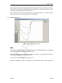
1
DR
AF
MWell
T
Design and design check for multi layer well systems
DR
AF
T
T
DR
AF
MWell
Design and design check for multi layer well systems
User Manual
Version: 15.1
Revision: 41593
24 September 2015
DR
AF
T
MWell, User Manual
Published and printed by:
Deltares
Boussinesqweg 1
2629 HV Delft
P.O. 177
2600 MH Delft
The Netherlands
For sales contact:
telephone: +31 88 335 81 88
fax:
+31 88 335 81 11
e-mail:
[email protected]
www:
http://www.deltaressystems.nl
telephone:
fax:
e-mail:
www:
+31 88 335 82 73
+31 88 335 85 82
[email protected]
https://www.deltares.nl
For support contact:
telephone: +31 88 335 81 00
fax:
+31 88 335 81 11
e-mail:
[email protected]
www:
http://www.deltaressystems.nl
Copyright © 2015 Deltares
All rights reserved. No part of this document may be reproduced in any form by print, photo
print, photo copy, microfilm or any other means, without written permission from the publisher:
Deltares.
Contents
1 General Information
1.1 Preface . . . . . . . . . . . . .
1.2 Features in standard module . .
1.3 History . . . . . . . . . . . . .
1.4 Assumptions and Limitations . .
1.5 Minimum System Requirements
1.6 Definitions and Symbols . . . .
1.7 Getting Help . . . . . . . . . .
1.8 Getting Support . . . . . . . . .
1.9 Deltares . . . . . . . . . . . .
1.10 Deltares Systems . . . . . . . .
.
.
.
.
.
.
.
.
.
.
.
.
.
.
.
.
.
.
.
.
.
.
.
.
.
.
.
.
.
.
.
.
.
.
.
.
.
.
.
.
.
.
.
.
.
.
.
.
.
.
.
.
.
.
.
.
.
.
.
.
.
.
.
.
.
.
.
.
.
.
.
.
.
.
.
.
.
.
.
.
1
1
1
2
2
3
3
4
4
6
6
.
.
.
.
.
.
.
.
.
.
.
.
.
.
.
.
.
.
.
.
.
.
.
.
.
.
.
.
.
.
.
.
.
.
.
.
.
.
.
.
.
.
.
.
.
7
7
7
8
9
9
11
12
12
12
.
.
.
.
.
.
.
.
.
.
.
.
.
.
.
.
.
.
.
.
15
15
15
15
18
.
.
.
.
.
.
.
.
.
.
.
.
19
19
19
19
20
23
23
23
24
25
26
27
27
.
.
.
.
.
.
.
29
29
29
29
30
31
32
32
.
.
.
.
.
.
.
.
.
.
.
.
.
.
.
.
.
.
.
.
.
.
.
.
.
.
.
.
.
.
.
.
.
.
.
.
.
.
.
.
.
.
.
.
.
.
.
.
.
.
.
.
.
.
.
.
.
.
.
.
.
.
.
.
.
.
.
.
.
.
.
.
.
.
.
.
.
.
.
.
.
.
.
.
.
.
.
.
.
.
2 Getting Started
2.1 Starting MWell . . . . . . . . . . . . . . . . . . . .
2.2 Main Window . . . . . . . . . . . . . . . . . . . . .
2.2.1 Menu bar . . . . . . . . . . . . . . . . . . .
2.2.2 Icon bar . . . . . . . . . . . . . . . . . . .
2.2.3 Input Diagram window . . . . . . . . . . . .
2.2.4 Stratification window (profile with soil clusters)
2.2.5 Info bar . . . . . . . . . . . . . . . . . . . .
2.2.6 Status bar . . . . . . . . . . . . . . . . . .
2.3 Files . . . . . . . . . . . . . . . . . . . . . . . . .
.
.
.
.
.
.
.
.
.
.
.
.
.
.
.
.
.
.
.
.
.
.
.
.
.
.
.
.
.
.
.
.
.
.
.
.
.
.
.
.
.
.
.
.
.
.
.
.
.
.
.
.
.
.
.
.
.
.
.
.
.
.
.
3 General
3.1 File menu . . . . . . . .
3.2 Tools menu . . . . . . .
3.2.1 Program Options
3.3 Help menu . . . . . . .
.
.
.
.
.
.
.
.
.
.
.
.
.
.
.
.
.
.
.
.
.
.
.
.
.
.
.
.
DR
AF
.
.
.
.
.
.
.
.
.
.
T
Contents
.
.
.
.
4 Input
4.1 Project menu . . . . . . .
4.1.1 Model . . . . . .
4.1.2 Location Map . . .
4.1.3 Project Properties
4.1.4 View Input File . .
4.2 Geometry menu . . . . .
4.2.1 Profile . . . . . .
4.2.2 Discharge Wells .
4.2.3 Sheet Pilings . . .
4.2.4 Mesh . . . . . . .
4.3 Water menu . . . . . . . .
4.3.1 Water Properties .
5 Calculations
5.1 Calculation input . . . .
5.1.1 Monitoring Points
5.1.2 Contouring Times
5.1.3 Monitoring Times
5.2 Start Calculation . . . .
5.3 Warning . . . . . . . .
5.4 Error Messages . . . . .
6 View Results
Deltares
.
.
.
.
.
.
.
.
.
.
.
.
.
.
.
.
.
.
.
.
.
.
.
.
.
.
.
.
.
.
.
.
.
.
.
.
.
.
.
.
.
.
.
.
.
.
.
.
.
.
.
.
.
.
.
.
.
.
.
.
.
.
.
.
.
.
.
.
.
.
.
.
.
.
.
.
.
.
.
.
.
.
.
.
.
.
.
.
.
.
.
.
.
.
.
.
.
.
.
.
.
.
.
.
.
.
.
.
.
.
.
.
.
.
.
.
.
.
.
.
.
.
.
.
.
.
.
.
.
.
.
.
.
.
.
.
.
.
.
.
.
.
.
.
.
.
.
.
.
.
.
.
.
.
.
.
.
.
.
.
.
.
.
.
.
.
.
.
.
.
.
.
.
.
.
.
.
.
.
.
.
.
.
.
.
.
.
.
.
.
.
.
.
.
.
.
.
.
.
.
.
.
.
.
.
.
.
.
.
.
.
.
.
.
.
.
.
.
.
.
.
.
.
.
.
.
.
.
.
.
.
.
.
.
.
.
.
.
.
.
.
.
.
.
.
.
.
.
.
.
.
.
.
.
.
.
.
.
.
.
.
.
.
.
.
.
.
.
.
.
.
.
.
.
.
.
.
.
.
.
.
.
.
.
.
.
.
.
.
.
.
.
.
.
.
.
.
.
.
.
.
.
.
.
.
.
.
.
.
.
.
.
.
.
.
.
.
.
.
.
.
.
.
.
.
.
.
.
.
.
.
.
.
.
.
.
.
.
.
.
.
.
.
.
.
.
.
.
.
.
.
.
.
.
.
.
.
.
.
.
.
.
.
.
.
.
.
.
.
.
.
.
.
.
.
.
.
.
.
.
.
.
.
.
.
.
.
.
.
.
.
.
.
.
.
.
.
.
.
.
.
.
.
.
.
.
.
.
.
.
.
.
.
.
.
.
.
.
.
.
.
.
.
.
.
.
.
.
.
.
.
.
.
.
.
.
.
.
.
.
.
.
.
.
.
.
.
.
.
.
.
.
.
.
.
.
.
.
.
.
.
.
.
.
.
.
.
.
.
.
.
.
.
.
.
.
.
.
.
.
.
.
.
.
.
.
.
.
.
.
.
.
.
.
.
.
.
.
.
.
.
.
.
.
.
.
.
.
.
.
.
.
.
.
.
.
.
.
.
.
.
.
.
.
.
.
.
.
.
.
.
.
.
.
.
.
.
.
.
.
.
.
.
.
.
.
.
.
.
.
.
.
.
.
.
.
.
.
.
.
.
.
.
.
.
.
.
.
.
.
.
.
.
.
.
.
.
.
.
.
.
.
.
.
.
.
.
.
33
iii
MWell, User Manual
6.1
6.2
6.3
Report . . . . . . . . . . . . . . . . . . . . . . . . . . . . . . . . . . . . 33
Contour Plot . . . . . . . . . . . . . . . . . . . . . . . . . . . . . . . . . 35
Time History Chart . . . . . . . . . . . . . . . . . . . . . . . . . . . . . . 37
.
.
.
.
.
.
.
.
.
.
.
.
.
.
.
.
.
.
.
.
.
.
.
.
.
.
.
.
.
.
.
.
.
.
.
.
.
.
.
.
.
.
.
.
.
.
.
.
39
39
40
40
40
41
42
43
44
44
45
46
46
49
DR
AF
Bibliography
.
.
.
.
.
.
.
.
.
.
.
.
T
7 Theory of groundwater flow
7.1 Basic Equations . . . . . . . . . . . . . . . . . . . . . . . . . .
7.2 Solution Method . . . . . . . . . . . . . . . . . . . . . . . . . .
7.3 Groundwater flow and sheet pilings . . . . . . . . . . . . . . . . .
7.3.1 Background . . . . . . . . . . . . . . . . . . . . . . . .
7.3.2 Accuracy of the calculations . . . . . . . . . . . . . . . .
7.3.3 Use of sheet pilings in MWell . . . . . . . . . . . . . . . .
7.3.4 Example of the effect of sheet pilings from the Results menu
7.4 Hydro-geological parameter values . . . . . . . . . . . . . . . . .
7.5 Permeability, Transmissivity and Resistance . . . . . . . . . . . . .
7.6 Sheet piling flow resistance . . . . . . . . . . . . . . . . . . . . .
7.7 Specific storage coefficient . . . . . . . . . . . . . . . . . . . . .
7.8 Oedometer stiffness . . . . . . . . . . . . . . . . . . . . . . . .
iv
Deltares
List of Figures
List of Figures
1.1
1.2
1.3
1.4
MWell contouring plot . . . . . . . . . . . . . . . . . . . . . . . .
‘Software’ menu of the Deltares Systems website (www.deltares.com)
Support window, Problem Description tab . . . . . . . . . . . . . .
Send Support E-Mail window . . . . . . . . . . . . . . . . . . . .
.
.
.
.
.
.
.
.
.
.
.
.
.
.
.
.
.
.
.
.
2.1
2.2
2.3
2.4
2.5
2.6
Modules window . . .
MWell main window . .
MWell menu bar . . .
MWell icon bar . . . .
Input Diagram window
Stratification window .
3.1
3.2
3.3
3.4
Program Options
Program Options
Program Options
Program Options
.
.
.
.
.
.
.
.
.
.
.
.
.
.
.
.
.
.
.
.
.
.
.
.
.
.
.
.
.
.
.
.
.
.
.
.
.
.
.
.
.
.
.
.
.
.
.
.
.
.
.
.
.
.
.
.
.
.
.
.
.
.
.
.
.
.
.
.
.
.
.
.
.
.
.
.
.
.
.
.
.
.
.
.
.
.
.
.
.
.
.
.
.
.
.
.
.
.
.
.
.
.
.
.
.
.
.
.
.
.
.
.
.
.
.
.
.
.
.
.
.
.
.
.
.
.
.
.
.
.
.
.
.
.
.
.
.
.
.
.
.
.
.
.
.
.
.
.
.
.
.
.
.
.
.
.
. 7
. 8
. 8
. 9
. 10
. 11
window, View tab . .
window, General tab
window, Locations tab
window, Modules tab
.
.
.
.
.
.
.
.
.
.
.
.
.
.
.
.
.
.
.
.
.
.
.
.
.
.
.
.
.
.
.
.
.
.
.
.
.
.
.
.
.
.
.
.
.
.
.
.
.
.
.
.
.
.
.
.
.
.
.
.
.
.
.
.
.
.
.
.
.
.
.
.
.
.
.
.
.
.
.
.
16
16
17
17
Model window . . . . . . . . . . . . . . . . . . . . . . . . . . .
Location Map window . . . . . . . . . . . . . . . . . . . . . . . .
Project Properties window, Identification tab . . . . . . . . . . . .
Project Properties window, Input View tab . . . . . . . . . . . . .
Project Properties window, Contour Plot Settings tab . . . . . . . .
Profile window . . . . . . . . . . . . . . . . . . . . . . . . . . .
Discharge Wells window . . . . . . . . . . . . . . . . . . . . . .
Sheet Pilings window . . . . . . . . . . . . . . . . . . . . . . . .
Input Diagram window showing the sheet pilings, the discharge wells
monitoring points . . . . . . . . . . . . . . . . . . . . . . . . . .
4.10 Mesh window . . . . . . . . . . . . . . . . . . . . . . . . . . . .
4.11 Water Properties window . . . . . . . . . . . . . . . . . . . . . .
. . . .
. . . .
. . . .
. . . .
. . . .
. . . .
. . . .
. . . .
and the
. . . .
. . . .
. . . .
.
.
.
.
.
.
.
.
19
20
20
21
22
23
24
25
5.1
5.2
5.3
5.4
Monitoring Points window .
Contouring Times window
Monitoring Times window .
Start Calculation window .
.
.
.
.
.
.
.
.
.
.
.
.
.
.
.
.
.
.
.
.
.
.
.
.
.
.
.
.
.
.
.
.
.
.
.
.
.
.
.
.
.
.
.
.
.
.
.
.
.
.
.
.
.
.
.
.
.
.
.
.
.
.
.
.
.
.
.
.
.
.
.
.
.
.
.
.
.
.
.
.
.
.
.
.
.
.
.
.
.
.
.
.
29
30
30
31
6.1
6.2
6.3
6.4
Report window (short report) . . .
Contour Plot window for Drawdown
Contour Plot window for Settlement
Time History Chart window . . . .
.
.
.
.
.
.
.
.
.
.
.
.
.
.
.
.
.
.
.
.
.
.
.
.
.
.
.
.
.
.
.
.
.
.
.
.
.
.
.
.
.
.
.
.
.
.
.
.
.
.
.
.
.
.
.
.
.
.
.
.
.
.
.
.
.
.
.
.
.
.
.
.
.
.
.
.
.
.
.
.
.
.
.
.
.
.
.
.
34
35
36
37
7.1
7.2
7.3
Start Calculation window . . . . . . . . . . . . . . . . . . . . . . . . . . . 41
Time History Chart window . . . . . . . . . . . . . . . . . . . . . . . . . . 42
Contour Plot window . . . . . . . . . . . . . . . . . . . . . . . . . . . . . 43
DR
AF
4.1
4.2
4.3
4.4
4.5
4.6
4.7
4.8
4.9
T
.
.
.
.
.
.
2
5
5
6
Deltares
.
.
.
.
.
.
.
.
.
.
.
.
. 26
. 27
. 27
v
DR
AF
T
MWell, User Manual
vi
Deltares
List of Tables
List of Tables
5.3
Limits input in MWell . . . . . . . . . . . . . . . . . . . . . . . . . . . . . 32
7.1
7.2
Typical values of the hydraulic conductivity for different soil types . . . . . . . 45
Average values for the reciprocal hydraulic joint resistance followed from tests
performed for Arcelor . . . . . . . . . . . . . . . . . . . . . . . . . . . . . 45
Typical values of porosity for different soil types . . . . . . . . . . . . . . . . 46
DR
AF
T
7.3
Deltares
vii
DR
AF
T
MWell, User Manual
viii
Deltares
1 General Information
1.1
Preface
MWell is a tool to facilitate fast and flexible calculations of the drawdown and settlement due
to well pumping in a set of permeable aquifers and less permeable aquitards. The settlement
calculation also involves the compression of the aquitards.
The MWell program determines the transient flow field in a multilayered drainage system. The
layers consist of intermittent aquifers and aquitards. In the permeable aquifers wells may be
placed to pump up water, which flows mainly horizontally to the filters. The semi-permeable
aquitards cause the water to leak in-between the aquifers in a more or less vertical fashion.
An elegant and powerful method is available to determine the flow in the layered geometry:
T
the technique of matrix diagonalisation.
all layers have a constant thickness and extend indefinitely
every separate layer is homogeneous
the flow in the aquifers is mainly horizontal, determined by transmissivity and storage.
the flow in the aquitards is mainly vertical, controlled by resistance and storage.
every well has a filter over the complete height of one aquifer.
DR
AF
The inverse Laplace Transformation of the solution is performed by an approach according to
Stehfest.
Features in standard module
MWell determines the transient flow and settlement by pumping with fully penetrating wells,
in a set of horizontal permeable aquifers and less permeable aquitards. MWell gives quick
solutions and is easy to use. The following features are included:
multi-layer geometry
transient flow process
several pumping units per layer
Two types of graphical output:
1.2
time history plot
contouring plots in SURFER format
An example of a contouring plot is presented in the figure below. The geometry consists of
three sand layers. In the middle one four pumps are placed. In the bottom one four pumps
too. The interaction between the layers is clearly visible.
Deltares
1 of 49
DR
AF
T
MWell, User Manual
Figure 1.1: MWell contouring plot
1.3
History
The first version of MWell was built by GeoDelft in 1997, based on the mathematical method
developed by Maas (1983).
Release 2.7 (2003) uses a new licensing method. The storativity parameter has been
replaced by the oedometer stiffness. The deformation contribution of aquifers is now
included in the total settlement.
Release 2.8 (2004) has some corrections in the user interface. Plots have been improved by added a title header with relevant information. The Help file was updated.
Release 3.1 (2008) facilitates also to calculate the effect of the presence of low permeable walls (fully penetrating in an aquifer) on groundwater flow.
Release 3.3 (2011) improves the implementation of Stehfest for projects with sheet
piling defined.
Release 14.1 (2014) includes minor fixes in the user interface and a new license system.
1.4
Assumptions and Limitations
The program calculates drawdown with respect to an initial groundwater level with a
zero setting;
All layers have a constant thickness and extend to infinity;
Every separate layer is homogeneous and completely saturated;
The flow in the permeable aquifers is only horizontal, the flow in the less permeable
aquitards is only vertical;
2 of 49
Deltares
General Information
Each well has a filter over the complete height of one aquifer;
Each flow resisting wall (from now on referred to as Sheet Piling) is present over the
complete height of one aquifer;
Horizontal deformations are assumed to be zero;
Only the influence of drawdown on settlements is considered, the influence of dead
weight and soil loads is neglected.
T
The analytical calculation method has in principle no limitations. However, numerical accuracy
of the computer may interfere with the performance. Two types of numerical instability may
occur:
Singular behavior of the value matrices due to large contrasts in the soil parameters in
a many-layered system.
Divergent behavior in the Stehfest inverse placeLaplace transformation; this rarely hap-
1.5
DR
AF
pens close after the start of pumping.
Minimum System Requirements
The following minimum system requirements are needed in order to run and install the MWell
software, either from CD or by downloading from the Deltares website via MS Internet Explorer:
Operating systems:
Windows 2003,
Windows Vista,
Windows 7 – 32 bits
Windows 7 – 64 bits
Windows 8
Hardware specifications:
1 GHz Intel Pentium processor or equivalent
512 MB of RAM
400 MB free hard disk space
SVGA video card, 1024 × 768 pixels, High colors (16 bits)
CD-ROM drive
Microsoft Internet Explorer version 6.0 or newer (download from www.microsoft.com)
1.6
Definitions and Symbols
Soil:
σz0
εz
φ
S
t
D
D0
k
k0
Deltares
kN/m2
m
m
d
m
m
m/d
m/d
Vertical effective stress (positive in compression)
Vertical strain (positive in compression)
Hydraulic head by flow and deformation
Variation of water storage (i.e. drawdown)
Time
Thickness of an aquifer
Thickness of a semi-impervious layer (i.e. aquitard)
Horizontal hydraulic conductivity of an aquifer
Vertical hydraulic conductivity of a semi-impervious layer (i.e.
aquitard)
3 of 49
MWell, User Manual
c
d
Vertical hydraulic resistance of a semi-impervious layer (i.e.
aquitard):
c = D0 /k 0
kD
n
Eoed
G
cV
KD
khead
m /d
kN/m2
kN/m2
m2 /d
kN/m2
m/d
Sheet Piling:
ρ
m/d
R
d
b
m
Transmissivity of an aquifer
Porosity
Oedometer stiffness
Shear modulus
Consolidation coefficient
Bulk modulus of the drained soil skeleton
Darcy permeability
Reciprocal hydraulic joint resistance
Sheet piling flow resistance
Sheet piling width
Pore fluid:
[kN/m2 ]
[kN/m3 ]
1.7
Bulk modulus of the pore fluid
Unit weight of the pore fluid
DR
AF
Kf
γf
T
2
Getting Help
From the Help menu, choose the Manual option to open the User Manual of MWell in PDF
format. Here help on a specific topic can be found by entering a specific word in the Find field
of the PDF reader.
1.8
Getting Support
Deltares Systems tools are supported by Deltares. A group of 70 people in software development ensures continuous research and development. Support is provided by the developers
and if necessary by the appropriate Deltares experts. These experts can provide consultancy
backup as well.
If problems are encountered, the first step should be to consult the online Support at:
www.deltares.com in menu ‘Software’. Different information about the program can be found
on the left-hand side of the window (Figure 1.2):
In ‘Support - Frequentely asked questions’ are listed the most frequently asked technical
questions and their answers.
In ‘Support - Known issues’ are listed the issues of the program.
In ‘Release notes D-Geo Pipeline’ are listed the differences between an old and a new
version.
4 of 49
Deltares
General Information
T
Figure 1.2: ‘Software’ menu of the Deltares Systems website (www.deltares.com)
DR
AF
If the solution cannot be found there, then the problem description can be e-mailed (preferred)
or faxed to the Deltares Systems support team. When sending a problem description, please
add a full description of the working environment. To do this conveniently:
Open the program.
If possible, open a project that can illustrate the question.
Choose the Support option in the Help menu. The System Info tab contains all relevant
information about the system and the DSeries software. The Problem Description tab
enables a description of the problem encountered to be added.
Figure 1.3: Support window, Problem Description tab
After clicking on the Send button, the Send Support E-Mail window opens, allowing
sending current file as an attachment. Marked or not the Attach current file to mail
checkbox and click OK to send it.
Deltares
5 of 49
MWell, User Manual
Figure 1.4: Send Support E-Mail window
1.9
Deltares
T
The problem report can either be saved to a file or sent to a printer or PC fax. The document
can be emailed to [email protected] or alternatively faxed to +31(0)88 335
8111.
DR
AF
Since January 1st 2008, GeoDelft GeoDelft together with parts of Rijkswaterstaat /DWW,
RIKZ and RIZA, WL |Delft Hydraulics and a part of TNO Built Environment and Geosciences
are forming the Deltares Institute, a new and independent institute for applied research and
specialist advice. Founded in 1934, GeoDelft was one of the world’s most renowned institutes for geotechnical and environmental research. As a Dutch national Grand Technological
Institute (GTI), Deltares role is to obtain, generate and disseminate geotechnical know-how.
The institute is an international leader in research and consultancy into the behavior of soft
soils (sand clay and peat) and management of the geo-ecological consequences which arise
from these activities. Again and again subsoil related uncertainties and risks appear to be
the key factors in civil engineering risk management. Having the processes to manage these
uncertainties makes Deltares the obvious Partner in risk management for all parties involved
in the civil and environmental construction sector. Deltares teams are continually working on
new mechanisms, applications and concepts to facilitate the risk management process, the
most recent of which is the launch of the concept "GeoQ" into the geotechnical sector.
For more information on Deltares, visit the Deltares website: www.deltares.nl.
1.10
Deltares Systems
Deltares Systems (formerly known as Delft GeoSystems) was founded in 2002. The company’s objective is to convert Deltares knowledge into practical geo-engineering services and
software. Deltares Systems has developed a suite of software for geotechnical engineering.
Besides software, Deltares Systems is involved in providing services such as hosting on-line
monitoring platforms, hosting on-line delivery of site investigation, laboratory test results, etc.
As part of this process Deltares Systems is progressively connecting these services to their
software. This allows for more standardized use of information, and the interpretation and
comparison of results. Most software is used as design software, following design standards.
This however, does not guarantee a design that can be executed successfully in practice, so
automated back-analyses using monitoring information are an important aspect in improving
geotechnical engineering results. For more information about Deltares Systems’ geotechnical
software, including download options, visit www.deltaressystems.com
6 of 49
Deltares
2 Getting Started
This Getting Started chapter aims to familiarize the user with the structure and user interface
of MWell. The Tutorial section which follows uses a selection of case studies to introduce the
program’s functions. Getting Started
2.1
Starting MWell
DR
AF
T
To start MWell, click Start on the Windows menu bar and then find it under Programs, or
double-click a MWell input file that was generated during a previous session. For an MWell
installation based on floating licenses, the ModulesModules window may appear at startup
Figure 2.1. Check that the correct modules are selected and click OK.
Figure 2.1: Modules window
When MWell is started from the Windows menu bar, the last project that was worked on will
open automatically, unless the program has been configured otherwise under Tools: Program
Options.
2.2
Main Window
When MWell is started, the main window is displayed Figure 2.2. This window contains a
menu bar section 2.2.1, an icon bar section 2.2.2, an Input Diagram window section 2.2.3
that displays the pre-selected or most recently accessed project, the Stratification window
section 2.2.4, an info bar section 2.2.5 and a status bar section 2.2.6.
The Input Diagram window displays a top view layout of the wells and the Stratification window
shows a vertical cross section of the stratification. In case of a new file both windows are
empty.
Deltares
7 of 49
DR
AF
T
MWell, User Manual
Figure 2.2: MWell main window
2.2.1
Menu bar
To access the MWell menus, click the menu names on the menu bar.
Figure 2.3: MWell menu bar
The menus contain the following functions:
File
Standard Windows options for opening and saving files as well as several
MWell options for exporting and printing active windows and reports.
Project
Options for defining or not sheet piling, defining properties and viewing the
input file section 4.1.
Geometry Options for adding or editing soil profile (i.e. clusters of aquitards and
aquifers), wells (position and discharge), sheet pile walls, the top view area
and mesh for contouring section 4.2.
Water
Input of water parameters section 4.3.
Calculation Options for editing the points and time grid for time history chart and analysis
of the drawdown and settlements, based on input values chapter 5.
Results
Options for creating report and displaying the drawdown and settlements using contour plots or time-history charts chapter 6.
Tools
Options for editing MWell program defaults section 3.2.
Window
Default Windows options for arranging the MWell windows and choosing the
active window.
Help
Online Help options section 1.7.
Detailed descriptions of these menu options can be found in the Reference section.
8 of 49
Deltares
Getting Started
2.2.2
Icon bar
Use the buttons on the icon bar to quickly access frequently used functions (see below).
Buttons on icon barIcon bar
Figure 2.4: MWell icon bar
Click on the following buttons to activate the corresponding functions:
Start a new MWell project.
T
Open the input file of an existing project.
Save the input file of the current project.
Print the contents of the currently active window.
DR
AF
Display a print preview of the current contents of the Input Diagram window.
Open the Project Properties window. Here the project title and other identification data can be entered, and the Diagram Settings and Graph Settings for
the project can be determined.
Start the main calculation.
Display the contents of online Help.
Display the first page of the Delft GeoSystems website:
www.delftgeosystems.nl
2.2.3
Input Diagram window
The Input Diagram window graphically displays the input in two separate sub-windows:
a top view layout of the wells;
a vertical cross section of the stratification.
In case of a new file both sub-windows are empty. Editing wells is performed by the technique
of selecting, dragging and double clicking on the corresponding item or by using the Edit
panel.
Deltares
9 of 49
DR
AF
T
MWell, User Manual
Figure 2.5: Input Diagram window
Click on the buttons in the Edit or Tools panel to activate the corresponding functions:
Select and Edit
In this mode, the left-hand mouse button can be used to select previously defined
supports, loads and layers in the Input Diagram. Items can then be deleted or
modified by dragging or resizing, or by clicking the right hand mouse button and
choosing an option from the menu displayed. Pressing the Escape key will return
the user to this Select and Edit mode.
Pan
Click this button to move the drawing by clicking and dragging the mouse.
Zoom in
Click this button to enlarge the drawing, and then click on the drawing on the part
which is to be at the centre of the new image.
Zoom out
Click this button, and then click on the drawing, to reduce the drawing.
Zoom area
Click this button then click and drag a rectangle over the area to be enlarged. The
selected area will be enlarged to fit the window.
Measure the distance between two points
Click this button, then click the first point on the Input Diagram window and place
the cross on the second point. The distance between the two points can be read at
the bottom of the Input View window. To turn this option off, click the escape key.
Add Well
Click this button to add wells.
Add Monitoring Place
Click this button to add monitoring points.
Undo Zoom
Click this button to undo the zoom.
Zoom limits
Click this button to display the complete drawing.
10 of 49
Deltares
Getting Started
Mesh On/Off
Click this button to view or not the mesh.
For more information, see section 4.2.
Stratification window (profile with soil clusters)
T
The stratification window at the right of the main window displays the soil profile soil consisting
of a number of soil clusters Figure 2.6. A cluster is a semi-pervious (low permeability) layer
(aquitard) on top of a permeable layer (aquifer). The flow in the aquitard is mainly vertical,
while the flow in the aquifer is mainly horizontal. The layers have a constant thickness and
extend to infinity.
Clusters are numbered. The number is shown in the stratification window. The individual
aquitards and aquifers can be named too. To distinguish the layers a color may be chosen
from a pre-selected set. The required data are entered via edit boxes.
The bottom of the geometry is assumed to be impervious.
DR
AF
2.2.4
Figure 2.6: Stratification window
Profile properties
Click this button to open the Profile window section 4.2.1 and edit/modify the
soil profile.
Zoom in
Click this button to enlarge the drawing, and then click on the drawing on the
part which is to be at the centre of the new image.
Zoom out
Click this button, and then click on the drawing, to reduce the drawing.
Zoom limits
Click this button to display the complete drawing.
Deltares
11 of 49
MWell, User Manual
Print
Click this button to print the soil stratification.
2.2.5
Info bar
This bar situated at the bottom of the Input Diagram window displays the co-ordinates of the
current position of the cursor and the distance between two points when the icon Measure the
distance between two points is selected from the Edit panel.
2.2.6
Status bar
T
All programs by Delft GeoSystems like MWell take the Y-coordinate for the vertical direction.
As a result the position in the horizontal plane is defined by the X and Z co-ordinates.
2.3
Files
*.wec
*.wed
*.wedx
*.weh
*.wei
*.weo
*.wes
12 of 49
DR
AF
This bar situated at the bottom of the main window displays a description of the selected icon
of the icon bar section 2.2.2 or of the Input Diagram window section 2.2.3.
Mesh file (ASCII): Contains the mesh data.
Dump file (ASCII): Contains calculation results used in the short report section 6.1.
Dump file (ASCII): Contains calculation results used in the long report section 6.1.
Dump file (ASCII): Used to visualize the drawdown and settlements in the
Time History Chart window of the Results menu section 6.3.
Input file (ASCII): Contains the input with the problem definition. After interactive generation, this file can be re-used in subsequent MWell analyses.
Output file (ASCII): After a calculation has been performed, all output is written to this file.
Setting file (ASCII):
Working file with settings data. This file doesn’t contain any information that is
relevant for the calculation, but only settings that apply to the representation
of the data, such as the grid size.
Deltares
Tutorial
DR
AF
T
No tutorial available yet. As example files, open one of the demo files in the installation
directory of MWell.
Deltares
13 of 49
DR
AF
T
MWell, User Manual
14 of 49
Deltares
3 General
This chapter contains a detailed description of the available menu options for inputting data
for a project, and for calculating and viewing the results. The examples in the tutorial section
provide a convenient starting point for familiarization with the program.
3.1
File menu
Besides the familiar Windows options for opening and saving files, the File menu contains a
number of options specific to MWell:
Copy Active Window to Clipboard
Export Active Window
T
Use this option to copy the contents of the active window to the Windows clipboard so
that they can be pasted into another application. The contents will be pasted in either
text format or Windows Meta File format.
DR
AF
Use this option to export the contents of the active window as a Windows Meta File
(*.wmf), a Drawing Exchange File (*.dxf) or a text file (*.txt).
Export Report
This option allows the report to be exported in a different format, such as pdf or rtf.
Page Setup
This option allows definition of the way MWell plots and reports are to be printed. The
printer, paper size, orientation and margins can be defined as well as whether and
where axes are required for plots. Click Autofit to get MWell to choose the best fit for
the page.
Print Preview Active Window
This option will display a print preview of the current contents of the Input Diagram or
Results window.
Print Active Window
This option printsthe current contents of the Input Diagram or Results window.
Print Preview Report
This option will display a print preview of the calculation report.
Print Report
This option printsthe calculation report.
3.2
3.2.1
Tools menu
Program Options
On the menu bar, click Tools and then choose Options to open the corresponding input window. In this window, the user can optionally define their own preferences for some of the
program’s default values.
Deltares
15 of 49
MWell, User Manual
T
View
Figure 3.1: Program Options window, View tab
General
Mark the relevant checkbox to display the tool bar and/or status bar each time
MWell is started.
Mark this checkbox to display the project titles, as entered on the Identification
tab, in a panel at the bottom of the Input Diagram window.
DR
AF
Toolbar
Status bar
Title panel
Figure 3.2: Program Options window, General tab
Startup
with
Save on
Calculation
16 of 49
Click one of these toggle buttons to determine how a project should be initiated each time MWell is started.
No project: Use the buttons in the toolbar or the options in the File menu to
open an existing project or to start a new one.
Last used project: The last project to be worked on is opened automatically.
New project: A new project is created comprising a sheet pile wall with a
"dummy" soil layer on both sides.
NOTE: The Startup with option is ignored when MWell is started by doubleclicking on an input file.
The toggle buttons determine how input data is saved prior to calculation. It
can either be saved automatically, using the same file name each time, or a
file name can be specified every time the data is saved.
Deltares
General
Use Enter
key to
Use the toggle buttons to determine the way the Enter key is used in MWell:
either as an equivalent of pressing the default button (Windows style) or to
shift the focus to the next item in a window (for users accustomed to the DOS
version(s) of the program).
DR
AF
T
Locations
Figure 3.3: Program Options window, Locations tab
Working
directory
MWell will start up with a working directory for selection and saving of files.
Either choose to use the last used directory, or specify a fixed path.
Modules
Figure 3.4: Program Options window, Modules tab
For a MWell installation based on floating licenses, the Modules tab can be used to claim a
license for the particular modules that are to be used. If the Show at start of program checkbox
is marked then this window will always be shown at start-up.
For a MWell installation based on a license dongle, the Modules tab will just show the modules
that may be used.
Deltares
17 of 49
MWell, User Manual
Help menu
The Help menu allows access to:
Get on-line help using the MWell Help option (refer to section 1.7 for a detailed description of this window);
View Error Messages;
View the Manual;
Visit the Deltares Systems Website for the latest news;
Use the Support option to register program errors (refer to section 1.8 for a detailed
description of this window);
Display the About-box of MWell (About MWell).
T
DR
AF
3.3
18 of 49
Deltares
4 Input
MWell facilitates calculation of pumping in multi-layered subsoil. The filters are placed in
aquifers, which are separated by aquitards. The flow can be manipulated by placing semiimpermeable walls (sheet pilings). The drawdown and the settlements in all aquifers are
determined.
Material data consist of height, transmissivity, oedometer stiffness and porosity for the aquifers
and height, resistance, oedometer stiffness and porosity for the aquitards. The height of the
individual layers is shown in the vertical cross section of the stratification.
All programs by Delft GeoSystems like MWell take the Y-coordinate for the vertical direction.
As a result the position in the horizontal plane is defined by the X and Z co-ordinates.
T
The wells require a discharge (positive value for pumping) or a recharge (negative value for
infiltration), a filter position and a time switch on and off. Moreover the X, Z position is specified
and the effective radius of the well. The latter is intended to include a gravel casing, if any is
present in the borehole for a well.
4.1
DR
AF
Before analysis can be started, data’s for the sheet pile wall, soil, loads and supports need to
be inputted.
Project menu
Each project starts with the selection of an analysis model and the entry of general details
about the project.
4.1.1
Model
On the menu bar, click Project and then choose Model to open the input window. In this
window the Sheet piling option can be selected.
Figure 4.1: Model window
4.1.2
Location Map
An important feature of MWell is the possibility to import a background picture. This picture
can be used for orientation when defining the positions of wells, monitoring points and sheet
pilings.
The background picture may be of different formats (jpg, jpeg, bmp, emf, wmf). The limits of
the picture must be specified in the coordinate system chosen for the definition of the project.
Deltares
19 of 49
MWell, User Manual
Figure 4.2: Location Map window
4.1.3
DR
AF
Copy co-ordinates to
mesh on pressing OK
The location of the file to import.
The position in the geometry by the limits in the X, Z coordinate
plane of Left X, Right X, Top Z, Bottom Z [m].
If desired, it is possible to take the picture limits also as the limits
of the calculation mesh by checking this option in the dialog box.
T
Background Picture
Co-ordinates
Project Properties
On the menu bar, click Project and then choose Properties to open the input window. The
Project Properties window contains several tabs, which allow the settings for the current
project to be changed.
Project Properties – Identification
Use the Identification tab to specify the project identification data. Identification
Figure 4.3: Project Properties window, Identification tab
Titles
20 of 49
Use Title 1 to give the project a unique, easily recognizable
name. Title 2 and Title 3 can be added to indicate specific characteristics of the calculation. The three titles will be included on
printed output.
Deltares
Input
Date
The date entered here will be used on printouts and graphic plots
for this project. Either mark the Use current date checkbox to
automatically use the current date on each printout, or enter a
specific date.
Enter the name of the user performing the calculation or generating the printout.
Enter a project identification number.
Specify the annex number of the printout.
Drawn by
Project ID
Annex ID
Project Properties – Input View
T
Mark the checkbox Save as default to use these settings every time MWell is started or a new
project is created.
DR
AF
Use the Input View tab to specify the lay-out of the input view.
Figure 4.4: Project Properties window, Input View tab
Rulers
Info bar
Same scale for X and Z
axis
Show grid
Snap to Grid
Grid distance
Wells
Monitoring points
Deltares
Mark this checkbox to display the horizontal and vertical rulers.
Mark this checkbox to display the information bar at the bottom
of the Input Diagram window.
Mark this checkbox to use the same scale for the horizontal and
vertical directions.
Mark this checkbox to display a grid in each Input Diagram window.
Mark this checkbox to ensure that objects align to the grid automatically when they are moved or positioned in a drawing window. This option applies only to graphical input.
Use this field to set the distance between grid points.
Mark this checkbox to display Wells in the Input Diagram window.
This option is available only for a sheet pile wall or a pile loaded
by forces.
Mark this checkbox to display monitoring points in the Input Diagram window.
21 of 49
MWell, User Manual
Labels
Mark this checkbox to display labels in the Input Diagram window.
Project Properties – Contour Plot Settings
DR
AF
T
Use the Contour Plot Settings tab to specify the display of the Contour Plot window.
Figure 4.5: Project Properties window, Contour Plot Settings tab
Info bar
Legend
Options panel
Same scale for X and Z
axis
Rulers
Mesh
Show values in plot
Contour options
Contour range
22 of 49
Mark this checkbox to display the information bar at the bottom
of the Contour Plot window.
Mark this checkbox to display the legend.
Mark this checkbox to display the options panel.
Mark this checkbox to use the same scale for the horizontal and
vertical directions.
Mark this checkbox to display the horizontal and vertical rulers.
Mark this checkbox to display the mesh.
Mark this checkbox to display values labels. When using this
option the distance between the value labels for the contouring
must be entered.
The contour options concern the presentation of colored areas
(shades) and/or lines. For the presentation of colors a palette
must be chosen. This palette is also used for the presentation in
the legend.
The contour range defines the number of color areas or lines
to be drawn. The options are to use an automatic division in
steps or to have it manually selected by the user. In the last
case the user must define a minimum and maximum level for the
contouring and a step value. The same setting of these contouring ranges will also be requested in the Results/Contour Plot –
Options.
Deltares
Input
4.1.4
View Input File
On the menu bar, click Project and then choose View Input File to display an overview of the
input data.
The data will be displayed in the MWell main window. Click on the Print Active Window icon
to print the file.
4.2
Geometry menu
Every new analysis starts with the input of data on the soil profile, the discharge wells, the
sheet pilings (if present) and the mesh.
T
Profile
The Profile window needs input information about the hydraulic parameters in a schematization of aquitards and aquifers. The calculation method is based on a scheme of an aquitard
topping an aquifer. One aquitard and one aquifer are taken together in a so called cluster.
For each layer of soil material specific data must be defined. This concerns aquitard data as
well as aquifer data. Height, permeability, oedometer stiffness and porosity are required. In
the aquifer the product of height and permeability is called transmissivity; in the aquitard the
ratio of height and permeability is called (hydraulic) resistance. Height is used to draw the
vertical cross section in the stratification window.
DR
AF
4.2.1
Figure 4.6: Profile window
Height
Resistance
Transmissivity
Oedometer
stiffness
Deltares
Enter the height of the aquitard.
Enter the (hydraulic) resistance of the aquitard which is the ratio of the
height and the hydraulic conductivity (permeability).
Enter the transmissivity of the aquifer which is the product of the average
hydraulic conductivity (permeability) and the height of the aquifer.
Enter the oedometer stiffness. This geotechnical parameter describes the
unidirectional compression behavior of soil under an infinitely extending
load. Refer to the Background section section 7.8 for an estimation of this
parameter.
23 of 49
MWell, User Manual
Specific
storage
Color Name
Porosity
Data for the specific storage can not be entered because the value is calculated by the program from other parameter values. The value is shown
but the input box is blocked (indicated by a grey color). Refer to the Background section section 7.7 for the determination of this parameter.
It is optional to enter user specified colors and names for the layers in each
cluster. Those data’s are used in the Stratification window.
Enter the porosity of the layer.
Discharge Wells
Wells have a filter over the complete height of one aquifer. A discharge (positive value) or
infiltration (negative value) can be given as a fixed pumped quantity, which is switched on at
a specified time and switched off later. The required data are entered via edit boxes.
Wells are distinguished by number. In the layout window this number is labeled to the wells.
The position of the wells may be edited in the dialog box or by dragging. The filter position is
connected to the cluster number.
DR
AF
4.2.2
T
To select proper values for the other input parameters the user should have a basic knowledge
of hydro-geology. For basic additional information the user is referred to chapter 7.
Figure 4.7: Discharge Wells window
X co-ordinate
Z co-ordinate
Discharge
Switch On
Switch Off
Diameter
Filter in
cluster
24 of 49
The position in the geometry in X,Z coordinates [m]
The required discharge [m3 /day]. In case of recharge (infiltration) a negative discharge has to be entered.
The point of time the well starts pumping [day].
The point of time the well stops pumping [day].
Total diameter of the well borehole, also including a gravel casing [m].
The soil cluster where the filter of a well is installed; filters are fully penetrating the aquifers.
Deltares
Input
If the location of a well coincides with a mesh point the value of heads will be calculated at a
distance from the well equal to half the well diameter.
It might be easy to use the edit buttons at the left side of the well table. By dragging the arrow
left of the table several lines can be selected from the table. By copying the well data to a
spreadsheet, editing of well information and pasting back to this dialog box in MWell a quick
working process is at hand if large numbers of wells are needed.
Sheet Pilings
T
In MWell the option to use Sheet pilings is available in a separate module. When available
in the current license, the module can be used after checking the Sheet piling option in Tools
/ Program Options / Modules. Once checked it may be switched on/off via Projects / Model.
Sheet pilings are entered via the menu option Geometry / Sheet Pilings.
DR
AF
4.2.3
Figure 4.8: Sheet Pilings window
X co-ordinate
Z co-ordinate
Cluster
Resistance
The position in the geometry in X, Z coordinates [m].
Select the cluster number where the selected sheet piling is present.
Enter the (hydraulic) resistance [day].
In the Input Diagram window, the sheet pilings as introduced by the user will be shown with
dark red lines.
Deltares
25 of 49
MWell, User Manual
T
Figure 4.9: Input Diagram window showing the sheet pilings, the discharge wells and the
monitoring points
DR
AF
Because sheet pilings can only be entered through the Sheet Pilings window of the Geometry
menu, there is no dropping or dragging edit option in this field for these elements.
A sheet piling consists of a series of sheet piles. One segment of a sheet pile wall is specified
by consecutive begin and end co-ordinates. The sheet pile wall is hydraulically closed from a
theoretical viewpoint if the last (end) point coincides with the first (begin) point. In that case a
location or building pit is completely surrounded with sheet piles.
The issue of ‘closed’ needs some explanation. A ‘geometrically’ closed sheet piling may be
composed of one single segment with one sheet piling number as shown in the figure. The
user could assume that two sheet pilings may be precisely connected as if it were one single
wall. Yet in the calculations these systems behave differently. This is due to the fact that in
MWell a sheet piling has no width. As a result there will always be a leak between two such
segments, even if connected at infinitesimal small distance.
Sheet pilings are applied per soil cluster (aquifer plus aquitard above). Currently only one cluster number may be specified per sheet piling number. If the sheet piling carries on over more
clusters, this must be specified by introducing several sheet pilings at the same coordinates
but in different clusters numbers.
4.2.4
Mesh
The mesh in MWell is used to define the points in the X, Z plane for which calculations of head
and settlement will be performed by the program. On the basis of the calculated drawdown
at the mesh points a contour plot is interpolated when showing the results. The mesh is set
by introducing the coordinates of the mesh window in the project coordinate dimensions. The
size that must be specified in the program defines the distance between mesh points.
26 of 49
Deltares
Input
Figure 4.10: Mesh window
4.3.1
Water menu
DR
AF
4.3
The required mesh distance.
The position in the geometry of the limits in the X, Z coordinate plane of Left
X, Right X, Top Z, Bottom Z.
T
Size
Left
Right
Top
Bottom
Water Properties
The influence of the compressibility and the unit weight of groundwater are taken into account
during calculation. Their values are constant in the entire field. In the window Water Properties
window, the specific characteristics for the water are defined. The values are needed for the
calculation of the specific storage coefficients. Usually the user of the program will benefit
from the default values for unit weight and bulk modulus as stated in the input fields. Only in
special cases (e.g. flow of salt water or other fluids) deviations of the default values will be
needed.
Figure 4.11: Water Properties window
Unit weight
Bulk modulus
Deltares
Enter the unit weight of water in [kN/m3 ].
Enter the bulk modulus of water in [kN/m2 ].
27 of 49
DR
AF
T
MWell, User Manual
28 of 49
Deltares
5 Calculations
As soon as proper input is available a calculation may be performed. If not, a message
appears, referring an error file for trouble shooting. Calculation focuses on two important
characteristics: drawdown and settlement. Calculation results may be approached in two
different ways, depending on the required visualization:
For the purpose of making contour plots results in all nodes of the mesh at pre-selected
times, specified in a list.
For the purpose of making time history charts results in pre-selected coordinate points,
specified in a list at regular time intervals.
5.1
5.1.1
Calculation input
Monitoring Points
T
The choice for contour plot and/or time history chart is made in calculation type. During
calculation the progress is visualized by progress bars.
DR
AF
To follow the propagation of drawdown and settlement in time selected points can be introduced (as if these were piezometers for drawdown observation in practice). For the monitoring
points at the user defined X and Z coordinates time history calculations in MWell will be performed at regular time intervals. Time history results are calculated at these points for all
aquifers.
Figure 5.1: Monitoring Points window
5.1.2
Contouring Times
Contouring calculations in MWell are performed at all node points of the mesh in the aquifers
of all clusters for a range of times.
Deltares
29 of 49
MWell, User Manual
T
Figure 5.2: Contouring Times window
The points of time [days] can be entered in the table of the dialog box. By giving <enter>
after each value a new cell can be filled.
5.1.3
DR
AF
At the left of the window three buttons are available to insert or add or delete cells during
editing. The next three buttons are for the normal Windows actions cut, copy and paste. The
buttons become active after dragging down the arrow in front of the table. These options allow
the user to communicate between MWell and other Windows products like a spreadsheet or
text editor.
Monitoring Times
Time-history calculations in MWell for which specific monitoring points were selected before
section 5.1.1, need the definition of a time range. The calculations will be performed at regular
time intervals. The time history data must be introduced in the Monitoring Times window.
Figure 5.3: Monitoring Times window
First time
Last time
Discretisation
30 of 49
First and last time of the time range.
Enter the number of interval-time points (discretization with regular intervals).
Deltares
Calculations
Start Calculation
T
After selecting the Start option from the Calculation menu the Start Calculation window appears.
DR
AF
5.2
Figure 5.4: Start Calculation window
Calculation type
Numerical
precision
Sheet piling
implementation
Calculation
progress
Deltares
The calculation type specifies if contouring plots are to be determined
or time history charts or both. Selecting one or the other option might
reduce calculation time during study of a problem.
The number of Stehfest terms is requested to perform the calculation
with desired precision. The necessary input looks like a sincere analytical knowledge is presumed. However, the user might suffice with a
default value of 1. For the explanation the user is referred to the Theory
Chapter at the end of this manual. The number of terms affects the accuracy. The runtime of the program will keep pace with the number of
terms. Because it is found in practice that a too high number could give
an erroneous oscillation of the solution, the maximum was set to 7. In
earlier versions of MWell the default number was set to 2. However with
sheet piling calculations it was found that oscillation might also occur
with this number of terms. Since the accuracy was good enough with
a value of 1, the default was reset to this number in MWell 3.0. To give
the user the opportunity to validate models for the effect of the Stehfest
number, the possibility was introduced in the Start Calculation Window
to change the proposed default value.
(Only available if the Sheet piling option in the Model window section 4.1.1 is activated and if a sheet piling is inputted in the Sheet Pilings
window section 4.2.3).
Two options for the calculation method are available to choose from: an
analytical or a numerical approach of the solution. If the last option is
selected the program needs a value for the segment length amplifier.
For more information on this subject the user is referred to the Theory
Chapter.
The advancement of the calculation process is indicated with two
progress bars.
31 of 49
MWell, User Manual
5.3
Warning
All input parameters have upper and lower bounds, set by the program. The bounds allow all
values that are most common in practice. It is the responsibility of the user to choose realistic
values to guarantee a reliable outcome for the problem at hand.
Table 5.3: Limits input in MWell
Maximal dimension
-10 × 106 [m] to 10 × 106 [m]
10000
infinite (2.1 × 10⁹ )
200
9
250
5 × 10⁵
250
T
Parameter
Mesh co-ordinates
Number of mesh points
Number of wells
Number of sheet pilings
Number of clusters
Number of monitoring points
Number of monitoring times
Number of contouring times
DR
AF
With the specified maximum dimensions it should be possible to tackle the greater part of the
dewatering problems for which MWell is intended. If it is necessary for special cases to use
larger dimensions the client is invited to contact the support office of Delft GeoSystems to
request an adapted version of MWell.
The major computation scheme of MWell concerns matrix calculus. Big contrasts in soil parameters may lead to singular behavior. MWell reports when this occurs and calculation is
aborted.
For time dependent calculations of hydro geological problems including sheet pilings the accuracy is influenced by the schematization method for the sheet pilings, the number of Stehfest
terms and the position of wells next to sheet pilings. If the number of Stehfest terms is set to
1 it is not expected that problematic oscillations will occur in the time history results. If they do
come forward this could be at small time steps. However, the calculations will not be aborted.
5.4
Error Messages
If errors are found in the input data, any calculation can be performed and the Error Messages
window opens in which more details about the error(s) are given. Those errors must be
corrected first before performing a new calculation.
32 of 49
Deltares
6 View Results
As soon as computation results are present, they may be viewed. If in the meanwhile the
input has been changed, a message appears with the suggestion to calculate first.
Outcome is presented as contour plots, time history charts and output reports. Through the
help of the plots and charts the drawdown or the settlements can be observed.
The options in the Results menu can be used to view the results of the performed calculations.
ResultsSee View results
Report
T
A short or a long version of the output file can be created.
The output file (*.weo) is created each time a calculation is performed. Viewing the file can be
done by Results/Output Report.
The short version contains the following:
DR
AF
6.1
program name and version, update, company name, license and data and time of running the program
echo of the input
the points of time of calculation if contour plot is applied
the X,Z coordinates of calculation if time history chart is applied
Deltares
33 of 49
DR
AF
T
MWell, User Manual
Figure 6.1: Report window (short report)
The long version contains the following:
program name and version, update, company name, license and data and time of running the program
echo of the input
34 of 49
Deltares
View Results
the points of time of calculation if contour plot is applied
the X,Z coordinates of calculation if time history plot is applied
the mesh data and the change in piezometric level in the aquifers of all strata at each
point of time if contour plot is applied
the change in piezometric level in the aquifers of all strata at specified X, Z coordinates
in a range of time if time history charts is applied.
Contour Plot
T
A dumpfile (*.wec) is generated during calculation. This dumpfile is used to visualize the
drawdown and settlements during Results/Contour Plot. The long output report contains the
dumpfile data too.
DR
AF
6.2
Figure 6.2: Contour Plot window for Drawdown
Deltares
35 of 49
DR
AF
T
MWell, User Manual
Figure 6.3: Contour Plot window for Settlement
The contour plots for all layers and times are available. The way to present the plots is flexible.
The following items may be adjusted:
The contour lines
The minimum, the maximum and the step size may be specified. Drawdown and settlement have both their own settings. Initially the minimum and maximum values found
during calculation are displayed.
The point of time
The required point of time for the contouring may be selected by an up/down facility,
which contains the range of specified times
Presentation
The color scheme may be chosen. To select a color scheme the right mouse button
must be clicked on a random position in the contour field. The View Preferences dialog
box pops up and can be selected. This refers automatically to the Contour Plot Options
in the Project Properties Menu. Legends, Rulers, Labels and Label Interval can be
edited. Also the color presentation (shades visible) or isolines (lines visible) can be
switched on and off. The color palette and label can be changed here. The contouring
interval can also be found in the lines above the chart in the Contour Plot field. The
contour range defines the number of color areas or isolines to be drawn. The options
are to use an automatic division in steps or to have it manually selected by the user.
In the last case the user must define a minimum and maximum level for the contouring
and a step value.
There are several print options. Below the menu bar two icons are present for printing and
previewing that serve as speed buttons. The print options can also be found in the File menu
as File/Print preview active window or File/Print active window where the user defined printer
setting can be arranged.
36 of 49
Deltares
View Results
Export of graphical results to other programs can be done by using the menu options File/Copy
active window to clipboard or File/Export active window where several kinds of files can be
saved on the computer (in formats wmf, dxf, etc).
The settings of the frame can be changed by using File/Page Setup. There the lay-out of
pages and results in e.g. appendix pages can be changed.
T
Time History Chart
DR
AF
6.3
Figure 6.4: Time History Chart window
Time history charts for Drawdown and Settlement and for all monitoring points are available.
An up/down button allows paging through the charts.
After clicking the Print icon the plot will be printed in a frame. The settings of the frame can
be changed by clicking the icon of Page setup.
The axis of the chart can not be edited by the user.
By mouse clicking on the nodes in the graphs the calculated values will be shown temporarily.
Deltares
37 of 49
DR
AF
T
MWell, User Manual
38 of 49
Deltares
7 Theory of groundwater flow
MWell determines transient flow and settlements caused by well extraction of groundwater, in
a multi-layered system of permeable aquifers with interjacent aquitards.
Basic Equations
MWell uses equation (7.1) for stress equilibrium and equation (7.2) for mass conservation in
combination with Darcy’s Law.
Stress Equilibrium:
∂σz0
∂εz
= Eoed
∂t
∂t
T
∂σz0
∂φ
+ γf
= 0,
∂t
∂t
(7.1)
Mass Conservation (Storage Equation) with Darcy’s Law:
∂εz
∂ 2φ
∂ 2φ
∂ 2 φ γf n ∂φ
+ khead 2 + khead 2 + khead 2 −
=0
∂t
∂x
∂y
∂z
Kf ∂t
(7.2)
DR
AF
7.1
Aquitard:
Aquifer:
∂φ
∂φ
= 0,
=0
∂x
∂y
∂φ
=0
∂z
where:
σz0
εz
φ
Kf
n
γf
t
khead
[kN/m2 ]
[-]
[m]
[kN/m2 ]
[-]
[kN/m3 ]
[days]
[m/days]
The vertical effective stress (positive in compression).
The vertical strain (positive in compression).
The hydraulic head by flow and deformation.
The bulk modulus of the pore fluid.
The porosity.
The unit weight of the pore fluid.
The time.
The Darcy permeability, which relates specific discharge to gradients in hydraulic head:
q = khead ∇φ
Eoed
2
[kN/m ]
The oedometer stiffness of the drained soil skeleton:
4
Eoed = KD + G
3
with KD the bulk modulus of the drained soil skeleton, and G the
shear modulus.
The oedometer stiffness can also be deduced from a known consolidation coefficient cv :
Eoed =
1
khead
n
−
γf cv Kf
The assumption of zero horizontal flow in the aquitards means that the combination of equation (7.1) and (7.2) in one aquitard reduces to the well known one-dimensional consolidation
equation.
Deltares
39 of 49
MWell, User Manual
The assumption of zero vertical flow in the aquifer means that the vertical strain in an aquifer
is assumed to be constant along the height.
7.2
Solution Method
MWell uses Matrix diagonalisation and a placeLaplace transformation technique to derive the
time-dependent solution.
After solving the flow problem the result must be transformed back to the original domain.
Stehfest introduced a method using a progression of mathematical functions to perform this
back transformation.
Two types of numerical instability may occur:
a many-layered system.
T
Singular behavior of the value matrices due to large contrasts in the soil parameters in
Divergent behavior in the Stehfest inverse Laplace transformation; this rarely may happen close after the start of pumping.
7.3
7.3.1
DR
AF
The number of terms affects the accuracy. The runtime of the program will keep pace with
the number of terms. Because it is found in practice that a too high number could give an
erroneous oscillation of the solution, the maximum was set to 7. In earlier versions of MWell
the default number was set to 2. However with sheet piling calculations it was found that
oscillation might also occur with this number of terms. Since the accuracy was good enough
with a value of 1, the default was reset to this number in MWell 3.0.
Groundwater flow and sheet pilings
Background
In the analytical approach in MWell still numerical methods are applied to reach the solution
of flow problems in an efficient way. The accuracy of the numerical evaluation depends on the
adjustment of control parameters, as explained in section 7.3.2.
MWell is a tool to determine the effects of dewatering. It targets on the use of Wells. The
flow behavior is transient and the geometry is multi-layered. Its restriction concerns its homogeneous character and unlimited geometry. Therefore, confining elements as sheet piles are
not easily accommodated.
A sheet piling causes a discontinuity in the groundwater head. For the computation by MWell
this behavior is programmed by a special combination of wells: double root doublets. These
elements consist of rows of two wells of opposite strength, placed infinitely close to each other
and lined up along the sheet pile. The strength of such a doublet is the size of the discontinuity.
These strengths are not known beforehand. They depend on the other elements involved,
the wells. For every group of wells, switched on at the same time, and every group, switched
off at the same time, a sheet pile module must be supplied. The sheet piles imply conditions
concerning the discharge for the flow. The conditions result in a system of integral equations.
Its solution supplies the required strength for the discontinuity over the sheet pile wall, so that
the drawdown in the field is determined correctly.
The integral equations cannot be solved in an analytical fashion. Numerical techniques are
required. The sheet piles are subdivided into smaller elements, where a linear strength is
assumed. After elaboration a matrix equation is composed, by which the strengths are fixed.
40 of 49
Deltares
Theory of groundwater flow
The user is not aware of the use of doublets in the program but only indicates the presence,
position and the hydraulic property of the sheet piles. MWell provides sufficient input space
for elements.
In the analytical multi-layer groundwater flow program MWell the solution of time dependent
flow problems is performed by a placeLaplace transformation. After solving the flow problem
the result must be transformed back to the original domain.
Stehfest introduced a method using a progression of mathematical functions to perform this
back transformation.
Accuracy of the calculations
T
The accuracy of the Stehfest inverse transformation is regulated by the number of involved
terms.
DR
AF
7.3.2
Figure 7.1: Start Calculation window
The runtime of the program will keep pace with this number of terms. Because it is found
in practice that a too high number could give an erroneous oscillation of the solution, the
maximum was set to 7. Since the accuracy generally is good enough for a value of 1, this
default was set in MWell 3.0. To give the user the opportunity to validate models for the effect
of the Stehfest number, the possibility is introduced in the Start Calculation window to change
the proposed default value.
In order to perform computations a system of integral equations is decomposed in the calculation process within the MWell program. This is a numerical process, where numerical
integration is needed. This action is time consuming. It is speeded up through the introduction of an analytical approximation. At the start of a computation the user may choose
between the analytical approach and the numerical simulation. The analytical approach is
found to give a larger inaccuracy in the results (5%) than the numerical approach (1%) but still
in most cases this might be good enough.
In the numerical approach, if optionally selected by the user, a value for the segment length
amplifier can be set. The smaller the sheet pile elements, the more accurate the result of
computation will be. However, a large amount of elements slows down the calculation process.
Therefore, within the program an optimum is realized by subdividing the sheet pile segments.
Deltares
41 of 49
MWell, User Manual
This is achieved by a method of segment partitioning and amplification. Locations, where a
small segment length is required (i.e. near wells located at short distance from the sheet pile
wall) are recognized in MWell. With larger distance from such points the subdivisions of the
segment lengths are amplified.
The distance between the wells and the sheet pile walls affects the accuracy of the outcome.
Therefore, the segment length close to a well is restricted according to the distance of the well
from the sheet pile wall. By implication, positioning of wells close to the sheet pile wall will
slow down the calculation process. The user is advised to choose these distances with care.
T
The amount of sheet piling sections affects the calculation time of the program. From each
end point or connection the minimum distance for segment length is used in the program
for partitioning of segments. The user is advised to model the lay-out of the sheet piling as
schematized as possible.
DR
AF
Since the drawdown has a discontinuity at the sheet piles, contouring needed special care.
Contouring is performed by the program in a system of regular triangles. At the position of the
sheet piles these triangles are split considering the position of the sheet piles. In this way a
perfectly sharp interface is obtained, as is shown in Figure 7.2.
Figure 7.2: Time History Chart window
7.3.3
Use of sheet pilings in MWell
A sheet piling consists of a series of sheet piles. One segment of a sheet pile wall is specified
by consecutive begin and end co-ordinates (see Figure 7.3). The sheet pile wall is hydraulically closed from a theoretical viewpoint if the last (end) point coincides with the first (begin)
point. In that case a location or building pit is completely surrounded with sheet piles.
The issue of ‘closed’ needs some explanation. A ‘geometrically’ closed sheet piling may be
composed of one single segment with one sheet piling number as shown in figure 1. The user
could assume that two sheet pilings may be precisely connected as if it were one single wall.
Yet in the calculations these systems behave differently. This is due to the fact that in MWell a
sheet piling has no width. As a result there will always be a leak between two such segments,
even if connected at infinitesimal small distance.
42 of 49
Deltares
Theory of groundwater flow
Sheet pilings are applied per soil cluster (aquifer plus aquitard above). Currently only one cluster number may be specified per sheet piling number. If the sheet piling carries on over more
clusters, this must be specified by introducing several sheet pilings at the same coordinates
but in different clusters numbers.
Sheet pilings may partially leak water. This is dealt with by a resistance. The higher the
resistance, the more impervious the sheet piling behaves. Currently, the resistance is constant
per sheet piling. The resistance can be derived from the reciprocal hydraulic joint resistance.
In the sheet pile dialog window, the input value for the sheet piling resistance R must be
calculated considering the sheet pile width b using the formula:
(7.3)
Example of the effect of sheet pilings from the Results menu
DR
AF
7.3.4
b
ρ
T
R=
Figure 7.3: Contour Plot window
The discontinuity in the groundwater level at the sheet piling walls can be seen in the Contour
Plot window from the Results menu Figure 7.3. The user should be aware of the discontinuity
in head near the sheet piles when he designs the step size for the isolines. The drop in
groundwater head might be reasonably large. It is recommended to go from Auto range first
and then to a full Manual range with small step size before selecting smaller ranges.
To illustrate the effect of sheet pilings on the drawdown a case with sheet pilings around two
building pits is computed. One sheet pile wall is truly closed; the other is composed of a
U-shaped sheet pile wall and a straight sheet pile wall. The latter is leaky at the connections.
To achieve the same average drawdown the latter sheet piling is drained by a 10 times bigger
discharge than the closed one. The discharge is returned into the aquifer again in three
infiltration wells next to each building pit.
In the figure the drawdown is shown. This type of presentations is of main interest to understand the consequences of a drainage schedule. For instance, the effect of the return
discharges in case of the leaky sheet piling.
Deltares
43 of 49
MWell, User Manual
7.4
Hydro-geological parameter values
To select proper values for input parameters the user should have a basic knowledge of hydrogeology.
Permeability, Transmissivity and Resistance
Values for input parameters can be taken from maps and databases. An option is to evaluate
the parameters from bore loggings. This last method is elaborated here.
c=
n
X
di
i=1
ki
where:
n
ki
di
Number of sub-layers
Conductivity of each sub-layer i;
Thickness of each sub layer i.
T
From the bore loggings the heights and conductivities of packages with stacked thin layers of
clay, peat and other low permeable soil must be processed by the user to get an input value
for the hydraulic resistance c:
DR
AF
7.5
(7.4)
In a comparable way the heights and conductivities of packages with high permeable soil of
gravel and sand must be processed to get the input value for transmissivity k D:
kD =
n
X
ki di
(7.5)
i=1
where:
k
D
Conductivity of the soil cluster
Thickness of the soil cluster
Values for hydraulic conductivity of soil material can be found in professional literature on
hydro-geology. Typical values could also be extracted from the next table. It is mentioned by
minimum and maximum values that the user must be aware of ranges for material properties:
44 of 49
Deltares
Theory of groundwater flow
Table 7.1: Typical values of the hydraulic conductivity for different soil types
Soil description
Conductivity min.
[m/d]
1
2
3
4
5
6
7
8
9
10
11
12
Fine, erosive material
Organic material (peat)
Clay
Silty clay - clay
Clayey silt - silty clay
Sandy silt - clayey silt
Silty sand - sandy silt
Sand - silty sand
Sand (medium fine - coarse)
Sand - gravel
Very stiff fine grained soil
Sand - clayey sand
0.000005
0.002
0.00001
0.0001
0.001
0.01
0.1
1
10
100
0.000005
0.0005
Conductivity
max.
[m/d]
0.0005
0.5
0.0001
0.001
0.01
0.1
1
10
100
1000
0.005
1
T
Type
7.6
DR
AF
If geological information indicates that inhomogenities occur in sediments much lower values for hydraulic resistance should be taken for clay and peat layers (for clay around 100 to
1000 days per m layer thickness, for peat around 10 to 100 days per m layer thickness).
Sheet piling flow resistance
Sheet pilings may partially leak water. This is dealt with by a resistance. The higher the
resistance, the more impervious the sheet piling behaves. The resistance can be derived
from the reciprocal hydraulic joint resistance. In the Sheet Pilings window, the input value for
the sheet piling resistance R must be calculated considering the sheet pile width b using the
formula:
R=
b
ρ
(7.6)
Table 7.2 gives informative values for the reciprocal hydraulic joint resistance.
Table 7.2: Average values for the reciprocal hydraulic joint resistance followed from tests
performed for Arcelor
Joint filler type
Open joints
Bitumen joint filler
Swelling joint filler material
Reciprocal hydraulic joint resistance
ρ [m/d]
1.10−2
1.10−3
1.10−4 to 1.10−5
Obviously, it is possible to model the application of slurry walls using the sheet piling module.
In that case of a slurry wall the resistance must be calculated considering the specific material
for the cut off wall with a permeability k and a wall thickness d using the formula
R=
d
k
(7.7)
Values of permeability of wall material may vary between k = 10−2 m/d for cement-bentonite
to 10−5 m/d for concrete, not counting imperfections like cracks or gaps.
Deltares
45 of 49
MWell, User Manual
7.7
Specific storage coefficient
The specific storage S of the layers as input parameter for the time dependent calculations is
evaluated by the program from other parameters like porosity n, bulk modulus of the groundwater Kw and oedometer stiffness Eoed of the soil.
S = γw D
1−n
1
n
+
+
Kw
Ks
Eoed
(7.8)
Since the bulk modulus of soil particles Ks goes to infinite the formula is simplified to
S = γw D
n
1
+
Kw Eoed
(7.9)
T
Some values of porosity for input in the Profile window may be found in the next table.
Table 7.3: Typical values of porosity for different soil types
Soil type
7.8
DR
AF
Gravel
Sand
Peat
Clay
Porosity n
[%]
25 – 35
30 – 45
80 – 90
70 – 80
Oedometer stiffness
The oedometer stiffness is a geotechnical parameter describing the unidirectional compression behavior of soil under an infinitely extending load.
The oedometer stiffness can be evaluated from the consolidation ratio CR accounting for the
level of effective stresses s at the depth of the soil layer:
Eoed =
2.3 σ
CR
(7.10)
If the soil behaves rather stiff due to former loading by geological phenomena, groundwater
lowering, embankments or other soil loads it is probably acceptable to use the reconsolidation
ratio RR:
Eoed =
2.3 σ
RR
(7.11)
Elaboration of proper model parameters of oedometer stiffness must be done outside the
program by the user. To get the right CR and RR parameter values, useful information might
be found in Table 1 of the Dutch geotechnical guideline NEN 6740 (NEN (September 2006)),
copied as the next table.
46 of 49
Deltares
Theory of groundwater flow
DR
AF
T
Table 7.4: Low and high representative values of the ground parameters acc. to Table
1 of NEN 6740
On demand a spreadsheet is available at Delft GeoSystems that can calculate possible input
values for the oedometer stiffness on the basis of soil profile information for a project.
When selecting values for the stiffness the user must consider in which compressible and
hydraulic resistant layer the consolidation process could occur. This is to establish the proper
consolidation and settlement behavior of the aquitard accounting for the groundwater lowering
in a neighboring aquifer.
After introducing the value for the oedometer stiffness the program returns a value for the
specific storage.
If the input in the profile window needs to be used to model a phreatic groundwater layer the
user should give a value in such manner that the specific storage is set to a value close to the
porosity of the present phreatic soil layer.
Deltares
47 of 49
DR
AF
T
MWell, User Manual
48 of 49
Deltares
Bibliography
DR
AF
T
NEN, September 2006. NEN 6740:2006 (Dutch Design Code) – Geotechnics, TGB 1990,
Basic requirements and loads.
Deltares
49 of 49