1
GAMOS 5.0.0 User’s Guide
GAMOS Collaboration
GAMOS 5.0.0 User’s Guide
by GAMOS Collaboration
Published February 23, 2013
Table of Contents
1. Introduction ................................................................................................................1
About this document ............................................................................................1
Introduction to GAMOS.......................................................................................1
Structure of GAMOS.............................................................................................1
The plug-in concept ..............................................................................................2
2. Getting started............................................................................................................3
Getting the code and installing it........................................................................3
Installing in Linux and Mac OS .................................................................3
Installing in Windows .................................................................................5
Running an example in Linux or Mac OS .........................................................5
Running an example in Windows ......................................................................6
Compiling GAMOS...............................................................................................8
Compiling your new code..........................................................................8
3. Geometry ...................................................................................................................11
Building your geometry with a text file...........................................................11
Description of geometry text file format ................................................11
Dumping your Geant4 geometry in text file format.............................33
Adding new tags to your input text file .................................................34
Parallel geometries ....................................................................................35
Building simple geometries ...............................................................................36
Building a simple geometry with one material ..............................................36
Building your geometry with C++ code ..........................................................36
Reading DICOM files..........................................................................................36
Converting a DICOM file to a simulation file .......................................37
DICOM file format ....................................................................................37
Reading a DICOM file in a GAMOS job.................................................38
Reading DICOM structures......................................................................39
Partial phantom geometries .....................................................................40
Simple phantom geometries ....................................................................40
Setting off visualization of phantom geometries ..................................41
Movements...........................................................................................................41
Movement description from a file...........................................................42
Geometry utilities................................................................................................43
Commands to print geometrical objects ................................................43
C++ utilities ................................................................................................43
Magnetic and electric fields ...............................................................................44
Uniform magnetic and electric fields......................................................44
Non uniform magnetic fields...................................................................45
4. Generator...................................................................................................................47
Using GAMOS generator ...................................................................................47
Introduction................................................................................................47
Particle sources...........................................................................................47
Distributions...............................................................................................48
Reading your generator particles from a text file...........................................55
Reading your generator particles from a binary file ......................................56
Event generator changing energy and material .............................................56
Event generator histograms...............................................................................57
Biasing generator distributions .........................................................................58
Building your generator with C++ ...................................................................58
Using ions.............................................................................................................58
5. Physics........................................................................................................................61
GAMOS electromagnetic physics lists .............................................................61
Basic electromagnetic physics list ...........................................................61
GAMOS electromagnetic extended physics list ....................................62
Standard electromagnetic physics list options ......................................63
Multiple scattering models.......................................................................63
Bremsstrahlung angular distributions....................................................64
GAMOS hadrontherapy physics list ................................................................64
Other physics lists ...............................................................................................64
Optical photons ...................................................................................................65
iii
Using optical photons as primary generator .........................................68
X-ray refraction....................................................................................................68
Coulomb scattering.............................................................................................69
Atomic deexcitation processes ..........................................................................69
Decay process.......................................................................................................69
Radioactive decay process .................................................................................70
Cerenkov process ................................................................................................70
Coulomb scattering.............................................................................................70
Nuclear processes of electromagnetic particles ..............................................70
Replacing process models ..................................................................................71
Replacing a set process models ...............................................................71
Replacing one process model...................................................................71
Removing a process from a physics list ...........................................................72
Production cuts....................................................................................................72
Production cuts by region ........................................................................73
Energy cuts to range cuts conversion .....................................................73
Minimum and maximum production cuts ............................................74
Apply cuts for all processes .....................................................................74
User limits ............................................................................................................74
Automatic optimisation of cuts.........................................................................75
Range rejection ...........................................................................................76
Building your physics list with C++ code .......................................................76
6. User Actions..............................................................................................................77
Adding a filter......................................................................................................77
Adding a classifier...............................................................................................77
User action name.................................................................................................77
Creating your GAMOS user action ..................................................................78
7. Sensitive Detector and Hits ...................................................................................79
Sensitive detectors...............................................................................................79
Attaching a sensitive detector to a volume............................................79
Building your sensitive detector with C++ code ..................................80
Hits ........................................................................................................................80
Hits digitization and reconstruction.................................................................81
Hits digitization .........................................................................................81
Hits and digits reconstruction .................................................................81
Examples of reconstructed hit builders..................................................82
Detector effects ....................................................................................................82
Energy resolution.......................................................................................83
Time resolution ..........................................................................................83
Detector measuring time ..........................................................................84
Detector dead time ....................................................................................84
Minimum hit energy .................................................................................85
Identifying each sensitive detector copy .........................................................85
Storing and retrieving hits .................................................................................86
File format...................................................................................................86
Storing reconstructed hits.........................................................................87
Hits histograms....................................................................................................88
8. Scoring .......................................................................................................................91
Creating a scorer..................................................................................................91
Scorer classes........................................................................................................92
Scoring in voxelised phantoms................................................................96
Filter classes .........................................................................................................96
Scorer printers......................................................................................................97
Classifiers..............................................................................................................98
Multiplying by data ............................................................................................98
Multiplying by distribution ...............................................................................99
Convergence testing............................................................................................99
Point detector scorer .........................................................................................100
Theoretical basis.......................................................................................100
GAMOS implementation........................................................................102
Variance reduction techniques...............................................................105
iv
9. Variance reduction techniques ............................................................................109
Introduction .......................................................................................................109
Importance sampling........................................................................................109
Geometrical biasing ..........................................................................................109
General process splitting..................................................................................110
Particle splitting techniques for radiotherapy ..............................................110
Production of deexcitation secondary particles............................................110
10. Histogramming ....................................................................................................111
Histogram formats ............................................................................................111
Histograms in CSV format...............................................................................111
Changing histogram minimum, maximum and number of bins...............111
Output files name..............................................................................................112
Analysing your histograms with ROOT........................................................112
Printing the histograms in graphics files .............................................113
Comparing histograms in two files.......................................................113
Creating your own histogram .........................................................................113
11. Analysis (extracting data)...................................................................................115
Introduction: GAMOS data .............................................................................115
Data users ...........................................................................................................116
Behaviour as a function of information object ....................................116
Behaviour as a function of output format............................................117
Selection of data list for a data user ......................................................119
Saving GAMOS data in a ROOT TTree ................................................122
Filter from data ........................................................................................123
Classifier by data .....................................................................................123
Primitive scorer from data......................................................................124
List of available data .........................................................................................124
Position......................................................................................................124
Direction....................................................................................................126
Momentum ...............................................................................................127
Energy .......................................................................................................128
Geometrical objects .................................................................................129
Material variables ....................................................................................129
Particle and process.................................................................................130
Secondary tracks ......................................................................................133
Others ........................................................................................................133
Output file names..............................................................................................134
Merging results from different jobs ................................................................134
Example of Analysing text output files ................................................136
12. Filters......................................................................................................................137
Introduction .......................................................................................................137
Simple filters ......................................................................................................137
Volume filters .....................................................................................................139
Filters of filters ...................................................................................................141
Applying filters to a user action......................................................................141
Checking filters at a user action ......................................................................142
Filtering steps in the future..............................................................................142
13. Classifiers ..............................................................................................................145
Introduction .......................................................................................................145
Setting indices to classifiers .............................................................................146
Classifiying on secondary data .......................................................................147
14. Distributions.........................................................................................................149
Introduction .......................................................................................................149
Creating a distribution .....................................................................................149
Assigning a GAMOS data................................................................................149
Reading values from a file ...............................................................................149
Numeric distributions ......................................................................................150
String distributions ...........................................................................................151
String data distribution...........................................................................151
Geometrical biasing distribution...........................................................151
Ratio of distributions ........................................................................................151
v
15. Utility user actions...............................................................................................153
Counting the number of tracks and events ...................................................153
Counting the processes.....................................................................................153
Shower shape studies .......................................................................................154
Killing all tracks.................................................................................................156
Table of tracks and steps ..................................................................................156
Material budget studies....................................................................................156
Detailed report of where CPU time is spent .................................................157
Changing the weight using a distribution.....................................................157
Copying the weight to the secondary particles ............................................158
Stop run after a certain CPU time ...................................................................158
Visualising only a set of events .......................................................................158
Setting the correlation between the gammas of a radioactive decay chain
158
16. Managing the verbosity......................................................................................159
GAMOS verbosity managers...........................................................................159
Controlling GAMOS verbosity by event..............................................160
Using a GAMOS verbosity manager in your code.......................................160
Creating your own verbosity manager ..........................................................161
Controlling the Geant4 verbosity by event and track..................................161
Dumping the standard output and error in log files ...................................161
17. Detector applications ..........................................................................................163
Identifying Compton interactions ..................................................................163
Compton studies histograms .................................................................164
Histograms of data about the interactions and the reconstructed hits
165
Classification of good and bad identification histograms as a function
of variable........................................................................................166
Histograms of gammas at sensitive detectors...............................................167
Automatic determination of production cuts for a detector.......................168
Automatic determination of user limits for a detector ................................169
18. PET application ....................................................................................................171
PET geometry.....................................................................................................171
PET event classification ....................................................................................171
PET histograms: event classification ..............................................................173
PET output for reconstruction.........................................................................173
List-mode binary file ...............................................................................173
Projection data file ...................................................................................174
PET histograms: positrons ...............................................................................175
Detector histograms: distance between two gammas..................................175
19. SPECT application...............................................................................................177
SPECT event classification ...............................................................................177
SPECT histograms: event classification .........................................................178
SPECT output for reconstruction ....................................................................179
20. Compton camera application.............................................................................181
Compton camera geometry .............................................................................181
Compton camera Event Classification ...........................................................183
Compton camera histograms: event classification .......................................184
Compton camera output for reconstruction..................................................185
21. Image reconstruction utilities............................................................................187
List-mode to projection data: lm2pd................................................................187
Summing projection data files: sumProjdata ..................................................187
Analytic image reconstruction: ssrb_fbp.........................................................188
Visualization tools .............................................................................................188
Stochastic Image Ensemble method ...............................................................189
Introduction..............................................................................................189
Getting Started .........................................................................................190
Program Parameters and Flags..............................................................192
Analysis.....................................................................................................194
vi
22. Radiotherapy application...................................................................................195
Geometrical modules........................................................................................195
JAWS module ...........................................................................................195
MLC module ............................................................................................195
Using phase spaces ...........................................................................................202
Writing phase spaces...............................................................................202
Phase space text file.................................................................................203
Phase space histograms ..........................................................................204
Reading phase spaces..............................................................................205
Adding extra information to a phase space.........................................206
Reusing a particle at a phase space without filling the phase space file
207
Optimisation of a linac simulation .................................................................208
Cuts optimisation ....................................................................................208
Electromagnetic parameters optimisation ...........................................208
Particle splitting .......................................................................................208
Killing particles at big X/Y ....................................................................210
Scoring dose in phantom..................................................................................210
Saving scores and score errors in text file ............................................211
Saving scores and scores squared in binary file ..................................211
Saving scores in histograms ...................................................................212
Analysis utilities ................................................................................................213
Summing phase space files ....................................................................213
Making histograms out of a phase space file.......................................214
Merging ’sqdose’ files .............................................................................215
Merging ’3ddose’ files.............................................................................215
Making histograms out of a ’sqdose’ file .............................................215
Automatic determination of production cuts for an accelerator
simulation........................................................................................216
Automatic determination of production cuts for a dose in a phantom
simulation........................................................................................217
Automatic determination of user limits for an accelerator simulation
218
Automatic determination for a dose in phantom simulation ...........219
23. Shielding application..........................................................................................221
Studying penetration ........................................................................................221
Activation studies .............................................................................................222
Print channel by channel cross sections.........................................................223
Counting hadronic cross sections ...................................................................224
Make histograms of secondary particles from the neutron_hp or
particle_hp databases..............................................................................225
Print yields of production of secondary particles from charged particles
traversing a thich material .....................................................................226
24. Optimising the CPU time of your application...............................................229
Knowing where the time is spent ...................................................................229
Production cuts..................................................................................................229
Killing particles of small energy .....................................................................229
Killing particles..................................................................................................230
Optimising the particle generation.................................................................230
Limiting the number of user actions ..............................................................230
Using variance reduction techniques .............................................................230
25. Extracting detailed information from a MCNP run ......................................231
Introduction .......................................................................................................231
A first example...................................................................................................231
Geometry ............................................................................................................232
Physics ................................................................................................................233
Source (primary generator)..............................................................................234
Extracting information .....................................................................................234
Tallying (scoring)...............................................................................................234
F1 and F2 tallies .......................................................................................235
F4 tally .......................................................................................................236
vii
26. Appendix A ...........................................................................................................237
Using parameters ..............................................................................................237
Checking the usage of parameters ........................................................237
Managing the input data files..........................................................................237
Random number seeds.....................................................................................238
Setting the initial random number seeds .............................................238
Restoring the initial random number seeds ........................................238
Changing the random engine ................................................................239
Sending several jobs in the same machine ....................................................239
Identifying touchables ......................................................................................241
Using asterisks to get volume, particle and material names ......................241
Using particle names ........................................................................................242
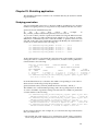
27. Appendix B: Extending GAMOS functionality with C++ utilities ...........245
Converting a Geant4 example into a GAMOS example..............................245
Creating your plug-in .......................................................................................246
Using a parameter in your C++ code .............................................................247
Event classification by interaction types........................................................248
Structure of GAMOS.........................................................................................248
Bibliography ...............................................................................................................251
viii
Chapter 1. Introduction
About this document
This manual refers to GAMOS version 5.0.0. It is written in DocBook and it is
maintained at the following address
http://fismed.ciemat.es/GAMOS/GAMOS_doc/GAMOS.5.0.0/GamosUsersGuide_V5.0.0.pdf
We will use through this manual many terms common to the Monte Carlo simulation terminology and specifically to the Geant4[ 1 ] terminology. If you are new
to it, please read before, for example, the Geant4 documentation [ 2 ]. We have
tried though to make this manual self-consistent, and we hope that, unless you
need a deep knowledge of the Geant4 software, you will not need to refer to any
further documentation.
If you find that some of the instructions given here do not give the expected
result, please use the GAMOS bug report system
http://telemaco.ciemat.es/bugzilla
and detail the problem, the GAMOS version and provide as much information as
possible. We will also warmly welcome any kind of comment or suggestion you
would like to send us about this guide, or about the GAMOS functionalities or
user interface.
If you have some questions about something you do not understand or want to
ask for some new functionality in GAMOS, please use the GAMOS Discussion
Forum
http://groups.google.com/group/gamos_users
Introduction to GAMOS
The acronym GAMOS stands for “Geant4-based Architecture for Medicine-Oriented
Simulations”. It is therefore a Monte Carlo simulation software and it is based
on the Geant4 toolkit [ 1 ]. The objective of GAMOS is to provide a software
framework that serves the unexperienced user to simulate his/her project without having to code in C++ and with a minimal knowledge of Geant4, and at the
same time, let an advanced user add new functionalities and easily integrate it
with the rest of GAMOS functionality.
We have also tried to provide you with several tools that help you understand in
detail your simulation (controlling the verbosity, making histograms about many
variables, scoring different quantities, etc.), as well as other tools to help you in
optimising your simulation. GAMOS is composed of a core software that covers
the main functionality of a Geant4 simulation and a set of applications for specific
domains.
Structure of GAMOS
If you loook into GAMOS.5.0.0 directory you can find several directories. The
directories tmp, lib and bin are internal directories created at GAMOS compilation.
The other directories are the following:
•
source: this is the directory where the GAMOS C++ code lies. You will probably not have to care about this, unless you are an advanced user and need to
develop new code.
•
examples: some first examples. We recommend you that after the GAMOS installation you run the example examples/test/test.in
•
tutorials: you can find nine step-by-step tutorials: Primer, Histogram and Scorers,
PET, SPECT, Compton Camera, Radiotherapy and Shielding, Gamma spectrometry,
plug-in’s. They include several exercises with increasing difficulty, and the exercise outputs as well as the exercise solutions are provided. We recommend you
1
Chapter 1. Introduction
to follow one or several of these tutorials to become acquainted with GAMOS.
The Primer may be a good place to start, as it starts with a few basic examples
and shows how to visualize geometries and histograms.
•
analysis: some utilities that may serve you to analyse your output.
•
data: directory where GAMOS algorithms look for data files (after current directory).
The plug-in concept
To provide the user with a big flexibility in choosing different simulation components (geometry, physics, user actions, histograms, ...) and combining them to
his/her will in a simple way, GAMOS is based on the plug-in concept. This means
that the “main” program runs without predefined components and the user tells
it which components are being loaded at run time (without needing to recompile)
by simply listing them in a text input file. This mechanism also lets the user define
a new component that was not foreseen by GAMOS and easily tell GAMOS to use
it together with any other of his/her own components or GAMOS components.
A common example to better understand the plug-in concept is the plug-in’s that
are installed on your computer when you open some Internet page with your web
browser. Your web browser can use these plug-in’s to get an extra functionality
(viewing videos, animated figures, ...) without your having to recompile it and
even if the web browser designers had never before heard of the new plug-in.
For each of the simulation component types we will describe in the corresponding section which is the command to select it and how to transform a new user
component into a GAMOS plug-in.
For the implementation of plug-in’s GAMOS has chosen the CERN package
ROOT.
2
Chapter 2. Getting started
This chapter explains the practical details to obtain the GAMOS code, compile
and run it.
Getting the code and installing it
GAMOS has been tested in over ten Linux and MacOS distributions and compilers, and in Windows XP and Windows 7 with Visual Studio 2010. Each new
release is tested with over sixty tests in at least three different operating systems.
You can download GAMOS from http://fismed.ciemat.es/GAMOS
GAMOS depends on Geant4 and on ROOT[ 5 ]. To download and install everything you can follow the instruction in the ’Code download’ area.
Installing in Linux and Mac OS
As explained in the web page you need to get first the installation scripts and
uncompress them in the scripts directory (you may do it automatically by downloading the scripts installation utility from the web page). After that you just need
to type the command
./installGamos.sh MY_INSTALLATION_DIR
where MY_INSTALLATION_DIR is the directory where you want to install
GAMOS. The directory name has to be an absolute path, i.e. starting with /.
$HOME is OK because it means /home/.....
This command will download the GAMOS code as well as Geant4 and ROOT
packages, and will compile them all. Be sure that you have installed in your
system the X11 libraries in the directory /usr/X11R6/lib or /usr/local/lib or /usr/lib
(check for the following libraries: libXmu.so , libXt.so, libXext.so, libX11.so,
libICE.so. 1 as well as the OpenGL libraries (check for the following libraries:
libGL.so, libGLU.so). If the OpenGL libraries are not found, GAMOS will ask you
if you want to continue without them. In case of positive answer, GAMOS will
be installed without OpenGLX visualisation (but still with VRML visualisation).
If the X11 libraries are not found, GAMOS will ask you if you want to continue
without them. In case of positive answer, GAMOS will be installed without
OpenGLX visualisation (but still with VRML visualisation) and without ROOT
histograms. ROOT has some extra checks for libraries, namely libXpm.so,
libXft.so and libXi.so, so you also have to install them.
After all the code is compiled, follow the instructions on how to run an example.
If the installation fails, you can find the cause of it in the file install.log at the
directory where you tried to do the installation. Look for the first occurrence of
the characters error (with a blank space first, as several class name have these
characters). It is likely that the error is due to the fact that you are using a ROOT
version not compatible with your system. If this is the case, try to find a new
version number at the ROOT web page htt://root.cern.ch and change it at the file
installGamosBaseDefs.sh that you will find at the scripts directory. Use an older
version if you think your operative system is old and a new version if you think it
is old. If you still are not able to install successfully GAMOS, please open a report
at the GAMOS Users’ Forum, https://groups.google.com/forum/#!forum/gamos_users,
and attach the install.log file (compress it first).
Tips for installation in Ubuntu
If you are using the Ubuntu Linux distribution you have to take into account
that the default installation does not include the software for C++ developement. Therefore, if you do not have this software in your installation youd should
download the following packages:
•
g++
3
Chapter 2. Getting started
•
libcxxtools-dev
•
libx11-dev
•
libxmu-dev
•
libxi-dev
•
libxft-dev
•
libxpm-dev
•
libxext-dev
•
freeglut-dev
•
dpkg-dev
Tips for installation in Fedora Core
If you are using the Fedora Core Linux distribution you have to select the software development tools at your installation. If you do not have this software in
your installation youd should download the following packages:
•
gcc-c++
•
libX11-devel
•
libXmu-devel
•
libXi-devel
•
libSM-devel
•
libICE-devel
•
freeglut-dev (this package has some dependency problems, so you should select the option --skip-broken)
•
libXft-devevl
•
libXpm-devel
Downloading the files separately and installing afterwards
If you have poor connection it may be better to download the GAMOS installation files one by one first and then running the installation process. You have to
download the following files:
•
GAMOS.5.0.0.tgz
•
geant4.9.6.p02.gamos.tar.gz
•
geant4.9.6.p02.gamos.data.tar.gz
•
root_v5.34.10.source.tar.gz
Put all the files in a directory, and then type
./installGamos.sh MY_INSTALLATION_DIR MY_DOWNLOAD_DIR
where MY_INSTALLATION_DIR is the directory where you want to install
GAMOS and MY_DOWNLOAD_DIR is the directory where you copied the
installation files. Both directory names have to be absolute paths, i.e. starting
with /. $HOME is OK because it means /home/.....
Copying GAMOS to a different place
If you have GAMOS installed at a given directory in a given computer and you
want to copy it to another directory or to another computer, you can skip the
downloading phase and go directly to the compilation (you should not try to
use the original GAMOS distribution unless you are sure that the new computer
4
Chapter 2. Getting started
has exactly the same operative system and the directory is the same as in the old
computer). To reinstall without downloading use the command:
./reInstallGamos.sh MY_INSTALLATION_DIR
where MY_INSTALLATION_DIR is the directory where you have copied
GAMOS. The directory name has to be an absolute path, i.e. starting with /.
$HOME is OK because it means /home/.....
Installing in Windows
The first thing to do to install in Windows is selecting a directory, which
we will call MY_INSTALLATION_DIR, and which can be for example
c:\gamos . Before installing GAMOS you have to install ROOT. Get the
executable file from the GAMOS web page and install it. GAMOS has to
know automatically where ROOT is, so be careful not to use the Standard
installation, but the Custom one, and change the default directory, to the
directory MY_INSTALLATION_DIR\external\root\5.34.10\root.
To install GAMOS you have to download the GAMOS.5.0.0.zip file, copy it to
your MY_INSTALLATION_DIR and uncompress it. If your windows system does
not have an unzip software and you do not have one, you may download a
free one from http://7zip.com. After it is decompressed you just have to open
the file MY_INSTALLATION_DIR/GAMOS.5.0.0/GAMOSGUI.exe. The first time
it is opened it will configure GAMOS and create a GAMOSGUI.ini file. To run
GAMOS you just have to select your input file clicking on the Open Input File and
run it clicking on the Run button. All the output files will be written in the same
directory where the input file is.
Checking your windows installation
As explained above, it is mandatory that the directory structure is
correct, so that the GAMOS executable cna find all the dynamic libraries.
You should check that ROOT has been installed in the directory
MY_DIRECTORY/external/root/5.34.10/root while GAMOS has been installed at
MY_DIRECTORY/GAMOS.5.0.0/GAMOSGUI.exe, where MY_DIRECTORY is the
directory you chose for GAMOS.
If the directory structure is OK, the first time you execute GAMOSGUI.exe, it does
not find any file named GAMOSGUI.ini and then a command prompt window (a
black window) pops up. This windows should stay for about 1 minute or more,
and you should see a list of messages telling you that the GAMOS libraries are
being processed. If the black window disappears quickly is that the library processing is giving some error message. In this case you probably are not able to
read the messages fast enough before the windows disappears, so you should try
to process the libraries in other way:
•
Open a command prompt window. In windows XP.
•
Type c:, or the disk unit where the GAMOS directories lie
•
Type cd MY_DIRECTORY where MY_DIRECTORY is the directory where
GAMOSGUI.exe lies
•
Type cd config
•
Type genmap.win.bat > genmap.log
•
Open the genmap.log, for example with more genmap.log, or send this file to the
GAMOS developers if you need help
5
Chapter 2. Getting started
Running an example in Linux or Mac OS
If you have done a standard installation, you will have your code compiled and
ready to run.
Before running any example you have to set some configuration variables, mainly
where you have installed GAMOS and the depending libraries. This is all done
in the file
MY_GAMOS_DIR/config/confgamos.sh 2
or
MY_GAMOS_DIR/config/confgamos.csh
Therefore before running you have to source this file:
source MY_GAMOS_DIR/config/confgamos.sh
or
source MY_GAMOS_DIR/config/confgamos.csh
depending on your shell flavour. Remember to type this command every time you
start a new session to run GAMOS.
To run your application inside GAMOS you do not have to write a “main”
program, as GAMOS provides a unique “main” that serves to run any
application.When you run the GAMOS “main” it will load and call the
components you want (geometry, physics, generator, hits building, histograms,
...) by simply defining them in the input command file. Therefore to run your
application simply type
gamos MY_INPUT_FILE
where MY_INPUT_FILE is a typical Geant4 macro file that includes Geant4 and
GAMOS commands.
The minimum set of commands that you need are those to select a geometry, a
physics list and a generator, to initialize Geant4 and to run N events. In this case
your input file may look like this one:
/gamos/setParam GmGeometryFromText:FileName test.geom
/gamos/geometry GmGeometryFromText
/gamos/physicsList GmEMPhysics
/gamos/generator GmGenerator
/gamos/generator/addSingleParticleSource MY_SOURCE e- 1*MeV
/run/initialize
/run/beamOn 10
This will create a simple geometry, the one described in the file test.geom lying in
the current directory or in the MY_GAMOS_DIR/data directory, set the physics
as the low energy electromagnetic Geant4 physics and run 10 events with an electron of 1 MeV as primary particle.
You can then add any of the command described in this document, or any Geant4
command or any command you created yourself.
Beware that Geant4 is a state machine, and the list of available commands depends on the current state. The main state change is triggered by the /run/initialize
command, which changes the state from G4State_PreInit to G4State_Idle. You may
get a full list of the available commands at any moment with the command /control/manual.
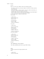
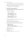
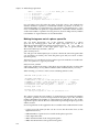
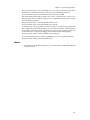
Running an example in Windows
To run in Windows we recommmend you to use the Graphical User Interface,
that you can find at MY_INSTALLATION_DIR/GAMOS.5.0.0/GAMOSGUI.exe.
6
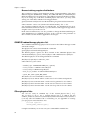
Chapter 2. Getting started
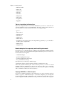
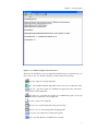
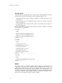
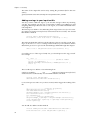
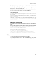
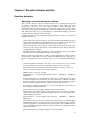
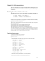
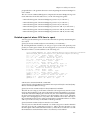
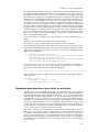
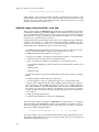
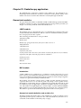
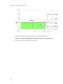
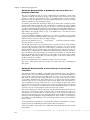
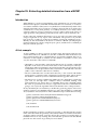
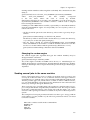
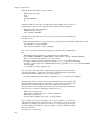
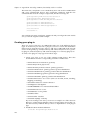
Figure 2-1. GAMOS Graphical User Interface
The first you should do is open an input file and then run it. Or alternatively you
may create a new one. The list of buttons of this GUI is the following:
•
Open File: Open an existing input file
•
Run : run GAMOS with the input file in the screen (it is saved before run)
•
Open Log: open the log file of a GAMOS run (gamos.log in the same directory that the current intput file
•
Open Error Log : open the error log file of a GAMOS run (gamos_error.log in
the same directory that the current intput file
•
New File: create a new input file
•
Save File: save current input file using current name
•
Save File As: save current input file changing name
•
Select Font: select the font for input and log files
•
Help: open the pdf file of GAMOS User’s Guide
7
Chapter 2. Getting started
Exit: exit GUI
•
Compiling GAMOS
If you installed GAMOS as explained in the previous section, the compilation will
be done automatically. Then you may run your application in GAMOS by writing
your user commands without any need of compiling ever more, and therefore
you do not need to read this section.
Only if you want to extend the GAMOS functionality by providing new code,
you will have to follow the instructions in this section.
GAMOS uses the GNU make tool to manage the compilation and generation
of executables. It uses a set of configuration files based on the Geant4 ones.
Therefore, if you are familiar to Geant4, you will find no difficulty in compiling
GAMOS.
After untarring the installation file, you will have a directory called
MY_GAMOS_DIR (substitute it by whatever name you used). This is the
directory where the GAMOS code is, the rest are the external libraries used by
GAMOS and the configuration utilities.
Before compiling, you have to define a few variables, mainly the location of the
different external packages. All this is done by sourcing the file
source MY_GAMOS_DIR/config/confgamos.sh
or
source MY_GAMOS_DIR/config/confgamos.csh
To compile any directory of GAMOS, and all the directories below, you just have
to go to that directory and type make. This will compile all the .cc files found in the
src directory, build the library and the plug-in’s, and in the case of the directory
GamosCore/GamosApplication it will also create the gamos executable. You may
need to type the Linux command rehash to refresh your environmental variables
in case there was no executable file before starting the compilation.
Compiling your new code
If you have created a new directory with your C++ code you have to compile it
following the Geant4 way. The implementation files should have the suffix .cc and
should be in a subdirectory called src. For the declaration files, you have a greater
freedom; the Geant4 way is that they have the suffix .hh and lie in a subdirectory
called include, but you can do it your own way (and after that, you have to be
consistent in the GNUmakefile, as explained below).
You then have to build a GNUmakefile, that will steer the compilation and the
buidling of the libray and the plug-in’s, when you type the command make. For
building it you may follow the examples in the GamosCore/GamosXXX directories.
We take as example the file GamosCore/GamosGeometry/GNUmakefile:
name := GamosGeometry
G4TARGET := $(name)
G4EXLIB := true
.PHONY: all
all: lib plugin
include $(GAMOSINSTALL)/config/binmake.gmk
include $(GAMOSINSTALL)/config/general.gmk
EXTRALIBS += -lGamosBase_Base -lGamosUtils -lGamosUserActionMgr
8
Chapter 2. Getting started
Let’s go one by one through the lines: In the first one you define the name of your
library:
name := GamosGeometry
The following two lines are used internally by the GAMOS scripts and are
mandatory:
G4TARGET := $(name)
G4EXLIB := true
Then you define what you want to do when you type make:
.PHONY: all
all: lib plugin
There are several possibilities:
•
lib Compile and build the library.
•
plugin Build the plug-in. Use it if and only if you are creating a new plug-in.
•
plugin_check Check that you are linking with all the libraries that will be
needed. This check is not mandatory, but if you do not do it and you are
missing some library, when you run you will get an error message.
•
bin Build the executable. You will probably never need this, as GAMOS is based
on dynamic loading and plug-in’s, so that there is only one GAMOS executable,
which is built at installation.
The following two lines are needed for configuration
include $(GAMOSINSTALL)/config/binmake.gmk
include $(GAMOSINSTALL)/config/general.gmk
If you edit the file general.gmk, you will see that it is just including a different file
for each package. Therefore, instead of using it, you may include all or only a
subset of them if you do not need them all.
Finally, you define the GAMOS libraries that will be linked to yours, i.e. the libraries of each of the files that you have included in your code 3
EXTRALIBS += -lGamosBase -lGamosUtils
-lGamosFactories -lGamosUserActionMgr
If you have doubts about which GAMOS libraries to include, you may include
them all, by including include $(GAMOSINSTALL)/config/gamos_libraries.gmk.
If you have built several levels of directories you may want to have the possibility
of typing make at the top most directory to trigger the compilation of all the directories. To do this you just have to add a GNUmakefile at the top level directory
similar to the one at $(GAMOSINSTALL)/source/GamosCore/GNUmakefile, that we
reproduce here:
include $(GAMOSINSTALL)/config/architecture.gmk
SUBDIRS = GamosUtils GamosBase GamosUserActionMgr GamosData
GamosAnalysis GamosGeometry GamosMovement GamosPhysics
GamosGenerator GamosSD GamosUtilsUA GamosReadDICOM
GamosScoring GamosApplication
include $(GAMOSINSTALL)/config/globlib.gmk
9
Chapter 2. Getting started
You only have to change the line starting by SUBDIRS =, to list the name of your
subdirectories.
Notes
1. You may type for example ’locate libXmu.so’ to know where they are in they
are not in the mentioned directories
2. By MY_GAMOS_DIR we mean the installation directory you have chosen,
i.e. MY_INSTALLATION_DIR, plus the directory where the GAMOS version
is installed, i.e.MY_INSTALLATION_DIR/GAMOS.5.0.0
3. For the external packages the set of libraries is fixed and defined in the configuration files
10
Chapter 3. Geometry
You can describe your detector in three different ways: by defining your
setup in a text file, by using one of the geometry examples provided or
in the standard Geant4 way, by writing your C++ class inheriting from
G4VUserDetectorConstruction.
Building your geometry with a text file
You can define your geometry in a simple text file as described in the following
subsection. 1
You can also use as example the one at
MY_GAMOS_DIR/data/test.geom
Once your file is ready, you have to tell GAMOS to use your geometry definition,
first telling the name of your file with the command
/gamos/setParam GmGeometryFromText:FileName MY_FILENAME 2
and then telling GAMOS to use the constructor of geometry from text file
/gamos/geometry GmGeometryFromText
Description of geometry text file format
The description of the geometry is based on tags. A tag is a word that appears at
the first one in a line and sets what the line means.
There are no constraints on the order of the tags in the file, except some logical
restrictions, e.g. a volume cannot be positioned or given attributes if it has not
been defined (e.g. no ’:PLACE’, ’:VIS’, ’:COLOUR’, ’:CHECK_OVERLAPS’ tags
before ’:VOLU’ tag).
We will explain in this section the tags used to describe the geometry, also explaining the meaning of each of the words that follow the tag, and an example of
each tag. Tags can be given with any combination of upper case and lower case
letters. Each tag has a fixed number of arguments, known by the parser; therefore
you may write all arguments in a line or in several lines at your will.
Isotope
:ISOT
•
Name
•
Z
•
N
•
A
Example: :ISOT Cl35 17 18 35.
Element made of one unique isotope
:ELEM
•
Name
•
Symbol
•
Z
•
A
Example: :ELEM Hydrogen H 1. 1.
11
Chapter 3. Geometry
Element composed of several isotopes
:ELEM_FROM_ISOT
•
Name
•
Symbol
•
Number of components
One line per isotope with
•
isotope name
•
fraction of number of atoms per volume
Example: :ELEM_FROM_ISOT Chlorine Cl 2 Cl35 0.4 Cl36 0.6
Material made of one element
:MATE
•
Name
•
Z
•
A
•
Density
Example: :MATE Iron 26. 55.85 7.87
Material made of a mixture of elements or materials
:MIXT
•
Name
•
Density
•
Number of components
One line per material or element with
•
material name
•
proportion of material in the mixture
The components can be either all elements or all materials, but both types cannot
appear in the same mixture.
There are three mixture tags, depending of the way the proportions are defined:
•
Proportions by weight fractions
:MIXT_BY_WEIGHT
This tag is equivalent to the ":MIXT" tag
•
Proportions by number of atoms
:MIXT_BY_NATOMS
•
Proportions by volume
:MIXT_BY_VOLUME
The first two tags can be used to build material mixtures out of elements or materials, but the last tag can only be applied with material components (elements
do not have density).
Example:
12
Chapter 3. Geometry
:MIXT Fiber_Lead
9.29
Lead
0.9778
Polystyrene 0.0222
2
:MIXT_BY_NATOMS CO2 1.8182E-3 2
C 1
O 2
:MIXT_BY_VOLUME H-CO2 (1.214E-03+1.8182E-3)/2. 2
Hydrogen 0.5
CO2 0.5
Material properties
:MATE_MEE
•
Material name
•
Mean excitation energy
Example: :MATE_MEE G4_WATER 10.*eV
:MATE_STATE
•
Material name
•
State: Undefined / Solid / Liquid / Gas
If material is not set, it is Undefined.
Example: :MATE_STATE G4_WATER Solid
:MATE_TEMPERATURE
•
Material name
•
Temperature
If temperature is not set, it is STP, i.e. 273.15 kelvin. The default unit of temperature is kelvin
Example: :MATE_TEMPERATURE G4_WATER 293.15*kelvin // 20 oC
:MATE_PRESSURE
•
Material name
•
Pressure
If pressure is not set, it is STP, i.e. 1 atmosphere. The default unit of temperature
is atmosphere
Example: :MATE_PRESSURE G4_WATER 1.5*bar
Geant4 internal database of materials and elements
Geant4 provides a list of predefined materials, whose compositions correspond
to the NIST definition [ 13 ]. Among them you can find all single elementary
materials, from Z = 1 (Hydrogen) to Z = 98 (Californium). You can use those
materials when building a volume without the need to redefine them on your
ASCII (= text) file. It is just enough that the material name you assign to a volume corresponds to the name of one of these predefined materials (they all start
13
Chapter 3. Geometry
with “G4_”). The Geant4 materials have the mean excitation energy set explicitly, instead of allowing an automatic calculation from its components. You may
override those materials if you want, by redefining them in your ASCII file.
Also Geant4 provides the definition of all elements from Z = 1 (Hydrogen) to Z =
107 (Bohrium). Their names are the usual symbol in the periodic table of elements
(no “G4_”). These elements take into account the isotope composition.
you can find the details of the NIST materials composition in the Geant4 file:
source/materials/src/G4NistMaterialBuilder.cc
The full list is the following:
G4_A-150_TISSUE,
G4_ACETONE,
G4_ACETYLENE,
G4_ADENINE,
G4_ADIPOSE_TISSUE_ICRP,
G4_AIR,
G4_ALANINE,
G4_ALUMINUM_OXIDE,
G4_AMBER,
G4_AMMONIA,
G4_ANILINE,
G4_ANTHRACENE,
G4_B-100_BONE,
G4_BAKELITE,
G4_BARIUM_FLUORIDE,
G4_BARIUM_SULFATE,
G4_BENZENE,
G4_BERYLLIUM_OXIDE,
G4_BGO,
G4_BLOOD_ICRP,
G4_BONE_COMPACT_ICRU,
G4_BONE_CORTICAL_ICRP,
G4_BORON_CARBIDE,
G4_BORON_OXIDE,
G4_BRAIN_ICRP,
G4_BUTANE,
G4_N-BUTYL_ALCOHOL,
G4_C-552,
G4_CADMIUM_TELLURIDE,
G4_CADMIUM_TUNGSTATE,
G4_CALCIUM_CARBONATE,
G4_CALCIUM_FLUORIDE,
G4_CALCIUM_OXIDE,
G4_CALCIUM_SULFATE,
G4_CALCIUM_TUNGSTATE,
G4_CARBON_DIOXIDE,
G4_CARBON_TETRACHLORIDE,
G4_CELLULOSE_CELLOPHANE,
G4_CELLULOSE_BUTYRATE,
G4_CELLULOSE_NITRATE,
G4_CERIC_SULFATE,
G4_CESIUM_FLUORIDE,
G4_CESIUM_IODIDE,
G4_CHLOROBENZENE,
G4_CHLOROFORM,
G4_CONCRETE,
G4_CYCLOHEXANE,
G4_1, 2-DICHLOROBENZENE,
G4_DICHLORODIETHYL_ETHER,
G4_1,2-DICHLOROETHANE,
G4_DIETHYL_ETHER,
G4_N, N-DIMETHYL_FORMAMIDE,
G4_DIMETHYL_SULFOXIDE,
G4_ETHANE,
G4_ETHYL_ALCOHOL,
G4_ETHYL_CELLULOSE,
G4_ETHYLENE,
G4_EYE_LENS_ICRP,
14
Chapter 3. Geometry
G4_FERRIC_OXIDE,
G4_FERROBORIDE,
G4_FERROUS_OXIDE,
G4_FERROUS_SULFATE,
G4_FREON-12,
G4_FREON-12B2,
G4_FREON-13,
G4_FREON-13B1,
G4_FREON-13I1,
G4_GADOLINIUM_OXYSULFIDE,
G4_GALLIUM_ARSENIDE,
G4_GEL_PHOTO_EMULSION,
G4_Pyrex_Glass,
G4_GLASS_LEAD,
G4_GLASS_PLATE,
G4_GLUCOSE,
G4_GLUTAMINE,
G4_GLYCEROL,
G4_GUANINE,
G4_GYPSUM,
G4_N-HEPTANE,
G4_N-HEXANE,
G4_KAPTON,
G4_LANTHANUM_OXYBROMIDE,
G4_LANTHANUM_OXYSULFIDE,
G4_LEAD_OXIDE,
G4_LITHIUM_AMIDE,
G4_LITHIUM_CARBONATE,
G4_LITHIUM_FLUORIDE,
G4_LITHIUM_HYDRIDE,
G4_LITHIUM_IODIDE,
G4_LITHIUM_OXIDE,
G4_LITHIUM_TETRABORATE,
G4_LUNG_ICRP,
G4_M3_WAX,
G4_MAGNESIUM_CARBONATE,
G4_MAGNESIUM_FLUORIDE,
G4_MAGNESIUM_OXIDE,
G4_MAGNESIUM_TETRABORATE,
G4_MERCURIC_IODIDE,
G4_METHANE,
G4_METHANOL,
G4_MIX_D_WAX,
G4_MS20_TISSUE,
G4_MUSCLE_SKELETAL_ICRP,
G4_MUSCLE_STRIATED_ICRU,
G4_MUSCLE_WITH_SUCROSE,
G4_MUSCLE_WITHOUT_SUCROSE,
G4_NAPHTHALENE,
G4_NITROBENZENE,
G4_NITROUS_OXIDE,
G4_NYLON-8062,
G4_NYLON-6/6,
G4_NYLON-6/10,
G4_NYLON-11_RILSAN,
G4_OCTANE,
G4_PARAFFIN,
G4_N-PENTANE,
G4_PHOTO_EMULSION,
G4_PLASTIC_SC_VINYLTOLUENE,
G4_PLUTONIUM_DIOXIDE,
G4_POLYACRYLONITRILE,
G4_POLYCARBONATE,
G4_POLYCHLOROSTYRENE,
G4_POLYETHYLENE,
G4_MYLAR,
G4_PLEXIGLASS,
G4_POLYOXYMETHYLENE,
G4_POLYPROPYLENE,
G4_POLYSTYRENE,
G4_TEFLON,
15
Chapter 3. Geometry
G4_POLYTRIFLUOROCHLOROETHYLENE,
G4_POLYVINYL_ACETATE,
G4_POLYVINYL_ALCOHOL,
G4_POLYVINYL_BUTYRAL,
G4_POLYVINYL_CHLORIDE,
G4_POLYVINYLIDENE_CHLORIDE,
G4_POLYVINYLIDENE_FLUORIDE,
G4_POLYVINYL_PYRROLIDONE,
G4_POTASSIUM_IODIDE,
G4_POTASSIUM_OXIDE,
G4_PROPANE,
G4_lPROPANE,
G4_N-PROPYL_ALCOHOL,
G4_PYRIDINE,
G4_RUBBER_BUTYL,
G4_RUBBER_NATURAL,
G4_RUBBER_NEOPRENE,
G4_SILICON_DIOXIDE,
G4_SILVER_BROMIDE,
G4_SILVER_CHLORIDE,
G4_SILVER_HALIDES,
G4_SILVER_IODIDE,
G4_SKIN_ICRP,
G4_SODIUM_CARBONATE,
G4_SODIUM_IODIDE,
G4_SODIUM_MONOXIDE,
G4_SODIUM_NITRATE,
G4_STILBENE,
G4_SUCROSE,
G4_TERPHENYL,
G4_TESTES_ICRP,
G4_TETRACHLOROETHYLENE,
G4_THALLIUM_CHLORIDE,
G4_TISSUE_SOFT_ICRP,
G4_TISSUE_SOFT_ICRU-4,
G4_TISSUE-METHANE,
G4_TISSUE-PROPANE,
G4_TITANIUM_DIOXIDE,
G4_TOLUENE,
G4_TRICHLOROETHYLENE,
G4_TRIETHYL_PHOSPHATE,
G4_TUNGSTEN_HEXAFLUORIDE,
G4_URANIUM_DICARBIDE,
G4_URANIUM_MONOCARBIDE,
G4_URANIUM_OXIDE,
G4_UREA,
G4_VALINE,
G4_VITON,
G4_WATER,
G4_WATER_VAPOR,
G4_XYLENE,
G4_GRAPHITE,
G4_lH2,
G4_lN2,
G4_lO2,
G4_lAr,
G4_lKr,
G4_lXe,
G4_PbWO4,
G4_Galactic
Other materials common in medical physics are also predefined
in
the
files
MY_GAMOS_DIR/data/NIST_materials.txt
and
MY_GAMOS_DIR/data/PET_materials.txt.
The full list is the following:
BaF2
BaI2
BGO
CdTe
16
Chapter 3. Geometry
CdWO4
CZT
CeBr3
CeCl3
CsI
GaAs
Gd2O2S
GSO
HgI2
LaBr3
LaCl3
LiF
Li2B4O7
LSO
LYSO
LuAG
LuAP
LuYAP
LuI3
NaI
PbWO4
SrI2
YAG
YAPNIST_Al2O3
NIST_Barite
NIST_BaSO4
NIST_CaO
NIST_Concrete
NIST_PMMA
NIST_PVC
NIST_Adipose Tissue (ICRU-44)
NIST_Blood, Whole (ICRU-44)
NIST_Bone, Cortical (ICRU-44)
NIST_Brain, Grey/White Matter (ICRU-44)
NIST_Breast Tissue (ICRU-44)
NIST_Cadmium Telluride
NIST_15 mmol L-1 Ceric Ammonium Sulfate Solution
NIST_Concrete, Ordinary
NIST_Concrete, Barite (TYPE BA)
NIST_Eye Lens (ICRU-44)
NIST_Ferrous Sulfate Standard Fricke
NIST_Gafchromic Sensor
NIST_Lung Tissue (ICRU-44)
NIST_Muscle, Skeletal (ICRU-44)
NIST_Ovary (ICRU-44)
NIST_Photographic Emulsion (Kodak Type AA)
NIST_Polyethylene Terephthalate, (Mylar)
NIST_Polymethyl Methacrylate
NIST_Polytetrafluoroethylene, (Teflon)
NIST_Radiochromic Dye Film, Nylon Base
NIST_Testis (ICRU-44)
NIST_Tissue, Soft (ICRU-44)
Solids
:SOLID
•
solid name
•
solid type name
•
... List of solid parameters
The meaning and order of the solid parameters is the same as in the corresponding Geant4 solid constructor. All the Geant4 CSG and "specific" solids are implemented. The list of solid types and the corresponding parameters is the following
(for better understanding of the solid parameters meaning we refer to the Geant4
user’s manual [ 7 ]):
BOX: box
17
Chapter 3. Geometry
•
X Half-length
•
Y Half-length
•
Z Half-length
TUBE: tube
•
Inner radius
•
Outer radius
•
Half length in z
TUBS: tube section
•
Inner radius
•
Outer radius
•
Half length in z
•
Starting phi angle
•
Delta (=size) phi angle of the segment
CONE: cone
•
Inner radius at -fDz
•
Outer radius at -fDz
•
Inner radius at +fDz
•
Outer radius at +fDz
•
Half length in z (=fDz)
CONS: cone section
•
Inner radius at -fDz
•
Inner radius at +fDz
•
Outer radius at -fDz
•
Outer radius at +fDz
•
Half length in z (=fDz)
•
Starting phi angle of the segment
•
Delta (=size) phi angle of the segment
TRD: trapezoid
•
Half-length along x at the surface positioned at -dz
•
Half-length along x at the surface positioned at +dz
•
Half-length along y at the surface positioned at -dz
•
Half-length along y at the surface positioned at +dz
•
Half-length along z axis
PARA: parallelepiped
18
•
Half-length in x
•
Half-length in y
•
Half-length in z
•
Angle formed by the y axis and by the plane joining the centre of the faces
G4Parallel to the z-x plane at -dy and +dy
•
Polar angle of the line joining the centres of the faces at -dz and +dz in z
•
Azimuthal angle of the line joining the centres of the faces at -dz and +dz in z
Chapter 3. Geometry
TRAP: generic trapezoid
•
Half-length along the z-axis (=pDz)
•
Polar angle of the line joining the centres of the faces at -/+pDz
•
Azimuthal angle of the line joining the centre of the face at -pDzto the centre of
the face at +pDz
•
Half-length along y of the face at -pDz (=pDy1)
•
Half-length along x of the side at y=-pDy1 of the face at -pDz
•
Half-length along x of the side at y=+pDy1 of the face at -pDz
•
Angle with respect to the y axis from the centre of the side at y=-pDy1 to the
centre at y=+pDy1 of the face at -pDz
•
Half-length along y of the face at +pDz (=pDy2)
•
Half-length along x of the side at y=-pDy2 of the face at +pDz
•
Half-length along x of the side at y=+pDy2 of the face at +pDz
•
Angle with respect to the y axis from the centre of the side at y=-pDy2 to the
centre at y=+pDy2 of the face at +pDz
or alternatively, if your trapezoid is a simpler one, you can use the parameters
•
Length along z
•
Length along y
•
Length along x at the wider side
•
Length along x at the narrower side
SPHERE: sphere
•
Inner radius
•
Outer radius
•
Starting phi angle of the segment
•
Delta (=size) phi angle of the segment
•
Starting theta angle of the segment
•
Delta (=size) theta angle of the segment
ORB: full solid sphere
•
Outer radius
TORUS: torus
•
Inside radius
•
Outside radius
•
Swept radius of torus
•
Starting phi angle (fSPhi+fDPhi <= 2PI, fSPhi > -2PI)
•
Delta (=size) phi angle of the segment
POLYCONE: polycone
•
Phi starting angle
•
Delta (=size) phi angle
•
Number of z planes or Number of rz points
For each z plane:
•
Position of z plane
19
Chapter 3. Geometry
•
Tangent distance to inner surface
•
Tangent distance to outer surface
For each rz corner:
•
R coordinate of these corners
•
Z coordinate of these corners
The software will know which if the numbers refer to plane or rz points by looking at the number of parameters provided and comparing it with the number
expected
Example:
:SOLID polyc POLYCONE 0 360 6
3 -2
3.5 -2
3.5 0.75
3.75 1
3.75 2
32
or equivalently
:SOLID polyc POLYCONE 0 360 4
-2 3 3.5
0.75 3 3.5
1. 3. 3.75
2. 3. 3.75
POLYHEDRA: polyhedra
•
Phi starting angle
•
Delta (=size) phi angle
•
Number of sides
•
Number of z planes or Number of rz points
For each z plane:
•
Position of z plane
•
Tangent distance to inner surface
•
Tangent distance to outer surface
For each rz corner:
•
R coordinate of these corners
•
Z coordinate of these corners
The software will know which if the numbers refer to plane or rz points by looking at the number of parameters provided and comparing it with the number
expected
Example:
:SOLID polyh POLYHEDRA 20. 180. 3 4
1900. 32.
1800. 30
1800. 0.
20
Chapter 3. Geometry
1900. 0.
or equivalently
:SOLID polyh POLYHEDRA 20. 180. 3 2
1800. 0. 30.
1900. 0. 32.
ELLIPTICALTUBE: elliptical tube
•
Half length X
•
Half length Y
•
Half length Z
ELLIPSOID: ellipsoid
•
Semiaxis in X
•
Semiaxis in Y
•
Semiaxis in Z
•
Lower cut plane level, z
•
Upper cut plane level, z
ELLIPTICALCONE: elliptical cone
•
Semiaxis in X
•
Semiaxis in Y
•
Height of elliptical cone
•
Upper cut plane level
HYPE: hyperbolic profile
•
Inner radius
•
Outer radius
•
Inner stereo angle
•
Outer stereo angle
•
Half length in Z
TET: tetrahedron
•
Anchor point
•
Point 2
•
Point 3
•
Point 4
•
Flag indicating degeneracy of points
TWISTEDBOX: box twisted along one axis
•
Twist angle
•
Half x length
•
Half y length
21
Chapter 3. Geometry
•
Half z length
TWISTEDTRAP: trapezoid twisted along one axis
•
Twisted angle
•
Half x length at y=-pDy
•
Half x length at y=+pDy
•
Half y length (=pDy1)
•
Half z length (=pDz)
•
Polar angle of the line joining the centres of the faces at -/+pDz
•
Half y length at -pDz (=pDy2)
•
Half x length at -pDz, y=-pDy1
•
Half x length at -pDz, y=+pDy1
•
Half y length at +pDz
•
Half x length at +pDz, y=-pDy2
•
Half x length at +pDz, y=+pDy2
•
Angle with respect to the y axis from the centre of the side
TWISTEDTRD: twisted trapezoid with the x and y dimensions varying along z
•
Half x length at the surface positioned at -pDz
•
Half x length at the surface positioned at +pDz
•
Half y length at the surface positioned at -pDz
•
Half y length at the surface positioned at +pDz
•
Half z length (=pDz)
•
Twisted angle
TWISTEDTUBS: tube section twisted along its axis
•
Twisted angle
•
Inner radius at end-cap
•
Outer radius at end-cap
•
Half z length
•
Phi angle of a segment
BREPBOX: Boundary REPresented box
•
Point 1 X
•
Point 1 Y
•
Point 1 Z
•
Point 2 X
•
Point 2 Y
•
Point 2 Z
•
...
•
Point 8 X
•
Point 8 Y
•
Point 8 Z
BREPCYLINDER: Boundary REPresented cylinder
•
22
Origin X
Chapter 3. Geometry
•
Origin Y
•
Origin Z
•
Axis X
•
Axis Y
•
Axis Z
•
Direction X
•
Direction Y
•
Direction Z
•
Radius
•
Length
BREPCYLINDER: Boundary REPresented cylinder
•
Origin X
•
Origin Y
•
Origin Z
•
Axis X
•
Axis Y
•
Axis Z
•
Direction X
•
Direction Y
•
Direction Z
•
Length
•
Small radius
•
Large radius
BREPSPHERE: Boundary REPresented sphere
•
Origin X
•
Origin Y
•
Origin Z
•
Xhat X
•
Xhat Y
•
Xhat Z
•
ZHat X
•
ZHat Y
•
ZHat Z
•
Radius
BREPTORUS: Boundary REPresented torus
•
Origin X
•
Origin Y
•
Origin Z
•
Axis X
•
Axis Y
•
Axis Z
•
Direction X
23
Chapter 3. Geometry
•
Direction Y
•
Direction Z
•
Length
•
Minimum radius
•
Maximum radius
BREPPCONE: Boundary REPresented polycone
•
Phi starting angle
•
Delta (=size) phi angle
•
Number of z planes
•
Starting value of z
For each z plane:
•
Position of z plane
•
Tangent distance to inner surface
•
Tangent distance to outer surface
BREPPOLYHEDRA : Boundary REPresented polyhedra
•
Phi starting angle
•
Delta (=size) phi angle
•
Number of sides
•
Number of z planes
•
Starting value of z
For each z plane:
•
Position of z plane
•
Tangent distance to inner surface
•
Tangent distance to outer surface
TESSELATED : Boundary REPresented polyhedra
•
Number of facets
For each facet:
•
Number of points (must be 3 or 4)
•
Point 1 X
•
Point 1 Y
•
Point 1 Z
•
Point 2 X
•
Point 2 Y
•
Point 2 Z
•
Point 3 X
•
Point 3 Y
•
Point 3 Z
If there are four points:
24
•
Point 4 X
•
Point 4 Y
Chapter 3. Geometry
•
Point 4 Z
•
Type of facet vertex (0 = ABSOULUTE, 1 = RELATIVE)
EXTRUDED : Boundary REPresented polyhedra
•
Number of polygon vertices
For each vertex of the outlined polygon, defined in clock-wise order:
•
X
•
Y
•
Number of Z sections
For each Z section, defined by z position in increasing order:
•
Half length in Z
•
Offset X
•
Offset Y
•
Scale
Boolean solids
The three types of Geant4 boolean solids are supported: union, subtraction and
intersection. The same tag should be used as for normal solids, but putting as
solid type the type of boolean operation. The parameters are
•
Solid name
•
Solid boolean operation (UNION/SUBTRACTION/INTERSECTION)
•
First component solid name
•
Second component solid name
•
Name of relative rotation matrix
•
Relative X position
•
Relative Y position
•
Relative Z position
Example: :SOLID myunion UNION solid1 solid2 RM30 -11.8 12.5 0.
Volumes
There are two ways to define a logical volume. You can build if from a previously
declared solid associating a material to it
:VOLU
•
Volume name
•
Solid name
•
Material name
Example: :VOLU HALL HALL Air
or you can skip the definition of the solid and in one unique line define the solid
and the material (valid also for boolean solids). You should then use the same
format as for the :SOLID tag, but adding as last word the material name
Example:
Instead of
:SOLID HALL BOX 5000. 5000. 20000.
25
Chapter 3. Geometry
:VOLU HALL HALL Air
use
:VOLU HALL BOX 5000. 5000. 20000. Air
Placement of a volume
All the possible ways to place a volume in Geant4 are supported: a single placement, a parameterised one, a division, a replica and an assembly.
Single placement
:PLACE
•
Volume name
•
Copy number
•
Parent volume name
•
Name of rotation matrix
•
X position
•
Y position
•
Z position
Example:
:VOLU yoke :TUBS Iron 3 620. 820. 1270.
:PLACE yoke 1 expHall R00
0.0 0.0
370.
Parameterisation
The parameterisations supported are the placement of several copies of a volume
along a line, in a circle and in a bidimensional grid (other types of parameterisation may be added at user request).
:PLACE_PARAM
•
Volume name
•
Copy number
•
Parent volume name
•
Parameterisation type
•
Name of rotation matrix
•
Number of copies
•
Step (separation between copies)
•
Offset
•
Extra arguments (optional, depend on parameterisation type)
There are three types of linear parameterisations, along the three axis X,Y,Z
(types: LINEAR_X, LINEAR_Y, LINEAR_Z) and a general one (type LINEAR)
for which you have to add as extra arguments the axis direction DIR_X DIR_Y
DIR_Z. The offset for linear parameterisations represents the distance from the
centre of the first copy to the point (0,0,0) along the line.
In the case of circle parameterisation, the circle is around the Z axis by default.
If you want a circle around another axis you can provide as extra arguments the
axis and, optionally, the position of the first copy.
There are three types of square parameterisation, in the planes XY,XZ,YZ (types:
SQUARE_XY, SQUARE_XZ, SQUARE_YZ) and a general one (type SQUARE).
26
Chapter 3. Geometry
For this bidimensional parameterisations you have to provide two copy numbers,
two steps and, optionally, two offsets. For the general case, SQUARE the offset
is not needed, but you have to add as extra arguments the two axis, that do not
have to be orthogonal, and, optionally, the position of the first copy. In the case
of this paramerisation type, you have to provide two number of copies, one for
each axis.
Example:
:PLACE_PARAM mytube 1 subworld2 LINEAR_X RM0 5 20. 0.
:PLACE_PARAM mytube 1 subworld1 LINEAR RM0 5 20. 0. 1. 1. 1. -50. 0. 0.
:PLACE_PARAM mybox 0 mother CIRCLE_XY RM0 30 6*deg 90*deg 15*cm
:PLACE_PARAM mybox 1 subworld2 SQUARE_XZ RM0 5 5 20. 20.
:PLACE_PARAM mybox 1 subworld1 SQUARE RM0 5 8 20. 10. 0. 1. 1. 0. 1. 0.
Be aware that putting offset = 0 means that the first copy is placed at (0,0,0). This
may be not what you want if, for example, you are filling a box with an square
of small boxes using an square parameterisation: offset 0 will mean that all the
copies are placed in the positive-positive quarter of the mother box.
Phantom parameterisation
This is a special case of parameterisation that serves to create a three
dimensional grid of equal voxels. The parameterisation is instantiated as a
G4PhantomParameterisation, so that the G4RegularNavigation algorithm is used for
optimal efficiency in the navigation.
The format of this parameterisation is the following
•
Volume name
•
Copy number
•
Parent volume name
•
Parameterisation type
•
Name of rotation matrix
•
Number of copies in X
•
Number of copies in Y
•
Number of copies in Z
•
Step (separation between copies) in X
•
Step (separation between copies) in Y
•
Step (separation between copies) in Z
Following the rules of G4RegularNavigation the voxels must completely fill the
mother volume, therefore a container volume of appropiate dimensions should
be defined as mother volume, see the example below.
Example:
:VOLU phantom_container BOX 50. 100. 100. G4_WATER
:VOLU phantom BOX 10 10 10 G4_WATER
:PLACE_PARAM phantom 1 phantom_container PHANTOM 5 10 10 20. 20. 20.
27
Chapter 3. Geometry
Division
There are several ways to define a division in Geant4, by giving:
•
the number of divisions (so that the width of each division will be automatically calculated)
•
the division width (so that the number of divisions will be automatically calculated to fill as much of the mother as possible)
•
both the number of divisions and the division width (this is especially designed
for the case where the copies do not fully fill the mother)
To each of these types correspond a different tag
:DIV_WIDTH
•
Volume name
•
Parent volume name
•
Material name
•
Axis of division
•
Division width
•
Offset (not mandatory)
:DIV_NDIV
•
Volume name
•
Parent volume name
•
Material name
•
Axis of division
•
Number of divisions
•
Offset (not mandatory)
:DIV_NDIV_WIDTH
•
Volume name
•
Parent volume name
•
Material name
•
Axis of division
•
Number of divisions
•
Division width
•
Offset (not mandatory)
Example:
:DIV_WIDTH mybox mother AIR Z 10.
:DIV_NDIV_WIDTH mytube mother copper PHI 12 10.*deg
Replica
To define a replica the following tag must be used:
:REPL
28
•
Volume name
•
Parent volume name
Chapter 3. Geometry
•
Axis of division
•
Number of divisions
•
Division width
•
Offset (not mandatory)
Example: :REPL crystal Block X 10 5.*cm
Remember, that different to the divisions, where the solid type and dimensions
are calculated automatically be Geant4, in the case of replicas the volume name
used must be the name of a previously defined volume. This solid is not really
used for navigation but should have the correct type and dimensions for visualisation.
Assembly volumes
Assembly volumes are sets of logical volumes that are combined together, so that
they act as if there were in a real mother, but without creation of the mother.
To define assembly volumes you have to define the relative rotations and positions of all the logical volumes
:VOLU_ASSEMBLY
•
Volume name
•
Number of logical volumes
•
Axis of division
•
Number of divisions
•
Division width
•
Offset (not mandatory)
One line per logical volume with
•
Logical volume name
•
Rotation matrix name
•
position X
•
position Y
•
position Z
Then to place the assembly volume you can use:
:PLACE_ASSEMBLY
•
Volume name
•
Copy number
•
Parent volume name
•
Name of rotation matrix
•
X position
•
Y position
•
Z position
Example:
:SOLID Crystal BOX 10 10 10
:SOLID Crystal2 BOX 5 5 5
:VOLU_ASSEMBLY CrystalSet 3
Crystal RM0 0. 0. 0.
Crystal RM1 0. 0. 20.
Crystal2 RM0 0. 20 -10
:PLACE_ASSEMBLY CrystalSet 1 expHall R00 100.
0.
0.
29
Chapter 3. Geometry
Rotation matrix
A rotation matrix is interpreted as the rotation that should be applied to the object
in the reference system of its mother. It can be defined in three ways:
•
a) By giving the three rotation angles around the X, Y and Z axis (in this order
of rotations)
•
b) By giving the polar and azimuthal angles of the X, Y and Z axis after the
rotation is applied
•
c) By giving the nine matrix elements of the rotation matrix: XX, XY, XZ, YX,
YY, YZ, ZX, ZY, ZZ
The tag for the three cases is the same. The parser will know which case is meant
by the number of parameters.
a) :ROTM
•
Name
•
Angle of rotation around global X axis
•
Angle of rotation around global Y axis
•
Angle of rotation around global Z axis
Example: :ROTM R0 0. 0. 0.
b) :ROTM
•
Name
•
Polar angle for axis X
•
Azimuthal angle for axis X
•
Polar angle for axis Y
•
Azimuthal angle for axis Y
•
Polar angle for axis Z
•
Azimuthal angle for axis Z
Example: :ROTM R0 90. 0. 90. 90. 0. 0.
c) :ROTM
•
Name
•
9 parameters defining the rotation matrix
Example: :ROTM R0 1. 0. 0. 0. 1. 0. 0. 0. 1.
Module
A module is a new concept that simplifies the description of difficult pieces of
a geometry. While these pieces could be built by adding several volumes and
placing them in the correct position, it is sometimes much easier to give a few
parameters that describe them and GAMOS will take care of making all the calculations to create the volumes and place them. The current implementation has
two modules defined: JAWS and MLC (multileaf collimators). See section on RadioTherapy for a detailed description of these modules.
30
Chapter 3. Geometry
Visibility
:VIS
•
Volume name
•
ON or TRUE, OFF or FALSE
Example: :VIS yoke OFF
By default the visibility of all volumes is set to ON
Colour and transparency
To define the colour of a volume
:COLOUR/:COLOR
•
Volume name
•
Red colour proportion
•
Green colour proportion
•
Blue colour proportion
•
Transparency
The four parameters can take a value between 0 and 1. The transparency parameter is not mandatory.
Example: :COLOUR NDC_chamber 0.2 0.4 0.1
By default, the three colour proportions will be set to -1.
Check overlaps
Geant4 offers the possibility to check if a volume overlaps with other volumes.
By default it is not set, but you can activate it with the commands
:CHECK_OVERLAPS
•
Volume name
•
ON or TRUE, OFF or FALSE
Example: :CHECK_OVERLAPS NDC_chamber 0.2 0.4 0.1
By default, the three colour proportions will be set to -1
Use of ’*’ in names
In the case of the :VIS, :COLOUR , :MATE_MEE, :MATE_PRESSURE,
:MATE_TEMPERATURE, :MATE_STATE and :CHECK_OVERLAPS tags, you
may use ’*’ to define the volume or material name. This ’*’ will be replaced by
’any name’. For example Crys* means all the volume names starting by ’Crys’, *
means all volume names.
Use of parameters
You can also define a parameter to set a value for later use in any tag.
:P
•
parameter name
•
parameter value
31
Chapter 3. Geometry
You can then use the parameter as: ’$’ + parameter_name
Example:
:P InnerR 12.
:VOLU yoke :TUBS Iron 3 $InnerR 820. 1270.
Units
Any value in a tag has a default unit that depends on the dimension of the value
(automatically known by the parser). The default units are the following:
•
length: mm
•
angle: degrees
•
density: g/cm3
•
atomic mass: g/mole
•
temperature: kelvin
•
pressure: atmosphere
The user can override the default value of a unit by indicating the unit of each
value. This can be done adding at the end of the value the unit name (see CLHEP
file Units/SystemOfUnits.h) preceded by a ’*’ character; e.g. 3*mm, 1.4*rad,...
Arithmetic Expressions
For any value you want to define in a tag you can use the most common mathematical expressions instead of directly writing the figures, e.g:
3-sin(8.2/3.5)
(3+4)*(7-log(3))
You can also use parameters and units in the expressions, e.g:
7.2*$RADIUS*mm-$X_LENGTH/1.5*cm
If you use a regular expression, remember that there can only be a unit in the
whole expression, and it must be at the end.
The regular expressions used include (their meaning is evident): +, -, *, /, sin, cos
,tan ,asin ,acos ,atan ,atan2 ,sinh ,cosh ,tanh ,sqrt ,exp ,log ,log10 ,pow.
Including other files
You can nest several files by using the #include’ directive anywhere in your geometry files.
Example: #include mygeom2.txt
Combining C++ and ASCII files
If you want to define part of your geometry with C++ and another part with
ASCII files, you should follow these instructions.
Write a C++ class inheriting from G4VuserDetectorConstruction and in the Construct() method build the geometry from a set of ASCII files
32
Chapter 3. Geometry
G4tgbVolumeMgr* volmgr = G4tgbVolumeMgr::GetInstance();
volmgr->AddTextFile(“mifile1.txt”);
volmgr->AddTextFile(“mifile2.txt”);
G4VPhysicalVolume* physiSubWorld =
volmgr->ReadAndConstructDetector();
You can then use the returned G4VPhysicalVolume as the world volume or get its
logical volume and place it inside any other logical volume.
You can also use the materials and volumes of the ASCII geometry in your C++
geometry retrieving them by name. To retrieve the pointer of a material:
GmGeometryUtils* geomUtils = GmGeometryUtils::GetInstance();
// one volume
G4LogicalVolume* world_logic =
(geomUtils->GetLogicalVolumes("world",true))[0];
// several volumes with same name
std::vector < G4LogicalVolume* > crystal_logic =
(geomUtils->GetLogicalVolumes("crystal",exists=true));
To retrieve a logical volume
GmGeometryUtils* geomUtils = GmGeometryUtils::GetInstance();
// one volume
G4LogicalVolume* world_logic =
(geomUtils->GetLogicalVolumes("world",true))[0];
// several volumes with same name
std::vector < G4LogicalVolume* > crystal_logic =
(geomUtils->GetLogicalVolumes("crystal",exists=true));
To retrieve the physical volumes
GmGeometryUtils* geomUtils = GmGeometryUtils::GetInstance();
std::vector < G4VPhysicalVolume* > crystal_phys =
(geomUtils->GetPhysicalVolumes("crystal",exists=true));
You can find an example in the Geant4 examples directory:
examples/extended/persistency/P03/src/
ExTGDetectorConstructionWithCpp.cc
Dumping your Geant4 geometry in text file format
If you have already a Geant4 geometry written with C++ code or any other
method you can get a geometry text file by simply adding a line in your code
G4tgbGeometryDumper::GetInstance()->DumpGeometry(theFileName);
This line should be executed once your geometry has been built, for example in a
BeginOfRunAction method, or at the end of the Construct method in your detector
constructor class.
You can do this in GAMOS by simply adding in your command file the user
action named GmGeomTextDumperUA:
/gamos/userAction GmGeomTextDumperUA
33
Chapter 3. Geometry
The name of the output file can be set by setting the parameter (before the user
action)
/gamos/setParam GmGeomTextDumperUA:OutputName FILE_NAME
Adding new tags to your input text file
You may want to add new tags to your text file and give them any meaning
you like. For example you may use your text file to define your G4Region’s and
assigning different production cuts to each region, as it will be illustrated in the
following lines.
The first step is to define a class inheriting from G4tgrLineProcessor (see for example GamosCore/GamosGeometry/include/ GmGeomTextLineProcessor.hh). You should
then define a method
virtual G4bool GmGeomTextLineProcessor::
ProcessLine( const std::vector < G4String > & wl )}
This is the method that will be invoked each time a line in your file is read, passing to it the line as a vector of strings. In this method you should first call the
default line processor to process the standard tags defined through this chapter.
G4bool iret = G4tgrLineProcessor::ProcessLine( wl );
iret will be set to 1 if the tag is found, else you should process the tag yourself.
For example
if( !iret ) {
//------------------------------- parameter number
if( wl0 == ":REGION" ) {
GmRegionCutsMgr::GetInstance()->AddRegionData( wl );
iret = 1;
}
The second step is to define a class inheriting from
G4tgbDetectorBuilder
(see
GamosCore/GamosGeometry/include/
GmGeomTextDetectorBuilder.hh). You should then define a method
virtual const G4tgrVolume*
GmGeomTextDetectorBuilder::ReadDetector()
to set as line processor the one you have created, and to trigger the reading of the
file
//------------------- construct g4 geometry
GmGeomTextLineProcessor* tlproc =
new GmGeomTextLineProcessor;
G4tgrFileReader* tfr = G4tgrFileReader::GetInstance();
tfr->SetLineProcessor( tlproc );
tfr->ReadFiles();
//---------- find top G4tgrVolume
G4tgrVolumeMgr* tgrVolmgr = G4tgrVolumeMgr::GetInstance();
const G4tgrVolume* tgrVoltop = tgrVolmgr->GetTopVolume();
return tgrVoltop;
You should also define another method
virtual G4VPhysicalVolume* GmGeomTextDetectorBuilder::
ConstructDetector( const G4tgrVolume* tgrVoltop )
34
Chapter 3. Geometry
You should first call the default detector builder to build the Geant4 geometry
using the standard tags defined through this chapter.
G4VPhysicalVolume* topPV =
G4tgbDetectorBuilder::ConstructDetector( tgrVoltop );
After that you can add your code that will process your new tags
//--- Create regions
GmRegionCutsMgr::GetInstance()->BuildRegions();
Finally,
in
your
detector
construction
class,
inheriting
G4VUserDetectorConstruction, you have to set up your detector builder
from
//---- Construct your detector builder
GmGeomTextDetectorBuilder* gtb =
new GmGeomTextDetectorBuilder;
//---- Inform G4tgbVolumeMgr to use your detector builder,
//
instead of the default one
G4tgbVolumeMgr* volmgr = G4tgbVolumeMgr::GetInstance();
volmgr->SetDetectorBuilder( gtb );
//----- Trigger the detector construction
G4VPhysicalVolume* physiWorld =
volmgr->ReadAndConstructDetector();
return physiWorld;
You
can
find
an
example
in
the
Geant4
examples
directory:
examples/extended/persistency/P03/src/ExTGDetectorConstructionWithCuts.cc
Parallel geometries
You can define a parallel geometry by including a second file for
GmGeometryFromText, with the command
/gamos/setParam GmGeometryFromText:FileNameParallel FILE_NAME FILE_NUMB
ER
where FILE_NAME is the name of a file similar to the one that describe your mass
geometry (you can indeed interchange them). FILE_NUMBER is the number you
associate to the parallel geometry, as you may have several parallel geometries at
the same time. The only difference between a parallel geometry file and a mass
geometry file is that in the case of parallel geometry, the volume at the top of
the hierarchy (world volume) should not appear in the file, as Geant4 creates it
automatically copying the mass world volume. This means that you should place
your geometry in the same world as the volumes of the mass geometry.
The parallel geometry will not be seen by Geant4 unless a process is instatntiated
to take care of it. To do it you can create a G4ParallelWorldScoringProcess with the
following command
/gamos/physics/addParallelProcess
When it is a parallel geometry volume boundary the one that limits the step, the
process that defined the step will be called parallelWorldProcess_N, where N is the
number you gave to the parallel geometry that is acting.
The G4ParallelWorldScoringProcess process takes care of changing the touchable
so that it points to the parallel geometry, therefore if an scorer acts on a step, the
G4PreStepPoint and G4PostStetPoint will return a touchable corresponding to a
volume of the parallel geometry in case the track navigates in it, else a touchable
35
Chapter 3. Geometry
of the mass geometry. Nevertheless, the G4VPhysicalVolume is not cahnged and it
will always point to the mass geometry volumes. In this way the user can access
at the same time the volume of the parallel geometry and the volume of the mass
geometry (see an example in the Histograms and scorers tutorial). The user must be
aware that is the scorer mechanism that makes these changes, therefore the user
actions will not see the parallel geometry. Please ask for this functionality in case
you think you need it.
Simulating materials and interactions in parallel geometries
Geant4 can navigate in the parallel geometries, but the materials are not taken
into account. This means that a track never interacts on a parallel geometry volume.
If you want that particles interact in the parallel volumes you have to set the
parameter:
/gamos/setParam GmPhysicsParallel:LayeredMaterial 1
Building simple geometries
There are several examples of geometries for common medical devices, for example the ones you find in the PET directory and the one to build simple voxelised
phantoms. They have been designed to be used for describing different devices
by simply changing the configuration data. For more details, please see the corresponding sections of this manual.
Building a simple geometry with one material
This geometry can serve for example when you want to get the cross section of a
set of materials, so you do not really need to define any geometry, but just a fake
one containing the materials you need so that you can use the Geant4 utilities to
get the cross sections.
To use this, you have to set the geometry to :
/gamos/geometry GmGeometryUseMaterials
The file name where you can define the materials (unless you want to use the
Geant4 predefined ones) can be set with the parameter:
/gamos/setParam GmGeometryUseMaterials:FileName FILE_NAME
Then you have to set a list of maeterials with the parameter:
/gamos/setParam GmGeometryUseMaterials:Materials MATE_1 MATE_2 ..
The geometry to be built will be a list of volumes, on with each material.
You can see an example
tutorials/ShieldingTutorial/exercise5.
on
the
use
of
this
utility
at
Building your geometry with C++ code
You can build your geometry by writing your C++ class inheriting from
G4VUserDetectorConstruction (see example in [ 7 ]). After that you have to
transform it into a GAMOS plug-in. To learn how to do this, see the instructions
in the section Creating your plug-in, using the GmGeometryFactory, or see the
example examples/N02.
36
Chapter 3. Geometry
Reading DICOM files
Converting a DICOM file to a simulation file
GAMOS is able to read the patient data resulting from a CT scan in DICOM format. The first step is to change the DICOM format into a format readable by
GAMOS converting the Hounsfield nubmers into material and density information. To do this you can use the utility at analysis/DICOM, which is based from
the Geant4 example examples/extended/medical/DICOM.. We describe here the procedure you have to follow.
The first step is to write a file named Data.dat. This file has the following information:
•
A line with the compression value.
•
A line with the number of files
•
A line for each file name (to these names it will be added the suffix .dcm to read
the DICOM files in their original format)
•
The number of materials you want to use
•
- A line for each material describing its name and the upper bound of the density interval. The materials should be described in increasing order of density.
The voxels with a density between 0. and the first upper bound will be assigned to the first material, those with a density between the first upper bound
and the second upper bound will be assigned to the second material , etc.
Each .dcm corresponds to a Z slice. For each file a .g4dcm will be written with the
material/density information. The Z slices may be merged at runtime to form a
unique patient volume (in this case the different slices have to be contiguous in
Z) if you set the enviromental variable DICOM_MERGE_ZSLICES to 1.
The DICOM images pixel values represent CT Hounsfield numbers (related to
the electronic density) and they should be converted, first, to a given density and
then to a material type. The relation between CT number and density is more or
less linear. The file CT2Density.dat contains the calibration curve to convert CT
(Hounsfield) number to phy sical density. The example Data.dat provided with
the GAMOS distribution contains the assignment of material densities to materials as recommended by the International Commission on Radiation Units and
measurements (ICRU) report 46.
In the class DicomDetectorConstruction, it is defined a density interval:
G4double densityDiff = 0.1;
This means that the voxels of each material will be grouped in density intervals
of 0.1 g/cm3 and a new material will be created for each group of voxels.
After filling your data files, you just have to run the executable:
buildG4DICOM
DICOM file format
The DICOM files are converted to a simple text format. You may create your own
file with the following format (see e.g. 1.g4dcm):
•
A line with the number of materials
•
A line for each material with its index and name (the same name of materials
that you constru ct as G4Material’s)
•
A line with the number of voxels in X, Y and Z
•
A line with the minimum and maximum extension in X (mm)
37
Chapter 3. Geometry
•
A line with the minimum and maximum extension in Y (mm)
•
A line with the minimum and maximum extension in Z (mm)
•
A number of lines containing the nVoxelX*nVoxelY*nVoxelZ material indices
(one per voxel)
•
A number of lines containing the nVoxelX*nVoxelY*nVoxelZ material densities
(one per voxel)
The same information is also used to fill a file in binary format, that contains the
same information as the text format. Its name ends in .g4dcmb, instead of .g4dcm.
Reading a DICOM file in a GAMOS job
To read the file produced by the DICOM utility you should define as your geometry the class
/gamos/geometry GmReadPhantomG4Geometry
if you use the Geant4 text format, or
/gamos/geometry GmReadPhantomG4BinGeometry
if you use the Geant4 binary format
You should have then a file where your phantom is described, whose name is set
with the parameter
/gamos/setParam GmReadPhantomGeometry:Phantom:FileName MY_FILENAME
and another file where you describe the rest of your geometry (at least the world
volume where the phantom is placed). The name of this file is set with the parameter
/gamos/setParam GmReadPhantomGeometry:FileName MY_FILENAME
In a phantom file, the voxels of the same material may have a different density.
By default GAMOS uses the density for each voxel from the DICOM file, instead
of the original one of the material. But to avoid creating too many materials (what
willl increase the memory), GAMOS groups densities in intervals, creating a new
material for each combination material name - density interval. The width of the
interval can be selected with the parameter
/gamos/setParam
DENSITY_INTERVAL
GmReadPhantomGeometry:Phantom:DensityStep
which by default takes a value of 0.1 g/cm3.
If you want to use the original material density for all voxels of a given material,
disregarding the density values from the DICOM file, you have to set to false the
parameter
/gamos/setParam GmReadPhantomGeometry:RecalculateMaterialDensities 0
The navigation in the voxels is done using the Geant4 algorithm,
G4RegularNavigation, that is the optimal one for regular geometries (see [ 8 ]).
The user may select if when a track navigates through contiguous voxels with
the same material the frontier between them will be skipped or not, with the
parameter
/gamos/setParam GmReadPhantomGeometry:Phantom:SkipEqualMaterials VALUE
that by default takes a value of 1.
For testing purposes, other navigation algorithms may be selected, namely voxel
navigation with 1-dimensional optimization (that occupies similar memory as
RegularNavigation but is very slow)
/gamos/setParam GmReadPhantomGeometry:Phantom:RegularStructureID 0
or 3-dimensional optimization (that occupies a lot of memory but it is almost as
fast as G4RegularNavigation when no equal materials skipping is used)
/gamos/setParam GmReadPhantomGeometry:Phantom:OptimAxis kUndefined
38
Chapter 3. Geometry
GAMOS is also able to read the EGSnrc/DOSXYZnrc format for DICOM files.
Simply use
/gamos/geometry GmReadPhantomEGSGeometry
and the rest of parameters are the same as for the Geant4 DICOM files.
By default every phantom is placed in the world volume. If you want to place it
into another physical volume, you can set the parameter
/gamos/setParam GmReadPhantomGeometry:MotherName PHYSVOL_NAME
By default the name of the voxels is phantom, and this is the name that you should
use in you commands. You may change it with the parameter
/gamos/setParam GmReadPhantomGeometry:VoxelName VOXEL_NAME
It is also possible to displace the phantom from its (0,0,0) position in the mother
volume. To do it you have to set the parameter:
/gamos/setParam GmReadPhantomGeometry:InitialDisplacement DISP_X DISP_Y
DISP_Z
And to rotate it around the X axis, then Y axis and finally Z axis around the
phantom centre you can use the parameter:
/gamos/setParam GmReadPhantomGeometry:InitialRotAngles ANGLE_X ANGLE_Y
ANGLE_Z
Reading DICOM structures
A DICOM structure is used to define the voxels that belong to a given volume,
for example an organ, like brain, lungs, thyroid, etc., or the tumor, or also a treatment volume. In a Z plane a contour is drawn to define the area that belong to
the structure, which includes all the voxels that are totally or partially inside the
structure); this operation is repeated in a set of contiguous Z planes to define the
full set of voxels belonging to the structure.
The format to define a DICOM strucutre in a GAMOS phantom is the following: after the description of the material indices and the material densities, there
should be an index for each of the voxels setting the structure it belongs to. If
the voxel dose not belong to any structure a "-1" should be written. If the phantom file is in EGS format, the numbers are contiguous, while if it is in GEANT4
format the numbers are separated by a blank space. If a voxel belongs to several
structures, the structure index contains the list of structure indices in the form INDEX_1+INDEX_2*100+INDEX_3*100*100+.... In case more than 100 indices are
needed, the multiplication number may be changed with the parameter:
/gamos/setParam GmReadPhantomGeometrywithPS:NShift VALUE
In the case of the EGS format, by default the number of digits used to store the
index is two, so if more than one structure is assigned to a voxel, it is needed to
increase this number, by changing the parameter:
GmReadPhantomEGSwithPSGeometry:PVNumberOfDigits VALUE
After all the voxel indices, there should be a list of two column lines to give a
number and a name to each structure in the phantom, for example:
0 head_tumor
1 heart
2 lungs
To use the phantom structure it is needed to select a different geometry, depending on the format:
/gamos/geometry GmReadPhantomEGSwithPSGeometry
or
/gamos/geometry GmReadPhantomG4withPSGeometry
39
Chapter 3. Geometry
Filtering on DICOM structures
It is possible to filter when a track or a track step Enter/Exit/Start/Stop/In/Traverse a DICOM structure by using the
corresponding filter: GmEnterPhantomStructureFilter, GmExitPhantomStructureFilter,
GmStartPhantomStructureFilter,
GmStopPhantomStructureFilter,
GmInPhantomStructureFilter, GmTraversePhantomStructureFilter . These filters
must receive an argument, the list of names of phantom structures, for example:
/gamos/filter InBrainF GmInPhantomStructureFilter brain
Partial phantom geometries
The DICOM files always describe a parallelepiped geometry, including air
around the real patient, animal or phantom. It may be that you have a CT
DICOM file that you want to simulated inside a PET scanner or a radiotherapy
accelerator and it does not fit becuase this air overlaps with the machine. In
this case you may use a part of your .g4dcm file , taking the parallelepipedal
DICOM geometry and intersecting it with some volume to create a new file. The
volume can be one in the Geant4 volume or a virtual one you create. To do
this you can follow the example in analysis/DICOM/buildPartialDICOM. You
have to run a GAMOS job with an input file similar to the one in that directory
buildPartial_G4Volume.in. The physics and primary generator can be anyone, but
for the geometry you have to use GmReadPhantomG4Geometry to read your
.g4dcm file. Then you have to add a command:
/gamos/geometry/DICOM/intersectWithG4Volume VOLUME_NAME
where VOLUME_NAME is the name of a volume defined in your geometry.
Alternatively you may use a virtual volume you create for the accasion, in a similar way as it is doen at buildPartial_userVolume.in. In this case you have to add a
command:
/gamos/geometry/DICOM/intersectWithUserVolume POS_X POS_Y POS_Z ANG_X
ANG_Y ANG_Z SOLID_TYPE SOLID_PARAM_1 SOLID_PARAM_2 ...
where POS_X POS_Y POS_Z is the position of the centre of the volume, ANG_X
ANG_Y ANG_Z are the angles of rotation around X, Y and Z axis, and then it
comes the solid type and paramter with the same format as the one used to define
a solid in the geometry text file format.
The file format is slightly different than that of the .g4dcm files. The start is the
same: list of materials, number of voxels and phantom dimensions (as if it were
the original parallelepiped). Then it comes the information about which voxels
are used and which not: for each Z slice and for each Y slice there is a line indicating the X index of the first voxel used and that of the last voxel used (-1 -1 if
no voxel is used in that X row). The rest of the file is also similar: the list of voxel
material indices and the list of voxel densities.
To read this file the geometry to be used is:
/gamos/geometry GmReadPhantomPartialG4Geometry
Simple phantom geometries
The user may build simple regular phantom geometries without the need of writing a DICOM file by using
/gamos/geometry GmSimplePhantomGeometry
The number of voxels is defined with the parameter
/gamos/setParam GmSimplePhantomGeometry:NVoxels NVOXEL_X NVOXEL_Y
NVOXEL_Z
The minimum and maximum extensions in the three axes are defined with the
parameter
40
Chapter 3. Geometry
/gamos/setParam GmSimplePhantomGeometry:PhantomDims
MIN_Y MAX_Y MIN_Z MAX_Z
MIN_X
MAX_X
Then you can divide the phantom in different regions along the Z axis with the
parameter
/gamos/setParam GmSimplePhantomGeometry:MaterialZVoxels NZ_1 NZ_2 ...
where NZ_i is the number of voxels along Z of the i region.
Then you can assign the material and material densities of each Z region with the
parameters
/gamos/setParam GmSimplePhantomGeometry:MaterialNames MATERIAL_1 MATERIAL_2 ...
/gamos/setParam GmSimplePhantomGeometry:MaterialDensities DENSITY\_1 DENSITY\_2 ...
Setting off visualization of phantom geometries
As the phantom geometry is not built with the text file format, the tag :VIS, that
serves to set off the visualization, cannot be used for the phantom and the phantom container. Instead you may use the following parameters:
/gamos/setParam GmReadPhantomGeometry:Phantom:VisOff TRUE
/gamos/setParam GmReadPhantomGeometry:PhantomContainer:VisOff TRUE
Movements
Thanks to the functionality of Geant4, it is possible to displace or rotate a volume
during a run. To do this in GAMOS you have first to select the volume you want
to move and if you want to move it after a certain number of events or after a
certain time is elapsed (the time will be checked after each event, therefore the
time interval will only be approximated). You also have to choose how much you
want to move it and the axis (the axis of displacement or the axis around which
happens the rotation). You have then to set the interval of events or time between
movements. After you can define an offset so that the first interval does not start
at 0. Finally you can choose that your movement is done forever (i.e. until the
number of events in the run are exhausted) or it is only done N times.
The commands to tell GAMOS to make a movement are:
/gamos/movement/moveEachTime
if you want that the movement happens after a certain interval of time, and
/gamos/movement/moveEachNEvents
if you want that the movement happens after a certain number of events.
In both cases the command has to be followed by these arguments:
MOVEMENT_TYPE VOLUME_NAME VALUE AXIS_X AXIS_Y AXIS_Z
TIME_INTERVAL/NEVENT_INTERVAL
where MOVEMENT_TYPE can be displace or rotate
where the first word has to be either displace or rotate
VOLUME_NAME must be one of the Geant4 volumes of your geometry, VALUE
is the amount by which you want to displace or rotate (default Geant4 units
are assumed, i.e. ’mm’ and ’rad’; you can change them in the usual way,
e.g., ’*cm’, ’*deg’), AXIS_X AXIS_Y AXIS_Z are the three coordinates of the
axes, TIME_INTERVAL/NEVENTS_INTERAVL is the interval after which
the movements will happen. You may optionally use two extra parameters
OFFSET (0 if not set) to change the value for the first movement, and
NUMBER_OF_INTERVALS(infinite by default) to set the number of times the
movement will happen..
41
Chapter 3. Geometry
If you want several movements in your run, you can use these commands as
many times as you want. Then after each event GAMOS will check which of the
movements must be done. If you want for example to move the same volume
with different types of movements one after the other, you can use the ’number_of_intervals’ and ’offset’ arguments to do it.
The movements are managed in GAMOS by a user event action, called GmMovementEventAction, that checks at the beginning of event if the movement must be
done. Therefore you cannot forget to activate this action with the GAMOS command:
/gamos/userAction GmMovementEventAction
If you forget it, the above commands will not exist and you will get a Geant4
exception.
There is an example of GAMOS movements that you can run in the directory
MY_GAMOS_DIR/examples/test. Just run
gamos testMovement.in
and you will see an OpenGL view of a moving box.
Movement description from a file
You may implement any kind of movement in GAMOS by describing the movements in a file. To do it you just have to use the command:
/gamos/movement/moveFromFile FILE_NAME
after instantiating the user action
GmMovementEventAction
This file must have the following format:
A first line with the following parameters:
•
Name of the volume to be moved
•
Type of movement. It can be Time or NEvents (see above)
•
Interval of events or time between movements
•
Ofsset (number of events before movement starts)
•
Number of times movement is done
•
Number of movements that are describe in the following lines
The offset and number of intervals is optional, as above
For each movement a line has to be written with the following parameters
•
Displacement value
•
Displacement axis X
•
Displacement axis Y
•
Displacement axis Z
•
Rotation value
•
Rotation axis X
•
Rotation axis Y
•
Rotation axis Z
The above format can be repeated as many times as desired, for the same volume
or other.
The following example file describes two movements: a first simple one, occurring five times each ten events, that displaces the volume mybox 50 mm along
the X axis and rotates it 10 degrees around the Y axis, and a double movement,
occurring 2 times each ten events starting form the event 50, that displaces the
42
Chapter 3. Geometry
same volume 50 mm along the Y axis and 100 mm along the Z axis and rotates it
2 deg around the Z axis.
mybox NEvents 10 0 5 1
50.*mm 1. 0. 0. 10.*deg 0. 1. 0.
mybox NEvents 10 50 2 2
50.*mm 0. 1. 0. 2*deg 0. 0. 1.
100.*mm 0. 0. 1. 0*deg 0. 0. 0.
Geometry utilities
Commands to print geometrical objects
The command:
/gamos/geometry/printVolumeTree VERBOSE_LEVEL
serves to print the hierarchical tree of geometry volumes, starting from the world
volume. TheVERBOSE_LEVEL controls the amount of information given (each
level print also the information from previous level). It is a two digit number,
each of the two controls a different verbosity. The second digit (the one of the
units) controls the information about solids and materials:
•
>=1 Prints logical volume name
•
>=2 Prints solid name, material name, cubic volume and volume mass
•
>=3 Prints solid parameters and visualisation attributes
The first digit (the one of the tens) controls the information about physical volumes:
•
>=1 Prints physical volume name, copy number and parent volume name
•
>=2 Print physical volume position and rotation
•
>=3 Print replica or parameterisation data if the physical volume is of this type
The command:
/gamos/geometry/printTouchables
Print the list of all touchables and for each one: touchable name, solid type, material name, global position and rotation and local position and rotation
The command:
/gamos/geometry/printMaterials VERBOSE_LEVEL
Print the list of all materials. TheVERBOSE_LEVEL controls the amount of information given (each level print also the information from previous level). It is a
one digit number:
•
>=1 Prints elements and isotopes of each material
•
>=2 Prints density effect data
C++ utilities
There is a set of geometry utilities that are meant to help the user that is writing
some C++ code to for example debug the geometry, get a touchable or a volume
by name, etc. They are all in the GmGeometryUtils class, which is a singleton. To
use them in your C++ code you can do it like in the following example:
GmGeometryUtils::GetInstance()->DumpG4LVList();
43
Chapter 3. Geometry
We list here the available methods, with an explanation of their functionality:
•
void DumpSummary( std::ostream& out = G4cout ): Dumps a summary of the geometry, i.e. number of solids, logical volumes, physical volumes, touchables
and materials
•
void DumpG4LVList( std::ostream& out = G4cout ): Dumps list of logical volumes
•
void DumpG4LVTree( std::ostream& out = G4cout ): Dumps the hierarchy of logical volumes
•
void DumpG4PVLVTree( std::ostream& out = G4cout ): Dumps in the following
order:
1. a logical volume with details
2. list of physical volumes that are daughters of this logical volume with
details
3. list of logical volumes daughters of this logical volume and for each go
to 1
•
void DumpMaterialList( std::ostream& out = G4cout ): Dumps list of materials
•
void DumpSolid( G4VSolid* sol, size_t leafDepth, std::ostream& out = G4cout ):
Dumps a solid with its attributes
•
void DumpLV(G4LogicalVolume* lv, size_t leafDepth, std::ostream& out = G4cout ):
Dumps a logical volume with its attributes
•
void DumpPV(G4VPhysicalVolume* pv, size_t leafDepth, std::ostream& out =
G4cout ): Dumps a physical volume with its attributes
•
G4LogicalVolume* GetTopLV(): Gets a pointer to the logical volume on top of the
geometry hierarchy
•
G4VPhysicalVolume* GetTopPV(): Gets a pointer to the physical volume on top
of the geometry hierarchy
•
G4Material* GetMaterial( const G4String& name, bool exists = 1 ): Gets the material
with the given name
•
std::vector<G4LogicalVolume*> GetLogicalVolumes( const G4String& name, bool exists = 1 ): Gets the list of logical volumes with the given name
•
std::vector<G4VPhysicalVolume*> GetPhysicalVolumes( const G4String& name,
bool exists = 1 ): Gets the list of physical volumes with the given name
•
std::vector<GmTouchable*> GetTouchables( const G4String& name, bool exists = 1 ):
Gets the list of touchables with the given name.
•
std::set<G4String> GetAllSDTypes(): Gets all distinct sensitive detector types
Magnetic and electric fields
Uniform magnetic and electric fields
To set a uniform magnetic field you can use the command
/gamos/field/setMagField FIELD_X FIELD_Y FIELD_Z
where FIELD_X FIELD_Y FIELD_Z are the field values along the three axes.
To set a uniform magnetic field you can use the command
/gamos/field/setElecField FIELD_X FIELD_Y FIELD_Z
where FIELD_X FIELD_Y FIELD_Z are the field values along the three axes.
To set a uniform electromagnetic field you can use the command
44
Chapter 3. Geometry
/gamos/field/setEMField
MAG_FIELD_X
MAG_FIELD_Y
ELEC_FIELD_X ELEC_FIELD_Y ELEC_FIELD_Z
MAG_FIELD_Z
where MAG_FIELD_X MAG_FIELD_Y MAG_FIELD_Z are the magnetic field values along the three axesand ELEC_FIELD_X ELEC_FIELD_Y ELEC_FIELD_Z are
the electric field values along the three axes
Remember than in Geant4 internal units 1 Tesla is equal to 0.001; therefore if you
do not use any unit it will be understood as 1, that is 1000 Teslas.
Local magnetic field
You can set a uniform magnetic field uniquely to a list of volumes. To do it use
the command
/gamos/magneticField/setLocalField FIELD_X FIELD_Y FIELD_Z VOLUME_1 VOLUME_2 ... VOLUME_N
where FIELD_X FIELD_Y FIELD_Z are the field values along the three axes. And
VOLUME_1 VOLUME_2 ... VOLUME_N are the list of volumes to which the magnetic field is attached.
Non uniform magnetic fields
If you need other types of fields different than uniform, use the MagFieldManager
utility.
This is an utility that allows to define arbitrary magnetic fields and control their
tracking precision paramters and also calculates the magnetic fields for different
structures (circular coil, solenoid, ...) and stores them in a file for later used.
To use if you have to set the GAMOS parameter:
/gamos/setParam MagneticFieldModelManager:On 1
You can find all the relevant documentation in the file:
GAMOS.5.0.0/source/MagFieldManager/doc/user_manual_bfield_manager.pdf
In GAMOS it is already installed, so you may skip the installation instructions.
Notes
1. This format is in the official Geant4 release since geant4.9.1
2. The default path to look for this file is defined by the variable
GAMOS_SEARCH_PATH. For details see section on Managing the input data
files
45
Chapter 3. Geometry
46
Chapter 4. Generator
GAMOS offers several primary generators: the general one, which allows you
to select among many particles and generator distributions, one that reads the
primary particles from a text file and anothre one that reads them from a binary
file. Alternatively you may create your generator in the standard Geant4 way, by
writing your C++ class inheriting from G4VUserPrimaryGeneratorAction.
Using GAMOS generator
Introduction
The GAMOS generator provides several time, energy, position and direction distributions that the user may combine to his/her will. The user can select to generate as primary particles one or several single particles together with one or
several isotopes and set any of the available time, energy, position or direction
distributions for each one of the single particles or isotopes.
We describe below the commands to select the single particles, the commands to
select the isotopes and then the commands for selecting the time, energy, position
and direction distributions.
The first command you have to use is the one that tells GAMOS that you want to
use the GAMOS generator:
/gamos/generator GmGenerator
This command, apart from instantiating the GAMOS generator manager, also instantiates the messenger. Therefore, if you forget to write this command first, the
other generator commands described below will not exist and Geant4 will throw
an exception.
After this command you have to add one or several particle sources (there is no
default primary particle source, therefore if you do not choose one, GAMOS will
throw an exception). You may combine several particle sources in each event by
repeatedly using the commands described below. Each type of particle source has
default distributions of time, energy, position and direction, that you may change
with the commands described below.
An important point not to forget is that when you define a particle source you
have to give it a name. This name serves to distinguish it when you want later to
change its time, energy, position or direction distribution.
Particle sources
Single particle source
To add a single particle source you have to use the command
/gamos/generator/addSingleParticleSource SOURCE_NAME PARTICLE_NAME ENERGY
SOURCE_NAME is the name of this source, that you have to use if you want later
to change its time, energy, position or direction distribution.
PARTICLE_NAME can be any of the Geant4 particles 1
ENERGY is the initial energy of the particle.
If you don’t change any property the particle will be generated at time 0., position
(0,0,0) and random direction.
If you are using optical photons as primary generator particles, you may set the
polarization using the parameter:
/gamos/setParam
POLARIZ_Z
SOURCE_NAME:Polarization
POLARIZ_X
POLARIZ_Y
47
Chapter 4. Generator
Isotope source
GAMOS implements an isotope generator, that simulates the activity of different
isotopes that decay in one or several photons, electrons or positrons. First a file is
read with the description of the isotope decays in a format as the one that can be
found at MY_GAMOS_DIR/data/isotopes.dat, part of which we reproduce here
:ISOTOPE Na22
215.5
0.905
1275.0
0.9995
e+
gamma
:ISOTOPE F18
249.8
0.967
e+
For each isotope there must be a first line starting by :ISOTOPE and followed by
the isotope name. Then there is a line for each of the possible isotope decays with
three columns describing the decay particle energy, the probability of the decay
and the particle type. This file contains the most common isotopes in medical
physics. If you want to use another isotope you can add it following the format
described above.
If you selected this generator, each event will be generated with one of several
primary particles in the decay list of each of the selected isotopes. The presence
of each decay particle will occur following its corresponding probability.
To choose an isotope as particle source you have to use the command:
/gamos/generator/addIsotopeSource SOURCE_NAME ISOTOPE_NAME ACTIVITY
SOURCE_NAME is the name of this source, that you have to use if you want later
to change its time, energy, position or direction distribution.
ISOTOPE_NAME is one of the isotopes read from the input file,
ACTIVITY is the activity you want to set for that isotope2.
You may choose several isotopes by repeatedly writing this command.
This command triggers the reading of the file named “isotopes.dat” if it has not
been read yet. You may change the name of this file with the command
/gamos/setParam Generator:Isotope:FileName MY_FILENAME
To learn how to change the directory list where GAMOS looks for this file, please
read the section “Managing the input data files”.
If you don’t change any property the particle will be generated with a time distribution of type “decay”(see below), energy distribution of type “constant isotope
decay” (see below), position at (0,0,0) and random direction.
Double back to back particle source
This is a special source that generates two identical particles back to back, i.e.
with the same position, energy and time but opposite directions. To select it you
have to use the command
/gamos/generator/addDoubleBackToBackParticleSource
PARTICLE_NAME ENERGY
SOURCE_NAME
SOURCE_NAME is the name of this source, that you have to use if you want later
to change its time, energy, position or direction distribution.
PARTICLE_NAME can be any of the Geant4 particles 3
ENERGY is the initial energy of the particle.
If you don’t change any property the particle will be generated at time 0., position
(0,0,0) and random direction.
48
Chapter 4. Generator
Distributions
Time distributions
•
Constant time
/gamos/generator/timeDist SOURCE_NAME GmGenerDistTimeConstant TIME
All the primary particles will be generated at time 0. If you want to set it at a
different time, you can add the extra parameter TIME.
•
Time changing at constant interval
/gamos/generator/timeDist SOURCE_NAME GmGenerDistTimeConstantChange
TIME_INTERVAL TIME_OFFSET
The time will increase for each event with a constant value. The interval is
defined as an extra parameter. If desired a second parameter can be added to
set the offset (the time of the first event); if the offset is not set, it is set to 0.
•
Decay time
/gamos/generator/timeDist SOURCE_NAME GmGenerDistTimeDecay ACTIVITY
LIFETIME
The primary particles will be generated with a time following a typical decay
distribution, with the activity of the particle source. To be concrete the time is
sampled with a Poisson distribution that is obtained as follows:
rnd_poiss = -(1.0/ (activity/second) ) * log(RandFlat::shoot());
the activity is given by the parameter ACTIVITY.
If the second parameter is set (is is not mandatory) the activity is scaled witht
the lifetime chosen.
Energy distributions
•
Constant energy
/gamos/generator/energyDist SOURCE_NAME GmGenerDistEnergyConstant ENERGY
All the primary particles will be generated with energy given by the parameter
ENERGY.
•
Constant decay energy
/gamos/generator/energyDist SOURCE_NAME GmGenerDistEnergyConstantIsotopeDecay
All the primary particles will be generated with energy given by the energy
of the isotope decay selected by the isotope source, as read from the file "isotopes.dat".
•
Random flat energy
/gamos/generator/energyDist SOURCE_NAME GmGenerDistEnergyRandomFlat
MIN_ENERGY MAX_ENERGY
The primary particles will be generated with an energy given by a random
distribution between the minimum and maximum energy.
•
Beta decay energy
/gamos/generator/energyDist SOURCE_NAME GmGenerDistEnergyBetaDecay
The energy will be sampled following the energy distribution of the
decay of the isotope 4. The energy distribution will be read from a
file
called
"EnergyDist."+source_particle_name+"BetaMinus.dat"
or
"EnergyDist."+source_particle_name+"BetaPlus.dat". The data is taken from
the http://ie.lbl.gov/toi.html; goto “LBNL/LUND Table of Radioactive Isotopes”,
49
Chapter 4. Generator
then “Nuclide search” and save the table “Beta Spectrum”. There are several
examples at MY_GAMOS_DIR/data/EnergyDist.XXX.dat.
•
Gaussian
/gamos/generator/energyDist
MEAN SIGMA
SOURCE_NAME
GmGenerDistEnergyGaussian
Primary particles will be generated with an energy given by the gaussian distribution of mean MEAN and sigma SIGMA.
•
Energy probabilities from file
/gamos/generator/energyDist SOURCE_NAME
FILE_NAME CALCULATION_TYPE UNIT
GmGenerDistEnergyFromFile
This distribution permits to use an arbitrary energy distribution. The energies
and probabilities are read from the file named FILENAME. This file contains
a list of lines with two words each: ENERGY PROBABILITY The energies are
given in MeV (the default Geant4 unit), if no unit is provided. This data can be
interpreted in four different ways:
•
If the second parameter is fixed the energies used are only those listed. For
example if you want a quarter of your primary particles with energy 0.5 MeV
and three quarters with energy 1. MeV, you can write the following file:
0.5 0.5
1. 0.5
•
If the second parameter is histogram (the default value if the second argument
is not provided) the data read will be interpreted as that of a constant-bin histogram: the energies are the values of the centre of each histogram bin and
the energies will be randomly distributed (with the corresponding probability) in the histogram bin. In this case if the difference between data points is
not constant, an exception will be thrown. For example if you want a quarter
of your primary particles uniformly distributed between 0 and 1 MeV and
three quarters between 1 and 2 MeV, you can write the following file:
0.5 0.25
1.5 0.75
•
If the second parameter is interpolate the data read will be interpreted as that
of an histogram, with constant or non-constant bin. As the bins may be not
equal, the behaviour has to be different than for the ’histogram’ case above:
one cannot use the bin centres and calculate the bin limits, but the bin limits
have to be explicitly provided. In other words, the energies given will be
the limits of the bins and the probability read together with an energy is the
probability between the energy and the next energy. We recommend then
that the last energy has probability 0. For example if you want a quarter of
your primary particles uniformly distributed between 0 and 1 MeV and three
quarters between 1 and 2 MeV, you can write the following file:
0. 0.25
1. 0.75
2. 0.
•
50
If the second parameter is interpolate_log the data read will be interpreted as
that of an histogram, with constant or non-constant bin. The behaviour is the
same as for the ’interpolate’ case, but the energies are used logarithmically,
i.e. the energy will be constantly distributed inside an energy bin taking the
logarithm of the energies. For example if you want a quarter of your primary
particles logarithmically uniformly distributed between 0 and 1 MeV and
three quarters between 1 and 10 MeV, you can write the following file:
Chapter 4. Generator
0. 0.25
1. 0.75
10. 0.
•
Isolethargical
/gamos/generator/energyDist SOURCE_NAME GmGenerDistEnergyIsolethargical ENERGY_MIN ENERGY_MAX
The energy will be sampled following a distribution that is flat in the logarithm of the energy
The third argument serves to define which is the unit of the energies in the file.
If not provided, it will be taken as MeV (= 1.).
Position distributions
•
Position at a point
/gamos/generator/positionDist
POS_X POS_Y POS_Z
SOURCE_NAME
GmGenerDistPositionPoint
All primary particles are generated at the same position. If no extra argument
is given the point is (0.,0.,0.).
•
Position in a Geant4 volume
/gamos/generator/positionDist
SOURCE_NAME
InG4Volumes LV_NAME1 LV_NAME2 ...
GmGenerDistPosition-
The position is distributed randomly inside one or several volumes of the
Geant4 geometry. The user must add as extra parameters the list of volume
names. The volumes can be logical volumes, physical volumes or touchables 5.
This distribution can only be used if the volumes are G4Box, G4Orb, G4Sphere,
G4Ellipsoid, G4Tubs, G4Cons or G4Polycone6. If you want to use it for any
other volume shape, you have to use the distribution
By default the positions are distributed in the volumes selected without taking
care if they contain other volumes inside. If you want to consider only the space
that is not filled by daughter volumes you have to add the parameter:
/gamos/setParam GmVGenerDistPositionVolumesAndSurfaces:OnlyVolume 1
/gamos/generator/positionDist
erDistPositionInG4VolumesGeneral
...
SOURCE_NAME
LV_NAME1
GmGenLV_NAME2
This distributions works with any solid shape, including boolean solids, but it
is in general quite slower than the previous one (it creates a random position in
the whole world volume and then looks if it is in one of the selected volumes,
which can be quite slow if the volume dimensions are small).
•
Position in a user defined volume
/gamos/generator/positionDist SOURCE_NAME GmGenerDistPositionInUserVolumes POS_X POS_Y POS_Z ANG_X ANG_Y ANG_Z SOLID_TYPE
SOLID_DIMENSIONS
The particles are randomly distributed inside a volume defined by the user (it
does not need to be a real volume in the geometry). The user must provide the
definition of the volume as extra parameters. SOLID_TYPE can be Orb, Sphere,
Ellipsoid, Tubs, Box. SOLID_DIMENSIONS are the solid dimensions. For the order and meaning of the solid dimensions, please look at the corresponding
Geant4 solid.
By default the volume is placed at position (0.,0.,0). If you want it placed at
a different position you have to add three optional extra parameters POS_X
POS_Y POS_Z.
51
Chapter 4. Generator
By default the volume is not rotated. If you want it rotated you have to add
three optional extra parameters (and always add the three positions, even if
they are (0.,0.,0.)) ANG_X ANG_Y ANG_Z. Those angles are interpreted rotating the volume first around the X axis, then around the Y axis and finally
around the Z axis (around the (0,0,0) point, after the displacement is done).
By default the positions are distributed in the volumes selected without taking
care if they contain other volumes inside. If you want to consider only the space
that is not filled by daughter volumes you have to add the parameter:
/gamos/setParam GmVGenerDistPositionVolumesAndSurfaces:OnlyVolume 1
•
Position in a Geant4 volume surface
/gamos/generator/positionDist
SOURCE_NAME
InG4Surfaces LV_NAME1 LV_NAME2 ...
GmGenerDistPosition-
The position is distributed randomly in the surface of one or several volumes
of the Geant4 geometry. The user must add a number of extra parameters with
the list of volume names. The volumes can be physical volumes or touchables7.
This distribution can only be used if the volumes are G4Box, G4Orb, G4Sphere,
G4Tubs or G4Cons 8.
•
Position in a user defined volume surface
/gamos/generator/positionDist SOURCE_NAME GmGenerDistPositionInUserSurfaces POS_X POS_Y POS_Z ANG_X ANG_Y ANG_Z SOLID_TYPE
SOLID_DIMENSIONS
The particles are randomly distributed in a volume surface of a volume defined
by the user. The user must provide the definition of the volume as extra parameters. SOLID_TYPE can be Box, Orb, Sphere, Tubs, Cons. SOLID_DIMENSIONS
are the solid dimensions. For the order and meaning of the solid dimensions,
please look at the corresponding Geant4 solid.
By default the volume is placed at position (0.,0.,0). If you want it placed at
a different position you have to add three optional extra parameters POS_X
POS_Y POS_Z.
By default the volume is not rotated. If you want it rotated you have to add
three optional extra parameters (and always add the three positions, even if
they are (0.,0.,0.)) ANG_X ANG_Y ANG_Z. Those angles are interpreted rotating the volume first around the X axis, then around the Y axis and finally
around the Z axis (around the (0,0,0) point, after the displacement is done).
•
Adding an extra volume
If you have defined a distribution of type GmGenerDistPositionInG4Volumes,
GmGenerDistPositionInUserVolumes,
GmGenerDistPositionInG4Surfaces
or
GmGenerDistPositionInUserSurfaces you can add more volumes with the
following user command.
/gamos/generator/GmPositionVolumesAndSurfaces/addVolumeOrSurface
SOURCE_NAME LV_NAME1 LV_NAME2
for the Geant4 volumes or
/gamos/generator/GmPositionVolumesAndSurfaces/addVolumeOrSurface
SOURCE_NAME POS_X POS_Y POS_Z ANG_X ANG_Y
SOLID_TYPE SOLID_DIMENSIONS
ANG_Z
for the user-defined volumes. The primary particles will be distributed equally
in the volumes proportionally to their volume or surface.
•
Position in steps along a line
/gamos/generator/positionDist SOURCE_NAME GmGenerDistPositionLineSteps
POS_X POS_Y POS_Z DIR_X DIR_Y DIR_Z STEP
The position is distributed uniformly along a line starting at position POS_X
POS_Y POS_Z and with direction given by the three director cosines DIR_X
DIR_Y DIR_Z. Each event is generated in a different point along the line, starting at the initial position, and in steps given by STEP.
•
52
Position in a square
Chapter 4. Generator
/gamos/generator/positionDist SOURCE_NAME GmGenerDistPositionSquare
HALF_WIDTH POS_X POS_Y POS_Z DIR_X DIR_Y DIR_Z
The position is randomly distributed in a 2D square in the XY plane of half
width HALF_WIDTH at position (0.,0.,0.). If you want it placed at a different position you have to add three optional extra parameters POS_X POS_Y
POS_Z. By default the square is not rotated. If you want it rotated you have to
add three optional extra parameters (and always add the three positions, even
if they are (0.,0.,0.)) DIR_X DIR_Y DIR_Z. Those are the director cosines of the
Z axis of the square (the axis perpendicular to the 2D surface).
•
Position in a rectangle
/gamos/generator/positionDist SOURCE_NAME GmGenerDistPositionRectangle
HALF_WIDTH_X HALF_WIDTH_Y POS_X POS_Y POS_Z DIR_X DIR_Y
DIR_Z
The position is randomly distributed in a 2D rectangle in the XY plane of half
widths HALF_WIDTH_X in X and HALF_WIDTH_Y in Y at position (0.,0.,0.).
If you want it placed at a different position you have to add three optional
extra parameters POS_X POS_Y POS_Z. By default the rectangle is not rotated.
If you want it rotated you have to add three optional extra parameters (and
always add the three positions, even if they are (0.,0.,0.)) . Those are the director
cosines of the Z axis of the rectangle (the axis perpendicular to the 2D surface).
•
Position in a disc
/gamos/generator/positionDist
SOURCE_NAME
GmGenerDistPositionDisc
RADIUS POS_X POS_Y POS_Z DIR_X DIR_Y DIR_Z
The position is randomly distributed in a disc in the XY plane of radius RADIUS at position (0.,0.,0.). If you want it placed at a different position you have
to add three optional extra parameters POS_X POS_Y POS_Z. By default the
cylinder is not rotated. If you want it rotated you have to add three optional
extra parameters (and always add the three positions, even if they are (0.,0.,0.))
DIR_X DIR_Y DIR_Z. Those are the director cosines of the Z axis of the cylinder
(the axis perpendicular to the 2D surface).
•
Position in a disc with gaussian distribution
/gamos/generator/positionDist
tionDiscGaussian SIGMA
DIR_Z
SOURCE_NAME
POS_X POS_Y POS_Z
GmGenerDistPosiDIR_X DIR_Y
The position is distributed in a disc in the XY plane with the radius in a gaussian distribution of sigma SIGMA and random in phi, at position (0.,0.,0.). If
you want it placed at a different position you have to add three optional extra
parameters POS_X POS_Y POS_Z. By default the cylinder is not rotated. If you
want it rotated you have to add three optional extra parameters (and always
add the three positions, even if they are (0.,0.,0.)) DIR_X DIR_Y DIR_Z. Those
are the director cosines of the Z axis of the cylinder (the axis perpendicular to
the 2D surface).
•
Position randomly in the voxels of a phantom
/gamos/generator/positionDist
PositionVoxelPhantomMaterials
...
SOURCE_NAME
MATERIAL1
GmGenerDistMATERIAL2
The position is randomly distributed in the voxels of a phantom with material
equal to one of the materials in the list of parameters. There must be at least
one volume defined by a parameterisation of type G4PhantomParameterisation.
•
Position in the voxels of a phantom file
/gamos/generator/positionDist
InVoxelsFromFile FILE_NAME
DIR_Z
SOURCE_NAME
GmGenerDistPositionPOS_X POS_Y POS_Z DIR_X DIR_Y
The voxels are read from a file with a format similar to the Geant4 DICOM files
(the main difference being that there are no materials): the first line contains the
number of voxels in X, Y and Z; the second one the lower and upper limits in X,
then in Y and then in Z; then for each voxel it comes a number representing the
53
Chapter 4. Generator
relative probability to contain the position. By adding three extra parameters
you may displace the phantom. By adding three more you may rotate it; the
parameters correspond to the new direction of the Z axis after the rotation.
Direction distributions
•
Random distribution
/gamos/generator/directionDist SOURCE_NAME GmGenerDistDirectionRandom
The primary particles will be generated in a random distribution so that each
solid angle receives the same number of particles.
•
Constant distribution
/gamos/generator/directionDist SOURCE_NAME GmGenerDistDirectionConst
The primary particles will be generated all in the same direction, given by the
extra parameters DIR_X DIR_Y DIR_Z.
•
Cone distribution
/gamos/generator/directionDist SOURCE_NAME GmGenerDistDirectionCone
The primary particles will be generated in a random distribution around a
cone, given by the extra parameters DIR_X DIR_Y DIR_Z OPENING_ANGLE,
so that each solid angle receives the same number of particles.
•
Gaussian along an axis
/gamos/generator/directionDist SOURCE_NAME GmGenerDistDirectionGaussian
The primary particles will be generated close a line, where the two perpendicular directions are sampled with a Gaussian distribution. The parameters
are DIR_X DIR_Y DIR_Z SIGMA_Y SIGMA_Z. The direction is first selected
along the X axis, the Y and Z are them samples with two Gaussian distributions centered at 0. and with widths given by SIGMA_Y SIGMA_Z and them
the direction is rotated with the angles given by DIR_X DIR_Y DIR_Z.
Position and direction distributions
It is also possible to create distributions where several of the four variables (time,
energy, position and direction) are generated at the same time, so that they are
related. You have nevertheless to keep in mind that the order of calling will be
time, position, energy and direction distributions.
In case you need a different order, for example if the position is determined by
the value of the direction, you can calculate both the direction and the position in
the GeneratePosition method, return only the position and keep the direction in a
class data so that it can be returned in the GenerateDirection method.
•
Position in volume surface, pointing towards centre
GmGenerDistPositionDirectionInVolumeSurface
SOLID_TYPE
SOLID_DIMENSIONS POS_X POS_Y POS_Z ANG_X ANG_Y ANG_Z
The position is distributed in the surface of a volume defined by the user.
The user must provide the definition of the volume as extra parameters.
SOLID_TYPE can be of type Box. SOLID_DIMENSIONS are the solid
dimensions.
By default the volume is placed at position (0.,0.,0). If you want it placed at
a different position you have to add three optional extra parameters POS_X
POS_Y POS_Z
By default the volume is not rotated. If you want it rotated you have to add
three optional extra parameters (and always add the three positions, even if
they are (0.,0.,0.)) ANG_X ANG_Y ANG_Z. Those angles are interpreted as rotating the volume first around the X axis, then around the Y axis and finally
around the Z axis (around the (0,0,0) point, after the displacement is done).
54
Chapter 4. Generator
The direction is taken as the line that goes from the position to the point
(0.,0.,0.).
•
Position in a point, pointing towards a box
GmGenerDistPositionDirectionInVolumeSurface POINT_X POINT_Y POINT_Y
TOUCHABLE_NAME_1 TOUCHABLE_NAME_2 ...
All particles are generated at a fixed point, pointing towards a random point
of the touchables (which must be of tyep G4Box).
As this distribution is of position and direction types at the same time, you have
to use the two commands
/gamos/generator/positionDist
/gamos/generator/directionDist
You can see editing the file
GamosCore/GamosGenerator/src/GmGenerDistPositionDirectionInVolumeSurface.cc
that internally the method GenerateDirection knows the position by interrogating
the source.
Creating your own distribution
If you want to use a time, energy, position or direction distribution that is not
foreseen in GAMOS, you can easily create your own one. Let’s see as example
the creation of a time distribution randomly distributed between two values.
You have to create your class inheriting from the class GmVGenerDistTime (see for
example the class GmGenerDistTimeConstant)
virtual G4double GenerateTime(const GmParticleSource* source);
that will return the time value for each event. If you want the user to be able to
input some parameters of your class from the command line, like the minimum
and maximum time, you have to implement the method
virtual void SetParams(const std::vector <
G4String > & params);
This method will be called automatically passing the extra parameters in the command line selecting your distribution.
Last, you have to transform your distribution into a plug-in. To learn how to do
this, see the instructions in the section Creating your plug-in, using the GmGenerDistTimeFactory, or see the plug-in tutorial.
Then you can choose that any of the particle sources use your new distribution
in any GAMOS job by adding the command line
/gamos/generator/directionDist SOURCE_NAME MyTimeDist
where MyTimeDist is the name you chose when defining your plug-in (which
could be different from the name of the class itself).
Reading your generator particles from a text file
You can also define your event primary particles with a text file. The format of
the input file is the following:
Each line corresponds to a primary particle, with the following variables:
•
EventID
•
Particle
•
PosX
55
Chapter 4. Generator
•
PosY
•
PosZ
•
MomX
•
MomY
•
MomZ
•
Time
•
Weight
The lines will be read one by one and all the particles that have the same event
ID will be simulated together in an event.
To select this generator you have to use the command
/gamos/generator GmGeneratorFromTextFile
By default the file to be read is called “generator.txt”, you can see an example at
MY_GAMOS_DIR/data/generator.txt. You can change its name with the command
/gamos/setParam GmGeneratorFromTextFile:FileName MY_FILENAME
To change the search path please read the section “Managing the input data files”.
A file of this type may be created with the user action GmTrackDataTextFileUA
using the following list of data:
EventID Particle InitialPosX InitialPosY InitialPosZ InitialMomX InitialMomY InitialMomZ InitialTime InitialWeight
Reading your generator particles from a binary file
You can also define your event primary particles with a binary file, with the following data per particle:
•
EventID
•
Particle
•
PosX
•
PosY
•
PosZ
•
MomX
•
MomY
•
MomZ
•
Time
•
Weight
To select this generator you have to use the command
/gamos/generator GmGeneratorFromBinFile
By default the file to be read is called “generator.bin”. You can change its name
with the command
/gamos/setParam GmGeneratorFromBinFile:FileName MY_FILENAME
To change the search path please read the section “Managing the input data files”.
A file of this type may be created with the user action GmTrackDataBinFileUA
using the following list of data:
EventID Particle InitialPosX InitialPosY InitialPosZ InitialMomX InitialMomY InitialMomZ InitialTime InitialWeight
56
Chapter 4. Generator
Event generator changing energy and material
As you can find in some of the tutorial exercises this generator serves to scan different energies and different materials and obtain for example the cross sections
at each point, the activation, or whatever quantity you want.
To select it you have to use the command:
/gamos/generator GmGeneratorChangeEnergyAndMaterial
The first thing to choose is the energies. To do it a minimum a maximum energy
have to be defined as well as a number of steps:
/gamos/setParam GmGeneratorChangeEnergyAndMaterial:minE VALUE
/gamos/setParam GmGeneratorChangeEnergyAndMaterial:maxE VALUE
/gamos/setParam GmGeneratorChangeEnergyAndMaterial:nstepsE VALUE
Then it must be selected if the steps are done linearly or logarithmically (default)
/gamos/setParam GmGeneratorChangeEnergyAndMaterial:logE 1/0
The materials used will be those found from the geometry constructed. You may
define a dummy geometry, as it will not be used anyhow. For each material at a
time a world made of one single volume of the material will be used. You may
nevertheless select only a subgroup of the materials in the geometry with the
parameter:
/gamos/setParam
GmGeneratorChangeEnergyAndMaterial:VolumesToChange
VOLUME_1 VOLUME_2 ...
Event generator histograms
These are histograms of event generator particles that may serve to check that
you have actually generated what you meant.
The names of all these histograms start with GmGenerHistosUA: and they are all
dumped into the file gener.root/csv. The following histograms are produced:
•
Kinetic energy of primary particles (" KinEnergy")
•
X position (" Position X")
•
Y position (" Position Y")
•
Z position (" Position Z")
•
Theta angle (" Angle theta")
•
Phi angle (" Angle phi")
•
Difference between consecutive event times (taken as time of the first primary
particle) (" Time between source decays (ns)")
The user can control the minimum, maximum and number of steps of these histograms, with the following parameters:
/gamos/setParam gener:hEMin VAL
/gamos/setParam gener:hEMax VAL
/gamos/setParam gener:hENbins VAL
/gamos/setParam gener:hPosMin VAL
/gamos/setParam gener:hPosMax VAL
/gamos/setParam gener:hPosNbins VAL
/gamos/setParam gener:hAngleMin VAL
/gamos/setParam gener:hAngleMax VAL
/gamos/setParam gener:hAngleNbins VAL
/gamos/setParam gener:hTimeMin VAL
/gamos/setParam gener:hTimeMax VAL
57
Chapter 4. Generator
/gamos/setParam gener:hTimeNbins VAL
To activate this user action use the command:
/gamos/userAction GmGenerHistosUA
Biasing generator distributions
If you are using the GAMOS generator, GmGenerator, it is possible to bias a primary generator distribution multiplying each resulting value by a probability of
occurrence. To do this you ahve first to define a numeric distribution (see section
on Distributions), where you assing the probabilities for each resulting value of
the generator distribution. These probabilities are normalized so that the highest
is assigned a value of 1. If the generator variable takes a value to which it corresponds a probability value X that is less than 1, then Russian rouletter is played
with a survival probability of X; if the value is not accepted, a new value is sample from the generator distribution, if it is accepted, the weight of the particle that
is going to use this generator distribution is multiplied by 1/X.
Several generator distribution variables can be biased, namely: PosX, PosY, PosZ,
PosPerp, PosR, PosPhi, PosTheta, DirTheta, DirPhi, Energy, Time. To bias a distribution you have to use the command:
/gamos/generator/addBiasDistribution SOURCE_NAME GENERATOR_DIST_TYPE
BIAS_DIST_NAME
where SOURCE_NAME is the name of a source declared previously, GENERATOR_DIST_TYPE is one of the generator distribution variables listed above and
BIAS_DIST_NAME is the name of the distribution you have previously created
(see section on Distributions).
A word of caution is due here: if you use low probabilities, the Russian roulette
will often fail and then the efficiency of your simulation may be sensibly decreased. In this case you may think on using a generator distribution that includes
the bias in an efficient way or create a new one (there is an example on creating
a new generator distribution in the Plugin tutorial; you may ask for help in the
GAMOS Discussion Forum if you do not feel confident on doing it). An example
of this can be using GmGenerDistPositionDiscGaussian instead of GmGenerDistPositionDisc and biasing with a Gaussian distribution the PosPerp variable.
The word bias may be misleading, as indeed the result is not biased. Thanks to
the multiplication of the particle’s weight by 1/X mentioned above the result will
not change within statistical fluctuations if you are using some variable that takes
into account weights. This is not the case for example if you are using sensitive
detectors and hits, so we do not recommend its use for those applications.
It may happen that the distribution has some bins with very low probabilities,
so that the search for a valid value can be too long. In this case you will get a
warning so that you may reconsider if your biasing is indeed gaining CPU or
not. The default value for the number of loops in searching for a bias value is
10000, if you want to change it, you may use the parameter:
/gamos/setParam SOURCE_NAME:MaxBiasIterations VALUE
Building your generator with C++
You can build your generator by writing your C++ class inheriting from
G4VUserPrimaryGeneratorAction (see example in [ 9 ]).
After that you have to transform it into a GAMOS plug-in. To learn how to do
this, see the instructions in the section Creating your plug-in, using the GmGeneratorFactory, or see the example examples/N02.
58
Chapter 4. Generator
Using ions
Geant4 uses any kind of ion, whether in its ground stante or in an excited state.
Ions are named with the element symbol, followed by the atomic mass number
and the excitation energy between brackets, e.g. Fe56[0.0], Na22[0.0], Co57[136.5]
(note that the ground state is named as 0.0).
There two ways two use ions as primary particles in GAMOS generator. The first
one is defining an isotope source, as described above. In this case the isotope itself willnot be created, but only its decay products, as defined in the isotopes.lis
file. In this way you have a direct access to the position, direction, energy or time
distributions of these particles, what may increase your simulation efficiency. The
alternative way is to define a single particle source and use an ion name as particle. Geant4 will create this ion and will use its readioactive decay utitlity to decay
it (and follow the decay chain until stable ions are produced).
Do not forget that if you want to use ions, you have to define a physics list that
creates the physics for them. This means that you cannot use for example GmEMPhysics, but you may use GmExtendedEMPhysics or any other physics where this
physics is created.
Notes
1. For a list of the names of the available particles use the Geant4 command
/run/particle/dumpList or see Appendix.
2. The available units in Geant4 are becquerel and curie
3. For a list of the names of the available particles use the Geant4 command
/run/particle/dumpList or see Appendix.
4. This distribution can not be used for single particle sources
5. For understanding the notation to identify touchables in GAMOS, see Identifying touchables section.
6. Other volume types may be added at user request
7. For understanding the notation to identify touchables in GAMOS, see Identifying touchables section.
8. Other volume types may be added at user request
59
Chapter 4. Generator
60
Chapter 5. Physics
You can use the GAMOS physics list, use one of the Geant4 physics lists or write
your own one, following the standard Geant4 way, i.e. by writing your C++ class
inheriting from G4VUserPhysicsList.
GAMOS electromagnetic physics lists
Basic electromagnetic physics list
The GAMOS basic electromagnetic physics list defines electromagnetic particles:
photons, electrons, positrons and optical photons. To use this physics list you
have to use the command:
/gamos/physicsList GmEMPhysics
This physics list instantiates the most common processes for gammas, electrons
and positrons, and also for optical photons. For gammas and electrons uses the
low energy (based on Livermore data) models, while for positrons uses the standard models (no low wnergy models exists). The detail of the processes and
models used, plus the options of the models for which the defaults values are
changed is the following (see Geant4 documentation for a better understanding
of the physics of each process and model):
•
•
•
gamma:
•
photo-electric
process::
G4PhotoElectricEffect
using
model
G4LivermorePhotoElectricModel below 1 GeV and G4PEEffectFluoModel
above.
•
Compton
scattering process:
G4ComptonScattering
using
model
G4LivermoreComptonModel below 1 GeV and G4KleinNishinaCompton
above.
•
Gamma
conversion
process:
G4GammaConversion
G4LivermoreGammaConversionModel
above
1
G4BetheHeitlerModel above.
•
Rayleigh
scattering
process:
G4RayleighScattering
using
G4LivermoreRayleighModel below 1 GeV and none above.
using
GeV
model
and
model
electron:
•
ionisation process: G4eIonisation using G4LivermoreIonisationModel with
G4UniversalFluctuation below 1 GeV and G4MollerBhabhaModel above.
The RoverRange and the finalRangeRequested of the step function are set to
0.2 and 0.1 mm.
•
bremsstrahlung
process:G4eBremsstrahlung
using
GmLivermoreBremsstrahlungModel below 1 GeV and G4eBremsstrahlungRelModel
above.
•
multiple scattering process: G4VMultipleScattering using model
G4UrbanMscModel96. Step limit type is set to UseDistanceToBoundary.
positron:
•
ionisation process: G4eIonisation using G4MollerBhabhaModel.
•
bremsstrahlung
process:G4eBremsstrahlung
using
model
G4SeltzerBergerModel below 1 GeV and G4eBremsstrahlungRelModel
above.
•
multiple scattering process:
G4UrbanMscModel96.
G4VMultipleScattering
using
model
61
Chapter 5. Physics
•
opticalphoton:
•
scintillation: this process is activated for all particles, except short-lived
ones. Process class is G4Scintillation with yield factor 1. the option
to track secondaries before the primary track ends is activated by
default. It may be changed with the paremeter: /gamos/setParam
GmPhysicsOpticalPhoton:TrackSecondariesFirst 0
•
optical absorption: G4OpAbsorption.
•
optical rayleigh: G4OpRayleigh
•
optical boundary process: G4OpBoundaryProcess with unified model.
The default physics models can be overridden by choosing among the three categories that Geant4 proposes for electromagnetic interactions: standard, low energy or Penelope models. This can be done with the command
/gamos/GmPhysics/replacePhysics PHYSICS_MODEL_NAME
where PHYSICS_MODEL_NAME is one of the names in the list below. The default options (those explained above) are underlined.
The following physics models are available:
•
•
•
gammas
•
gamma-lowener: low energy, based on Livermore Evaluated Particle Data Library
•
gamma-standard: standard electromagnetic processes. photo-electric uses
G4PEEffectFluoModel, Compton scattering uses G4KleinNishinaCompton,
gamma conversion uses G4BetheHeitlerModel. No Rayleigh scattering.
•
gamma-penelope: processes a’ la Penelope [ 6 ]. Below 1 GeV
photo-electric
uses
G4PenelopePhotoElectricModel,
Compton
scattering uses G4PenelopeComptonModel, gamma conversion uses
G4PenelopeGammaConversionModel, above 1 GeV the standard models
are used. Rayleigh scattering uses G4PenelopeRayleighModel.
electrons
•
electron-lowener: low energy, based on Livermore Evaluated Particle Data Library.
•
electron-standard: standard electromagnetic processes. Ionisation uses
G4MollerBhabhaModel, bremsstralung uses G4SeltzerBergerModel below 1
GeV and G4eBremsstrahlungRelModel above, multiple scattering uses
G4UrbanMscModel96.
•
electron-penelope:
processes
a’
la
Penelope.
Below
1
GeV
ionisation uses G4PenelopeIonisationModel and bremsstrahlung
usesG4PenelopeIonisationModel and bremsstrahlung, above 1 GeV the
standard models are used. Multiple scattering uses G4UrbanMscModel96.
positrons
•
positron-standard: standard electromagnetic processes
•
positron-penelope: processes a’ la Penelope [ 6 ]
•
positron-penelope: processes a’ la Penelope
For details on the physics implemented in each of these physics proceses and
models, please read the Geant4 physics manual [ 10 ].
This physics list also switches on the atomic deexcitation, see section below.
62
Chapter 5. Physics
GAMOS electromagnetic extended physics list
This physics list can be selected with the command
/gamos/physicsList GmEMExtendedPhysics
It creates all GEANT4 particles, using the constructors G4BosonConstructor,
G4LeptonConstructor,
G4MesonConstructor,
G4BaryonConstructor,
G4IonConstructor, G4ShortLivedConstructor. For these particles the physics
implemented is the following (see GEANT4 Physics Reference manual for a
detailed explanation of the physics options).
•
mu+,
muG4MuMultipleScattering,
with
G4WentzelVIModel,
G4MuIonisation with SetStepFunction(0.2, 50*um), G4MuBremsstrahlung,
G4MuPairProduction and G4CoulombScattering
•
alpha, He3 G4hMultipleScattering, G4ionIonisation with SetStepFunction(0.2,
50*um) and G4NuclearStopping
•
GenericIon
G4hMultipleScattering,
G4ionIonisation
G4IonParametrisedLossModel and SetStepFunction(0.1,
G4NuclearStopping
•
pi+, pi-, kaon+, kaon-G4hMultipleScattering, G4hIonisation with SetStepFunction(0.2, 50*um), G4hBremsstrahlung and G4hPairProduction. The minimum
energy for the validity of G4hBremsstrahlung is set to 10 keV, instead of the
default value 1 GeV.
•
Other charged particlesG4hMultipleScattering and G4hIonisation
with
model
10*um)m, and
This physics lists inherits from GmEMPhysics, so that the command
/gamos/GmEMPhysics/replacePhysics can be used to change the physics models of
the electromagnetic particles.
Standard electromagnetic physics list options
Geant4
offers
several
options
of
standard
electromagnetic
physics,
which
are
used
extensively
in
the
Geant4
examples.
Those
options
are
named
G4EmStandardPhysics,
G4EmStandardPhysics_option1,
G4EmStandardPhysics_option2,
G4EmStandardPhysics_option3,
and
G4EmStandardPhysics_option4.
See
http://www.geant4.org/geant4/collaboration/working_groups/electromagnetic/physlist.shtml
for the documentation on these options.
To use these options can be done selecting the physics list:
/gamos/physicsList GmEMStandardPhysics
By default the first option is selected, to change it the following command has to
be used:
/gamos/EMStandardPhysics/replacePhysics OPTION
where OPTION may be emstandard_opt0, emstandard_opt1, emstandard_opt2 or emstandard_opt3 (default).
Multiple scattering models
If you use any of the three GAMOS physics list described above you may use any
of the multiple scattering models available in the current version of Geant4. This
may be done with the following parameter:
/gamos/setParam GmMultipleScattering:Model:PARTICLE_NAME MODEL
where PARTICLE_NAME can be Electron, Positron or Hadron and MODEL can be
Urban90 , Urban92 , Urban93 , Urban95 , Urban96 , WentzelVI or GoudsmitSaunderson (see the GEANT4 User’s Guide for an explanation of each model). The default model for all particles is Urban96 . If your problem is in the micrometer or
nanometer range this model may give incorrect results and we recommend you
to use the GoudsmitSaunderson one.
63
Chapter 5. Physics
Bremsstrahlung angular distributions
The Geant4 low energy electromagnetic model of bremsstrahlung offers three
different angular distributions, namely Tsai, 2BN and 2BS (see Geant4 Physics
Reference Manual for an explanation of the difference between the three models).
If you are using any of the three GAMOS physics lists above you may select
among one of the three with the following parameter:
/gamos/setParam GmPhysicsElectron:Bremsstrahlung:AngularDistribution MODEL
where MODEL can be tsai (which is the default model), 2bn or 2bs .
You should nevertheless take into account that the 2bn distribution has an intrinsic kinematical limit of 1 MeV, so you should not set the upper energy limit to
a higher value if you want to use it.
In the latest Geant4 release, it is also possible to change the bremsstrahlung angular distributions for standard processes. To do it use the same parameter as
above. In this case the model is applied for all energies.
GAMOS hadrontherapy physics list
The GAMOS hadrontherapy physics list is based on the hadron-therapy Geant4
advanced example.
This physics list can be selected with the command
/gamos/physicsList HadronTherapyPhysics
The default physics options are those include in the GEANT4 physics lists
G4EmStandardPhysics_option3, G4DecayPhysics and G4RadioactiveDecayPhysics.
This default physics can be changed with the command
/HT/Physics/replacePhysics PHYSICS_LIST
where PHYSICS_LIST can be
•
standard_opt3 : G4EmStandardPhysics_option3(
•
LowE_Livermore : G4EmLivermorePhysics
•
LowE_Penelope :G4EmPenelopePhysics
•
local_ion_ion_inelastic: LocalIonIonInelasticPhysics
•
QGSP_BIC_EMY: QGSP_BIC_EMY
This list has several commands to select cuts:
/HT/Physics/setCuts VALUE UNIT : set the cuts for all volumes and particles
/HT/Physics/setGCut VALUE UNIT : set the cuts for gammas for all volumes
/HT/Physics/setECut VALUE UNIT : set the cuts for electrons for all volumes
/HT/Physics/setPCut VALUE UNIT : set the cuts for positrons for all volumes
Other physics lists
You can use easily in GAMOS any of the Geant4 physics lists [ 12 ].
All you have to do to use a Geant4 physics list is to add in the file
GAMOS_DIR/source/GamosCore/GamosPhysics/GamosOtherPhysicsList/src/module.cc
(or in any other in GAMOS code or created by you, see Appendix on Creating
your plug-in) two lines like these ones:
#include "QGSP.hh"
DEFINE_GAMOS_PHYSICS(QGSP);
Compile it and then you can use it in your command file with the line
64
Chapter 5. Physics
/gamos/physicsList QGSP
As you can see looking at this file, all the physics list in the GEANT4 source code
are already included and therefore can be selected with a user command
There is also in GAMOS a GmDummyPhysicsList that defines all the particles, but
only the process G4Transportation.
All the GEANT4 physics list that can be found in the directory source/physics_lists.
These are:
•
CHIPS
•
FTF_BIC
•
FTFP_BERT_EMV
•
FTFP_BERT_EMX
•
FTFP_BERT
•
FTFP_BERT_TRV
•
G4PhysListFactory
•
LBE
•
LHEP_EMV
•
LHEP
•
QBBC
•
QGS_BIC
•
QGSC_BERT
•
QGSC_CHIPS
•
QGSP_BERT_CHIPS
•
QGSP_BERT_EMV
•
QGSP_BERT_EMX
•
QGSP_BERT
•
QGSP_BERT_HP
•
QGSP_BERT_NOLEP
•
QGSP_BERT_TRV
•
QGSP_BIC_EMY
•
QGSP_BIC
•
QGSP_BIC_HP
•
QGSP_BIC_NHP
•
QGSP_BIC_PHP
•
QGSP_FTFP_BERT
•
QGSP
•
QGSP_INCL_ABLA
•
QGSP_INCLXX
•
QGSP_QEL
•
Shielding
There is a couple of physics lists that use the new particle_hp GEANT4 package,
which simulated charged particle inelastic interactions using evaluated particle
data bases. Please go to the web page http://telemaco.ciemat.es/GAMOS/particle_hp
for details on using this package. The physics list GmQGSP_BIC_PHP uses the
same phsysics as GmQGSP_BIC_HP, but uses particle_hp for proton inelastic
interactions. The physics list GmQGSP_BIC_NHP uses the same phsysics as
GmQGSP_BIC_HP, but uses particle_hp for all neutron interactions.
65
Chapter 5. Physics
Optical photons
You may add the physics of optical photons to any physics list including the
command:
/gamos/physics/addPhysics opticalphoton
This will activate the scintillation process for all the particles and the
G4OpAbsorption, G4OpRayleigh and G4OpBoundaryProcess processes for optical
photons. To avoid blowing up the memory by the thousands of optical photons
that may be created at one step, by default the secondary optical photons are
tracked at the moment they are created; this means that the primary particle
is stopped and later it is restarted. You may deactivate this option with the
parameter
/gamos/setParam GmPhysicsOpticalPhoton:TrackSecondariesFirst 0
The yield factor, i..e the number of optical photons created per MeV, is set by
default to 1, you may change it with the parameter
/gamos/setParam GmPhysicsOpticalPhoton:YieldFactor FACTOR
To define the optical properties of the medium, you must create a
G4MaterialPropertiesTable which is linked to the G4Material in question (without
it no optical photon will be created). All the properties can be managed in the
geometry text file, using tags similar to those of the geometry text file utility.
For details on the meaning of these paramters please refer to the Geant4
documentation. We describe here these tags with the parameters that should
accompany them.
To define a new G4MaterialPropertiesTable you have to use the tag:
:MATE_PROPERTIES_TABLE
•
Table name
Then you can add different properties to the table. There are two kinds of properties: those that are defined by a single number (called constant properties in
Geant4 notation) and those that are defined by a list of numbers, one associated
to an energy.
To define a constant property the following tag must be used:
:MATEPT_ADD_CONST_PROPERTY
•
Material properties table name
•
Property name
•
Property value
To define non constant properties, you have to define first the list of energies that
you will use to assign the different properties to the table:
:MATEPT_ADD_ENERGIES
•
Material properties table name
•
Energy 1
•
Energy 2
•
...
•
Energy N
Then to define a property:
:MATEPT_ADD_PROPERTY
66
•
Material properties table name
•
Property name
•
Value 1
Chapter 5. Physics
•
Value 2
•
...
•
Value N
The material properties table can be attached to a material with the tag (use it
several times to attach it to several materials:
:MATEPT_ATTACH_TO_MATERIAL
•
Material properties table name
•
Material name
You can create an optical surface with the tag:
:OPTICAL SURFACE
•
Name
•
Boundary process model. It can be
•
•
•
UNIFIED
•
GLISUR
•
LUT
Boundary process model. It can be
•
UNIFIED
•
GLISUR
•
LUT
Surface finish type. It can be
•
polishedfrontpainted
•
polishedbackpainted
•
ground
•
groundfrontpainted
•
groundbackpainted
•
polishedlumirrorair
•
polishedlumirrorglue
•
polishedair
•
polishedteflonair
•
polishedtioair
•
polishedtyvekair
•
polishedvm2000air
•
polishedvm2000glue
•
etchedlumirrorair
•
etchedlumirrorglue
•
etchedair
•
etchedteflonair
•
etchedtioair
•
etchedtyvekair
•
etchedvm2000air
•
etchedvm2000glue
67
Chapter 5. Physics
•
•
groundlumirrorair
•
groundlumirrorglue
•
groundair
•
groundteflonair
•
groundtioair
•
groundtyvekair
•
groundvm2000air
•
groundvm2000glue
Surface type. It can be
•
dielectric_metal
•
dielectric_dielectric
•
dielectric_LUT
•
firsov
•
x_ray
•
Polish value
•
Sigma alpha value
The material properties table can be attached to a optical surface with the tag (use
it several times to attach it to several optical surfaces:
:MATEPT_ATTACH_TO_OPTICAL SURFACE
•
Material properties table name
•
Optical surface name
You can create a logical border surface with the tag:
:LOGICAL_BORDER SURFACE
•
Material properties table name
•
First physical volume name
•
Second physical volume name
•
Optical surface name
You can create a logical skin surface with the tag:
:LOGICAL_SKIN SURFACE
•
Material properties table name
•
Logical volume name
•
Optical surface name
Using optical photons as primary generator
If you are using optical photons as primary generator particles, you may set the
polarization using the parameter (see chapter on Generator):
/gamos/setParam
POLARIZ_Z
68
SOURCE_NAME:Polarization
POLARIZ_X
POLARIZ_Y
Chapter 5. Physics
X-ray refraction
GAMOS offers the novelty of an X-ray refraction process, which implements a
Snell’s law refraction and is based on the GEANT4 refraction process for optical
photons. You may instantiate it with the command:
/gamos/physics/addPhysics xray-refraction
always after the /run/initialize command. Is it also necessary to set the refraction
indices for each material and for each energy. This can be done by using the command (you may use one command per material)
/gamos/geometry/setRefractionIndex
MATERIAL_NAME
REFRACTION_INDEX_1 ENERGY_2 REFRACTION_INDEX_2 ...
ENERGY_1
the value for a given energy of a given material will be interpolated among these
set of values. It is important that you give a refraction index for all possible energies in your problem, if not you will get a warning that the error is out of range.
If you use this code you should quote the following reference in your results:
Zhentian Wang,Zhifeng Huang,Li Zhang,Zhiqiang Chen,Kejun Kang. Implement X-ray
refraction effect in Geant4 for phase contrast imaging. IEEE Nuclear Science Symposium
Conference Record,2009,1082-3654.
Coulomb scattering
You may activate Coulomb scattering for electrons and positrons by suing the
command:
/gamos/physics/addPhysics CoulombScattering
Atomic deexcitation processes
The atomic deexcitation, i.e. the production of characteristic X-rays and Auger
electrons, when the atoms are excited after an ionisation or photo electric process,
is activated by default if one of the two GAMOS electromagnetic physics list is
selected. To deactivate it you can use the parameter:
/gamos/setParam GmEMPhysicsList:AtomicDeexcitation 0
The default behaviour activates atomic deexcitation only for the default GEANT4
region, DefaultRegionForTheWorld, which is created for volumes not associated to
any region (see section on Production cuts by region). To activate it for list of regions
you can use the parameter:
/gamos/setParam AtomicDeexcitation:Regions REGION_1 REGION_2 ...
You may also want to change the production cuts, that is the minimum value of
the energy of the characterisic X-rays or Auger electrons. This can be done independently for the secondary particles generated by ionisation and photo electric
effect. The parameters to do it for ionisation are:
By default production of characteristic X-rays by fluorescence and Auger electrons is on, whil PIXE is off. You can also select which process to activate with the
parameters
/gamos/setParam AtomicDeexcitation:Fluorescence 1
/gamos/setParam AtomicDeexcitation:Auger 1
/gamos/setParam AtomicDeexcitation:PIXE 1
It is important to note, that the production of secondary gammas or electrons is
affected by the same cuts than the production of bremmstrahlung gammas and
ionisation electrons. This means that if these cuts are high, those particles will not
be produced; although the atomic deexcitation processes will be active the energy
of the secondary particles will be added to the energy deposited. We remind you
that the production cuts are set by range in GEANT4, but you can find the range
to energy threshold conversion for each matrial at the beginning of your job.
69
Chapter 5. Physics
Decay process
You can activate the decay process for all particles for which it is applicable with
the user command:
/gamos/physics/addPhysics decay
Radioactive decay process
Each time an ion is created by a GAMOS command (to use is as primary particle,
to create a filter to select it, ...), the radioactive decay process is activated for it.
You can avoid this by using the parameter
/gamos/setParam Physics:RadioactiveDecay 0
But if the ion is created by Geant4 and you want to activate the radioactive decay
process to have to use command:
/gamos/physics/addPhysics radioactiveDecay
This command has to be used after the /run/initialize command, and activates
automatically this process for all ions.
Cerenkov process
You can activate the Cerenkov processes for all charged particles with the user
command:
/gamos/physics/addPhysics cerenkov
Several parameters can be set before this command to control the Cerenkov process:
/gamos/setParam GmPhysicsCerenkov:MaxNumPhotonsPerStep VALUE
limits the step size by specifying a maximum (average) number of Cerenkov photons created during the step. The default value is 0, i.e. no limit.
/gamos/setParam GmPhysicsCerenkov:TrackSecondariesFirst 1
serves to avoid blowing up the memory by the thousands of photons that may
be created at one step. by tracking the secondary photons at the moment they are
created; this means that the primary particle is stopped and later it is restarted.
/gamos/setParam GmPhysicsCerenkov:MaxBetaChange VALUE
sets the maximum allowed change in beta = v/c in % (perCent). The default value
is 0, i.e. no limit.
Coulomb scattering
Coulomb scattering is an alternative to multiple scattering where the particles
are transported colliding with an atom per step (instead of averaging multiple
collisions). It is therefore a precise but slow process.
This process can be activated with the user command:
/gamos/physics/addPhysics CoulombScattering
You also have to remember to delete the multiple scattering process:
/gamos/physics/removeProcessByName msc
Nuclear processes of electromagnetic particles
You can activate the nuclear process of gammas, electrons or positrons with one
of the following user commands:
/gamos/physics/addPhysics gammaNuclear
70
Chapter 5. Physics
/gamos/physics/addPhysics electronNuclear
/gamos/physics/addPhysics positronNuclear
Replacing process models
Replacing a set process models
Whatever physics list you have chosen, you can replace part of the electromagnetic models of one of more particles by one of the three models (standard, low
energy or Penelope) with the command:
/gamos/physics/replacePhysics MODELS_1 MODELS_2 ...
where MODELS_i ... may be: gamma-standard gamma-lowener gamma-penelope
electron-standard
electron-lowener
electron-penelope
positron-standard
positron-penelope (there are no positron low energy models in Geant4).
Replacing one process model
Another command allows to replace only one model of one process, also independent of the physics list you have set:
/gamos/physics/replaceProcessModel
MODEL_NAME ...
PARTICLE_NAME
PROCESS_NAME
The following set of particles, process and model can be used:
•
gamma phot standard
•
gamma phot lowener
•
gamma phot penelope
•
gamma compt standard
•
gamma compt lowener
•
gamma compt penelope
•
gamma conv standard
•
gamma conv lowener
•
gamma conv penelope
•
gamma Rayl lowener
•
gamma Rayl penelope
•
electron eIoni standard
•
electron eIoni lowener
•
electron eIoni penelope
•
electron eBrem standard
•
electron eBrem lowener
•
electron msc Urban90
•
electron msc Urban92
•
electron msc Urban93
•
electron msc Urban95
•
electron msc Urban96
•
electron msc WentzelVI
•
electron msc GoudsmitSounderson
•
positron eIoni penelope
71
Chapter 5. Physics
•
positron eIoni standard
•
positron eIoni lowener
•
positron eBrem penelope
•
positron eBrem standard
•
positron eBrem lowener
•
positron annihil lowener
•
positron annihil penelope
•
positron msc Urban90
•
positron msc Urban92
•
positron msc Urban93
•
positron msc Urban95
•
positron msc Urban96
•
positron msc WentzelVI
•
positron msc GoudsmitSounderson
Removing a process from a physics list
Several commands can be used to remove a process that is instantiated by a
physics list without having to modify the C++ code and recompile
The process to be removed can be selected by name
/gamos/physics/removeProcessesByName PROCESS_NAME_1 PROCESS_NAME_2
...
To find the name that GEANT4 gives to a process, you may use the user action
/gamos/userAction GmCountProcessesUA
which will give yo a list of the process names attached to each particle in your
physics list.
If you do not want to select all the processes give a given name, but only if they
are attached to a particle, you can use the command
/gamos/physics/removeProcessesByParticleAndName
PARTICLE_NAME_1
PROCESS_NAME_1 PARTICLE_NAME_2 PROCESS_NAME_2 ...
Alternatively you may select all process of a given type
/gamos/physics/removeProcessesByType PROCESS_TYPE_1 PROCESS_TYPE_2 ...
where the types are those defined by GEANT4: Transportation,Electromagnetic, Optical, Hadronic, Photolepton_hadron, Decay, General, Parameterisation, UserDefined or
NotDefined
Production cuts
Several physics processes, namely bremsstrahlung, ionisation from all charged
particles and e+e- pair production from muons have very high cross sections at
low energies. It is therefore necessary to implement a production cut so that all
particles below it are not generated, but their energy is accounted as energy deposited. GEANT4 uses production cuts in range, instead of in energy as used
previously by GEANT3 and most Monte Carlo codes. A cut of for example 1.
mm for photons means that no photon will be produced if the expected range in
the current material is less than 1. mm.
If you use the GAMOS electromagnetic physics list, the default production cut
value is 0.1 mm for all processes in all materials. The Geant4 command /run/setCut
’value’ ’unit’ set the cuts for all process to the desired value. But do not forget to
use the command /run/initialize after setting the cuts, if you want that your change
72
Chapter 5. Physics
is effective. The Geant4 command /run/particle/dumpCutValues dumps the list of
materials and for each one the list of cuts for each particle (in GAMOS it is printed
by default).
One word of caution is due here: internally Geant4 converts the cuts for range in
each material to cuts for energy and uses these for their computations. There is a
low energy limit so that if the range cut you use is very small it will be converted
to this energy value. The default value in Geant4 is 990 eV. You may change this
value with the Geant4 user command:
/cuts/setLowEdge ENERGY ENERGY_UNIT
Production cuts by region
A region in Geant4 is a set of G4LogicalVolume’s that share common properties.
You can define a region in the text file where you defined your geometry, by using
the tag
:REGION REGION_NAME LOGICAL_VOLUME_NAME(s)
where REGION_NAME is the name that identifies the region and
LOGICAL_VOLUME_NAME(s) is the list of G4LogicalVolume’s that belong to
the region. For example:
:REGION myRegion Crystal Wall
Alternatively you can define a new region in your user script through a user
command:
/gamos/geometry/createRegion REGION_NAME LOGICAL_VOLUME_NAME
Do not forget that in Geant4 when a logical volume belongs to a region automatically all its daughters belong to the same region, unless there is another region
explicitly defined for some of the daughters.
Also do not forget that regions in Geant4 have to be set in a hierarchical way: if
you place a volume A in the world and inside it you place a volume B, you cannot
create a new region for B unless you have explicitly created a region for A.
Once you have defined a region, you may set a cut for the particles that traverse
that region with the tag
:CUTS REGION_NAME
gamma_CUT e-_CUT e+_CUT
where REGION_NAME is the name of a previously defined region, gamma_CUT
e-_CUT e+_CUT are the cuts for gamma, electrons and positrons (the cut for
positron is optional; if not set it will take the one for electrons).
Alternatively you can set the cuts in your user script through a user command:
/gamos/physics/setCuts REGION_NAME gamma_CUT e-_CUT e+_CUT
Energy cuts to range cuts conversion
If you want to know the traslation from an energy cut value to a range cut value
for a given particle in a given material, you can do with the following instructions. First you have to instantiate the user action
/gamos/userAction GmCutsEnergy2RangeUA
and then you can use the command
/gamos/physics/ECuts2RangeCuts
PARTICLE_NAME
MATERIAL_NAME
CUT_VALUE
You may use in the material name an ’*’ if you want to name several materials at
the same time. For the particle name only the following names have a meaning:
gamma, e-, e+, e*, *. This will produce a table with the conversion for each material
and particle similar to the following one:
GmCutsEnergy2RangeUA:
MATERIAL:
G4_AIR
PART: gamma
73
Chapter 5. Physics
ENERGY CUT: 0.1 (MeV)
GmCutsEnergy2RangeUA:
ENERGY CUT: 0.1 (MeV)
GmCutsEnergy2RangeUA:
ENERGY CUT: 0.1 (MeV)
GmCutsEnergy2RangeUA:
ENERGY CUT: 0.1 (MeV)
GmCutsEnergy2RangeUA:
ENERGY CUT: 0.1 (MeV)
GmCutsEnergy2RangeUA:
ENERGY CUT: 0.1 (MeV)
= RANGE CUT: 286588
MATERIAL: G4_AIR PART: e= RANGE CUT: 129.155
MATERIAL: G4_AIR PART: e+
= RANGE CUT: 131.938
MATERIAL: G4_WATER PART: gamma
= RANGE CUT: 334.152
MATERIAL: G4_WATER PART: e= RANGE CUT: 0.134781
MATERIAL: G4_WATER PART: e+
= RANGE CUT: 0.137686
Minimum and maximum production cuts
GEANT4 has internal limits in the minimum and maximum energy of a production cuts. These values are by default 990 eV and 100 TeV. You may change these
values with the command:
/gamos/physics/prodCutsEnergyLimits MIN_ENERGY MAX_ENERGY
Apply cuts for all processes
By default the production cuts are only applied to ionisation, bremsstrahlung
and to electron-positron production by muons, but they may be applied to any
electromagnetic process by using the command:
/gamos/physics/applyCutsForAllEMProcesses
If you want to apply it to all processes, you have then to use the command
/gamos/physics/applyCutsForAllProcesses
You may observe that the behaviour of the two commands is indeed quite different. While the GEANT4 electromagnetic process implements a mechanism to
make use fo the production cuts, the hadronic processes do not. Therefore the
first command is executed at each process, not creating the corresponding secondary particles if their range is small. On the other side, the second command
is implemented as a user stacking action, so that the tracks are created but killed
before they are started to be tracked.
User limits
The user limits is a mechanism that Geant4 offers to limit the tracking of a particle. There are five types of user limits:
•
Limit the step size
•
Limit the track length
•
Limit the time of flight
•
Stop the particle when the kinetic energy is below a limit (and deposit its energy locally)
•
Stop the particle when the expected range is below a limit (and deposit its
energy locally)
In GAMOS a user can set the user limits through simple user commands and user
limits can be set independently for different particle types in the same or different
logical volumes. The set of commands to set user limits are
•
74
/gamos/physics/userLimits/setUserLimits
USER_LIMITS_NAME
LOGICAL_VOLUME_NAME
PARTICLE_NAME
MAX_STEP
MAX_TRK_LENGTH MAX_TOF MIN_KIN_E MIN_RANGE
Chapter 5. Physics
where USER_LIMITS_NAME is the name of the user limits (every user limits
must have a name, so that new logical volumes and particles can be added
with user commands later), MAX_STEP MAX_TRK_LENGTH MAX_TOF
MIN_KIN_E and MIN_RANGE are the values of the five user limit types
described above. If you want to set only one user limit type you can use one of
the following commands:
•
/gamos/physics/userLimits/setMaxStep
USER_LIMITS_NAME
LOGICAL_VOLUME_NAME PARTICLE_NAME MAX_STEP
•
/gamos/physics/userLimits/setMaxTrkLen
USER_LIMITS_NAME
LOGICAL_VOLUME_NAME PARTICLE_NAME MAX_TRK_LENGTH
•
/gamos/physics/userLimits/setMaxTOF
USER_LIMITS_NAME
LOGICAL_VOLUME_NAME PARTICLE_NAME MAX_TOF
•
/gamos/physics/userLimits/setMinEKin
USER_LIMITS_NAME
LOGICAL_VOLUME_NAME PARTICLE_NAME MIN_KIN_E
•
/gamos/physics/userLimits/setMinRange
USER_LIMITS_NAME
LOGICAL_VOLUME_NAME PARTICLE_NAME MIN_RANGE
There is another command in GAMOS that serves to set the minimum range user
limit using a distance value, but internally it is applied as a minimum kinetic
energy limit. This permits to use range values but avoids the lengthy process of
converting the kinetic energy at each step into range. For this you can use the
command:
•
/gamos/physics/userLimits/setMinEKinByRange
USER_LIMITS_NAME
LOGICAL_VOLUME_NAME PARTICLE_NAME MIN_RANGE
Once a user limit is set, you may apply it to a new pair of logical volume and
particle type with the following command:
•
/gamos/physics/userLimits/addLVAndParticle
LOGICAL_VOLUME_NAME PARTICLE_NAME
USER_LIMITS_NAME
for the list of particle names in GAMOS, see section Particle names .
A last command serves to print the active user limits for each volume and each
particle:
/gamos/physics/userLimits/print
Automatic optimisation of cuts
The production cuts and user limits are powerful methods to tune your simulation so that you can save a lot of CPU time by not tracking the particles that
are not going to contribute to your results. Nevertheless the tuning of cuts is usually a long and difficult task. We have developed in GAMOS a method to help the
user to obtain the optimal value of the production cuts and user limits for her/his
application in a single job. We describe here the basic idea of the method and then
in the corresponding sections the details of its implementation for different cases.
To use this utility you have to define in a clear way which are the results you
don’t want to change when cuts change, for example
•
Number of particles reaching a region
•
Dose distribution
•
Number/energy/spatial distribution of hits
•
Shower shape in a volume
•
.....
For each track that contributes to your result GAMOS stores all its history: for
the track itself and each of its ancestors stores energy, range, region, process and
75
Chapter 5. Physics
particle type. In the case of production cuts this information is stored at particle creation. In the case of user limits this information is stored at each step (for
parents only the steps before the creation of the interesting track).
At the end of run you can can get for each region/process/particle a list of all the
ranges or energies of all the particles created. Then you can easily know if you
apply a cut how many particles are below it.
This is valid if you are only interested in counting how many particles you lose.
For other cases another approach should be used. For example if you want to
check how your dose distribution changes, you can build a set of filters, each
one with a set of cut values. These filters do not really cut the particles but only
serve to tag a particle if it would have been killed by the set of cuts in the filter.
Therefore, for each track that contributes to your results, GAMOS can check if it
(or any of its ancestors) would have been killed by each of these sets of cut values.
If you build your results N times in a job, each one using only those tracks that
pass one filter, you can compare each result to see how it changes with each set
of cuts.
Although as mentioned above, the production cuts are only necessary for ionization and bremsstrahlung processes, this method allows to extend the production
cuts to other processes. To do this we provide the abovementioned numbers and
plots separately for each process so that the cuts can be automatically set in an
easy way. If you want to apply the same cuts to all processes you can use the
GAMOS command
/gamos/GMphysics/applyCutsToAllProcesses
that will instantiate an object of type G4EmProcessOptions and invoke the
method SetApplyCuts(true).
In the PET and Radiotherapy applications chapters you can see the details of how
to apply this technique in these fields.
Range rejection
The range rejection technique consists on killing a particle at creation and depositing all its energy locally if it is not going to leave the current volume. To do
this in practical terms, the particle is killed if the range is smaller than the distance
to the volume boundary (although it would have a chance to exit the volume, this
chance is considered negligible).
You can analyze which would be the effect of applying this technique by using
the same user action as for the production cuts, e.g.:
/gamos/userAction GmProdCutsStudyUA RTCutsStudyFilter
It will produce a table with the number of tracks that would be killed by the
range rejection and would not reach the target (the tracks themselves or any of
their children). As for the production cuts, they are printed by region, by particle
and by creator process type. To get a closer inside on this technique several plots
are produced (one per each region, each particle and each creator process) representing the logarithm of the difference safety-range vs the logarithm of the range.
To distinguish the cases where the range is bigger than the safety (no range rejection) those cases are plotted in the bins -15 to -5, while the cases where the range
is smaller than the safety occupy the bins -5 to 5 (if there is a case, not likely for
a radiotherapy simulation) where the log10(fabs(safety-range)) is smaller than -5
(of course before the -10 substraction), it is set to -5 and if is bigger than 5 it is set
to 5.
Building your physics list with C++ code
To build your physics list, first write it in the usual Geant4 way, that is, inheriting
from G4VUserPhysicsList (see example in [ 10 ]). After that you have to transform
it into a plug-in. To learn how to do this, see the instructions in the section above.
76
Chapter 6. User Actions
Geant4 user actions are the way the user can interact with a job at the beginning/end of each run, beginning/end of each event, beginning/end of each track
or at each step. The user can write a class, inheriting from one of the Geant4 user
action abstract classes, and Geant4 will take care of calling the user code.
The GAMOS user actions classes provide all the functionality of the Geant4
classes, and also allow the user to define several user actions of the same type in
the same job and to define a class that inherits from several user action types at
the same time. Moreover, as they are plug-in’s, the user can activate them by
means of a user command.
User actions can be associated to filters or classifiers, as explained below.
Several functionalities are already implemented in GAMOS as user actions (like
histograms, event classifiers, ...) and you may use them as examples for creating
your own one.
All user actions are instantiated with the same user command:
/gamos/userAction USER_ACTION_NAME
Adding a filter
One or several filters can be added to a user action by simply adding their names
in the user command where an action is selected. See section on Filters to get a
list of the available filters in GAMOS and how to add parameters to a filter.
If the filter you are using is a step filter and your user action is a stepping user
action, the method SteppingAction will only be called if all the filters accept the
step. If the filter you are using is a track filter it affects the callings to the PreUserTrackingAction and PostUserTrackingAction for tracking actions and ClassifyNewTrack for stacking actions.
For example
/gamos/userAction GmTrackDataHistosUA GmGammaFilter
will only produce histograms for tracks whose particle is a gamma.
Adding a classifier
One classifier can be added to a user action by simply adding their names in the
user command where an action is selected. See section on Classifiers to get a list
of the available classifiers in GAMOS and how to add parameters to a classifier.
It is up to the concrete user action to use the classifiers or not. See examples in
this User’s Guide. For example
/gamos/userAction GmTrackDataHistosUA GmClassifierByParticle
will produce a different set of histograms for each particle type.
User action name
The name of the user action is the name of the class itself plus the name of the
filters (in the order which they are given in the user command) plus the name of
the classifier, all separated by underscore characters. For example if you typed:
/gamos/userAction
GmTrackHistosUA
GmClassifierByParticle
GmGammaFilter
GmPrimaryFilter
the
name
of
the
user
action
will
be
GmTrackHistosUA_GmGammaFilter_GmPrimaryFilter_GmClassifierByParticle. Unless explicitly
mentioned in this guide, this name will be the name of the histogram or data file
in case the user action is writing a file (plus the corresponding file suffix), unless
77
Chapter 6. User Actions
the file name is changed with a parameter. It is also the name that has to be used
for any parameter corresponding to the user action.
Creating your GAMOS user action
If you need a new user action you have to create a class inheriting from one
or several of the GAMOS user actions: GmUserRunAction, GmUserEventAction,
GmUserTrackingAction, GmUserSteppingAction, GmUserStackingAction.
Then you implement the same methods as for the Geant4 user actions:
•
•
•
•
GmUserRunAction:
•
virtual void BeginOfRunAction(const G4Run* aRun);
•
virtual void EndOfRunAction(const G4Run* aRun);
GmUserEventAction:
•
virtual void BeginOfEventAction(const G4Event* anEvent);
•
virtual void EndOfEventAction(const G4Event* anEvent);
GmUserTrackingAction:
•
virtual void PreUserTrackingAction(const G4Track* aTrack);
•
virtual void PostUserTrackingAction(const G4Track* aTrack);
GmUserSteppingAction:
•
•
virtual void UserSteppingAction(const G4Step* aStep);
GmUserStackingAction:
•
virtual G4ClassificationOfNewTrack ClassifyNewTrack(const G4Track*
aTrack, G4ClassificationOfNewTrack oldClassificationx );
•
virtual void NewStage();
•
virtual void PrepareNewEvent();
Finally you have to transform your class into a plug-in. To learn how to do this,
see the instructions in the section Creating your plug-in, using the GmUserActionFactory, or see the PlugIn tutorial.
If you define twice the same user action in your command file, you will get a
warning message, but it will be executed twice.
78
Chapter 7. Sensitive Detector and Hits
Sensitive detectors
Attaching a sensitive detector to a volume
The sensitive detector class in Geant4 has the task of creating hits (deposits
of energy) each time a track traverses a sensitive volume and loses some
energy. You can write your own sensitive detector class, inheriting from
G4VSensitiveDetector, that produces your own hits, and attach it to any volume
in your geometry. However GAMOS provides some utilities to make this easier
and without the need of C++ programming or a detailed knowledge of how the
sensitive detector and hits work in Geant4.
GAMOS provides several predefined sensitive detectors, that you can find in
GamosCore/GamosSD:
•
GmSDSimple. It is a general-purpose class, that produces hits with the position
at the centre of the detector. The identification of each detector unit is done as
explained in the sub-chapter Identifying each sensitive detector copy.
•
GmSDSimpleExactPos. It is similar to GmSDSimple but the hits position is the
centroid of the energy depositions of the different tracks that produced it
(weighted by their energy).
•
GmSDOpticalPhoton. This class inherits from GmSDSimple, but only produces
hits if the process that defined the step is "OpAbsorption".
There are other classes that serve to make a virtual segmentation, when you have
a big sensitive volume that you want to segment in different pieces, although you
have not segmented it in your geometry. The only class currently implemented
is:
•
GmSDVirtSegmBox. It divides a box into voxels of equal size in X, Y and Z.
Several parameters control its use: Number of divisions in X, Y and Z:
/gamos/setParam SD:VirtSegmBox:NDiv:SDTYPE NDIV_X NDIV_Y NDIV_Z
where SDTYPE is the type of the sensitive detector.
Widths of the voxels in X, Y and Z:
/gamos/setParam
WIDTH_Z
SD:VirtSegmBox:Width:SDTYPE
WIDTH_X
WIDRH_Y
It must be taken into account that the product NDIV * WIDTH has to be equal
to the total length of the mother box, in each of the three coordinates. If this is
not the case when a step happens near the positive border it will be assinged a
division number bigger that NDIV and an exception will be thrown.
For efficiency, a maximum number of voxels in each direction is allowed, you
may change it with the parameter:
/gamos/setParam SD:VirtSegmBox:MaxNVoxels:SDTYPE VALUE
The divisions start at the negative wall of the box that is selected as sensitive
volume, that is the offsets are the half lenghts of the box. You may change these
offsets with the parameter:
/gamos/setParam
OFFSET_Z
SD:VirtSegmBox:Offset:SDTYPE
OFFSET_X
OFSET_Y
If the offsets are not set, thay are calculated at each track step, as it may happen
that different volumes are assigned to the same sensitive detector type. If all the
volumes assigned to a sensitive detector type have the same solid dimensions,
we recommend you that the offsets are only calculated once, what can be done
with the parameter:
/gamos/setParam SD:VirtSegmBox:OffsetOnce:SDTYPE TRUE
79
Chapter 7. Sensitive Detector and Hits
To attach a GAMOS sensitive detector to a logical volume in your geometry, you
have to use the command
/gamos/SD/assocSD2LogVol SD_CLASS SD_TYPE LOGICAL_VOLUME_NAME
The SD_CLASS has to be one of the sensitive detector types described above (or
any other that you create). The SD_TYPE serves to differentiate your different
sensitive detectors, so that you can later apply different properties to them (e.g.
different energy resolutions) 1. The LOGICAL_VOLUME_NAME is the name of
the G4LogicalVolume in your geometry that you want to make sensitive. You
may repeat this command with different logical volumes.
Building your sensitive detector with C++ code
To build a new sensitive detector you can do it the usual Geant4 way, that is,
inheriting from G4VSensitiveDetector (see example in [ 10 ]). After that you have
to transform it into a plug-in. To learn how to do this, see the instructions in the
section Creating your plug-in, using the GmSensDetFactory.
You may also choose to inherit your sensitive detector from the GAMOS class
GmVSD, so that you can profit easily from its extra functionality. Namely, it will
take care of applying the energy and time resolutions by detector type, accumulating the energy of different energy depositions if they happen in the same
detector unit, taking into account the measuring time and the dead time and invoking the digitization and reconstruction of hits at the end of the event. There
are at least two methods that you have to define in your class:
virtual long int GetDetUnitID( G4Step* aStep );
Serves to define the logic you want to apply to give a different number to each
detector unit (for example to each individual crystal)
virtual void CalculateAndSetPosition( GmHit* hit, G4Step* aStep ) = 0;
Serves to define the way you want to define the position of the hit (centre of the
crystal, barycentre of energy depositions, ...).
Hits
If you have activated any of the GAMOS sensitive detectors, each time a track
deposits some energy in any copy of the selected logical volume (you can indeed
select several volumes by repeating the command) a GmHit will be created. If
the energy deposition happens in the same volume copy (a real one, or a virtual
one in case of a virtually segmented sensitive detector) than a previous one in the
same event, a new hit is not created, but the existing hit is updated, adding to it
the new energy deposition.
The GmHit stores the following variables:
80
•
long int theDetUnitID: Identification of the touchable
•
G4int theEventID: Event number
•
G4double theEnergy: Total energy
•
G4double theTimeMin: Minimum time of energy depositions 2
•
G4double theTimeMax: Maximum time of energy depositions
•
G4ThreeVector thePosition: Position (it is defined in the Sensitive detector class;
it can be the centre of gravity of the energy depositions, the centre of the volume, ...)
•
std::set< G4int > theTrackIDs: The list of track numbers
•
std::set < G4int > theOriginalTrackIDs: The list of original track numbers (a track
is called original if it is a gamma, electron or positron and it is a primary par-
Chapter 7. Sensitive Detector and Hits
ticle, or if it is a gamma created in an original positron annihilation or by a
radioactive decay of the primary isotope)
•
std::vector < GmEDepo* > theEDepos: The list of energy depositions. A GmEDepo
contains the energy and position of each step.
•
G4String theSDType: The type of sensitive detector
Hits digitization and reconstruction
Hits digitization
The conversion of the hits into digital signals is very dependent on the detector. Therefore GAMOS just provides a general class, GmVDigitizer. The user may
inherit her/his own digitizer from it and implement the two methods:
virtual std::vector < GmDigit* > DigitizeHits(const
std::vector < GmHit* > &);
virtual void CleanDigits();
These two methods will be called automatically. The first one at the end of each
event, to convert the hits in digits, and the second one at the beginning of each
event, to clear the digits of the previous event.
You can then convert your digitizer into a GAMOS plug-in. To learn how to do
this, see the instructions in the section Creating your plug-in, using the GmDigitizerFactory. After this, you select it with the command
/gamos/SD/digitizer MY_DIGITIZER
Hits and digits reconstruction
The digital signals are usually treated so that they become “reconstructed
hits”, which contain sensible variables, like energy, time, .... This conversion
is also very dependent on the detector, and therefore GAMOS just provides
a general class, GmVRecHitBuilderFromDigits. There is also another class
GmVRecHitBuilderFromHits, which serves in case the user wants to transform the
hits into reconstructed hits directly.
The user may inherit her/his own reconstructed hit builder from it and implement the two methods:
virtual std::vector < GmRecHit* > ReconstructDigits(const
std::vector < GmDigit* > &) = 0;
virtual void CleanRecHits();
in the case of GmVRecHitBuilderFromDigits, or
virtual std::vector < GmRecHit* > ReconstructHits(const
std::vector < GmHit* > &) = 0;
virtual void CleanRecHits();
in the case of GmVRecHitBuilderFromHits.
These two methods will be called automatically. The first one at the end of each
event, to convert the digits or hits into reconstructed hits, and the second one at
the beginning of each event, to clear the reconstructed hits of the previous event.
You can then convert your reconstructed hit builder into a GAMOS plug-in. To
learn how to do this, see the instructions in the section Creating your plug-in, using
the GmRecHitBuilderFactory. After this, you select it with the command
81
Chapter 7. Sensitive Detector and Hits
/gamos/SD/recHitBuilder MY_RECHITBUILDER
Examples of reconstructed hit builders
If you do not need to simulate in detail the electronics of your detectore, you may
use one of the simple reconstructed hit builders implemented in GAMOS, which
serve to merge hits that are close to each other. The energy of the reconstructed
hit is the sum of the hit energies, while the position is the weighted sum of the hit
positions (weighted by the energy of each hit).
This can be useful, for example, for recovering the total energy of a photon when
it has suffered a Compton scattering near the photoelectric interaction (the user
has always the freedom to choose how near the other hits are); or for clustering
together all the energy depositions of the particle shower produced by the electron following a photoelectric interaction.
The merging of this is always started by the hit that has bigger energy in each
detector type (only hits in the same detector type are merged). Then the hits are
looked one by one to check if they are close. Each time a hit is added, its position
is recalculated. There are two ways to calculate the reconstructed hit position:
•
By default it is defined as the barycentre, i.e. the average of all the hits position,
weighted by their energy.
•
If the following parameter is set:
/gamos/setParam SD:RecHit:PosAtBarycentre:SDTYPE 0
the reconstructed hit position will be taken as that of the hit with highest energy.
The reconstructed hit builders implemented are:
•
GmRecHitBuilderByDistance.Two hits are merged if they are separated by a distance closer than the parameter
/gamos/setParam SD:GmRecHitBuilderByDistance:HitsDistInRecHit
that by default takes a value of 10 mm.
•
GmRecHitBuilderByBlock. Two hits are merged if they are in sensitive detectors
that belong to the same block, i.e. a volume whose parent volume is the same.
To check if two hits belong to the same block, the detector unit ID (i.e. the identification of the touchable where the hits is located) , is used. Usually the detector unit ID is built from the volume copy numbers of the volume ancestors (e.g.
volume_copy_number + 100 * parent_volume_copy_number + 100*100*grandparent_volume_copy_number), and therefore two detector unit IDs are considered to belong to the same block if their division by a number given by the
parameter
/gamos/setParam SD:GmRecHitBuilderByBlock:NShift VALUE
gives the same results. This parameter takes a default value of 100.
The number of ancestors to be used is given by the parameter:
/gamos/setParam SD:GmRecHitBuilderByBlock:NAncestors VALUE
•
GmRecHitBuilder1to1. Two hits are never merged, so that a reconstructed hit is
built for each hit.
If you want any of these reconstructed hit builders to be active you can select one
of them with the command
/gamos/SD/recHitBuilder RHITBUILDER_NAME
where RHITBUILDER_NAME is one of the classes described above.
82
Chapter 7. Sensitive Detector and Hits
Detector effects
There are a number of detector effects which can be simulated with a few user
commands. It is important to note that these effects are applied to the reconstructed hits, as these hits are meant to simulated the digitization+reconstruction
process that happens in the detector. If for any reason you want to see a detector effect on the hits, you should use the GmRecHitBuilder1to1 reconstructed hit
builder.
Energy resolution
If you use one of the GAMOS sensitive detectors or you inherit your own one
from GmVSD you can smear automatically the energy of the hits for each detector
type with a gaussian given by the value of the parameter
/gamos/setParam SD:EnergyResol:SDTYPE VALUE
where SDTYPE is the type of the sensitive detector.
A more complicated energy resolution can be implemented, corresponding to
a more realistic calorimeter resolution. Apart from the constant term described
above, energy independent:
sigma/E = K
which may be due to calibration errors, non-uniformities and non-linearities in
photomultipliers, proportional counters, ADC’s, etc, two other terms can be defined.
The first one is a term where the relative gaussian error is inversely proportional
to the square root of the energy, a term that can be attributed to the statistical
fluctuations in the energy loss and multiple scattering during the shower development:
sigma/E = K * / sqrt(E)
where K can be set with the parameter
/gamos/setParam SD:EnergyResolFluct:SDTYPE VALUE
where SDTYPE is the type of the sensitive detector.
In the second term the relative gaussian error is inversely proportional to
the energy, and it can be attributed to instrumental effects, being rather
energy-independent (noise, pedestal):
sigma/E = K * / E
where K can be set with the parameter
/gamos/setParam SD:EnergyResolInstr:SDTYPE VALUE
where SDTYPE is the type of the sensitive detector.
If you have an energy function that is different, you may implement it by creating a new reconstructed hit builder class inheriting from GmVRecHitBuilder and
overwrite the method:
virtual void SmearRecHitsEnergy();
Time resolution
The time of the hits can also be smeared for each detector type with a gaussian
given by the value of the parameter
/gamos/setParam SD:TimeResol:SDTYPE VALUE3
If you have a time resolution function that is different, you may implement it by
creating a new reconstructed hit builder class inheriting from GmVRecHitBuilder
and overwrite the method:
83
Chapter 7. Sensitive Detector and Hits
virtual void SmearRecHitsTime();
Detector measuring time
A detector has a finite time resolution, so that it is not able to distinguish hits that
come from different events when their time is close.
You can define the value of the measuring time for each detector type with the
parameter
/gamos/setParam SD:MeasuringTime:SDTYPE VALUE
where SDTYPE is the type of the sensitive detector.
that takes a default value of 0 ns.
GAMOS offers several treatments of the masuring time, so that the user can
choose the one that best fits the detector under study. To select the treatment
type you have to use the parameter
/gamos/setParam SD:MeasuringType:SDTYPE VALUE
The following measurement types are currently available:
•
Trigger. When hits are produced in one event, the hit with smallest time triggers, so that all hits of all events with a time later than this hit time and shorter
than this hit time + measuring time are considered together. This is the default
behaviour.
Several independent triggers are defined: it may be that each detector volume
is associated to a trigger or that detectors that have a common ancestor in the
geometry hierarchy are associated to the same trigger. By default the trigger
detector units are the same units explained in the section on Identifying each
sensitive detector copy. But you may change this behaviour by changing how
many ancestors levels are used with the following parameter:
/gamos/setParam SD:Trigger:NAncestors:SDTYPE VALUE
This may serve you for example to define a unique global trigger, by setting
the number of ancestors equal to the maximum number of volumes in the geometrical hierarchy of the detectors.
•
Interval. The triggers happen at a constant interval. Starting at time
0, the hits are merged if their time are between N*measuringTime and
(N+1)*measuringTime.
•
Backwards. Hits are accumulated if they have a time after the event time minus
the measuring time. The event time is computed as the time of creation of the
first particle in the event.
Detector dead time
A detector takes a finite time to transform an energy deposit into an electronic
signal, and during that time it is dead and cannot account for any other energy
deposition. The dead time is considered to start after the hit time plus the measuring time; in the case that you set the type of measuring to Interval, the dead
time starts also at the end of the measuring time, but in this case it is the current
triggering time plus hte measuring time.
GAMOS holds a list of the dead sensitive detectors, i.e. those that have produced
a hit in a time prior than the current time minus the dead time. You can define
the value of the dead time for each detector type with the parameter
/gamos/setParam SD:DeadTime:SDTYPE VALUE
that takes a default value of 0 ns.
84
Chapter 7. Sensitive Detector and Hits
The dead time affects by default all detectors in a block. This means that if a detector is dead it is assumed that all detectors that are placed in the same ancestor are
also dead (the usual behaviour for example in a PET or SPECT detector, where all
crystals in a block share the readout). You may change the number of ancestors
that become dead by setting the paramter
/gamos/setParam
N_ANCESTORS
SD:DeadTimeDUListByBlock:NAncestors:SDTYPE
which as just mention takes a default value equal to the value of the parameter
SD:DetUnitID:NAncestors:SDTYPE. Take into account that the number of ancestors include the detector itself, so that you can tell GAMOS to consider dead only
the crystal itself by setting this parameter to 1.
A warning is due here: the hits that belong to the same block are identified by
the detector unit ID, so if you are using a bigger number of ancestors you should
take care that the hit detector unit ID takes into account a number of ancestors as
least as big as the number used here (see section on Hits).
You also have the option to define your detector as paralizable (default) or nonparalizable by setting the parameter
/gamos/setParam SD:DeadTimeParalizable:SDTYPE TRUE/FALSE
In a non-paralizable detector, an event happening during the dead time since the
previous event is simply lost, while in a paralizable detector, an event happening
during the dead time since the previous one will not just be missed, but will
restart the dead time.
Minimum hit energy
You may set a threshold to the minimum hit energy, so that hits with smaller
energy will not be used (they may be used in the next event if more energy is
added to them and they are inside the time window):
/gamos/setParam SD:Hit:MinimumEnergy:SDTYPE VALUE
To simulate Constant Fraction Discriminator (CFD) thresholds, you may also set
a minimum energy and a behaviour to treat this threshold. First to set the parameter:
/gamos/setParam SD:RecHit:MinimumEnergy:SDTYPE VALUE
Then you have to select among the two possible behaviours:
/gamos/setParam SD:RecHit:MinimumEnergyBehaviour:SDTYPE BEHAV_TYPE
where BEHAV_TYPE can be:
•
DeleteIf1Small if one of the hits in the reconstructed hit has smaller energy than
the threshold all reconstructed hits are deleted
•
AcceptIf1Big if one of the hits in the reconstructed hits has bigger energy than
the threshold all reconstructed hits are accepted, else all are deleted
Remember that there is no default behaviour, so if no behaviour is selected, the
minimum energy threshold is not taken into account.
Identifying each sensitive detector copy
To identify each detector unit individually you have to give a different detector
unit ID to each copy of your sensitive detectors (each G4VTouchable in Geant4
terminology). GAMOS does this automatically for you. If you use the GmSDSimple class, it will give each SD copy a detector unit ID that will be the
copy number of physical volume + 100 * copy number of parent physical volume +
100*100* copy number of grandparent physical volume
85
Chapter 7. Sensitive Detector and Hits
You can change the number of ancestor volumes to build the detector unit ID
with the parameter
/gamos/setParam SD:DetUnitID:NAncestors:SDTYPE VALUE
that takes a default value of 3. These ancestors include the detector itself, i.e. if
set to 1 it is only the detector, without looking at the geometry hierarchy.
The ID is made multiplying the copy number of each ancestor by a fixed value
NShift to the power of the ancestor level minus 1:
ID = copyNo_1 + copyNo_2 * NShift + copyNo_3 * pow(NShift,2)+
You can change the value of the NShift that multiplies each ancestor copy number
using the parameter
/gamos/setParam SD:DetUnitID:NShift:SDTYPE VALUE
that takes a default value of 100.
Storing and retrieving hits
GAMOS provides you with the option of storing in a file the hits produced during a run, and reading them back in another run. Creating hits from track in the
sensitive detector or reading them from a file will produce the same in-memory
representation, therefore you can apply any of the above described effects and
produce any histogram in the same way independently on how the hits are produced.
This can serve you for example for doing a study on how much your results
change with different energy resolutions: you produce the hits (with zero resolution) and store them, and in another run you can read applying a certain energy
resolution; this way you spare the time to recreate them (what usually is several
orders of magnitude slower than reading them).
To use this utility you just have to activate the user action
/gamos/userAction GmHitsWriteUA
The name of the file can be controlled with the parameter
/gamos/setParam hits:FileName MY_FILENAME
If this parameter is not found the name will be hits.out
You can read back the hits by activating the user action
/gamos/userAction GmHitsReadUA
The name of the file can be controlled with the parameter
/gamos/setParam hits:FileName MY_FILENAME
If this parameter is not found the name will be hits.out
As commented above, you can use all the other options in your script and just
read the hits instead of generating them. But probably you do not want that new
hits are created when you are reading them from a file; in this case, you should
also activate the user action
/gamos/userAction GmKillAllUA
File format
The file to be written can be a text file or a binary file. The format depends on the
value of the parameter
/gamos/setParam SD:GmHitsWriteUA:BinFile TRUE/FALSE
The text file contains a line for each hit with the following information:
86
•
Event ID
•
Sensitive detector type
Chapter 7. Sensitive Detector and Hits
•
Detector unit ID
•
Energy (MeV)
•
Minimum time (ns)
•
Maximum time (ns)
•
Position X (mm)
•
Position Y (mm)
•
Position Z (mm)
•
Number of original tracks
One line per original track with track ID
•
Number of tracks
One line per track with track ID
The binary file contains the same information in the following format
•
Event ID : float
•
Sensitive detector type : char[10] (only first 10 characters are stored, if type has
less than 10 characters blank spaces will be added at the end)
•
Detector unit ID : unsigned long long
•
Energy (MeV) : float
•
Minimum time (ns) : unsigned long long
•
Maximum time (ns) : unsigned long long
•
Position X (mm) : float
•
Position Y (mm) : float
•
Position Z (mm) : float
•
Number of original tracks : unsigned int
One line per original track with track ID : unsigned int
•
Number of tracks : unsigned int
One line per track with track ID : unsigned int
Storing reconstructed hits
It is also possible to store the reconstructed hits by instantiating the user action:
/gamos/userAction GmRecHitsWriteUA
The parameter
/gamos/setParam SD:GmRecHitsWriteUA:BinFile 0/1
serves to select between binary (default) or text format.
The text file contains a line for each hit with the following information:
•
" Gamos RecHit; energy= " Energy (MeV)
•
" time_min= " Minimum time (ns)
•
" time_max= " Maximum time (ns)
•
" posXYZ= " Position_X Position_Y Position_Z (mm)
•
" N SimHits= " Number of simulated hits
The binary file contains the same information in the following format
•
Energy (MeV) : float
•
Minimum time (ns) : unsigned long long
87
Chapter 7. Sensitive Detector and Hits
•
Maximum time (ns) : unsigned long long
•
Position X (mm) : float
•
Position Y (mm) : float
•
Position Z (mm) : float
•
Number of hits : unsigned int
Hits histograms
There are two user actions that provide a number of hits histograms. GmHitsHistosUA provides statistics about simulated hits, while GmRecHitsHistosUA provides statistics about reconstructed hits.
The class GmHitsHistosUA produces a file named hits.root with the following histograms:
•
Number of hits ("Nhits")
•
Number of hits compatible in time ("Nhits good")
•
Kinetic energy ("Energy (keV)")
•
Width (maximum separation between energy deposits) ("Width R3 (mm)")
•
Width Z ("Width Z (mm)")
•
Width phi ("Width phi (deg)")
•
Number of energy deposits ("N E depos")
•
Maximum difference in time between energy deposits ("Time span (ns)")
•
Maximum distance between a hit and the rest ("Distance between hits (mm)")
•
Position X ("X hit (mm)")
•
Position Y ("Y hit (mm)")
•
Position Z ("Z hit (mm)")
•
Position R2 (=sqrt(X*X+Y*Y)) ("R2 hit (mm)")
•
Position phi ("PHI hit (deg)")
•
Position theta ("THETA hit (deg)")
•
Position R3 (=sqrt(X*X+Y*Y+Z*Z)) ("R3 hit (mm)")
The class GmRecHitsHistosUA produces a file named recHits.root with the following histograms:
88
•
Number of hits ("N rec hits")
•
Kinetic energy ("Energy (keV)")
•
Width (maximum separation between hits) ("Width R3 (mm)")
•
Width Z ("Width Z (mm)")
•
Width phi ("Width phi (deg)")
•
Number of simulated simulated hits ("N sim hits")
•
Maximum difference in time between simulated hits ("Time span (ns)")
•
Maximum distance between a hit and the rest ("Distance between hits (mm)")
•
Position X ("X hit (mm)")
•
Position Y ("Y hit (mm)")
•
Position Z ("Z hit (mm)")
•
Position R2 (=sqrt(X*X+Y*Y)) ("R2 hit (mm)")
•
Position phi ("PHI hit (deg)")
Chapter 7. Sensitive Detector and Hits
•
Position theta ("THETA hit (deg)")
•
Position R3 (=sqrt(X*X+Y*Y+Z*Z)) ("R3 hit (mm)")
Notes
1. You may see the PET application for an illustration of this
2. This is the time considered when you call the method GetTime(). You may also
invoke explicitly GetTimeMin() or GetTimeMax()
3. The time smeared is theTimeMin
89
Chapter 7. Sensitive Detector and Hits
90
Chapter 8. Scoring
Creating a scorer
Geant4 provides several classes to score different quantities in the selected volumes. GAMOS provides all the Geant4 functionality through user commands
and also some extra functionality that we describe in this section.
The first thing you should do to use GAMOS scoring is to create a multifunctional detector [ 15 ] and associate it with a list of logical volumes, with the user
command
/gamos/scoring/createMFDetector MFD_NAME LOGICAL_VOLUME_NAME(s)
where MFD_NAME is the detector name that will be used later. and
LOGICAL_VOLUME_NAME(s) is a list of logical volumes that you associate to
this detector.
Then you should add to the detector one of the GAMOS scorers, or your own
ones, with the user command
/gamos/scoring/addScorer2MFD SCORER_NAME SCORER_CLASS MFD_NAME
SCORER_PARAMETERS
SCORER_NAME is a name you give to the scorer to be used later,
SCORER_CLASS is one of the available scorer classes, MFD_NAME is one of the
multifunctional detectors created above and SCORER_PARAMETERS are the
optional parameters a scorer may need (see below for the description of the
scorers). You may repeat this command to associate several scorers to the same
detector.
To each of the defined scorers you can add a filter, to select for which track conditions the scoring will be done:
/gamos/scoring/addFilter2Scorer FILTER_NAME/CLASS SCORER_NAME
FILTER_NAME/CLASS is the name of a GmVFilter class or the name you gave to
a filter built from a filter class by using the command /gamos/filter (see section on
Filters) and SCORER_NAME is one of the scorers defined above.
You may repeat this command to associate several filters to the same scorer. See
section on Filters for a description of the available filters and how to create your
own one.
By default a different count is scored for each of the copies of the selected volumes with different copy number. This is managed by the scorer classifier GmScorerClassifierBy1Ancestor. The user can attach different classifiers to the different
scorers so that the counts are done in different ways:
/gamos/scoring/assignClassifier2Scorer
SCORER_NAME
CLASSIFIER_NAME/CLASS
CLASSIFIER_NAME/CLASS is the name of a GmVClassifier class or the name
you gave to a classifier built from a classifier class by using the command
/gamos/classifier (see section on Classifiers) and SCORER_NAME is one of the
scorers defined above.
Finally you may select the format of the scoring results by associating one of the
available scorer printers for each scorer,
/gamos/scoring/addPrinter2Scorer PRINTER_NAME SCORER_NAME
PRINTER_NAME is the name of a GmVPSPrinter class or the name you gave to a
printer built from a printer class by using the command /gamos/printer (see section
on Scorer printers below) and SCORER_NAME is one of the scorers defined above.
If no printer is attached to a scorer, it will use the printer type
GmG4PSPrinterG4cout.
The scoring is done by default taking into account the track weight, except for
the scorers when it is explicitly mentioned (see scorers description). If you do not
want to take weights into account you can switch them off with the command
91
Chapter 8. Scoring
/gamos/scoring/useTrackWeight SCORER_NAME FALSE
The quantities scored are given per event by default. If you want the score without dividing by the number of events, use the command
/gamos/scoring/printByEvent PRINTER_NAME FALSE
The error in the scored quantity per voxel is also calculated by default, using the
following formula:
sqrt{ (SumV2*nEvents - SumV*SumV) / (nEvents-1)} / nEvents
where nEvents is the total number of events in the run, SumV is the sum of the
scored quantity value times its weight (i.e. the scored quantity itself) and SumV2
is the sum of squares of scored quantity value times its weight.
When the scoring is done per event, this sum of squares is done summing first
all the values times its weight belonging to all the particles of the same event and
then squaring this quantity. In this way the correlations between particles of the
same event is properly taken into account. If the scoring is not by event, the error
calculation uses the same formula, but the sum of squares is not done summing
the contribution of the particles of the same event, but squaring each contribution
individually.
Calculating the errors makes it necessary to store the square of the weights, increasing substantially the memory usage and CPU time. If you want to deactivate
this option for a scorer, use the command
/gamos/scoring/scoreErrors SCORER_NAME FALSE
SCORER_NAME is one of the scorers defined above.
As mentioned above the errors that are calculated taking into account the number
of events. You have to be careful then if you set to off the option of scoring by
event and keep on the option of calculating the errors. In the default GAMOS
scorer printers, the errors are printed are relative, i.e. the error divided by the
value, so no caution is necessary, but be careful if you define a printer yourself.
Each scorer has a default unit (see section below), but it can be overridden with
the command:
/gamos/scoring/scorerUnit SCORER_NAME UNIT_NAME UNIT_VALUE
Scorer classes
All the available scorers in Geant4 are also available in GAMOS. The classes have
been slightly changed to provide the extra functionality.
The scorers can be classified in the following types:
•
•
92
Track length scorers
•
GmG4PSTrackLength: The track length is defined by the sum of step lengths
of the particles inside the cell (i.e., the volume where the scoring happens).
A particle weight is not applied by default. There are two extra parameters,
that are FALSE by default and can be set TRUE or FALSE: to multiply by
the kinetic energy and to divide by the velocity. If the energy track flux is
required then you should set them to TRUE FALSE. Alternatively to measure
the flux per unit velocity then you should set them to FALSE TRUE. Finally
to measure the flux energy per unit velocity then you should set them to
TRUE TRUE.
•
GmG4PSPassageTrackLength: The passage track length is the same as
the track length in GmG4PSTrackLength, except that only tracks which
pass through the volume are taken into account. This means that
newly-generated or stopped tracks inside the cell are excluded from the
calculation. A particle weight is not applied by default.
Deposited energy scorers
Chapter 8. Scoring
•
GmG4PSEnergyDeposit: This scorer stores a sum of particles’ energy deposits
at each step in the cell.
•
GmG4PSDoseDeposit: In some cases, dose is a more convenient way to evaluate the effect of energy deposit in a cell than simple deposited energy. The
dose deposit is defined by the sum of energy deposits at each step in a cell divided by the mass of the cell. The mass is calculated from the density and volume of the cell taken from the methods of G4VSolid and G4LogicalVolume.
•
GmG4PSKerma: This scorer stores a sum of particles’ kerma each step in the
cell, that is the energies of the charged secondary particles produced by noncharged particles, divided by the mass of the cell.
The following scorers serve to calculate the deposited dose in a volume dividing it virtually in smaller pieces. This means that the energy deposited is not
divided by the volume the track is in, but by the division volume as defined
by the scorer. As you may find other type of use for these scorers, you can
choose also to divided by the total volume defined with the scorer, by setting
the parameter:
/gamos/setParam SCORER_NAME:UseTotalVolume 1
•
GmPSSphericalDoseDeposit: This scorer is designed to compute the dose deposit and assign a different index to each spherical radius interval, despite no
spherical division is defined in the geometry. It creates intervals as a function
of spherical radius with the parameters given at score definition: NSLICES_R
MIN_R MAX_R and calculates the volume of each spherical shell so that
dose can be computed. Three extra parameters may be given: CENTRE_X
CENTRE_Y CENTRE_Z, if the you do not want the sphere to be centred at
the origin of coordinates, (0,0,0).
•
GmPSCylindricalRZDoseDeposit: This scorer is designed to compute the
dose deposit and assign a different index to each interval in cylindrical
coordinates (in 2D radius and Z), despite no cylindircal division is defined
in the geometry. It creates intervals as a function of the cylindrical radius
and the Z coordinate with the parameters given at score definition:
NSLICES_R MIN_R MAX_R NSLICES_Z MIN_Z MAX_Z and calculates
the volume of each cylindrical section so that dose can be computed. Three
extra parameters may be given: CENTRE_X CENTRE_Y CENTRE_Z, if you
do not want the cylinder to be centred at the origin of coordinates, (0,0,0),
and another three: ZAXIS_X ZAXIS_Y ZAXIS_Z, if the you do not want the
cylinder axis to be along the Z global axis, (0,0,1). The index of the scorer is
build as NSLICES_R*indexZ + indexR.
•
GmPSCylindricalRPhiDoseDeposit: This scorer is designed to compute the
dose deposit and assign a different index to each interval in cylindrical
coordinates (in 2D radius and phi angle), despite no cylindircal division is
defined in the geometry. It creates intervals as a function of the cylindrical
radius and the phi angle with the parameters given at score definition:
NSLICES_R MIN_R MAX_R NSLICES_PHI MIN_PHI MAX_PHI and
calculates the volume of each cylindrical section so that dose can be
computed. Tow more parameters are mandatory, to define the dimension
in Z: MIN_Z MAX_Z. Three extra parameters are optional: CENTRE_X
CENTRE_Y CENTRE_Z, if you do not want the cylinder to be centred at
the origin of coordinates, (0,0,0), and another three: ZAXIS_X ZAXIS_Y
ZAXIS_Z, if the you do not want the cylinder axis to be along the Z global
axis, (0,0,1). The index of the scorer is build as NSLICES_R*indexPHI +
indexR.
•
GmPSCylindricalZPhiDoseDeposit: This scorer is designed to compute the
dose deposit and assign a different index to each interval in cylindrical
coordinates (in 2D radius and phi angle), despite no cylindircal division is
defined in the geometry. It creates intervals as a function of the cylindrical
radius and the phi angle with the parameters given at score definition:
NSLICES_Z MIN_Z MAX_Z NSLICES_PHI MIN_PHI MAX_PHI and
calculates the volume of each cylindrical section so that dose can be
computed. Tow more parameters are mandatory, to define the dimension
in Z: MIN_Z MAX_Z. Three extra parameters are optional: CENTRE_X
93
Chapter 8. Scoring
CENTRE_Y CENTRE_Z, if you do not want the cylinder to be centred at
the origin of coordinates, (0,0,0), and another three: ZAXIS_X ZAXIS_Y
ZAXIS_Z, if the you do not want the cylinder axis to be along the Z global
axis, (0,0,1). The index of the scorer is build as NSLICES_Z*indexPHI +
indexZ.
•
Current and flux scorers
There are two different definitions of a particles flow for a given geometry.
One is a current and the other is a flux. In our scorers, the current is simply
defined as the number of particle’s (with the particle’s weight) passing through
a certain surface or volume, while the flux takes the particle’s injection angle
to the geometry into account (dividing the area of the surface that is traversed
and the cosine of the angle between the track direction and the surface normal).
The current and flux are usually defined at a surface, but volume current and
volume flux are also provided.
•
GmPSSurfaceFlux: This is a surface based scorer. The quantity is the flux, i.e.
the number of tracks that reach the surface, divided by the area and the cosine of the angle between the track and the surface normal.
Instead of the flux, the user may choose not to divide by the area, by setting
the parameter:
/gamos/setParam SCORER_NAME:DivideByArea 0
And also not to divide by the cosine of the angle between the track direction
and the surface normal, by setting the parameter):
/gamos/setParam SCORER_NAME:DivideByAngle 0
It serves to score the flux in the surfaces of a box, tube or sphere. The user
can choose the direction of the particle to be scored with the parameter
/gamos/setParam SCORER_NAME:Direction DIRECTION
The choices are In, Out or InOut. In scores incoming particles to the volume,
while Out scores only outgoing particles from the volume. InOut scores both
directions.
The user should also define the list of volume surfaces in which the scoring
will be done:
/gamos/setParam SCORER_NAME:Surfaces SURFACE_1 SURFACE_2 ...
These surfaces depend on the volume solid:
Box
•
X+: YZ plane at positive X
•
X-: YZ plane at positive X
•
Y+: XZ plane at positive Y
•
Y-: XZ plane at positive Y
•
Z+: XY plane at positive Z
•
Z-: XY plane at positive Z
Tube
•
INNER: inner radius surface
•
OUTER: outer radius surface
•
PHI: if the full phi (360 degrees) is not defined, it is the two surfaces composed of the points of same phi that limit the tube volume
•
TOP: the top surface
•
BOTTOM: the bottom surface
Sphere
•
94
INNER: inner radius surface
Chapter 8. Scoring
•
OUTER: outer radius surface
•
THETA: if the full theta (180 degrees) is not defined, it is the two surfaces
composed of the points of same theta that limit the sphere volume
•
PHI: if the full phi (360 degrees) is not defined, it is the two surfaces composed of the points of same phi that limit the sphere volume
•
GmPSSurfaceFlux: This is a surface based scorer. The quantity is the flux, i.e.
the number of tracks that reach the surface, divided by the area and the cosine of the angle between the track and the surface normal.
•
GmG4PSPassageCellCurrent: Passage current is a volume-based scorer. The
current is defined by the number of tracks that pass through the volume.
•
GmG4PSCellFlux: Cell flux is a volume based flux scorer. The cell flux is defined by a track length (L) of the particle inside a volume divided by the
volume (V) of this cell. The track length is calculated by a sum of the step
lengths in the volume. The expression for cell flux is given by the sum of
(W*L)/V, where W is a particle weight, and is multiplied by the track length
at each step. This scorer is also called GmPSVolumeFlux.
•
GmG4PSPassageCellFlux: Passage cell flux is a volume based scorer similar
to G4PSCellFlux. The only difference is that tracks which pass through a cell
are taken into account. It means that tracks generated or stopped inside the
volume are excluded from the calculation.
•
In/Out behaviour For the scorers GmPSSurfaceFlux and GmG4PSTrackCounter you
can make the scoring only for tracks that are entering, only for tracks that are
exiting or both for tracks that are entering or exiting (default behaviour). To select among these three options you can add an extra parameter when defining
the scorer that can be In, Out or InOut
•
Other scorers
•
•
GmG4PSMinKinEAtGeneration: This scorer records the minimum kinetic energy of secondary particles at their production point in the volume in an
event. This primitive scorer does not integrate the quantity, but records the
minimum quantity.
•
GmG4PSNofSecondary: This class scores the number of secondary particles
generated in the volume. A particle weight is not applied by default. The
user can choose if the scoring is done for all types of particles (default) or
only for a set of particles, by naming them as extra parameters.
•
GmG4PSNofStep: This class scores the number of steps in the cell. A particle
weight is not applied by default. If an extra parameter is set to TRUE those
steps with step length zero will not be taken into account.
•
GmG4PSCellCharge: This class scores the total charge of particles which have
stopped or have been created in the volume, i.e. the tracks that enter count
as +1 and the tracks that exit count as -1.
•
GmG4PSTrackCounter: This class scores the number of tracks in a cell.
For Event Biasing
Scoring for event biasing is a very specific use case whereby particle weights
and fluxes through importance cells are required. The goals of the scoring technique are to:
•
appraise particle quantities related to special regions or surfaces,
•
be applicable to all "cells" (physical volumes or replicas) of a given geometry,
•
be customizable.
A number of scorers have been created for this specific application:
•
GmG4PSNofCollision: This scorer records the number of collisions that occur
within a scored volume/cell.
95
Chapter 8. Scoring
•
•
GmG4PSPopulation: This scores the number of tracks within in a given cell
per event. A particle weight is not applied by default.
•
GmG4PSTermination: This scores the number of tracks that are terminated in
a given cell per event. A particle weight is not applied by default.
From data
•
GmG4PSData: This score uses a GAMOS data as quantity to score. See section
on GAMOS data.
All scorers that must divide by the volume to obtain the relevant quantity use by
default the cubic volume of the physical volume in which the particle is being
propagated. If you want to use instead the total volume of all copies of the logical
volume with the same name as the volume the particle is in, you have to set the
parameter:
/gamos/setParam SCORER_NAME:IntegrateVolumes 1
Scoring in voxelised phantoms
When you are navigating in a voxelised pantom geometry and you are using
the regular navigation you have the option of skipping voxel frontiers when the
material does not change (see section on Reading DICOM files). In this case the
scorer GmG4PSDoseDeposit will automatically distribute in the voxels traversed
the dose corresponding to the energy deposited along each step. A correction is
nevertheless needed: when the particle travels it loses energy, and therefore it is
not right to distribute the dose proportionally to the length traversed inside each
voxel. The needed corrections to the multiple scattering and energy loss when
the particle loses energy are done in an iterative way: the increase of multiple
scattering increases the path length, what increases the energ losty, what makes
the multiple scattering even bigger, what increases the path length and therefore
the energy lost. By default the number of iterations is two, but you may change it
with the parameter:
/gamos/setParam GmEnergySplitter:NIterations NITER
Other scorers need the same corrections, namely GmG4PSEnergyDeposit,
GmG4PSEnergyLost, GmG4PSKerma and GmG4PSTrackLength. In this case the
index used is the copy number of the voxels traversed, what means that the
classifier index is not used at all. You may nevertheless force the use of the
classifier index with the parameter:
/gamos/scoring/printer SCORER_NAME:UseClassifierIndex 1
but you have to be conscient that if you do so the score will not be distributed in
the voxels traversed, even if the classifier is GmClassifierBy1Ancestor:
Other scorers are also affected by the feature of skipping voxel boundaries:
•
GmG4PSNofSecondary: the score is done at the last voxel traversed, while using
the default classifier GmClassifierBy1Ancestor would assign it to the one corresponding to the origin of the step, that is the first voxel.
•
GmG4PSNofCollision: the same as GmG4PSNofSecondary.
•
GmG4PSNofStep: a score is assigned to each one of the voxels traversed.
•
GmG4PSTrackCounter: for the first step it is always that the track exited; for
intermediate voxels it is always that the track entered and exited; for the last
voxel it is always that the track entered.
The flux and current scorers are not corrected, as it likely has no sense to calcualte
the flux entering and exiting voxels. Please contact the GAMOS team if ou think
you need this feature.
96
Chapter 8. Scoring
Filter classes
See section on Filters.
Scorer printers
A scorer printers serves to select the format of the output of a scorer. These classes
are unique to GAMOS, as Geant4 does not provide this functionality. As mentioned above, several printers can be associated to the same scorer.
To associate a printer to an scorer, you can use the command mentioned above:
/gamos/scoring/addPrinter2Scorer PRINTER_NAME SCORER_NAME
The name of the printer is the name of the printer class (see list below). If you
want to change the printer name, or you want to add some parameters to a
printer, you can use the command
/gamos/scoring/printer PRINTER_NAME PRINTER_CLASS PARAMETERS
where PRINTER_NAME is the new name you want to give to the printer and
PRINTER_CLASS is the name of the printer class (see list below).
The general-use scorer printers currently in GAMOS are the following:
•
GmPSPrinterG4cout: Prints in the standard output the summary of scoring:
•
"MultiFunctionalDet: " Detector name
•
"PrimitiveScorer: " Scorer name
•
"Number of entries: " Number of scores
•
For each per score one line with:
"index: " IndexName " = " Score value " +-(REL) " Relative score error (=error/value) " sumV2= " Square of score values.
This last value is needed instead of the error for properly taking into account
the correlations when the errors of several files are summed. If you do not
want it to be printed you have to set the parameter:
/gamos/setParam PRINTER_NAME:PrintSumV2 1
•
ScorerName " SUM ALL: " Sum of all scores " +-(REL) " Relative error " " Unit
name
An example is the following:
MultiFunctionalDet: fluxDet
PrimitiveScorer: fluxScorer
Number of entries= 2
index: 1 = 0.0422424 +-(REL) 0.02251 cm-2 sumV2= 108.251
index: 2 = 0.010207 +-(REL) 0.0710814 cm-2 sumV2= 53.6754
fluxScorer SUM ALL: 0.0524494 +-(REL) 0.00119606 cm-2
where MFD_NAME is the name of multifunctional detector and
SCORER_NAME is the name of the scorer. The columns after index have the
following meaning:
Index, scorer value, scorer error (relative, i.e. error/value), unit name.
At the end it is printer the sum of all scores, with error (non relative).
•
GmPSPrinterTextFile: Prints in a text file the same information than the GmPSPrinterG4cout printer. The name of the file is
PRINTER-NAME.out. It can be changed with the parameter
/gamos/setParam PRINTER-NAME_SCORER-NAME:FileName FILE-NAME
•
GmPSPrinterBinFile: Prints in a binary file almost the same information than
the GmPSPrinterG4cout printer. The format of the data is the following:
97
Chapter 8. Scoring
•
Detector name (char[30])
•
Scorer name (char[20])
•
Unit name (char[10])
•
Unit value (float)
•
Number of entries (unsigned int)
For each classifier index:
•
Index name (char[20])
•
Score value (float)
•
Square of score value (float). This value is needed instead of the error for
properly taking into account the correlations when the errors of several files
are summed.
The name of the file is
PRINTER_NAME.out
It can be changed with the parameter
/gamos/setParam PRINTER-NAME_SCORER-NAME:FileName FILE-NAME
•
GmPSPrinterHistos: Prints scoring dat in histograms. The name of the file is
PRINTER_NAME.root. It can be changed with the parameter
/gamos/setParam PRINTER_NAME:FileName FILE_NAME
The user must define the histogram name, number of bins and axis minimum
and maximum, giving them as arguments of the /gamos/scoring/printer command (this means that the class GmPSPrinterHistos cannot be used directly).
The scoring data corresponding to index IDX will be used to set the content of
the histogram bin IDX. It should be noted that the first histogram bin is number
1, while it may happen that the first index is not 1. If this is the case, a number (positive or negative) can be added to the index by defining an offset as a
parameter:
/gamos/setParam PRINTER_NAME:OffsetX OFFSET
If and only if you are using a GmCompoundClassifier built from two classifiers,
you may want to produce a 2-dimensional histogram. In this case you should
give eight instead of four parameters to the /gamos/scoring/printer command:
the first four should correspond to the data of the first classifier and the second four to the second one. Then three histogram will be filled: the compound
index will be split in the two indices (as defined with the NShift of the GmCompoundClassifier); then an histogram will be filled for the first index, another for
the second one and a 2-dimensional histogram combining the two indices. A
second offset may be defined for the second index:
/gamos/setParam PRINTER_NAME:OffsetY OFFSET
Other scorer printers are provided for specific applications. See corresponding
sections in this guide.
Classifiers
See section on Filters.
Multiplying by data
You can multiply the quantity you are scoring by any of the GAMOS data (see
section on GAMOS data), so that before scoring the quantity value it will be multiplied by the value of that the GAMOS data has in that step. To do it you have to
use the parameter:
/gamos/setParam SCORER_NAME:MultiplyByData DATA_NAME
where DATA_NAME is the name of the data you want to use.
98
Chapter 8. Scoring
Multiplying by distribution
You can multiply the quantity you are scoring by a GAMOS distribution (see
section on GAMOS distributions), so that before scoring the quantity value it will
be multiplied by the value of that the GAMOS distribution has in that step. To do
it you have to use the parameter:
/gamos/setParam
DISTRIBUTION_NAME
SCORER_NAME:MultiplyByDistribution
where DISTRIBUTION_NAME is the name of a distribution you have previously
created.
Convergence testing
The fact of having a small relative erro in a score does not always guarantee that
it has converged to a good result. This may be specially true when there are contributions of very different weights to the scorer, and the high weight scores have
not been properly sampling with your statistics. If you suspect of a wrong behaviour you can activate the convergence test with the parameter (as these tests
consume some CPU time and memorey, bu default they are deactivated):
/gamos/setParam SCORER_NAME:ConvergenceTester CONVERGENCE_NAME
where SCORER_NAME is the name of the scorer and CONVERGENCE_NAME
is the name you want to give to the convergence tester, which will be used
in the report. If you are using a point detector scorer, you should substitute
SCORER_NAME by GmPDS.
The convergence tests are taken from the Geant4 code, and are inspired in the
MCNP tests. The tests are based in the analysis of the sum of scores at the end of
each event. The following variables are printed about the sum of scores :
•
EFFICIENCY =Proportion of events that have a non zero value.
•
MEAN = Average value
•
VAR = variance of values
•
SD = standard deviation
•
R = The estimated relative erro = SD / MEAN / sqrt(number of values)
•
SHIFT = Shift in the midpoint of the confidence interval to a
higher
value
=
(
SUM(Xi-MEAN)*(Xi-MEAN)*(Xi-MEAN)
(N-Number_of_non_zero_values)*MEAN*MEAN*MEAN ) / (2*VAR*N)
•
VOV = Variance of variance = ( SUM(Xi-MEAN)*(Xi-MEAN)*(Xi-MEAN)*(XiMEAN) + (N-Number_of_non_zero_values)*MEAN*MEAN*MEAN*MEAN )
/ (VAR*VAR) -1./N
•
FOM = Figure of merit = 1 / (R*R) / CPU_time_of_last_event
•
THE LARGEST VALUE and where in which event it happened
To get a feeling of how big are the fluctuations the same variables, i.e. mean,
variance, R, shift and FOM, are printed again but adding to the values a new one
equal to the largest value (so that this value is counted twice). And also the ratio
of thies affected to the original ones.
Then the results of eight convergence tests are shown:
•
MEAN distribution is RANDOM
•
r follows 1/std::sqrt(N)
•
r is monotonically decrease
•
r is less than 0.1. This value can be changed with the parameter: /gamos/setParam
GmConvergenceTester:Rmin VALUE
•
VOV follows 1/std::sqrt(N)
99
Chapter 8. Scoring
•
VOV is monotonically decrease
•
FOM distribution is RANDOM
•
SLOPE is large enough
Finalyy it prints the evolution of several variables, i.e. the cahnge of these variables when more events are added. The variables are printed each N/16 events,
where N is the total number of events. The variables printed are the following:
•
mean
•
var
•
sd
•
r
•
vov
•
shift
•
e
•
r2eff
•
r2int
Point detector scorer
The point detector scorer covers the problems where the quantity to be calculated
is the flux or the dose of neutral particles (neutrons or gammas) in a very small
detector (small with respect to the setup dimensions) situated far from the primary particles source. In this kind of problems the fraction of particles that reach
the detector is very reduced, and threfore if one wants to calculate the flux or
dose by conventional methods the statistics needed would be prohibitive.
The technique implemented in GAMOS is similar to the F5 tally implemented
in MCNP. It is based on the following idea: normal tracks are propagated and
for each neutron or gamma interaction is calculated the probability that it would
be deviated in the direction of the point detector (instead of the real direction
towards which it is deviated) and the probability that it reaches the point detector without any further interaction. The first probability is based on a precalculated table of angle probabilities for each interaction type, each material and each
energy, multiplied by the solid angle covered by the point detector. The second
probability is based of the number of mean free paths that the neutron or gamma
would have to traverse along the path to reach the point detector. A similar calculation is done for each neutron or gamma initial step, except that the angle
probability it is based on is simplified as a constant distribution in the local reference system of the parent particle (i.e. probability equal to 0.5). Summing up
these probabilities for a number of events, usuallly several orders of magnitude
less than with conventional methods, one can get the flux and the energy spectrum at the point detector, and with these magnitude the equivalent doses (H*,
Hp(0,15,...)) can be obtained.
In this chapter we describe first the theoretical basis of the method. Then we explain how it is implemented in GAMOS, how to select the different available options, and which are the possible outputs (tables or histograms). In the third part
we describe the several variance reduction techniques that can be used to readuce
the CPU time, and give some recommendations on how to use the output table
and histograms to help in determining the best variance reduction techniques for
a given problem.
Theoretical basis
The point detector scorer calculates the fulx at a point based on the probability
that particles reach it. Suppose we call p(µ,φ) the probability that at a source or
neutron/gamma interaction the the particle produced or scattered goes into the
100
Chapter 8. Scoring
solid angle dΩ about the direction (µ , φ ), where µ = cos(θ). if R is the distance to
the detector from the source or interaction point
Figure 8-1.
yields the probability that the particle reaches the detector point with no further
collisions, where
Figure 8-2.
is the attenuation of a beam of monoenergetic particles passing through a material medium, where s is measured along the direction from the source or interaction point to the detector and Σ(s) is the macroscopic total cross section at s. If dA
is an element of area normal to the line of flight to the detector, dΩ = dA/ R2. As
the flux is the number of particles passing through a unit area normal to the line
of flight direction, we can write the flux as
Figure 8-3.
If there is azimuthal geometry, then p(µ,φ) = p(µ) / 2 π , and we can finally write
Figure 8-4.
The attenaution term, exp(-λ) is calculated summing up the number of interaction
lengths from the source or interaction point until the detector; this calculation
depends on the neutron/gamma energy and the materials traversed, and it is
computed in GAMOS through the use of geantino 1.
The R2 term in the denominator causes a singularity: when a source or interaction
event occurs near the detector point, R approaches zero and the flux approaches
infinity. The technique is still valid and unbiased, but convergence is slower and
often impractical. To avoid this singularity, a fictitious sphere of radius R0 surrounding the detector point is defined (which we call the exclusion sphere). If we
can assume that the flux is uniformly distributed inside this sphere, then it can
be demonstrated that the average flux in the sphere is
101
Chapter 8. Scoring
Figure 8-5.
The exclusion sphere radius has a default value of 1 mm, which can be changed
with the parameter
/gamos/setParam GmPDS:ExclusionRadius RADIUS
GAMOS implementation
The point detector scorer is selected as other GAMOS scorers, although, as explained below, it does not really behave as the other scorers. To activate you have
to select the user action:
/gamos/userAction GmPDSUA
But before this command you have to set the parameters that drive the behaviour
of the point detector scoring. You may first decide if you want to score the flux
for neutrons, gammas or for both with the two parameters
/gamos/setParam GmPDS:ScoreNeutrons 1/0
/gamos/setParam GmPDS:ScoreGammas 1/0
There are several parameters that you may change distinctly for neutrons or gammas, or that you may want to set the same value for both. All the parameters start
with GmPDS and then they are followed by neutron: or gamma:; if the second word
is not one of these two, then the parameter serves for both. We will then omit this
word in the explanation of the parameters in this section, but remember you can
always add it, except in the cases where it is explicitly mentioned that there is a
unique parameter for both particles.
Creating angle deviation probability densities
The first thing you should do before running your point detector scoring job, is to
create a file that contains the probability density functions of the emission angles
for each energy, process and material. Else GAMOS will assume flat probabilities
for all angles (what may be enough in your case).
To do this you can run a job that writes in a ROOT file the probability of emission angle for all the materials that constitute your setup. You may follow the
example found in tutorials/ShieldingTutorial/exercise3/exercise3.angle.gg.in, that we
explain here. The class that makes the work is called GmPDSCreateAngleTablesUA,
but remember that the parameters have to go before the class that uses them, so
you should add this line at the end of your script
/gamos/userAction GmPDSCreateAngleTablesUA
The histogram will only be saved for the secondary particle type defined with the
parameter
/gamos/setParam USER_ACTION_NAME:SecondaryParticleName NAME
The histogram file name is by default angleDeviation, but it can be changed by the
parameter
/gamos/setParam USER_ACTION_NAME:HistoFileName NAME
To create the tables for different materials and tables you may use the generator GmGeneratorChangeEnergyAndMaterials (see section on Event generator changing energy and material).
If you have in your setup several particles that produce neutrons (or gammas)
you should repeat the process with different primary particle types. Then you
may add all histograms in a file by using the ROOT command
102
Chapter 8. Scoring
hadd MERGED_FILE.root FILE1.root FILE2.root ...
The file created in this way should be passed to the point detector scorer.
/gamos/setParam GmPDS:AngleDeviationFileName FILE_NAME
the default name is angleDeviation.neutron.root
angleDeviation.gamma.root for gammas.
for
neutrons
and
When this file is read it will be checked if the number of events in each histograms
is big enough, else the histogram will not be used. You may control the minimum
number of events in the histogram with the parameter:
/gamos/setParam
VALUE
GmPDS:InteractionAngleManager::MinimumNumberOfEntries
Point detector volume
The detector where the flux will be scored has to be a real volume in your geometry. It should be an small volume, as small as you want, although you may decide
to make it the size of the real detector in your experiment. It is important to take
into account that despite the flux is calculated as the probability that tracks reach
the detector, if a track actually reaches it, it will also be counted. The name of the
detector volume is given with the parameter
/gamos/setParam GmPDS:DetectorName VOLUME_NAME
If you want to score the flux in several points you may place the detector volume
at several places.
Energy and dose equivalent bins
The flux will be scored in different energy bins. These energy bins should be
defined in a file whose name is
/gamos/setParam GmPDS:EnergyBinsFileName FILE_NAME
The format of this file is a set of one-column lines with the energy values.
There are several dose equivalent magnitudes that can be calculated, namely the
ambient dose and the personal dose at several angles: 0, 15, 30, 45, 60, 76. To select
them you have to set the following parameters (not a different one for neutrons
and gammas)
/gamos/setParam GmPDS:PrintHstar 1
/gamos/setParam GmPDS:PrintHp0 1
/gamos/setParam GmPDS:PrintHp15 1
/gamos/setParam GmPDS:PrintHp30 1
/gamos/setParam GmPDS:PrintHp45 1
/gamos/setParam GmPDS:PrintHp60 1
/gamos/setParam GmPDS:PrintHp75 1
For each magnitude you have to define the conversion factor for each energy bin.
These are defined in a file whose name is given by the parameter
/gamos/setParam GmPDS:Flux2DoseFileName FILE_NAME
This file must contain in each line the energy and the conversion factors in pSv
cm2 for the magnitudes: H*(10) H_pslab(10,0) H_pslab(10,15) H_pslab(10,30)
H_pslab(10,45) H_pslab(10,60) H_pslab(10,75). The default name of this file is
Flux2Dose.neutron.ICRU57.lis for neutrons and Flux2Dose.gamma.ICRU57.lis for
gammas. These two files contain the conversion factor given by the ICRU57
report, and can be found in the data directory of the GAMOS release. By default
these files will also be used to read the list of energy bins to be used for the flux
results.
103
Chapter 8. Scoring
Scoring with filters
As for any user action, you may add one or more filters so that only track steps
that pass them will be scored. The filter is applied to the neutron or gamma that
creates the geantino, not to the geantino that reaches the detector.
By default the filter will act on the G4Track, but it may act on the G4Step if the
following parameter is set.
/gamos/setParam GmPDS:FiltersOnTrack 0
Scoring per category
The scoring of flux and equivalent dose can be split following different criteria.
The first possibility is to score separately the contributions from the real particles
that reach the point detector and the indirect contributions calculated with the
geantinos. The first one will have in the score name the word Neutron or Gamma,
while the second one will have the word Geantino. To activate this option the
following parameter should be used
/gamos/setParam GmPDS:ScoreSeparatelyTrueAndGeantino 1
The second possibility is use a classifier and get a different score for each classifier
index. You can add a classifier to GmPDSUAas you do for any other user action.
By default the classifier will act on the G4Track, but it may act on the G4Step if the
following parameter is set.
/gamos/setParam GmPDS:ClassifierOnTrack 0
Output format
At the end of the run the results are written in the standard output or in a file
given by the parameter
/gamos/setParam GmPDS:ResultsFileName FILE_NAME
The following table is written for each score or neutrons or gammas (one per
point detector copy, one per category as describe above). First a line with the filter
names, classifier name, particle type, detector name and copy, score type (named
ALL if it is not a sub category), the detector position and the number of events in
the job. Then follows a line for each energy with the filter names, classifier name,
particle type, detector name and copy, score type, energy value, flux value, relative flux error (error divided by value), number of particles contributing to the
flux and then, for later statistical processing, sum of flux values squared, and to
the third and fourth power. After all energies comes a line with the total sum of
flux in all energies, which has the filter names, classifier name, particle type, detector name and copy, score type, the words FLUX_TOTAL/particle followed by
the total flux value and relative error and the total number of particles contributing to the flux. If the dose equivalent magnitudes are required, they come at the
end in a line starting also with the filter names, classifier name, particle type, detector name and copy and score type followed by the magnitude name (Hstar,
Hp(10,0), Hp(10,15), ...). An example output is the following
%%%%%% SCORE IN POINT DETECTOR FOR set ALL: NeutronInelastic: gamma: PD1: ALL: at (4800
ALL: NeutronInelastic: gamma: PD1: ALL: ENERGY= 0.01 FLUX= 0 +-(REL) 0 N 6 Fwei2 0 Fwei3 0 Fwe
ALL: NeutronInelastic: gamma: PD1: ALL: ENERGY= 0.015 FLUX= 0 +-(REL) 0 N 0 Fwei2 0 Fwei3 0 Fw
...
ALL: NeutronInelastic: gamma: PD1: ALL: FLUX_TOTAL/particle= 1.33272e-13 +(REL) 0.97118 N 12
ALL: NeutronInelastic: gamma: PD1: ALL: Hstar= 1.49381e-13 pSv/particle
104
Chapter 8. Scoring
Control Histograms
There are several optional histograms that may help you in better understanding
the behaviour of your point detector scoring. By default they are created, but you
can switch them off with the parameter
/gamos/setParam GmPDS:ControlHistograms 0
The histograms are written in a file named pds, but this name can be changed
with the parameter:
/gamos/setParam GmPDS:HistosFileName VALUE
All histograms start with the filter names, classifier name and particle type. There
is an histogram about the particle interaction.
•
interaction log Energy (MeV): Kinetic energy of neutrons/gamma at each step
initial position.
A set histograms are about the distance to each detector, so they also have the
detector name and copy:
•
interaction dist to detector (mm): Distance from each neutron interaction or origin
to the detector.
•
interaction dist to detector (mm) weighted by Hstar: Distance from each neutron
interaction or origin to the detector, weighted by Hstar.
•
interaction dist to detector (mm) vs weight: Distance from each neutron interaction
or origin to the detector versus weight when detector is reached.
The rest of histograms are for each detector copy and score type. The variables
are calculated when the geantino or neutron/gamma reaches the detector, so they
have the name At detector, and they also have the score type. There is a set for the
geantinos and another set for the neutron/gamma particles. They are the following:
•
log10(energy) (MeV): log10 of track kinetic energy times the weight.
•
log10(energy) no weighted (MeV): log10 of track kinetic energy.
•
•
log10(energy) weighted by Hstar: log10 of track kinetic energy times the weight
and Hstar value.
log10(weight): log10 of track weight.
•
log10(weight) weighted by Hstar: log10 of track weight times the weight and
Hstar value.
•
log10(energy) vs log10(weight): log10 of track kinetic energy versus track weight.
Variance reduction techniques
There are three variance reduction techniques available, that will provide a better
efficiency, i.e. less CPU time for the same error.
Kill contributions of low weight
The first technique consist on not taking into account the contributions of low
weight. It works checking the weight of the geantinos at each step of their propagation (each time they change volume) and playing Russian roulette with them
if their way is smaller than the value given by the parameter
/gamos/setParam GmPDS:UseMinimumGeantinoWeight MIN_WEIGHT
which by default takes a value of 1.E-30. The Russian roulette factor is given by
the parameter
/gamos/setParam GmPDS:MinimumGeantinoWeightRRFactor VALUE
105
Chapter 8. Scoring
which by default takes a value of 100. To activate this technique you have to set
the parameter
/gamos/setParam GmPDS:UseVRMinimumGeantinoWeight 1
You may use the control histograms, specially the histogram log10 of geantino kinetic energy versus geantino weight to determine which are the minimum weight
and Russian roulette factor that best match your application.
Kill contributions too far from detector
A more efficient technique consists on not taking into account the contributions
of interactions or sources that are too far from the detector, without the need to
send a geantino to calculate the probability to reach it. But this technique assumes
that the probability is smaller if the point is farther from the detector, what is not
always the case, as it may be that a point closer to the detector traverses denser
materials. Indeed the contributions are not eliminated, but, to avoid biasing Russian roulette is played. The maximum distance is set with the parameter
/gamos/setParam GmPDS:MaximumDistance DISTANCE
which by default takes a value of 1000 mm. The Russian roulette factor is given
by the parameter
/gamos/setParam GmPDS:MaximumDistanceRRFactor VALUE
which by default takes a value of 100. To activate this technique you have to set
the parameter
/gamos/setParam GmPDS:UseVRMaximumDistance 1
You may use the control histograms, specially the histogram Neutron: PD N: interaction dist to detector (mm) vs weight to determine which are the maximum distance
and Russian roulette factor that best match your application.
Split particles of big weight
The idea of this technique is to sample more those cases which bigger probabilities. It may be very useful also to eliminate the seldomly occurring big weight
contributions that will make your error big. The user defines a minimum and
maximum weight for the particles to be split:
/gamos/setParam GmPDS:MinimumWeightForSplitting MIN_VALUE
which by default takes a value of 1.E-30
/gamos/setParam GmPDS:MaximumWeightForSplitting MAX_VALUE
which by default takes a value of 1.E-5; and the maximum splitting number:
/gamos/setParam GmPDS:MaximumSplitting MAX_SPLIT
which by default takes a value of 100.
Each time a geantino reaches the detector, its weight will be checked. If it is between the minimum and maximum, the splitting number will be calculated making a logarithmic interpolation using 0 at the minimum weight and the maximum
splitting number at the maximum weight. If this number, nSplit, is bigger than
one, nSplit-1 particles will be created at the position, direction, energy and time
of the neutron or gamma that created the geantino.
To activate this technique you have to set the parameter
/gamos/setParam GmPDS:UseVRSplitting 1
You may use the control histograms, specially the histogram SCORE_NAME At
detector : geantino : log10(energy) vs log10(weight) to determine which are the minimum and maximum weight and splitting number that best match your application.
106
Chapter 8. Scoring
Notes
1. A geantino is a pseudoparticle that has only transportation, but no physical
process.
107
Chapter 8. Scoring
108
Chapter 9. Variance reduction techniques
Introduction
Variance reduction are the techniques that allow to get the same precision of the
estimates of a Monte Carlo simulation reducing the CPU time without introducing a bias in the result. The usual criteria to measure the gain of a variance reduction is the efficiency, defined as the CPU time divided by the square of the error
or the variable of interest.
Importance sampling
Importance sampling is a variance reduction techniques that consists in estimating the properties of a particular distribution, while using a different sampling
than the distribution of interest. It may help you saving CPU time if you choose
to sample more times when the contribution to the distribution is bigger. An example can be a case when you want to estimate the dose of particles that reach a
volume and you sample more particles when the distance to reach that volume is
smaller; you may do this by duplicating a particle N times (of courser reducing
its weight 1/N) when the particle comes closer to the volume, calculating N as
an inverse of the distance to the volume.
In GAMOS you may do importance sampling using many different criteria: any
of the GAMOS data can be used, as the importance sampling process uses a
GAMOS distribution, taking the output value of the distribution as the splitting
value that corresponds to each input value. If the splitting value (SPLIT_VALUE)
is bigger than 1 it will duplicate the current particle SPLIT_VALUE-1
times (producing SPLIT_VALUE equal particles, with a weight reduced by
1/(SPLIT_VALUE). If the splitting value is smaller than 1, Russian roulette will
be played with the particle with a surviving probability SPLIT_VALUE; if it
survives its weight will be incremented by 1/(SPLIT_VALUE).
You may activate the importance sampling for a list of particles with the command:
/gamos/physics/VR/importanceSampling
NAME
PARTICLE_NAME_1 PARTICLE_NAME_2 ...
DISTRIBUTION_NAME
where the NAME you give to the importance sampling will be later used to set
the parameters.
As the number of particle duplications will be set by the classifier index, you
may want to set a different index than the default of the classifier. See section on
Classifiers to learn how to do this.
Several options can be controlled with GAMOS parameters. First you may decide
to deactivate the splitting, leaving only Russian roulette, or viceversa, with the
parameters:
/gamos/setParam IMPORTANCE_SAMPLING_NAME:ApplySplitting 0
/gamos/setParam IMPORTANCE_SAMPLING_NAME:ApplyRussianRoulette 0
If you do not want that a particle already split is split again, you may control how
many times a particle is split with the parameter:
/gamos/setParam IMPORTANCE_SAMPLING_NAME:MaxSplitTimes VALUE
You may also set that the same particle is not split several times, by setting the
parameter:
/gamos/setParam IMPORTANCE_SAMPLING_NAME:SplitAtSeveralSteps
Finally you may add one of more filters, so that particles have to pass them before
being split:
/gamos/setParam IMPORTANCE_SAMPLING_NAME:Filters FILTER_1 FILTER_2
...
109
Chapter 9. Variance reduction techniques
Geometrical biasing
Many types of geometrical biasing can be done with GAMOS using the importance sampling and assigning different distributions with different data. For example you may use adifferent weight for each physical volume, logical volume
or touchable or you can divide your space in bins along X, Y or Z or combinations
of these variables. You may also consider the special distribution GmGeometricalBiasingDistribution (see chapter on Distributions), that calculates the weight as the
division of the weights of the entering and exiting volumes.
General process splitting
Several particle splitting techniques are available to increase the efficiency of radiotherapy accelerators simulations. See the chapter on Radiotherapy
Particle splitting techniques for radiotherapy
Several particle splitting techniques are available to increase the efficiency of radiotherapy accelerators simulations. See the chapter on Radiotherapy
Production of deexcitation secondary particles
As the production of secondary particles by deexcitation processes (i.e. characteristic X-rays and auger electrons) is often quite a rare process, it is possible to
increment the statistics of these particles by using a variance reduction technique.
Each time a deexcitation secondary particles is going to be produced, GAMOS invokes the production method N times instead of 1, and reduces the weight of any
produced particles by 1./N.
To use this technique the following procedure should be followed. First the
physics list GmPSEMPhysics has to be selected:
/gamos/physicsList GmPSEMPhysics
Then the deexcitation splitting processes for gammas and electrons has to be selected :
/gamos/GmPhysics/addPhysics electron-lowener-DeexSplit
/gamos/GmPhysics/addPhysics gamma-lowener-DeexSplit
Before this several parameters can be selected, namely:
•
The regions for which deexcitation is active:
/gamos/setParam GmPhysicsElectronDeexSplit:Deexcitation REGION_1 REGION_2 ...
/gamos/setParam
REGION_2 ...
GmPhysicsGammaDeexSplit:Deexcitation
REGION_1
(remember that you can use ’*’ to name several regions (e.g. only * mean all
regions).
•
The number of splittings (times secondary particle production method will be
invoked per step) for the ionisation and the photo electric processes
/gamos/setParam GmDeexSplitLivermoreIonisationModel:NSplit N_SPLIT
/gamos/setParam GmDeexSplitLivermorePhotoElectricModel:NSplit N_SPLIT
which by default take a value of 1 (no splitting).
•
110
The production cuts for the characteristic X-rays and Auger electrons produced
(see section on Deexcitation processes above).
Chapter 10. Histogramming
Histogram formats
GAMOS supports several data analysis formats. The format is selected at run
time by the user, so that the same C++ code can be used to write any format.
In this GAMOS version there are two formats implemented, ROOT and CSV
(Comma Separated Value). For the ROOT format, we refer you to the ROOT documentation [ 5 ]. The CSV format is explained below.
You can choose which format to use with the command
/gamos/analysis/fileFormat FORMAT
where FORMAT can be ROOT, root, CSV, csv
You can also use several formats at the same file, using the command
/gamos/analysis/addFileFormat FORMAT
Whatever format you choose, you can also get a print out in the screen of the
main parameters of each histogram using the command
/gamos/analysis/printHisto VERBOSITY_LEVEL
where VERBOSITY_LEVEL is the level of verbosity:
•
0: Prints number of entries, mean, RMS, underflow and overflow
•
1: Prints number of entries, mean with error, RMS with error, underflow and
overflow
•
2: Prints number of entries, mean with error, RMS with error, underflow and
overflow. Also number of bins, axis lower and upper edges
Histograms in CSV format
The CSV (Comma Separated Value) format is a simple text file where the values
are separated by commas. The utility of this format is that it can be easily read by
any analysis package (Excel, Origin, Matlab, ..) and converted to its own format.
The information written in GAMOS is the following:
•
Histograms 1D: The first word is "HISTO1D", then the following
info
is
dumped:
his_name,number_of_bins,Xaxis_minimum,
Xaxis_maximum,bin_contents,number_of_entries,mean,RMS.
The
bin_contents is the list of entries in each bin. It has indeed number_of_binsX+2
numbers, as the first one is the underflow (entries below axis_minimum) and
the last one is the overflow (entries above axis maximum).
•
Histograms 2D: The first word is "HISTO2D", then the following
info
is
dumped:
his_name,number_of_binsX,
Xaxis_minimum,
Xaxis_maximum,number_of_binsY,Yaxis_minimum,Yaxis_maximum,
bin_contents,number_of_entries,mean,RMS.
The
bin_contents
is the bi-dimensional list of entries in each bin. It has indeed
(number_of_binsX+2)*(number_of_binsY+2)
numbers,
as
the
first
row/column is the underflow (entries below axis_minimum) and the last
row/column is the overflow (entries above axis maximum).
•
Histograms profile 1D: The first word is "HISTO_PROFILE1D", the rest is the
same as the histograms 1D.
•
Histograms profile 2D: The first word is "HISTO_PROFILE2D", the rest is the
same as the histograms 2D.
You can see an example of 1D histogram here:
"1D","example",10,0,1000,0,3,3,1,3,5,6,12,15,16,2,66,0,460.2,353.81
111
Chapter 10. Histogramming
Changing histogram minimum, maximum and number of bins
You may change minimum, maximum and number of bins of any histogram with
the following user commands.
•
1D or 1D profile histograms
/gamos/analysis/histo1NBins HISTO_NAME VALUE
/gamos/analysis/histo1Min HISTO_NAME VALUE
/gamos/analysis/histo1Max HISTO_NAME VALUE
•
2D or 2D profile histograms
/gamos/analysis/histo2NBinsX HISTO_NAME VALUE
/gamos/analysis/histo2MinX HISTO_NAME VALUE
/gamos/analysis/histo2MaxX HISTO_NAME VALUE
/gamos/analysis/histo2NBinsY HISTO_NAME VALUE
/gamos/analysis/histo2MinY HISTO_NAME VALUE
/gamos/analysis/histo2MaxY HISTO_NAME VALUE
HISTO_NAME may contain asterisks to include several histograms at the same
time. For example:
/gamos/analysis/histo1NBins *Energy 300
will set to 300 the number of bins of all histograms ending with "Energy".
The name of each histogram is documented in this guide. If you are not sure
about an histogram name, you may run the job with limited statistics and open
the file.
Output files name
The name of the histogram file for each of the GAMOS histogram classes is explained in the corresponding section of this guide. As these classes are user actions, to this file name it is added the name of the filters and classifier, as explained in the section on Using a common histogram class. Also there it is explained
how to change the name with the parameter
/gamos/setParam FILE_NAME:FileName NEW_FILE_NAME
If you are running a job and you want to identify all your histogram files with
a characteristic prefix or suffix (for example to differentiate them from the files
from another job), you may do it by defining the parameters:
/gamos/setParam GmAnalysisMgr:FileNamePrefix PREFIX
The name PREFIX will be added at the beggining of all histogram names.
/gamos/setParam GmAnalysisMgr:FileNameSuffix SUFFIX
The name SUFFIX will be added at the end of all histogram names, before the file
type (.root or .csv).
In the case of other output files (or input), like the text or binary files with several
kinds of data that are explained in different sections of this guide, you can also
add a prefix or suffix with the above commands to all of them, as all the input and
output of these classes is controlled in GAMOS through a common base class.
Analysing your histograms with ROOT
You may open a ROOT file by typing in the command line root and then open a
browser by typing in the ROOT prompt new TBrowser. This will open a window
where you can see at the left a sub-window with tje set of folders. Under the
folder titled PROOF Sessions you can see a folder with the name of the directory
you are in. By clicking on it you may navigate on your folders and open your
112
Chapter 10. Histogramming
ROOT file. By double-clicking on your ROOT file when it appears in the right
sub-window you will see the list of your histograms. If you do double-click in an
histogram, ROOT will visualise it.
Alternatively you may directly open your file when you start a ROOT session by
typing root MYFILE.root. Then by double-clicking in ROOT Files you will see your
file and you can open your histograms as below
You may get more instructions on using ROOT in the web page
http://root.cern.ch
We provide a few utilities to help you in analysing ROOT files. They can be found
in the directory analysis/ROOTUtilities.
Printing the histograms in graphics files
For a faster visualisation of the histograms in a ROOT file, you may print each
of the histogram in a graphics file of type gif . Open a ROOT session and then
type the command .x printAll.C++("MYFILE.root"). There are two optional extra
arguments, that can be given after the file name separated by a comma:
•
A boolean (0 or 1) to indicate if the Y axis is in logarithmic scale or not
•
An string (in between quotes) indicating the type of histogram represention
("lego","cont",...)
For each histogram a graphics file will be written with the name of the histogram
preceded by his and followed by .gif . If you want another format different than
gif , you may edit the printAll.C file and change the histogram name
You may also run the file without opening a ROOT session by typing
root -b -p -q .x printAll.C++\(\"MYFILE.root\"\)
Comparing histograms in two files
This utilitiy serves to compare the histograms of two files that contain the smae
histograms, for example, to compare the results of two jobs you have run with
different options. To do the comparison open a ROOT session and then type
the command .x compareAll.C++("MYFILE1.root","MYFILE2.root"). There are two
optional extra arguments, that can be given after the file names separated by a
comma:
•
A boolean (0 or 1) to indicate if the histograms are compared normalising one
to the other or not
•
A boolean (0 or 1) to indicate if the Y axis is in logarithmic scale or not
For each histogram two graphics file will be written: the first one contains the
histograms the histogram of the first file on the top left quadrant, the histogram
fo the second file on the top right one and in the lower half the histogram of the
first file in red and, superimposed, the histogram of the second file in blue; in
the second graphics file there is the division of the histogram of the first file and
that of the second file. The first file name is built with the name of the histogram
preceded by his and followed by .gif . The second file name is the same as the first
plus _div before .gif . If you want another format different than gif , you may edit
the compareAll.C file and change the histogram name
You may also run the file without opening a ROOT session by typing (beware the
inverted slashes)
root -b -p -q .x compareAll.C++\(\"MYFILE.root\"\)
113
Chapter 10. Histogramming
Creating your own histogram
When you write your histogram in C++ you just have to take care of creating and
filling it. The class GmAnalysisMgr will take care of automatically writing it in
the file format you chose.
To use GmAnalysisMgr you have to instantiate it in your histogram class, passing to it the name of your file (you may use the same name for several of your
histogram classes or different ones):
GmAnalysisMgr* myAnaMgr = GmAnalysisMgr::GetInstance(“MY_FILE_NAME”)
There are four types of histograms currently supported by GAMOS:
1-dimensional, 2-dimensional, profile 1-dimensional and profile 2-dimensional 1.
To create your histogram and register it to GAMOS you have to create it with a
line like:
myAnaMgr-> CreateHisto1D(HNAM,NBINS,MAXBIN,MINBIN,HIS_NUMBER);
myAnaMgr->
CreateHisto2D(HNAM,NBINSX,MAXBINX,MINBINX,
NBINSY,MAXBINY,MINBINY,HIS_NUMBER);
myAnaMgr-> CreateHistoProfile1D(HNAM,NBINS,MAXBIN,MINBIN,HIS_NUMBER);
myAnaMgr->
CreateHistoProfile2D(HNAM,NBINSX,MAXBINX,MINBINX,
NBINSY,MAXBINY,MINBINY,HIS_NUMBER);
The last argument is the histogram number, that can be later used to retrieve this
histogram from any method in any class. If you don’t set it, GAMOS will assign
it automatically starting from 1.
Once a histogram is registered you can get a pointer to it by asking GmAnalysisMgr for a histogram by its number or its name:
myAnaMgr-> GetHisto1(HIS_NUMBER)-> Fill(value)
myAnaMgr-> GetHisto2(HIS_NUMBER)-> Fill(value)
myAnaMgr-> GetHistoProfile1(HIS_NUMBER)-> Fill(value)
myAnaMgr-> GetHistoProfile2(HIS_NUMBER)-> Fill(value)
or similarly if you want to retrieve it by the histogram name.
Notes
1. A profile histogram sets the value of a bin as the average of all entries in that
bin, and the error as the RMS of these entries
114
Chapter 11. Analysis (extracting data)
Introduction: GAMOS data
There is a big variety of data that can be extracted out of a simulation (position,
energy lost, event ID, particle name, angle between primary and secondary, ...).
We have transformed each of these data into a plug-in, so that it can be used iwth
a user command to fill an histogram, be dumped into a text or binary file, filter
on an interval of its values, make a clssification as a function of the data value
intervals or use them for importance sampling.
A GAMOS data plug-in may return a different value depending on when it is
called. The following options are possible:
•
At each track step
•
At the beginning of a track
•
At the end of a track
•
At the beginning of a event
•
At the end of a event
•
At the beginning of a run
•
At the end of a run
•
When a secondary track is created (this case is used for relating the variables
of an initial track and the secondary tracks it creates)
Each of the GAMOS data does not have to implement the methods to return
a value in all cases, as in some cases it has no meaning. Examples can be the
position for a run, the final energy for a secondary track (which has not been
started to be tracked) or the track ID for an event. If a data is used when the case
has no meaning, it will return an exception.
For many types of data one can make a distinction between the Initial and the
Final values. This again has a different meaning depending on when it is called:
•
Track step: Initial refers to the data at PreStepPoint (i.e. at the first point of the
step). Final refers to the data at PostStepPoint (i.e. at the second point of the
step)
•
Track: Initial refers to the data at vertex. Final refers to the data at the current
point
•
Event: Initial refers to the data of the first particle in the event. Final has no
meaning
•
Run: Initial has no meaning. Final has no meaning
•
Secondary tracks: Initial refers to the data when the particle is created (not being
tracked yet). Final has no meaning
The data of these type have in their name the word Initial or Final.
Other data are of type Change, because they return the data at the Final point
minus the data at the Initial point. Of course, these data can only have sense for
Step and Track . The data of these type have in their name the word Change.
Still other data are of type Accumulated, because they return the data accumulated
along the steps. The data of these type have in their name the word Accumulated.
Their behaviour depends on when they are called:
•
Track step: the value of the step itself.
•
Track: the value summed up of all the step of the track.
•
Event: the value summed up of all the tracks of the event.
•
Run: the value summed up of all the events of the run.
115
Chapter 11. Analysis (extracting data)
•
Secondary tracks: it has no meaning.
Be aware of the behaviour of the filters when you use data of type Accumulated
with a user action. If an step does not pass a filter, the data will not be accumulated, and when the value is printed at the end of the track, event or run it may
give a wrong result. You may want to use the option to switch off the filters at
stepping with the parameter:
/gamos/setParam USER_ACTION_NAME:ApplyFiltersToStepping false
See section on Filters for more details on this option.
Another source of classification of data is their C++ type: double, int or string.
The behaviour of double and integer data is very similar, the main difference being that in a binary file they are written in different format, and occupy a different
number of bytes. Each string data has a variable that defines the number of characters that will be used when writing a binary file. The string data cannot be used
to fill an histogram.
It is possible to use at the same time several data to fill 2D, 1D profile or 2D profile
histograms. To do it the data has to be separated by .vs. if it is for a 2D histogram,
.prof. if it is for a 1D profile histogram and both .vs. and .prof. if it is for a 2D profile
histogram. See section on Data users for examples on this.
Data can also be used in mathematical expressions,
log10(InitialKineticEnergy), sqrt(2*FinalPosX*FinalPosY), ...
for
example
Each data has as a property the histogram number of bins (that for all is 100),
the minimum and maximum. In case it is a composed data, i.e. using mathematical expressions, the minimum and maximum will be calculated with the same
formula used for the data. If you want to avoid this calculation the following
parameter must be set:
/gamos/setParam GmVData:ComposeHistoLimits 0
These values can be changed as for any histogram (see section on Histograms).
Data users
The data users are user actions that use the data to fill histograms or to dump
them in text or binary files or dump them in the screen. There is one user action
for each of the five types of information objects (step, track, event, run and secondary tracks), and one user action for each of the four actions, making in total
twenty user actions. There is also a user action to dump data in a ROOT Tree; its
behaviour is explained in a dedicated section below. We will describe in this section the available data users and how they behave with the different data types
mentioned above.
The data can also be used to filter on an interval of values, in classifiers to give
a different classification index in different user-defined intervals and in scorers
to score the data values. These three usages are explained in the corresponding
sections.
The behaviour of each of the data users depends on one side on the type of information object they manage and on the other side on the type of output provided.
Behaviour as a function of information object
The behaviour of each of the data users for each of the information objects is the
following:
116
•
The Step data users implement a UserSteppingAction method, which extracts
the data at each track step, from the G4Step object.
•
The Track data users implement a PostUserTrackingAction method, which extracts the data at the end of the current track step, from the G4Track object
(equal to the current track status). For the data of type Initial the data is extracted from the vertex information of the G4Track object. For the data of type
Accumulated these data users implement a UserSteppingAction method, which
Chapter 11. Analysis (extracting data)
accumulates the data at each track step, and a PreUserTrackingAction, which
initializes the data to 0; the PostUserTrackingAction uses the accumulated data,
instead of extracting the data from the G4Track object.
•
The SecondaryTrack data users implement a UserSteppingAction method, which
extracts the data at each track step, from the G4Track object of all secondary
tracks created in the step. When setting filters or classifiers to one of these data
users you have to remember that they are applied by default to the primary
tracks; if you want to applied them to the secondary tracks you have to explicitly do it (see sections on Filters and Classifiers)
•
The Stack data users implement a ClassifyNewTrack method, which extracts the
data when the tracks are taken from the stack, from the G4Track object.
•
The Event data users implement a EndOfEventAction method, which extracts
the data at the end of the event, from the G4Event object. For the data of type
Initial the data is extracted from the information of the first primary particle
of the first primary vertex. For the data of type Accumulated these data users
implement a UserSteppingAction method, which accumulates the data at each
track step, and a BeginOfEventAction, which initializes the data to 0; the EndOfEventAction uses the accumulated data, instead of extracting the data from
the G4Event object.
•
The Run data users implement a EndOfRunAction method, which extracts the
data at the end of the run, from the G4Run object. For the data of type Accumulated these data users implement a UserSteppingAction method, which accumulates the data at each track step, and a BeginOfRunAction, which initializes the
data to 0; the EndOfRunAction uses the accumulated data, instead of extracting
the data from the G4Run object.
Note: the data of type Initial is printed (or used to fill an histogram) at the end of
track, event or run, with the aim of having together all the information relevant
to an object. This behaviour can be changed, so that this data is print at the start
with the parameter
/gamos/setParam DATA_USER_NAME:UseAtInitial 1
Behaviour as a function of output format
The behaviour of each of the data users for each of the output type provided is
the following:
•
Histograms:
the histogram data users (i.e.
GmStepDataHistosUA,
GmTrackDataHistosUA,
GmSecondaryTrackDataHistosUA,
GmStackDataHistosUA, GmEventDataHistosUA, GmRunDataHistosUA,) fill
histograms with the data values. By default 1-dimensional histograms are
filled but if several data are used at the same type other histogram types are
possible: if a 2-dimensional histogram is required the names of the two data
have to be separated by .vs.; if a 1-dimensional profile histogram is required
the names of the two data have to be separated by .prof.; if a 2-dimensional
profile histogram is required the names of the three data have to be separated
by .vs. and .prof..
For example:
FinalKineticEnergy.vs.InitialKineticEnergy will fill a 2D histogram.
FinalKineticEnergy.prof.InitialKineticEnergy will fill a 1D profile histogram.
FinalKineticEnergy.vs.InitialKineticEnergy.prof.InitialPositionZ will fill a 2D profile histogram.
The name of the histogram file is given by the name of the data user plus the
filters and classifiers plus the histogram type (i.e. .root or .csv. It can be changed
with the parameter:
/gamos/setParam DATA_USER_NAME:FileName NEW_FILE_NAME
For example:
117
Chapter 11. Analysis (extracting data)
/gamos/userAction GmStepDataHistosUA GmGammaFilter
will produce a file named GmStepDataHistosUA_GmGammaFilter.root, whose
name can be changed with the command:
/gamos/setParam
NEW_FILE_NAME
GmStepDataHistosUA_GmGammaFilter:FileName
to produce a file named NEW_FILE_NAME.root
•
Text files:
These data users (i.e.
GmStepDataTextFileUA,
GmTrackDataTextFileUA,
GmSecondaryTrackDataTextFileUA,
GmStackDataTextFileUA, GmEventDataTextFileUA, GmRunDataTextFileUA)
dump the data values into text files. A line is written for each call to the data
user object (i.e. each G4Step, G4Track, ...). The text file is indeed a CSV
(Comma Separated Value) file; this means that values are separated by
commas and string values are surrounded by double quotes.
Optionally a header line can be written containing the names and order of the
data to be written. With the aim of clearly distinguishing it, the first word of
the header is always HEADER:. The second word is the number of words, and
then the data names. To select this option the following parameter has to be
used:
/gamos/setParam FILE_NAME:WriteHeaderData 1
The name of the text file is given by the name of the data user plus the filters
and classifiers plus (i.e. .out. It can be changed with the parameter:
/gamos/setParam DATA_USER_NAME:FileName NEW_FILE_NAME
For example:
/gamos/userAction GmStepDataTextFileUA GmGammaFilter
will produce a file named GmStepDataTextFileUA_GmGammaFilter.out, whose
name can be changed with the command:
/gamos/setParam
NEW_FILE_NAME
GmStepDataTextFileUA_GmGammaFilter:FileName
to produce a file named NEW_FILE_NAME.out
•
Binary files:
These data users (i.e.
GmStepDataBinFileUA,
GmTrackDataBinFileUA,
GmSecondaryTrackDataBinFileUA,
GmStackDataBinFileUA,
GmEventDataBinFileUA,
GmRunDataBinFileUA,)
dump the data values into binary files. Data of integer type are written as
int, occupying four bytes. Data of double type are written as float (for space
savings), occupying four bytes (NOTE: in case you want to write all your data
as double, you just have to replace float by double in the four WriteBin(...)
methods in the file GamosCore/GamosData/Data/src/GmVData.cc, and recompile
GAMOS). Data of string type are written as a list of char; each string data has
a default number of characters, that can be overridden with the parameter:
/gamos/setParam DATA_NAME:NumberOfChars NCHARS
To allow checking the format when the file is read back, specially useful if the
file is read in a different computer system than the one where it was written, or
by another program than GAMOS, a check line is read. This check line consists
on first an L or B character, depending on whether the computer system uses
little endian or big endian; second the integer 1234567890 is written, occupying
four bytes; third the float 3.40282e+38 is written, occupying four bytes, last the
double 1.79769e+308 is written, occupying eight bytes.
Optionally four other headers can be written after the first check line. If any
header is being written before then four integer numbers are always written,
whose values are 0 or 1 depending if the corresponding header is written.
The first optional header serves to check that your software system is able to
read the file, which you may have written using another system. It writes first
a char equal to L or B depending if the system uses little endian or big endian
convention. Then it writes as an int the nubmer 1234567890, as a float the number 3.40282e+38 and as a double the number 1.79769e+308. You should check
118
Chapter 11. Analysis (extracting data)
that you read back those numbers when reading your file. To write this header
the following parameter has to be used:
/gamos/setParam FILE_NAME:WriteHeaderCheck 1
The second optional header contains the names and order of the data to be
written; the first word is an integer with the number of data; then for each data
it is written an integer with the number of characters of the data name, the data
name itself with this number of characters, the number of characters of the data
C++ type, and finally the C++ type itself with this number of characters (which
can be int, float or char). To write this header the following parameter has to be
used:
/gamos/setParam FILE_NAME:WriteHeaderData 1
The third optional header is a float containing the number of events used in the
job (see for example the section on Radiotherapy phase space reading or using files
as generator for the exact meaning of the number of events in these cases). To
write this header the following parameter has to be used:
/gamos/setParam FILE_NAME:WriteHeaderNEvents 1
The fourth optional header is an integer containing the number of calls to the
data user object. To write this header the following parameter has to be used:
/gamos/setParam FILE_NAME:WriteHeaderNCalls 1
The name of the binary file is given by the name of the data user plus the filters
and classifiers plus (i.e. .out. It can be changed with the parameter:
/gamos/setParam DATA_USER_NAME:FileName NEW_FILE_NAME
For example:
/gamos/userAction GmStepDataBinFileUA GmGammaFilter
will produce a file named GmStepDataBinFileUA_GmGammaFilter.out, whose
name can be changed with the command:
/gamos/setParam
NEW_FILE_NAME
GmStepDataBinFileUA_GmGammaFilter:FileName
to produce a file named NEW_FILE_NAME.out
•
Cout: These data users (i.e. GmStepDataCoutUA, GmTrackDataCoutUA, GmSecondaryTrackDataCoutUA, GmStackDataCoutUA, GmEventDataCoutUA, GmRunDataCoutUA) dump the data values into the standard output (they may be
helpful to debug an application, together with the command /tracking/verbose 1
. Similarly to the text file data users, a line is written for each call to the data user
object (i.e. each G4Step, G4Track, ...). The text file is indeed a CSV (Comma Separated Value) file; this means that values are separated by commas and string
values are surrounded by double quotes.
Selection of data list for a data user
Each data user has a default list of data, that we will enumerate below. This list
can be changed with the parameter:
/gamos/setParam DATA_USER_NAME:DataList DATA_1 DATA_2 ...
For example, if we use:
/gamos/userAction GmStepDataBinFileUA GmGammaFilter
the data list may be changed with the parameter:
/gamos/setParam
GmStepDataBinFileUA_GmGammaFilter:DataList
FinalPosX sqrt(2*FinalPosX*FinalPosY) InitialKineticEnergy
TrackID
Default data list for each data user
The default data list of each of the fifteen data users are:
GmStepDataHistosUA:
119
Chapter 11. Analysis (extracting data)
•
FinalPosX
•
FinalPosY
•
FinalPosZ
•
FinalMomX
•
FinalMomY
•
FinalMomZ
•
AccumulatedEnergyLost
•
AccumulatedEnergyDeposited
GmStepDataTextFileUA:
•
EventID
•
TrackID
•
Particle
•
FinalPosX
•
FinalPosY
•
FinalPosZ
•
FinalMomX
•
FinalMomY
•
FinalMomZ
•
AccumulateEnergyLost
•
AccumulateEnergyDeposited
GmStepDataBinFileUA:
•
EventID
•
TrackID
•
Particle
•
FinalPosX
•
FinalPosY
•
FinalPosZ
•
FinalMomX
•
FinalMomY
•
FinalMomZ
•
AccumulateEnergyLost
•
AccumulateEnergyDeposited
GmTrackDataHistosUA:
•
FinalPosX
•
FinalPosY
•
FinalPosZ
•
FinalMomX
•
FinalMomY
•
FinalMomZ
•
AccumulatedEnergyLost
•
AccumulatedEnergyDeposited
GmTrackDataTextFileUA:
•
120
EventID
Chapter 11. Analysis (extracting data)
•
TrackID
•
Particle
•
FinalPosX
•
FinalPosY
•
FinalPosZ
•
FinalMomX
•
FinalMomY
•
FinalMomZ
•
AccumulateEnergyLost
•
AccumulateEnergyDeposited
GmTrackDataBinFileUA:
•
EventID
•
TrackID
•
Particle
•
FinalPosX
•
FinalPosY
•
FinalPosZ
•
FinalMomX
•
FinalMomY
•
FinalMomZ
•
AccumulateEnergyLost
•
AccumulateEnergyDeposited
GmEventDataHistosUA:
•
AccumulateEnergyLost
•
AccumulatedEnergyDeposited
GmEventDataTextFileUA:
•
EventID
•
AccumulateEnergyLost
•
AccumulatedEnergyDeposited
GmEventDataBinFileUA:
•
EventID
•
AccumulateEnergyLost
•
AccumulatedEnergyDeposited
GmRunDataHistosUA:
•
AccumulateEnergyLost
•
AccumulatedEnergyDeposited
GmRunDataTextFileUA:
•
RunID
•
AccumulateEnergyLost
•
AccumulatedEnergyDeposited
GmRunDataBinFileUA:
•
RunID
121
Chapter 11. Analysis (extracting data)
•
AccumulateEnergyLost
•
AccumulatedEnergyDeposited
GmSecondaryTrackDataHistosUA:
•
TrackID
•
InitialPrimMinusSecoKineticEnergy
•
FinalPrimMinusSecoKineticEnergy
•
SecoDividedInitialPrimKineticEnergy
•
SecoKineticEnergy
•
PrimSecoAngleChange
•
InitialPrimKineticEnergy
•
FinalPrimKineticEnergy
GmSecondaryTrackDataTextFileUA:
•
EventID
•
TrackID
•
InitialPrimMinusSecoKineticEnergy
•
FinalPrimMinusSecoKineticEnergy
•
SecoDividedInitialPrimKineticEnergy
•
SecoKineticEnergy
•
PrimSecoAngleChange
•
InitialPrimKineticEnergy
•
FinalPrimKineticEnergy
GmSecondaryTrackDataBinFileUA:
•
TrackID
•
InitialPrimMinusSecoKineticEnergy
•
FinalPrimMinusSecoKineticEnergy
•
SecoDividedInitialPrimKineticEnergy
•
SecoKineticEnergy
•
PrimSecoAngleChange
•
InitialPrimKineticEnergy
•
FinalPrimKineticEnergy
Saving GAMOS data in a ROOT TTree
The GmDataTTreeUA data user sorts GAMOS data in a ROOT TTree structure and
save the new TTree in a ROOT TFile. The GmDataTTreeUA is invoked with the
usual command:
/gamos/userAction GmDataTTreeUA
By default the TTree is created with the GmDataTTree name and saved in the GmDat aTTree.root file. The following command can be used to modify both both
TFile and TTree names:
/gamos/setParam DATA_USER_NAME:TreeFileName NEW_NAME
Four categories of GAMOS data can be saved in the TTree: Event data, Track data,
Secondary Track data, and Step data. GAMOS users can s elect one list of data for
each one of the four categories. If data with no meaning for a given category are
included in the correspondent list (e.g. adding trackID data to the Event data list),
an exception will be returned. By default, the four data lists are empty and nothi
122
Chapter 11. Analysis (extracting data)
ng is saved in the TTree unless otherwise specified. The four data lists are selected
as follows:
/gamos/setParam
EVENT_DATA_2 ...
DATA_USER_NAME:EventDataList
EVENT_DATA_1
/gamos/setParam
TRACK_DATA_2 ...
DATA_USER_NAME:TrackDataList
TRACK_DATA_1
/gamos/setParam DATA_USER_NAME:SecondaryTrackDataList
SECO_DATA_2 ...
SECO_DATA_1
/gamos/setParam
STEP_DATA_2 ...
STEP_DATA_1
DATA_USER_NAME:StepDataList
DATA_USER_NAME is the name of the user action, i.e. the word GmDataTreeUA
plus the name of filters and classifier
The TTree is filled at the end of each GAMOS event and contains a number of
entries equal to the number of simulated events. Each of the selected GAMOS
data is stored in an independent TBranch inside the TTree.
Data are saved as integers, doubles, or strings. For each TTree entry, each of the
selected GAMOS data is stored in a std::vector, apart from Event data that correspond to single values. The size of a std::vector varies in accordance with the
corresponding category: track data vectors contain a number of elements equal
to the number of tracks for a given event; step and secondary track data vectors
equal to the number of steps for the same event.
Filter from data
It is possible to use any GAMOS data to filter on its value (see chapter on Filters).
To use it you have to use the command to define a filter, using the filter named
GmNumericDataFilter if the data is of numeric type (int or float) and GmStringDataFilter if the data is of string type and passing the following arguments:
GmNumericDataFilter: In this case after the filter name you have to give the the
minimum and maximum value of the data. For example:
/gamos/filter dataF GmNumericDataFilter InitialKineticEnergy 0. 0.3
GmStringDataFilter: In this case after the filter name, you have to give the list of
accepted values. For example:
/gamos/filter dataF GmStringDataFilter InitialLogicalVolume detector world
Classifier by data
It is possible to use any GAMOS data to classify on its value (see chapter on
Classifiers). To use it you have to use the command to define a classiifier, using
the classifier named GmClassifierByNumericData if the data is of numeric type (int
or float) and GmClassifierByStringData if the data is of string type and passing the
following arguments:
•
Data is integer or float: In this case after the classifier name you have to give the
number of intervals, the minimum data limit and the maximum data limit. For
example to define 20 energy intervals between 0 and 10 :
/gamos/classifier dataC GmClassifierByData InitialKineticEnergy 20 0. 10.
GAMOS will check if the data value is inside the interval defined by the minimum and maximum. If it is smaller, it will assign an index 0, if it is bigger it
will assign an index INT_MAX (2^32). In both cases a warning will be printed.
If you do not want to allow this behaviour, but you want that the job is stopped
if the datais out of limits, you have to set the parameter:
/gamos/setParam CLASSIFIER_NAME:AllowOutOfLimits 0
•
Data is string: In this case no argument is needed after the classifier name. For
example:
123
Chapter 11. Analysis (extracting data)
/gamos/classifier dataC GmClassifierByData InitialLogicalVolume
If you want to assign different indices than 0 to N, you may use the command :
/gamos/classifier/setIndices VALUE_1 INDEX_1 VALUE_2 INDEX_2
See section on Setting indices to classifiers for further details on this feature.
Primitive scorer from data
It is possible to use any GAMOS data, if its type is interger of float, to build an
scorer on its value (see chapter on Scorers). To use it you have to use the command
to define a scorer, using the scorer named GmG4PSData and passing to it the data
name and the minimum and maximum value of the data. For example:
/gamos/scoring/createMFDetector contDet container
/gamos/scoring/addScorer2MFD
InitialKineticEnergy
dataScorer
GmG4PSData
contDet
List of available data
There are over one hundred types of data currently available in GAMOS. We list
here them all, mentioning for each one if it is of type double (default, not needed
to be indicated), int of string, if it is of type Accumulated (Initial, Final or Change
is in the data name), the minimum and maximum values if an histogram is filled
with it, and if it is not available for Step, Track, Event , Run, or Secondary track.
For each data we explain how its value is obtained for each of these five cases, if
the value is not evident (i.e. the behaviour of FinalKineticEnergy should be evident
for what we have explained above if called for a Step or a Track).
We may also get a list of available data for a GAMOS release by typing in your
terminal window (after GAMOS has been configured)
SealPluginDump | grep GmData
For a better description of the available data we have classified them in several
groups
Position
The position is a 3-dimensional vector, so the following data can be obtained from
it:
•
X: projection on X axis
•
Y: projection on Y axis
•
Z: projection on Z axis
•
Mag: magnitude
•
Perp: perpendicular projection (i.e. sqrt(X*X+Y*Y) )
•
Phi: phi angle (in degrees)
•
Theta: theta angle (in degrees)
All these data can be of type Initial, Final or Change. The Initial data are available
for all information objects except Run, while the Final and Change data are available only for Step and Track. There are other data that calculate the local position,
i.e. the global position transformed into the local frame of the volume the particle is in. The InitialLocalPos data for a Step object calculates the transformation
in the volume the track step has just traversed, while for a Track object calculates
the transformation in the volume where the track was initiated. The FinalLocalPos
data for a Step object calculate the transformation in the volume the track step is
going to enter, the same as for a Track object. You may be interested in getting the
124
Chapter 11. Analysis (extracting data)
transformation in the volume the track step has just traversed, but using the position and the end of the step. In this case you can use another set of data, called
LocalInPre. For a Track object these data use the current position of the track, but
the volume where the track was initiated. If you want to get the vertex position
for a step (for a track is obtained as InitialPos) you may use the data Vertex; this
data are useful for StackData data users, as the initial or final positions are not
calculated at stacking action. Another set of data, RandomPos select randomly a
point in the line joining the PreStepPoint and PostStepPoint.
The histogram limits for X, Y and Z are -1000 (mm) to 1000 (mm), for Mag and
Perp are 0 to 1000 (mm), for Phi are 0 to 360 (deg) and for Theta are 0 to 180 (deg).
The position data are:
•
InitialPosX
•
InitialPosY
•
InitialPosZ
•
InitialPosMag
•
InitialPosPerp
•
InitialPosPhi
•
InitialPosTheta
•
FinalPosX
•
FinalPosY
•
FinalPosZ
•
FinalPosMag
•
FinalPosPerp
•
FinalPosPhi
•
FinalPosTheta
•
InitialLocalPosX
•
InitialLocalPosY
•
InitialLocalPosZ
•
InitialLocalPosMag
•
InitialLocalPosPerp
•
InitialLocalPosPhi
•
InitialLocalPosTheta
•
FinalLocalPosX
•
FinalLocalPosY
•
FinalLocalPosZ
•
FinalLocalPosMag
•
FinalLocalPosPerp
•
FinalLocalPosPhi
•
FinalLocalPosTheta
•
FinalLocalInPrePosX
•
FinalLocalInPrePosY
•
FinalLocalInPrePosZ
•
FinalLocalInPrePosMag
•
FinalLocalInPrePosPerp
•
FinalLocalInPrePosPhi
•
FinalLocalInPrePosTheta
125
Chapter 11. Analysis (extracting data)
•
RandomPosX
•
RandomPosY
•
RandomPosZ
•
RandomPosMag
•
RandomPosPerp
•
RandomPosPhi
•
RandomPosTheta
•
VertexPosX
•
VertexPosY
•
VertexPosZ
•
VertexPosMag
•
VertexPosPerp
•
VertexPosPhi
•
VertexPosTheta
•
PosChangeX
•
PosChangeY
•
PosChangeZ
•
PosChangeMag
•
PosChangePerp
•
PosChangePhi
•
PosChangeTheta
The Pos positions are calculated in the global reference frame, the LocalPos are
calculated in the reference frame of the volume the step or track is in.
Direction
The direction data are very similar to the position data, so that all what was said
for position data is also valid for them. The main different is the histogram limits,
which are for X, Y and Z are -1 (MeV) to 1 (MeV), for Mag and Perp are 0 (MeV) to
1 (MeV), for Phi are 0 (deg) to 360 (deg) and for Theta are 0 (MeV) to 180 (deg). Another difference is that the InitialDirMag and FinalDirMag do not exists, because
their value would always be one. The direction data are:
126
•
InitialDirX
•
InitialDirY
•
InitialDirZ
•
InitialDirPerp
•
InitialDirPhi
•
InitialDirTheta
•
FinalDirX
•
FinalDirY
•
FinalDirZ
•
FinalDirPerp
•
FinalDirPhi
•
FinalDirTheta
•
InitialLocalDirX
•
InitialLocalDirY
Chapter 11. Analysis (extracting data)
•
InitialLocalDirZ
•
InitialLocalDirPerp
•
InitialLocalDirPhi
•
InitialLocalDirTheta
•
FinalLocalDirX
•
FinalLocalDirY
•
FinalLocalDirZ
•
FinalLocalDirPerp
•
FinalLocalDirPhi
•
FinalLocalDirTheta
•
FinalLocalInPreDirX
•
FinalLocalInPreDirY
•
FinalLocalInPreDirZ
•
FinalLocalInPreDirPerp
•
FinalLocalInPreDirPhi
•
FinalLocalInPreDirTheta
•
VertexDirX
•
VertexDirY
•
VertexDirZ
•
VertexDirMag
•
VertexDirPerp
•
VertexDirPhi
•
VertexDirTheta
•
DirChangeX
•
DirChangeY
•
DirChangeZ
•
DirChangeMag
•
DirChangePerp
•
DirChangePhi
•
DirChangeTheta
•
AngleChange This data represents the angle between the initial and the final
directions (i.e. acos(InitialDir*FinalDir) ). In contrast, the DirChangeXXX are
calculated substraction the final minus the initial direction, what gives a 3dimensional vector, from which the X, Y, Z, Mag, ... magnitudes are obtained
Momentum
The momentum data are very similar to the position data, so that all what was
said for position data is also valid for them. The main different is the histogram
limits, which are for X, Y and Z are 0 to 1 (MeV), for Mag and Perp are 0 to 1
(MeV), for Phi are 0 to 360 (deg) and for Theta are 0 to 180 (deg). The momentum
data are:
•
InitialMomX
•
InitialMomY
•
InitialMomZ
•
InitialMomMag
127
Chapter 11. Analysis (extracting data)
•
InitialMomPerp
•
InitialMomPhi
•
InitialMomTheta
•
FinalMomX
•
FinalMomY
•
FinalMomZ
•
FinalMomMag
•
FinalMomPerp
•
FinalMomPhi
•
FinalMomTheta
•
VertexMomX
•
VertexMomY
•
VertexMomZ
•
VertexMomMag
•
VertexMomPerp
•
VertexMomPhi
•
VertexMomTheta
•
MomChangeX
•
MomChangeY
•
MomChangeZ
•
MomChangeMag
•
MomChangePerp
•
MomChangePhi
•
MomChangeTheta
Energy
The energy data are a miscellaneous set of data that extract some information
about energy. They have in common that the histogram limits are 0 (MeV) to 1
(MeV). They are the following:
•
InitialKineticEnergy
•
FinalKineticEnergy
•
KineticEnergyChange
•
InitialTotalEnergy
•
FinalTotalEnergy
•
InitialDEDX This is not exactly the energy lost divided by the path length, as
one may think from its name, but the dE/dX, i.e. the fraction of energy lost per
distance travelled as calcualted by the GEANT4 utilities with the final kinetic
energy in the volume material the PreStepPoint (or track vertex) is in .
•
FinalDEDX Similar as above.
Plus some data of type Accumulated:
128
•
AccumulateEnergyLost
•
AccumulatedEnergyDeposited
•
AccumulatedDose: This is the energy deposited divided by the volume mass
Chapter 11. Analysis (extracting data)
•
AccumulatedKerma: This is the sum of energies of the charged secondary particles produced by non-charged particles, divided by the volume mass
•
InitialGammaEquivalentDose Calculates the equivalent dose multiplying
the volume flux (step length divided by cubic volue) by flux to
equivalent dose conversion factor read from an input file. These factors
are by default the ICRU report 57, and they are read from the file
MY_GAMOS_DIR/data/Flux2Dose.gamma.ICRU57.lis. You may change the
input file with the paremeter:
/gamos/setParam
NEW_FILE_NAME
GmDataInitialGammaEquivalentDose:Flux2DoseFileName
You may select to calculate the personale equivalent dose, AccumulatedKerma:
You may select the magnitude to use, H*(10) (default), Hp(10,0), Hp(10,15),
Hp(10,30), Hp(10,45), Hp(10,60), Hp(10,75) with the parameter:
/gamos/setParam GmDataInitialGammaEquivalentDose:EquivDoseType TYPE
where TYPE may be Hstar, Hp0, Hp15, Hp30, Hp45, Hp60, H75
•
FinalGammaEquivalentDose Similar as above
•
InitialNeutronEquivalentDose Calculates the equivalent dose multiplying
the volume flux (step length divided by cubic volue) by flux to
equivalent dose conversion factor read from an input file. These factors
are by default the ICRU report 57, and they are read from the file
MY_GAMOS_DIR/data/Flux2Dose.neutron.ICRU57.lis. You may select the
magnitude to use, H*(10) (default), Hp(10,0), Hp(10,15), Hp(10,30), Hp(10,45),
Hp(10,60), Hp(10,75) with the parameter:
/gamos/setParam GmDataInitialNeutronEquivalentDose:EquivDoseType TYPE
where TYPE may be Hstar, Hp0, Hp15, Hp30, Hp45, Hp60, H75
•
FinalNeutronEquivalentDose Similar as above
Geometrical objects
These are string data that extract the name of different geometrical objects, and
also the type of solids (Box, Tubs, Polycone, ...). All of them have 25 characters
when written in a binary file. There is also an integer data for the copy number
of physical volumes. They are the following:
•
InitialSolid
•
FinalSolid
•
InitialLogicalVolume
•
FinalLogicalVolume
•
InitialPhysicalVolume
•
FinalPhysicalVolume
•
InitialTouchable
•
FinalTouchable
•
InitialRegion
•
FinalRegion
•
InitialMaterial
•
FinalMaterial
•
InitialSolidType
•
FinalSolidType
•
InitialPVCopyNumber
•
FinalPVCopyNumber
129
Chapter 11. Analysis (extracting data)
Material variables
These are numeric data that are related to the material. They are the following:
•
InitialDensity
•
FinalDensity
•
InitialPressure
•
FinalPressure
•
InitialTemperature
•
FinalTemperature
•
InitialRadLength
•
FinalRadLength
•
InitialNuclearInterLength
•
FinalNuclearInterLength
•
InitialElectronDensity
•
FinalElectronDensity
Particle and process
These are string data that extract the name of the particle and the processes, and
also data about the particle properties. They are only available for Step, Track and
Secondary Track. All of them have 25 characters when written in a binary file. They
are the following:
•
Particle
•
InitialProcess. Name of process that defined the point PreStepPoint. Only available for Step
•
FinalProcess. Name of process that defined the point PostStepPoint. Only available for Step
•
CreatorProcess. Name of process that created the particle track. Not available for
Event nor Run
•
ParticlePDGEncoding. Particle code following the Particle Data Group numbering.
•
ParticleCharge.
•
ParticleMass.
•
ParticleLifeTime.
•
ParticleWidth.
•
ParticleStable. 1 if stable, 0 if unstable.
•
ParticleType.
•
ParticleSubType. The particles types and subtypes are listed below:
Table 11-1. GEANT4 particle types and subtypes
130
G4Particle
Type
Subtype
gamma
gamma
photon
e+
lepton
e
e-
lepton
e
proton
baryon
nucleon
neutron
baryon
nucleon
Chapter 11. Analysis (extracting data)
G4Particle
Type
Subtype
deuteron
nucleus
static
triton
nucleus
static
He3
nucleus
static
alpha
nucleus
static
GenericIon
nucleus
generic
mu+
lepton
mu
mu-
lepton
mu
tau+
lepton
tau
tau-
lepton
tau
nu_e
lepton
e
nu_mu
lepton
mu
nu_tau
lepton
tau
anti_nu_e
lepton
e
anti_nu_mu
lepton
mu
anti_nu_tau
lepton
tau
anti_neutron
baryon
nucleon
anti_proton
baryon
nucleon
pi+
meson
pi
pi-
meson
pi
pi0
meson
pi
B+
meson
B
B-
meson
B
B0
meson
B
Bs0
meson
Bs
D+
meson
D
D-
meson
D
D0
meson
D
Ds+
meson
Ds
Ds-
meson
Ds
J/psi
meson
J/psi
anti_B0
meson
B
anti_Bs0
meson
Bs
anti_D0
meson
D
anti_kaon0
meson
kaon
eta
meson
eta
eta_prime
meson
eta_prime
kaon+
meson
kaon
kaon-
meson
kaon
kaon0
meson
kaon
kaon0L
meson
kaon
kaon0S
meson
kaon
B+
meson
B
B-
meson
B
131
Chapter 11. Analysis (extracting data)
132
G4Particle
Type
Subtype
B0
meson
B
Bs0
meson
Bs
D+
meson
D
D-
meson
D
D0
meson
D
Ds+
meson
Ds
Ds-
meson
Ds
J/psi
meson
J/psi
anti_B0
meson
B
anti_Bs0
meson
Bs
anti_D0
meson
D
anti_kaon0
meson
kaon
eta
meson
eta
eta_prime
meson
eta_prime
kaon+
meson
kaon
kaon-
meson
kaon
kaon0
meson
kaon
kaon0L
meson
kaon
kaon0S
meson
kaon
anti_lambda
baryon
lambda
anti_lambda_c+
baryon
lambda_c
anti_omega-
baryon
omega
anti_omega_c0
baryon
omega_c
anti_sigma+
baryon
sigma
anti_sigma-
baryon
sigma
anti_sigma0
baryon
sigma
anti_sigma_c+
baryon
sigma_c
anti_sigma_c++
baryon
sigma_c
anti_sigma_c0
baryon
sigma_c
anti_xi-
baryon
xi
anti_xi0
baryon
xi
anti_xi_c+
baryon
xi_c
anti_xi_c0
baryon
xi_c
lambda
baryon
lambda
lambda_c+
baryon
lambda_c
omega-
baryon
omega
omega_c0
baryon
omega_c
opticalphoton
opticalphoton
photon
sigma+
baryon
sigma
sigma-
baryon
sigma
sigma0
baryon
sigma
sigma_c+
baryon
sigma_c
sigma_c++
baryon
sigma_c
Chapter 11. Analysis (extracting data)
G4Particle
Type
Subtype
sigma_c0
baryon
sigma_c
xi-
baryon
xi
xi0
baryon
xi
xi_c+
baryon
xi_c
xi_c0
baryon
xi_c
geantino
geantino
geantino
chargedgeantino
geantino
geantino
Secondary tracks
These are data that give information about the secondary particles or the primary particle when secondary particles are created. They are only available for
Secondary Track. They are the following:
•
PrimParticle. Primary particle name
•
FinalPrimMinusSecoKineticEnergy. Primary particle PostStepPoint minus secondary kinetic energies
•
SecoDividedInitialPrimKineticEnergy. Fraction of kinetic energy of primary at
PreStepPoint taken by a secondary particle
•
SecoKineticEnergy. Secondary particle kinetic energy
•
InitialPrimSecoAngle. Angle between secondary particle and Primary particle at
PreStepPoint
•
FinalPrimSecoAngle. Angle between secondary particle and Primary particle at
PostStepPoint
•
InitialPrimKineticEnergy. Primary particle PreStepPoint kinetic energy when a
secondary particle is emitted
•
FinalPrimKineticEnergy. Primary particle PostStepPoint kinetic energy when a
secondary particle is emitted
Others
These are miscellaneous data:
•
TrackID: ID of track. It is of integer type. Only available for Step, Track and
Secondary Track
•
ParentTrackID: ID of parent track. It is of integer type. Only available for Step,
Track and Secondary Track
•
EventID: ID of event. It is of integer type. Only available for Step, Track and
Event.
•
RunID: ID of run. It is of integer type. Not available for Secondary Track.
•
StepNumber: number of step. It is of integer type. Only available for Step and
Track
•
InitialWeight: initial track weight. Not available for Event nor Run
•
FinalWeight: final track weight. Not available for Secondary Track nor Event nor
Run
•
AccumulatedLength: Accumulated step length. Not available for Secondary Track.
•
TrackLength: step length for Step and track length for Track. Gives same result
than AccumulatedLength but is faster.
133
Chapter 11. Analysis (extracting data)
•
NofSecondaries: number of secondary tracks produced. Only available for Step
and Track
•
SumSecoKineticEnergy: sum of the kinetic energies of all secondary particles
produced. Only available for Step and Track
•
InitialTime: initial global time
•
FinalTime: final global time
•
InitialLocalTime: initial local time
•
FinalLocalTime: initial local time
•
InitialProperTime: initial proper time
•
FinalProperTime: final proper time
•
TimeChange: Global time change. Only available for Step.
Output file names
Each user action has a default name for the output file it produces (histogram,
text or binary file), as it is explained in the corresponding section of this guide. As
these classes are user actions, they can be used with filters and classifiers and in
this cases, to the default file name it is added the name of the filters and classifier.
This default file name can be changed with the parameter
/gamos/setParam FILE_NAME:FileName NEW_FILE_NAME
If you are running a job and you want to identify all your output files with a
characteristic prefix or suffix (for example to differentiate them from the files from
another job), you may do it by defining the parameters:
/gamos/setParam GmAnalysisMgr:FileNamePrefix PREFIX
the name PREFIX will be added at the beggining of all output file names.
/gamos/setParam GmAnalysisMgr:FileNameSuffix SUFFIX
the name SUFFIX will be added at the end of all output file names, before the file
type (.root or .csv).
In the case of other output files (or input), like the text or binary files with several
kinds of data that are explained in different sections of this guide, you can also
add a prefix or suffix with the above commands to all of them, as all the input and
output of these classes is controlled in GAMOS through a common base class.
Merging results from different jobs
When running an application you may get a table of the different types of
results. It is usual that you run different jobs with the same setup to accumulate
statistics or with different setups to study the dependency of your results with
some parameters. In the analysis directory of your GAMOS distribution there
are specific utilities for specific outputs, for example, RTPhaseSpace/sumPS,
RTDose/sumSqdose, RTDose/sum3ddose, Shielding/sumScores, Shielding/sumPDS,
NuclMed/PET/sumProjdata; they are described in the corresponding section of
this manual. In this section we will describe an utility to analyse the output
tables produced from various runs (extract, sum or compare results) and also
how to merge and analyse the output files of good events
If you have run one or several jobs and produced a table with the statistics of
good events, we describe here an utility that allows to process these results and
present them in a more convenient way. This utiltiy analyses the files containing
the output tables and allows you to extract the desired numbers out of them and
present them together in a single table, with the possibility to add the numbers
from different tables. We will describe the steps you should follow to do this and
illustrate them with an example.
134
Chapter 11. Analysis (extracting data)
The first thing you should do is to write a file that describe what you want to do
with the output files. In the first section of this file you should list the names of
the files to be used. For each file there should be a line containing two words: the
first must be :FILE_TXT and the second the file name. For example if you have
run three jobs with three different energy resolution values, you may put in your
file
:FILE_TXT out.pet.5
:FILE_TXT out.pet.10
:FILE_TXT out.pet.15
After this you should describe the actions to be taken. Several actions can be
done, for each one you have to write a line in which you describe which lines are
going to be processed, which words in these lines and which action is done (print
value, sum values from different files, ..)
In this action line you should first describe the criteria to identify which lines in
each file are to be processed. This can be done by setting which words in the line
are going to be looked for. Instead of setting the full word one can set the starting
characters (prefix) or the ending characters (suffix). To set the list of prefixes you
add the words:
:PRE or :PREFIX followed by a list of pairs: word position numbers and word
characters. For example
:PRE 1 Events 2 PET
will look for the lines in which the first word starts by Events and the second word
starts by PET.
In a similar way it can be done with the suffixes:
:SUF or :SUFFIX followed by a list of pairs: word position numbers and word
characters.
If there are several lines in a file satisfying the prefix and suffix conditions, you
may set that only one line or a few of them are processed, by using the word :L
or :LINE followed by the list of numbers corresponding to the time order the line
appears. For example:
:PRE 1 Events 2 PET :L 1
will only process the first line found.
Then you have to define which are the words in the line that are going to be
processed by using the word :W or :WORD followed by the list of numbers of the
words in the lines. For example:
:PRE 1 Events 2 PET :L 1 :W 3 4
will process the third and fourth words of the lines selected.
After you have to define the kind of treatment to be done to the words, by using
the word :T or :TREATMENT followed by the treatment type. For example:
:PRE 1 Events 2 PET :L 1 :W 3 4 :T PT
The treatment type can be one of the following ones:
•
P or PRINT: print the words found at each line of each file, each one in a line
•
PT or PRINT_TOGETHER: print the words found at each line of each file,
putting in one line the words extracted from each file (i.e. all the words found
corresponding to the same instruction line together)
135
Chapter 11. Analysis (extracting data)
•
S or SUM: print the sum of the values of the words found in any line of any file
•
M or MEAN: print the mean of the values of the words found in any line of any
file
Finally you may write a message that will be printed together with the results,
that may serve you to identify the output. For example:
:PRE 1 Events 2 PET :L 1 :W 3 4 :T PT :M PET_EVENTS
Example of Analysing text output files
As an example of this utility, we will analyse three PET output files and extract
some information from the table of PET events classification. Let’s take an output
file with a table similar to this one:
--------------------------------------------Events PET
: 862 8.62 %
--------------- Good PET ------------ALL
: 93 0.93 %
( 1) PET 2 recHits close to vtx : 0 0 %
( 2) PET 2 recHits far from vtx : 93 0.93 %
( 11) PET 3->2 recHit close to vtx : 0 0 %
( 12) PET 3->2 recHit far from vtx : 0 0 %
--------------- Random Coincidences ------------ALL
: 769 7.69 %
( 101) PET 2 recHits close to vtx : 0 0 %
( 102) PET 2 recHits far from vtx : 769 7.69 %
( 111) PET 3->2 recHit close to vtx : 0 0 %
( 112) PET 3->2 recHit far from vtx : 0 0 %
...
We have three files that we have run with different random seeds and we want
to extract the following information:
•
Sum of total number of PET events in the three files
•
Mean number of good PET events in each of the three files
•
List of numbers of random coincidences PET events in each of the three files
The file to obtain these results, that we name anaout.is: may look like this:
:FILE_TXT out.exercise3c.1
:FILE_TXT out.exercise3c.2
:FILE_TXT out.exercise3c.3
:PRE 1 Events 2 PET :W 4 :T S :M "Events"
:PRE 1 ALL :L 1 :W 3 :T M :M "Good PET Events"
:PRE 1 ALL :L 2 :W 3 :T PT :M "Mean Random coincidences PET Events"
And if you run the command:
analysOutput anaout.lis
Then you may get a result like this:
Events 2596
Good PET Events 92.6667
Mean Random coincidences PET Events
136
769
765
763
Chapter 12. Filters
Introduction
A filter is a class that receives a G4Step or a G4Track and accepts it or not depending on some given criteria. A GAMOS filter has therefore two main methods
•
AcceptStep( const G4Step* ): receives a G4Step pointer and decides to return true
or false
•
AcceptTrack( const G4Track* ): receives a G4Track pointer and decides to return
true or false
A filter may implement the two methods or only one of them. If the AcceptStep
method is not implemented by a filter, the AcceptStep method from the base class
is invoked and it calls the AcceptTrack method passing to it the G4Track corresponding to the G4Step. If the AcceptTrack method is not implemented by a filter,
the method from the base class returns true.
Filters can act on user actions or scorers. If one or several filters are set to act on
a user action, the PreUserTrackingAction, PostUserTrackingAction and ClassifyNewTrack methods will only be invoked if the AccepTrack method of every filter returns true, and UserSteppingAction method will only be invoked if the AccepStep
method of every filter returns true. In the case of filters applied to scorers, they
only act if the scorer is called, i.e. if the step happens in the selected volume. For
details on filters acting on scorers see the section on Scorers.
The use of user actions and scorers together with filters is a powerful means to obtain very detailed information on the simulation through simple user commands.
See the tutorial on Histograms and scorers for examples on this.
Several filters need some extra parameters (see list of filters below) that control
their behaviour. To use these filters they have to be declared first with the following command
/gamos/filter FILTER_NAME FILTER_CLASS PARAMETER_1 PARAMETER_2 ...
where FILTER_NAME is the new name you want to give to a filter to attach it
to a user action of a scorer, FILTER_CLASS is the name of the filter class, and
PARAMETER_1 PARAMETER_2 ... are the values of the parameters that the filter
needs. Those filters that do not need any parameter, can be assigned directly to
a user action or a scorer without giving them a new name: the name will be the
one of the filter class.
To attach one or more filters to a user action you put them after the user action
name in the command line that selects it
/gamos/userAction USER_ACTION FILTER_NAME
or you can use filters to act on a scorer with the command
/gamos/scoring/addFilter2Scorer FILTER_NAME SCORER_NAME
Filter are plug-in’s, so that a user can create her/his own filter and select it with a
user command. To learn how to do this, see the instructions in the section Creating
your plug-in, using the GmFilterFactory, or the Histograms and scorers tutorial.
Simple filters
The list of available filters can be obtained by typing SealPluginDump on your
terminal window and look for the list of classes after Category GmFilterFactory:
(they all contain the word Filter). The list of simple filters in the current GAMOS
version is the following:
•
GmGammaFilter: accepts a track if the particle is a gamma
•
GmElectronFilter: accepts a track if the particle is an electron
•
GmPositronFilter: accepts a track if the particle is a positron
137
Chapter 12. Filters
138
•
GmElectronOrPositronFilter: accepts a track if the particle is an electron or
positron
•
GmEMParticleFilter: accepts a track if the particle is of electromagnetic type
(gamma, electron or positron)
•
GmProtonFilter: accepts a track if the particle is a proton
•
GmNeutronFilter: accepts a track if the particle is a neutron
•
GmParticleFilter: accepts a track if the particle is in the list of particles given
as extra parameters (see the list of particle names in the section Using particle
names).
•
GmChargedFilter: accepts a track if the particle is charged.
•
GmNeutralFilter: accepts a track if the particle is neutral
•
GmPrimaryFilter: accepts a track if it is a primary (it does not come from another
track)
•
GmSecondaryFilter: accepts a track if it is a secondary (it comes from another
track)
•
GmKineticEnergyFilter: accepts a track if its kinetic energy is between the two
values given as extra parameters (including the two values). For steps it considers the energy at the beginning, that is the G4PreStepPoint energy
•
GmPostKineticEnergyFilter: accepts a track if its kinetic energy is between the
two values given as extra parameters(including the two values). For steps it
considers the energy at the end, that is the G4PostStepPoint energy
•
GmVertexKineticEnergyFilter: accepts a track if its vertex kinetic energy (the energy at creation) is between the two values given as extra parameters(including
the two values)
•
GmDepositedEnergyFilter: accepts a track if the deposited energy is between the
values given by the two extra parameters (including the two values). It does
not implement the AcceptTrack method
•
GmInitialRangeFilter: accepts a track if its range at creation is between the two
values given as extra parameters (including the two values)
•
GmRangeFilter: accepts a track if the range is between the values given by the
two extra parameters (including the two values)
•
GmStepNumberFilter: accepts a track if the step number is between the values
given by the two extra parameters. It does not implement the AcceptTrack
method
•
GmPositionXFilter: accepts a track if the final X position is between the values
given by the two extra parameters.
•
GmPositionPreXFilter: accepts a track if the initial X position is between the values given by the two extra parameters.
•
GmPositionYFilter: accepts a track if the final Y position is between the values
given by the two extra parameters.
•
GmPositionPreYFilter: accepts a track if the initial Y position is between the values given by the two extra parameters.
•
GmPositionZFilter: accepts a track if the final Z position is between the values
given by the two extra parameters.
•
GmPositionPreZFilter: accepts a track if the initial Z position is between the values given by the two extra parameters.
•
GmDirectionPhiFilter: accepts a track if the final phi direction is between the
values given by the two extra parameters.
•
GmDirectionPrePhiFilter: accepts a track if the initial phi direction is between
the values given by the two extra parameters.
•
GmDirectionThetaFilter: accepts a track if the final phi direction is between the
values given by the two extra parameters.
Chapter 12. Filters
•
GmDirectionPreThetaFilter: accepts a track if the initial phi direction is between
the values given by the two extra parameters.
•
GmProcessFilter: accepts a step if the process name that defined it is in the list
given as extra parameters. It does not implement the AcceptTrack method
•
GmParticleProcessFilter: accepts a track if the particle and the process that defined the step are in the list given as extra parameters. The parameters must be
provided as a list of pairs particle name - process name. It does not implement
the AcceptTrack method
•
GmCreatorProcessFilter: accepts a track if the process that created the track is
in the list given as extra parameters. It does not implement the AcceptTrack
method
•
GmInteractionFilter: accepts a step if the process that defined it is an interaction.
i.e. if it is of one of the G4ProcessType’s: fElectromagnetic, fOptical, fHadronic,
fPhotolepton_hadron, fDecay, fGeneral or fParameterisation. It does not implement the AcceptTrack method
•
GmMaterialFilter: accepts a step if the material that it is in (the initial step point)
is in the list given as extra parameters. It does not implement the AcceptTrack
method
•
GmFilterFromClassifier: accepts a track if the classifier given as first parameter
returns a value equal to the second parameter. It does not implement the AcceptTrack method
Volume filters
These are a set of filters that accept tracks under one of the following conditions
•
In: particle is in a volume
•
Enter: particle is entering a volume. AcceptTrack method returns always false
•
Exit: particle is exiting a volume. AcceptTrack method returns always false, except in the case where one of the selected volumes is the world and track is
exiting it
•
Traverse: particle traverses a volume, it does neither enter nor exits it
•
Start: particle is starting in a volume. AcceptTrack method may only return true
if it is the first step
•
End: particle is ending in a volume. AcceptTrack method may only return true if
the track is ending
The volume names are given as extra parameters to the filter. The types of volume
are the following ones
•
LogicalVolume: a G4LogicalVolume object
•
PhysicalVolume: a G4VPhysicalVolume object. The volume name and copy number are set separated with a ’:’ character, e.g. volA:1 (see section on Identifying
touchables)
•
PhysicalVolumeReplicated: for optimisation reasons the PhysicalVolume filters use
the pointers to the physical volumes to find them. But in the case of replicated physical volumes (i.e. divisions, replicas and parameterisations), there
is a unique PhysicalVolume pointer, while the different copies are managed internally by Geant4. Therefore you cannot select only a few of the copies of
a physical volume with the above filters. For these cases you should use the
PhysicalVolumeReplicated filters.
•
Touchable: a G4VTouchable object. The volume name and copy number are set
separated with a ’:’ character, the ancestors are separated by a ’/’ character, e.g.
volB:3/volA:1 (see section on Identifying touchables)
•
Region: a G4Region object
139
Chapter 12. Filters
•
LogicalVolumeChildren: a G4LogicalVolume object or any of the G4LogicalVolume
children of it
•
PhysicalVolumeChildren: a G4VPhysicalVolume
G4VPhysicalVolume children of it
•
PhysicalVolumeReplicatedChildren: please read the discussion about PhysicalVolumeReplicated
•
RegionChildren: a G4VTouchable object or any of the G4VTouchable children of it
•
TouchableChildren: a G4Region object or any of the G4Region children of it
object
or
any
of
the
The name of these filters is constructed combining the geometry condition and
the volume type, e.g. GmInPhysicalVolumeFilter, GmTraverseTouchableFilter, GmEndRegionFilter, GmTraverseLogicalVolumeChildrenFilter, GmExitRegionChildrenFilter.
There is a special case when parallel worlds are used: the scorers see the parallel
world volumes, but the user actions do not. This means that you cannot use the
above filters on a parallel world volume if you are using the filter for a user action,
while you can if you use it for a scorer. If you want to do it you have to use the
special parallel filters, namely
•
EndParallelLogicalVolumeFilter
•
EndParallelPhysicalVolumeFilter
•
EndParallelPhysicalVolumeReplicatedFilter
•
EndParallelRegionFilter
•
EnterParallelLogicalVolumeFilter
•
EnterParallelPhysicalVolumeFilter
•
EnterParallelPhysicalVolumeReplicatedFilter
•
EnterParallelRegionFilter
•
ExitParallelLogicalVolumeFilter
•
ExitParallelPhysicalVolumeFilter
•
ExitParallelPhysicalVolumeReplicatedFilter
•
ExitParallelRegionFilter
•
InParallelLogicalVolumeFilter
•
InParallelPhysicalVolumeFilter
•
InParallelPhysicalVolumeReplicatedFilter
•
InParallelRegionFilter
•
StartParallelLogicalVolumeFilter
•
StartParallelPhysicalVolumeFilter
•
StartParallelPhysicalVolumeReplicatedFilter
•
StartParallelRegionFilter
•
TraverseParallelLogicalVolumeFilter
•
TraverseParallelPhysicalVolumeFilter
•
TraverseParallelPhysicalVolumeReplicatedFilter
•
TraverseParallelRegionFilter
And it also means that you cannot use the above filters to act on a mass world
whose position coincides with the one of a parallel world in the case of scorers,
because the scorer filter will see the parallel world volume instead of the mass
one. If you need to filter on mass volumes for a scorer a few volume filters are implemented, namely GmInMassLogicalVolumeFilter, GmInMassPhysicalVolumeFilter,
GmInMassPhysicalVolumeReplicatedFilter and GmInMassRegionFilter.
When you use for example GmExitLogicalVolumeFilter the step is accepted when
it exits the selected volume, without looking if the next volume it is entering is
another copy of the selected volume. If what you want is that the steps are only
140
Chapter 12. Filters
accepted when they exit the selected volume and enter a different one, you may
use the a filter that checks that if the PreStepPoint and the PostStepPoint are in
different logical volumes:
•
GmDifferentLogicalVolumeFilter
Although you may use the inverse of this filter to check if the two volumes are
the same, GAMOS provides explicitly this filter:
•
GmSameLogicalVolumeFilter
Filters of filters
There are another set of filters that receive as parameter one or several filters and
act on them. The list of composed filters in the current GAMOS version is the
following:
•
GmORFilter: returns true if one of the filters returns true
•
GmXORFilter: returns true if one and only one of the filters returns true
•
GmANDFilter: returns true if every filter returns true
•
GmParentFilter: apply a filter to the parent track instead of the current track
•
GmHistoryFilter: returns true if all the filters in one of the previous steps, or the
beginning of track, have returned true (i.e. it does not check again the current
step if it was accepted in a previous one or begin of track)
•
GmHistoryAllFilter: returns true if all the filters in all previous steps, and the
beginning of track have returned true (i.e. it does not check again the current
step if it was rejected in a previous one or begin of track)
•
GmHistoryOrAncestorsFilter: behaves similarly as the GmHistoryFilter but also
returns true if the condition is fulfilled by any step or track of the ancestors of
the current track
•
GmHistoryAncestorsAllFilter: behaves similarly as the GmHistoryAllFilter but
also returns false if the condition is not fulfilled by any step or track of the
ancestors of the current track
•
GmAncestorsFilter: behaves similarly as the GmHistoryOrAncestorsFilter but it
does not check if a previous step has passed the filter
•
GmOnAllSecondariesFilter: makes the list of filters act of the secondary tracks
created in the step, or in the whole track; returns true if all secondary tracks
created accept all the filters.
•
GmOn1SecondaryFilter: makes the list of filters act of the secondary tracks created in the step, or in the whole track; returns true if any of the secondary tracks
created accept all the filters.
•
GmOnSecondaryFilter: this filter is designed to work with GmSecondaryTrackData users. The filter will be applied not the current step or track but to the
secondary tracks created.
•
GmInverseFilter: returns the opposite that the filter it receives as only parameter
Applying filters to a user action
It may happen that you do not want that a filter is applied to a user action in
all circunstances (i.e. each begin of track, each track step and each end of track).
An example can be a user action that is using a "accumulating" data (see section
onGAMOS data): at PreUserTrackingAction the variable, for example energy deposited, is initialized to 0, at SteppingAction the new energy deposit is added
and at PostUserTrackingAction the variable is printed; but if you use in this case
a filter that checks that the track is in a certain volume, it may happen that the
PreUserTrackingAction is not invoked because the track at that moment was not
141
Chapter 12. Filters
in the volume and then the variable will be wrong. To prevent these cases there
is the option of not applying the filters in a given circunstance by setting the parameters:
/gamos/setParam USER_ACTION_NAME:ApplyFiltersToStepping false
/gamos/setParam USER_ACTION_NAME:ApplyFiltersToPreTracking false
/gamos/setParam USER_ACTION_NAME:ApplyFiltersToPostTracking false
/gamos/setParam USER_ACTION_NAME:ApplyFiltersToStacking false
where USER_ACTION_NAME is the name of the user action where you want
the filter to take effect, which includes the name of the filters and classifiers (see
section onUser action names).
Checking filters at a user action
The default behaviour of a user action is that their filters are invoked one after the
other and all of them have to return OK before the user action method is invoked.
For efficiency reasons if a filter is not passed, the other filters will not even be
asked. This behaviour may represent a problem in some cases. For example if
you implement two history filters and the first one is not accepted for a step, the
second one will not be invoked; but history filters need to be invoked at each step,
because they have to check if any of the steps in a track history passed the filter.
To prevent these cases there is the option of not applying the filters in a given
circunstance by setting the parameters:
/gamos/setParam USER_ACTION_NAME:CheckAllFiltersAtStepping false
/gamos/setParam USER_ACTION_NAME:CheckAllFiltersAtPreTracking false
/gamos/setParam USER_ACTION_NAME:CheckAllFiltersAtPostTracking false
/gamos/setParam USER_ACTION_NAME:CheckAllFiltersAtStacking false
where USER_ACTION_NAME is the name of the user action where you want this
to take effect, which includes the name of the filters and classifiers (see section
onUser action names).
Filtering steps in the future
It is possible to filter an step with a future condition. For example you may want
to score the energy of the steps that are in a volume only if the track in a future
step reaches another volume. This feature needs a special mechanism, as the steps
cannot be saved until knowing if a future step will fulfill the second consition,
and when this happens the steps to be saved have been deleted (Geant4 only
saves one step at a time).
To use this mechanism a GmFutureFilter has to be defined, giving as arguments
two filters: first the one that should fulfill the steps to be used (for scoring, for
saving their information, filling histograms, ...) and second the one that shuld
fulfill the steps that trigger the use of the first steps.
/gamos/filter myFutureFilter GmFutureFilter FILTER_PAST FILTER_FUTURE
If a future filter is used with a user action, it must be the only filter. If you want to
add more normal filter together with the future filter you should combine them
with GmANDFilter and put them as FILTER_PAST of the future filter.
GmFutureFilter only acts in one track, this means that the steps to be used as well
as the future steps belong to the same track. If you want to set a condition in the
future also to the children tracks of the steps to be used (e.g. score the energy
of the steps that are in a volume only if the track or any of the secondary tracks
created at this step or any future step of this track, including the children of these
secondary tracks, reach another given volume, you have to use GmFutureWithChildrenFilter.
Future filters only act on steps, so if you use them for example together with a
GmTrackDataHistosUA they will always return true, i.e. they will have no effect.
142
Chapter 12. Filters
In the case of scorers the use of future filters has to take into account the fact that
scorers are only invoked when a step happens in the detector volume that has
attached the scorer. This could create a problem if the FILTER_FUTURE implies
a geometrical condition, like for example if steps happens in a given volume. In this
case the scorer will not be invoked and this filter will never be checked. The solution for this is that you attach a detector to the volume of the FILTER_FUTURE
and then add in the FILTER_PAST filter asking for steps to be only in the volume(s) where you want to score.
143
Chapter 12. Filters
144
Chapter 13. Classifiers
Introduction
A classifier is a class that contains a method that receives a G4Step or a G4Track
and returns a different index (an integer) depending on some given criteria. In
other words it classifies the step or track and returns the index of its classification.
These classes are unique to GAMOS, as Geant4 does not provide this functionality.
Classifiers can act on user actions or scorers. If one or several classifiers are set to
act on a user action, it is up to the concrete user action to determine which use
it makes of them, or to ignore them. The most common use of classifiers by user
actions is to produce a different histogram or table for each classification index.
For details on classifiers acting on scorers see the section on Scorers.
The use of user actions and scorers together with classifiers is a powerful means
to obtain very detailed information on the simulation through simple user commands. See the tutorial in section Histograms and scorers for more details on this.
Several classifiers need some extra parameters (see list of classifiers below) that
control their behaviour. To use these classifiers they have to be declared first with
the following command
/gamos/classifier CLASSIFIER_NAME
PARAMETER_2 ...
CLASSIFIER_CLASS
PARAMETER_1
where CLASSIFIER_NAME is the new name you want to give to a classifier to
attach it to a user action or to a scorer, CLASSIFIER_CLASS is the name of the
classifier class, and PARAMETER_1 PARAMETER_2 ... are the values of the parameters that the classifier needs. Those classifiers that do not need any parameter, can be assigned directly to a user action or a scorer without giving them a
new name: the name will be the one of the classifier class.
To attach one classifier to a user action you put its name after the user action
name in the command line that selects it
/gamos/userAction USER_ACTION CLASSIFIER_NAME
or you can use a classifier to act on a scorer with the command
/gamos/scoring/assignClassifier2Scorer CLASSIFIER_NAME SCORER_NAME
If you want to use more than one classifier for a user action or a scorer, you have
to use the classifer GmCompoundClassifier (see below).
Each classifier has a method, GetIndexName(G4int index), that returns a different
name for each index value. If a classifier does not implement this method, the
one in the base class returns the index number converted to a string. This method
is used by user actions and scorers to add the index number to the name of the
histograms, tables or scores.
Classifiers are plug-in’s, so that a user an create her/his own classifier and select
it with a user command. To learn how to do this, see the instructions in the section
Creating your plug-in, using the GmClassifierFactory, or the Histograms and scorers
tutorial.
The following classifiers are currently implemented in GAMOS:
•
GmPSClassifierBy1Ancestor: It assigns a different index to different copy numbers of a volume. It has an extra parameter that sets the level of the ancestor; if
it is N = 0, it will use the copy numbers of the volume itself, if it is N > 0, it will
look for the copy numbers of the N-th ancestor
•
GmPSClassifierByAncestors: It assigns a different index to different copy numbers of the sensitive volume. It has two extra parameters that set the number
of ancestor levels (NAncestor) and the maximum number of copies in a level
(NShift). The index is built as a sum of NShiftN * copyNumber_of_Nancestor from
N=0 to N=NAncestor-1
145
Chapter 13. Classifiers
•
GmClassifierByLogicalVolume: It assigns a different index to different logical volumes
•
GmClassifierByPhysicalVolume: It assigns a different index to different physical
volumes
•
GmClassifierByPhysicalVolumeReplicated:
PhysicalVolumeReplicated filters
•
GmClassifierByRegion: It assigns a different index to different regions
•
GmClassifierByMaterial: It assigns a different index to different volume materials
•
GmClassifierByKineticEnergy: The user must define a minimum, a maximum
and a width of the energy intervals. It creates kinetic energy (at PreStepPoint)
intervals with these values and assigns a different index to different intervals
•
GmClassifierByProcess: It assigns a different index to different process names
that define the G4Step
•
GmClassifierByParticleProcess: It assigns a different index to different particleprocess name pairs that define the G4Step. This means that the ionisation for
electrons and positrons will produce a different index, despite the process being called the same for both particles
•
GmClassifierByCreatorProcess: It assigns a different index to different track creator process names
•
GmClassifierByParticle: It assigns a different index to different particle types
•
GmClassifierByPrimaryParticle: It assigns a different index following the particle
type for the primary that originated the current particle, or the particle itself if
it is a primary
•
GmClassifierBySecondariesList: It builds a list of the secondary particle names in
alphabetical order, without repeating names, and assigns a different index to
each list
•
GmClassifierBySecondariesListExclude: It builds a list of the secondary particle
names in alphabetical order, without repeating names, and assigns a different
index to each list. When the classifier is defined, you can add as parameter a
list of particles and they will be excluded from the list
•
GmClassifierByHadronicReaction: It builds the name of the hadronic reaction,
and assigns a different index to each reaction name. The name is built taking
into account the target nucleus, the projectile and the emitted particles, withouth taking into account the gammas, except in the case of neutron capture.
Examples of reaction names are: Be9(n,p)Li9, Fe56(p,pn)Fe55, Pb208(a,p)Tl211
•
GmCompoundClassifier: This classifier receives a list of classifiers and builds an
index as Classifier_1*NShift+Classifier_2*NShift*NShift+... Where NShift is defined by the parameter /gamos/setParam GmCompoundClassifier:NShift NSHIFT,
that by default takes a value of 100. Be aware that the classifier index is stored
as a 32-bit integer, so be careful that the index is not too big (bigger than 232).
See
discussion
about
Filters are plug-in’s, so that a user can create her/his own filter and select it with a
user command. To learn how to do this, see the instructions in the section Creating
your plug-in, using the GmClassifierFactory.
Setting indices to classifiers
In most classifiers by default the indices are built automatically as the objects of
classification appear and they start with 0 and grow one by one. You may want
to change this behaviour (it may be specially useful if you are using importance
sampling). To do it you should use the command:
/gamos/classifier/setIndices VALUE_1 INDEX_1 VALUE_2 INDEX_2
where VALUE_ii are the names of the objects of classifications (logical volumes,
process names, ...), and INDEX_ii are the new indices. In the case of classifier
146
Chapter 13. Classifiers
GmClassifierByParticleProcess you need two values for each index: particle name
and process name.
You should be careful to list all the values that may appear in the classifier. If
not, GAMOS will automatically assign an index to the new values, starting with
the number following the maximum index defined with the user command. The
exceptions are the classifiers GmClassifierBy1Ancestor and GmClassifierByAncestors
, for which all values should be given.
Classifiying on secondary data
As mentioned above the classifiers take the data to be classified from a G4Step or a
G4Track. But when a classifier is used by GmSecondaryTrackHistosUA (see chapter
on Analysis it may be useful that the classification is based on the data of the
secondary particles created in the step. To get this behaviour it should be used
the paramter:
/gamos/setParam CLASSIFIER_NAME:OnSecondary 1
147
Chapter 13. Classifiers
148
Chapter 14. Distributions
Introduction
The GAMOS distribution classes represent one-dimensional functions, which
assing an output value for each input variable of the a given variable. In other
words, they represent one-dimensional functions:
y = f(x)
In fact the correspondence between x and y values is read from a file, so that any
arbitrary function shape can be easily defined.
There are currently three users of GAMOS distributions. We briefly decribe them
here and give further details in the corresponding section:
•
To bias a primary generator distribution. In this case the output values represent the probabilities of occurrence of the variables (e.g. position coordinate X,
direction angle theta, energy, time).
•
To define the weights in importance sampling. A GAMOS data should be defined so that the input values are those of the data at each track step.
•
To define the index corresponding to each value for the classifier GmClassifierByDistribution. A GAMOS data should be defined so that the input values are
those of the data at each track or track step.
Creating a distribution
A distribution has to be created with the command
/gamos/distribution DISTRIBUTION_NAME DISTRIBUTION_CLASS
where DISTRIBUTION_NAME is the name you give to the distribution, which
will be used to assign it to an object and to define its parameters; and DISTRIBUTION_CLASS is the class name (see below for the list available distribution
classes).
Assigning a GAMOS data
Except in the use of a GAMOS distribution is for primary generator biasing, you
have to assign a GAMOS data. This data is the variable of the distribution, i.e.
it will be used to extract the input value for each track or track step. To assign a
data the following parameter should be used:
/gamos/setParam DISTRIBUTION_NAME:Data DATA_NAME
Reading values from a file
Many of the distributions described below need to read the data from a file. The
parameter
/gamos/setParam DISTRIBUTION_NAME:FileName FILE_NAME
defines the name of the file that contains the distribution data. This file is a two
column set of values, where the first column gives the input values (x) and the
second the output values (y). After being read the input values are ordered in
increasing order. To calculate the output value corresponding to an input value,
each distribution uses its own algorithm, see below. If the input value is smaller
than the minimum value in the file or bigger than the maximum value, an exception will be thrown, as the value cannot be calculated.
It is also possible to read the data from a histogram in ROOT or CSV format. In
this case an extra parameter has to be provided to set the name of the histogram:
149
Chapter 14. Distributions
/gamos/setParam DISTRIBUTION_NAME:HistoName HISTO_NAME
The input values are taken as the centres of the histogram bins. The minimum
and maximum values read are extended to the lower and upper edge of the histogram axis, i.e. minux and plus half a bin. If the input value is between this
minimum and the lowest bin centre, the output is interpolated using the lowest and second lowest bins. Similarly for values between the maximum and the
highest bin centre.
The type of the file will be automatically determined from the file name: if it ends
by .csv it will be taken as a CSV format histogram file, if it ends by .root it will be
taken as a ROOT format histogram file, else it will be taken as a text file. If you
do not want to follow this convention then you have to set the file type explicitly
by using the parameters:
/gamos/setParam DISTRIBUTION_NAME:FileNameCSV FILE_NAME
/gamos/setParam DISTRIBUTION_NAME:FileNameROOT FILE_NAME
Numeric distributions
A numeric distribution is a distribution where the input and output values are
numbers. There are several classes of numeric distributions:
•
GmGaussianDistribution. The sigma and constant value of the Gaussian distribution has to be given as two extra parameters when the distribution is created.
By default the Gaussian distribution is centred at 0, if you want to centre it at
other value, you have to give a third parameter when the distribution is created.
To assign the data, the following parameter must be used:
/gamos/setParam DISTRIBUTION_NAME:Data DATA_1_NAME
•
GmPolynomialDistribution. It can serve to define any polynomial distribution:
f(x) = a_0 + a_1 * x + a_2 * pow(x,2) + ... . The parameters a_i are given as extra parameterswhen the distribution is created. The number of extra parameters defines the order of the polynomial: POLYNOMIAL_ORDER = NUMBER_OF_PARAMETERS - 1.
To assign the data, the following parameter must be used:
/gamos/setParam DISTRIBUTION_NAME:Data DATA_1_NAME
The other numeric distributions are general ones: they read the input - output
relationship from a file, so that any distribution shape can be defined. The distribution finds among the list of read input values (after ordering them) the two
that are closest (i.e. one bigger and one smaller); then it interpolates the two output values corresponding to these two input values. The difference between the
distributions described below lies in the way this interpolation is done.
GAMOS will check if the data value is inside the interval defined by the minimum and maximum of the distribution. If it is smaller, it will assign an index 0, if
it is bigger it will assign an index INT_MAX (2^32). In both cases a warning will
be printed. If you do not want to allow this behaviour, but you want that the job
is stopped if the datais out of limits, you have to set the parameter:
/gamos/setParam DISTRIBUTION_NAME:AllowOutOfLimits 0
150
•
GmNumericDistributionLinLin. Interpolates linearly in the input and linearly in
the output: f(x) = f(x_S) + (x-x_S)/(x_B-x_S)*(f(x_B)-f(x_S)) (where x_S and x_B
are the closest smaller and bigger values of x read from the file).
•
GmNumericDistributionLogLin. Interpolates logarithmicaly in the input and linearly in the output: f(x) = f(x_S) + (log(x)-log(x_S))/(log(x_B)-log(x_S))*(f(x_B)f(x_S)) (where x_S and x_B are the closest smaller and bigger values of x read
from the file).
•
GmNumericDistributionLinLog.
Interpolates
input and logarithmically in the output:
linearly
in
f(x) = f(x_S) +
the
exp(
Chapter 14. Distributions
(x-x_S)/(x_B-x_S)*(log(f(x_B))-log(f(x_S))) ) (where x_S and x_B are the closest
smaller and bigger values of x read from the file).
•
GmNumericDistributionLogLog.
Interpolates
logarithmicaly
in
the input and logarithmicaly in the output: f(x) = f(x_S) + exp(
(log(x)-log(x_S))/(log(x_B)-log(x_S))*(log(f(x_B))-log(f(x_S))) ) (where x_S and
x_B are the closest smaller and bigger values of x read from the file).
•
GmNumericDistributionLower. Takes the value corresponding to the closest
smaller value: f(x) = f(x_S) .
•
GmNumericDistributionUpper. Takes the value corresponding to the closest bigger value: f(x) = f(x_B) .
String distributions
A string distribution is a distribution where the input values are strings (e.g. particle names, process names, volume names) and the output valeus are numbers.
The values must be defined in a text file similar to the one for numeric distributions: two columns where the first column is a list of names and the second
column the values that correspond to each name.
String data distribution
The GmStringDistribution is a general string distribution. It takes the value from
the data associated to it, which has to be of type string (see chapter on Analysis
Geometrical biasing distribution
The GmGeometricalBiasingDistribution is a special distribution that serves to do geometrical biasing. For each track step it checks if the step is at a volume boundary
and if so it calculates the output value as the division between the value at the
end and the value at the beginning of the step (the PostStepPoint and PreStepPoint), else it returns 1. The file is supposed to contain in the first colummn the
list of volume names and in the second the list of weights. Two data has to be
assigned to it, what can be done with the parameters:
/gamos/setParam DISTRIBUTION_NAME:DataPre DATA_NAME
/gamos/setParam DISTRIBUTION_NAME:DataPost DATA_NAME
These data should be one of the volume data: FinalLogicalVolume and InitialLogicalVolume FinalPhysicalVolume and InitialPhysicalVolume, FinalTouchable and InitialTouchable, etc. But this is not enforced, so that you may find another use for
this distribution.
If your geometry is complicated it may happen that at some place there is a frontier between two volumes with too different weights, so that if a track traverses
this frontier it gets a too high index. To avoid this you may set a maximum value
of the index with the parameter:
/gamos/setParam DISTRIBUTION_NAME:MaxValue VALUE
Another trick to give more flexibility to your biasing is to avoid that a tracks
receives a weight given by this distribution several times
Ratio of distributions
You may define a distribution whose value is defined as the raio of two distribution values. The distribution class is named GmDistributionRatio. The two distributions has to be defined with the parameters:
/gamos/setParam DISTRIBUTION_NAME:DistributionPre DISTRIBUTION
/gamos/setParam DISTRIBUTION_NAME:DistributionPost DISTRIBUTION
151
Chapter 14. Distributions
152
Chapter 15. Utility user actions
These are a miscellaneous set of user actions that add some functionality. As for
any user action, filters can be assigned to them to select for which type of tracks
they will be activated and in some cases classifiers may be used to classify the
output tables.
Counting the number of tracks and events
This utility prints a line every N events with the event number, the number of
tracks in this event and the accumulated number of tracks in all events:
%%% EVENT 0 NTRACKS 4 TOTAL NTRACKS 4
%%% EVENT 1000 NTRACKS 6 TOTAL NTRACKS 4663
%%% EVENT 2000 NTRACKS 4 TOTAL NTRACKS 9440
Its main use is to inform the user of the progress of the job in interactive running.
To activate this utility use the command:
/gamos/userAction GmCountTracksUA
The user can control the interval of events as well as the first event to start printing with the parameters:
/gamos/setParam USER_ACTION_NAME:EachNEvent NEV
/gamos/setParam USER_ACTION_NAME:FirstEvent NEV
These parameters have a default value of 10 and 0 respectively.
This utility distinguishes for the ionisation and bremsstrahlung processes those
cases when a secondary particle is emitted and those when the step is limited to
assure a correct energy loss and multiple scattering but no secondary particle is
emitted (it adds _NoSeco at the end of the process name).
Counting the processes
To activate this utility use the command:
/gamos/userAction GmCountProcessesUA
It prints four tables:
•
At the beginning of run all the active processes for each particle type:
PROC_LIST
PROC_LIST
PROC_LIST
PROC_LIST
PROC_LIST
PROC_LIST
PROC_LIST
PROC_LIST
PROC_LIST
PROC_LIST
PROC_LIST
PROC_LIST
PROC_LIST
PROC_LIST
PROC_LIST
PROC_LIST
PROC_LIST
PROC_LIST
e+ : Transportation
e+ : annihil
e+ : eBrem
e+ : eBrem_NoSeco
e+ : eIoni
e+ : eIoni_NoSeco
e+ : msc
e- : Transportation
e- : eBrem
e- : eBrem_NoSeco
e- : eIoni
e- : eIoni_NoSeco
e- : msc
gamma : Rayl
gamma : Transportation
gamma : compt
gamma : conv
gamma : phot
This list may not be printed unless you set the parameter.
/gamos/setParam USER_ACTION_NAME:PrintPartList 1
153
Chapter 15. Utility user actions
•
At the end of run how many times a process determined the step for each
particle type:
PROC_COUNT
PROC_COUNT
PROC_COUNT
PROC_COUNT
PROC_COUNT
PROC_COUNT
PROC_COUNT
PROC_COUNT
PROC_COUNT
PROC_COUNT
PROC_COUNT
PROC_COUNT
PROC_COUNT
PROC_COUNT
PROC_COUNT
PROC_COUNT
PROC_COUNT
PROC_COUNT
PROC_COUNT
PROC_COUNT
•
e+ : Transportation = 1870
e+ : annihil = 728
e+ : eBrem = 86
e+ : eBrem_NoSeco = 5
e+ : eIoni = 861
e+ : eIoni_NoSeco = 864
e+ : msc = 5531
e+ : ALL = 9945
e- : Transportation = 1977
e- : eBrem = 142
e- : eBrem_NoSeco = 10
e- : eIoni = 1736
e- : eIoni_NoSeco = 9812
e- : msc = 25744
e- : ALL = 39421
gamma : Rayl = 4
gamma : Transportation = 4657
gamma : compt = 53
gamma : phot = 125
gamma : ALL = 4839
At the end of run how many times a process was the creator of a particle for
each particle type:
PROC_CREATOR_COUNT
PROC_CREATOR_COUNT
PROC_CREATOR_COUNT
PROC_CREATOR_COUNT
PROC_CREATOR_COUNT
PROC_CREATOR_COUNT
PROC_CREATOR_COUNT
•
e+ : Primary = 1000
e- : Primary = 1000
e- : compt = 53
e- : eIoni = 2597
e- : phot = 125
gamma : annihil = 1456
gamma : eBrem = 228
At the end of run how many particles of each type were created:
PART_LIST: e+ = 1000
PART_LIST: e- = 1485
PART_LIST: gamma = 2285
The eIoni_NoSeco and eBrem_NoSeco refer to the cases when ionisation or
bremsstrahlung processes limit the step but no secondary particle is produced.
The reason for this limitation is to guarantee that the step are not too big so
that physics precision may be spoiled. You may have a look for example at
http://fismed.ciemat.es/GAMOS/RToptim/ParameterHelp.html for a description of
the Geant4 electromagnetic physics parameters.
This user action may be combined with filters and classifiers.
Shower shape studies
GAMOS offers an utility to help in doing shower shape studies. To use is it is
enough to active the user action
/gamos/userAction GmShowerShapeUA
Each time a new track step satisfies the conditions of the filters associated to this
action a new shower is started, and the user action accumulates all the energy
deposits of all the children created from this track step. This means taht each track
step that passes the filter initiates a new shower, unless the track is a children of
a track which has already initiated a shower. But you should not forget the logic
of the user actions and filters: the user action GmShowerShapeUA will only be
invoked for the steps that pass the associated filters; i.e. if one of the children
track steps does not pass the filter, it will not be included in the shower. If this
behaviour does not provide you with the expected results, you may consider
using the filter GmAncestorsFilter (see section of Filters).
154
Chapter 15. Utility user actions
As we just mentioned each step of a track may initiate a new shower, but if you
want to include all the steps of the same track (and their children) in a unique
shower, you have to set the parameter:
/gamos/setParam USER_ACTION_NAME:IncludeOtherStepsOfFirstTrack TRUE
At the end of each event, the showers are analysed and several variables are calculated for each of them:
•
Total energy: sum of the deposited energies of all steps belonging to the shower
•
Shower direction: two options are provided to define the shower direction.
The first one (default) is to take the direction of the particle that initiated
the shower; this is the direction of th PreStepPoint of the first track step.
The second option is to calculate a shower ’average’ direction, formed
joining the point where the track is initiated and an ’average’ shower point.
This ’average’ point is calculating as the sum of all the shower step points
weighted with the energy deposited at each step. To use this second definition
instead of the first one, you have to set the parameter:
/gamos/setParam USER_ACTION_NAME:ShowerDirection Shower
•
Step point longitudinal length: distance from an step position to the initial shower
point along the shower direction
•
Step point transversal length: minimum distance from an step position to the line
built from the initial shower point and the shower direction
From the above two definitions several shower variables are calculated:
•
Maximum longitudinal length: maximum of the step point longitudinal lengths
•
Maximum transversal length: maximum of the step point transversal lengths
•
Average longitudinal length: average of the step point longitudinal lengths,
weighted with the energy deposits
•
Average transversal length: average of the step point transversal lengths,
weighted with the energy deposits
The deposition of energy in the step is actually done in small quantities approximately uniformly distributed along the step. As it would be too CPU tiem consuming to simulate eacho of these interactions, we just consider a deposition
point, making a linear interpolation between the two steps edges; in other words,
we use as energy deposit point the average of the PreStepPoint and PostStepPoint. If you want to use instead the PreStepPoint or PostStepPoint, you have to
use the parameter:
/gamos/setParam USER_ACTION_NAME:StepPointToUse TYPE
where TYPE can be Pre, Post or Linear (the default choice). Other algorithms may
be implemented in the future at user request.
With the above-mentioned histograms variables a file named shower.root / csv is
written with the following histograms (the second name is the type of histogram
for histogram limits setting (see section on Using a common histogram class):
•
Total energy (" Total Energy")("E")
•
Maximum longitudinal length (" Maximum R transv")("Pos")
•
Maximum transversal length (" Maximum R transv")("Pos")
•
Average longitudinal length (" Maximum R transv")("Pos")
•
Average transversal length (" Maximum R transv")("Pos")
•
Shower direction theta angle (" Shower direction theta")("Angle")
•
Shower direction phi angle (" Shower direction phi")("Angle")
The sum of energy deposits inside a certain transversal distance (a radius) is calculated and an histogram is filled. By default the list of radii is: 0.1, 0.3, 0.5, 1., 5.
mm and infinite (DBL_MAX). You may change this list with the parameter:
155
Chapter 15. Utility user actions
/gamos/setParam USER_ACTION_NAME:Radii RADIUS_1 RADIUS_2 ...
With these variables two sets of histograms are filled:
•
Energy inside radius ("Energy inside radius")("E")
•
Energy inside radius divided by total shower energy (" Relative energy inside
radius")("E")
Killing all tracks
The action
/gamos/userAction GmKillAtStackingActionUA
serves to kill all particles at the stacking action G4ClassificationOfNewTrack
method, i.e. before they start being tracked. You may use it in combination with
one or several filters to kill only the particles that are accepted by them. For
example,
/gamos/userAction GmKillAtStackingActionUA GmElectronFilter
will only kill electrons.
If you want to apply the killing at stepping action, probably because you want to
apply some step filter, you can use the user actions:
/gamos/userAction GmKillAtSteppingActionUA
Table of tracks and steps
You may get a table of the number of tracks and steps by instantiating the user
action
/gamos/userAction GmCountTracksAndStepsUA
It will produce a table with the number of tracks and steps in the whole run.
You may get more details by using it with filters and classifiers. For example the
command:
/gamos/userAction GmCountTracksAndStepsUA GmClassifierByParticle
will produce a table similar to this one
%%%
%%%
%%%
%%%
%%%
%%%
%%%
%%%
%%%
COUNT_TRACKS_AND_STEPS: GmClassifierByParticle
COUNT_TRACKS: gamma = 100
COUNT_TRACKS: e- = 8
COUNT_TRACKS: e+ = 1
COUNT_TRACKS: ALL = 109
COUNT_NSTEPS: gamma = 399
COUNT_NSTEPS: e- = 29
COUNT_NSTEPS: e+ = 4
COUNT_STEPS: ALL = 432
Material budget studies
The action
/gamos/userAction GmMaterialBudgetUA
serves to make an study of the material budget of your geometry. We compute
the material budget of a geometry along a line by integrating the radiation length
of each volume traversed multiplied by the length of the line segment in that
volume. This user action may be useful for checking your geometry.
The usual way to use this user action is to send parallel geantinos (the Geant4
particle that does not interact, only traverses the geometry) starting in a plane
156
Chapter 15. Utility user actions
perpendicular to the geantino direction and computing the material budget for
each of them
The user action GmMaterialBudgetUA computes the material budget along each
track and writes in the file matbud.root / csv the following histograms:
•
1D Profile histogram of material budget in position X (" Position X")
•
1D Profile histogram of material budget in position Y (" Position Y")
•
1D Profile histogram of material budget in position Z (" Position Z")
•
2D Profile histogram of material budget in positions X and Y (" Position XY")
•
2D Profile histogram of material budget in positions X and Z(" Position XZ")
•
2D Profile histogram of material budget in positions Y and Z(" Position YZ")
Detailed report of where CPU time is spent
You may get a detailed report of where the CPU time is spent by instantiating the
user action
/gamos/userAction GmTimeStudyUA CLASSIFIER_1 CLASSIFIER_2 ...
By selecting different classifiers you can get a report of the time spent by each
particle, in each logical volume, in each energy bin, etc. (see section on Classifiers).
The table will have a format similar to the following one:
%%%%% TIMING RESULTS for timer GmTimeStudyUA_ClassifierByParticleAndKinE
GmTimeStudyUA_GmClassifierByParticle_GmClassifierByKineticEnergy
e+/0.0001-0.001:
User=0 Real=0 Sys=0.01
e+/0.001-0.01:
User=0.07 Real=0.16 Sys=0
e+/0.01-0.1:
User=1.3 Real=1.48 Sys=0.04
e+/0.1-1:
User=74.66 Real=78.74 Sys=1.17
e+/1e-05-0.0001:
User=0 Real=0 Sys=0
e+/1e-06-1e-05:
User=0 Real=0 Sys=0
e-/0.0001-0.001:
User=0.53 Real=0.37 Sys=0.02
e-/0.001-0.01:
User=12.42 Real=13.58 Sys=0.29
e-/0.01-0.1:
User=5.98 Real=6.42 Sys=0.16
e-/0.1-1:
User=7.78 Real=8.8 Sys=0.22
e-/1-10:
User=0 Real=0 Sys=0
e-/1e-05-0.0001:
User=0 Real=0 Sys=0
e-/1e-06-1e-05:
User=0 Real=0 Sys=0
gamma/0.001-0.01:
User=1.29 Real=1.49 Sys=0.02
gamma/0.01-0.1:
User=0.63 Real=0.58 Sys=0.01
gamma/0.1-1:
User=27.95 Real=29.7 Sys=0.48
gamma/1-10:
User=0.38 Real=0.36 Sys=0
which can be obtained with the commands
/gamos/classifier ClassifierByParticleAndKinE GmCompoundClassifier GmClassifierByParticle GmClassifierByKineticEnergy
/gamos/userAction GmTimeStudyUA ClassifierByParticleAndKinE
The time in each category is the time counted at each step. Exactly it is the counting from the beginning to the end of the method G4SteppingManager::Stepping().
To do this without modifying the Geant4 class, the class GmTimeStudyMgr inherits from G4VSteppingVerbose and it is set as the stepping verbose class, substituting the class G4SteppingVerbose class, that is the one that controls the verbosity of
the command /tracking/verbose. This means that this command will have no effect
and if you want to use it you should do with the parameter
/gamos/setParam GmTimeStudyUA:G4VerboseLevel VERB
You may observe that the time summed over all the categories is smaller than the
run time given by the command /run/verbose 1. This is because the time is only
the time spent at the method mentioned above, which does not take into account
the initialisation and termination times of each track, event and run.
157
Chapter 15. Utility user actions
Changing the weight using a distribution
The command /gamos/userAction GmChangeWeightUA changes the weight at each
step or track following a GAMOS distribution. You have to set the distribtution
with the parameter:
/gamos/setParam USER_ACTION_NAME:Distribution DIST_NAME
Copying the weight to the secondary particles
Geant4 usually copies the weight of a track to the secondary tracks that it creates. But in the process is RadioactiveDecay, this does not work. Therefore if you
are using readioactive decay and need this feature you have to activate the user
action :
/gamos/userAction GmCopyWeightToSecondaryUA
Stop run after a certain CPU time
There may be some times when you want to limit the CPU time so that the job
stops even if all the events demanded have not run. To do it you can use the
user action /gamos/userAction GmStopRunAfterTimeUA. The time is limited with
the paremeter:
/gamos/setParam USER_ACTION_NAME:Time TIME
In fact, the time is only checked after each event, so you may find that the time it
actually stops is bigger than what you demanded.
Visualising only a set of events
This utility is designed for the case when you want to visualise only a few events
but not the rest (e.g. because the interesting event happens after many others and
storing them all occupies a log of space in the visualization file). To do this you
have to select the user action:
/gamos/userAction GmVisStoreTrajUA
You can set the list of events that you want to visualise with the parameter
/gamos/setParam USER_ACTION_NAME:EventLis EVENT_1 EVENT_2 ...
And starting by one event in the list you can select how many events are to be
visualised with the parameter:
/gamos/setParam USER_ACTION_NAME:NEvents NEVENTS
Setting the correlation between the gammas of a radioactive
decay chain
The user action:
/gamos/userAction GmRadDecayGammaAngleCorrelationUA
is a prototype class to allow the user to set the correlation between the gammas
produced in a decay chain. As of now it onl sets the correlations for the two
gammas, of energies 1.1732 and 1.3325 MeV of the decay chain of the Cobalt 60
radioisotope, and the correlation is a random one. If you are interested in this
feature please contact the GAMOS team.
158
Chapter 16. Managing the verbosity
GAMOS verbosity managers
While GAMOS is running you can control the amount of information you get on
the screen (and in the log files) with the GAMOS verbosity management. There
are six levels of verbosity (each level includes the verbosity of the previous levels):
•
Silent (= -1): no output is printed (only when there is an exception and the job
stops, you will get the details of why it happened)
•
Error (= 0): only error messages are printed
•
Warning (= 1): only error and warning messages are printed
•
Info (= 2): you get some detailed information of what is happening. Mainly
messages at each run and each event
•
Debug (= 3): you get a quite detailed information of what is happening. Mainly
messages at each track and each step
•
Test (= 4): this level is only meant for testing your code the first time you write
it
On top of this, the verbosity in GAMOS is classified in different types, so that you
can set different verbosity options for different parts of the code. The list of parts
of the code that have its independent verbosity in the current GAMOS version is
the following:
•
GmBaseVerbosity: controls the verbosity of the base classes (filters, classifiers,
input/output management, ...)
•
GmGeomVerbosity: controls the verbosity of the geometry classes
•
GmGenerVerbosity: controls the verbosity of the GAMOS generator
•
GmPhysicsVerbosity: controls the verbosity of the physics classes
•
GmSDVerbosity: controls the verbosity of the sensitive detectors, hits, digits and
reconstructed hits
•
GmUAVerbosity: controls the verbosity of the classes for user action management
•
GmScoringVerbosity: controls the verbosity of the scoring classes
•
GmReadDICOMVerbosity: controls the verbosity of the classes to read DICOM
files
•
GmDataVerbosity: controls the verbosity of the GAMOS data
•
GmDistributionVerbosity: controls the verbosity of the GAMOS distributions
•
GmAnalysisVerbosity: controls the verbosity of the analysis classes
•
GmUtilsUAVerbosity: controls the verbosity of the utility user actions
•
DetVerbosity: controls the verbosity of the Detector packages (the base classes
for PET, SPECT and Compton Camera applications)
•
PETVerbosity: controls the verbosity of the classes in the PET package. If set, if
sets automatically the DetVerbosity
•
SPECTVerbosity: controls the verbosity of the classes in the SPECT package. If
set, if sets automatically the DetVerbosity
•
CCVerbosity: controls the verbosity of the classes in the Compton Camera. If set,
if sets automatically the DetVerbosity
•
RTVerbosity: controls the verbosity of the classes in the RadioTherapy package
•
ShieldingVerbosity: controls the verbosity of the classes in the RadioTherapy
package
159
Chapter 16. Managing the verbosity
You can set the verbosity of each of the GAMOS verbosity types with a simple
command on your command input file, for example:
/gamos/verbosity VERB_CLASS VERB_LEVEL
where VERB_CLASS is one of the verbosity name in the list above, and
VERB_LEVEL can be any of the six values described above (in non-capital
letters). Instead of the names, you may use the numbers that appear besides
them.
By default the values of all GAMOS verbosities are warning.
Controlling GAMOS verbosity by event
You may control the verbosity of each of the GAMOS verbosity managers event
by event, that is, activate it for a certain interval of events and deactivate for
another interval. To do this you have first to activate the user action:
/gamos/userAction GmGamosVerboseByEventUA
Then you have to set the event intervals with the command:
/gamos/verbosity/byEvent
LAST_EVENT
VERB_CLASS
VERB_LEVEL
FIRST_EVENT
where VERB_CLASS is one of the verbosity name in the previous section,
VERB_LEVEL can be any of the six values described in the previous section,
and FIRST_EVENT LAST_EVENT are the first and last event affected by the
verbosity level.
You may use as many times as desired this command, so that any number of
event intervals may be defined for any of the GAMOS verbosities.
The use of this command overwrite the command /gamos/verbosity so that all the
events not included in an interval (including the LAST_EVENT) have verbosity
silent.
Using a GAMOS verbosity manager in your code
If you write some new code, for example a new generator distribution, you may
use one of the GAMOS verbosity managers following the instructions below.
Each of the GAMOS verbosity managers instantiates an object of the type GmVerbosity. If you want that your code is only printed when the corresponding verbosity level is set, you have to write this verbosity with the value of the level in
parenthesis. For example, if you write one new generator position distribution
and you want that a message is printed when somebody chooses it in the input
file, you can write a message like the following one in the constructor of your
class:
G4cout << GenerVerb(infoVerb)
<< “MyPositionGeneratorDistribution created” << G4endl;
This message will only be printed if the generator verbosity is set to info or a level
above (debug or test).
If you want for example that your distribution prints a message with the calculated position at each event, you may write
G4cout << GenerVerb(debugVerb)
<< “MyPositionGeneratorDistribution position = ”
<< position << G4endl;
This message will only be printed if the generator verbosity is set to debug or a
level above (test).
As you may have deduced the rules for using each of the GAMOS verbosity managers are that the name of the verbosity is the same as the name of the verbosity
manager simplified: no Gm at the beginning and Verb instead of Verbosity (e.g.
160
Chapter 16. Managing the verbosity
from GmAnaVerbosity, you use AnaVerb). And the name of the level in C++ code
is the same as the one in the input command file adding Verb (e.g. for warning,
you use warningVerb).
Creating your own verbosity manager
You can create your own verbosity manager for the code you use taking as example one of the GAMOS verbosity managers (for example the class GmGenerVerbostityMgr in the package GamosCore/GamosGenerator).
First create a class inheriting from GmVerbosityMgr and fill it as follows:
•
In the include file (i.e. the one with suffix .hh) of this class define an object of
type GmVerbosity as extern
extern GmVerbosity MyVerb;
•
In the method void SetFilterLevel( int fl ) call the same method of your GmVerbosity object
MyVerb.SetFilterLevel( fl );
•
In the method void GetFilterLevel( int fl ) call the same method of your GmVerbosity object
MyVerb.GetFilterLevel( fl );
Finally you have to transform your class into a plug-in:
DEFINE_GAMOS_VERBOSITY(MyVerbosityMgr);
Controlling the Geant4 verbosity by event and track
If you want to print the detailed step information provided by Geant4 for a given
interval of events or tracks, but you do not want that it is printed for all, you can
use the user action
/gamos/userAction GmTrackingVerboseUA
You have to define the minimum and maximum events for which you want the
verbosity on, and you can also set it ON only each N events:
/gamos/setParam GmTrackingVerboseUA:EventMin VALUE
/gamos/setParam GmTrackingVerboseUA:EventMax VALUE
/gamos/setParam GmTrackingVerboseUA:EventStep VALUE
If these parameters are not set, the verbosity will be ON for all events.
You can also define for which tracks interval in the selected events the verbosity
will be ON, and set it ON only each N tracks:
/gamos/setParam GmTrackingVerboseUA:TrackMin VALUE
/gamos/setParam GmTrackingVerboseUA:TrackMax VALUE
/gamos/setParam GmTrackingVerboseUA:TrackStep VALUE
If these parameters are not set, the verbosity will be ON for all tracks.
Finally you may select the Geant4 verbosity level (by default 1) with the parameter
/gamos/setParam GmTrackingVerboseUA:VerboseLevel VALUE
161
Chapter 16. Managing the verbosity
Dumping the standard output and error in log files
By default the standard output (what is printed by G4cout or std::cout) is saved
in a file called gamos.log, while the standard error (what is printer by G4cerr or
std::cerr) is saved in a file called gamos_error.log.
The user may change the name of the output file with the command:
/gamos/log/setCoutFile FILE_NAME
and the name of the error file can be changed with the command:
/gamos/log/setCerrFile FILE_NAME
To avoid filling any log file the following user command must be used:
/gamos/log/writeFiles FALSE
162
Chapter 17. Detector applications
There are three detector applications in GAMOS, two related to Nuclear
Medicine, i.e. PET, SPECT and another one that, while also used in Nuclear
Medicine, it has also an extensive use in other fields, Compton camera. We
describe in this chapter the utilities that are common to all detector applications,
while we leave those that are specific to each of the in the corresponding chapter.
Identifying Compton interactions
It is frequent that a gamma that enters a detector suffers one or more Compton
interactions before the photoelectric one, and then it may leave several hits in different detector elements. GAMOS offers several algorithms to identify which of
the hits corresponds to the first gamma interaction, so that the line to the origin
of the positron annihilation can be properly reconstructed. This is specially useful for detectors that have 3D identification capabilities, like solid state or liquid
xenon detectors. For those without these capabilities the only algorithm of choice
is likely the one that is based on the energy of the hits.
The following algorithms are currently available
•
Det1stHitByEnergy: Classifies the reconstructed hits in order of decreasing energy and selects the first one as the one corresponding to the 1st Compton interaction. A parameter can be used to select instead the second, third, ..., highest
energy hit:
/gamos/setParam Det1stHitByEnergy:Order ORDER
•
Det1stHitByXYPos: If the detector has cylindrical symmetry and the gamma
travels preferentiallly increasing the position in the XY plane (i.e. the cylinder
radius) you may use this algorithm, which classifies the reconstructed hits in
order of increasing position in the XY plane (i.e. sqrt(x*x+y*y) and selects the
first one as the one corresponding to the 1st Compton interaction. A parameter
can be used to select instead the second, third, ..., highest energy hit:
/gamos/setParam Det1stHitByXYPos:Order ORDER
•
Det1stHitByXPos: If the detector is a block and the gamma travels preferentiallly increasing the position along the positive or negative X axis you may use
this algorithm, which classifies the reconstructed hits in order of increasing absolute value of X position and selects the first one as the one corresponding
to the 1st Compton interaction. A parameter can be used to select instead the
second, third, ..., highest energy hit:
/gamos/setParam Det1stHitByXPos:Order ORDER
•
Det1stHitByXYZPos: Even if the detector has somoe symmetry, it may happen
that the best variable is the 3D position (i.e. the spherical radius). You may then
use this algorithm, which classifies the reconstructed hits in order of increasing
3D position (i.e. sqrt(x*x+y*y+z*z) and selects the first one as the one corresponding to the 1st Compton interaction. A parameter can be used to select
instead the second, third, ..., highest energy hit:
/gamos/setParam Det1stHitByXYZPos:Order ORDER
•
Det1stHitByDistanceToOther: This algorithm is a generalization of the two
above: it calculate the minimun distance from each reconstructed hit to any of
the reconstructed hit that belongs to the other sets (a PET event has two sets,
corresponding to the two gammas from positron annihilation) and classifies
the reconstructed hits in order of increasing value of this minimum distance. It
then the first one as the one corresponding to the 1st Compton interaction. A
parameter can be used to select instead the second, third, ..., highest energy
hit:
/gamos/setParam Det1stHitByDistanceToOther:Order ORDER
This algorithm cannot be used for SPECT detectors
•
Det1stHitByComptonCone:
163
Chapter 17. Detector applications
The idea of this algorithm is to profit from the fixed relationship between the
initial and final energy and the deviation anble in Compton interactions. It selects a pair of reconstructed hits and between the two chooses one as corresponding to the first interaction. Assuming that the gamma suffered the first
interaction with energy equal to the electron mass; for SPECT detectors you
may change this value with the parameter:
/gamos/setParam DetRecHitCone:InitialHitEnergy ENERGY
It then calculates the deviation angle using the initial energy and final energy
(= initial - hit energy). Using the line joining the two reconstructed hits and this
angle it can build the cone of possible directions of the gamma before the first
interaction. If the hit selected as first is indeed the one corresponding to the first
gamma interaction, this cone points ideally to the origin of the gamma; as the
origin of the gamma cannot be determined in a real detector, it is assumed that
there is another gamma from the positron annihilation with the same direction
and opposite sense and that if has left a hit in the opposite side of the detector before any other interaction. As it cannot be known which of the hits in
the other side of the detector corresponds to the first interaction, the algorithm
computes the distance from the cone surface to each of these reconstructed hits
(only those that do not belong to the hit set being analysed are considered); the
hit with smallest distance is selected, and this minimal distance is stored. The
whole algorithm is repeated selecting as first the other hit of the pair of reconstructed hits, and then making other pairs of hits with the rest of hits in the set.
By looking at all the minimal distances stored, it selects as good combination
the one with the smallest distance. For PET detectors when the algorithms is
applied to the second set of hits, the position of the first set is used, instead of
looking at the position of all hits in the other side of the detector.
These algorithms act only on those event that have been accepted by the
PET/SPECT/ComptonCamera classifier. To use them the first step is to merge
the reconstructed hits that are supposed to correspond to the interaction
of the same gamma into a single one. This is done by setting the distance
between hits to be merged with the parameter (substitute PET by SPECT or
ComptonCamera):
/gamos/setParam PET:EvtClass:ComptonRecHitDist DISTANCE
which by default takes a value of 0. By default the position of the set of hits is the
one of the hit with highest energy (i.e. the Det1stHitByEnergy algorithm is used).
Other algorithms may be selected instead with the parameter:
/gamos/setParam PET:EvtClass:1stHitAlgorithm ALGORITHM
where ALGORITHM is one of those enumerated above.
For the case of PET and Compton camera events it is possible to use a different
algorithm for the first and second set of hits, what may be specially useful if the
Compton cone algorithm is used, but also in other cases. To do it two different
parameters should be set:
/gamos/setParam PET:EvtClass:1stHitAlgorithmFirst ALGORITHM
/gamos/setParam PET:EvtClass:1stHitAlgorithmSecond ALGORITHM
Compton studies histograms
Several histograms can be filled to help you in determining which is the most efficient algorithm to identify the hit corresponding to the first gamma interaction.
To produce them you have to set the parameter (substitute PET by SPECT or CC):
/gamos/setParam PET:EvtClass:ComptonStudyHistos 1
which by default takes a value of 0.
The histograms count the proportion of times that the algorithm used selected
correctly the hit closest to the first gamma interaction and how are the hits are
from the gamma interactions (what can serve you to have an estimate of the precision you may reach).
164
Chapter 17. Detector applications
The logic of this class is the following: the interactions of the orignial gammas are
stored (we understand by an original gamma the one that is created as primary
particle, comes from the annihilation of a positron that is a primary particle or,
if a radiactive ion was the primary particle, the gamma originated by the ion
decay or by the annihilation of the positron that was created by the ion decay).
Each gamma interaction is associated to the closest reconstructed hit. If the first
interaction identificaion algorithm chooses as first hit the one that is associated to
the first gamma interaction, it is considered that the choice is correct.
The following histograms are filled:
•
N gamma interactions: Number of original gamma interactions in one event
•
N rec hits: Number of reconstructed hits in one event
•
N gamma interactions - N rec hits: Number of original gamma interactions minus
number of reconstructed hits in one event
Histograms of data about the interactions and the
reconstructed hits
Another set of histograms may help to evaluate if the energy is a good criteria
to identify the reconstructed hit that corresponds to the first gamma interaction.
The energy lost at each first interaction of an "original gamma" is plotted, and
also the energy of the second one, the third one, .... To avoid reserving space for an
unlimited number of interactions, the third and later interactions are grouped in a
unique histogram. You may change the interaction number to start this grouping
with the parameter:
/gamos/setParam DetCAlgoEnergy:HistoGroupingNumber NUMBER
Also histograms of the difference between the first interaction and each of
the other ones, the second and each of the other ones, etc. are done. And
two-dimensional histograms of the energy of the first vs the rest, the second vs
the rest, etc. The name of the histograms are (assuming the grouping number is
three):
•
DetCompton:Algo:Interaction: Energy Energy of gamma interactions
•
DetCompton:Algo:Interaction: Energy: 1st Energy of first gamma interaction
•
DetCompton:Algo:Interaction: Energy: 2nd Energy of second gamma interaction
•
DetCompton:Algo:Interaction: Energy: 3rd+ Energy of third and higher gamma
interactions
•
DetCompton:Algo:Interaction: Energy: 1st - others Energy of first gamma interaction minus energy of other interaction
•
DetCompton:Algo:Interaction: Energy: 2nd - others Energy of second gamma interaction minus energy of other interaction
•
DetCompton:Algo:Interaction: Energy: 3rd+ - others Energy of third and higher
gamma interactions minus energy of other interaction
•
DetCompton:Algo:Interaction: Energy: 1st - others Energy of first gamma interaction vs energy of other interaction
•
DetCompton:Algo:Interaction: Energy: 2nd - others Energy of second gamma interaction vs energy of other interaction
•
DetCompton:Algo:Interaction: Energy: 3rd+ - others Energy of third and higher
gamma interactions vs energy of other interaction
By default all these histograms have 100 bins betwen 0. and 1.
The same set of histograms can done for the position instead of energy. Several
position variables can be selected: X, Y, Z, XY ( sqrt(X*X+Y*Y) ), XZ, YZ, XYZ.
To fill these histograms the following parameter should be used:
165
Chapter 17. Detector applications
/gamos/setParam DetComptonStudyHistosUA:AlgorithmVariables VAR1 VAR2 ...
VARN
where the variables can be Energy, , XPos, YPos, ZPos, XYPos, XZPos, YZPos or
XYZPos.
At the same time that the histograms about gamma interaction data, they are
filled also histograms about the reconstructed hits that are associated to each interaction are filled (so the first hit is the one closest to the first interaction, etc.)
The only difference is that insted of the word Interaction in their name, they have
the word RecHit.
The classes that manage this histograms are plug-ins, so that other variables
could easily be created.
Classification of good and bad identification histograms as a
function of variable
It may happen that different algorithms to identify the first gamma interaction
may be optimal for different types of reconstructed hit set. For example for sets
with only two hits the Compton cone algorithm may be optimal, while for sets
with more hits it may give worse resutls; or the minimal position algorithm may
be optimal when hits have small energy, but if there is one with high energy
(and therefore high deviation angle) it may give worse resutls. To help you in
doing this optimization several histograms about the number of good and bad
first gamma interaction identification can be done for different variables, e.g. for
different number of reconstructed hits in the set, for different maximum hit energy bins, for different position variables. The histograms are about the distance
between the reconstructed hit sets (using the position of the hit identified as corresponding to the first interaction) and the interactions. For example, for the "number of reconstructed hits" variable the following histograms are filled:
•
DetCompton:Classif:
NRecHit:
INTERVAL_LOWER_EDGEINTERVAL_UPPER_EDGE: Dist RecHitSet - Associated Interaction Distance
between a reconstructed hit set and the interaction to which it is associated
•
DetCompton:Classif:
NRecHit:
INTERVAL_LOWER_EDGEINTERVAL_UPPER_EDGE: Dist RecHitSet - 1st Interaction Distance between a
reconstructed hit set and the first interaction
•
DetCompton:Classif:
NRecHit:
INTERVAL_LOWER_EDGEINTERVAL_UPPER_EDGE: Dist RecHitSet - 1st Interaction, Wrong assoc.
Distance between a reconstructed hit set and the first interaction, only for
those sets with wrong association (other hit is closest to the first interaction
than the one identifed by the algorithm)
•
DetCompton:Classif:
NRecHit:
INTERVAL_LOWER_EDGEINTERVAL_UPPER_EDGE: Dist RecHitSet - 1st Interaction, Good assoc. Distance
between a reconstructed hit set and the first interaction, only for those sets
with good association
These four histograms are filled for each interval of the variable,
being INTERVAL_LOWER_EDGE the lower edge of each interval and
INTERVAL_UPPER_EDGE the upper edge of each interval. The intervals are set
by the parameters:
/gamos/setParam DetCClassifEnergy:Min MIN_VALUE
/gamos/setParam DetCClassifEnergy:Max MAX_VALUE
/gamos/setParam DetCClassifEnergy:Step STEP_VALUE
The intervals will be built between MIN_VALUE and MAX_VALUE each
STEP_VALUE. Alternatively you can define the N+1 limits of the N intervals
with the parameter:
/gamos/setParam
VALUE_N+1
166
DetCClassifEnergy:IntervalLimits
VALUE_1
VALUE_2
...
Chapter 17. Detector applications
The same set of histograms can done for the maximum, minimum or average
reconstructed hit energy, and minimum position X, Y, Z, XY ( sqrt(X*X+Y*Y) ),
XZ, YZ, XYZ.
To fill these histograms the following parameter should be used:
/gamos/setParam DetComptonStudyHistosUA:ClassificationVariables VAR1 VAR2 ...
VARN
where the variables can be EnergyMin, EnergyMax, EnergyAverage, XPosMin,
YPosMin, ZPosMin, XYPosMin, XZPosMin, YZPosMin or XYZPosMin.
Another variable, but in this case it is always filled is the variable ALL, which
indeed is not a variable and it makes no classification, but fill all reconstructed
hit in a unique set of histograms.
The classes that manage this histograms are plug-ins, so that other variables
could easily be created.
Histograms of gammas at sensitive detectors
We describe here the GmHistosGammaAtSD, an utility that prints information
about the interaction of ’original’ gammas in the sensitive detector. It is a user
action and therefore it can be activated with the command
/gamos/userAction GmHistosGammaAtSD
At the end of run a table like the following one is printed:
$$$$$$$$$$ Classification of Gamma Interactions in SD $$$$$$$$
$$GC: nEvents
: 1000000
$$GC: n gamma in SD : 516170 : 25.8085 %
$$GC: n PE
: 321588 : 62.30273 %
$$GC:
PE 0 COMP
: 157614 : 49.011157 %
$$GC:
PE 1 COMP
: 111304 : 34.610744 %
$$GC:
PE >1 COMP
: 52670 : 16.378099 %
$$GC: n COMP
: 222590 : 43.12339 %
$$GC:
1 COMP
: 159193 : 71.518487 %
$$GC:
>1 COMP
: 63397 : 28.481513 %
$$GC: nGamma_COMP/event: 0.585931
•
nEvents : total number of events.
•
n gamma in SD : number of ’original’ gammas reaching one sensitive detector.
•
n PE : number of ’original’ gammas with photoelectric interaction in SD
•
PE 0 COMP : number of ’original’ gammas with photoelectric interaction and
no Compton interactions in SD (percentage relates to “n PE”).
•
PE 1 COMP : number of ’original’ gammas with photoelectric interaction and
one Compton interaction in SD (percentage relates to “n PE”).
•
PE >1 COMP : number of ’original’ gammas with photoelectric interaction and
more than one Compton interaction in SD (percentage relates to “n PE”).
•
n COMP : number of ’original’ gammas with Compton interactions in SD.
•
1 COMP : number of ’original’ gammas with only one Compton interaction in
SD (percentage relates to “n COMP”).
•
>1 COMP : number of ’original’ gammas with more than one Compton interactions in SD (percentage relates to “n COMP”).
•
nCOMP/event : number of Compton interactions in SD per ’original’ gamma.
This class also makes several histograms, all of them have the words Gamma At
SD: included in their names. And all are written to the file gammaSD.root/csv.
The following histograms are defined:
167
Chapter 17. Detector applications
•
Event Type / 100, i.e. no Rayleigh counting ("Event Type")
•
Number of photoelectric interactions per ’original’ gamma ("N PhotoElec")
•
Number of Compton interactions per ’original’ gamma ("N Compton")
•
Number of Rayleigh interactions per ’original’ gamma ("N Rayleigh")
•
Number of photoelectric interactions vs Number of Compton+Rayleigh interactions per ’original’ gamma ("N PhotoElec vs Compton+Rayleigh")
•
Energy of gamma upon entering SD("Energy at entering SD (keV)")
•
Energy lost in the photoelectric interactions ("Energy lost PhotoElec (keV)");
•
Difference in position from the gamma entering SD to the point where a photoelectric interaction happened ("Diff pos when PhotoElec (mm)")
•
Difference in direction from the gamma entering SD to the point where a photoelectric interaction happened ("Diff dir when PhotoElec (mm)")
•
Difference in kinetic energy from the gamma entering SD to the point where a
photoelectric interaction happened ("Diff energy when PhotoElec (mm)")
•
Energy lost in the Compton interactions ("Energy lost Compton (keV)");
•
Angle variation in the Compton interactions ("Angle variation Compton
(mrad)")
•
Energy lost in the Rayleigh interactions (must be 0.)("Energy lost Rayleigh
(eV)")
•
Angle variation in the Rayleigh interactions ("Angle variation Rayleigh
(mrad)")
All these histograms are repeated for the different types of events (a prefix in the
name marks the event type the histogram refers to):
•
"ALL: ": every event
•
"No PE: " events where no photoelectric interaction occurred
•
"Only PE: " events where only photoelectric interaction occurred
•
"PE + 1 Compt: " events where one photoelectric interaction plus only one
Compton interaction occurred
•
"PE + >1 Compt: " events where one photoelectric interaction plus more than
one Compton interaction occurred
Automatic determination of production cuts for a detector
The method used in GAMOS to determine the best production cuts is based on
what we can call an ’inverse reasoning’. We count each particle that reaches the
sensitive detector and we calculate first the range of the particle in the region
where it is created. Then we can know that if we put a range cut in that region
smaller than the calculated range, that particle would not reach our target plane.
We also compute the range of the mother particle in the region where it was
created and the same consecutively for all the ancestors. We know then that if
we set in any of the regions where each of the ancestor particles are created a cut
smaller than the corresponding range, we would stop the chain of particles and
therefore we would have no particle in the target plane. After running a good
number of tracks we can know for each particle type and for each region which
is the biggest range we can put if we do not want to lose any particle. Indeed we
may allow to lose a small amount of particles if this speeds up our simulation.
To know easily which is the biggest cut you can use to lose less than a given
percentage of particles, GAMOS provides a set of plots (one per each particle
type and per each region) and a simple script to get automatically the cut values.
One warning is due here: as mentioned above when a track reaches the target, its
range fills a histogram, but also the range of all the ancestors of this track. It may
happen then that when you set a certain cut and the abovementioned script gives
you how many tracks would be killed, more than one killed track correspond to
168
Chapter 17. Detector applications
the same track reaching the target (i.e., with a cut you kill the track that reaches
the target and the parent track). Therefore you might have an overcounting of
the number of tracks killed by a cut. To avoid this the total number of tracks
(the last lines of output) is not computed as the sum of tracks in the region. This
number uses a histogram that contains only one entry per track reaching the target, the one corresponding to the track with the smallest range. If you want to
set a different cut for each region and are worried for this double counting, you
may have a look at the histogram named "trackInfos per Track in target", that
plots per each track reaching the target how many track informations are kept in
the histograms. Another useful histogram for this case may be the 2D histogram
"trackInfo Region vs trackInfo Region", that plots all the region number of all the
pairs of track informations that correspond to the same track reaching the target
(you can get a list of which region number corresponds to which region at the
end of the standard output file).
To use this utility in GAMOS it is only needed to add this command in your
script:
/gamos/userAction GmProdCutsStudyUA DetCutsStudyFilter
that will use as target condition that a track enters a sensitive detector
This command will produce at the end of run a table and a histogram file with
the needed information. The table will contain the minimum range that can be
applied for each region/particle/process not to lose any track reaching the target,
and it will look like this
%%%%% PRODUCTION CUTS STUDY RESULTS
GmProdCutsStudyUA: REGION= DefaultRegionForTheWorld PARTICLE=
gamma PROCESS= ALL MIN RANGE= 353161.38
GmProdCutsStudyUA: REGION= DefaultRegionForTheWorld PARTICLE=
gamma PROCESS= eBrem MIN RANGE= 353161.38
To get the cuts values for not losing a given percentage of particles in
the target plane you can execute the ROOT script that can be found at
GamosCore/GamosPhysics/Cuts/getProdCutsEffect.C :
root -b -p -q .x getProdCutsEffect.C++\(\"prodcuts.root\",percentage\)
and look at the last lines of output, those that contain the word ’FINAL’, like the
following ones
PARTICLE= e+ FINAL= 17 / 19
PARTICLE= e- FINAL= 72 / 34185
PARTICLE= gamma FINAL= 72 / 34184
Automatic determination of user limits for a detector
The method used in GAMOS to determine the minimum range user limits is
similar to the one used to determine the best production cuts. The main difference
is that when a track reaches the target we do not have to look at the range it had
when created, but at the range it had in every step. This is because even if we want
the minimum step, the track may have crossed several regions and the smallest
range may not correspond to the last step. What we do nevertheless is to consider
only the last step when there are a set of contiguous steps in the same region. Also
for the ancestor tracks we have to store the information of each step, starting of
course with the one when the track that reached the target (or its n-th ancestor if
we are looking at the (n+1)-th ancestor) was created.
The same warning as for the production cuts should be mentioned here, but in
this case it is more than a mere warning: when a track reaches the target, we
accumulate one-track information of the last step in each region, for each of the
ancestor tracks. Therefore it is very likely that there are more than one track information per track reaching the target, and therefore there will be overcounting of
the number of tracks killed by a cut. As for the production cuts you should keep
an eye on this.
169
Chapter 17. Detector applications
To use this utility in GAMOS it is only needed to add the command in your script:
/gamos/userAction GmMinRangeLimitsStudyUA DetCutsStudyFilter
what will produce at the end of run a table and a histogram file with the needed
information.
root -b -p -q .x getMinRangeCutsEffect.C++\(\"prodcuts.root\",percentage\) |& tee ou
and look at the last lines of output, those that contain the word ’FINAL’, like the
following ones
PARTICLE= e+ FINAL= 17 / 19
PARTICLE= e- FINAL= 72 / 34185
PARTICLE= gamma FINAL= 72 / 34184
170
Chapter 18. PET application
Before reading this chapter we recommend you to read the chapter on Detector,
that contains the utilities that are common to all detector applications.
The PET application contains two directories. The first one, PetGeometry, contains an utility to build a simple PET ring detector by just defining a few parameters. The second one contains the PET event classifier, the Compton identification
algorithms and a few histogram classes.
Many of the utilities for PET detectors are related to the sensitive detectors that
they contain, so please read the Sensitive Detectors chapter if you have not done
it yet.
PET geometry
The directory source/Detector/PET/GeometryData contains several examples
of building simple PET ring detectors with text geometry files by just defining
the following parameters:
•
:P NCRYSTALS_transaxial VALUE : Number of crystals per block in the transaxial direction
•
:P NCRYSTALS_axial VALUE : Number of crystals per block in the axial direction
•
:P NBLOCKS VALUE : Number of blocks of crystals per ring
•
:P NRINGS VALUE : Number of rings of blocks
•
:P CRYS_transaxial VALUE: Crystal size, trans-axial
•
:P CRYS_axial VALUE : Crystal size, axial
•
:P CRYS_radial VALUE : Crystal size, radial
•
:P DIAMETER VALUE : Detector ring diameter
•
:PS CRYS_MATE VALUE : Name of crystal material
•
:P WORLD_Z VALUE : World Z dimension (the X and Y are calculated as
slightly bigger than the detector
There are several examples of simplified commercial PET detectors in the files
with suffix .geom in that directory. To use this utility you just have to choose as
your geometry the GmGeometryFromText one:
/gamos/geometry GmGeometryFromText
NOTE: This module is just thought for simple PET geometries. If you want to do
more complicated geometries, we recommend you to describe them with a text
file (see section Building your geometry with a text file).
PET event classification
The class PETEventClassifierUA in the directory NuclearMedicine/PET classifies
the events as PET by looking at the reconstructed hits. It is a GAMOS user action,
so you can activate it with the command
/gamos/userAction PETEventClassifierUA
First it counts how many reconstructed hits have 511 keV
given by the parameter
1
within a precision
/gamos/setParam PET:EvtClass:511EPrec ENERGY_FRACTION
That is the energies accepted will be those between 511*(1ENERGY_FRACTION) and 511*(1+ENERGY_FRACTION). Alternatively you
may use the following two parameters
/gamos/setParam PET:EvtClass:511EPrecMin ENERGY_MIN
/gamos/setParam PET:EvtClass:511EPrecMax ENERGY_MAX
171
Chapter 18. PET application
where ENERGY_MIN is the minimum energy, that by default takes a value of
0.7*511 keV, and ENERGY_MAX is the maximum energy, that by default takes a
value of 1.3*511 keV.
To recover hits when one of several Compton interactions have occurred you
may switch the merging of hits that are close into a single one. You may set the
distance to merge hits with the parameter
/gamos/setParam PET:EvtClass:ComptonRecHitDist DIST
DIST takes by default a value of 0, what means that no Compton hits merging
will be done. The merging of hits first identifies the hit with biggest energy and
merges with it those hits that are closer than the given distance. The same algorithm is repeated with the hits not associated until no hit is left. If hits merging is
chosen you may choose among several algorithms to try to identify the hit that
corresponds to the first gamma interaction (and this will be the position of the
whole set). See section Identifying Compton interactions to learn how to do it. If no
algorithm is selectedm the position will be the one of biggest energy, or second
biggest, or n-th biggest, where the order is given by the parameter
/gamos/setParam PET1stHitByEnergy:Order ORDER
ORDER takes by default a value of 1, that is, the position is that of the hit with
biggest energy (see section on Identifying Compton interactions).
If two hits are found it will be checked that their relative time difference is less
than the value given by the parameter
/gamos/setParam PET:EvtClass:CoincidenceTime COINCIDENCE_TIME
which by default takes a value almost infinite (it is assumed that one of the two
started the trigger and the other must be in the coincidence time opened at that
moment).
If two 511-keV hits are finally found, the event is classified as a good PET event.
Then the sub-classification code enters in the game:
•
More than two 511-keV hits: If more than two hits are found, the two that are
closer to 511 keV will be taken and the event will receive a subclassification
type of 3->2.
•
Random coincidence: It is checked that each of the two 511-keV hits is built only
from tracks from the same ’original’ gamma2, and that the two hits come from
the same event
•
Scattered: The event is classified as scattered if any of the 511-keV gammas has
suffered an interaction in the list of volumes defined by the parameter
/gamos/setParam DetCountScatteringUA:VolumeNames VOLUME_1 VOLUME_2
...
and this interaction is of one of the process types defined by the parameter
/gamos/setParam DetCountScatteringUA:ProcessNames PROCESS_1 PROCESS_2
...
(by default Compton are Rayleigh interactions are counted); and it has lost in
the volumes more energy than the parameter
/gamos/setParam DetCountScatteringUA:EnergyMin ENER_MIN
(by default the minimal energy is 0.)
•
Check PET line distance: a line joining the position of the two reconstructed hits
is built and the distance of closest approach (DCA) to the origin of the positron
is calculated; the events are classified as ’near’ of ’far’ if the DCA is smaller or
bigger than the parameter
/gamos/setParam PET:EvtClass:LineDistToVtx DISTANCE
where DISTANCE has a default value of 10*mm.
The ClassifyPET method returns an integer with several digits containing the
event classification:
172
Chapter 18. PET application
•
0 if it is not PET, 1 if it is PET and PET line is close to the event vertex, 2 if it is
PET and PET line is far from event vertex
•
10*1 if the search for 511-keV reconstructed hits found more than 2
•
100*1 if the event is a random coincidence event
•
1000*1 if the event is a scattered event
At the end of the run a table is printed with the number of events in each of the
combinations of the sub-classification types.
PET histograms: event classification
These histograms are related to the event classification explained above. They are
produced if the event classification user action is selected. The name of all these
histograms starts with "PETEvtClass: " and all are written in the file pet.root/csv.
The following histograms are written:
•
Classification index of event ("PET classification"). This index is the one described in the precedent section.
•
Number of 511-keV reconstructed hits before cleaning if there are more than
two and searching for Compton hits, i.e., hits produced merging two crystals
(see above) ("N 511 recHits initial")
•
The energy of the 511-keV reconstructed hits ("PET RecHit energy (keV)")
•
The energy of the 511-keV reconstructed hits that are rejected because there are
more than two ("PETEvtClass: Extra PET RecHit energy (keV)")
•
Distance of closest approach between vertex and the line joining the two 511keV reconstructed hits (=DCA) ("PET dist line - vertex (mm)")
•
Z coordinate if distance of closest approach between vertex and the line joining
the two 511-keV reconstructed hits (=DCA) ("PET dist line - vertex Z (mm)")
•
Phi coordinate if distance of closest approach between vertex and the line joining the two 511-keV reconstructed hits (=DCA) ("PET dist line - vertex PHI
(mm)")
•
Radial position in the XY plane of the primary positrons ("e+ position (X,Y)
(mm)")
•
Radial position in the XY plane of the primary positrons, only for those events
that are good PET events ("e+ position (X,Y)_PET Events (mm)")
There are also a histogram of the DCA and the reconstructed hit energies for each
of the sixteen subclassification types (combinations of the 4 subindices) and also
for the all the events that are far from vertex, all the events where there were more
than two hits, all the events with random coincidences and all the scttered events.
PET output for reconstruction
List-mode binary file
If the event is classified as a PET one, it is dumped in a binary file given by the
name
/gamos/setParam pet:FileName MY_FILENAME
that takes the name pet.out by default. The variables written are given by the
structure
struct PetOutput
{
char name[8];
float xVtx,yVtx,zVtx,x1,y1,z1,x2,y2,z2;
}
173
Chapter 18. PET application
where name is PET, xVtx, yVtx, zVtx are the coordinates of the event vertex, x1, y1,
z1 are the coordinates of the first reconstructed hit, x2, y2, z2 are the coordinates
of the second vertex.
The same data that is written to the file can be written in the standard output if
the parameter
/gamos/setParam PET:EvtClass:DumpEventListMode TRUE
is set to true. The positions in the standard output (not in the file) will be written
in cylindrical coordinates by default. If you want them in cartesian coordinates
you should set to true the parameter
/gamos/setParam pet:DumpCartesian TRUE
Projection data file
PET events can also be stored as projection data (sinograms) by selecting the following parameter
/gamos/setParam PET:EvtClass:DumpProjData 1
Projection data or sinogram is a common way to organize PET events and
represents the standard input for image reconstruction algorithms. By default,
GAMOS generates a file compatible with its own image reconstructor (see
"Image reconstruction utilities" section), data are written in pairs, including a
header text file (.hv) and a binary data file (.v). Nevertheless, the user can also
select an output file compatible with the STIR package 23 , a Open Source
software for use in tomographic imaging. In this case, data files are also written
in pairs: a header text file (.hs) and a binary data file (.s); but following the STIR
Interfile format. The type of output format (0 for GAMOS ad-hoc or 1 for STIR
Interfile) is controlled by the "OutFormat" parameter:
/gamos/setParam PET:ProjData:OutFormat OUT_TYPE
In order to generate the sinograms, the user must specify the dimensions of image
axial and transaxial field of view (FOV). These values are given in milimetres by
/gamos/setParam PET:ProjData:DistAxial D_AXIAL
/gamos/setParam PET:ProjData:DiameterTranFOV D_TRANSAXIAL
In addition, projection data are discretized in axial, tangential and angular dimensions. The user must indicate the number of axial planes (N_PLANES, by default
40), tangential bins (N_BINS, by default 81) and angular views (N_ANGULAR,
by default 80) using these parameters:
/gamos/setParam PET:ProjData:Nplanes N_PLANES
/gamos/setParam PET:ProjData:Nbin N_BINS
/gamos/setParam PET:ProjData:NangViews N_ANGULAR
Note that once axial FOV is fixed, the plane width is given by
D_AXIAL/(N_PLANES-1); which represents the double of the slice thickness in
the reconstructed image, by default. In the same way, the image transaxial pixel
size will have a value of D_TRANSAXIAL/(N_BINS-1).
In 3-dimensional PET acquisition the "maximum ring difference" is another
fundamental parameter which limits the axial distance between the two planes
(rings) of a detected PET coincidence. It is used to discard lines of response
which are too axially tilted, since these events can deteriorate the image quality
with some reconstruction methods. By default (value -1) all axial planes are
included; the number of planes which defines the "maximum ring difference"
can be changed with
/gamos/setParam PET:ProjData:MaxRingDiff MY_MRD
The projection data file name (without extension) is given by
/gamos/setParam PET:ProjData:Filename MY_PROJDATA_FILE
that takes the name default_sino3D by default.
174
Chapter 18. PET application
PET histograms: positrons
These histograms are related to the original positron and the two secondary gammas created at its annihilation. They are produced if the user action PETHistosPositron is activated with the command
/gamos/userAction PETHistosPositron
The name of all these histograms starts with “PETPositron” and all are written in
the file pet.root/csv.
The histograms are the following:
•
Positron energy at creation ("e+ initial energy (keV)")
•
Positron range ("e+ range (mm)")
•
Positron energy at annihilation ("e+ energy at annihilation (keV)")
•
Positron energy at creation vs range ("e+ initial energy (keV) vs range (mm)")
•
Positron energy at annihilation vs secondary gammas energy ("e+e- gammas
vs e+ energy (keV)")
•
Positron energy at annihilation vs sum of secondary gammas energy - 1.022
MeV - positron energy at annihilation ("total gamma energy vs e+ energy
(keV)"). This is the energy deposited locally at annihilation.
Detector histograms: distance between two gammas
These histograms are related to the distance between the line joining two gammas
originated at the positron annihilation and the vertex position, at the moment
of the gamma creation and when they hit the sensitive detector. Also other histograms about these two gammas are provided for further information. They are
produced if the user action DetHistosGammaDist is activated with the command
/gamos/userAction DetHistosGammaDist.
The name of all these histograms starts with "NHGammaDist: " and all are written
in the file NHGammaDist.root/csv/txt.
The histograms are the following:
•
Angle between the direction of the two gammas when they are created ("angle
between gammas at vertex (deg)")
•
Angle between the direction of the two gammas when they enter the sensitive
detector ("angle between gammas at entering SD (deg)")
•
Distance of closest approach between vertex and the line joining the vertex
points of the two gammas ("DCA orig from Gamma vertex (mm)")
•
Distance of closest approach between vertex and the line joining the points
where the gammas enter the sensitive detectors ("DCA orig from Gamma entering SD (mm)")
•
Z position of vertex of gamma if it reaches the sensitive detector ("Orig Pos Z
if Gamma reaches SD (mm)")
•
R position of vertex of gamma if it reaches the sensitive detector ("Orig Pos R
if Gamma reaches SD (mm)")
Notes
1. Indeed the exact mass of the electron is always used
2. ’original’ gammas are gammas that are primary particles or that are directly
created by the annihilation of positron that is a primary particle
175
Chapter 18. PET application
176
Chapter 19. SPECT application
Before reading this chapter we recommend you to read the chapter on Detector,
that contains the utilities that are common to all detector applications.
The SPECT example is quite similar to the PET one; we will describe here the
main characteristics that differentiate it and refer to the PET example for those
characteristics they share.
Many of the utilities for SPECT detectors are related to the sensitive detectors that
they contain, so please read the Sensitive Detectors chapter if you have not done
it yet.
SPECT event classification
The class SPECTEventClassifierUA in the directory SPECT classifies the events
as SPECT by looking at the reconstructed hits. It is a GAMOS user action, so you
can activate it with the command
/gamos/userAction SPECTEventClassifierUA
The first thing you have to define is the original gamma energy, what you can do
with the parameter:
/gamos/setParam SPECT:EvtClass:GammaEnergy ENERGY
Another thing you have to define is where is your collimator. You can define it by
giving the collimator volume name:
/gamos/setParam SPECT:EvtClass:CollimatorVolume VOLUME_NAME
Then the user action counts how many reconstructed hits have this energy within
a precision given by the two parameters
/gamos/setParam SPECT:EvtClass:EPrecMin ENERGY_MIN
/gamos/setParam SPECT:EvtClass:EPrecMax ENERGY_MAX
where ENERGY_MIN is the minimum energy, that by default takes a value of
0.7*GammaEnergy, and ENERGY_MAX is the maximum energy, that by default
takes a value of 1.3*GammaEnergy.
To recover hits when one of several Compton interactions have occurred you
may switch the merging of hits that are close into one. You may set the distance
to merge hits with the parameter
/gamos/setParam SPECT:EvtClass:ComptonRecHitDist DIST
DIST takes by default a value of 0, what means that no Compton hits merging will
be done. If you want hits merging you may select as position of the combined hits
the one of the biggest energy, or the second biggest, or the n-th biggest, where the
order is given by the parameter
/gamos/setParam SPECT:EvtClass:SelectPosOrder ORDER
ORDER takes by default a value of 1, that is, the position is that of the hit with
biggest energy.
If one good hit is finally found, the event is classified as a good SPECT event.
Then the sub-classification code enters in the game:
•
More than one hit: If more than one hit is found, the one that is closer to the
GammaEnergy will be taken and the event will receive a subclassification type
of 2->1.
•
Random coincidence: It is checked that the hit is built only from tracks from the
same ’original’ gamma1
•
Scattered: The event is classified as scattered if any of the original gamma has
suffered an interaction in the list of volumes defined by the parameter
/gamos/setParam DetCountScatteringUA:VolumeNames VOLUME_1 VOLUME_2
...
177
Chapter 19. SPECT application
and this interaction is of one of the process types defined by the parameter
/gamos/setParam DetCountScatteringUA:ProcessNames PROCESS_1 PROCESS_2
...
(by default Compton are Rayleigh interactions are counted); and it has lost in
the volumes more energy than the parameter
/gamos/setParam DetCountScatteringUA:EnergyMin ENER\_MIN
(by default the minimal energy is 0.)
•
Check SPECT line distance: a line joining the position of the hit with the centre
of the collimator volume is built and the distance of closest approach (DCA) to
the origin of the positron is calculated; the events are classified as ’near’ of ’far’
if the DCA is smaller or bigger than the parameter
/gamos/setParam SPECT:EvtClass:LineDistToVtx DISTANCE
where DISTANCE has a default value of 10*mm.
•
Gamma traversed collimator: it checks if the original gamma (or one of them if
there are several) that left the hits traversed the volume(s) defined as collimator
with the parameter:
/gamos/setParam SPECT:EvtClass:CollimatorVolume VOLUME_1 VOLUME_2 ...
where DISTANCE has a default value of 10*mm.
The event will be rejected if the number of hits found is bigger than the value
given by the parameter
/gamos/setParam SPECT:EvtClass:RejectIfNRecHits VALUE
The ClassifySPECT method returns an integer with several digits containing the
event classification:
•
0 if it is not SPECT, 1 if it is SPECT and SPECT line is close to the event vertex,
2 if it is SPECT and SPECT line is far from event vertex
•
10*1 if the search for 511-keV reconstructed hits found more than 2
•
100*1 if the event is a random coincidence event
•
1000*1 if the event is a scattered event
•
10000*1 if there are several collimators and the collimator traversed by the original gamma is the wrong one, i.e. not the one closest to the hit
•
20000*1 if the original gamma did not traverse a collimator
At the end of the run a table is printed with the number of events in each of the
combinations of the sub-classification types. You may
SPECT histograms: event classification
These histograms are related to the event classification explained above. They
are produced if the event classification user action is selected. The name of all
these histograms starts with "SPECTEvtClass: " and all are written in the file
spect.root/csv.
The following histograms are written:
178
•
Classification index of event ("SPECT classification"). This index is the one described in the precedent section.
•
Number of 511-keV reconstructed hits before cleaning if there are more than
two and searching for Compton hits, i.e., hits produced merging two crystals
(see above) ("N 511 recHits initial")
•
The energy of the 511-keV reconstructed hits ("RecHit energy (keV)")
•
Distance of closest approach between vertex and the line joining the two 511keV reconstructed hits (=DCA) ("SPECT dist line - vertex (mm)")
Chapter 19. SPECT application
•
Distance of closest approach between vertex and the line joining the two 511keV reconstructed hits in Z axis (=DCA) ("SPECT dist line - vertex Z (mm)")
•
Distance of closest approach between vertex and the line joining the two 511keV reconstructed hits in R-phi plane (=DCA) ("SPECT dist line - vertex RPHI
(mm)")
There are also a histogram of the DCA and the reconstructed hit energies for each
of the sixteen subclassification types (combinations of the 4 subindices) and also
for the all the events that are far from vertex, all the events where there were more
than two hits, all the events with random coincidences and all the scttered events.
SPECT output for reconstruction
If the event is classified as a SPECT one, it may be dumped in a binary file, if the
following parameter is set to 1
/gamos/setParam SPECT:DumpEvent MY_FILENAME
The file name is given by the parameter
/gamos/setParam SPECT:FileName MY_FILENAME
that takes the name spect.out by default. The variables written are given by the
structure
struct SPECTOutput
{
char name[8];
float xVtx,yVtx,zVtx,x1,y1,z1,x2,y2,z2,ener,class;
}
where name is SPECT, xVtx, yVtx, zVtx are the coordinates of the event vertex, x1,
y1, z1 are the coordinates of the reconstructed hit, x2, y2, z2 are the coordinates of
the collimator centre, ener is the hit energy and class is the SPECT classification.
The same data that is written to the file can be written in the standard output if
the parameter
/gamos/setParam SPECT:DumpToCout TRUE
is set to true. The positions in the standard output (not in the file) will be written
in cylindrical coordinates by default. If you want them in cartesian coordinates
you should set to true the parameter
/gamos/setParam SPECT:DumpCartesian TRUE
Notes
1. ’original’ gammas are gammas that are primary particles or that are directly
created by the annihilation of positron that is a primary particle
179
Chapter 19. SPECT application
180
Chapter 20. Compton camera application
Before reading this chapter we recommend you to read the chapter on Detector,
that contains the utilities that are common to all detector applications.
The Compton camera application is a new addition to the GAMOS framework.
The application has been developed for researchers investigating the potential of
Compton cameras in nuclear medicine but can be used for a wide variety of fields
outside of medicine.
The Compton camera example has a structure very similar to the SPECT application. The example contains a utility to build a Compton camera which is composed of either rings of detectors, or a stack of parallel detectors, through the
user defined geometrical parameters. Information relevant to Compton camera
applications is accessed using the Compton camera event classifier.
Many of the utilities for Compton camera detectors are related to the sensitive
detectors that they contain, so please read the Sensitive Detectors chapter if you
have not done so yet.
Compton camera geometry
No standard geometry for Compton cameras exists, and as such, it is impossible
to provide the user with a single standard geometry file to model all systems.
A typical Compton camera is defined using scatterer detectors (where Compton
scattering is the ideal interaction of incident gamma rays) and absorber detectors
(where Photoelectric absorption is the ideal gamma ray interaction). It is necessary to define the sensitive detectors as either a scatterer or absorber using the
parameter:
/gamos/SD/assocSD2LogVol GmSDSimple Scatterer DETECTOR_LOGICAL_ NAME
/gamos/SD/assocSD2LogVol GmSDSimple Absorber DETECTOR_LOGICAL_ NAME
The Compton camera directory contains a utility to build a Compton camera system in either (i) a dual ring configuration or as (ii) a stack of detectors. Although it
is expected that these two examples will cover most users needs, it is still possible
for the user to define their system via the GAMOS geometry text file input.
i. The ring system is composed of an inner ring of scatterer detectors and
outer ring of absorber detectors. The rings can be replicated along the axial direction, so that a full body system can be simulated. The following
parameters are used to define the RING system:
•
•
Scatterer Ring:
•
NSCATRINGS: Number of rings of blocks
•
NSCATBLOCKS: Number of blocks of crystals per ring
•
NSCATCRYSTALS_transaxial: Number of crystals in each block,
transaxial
•
NSCATCRYSTALS_axial: Number of crystals in each block, axial
•
SCATCRYS_transaxial: Crystal size, transaxial
•
SCATCRYS_axial: Crystal size, axial
•
SCATDIAMETER: Detector ring diameter
•
SCATCRYS_MATE: Scatterer detector material
Absorber Ring:
•
NABSRINGS: Number of rings of blocks
•
NABSBLOCKS: Number of blocks of crystals per ring
•
NABSCRYSTALS_transaxial: Number of crystals in each block,
transaxial
181
Chapter 20. Compton camera application
•
NABSCRYSTALS_axial: Number of crystals in each block, axial
•
ABSCRYS_transaxial: Crystal size, transaxial
•
ABSCRYS_axial: Crystal size, axial
•
ABSDIAMETER: Detector ring diameter
•
ABSCRYS_MATE: Absorber detector material
ii. The stack system is composed of a number of scatterer and absorber detectors parallel to each other. The stack is produced through the axial (z)
direction and is defined using the following parameters:
•
Scatterer layers:
•
•
NSCATLAYERS: Number of scatterer detector layers
•
NSCATCRYSTALS_X: Number of crystals in each layer, X direction
•
NSCATCRYSTALS_Y: Number of crystals in each layer, Y direction
•
NSCATCRYSTALS_Z: Number of crystals in each layer, Z direction
•
SCATCRYS_X: Crystal size, X direction
•
SCATCRYS_Y: Crystal size, Y direction
•
SCATCRYS_Z: Crystal size, Z direction
•
SCATDIST: Distance in Z from centre of first scatterer detector to
world origin
•
SCATSEP: Separation distance in Z between the centres of neighbouring scatterer detectors
•
SCATCRYS_MATE: Scatterer detector material
Absorber layers:
•
NABSLAYERS: Number of absorber detector layers
•
NABSCRYSTALS_X: Number of crystals in each layer, X direction
•
NABSCRYSTALS_Y: Number of crystals in each layer, Y direction
•
NABSCRYSTALS_Z: Number of crystals in each layer, Z direction
•
ABSCRYS_X: Crystal size, X direction
•
ABSCRYS_Y: Crystal size, Y direction
•
ABSCRYS_Z: Crystal size, Z direction
•
ABSDIST: Distance in Z from centre of first absorber detector to world
origin
•
ABSSEP: Separation distance in Z between the centres of neighbouring
absorber detectors
•
ABSCRYS_MATE: Absorber detector material
To use this utility the user must choose to read the geometry from a text file:
/gamos/geometry GmGeometryFromText
The user must also provide the FILE_NAME which contains the parameters used
to define Compton camera geometry
/gamos/setParam GmGeometryFromText:FileName FILE_NAME
A few example files are included of simple Compton camera systems, with suffix
.geom in the Compton camera tutorial, for example CCGeometryRingEx1.geom.
182
Chapter 20. Compton camera application
Within this text file, the user must then choose whether to read the Ring or Stack
geometry text file by typing
#include CCGeometryRing.geom
for a ring geometry or
#include CCGeometryStack.geom
or a stack geometry. Note that different user parameters are required to define a
stack and ring geometry.
Compton camera Event Classification
The class CCEventClassifierUA classifies the events as useful events for Compton
imaging by looking at the reconstructed hits. It is a GAMOS user action and can
be activated with the command
/gamos/userAction CCEventClassifierUA
It is currently possible to output data for single/single type Compton imaging
events, where there is one reconstructed scatterer detector hit and one reconstructed absorber detector hit.
The event classifier counts how many of these single/single reconstructed hits
have deposited the total incident gamma-ray energy within a precision given by
the parameter:
/gamos/setParam CC:EvtClass:PhotopeakEPrec GATE
The total gamma-ray energy is set with the parameter
/gamos/setParam CC:EvtClass:GammaEnergy ENERGY
which by default takes a value of 141 keV
where the minimum energy will be (1-GATE)*photopeak energy, that by default
takes a value of 0.9*photopeak energy and the maximum energy will be
(1+GATE)*photopeak energy, that by default takes a value of 1.1*photopeak
energy. You can set independently the minimum and maximum interval values
with
/gamos/setParam CC:EvtClass:PhotopeakEPrecMin VALUE
/gamos/setParam CC:EvtClass:PhotopeakEPrecMax VALUE
Only hits whose relative time difference is less than the value given by the parameter
/gamos/setParam CC:EvtClass:CoincidenceTime COINCIDENCE_TIME
will be taken into account to make a Compton imaging event, (it is assumed that
one of the two started the trigger and the other must be in the coincidence time
open at that moment).
To utilise events in which multiple interactions occur within a detector, it is necessary to identify the appropriate interactions to reconstruct. The most simple
example is if a gamma ray Compton scatters in the scatterer detector and then
in the absorber detector it Compton scatters and undergoes Photoelectric absorption. This event can be reconstructed if the 1st hit (ie the Compton scattering interaction) is correctly identified in the absorber detector. It is possible to recover
these hits when one of several Compton interactions have occurred by examining
those that are close. You may set the distance to examine multiple hits within the
scatterer and absorber detectors, respectively with the parameters
/gamos/setParam CC:EvtClass:ComptonRecHitDistScat DIST
/gamos/setParam CC:EvtClass:ComptonRecHitDistAbs DIST
DIST takes by default a value of 0, what means that no identification of multiple
Compton hits will be done. If DIST is > 0 you may select the position and energy of the 1st hits identified through the algorithms described in the Identifying
Compton Interactions section of the PET chapter. By default, the algorithm used
183
Chapter 20. Compton camera application
is the one which identifies the 1st hit as the one with biggest energy, however
other algorithms may be selected with the parameter
gamos/setParam CC:EvtClass:1stHitAlgorithm ALGORITHM
You may select a different algorigthm for the first and second hit (classified by
time) with the paremeters
gamos/setParam CC:EvtClass:1stHitAlgorithmFirst ALGORITHM
gamos/setParam CC:EvtClass:1stHitAlgorithmSecond ALGORITHM
If two reconstructed hits have a summed energy which is calculated to lie within
the photopeak gates, the event is classified as a good Compton imaging event.
Then sub classification is carried out:
•
More than two reconstructed hits: These events are maximum when no identification of 1st hit multiple interactions is carried out.
•
Random coincidence:It is checked that each of the two reconstructed hits is built
only from tracks from the same ’original’ gamma, and that the hits come from
the same event.
•
Scattered: The event is classified as scattered (outside the detector volumes) if
the gamma has suffered an interaction in the list of volumes defined by the
parameter
/gamos/setParam DetCountScatteringUA:VolumeNames VOLUME_1 VOLUME_2
...
and this interaction is of one of the process types defined by the parameter
/gamos/setParam DetCountScatteringUA:ProcessNames PROCESS_1 PROCESS_2
...
(by default Compton are Rayleigh interactions are counted); and it has lost in
the volumes more energy than the parameter
/gamos/setParam DetCountScatteringUA:EnergyMin ENER\_MIN
(by default the minimal energy is 0.)
The ClassifyCC method returns an integer with several digits containing the
event classification:
•
0 if it is not a useful Compton imaging event, 1 if it is a coincident event but not
fully absorbed, 2 if it is a fully absorbed coincident event and 3 if it is a fully
absorbed Compton imaging event with a single interaction in the scatter detector and in the absorber detector. The imaging events are equal to the absorbed
events, ie if no multiples examination is carried out, the absorbed events are
the singles. If multiples are carried out then the number of absorbed events increases by the number of useable multiple events which can now be used for
imaging.
•
10*1 if the search for reconstructed hits found more than 2
•
100*1 if the event is a random coincidence event
•
1000*1 if the event is a scattered event
At the end of the run a table is printed with the number of events in each of the
combinations of the sub-classification types.
Compton camera histograms: event classification
These histograms are related to the event classification explained above. They are
produced if the event classification user action is selected. The name of all these
histograms starts with "CCEvtClass: " and all are written in the file comptoncamera.root.
The following histograms are written:
184
Chapter 20. Compton camera application
•
Classification index of event ("Compton camera classification"). This index is
the one described in the precedent section.
•
The scatterer addback energy for the classified events
•
The absorber addback energy for the classified events
•
Number of reconstructed hits in the scatterer detector
•
Number of reconstructed hits in absorber detector
•
Sum energy for the classified events
Compton camera output for reconstruction
To write data to a file, the following parameter must be set to 1
/gamos/setParam CC:EvtClass:DumpEvent 1
If the event is classified as a Compton imaging one, it is dumped in a file, given
by the name
/gamos/setParam compcam:FileName MY_FILENAME
You can select the file format to be a binary file or a text file by setting to 1 or 0
the parameter
/gamos/setParam compcam:BinFile 1/0
that takes the name compcam.out by default. It is necessary to define whether the
output file should contain only data for single/single Compton imaging events
(2 reconstructed hits) or those events which contain the multiple reconstructed
hits, through the parameter
/gamos/setParam CC:EvtClass:DumpSingles TRUE/FALSE
/gamos/setParam CC:EvtClass:DumpMultiples TRUE/FALSE
where TRUE writes the data to the file compcam.out. The variables written are
given by the structure
struct CCOutput
{
char name[9];
float x1, y1, z1, e1, x2, y2, z2, e2
}
where name is COMPCAM, x1, y1, z1, e1 are the coordinates and energy of the
reconstructed hit in the scatterer detector and x2, y2, z2, e2 are the coordinates
and energy of the reconstructed hit in the absorber detector. The same data that
is written to the file can be written in the standard output if the parameter
/gamos/setParam compcam:DumpToCout TRUE
is set to true. The positions in the standard output (not in the file) will be written
in cylindrical coordinates by default. If you want them in cartesian coordinates
you should set to true the parameter
/gamos/setParam compcam:DumpCartesian TRUE
185
Chapter 20. Compton camera application
186
Chapter 21. Image reconstruction utilities
Several utilities are provided for helping the user to process projection
data and reconstruct PET images. These utilities are installed along
with the rest of GAMOS code and their source code included in the
${GAMOSINSTALL}/analysis/NuclMed/PET/ directory. They are available as
executables as mentioned in the following subsections.
List-mode to projection data: lm2pd
This program is devised to convert previously stored PET list-mode output files
(.out) in projection data (.hs/.s or .hv/.v). Its functionality is similar to the ProjDataMgr class (see "Projection data file" section), using the following arguments:
•
-a: axial field of view in millimeters (by default 100.0).
•
-d: diameter of the transaxial field of view, in millimeters (by default 300.0).
•
-m: maximum ring difference (by default -1 = number of planes).
•
-n: name of the output file (without extension).
•
-o: output format, 0 for GAMOS ad-hoc format (by default, extension .hv/.v
compatible with GAMOS analytic image reconstructor) or 1 for STIR projection
data (extension .hs/.s).
•
-p: number of axial planes (by default 40).
•
-r: number of tangential bins (by default 81).
•
-t: theta, number of angular views (by default 80).
•
-v: verbosity (by default 0=silent, 3=debug).
•
-x: maximum number of coincidences to process (by default -1 = no limit).
For example, the following line describes how to convert a list-mode file "pet.out"
in projection data (file "MY_PROJDATA") covering a 100-mm axial and 250-mm
transaxial field of view; using 48 axial planes (rings), 160 angular views and 151
tangential bins. Output projection data is written in STIR format, with a maximum ring difference of 12.
lm2pd pet.out -a 100.0 -d 250.0 -p 48 -t 160 -r 151 -m 12
-n MY_PROJDATA -o 1
Summing projection data files: sumProjdata
Merging output files is necessary after simulating different jobs under the same
setup. This is straightforward when dealing with list-mode PET files, that can be
concatenated with a command like cat in Linux; but projection data files must
be summed position-by-position (every position of each file contains the coincidences stored by the same PET line of response), this can be done thanks to the
utility sumProjdata.
To use it you have to write a file containing the list of projection data file (without
extension, it searches for files *.hs/*.s or *.hv/*.v), one per line, for example:
projdata_000
projdata_001
projdata_002
Then you just have to run the executable
187
Chapter 21. Image reconstruction utilities
sumProjdata INPUT_FILE_LIST OUTPUT_FILE
where INPUT_FILE_LIST is the name of the file containing the list of files to add
and OUTPUT_FILE is the name of the output file that will contain the sum of all
the files. Two files will be generated: the header, OUTPUT_FILE.hs (or .hv) and
the binary data OUTPUT_FILE.s (or .v).
Analytic image reconstruction: ssrb_fbp
This program applies a SSRB-FBP2D 20 method to reconstruct PET images. First,
a Single Slice rebinning algorithm (SSRB converts 3-dimensional projection data
in a set of 2-dimensional sinograms, one per each axial image slice; next, a Filtered
Back Projection (image reconstruction algorithm that makes use of the Radon
transform 21 ) is performed in each slice.
As input data, the program requires the name of the GAMOS projection data file
without extension (.hv/.v). These files can be generated by GAMOS (see "PET
output for reconstruction" section) or converted from list-mode files using the
lm2pd utility. The command-line options are the following:
•
-m: SSRB Maximum ring difference (by default: n_planes-1). The user can discard too axially tilted lines of response by selecting a lower value .
•
-r: SSRB Normalization (by default: 1=yes, 0=no).
•
-i: Image size, number of X and Y pixels (by default: number of sinogram bins).
•
-x: Transaxial pixel size (by default: sinogram bin size).
•
-f : Type of apodization window for filtering 21 (low frequency pass):
•
1, Generalized Hamming (value by default, it includes Hann window and
ramplak).
•
2, Butterworth.
•
3, Shepp-Logan.
•
-a: Alpha parameter for generalized Hamming window (by default: 1, ramplak
filter).
•
-b: Order for Butterworth window (by default 4).
•
-c: Cutoff frequency, relative to Nyquist freq: bin_size/2 (by default: 0.75).
•
-n: Name of the output image file ("MY_NAME", without extension). The program will write a "MY_NAME.img" data file and two associated header text
files: "MY_NAME.hv" and "MY_NAME.hdr". The .hv file has a STIR-like Interfile format 24 , whereas the .hdr file uses Interfile 3.3 conventions; it is done
to make possible opening the image by different programs (see "Visualization
tools" section).
•
-h: Help, printing arguments list.
•
-v: Verbosity (by default:0 for silent, 3 for debugging).
The following example will apply a SSRB-FBP2D reconstruction to a projection
data file named "MY_PROJDATA_ALL.hv" using a Butterworth filter of order=6
and cutoff frequency=0.5 Nyquist units, image and pixel sizes take values from
the projection data (tangential bins):
ssrb_fbp MY_PROJDATA_ALL -f 2 -b 6 -c 0.5 -n MY_IMAGE
To use this utility, you have to install the FFTW library at the path where the variable FFTW_BASE_DIR points (type echo $FFTW_BASE_DIR. You can download
this library at http://www.fftw.org
188
Chapter 21. Image reconstruction utilities
Visualization tools
Currently GAMOS does not include any utility to visualize the reconstructed images (or projection data), instead of it, we recommend the installation of one of
the following free programs to visualize or analyze images: AMIDE and ImageJ.
AMIDE 22 is a free tool for viewing, analyzing, and registering volumetric medical imaging data sets. It has been written on top of GTK+, and runs on any system
that supports this toolkit, including Linux. Both *.hv and *.hdr image header files
can be opened by AMIDE, using the option: File -> Import File (guess). AMIDE
also is also recommended to visualize STIR images.
ImageJ 23 is an image processing tool written in Java, which allows it to run
on Linux, Mac OS X and Windows. ImageJ and its Java source code are freely
available and in the public domain. To open *.hv images the program needs a
plug-in to read Interfile formats; next it is described how to install its version 1.44
(bundled with 32-bit Java), with the Interfile decoder plug-in, in Linux:
# Installing ImageJ
cd ${HOME}
wget http://rsb.info.nih.gov/ij/download/linux/ij144-x86.tar.gz
gunzip ij144-x86.tar.gz
tar xvf ij144-x86.tar
# Installing plug-in (.jar file) to read Interfile images
cd ImageJ/plugins
wget http://www.med.harvard.edu/JPNM/ij/plugins/download/Interfile_TP.jar
cd ..
To run ImageJ execute the ’./run’ script. Images with extension .hv can be opened
by the "NucMed Open" command (in menu Plugins->NucMed), alternatively the
user can open it ("MY_IMAGE.hv") from the command line using the following
expression:
${HOME}/ImageJ/jre/bin/java -Xmx512m -jar ${HOME}/ImageJ/ij.jar
-ijpath ${HOME}/ImageJ -eval "run(’NucMed Open’, ’open=MY_IMAGE.hv’);
Stochastic Image Ensemble method
Introduction
About this Document
This manual refers to the SOE_ImageRecon program, version 0.0.0 of February
2012.
Complaints or questions about installation, compilation and use of this program
can be sent to < [email protected] >.
Introduction to SOE
The SOE (Stochastic Origin Ensemble) method, is based on the article: Stochastic
Image Reconstruction Method for Compton Camera , by Andriy Andreyev, Arkadiusz
Sitek, and Anna Celler published in IEEE Nuclear Science Symposium Conference
Record, 2009. 21
The SOE algorithm works on data files that contain coincidences of two hits. The
exact format of these files is described in the Getting Started section. The data can
be from a Compton Camera detector or from a PET detector.
In the case of Compton Camera data, one hit should be from the "Scatter detector" and one hit from the "Absorber" detector. Combining the information of
these hits (both the positions and the deposited energies), Compton cones can
189
Chapter 21. Image reconstruction utilities
be constructed. The original gamma source for an event lies somewhere on the
corresponding Compton cone.
In the case of PET data, the two hits should be on opposing sides of the PET
detector, corresponding to the two back-to-back gamma particles caused by an
electron positron annihilation. Combining the position information of these hits,
a "Line of Response" (LOR) can be reconstructed. The original gamma source for
an event lies somewhere on the LOR.
Both for Compton camera data as for PET data, the SOE algorithm starts with
a random ensemble of states. This means that at initialization, for each event a
random position on the corresponding Compton cone or LOR is assigned. A 3D
density matrix is defined, where the solution space is divided in voxels and the
density per voxel depends on the number of initial event positions in that voxel.
Subsequently, the SOE algorithm performs a number of iterations. At each iteration, for each event a new position on the corresponding Compton cone or LOR
is calculated. The new position is accepted according to the density value of the
voxel corresponding to the new position, compared to the density at the old position. The density matrix is updated accordingly.
The iterations are repeated until the algorithm has converged.
By switching on particular parameters as explained later, the Resolution Recovery
method can be used. This method tries to recover for possible deviations in the
hit-positions, the hit-energies, and the Compton cone angle (due to the spatial resolution, the energy resolution and the Doppler broadening effect). By randomly
smearing these variables, for each event, the method tries to find their optimum
values.
Getting Started
Running SOE
SOE is installed in GAMOS at the directory analysis/Detector/SOE .
The SOE algorithm works on data files that contain coincidences of two hits. The
exact format of these files is described below in the section called "Input files".
The data can be either from a Compton camera detector or from a PET detector.
To run the code for Compton Camera data, type:
SOE_ImageRecon -Compton
or, for PET data:
SOE_ImageRecon -PET
The complete list of possible flags is:
SOE_ImageRecon
SOE_ImageRecon
SOE_ImageRecon
SOE_ImageRecon
SOE_ImageRecon
SOE_ImageRecon
SOE_ImageRecon
SOE_ImageRecon
SOE_ImageRecon
SOE_ImageRecon
SOE_ImageRecon
190
-PET (for PET data)
-Compton (for Compton data)
-PETGauss (for PET data, using a Gauss distribution for guessin
-seed < seedNumber > (selecting specific seed)
-extraIterInfo (additional output files for intermediate iterat
-averageStatesOut (additional output each 100 iterations before
-readDensityMatrix (read density matrix ’density_matrix.img’ at
-readCurrentState (read current state file ’currentstate.dat’ a
-help (for this help output)
Chapter 21. Image reconstruction utilities
Input files
In the directory in which you run the code, you need the following input files:
ir_soe_userparameters.conf (parameters file)
CC_img.out (data file with any kind of name, as given in the parameters file).
In the data file, every line should contain the following:
Hit1.Z(mm)
Hit1.Y(mm)
Hit1.X(mm)
Hit1.Energy(keV)
Hit2.Z(mm)
Hit2.Y(mm)
Hit
In the case of Compton camera data, "Hit1" corresponds to the hit in the Scatter
detector and "Hit2" corresponds to the hit in the Absorber. In the case of PET
data, the hits correspond to the two back-to-back hits in opposite regions of the
detector.
Note 1: Note that the order of the coordinates in the files is: Z, Y, X, Energy!
Note 2: The geometry used in the SOE algorithm is as follows. The z-axis is the axis that
separates the Scatter detector from the Absorber detector. The front of the Scatter detector
is located at z = 0 mm. The gamma source must be at a location with a negative value for
the z coordinate. The Absorber detector is at positive z with respect to the Scatter detector.
The parameter file ir_soe_userparameters.conf has the following contents:
m_iterations
100000 //
m_bins_z
100
//
zPosition1
-95.0 //
zPosition2
-105.0 //
m_bins_x
100
//
m_xmin
-5.0 //
m_xmax
5.0 //
m_bins_y
100
//
m_ymin
-5.0 //
m_ymax
5.0 //
m_sourceEnergy 511
//
DataFileName
0
../../../../../CCs_Machiel/CC_img.out_Gamma511_AllOFF
EventSetSize
0
//
m_maxNumberOfEvents
1000
//
UseEnergyResolutionFactorFWHM
0.0
//percentage
UseSpatialDeltaX 0.0
//mm
UseSpatialDeltaY 0.0
//mm
UseSpatialDeltaZ 0.0
//mm
UseDopplerEffectSigmaTheta 0.0 //sigma
Each line should contain three fields:
•
the first field is the name of the parameter
•
the second field is the value (except in the case of DataFileName, where the
value is a dummy)
•
the third field is a dummy string (except in the case of DataFileName, where
it gives the name of the input file). It should NOT contain any blanks (empty
spaces).
191
Chapter 21. Image reconstruction utilities
Output Files
The output files are:
•
data_beginstate_xy.dat This file contains a list (for all events) with the initial
positions assigned to each cone. (Each position represents a guess of the real
location of the gamma source). It has the following format:
xposition yposition zposition
e.g.:
260.788 142.073 -97.8255
-0.722199 -18.968 -96.3066
2.74312 -43.1098 -95.7843
...
•
data_endstate_xy.dat This file contains a list (for all events) with the final positions associated with each cone, after < N > iterations. (Each position represents
a guess of the real location of the gamma source). In the perfect case, all positions in the list would be identical to the real position of the gamma source. It
has the following format:
xposition
yposition
zposition
e.g.:
0.44799 0.412472 -100.032
0.491477 0.46389 -100.056
0.459591 0.449933 -99.9168
...
•
density_matrix.hdr This is a header file for the AMIDE program.
•
density_matrix.img This is the binary image file for the AMIDE program.
Program Parameters and Flags
PET or Compton camera
In order to run on PET data, run the program with either one of the following
flags:
SOE_ImageRecon -PET
or:
SOE_ImageRecon -PETGauss
With the -PET flag the possible locations are taking uniformly from the entire
LOR.
With the -PETGauss flag the possible locations are taking from a Gauss distribution on the entire LOR, where the sigma corresponds to 16% of the LOR length
and the mean is in the middle of the LOR. (Note: this actually only makes sense in
the case of a single source located at the centre of the PET detector and is mainly
meant for testing purposes.)
192
Chapter 21. Image reconstruction utilities
Input Data
The input parameters are set in the parameter file ir_soe_userparameters.conf .
DataFileName
EventSetSize
0
0
../../../../../CCs_Machiel/CC_img.out_Gamma511_A
//
With DataFileName only the third field is important, the second field should be
an integer that is ignored by the code.
The EventSetSize parameters sets the size of the number of events that are maintained in memory at the same time. The remaining number of events are stored
on disk. What is lost in time because of the I/O is won in time (and memory
capacity) because of smaller data set handling. For data sets smaller than a few
million events, it should be set to 0 (i.e., all events are kept in memory).
Iterations
The number of iterations is set in the parameter file ir_soe_userparameters.conf .
m_iterations
100000
//
Geometry
The geometry parameters are set in the parameter file ir_soe_userparameters.conf .
m_bins_z
100
//
zPosition1
-95.0 //
zPosition2
-105.0 //
m_bins_x
100 //
m_xmin
-5.0 //
m_xmax
5.0 //
m_bins_y
100 //
m_ymin
-5.0 //
m_ymax
5.0 //
m_sourceEnergy
511
//
These parameters set the number of bins and the Field Of View (FOV) of the
image solution space.
Resolution Recovery
The resolution recovery
ir_soe_userparameters.conf .
parameters
are
UseEnergyResolutionFactorFWHM
UseSpatialDeltaX
UseSpatialDeltaY
UseSpatialDeltaZ
0.0
0.0
0.0
UseDopplerEffectSigmaTheta
set
in
0.0
the
parameter
file
//percentage
//mm
//mm
//mm
0.0
//sigma
The UseEnergyResolutionFactorFWHM parameter sets the Gaussian variation in
Energy used to recover for resolution loss due to energy resolution.
The UseSpatialDeltaX, SpatialDeltaY, and SpatialDeltaZ parameters set the Uniformly distributed variation in x,y and z coordinates of the detector hits, used to
recover for resolution loss due to spatial resolution.
193
Chapter 21. Image reconstruction utilities
The UseDopplerEffectSigmaTheta parameter sets the Gaussian distributed variation in the Compton angle, used to recover for resolution loss due to Doppler
broadening.
Special running flags
Flags to run with the code:
SOE_ImageRecon -seed <seedNumber>
SOE_ImageRecon -extraIterInfo
SOE_ImageRecon -averageStatesOut
(selecting specific seed)
(additional output files for intermediate it
(additional output each 100 iterations bef
SOE_ImageRecon -readDensityMatrix
SOE_ImageRecon -readCurrentState
SOE_ImageRecon -help
(read density matrix ’in_density_matrix.i
(read current state file ’currentstate.dat
(for this help output)
The seed flag sets the seed for the SOE algorithm. This way, a SOE run can be
repeated with exactly the same random numbers.
With the extraIterInfo and the averageStatesOut flags there will be additional
output (for debugging purposes).
With the readDensityMatrix and readCurrentState flags the "densitymatrix.img"
and "currentstate.dat" (of the format as the standard output file
"data_endstate.dat"), are read in at initialisation (for debugging purposes).
With the help flag, the list of all flags is printed to screen.
Analysis
In the root/ directory, there are various ROOT programs that can be used for the
analysis. One of the most important ones is SOE_img3D.C . This ROOT program
visualises the output of a SOE 3D image reconstruction.
At start-up will ask the user whether the real location of the gamma source is
known. If it is not, just type 0. If it is, type 1, and, subsequently give the x, y, and
z coordinates of the source location.
Each plot is drawn in its own separate canvas:
194
•
m_c1: 3dcontour plot . Shows a 3D contour plot.
•
m_c2: X profile plot . Shows the density along the X axis, with Y = y_max, and
Z = z_max, the y and z coordinates of the voxel with maximum density (unless
the real source location is given, in which case this is used).
•
m_c3: Y profile plot Shows the density along the Y axis, with X = x_max, and Z
= z_max, the x and z coordinates of the voxel with maximum density (unless
the real source location is given, in which case this is used).
•
m_c4 Z profile plot Shows the density along the Z axis, with X = x_max, and Y
= y_max, the x and y coordinates of the voxel with maximum density (unless
the real source location is given, in which case this is used).
•
m_c5 R profile plot . The density as a function of the radius is calculated. The radius is taken from the voxel with the maximum density (unless the real source
location is given, in which case this is used). The bin-contents in this histogram
are normalised with the 3D volume corresponding to each bin. (I.e, for R =
[0,bin1], the volume is 4/3 * pi * R_bin1^2, for R = [bin1, bin2], the volume is
4/3 * pi * (R_bin2^2 - R_bin1^2)).
•
m_c6 Accumulative R plot . The same as m_c5, but without normalising with
the corresponding volume of the solution space. This way, it can be clearly
seen how many events reach the center bin, and how many events are outside
it.
Chapter 22. Radiotherapy application
The Radiotherapy application contains some utilities for the simulation of a
teletherapy linear accelerator and dose calculations in the patient. Many of the
utilities can also be useful in the simulation of brachytherapy treatments.
Geometrical modules
Two geometrical modules are defined related to Radiotherapy: JAWS and MLC
(multileaf collimators). They can be defined in the usual geometry text file (see
chapter on Geometry) with the format described below.
JAWS module
This module serves to describe the jaws of a radiotherapy accelerator. The jaws
are described by their dimensions and its rotation is calculated with the parameters of its projection in into a plane
The following parameters have to be provided
:MODULE JAWS
Module name
Module type, giving the direction of the jaws. It has to be X or Y
X half dimension
Y half dimension
Z half dimension
Z position of the focus
Z of the position where the centre of the volume would be if the field were 0 (no rotation)
Z position of the plane where the projections are calculated
Field X projection
Field Y projection
Material
Parent volume name
MLC module
Introduction
A MLC (Multi Leave Collimator) is a collimator system composed of a set of
pairs of leaves a few millimeters thick that serves to conform a hole in the field of
view of an irradiation treatment beam. These systems are used to shape irregulars
volumes or to generate intensity modulate beams.
This module can describe a high variety of MLC models, whether focused to
a point in the Z axis or to an off-axis point. Any shape of leave profile can be
described by enumerating the list of 2-dimensional points that describe it, and
two endleaves type are supported: rounded or straight focused to a point in the z
axis. The endleave straight implicates a circular shape, as in the Siemens PRIMUS
MLC. Each leave cross profile is described by its projection onto a reference plane.
The endleave position is described by its projection at the isocenter plane.
Geometrical module definition and variables list
The MLC module description has to start with the two words (words have to be
separated by blank spaces, and follow the order described here, but there is no
constraint on the number of lines they may occupy):
195
Chapter 22. Radiotherapy application
:MODULE MLC
Then the following parameters have to be filled
Module name
Mother volume name
The type of MLC has to be
FOCUSED
what means that all leaves profiles in the cross place are focused to a point. UNFOCUSED will be supported in future releases.
Orientation of the leaves, i.e. the axis of movement, can be
x, y, X or Y
End leaf type, must be
ROUND or STRAIGHT
Z position of the focus
z_focus
Transversal position (X or Y depends on the orientation) of the focus
cross_focus
Z position of the plane onto which the leaves are projected to describe the interleave gaps
z_ref
Z position of the isocentre, which is used to calculate the profile in the inline plane
z_isocentre
Leave half dimension in the inline plane (X or Y direction depending on the orientation; if the endleaf is curved this length varies, and it is defined at the Z of the
reference plane. If the endleaf is straight, so i.e. it has a circular shape, the length
also varies, and it is defined at the Z value which when the arc is extrapolated to
the Z line passing by the focus, it intersects it at the Z of the reference plane
leaf_length
If the leafend is round, it is the leafend radius. If the leafend is straight, it is Z
position where the projection of the leafend interesect the Z line passing by the
focus
endleaf_radius/endleaf_focus
Z distance of the plane where the interleave separation are defined and z_ref
z_gap
Separation of leaves in the cross plane, defined in the projection onto the z_gap
plane
interleaves_gap
Separation of projection of first leave on the z_gap plane and on the reference
plane
cross_start_point
Number of different types of leaf cross profiles.
n_leaves_cross_profiles
For each cross profile the following data has to be defined:
•
Leave type. It will be a LEAF or BLOCK, but this options is not implemented
yet, so it must be
LEAF
•
Number of 2-dimensional points taht define the cross profile
n_leaves_cross_points
196
Chapter 22. Radiotherapy application
•
For each point the Z and cross coordinates must be defined
Z_coordinate
cross_coordinate
Number of leave pairs.
total_leaves_number
For each leave pair the following data has to be defined:
•
Leave type number (1,2,3, ...; following the order of leave types defined)
leave_type
•
Opening distance of positive leave, when leave is projected on the isocenter
plane
open_leave_a_at_isocenter
•
Opening distance of negative leave, when leave is projected on the isocenter
plane
open_leave_a_at_isocenter
Finally the material of the leaves have to be defined
material
Module MLC example
On the next lines we include a simplified geometrical description, that you can
use as example to build your own. On the figure 1 and 2 we can see the corresponding representation dimensions.
:MODULE MLC
// MLC // Realistic_CASE
myMLC_x world
// Module_name and Mother_volume_name
FOCUSED x STRAIGHT
// Type, Orientation, End_leave_type
-5 2.5
// Z_focus, Cross Leave Focus
100 200
// Z_ref, Z_isocenter
297.024 80
// Leaf_length, Endleaf_length/Endleaf_radius
75.8/8 1.25
// Interleaves Gap, Z_gap (relative to Z_ref)
-18.7*2/3-2.78*2.50-1.25/2 // Cross Leave Start Point
5
// N Leaves Cross Profiles
LEAF 14
// N Leaves Cross Points and type
-2
-5.0/3 // Z and C coordinate
1
-5.0/3
1
-5.0/3
75.8
-5.1/3
75.8
5.0/3
75.8-1
5.0/3
75.8-1
18.7/3
22.24+25+0.05
18.7/3
20.24+25+0.05
18.7/3-0.65
22.24-0.05
18.7/3-0.65
20.24-0.05
18.7/3
1
18.7/3
1
5.0/3
-2
5.0/3
LEAF 32
// N Leaves Cross Points and type
-2
-2/3 // Z and C coordinate
1
-2/3
2
-2.78/2
6
-2.78/2
6+1
-2.78/2+1
6+2
-2.78/2
20.24
-2.78/2
22.24
-2.78/2-0.65
20.24+25
-2.78/2-0.65
197
Chapter 22. Radiotherapy application
22.24+25
-2.78/2
22.24+25+6
-2.78/2
22.24+25+7
-2.78/2+1
22.24+25+8
-2.78/2
75.8-1
-2.78/2
75.8-1
-1/2
75.8
-1/2
75.8
4/5
75.8-1
6/5
75.8-1
2.78/2
75.8-6
2.78/2
75.8-7
2.78/2-1
75.8-8
2.78/2
22.24+25+0.05
2.78/2
20.24+25+0.05
2.78/2-0.65
22.24-0.05
2.78/2-0.65
20.24-0.05
2.78/2
20.24-0.05-6
2.78/2
20.24-0.05-7
2.78/2-1
20.24-0.05-8
2.78/2
2
2.78/2
1
2.78/2-1/2
-2
2.78/2-2/3
LEAF 32
// N Leaves Cross Points and type
-2
-1/2 // Z and C coordinate
1
-1/2
2
-2.78/2
20.24-6-2
-2.78/2
20.24-6-1
-2.78/2+1
20.24-6
-2.78/2
20.24
-2.78/2
22.24
-2.78/2-0.65
20.24+25
-2.78/2-0.65
22.24+25
-2.78/2
75.8-8
-2.78/2
75.8-7
-2.78/2+1
75.8-6
-2.78/2
75.8-1
-2.78/2
75.8-1
-6/5
75.8
-4/5
75.8
1/2
75.8-1
1/2
75.8-1
2.78/2
22.24+25+8
2.78/2
22.24+25+7
2.78/2-1
22.24+25+6
2.78/2
22.24+25+0.05
2.78/2
20.24+25+0.05
2.78/2-0.65
22.24-0.05
2.78/2-0.65
20.24-0.05
2.78/2
8
2.78/2
7
2.78/2-1
6
2.78/2
2
2.78/2
1
2.78/2-1/2
-2
2.78/2-2/3
LEAF 15
// N Leaves Cross Points and type
-2
-5.0/3 // Z and C coordinate
1
-5.0/3
1
-18.7/3
20.24
-18.7/3
22.24
-18.7/3-0.65
20.24+25
-18.7/3-0.65
22.24+25
-18.7/3
198
Chapter 22. Radiotherapy application
75.8-1
75.8-1
75.8-1
75.8
75.8
1
1
-2
7
1 -1.0
3 -1.0
2 -1.0
3 -1.0
2 -1.0
3 -1.0
4 -10.0
G4_W
-18.7/3
-18.7/3
-5.0/3
-5.0/3
5.0/3
5.0/3
5.0/3
5.0/3
// Total Leave Number
1
// Leave_type, Left and Right at isocenter
2
3
4
5
6
29
// Material
Figure 22-1. Cross leaves representation.
199
Chapter 22. Radiotherapy application
Figure 22-2. Inline leaves representation for endleaf type ROUND.
If we change the END_LEAF_TYPE for STRAIGHT type, the variable RDIM represents a new value named END_LEAF_FOCUS. If we set it to -10 mm, the leaf
profile changes as it is described in the figure 3.
200
Chapter 22. Radiotherapy application
Figure 22-3. Inline leaves representation for endleaf type STRAIGHT.
The example uses four leaf cross profiles types, the data written are relative to the
Z ref (Z_TOP) plane. In the figure 4 we can see a representation of each profile
referred to the Z_TOP plane, and the result after the corresponding projection in
the final geometry representation.
201
Chapter 22. Radiotherapy application
Figure 22-4. Cross leaves types representation relative to the Z_TOP plane for
four leaf cross profiles and its representation in the final geometry.
Using phase spaces
A very common utility in teletherapy simulation is the writing of a phase space,
i.e. the set of particles that reach a certain plane in Z, and the later starting of the
next simulation from this set of particles. This technique can save a lot of time in
cases several calculations share some accelerator parts and in the case where the
accelerator simulation is very slow compared to the dose calculation.
Writing phase spaces
The writing of phase space can be done automatically in GAMOS by selecting the
user action
/gamos/userAction RTPhaseSpaceUA
When a particle crosses any of the planes defined by the parameter
/gamos/setParam RTPhaseSpaceUA:ZStops Z_1 Z_2 Z_3 ...
its information is stored in a file whose named is given by the parameter
/gamos/setParam RTPhaseSpaceUA:FileName MY_FILENAME
plus a suffix .IAEAphsp. The default value of this parameter is test. If there are
several Z planes, the Z value of each plane will be added to the name, with a “_”
in front, so that each phase space will go to a different file. If there is only one Z
defined, the Z value may be written in the file name if the following parameter is
set
/gamos/setParam RTPhaseSpaceUA:ZStopInFileName TRUE
202
Chapter 22. Radiotherapy application
If the plane crossed is the one with maximum Z, the particle may be stopped, if
the following parameter is set
/gamos/setParam RTPhaseSpaceUA:KillAfterLastZStop TRUE
The format of the phase space files is the one defined by the IAEA[ 17 ], generated
using the official C files from IAEA. First there is a header file, that will have the
same name, but with the suffix .IAEAheader. It is generated by the IAEA code and
you can find the description of it at [ 17 ].
The variables stored for each particle are the following
•
X coordinate (cm)
•
Y coordinate (cm)
•
X direction cosine
•
Y direction cosine
•
Kinetic energy (MeV)
•
Particle statistical weight
•
Type of the particle (1 = gamma, 2 = electron, 3 = positron, 4 = neutron, 5 =
proton)
•
Z direction cosine * particle charge
•
Is new history
•
Extra integers (0, 1 or 2 values)
•
Extra floats (0, 1 or 2 values)
The Z value may optionally be stored if the following parameter is set
/gamos/setParam RTPhaseSpaceUA:StoreZ TRUE
The header file may be written each N events, so that if the job ends abnormally
the first N events may be recovered in the phase space. The number of events
ellapsed between header writing is controlled with the parameter
/gamos/setParam RTPhaseSpaceUA:NEventsToSave TRUE/FALSE
By default this parameter takes a value of -1 and no header is saved until the end
of the run.
It is also possible to limit the number of particles in a file. This can be useful if
you want to store a phase space at different Z values and you do not want too
many particles at the smallest Z planes. To do this you can set the parameter:
/gamos/setParam RTPhaseSpaceUA:MaxNTracksInFile NTRACKS
The number of tracks stored in each file will be stopped at NTRACKS, but it may
continue in other files.
As the Z plane is probably not a physical plane in the geometry, particle steps will
start before the plane and end after the plane. Therefore, the position and energy
are rescaled as if the particle would have stopped at the Z plane (by a simple
linear interpolation).
By default particles that travel towards the negative Z direction are not stored, as
it is assumed that the original directio was towards positive Z and therefore this
particles (or their ancestors) should already have been stored. You may nevertheless eliminate this check and store all particles by setting the parameter:
/gamos/setParam RTPhaseSpaceUA:NotStoreBackwards FALSE
You can limit the number of particles stored in each phase space (what may be
useful when you are filling several phase spaces in a job and do not want that the
first phase spaces end occupying too much disk space. To do this you have to set
the parameter:
/gamos/setParam RTPhaseSpaceUA:MaxNTracksRecorded NTRACKS
203
Chapter 22. Radiotherapy application
Phase space text file
You can also write the phase space in a simple text format. The following
variables will be written for each track that reaches the phase space plane:
particle_code kinetic_energy(MeV) x(cm) y(cm) z(cm) direction_x direction_y
direction_z weight extra_information_word_1 extra_information_word_2 ...
extra_information_word_n. The name of the file is set with the parameter:
/gamos/setParam RTPhaseSpaceUA:TextFileName FILE_NAME
Phase space histograms
When a phase space is generated, a set of histograms are produced to give you
some information about the particles in the phase space. The name of all these
histograms start with PhaseSpace: and they are all dumped into the file phaseSpace.root/csv. For each of the following particle types a different set of histograms
are produced (containing the particle type in the histogram name:) "gamma", "e", "e+", plus a set of histograms for all particles, named "ALL". Also histograms
for "neutron" and "proton", will be produce if the following parameter is set
/gamos/setParam RTPhaseSpaceHistos:Hadrons TRUE
A full set of histograms is produced for each Z plane, with the Z value on its
name.
The following histograms are produced:
•
Position X (cm) ("X at Zstop")
•
Position Y (cm) ("Y at Zstop")
•
Position X and Y (cm) ("XY at Zstop")
•
Radial position in the XY plane (cm) ("R at Zstop")
•
Theta angle of direction (degrees) ("Direction Theta at Zstop")
•
Phi angle of direction (degrees) "Direction Phi at Zstop")
•
Energy (MeV) ("Energy at Zstop")
•
X direction cosine ("Vx at Zstop")
•
Y direction cosine ("Vy at Zstop")
•
Z direction cosine ("Vz at Zstop")
•
Radial position in the XY plane (cm) vs theta angle of direction (degrees) ("R vs
Direction Theta at Zstop");
•
Radial position in the XY plane (cm) vs energy (MeV) ("R vs Energy at Zstop");
•
Theta angle of direction (degrees) vs energy (MeV) ("Direction Theta vs Energy
at Zstop");
The user can choose not to produce any of these histograms by setting the following parameter
/gamos/setParam RTPhaseSpaceUA:Histos FALSE
The name of the histogram file can be controlled with the parameter
/gamos/setParam RTPhaseSpaceHistos:FileName MY_FILENAME
that by default is "phaseSpace".
Several parameters serve to control the number of histogram bins:
/gamos/setParam RTPhaseSpaceHistos:Nbins NBINS
that takes by default a value of 100; and the maximum (absolute) value for histograms of position
/gamos/setParam RTPhaseSpaceHistos:HisRMax MAX
that takes by default a value of 100., histograms of angle
/gamos/setParam RTPhaseSpaceHistos:HisAngMax MAX
204
Chapter 22. Radiotherapy application
that takes by default a value of 180., and histograms of energy
/gamos/setParam RTPhaseSpaceHistos:HisEMax MAX
that takes by default a value of 10.*MeV.
Reading phase spaces
To use the generated phase space you have to define as your primary generator
/gamos/generator RTGeneratorPhaseSpace
You can change the filename (by default test) with the parameter
/gamos/setParam RTGeneratorPhaseSpace:FileName MY_FILENAME
The particles in the phase space can be translated or rotated by using the parameters
/gamos/setParam RTGeneratorPhaseSpace:InitialDisplacement POS_X POS_Y POS_Z
/gamos/setParam RTGeneratorPhaseSpace:InitialRotAngles ANG_X ANG_Y ANG_Z
the position of the particles is first changed by the initial displacement, then the
momentum vector is rotated around the X axis by ANG_X, around the Y axis
by ANG_Y and around the Z axis by ANG_Z; and finally the position vector is
rotated around the X axis by ANG_X, around the Y axis by ANG_Y and around
the Z axis by ANG_Z.
An alternative way to provide the initial rotation and displacement is by setting
the transformation. The transformations are set with the parameter:
/gamos/setParam RTGeneratorPhaseSpace:Transformations TYPE_1 VAL1_1 VAL2_1
VAL3_1 TYPE_2 VAL1_2 VAL2_2 VAL3_2
Several transformations can be set at the same type with this parameter, and they
will be executed in the order provided. For each transformation four parameters
have to be supplied: transformation type, first value, second value, third value.
Three types of transformation are supported:
•
Displacement (D): the three values are the displacement in X, Y and Z
•
Rotations around XYZ (RXYZ):: the three values are the angles of rotation
around the X, Y and Z axis (always executed in this order)
•
Rotation around accelerator axis (RTPS):: the three values correspond to the angles of rotation in theta, phi and around the accelerator axis itself (in other
words, a rotation around the Z axis is done with angle VAL3, then a rotation
around Y with angle VAL1 and finally a rotation around Z with anlge VAL2
If the number of phase space particles is not enough to calculate the dose in the
phantom with enough precision you may reuse the particles several times by
setting the parameter
/gamos/setParam RTGeneratorPhaseSpace:MaxNReuse N
to a value bigger than 1. In fact, if this parameter is not explicitly set to 1, GAMOS
calculates it automatically by dividing the number of events asked for by the
number of events in the input phase space.
Alternatively you may recycle the full phase space several times (i.e. when all
particles in the phase space are read, the file is closed and restarted again). The
number of times a phase space is recycled is controlled by the parameter
/gamos/setParam RTGeneratorPhaseSpace:MaxNRecycle N
which must take a value bigger than 1. If no reusing is explicitly set, the number
of reuses will be automatically calculated as mentioned above and the number of
recyclings will be set to 1, so that no recycling is done.
Caution should be taken when recycling phase spaces, as the error correlations
due to the reusing of the same particles is not taken account. Therefore you
should first consider reusing instead of recycling.
205
Chapter 22. Radiotherapy application
If you think your phase space has X/Y symmetry you may reduce the correlations
due to reusing the same particle several times by mirroring your particles each
time they are reused, by setting the parameter
/gamos/setParam RTGeneratorPhaseSpace:MirrorWhenReuse OPT
where OPT can be X or Y or XY. If it is X it means that when a particle is used
an even time the X original value of position and momentum direction will be
changed sign, while when it is an uneven time it will not be changed. If it is Y
the same but mirroring in Y. And if it XY the second time a particle is used the X
values will be changed sign, the third time the Y values will be changed sign, the
fourth time both X and Y values will be changed sign, the fifth time it will be no
change, and the cycles restarts.
When reading a phase space file you may skip the first N events by using the
parameter
/gamos/setParam RTGeneratorPhaseSpace:NEventsSkip N
You can produce the same histograms that were produced when writing the
phase space file by setting the following parameter
/gamos/setParam RTGeneratorPhaseSpace:Histos TRUE
Adding extra information to a phase space
The IAEA format allows to store two long integers and two floats in the phase
space file as extra information. In GAMOS we have extended this functionality
by putting the 32+32 bits of the two integers in a continuous stream, that the user
can divide in groups of bits of the desired length to store several informations.
The user can even add more sets of 32 bits by changing the the following line at
source/RadioTherapy/include/iaeaRecord.hh:
#define NUM_EXTRA_LONG
2
and recompiling (cd source/RadioTherapy; make).
To store some information in this format the user has to instantiate one of the
following user actions
•
RTExtraInfoProviderCrossings: fills a bit if the track has crossed the corresponding region before reaching the phase space
•
RTExtraInfoProviderInteractions: fills a bit if the track has intereacted in the corresponding region before reaching the phase space
•
RTExtraInfoProviderOrigin: fills a bit if the track has been created in the corresponding region before reaching the phase space
The user may select how many bits each information must occupy by using the
GAMOS parameter :
/gamos/setParam EXTRA_INFO_NAME:NBits NBITS
where EXTRA_INFO_NAME is the name of the extra information class (see
above). GAMOS will check that the index to be filled by a class is not bigger than
the number of bits reserved for it. And it will also check that the total number of
bits is not bigger than the available quantity (32*NUM_EXTRA_LONG).
The order of declaration of the extra information user actions sets the order of
bits occupancy. At the end of the job each of these extra information uer actions
fills a file explainning the information contained in each bit. By default this file is
called RTExtraInfoProvider.summ, but the user may change the name of it with the
parameter
/gamos/setParam RTExtraInfoProviderLong:FileName FILE_NAME
An example of a file is the following one:
RTExtraInfoProviderOrigin INDEX/REGION 0 DefaultRegionForTheWorld
RTExtraInfoProviderOrigin INDEX/REGION 1 targetReg
206
Chapter 22. Radiotherapy application
RTExtraInfoProviderOrigin
RTExtraInfoProviderOrigin
RTExtraInfoProviderOrigin
RTExtraInfoProviderOrigin
RTExtraInfoProviderOrigin
INDEX/REGION
INDEX/REGION
INDEX/REGION
INDEX/REGION
INDEX/REGION
2
3
4
5
6
collimatorReg
filterReg
monitorReg
shieldingReg
jawsReg
The float extra information providers fill one of the two available words in the
order they have been defined.
The user can add more float words by changing the the following line at
source/RadioTherapy/include/iaeaRecord.hh:
#define NUM_EXTRA_FLOAT
2
and recompile the GAMOS code after that.
To store some information as float the user has to instantiate one of the following
user actions
•
RTExtraInfoProviderZOrigin: stores the Z position of the origin of the track
•
RTExtraInfoProviderZLast: stores the Z position of the last interaction before
reaching the phase space
•
RTExtraInfoProviderZLastNoMaterial: stores the Z position of the last interaction
before reaching the phase space, but you may define a list of materials that will
not be taken into account. by default this list is G4_AIR, but it can be changed
with the parameter
/gamos/setParam RTExtraInfoProviderZLastNoMaterial:Materials MATERIAL_1
MATERIAL_2 ...
At the end of the job each of these extra information user actions fills a file explainning the information contained in each float. By default this file is called
RTExtraInfoProvider.summ, but the user may change the name of it with the parameter
/gamos/setParam RTExtraInfoProviderFloat:FileName FILE_NAME
If you have written a phase space file in a 32-bit machine and try to read it in a
64-bit one, you will not be able to recover the numbers properly. You may avoid
it with the parameterr
/gamos/setParam IAEArecord:ExtraLongSize 32
Similarly if you wrote the file in a 64-bit machine and try to read it in a 32-bit one.
Filtering and classifying on extra information
It is possible to define a filter and a classifier (see sections on Filters and Classifiers)
based on the long extra information.
The filter name is RTEILongFilter. When it is defined it must receive as extra argument the list of extra info values that are accepted:
/gamos/filter MYFILTER RTEILongFilter VALUE_1 VALUE_2 ...
The classifier is named RTClassifierByEILong. It will read the names of the indices
of the extra long information from a file named RTExtraInfoProvider.summ. The
name of this file can be changed with the parameter:
/gamos/setParam CLASSIFIER_NAME:FileName VALUE
Reusing a particle at a phase space without filling the phase
space file
It is commmon in radiotherapy treatment simulations that in a first job a phase
space file is created and in a second job the particles therein are read and reused
several times to calculate the dose in the patient. GAMOS provides the possibility
207
Chapter 22. Radiotherapy application
of reusing particles in a phase space file without having to divide the jobs in two.
To use this utility the user has to instantiate the user action
/gamos/userAction RTReuseAtZPlaneUA
and then use the command
/gamos/RT/ReuseAtZPlane
and before the user has to define the z value of the plane where particles will be
replicated, with the parameter
/gamos/setParam RTReuseAtZPlane:ZReusePlane Z_POS
and the number of times particles will be reused (indeed the particles is copied
NREUSE-1 times)
/gamos/setParam RTReuseAtZPlane:NReuse NREUSE
The user may independently create the phase space file or not at the smae Z
position or at others.
An important thing to take into account is that the particle is copied from the
position of the PreStepPoint. A possible option would be to extrapolate it to the Z
plane and copied it at that position, but if the extrapolation is done with a straight
line, it would not take into account the straggling of charged particles.
If you think your phase space has X/Y symmetry you may reduce the correlations
due to reusing the same particle several times by mirroring your particles each
time they are reused, by setting the parameter
/gamos/setParam RTReuseAtZPlane:MirrorWhenReuse OPT
where OPT can be X or Y or XY. If it is X it means that when a particle is used
an even time the X original value of position and momentum direction will be
changed sign, while when it is an uneven time it will not be changed. If it is Y
the same but mirroring in Y. And if it XY the second time a particle is used the X
values will be changed sign, the third time the Y values will be changed sign, the
fourth time both X and Y values will be changed sign, the fifth time it will be no
change, and the cycles restarts.
Optimisation of a linac simulation
To optimise your simulation in GEANT4 you may tune the physics parameters
(production cuts, special cuts, multiple scattering options, ...) as well as try some
reduction variance techniques.
Cuts optimisation
Please read the sections on automatic optimisation of production cuts and user
limits for accelerator and dose calculation simulations.
Electromagnetic parameters optimisation
There are many parameters that control the speed of the electromagnetic physics
vs its precision. Please see the web page http://fismed.ciemat.es/GAMOS/RToptim to
get a list of the best electromagnetic physics parameters that can optimise your
simulation.
Particle splitting
Particle splitting is a non-biased variance reduction technique that may reduce
the CPU time of your accelerator simulation by a big factor. It basically consists
on splitting the secondary particles (in radiotherapy mainly gammas generated
by bremsstrahlung) N times, so that each time a bremsstrahlung gamma is created, another N-1 gammas are created at the same position, with weight 1/N,
208
Chapter 22. Radiotherapy application
re-sampling the energy and/or angle distribution. As most of the particles that
reach a patient in a radiotherapy accelerator are bremsstrahlung gammas, by using this technique we can spare the time simulating the original electron (usually
even close to 50\%) and we can the time tracking gammas that have small possibility of reaching the patient.
There are two splitting techniques implemented in GAMOS.
Uniform bremsstrahlung splitting
This technique is the simplest one. When a gamma suffers a bremsstrahlung interaction, the resulting gamma is split N times producing N equal particles, each
of weight 1/N.
To apply it you should select the following physics list
/gamos/physics GmEMPSPhysics
and the physics options:
/gamos/GmPhysics/addPhysics electron-lowener-UBS
/gamos/GmPhysics/addPhysics positron-standard-UBS
(remember that there is no low energy physics for positrons).
The splitting number should be set with the parameter
/gamos/setParam GmParticleSplittingProcess:NSplit NSPLIT
that by default takes a value of 10. Another parameter controls how many times
a particles will be split
Z-plane directional bremsstrahlung splitting
In this technique the user must define first a plane perpendicular to the Z axis at
a given Z position and limit its dimensions in X and Y. This can be done with the
parameters
/gamos/setParam GmPSZPlaneDirChecker:ZPos ZPOS
/gamos/setParam GmPSZPlaneDirChecker:XDim XDIM
/gamos/setParam GmPSZPlaneDirChecker:YDim XDIM
When a bremmstrahlung interaction occurs, it will be checked if the direction of
each of the split gamma points towards the user-defined square. If it does, the
gamma is kept, if it does not, Russian roulette is played with a probability 1/N
so that if the gamma survives its weight will be set back to 1.
It is recommended that the square is placed close to the phantom upper plane
and has dimensions a few centimeteres wider than the phantom.
To apply it you should select the following physics list
/gamos/physics GmEMPSPhysics
and the physics options:
/gamos/GmPhysics/addPhysics electron-lowener-ZBS
/gamos/GmPhysics/addPhysics positron-standard-ZBS
(remember that there is no low energy physics for positrons).
The splitting number should be set with the parameter
/gamos/setParam GmParticleSplittingProcess:NSplit NSPLIT
This bremsstrahlung splitting technique is more efficient than the uniform
bremsstrahlung splitting, because only a few gammas that are not aimed to
the region of interest are tracked, but it has the inconvenient that tracks with
different weights (1/N and 1) reach the patient, spoiling the efficiency gain. To
take profit of the definition of a region of interest while keeping the same weight
for all the particles that reach the phantom, a third splitting technique has been
developed, that is described below.
209
Chapter 22. Radiotherapy application
Killing particles at big X/Y
This utility serves to kill the particles that would probably not reach your detector
because they have too big X and Y positions (it is assumed that that your detector
is described along Z and that your initial particles move in this direction in the
positive sense).
It makes a list of the volumes that are placed directly on the world volume and
computes the minimum and maximum extension in X and Y (using the method
G4VSolid::GetExtent()). This rectangular area extends from the minimum Z value
of this volume until the minimum Z value of the next volume, so that all tracks
that are outside it will be killed. This utility is activated by selecting the user
action
/gamos/userAction RTZRLimitsAutoUA
You may argue that too many particles (or too few) are killed with this automatic definition of limits. You may simply changed the dimensions of the volumes placed at world (adding container volumes made of air will not change
your physics). or you can define the limits your self by selecting the user action
/gamos/userAction RTZRLimitsUA
Then you have to write a file named xylimits.dat with the list of values you want
to use. The format of that file should be the following: a set of lines with three
numbers representing the Z value of the plane and then the X and Y limits. The
planes will be extended in Z until the previously defined Z (for the minimum Z
defined the world negative Z limit will be used).
If you want to change the name of the limits file, you can do it with the command
(remember to define a parameter always before selecting the user action)
/gamos/setParam RTZRLimitsUA:FileName MY_FILENAME
The user has also the option that particles rejected are not killed, but Russian
Roulette is played with them and only if they are rejected they are killed. If they
are accepted their weight will be increased by the corresponding value. To use
this option the following parameter must be set:
/gamos/setParam RTVZRLimitsUA:UseRussianRoulette TRUE
The value of the Russian rouleet threshold is set with the parameter
/gamos/setParam RTVZRLimitsUA:RussianRouletteValue VALUE
which by default takes a value of 100.
Scoring dose in phantom
To use a phantom geometry you can use the GAMOS utilities to read phantom
geometries in EGS or GEANT4 formats or build simple phantoms with a few
user commands. The scoring of the dose in the phantom volumes can be done
using the scorer GmG4PSDoseDeposit and selecting as detector the voxels, that
are named patient. For example you can use the following commands:
/gamos/scoring/createMFDetector DoseDet patient
/gamos/scoring/addScorer2MFD DoseScorer GmG4PSDoseDeposit DoseDet
This is all you need to get on the standard output the dose by event deposited in
each voxel. When you use a phase space as input the number of events is not the
number of events run in your job (what would equal be the number of particles in
the phase space multiplied by the number of times each particles is reused), but
GAMOS uses as number of events the original number of events that were used
to generate the phase space. In fact, GAMOS gets the ratio of particles written
in the phase space per original event transported through the accelerator and
multiplies this ratio by the number of phase space particles used. This allows to
get the best approximation to the correct number of events when the phase space
is not used fully, or when particles are reused (it is indeed not the exact number if
for example you use only the 10 first particles in the phase space: the number of
210
Chapter 22. Radiotherapy application
events that generated those 10 particles may be bigger or smaller than the number
of events that generated the following 10 particles, due to statistical fluctuations).
If you are using the option of skipping voxel frontiers when the material does
not change (see section on Reading DICOM files) you may take into account the
possibility of tuning the distributions of dose deposited in the voxels traversed
by one step (see section on Scoring in voxelised phantoms).
Saving scores and score errors in text file
You can also store the dose in each voxel in a file, what allows to calculate the
average dose calculated with several jobs (see dose analysis section).
The first file is a text file where it is written the dose and dose error in each voxel.
To obtain it you just have to add the scorer printer GmPSPrinter3ddose to your
scorer, for example
/gamos/scoring/addPrinter2Scorer GmPSPrinter3ddose DoseScorer
The output file is named by default 3ddose.out. You may change it with the parameter
/gamos/setParam PRINTERNAME_SCORERNAME:FileName MY_FILENAME
wherePRINTERNAME is the name of the printer, by default GmPSPrinter3ddose,
and SCORERNAME is the name you have given to the scorer.
The format is the same as the one 3ddose format used in DOSXYZnrc, except that
the first line contains the number of events:
•
Number of voxels in the X, Y and Z directions (e.g. n_x, n_y, n_z)
•
Array of voxel boundaries (cm) in the X direction (n_x+1 values)
•
Array of voxel boundaries (cm) in the Y direction (n_y+1 values)
•
Array of voxel boundaries (cm) in the Z direction (n_z+1 values)
•
Array of dose values (Gy/cm^3) (n_x n_y n_z values)
•
Array of dose relative error values (n_x n_y n_z values)
Saving scores and scores squared in binary file
The second available file is a binary file where it is written the dose and dose
squared in each voxel. The binary format allows for a faster writing and reading
and the fact of writing the dose squared instead of the error serves to calculate in
a proper way the error correlations when the doses from several jobs are added.
To obtain it you just have to add the scorer printer GmPSPrinterSqdose to your
scorer, for example
/gamos/scoring/addPrinter2Scorer GmPSPrinterSqdose DoseScorer
The output file is named by default sqdose.out. You may change it with the parameter
/gamos/setParam PRINTERNAME_SCORERNAME:FileName MY_FILENAME
wherePRINTERNAME is the name of the printer, by default GmPSPrinterSqdose,
and SCORERNAME is the name you have given to the scorer.
All variables are of type float and the format is the following:
•
Number of events (original number of events used to generate a phase space
file is phase space file is used as primary generator)
•
Number of voxels in the X, Y and Z directions (e.g. n_x, n_y, n_z)
•
Array of voxel boundaries (cm) in the X direction (n_x+1 values)
•
Array of voxel boundaries (cm) in the Y direction (n_y+1 values)
•
Array of voxel boundaries (cm) in the Z direction (n_z+1 values)
211
Chapter 22. Radiotherapy application
•
Array of dose values (Gy/cm^3) (n_x n_y n_z values)
•
Array of dose squared values ((Gy/cm^3)^2) (n_x n_y n_z values)
To optimise the disk space and the memory needed to read the file back, it is
possible to only store the dose and dose squares of those voxels that are filled.
This can be done by setting the parameter:
/gamos/setParam GmSqdose:FileType FILLED
The default value of this parameter is ALL .
Saving scores in histograms
If you want to store the scores in the phantom in an histogram file, you can use
the scorer printer RTPSPDoseHistos
/gamos/scoring/addPrinter2Scorer RTPSPDoseHistos DoseScorer
The name of the histogram file if by default dose_PRINTER_NAME, but it may be
chanted with the paramter
/gamos/setParam PRINTER_NAME:FileName VALUE
The number of bins in the histograms will be equal to the number of voxels in the
phantom (nVoxel) and the histogram limits are the -nVoxel/2 +to nVoxel/2.
The name of all these histograms start with RTPSPDoseHistos: and they are all
dumped into the file dose.root/csv.
The following histograms are produced by default:
•
Dose in X direction ("Dose Profile X_merged")
•
Dose in Y direction ("Dose Profile Y_merged")
•
Dose in Z direction ("Dose Profile Z_merged")
•
Dose in XY direction ("Dose XY_merged")
•
Dose in XZ direction ("Dose XZ_merged")
•
Dose in YZ direction ("Dose YZ_merged")
•
Dose of each voxel ("Dose")
•
Integrated dose of each voxel, i.e. all the voxels that have dose equal or greater
that a given bin fill that bin ("Dose-volume")
The word merged refers to the fact that this histograms count the dose in one
direction (or two) integrating the dose in all the voxels in the ohter two (or one)
direction.
If you want to obtain other histograms out of the dose in the voxels, you may list
what you want in a file in the following way: first give the name of your file with
the parameter:
/gamos/setParam RTPSPDoseHistos:HistosFileName FILE_NAME
In this file you have to fill a line for each histogram you want with the following
information:
212
•
Histogram type: it must be 1X, 1Y, 1Z, 2XY, 2XZ or 2YZ
•
Histogram name
•
Minimum voxel in X
•
Maximum voxel in X
•
Minimum voxel in Y
•
Maximum voxel in Y
•
Minimum voxel in Z
•
Maximum voxel in Z
Chapter 22. Radiotherapy application
For the minimum and maximum voxel value you may use the total number of
voxels by writing one of the words NVoxelX, NVoxelY or NVoxelZ. Also arithmetic
expressions are comment (starting the line with // are allowed. One example file
can be the following (for a phantom with number of voxels 101 101 100):
//
1X
1Y
1Z
//
1Y
1Y
//
1Z
1Z
recovering the 1D merged histograms
"RTPSPDoseHistos:Dose Profile X_merged" 0 NVoxelX-1 0 NVoxelY-1
"RTPSPDoseHistos:Dose Profile Y_merged" 0 NVoxelX-1 0 NVoxelY-1
"RTPSPDoseHistos:Dose Profile Z_merged" 0 NVoxelX-1 0 NVoxelY-1
Y profiles at several depths
"RTPSPDoseHistos:Dose Profile Y 1.400 cm" 50 50 0 NVoxelY-1 6 6
"RTPSPDoseHistos:Dose Profile Y 10.000 cm" 50 50 0 NVoxelY-1 49
PDDs merging voxels
"RTPSPDoseHistos:Dose Profile Z 1x1" 50 50 50 50 0 NVoxelZ-1
"RTPSPDoseHistos:Dose Profile Z 3x3" 49 51 49 51 0 NVoxelZ-1
0 NVoxelZ-1
0 NVoxelZ-1
0 NVoxelZ-1
49
It is also possible to produce in a simple way a full set of 2-dimensional plots
covering a whole phantom in any of the three dimensions. To do one must use
the following parameter:
/gamos/setParam RTPSPDoseHistos:AllHistos2D 2DIM_2 2DIM_2 ..
The 2DIM_i values can be XY, XZ or YZ (you can use one of several of these three
in your command). To visualise them in a simple way you may use the printAll.C
(see Appendix) ROOT utility to convert all the histograms in graphics files.
Analysis utilities
This is a set of utilities that may serve in the analysis of phase space and dose
files, for example to sum phase space or dose files from different jobs, to get basic
information of the file contents, to fill histograms out of the files or to compare
files from two jobs.
All these utilities are under the directory analysis. They are compiled by default
with the rest of GAMOS code and after that they are available as executables as
mentioned in the following subsections.
Summing phase space files
This utility serves to sum phase space files corresponding to different jobs with
the same setup. To use it you have to write a file containing the list of header
phase space files, one file per line, for example
ps.20000.IAEAheader
ps.20001.IAEAheader
ps.20002.IAEAheader
Then you just have to run the executable
sumPS INPUT_FILE_LIST_NAME OUTPUT_FILE_NAME
where INPUT_FILE_LIST_NAME is the name of the file containing the list of files
to add and OUTPUT_FILE_NAME is the name of the output file that will contain
the sum of all the files (two files indeed as usual for IAEA phase space files:
OUTPUT_FILE_NAME.IAEAheader and OUTPUT_FILE_NAME.IAEAphsp ).
When running you will see on the screen something similar to this:
Opening phase space contained in
ps.20000.IAEAheader of type IAEA
PARTICLES 225437 NPART_TOT 225437 NPARTORIG_TOT 5000000
RATIO 0.0450874 +- 0.000101661 RATIO_TOT 0.0450874
Opening phase space contained in
ps.20001.IAEAheader of type IAEA
PARTICLES 224635 NPART_TOT 450072 NPARTORIG_TOT 10000000
RATIO 0.044927 +- 0.000101455 RATIO_TOT 0.0450072
Opening phase space contained in
ps.20002.IAEAheader of type IAEA
PARTICLES 224813 NPART_TOT 674885 NPARTORIG_TOT 15000000
213
Chapter 22. Radiotherapy application
*
*
*
*
*
*
*
*
*
*
RATIO
* * N
* * N
* * N
* * N
* * N
0.0449626 +- 0.000101501 RATIO_TOT 0.0449923
Particles
= 674885
Photons
= 673804
Electrons = 1057
Positrons = 24
Original Histories = 1.5e+07
For each phase space files after the name of the file comes a line with the file
statistics: number of particles, accumulated number of particles of all files, accumulated number of original histories, ratio particles/original histories +- ratio
error, accumulated ratio particles/original histories. And at the end the statistics
on the total number of particles in total, photons, electron and positrons, and the
total number of original histories in all summed files.
Making histograms out of a phase space file
You can make histograms out of the particles contained in a phase
space file by running gamos with the input script that you can file in
RadioTherapy/analysis/phaseSpace/analysePS/rt.analysePS.in. If you edit it
and change the name of the input phase space file, at /gamos/setParam
RTGeneratorPhaseSpace:FileName, and run
gamos rt.analysePS.in
You will get a file named phaseSpace.root, that contains the same histograms that
you get when you run the job to write the phase space file (see section on Phase
space histograms).
Alternatively you can directly analyse a phase space file with the executable analysePS. You just have to type in your shell:
analysePS FILE_NAME
where FILE_NAME is the name of the phase space header file (the one that ends
with .IAEAheader; you may indeed omit the suffix .IAEAheader if you want).
When running you will see on the screen something similar to this:
READING FILE ps.ubs.10x10.6
ORIGINAL HISTORIES= 2000000
N PARTICLES= 5.13303e+07 PER ORIG_HIST= 25.6651 +- 0.0184982
N GAMMAS= 5.11882e+07 PER ORIG_HIST= 25.5941 +- 0.0184479
N ELECTRONS= 137257 PER ORIG_HIST 0.0686285 +- 0.000191492
N POSITRONS= 4839 PER ORIG_HIST= 0.0024195 +- 3.48235e-05
Reading PHSP track 0
...
Reading PHSP track 51000000
=== saving histograms in file === phaseSpace.root
The output contains the total number of original histories and after the number
of particles, gammas, electrons and positrons in the phase space file, and these
numbers divided by the number of original histories, with the error. Also an histogram file equal to the file that was created when producing the phase space file
will be created.
Several arguments can be supplied to the executable in the standard Unix format:
214
•
-f phase space file name (in this case do not use the file name alone as first
argument as before)
•
-NRead number of particles to be read from the phase space file
•
-fOut output file name
•
-EMax maximum limit of the energy histograms
•
-RMax maximum limit of the position histograms
Chapter 22. Radiotherapy application
•
-NBins number of bins of histograms
•
-verb verbosity: it sets the RTVerbosity. Default is warning, that will print the
above lines; debug, that will print each particle read form the phase space file
•
-help prints the set of arguments
Merging ’sqdose’ files
This utility serves to merge dose files in the format sqdose corresponding to different jobs with the same setup, and getting the average dose of them. To use it
you have to write a file containing the list of header phase space files, one file per
line, for example
sqddose.water.20000.out
sqdose.water.20001.out
sqdose.water.20002.out
Then you just have to run the executable
mergeSqdose INPUT_FILE_LIST_NAME OUTPUT_FILE_NAME
where INPUT_FILE_LIST_NAME is the name of the file containing the list of files
to merge and OUTPUT_FILE_NAME is the name of the output file that will contain the merging of all the files.
When merging files it will be checked that they correspond to the same phantom
by checking the number of voxels and voxel limits.
Merging ’3ddose’ files
This utility serves to merge dose files in the format 3ddose corresponding to different jobs with the same setup, and getting the average dose of them. To use it
you have to write a file containing the list of header phase space files, one file per
line, for example
3ddose.water.20000.out
3ddose.water.20001.out
3ddose.water.20002.out
Then you just have to run the executable
merge3ddose INPUT_FILE_LIST_NAME OUTPUT_FILE_NAME
where INPUT_FILE_LIST_NAME is the name of the file containing the list of files
to merge and OUTPUT_FILE_NAME is the name of the output file that will contain the merging of all the files.
When merging files it will be checked that they correspond to the same phantom
by checking the number of voxels and voxel limits.
Making histograms out of a ’sqdose’ file
You can make histograms out of dose information contained in a sqdose file by
running
analyseSqdose SQDOSE_FILE_NAME
When running you will see on the screen something similar to this:
READING FILE sqdose.ubs.10x10.6.out
GmSqdoseHeader::Read NEvent 2.5e+08
GmSqdoseHeader::Read NVoxels 21 112 150
GmSqdose::Read type 1
USING std::map to store doses
Number of voxels= 352800
215
Chapter 22. Radiotherapy application
RTPSPDoseHistos nvoxel 21 112 150
RTPSPDoseHistos dim 1 1 1
RTPSPDoseHistos translation (0,0,-4)
RTPSPDoseHistos rotation
[ (
1
0
0)
(
0
1
0)
(
0
0
1) ]
MINIMUM DOSE 2.352e-15
MAXIMUM DOSE 4.76001e-13
RTPSPDoseHistos AVERAGE ERROR 20% = 0.0139839
RTPSPDoseHistos AVERAGE ERROR 50% = 0.0111726
RTPSPDoseHistos AVERAGE ERROR 90% = 0.00996564
=== saving histograms in file === dose_analyseSqdose.root
N EVENTS IN SOURCE 2.5e+08
First it is printer the sqdose file header information: number of events (original
events run) and number of voxels in X, Y and Z. Then the type of the sqdose
(see above). Then the STL container that will be used to store the doses and dose
errors (see argument descriptions below). Then the total number of voxels to be
read and the information from the class RTPSPDoseHistos: number of voxels in
X, Y and Z, voxel dimensions in X, Y and Z, translation and rotation applied to
phantom when dose file was written and the statistics, i.e. minimum and maximum voxel dose, and average dose error in 20%, 50% and 90% highest dose
voxels.
You will also get a file named dose_analyseSqdose.root, that contains the same histograms that you get when you run the job to write the dose file using the scorer
printer RTPSPDoseHistos.
Several arguments can be supplied to the executable in the standard Unix format:
•
-f phase space file name (in this case do not use the file name alone as first
argument as before)
•
-NRead number of particles to be read from the phase space file
•
-fOut output file name
•
-fHistos name of file with list of histograms
•
-DoseMin minimum limit of dose histograms
•
-DoseMax maximum limit of the dose histograms
•
-cont type of the STL container that will be used to store the doses and dose
errors. It can be MAP or map, that uses a std::map; it is the default one, the
one used by the Geant4 scorers. It can also be VECTOR or vector, that uses a
std::vector; it occupies about ten times less than the std::map. The std::map
container occupies a big amount of space, about 500 Mb for 10 million voxels,
so we recommend you that you use std::vector if your phantom is big
•
-NVoxels total number of voxels in phantom (argument needed if sqdose file is
of type FILLED
•
-verb verbosity: it sets the RTVerbosity. Default is warning, that will print the
above lines; debug, that will print each particle read form the phase space file
•
-help prints the set of arguments
Automatic determination of production cuts for an accelerator
simulation
The method used in GAMOS to determine the best production cuts is based on
what we can call an ’inverse reasoning’. We count each particle that reaches a
given Z plane (corresponding to the phantom surface) and we calculate first the
range of the particle in the region where it is created. Then we can know that if
we put a range cut in that region smaller than the calculated range, that particle would not reach our target plane. We also compute the range of the mother
particle in the region where it was created and the same consecutively for all the
216
Chapter 22. Radiotherapy application
ancestors. We know then that if we set in any of the regions where each of the ancestor particles are created a cut smaller than the corresponding range, we would
stop the chain of particles and therefore we would have no particle in the target plane. After running a good number of tracks we can know for each particle
type and for each region which is the biggest range we can put if we do not want
to lose any particle. Indeed we may allow to lose a small amount of particles if
this speeds up our simulation. To know easily which is the biggest cut you can
use to lose less than a given percentage of particles, GAMOS provides a set of
plots (one per each particle type and per each region) and a simple script to get
automatically the cut values.
One warning is due here: as mentioned above when a track reaches the target, its
range fills a histogram, but also the range of all the ancestors of this track. It may
happen then that when you set a certain cut and the abovementioned script gives
you how many tracks would be killed, more than one killed track correspond to
the same track reaching the target (i.e., with a cut you kill the track that reaches
the target and the parent track). Therefore you might have an overcounting of
the number of tracks killed by a cut. To avoid this the total number of tracks
(the last lines of output) is not computed as the sum of tracks in the region. This
number uses a histogram that contains only one entry per track reaching the target, the one corresponding to the track with the smallest range. If you want to
set a different cut for each region and are worried for this double counting, you
may have a look at the histogram named "trackInfos per Track in target", that
plots per each track reaching the target how many track informations are kept in
the histograms. Another useful histogram for this case may be the 2D histogram
"trackInfo Region vs trackInfo Region", that plots all the region number of all the
pairs of track informations that correspond to the same track reaching the target
(you can get a list of which region number corresponds to which region at the
end of the standard output file).
To use this utility in GAMOS it is only needed to add this command in your
script:
/gamos/userAction GmProdCutsStudyUA RTCutsStudyFilter
or that will use as target condition that a track reaches a plane perpendicualr to
the Z axis defined with the parameters
/gamos/setParam RTCutsStudyFilter:PlaneZ ZPOS
/gamos/setParam RTCutsStudyFilter:PlaneXDim XDIM
/gamos/setParam RTCutsStudyFilter:PlaneYDim YDIM
This command will produce at the end of run a table and a histogram file with
the needed information. The table will contain the minimum range that can be
applied for each region/particle/process not to lose any track reaching the target,
and it will look like this
%%%%% PRODUCTION CUTS STUDY RESULTS
GmProdCutsStudyUA: REGION= DefaultRegionForTheWorld PARTICLE=
gamma PROCESS= ALL MIN RANGE= 353161.38
GmProdCutsStudyUA: REGION= DefaultRegionForTheWorld PARTICLE=
gamma PROCESS= eBrem MIN RANGE= 353161.38
To get the cuts values for not losing a given percentage of particles in
the target plane you can execute the ROOT script that can be found at
GamosCore/GamosPhysics/GamosCuts/getProdCutsEffect.C :
root -b -p -q .x getProdCutsEffect.C++\(\"prodcuts.root\",percentage\)
and look at the last lines of output, those that contain the word ’FINAL’, like the
following ones
PARTICLE= e+ FINAL= 17 / 19
PARTICLE= e- FINAL= 72 / 34185
PARTICLE= gamma FINAL= 72 / 34184
217
Chapter 22. Radiotherapy application
Automatic determination of production cuts for a dose in a
phantom simulation
The use of production cuts in a dose computation may introduce a bias when
a particle is killed (and then its energy is deposited locally) and it has enough
energy to reach the next phantom voxel, or enough energy to create a particle
that reaches the next phantom voxel (this happens mainly for electrons creating
gammas, which have a much higher range).
To calculate automatically the best production cut, that is the one that gives the
smallest CPU while biasing the dose computation a minimal amount, GAMOS
uses an inverse reasoning. For a given set of cuts for electron and gamma it does
not apply them but tags the particles that would have been killed by them. It also
tags the voxel in which the particle is produced and then it computes all the dose
deposited by the tagged particle or any of its children in a voxel that is not the
same as the tagged voxel.
To use this utility in GAMOS you just have to associate to your dose scorer a filter
of type GmProdCutOutsideVoxelFilter, passing to it as arguments the gamma cut
and the electron cut, like in the following example
/gamos/scoring/addFilter2Scorer
ProdCutFilter
PDDscorerPC10.1. 10.*mm 1.*mm
GmProdCutOutsideVoxelFilter
You should add another scorer without filter to get the total dose. After running
your job with as many scorer-filter combinations as you like, you can look at the
total dose deposited by each scorer and compare it with the total dose. It may
happen that the dose lost with certain cuts, despite being a small proportion of
the total dose, is distributed in a different manner than the total dose, introducing some bias in some region that you consider not acceptable. To check in detail
the dose produced with a certain filter you can add a scorer printer of type RTPSPDoseHistos, that will produce several histograms of the dose (PDD, X & Y
profiles, dose, dose-volume):
/gamos/scoring/addPrinter2Scorer RTPSPDoseHistos DoseScorerPC10.1.
The name of the printer will be passed to the name of the file containing the
histograms.
Automatic determination of user limits for an accelerator
simulation
The method used in GAMOS to determine the minimum range user limits is
similar to the one used to determine the best production cuts. The main difference
is that when a track reaches the target we do not have to look at the range it
had when created, but at the range it had in every step. This is because even if
we want the minimum step, the track may have crossed several regions and the
smallest range may not correspond to the last step. What we do nevertheless is
only consider the last step when there are a set of contiguous steps in the same
region. Also for the ancestor tracks we have to store the information of each step,
starting of course with the one when the track that reached the target (or its n-th
ancestor if we are looking at the (n+1)-th ancestor) was created.
The same warning as for the production cuts should be mentioned here, but in
this case it is more than a mere warning: when a track reaches the target, we
accumulate one-track information of the last step in each region, for each of the
ancestor tracks. Therefore it is very likely that there are more than one track information per track reaching the target, and therefore there will be overcounting of
the number of tracks killed by a cut. As for the production cuts you should keep
an eye on this.
To use this utility in GAMOS it is only needed to add the command in your script:
/gamos/userAction GmMinRangeLimitsStudyUA RTCutsStudyFilter
what will produce at the end of run a table and a histogram file with the needed
information.
root -b -p -q .x getMinRangeCutsEffect.C++\(\"prodcuts.root\",percentage\) |& tee ou
218
Chapter 22. Radiotherapy application
and look at the last lines of output, those that contain the word ’FINAL’, like the
following ones
PARTICLE= e+ FINAL= 17 / 19
PARTICLE= e- FINAL= 72 / 34185
PARTICLE= gamma FINAL= 72 / 34184
Automatic determination for a dose in phantom simulation
The method used in GAMOS to determine the minimum range user limits is
similar to the one used to determine the best production cut.
To use this utility in GAMOS you just have to associate to your dose scorer a filter
of type GmProdCutOutsideVoxelFilter, passing to it as arguments the gamma cut
and the electron cut, like in the following example
/gamos/filter ProdCutFilter GmMinRangeCutOutsideVoxelFilter 10.*mm 1.*mm
/gamos/scoring/addFilter2Scorer ProdCutFilter DoseScorerPC10.1.
After running your job with as many scorer-filter combinations as desired, you
can look at the total dose deposited and compare it with the dose with very small
cuts. It may happen that the dose with certain cuts, despite being a small number,
is distributed in a different manner than with very small cuts, introducing some
bias that you consider not acceptable. To check in detail the dose produced with
a certain filter you can add a scorer printer of type RTPSPDoseHistos, that will
produce several histograms of the dose (PDD, X & Y profiles, dose, dose-volume):
/gamos/scoring/addPrinter2Scorer RTPSPDoseHistos DoseScorerPC10.1.
The name of the printer will be passed to the name of the file containing the
histograms.
219
Chapter 22. Radiotherapy application
220
Chapter 23. Shielding application
The shielding application contains a set of utilities that may be useful for shielding calculations.
Studying penetration
You may get the Nth value layer, i.e. the layer width to get reduction of 1/N in the
number of original particles, of any particle in any material with the user action:
/gamos/userAction SHNthValueLayerUA
To
use
it
you
may
follow
the
example
in
MY_GAMOS_DIR/tutorials/ShieldingTutorial/exercise1/exercise1a.
As you can see there, a beam of particles should be set along the Z direction into
a geometry made of a slabs stacked along Z which are very wide in X and Y
dimensions. SHNthValueLayerUA counts the number of particles that exit each
slab and, at the end of run, prints these numbers divided by the total number of
events, in a format similar to the following one:
%%%
%%%
%%%
%%%
%%%
...
SHNthValueLayerUA_NSTEPS:
SHNthValueLayerUA_NSTEPS:
SHNthValueLayerUA_NSTEPS:
SHNthValueLayerUA_NSTEPS:
SHNthValueLayerUA_NSTEPS:
shield:0
shield:1
shield:2
shield:3
shield:4
=
=
=
=
=
0.96763
0.92561
0.88194
0.83882
0.79542
At the end it makes a exponential fit to the histogram of the number of particles
exiting the slabs as a function of the penetration 1, and the result is printed in a
format similar to the following:
FCN=6713.22 FROM MIGRAD
STATUS=CONVERGED
51 CALLS
52 TOTAL
EDM=6.48994e-08
STRATEGY= 1
ERROR MATRIX ACCURATE
EXT PARAMETER
STEP
FIRST
NO.
NAME
VALUE
ERROR
SIZE
DERIVATIVE
1 Constant
1.16833e+01
1.02026e-03
2.99800e-05
4.71215e-01
2 Slope
-6.40772e-02
4.29841e-05
1.26302e-06
5.92494e+00
%%% SHNthValueLayerUA_exitShieldLayerF_copyNoC: gamma G4_Pb 1 MeV :
FIT chi2= 6713.22 nDoF 162
From the fitted function, it calculates the width corresponding to each of the reduction factors in the list given by the parameter:
/gamos/setParam USER_ACTION_NAME:Reductions VALUE_1 VALUE_2 ...
This width is also calculated interpolating, with a lin-log interpolation, in the list
of values of number of particles exiting each slab: The two widths are printed in
a format similar to the following:
%%% SHNthValueLayerUA_exitShieldLayerF_copyNoC: gamma G4_Pb 1 MeV :
REDUCTION FROM FIT= 2 reached at depth= 10.8174 +- 0.00725647 mm
%%% SHNthValueLayerUA_exitShieldLayerF_copyNoC: gamma G4_Pb 1 MeV :
REDUCTION FROM SCORES= 2 reached at depth= 12.0863 mm
%%% SHNthValueLayerUA_exitShieldLayerF_copyNoC: gamma G4_Pb 1 MeV :
REDUCTION FROM FIT= 10 reached at depth= 35.9345 +- 0.0241055 mm
%%% SHNthValueLayerUA_exitShieldLayerF_copyNoC: gamma G4_Pb 1 MeV :
REDUCTION FROM SCORES= 10 reached at depth= 36.864 mm
From looking in detail to the example in you can find some important features
that you must follow:
•
The stacked slab solid must be a box and must be placed with a parameterisation along the Z axis. SHNthValueLayerUA will look for a parameterised vol-
221
Chapter 23. Shielding application
ume and from it it will extract the layer width as the Z box length. If not found,
you have to define this layer width with the parameter:
/gamos/setParam USER_ACTION_NAME:LayerWdith VALUE
Also the material name to be printed in the final report will be extracted from
the parameterised volume. If not found, you have to define this material name
the parameter:
/gamos/setParam USER_ACTION_NAME:MaterialName NAME
•
The generator direction distribution should be along the Z axis, unless you
want to study some special behaviour.
•
The secondary particles should be stopped before being tracked, because if not
they will be counted as particle exiting the shield layers. You can do it with the
command:
/gamos/userAction GmKillAtStackingActionUA GmSecondaryFilter
•
SHNthValueLayerUA should be accompanied by a filter and a classifier. The
filter should be on the particles exiting the slab volume, for example:
/gamos/filter exitShieldLayerF GmExitLogicalVolumeFilter shield
The classifier should classify the particles by the copy number of the slab, therefore it should be of the type GmClassifierBy1Ancestor:
/gamos/classifier copyNoC GmClassifierBy1Ancestor 0
Activation studies
The user action SHActivationUA serves to make activation studies. It counts the
number of all radioactive isotopes produced in a job and calculates their activity
at any given time as given by the user. You can find an example of its use in
MY_GAMOS_DIR/tutorials/SHieldingTutorial/exercise4/exercise4a.
The first thing you should do is to define the rate of particles generated. You may
use for example the time generator distribution
/gamos/generator/timeDist GmGenerDistTimeConstantChange TIME_INTERVAL
To define when you want the activity to be calculated, you can use the parameter:
/gamos/setParam USER_ACTION_NAME:Times TIME_1 TIME_2 TIME_3
You may also define the periods when the source of particles is on or off. You can
this by listing the period durations, starting at time 0 and for each one set if the
source is on (1) or off (0):
/gamos/setParam USER_ACTION_NAME:Periods PERIOD_1 1 PERIOD_2 0
PERIOD_3 1 PERIOD_4 0 ...
If the period pattern is complicated you may define them in a file name containing a line per period with the duration followed by 1 or 0. The periods file name
is set with the parameters:
/gamos/setParam USER_ACTION_NAME:PeriodsFileName FILE_NAME
If no period is defined, it will be assumed that the source is on all time. Similarly,
if the sum of all the period durations is smaller than the time when you want the
activity to be calculated, it will be assumed that the during that time difference
the source is on.
The output will be similar to the following one:
%%%%%% SHActivationUA_inWindowF NUMBER_OF_EVENTS_PER_SECOND= 6.25001e+12 = 1e
%%%%%% SHActivationUA_inWindowF PERIODS: 300 1 600 0
%%% SHActivationUA_inWindowF TIME= 300 sec Sc43[0.0] ACTIVITY= 920809.7 deca
%%% SHActivationUA_inWindowF TIME= 300 sec Sc44[0.0] ACTIVITY= 2189774.6 dec
%%% SHActivationUA_inWindowF TIME= 300 sec V46[0.0] ACTIVITY= 2.2500023e+08
%%%%% SHActivationUA_inWindowF TIME= 300 sec
TOTAL ACTIVITY= 0
%%% SHActivationUA_inWindowF TIME= 900 sec Sc43[0.0] ACTIVITY= 907243.47 dec
%%% SHActivationUA_inWindowF TIME= 900 sec Sc44[0.0] ACTIVITY= 2157807.2 dec
%%% SHActivationUA_inWindowF TIME= 900 sec Sc46[0.0] ACTIVITY= 1795.27 decay
222
Chapter 23. Shielding application
%%% SHActivationUA_inWindowF
TIME= 900 sec V46[0.0]
ACTIVITY= 3.5688296e-206
It contains first a line with the number of events per second, as calculated from
the two following numbers: the number of events simulated and the time that
correspond to these events. The following line print the periods when the beam
is on or off. Then come a set of lines for each time when you requested the activity
to be calculated. Each of these lines gives the time value, the isotope chain name,
the activity, the lifetime of the last isotope in the chain, the number of atoms of
the same type than the last isotope in the chain created in the job and the number
of atoms that would be present at the time requested.
Two warnings are due here: the first is that only chains with two decays are considered currently; the second is that GEANT4 does not create metastable isotopes
in an interaction, so that the activit of these isotopes will not be taken into account.
Print channel by channel cross sections
You may print the hadronic cross sections with the user action
/gamos/userAction SHPrintPHPChannelXSUA
If the physics model selected is neutron_hp or particle_hp, it will also print the
channel by channel cross sections, and, if required the particle yields as read from
the database.
This user action invokes the GEANT4 internal methods to get the cross
sections, so there is no need to simulate an event. Nevertheless, to profit
from the GAMOS utilities, you should set up an input file similar to other
GAMOS input files. You can see an example on the use of this utility at
MY_GAMOS_DIR/tutorials/SHieldingTutorial/exercise5/exercise5a.in.
This example prints the cross section of neutrons, as given by the neutron_hp
or particle_hp GEANT4 package, for several energies in several materials. The
first thing it does is to replace the geometry GmGeometryFromText by GmGeometryUseMaterials. This geometry class will generate a world for each of the materials given by the parameter:
/gamos/setParam GmGeometryUseMaterials:Materials MATE_1 MATE_2
If any of the materials is not a GEANT4 one, you will need a geometry file where
the material is defined. The name of this file is given with the parameter:
/gamos/setParam GmGeometryUseMaterials:FileName FILE_NAME
The SHPrintPHPChannelXSUA user action can print the cross sections for several
energies. The energies to be printed are controlled by defining a minimum and a
maximum energy and the number of energy steps:
/gamos/setParam USER_ACTION_NAME:minE VALUE
/gamos/setParam USER_ACTION_NAME:maxE VALUE
/gamos/setParam USER_ACTION_NAME:nStepsE VALUE
If you want that the steps are taken logarithmically, you can set the parameter:
/gamos/setParam USER_ACTION_NAME:logE 1
If the model defined for the inelastic or neutron capture processes belong to the
neutron_hp or particle_hp GEANT4 packages, you will also get the cross sections
channel by channel, unless you set the parameter:
/gamos/setParam USER_ACTION_NAME:OnlyTotalXS 1
The channel cross sections may be printed as a fraction of the total cross section
if you set the parameter:
/gamos/setParam USER_ACTION_NAME:NormaliseToTotalXS 1
It is possible to discard products with high atomic number and mass, but setting
the maximum isotope number: atomic number + 1000 * atomic mass (for exam223
Chapter 23. Shielding application
ple discard all isotopes higher than alphas by setting this number to 2004). This
number is set with the parameter:
/gamos/setParam USER_ACTION_NAME:ProductMaxAZ VALUE
Also the particle yields can be printed (the mean number of particles of a given
type produced in a reaction channel) and the particle yield multiplied by the
channel cross sections (i.e. the particle cross section of production of the given
particle), if you select the parameter::
/gamos/setParam USER_ACTION_NAME:ParticleYields 1
The SHPrintPHPChannelXSUA user action writes also a set of histograms with
the cross sections as a function of energy channel by channel for each isotope in
each material. The set of energies is the one selected with the minE, maxE and
nStepsE parameters. If it is requested to print the particle yields, it will also
Each of the histogram needs to have a well identified internal number. This puts a
limit to the number of materials (10), isotopes (50) and products (200). They may
be changed by the parameters:
/gamos/setParam USER_ACTION_NAME:MaterialIndexMax VALUE
/gamos/setParam USER_ACTION_NAME:IsotopeIndexMax VALUE
/gamos/setParam USER_ACTION_NAME:ProductIndexMax VALUE
Counting hadronic cross sections
Although the previous user action may be used to get the inelastic cross sections
channel by channel, it only serves for the neutron_hp and particle_hp physics; and
only for those cases where the database contains channel by channel cross sections, i.e. not for those where only total cross sections and particle yields are given
(only data in the F02 directory).
The user action SHGetHadronicChannelXSUA serves to get the inelastic or neutron
capture cross sections per reaction in any case, as it simulates a number of events
and counts how often each reaction happens. It also serves to print the average
particle yields of the inelastic collisions.
You can see an example on the use of this utility at
MY_GAMOS_DIR/tutorials/SHieldingTutorial/exercise5/exercise5b.in. The user
action first prints the total cross section of the hadronic processed defined, in a
line showing the material, the primary particle energy, the process name, the
total and the microscopic cross sections:
@@SHGetHadronicChannelXSUA G4_Fe 10 MeV NeutronInelastic TOTAL_XS(macro)=
0.00119941 cm-1 TOTAL_XS(micro)= 1.41256 barn
@@SHGetHadronicChannelXSUA G4_Fe 10 MeV nCapture TOTAL_XS(macro)=
2.91782e-07 cm-1 TOTAL_XS(micro)= 0.000343635 barn
@@SHGetHadronicChannelXSUA G4_Fe 10 MeV nFission TOTAL_XS(macro)=
0 cm-1 TOTAL_XS(micro)= 0 barn
Then it prints the number of times each reaction channel happens in the job. For
a reaction channel it is understood each combination of target nucleus plus secondaries. The description of the channel is printed by enumerating the list of
particles together with the number of times they appear; at the end it is printed
the count number of the channel. The target nucleus is easily identified, as it starts
with a "[" character:
@@SHGetHadronicChannelXSUA G4_Fe 10 MeV NeutronInelastic CHANNEL
gamma 2 alpha 1 [Fe54 1 Cr51[0.0] 1 = 3
@@SHGetHadronicChannelXSUA G4_Fe 10 MeV NeutronInelastic CHANNEL
gamma 4 alpha 1 [Fe54 1 Cr51[0.0] 1 = 1
@@SHGetHadronicChannelXSUA G4_Fe 10 MeV NeutronInelastic CHANNEL
gamma 1 alpha 1 [Fe56 1 Cr51[0.0] 1 = 3
224
Chapter 23. Shielding application
After all the channels are printed, they are merged, putting together those that
have the same particles without taking into account the gammas. The channel
name is printed in a compact form, with the target nucleus first, the projectile
particle, the list of non-ion particles and the list of ions (usually only one). For
each channel it is printed the number of times it happens divided by the number
of times a collision with the target nucleus happens and the total process microscopic cross section multipled by this ratio:
@@SHGetHadronicChannelXSUA G4_Fe 10 MeV NeutronInelastic CHANNEL_ALL=
Fe54(n,2n)Fe56 = 2/2974*XS(micro)= 0.00094994
@@SHGetHadronicChannelXSUA G4_Fe 10 MeV NeutronInelastic CHANNEL_ALL=
Fe54(n,a)Cr51 = 4/2974*XS(micro)= 0.00189988
@@SHGetHadronicChannelXSUA G4_Fe 10 MeV NeutronInelastic CHANNEL_ALL=
Fe54(n,a)Cr53 = 12/2974*XS(micro)= 0.00569964
Finally, if you set the parameter
/gamos/setParam USER_ACTION_NAME:ParticleYield 1
it will print the particle yield, i.e. the number of times a particle is produced for
each collision with a target nucleus:
As you can see in this example, the data may be printed for several materials and
several energies in a sinble job. But to do this you have to follow some rules:
•
The geometry should be GmGeometryUseMaterials (see Geometry chapter.
•
The generator should be GmGeneratorChangeEnergyAndMaterial (see Generator
chapter. And you have to define a primary particle source with a particle of the
type you want to study.
•
You should delete the hadronic elastic process, unless you are interested in
stydying it. And, if you are studying charged particle collisions, also the electromagnetic processes:
/gamos/physics/removeProcessesByType Electromagnetic
/gamos/physics/removeProcessesByName hadElastic
In case you do not want to take into account the gammas, you can set the parameter:
/gamos/setParam USER_ACTION_NAME:NotGammas 1
In case you want to take into account only ions, you can set the parameter:
/gamos/setParam USER_ACTION_NAME:OnlyIons 1
Make histograms of secondary particles from the neutron_hp or
particle_hp databases
The user action:
/gamos/userAction SHPlotPHPDBSpectraUA
serves to print the energy and theta angle spectra of secondary particles as read
from the nuclear databases. This means that the energy and theta angle are taken
directly from the database without applying thermal or Lorentz boost corrections.
As this user action invokes the GEANT4 internal methods there is no
need to simulate an event. Nevertheless, to profit from the GAMOS
utilities, you should set up an input file similar to other GAMOS
input files. You can see an example on the use of this utility at
MY_GAMOS_DIR/tutorials/SHieldingTutorial/exercise5/exercise5c.in.
This example plots the energy and angle spectra from all the secondary particles
that would be created at the collison of neutrons, as given by the neutron_hp
or particle_hp GEANT4 package, for several energies in several materials. The
225
Chapter 23. Shielding application
first thing it does is to replace the geometry GmGeometryFromText by GmGeometryUseMaterials. This geometry class will generate a world for each of the materials given by the parameter:
/gamos/setParam GmGeometryUseMaterials:Materials MATE_1 MATE_2
If any of the materials is not a GEANT4 one, you will need a geometry file where
the material is defined. The name of this file is given with the parameter:
/gamos/setParam GmGeometryUseMaterials:FileName FILE_NAME
The SHPlotPHPDBSpectraUA> user action can make histograms with several energies at the same job. The energies used in the histograms are defined by giving
a minimum and a maximum energy and the number of energy steps:
/gamos/setParam USER_ACTION_NAME:minE VALUE
/gamos/setParam USER_ACTION_NAME:maxE VALUE
/gamos/setParam USER_ACTION_NAME:nStepsE VALUE
If you want that the steps are taken logarithmically, you can set the parameter:
/gamos/setParam USER_ACTION_NAME:logE 1
To make the histograms the energy and theta variables are sampled as GEANT4
would do it after reading the database. The number of times the distributions are
sampled is set with the parameter:
/gamos/setParam USER_ACTION_NAME:NEvents VALUE
Each of the histogram needs to have a well identified internal number. This puts a
limit to the number of materials (10), isotopes (50) and products (200). They may
be changed by the parameters:
/gamos/setParam USER_ACTION_NAME:MaterialIndexMax VALUE
/gamos/setParam USER_ACTION_NAME:IsotopeIndexMax VALUE
/gamos/setParam USER_ACTION_NAME:ProductIndexMax VALUE
It is possible to discard products with high atomic number and mass, but setting
the maximum isotope number: atomic number + 1000 * atomic mass (for example discard all isotopes higher than alphas by setting this number to 2004). This
number is set with the parameter:
/gamos/setParam USER_ACTION_NAME:ProductMaxAZ VALUE
Print yields of production of secondary particles from charged
particles traversing a thich material
The user action:
/gamos/userAction SHPrintPHPChannelThickYieldUA
prints the average yield of secondary particles produced when a charged particle
traverses a thick yield of a material as it loses energy from a maximum until a
minimum energy value. It will show you the yield for each hadronic channel
independently.
As this user action invokes the GEANT4 internal methods there is no
need to simulate an event. Nevertheless, to profit from the GAMOS
utilities, you should set up an input file similar to other GAMOS
input files. You can see an example on the use of this utility at
MY_GAMOS_DIR/tutorials/SHieldingTutorial/exercise5/exercise5f.in.
This example print the thick yield of a proton in several materials, using the particle_hp GEANT4 package, for several energies in several materials. The first thing
it does is to replace the geometry GmGeometryFromText by GmGeometryUseMaterials. This geometry class will generate a world for each of the materials given by
the parameter:
/gamos/setParam GmGeometryUseMaterials:Materials MATE_1 MATE_2
226
Chapter 23. Shielding application
If any of the materials is not a GEANT4 one, you will need a geometry file where
the material is defined. The name of this file is given with the parameter:
/gamos/setParam GmGeometryUseMaterials:FileName FILE_NAME
The SHPrintPHPChannelThickYieldUA user action accumulates the yield of secondary particle from an initial energy down to a minimum energy. These energies
are set with the parametes:
/gamos/setParam USER_ACTION_NAME:minE VALUE
/gamos/setParam USER_ACTION_NAME:maxE VALUE
To calculate the average yields in a fast way, it does not simulate N particles, but
just computes them from the channel cross sections. The number of intermediate
energy that it will use for these calculations is given by the parameter (take into
account that more stepts means bigger precision but longer running time):
/gamos/setParam USER_ACTION_NAME:nStepsE VALUE
If you want that the steps are taken logarithmically, you can set the parameter:
/gamos/setParam USER_ACTION_NAME:logE 1
Notes
1. The fit is done using ROOT utilities, so you must install GAMOS with ROOT
to get this result
227
Chapter 23. Shielding application
228
Chapter 24. Optimising the CPU time of your application
We recommend you to spend some time in optimising the CPU time spent by
your application, as you may save a big amount of CPU time with not too much
effort.
Knowing where the time is spent
Before starting your optimisation it may be very useful to understand wher the
time is spent. For example if most of the time is spent tracking some typr of particle, some volumes, or particles created by some process. To get a report of where
the time is spent GAMOS provides the user action GmTimeStudyUA, that you can
combine with one or more classifiers to get a detailed report.
Production cuts
The production cuts are the minimum energy of the electrons produced by ionisation and of gammas produced by bremsstrahlung (and also of the positrons
produced by pair production process of muons if you are using these particles).
If the cut values are very big, it means that ou are not creating electrons or gammas of high energ but instead you count all their energy as energ deposited at
the last step position.. so you should check that your value is not too high. On
the other side, the number of these particles produces grows exponentially as ou
diminish these cuts, so you should check that your value is not too low.
The cut is given in Genat4 as a distance value, meaning that ou are not creating an
electron or gamma if (in average) it is not going to travel a distance longer thatn
the cut value. A rule of thumb may be that you set a cut value of the order of 1/10
of the resolution you have, so that your results are not affected much (of course
if you want to have a very high precision the effect of the cut should be reduced
even further). The default cut value in GAMOS is 0.1 mm. You may change it
with the Geant4 command:
/run/setCut VALUE mm
You should also take into account the possibilit of using different cut for different
parts of your geometry (regions). For example a bigger cut in regions where you
do not measure anything and a lower cut in your sensitive regions; or a big cut if
the particles created in a region are far from you detectors so that they have a very
small probability of reaching them. To set cuts per region see section production
cuts by region.
To understand if the changing of cuts may have an important effect in your CPU
time, you may do first a time study checking if the particles created by ionisation or bremsstrahlung are taking a big proportion of the time, by adding the
command:
/gamos/userAction GmTimeStudyUA GmClassifierByCreatorProcess
If your application is a nuclear medicine detector or a radiotherapy tratment, we
recommend you to read the sections of autmatic optimisation of production cuts,
which may help you in getting the best cut values.
By default the production cuts only affect ionisation and bremsstrahlung, but you
may force that they are also used in all processes by using the command:
/gamos/physics/applyCutsForAllProcesses 1
Killing particles of small energy
An alternative or complementary approach ot the optimisation of production
cuts is the optimisation of the user limits that kill the particles when their energy becomes small (see section on User limits). It is likely logic that if you put
a production cut to kill particles of small range, you kill the particles when their
229
Chapter 24. Optimising the CPU time of your application
energy becomes small so that they will not travel more than that range value. For
efficiency reasons we recommend that you use the user limit:
/gamos/physics/userLimits/setMinEKinByRange
USER_LIMITS_NAME
LOGICAL_VOLUME_NAME PARTICLE_NAME MIN_RANGE
If your application is a nuclear medicine detector or a radiotherapy tratment,
we recommend you to read the sections of autmatic optimisation of user limits,
which may help you in getting the best values.
Killing particles
The two user actions GmKillAtStackingUA and GmKillAtSteppingUA combined
with the filtering mechanism can help you to kill those particles that you know
are not affecting your result by a sensible amount. For example you may kill
the neutrinos produced in a radioactive decay, or the electrons in an application
where you are scoring neutrons.
Optimising the particle generation
GAMOS provides a wide variety of primary generator distributions with which
to simulate in detail the primary particles that correspond to your application.
But you may consider that some particles will not reach your detector (or will
reach it with a very small probability) and modify your distributions so that those
particles are never produced. Another alternative is to use a biasing distribution
(see section on Biasing generator distributions.
Limiting the number of user actions
Some of the user actions (for example those that fill lots of histograms) may consume a non negligible amount of CPU time. Therefore a simple recommendation
is to check that you deactivate all the user actions you do not need when you are
making a big production of events.
Using variance reduction techniques
Several variance reduction techniques are provided by GAMOS to optimise the
CPU time for specific applications. See the section on Variance reduction techniques
or the corresponding application.
230
Chapter 25. Extracting detailed information from a MCNP
run
Introduction
While MCNP is a well-recognised Monte Carlo simulation tool, specially in the
field of nuclear physics, users find often that it behaves as a black box, i.e. it offers a
set of tables with the results, but it is very difficult to understand any detail of the
simulation that led to those results. For example, questions like: how much is the
contribution to a tally from primary or secondary neutrons?, how many elastic
collisions suffers in average a neutron in a given volume? which is the energy or
angle spectrum of the gammas produced at each of the reaction channels?, etc.
On the other side, GAMOS offers many tools to get, with a few lines in the input
script, a big detail of any aspect of the simulation. The present tools joins the
best of the two worlds, by giving the possibility of using the GAMOS tools in a
MCNP job. The mechanism to do this is to run first a MCNP job dumping the
track information in a file by using the ptrac option, and then run a GAMOS job
that just reads the ptrac file.
A first example
To run GAMOS you have to prepare an input script. This input script does not
contain datacards as in a MCNP one, but line commands. This means that each
line read will traslate into a command that is executed by GAMOS. There is no
restriction on the length of variables nor the number of columns of a line, and
very few about the order of these commands:
•
GEANT4 is a state machine, what means that the list of available commands
depends on the state it is in. The main states are those that may be called preinitialization and post-initialization. In practical terms this only means that some
commands have to be placed before the /run/initialize command and some after
(and for some others the order does not matter)
•
The last commands is the one that starts the run, i.e. the creation and further
transportation of particles. This command is /run/beamOn NEV, where NEV is
the number of histories (events in GEANT4 terminology) that will be run.
•
The behaviour of many GAMOS algorithms may be changed by parameters
(you will see through these examples many commands starting with
/gamos/setParam. You always have to remember that a line command setting
the value of a parameter has always to appear before the line command that is
going to use it (else the algorithm will use the default value of the parameter.
In any GEANT4 job it is mandatory to define the geometry, physics and source
(primary generator in GEANT4 terminology). The other mandatory commands
are /run/initialize and /run/beamOn. Then a minimal script could be the following:
/gamos/setParam GmGeometryFromText:FileName test.geom
/gamos/geometry GmGeometryFromText
/gamos/physicsList GmMCNPDummyPhysics
/gamos/generator GmMCNPDummyGenerator
/run/initialize
/run/beamOn 10
In this example the geometry is read from a text file, so that the first line sets the
name of the file where the geometry is described, and the second line sets that the
geometry will be read from a text file. In fact, the geometry is not important, as
GAMOS will not do any tracking, but it will take the positions from the MCNP
ptrac file. See the section on geometry for more details.
231
Chapter 25. Extracting detailed information from a MCNP run
The next line sets a dummy physics. This is all you need, as particles will not
suffer any interaction, but GAMOS will take the interactions as read from the
MCNP ptrac file. See the section on physics for more details.
Similary, you do not need to set any generator of primary particles (source in
MCNP notation), as GAMOS will use the particles as they are read from the
MCNP file. See the section on source for more details.
Once you have written the above commands in a file, called for example test.in,
you just have to execute in your shell script:
mcnpGamos test.in
A file named ptrac will be read and GEANT4 tracks and steps will be created
form the information therein. You may change the name of this file by adding a
command line, at the beginning of the file:
/gamos/setParam GmMCNPG4RunManager:FileName FILE_NAME
Geometry
GEANT4 needs a geometry to run, but this can be anyone, as it will not be used
for tracking. Nevertheless, if you want to set some condition on a given cell (volume) you have to previously define it. And if you want for example to get a F4
tally (cell scorer) you have to set the right cubic volume of the cell.
An important difference of GEANT4 with respect to MCNP is that geometry parts
are defined as volumes (box, cube, cone, trapezoid, ...) and placed one with respect to the other. There is no concept of surface, so you cannot define any; but
we have added a trick to be able to du surface tallies (see section on tallies).
A simple example of a geometry, implementing a unique volume named cell_11
of cubic volume 20 cm3 is the following:
:VOLU world BOX 1000 1000 1000 G4_AIR
:MATE mate_11 1 1 1.
:VOLU cell_11 BOX 20.*cm 1.*cm 1.*cm mate_11
:ROTM RM0 0 0 0
:PLACE cell_11 1 world RM0 0 0 0
You can define the explanation of the geometry text file format in the chapter
about Geometry in this guide, but we will go though this example line by line for
better understanding.
The first line defines a world volume, what is mandatory in GEANT4. This volume is simply one that is not placed anywhere, but others are placed inside it.
The second line defines a material. Materials are also not used, but you may like
to define one with the name you like, for example for applying some condition
in it. In this example we have defined a simple material named mate_11 of atomic
number 1, atomic mass 1 and density 1.
The third line defines a volume (cell in MCNP terminology) that is a box. The
only important thing is the name you give to it and its cubic volume; therefore
we recommend you to define always a box with one dimension equal to the cubic volume and the other two equal to 1 cm. One important thing to mark here:
GEANT4 default unit is mm, not cm; for this reason we have explicitly multiplied
the box dimensions by cm.
Once you have defined a volume, you have to place it into another one. To do
this you need to define the relative rotation matrix and the relative position. As
rotation matrix we have defined the unity (rotation of 0 around X, 0 around Y
and 0 around Z). As you can see for placing a volume you have to define first
the volume name, the volume copy (as you may place several copies of the same
volume) and the name of the parent volume; then the name of the rotation matrix
and finally the three relative position coordinates. If you need to define more
volumes, you can simply copy this one as many times as you like, changing the
name.
232
Chapter 25. Extracting detailed information from a MCNP run
Note that the name of the volume is cell_N. You may indeed call the volume as
you like, but when GAMOS read a step from the ptrac file and finds that the cell
ID is N, it will assume that the particle is in a volume called cell_N. So, if you
want to do scoring or filtering in a volume, you have to use this notation.
Physics
No physics is needed, as there is no tracking. Therefore we recommend you to
use GmMCNPDummyPhysics as in the first example. This physics simply defines
all the particles that you may need and no physics. When from the MCNP ptrac
file one step is read that has suffered a collision, GAMOS creates a dummy process with the name corresponding to the process type. The names are taken from
the GEANT4 terminology. Here you can see the names of the processes for each
particle, together with the MT type you find in MCNP:
•
Neutrons
•
Elastic: NeutronElastic. MT = 2
•
Capture: nCapture. MT = 102
•
Fission: there are several channels
•
•
•
NeutronFission. MT = 18
•
NeutronFission_f . MT = 19
•
NeutronFission_n’f . MT = 20
•
NeutronFission_2nf . MT = 21
Inelastic: there are several channels
•
NeutronInelastic_2n. MT = 16
•
NeutronInelastic_3n. MT = 17
•
NeutronInelastic_n’a. MT = 22
•
NeutronInelastic_n’p. MT = 28
•
NeutronInelastic_n’d. MT = 32
•
NeutronInelastic_n’t. MT = 33
•
NeutronInelastic_3nf . MT = 38
•
NeutronInelastic_n’1st. MT = 51
•
NeutronInelastic_n’2nd. MT = 52
•
NeutronInelastic_n’3rd. MT = 53
•
NeutronInelastic_n’Xth. MT = 50+X
•
NeutronInelastic_n’_continuum. MT = 91
•
NeutronInelastic_p. MT = 103
•
NeutronInelastic_d. MT = 104
•
NeutronInelastic_t. MT = 105
•
NeutronInelastic_3He. MT = 106
•
NeutronInelastic_a. MT = 107
Photons (gammas)
•
Compton scattering: compt. MT = -1
•
Rayleigh scattering: rayl. MT = -2
•
Photoelectric effect: phot. MT = -3
233
Chapter 25. Extracting detailed information from a MCNP run
•
•
e+e- pair conversion: conv. MT = -4
Electrons
•
•
Protons
•
Elastic: ProtonElastic. MT = 1
•
Elastic: ProtonInelastic. MT = 2
If the step has a MT type different that those above, the code will throw an exception and will stop.
Source (primary generator)
As for the physics, no source is needed. Therefore we recommend you to use
GmMCNPDummyGenerator as in the first example.
Extracting information
GAMOS offers a big amount of possibilities to extract detailed information at
any moment of the simulation. We recommend you to have a look at the chapter
about Analysis (extracting data) to understand how this is done.
Tallying (scoring)
Tallies are called scorers in GEANT4 terminology. In the chapter about Scoring
you may find all the details about how to do scoring in GAMOS. Nevertheless
we will summarize them here, marking the differences with MCNP tallying.
Scoring is always done in GEANT4 in a volume. This means that to define a
scorer, you have first to define the list of volumes where you will score, and only
particles in one of this volume will be added to the scorer (see later about surface
scoring). Therefore the first thing you should do to use GAMOS scoring is to create a multifunctional detector [ 15 ] and associate it with a list of logical volumes,
with the user command
/gamos/scoring/createMFDetector MFD_NAME LOGICAL_VOLUME_NAME(s)
where MFD_NAME is the detector name that will be used later. and
LOGICAL_VOLUME_NAME(s) is a list of logical volumes that you associate to
this detector. You may use as LOGICAL_VOLUME_NAME(s), an asterisk *,
meaning that all volumes will be included.
Something important to take into account is that this list of volumes will only
include those found in the geometry. This means that if you want to do a cell
tally (F4) in a given cell, you have to define a GAMOS volume equivalent to it
in your geometry (see the simple example above), and if you are using a surface
tally (F1 or F2) you have to be sure that all the cells that traverse a track before
reaching the surface are defined as GAMOS volumes. Remember, as explained in
the section about geometry, that volume names should be called cell_N, where N
is the number of the MCNP cell.
After selecting the volumes to score, it is necessary to define a scorer, with the
user command
/gamos/scoring/addScorer2MFD SCORER_NAME SCORER_CLASS MFD_NAME
SCORER_PARAMETERS
SCORER_NAME is a name you give to the scorer to be used later,
SCORER_CLASS is one of the available scorer classes, MFD_NAME is one of the
234
Chapter 25. Extracting detailed information from a MCNP run
multifunctional detectors created above and SCORER_PARAMETERS are the
optional parameters a scorer may need (see section on Scorers for the description
of the scorers). You may repeat this command to associate several scorers to the
same detector. GAMOS offers many more types of scorers than MCNP; in the
sections below we will explain the equivalence between the MCNP scorers and
the GAMOS ones.
To each of the defined scorers you can add a filter, to select for which track conditions the scoring will be done:
/gamos/scoring/addFilter2Scorer FILTER_NAME/CLASS SCORER_NAME
FILTER_NAME/CLASS is the name of a GmVFilter class or the name you gave to
a filter built from a filter class by using the command /gamos/filter (see section on
Filters) and SCORER_NAME is one of the scorers defined above.
You may repeat this command to associate several filters to the same scorer. See
section on Filters for a description of the available filters and how to create your
own one.
For example, if you want that the scoring is only done for neutrons you will use
the filter GmNeutronFilter.
By default a different count is scored for each of the copies of the selected volumes with different copy number. This is managed by the scorer classifier GmScorerClassifierBy1Ancestor. The user can attach different classifiers to the different
scorers so that the counts are done in different ways:
/gamos/scoring/assignClassifier2Scorer
SCORER_NAME
CLASSIFIER_NAME/CLASS
CLASSIFIER_NAME/CLASS is the name of a GmVClassifier class or the name
you gave to a classifier built from a classifier class by using the command
/gamos/classifier (see section on Classifiers) and SCORER_NAME is one of the
scorers defined above.
Finally you may select the format of the scoring results by associating one of the
available scorer printers for each scorer,
/gamos/scoring/addPrinter2Scorer PRINTER_NAME SCORER_NAME
PRINTER_NAME is the name of a GmVPSPrinter class or the name you gave to a
printer built from a printer class by using the command /gamos/printer (see section
on Scorer printers below) and SCORER_NAME is one of the scorers defined above.
If no printer is attached to a scorer, it will use the printer type
GmG4PSPrinterG4cout.
F1 and F2 tallies
As mentioned above, there is no concept of surface in GEANT4, therefore we have
created some trick to do scoring in a similar ways to the F1 tally, surface current
and the F2 tally, surface flux.
To do surface scoring, you have to use the scorer GmMCNPPSSurfaceFlux, and
you have to define the list of surfaces with a parameter, like in the example:
/gamos/scoring/createMFDetector fluxDet *
/gamos/setParam fluxSurf11ScorerN:SurfaceNames surface_11
If you want to do the scoring only for neutrons, you have to add the filter:
/gamos/scoring/addFilter2Scorer GmNeutronFilter fluxSurf11ScorerN
If you want to have a different score for each energy interval, in six isolethargical
bins from 1.E-11 to 1.E1 MeV, you can add the following classifier:
/gamos/classifier energyNC GmClassifierByNumericData log10(InitialKineticEnergy) 6 11 1
235
Chapter 25. Extracting detailed information from a MCNP run
/gamos/scoring/assignClassifier2Scorer energyNC fluxSurf11ScorerN
As its name says, GmMCNPPSSurfaceFlux, scores the flux, that is the number of
particles that reach the surface (multiplied by their weights), divided by the surface area and by the angle between the particle and the surface normal. The area
of each surface is read from a file whose name is given by the parameter:
/gamos/setParam GmMCNPPSSurfaceFlux:SurfaceAreaFileName FILE_NAME
The default file name is surfaceArea.dat. This file contains a list of two-words lines,
with the surface name and the surface area, for example, for two spherical surfaces of radius 1 and 2 cm:
surface_11 4*3.1416*10*10
surface_12 4*3.1416*20*20
One thing to note is that the angle between the particle and the surface normal in
the ptrac file is given in degrees as an integer. This restricts its precision, and for
this reason you may find small differences between the result of the F1 tally in the
MCNP job and the GmMCNPPSSurfaceFlux scorer in GAMOS.
If you want to do a F2 tally, you use the same commands as for a F1 tally, but you
avoid the division by the angle and the area, with two parameters:
/gamos/setParam SCORER_NAME:DivideByAngle 0
/gamos/setParam SCORER_NAME:DivideByArea 0
F4 tally
The F4 tally, or track length estimate of cell flux, is equivalent to the GAMOS scorer
GmG4PSCellFlux. For example, if you want to do a F4 tally for neutrons in cell 21,
you can do it with the following commands:
/gamos/scoring/createMFDetector fluxDet cell_21
/gamos/scoring/addScorer2MFD fluxVol22ScorerN GmG4PSCellFlux fluxDet
/gamos/scoring/addFilter2Scorer GmNeutronFilter fluxVol22ScorerN
If you want to have a different score for each energy interval, in six isolethargical
bins from 1.E-11 to 1.E1 MeV, you can add the following classifier:
/gamos/classifier energyNC GmClassifierByNumericData log10(InitialKineticEnergy) 6 11 1
/gamos/scoring/assignClassifier2Scorer energyNC fluxVol22ScorerN
236
Chapter 26. Appendix A
Using parameters
As you can see through this guide, many algorithms in GAMOS use parameters to let the user change their behaviour. All the parameters in GAMOS have
a default value and the user may change it in the user command file with the
command:
Checking the usage of parameters
Many of the GAMOS classes or your own classes have a different behaviour depending on the value of some parameters. You can see many example of this
throughout this guide.
You have to remember always to set a parameter before you invoke any code
that may use it (we recommend you to set all the parameters at the beginning of
your command file). The parameters are read usually in the class constructors;
therefore, if you set a parameter after the class has been constructed, it will take
no effect and the default value will be used.
To guarantee that you have done it this way, you will get at the end of a GAMOS
job the information on the usage of parameters. You will always get a list of the
parameters that have not been used in the code. This is probably an indication
that you have mistyped a parameter name. This list appears at the end of your
output and looks similar to this one:
%%%%% PARAMETERS NOT USED (DEFINED IN SCRIPT BUT
NOT USED BY C++ CODE)
%%%
MAYBE YOU HAVE MISPELLED THEM?
PARAMETER: GmGeometryText:FileNam
Other lists are available at user request to get a more detailed information. You
may get them anywhere in your simulation by using the command
/gamos/base/printParametersUsage LEVEL
If LEVEL takes a value >= 0 you will get the same list as above. If LEVEL takes
a value >= 1 you will get a list of parameters that are using the default value
(you may then check if this list contains one of the parameters whose value you
thought you have changed). This list looks similar to this one:
%%%%% PARAMETERS USING DEFAULT VALUE (DEFINED IN C++
CODE BUT VALUE NOT DEFINED IN SCRIPT)
PARAMETER: Generator:Isotope:FileName
PARAMETER: GmCountTracksUA:FirstEvent
If LEVEL takes a value >= 2 you will get a list of how many times each parameter
have been used. This list looks similar to this one:
%%%%% NUMBER OF TIMES EACH PARAMETER IS USED IN C++ CODE
PARAMETER GmCountTracksUA:EachNEvent TIMES USED= 1
PARAMETER GmGeometryFromText:FileName TIMES USED= 1
Managing the input data files
To run an example you will probably need some input data, like for example the
file describing the geometry, the list of isotopes, etc.
You can set the name of your file in your script, but you do not need
to tell the path where to look for it. An environmental variable, called
237
Chapter 26. Appendix A
GAMOS_SEARCH_PATH contains the list of directories where GAMOS will
look for your file. The directories are separated by a colon, and their order in this
variable reflects the order in which they will be searched. This variable is set up
when you configure GAMOS, and takes a default value of
.:MY_GAMOS_DIR/data
You may change this value at your will, but remember not to reset the GAMOS
configuration after that, because it will reset it to its original value.
/gamos/setParam PARAMETER_NAME PARAMETER_VALUE(S)
There are four types of parameters in GAMOS:
•
One number
•
A list of numbers
•
One string
•
A list of strings
The above command can be used for any kind of parameters, and GAMOS will
detect which of the four types it is by analysing the parameter values. There may
be though some peculiar cases where this automatic identification may fail. For
example if you want to set a parameter for a list of volume names like VOL_A1,
VOL_B1, VOL_C1 and you use a parameter to set its value equal to the three like:
/gamos/setParam PARAMETER_NAME *1
GAMOS will mistakenly think that is a parameter of type number number. For
this cases it is possible to use a command specific for each of the four types:
/gamos/setParamN PARAMETER_NAME NUMBER
/gamos/setParamLN PARAMETER_NAME NUMBER_1 NUMBER_2 ...
/gamos/setParamS PARAMETER_NAME STRING
/gamos/setParamLS PARAMETER_NAME STRING_1 STRING_2 ...
Random number seeds
If you want to run several jobs with the same configuration but different random
seeds each, you can use the GEANT4 random number management, or do it the
GAMOS way.
GAMOS offers two ways, to set the initial random seed or to restore it from a file.
Both options are explained below.
Setting the initial random number seeds
GAMOS offers a single command with which you can give a different initial random seed to your job, so that the results are statisticaly independent:
/gamos/random/setSeeds INITIAL_SEED N_RANDOM_NUMBERS
where two numbers are given to better guarantee the independence of the results.
INITIAL_SEED is the initial random seed and N_RANDOM_NUMBERS is the
number of times a random seed is sampled before starting the simulation. You
may use different or equal numbers for these two, and use continuous numbers
(e.g. 1001, 1002, 1003, ...) if you want.
Restoring the initial random number seeds
Although the previous method should guarantee that two jobs have independent
random numbers, it may happen that the numbers chosen happen to give some
correlation. To avoid this GAMOS provides a set of initial random number seeds
that are independent. They have been produced by running contiguous sets of
1E10 random numbers and storing the final random numbers (or, in other words,
238
Chapter 26. Appendix A
running random numbers and storing them each 1E10). The command to use this
utility is :
/gamos/random/restoreSeeds SEED_SET_NUMBER N_RANDOM_NUMBERS
where
SEED_SET_NUMBER
the
first
number
correspond
to
the
file
name
where
the
seed
is
stored,
by
default:
data/initialSeeds/initialSeeds.1e+10.SEED_SET_NUMBER ; it can be from 0 to 999.
N_RANDOM_NUMBERS is the number of times a random seed is sampled
before starting the simulation.
GAMOS provides 1000 random seed files, separated by 1e+10 random numbers
using the JamesRandom engine. You may build your own set, but you have to
follow some rules:
•
All files should be put in the same directory, whose name is given by the parameter :
/gamos/setParam GmRunManager:SeedFileDir DIR_NAME
The directory will be looked for in the current directory or in the data directory,
or you may use an absolute path (starting by ).
•
The file names should be initialSeeds.NNUMBERS.SEED_SET_NUMBER,
where NNUMBERS is the number of random numbers thrown for each file.
You have to set this number with the parameter (by default it is 1.e+10):
/gamos/setParam GmRunManager:RandomSeedsInFile NUMBER
Changing the random engine
The random engine (the algorithm that gets the random numbers) may be
changed with the command:
/gamos/random/setEngine ENGINE_NAME
Any of the engines available in CLHEP can be chosen, i.e. DRand48Engine DualRand Hurd160Engine Hurd288Engine HepJamesRandom MTwistEngine NonRandomEngine RandEngine RanecuEngine Ranlux64Engine RanluxEngine RanshiEngine
TripleRand.
Sending several jobs in the same machine
It may often happen that you have a multi-core machine and you want to run
several jobs at the same time on it to accumulate statistics. The approach that is
explained here is to send the same job several times with different random seeds.
Another possible approach, which will be available in future GAMOS releases,
is to use multi-threading, what will spare the initialisation time and reduce the
memory by sharing it among the different jobs.
There are many ways of sending many jobs together in a machine. Here we propose a simple but flexible script that may facilitate this task. This script is written
in the Unix command language bash, and it just needs the utility awk, a data
extraction and reporting tool which is available on any Unix or MacOS operative
system.
The example has four input parameters that the user has to give: energy, random
seed, number of events, number of jobs. The four parameters will be converted
to internal variables:
### set the variables read from the command line
ENERGY=$1
SEED=$2
NEV=$3
NJOBS=$4
239
Chapter 26. Appendix A
Then the loop to the number of jobs is started:
### start the loop of jobs
nj=0
while
test $nj -lt $NJOBS
do
A different suffix for each job is created, which will be added to the new name of
the input file, as well as to the output file name defined inside the input file:
### set the suffix of the output files
SUFFIX=$1"."$2"."$3"."$nj
echo " SUFFIX = $SUFFIX "
The input file is copied into a new one, so that you can keep a track of the different
files that are run:
### copy the input file into a new one (so that you can keep a track of the different files that are run)
new_inputfile="exercise2."$SUFFIX
log_inputfile=zz"_"$new_inputfile
echo " The new input file = " $new_inputfile
The awk tool is used to substitute the scrip input variables in the GAMOS input
file:
### substitute in the input file the variables from the command line
awk -v ENERGY=$ENERGY -v SEED=$SEED -v NEV=$NEV -v nj=$nj -v SUFFIX=$SUFFIX ’{
if($1=="/run/beamOn") {printf("%s %s \n",$1, NEV) }
else if ($1=="/gamos/random/setSeeds") {printf("%s %s %s\n",$1, SEED, SEED+nj) }
else if($2=="RTPhaseSpaceUA:FileName") {printf("%s %s %s\n",$1, $2, "test."SUFFIX) }
else if($1=="/gamos/generator/addSingleParticleSource") {printf("%s %s %s %s\n",$1,$2,$3,ENERG
else { print $0 }
}’ "exercise2b.in" > $new_inputfile".inn"
You can observe that each of the variables that are going to be used by awk have
to be passed with the -v option. The awk will loop through the lines in the input
file and will make the substitutions. For example the line
else if($2=="RTPhaseSpaceUA:FileName") {printf("%s %s %s\n",$1, $2, "test."SUFFIX) }
means that it looks for a line whose second word is RTPhaseSpaceUA:FileName and
then substitutes this line by three words (three %s), the first two are left intact, and
the third one is substituted by the value of the SUFFIX, preceded by test..
Finally the job is sent in background. You may run it in foreground, what means
that you have to wait until a job finish to start the next one:
### run job in background
gamos $new_inputfile".inn" 2>&1 | tee $log_inputfile &
### run job in foreground
# gamos $new_inputfile".inn" 2>&1 | tee $log_inputfile
If, for example, you want to run 40 jobs in your 4-core machine, you should not
run them all in background at the same time, as they will have to share the CPU
and memory, wasting your computer resources, or even saturating your memory.
A smarter approach would be to type four times a sendjobs command running
jobs in foreground:
sh sendjobs 6. 1111 10000 10 &
240
Chapter 26. Appendix A
sh sendjobs 6. 2111 10000 10 &
sh sendjobs 6. 3111 10000 10 &
sh sendjobs 6. 4111 10000 10 &
The full sendjobs file can be found in your GAMOS distribution, under the directory tutorials/RTTytorial/exercise2.
Identifying touchables
As explained in several points through this guide, you can use the concept of
touchable available in GAMOS. We will explain first in a few lines the concept of
touchable in Geant4 and GAMOS:
In Geant4 there are several geometrical objects [ 7 ]:
•
G4VSolid: A solid is a geometrical object that has a shape and specific values
for each of the shape dimensions
•
G4LogicalVolume: A logical volume contains the volume’s full properties. It includes the geometrical properties of the solid, and adds physical characteristics: the material of the volume, whether it contains any sensitive detector
elements, the magnetic field, etc.
•
G4VPhysicalVolume: A physical volume is a volume placed already in another
volume, that is a volume with position and rotation matrix
•
G4VTouchable: A touchable is each copy of a volume. To understand the difference with a physical volume, we put an example: If you place a volume A in
5 places and a volume B in 12 places, you will have 5 + 12 physical volumes,
each one with a distinct position and rotation matrix. But you will have 5 X 12
= 60 individual copies, that is 60 touchables
To save memory the G4VTouchable are instantiated in Geant4 only when a track
traverses the corresponding volume in space, and they are immediately deleted
when the track leaves. In GAMOS you have the possibility of accessing any individual touchable whenever you like. When you need it you can ask GAMOS
to create a GmTouchable, which will have the same characteristics as the corresponding G4VTouchable that would be created when a track reaches it.
To identify the touchable you want to use, you have to use the following notation:
For example the name CRYSTAL identifies all individual crystals of your
detector that have name “CRYSTAL”, while BLOCK:2/CRYSTAL:1 refers
only to the crystal(s) with copy number 1 in block(s) with copy number 2.
RING:3/BLOCK/CRYSTAL:1 refers to all the crystal(s) with copy number 1 in all
the block(s) whatever copy number they have in the ring(s) that have copy
number 3.
If you are writing some new C++ code for GAMOS you can have easy access to
the list of touchables with a given name with the line
GmGeometryUtils::GetInstance()->GetTouchables( touch_name, itExists )
If the touchables do not exist in your geometry you will get a warning in case
itExists is false and an exception if itExists is true.
There is a limitation on the use of touchables: they cannot be used for assembly
volumes, as Geant4 creates internally the physical volumes.
Using asterisks to get volume, particle and material names
In many commands described in this guide, you give the name of a logical volume, physical volume, touchable, particle or material, so that GAMOS finds the
corresponding Geant4 object. In case you want to apply your command to several
241
Chapter 26. Appendix A
volumes with similar names, you can use an asterisk that would mean ’any character’. For example if you have the volumes named CRYSTAL_BGO_1, CRYSTAL_BGO_2, CRYSTAL_LUYAP_1 and CRYSTAL_LUYAP_2
/gamos/SD/assocSD2LogVol GmSDSimple Calor CRYSTAL*
will associate a sensitive detector to the four volumes, while
/gamos/SD/assocSD2LogVol GmSDSimple Calor CRYSTAL_BGO_*
will associate a sensitive detector to the two volumes CRYSTAL_BGO_1 and
CRYSTAL_BGO_2, and
/gamos/SD/assocSD2LogVol GmSDSimple Calor CRYSTAL_*1
will associate a sensitive detector to the two volumes CRYSTAL_BGO_1 and
CRYSTAL_LUYAP_1.
Using particle names
Each particle type in Geant4 is identified by a unique name. No particle
is created by Geant4 unless the user code does it explicitly. At any time
in your command file you can ask for a list of created particles with the
command /run/particle/dumpList. If you do this after instantiating the GAMOS
electromagnetic physics list, you will get the following list:
anti_nu_e, chargedgeantino, e+, e-,
gamma, geantino, nu_e, opticalphoton
If you use the GAMOS hadronic physics list, you will get the following list:
GenericIon, He3, alpha, anti_neutron
anti_nu_e, anti_nu_mu, anti_nu_tau, anti_proton
chargedgeantino, deuteron, e+, eeta, eta_prime, gamma, geantino
mu+, mu-, neutron, nu_e
nu_mu, nu_tau, opticalphoton, pi+
pi-, pi0, proton, tau+
tau-, triton,
These are the names that should be used in the commands that need a particle name. If you want to use hadrons, GAMOS also provides the possibility of
grouping them, so that with a single name you can identify the whole group. The
groups defined are the following:
•
lightMeson: Mesons that only contain up and down quarks
pi+, pi-, pi0, eta, eta_prime, kaon+, kaon-, kaon0, kaon0L,
kaon0S, a0(*), a1(*), a2(*), k(*), k1(*), k2(*), k_star(*),
k0_star(*), k2_star(*), k3_star(*), anti_k(*), anti_k0(*),
anti_k1(*), anti_k2(*), anti_k_star(*), anti_k2_star(*),
anti_k3_star(*), b1(*), f0(*), f1(*), f2(*), f2_prime(*),
h1(*), eta(*), eta2(*), phi(*), phi3(*), pi(*), pi2(*),
rho(*), rho3(*)
•
charmMeson: Mesons that contain a charm quark
D+, D-, D0, anit_D0, Ds+, Ds-, J/psi
•
bottomMeson: Mesons that contain a bottom quark
B+, B-, B0, anti_B0, Bs0, anti_Bs0
•
meson: All mesons
•
lightBaryon: Baryons that only contain up and down quarks
proton, anti_proton, neutron, anti_neutron, N(*), anti_N(*),
242
Chapter 26. Appendix A
delta(*), anti_delta(*)
•
strangeBaryon: Baryons that contain a strange quark
lambda, anti_lambda, sigma0, anti_sigma0, sigma+,
anti_sigma+, sigma-, anti_sigma-, xi0, anto_xi0, xi-,
anti_xi-, omega-, anti_omega-, lambda(*), anti_lambda(*),
sigma(*), anti_sigma(*), xi(*), anti_xi(*), omega(*),
omega3(*)
•
charmBaryon: Baryons that contain a charm quark
lambda_c+, anti_lambda_c+, sigma_c0, anti_sigma_c0,
sigma_c+, anti_sigma_c+ sigma_c++, anti_sigma_c++, xi_c+,
anti_xi_c+, xi_c0, anti_xi_c0, omeca_c0, anti_omega_c0
•
baryon: All baryons
•
ion: ions
GenericIon, alpha, He3, deuteron, triton
•
ALL: All particles
243
Chapter 26. Appendix A
244
Chapter 27. Appendix B: Extending GAMOS functionality
with C++ utilities
Converting a Geant4 example into a GAMOS example
Converting a Geant4 example into a GAMOS examples usually requires only
adding a few lines to transform the different simulation components into plugin’s. In examples/N02 you can see the official Geant4 example novice/N02 transformed into a GAMOS example. We will use it to illustrate the procedure to follow.
The first thing to do is to substitute the Geant4 GNUmakefile by a GAMOS GNUmakefile. You can use the file in this example for any other example you want to
transform, just substitute the line
name := exampleN02
by the name of your example (indeed you can use any name you want, it will be
automatically detected by GAMOS).
Then you have to add a file, that we called src/module.cc where all the plug-in’s
are created. The first line of this file (after the corresponding ’includes’), must be
DEFINE_SEAL_MODULE
For the detector construction it is only needed to add a line (plus the corresponding include files)
DEFINE_GAMOS_GEOMETRY(ExN02DetectorConstruction);
For the physics, in a similar way, we add
DEFINE_GAMOS_PHYSICS(ExN02PhysicsList);
The primary generator requires some more changes. As you can see
ExN02PrimaryGeneratorAction constructor receives as argument the detector
construction class, so that it can then ask it for the dimensions of the world. This
is not needed in GAMOS because all volumes are available in any class through
the singleton class GmGeometryUtils. Therefore we have deleted the detector
construction argument in the constructor, and then we have substituted the line
G4double position = -0.5*(myDetector->GetWorldFullLength());
by this one
G4Box* worldBox = (G4Box*)(GmGeometryUtils::GetInstance()->
GetLogicalVolumes("World")[0]->GetSolid());
G4double position = -0.5*worldBox->GetXHalfLength();
After this in the src/module.cc a line has to be included
DEFINE_GAMOS_GENERATOR(ExN02PrimaryGeneratorAction);
For the user actions, we have first to transform then into GAMOS user actions,
what requires simply to edit the .hh classes and make them inherit from
GmUserXXXAction, instead of G4UserXXXAction. Then we have to add the
following lines in module.cc
DEFINE_GAMOS_USER_ACTION(ExN02RunAction);
DEFINE_GAMOS_USER_ACTION(ExN02EventAction);
DEFINE_GAMOS_USER_ACTION(ExN02SteppingAction);
It is not needed to conver the sensitive detector into a plug-in, that could be called
in the user command file, because it is explicitly called in the detector construction class. Indeed, if you want to do it, you should delete the lines that instantiate
it there and then you can write
DEFINE_GAMOS_SENSDET(ExN02TrackerSD);
245
Chapter 27. Appendix B: Extending GAMOS functionality with C++ utilities
The main class, exampleN02.cc is not needed any more. We use the GAMOS main
and a user command file, that we may exampleN02_GAMOS.in, with the user
commands that select the example components, like the following one:
/gamos/geometry ExN02DetectorConstruction
/gamos/physicsList ExN02PhysicsList
/gamos/generator ExN02PrimaryGeneratorAction
/gamos/userAction ExN02RunAction
/gamos/userAction ExN02EventAction
/gamos/userAction ExN02SteppingAction
/run/initialize
/run/beamOn 10
You can then run gamos exampleN02_GAMOS.in and you will get the same results
as if you run the original Geant4 example.
Creating your plug-in
There are several “factories” in GAMOS that take care of the different plug-in
types. To transform your class into a plug-in you have to follow the instructions
in this section, using the relevant “factory” and class as indicated in the relevant
section of this guide (e.g. GmPhysicsFactory and G4VUserPhysicsList for a geometry plug-in, GmVerbosityFactory and GmVerbosityMgr for a verbosity plug-in, etc.
To write a new plug-in of any type follow these steps
1. Create your class or use one of the existing Geant4 classes. This class
should inherit from the corresponding Geant4 or GAMOS class:
•
G4VUserDetectorConstruction: geometry
•
G4VUserPhysicsList: physics list
•
G4VUserPrimaryGeneratorAction: primary generator
•
GmVGenerDistPosition: primary particles position distribution
•
GmVGenerDistDirection: primary particles direction distribution
•
GmVGenerDistEnergy: primary particles energy distribution
•
GmVGenerDistTime: primary particles time distribution
•
GmVUserXXXAction: user action (XXX can be Run, Event, Tracking,
Stepping or Stacking)
•
G4VSensitiveDetector: sensitive detector
•
GmVDigitizer: hits digitizer
•
GmVRecHitBuilder: reconstructed hits builder
•
GmVPrimitiveScorer: scorer
•
GmVPSPrinter: scorer printer
•
GmVFilter: filter
•
GmVClassifier: classifier
•
GmVVerbosityMgr: verbosity
If you are creating a new class you can use as example one of the classes at
directory examples/PlugInTemplates, that are nearly-empty classes that contain the necessary methods that you have to implement for each plug-in
type.
2. Include the SEAL module definition:
#include "PluginManager/ModuleDef.h"
246
Chapter 27. Appendix B: Extending GAMOS functionality with C++ utilities
DEFINE_SEAL_MODULE ();
Then you have to include the relevant “factory”, and define your plug-in
#include "GmCore/GmFactories/include/GmXxxFactory.hh"
DEFINE_SEAL_PLUGIN(GmXxxFactory,MY_CLASS,"MY_PLUGIN_NAME");
Alternatively, if you do not mind that the plug-in name has the
same name as your class, you can use a short notation, instead of
DEFINE_SEAL_PLUGIN
DEFINE_XXX(MY_CLASS);
where XXX is the type of object you are defining (the name of the
factory, without “Factory”, e.g. from GmGenerDistEnergyFactory, the
“Gm” substituted by “GAMOS”, and the separation of words with
“_”. For example GAMOS_GEOMETRY, GAMOS_USER_ACTION,
GAMOS_GENER_DIST_POSITION, ... (beware the capitals).
You can add these lines in your class or create a new file with these lines
only (see as example the files called module.cc in almost all the GAMOS
code directories). Remember in any case that you cannot have two definitions of “DEFINE_SEAL_MODULE ()” in the same directory.
3. Once this is done, you can select your geometry with the command:
/gamos/xxx MY_PLUGIN_NAME
For example, if you have written
DEFINE_SEAL_PLUGIN (GmGeometryFactory, MyGeometry, "MyGeom");
you can then use
/gamos/geometry MyGeom
to select your geometry
Or if you have written
DEFINE_GAMOS_GEOMETRY(MyGeometry);
you can tell your job to select your geometry with the command:
/gamos/geometry MyGeometry
NOTE: If you are creating a plug-in in a new directory you have created, you
have to be sure to have the “plugin” option in the GNUmakefile, as explained in
the section Compiling your new code.
Using a parameter in your C++ code
We describe in this section how to create and use a new parameter if you are
creating a new C++ class.
GAMOS provides an utility that allows you to change the value of a parameter in
the input file, together with the line commands, and use it in any of your classes
(even in several of them). There are four classes of parameters: numbers, string,
list of numbers, list of strings.
To change the value of a parameter (of any of the four types) in your input file,
you have to use the command
/gamos/setParam MY_PARAM_NAME MY_PARAM_VALUE(S)
Then you can use this parameter in your class with a line like this:
G4double value = GmParameterMgr::GetInstance()->
GetNumericValue("MY_PARAM_NAME",DEFAULT_VALUE);
247
Chapter 27. Appendix B: Extending GAMOS functionality with C++ utilities
if it is a number, or
G4String value = GmParameterMgr::GetInstance()->
GetStringValue("MY_PARAM_NAME","DEFAULT_VALUE");
if it is a string, or
std::vector < G4double > vdefault;
std::vector < G4double > values = GmParameterMgr::GetInstance()->
GetVNumericValue("MY_PARAM_NAME",vdefault);
if it is a list of numbers, or
std::vector < G4String > vdefault;
std::vector < G4String > values = GmParameterMgr::GetInstance()->
GetVStringValue("MY_PARAM_NAME",vdefault);
if it is a list of strings.
Event classification by interaction types
There is a utility in GAMOS that helps you in counting and classifying the tracks
by the type of interactions they have suffered. You just have to create at each step
a new GmTrajPoint and at the end of track pass this list to a GmVSimuEventClassifier that will return the classification.
You can see an example at GamosCore/GamosAnalysis/src/GmHistosGammaAtSD.cc,
that we explain here in detail:
This class counts the type of interaction of the photons in the sensitive detectors
of your geometry.
The first thing it does, at the PreUserTrackingAction is checking if the current track
is an ’original’ gamma. To do this it gets the help of the GmCheckOriginalGamma
class, that classifies the gammas as
•
0: not an ’original’ gamma
•
1: it is a primary particle, created at the beginning of the event
•
2: is is created at the annihilation of the positron (it is assumed that the positron
is a primary particle)
At each step, the UserSteppingAction method checks that it is inside a volume
declared as sensitive detector. In this case, it adds a new GmTrajPoint for this
track, with all the information of the track at this moment (plus it adds at the
beginning another point with the vertex information).
At the end of track, if it is an original gamma, it asks the class GmClassifierByInteraction to classify it based on the type and number of interactions. The method
Classify() of this class returns an integer with the meaning: 100*100* Number of
LowEnPhotoElec interactions + 100 * Number of LowEnCompton interactions + Number of LowEnRayleigh interactions.
See PET section for more details on the concrete class GmHistosGammaAtSD.
Structure of GAMOS
Although the origin of GAMOS is the medical physics field, the latest additions,
specially the many utilities to extract detail information of many types, make it
likely that you can profit from GAMOS to do your simulation in other field of
physics, as already several people are doing.
248
Chapter 27. Appendix B: Extending GAMOS functionality with C++ utilities
Although you will not need to know anything about the C++ code, unless you
want to develop new code for GAMOS, we explain here how the GAMOS source
code is organized in the subsystems, each one subdivided in the packages:
•
GamosCore: core software covering main Geant4 functionality
•
GamosBase
•
Base: parameter manager, analysis manager, CSV histograms and other basic functionalities
•
Filters: filters
•
Classifiers: classifiers
•
GamosGeometry: geometry-related utilities and support for text detector description
•
GamosMovement: support for displacements, rotations or general movements
of volumes during a job
•
GamosSD: classes for sensitive detectors, hits and digitization
•
GamosGenerator: utilities to support single particle and isotope source generators as well as different initial particle distributions
•
GamosPhysics
•
PhysicsList: example of electromagnetic physics list, supporting standard,
low-energy and Penelope classes, and example of hadronic physics list
(meant for hadrontherapy)
•
OtherPhysicsLists: other examples of electromagnetic and hadronic physics
lists
•
Cuts: management of production cuts and user limits, including tools to
automatically optimise them
•
VarianceReduction:
techniques
implementation
of
several
variance
reduction
•
GamosUserActionMgr: user action management, to allow several user actions
of the same type, selectable by user commands
•
GamosScoring: scoring manager and messenger and examples of scoring
plug-in classes (scorers, filters and printers)
•
•
Management: scoring manager and messenger and base class for scorer and
scorer printers
•
Scorers: scorers
•
Printers: scorer printers
•
PointDector: point detector scoring
GamosData
•
Management: data management and base data classes
•
Data: data
•
Users: data users
•
GamosAnalysis: utilities that can help the advanced user to analyse results
•
GamosReadDICOM: code to read in DICOM files containing patient data
•
GamosUtilsUA: user action utilities (tracking verbosity control, track counting, process counting, time study, ...)
•
GamosUtils: general C++ utilities
•
GamosApplication: GAMOS run manager and the “main” program
249
Chapter 27. Appendix B: Extending GAMOS functionality with C++ utilities
•
•
PET: example of PET simulation
•
PETGeometry: example to simulate the most common PET devices by defining its properties in a few-lines text file
•
PETAnalysis: PET event classifier and PET histograms
RadioTherapy: example of radiotherapy simulation, including writing and reading phase space files
Each package has the following subdirectories:
•
src: the source code
•
include: the header files
You do not need to follow this file distribution if you want to create a new package, but we recommend you to do so.
250
Bibliography
[ 1 ] http://www.cern.ch/geant4 .
[ 2 ] http://geant4.web.cern.ch/geant4/support/userdocuments.shtml .
[ 3 ] http://seal.cern.ch .
[ 4 ] http://proj-clhep.web.cern.ch/proj-clhep .
[ 5 ] http://root.cern.ch/ .
[ 6 ] Penelope - A Code System for Monte Carlo Simulation of Electron and Photon Transport , Workshop Proceedings Issy-les-Moulineaux, France , 5-7
November 2001, AEN-NEA .
[ 7 ] http://geant4.web.cern.ch/geant4/UserDocumentation/UsersGuides/ ForApplicationDeveloper/html/ch02s02.html .
[ 8 ] http://geant4.web.cern.ch/geant4/UserDocumentation/UsersGuides/ ForApplicationDeveloper/html/ch04.html\#sect.Geom.Navig .
[ 9 ] http://geant4.web.cern.ch/geant4/UserDocumentation/UsersGuides/ ForApplicationDeveloper/html/ch02s06.html .
[ 10 ] http://geant4.web.cern.ch/geant4/UserDocumentation/UsersGuides/ PhysicsReferenceManual/html/ch02s05.html .
[ 11 ] http://geant4.web.cern.ch/geant4/UserDocumentation/UsersGuides/ PhysicsReferenceManual/html/PhysicsReferenceManual.html .
[
12 ]
http://www.slac.stanford.edu/comp/physics/geant4/slac_physics_lists/
G4_Physics_Lists.html , http://geant4.web.cern.ch/geant4/physics_lists .
[ 13 ] http://geant4.web.cern.ch/geant4/UserDocumentation/UsersGuides/ ForApplicationDeveloper/html/apas08.html\#sect.G4MatrDb.NISTCmp .
[ 14 ] http://geant4.web.cern.ch/geant4/UserDocumentation/UsersGuides/ ForApplicationDeveloper/html/Detector/geomSolids.html .
[ 15 ] http://geant4.web.cern.ch/geant4/UserDocumentation/UsersGuides/ ForApplicationDeveloper/html/ch04s04.html\#sect.Hits.G4Multi .
[ 16 ] http://www.irs.inms.nrc.ca/BEAM/beamhome.html .
[ 17 ] http://www-nds.iaea.org/phsp/phsp.htmlx .
[ 18 ] Kawrakow I., Rogers D. W. O., Walters B. R. B., Large efficiency improvements in BEAMnrc using directional bremsstrahlung splitting. , Medical physics
31(10):2883-98 , 2004 .
[ 19 ] , http://stir.sourceforge.net/main.htm , .
[ 20 ] Treatment of axial data in three-dimensional PET , Daube-Witherspoon M E ,
Muehllehner G , J. Nucl. Med., vol. 28, pp. 1717-24 , 1987 .
[ 21 ] Fundamentals of Computerized Tomography: Image Reconstruction from Projections (2nd ed.) , Herman G T , Springer, ISBN 978-1-85233-617-2. , 2009
.
[ 21 ] The Radon Transform - Theory and Implementation , Toft P , Ph.D. thesis,
Department of Mathematical Modelling, Technical University of Denmark,
326 pages. http://petertoft.dk/PhD , 1996 .
251
Bibliography
[
22 ]
AMIDE: Amide’s a Medical
http://amide.sourceforge.net/ .
Imaging
Data
Examiner
,
[ 23 ] ImageJ: Processing and Analysis in Java , http://rsbweb.nih.gov/ij .
[ 24 ]
, http://www.med.harvard.edu/JPNM/ij/plugins/Interfile.html .
[ 21 ] Stochastic Image Reconstruction Method for Compton Camera , Andriy Andreyev , Arkadiusz Sitek , Anna Celler , IEEE Nuclear Science Symposium
Conference Record, 2009 .
252