Download Appendix 3 - World Bank Internet Error Page AutoRedirect

Appendix
Exercises
Introduction
Working with household data sets requires a solid mastery of appropriate statistical
and data management software, such as Stata or SPSS. This mastery comes from
learning by doing. We have found that students who work though the exercises in
this appendix acquire the necessary mastery, and are ready to tackle almost any challenge in working with household data. The exercises build on one another, so they
should be done in the order given, and each completed fully before proceeding to the
next one.
Before beginning these exercises, it is important to prepare the data as set out in
appendix 2. If you are new to Stata, you will want to work though appendix 2; if you
once knew Stata, and have forgotten the details, a quick skim of Appendix 2 should
suffice to bring back the fond memories.
Exercise 1. Chapter 2, Measuring Poverty
We first need to construct the data set that will be used in the later exercises.
Household Characteristics
Open c:\intropov\data\hh.dta, which consists of household-level variables.
Answer the following questions:
1. How many variables are there?
______
2. How many observations (households) are there?
______
369
3
APPENDIX 3: Exercises
3
3. There are four regions. Household characteristics may vary by regions. Fill in the
following table (Hint: use the table command).
Total number of households
Total number of population
Average distance to paved road
Average distance to nearest bank
% Household has electricity
% Household has sanitary toilet
Average household assets
Average household land holding
Average household size
Dhaka
Chittagong
Khulna
Rajshahi
—————
—————
—————
—————
—————
—————
—————
—————
—————
—————
—————
—————
—————
—————
—————
—————
—————
—————
—————
—————
—————
—————
—————
—————
—————
—————
—————
—————
—————
—————
—————
—————
—————
—————
—————
—————
4. Are the sampled households very different across regions?
5. The gender of the head of household may also be associated with different household characteristics:
Male-headed
households
Average
Average
Average
Average
Average
household size
years of schooling of head
age (years) of head
household assets (taka)
household land holding (acres)
——————
——————
——————
——————
——————
Female-headed
households
—————
—————
—————
—————
————— (CAREFUL!)
(For consideration: How many decimal places should one report? As a general
rule, do not provide spurious precision. Reporting the average household size as
5.35368 gives a false impression of accuracy; but reporting the size as 5 is too blunt.
In such cases, 5.4 or 5.35 would be more appropriate, and is accurate enough for
almost all uses.)
6. Are the sampled households headed by males very different from those headed by
females?
370
APPENDIX 3: Exercises
3
Individual Characteristics
Now open c:\intropov\data\ind.dta. This file consists of information on
household members. Merge this data with the household level data (hh.dta) (see
appendix 2 if you need a refresher on merging) and answer the following questions
for individuals who are 15 years old or older:
1. Regional variation
Dhaka
Average years of schooling
Gender ratio (% of household
that is female)
% Working population (with
positive working hours)
% Working population working
on a farm
Chittagong
Khulna
Rajshahi
————— —————–
———— —————
————— —————–
———— —————
————— —————–
———— —————
————— —————–
———— —————
2. Are the sampled individuals very different across regions?
3. We now examine some gender differences:
Average schooling years (age ≥ 5)
Average schooling years (age < 15)
Average age
% Working population (with positive
working hours)
% Working population working on a farm
Average working hours per month
Average working hours on farm, per month
Average working hours off farm, per month
For males
For females
——————
——————
——————
——————
——————
——————
——————
——————
——————
——————
——————
——————
——————
——————
——————
——————
4. Are the characteristics of the sampled women very different from those of the
sampled men?
Expenditure
Open c:\intropov\data\consume.dta. It has household level consumption
expenditure information. Merge it with hh.dta.
371
APPENDIX 3: Exercises
3
1. Create three variables: per capita food expenditure (call it pcfood), per capita
nonfood expenditure (call it pcnfood), and per capita total expenditure (call it
pcexp). Now let’s look at the consumption patterns.
Average per capita expenditure
By region
Whole
Dhaka region
Chittagong region
Khulna region
Rajshahi region
By gender of head
Male-headed households
Female-headed households
By education level of head
Head has some education
Head has no education
By household size
Large house hold (>5)
Small household ( 5)
By land ownership
Large land ownership
(>0.5 acres/person)
Small land ownership or landless
pcfood
pcexp
——————————
——————————
——————————
——————————
——————————
——————————
——————————
——————————
——————————
——————————
——————————
——————————
——————————
——————————
—————————
—————————
—————————
—————————
—————————
—————————
—————————
—————————
—————————
—————————
—————————
—————————
—————————
—————————
——————————
——————————
—————————
—————————
——————————
——————————
—————————
—————————
Summarize your findings on per capita expenditure comparison.
2. Now add another measure of household size, which takes into account the fact
that children consume less than adults. Assume that a child (age < 15) will be
weighted as 0.75 of an adult. For instance, a household consisting of a couple with
one child age 7 is worth 2.75 on this adult-equivalence scale, instead of 3. Go back
to the ind.dta and create this variable (call it famsize2), then merge the
revised file with the household data and the consumption data files. Create peradult-equivalent expenditure variables (let’s call them pafood and paexp) and
repeat the exercise above.
372
APPENDIX 3: Exercises
3
Average per capita expenditure
By region
Whole
Dhaka region
Chittagong region
Khulna region
Rajshahi region
By gender of head
Male-headed households
Female-headed households
By education level of head
Head has some education
Head has no education
By household size
Large household (>5)
Small household (<=5)
By land ownership
Large land ownership
(>0.5 acres/person)
Small land ownership or landless
pcfood
pcexp
——————————
——————————
——————————
——————————
——————————
——————————
——————————
——————————
——————————
——————————
——————————
——————————
——————————
——————————
——————————
——————————
—————————
—————————
—————————
—————————
—————————
—————————
—————————
—————————
—————————
—————————
—————————
—————————
—————————
—————————
—————————
—————————
——————————
——————————
—————————
—————————
Compare your new results with those of per capita expenditure. In analyzing
poverty, is it better to use adult equivalents?
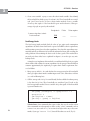
3. Besides looking at the mean or the median value of consumption, we can also easily look at the whole distribution of consumption using scatter. The following
plots the cumulative distribution function curve of per capita total expenditure.
. cumul pcexp, gen(pcexpcdf)
. twoway scatter pcexpcdf pcexp if pcexp<20000,
ytitle(“Cumulative Distribution of pcexp”) xtitle
(“Per Capita total expenditure”) title(“CDF of
Per Capita Total Expenditure”) subtitle (“Exercise
1.3”) saving (cdf1, replace)
The cumul command creates a variable called pcexpcdf that is defined as the
empirical cumulative distribution function (cdf) of pcexp; in effect, it sorts the
data by pcexp, and creates a new variable that accumulates and normalizes
pcexp, so that its maximum value is 1. To explore the variable, try
373
APPENDIX 3: Exercises
3
list
sort
list
list
pcexp pcexpcdf in 1/10
pcexp
pcexp pcexpcdf in 1/10
pcexp pcexpcdf in –10/-1
Then use the code shown here to graph the cdf. Feel free to experiment with
the scatter command. The graph is also saved in a file called cdf1.gph.
When you want to look at the graph later, just type “graph use cdf1”.
The cumulative distribution function curve of a welfare indicator can reveal
much information about poverty and inequality. For example, if we know the
value of a poverty line, we can easily find the corresponding percentage value of
people below the line. Suppose the poverty line is 5,000. Then the command
sum pcexpcdf if pcexp<5000
will give the poverty rate (under the “max” heading).
(For consideration: Why is the mean not the appropriate measure of poverty here?)
4. Keep pcfood pcexp pafood paexp famsize2 hhcode, merge with
hh.dta, sort by hhcode, and save as pce.dta in the c:\intropov\data
directory.
Household Weights
374
In most household surveys, observations are selected through a random process, but
different observations may have different probabilities of selection. Therefore, we
need to use weights that are equal to the inverse of the probability of being sampled.
A weight of wj for the jth observation means, roughly speaking, that the jth observation represents wj elements in the population from which the sample was drawn.
Omitting sampling weights in the analysis usually gives biased estimates, which may
be far from the true values (see chapter 2).
Various postsampling adjustments to the weights are sometimes necessary. A
household sampling weight is provided in the hh.dtafile. This is the right
weight to use when summarizing data that relate to households.
However, we are often interested in the individual, rather than the household, as
the unit of analysis. Consider a village with 60 households; 30 households have 5
individuals each (with income per capita of 2,100), while the other 30 households
have 10 individuals each (with income per capita of 1,200). The total population of
the village is 450. Now suppose we take a 10 percent random sample of households,
picking three 5-person households and three 10-person households. We would estimate the mean income per capita to be 1,650. While this properly reflects the nature
of households in the village, it does not give information that is representative of
APPENDIX 3: Exercises
3
individuals: the village has 150 people in 5-person households and 300 people in
10-person households. Weighted by individuals, per capita income in this village is
in fact 1,500. (Try the calculation!) Such computations can be done easily in Stata.
In estimating individual-level parameters such as per capita expenditure, we need
to transform the household sample weights into individual sample weights, using the
following Stata commands:
. gen weighti = weight*famsize
. table region [pweight=weighti], c(mean pcexp)
Stata has four types of weights: fweight, pweight, aweight, and iweight.
Of these, frequency weights and analytic weights are most important.
• Frequency weights (fweight) indicate how many observations in the population are represented by each observation in the sample. It takes integer values.
• Analytic weights (aweight) are especially useful when working with data that
contain averages (for example, average income per capita in a household). The
weighting variable is proportional to the number of persons over which the average was computed (number of members of a household, for instance). Technically, analytic weights are in inverse proportion to the variance of an observation
(that is, a higher weight means that the observation was based on more information and so is more reliable in the sense of having less variance).
Further information on weights may be obtained by typing help weight.
Now let’s repeat some previous estimations with the newly created weights:
Dhaka
Average household size
Average per capita food expenditure:
Average per capita total expenditure:
Chittagong
Khulna
Rajshahi
–———— –————––– ———— –————
–———— –————––– ———— –————
–———— –————––– ———— –————
Are the weighted averages very different from unweighted ones?
The Effects of Clustering and Stratification
If the survey under consideration has a complex sampling design, the standard errors
of estimates (and sometimes even the means) will be biased if clustering and stratification are ignored.
Consider the following typical case of a multistage stratified random sample with
clustering.
375
APPENDIX 3: Exercises
3
• First, the country is divided into regions (the strata), and a sample size is selected
for each region. Note that it is perfectly legitimate to sample some regions more
heavily than others; indeed, one would typically want to sample a sparsely populated heterogeneous region more heavily (for example, one person per 300) than
a densely populated, homogeneous region (for example, one person per 1,000).
• Within each region, communes are randomly picked, where the probability that
a commune is picked depends on the population of the commune; in this case the
commune is the primary sampling unit (the psu). One may survey households in
a cluster within the commune—for instance, picking 20 households in a single
village. Cluster sampling is widespread because it is much cheaper than taking a
simple random sample of the population. Let us assume that someone has also
computed a weight variable (wt) that represents the number of households that
each representative household “represents”; thus, the weight will be small for
oversampled areas, and larger for undersampled areas.
Stata has a very useful set of commands designed to deal with data that have been
collected from multistage and cluster sample surveys. Information must be provided
on the structure of the survey using the svyset commands. Using our example we
would have
svyset [pweight=weighti],
clear(all)
strata(region)
psu(thana)
where region is a variable that indicates the regions.1 Having set out the structure
of the survey, svymean can be used to give estimates of population means and their
correct standard errors; and svyreg can be used to perform linear regression, taking survey design into account. Other commands include svytest (to test whether
a set of coefficients are statistically significantly different from zero) and svylc (to
test linear combinations, such as the differences between the means of two variables). Repeat the exercise from “Household Weights” and compare the results.
Dhaka
Average household size
Average per capita food expenditure:
Standard deviation of per capita food
expenditure:
Average per capita total expenditure:
376
Chittagong
Khulna
Rajshahi
–———— –————––– ———— –————
–———— –————––– ———— –————
–———— –————––– ———— –————
–———— –————––– ———— –————
Are the new weighted averages, adjusted for clustering and stratification, very different from the unweighted ones?
—————————————————————————————————
—————————————————————————————————
—————————————————————————————————
APPENDIX 3: Exercises
3
Exercise 2. Chapter 3, Poverty Lines
To compare poverty measures over time, it is important that the poverty line itself
represent similar levels of well-being over time and across groups. Three methods
have been used to derive poverty lines for Bangladesh: direct caloric intake, foodenergy intake, and cost of basic needs.
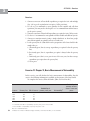
The following table gives a nutritional basket, in per capita terms, considered
minimal for the healthy survival of a typical adult in a family in rural Bangladesh.
Direct Caloric Intake
The direct caloric intake method considers any household not meeting the nutritional requirement of 2,112 Calories per day per person as poor.2 For this method,
we need to know the quantity of every food item consumed by households and its
calorie content. With that information, we calculate the total calorie content of the
food actually consumed and derive an equivalent daily caloric intake per capita for
each household. The data set c:\intropov\data\consume.dta includes the
quantity of 10 food items consumed. (“Potatoes” and “other vegetables” listed in
the table are combined into one item called “vegetables” in the survey; assume that
the total per capita daily calorie provision of this combined item is 62 and the
quantity is 177 grams.)
1. Use the quantity information from the data set and the calorie content information from the above table to calculate each household’s per capita caloric intake
(in Calories per day). (Hint: The unit in the data set is kilograms per week, and
this needs to be converted into grams per day.)
Table A3.1 Bangladesh Nutritional Basket
Per capita normative daily requirements
Food items
Calories
Rice
Wheat
Pulses
Milk (cow)
Oil (mustard)
Meat (beef)
Fish
Potatoes
Other vegetables
Sugar
Fruit
Total
1,386
139
153
39
180
14
51
26
36
82
6
2,112
Source: Wodon 1997, 93.
Quantity (gram)
397
40
40
58
20
12
48
27
150
20
20
832
Average rural consumer
price (taka/kilogram)
15.19
12.81
30.84
15.90
58.24
66.39
46.02
8.18
38.30
30.49
28.86
377
APPENDIX 3: Exercises
3
2. Create a new variable cpcap to store this caloric intake variable. Now identify
the households for which cpcap is less than 2,112. These households are considered “poor” based on the direct caloric intake method. Create a variable
directp that equals 1 if the household is poor and 0 otherwise. What percentage of people are poor by this method?
% poor using direct caloric
intake method
Bangladesh
Dhaka
Other regions
58.8
——
————
Food-Energy Intake
The food-energy intake method finds the value of per capita total consumption
expenditures at which a household can be expected to fulfill its caloric requirement,
and determines poverty based on that expenditure. Note that this expenditure automatically includes an allowance for both food and nonfood items, thus avoiding the
tricky problem of determining the basic needs for those goods. This method does
not need price data either, but as explained in chapter 3, it can also give very misleading results.
A simple way to implement this method is to rank households by their per capita
caloric intakes and calculate the mean expenditure for the group of households that
consume approximately the stipulated per capita caloric intake requirement. Proceed as follows:
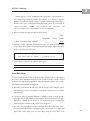
1. Merge cpcap with hh.dta and calculate the average pcexp for the households
whose per capita caloric intake is within 10 percent of 2,112, either above or below
(see code in following box).
2. Call the average value feipline and identify the households for whom pcexp
is less than feipline. These households are considered “poor” based on the
food-energy intake method. Create a variable feip that equals 1 if the household
is poor and 0 otherwise.
. sum pcexp [aw=weighti] if cpcap<2112*1.1 &
cpcap>2112*.9
. gen feipline = r(mean)
. gen feip = (pcexp <= feipline)
378
Technical note: Stata commands that report results also save the results so that
other commands can subsequently use those results; “r-class” commands, such as
summarize, save results in r() in version 6.0 or higher. After any r-class commands, if you type “return list”, Stata will list what was saved. (Try it!)
APPENDIX 3: Exercises
3
Another group—“e-class” commands such as regress—save results in e()
and estimates list will list saved results. For example, e(b) and e(V) store the
estimates of coefficients and the variance-covariance matrix, respectively. There is
an easier way to access coefficients and standard errors: either _b(varname) or
_coef(varname) contains the coefficient on varname, and
_se(varname) refers to the standard error of the coefficient.
3. What percentage of people are poor by this method?
Bangladesh
% poor using food intake method
______
Dhaka
Other
regions
_____
67.9
4. Challenge: A more sophisticated method is to regress per capita total expenditure
on per capita caloric intake and then predict the expected per capita expenditure
at the 2,112 Calorie level. Try this!
. regress pcexp cpcap [aw=weighti]
. gen feipline=_b[_cons] + _b[cpcap]*2112
5. Should there be separate regression for each region?
Cost of Basic Needs
The idea behind the cost of basic needs method is to find the value of consumption
necessary to meet minimum subsistence needs. Usually it involves a basket of food
items based on nutritional requirements and consumption patterns, and a reasonable allowance for nonfood consumption.
1. According to the basket in table A3.1 and the average rural consumer prices,
how much money does a household of four need each day to meet its caloric
requirements?
2. One way to derive the nonfood allowance is simply to assume a certain percentage of the value of minimum food consumption. How much annual total expenditure does a family of four need if it is to avoid being poor, assuming that
nonfood expenses amount to 30 percent of food expenses?
3. vprice.dta gives village-level price information on all 11 food items. Therefore, we can actually calculate a food poverty line (call it foodline) and a total
poverty line (call it cbnpline) for each village using the cost of basic needs
379
APPENDIX 3: Exercises
3
method and merge this variable with pce.dta. (Hint: Here we need to sort
both data sets and merge by thana vill.) Do this, and create a variable cbnp
that equals 1 for the poor and 0 for the nonpoor.
4. What percentage of people are poor by this method?
% poor by cost of basic needs
method
Bangladesh
Dhaka
Other
regions
________
______
______
5. The percentage of people in poverty varies according to the three methods.
Which method do you consider to be most suitable here? Why?
6. Keep all imputed poverty lines and poverty indicators, merge with pce.dta, and
save the file as final.dta.
Exercise 3. Chapter 4, Measures of Poverty
A Simple Example
In Stata, open the data file example.dta and browse the data using Stata “Data
Browser” or type in the numbers shown here. You should see a spreadsheet listing
information exactly as presented in the following table.
380
The data consist of information on consumption by all the individuals in three
countries (A, B, and C). Each country has just 10 residents.
APPENDIX 3: Exercises
3
1. Summarize the consumption level for each of the three countries:
————————————————————————————————
2. Assuming a poverty line of 125, calculate the following poverty rates for each
country:
Country
A
B
a. Using the headcount index
______
______
b. Using the poverty gap index
______
______
c. Using the squared poverty gap index
______
______
(Hint: The relevant formulas are provided in chapter 4. Try programming the
Stata rather than doing the computations by hand or using Excel.)
C
______
______
______
results in
3. Which country has the highest incidence of poverty? Justify your answer.
Poverty Measures for Rural Bangladesh 1999
Now let’s work with the per capita food expenditure and the per capita total expenditure (pcfood and pcexp in c:\intropov\data\final.dta) created in Exercise
1, and use cbnpline (the cost of basic needs poverty line derived in Exercise 2).
Technical note: Although it is possible to program the calculation of different
measures of poverty, it is simpler to use programs that have been written by others. In Stata these programs are known as.ado programs. The basic version of
Stata comes with a large library of such programs, but for specialized work (such
as computing poverty rates) it is usually necessary to install .ado programs that
have been provided on a diskette or obtained on the Web.
For computing poverty rates and their accompanying standard errors, a useful
program is FGT.ado , which is based on poverty.ado written by Philippe
Van Kerm; the standard error calculation follows Deaton (1997). The FGT.ado
file should be put in your working directory; or into a directory given by
c:\ado\plus\f (which you may need to create for this purpose). Two other
useful .ado programs are SST.ado (for computing the Sen-Shorrocks-Thon
poverty measure) and Sen.ado (for computing the Sen index of poverty).
These files are available at: http://mail.beaconhill.org/~j_haughton. Other .ado
programs are available on the Internet; for an example, and how to access them,
see “Finding and Using .ado Files” below.
FGT.ado can calculate the headcount index (or FGT(0)), the poverty gap index
(or FGT(1)), and the squared poverty gap index (or FGT(2)). For example,
. FGT y, line(1000) fgt0 fgt1 fgt2
381
APPENDIX 3: Exercises
3
will calculate the headcount ratio, the poverty gap ratio, and squared poverty gap
index using a poverty line of 1,000 and welfare indicator y. Be careful: the command
is case sensitive, and in this case FGT must be written in capital letters. After line,
the brackets must contain a number. Instead of typing all three measures, one could
specify the all option, or just some of the measures. If sd is typed, the command
will also give standard errors for the estimates, which is very useful in determining
the size of sampling error.
The command above works when there is a single poverty line. However, some
researchers prefer to compute different poverty lines for each household (as a function of household size, local price levels, and the like). Assume that these tailor-made
poverty lines are in a variable called povlines. Now the appropriate command
becomes
. FGT y, vline(povlines) fgt0 fgt1 fgt2 sd
You can specify conditions, range, and weights with these commands. For example, the following command calculates the headcount ratio for the Dhaka region
based on a poverty line of 3,000.
. FGT pcexp [aw=weighti] if region==1, line(3000)
fgt0
Sen.ado and SST.ado calculate the Sen index and the SST index, respectively.
The syntax follows the same format, but does not compute standard errors. So, for
example, one could use
. Sen y, line(1000)
. SST y, line(1000)
382
An ambitious attempt to create a suite of programs to measure poverty and
inequality within Stata has been undertaken by Abdelkrim Araar and Jean-Yves
Duclos of Université Laval. After first creating stand-alone software for measuring poverty and inequality—the DAD (Distributive Analysis/Analyse Distributive)
program—they then produced DASP: Distributive Analysis Stata Package; version 1.4
was published in December 2007, and may be downloaded from the DASP Web site
(http://132.203.59.36/DASP/dmodules/madds14.htm). DASP is an add-in to Stata;
once the program has been downloaded, every time Stata is opened it is possible to
click on the User button at the top of the screen and then to click on DASP, which in
turn provides a set of menu-driven options. In addition to basic measures of poverty
and inequality, DASP can check for dominance, decompose inequality into components, and generate the Lorenz curve and other graphs; further details are given in
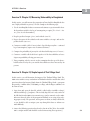
the manual (Araar and Duclos 2007). By way of illustration, here are a couple of
APPENDIX 3: Exercises
3
commands that can be used within Stata once DASP has been downloaded; the first
measures the headcount index, producing the standard error of the estimate of the
poverty rate, and lower and upper bounds of a 95 percent confidence interval, while
the second computes the Gini index of inequality, again with a standard error and
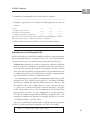
confidence interval.
Command
ifgt pcexp, alpha(0) pline(3000)
Output
Poverty index : FGT index
Sampling weight : weighti
Parameter alpha : 0.00
---------------------------------------------------------------------------Variable | Estimate
STD
LB
UB
Pov. line
----------+---------------------------------------------------------------pcexp | 0.037168 0.011489 0.014597 0.059739 3000.00
--------------------------------------------------------------------Command
igini pcexp
Output
Index : Gini index
Sampling weight : weighti
--------------------------------------------------------------------Variable
| Estimate
STD
LB
UB
------------------+------------------------------------------------1: GINI_pcexp | 0.266652 0.015956 0.235305 0.297999
--------------------------------------------------------------------Now we are ready to turn to the measurement of poverty using the data from the
Bangladesh Household and Expenditure Survey 1991/92.
1. Compute the five main measures of poverty (headcount, poverty gap, squared
poverty gap, Sen index, and Sen-Shorrocks-Thon index) for per capita expenditure, using both the food poverty line and the total poverty line derived by the
cost of basic needs method in the previous exercise.
Headcount index
Poverty gap index
Squared poverty gap index
Sen index
Sen-Shorrocks-Thon index
Food poverty line
________
________
________
________
________
Total poverty line
________
________
________
________
________
383
APPENDIX 3: Exercises
3
2. Compute the headcount and poverty gap indexes for specific subgroups using the
food poverty line.
Dhaka region
Other three regions
Households headed by men
Households headed by women
Large households (>5)
Small households ( 5)
Headcount index
________
________
________
________
________
________
Poverty gap index
________
________
________
________
________
________
3. Repeat exercise 2 above using the total poverty line.
Dhaka region
Other three regions
Households headed by men
Households headed by women
Large households (>5)
Small households (⭐5)
Headcount index
________
________
________
________
________
________
Poverty gap index
________
________
________
________
________
________
Finding and Using .ado Files
There are a wealth of .ado files on the Web, and some of them are fairly easy to
locate. For example, suppose one wants to compute the Sen index of poverty. From
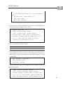
within Stata, type search Sen, which will yield the following:
384
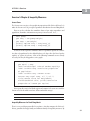
Now by double-clicking on sg108, you will obtain the following page, assuming
that your computer is connected to the Internet.
APPENDIX 3: Exercises
3
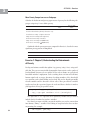
Double-click again, this time on click here to install, and the relevant
.ado file will be found, downloaded, and placed in the appropriate folder on your
computer. Once this has been done successfully, you will get a screen like this one:
This file is called poverty.ado. To find out more about it, simply type help
poverty. This program generates many measures of poverty (but not, unfortunately, their standard errors). For a sampling of the output, try
. poverty pcexp [aw=weighti], line(5000) all
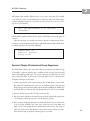
Exercise 4. Chapter 5, Poverty Indexes: Checking for Robustness
The robustness of poverty measures is important because if poverty measures are
not accurate, many conclusions about poverty comparisons between groups and
over time may not be warranted.
Sampling Error
For example, the fact that poverty calculations are based on a sample of households rather than the population implies that calculated measures carry a margin
385
APPENDIX 3: Exercises
3
of error. When the standard errors of poverty measures are large, small changes in
poverty may well be statistically insignificant and should not be interpreted for
policy purposes.
As noted above, FGT also computes the standard errors of its poverty measures if
option sd is specified:
. FGT y, line(1000) fgt0 fgt1 sd
1. Now let’s recompute the headcount index and poverty gap index for Dhaka, and
for the rest of the country, using the total poverty line, and compute the standard
errors of the two measures as well.
Dhaka region: Poverty rate
Standard error of poverty rate
Other three regions: Poverty rate
Standard error of poverty rate
Headcount index
________
________
________
________
Poverty gap index
________
________
________
________
2. Does the factor of standard errors change any conclusion about the poverty comparison between Dhaka and other regions?
Measurement Error
Another reason we need to be very careful in poverty comparisons is because the
data collected are measured incorrectly. This could be due to recall error on the part
of respondents while answering survey questions, or because of enumerator error
when entering the data into specific formats. Let us simulate measurement error in
per capita expenditure, and then investigate what effect this error has on basic poverty
measures. Try the following:
. sum pcexp [aw=weighti]
. gen mu = r(sd)*invnorm(uniform())/10
. gen pcexp_n1 = pcexp + mu
386
Here we assume that the measurement error is a random normal variable with
a standard error as big as one-tenth of the standard error of observed per capita
expenditure. Let us assume that the measurement error, mu, is additive to observed
per capita expenditure. Note that, by design, this error is independent of observed
per capita expenditure and of any other household or community characteristics.
APPENDIX 3: Exercises
3
1. Now recompute the headcount ratio and poverty gap ratio using this new per
capita expenditure.
Headcount index
Poverty gap index
pcexp
________
________
pcexp_n1
________
________
2. Are these measures different for the headcount index? For the poverty gap index?
3. Now consider the following situation. If the measurement error is correlated with
a household characteristic—for example, if subsistence farmers usually underreport their consumption of own production—will the measurement error problem be more or less severe?
Sensitivity Analysis
Apart from taking standard errors into account, it is also important to test the sensitivity of poverty measures to alternative definitions of consumption aggregates and
alternative ways of setting the poverty line. For example, some nonfood items are
excluded from the expenditure aggregate on the basis that those items are irregular
and do not reflect a household’s command over resources on average. Also, a 30 percent allowance for nonfood expenditure is arbitrary.
1. Create a new measure of total expenditure that includes the previously excluded
irregular nonfood expenditure (expnfd2), compute the three FGT poverty
measures of per capita expenditure (pcexp_n2), and compare the results with
those based on the original definition of expenditure (pcexp).
Headcount index
Poverty gap index
Squared poverty gap index
pcexp
________
________
________
pcexp_n2
________
________
________
The nonfood allowance can be estimated from data. Two methods have been considered (see chapter 4).
• The first finds the average nonfood expenditure for households whose total
expenditure is equal (or close) to the food poverty line. The nonfood expenditure
for this group of households must be necessities because the households are giving up part of minimum food consumption to buy nonfood items.
387
APPENDIX 3: Exercises
3
• The second finds the nonfood expenditure for households whose food expenditure is equal (or close) to the food poverty line.
Because the second is more generous than the first, the two are usually referred to
as the “lower” and the “upper” allowances and the poverty lines constructed using
them are called “lower” and “upper” poverty lines, respectively.
2. Try the following, then compare the results of using the two poverty lines:
. sum pcnfood [aw=weighti]
& pcfood>foodline*.9
. gen line_u = foodline +
. sum pcnfood [aw=weighti]
& pcexp>foodline*.9
. gen line_l = foodline +
Poverty line
Headcount index
Poverty gap index
if pcfood<foodline*1.1
r(mean)
if pcexp<foodline*1.1
r(mean)
lower
________
________
upper
________
________
3. Challenge: Compare poverty measures when using per-adult-equivalence scale
expenditure (paeexp), with those of using per capita expenditure.
Stochastic Dominance
One may also explore the robustness of poverty comparisons by using stochastic
dominance tests. The first-order stochastic dominance test compares the cumulative
distribution functions of per capita expenditure. Let’s compare the cumulative distributions for Dhaka with those of the rest of Bangladesh.
1. First, generate the cumulative distribution function for Dhaka region. (Note: You
may need to use the hh.dta file and merge it with the consume.dta file; you
might also need to create weighti as the product of weight and famsize.)
388
. * Note the double equal signs to represent
the identity
. keep if region == 1
. sort pcexp
. * Now create a running sum of the weighti
variable
APPENDIX 3: Exercises
3
. gen cump1 = sum(weighti)
. * This normalizes cump1 so it varies between 0
and 1
. replace cump1 = cump1/cump1[_N]
. keep cump1 pcexp
. save temp, replace
2. Now generate the cumulative distribution cump2 for the rest of Bangladesh. Keep
cump2 and pcexp, and append temp.dta by
.
.
.
.
append using temp
label variable cump1 “Dhaka”
label variable cump2 “other regions”
scatter cumpl cump2 pcexp if pcexpscatter
intcump1 intcump2 pcexp if pcexp<20000, c(l l)
m(i i) title(“CDFs for Dhaka and other
regions”) clwidth(medthick thin)
3. Does one distribution dominate another?
4. If the two lines cross at least once, then we may need to test for second-order stochastic dominance. The poverty deficit curve is the integral of the cumulative distribution up to every per capita expenditure value. After creating cump1, it may
be obtained by
. gen intcump1 = sum(cump1)
. keep intcump1 pcexp
. save temp, replace
Create intcump2 for the rest of Bangladesh. After combining variables and
labeling them properly,
. label variable intcump1 “Dhaka”
. label variable intcump2 “Other regions”
. scatter intcump1 intcump2 pcexp if pcexp<20000,
c(l l) m(i i) title(“Poverty Deficit Curves for
Dhaka and other regions”) clwidth(medthick thin)
389
APPENDIX 3: Exercises
3
5. Does one distribution dominate another here?
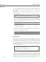
Challenge: Bootstrapping Standard Error for the SST Index
The bootstrapping technique can be used to calculate standard errors of poverty
measures, and is especially helpful in cases where the standard errors are impossible
to solve analytically (for example, with the SST index of poverty). The idea is quite
simple. Repeat the calculation of the poverty measure many times, each time using a
new random sample drawn from the original one with replacement. For this purpose, it is necessary to use macros and loops in Stata. The following code is an example; it could be copied or typed into the do-file editor and executed.
set more 1
local i = 1
while ‘i’<=100 {
use c:\intropov\data\final.dta, clear
keep pcexp weighti cbnpline
bsample _N
SST pcexp [aw=weighti], line(5000)
drop _all
set obs 1
gen sst = $S_6
if ‘i’ ==1 {
save temp, replace
}
else {
append using temp
save temp, replace
}
local i = ‘i’ + 1
}
sum sst
The code above repeats the calculation of the SST index 100 times; the sum command provides the standard error of these 100 estimates.
390
APPENDIX 3: Exercises
3
Exercise 5. Chapter 6, Inequality Measures
Lorenz Curve
The Lorenz curve can give a clear graphic interpretation of the Gini coefficient. Let’s
make the Lorenz curve of per capita expenditure distribution for rural Bangladesh.
First, we need to calculate the cumulative shares of per capita expenditure and
population: (Reminder: information on pcexp is in consume.dta.)
.
.
.
.
.
sort pcexp
gen cumy = sum(pcexp*weight)
gen cump = sum(weight)
quietly replace cumy = cumy/cumy[_N]
quietly replace cump = cump/cump[_N]
Second, we need to plot the cumulative share of expenditure against the cumulative share of population. It is also helpful to have a 45-degree line (the line of perfect
equality) as a point of reference. Some of the following commands are not strictly
necessary, but they do help produce a nice graph.
.
.
.
.
sort pcexp
gen equal = cump
label variable equal “Line of Perfect Equality”
label variable cump “Cumulative proportion
of population”
. label variable cumy “Lorenz curve”
. scatter cumy equal cump, c(l l) m(i i)
title(“Lorenz Curve for Bangladesh”)
clwidth(medthick thin) ytitle(“Cumulative
proportion of income per capita”)
Now repeat this exercise for Dhaka region and compare its Lorenz curve with the
Lorenz curve for the whole rural area. What conclusions emerge?
Inequality Measures for Rural Bangladesh
There is a very useful program called ineqdeco.ado that computes the Gini coefficient, generalized entropy family, and Atkinson family of inequality measures. By
391
APPENDIX 3: Exercises
3
typing search ineqdeco within Stata and following the instructions it is straightforward to load this .ado file onto your computer. As in Exercise 3, you can use these
programs just like other Stata commands. The syntax is
. ineqdeco y [if...][w=weight], [by(...)]
When the by option is used, this program decomposes inequality into the withingroup and between-group components, which is often very helpful. Here is a more
concrete example of the command at work:
. ineqdeco rlpcex1 [w=hhsizewt], by(urban98)
In this example, we get several measures of inequality for real per capita expenditure (rlpcex1), adjusted for weights (given by hhsizewt), and separated into
urban and rural components.
Another helpful program is fastgini, which calculates the Gini coefficient
along with jackknife standard errors. For example, the command fastgini
rlpcex1 [w=hhsizewt], jk would generate the Gini coefficient and its standard
error for real per capita expenditure rlpcex1.
Let’s continue using per capita total expenditure to calculate inequality measures:
1. Compute the Gini coefficient, the Theil index, and the Atkinson index with
inequality aversion parameter equal to 1 for the four regions.
All regions
Dhaka region
Other three regions
Gini
Theil
Atkinson
________
________
________
________
________
________
________
________
________
2. Now repeat the above exercise using decile dispersion ratios, and the share of consumption of the poorest 25 percent. Stata command xtile is good for dividing
the sample by ranking. For example, to calculate the consumption expenditure
ratio between the richest 20 percent and the poorest 20 percent, you need to identify those two groups.
. xtile group = y, nq(5)
392
The command xtile will generate a new variable group that splits the sample
into five groups according to the ranking of y (from smallest to largest, that is,
the poorest 20 percent will have group==1, while the richest 20 percent will
have group==5). Similarly, to identify the poorest 25 percent, you need to split
the sample into four groups.
APPENDIX 3: Exercises
3
top 20%
÷ bottom 20%
top 10%
÷ bottom 10%
Percentage of
consumption of
poorest 25%
All Bangladesh
________
________
________
Dhaka region
Other regions of
Bangladesh
________
________
________
________
________
________
3. Challenge: Many inequality indexes can be decomposed by subgroups. Decompose the Theil index by region and comment on the results.
Exercise 6. Chapter 7, Describing Poverty: Poverty Profiles
In the previous exercises we computed poverty measures for various subgroups, such
as regions, gender of head of household, household size, and so on. Another way to
present a poverty profile is by comparing the characteristics of the “poor” with those
of the “nonpoor.”
Characteristics of the Poor
Complete the following table, where “poor” and “nonpoor” are defined by cbnp in
Exercise 2.
poor
% of all households
% of total population
Average distance to paved road
Average distance to nearest bank
% of households with electricity
% of households with a sanitary toilet
Average household assets (taka)
Average household land holding (decimals)
______
______
______
______
______
______
______
______
[Reminder: a decimal is 0.01 of an acre.]
Average household size
% of households headed by men
Average schooling of head of household (years)
Average age of head (years)
Average head of household working hours on
nonfarm activities (per year)
______
______
______
______
______
nonpoor
______
______
______
______
______
______
______
______
______
______
______
______
______
393
APPENDIX 3: Exercises
3
More Poverty Comparisons across Subgroups
Calculate the headcount and poverty gap measures of poverty for the following subgroups, using cbnpline to define poverty.
Headcount
index
Poverty gap
index
Household head has no education
Household head has a primary education only
Head had secondary or higher education
Large land ownership (>0.5 ha/person)
Small land ownership or landless
Large asset ownership (>50,000 taka)
Small asset ownership ( 50,000 taka)
Combined with the poverty measures computed in Exercise 3, describe the most
significant poverty patterns in Bangladesh.
Exercise 7. Chapter 8, Understanding the Determinants
of Poverty
Develop and estimate a model that explains log(pcexp/cbnpline) using available data. The regressors may include demographic characteristics such as gender of
head and family structure; access to public services such as distance to a paved road;
household members’ employment such as working hours on farm and off farm;
human capital such as average education of working members of the household;
asset positions such as land holding; and so forth. You need to identify potentially
relevant variables and the direction of their effect. Then put all those variables
together and run the regression. Report the result and discuss whether it matches
your hypothesis. If not, give possible reasons.
. gen y = log(pcexp/cbnpline)
. reg y age age2 workhour x1-x3 [aw=weighti]
The expression x1-x3 represents other explanatory variables that you want to
include; don’t feel confined to just three variables!
Note that if you want to include categorical variables, you need to convert them
into dummy (“binary”) variables if the ranking of categorical values does not have
any meaning. For example,
394
. tab region, gen(reg)
APPENDIX 3: Exercises
3
will generate four variables, labeled reg1, reg2, reg3, and reg4. The variable
reg1 takes on a value of 1 for Dhaka and zero otherwise, and so on. When using a
set of such dummy variables in a regression, one must be left out, to serve as a reference area. So, for instance,
. reg y age age2 workhour x1-x3 reg2-reg4
[aw=weighti]
would include dummy variables for the regions, with Dhaka serving as the point of
reference.
After the regression, it is usually a good idea to plot the residuals against the fitted values to ensure that the pattern appears sufficiently random. This could be done
by adding, right after the regression command,
. predict yhat, xb
. predict e, residuals
. scatter e yhat
Exercise 8. Chapter 10, International Poverty Comparisons
The World Bank estimates the extent and evolution of world poverty with the help
of PovcalNet, a software interface that is available on line at http://iresearch.world
bank.org/PovcalNet/jsp/index.jsp. This exercise represents an exploration of world
poverty using PovcalNet. To answer this exercise you will need to use a browser such
as Explorer and log in to PovcalNet.
1. Assume a poverty line of $1.25 per person per day (in 2005 prices). Create a table
that shows the headcount poverty rate for the six main regions (East Asia and
Pacific, Europe and Central Asia, Latin America and the Caribbean, the Middle East
and North Africa, South Asia, and Sub-Saharan Africa) for 1981, 1993, and 2005.
2. Repeat 1, but for a poverty line of $2 per person per day.
3. Based on 1 and 2, which are the world’s poorest regions? And which regions have
seen the biggest reduction in poverty over the past two decades?
4. Pick a country. Graph the evolution of its headcount poverty rate over time (that
is, for every year available: 1981, 1984, 1987, 1990, 1993, 1996, 1999, 2002, and
2005). On the same graph, show the headcount poverty rate for the region in
which the country is located. Relative to the region, has the country you chose
done relatively well, or poorly, in reducing poverty over time?
395
APPENDIX 3: Exercises
3
5. Pick any two countries. Compute the headcount poverty rate for each country at
a dozen different poverty lines ($1.00 a day, $1.25 a day, $1.50 a day, and so on)
and graph these curves. The horizontal axis will show the poverty line and the
vertical axis will show the headcount poverty rate. These are poverty incidence
curves. Which country has the higher poverty rate? Explain
Exercise 9. Chapter 11, Panel Data
The goal in this exercise is to create a panel of data. The Bangladeshi data come from
a panel of households surveyed in 1991 and 1998. The relevant data are hh91.dta,
hh98.dta, etc. (or hh91v7s.dta, and so on, if one is using Stata version 7). Each household has a single id called nh (“number of household”).
1. Download the household data for 1998 and rename the variables (except for nh).
For instance:
rename sexhead sexhead98
This is done so that when the data from the two surveys are merged, it will still be
possible to distinguish the 1998 numbers from the 1991 numbers.
2. Sort the file using nh and save it with a name like hh98newlabels.dta.
3. Now open the household data file for 1991, sort it by nh, and merge it with
hh98newlabels.dta.
4. Check that the villages are comparable (for example, using compare vill
vill98).
5. Use a paired t-test to determine whether there was a significant change in the
education level of heads of household between 1991 and 1998. Do the same for
land holdings and access to toilets.
6. Repeat step 5, but use an unpaired t-test.
Exercise 10. Chapter 11, Transition Matrix
In this exercise, you will create a transition matrix that shows the extent to which
households moved into or out of poverty.
1. Open consume98.dta, rename the expenditures by suffixing 98. Merge with consume91.dta (using nh to link the files). Save as consume9198.dta.
396
2. Create poverty lines for 1991 and 1998 using the vprice91.dta and vprice98.dta
files, as set out in the Exercise 2 for chapter 3. Food needs are as shown in
APPENDIX 3: Exercises
3
table A3.1; assume the cost of basic needs poverty line is the food poverty line
times 1.3. Call the poverty lines foodline91, cbnpline91, foodline98, and
cbnpline98. Merge this information using thana and vill to create a single file
with all the poverty lines. Call it povlines91and98.dta.
Remember: gen fpovline = pveg*3.4 + pfish*8.7 + ...
gen cbnpline = 1.3*fpovline
3. Construct a poverty indicator (1=poor) for 1991 and for 1998, and show the
poverty transition matrix—that is, a simple table showing who was poor in both
years, in neither year, in 1991 only, or in 1998 only.
Exercise 11. Chapter 11, Quintile Transition Matrix
In this exercise, you will construct a quintile transition matrix and generate measures
of chronic, persistent, and transient poverty using data from Bangladesh.
Preparatory Steps
1. Open consume98.dta, keep nh hhexpfd hhexpnfd and hhexpnfd2, rename
each of these by appending 98, sort by nh, and save under a new name such as
rconsume98.dta.
2. Open consume91.dta, keep the same variables, sort by nh, merge with rconsume98, check that the merge has worked (using tab _merge), drop the
_merge variable, sort by nh, and save as rconsume9198.dta.
3. If you have not already done so, open hh98big7bs.dta and rename each variable
(except nh) by suffixing 98. For example:
rename vill vill98.
This file has information on income. Sort using nh and save under a new name
such as revhh98.dta.
4. Now open hh91.dta, sort by nh, and merge using revhh98.dta. As usual, check that
the two files have merged, by examining _merge, and then delete this variable.
5. Sort by nh and merge using rconsume9198.dta. Save this file, which is the file
with which you will now work.
Note that prices in 1998 were 47 percent higher than in 1991, so before incomes
or expenditures can be compared, they must be adjusted for the price difference. We
will do this in the following exercises.
397
APPENDIX 3: Exercises
3
Exercises
1. Construct a measure of household expenditure per capita for 1991 and multiply
it by 1.47 to get the equivalent in 1998 prices. Call it pce91in98.
2. Use the xtile command to create quintiles for this variable and call them
qex91in98. [You may need to look up the xtile command from within Stata to
get the precise syntax.]
3. Construct a measure of household expenditure per capita for 1998. Call it pce98.
4. Use the xtile command to create quintiles for this variable and call them qex98.
5. Construct a transition matrix (using a simple tabulation) to show how people
moved from quintile to quintile between 1991 and 1998.
6. Let the poverty line be 5,500. Work out the proportions of the households in the
sample who are
a. Chronically poor (that is, average expenditure per capita is below the poverty
line)
b. Persistently poor (that is, expenditure per capita is always below the poverty
line)
c. Transiently poor (that is, were poor in one of the two years, but have average
expenditure per capita above the poverty line)
d. Never poor.
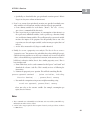
Exercise 12. Chapter 12, Basic Measurement of Vulnerability
In this exercise, you will calculate the basic measurement of vulnerability. For this
exercise, the following information is available on the income of five households.
To complete this exercise, fill in the blanks. [Hint: Use Excel for this.]
Income
100
120
130
160
220
Poverty line
125
125
125
125
125
Probability of
SD of income poverty next year
Vulnerabilitya
10
12
22
20
30
• Highly vulnerable: 1. If probability of poverty next year is >0.5.
• Somewhat vulnerable: 2. If probability of poverty next year is > P0 but <=0.5
• Not vulnerable: 3. If probability of poverty next year is <=P0.
Note: SD = standard deviation.
398
a. Indicate here whether individual is highly vulnerable, somewhat vulnerable, or not vulnerable.
Probability of
poverty at least
once in next two
years
APPENDIX 3: Exercises
3
Exercise 13. Chapter 12, Measuring Vulnerability in Bangladesh
In this exercise, you will measure the proportion of households in Bangladesh who
were “highly vulnerable to poverty” in 1998. Complete the following steps:
1. Use the 1998 Bangladesh data to construct and estimate a regression model where
the dependent variable is the log of consumption per capita. [Use final.dta
or pce.dta for the numbers.]
2. Keep the predicted output (yhat) and residuals (resid).
3. Regress the square of the residuals on the same variables as in step 1 and save the
predicted value (estvar).
4. Construct a variable (call it flessc) that is (log of food poverty line – estimated
log of consumption)/(square root of estimated variance).
5. Compute the probability of poverty for each household using norm(flessc).
6. Construct a variable called vul1 that is equal to 1 if the household has at least a
50 percent probability of being poor next year.
7. Time permitting, redo the exercise on the assumption that the age of the household head has risen by five years and the household assets have increased by 20
percent.
Exercise 14. Chapter 13, Simple Impact of Thai Village Fund
In this exercise, you will determine the impact of the Thailand Village Fund. The
2004 socioeconomic survey undertaken in Thailand included a module that asked
questions about who borrowed funds from the Thailand Village Fund—a program
that provides 1 million baht (US$25,000) per village, which villagers administer in
the form of loans.
1. Open Stata and open the data file, which is called tvf.dta (available at http://
mail.beaconhill.org/~j_haughton). This is a fairly large file, but is only a subset of
the full data from the 2004 socioeconomic survey (and so cannot be used to make
inferences about the effect of the program in Thailand; we are using it for teaching purposes only). The questions, and responses to them, are fairly well labeled,
so you should be able to navigate your way through this data set without too
much difficulty.
2. Answer the following questions based on the data in tvf.dta. [Note: the variable
a30 is a weight variable and should be used when answering these questions.]
399
APPENDIX 3: Exercises
3
a.
b.
c.
d.
e.
f.
g.
What proportion of households participated as borrowers?
Why reasons did people give for not participating? In what proportions?
How large was the average loan requested? Received?
What interest rates were charged?
For what purposes did people say they used the loans?
What was the default rate on the loans?
What fraction of borrowers had to borrow money from elsewhere in order to
repay their Village Fund loan?
h. How did the Village Fund affect households “economic situation”?
i. What changes would households like to see in the Village Fund? Distinguish
between the responses of participants and nonparticipants. Summarize the data.
3. How would you evaluate the impact of the Village Fund? Write a 200-word
proposal. [This may seem like a narrow question, but it is really asking you to
think about how you might go about measuring the impact of any program
or project.]
Exercise 15. Chapter 13, Impact of Agricultural Extension
In this exercise, you will determine the impact of agricultural extension. Download
hh98big7bs.dta. This file has familiar data from Bangladesh, but we have now
added a new variable called agextend that indicates whether a household was chosen to participate in a program of agricultural extension that provides advice and support. [Note: The variable is invented, but the rest of the data set is real.] We now want
to ask a basic question: what was the impact of the agricultural extension program?
1. First, let us look at the raw numbers.
a. Load hh98big7bs.dta, sort by the variable nh, and save.
b. Now load consume98v72.dta (or equivalent), sort by nh, and merge nh
using hh98big7bs.
c. Check that the merge worked correctly by looking at the _merge variable.
2. Now compare income and consumption levels for households that did, and did
not, get agricultural extension help.
a. Hint 1. First create measures of total income per capita, and total consumption
per capita.
b. Hint 2. Sort by agextend and then use the syntax by agextend: sum hh*
or equivalent.
400
APPENDIX 3: Exercises
3
c. Specifically, are households that got agricultural extension poorer? Richer?
Larger? Are they more reliant on farm income?
3. Next, let us assume that agricultural extension was provided randomly, once
other variables are held constant, and then ask what effect the program had.
a. Create dummy variables for each district (“thana”). The tab thana,
gen(than) command will do this nicely.
b. Run a regression of per capita income (or consumption or farm income) on
the agextend, individual variables (such as gender, age, education, family
size), and district dummy variables. The coefficient on the agextend variable
measures the impact of the program. You will probably want to run a few
regressions, one for each output variable (such as income per capita) that is of
interest.
c. Are the effects measured in 3(b) larger or smaller than in 2?
4. Finally, let us run a propensity score analysis. The idea is first to create a
“propensity score” that measures the probability that a household will get agricultural extension; and then to use this score to match each “treated” household
(that is, a household that gets agricultural extension) with an untreated household that is otherwise similar (that is, has a similar propensity score). Here is
how it might work:
a. From within Stata, use the search command to find “pscore” and “attnd” and
download the relevant *.ado files. This is mainly an issue of following the
instructions.
b. Estimate the propensity score equation. This will look something like this:
pscore agextend sexhead ... [other variables, including
district dummies] ... , pscore(fhat1) comsup
c. Now make the comparison, using nearest-neighbor matching, using
attnd xxx agextend, pscore(fhat1) comsup
where xxx refers to the outcome variable (for example, consumption per
capita) that is of interest.
Notes
1. These commands were substantially revised in Stata version 8, and the syntax differs significantly from earlier versions of Stata.
2. A calorie is the energy required to heat one gram of water by one degree Celsius. A Calorie
is 1,000 calories.
401
APPENDIX 3: Exercises
3
References
Araar, Abdelkrim, and Jean-Yves Duclos. 2007. USER MANUAL: DASP version 1.4. Université
Laval, PEP, CIRPÉE, and World Bank. [DASP stands for Distributive Analysis Stata Package.]
Deaton, Angus. 1997. The Analysis of Household Surveys: A Microeconometric Approach to
Development Policy. Baltimore, MD: Johns Hopkins University Press for the World Bank.
Wodon, Quentin T. 1997. “Food Energy Intake and Cost of Basic Needs: Measuring Poverty in
Bangladesh.” Journal of Development Studies 34 (2): 66–101.
402