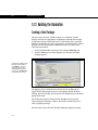
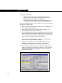
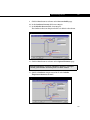
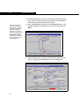
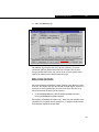
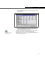
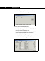
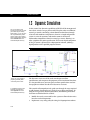
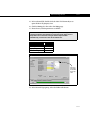
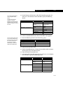
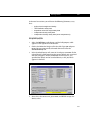
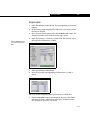
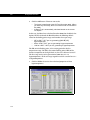
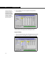
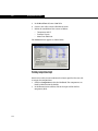
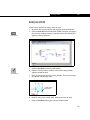
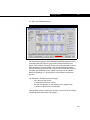
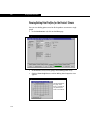
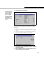
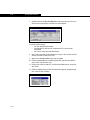
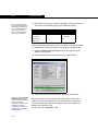
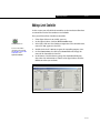
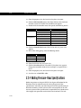
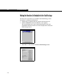
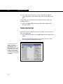
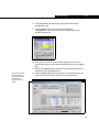
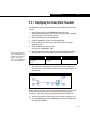
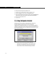
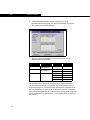
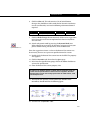
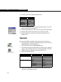
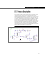
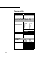
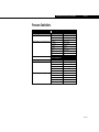
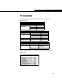
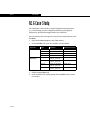
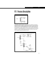
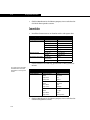
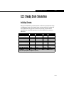
1
Copyright Notice
© 2002 Hyprotech, a subsidiary of Aspen Technology, Inc. All rights reserved.
Hyprotech is the owner of, and have vested in them, the copyright and all other intellectual property rights
of a similar nature relating to their software, which includes, but is not limited to, their computer programs,
user manuals and all associated documentation, whether in printed or electronic form (the “Software”),
which is supplied by us or our subsidiaries to our respective customers. No copying or reproduction of the
Software shall be permitted without prior written consent of Aspen Technology, Inc., Ten Canal Park,
Cambridge, MA 02141, U.S.A., save to the extent permitted by law.
Hyprotech reserves the right to make changes to this document or its associated computer program
without obligation to notify any person or organization. Companies, names, and data used in examples
herein are fictitious unless otherwise stated.
Hyprotech does not make any representations regarding the use, or the results of use, of the Software, in
terms of correctness or otherwise. The entire risk as to the results and performance of the Software is
assumed by the user.
HYSYS, HYSIM, HTFS, DISTIL, HX-NET, and HYPROP III are registered trademarks of Hyprotech.
PIPESYS is a trademark of Neotechnology Consultants.
Microsoft Windows, Windows 95/98, Windows NT, Windows 2000, Visual Basic, and Excel are registered
trademarks of the Microsoft Corporation.
Documentation Credits
Authors of the current release, listed in order of historical start on project (2002-1995):
Pamela Smith; Clement Ng, BASc; Sandy Brar, BSc; Jessie Channey, BAC; Tsitsi Ettienne, BSc; Angeline Teh,
BSc; Sarah-Jane Brenner, BASc; Conrad Gierer, BASc; Chris Strashok, BSc; Adeel Jamil, BSc; Yannick
Sternon, BIng; Nana Nguyen, BSc; Allan Chau, BSc; Muhammad Sachedina, BASc; Lisa Hugo, BSc, BA; Chris
Lowe, PEng; Kevin Hanson, PEng.
Since software is always a work in progress, any version, while representing a milestone, is nevertheless but
a point in a continuum. Those individuals whose contributions created the foundation upon which this
work is built have not been forgotten. The current authors would like to thank the previous contributors. A
special thanks is also extended by the authors to everyone who contributed through countless hours of
proof-reading and testing.
Contacting Hyprotech
Hyprotech can be conveniently accessed via the following:
Web site:
Information and Sales:
Documentation:
Training:
Technical Support:
www.hyprotech.com
[email protected]
[email protected]
[email protected]
[email protected]
Detailed information on accessing Hyprotech Technical Support can be found in the Technical Support
section of the Get Started manual.
TAH3.1-B4814-NOV02-O
Table of Contents
A
HYSYS Tutorials.........................................................A-1
1
Gas Processing Tutorial............................................. 1-1
2
3
B
1.1
Introduction .......................................................................1-3
1.2
Steady State Simulation....................................................1-4
1.3
Dynamic Simulation ........................................................1-98
Refining Tutorial......................................................... 2-1
2.1
Introduction .......................................................................2-3
2.2
Steady State Simulation....................................................2-5
2.3
Dynamic Simulation ......................................................2-114
Chemicals Tutorial ..................................................... 3-1
3.1
Introduction .......................................................................3-3
3.2
Steady State Simulation....................................................3-4
3.3
Dynamic Simulation ........................................................3-76
HYSYS Applications ...................................................B-1
G1 Acid Gas Sweetening with DEA .............................. G1-1
G1.1
Process Description ....................................................... G1-3
G1.2
Setup.............................................................................. G1-5
G1.3
Steady State Simulation................................................. G1-5
G1.4
Simulation Analysis...................................................... G1-15
G1.5
Calculating Lean & Rich Loadings ............................... G1-15
G1.6
Dynamic Simulation ..................................................... G1-17
G1.7
References................................................................... G1-34
iii
R1 Atmospheric Crude Tower .......................................R1-1
R1.1
Process Description ....................................................... R1-3
R1.2
Setup.............................................................................. R1-6
R1.3
Steady State Simulation............................................... R1-10
R1.4
Results ......................................................................... R1-18
R2 Sour Water Stripper..................................................R2-1
R2.1
Process Description ....................................................... R2-3
R2.2
Introduction .................................................................... R2-4
R2.3
Setup.............................................................................. R2-4
R2.4
Steady State Simulation................................................. R2-5
R2.5
Results ........................................................................... R2-8
R2.6
Case Study .................................................................. R2-10
P1 Propylene/Propane Splitter ......................................P1-1
P1.1
Process Description ....................................................... P1-3
P1.2
Setup.............................................................................. P1-4
P1.3
Steady State Simulation................................................. P1-5
P1.4
Results ......................................................................... P1-10
C1 Ethanol Plant ............................................................C1-1
C1.1
Process Description ....................................................... C1-3
C1.2
Setup.............................................................................. C1-6
C1.3
Steady State Simulation................................................. C1-6
C1.4
Results ......................................................................... C1-13
C2 Synthesis Gas Production........................................C2-1
C2.1
Process Description ....................................................... C2-3
C2.2
Setup.............................................................................. C2-4
C2.3
Steady State Simulation................................................. C2-9
C2.4
Results ......................................................................... C2-16
X1 Case Linking.............................................................X1-1
iv
X1.1
Process Description ....................................................... X1-3
X1.2
Building Flowsheet 1...................................................... X1-4
X1.3
Building Flowsheet 2...................................................... X1-8
X1.4
Creating a User Unit Operation.................................... X1-10
HYSYS Tutorials
A-1
A HYSYS Tutorials
The Tutorials section of this manual presents you with independent
tutorial sessions. Each tutorial guides you step-by-step through the
complete construction of a HYSYS simulation. The tutorial(s) you
choose to work through will likely depend on the simulation topic that is
most closely related to your work, your familiarity with HYSYS and the
types of simulation cases you anticipate on creating in the future.
All completed Tutorial cases
are included with your HYSYS
package, and are available on
HYSYS\Samples.
Regardless of which tutorial you work through first, you will gain the
same basic understanding of the steps and tools used to build a HYSYS
simulation. After building one of these tutorial cases, you might choose
to build one or several more, or begin creating your own simulations.
If you are new to HYSYS, it is recommended that you begin with the
steady state tutorials. These tutorials explicitly detail each step required
to complete the simulation. In steps where more than one method is
available to complete a particular action, all methods are outlined. The
dynamic tutorials (which are continued after the steady state section)
are also presented in a step-by-step manner, but are less detailed in
their explanations. They assume a rudimentary knowledge of the HYSYS
interface and methods.
The three tutorials are grouped in three general areas of interest:
1.
Gas Processing
2.
Refining
3.
Chemicals
Each area has an associated steady state and dynamic tutorial. The
dynamic tutorials use the steady state cases and add control schemes
and dynamic specifications required to run the case in Dynamic mode.
If you are interested only in steady state simulation, go through the
steady state tutorial(s) that most interest you and stop at the dynamics
section. If you are interested only in learning to apply dynamic
simulation methods, use the pre-built steady state base case, included
with HYSYS, as the starting point for your dynamic tutorial case.
A-1
A-2
Introduction
There are also several
HYSYS training courses
available. Contact your
Hyprotech agent for more
information, or visit the
training page of our web site
www.hyprotech.com.
In the chapters that follow, example problems are used to illustrate
some of the basic concepts of building a simulation in HYSYS. Three
complete tutorials are presented:
1.
The solved steady state
cases are saved in the
HYSYS\Samples folder as
TUTOR1.hsc, TUTOR2.hsc,
and TUTOR3.hsc files.
For the dynamics tutorials,
you can use the pre-built
steady state cases as your
starting point. The solved
dynamics cases are also
included as dyntut1.hsc,
dyntut2.hsc, and
dyntut3.hsc.
2.
Gas Processing
• Steady State. Models a sweet gas refrigeration plant consisting
of an inlet separator, gas/gas heat exchanger, chiller, lowtemperature separator and de-propanizer column.
• Dynamics. Models the Gas Processing tutorial case in Dynamic
mode. This tutorial makes use of the recommendations of the
Dynamic Assistant when building the case.
Refining
•
3.
Steady State. Models a crude oil processing facility consisting of
a pre-flash drum, crude furnace and an atmospheric crude
column.
• Dynamics. Models the Refining example problem in Dynamic
mode.
Chemicals
•
•
Steady State. Models a propylene glycol production process
consisting of a continuously-stirred-tank reactor and a distillation
tower.
Dynamics. Models the Chemicals example problem in Dynamic
mode. This tutorial make use of the recommendations of the
Dynamic Assistant when building the case.
Each of these tutorials will guide you step-by-step through the complete
construction of a HYSYS simulation. The tutorial you choose first will
likely depend on which one is most closely related to your work, or that
you feel most comfortable with.
Regardless of the tutorial you work through first, you will gain the same
basic understanding of the steps and tools used to build a HYSYS
simulation. Each example contains detailed instructions for choosing a
property package and components, installing and defining streams, unit
operations and columns, and using various aspects of the HYSYS
interface to examine the results while you are creating the simulation. If
you are new to HYSYS, it is recommended that you begin with one of
these tutorials in order to familiarize yourself with the initial steps
required to build a HYSYS simulation.
Often in HYSYS, more than one method exists for performing a task or
executing a command. Many times you can use the keyboard, the
A-2
HYSYS Tutorials
A-3
mouse, or a combination of both to achieve the same result. The steady
state tutorials attempt to illustrate HYSYS' flexibility by showing you as
many of these alternative methods as possible. You can then choose
which approach is most appropriate for you.
The dynamics tutorials use the steady state solution as a basis for
building the dynamic case. If you like, you can build the steady state
case and then proceed with the dynamic solution, or you can simply call
up the steady state case from disk and begin the dynamic modeling.
Starting HYSYS
With Windows NT 4.0 or Windows 95/98, the installation process creates
a shortcut to HYSYS:
HYSYS Icon
1.
Click on the Start menu.
2.
Move from Programs to Hyprotech to HYSYS.
3.
Select HYSYS.
The HYSYS Desktop appears:
Figure A.1
Menu Bar
Tool Bar
Status Bar
Object Status
Window
Maximize icon
Trace Window
Performance
Slider
To learn more about the basics of the HYSYS interface, see Chapter 1 Interface in the User Guide.
A-3
A-4
Get Started
The tutorials start in Steady
State mode, and end in
Dynamic mode.
Once you have completed one
or more tutorials, you may
want to examine the
Applications section for other
examples that may be of
interest.
You are now ready to begin building a HYSYS simulation, so proceed to
the Tutorial of your choice.
Samples Case Name
Tutorial
Chapter
Gas Processing
Chapter 1
TUTOR1.HSC
Refining
Chapter 2
TUTOR2.HSC
Chemicals
Chapter 3
TUTOR3.HSC
(Steady State/Dynamic)
dyntut1.hsc
dyntut2.hsc
dyntut3.hsc
A-4
Gas Processing Tutorial
1-1
1 Gas Processing Tutorial
1.1 Introduction......................................................................................3
1.2 Steady State Simulation ..................................................................4
1.2.1 Process Description .................................................................4
1.2.2 Setting Your Session Preferences ............................................6
1.2.3 Building the Simulation...........................................................10
1.2.4 Entering the Simulation Environment .....................................18
1.2.5 Using the Workbook ...............................................................20
1.2.6 Installing Unit Operations .......................................................34
1.2.7 Using Workbook Features ......................................................45
1.2.8 Using the PFD ........................................................................49
1.2.9 Viewing and Analyzing Results ..............................................76
1.2.10 Optional Study......................................................................87
1.3 Dynamic Simulation ......................................................................98
1.3.1
1.3.2
1.3.3
1.3.4
Modifying the Steady State Flowsheet ...................................99
Column Sizing ......................................................................107
Using the Dynamics Assistant..............................................113
Adding Controller Operations ...............................................119
1-1
1-2
1-2
Gas Processing
Gas Processing Tutorial
1-3
1.1 Introduction
The simulation will be built using these basic steps:
A solved case is located in the
file TUTOR1.HSC in your
HYSYS\Samples directory.
1.
Create a unit set.
2.
Choose a property package.
3.
Select the components.
4.
Create and specify the feed streams.
5.
Install and define the unit operations prior to the column.
6.
Install and define the column.
In this Tutorial, a natural gas stream containing N2, CO2, and C1
through nC4 is processed in a refrigeration system to remove the
heavier hydrocarbons. The lean, dry gas produced will meet a pipeline
hydrocarbon dew point specification. The liquids removed from the rich
gas are processed in a depropanizer column, yielding a liquid product
with a specified propane content. A flowsheet for this process is shown
below.
Figure 1.1
The following pages will guide you through building a HYSYS case to
illustrate the complete construction of the simulation, from selecting a
property package and components to examining the final results. The
tools available in HYSYS interface will be utilized to illustrate the
flexibility available to you.
Before proceeding, you should have read the introductory chapter which
precedes the Tutorials in this manual.
1-3
1-4
Steady State Simulation
1.2 Steady State Simulation
1.2.1 Process Description
This tutorial will model a natural gas processing facility that uses
propane refrigeration to condense liquids from the feed and a
distillation tower to process the liquids. The flowsheet for this process
appears below.
Figure 1.2
The combined feed stream enters an inlet separator, which removes the
free liquids. Overhead gas from the Separator is fed to the gas/gas
exchanger, where it is pre-cooled by already refrigerated gas. The cooled
gas is then fed to the chiller, where further cooling is accomplished
through exchange with evaporating propane (represented by the
C3Duty stream). In the chiller, which will be modeled simply as a Cooler,
enough heavier hydrocarbons condense such that the eventual sales gas
meets a pipeline dew point specification. The cold stream is then
separated in a low-temperature separator (LTS). The dry, cold gas is fed
to the gas/gas exchanger and then to sales, while the condensed liquids
are mixed with free liquids from the inlet separator. These liquids are
processed in a depropanizer column to produce a low-propane-content
bottoms product.
1-4
Gas Processing Tutorial
1-5
Once the results for the simulation have been obtained, you will have a
good understanding of the basic tools used to build a HYSYS simulation
case. At that point, you can either proceed with the Optional Study
presented at the end of the tutorial or begin building your own
simulations.
In this tutorial, three logical operations will be installed in order to
perform certain functions that cannot be handled by standard physical
unit operations:
Logical
Flowsheet Function
Balance
To duplicate the composition of the SalesGas stream in
order to calculate its dew point temperature at pipeline
specification pressure.
Adjust
To determine the required LTS temperature which gives
a specified SalesGas dew point.
HYSYS Spreadsheet
To calculate the SalesGas net heating value.
The Balance operation will be installed in the main example. In the
Optional Study section, the Adjust and Spreadsheet operations will be
installed to investigate the effect of the LTS temperature on the sales gas
heating value.
The two primary building tools, the Workbook and the PFD, will be used
to install the streams and operations and to examine the results while
progressing through the simulation. Both of these tools provide you with
a lot of flexibility in building your simulation and in quickly accessing
the information you need.
The Workbook will be used to build the first part of the flowsheet,
starting with the feed streams and building up to and including the gas/
gas heat exchanger. The PFD will be used to install the remaining
operations, from the chiller through to the column.
1-5
1-6
Steady State Simulation
1.2.2 Setting Your Session Preferences
All commands accessed via
the toolbar are also available
as menu items.
1.
To start a new simulation case, do one of the following:
• From the File menu, select New Case.
• Click the New Case icon.
The Simulation Basis Manager appears:
New Case icon
Figure 1.3
The Simulation Basis
Manager allows you to create,
modify, and manipulate fluid
packages in your simulation
case. Most of the time, as with
this example, you will require
only one fluid package for your
entire simulation.
Next, you will set your Session Preferences before building a case.
1-6
Gas Processing Tutorial
2.
1-7
From the Tools menu, select Preferences. The Session Preferences
view appears.
You should be on the Options page of the Simulation tab.
Figure 1.4
3.
In the General Options group, ensure the Use Modal Property Views
checkbox is unchecked.
Creating a New Unit Set
The first step in building the simulation case is choosing a unit set. Since
HYSYS does not allow you to change any of the three default unit sets
listed, you will create a new unit set by cloning an existing one. For this
example, a new unit set will be made based on the HYSYS Field set,
which you will then customize.
To create a new unit set, do the following:
1.
In the Session Preferences view, click the Variables tab.
2.
Select the Units page if it is not already selected.
1-7
1-8
Steady State Simulation
The default Preference file is
named HYSYS.prf. When
you modify any of the
preferences, you can save
the changes in a new
Preference file by clicking the
Save Preference Set button.
HYSYS prompts you to
provide a name for the new
Preference file, which you
can load into any simulation
case by clicking the Load
Preference Set button.
3.
In the Available Unit Sets group, select Field to make it the active set.
Figure 1.5
4.
Click the Clone button. A new unit set named NewUser appears.
This unit set becomes the currently Available Unit Set.
5.
In the Unit Set Name field, enter a name for the new unit set.
You can now change the units for any variable associated with this
new unit set.
In the Display Units group, the current default unit for Flow is
lbmole/hr. A more appropriate unit for this example is MMSCFD.
1-8
Gas Processing Tutorial
6.
1-9
To view the available units for Flow, click the drop-down arrow in
the Flow cell.
Figure 1.6
7.
Scroll through the list using either the scroll bar or the arrow keys,
select MMSCFD, then press ENTER.
Figure 1.7
Your new unit set is now defined.
8.
Close icon
Click the Close icon (in the top right corner) to close the Session
Preferences view. You will now start building the simulation.
1-9
1-10
Steady State Simulation
1.2.3 Building the Simulation
Creating a Fluid Package
The next step is to create a Fluid Package. As a minimum, a Fluid
Package contains the components and property method (for example,
an Equation of State) HYSYS will use in its calculations for a particular
flowsheet. Depending on what is required in a specific flowsheet, a Fluid
Package may also contain other information such as reactions and
interaction parameters.
1.
On the Simulation Basis Manager view, click the Fluid Pkgs tab.
2.
Click the Add button, and the property view for your new Fluid
Package appears.
Figure 1.8
HYSYS has created a Fluid
Package with the default
name Basis-1. You can
change the name of this
fluid package by typing a
new name in the Name field
at the bottom of the view.
The property view is divided into a number of tabs to allow you to
supply all the information necessary to completely define the Fluid
Package. For this example, the Set Up tab and Component List Selection
group will be used.
You choose the Property Package on the Set Up tab. The currently
selected Property Package is <none>. There are a number of ways to
select a property package.
For this tutorial, you will select the Peng Robinson property package.
1-10
Gas Processing Tutorial
3.
1-11
Do one of the following:
•
•
•
Start typing PENG ROBINSON, and HYSYS will find the match to
your input.
Use the up and down keys to scroll through the list of available
property packages until Peng Robinson is selected.
Use the vertical scroll bar to move down the list until Peng
Robinson becomes visible, then select it.
Figure 1.9
The Property Pkg indicator at the bottom of the view now indicates that
Peng Robinson is the current property package for this Fluid Package.
Figure 1.10
Alternatively, you could have selected the EOSs radio button in the
Property Package Filter group, which would produce a list of only those
property packages which are Equations of State. You could have then
selected Peng Robinson from this filtered list, as shown in the following
figure.
Figure 1.11
1-11
1-12
Steady State Simulation
Selecting Components
Now that you have chosen the property package to be used in the
simulation, the next step is to select the components.
1.
On the Component List Selection drop-down list, select Component
List-1, if it is not already selected.
2.
Click the View button. The Component List View appears.
Figure 1.12
There are a number of ways to select components for your simulation.
One method is to use the matching feature. Each component is listed in
three ways on the Selected tab:
Matching Method
Description
SimName
The name appearing within the simulation.
FullName/Synonym
IUPAC name (or similar), and synonyms for many components.
Formula
The chemical formula of the component. This is useful when
you are unsure of the library name of a component, but know
its formula.
At the top of each of these three columns is a corresponding radio
button. Based on the selected radio button, HYSYS will locate the
component(s) that best matches the input you type in the Match cell.
1-12
Gas Processing Tutorial
1-13
For this tutorial, you will add the following components: N2, CO2, C1,
C2, C3, iC4 and nC4.
First, you will add nitrogen using the match feature.
3.
Ensure the FullName/Synonym radio button is selected, and the
Show Synonyms checkbox is checked.
4.
Move to the Match field by clicking on the field, or by pressing ALT M.
5.
Type NITROGEN. HYSYS will filter as you type, displaying only those
components that match your input.
Figure 1.13
6.
With Nitrogen selected, add it to the Current Composition List by
doing one of the following:
•
•
•
Press the ENTER key.
Click the Add Pure button.
Double-click on Nitrogen (note that Nitrogen need not be
highlighted for this option).
In addition to the Match criteria radio buttons, you can also use the
Filters view to display only those components belonging to certain
families.
Next you will add CO2 to the component list using the filter feature.
7.
Ensure the Match cell is empty by pressing ALT M and DELETE.
1-13
1-14
Steady State Simulation
8.
Click the View Filters button. The Filters view appears as shown in
the following.
Figure 1.14
9.
Check the Use Filter checkbox.
10. CO2 does not fit into any of the standard families, so check the
Miscellaneous checkbox.
11. Scroll down the filtered list until CO2 becomes visible.
12. Double-click the CO2 component to add it to the component list.
The Match feature remains active when you use a filter, so you could
also type CO2 in the Match cell, select it, then add it to the
component list.
To select consecutive
components, use the SHIFT
key. To select non-consecutive
components, use the CTRL key.
1-14
To add the remaining components C1 through nC4 using the filter,
uncheck the Miscellaneous checkbox, and check the Hydrocarbons
box.
Gas Processing Tutorial
1-15
The following shows you a quick way to add components that appear
consecutively in the library list:
1.
Click on the first component in the list (in this case, C1).
2.
Do one of the following:
•
3.
Hold the SHIFT key and click on the last component required, in
this case nC4. All components C1 through nC4 will now be
selected. Release the SHIFT key.
• Click and hold on C1, drag down to nC4, and release the mouse
button. C1 through nC4 will be selected.
Click the Add Pure button. The highlighted components are
transferred to the Selected Components list.
The completed component list appears below.
Figure 1.15
A component can be removed
from the Current Components
List by selecting it, and clicking
the Remove button or the
DELETE key.
Viewing Component Properties
To view the properties of one or more components, select the
component(s) and click the View Component button. HYSYS opens the
property view(s) for the component(s) you selected. For example:
1.
Click on CO2 in the Selected Components list.
2.
Press and hold the CTRL key.
3.
Click on n-Butane. The two components should now be selected.
1-15
1-16
Steady State Simulation
4.
Release the CTRL key.
Figure 1.16
5.
Click the View Component button. The property views for the two
components appear.
Figure 1.17
1-16
Gas Processing Tutorial
See Chapter 3 Hypotheticals in the
Simulation Basis manual for
more information about
cloning library components.
If the Simulation Basis
Manager is not visible, select
the Home View icon from the
toolbar.
1-17
The Component property view only allows you to view the pure
component information. You cannot modify any parameters for a
library component, however, HYSYS allows you to clone a library
component as a Hypothetical component, which you can then modify
as required.
Close both of the component views and the Component List View to
return to the Fluid Package. If your project required it, you could
continue to add information such as interaction parameters and
reactions to the Fluid Package. For the purposes of this tutorial,
however, the Fluid Package is now completely defined. Close the Fluid
Package view to return to the Simulation Basis Manager.
Figure 1.18
The list of Current Fluid Packages now displays the new Fluid Package,
Basis-1, and shows the number of components (NC) and property
package (PP). The new Fluid Package is assigned by default to the main
flowsheet, as shown in the Flowsheet-Fluid Pkg Associations group. Now
that the Basis is defined, you can install streams and operations in the
Main Simulation environment.
To leave the Basis environment and enter the Simulation environment,
do one of the following:
•
Enter Simulation Environment
icon
•
Click the Enter Simulation Environment button on the
Simulation Basis Manager view.
Click the Enter Simulation Environment icon on the tool bar.
1-17
1-18
Steady State Simulation
1.2.4 Entering the Simulation Environment
When you enter the Simulation environment, the initial view that
appears depends on your current Session Preferences setting for the
Initial Build Home View. Three initial views are available:
1.
PFD
2.
Workbook
3.
Summary
Any or all of these can be displayed at any time; however, when you first
enter the Simulation environment, only one appears. In this example,
the initial Home View is the PFD (HYSYS default setting).
Figure 1.19
1-18
Gas Processing Tutorial
1-19
There are several things to note about the Main Simulation
environment. In the upper right corner, the Environment has changed
from Basis to Case (Main). A number of new items are now available in
the menu bar and tool bar, and the PFD and Object Palette are open on
the Desktop. These latter two objects are described below.
You can toggle the palette open
or closed by pressing F4, or by
selecting the Open/Close
Object Palette command from
the Flowsheet menu.
Objects
Description
PFD
The PFD is a graphical representation of the flowsheet topology for
a simulation case. The PFD view shows operations and streams and
the connections between the objects. You can also attach
information tables or annotations to the PFD. By default, the view
has a single tab. If required, you can add additional PFD pages to
the view to focus in on the different areas of interest.
Object Palette
A floating palette of buttons that can be used to add streams and
unit operations.
Before proceeding any further, save your case.
Do one of the following:
Save icon
•
•
•
Click the Save icon on the toolbar.
From the File menu, select Save.
Press CTRL S.
If this is the first time you have saved your case, the Save Simulation
Case As view appears.
Figure 1.20
1-19
1-20
Steady State Simulation
When you choose to open an
existing case by clicking the
Open Case icon
, or by
selecting Open Case from the
File menu, a view similar to
the one shown in Figure 1.20
appears. The File Filter dropdown list will then allow you to
retrieve backup (*.bk*) and
HYSIM (*.sim) files in addition
to standard HYSYS (*.hsc)
files.
By default, the File Path is the Cases sub-directory in your HYSYS
directory. To save your case, do the following:
1.
In the File Name cell, type a name for the case, for example
GASPLANT. You do not have to enter the .hsc extension; HYSYS will
automatically add it for you.
2.
Once you have entered a file name, press the ENTER key or click the
Save button. HYSYS will now save the case under the name you have
given it when you save in the future. The Save As view will not
appear again unless you choose to give it a new name using the Save
As command. If you enter a name that already exists in the current
directory, HYSYS will ask you for confirmation before over-writing
the existing file.
1.2.5 Using the Workbook
Workbook icon
The Workbook displays information about streams and unit operations
in a tabular format, while the PFD is a graphical representation of the
flowsheet. Click the Workbook icon on the toolbar to ensure the
Workbook window is active.
Installing the Feed Streams
In general, the first action you perform when you enter the Simulation
environment is installing one or more feed streams. The following
procedure explains how to create a new stream.
HYSYS accepts blank
spaces within a stream or
operation name.
1-20
1.
On the Material Streams tab of the Workbook, type the stream name
Feed 1 in the cell labelled **New**.
Gas Processing Tutorial
2.
1-21
Press ENTER. HYSYS will automatically create the new stream with
the name defined in step #1. Your Workbook should appear as
shown below.
Figure 1.21
Next you will define the feed conditions.
When you pressed ENTER after typing in the stream name, HYSYS
automatically advanced the active cell down one to Vapour Fraction.
1.
Move to the Temperature cell for Feed 1 by clicking it, or by pressing
the Down arrow key.
2.
Type 60 in the Temperature cell.
In the Unit drop-down list, HYSYS displays the default units for
temperature, in this case F. This is the correct unit for this exercise.
3.
Press the ENTER key.
Your active location should now be the Pressure cell for Feed 1. If you
know the stream pressure in another unit besides the default unit of
psia, HYSYS will accept your input in any one of a number of different
units and automatically convert the supplied value to the default for
you. For this example, the pressure of Feed 1 is 41.37 bar.
1-21
1-22
Steady State Simulation
1.
In the Pressure cell, type 41.37.
2.
Click the
in the Unit drop-down list to open the list of units, or
press the SPACE BAR to move to the Units drop-down list.
Figure 1.22
3.
Either scroll through the list to find bar, or begin typing it. HYSYS
will match your input to locate the required unit.
4.
Once bar is selected, press the ENTER key. HYSYS will automatically
convert the pressure to the default unit, psia.
When you press ENTER, the active selection moves to the Molar Flow
cell for Feed 1.
5.
1-22
In the Molar Flow cell, type 6 and press ENTER. The default Molar
Flow unit is already MMSCFD, so you do not have to modify the
units.
Gas Processing Tutorial
1-23
Providing Compositional Input
In the previous section you specified the stream conditions. Next you
will input the composition information.
1.
Close the Workbook view.
The PFD becomes visible and displays a light blue arrow on it,
labeled Feed 1. That arrow is the stream Feed 1 that you just created.
2.
Double-click the blue arrow.
The Feed 1 view appears.
Figure 1.23
1-23
1-24
Steady State Simulation
3.
Click on the Composition page. By default, the components are
listed by Mole Fractions.
Figure 1.24
4.
Click on the Mole Fractions cell for the first component, Nitrogen.
5.
Type 0.01 and press ENTER. HYSYS will display the Input
Composition for Stream view, where you will complete the
compositional input.
Figure 1.25
1-24
Gas Processing Tutorial
1-25
This view allows you to access certain features designed to streamline
the specification of a stream composition. The following table lists and
describes the features available on this view:
Composition Input
Feature Description
Composition Basis
Radio Buttons
Allows you to input the stream composition in some fractional
basis other than Mole Fraction, or by component flows, by
selecting the appropriate radio button before providing your
input.
Normalizing
The Normalizing feature allows you to enter the relative ratios
of components; for example, 2 parts N2, 2 parts CO2, 120
parts C1, etc. Rather than manually converting these ratios to
fractions summing to one, enter the individual numbers of parts
and click the Normalize button. HYSYS will compute the
individual fractions to total 1.0.
Normalizing is also useful when you have a stream consisting
of only a few components. Instead of specifying zero fractions
(or flows) for the other components, enter the fractions (or the
actual flows) for the non-zero components, leaving the others
<empty>. Click the Normalize button, and HYSYS will force the
other component fractions to zero.
These are the default
colours; yours may
appear different
depending on your
settings on the Colours
page of the Session
Preferences view.
Calculation status/
colour
As you input the composition, the component fractions (or
flows) initially appear in red, indicating the final composition is
unknown. These values will become blue when the
composition has been calculated. Three scenarios will result in
the stream composition being calculated:
• Input the fractions of all components, including any zero
components, such that their total is exactly 1.0000. Then
click the OK button.
• Input the fractions (totalling 1.000), flows or relative
number of parts of all non-zero components. Click the
Normalize button, then the OK button.
• Input the flows or relative number of parts of all
components, including any zero components, then click
the OK button.
1-25
1-26
Steady State Simulation
1.
Click on the Mole Fraction cell for CO2, type 0.01, then press ENTER.
2.
Enter the remaining fractions as shown in the figure below. When
you have entered the fraction of each component the total at the
bottom of the view will equal 1.00000.
Figure 1.26
3.
Click the OK button, and HYSYS accepts the composition. The
stream is now completely defined, so HYSYS flashes it at the
conditions given to determine its remaining properties.
Figure 1.27
If you want to delete a
stream, click on it in the
PFD, then press the DELETE
key. HYSYS will ask for
confirmation before
deleting.
You can also delete the
stream using the Delete
button on that stream’s
view.
4.
1-26
Close this view, then return to the Workbook by clicking on the
Workbook button.
Gas Processing Tutorial
5.
1-27
Ensure that the Material Streams tab is active. The properties of
Feed 1 appear below. The values you specified are a different colour
(blue) than the calculated values (black).
Figure 1.28
Alternative Methods for Defining Streams
In addition to the method you just learned, there are several alternative
ways to define streams via the Workbook.
Add Object Icon
Material
Stream Icon
1.
The Object Palette should be visible; if not, press F4.
2.
To add another feed stream, do any one of the following:
•
•
•
•
Press F11.
From the Flowsheet menu, select Add Stream.
Double-click the Material Stream icon on the Object Palette.
Click the Material Stream icon on the Object Palette, then click
on the Add Object icon.
Each of these four methods displays the property view for the new
stream, which will be named according to the Automatic Naming of
Flowsheet Objects setting defined in the Session Preferences
(Simulation tab, Naming page). HYSYS will name new material streams
with numbers starting at 1 and new energy streams starting at Q-100.
When you initially access the stream property view, the Conditions page
on the Worksheet tab is the active page, and 1 appears in the Stream
Name cell.
1-27
1-28
Steady State Simulation
Next you will define this second feed stream:
All these variables are in the
default units.
3.
In the Stream Name cell, replace the name by typing Feed 2, then
press ENTER.
4.
Enter the following values:
•
•
•
Temperature: 60
Pressure: 600
Molar Flow: 4
Figure 1.29
5.
Click the Composition page.
Figure 1.30
1-28
Gas Processing Tutorial
The current Composition
Basis setting is the
Preferences default. You
must enter the stream
composition on a mass
basis.
6.
1-29
Click the Edit button at the bottom of the Composition page. The
Input Composition for Stream view appears.
Figure 1.31
7.
Change the Composition Basis to Mass Fractions by selecting the
appropriate radio button, or by pressing ALT N.
8.
Click on the compositional cell for Nitrogen, type 6 for the number
of parts of this component, then press ENTER.
9.
Press the Down arrow key to move to the input cell for Methane, as
this stream has no CO2.
10. Input the number of mass parts for the remaining components as
shown in the following figure. Press ENTER after typing each one.
Figure 1.32
1-29
1-30
Steady State Simulation
11. Click the Normalize button once you have entered the parts, and
HYSYS will convert your input to component mass fractions.
For CO2 (the component you left <empty>), the Mass Fraction was
automatically forced to zero.
Figure 1.33
12. Click the OK button to close the view and return to the stream
property view.
HYSYS has performed a flash calculation to determine the unknown
properties of Feed 2, as shown by the status indicator displaying OK.
Figure 1.34
To view the properties of each phase, use the horizontal scroll bar in the
table on the property view, or drag and expand the window to view all
property columns.
1-30
Gas Processing Tutorial
Sizing Arrow Cursor
1-31
To expand the property view, move your cursor over the right border of
the view. The cursor becomes a sizing arrow. With the arrow visible, click
and drag to the right until the horizontal scroll bar disappears, leaving
the entire table visible.
The compositions currently appear in Mass Fraction. To change this,
click the Basis button, then select another Compositional Basis radio
button in the view that appears.
To view the calculated stream properties, click the Conditions page. New
or updated information is automatically and instantly transferred
among all locations in HYSYS.
Figure 1.35
Viewing a Phase Diagram
You can view a phase diagram for any material stream using the HYSYS
Envelope Utility.
1.
On the property view for stream Feed 2, click the Attachments tab,
then select the Utilities page.
2.
To create a phase envelope for the stream, click the Create button.
The Available Utilities view appears, displaying a list of HYSYS
utilities.
1-31
1-32
Steady State Simulation
3.
Do one of the following:
•
•
Select Envelope, and click the Add Utility button.
Double-click on Envelope.
Figure 1.36
To make the envelope
property view more
readable, maximize or resize the view.
The Envelope Utility view appears. HYSYS creates and displays a phase
envelope for the stream. Just as with a Stream, a Utility has its own
property view containing all the information needed to define the utility.
Initially, the Connections page of the Design tab appears.
4.
Click the Performance tab, then select the Plots page.
The default Envelope Type is PT.
5.
To view another envelope type, select the appropriate radio button
in the Envelope type group. Depending on the type of envelope
selected, you can specify and display Quality curves, Hydrate
curves, Isotherms, and Isobars. To view the data in a tabular format,
select the Table page.
Figure 1.37
1-32
Gas Processing Tutorial
6.
1-33
Click the Design tab. The Design tab allows you to change the name
of the Utility and the stream that it is attached to, and view Critical
Values and Maxima.
Figure 1.38
A Utility is a separate entity
from the stream to which it
is attached; if you delete it,
the stream will not be
affected.
Likewise, if you delete the
stream, the Utility will
remain but will not display
any information until you
attach another stream using
the Select Stream button.
7.
Close this Utility view since it is no longer required. For more
information about defining utilities, refer to Section 7.27 - Utilities
in the User Guide.
8.
Close the Feed 2 view.
1-33
1-34
Steady State Simulation
1.2.6 Installing Unit Operations
In the last section you defined the feed streams. Now you will install the
necessary unit operations for processing the gas.
Installing the Mixer
The first operation that you will install is a Mixer, used to combine the
two feed streams. As with most commands in HYSYS, installing an
operation can be accomplished in a number of ways. One method is
through the Unit Ops tab of the Workbook.
1.
Click the Workbook icon to ensure the Workbook window is active.
2.
Click the Unit Ops tab of the Workbook.
Workbook icon
Figure 1.39
1-34
Gas Processing Tutorial
3.
When you click the Add
button or press the ENTER
key inside this view, HYSYS
adds the operation that is
currently selected.
1-35
Click the Add UnitOp button. The UnitOps view appears, listing all
available unit operations.
Figure 1.40
You can also double-click
an operation to install it.
4.
Select Mixer by doing one of the following:
•
•
5.
Start typing ‘mixer’.
Press the Down arrow key to scroll down the list of available
operations to Mixer.
• Scroll down the list using the vertical scroll bar and click on Mixer.
With Mixer selected, click the Add button, or press the ENTER key.
You can also use the filters to find and add an operation.
•
•
For the Mixer operation, select the Piping Equipment radio
button under Categories. A filtered list appears in the Available
Unit Operations group.
Double-click the Mixer operation to install it.
The Mixer property view appears.
Figure 1.41
1-35
1-36
Steady State Simulation
See Section 12.2.3 - Naming
Page in the User Guide for
detailed information on setting
your Session Preferences.
As with a stream, a unit operation’s property view contains all the
information defining the operation, organized in tabs and pages. The
four tabs shown for the Mixer, namely Design, Rating, Worksheet and
Dynamics, appear in the property view for most operations. More
complex operations have more tabs. HYSYS provides the default name
MIX-100 for the Mixer. As with streams, the default naming scheme for
unit operations can be changed on the Session Preferences view.
Many operations, such as the Mixer, accept multiple feed streams.
Whenever you see a table like the one in the Inlets group, the operation
will accept multiple stream connections at that location. When the
Inlets table has focus, you can access a drop-down list of available
streams.
Now you will complete the Connections page:
6.
Click the <<Stream>> cell to ensure the Inlets table is active.
The status bar at the bottom of the view shows that the operation
requires a feed stream.
7.
Open the <<Stream>> drop-down list of feeds by clicking on
by pressing the F2 key and then the Down arrow key.
Figure 1.42
Alternatively, you can make
the connections by typing the
exact stream name in the cell,
then pressing ENTER.
1-36
8.
Select Feed 1 from the list. The stream is transferred to the list of
Inlets, and <<Stream>> is automatically moved down to a new
empty cell.
9.
Repeat steps 1-3 to connect the other stream, Feed 2.
or
Gas Processing Tutorial
1-37
The status indicator now displays ‘Requires a product stream’. Next you
will assign a product stream.
10. Move to the Outlet field by clicking on it, or by pressing TAB.
HYSYS recognizes that there
is no existing stream named
MixerOut, so it will create the
new stream with this name.
11. Type ‘MixerOut’ in the cell, then press ENTER. The status indicator
now displays a green OK, indicating that the operation and attached
streams are completely calculated.
Figure 1.43
12. Click the Parameters page.
HYSYS has calculated the
outlet stream by combining
the two inlets and flashing the
mixture at the lowest
pressure of the inlet streams.
In this case, both inlets have
the same pressure (600
psia), so the outlet stream is
set to 600 psia.
13. In the Automatic Pressure Assignment group, leave the default
setting at Set Outlet to Lowest Inlet.
Figure 1.44
1-37
1-38
Steady State Simulation
14. To view the calculated outlet stream, click the Worksheet tab, then
click on the Conditions page.
Figure 1.45
The Conditions page is a
condensed Workbook page,
displaying only those streams
attached to the selected
operation.
15. Now that the Mixer is completely known, close the view to return to
the Workbook. The new operation appears in the table on the Unit
Ops tab of the Workbook.
Figure 1.46
The table shows the operation Name, its Object Type, the attached
streams (Feeds and Products), whether it is Ignored, and its Calculation
Level. When you click the View UnitOps button, the property view for
the currently selected operation appears. Alternatively, double-clicking
on any cell (except Inlet, Outlet, and Ignored) associated with the
operation also opens the Mixer property view.
1-38
Gas Processing Tutorial
1-39
You can also open the property view for a stream directly from the Unit
Ops tab. When any of the Name, Object Type, Ignored or Calc. Level cells
are active, the box at the bottom of the Workbook displays all streams
attached to the current operation. Currently, the Name cell for MIX-100
has focus, and the box displays the three streams attached to this
operation.
To open the property view for one of the streams attached to the Mixer,
do one of the following:
•
•
Double-click on Feed 1 in the box at the bottom of the Workbook.
Double-click on the Inlet cell for MIX-100. The property view for
the first listed feed stream, in this case Feed 1, appears.
Installing the Inlet Separator
Next you will install and define the inlet separator, which splits the twophase MixerOut stream into its vapour and liquid phases.
In the Workbook, the Unit Ops tab should again be active.
1.
Click the Add UnitOps button. The UnitOps view appears. You can
also access the Unit Ops view by pressing F12.
2.
In the Categories group, select the Vessels radio button.
3.
In the list of Available Unit Operations, choose Separator.
4.
Click the Add button. The Separator property view appears,
displaying the Connections page on the Design tab.
5.
In the Name cell, change the name to InletSep, then press ENTER.
6.
Move to the Inlets list by clicking on the << Stream>> cell, or by
pressing ALT L.
7.
Open the drop-down list of available feed streams.
8.
Select the stream MixerOut by doing one of the following:
•
•
Click on the stream name in the drop-down list.
Press the Down arrow key to highlight the stream name, then
press ENTER.
1-39
1-40
Steady State Simulation
9.
Move to the Vapour Outlet cell by doing one of the following:
• Click on the Vapour Outlet cell.
• Press ALT V.
10. To create the vapour outlet stream, type SepVap, then press ENTER.
11. Click on the Liquid Outlet cell, type the name SepLiq, then press
ENTER.
The completed Connections page appears as shown in the following
figure.
Figure 1.47
An Energy stream could be attached to heat or cool the vessel contents.
For this tutorial, however, the energy stream is not required.
1-40
Gas Processing Tutorial
The Volume, Liquid Volume
and Liquid Level default
values generally apply only to
vessels operating in dynamic
mode or with reactions
attached
1-41
12. Select the Parameters page. The current default values for Delta P,
Volume, Liquid Volume and Liquid Level are acceptable.
Figure 1.48
13. To view the calculated outlet stream data, click the Worksheet tab,
then select the Conditions page. The table appearing on this page is
shown below.
Figure 1.49
14. When finished, click the Close icon to close the separator property
view.
1-41
1-42
Steady State Simulation
Installing the Heat Exchanger
Next, you will install is the gas/gas exchanger.
Heat Exchanger Icon
1.
Ensure that the Object Palette is visible; if not, press F4.
2.
On the Object Palette, double-click the Heat Exchanger icon.
The Heat Exchanger property view appears. The Connections page
on the Design tab is active.
Figure 1.50
3.
1-42
In the Name field, change the operation name from its default E-100
to Gas/Gas.
Gas Processing Tutorial
You will have to create all
streams except SepVap,
which is an existing stream
that can be selected from the
Tube Side Inlet drop-down
list.
4.
1-43
Attach the inlet and Outlet streams as shown below, using the
methods learned in the previous sections.
Figure 1.51
Create the new streams by
selecting the appropriate
input field, typing the name,
then pressing ENTER.
5.
Click the Parameters page.
The Exchanger Design (End Point) is the acceptable default setting
for the Heat Exchanger Model for this tutorial.
6.
Enter a pressure drop of 10 psi for both the Tube Side Delta P and
Shell Side Delta P.
Figure 1.52
1-43
1-44
Steady State Simulation
7.
Click the Rating tab, then select the Sizing page.
8.
In the Configuration group, click in the Tube Passes per Shell cell,
then change the value to 1, to model Counter Current Flow.
Figure 1.53
9.
Close the Heat Exchanger property view to return to the Workbook.
10. Click the Material Streams tab of the Workbook.
Notice how partial information
is passed (for stream
CoolGas) throughout the
flowsheet. HYSYS always
calculates as many properties
as possible for the streams
based on the available
information.
1-44
Stream CoolGas has not yet been flashed, as its temperature is unknown.
CoolGas is flashed later when a temperature approach is specified for
the Gas/Gas heat exchanger.
Figure 1.54
Gas Processing Tutorial
1-45
1.2.7 Using Workbook Features
Before installing the remaining operations, you will examine a number
of Workbook features that allow you to access information quickly and
change how information is displayed.
Accessing Unit Operations from the Workbook
There are several ways to open the property view for an operation
directly from the Workbook. In addition to using the Unit Ops tab, you
can use the following method:
Any utilities attached to the
stream with the Workbook
active will also be displayed in
(and are accessible through)
this box.
1.
Click one of the Workbook streams tabs (Material Streams,
Compositions or Energy Streams). The box at the bottom of the
Workbook view displays the operations to which the current stream
is attached.
2.
For this example, click on any cell associated with the stream
SepVap. The box at the bottom displays the names of the two
operations, InletSep and Gas/Gas, to which this stream is attached.
3.
To access the property view for either of these operations, doubleclick on the operation name.
Figure 1.55
Stream SepVap is the current
Workbook location.
The operations to which SepVap is
attached are displayed in this box.
You can access the property view by
double-clicking on the corresponding
operation name.
1-45
1-46
Steady State Simulation
Adding a Tab to the Workbook
When the Workbook has focus, the Workbook item appears in the
HYSYS menu bar. This allows you to customize the Workbook to display
specific information.
In this section you will create a new Workbook tab that displays only
stream pressure, temperature, and flow.
1.
Do one of the following:
• From the Workbook menu, select Setup.
• Object inspect (right-click) the Material Streams tab in the
Workbook, then select Setup from the menu that appears.
The Workbook Setup view appears.
Figure 1.56
Currently, all variables are displayed with four
significant figures. You can change the display
format or precision of any Workbook variables by
clicking the Format button.
The four existing tabs are listed in the Workbook Pages group. When you
add a new tab, it will be inserted before the highlighted tab (currently
Material Streams).
2.
1-46
In the Workbook Tabs group list, select the Compositions tab.
Gas Processing Tutorial
3.
1-47
Click the Add button. The New Object Type view appears.
Figure 1.57
4.
Click the + beside Stream to expand it into Material Stream and
Energy Streams.
5.
Select the Material Stream and click the OK button. You will return
to the Setup view, and the new tab appears in the list after the
existing Material Streams tab.
Figure 1.58
6.
In the Object group, click in the Name cell and change the name for
the new tab from the default Material Streams 1 to P,T,Flow to better
describe the tab contents.
1-47
1-48
Steady State Simulation
Next you will customize the tab by removing the irrelevant variables.
7.
In the Variables group, select the first variable, Vapour Fraction.
Figure 1.59
8.
Press and hold the CTRL key.
9.
Click on the following variables: Mass Flow, Heat Flow and Molar
Enthalpy. These four variables are now selected.
10. Release the CTRL key.
Deleting variables removes
them from the current
Workbook tab only. If you want
to remove variables from
another tab, you must edit
each tab individually.
11. Click the Delete button. The unneeded variables are removed from
the list. The finished Setup appears below.
Figure 1.60
The new tab now
appears in the list of
Workbook Tabs in
the same order as it
appears in the
Workbook.
The new tab displays only
these four Variables.
1-48
Gas Processing Tutorial
1-49
12. Close the Setup view to return to the Workbook and see the new tab.
Figure 1.61
13. At this point, save your case by doing one of the following:
Save Icon
•
•
•
Click the Save icon on the toolbar.
Select Save from the File menu.
Press CTRL S.
1.2.8 Using the PFD
The PFD is the other home view used in the Simulation environment.
To open the PFD, do one of the following:
PFD Icon
•
•
Click the PFD icon on the toolbar.
Press CTRL P, or, from the Tools menu, select PFDs. The Select
PFD view appears. Select the required PFD from the list, then
click the View button.
The PFD menu option appears in the HYSYS menu bar whenever the
PFD is active.
1-49
1-50
Steady State Simulation
Your PFD view should appear as shown in the figure below, with all
streams and unit operations visible. If they are not all visible, choose
Auto Position All from the PFD menu. HYSYS now displays all streams
and operations, arranging them in a logical manner.
Figure 1.62
PFD toolbar
Material
Stream
arrow
Unit Operation icon for a
Separator
Stream/Operation labels
As a graphic representation of your flowsheet, the PFD shows the
connections among all streams and operations, also known as ‘objects’.
Each object is represented by a symbol or ‘icon’. A stream icon is an
arrow pointing in the direction of flow, while an operation icon is a
graphic representation of the actual physical operation. The object
name or ‘label’ appears near each icon.
Fly-by Information
Size Mode
Icon
Zoom Out 25%
Display Entire
PFD
Zoom In 25%
1-50
Like any other non-modal view, the PFD view can be re-sized by clicking
and dragging anywhere on the outside border. Other functions you can
perform while the PFD is active include the following:
•
•
•
•
•
Access commands and features from the PFD tool bar.
Open the property view for an object by double-clicking on its
icon.
Move an object by clicking and dragging it to the new location.
Access ‘fly-by’ summary information for an object by placing the
cursor over it.
Change an icon's size by clicking the Size Mode icon, clicking on
the icon you want to resize, then clicking and dragging the sizing
“handles” that appear.
Gas Processing Tutorial
•
•
1-51
Display the Object Inspection menu for an object by placing the
cursor over it and right-clicking. This menu provides access to a
number of commands associated with that particular object.
Zoom in and out, or display the entire flowsheet in the PFD
window by clicking the zoom buttons at the bottom left of the PFD
view.
Some of these functions will be illustrated here; for more information,
refer to the User Guide.
Calculation Status
Before proceeding, you will examine a feature of the PFD which allows
you to trace the calculation status of the objects in your flowsheet. If you
recall, the status indicator at the bottom of the property view for a
stream or operation displayed three different states for the object:
Keep in mind that these are
the HYSYS default colours;
you may change the colours in
the Session Preferences.
Indicator Status
Description
Red Status
A major piece of defining information is missing from the object. For
example, a feed or product stream is not attached to a Separator.
The status indicator is red, and an appropriate warning message
appears.
Yellow Status
All major defining information is present, but the stream or operation
has not been solved because one or more degrees of freedom is
present (for example, a Cooler where the outlet stream temperature
is unknown). The status indicator is yellow, and an appropriate
warning message appears.
Green Status
The stream or operation is completely defined and solved. The
status indicator is green, and an OK message appears.
When you are working in the PFD, the streams and operations are also
colour-coded to indicate their calculation status. The mixer and inlet
separator are completely calculated, so they have a black outline. For the
heat exchanger Gas/Gas, however, the conditions of the tube-side outlet
and both shell-side streams are unknown, so the exchanger has a yellow
outline indicating its unsolved status.
The icons for all streams
installed to this point are dark
blue except for the Heat
Exchanger shell-side streams
LTSVap and SalesGas, and
tube-side outlet CoolGas.
A similar colour scheme is used to indicate the status of streams. For
material streams, a dark blue icon indicates the stream has been flashed
and is entirely known. A light blue icon indicates the stream cannot be
flashed until some additional information is supplied. Similarly, a dark
red icon indicates an energy stream with a known duty, while a purple
icon indicates an unknown duty.
1-51
1-52
Steady State Simulation
Installing the Chiller
In this section you will install a chiller, which will be modeled as a
Cooler. In this example you will install the operation by dropping it from
the Object Palette onto the PFD.
Adding the Chiller to the PFD
1.
Ensure that the Object Palette is visible; if it is not, press F4.
The Chiller will be added to the right of the LTS, so make some
empty space available in the PFD by scrolling to the right using the
horizontal scroll bar.
2.
Click the Cooler icon on the Object Palette. If you click the wrong
button, click the Cancel icon.
3.
Position the cursor over the PFD. The cursor changes to a special
cursor with a plus (+) symbol attached to it. The symbol indicates
the location of the operation icon.
Cooler icon
Cancel icon
Figure 1.63
.
When you are in Attach mode,
you will not be able to move
objects in the PFD. To return
to Move mode, click the Attach
icon again. You can
temporarily toggle between
Attach and Move mode by
holding down the CTRL key.
4.
Connecting the Chiller
1.
1-52
Click on the PFD where you want to “drop” the Cooler. HYSYS
creates a new Cooler with a default name, E-100. The Cooler has a
red status (and colour), indicating that it requires feed and product
streams.
Click the Attach Mode icon on the PFD toolbar to enter Attach
mode.
Gas Processing Tutorial
2.
Position the cursor over the right end of the CoolGas stream icon. A
small transparent box appears at the cursor tip. Through the
transparent box, you can see a square connection point, and a popup description attached to the cursor tail. The pop-up Out indicates
which part of the stream is available for connection, in this case the
stream outlet.
3.
With the pop-up Out visible, left-click and hold. The transparent box
becomes solid black, indicating that you are beginning a
connection.
4.
Move the cursor toward the left (inlet) side of the Cooler. A trailing
line appears between the CoolGas stream icon and the cursor, and a
connection point appears at the Cooler inlet.
5.
Place the cursor near the connection point, and the trailing line
snaps to that point. Also, a solid white box appears at the cursor tip,
indicating an acceptable end point for the connection.
6.
Release the left mouse button, and the connection is made to the
connection point at the Cooler inlet.
1-53
Adding Outlet and Energy Streams
If you make an incorrect
connection:
1.
Position the cursor over the right end of the Cooler icon. The
connection point and pop-up Product appears.
4.
With the pop-up visible, left-click and hold. The transparent box
again becomes solid black.
5.
Move the cursor to the right of the Cooler. A white stream icon
appears with a trailing line attached to the Cooler outlet. The stream
icon indicates that a new stream will be created after the next step is
completed.
6.
With the white stream icon visible, release the left mouse button.
HYSYS creates a new stream with the default name 1.
7.
Repeat steps 11-14 to create the Cooler energy stream, originating
the connection from the arrowhead on the Cooler icon. The new
stream is automatically named Q-100. The Cooler has yellow
(warning) status, indicating that all necessary connections have
been made but the attached streams are not entirely known.
1. Click the Break
Connection icon on the
PFD toolbar.
2. Move the cursor over the
stream line connecting the
two icons. A checkmark
attached to the cursor
appears, indicating an
available connection to
break.
Figure 1.64
3. Click once to break the
connection.
8.
Click the Attach Mode icon again to return to Move mode.
1-53
1-54
Steady State Simulation
Defining the Material and Energy Streams
The Cooler material streams and the energy stream are unknown at this
point, so they are light blue and purple, respectively.
1.
Double-click the Cooler icon to open its property view. On the
Connections page, the names of the Inlet, Outlet and Energy
streams that you recently attached appear in the appropriate cells.
2.
In the Name field, change the operation name to Chiller.
Figure 1.65
3.
Select the Parameters page.
4.
In the Delta P field, specify a pressure drop of 10 psi.
Figure 1.66
5.
1-54
When you are finished, close this view.
Gas Processing Tutorial
1-55
At this point, the Chiller has two degrees of freedom; one of these will be
exhausted when HYSYS flashes the CoolGas stream after the exchanger
temperature approach is specified.
To use the remaining degree of freedom, either the Chiller outlet
temperature or the amount of duty in the Chiller energy stream must be
specified. The amount of chilling duty which is available is unknown, so
you will provide an initial guess of 0oF for the Chiller outlet temperature.
Later, this temperature can be adjusted to provide the desired sales gas
dew point temperature.
6.
Double-click on the outlet stream icon (1) to open its property view.
7.
In the Name field, change the name to ColdGas.
8.
In the Temperature field, specify a temperature of 0oF.
The remaining degree of freedom for this stream has now been used,
so HYSYS flashes ColdGas to determine its remaining properties.
9.
Click the Close button to return to the PFD.
The Chiller still has yellow status, because the temperature of the
CoolGas stream is unknown.
Figure 1.67
10. Double-click the energy stream icon (Q-100) to open its property
view.
The required chilling duty (in the Heat Flow cell) is calculated by
HYSYS when the Heat Exchanger temperature approach is specified
in a later section.
1-55
1-56
Steady State Simulation
11. Rename this stream C3Duty, then close the view.
Figure 1.68
Installing the LTS
Now that the chiller has been installed, the next step is to install the lowtemperature separator (LTS) to separate the gas and condensed liquids
in the ColdGas stream.
Adding and Connecting the LTS
1.
Make some empty space available to the right of the Chiller using
the horizontal scroll bar.
2.
Position the cursor over the Separator icon on the Object Palette.
3.
Right-click and hold, then drag the cursor over the PFD to the right
of the Chiller. The cursor changes to a special “bulls-eye” cursor. The
bulls-eye indicates the location of the operation icon.
4.
Release the right mouse button to “drop” the Separator onto the
PFD. A new Separator appears with the default name V-100.
5.
Click the Attach Mode icon on the PFD tool bar.
6.
Position the cursor over the right end of the ColdGas stream icon.
The connection point and pop-up Out appears.
7.
With the pop-up visible, left-click and hold, then move the cursor
toward the left (inlet) side of the Separator. Multiple connection
points appear at the Separator inlet.
8.
Place the cursor near the inlet area of the Separator. A solid white
box appears at the cursor tip.
9.
Release the mouse button, and the connection is made.
Separator icon
Multiple connection points
appear because the Separator
accepts multiple feed streams.
1-56
Gas Processing Tutorial
1-57
Adding Connections
The Separator has two outlet streams, liquid and vapour. The vapour
outlet stream LTSVap, which is the shell side inlet stream for Gas/Gas,
has already been created. The liquid outlet will be a new stream.
1.
In the PFD, position the cursor over the top of the Separator icon.
The connection point and pop-up Vapour Product appears.
2.
With the pop-up visible, left-click and hold.
3.
Drag the cursor to the LTSVap stream icon. A solid white box
appears when you move over the connection point.
4.
Release the mouse button, and the connection is made.
Figure 1.69
5.
Position the cursor over the bottom of the Separator icon. The
connection point and pop-up Liquid Product appears.
6.
With the pop-up visible, left-click and hold.
7.
Move the cursor to the right of the Separator. A white arrow stream
icon appears with a trailing line attached to the Separator liquid
outlet.
8.
With the stream icon visible, release the mouse button. HYSYS
creates a new stream with the default name 1.
9.
Click the Attach Mode icon to leave Attach mode.
10. Double-click on the stream icon 1 to open its property view.
Attach Mode icon
11. In the Stream Name cell, type LTSLiq, then press ENTER.
12. Click the Close icon to close the stream property view.
1-57
1-58
Steady State Simulation
13. Select Auto Position All from the PFD menu. Your PFD should
appear similar to the one shown below.
Figure 1.70
Streams LTSVap and LTSLiq
are now known, as shown by
the change in their PFD colour
from light blue to dark blue.
14. Double-click the icon for the new Separator (V-100) to open its
property view.
15. In the Name field, change the name to LTS.
16. Click the Close icon to close this view. At this point, the outlet
streams from heat exchanger Gas/Gas are still unknown.
17. Double-click on the Gas/Gas icon to open the exchanger property
view.
18. Click the Design tab, then select the Specs page.
Figure 1.71
1-58
Gas Processing Tutorial
1-59
The Specs page allows you to input specifications for the Heat
Exchanger and view its calculation status. The Solver group on this page
shows that there are two Unknown Variables and the Number of
Constraints is 1, so the remaining Degrees of Freedom is 1. HYSYS
provides two default constraints in the Specifications group, although
only one has a value:
Specification
Description
Heat Balance
The tube side and shell side duties must be equal, so the heat
balance must be zero (0).
UA
This is the product of the overall heat transfer coefficient (U) and the
area available for heat exchange (A). HYSYS does not provide a
default UA value, so it is unknown at this point. It will be calculated by
HYSYS when another constraint is provided.
Adding a Heat Exchanger Specification
To exhaust the remaining degree of freedom, a 10oF minimum
temperature approach to the hot side inlet of the exchanger will be
specified.
1.
In the Specifications group, click the Add button. The ExchSpec
(Exchanger Specification) view appears.
2.
In the Name cell, change the name to Hot Side Approach.
The default specification in the Type cell is Delta Temp, which
allows you to specify a temperature difference between two streams.
The Stream (+) and Stream (-) cells correspond to the warmer and
cooler streams, respectively.
3.
In the Stream (+) cell, select SepVap from the drop-down list.
4.
In the Stream (-) cell, select SalesGas from the drop-down list.
5.
In the Spec Value cell, enter 10 (oF). The view should appear as
shown in the following figure.
Figure 1.72
1-59
1-60
Steady State Simulation
HYSYS will converge on both specifications and the unknown streams
will be flashed.
6.
Click the Close button to return to the Gas/Gas property view. The
new specification appears in the Specifications group on the Specs
page.
Figure 1.73
7.
Click the Worksheet tab, then select the Conditions page to view the
calculated stream properties.
Figure 1.74
1-60
Gas Processing Tutorial
1-61
Using the 10oF approach, HYSYS calculates the temperature of CoolGas
as 42.9oF. All streams in the flowsheet are now completely known.
8.
Click the Performance tab, then select the Details page, where
HYSYS displays the Overall Performance and Detailed Performance.
Figure 1.75
Two parameters of interest are the UA and Lmtd (logarithmic mean
temperature difference), which HYSYS has calculated as 2.08e4 Btu/×Fhr and 22.6oF, respectively.
9.
When you are finished viewing the results, click the Close icon to
leave the Gas/Gas property view.
Checking the Sales Gas Dew Point
The next step is to check the SalesGas stream to see if it meets a dew
point temperature specification. This is to ensure no liquids form in the
transmission line. A typical pipeline dew point specification is 15 oF at
800 psia, which will be used for this example.
You can test the current dew point by creating a stream with a
composition identical to SalesGas, specifying the dew point pressure,
and having HYSYS flash the new stream to calculate its dew point
temperature. To do this you will install a Balance operation.
1-61
1-62
Steady State Simulation
1.
Double-click the Balance icon on the Object Palette. The property
view for the new operation appears.
Figure 1.76
Balance icon
2.
In the Name field, type DewPoint, then press ENTER.
3.
Click in the <<Stream>> cell in the Inlet Streams table.
4.
Open the drop-down list of available streams and select SalesGas.
Figure 1.77
Changes made to the vapour
fraction, temperature or
pressure of stream SalesDP
will not affect the rest of the
flowsheet. However, changes
which affect SalesGas will
cause SalesDP to be recalculated because of the
molar balance between these
two streams.
1-62
5.
Click in the <<Stream>> cell in the Outlet Streams table.
6.
Create the outlet stream by typing SalesDP, then press ENTER.
7.
Click the Parameters tab.
Gas Processing Tutorial
8.
1-63
In the Balance Type group, select the Mole radio button.
Figure 1.78
9.
Click the Worksheet tab. The vapour fraction and pressure of
SalesDP can now be specified, and HYSYS will perform a flash
calculation to determine the unknown temperature.
10. In the SalesDP column, Vapour cell, enter 1.0.
11. In the Pressure cell, enter 800 psia.
HYSYS flashes the stream at these conditions, returning a dew point
Temperature of 5.27oF, which is well within the pipeline
specification of 15oF.
Figure 1.79
12. Close the view to return to the PFD.
1-63
1-64
Steady State Simulation
When HYSYS created the Balance and new stream, their icons were
probably placed in the far right of the PFD. If you like, you can click and
drag the Balance and SalesDP icons to a more appropriate location,
such as immediately to the right of the SalesGas stream.
Installing the Second Mixer
In this section you will install a second mixer, which is used to combine
the two liquid streams, SepLiq and LTSLiq, into a single feed for the
Distillation Column.
1.
In the PFD, make some empty space available to the right of the LTS
using the horizontal scroll bar.
2.
Click the Mixer button on the Object Palette.
3.
In the PFD, position the cursor to the right of the LTSLiq stream
icon.
4.
Click to “drop” the Mixer onto the PFD. A new Mixer named MIX-101
appears.
5.
Press and hold the CTRL key to temporarily enable Attach mode
while you make the Mixer connections.
6.
Position the cursor over the right end of the LTSLiq stream icon. The
connection point and pop-up Out appears.
7.
With the pop-up visible, click and drag the cursor toward the left
(inlet) side of the Mixer, and multiple connection points appear at
the Mixer inlet.
8.
Place the cursor near the inlet area of the Mixer. When the solid
white box appears at the cursor tip, release the left mouse button to
make the connection.
9.
Repeat the above steps to connect SepLiq to the Mixer.
Mixer icon
Multiple connection points
appear because the Mixer
accepts multiple feed streams.
10. Move the cursor over the right end of the Mixer icon. The
connection point and pop-up Product appears.
11. With the pop-up visible, click and drag the cursor to the right of the
Mixer. A white arrow stream icon appears.
12. With the stream icon visible, release the mouse button. HYSYS will
create a new stream with the default name 1.
13. Release the CTRL key to leave Attach mode.
1-64
Gas Processing Tutorial
1-65
14. Double-click on the outlet stream icon 1 to access its property view.
When you created the Mixer outlet stream, HYSYS automatically
combined the two inlet streams and flashed the mixture to
determine the outlet conditions.
15. In the Stream Name cell, rename the stream to TowerFeed, then
click the Close icon.
Installing the Column
HYSYS has a number of pre-built column templates that you can install
and customize by changing attached stream names, number of stages
and default specifications.
In this section, you will install a Distillation Column.
Distillation Column icon
1.
From the Tools menu, select Preferences.
2.
On the Simulation tab, Options page, ensure that the Use Input
Experts checkbox is selected (checked), then close the view.
3.
Double-click on the Distillation Column icon on the Object Palette.
The first page of the Input Expert appears.
Figure 1.80
The Input Expert is a logical
sequence of input views
that guide you through the
initial installation of a
Column. Completion of the
steps will ensure that you
have provided the minimum
amount of information
required to define the
column.
When you install a column using a pre-built template, HYSYS supplies
certain default information, such as the number of stages. The current
active cell is Numb of Stages (Number of Stages), indicated by the thick
border around this cell, and the presence of 10 (default number of
stages).
1-65
1-66
Steady State Simulation
Some points worth noting:
•
•
These are theoretical stages, as the HYSYS default stage
efficiency is one. If you want to specify real stages, you can
change the efficiency of any or all stages later.
The Condenser and Reboiler are considered separate from the
other stages, and are not included in the Numb Stages field.
For this example, 10 theoretical stages will be used, so leave the Number
of Stages at its default value.
4.
Move to the Inlet Streams table by clicking on the <<Stream>> cell
in the table, or by pressing TAB.
5.
Open the drop-down list of available feeds by clicking it, or by
pressing F2 then the Down or Up arrow key.
6.
Select TowerFeed as the inlet feed stream to the column. HYSYS will
supply a default feed location in the middle of the Tray Section (TS),
in this case stage 5 (indicated by 5_Main TS). This default location is
used, so there is no need to change the Feed Stage.
This column has Overhead Vapour and Bottoms Liquid products,
but no Overhead Liquid (distillate) product.
7.
In the Condenser group, select the Full Rflx radio button. The
distillate stream disappears. This is the same as leaving the
Condenser as Partial and later specifying a zero distillate rate.
8.
Enter the stream and Column names as shown in the figure below.
When you are finished, the Next button becomes active, indicating
sufficient information has been supplied to advance to the next
page of the Input Expert.
Figure 1.81
1-66
Gas Processing Tutorial
9.
1-67
Click the Next button to advance to the Pressure Profile page.
10. In the Condenser Pressure field, enter 200 psia
11. In the Reboiler Pressure field, enter 205 psia.
The Condenser Pressure Drop can be left at its default value of zero.
Figure 1.82
12. Click the Next button to advance to the Optional Estimates page.
Although HYSYS does not require estimates to produce a converged
column, good estimates will usually result in a faster solution.
13. Specify a Condenser temperature of 40 °F and a Reboiler
Temperature Estimates of 200 °F.
Figure 1.83
1-67
1-68
Steady State Simulation
14. Click the Next button to advance to the fourth and final page of the
Input Expert. This page allows you to supply values for the default
column specifications that HYSYS has created.
In general, a Distillation
Column has three default
specifications, however, by
specifying zero overhead
liquid flow (Full Reflux
Condenser) one degree of
freedom was eliminated. For
the two remaining default
specifications, overhead
Vapour Rate is an estimate
only, and Reflux Ratio is an
active specification.
15. Enter a Vapour Rate of 2.0 MMSCFD and a Reflux Ratio of 1.0. The
Flow Basis applies to the Vapour Rate, so leave it at the default of
Molar.
Figure 1.84
16. Click the Done button, and the Distillation Column property view
appears, displaying the Connections page of the Design tab.
Figure 1.85
1-68
Gas Processing Tutorial
1-69
17. Select the Monitor page.
Figure 1.86
The Monitor page displays the status of your column as it is being
calculated, updating information with each iteration. You can also
change specification values and activate or de-activate specifications
used by the Column solver directly from this page.
Adding a Column Specification
The current Degrees of Freedom is zero, indicating the column is ready
to be run. The Vapour Rate you specified in the Input Expert, however, is
currently an Active specification, and you want to use this only as an
initial estimate for the solver for this exercise.
1.
In the Ovhd Vap Rate row, click the Active checkbox to clear it,
leaving the Estimate checkbox checked.
The Degrees of Freedom will increase to 1, indicating that another active
specification is required. For this example, a 2% propane mole fraction
in the bottoms liquid will be specified.
1-69
1-70
Steady State Simulation
2.
Select the Specs page. This page lists all the Active and non-Active
specifications which are required to solve the column.
Figure 1.87
3.
In the Column Specifications group, click the Add button. The Add
Specs view appears.
4.
From the Column Specification Types list, select Component
Fraction.
5.
Click the Add Spec(s) button, and the Comp Frac Spec view appears.
Figure 1.88
6.
1-70
In the Name cell, change the specification name to Propane
Fraction.
Gas Processing Tutorial
7.
1-71
In the Stage cell, choose Reboiler from the drop-down list of
available stages.
Figure 1.89
8.
In the Spec Value cell, enter 0.02 as the liquid mole fraction
specification value.
9.
Click in the first cell <<Component>> in the Components table, and
select Propane from the drop-down list of available components.
Figure 1.90
10. Close this view to return to the Column property view.
HYSYS automatically made
the new specification active
when you created it.
The new specification appears in the Column Specifications list on the
Specs page.
11. Return to the Monitor page.The new specification may not be
visible unless you scroll down the table because it has been placed
at the bottom of the Specifications list.
1-71
1-72
Steady State Simulation
12. Click the Group Active button to bring the new specification to the
top of the list, directly under the other Active specification.
Figure 1.91
The Degrees of Freedom has returned to zero, so the column is ready to
be calculated.
1-72
Gas Processing Tutorial
1-73
Running the Column
1.
Click the Run button to begin calculations. The information
displayed on the Monitor page is updated with each iteration. The
column converges quickly, in three iterations.
Figure 1.92
The table in the Optional
Checks group displays the
Iteration number, Step size,
and Equilibrium error and
Heat/Spec error.
The column temperature
profile appears in the Profile
group.You can view the
pressure or flow profiles by
selecting the appropriate radio
button
The status indictor has
changed from Unconverged to
Converged.
2.
Click the Performance tab, then select the Column Profiles page to
access a more detailed stage summary.
Figure 1.93
1-73
1-74
Steady State Simulation
Accessing the Column Sub-flowsheet
When considering the column, you might want to focus only on the
column sub-flowsheet. You can do this by entering the column
environment.
1.
Click the Column Environment button at the bottom of the
property view.
2.
In this environment you can do the following:
•
PFD icon
Workbook icon
Column Runner icon
1-74
Click the PFD icon to view the column sub-flowsheet PFD.
Figure 1.94
Gas Processing Tutorial
•
1-75
Click the Workbook icon to view a Workbook for the column subflowsheet objects.
Figure 1.95
•
3.
Enter Parent Simulation
Environment icon
Click the Column Runner icon to access the inside column
property view. This property view is essentially the same as the
outside, or main flowsheet, property view.
When you are finished in the column environment, return to the
main flowsheet by clicking the Enter Parent Simulation
Environment icon in the tool bar or the Parent Environment button
on the column Worksheet view.
1-75
1-76
Steady State Simulation
1.2.9 Viewing and Analyzing Results
1.
Open the Workbook for the main case to access the calculated
results for all streams and operations.
2.
Click the Material Streams tab.
Figure 1.96
3.
Click the Compositions tab.
Figure 1.97
1-76
Gas Processing Tutorial
1-77
Using the Object Navigator
In this section, you will use the Object Navigator to view properties for a
particular stream or operation. The Object Navigator allows you to
quickly access the property view for any stream or unit operation at any
time during the simulation.
1.
Navigator icon
To open the Navigator, do one of the following:
• Press F3.
• From the Flowsheet menu, select Find Object.
• Click the Navigator icon.
The Object Navigator view appears:
Figure 1.98
The UnitOps radio button in the Filter group is currently selected, so
only the Unit Operations appear in the list of available objects.
You can start or end the
search string with an asterisk
(*), which acts as a wildcard
character. This lets you find
multiple objects with one
search. For example,
searching for VLV* will open
the property view for all objects
with VLV at the beginning of
their name.
2.
To open a property view, select the operation in the list, then click
the View button, or double-click on the operation.
3.
To change which objects appear, select a different radio button in
the Filter group. To list all streams and unit operations, select the All
button.
4.
You can also search for an object by clicking the Find button. When
the Find Object view appears, enter the Object Name, then click the
OK button. HYSYS opens the property view for the object.
5.
When you are done, close the Object Navigator view and any
property views you opened.
1-77
1-78
Steady State Simulation
Using the Databook
The HYSYS Databook provides you with a convenient way to examine
your flowsheet in more detail. You can use the Databook to monitor key
variables under a variety of process scenarios, and view the results in a
tabular or graphical format.
For this example, the effects of LTS temperature on the Sales Gas dew
point and flow rate, and the Liquid Product flow rate will be examined.
Defining the Key Variables
Before opening the Databook, close the Object Navigator or any
property view you might have opened using the Navigator.
1.
To open the Databook, do one of the following:
• Press CTRL D.
• Open the Tools menu, and Select Databook.
The Databook appears as shown below.
Figure 1.99
2.
1-78
Click the Variables tab. Here you will add the key variables to the
Databook.
Gas Processing Tutorial
3.
The Variable Navigator is
used extensively in HYSYS
for locating and selecting
variables.
1-79
Click the Insert button. The Variable Navigator view appears.
Figure 1.100
The Navigator operates in a
left-to-right manner. The
selected Flowsheet
determines the Object list;
the chosen Object dictates
the Variable list; the selected
Variable determines whether
any Variable Specifics are
available.
4.
In the Object Filter group, select the UnitOps radio button. The
Object list will be filtered to show unit operations only.
5.
In the Object list, select LTS. The Variable list available for the LTS
appears to the right of the Object list.
6.
In the Variable list, select Vessel Temperature. HYSYS displays this
variable name in the Variable Description field.
Figure 1.101
1-79
1-80
Steady State Simulation
7.
Click the OK button to add this variable to the Databook.
The new variable Vessel Temperature appears in the Databook.
Figure 1.102
Continue adding variables to the Databook.
8.
Click the Insert button, and the Variable Navigator reappears.
9.
In the Object Filter group, select the Streams radio button. The
Object list is filtered to show streams only.
10. In the Object list, select SalesDP. The Variables list available for
material streams appears to the right of the Object list.
11. In the Variable list, select Temperature.
12. In the Variable Description field, change description to Dew Point,
then click the Add button. The variable now appears in the
Databook, and the Variable Navigator view remains open.
Figure 1.103
1-80
Gas Processing Tutorial
1-81
13. Repeat the previous steps to add the following variables to the
Databook:
•
•
Sales Gas stream; Molar Flow variable; change the Variable
Description to Sales Gas Production
LiquidProd stream; Liq Vol Flow@Std Cond variable; change
the Variable Description to Liquid Production
The completed Variables tab of the Databook appears as shown below.
Figure 1.104
Creating the Data Table
In this section you will create a data table to display the variables.
1.
Click the Process Data Tables tab.
2.
In the Available Process Data Tables group, click the Add button.
HYSYS creates a new table with the default name ProcData1.
Figure 1.105
1-81
1-82
Steady State Simulation
3.
In the Process Data Table field, change the name to Key Variables.
The four variables that were added to the Databook appear in the
table on this tab.
4.
Activate each variable by clicking on the corresponding Show
checkbox.
Figure 1.106
5.
Click the View button to view the Key Variables Data table, which
appears below.
Figure 1.107
You will access this table again later to demonstrate how its results are
updated whenever a flowsheet change is made.
6.
For now, click the Minimize button in the upper right corner of the
Key Variables Data view. HYSYS reduces the view to an icon and
places it at the bottom of the Desktop.
Using the Data Recorder
In this section you will use the Data Recorder to automatically record
the current values of the key variables before making any changes to the
flowsheet.
1-82
Gas Processing Tutorial
1.
From the Tools menu, select Databook.
2.
Click the Data Recorder tab.
1-83
Figure 1.108
When using the Data Recorder, you first must create a Scenario
containing one or more of the key variables, then record the variables in
their current state.
3.
In the Available Scenarios group, click the Add button. HYSYS
creates a new scenario with the default name Scenario 1.
4.
In the table, activate each variable by clicking on the corresponding
Include checkbox.
Figure 1.109
5.
Click the Record button to record the variables in their current state.
The New Solved State view appears, prompting you for the name of
the new state.
1-83
1-84
Steady State Simulation
6.
Enter the new name Base Case, then click OK. You return to the
Databook.
7.
In the Available Display group, select the Table radio button.
8.
Click the View button. The Data Recorder appears, displaying the
values of the key variables in their current state.
Figure 1.110
Now you can make the necessary flowsheet changes and these current
values remain as a permanent record in the Data Recorder unless you
choose to erase them.
9.
Click the Minimize button to reduce the Data Recorder to an icon.
10. Click the Restore Up icon on the Key Variables Data view to restore
the view to its original size.
Modifying the ColdGas Stream
In this section, you will change the temperature of stream ColdGas
(which determines the LTS temperature) and view the changes in the
process data table.
Navigator icon
1-84
1.
Click the Navigator icon on the toolbar. The Object Navigator view
appears
2.
In the Filter group, select the Streams radio button.
Gas Processing Tutorial
3.
1-85
In the Streams list, select ColdGas, then click the View button. The
ColdGas property view appears.
Figure 1.111
4.
Ensure that you are on the Worksheet tab, Conditions page of the
property view.
5.
Arrange the two views as shown below by clicking and dragging on
their title bars.
Figure 1.112
1-85
1-86
Steady State Simulation
Currently, the LTS temperature is 0oF. The key variables will be checked
at 10oF.
6.
In the ColdGas Temperature cell, enter 10. HYSYS automatically
recalculates the flowsheet. The new results are shown below.
Figure 1.113
The change in Temperature generates the following results:
•
•
•
7.
The Sales Gas flow rate has increased.
The Liquid Product flow rate has decreased.
The sales gas dew point has increased to 15.9oF. This
temperature no longer satisfies the dew point specification of
15oF.
Click the Close button on the ColdGas stream property view to
return to the Databook.
Recording the New Variables in the Databook
In this section you will record the key variables in their new state.
1-86
1.
Click the Data Recorder tab in the Databook.
2.
Click the Record button, and the New Solved State view appears.
HYSYS provides you with the default name State 2 for the new state.
3.
Change the name to 10 F in LTS, then click the OK button to accept
the new name.
Gas Processing Tutorial
4.
1-87
Click the View button and the Data Recorder appears, displaying the
new values of the variables.
Figure 1.114
5.
Click the Close icon on the Data Recorder, then on the Databook
and finally on the Key Variables Table.
6.
Save the case.
The basic simulation for this example has now been completed. You can
continue with this example by proceeding to the Optional Study
sections, or you can begin building your own simulation case. In the
Optional Study, you will use some of the other tools available in HYSYS
to examine the process in more detail.
1.2.10 Optional Study
In the following sections, the effects of the LTS temperature on the
SalesGas dew point and heating value are determined. Before
proceeding, re-specify the temperature of ColdGas back to its original
value of 0oF:
1.
Click the Workbook icon on the toolbar.
2.
On the Material Streams tab of the Workbook, click in the
Temperature cell for the ColdGas stream.
3.
Type 0, then press the ENTER key.
Workbook icon
1-87
1-88
Steady State Simulation
Using the Spreadsheet
HYSYS has a Spreadsheet operation that allows you to import stream or
operation variables, perform calculations, and export calculated results.
Accessing the Spreadsheet
Spreadsheet icon
1.
To install a Spreadsheet and display its property view, double-click
the Spreadsheet icon in the Object Palette.
Figure 1.115
2.
On the Connections tab, change the spreadsheet name to Heating
Value.
The heating value of the sales gas is calculated by importing the stream
composition into the Spreadsheet then multiplying the mole fraction of
each component by its individual heating value.
1-88
Gas Processing Tutorial
1-89
Importing Variables - First Method
In this section you will import variables on the Connections tab.
NO2 and CO2 are not
included in the calculation
as their individual heating
values are negligible.
1.
Click the Add Import button, and the Select Import view appears.
2.
Choose the SalesGas Object, Comp Mole Frac Variable and Methane
Variable Specific as shown.
Figure 1.116
3.
Click the OK button.
4.
Click the Add Import button again, then select the SalesGas Object,
Comp Mole Frac Variable and Ethane Variable Specific. Click the OK
button.
5.
Repeat step 4 to add the Propane Variable Specific. For illustration
purposes, the two remaining components will be added later using
an alternative import method. HYSYS assigned the imported
variables to Spreadsheet cells A1 through A3, by default.
6.
Change the cell locations to B3 through B5 as shown in the following
figure; the reason for doing so will become apparent on the
Spreadsheet tab.
Figure 1.117
1-89
1-90
Steady State Simulation
The HYSYS Spreadsheet
behaves similarly to
commercial spreadsheet
packages; you enter data and
formulas in the cells, and
calculated results are
returned.
7.
No information is required on the Parameters and Formulas tabs, so
click the Spreadsheet tab.
8.
Enter the column headings as shown in the table below. You can
move to a cell by clicking it, or by pressing the arrow keys.
Column/Row
Heading
A1
Component
B1
Mole Fraction
C1
Comp Heat Value
D1
Total Heat Value
9.
Enter the components in the Component column as shown as
shown in the table below.
Row
Component
3
C1
4
C2
5
C3
6
iC4
7
nC4
10. Enter the component net heating values in the Comp Heat Value
column as shown in the figure below.
Figure 1.118
1-90
Gas Processing Tutorial
1-91
Importing Variables - Second Method
The next task is to import the remaining two variables’ mole fractions in
the Sales Gas.
1.
Position the cursor over the empty Spreadsheet cell (B6) reserved for
the iC4 mole fraction.
2.
Right-click once. From the menu that appears, select Import
Variable. The Select Import for cell view appears.
3.
Select the SalesGas Object, Comp Mole Frac Variable, and i-Butane
Variable Specific.
4.
Click the OK button to accept the input and close the view.
5.
Import the mole fraction for nC4.
•
•
•
Position the cursor over cell B7.
Right-click once, and select Import Variable.
Select the SalesGas Object, Comp Mole Frac Variable, and
n-Butane Variable Specific.
Entering Formulas
The next task is entering the formulas for calculating the component
and total sales gas heating values.
All formulas must be
preceded by a +.
1.
Click in cell D3.
2.
Type +b3*c3, then press ENTER.This multiplies the Methane mole
fraction by its Net Heating Value.
3.
Enter the following formulas in cells D4 through D7.
Cell
Formula
D4
+b4*c4
D5
+b5*c5
D6
+b6*c6
D7
+b7*c7
1-91
1-92
Steady State Simulation
4.
The table should appear as shown in the figure below.
Figure 1.119
5.
Click in cell C9, and enter the label Sales Gas NHV.
6.
Click in cell D9.
7.
Enter +d3+d4+d5+d6+d7 in cell D9 to sum the individual heating
values. The result is the NHV of SalesGas in Btu/scf.
Figure 1.120
1-92
Gas Processing Tutorial
To add the value of Sales Gas
NHV to the Databook:
1. Click the Parameters tab
of the Heating Value
property view.
2. In the Exportable Cells
table, enter a Variable
Name for cell D9 (for
example NHV).
3. Close the Heating Value
property view.
4. Open the Databook by
pressing CTRL D.
5. On the Variables tab,
insert the variable,
selecting the Heating
Value operation as the
Object and NHV as the
variable.
The Adjust operation performs
automatic trial-and-error
calculations until a target
value is reached.
1-93
The current heating value of the sales gas is 1080 Btu/scf. Whenever
flowsheet changes are made that result in the re-calculation of the
stream SalesGas, the compositional changes will be automatically
transferred to the Spreadsheet, and the heating value updated
accordingly.
8.
Click the Close button to continue with the study.
Installing an Adjust for Calculating the LTS Temperature
Suppose the market price of your liquid product is currently
unfavourable and you want to raise the LTS temperature to leave more
of the heavier components in the gas phase. This will increase the sales
gas heating value, resulting in a bonus from the transmission company.
The sales gas must, however, still comply with the dew point
specification.
An Adjust operation can be used to adjust the temperature of the LTS
(ColdGas stream) until the sales gas dew point is within a few degrees of
the pipeline specification. In effect, this increases the gas heating value
while still satisfying the dew point criteria.
Installing, Connecting and Defining the Adjust
1.
Click the PFD icon to display the PFD. The Object Palette should
also be visible; if not, press F4.
2.
Click the Adjust icon on the Object Palette.
3.
Position the cursor on the PFD to the right of the SalesDP stream
icon.
4.
Click to ‘drop’ the Adjust icon onto the PFD. A new ADJUST object
appears with the default name ADJ-1.
5.
Click the Attach Mode icon on the PFD toolbar to enter Attach
mode.
6.
Position the cursor over the left end of the ADJ-1 icon. The
connection point and pop-up Adjusted Object appears.
7.
With the pop-up visible, left-click and drag toward the ColdGas
stream icon.
Adjust icon
1-93
1-94
Steady State Simulation
8.
When the solid white box appears on the ColdGas stream, release
the mouse button. The Select Adjusted Variable view appears.
Figure 1.121
At this point, HYSYS knows that the ColdGas should be adjusted in some
way to meet the required target. An adjustable variable for the ColdGas
must now be selected from the Select Adjusted Variable view.
9.
From the Variable list, select Temperature.
10. Click the OK button.
11. Position the cursor over the right corner of the ADJ-1 icon. The
connection point and pop-up Target Object appears.
12. With the pop-up visible, left-click and drag toward the SalesDP
stream icon.
13. When the solid white box appears at the cursor tip, release the
mouse button. The Select Target Variable view appears.
Figure 1.122
1-94
Gas Processing Tutorial
1-95
14. From the Variable list, select Temperature.
15. Click the OK button.
16. Click the Attach Mode icon to leave Attach mode.
17. Double-click the ADJ-1 icon to open its property view. The
connections made in the PFD have been transferred to the
appropriate cells in the property view.
Adjusting the Target Variable
The next task is to provide a value for the target variable, in this case the
dew point temperature. A 5°F safety margin will be used on the pipeline
specification of 15°F, so the desired dew point is 10°F.
1.
In the Specified Target Value field, enter 10°F.
Figure 1.123
2.
Click the Parameters tab.
3.
In the Tolerance cell, enter 0.1°F.
1-95
1-96
Steady State Simulation
4.
In the Step Size cell, enter 5°F. No values will be entered in the
Minimum and Maximum field, as these are optional parameters.
Figure 1.124
5.
Click the Monitor tab. This allows you to view the calculations.
6.
Click the Start button. The Adjust converges on the target value
within the specified tolerance in five iterations. An LTS temperature
(adjusted variable) of 4.4°F gives a sales gas dew point (target
variable) of 10°F.
Figure 1.125
1-96
Gas Processing Tutorial
1-97
The Adjust has changed the LTS temperature from the original value of
0°F to 4.4°F. The new sales gas heating value can now be compared to the
previous value to see the effect of this change.
7.
Click the Close icon on the Adjust property view.
Results of the Study
Open the Workbook to access the calculated results for the entire
flowsheet. The Material Streams and Compositions tabs of the
Workbook appear below.
Figure 1.126
1-97
1-98
Dynamic Simulation
1.3 Dynamic Simulation
You can continue to this
dynamic section with the case
you built during the steady
state section, or you can open
the completed steady state
version (which is the starting
point for this dynamic section)
called TUTOR1.hsc in the
HYSYS\Samples directory.
In this tutorial, the dynamic capabilities of HYSYS will be incorporated
into a basic steady state gas plant model. The plant takes two different
natural gas streams containing carbon dioxide and methane through
n-butane and combines and processes them in a simple refrigeration
system. A series of separators and coolers removes the heavier
hydrocarbon components from the natural gas stream, allowing it to
meet a pipeline dew point specification. The heavier liquid component
of the gas stream is processed in a depropanizer column, yielding a
liquid product with a specified propane content.
Figure 1.127
This is only one method of
preparing a steady state
case for Dynamic mode.
The Dynamics Assistant will be used to make pressure-flow
specifications and size pieces of equipment in the simulation flowsheet.
It is also possible to set your own pressure-flow specifications and size
the equipment without the aid of the Dynamics Assistant.
A completed dynamic case
has been pre-built and is
called dyntut1.hsc in the
HYSYS\Samples directory.
This tutorial will comprehensively guide you through the steps required
to add dynamic functionality to a steady state gas plant simulation. To
help you navigate these detailed procedures, the following milestones
have been established for this tutorial:
1-98
1.
Modify the steady state model so that a pressure-flow relation exists
between each unit operation.
2.
Implement a tray sizing utility for sizing the Depropanizer column.
Gas Processing Tutorial
In this Tutorial, you will follow
this basic procedure in
building the dynamic model.
3.
Use the Dynamics Assistant to set pressure flow specifications and
size the equipment in the simulation case.
4.
Install and define the appropriate controllers.
5.
Set up the Databook. Make changes to key variables in the process
and observe the dynamic behaviour of the model.
1-99
1.3.1 Modifying the Steady State Flowsheet
It is necessary to add unit operations such as valves, heat exchangers, or
pumps, to define pressure flow relations between unit operations that
have no pressure flow relation. In this tutorial, valve operations will be
added between Separator, Mixer and Column operations.
A Heater operation will also be added between the Mixer and Column
operation for dynamic simulation purposes. Installing a heater allows
you to vary the temperature of the feed entering the column.
Valves will be added to the following material streams:
•
•
•
•
SepLiq
LTSLiq
TowerFeed
LiquidProd
The first task is to set the session preferences.
The steady state Gas
Processing simulation file
TUTOR1.hsc is located in your
HYSYS\Samples directory.
In the Dynamic simulation part
of this tutorial you will work
with the default Field units.
1.
Open the pre-built case file TUTOR1.hsc.
2.
From the Tools menu, select Preferences. The Session Preferences
view appears.
3.
Click the Variables tab, then select the Units page.
4.
In the Available Unit Sets group list, select Field.
1-99
1-100
Dynamic Simulation
5.
Click the Simulation tab, then select the Dynamics page.
Figure 1.128
6.
In the Assistant group, uncheck both the Perform checks when
switching to dynamics or starting the integrator and the Set
dynamic stream specifications in the background checkboxes.
Figure 1.129
7.
Close icon
1-100
Close the Session Preferences view along with all the open views on
the HYSYS desktop (except for the PFD view) by clicking the Close
icon in the top right corner of each view.
Gas Processing Tutorial
1-101
In the PFD, the stream pressure for Feed 2 will be deleted so that it will
be calculated by the MIX-100 in dynamic mode.
8.
Double-click the Feed 2 stream icon to open its property view.
9.
On the Conditions page of the Worksheet tab, click in the Pressure
cell, then press DELETE to remove the stream pressure.
10. Close the stream property view.
Next you will change the pressure setting for the MIX-100 so that the
whole PFD can be simulated.
11. Double-click the MIX-100 icon to open its property view.
12. On the Design tab, select the Parameters page.
13. In the Automatic Pressure Assignment group, click the Equalize All
radio button.
14. Close the MIX-100 property view.
Next you will insert a valve operation between the SepLiq stream and
the MIX-101 unit operation.
15. Click the Break Connection icon in the PFD toolbar.
16. Break the SepLiq stream by doing the following:
Break Connection icon
•
Position the mouse pointer over the SepLiq stream to the right of
the stream arrow.
• When the mouse pointer has a checkmark beside it, left-click and
the stream will disconnect from the MIX-101.
17. Open the Object Palette by pressing F4.
18. On the Object Palette, right-click and hold on the Valve icon.
19. While holding the right mouse button, drag the cursor over the PFD.
The mouse pointer becomes a bullseye.
Valve icon
20. Position the bullseye pointer beside the SepLiq stream and release
the mouse button.
21. A Valve icon named VLV-100 appears.
22. Double-click the VLV-100 icon on the PFD to open its property view.
23. In the valve property view, specify the following connections:
Tab [Page]
In this cell...
Enter...
Design [Connections]
Name
Sep Valve
Inlet
SepLiq
Design [Parameters]
Outlet
SepExit
Delta P
25 psi
1-101
1-102
Dynamic Simulation
24. Click the Close icon to close the valve property view.
25. Connect the SepExit stream to the inlet of the MIX-101 unit
operation by doing the following:
Attach Mode icon
•
•
•
•
•
Click the PFD Attach Mode icon.
Position the mouse pointer at the tip of the SepExit stream arrow.
A white box appears.
Click and drag the pointer to the left side of MIX-101. A white box
appears, indicating a connection point.
Release the mouse button to complete the connection.
Click the Attach Mode icon again to exit from the attach mode.
Next you will insert a valve operation between the LTSLiq stream and the
MIX-101 unit operation.
26. Break the line between the LTSLiq stream and the MIX-101 unit
operation.
• Click the Break Connection icon in the tool bar.
• Click to the right of the arrow on the LTSLiq stream.
27. Install a second valve operation.
• On the Object Palette, right-click the Valve icon.
• Drag the cursor to the right of the LTSLiq stream.
• Release the mouse button.
28. Double-click the valve icon to open its property view.
29. Specify the following connections:
Tab [Page]
In this cell...
Design [Connections]
Name
LTS Valve
Inlet
LTSLiq
Outlet
LTSExit
Delta P
5 psi
Design [Parameters]
30. Close the valve property view.
1-102
Enter...
Gas Processing Tutorial
1-103
31. Attach the LTSExit stream to the MIX-101 unit operation.
•
•
•
•
•
Click the Attach Mode icon
Move the cursor over the LTSExit stream icon. A white box
appears.
Click and drag the cursor to the inlet side of the MIX-101 icon. A
white box appears, indicating a connection point.
Release the mouse button to complete the connection.
Click the Attach Mode icon again to exit the attach mode.
Next you will add a valve operation between the MIX-101 unit operation
and the TowerFeed stream.
32. Break the line between the TowerFeed stream and the MIX-101 unit
operation. Be sure to break the line to the left of the TowerFeed
stream arrow.
33. Install a third valve operation with the following connections:
Tab [Page]
In this cell...
Enter...
Design [Connections]
Name
Tower Valve
Inlet
TowerIn
Design [Parameters]
Outlet
TowerInlet
Delta P
363 psi
34. Close the valve property view.
You can use the scroll bars to
navigate around the PFD. You
can also use the PAGE UP and
PAGE DOWN keys to zoom in
and out of the PFD,
respectively.
35. Click the Attach Mode icon, then connect the TowerIn stream to the
exit of the MIX-101 unit operation. Exit the attach mode.
36. Install a Heater operation and position it near the Tower Valve and
the DePropanizer.
• In the Object Palette, click once on the Heater icon.
• In the PFD, click where you want to insert the heater.
37. Open the heater property view and specify the following
connections:
Tab [Page]
In this cell...
Enter...
Design [Connections]
Name
Heater
Inlet
TowerInlet
Outlet
TowerFeed
Energy
Heater Q
Delta P
9 psi
Design [Parameters]
38. In the heater property view, click the Worksheet tab, then select the
Conditions page.
1-103
1-104
Dynamic Simulation
39. In the Temperature cell of the TowerFeed stream, enter 24.73°F.
Figure 1.130
When considering pieces of
equipment associated with a
column, it may be necessary
to enter the Column subflowsheet environment.
40. Close the Heater property view.
Next you will add a valve to the LiquidProd stream in the Column subflowsheet.
41. Double-click the DePropanizer column to open its property view.
Figure 1.131
1-104
Gas Processing Tutorial
1-105
42. Click the Column Environment button to enter the Column Subflowsheet environment.
Next you will inset a valve operation between the LiquidProd stream and
the Reboiler unit operation.
43. In the PFD of the column sub-flowsheet, break the connection
between the LiquidProd stream and the Reboiler unit operation.
The Object Palette in the
Column Environment contains
fewer available unit operations
than the Object Palette in the
Parent Environment.
44. Press F4 to open the Object Palette.
45. Install a valve operation between the Reboiler and the LiquidProd
stream icon. Move the LiquidProd stream to make room if required.
46. Open the valve property view and specify the following connections:
Tab [Page]
In this cell...
Enter...
Design [Connections]
Name
Reboil Valve
Design [Parameters]
Inlet
LiquidExit
Outlet
LiquidProd
Delta P
25 psi
47. Close the valve property view.
48. Click the Attach Mode icon, then connect the LiquidExit stream to
the liquid exit connection point of the Reboiler. Exit the attach mode
when you are done.
Run Column Solver icon
49. Click the Run Column Solver icon in the tool bar. The column will
solve with the existing column specifications and the added valve
unit operations.
Figure 1.132
1-105
1-106
Dynamic Simulation
Next you will delete unit operations that have no impact on the
Dynamic solver.
50. Return to the Main Flowsheet environment by clicking the Enter
Parent Simulation Environment icon in the toolbar.
Enter Parent Simulation
Environment icon
51. Close the DePropanizer column property view.
The ADJ-1 and Dewpoint logical operations have calculated the
Cold Gas stream temperature required to achieve a 10°F dewpoint in
the SalesGas stream.
52. In the PFD, double-click the ColdGas icon to open the stream
property view.
Figure 1.133
53. Record the temperature of the ColdGas material stream so that it
may be controlled in Dynamic mode:
When you delete a stream,
unit or logical operation from
the flowsheet, HYSYS will ask
you to confirm the deletion.
Variable
Value
Cold Gas Stream Temperature
4.43 F
54. Close the ColdGas property view.
Ensure that the Standard
Windows file picker radio
button is selected on the File
tab in the Session Preferences
view. For more information on
Session Preferences refer to
Chapter 12.5 - Files Tab in
the User Guide.
1-106
55. On the PFD, click on the ADJ-1 logical operation icon, then press the
DELETE key. HYSYS prompts you to confirm that you want to delete
the object. Click the Yes button.
56. Delete the Dewpoint logical operation and the SalesDP material
stream from the PFD.
57. From the File menu, select Save As. Save the file as DynTUT1-1.hsc.
Gas Processing Tutorial
1-107
1.3.2 Column Sizing
In preparation for Dynamic operation, the column and surrounding
equipment must be sized. In the steady state environment, column
pressure drop is user-specified. In dynamics, it is calculated using
dynamic hydraulic calculations. Complications will arise in the
transition from steady state to dynamics if the steady state pressure
profile across the column is very different from that calculated by the
dynamics pressure-flow solver.
Column Tray Sizing
1.
2.
To access the Available Utilities property view, do one of the
following:
• Press CTRL U.
• From the Tools menu, select Utilities.
Scroll down the list of available utilities until the Tray Sizing utility is
visible.
Figure 1.134
1-107
1-108
Dynamic Simulation
3.
In the list, select Tray Sizing, then click the Add Utility button. The
Tray Sizing view appears.
Figure 1.135
4.
In the Name field, change the name to DEPROP TS.
5.
Click the Select TS button. The Select Tray Section view appears.
6.
In the Flowsheet group, select DePropanizer. In the Object group,
select Main TS. Click the OK button.
Figure 1.136
1-108
Gas Processing Tutorial
7.
1-109
In the Setup Sections group, click the Auto Section button. The Auto
Section Information view appears. The default tray internal types
appear as follows:
Figure 1.137
8.
Keep the default values; click Next. The next view displays the
specific dimensions of the valve-type trays.
9.
Keep the default values; click the Complete AutoSection button.
Figure 1.138
1-109
1-110
Dynamic Simulation
HYSYS calculates the Main TS tray sizing parameters based on the
steady state flow conditions of the column and the desired tray types.
HYSYS labels the DePropanizer tray section as Section_1.
10. To confirm the dimensions and configuration of the trays for
Section_1, click the Performance tab, then select the Results page.
Confirm the following tray section parameters for Section_1, which
will be used for the Main TS tray sections.
Figure 1.139
Note the Max DP/Tray value
on this page.
You can view column profile
information on the Table and
Plot pages.
Variable
Value
Section Diameter
2.5 ft
Weir Height
2 in
Tray Spacing
24 in
Total Weir Length
25.38 in
11. Click Design tab, then select the Setup page. Check the Active
checkbox.
12. On the Results page of the Performance tab, click the Export
Pressures button. For now, ignore any warnings by clicking the OK
button.
13. Close the Tray Sizing property view and the Available Utilities view.
14. Double-click the DePropanizer icon to open the Column property
view. Click the Column Environment button to enter the Column
sub-flowsheet.
1-110
Gas Processing Tutorial
1-111
15. In the column PFD, double-click the Main TS Column object to
open the Main TS property view.
16. Click the Rating tab, then select the Sizing page.
17. Enter the tray section parameters as follows:
Be aware that the units for each tray section parameter may not be
consistent with the units appearing in the tray sizing utility. Use the
drop-down list to select the units you want to input. HYSYS
automatically converts the value to the default unit.
Variable
Value
Section Diameter
2.5 ft
Weir Height
2 in
Tray Spacing
24 in
Total Weir Length
25.38 in
Figure 1.140
Open this
drop-down
list to select
the proper
units.
18. In the Internal Type group, select the Valve radio button.
1-111
1-112
Dynamic Simulation
The complete Main TS tray section property view appears below:
Figure 1.141
19. Close the Main TS property view.
20. Access the Column property view by clicking the Column Runner
icon.
Column Runner icon
21. In the Profiles page of the Parameters tab, note the steady state
pressure profile across the column.
The theoretical top and bottom stage pressure should be calculated so
that the pressure on stage 5_Main TS (the Tower Feed stage) is about 203
psia, while the total pressure drop across the column is about 0.7 psi.
22. In the Profiles group, Pressure column, click in the Pressure cell for
the Condenser and press the DELETE key.
23. Click in the Reboiler pressure cell and press the DELETE key.
24. Click in the Pressure cell for the top stage (1_Main TS) and input a
value of 202.6 psia.
25. Specify the bottom stage pressure (10_Main TS) as 203.3 psia.
26. Click the Run button at the bottom of the column property view to
start the Column Solver.
27. Return to the Parent (Main) Simulation environment.
28. Save the case as DynTUT1-2.hsc.
1-112
Gas Processing Tutorial
1-113
1.3.3 Using the Dynamics Assistant
Before you can run the simulation case in Dynamic mode, the degrees of
freedom for the flowsheet must be reduced to zero by setting the
pressure-flow specifications. It is also necessary to size the existing
valves, vessels, coolers, and heat exchangers in the Main Flowsheet and
the Column Sub-flowsheet. The following sizing parameters must be
specified for these unit operations:
Unit Operation
Sizing Parameter
Valves
Cv value
Vessels
Volume
Coolers/Heat Exchangers
k-values
The Dynamics Assistant makes recommendations as to how the
flowsheet topology should change and what pressure-flow
specifications are required in order to run a case in Dynamic mode. In
addition, it automatically sets the sizing parameters of the equipment in
the simulation flowsheet. Not all the suggestions that the Dynamics
Assistant offers need to be followed.
The Dynamics Assistant will be used to do the following:
•
•
Add Pressure-Flow specifications to the simulation case.
Size the Valve, Vessel, and Heat Exchanger operations.
1-113
1-114
Dynamic Simulation
1.
Dynamics Assistant icon
Click the Dynamics Assistant icon. Browse through each tab in the
Dynamics Assistant view to inspect the recommendations.
Figure 1.142
Green checkmarks appear in the Make Changes column beside all
recommendations by default. You can choose which recommendations
will be executed by the Assistant by activating or deactivating the
checkboxes beside each recommendation.
2.
The Streams tab contains a
list of recommendations
regarding the setting or
removing of pressure-flow
specifications in the flowsheet.
1-114
Click the Streams tab.
Figure 1.143
Gas Processing Tutorial
If some of the columns or rows
on the pages are not visible,
use the scroll bars beside or
under the information area to
bring the columns or rows into
view.
An active recommendation will
be implemented by the
Dynamics Assistant.
3.
For each page in the Streams tab, set the following
recommendations as active or inactive according to the table shown
below:
Tab [Page]
Recommendation
Stream
OK Checkbox
Streams [Pressure Specs]
Remove Pressure
Specifications
Feed 1
Active
Set Pressure
Specifications
LiquidProd
Active
SalesGas
Active
Streams [Flow Specs]
Remove Flow
Specifications
Feed 1
Inactive
Feed 2
Inactive
Streams [Insert Valves]
Insert Valves
Feed 1
Inactive
Feed 2
Inactive
Ovhd
Inactive
Reflux
Active
Streams [Int. Flow Spec]
An inactive recommendation
will be ignored by the
Dynamics Assistant.
1-115
4.
Set Internal Flow
Specification
Click the Pressure Flow Specs tab.
Figure 1.144
This tab contains a list of unit
operations which can use a
Pressure Flow or Pressure
Drop (DeltaP) specification.
Typically, all unit operations in
Dynamic mode should use the
Pressure Flow specification.
5.
Ensure that all the recommendations in this page are active:
Tab [Page]
Recommendation
Unit Operation
OK Checkbox
Pressure Flow
Specs
[PF versus DP]
Pressure Flow Spec
instead of Delta P
Chiller
Active
Gas/Gas
Active
Heater
Active
1-115
1-116
Dynamic Simulation
6.
Click the Unknown Sizes tab.
Figure 1.145
The Unknown Sizes tab
contains a list of the unit
operations in the flowsheet
that require sizing.
• The Valve operations
are sized based on the
current flow rate and
pressure drop across
the valve. The valves are
sized with a 50% valve
opening.
• The Vessel operation
volumes are determined
based on the liquid exit
volumetric flow rate and
a 10-second residence
time.
• The Heat Exchanger
operations are sized
based on the current
flow rate and pressure
drop across the
equipment.
You can modify any of the default sizing parameters in the Unknown
Sizes tab. Once you modify a sizing parameter, the piece of equipment is
automatically sized and the volume, Cv, or k-value displayed.
7.
For each page in the Unknown Sizes tab, ensure that all the
recommendations are active:
Tab [Page]
Recommendation
Unit Operation
Unknown Sizes
[Volumes]
Vessel Sizing
Chiller
Active
Gas/Gas (Tube) 1
Active
Unknown Sizes
[k values]
Heat Exchanger
Sizing
8.
OK Checkbox
Gas/Gas (Shell) 2
Active
Chiller
Active
Gas/Gas (Tube)
Active
Gas/Gas (Shell)
Active
Click the Tray sections tab.
The Tray sections tab identifies tray sections and streams whose total
steady state pressure drops are inconsistent with the total pressure drop
calculated according to the dynamics rating model.
For the purpose of this tutorial, recommendations on this tab will be
ignored.
1-116
Gas Processing Tutorial
9.
1-117
Click the Other tab.
Figure 1.146
The Other tab contains a list of
miscellaneous changes that
should to be made in order for
the Dynamic simulation case
to run effectively.
10. Activate the following recommendations:
Tab [Page]
Recommendation
Unit Operation
OK Checkbox
Other [Misc]
Set Equalize Option
Mixers
Mixer-101
Active
11. Click the Make Changes button once. All the active suggestions in
the Dynamics Assistant are implemented.
12. Close the Dynamics Assistant view.
Dynamic Mode icon
13. Switch to Dynamic mode by clicking the Dynamic mode icon. When
asked “Are you sure you want to switch to dynamics?”, click the Yes
button.
Since you deactivated the suggestion to insert a valve on the Ovhd
stream, you must set a pressure-flow specification on this stream.
You can enter the Ovhd stream pressure specification in either the Main
Flowsheet environment or the Column Sub-Flowsheet.
14. In the PFD, double-click the Ovhd stream icon to open stream
property view.
15. Click the Dynamics tab, then select the Specs page.
1-117
1-118
Dynamic Simulation
16. Activate the Pressure specification. The Pressure specification
should be the only specification active. Ensure that the Ovhd Molar
Flow specification is inactive.
Figure 1.147
You can specify the exit
temperature of the Heater
operation in Dynamic mode.
The duty of the heater is backcalculated to make the
temperature specification.
17. Close the Ovhd property view.
18. In the PFD, double-click the Heater icon to access the property view.
19. Click the Dynamics tab, then select the Specs page. In the Model
Details group, select the Product Temp Spec radio button.
Figure 1.148
20. Close the view.
21. Save the case as DynTUT1-3.hsc.
1-118
Gas Processing Tutorial
1-119
1.3.4 Adding Controller Operations
In this section you will identify and implement key control loops using
PID Controller logical operations. Although these controllers are not
required to run in Dynamic mode, they will increase the realism of the
model and provide more stability.
PFD of the main flowsheet environment after all controllers are added:
Figure 1.149
PFD of the Column sub-flowsheet after controllers are added:
Figure 1.150
1-119
1-120
Dynamic Simulation
Level Control
In this section you will add level controllers to both the Main flowsheet
and Column sub-flowsheet to control the liquid levels of each vessel
operation.
1.
In the Main flowsheet, ensure the Object Palette is open; if it isn’t,
press F4.
2.
In the Object Palette, click the Control Ops icon. A sub-palette
appears.
3.
In the sub-palette, right-click and drag the PID Controller icon to
the PFD between InletSep and Sep Valve. The controller icon IC-100
appears in the PFD.
4.
Double-click the controller icon to open its property view.
Control Ops icon
Figure 1.151
PID Controller icon
1-120
5.
Click the Connections tab. In the Name field, change the name of
the PID Controller operation to Sep LC.
6.
In the Process Variable Source group, click the Select PV button. The
Select Input PV view appears.
Gas Processing Tutorial
7.
1-121
In the Object group, select InletSep. In the Variable group, select
Liquid Percent Level. Click the OK button.
Figure 1.152
8.
In the Output Target Object group, click the Select OP button. The
Select Op Object view appears.
9.
In the Flowsheet group, select Case (Main). In the Object group,
select Sep Valve. Click the OK button.
Figure 1.153
10. Click the Parameters tab, then select the Configuration page.
11. Enter the information specified in the following table:
In this cell...
Enter...
Action
Click the Direct radio button
Kc
2
PV Minimum
0%
PV Maximum
100%
1-121
1-122
Dynamic Simulation
12. Click the Face Plate button at the bottom of the property view.
13. Change the controller mode to Auto on the face plate by opening the
drop-down list and selecting Auto. Close the face plate view when
you are finished.
Figure 1.154
14. Using the same procedures, add another PID Controller operation
that will serve as the LTS level controller. Specify the following
details:
Tab [Page]
In this cell...
Enter...
Connections
Name
LTS LC
Process Variable
Source
LTS object, Liquid
Percent Level variable
Parameters [Configuration]
Output Target Object
LTS Valve
Action
Direct
Kc
2
PV Minimum
0%
PV Maximum
100%
15. Click the Face Plate button. Change the controller mode to Auto on
the face plate view.
Next you will enter the Column sub-flowsheet environment.
Object Navigator icon
16. Instead of entering through the Column property view, click the
Object Navigator icon in the Toolbar.
17. Double-click on DePropanizer in the Flowsheets group to enter the
Column sub-flowsheet environment.
18. Ensure the PFD for the column is visible.
1-122
Gas Processing Tutorial
The Column sub-flowsheet
uses a simplified Object
Palette.
To add a PID Controller
operation in the subflowsheet, right-click the PID
Controller icon in the Object
Palette and drag the cursor to
the PFD.
1-123
19. In the Column sub-flowsheet, add a PID Controller operation that
will serve as the Condenser level controller. Specify the following
details:
Tab [Page]
In this cell...
Enter...
Connections
Name
Cond LC
Process Variable
Source
Condenser, Liquid
Percent Level
Output Target Object
Reflux
Action
Direct
Kc
1
Parameters [Configuration]
Ti
5 minutes
PV Minimum
0%
PV Maximum
100%
20. Click the Control Valve button. The FCV for Reflux view appears.
The Flow values shown here
do not use the default units.
Enter the values, then select
the correct units from the
drop-down list. HYSYS
automatically converts the
values to the default units.
21. Enter the following details in the Valve Sizing group:
In this cell...
Enter...
Flow Type
Molar Flow
Minimum Flow
0 lbmole/h
Maximum Flow
500 lbmole/h
22. Close the FCV for Reflux view.
23. Click the Face Plate button. Change the controller mode to Auto on
the face plate view, then close the view.
24. Close the Cond LC controller view.
25. Add another PID Controller operation that will serve as the Reboiler
level controller. Specify the following details:
Tab [Page]
In this cell...
Enter...
Connections
Name
Reb LC
Process Variable
Source
Reboiler, Liq Percent
Level
Parameters [Configuration]
Output Target Object
RebDuty
Action
Direct
Kc
0.1
Ti
3 minutes
PV Minimum
0%
PV Maximum
100%
1-123
1-124
Dynamic Simulation
26. Click the Control Valve button. The FVC for RebDuty view appears.
27. In the Duty Source group, select the Direct Q radio if it is not already
selected.
The values shown here do not
use the default units. Enter the
values, then select the correct
units from the drop-down list.
HYSYS automatically converts
the values to the default units.
28. In the Direct Q group, enter the following values:
In this cell...
Enter...
Min Available
0 Btu/h
Max Available
6x10⁶ Btu/h
29. Close the FCV for RebDuty view.
30. Click the Face Plate button. Change the controller mode to Auto on
the face plate. Close the face plate view.
31. Close the Reb LC property view.
Temperature Control
Temperature control is important in this dynamic simulation case. A
temperature controller will be placed on the ColdGas stream to ensure
that the SalesGas stream makes the 10°F dewpoint specification.
Temperature control will be placed on the top and bottom stages of the
depropanizer to ensure product quality and stable column operation.
Enter Parent Simulation
Environment icon
1.
Enter the Main Flowsheet environment by clicking the Enter Parent
Simulation Environment button.
Next you will add a PID Controller operation that will serve as the
ColdGas temperature controller.
Control Ops icon
PID Controller icon
1-124
2.
On the Object Palette, click the Control Ops icon. A sub-palette
appears.
3.
Right-click the PID Controller icon, and drag the cursor to the PFD.
4.
Double-click the controller icon to open its property view. Specify
the following details:
Tab [Page]
In this cell...
Enter...
Connections
Name
Cold TC
Process Variable Source
ColdGas, Temperature
Output Target Object
C3Duty
Gas Processing Tutorial
The temperature values
shown here do not use the
default units. Enter the values,
then select the correct units
from the drop-down list.
HYSYS automatically converts
the values to the default units.
The values shown here do not
use the default units. Enter the
values, then select the correct
units from the drop-down list.
HYSYS automatically converts
the values to the default units.
Tab [Page]
In this cell...
Enter...
Parameters [Configuration]
Action
Direct
Kc
1
Ti
10 minutes
PV Minimum
-20 oF
PV Maximum
20 oF
5.
Click the Control Valve button. The FCV for C3Duty appears.
6.
In the Duty Source group, select the Direct Q radio button.
7.
In the Direct Q group, enter the following details:
In this cell...
Enter...
Min Available
0 Btu/h
Max Available
2 x 10⁶ Btu/h
8.
Close the FCV for C3Duty view.
9.
Click the Face Plate button. Change the controller mode to Auto on
the face plate view, then close the view.
1-125
10. Enter the Depropanizer Column sub-flowsheet environment.
11. Add a PID Controller operation that will serve as the Depropanizer
Top Stage temperature controller.
12. In the controller property view, specify the following details:
Tab [Page]
In this cell...
Connections
Name
Top Stage TC
Process Variable Source
Main TS, Top Stage Temperature
Output Target Object
CondDuty
Action
Direct
Kc
1
Parameters
[Configuration]
Ensure that you select the
correct temperature units from
the units drop-down list.
Enter...
Ti
5 minutes
PV Minimum
50 oF
PV Maximum
130 oF
13. Click the Control Valve button. The FCV for CondDuty view appears.
14. In the Duty Source group, select the Direct Q radio button.
1-125
1-126
Dynamic Simulation
15. in the Direct Q group, enter the following details:
Ensure that you select the
correct units from the units
drop-down list.
In this cell...
Enter...
Min Available
0 Btu/h
Max Available
3x10⁶ Btu/hr
16. Close the FCV for CondDuty view.
17. Click the Face Plate button. The Top Stage TC view appears.
18. Change the controller mode to Auto. In the PV field, enter a set point
of 86 oF. HYSYS automatically converts this value to oC.
19. Close the Top Stage TC face plate view.
20. Close the Top Stage TC property view.
21. Add another PID Controller operation that will serve as the
Depropanizer 9th stage temperature controller.
22. In the controller property view, specify the following details:
Tab [Page]
In this cell...
Connections
Name
Stage9 TC
Process Variable Source
Main TS, Stage Temperature, 9_Main TS
Output Target Object
Reboil Valve
Action
Direct
Parameters
[Configuration]
Ensure that you select the
correct temperature units from
the units drop-down list.
Enter...
Kc
2
Ti
5 minutes
PV Minimum
110 oF
PV Maximum
260 oF
23. Click the Face Plate button. The Stage 9 TC face plate view appears.
24. Change the controller mode to Auto. In the PV field, input a set point
of 184 oF.
You should be able to run the integrator at this point without any
problems, however, you will probably want to monitor important
variables in the dynamic simulation using strip charts.
25. Return to the Parent Environment.
26. Save the case as DynTUT1-4.hsc.
1-126
Gas Processing Tutorial
1-127
Monitoring in Dynamics
Now that the model is ready to run in Dynamic mode, you will create a
strip chart to monitor the general trends of key variables. The following
is a general procedure for installing strip charts in HYSYS.
1.
Open the Databook by using the hot key combination CTRL D.
Figure 1.155
For more information, refer to
Using the Databook on
page 78.
In the next set of steps, you will add all of the variables that you would
like to manipulate or model.
•
2.
Include feed and energy streams that you want to modify in the
dynamic simulation.
• Include unit operation temperature, levels and pressures that you
want to monitor and record.
On the Variables tab, click the Insert button. The Variable Navigator
appears.
Figure 1.156
1-127
1-128
Dynamic Simulation
3.
Select Case (Main) in the
Flowsheet group to ensure
you can find all streams and
operations.
The purpose of selecting
manipulated and monitored
objects is to see how the
monitored objects will
respond to the changes you
make to the manipulated
variable.
Select the Flowsheet, Object and Variable groups for any of the
following suggested variables.
Variables to Manipulate
Variables to Monitor
Tower Feed, Molar Flow
Ovhd, Molar Flow
Heater Q, Utility Outlet Temperature
LiquidProd, Molar Flow
Feed 1, Molar Flow
InletSep, Liquid Percent Level
Feed 2, Molar Flow
LTS, Liquid Percent Level
4.
Click the Add button to add the selected variable to the Variables
page.
5.
Repeat steps #3 and #4 to add any remaining variables to the
Databook.
6.
Click the Strip Charts tab.
7.
In the Available Strip Charts group, click the Add button. HYSYS will
create a new strip chart with the default name DataLogger1. You
may change the default name by editing the Logger Name cell.
8.
In the table, check the Active checkbox for each of the variables that
you would like to monitor on this particular strip chart.
Figure 1.157
To make the strip chart
easier to read, do not
activate more than six
variables per strip chart.
To change the configuration
of each strip chart, click the
Setup button.
9.
If required, add more strip charts by repeating steps #7and #8.
10. To access a strip chart view, select the strip chart name, then click
the Strip Chart button.
11. Minimize the Databook view.
12. Before starting the integrator, open the property view for the Ovhd
stream in the Column sub-flowsheet.
13. Click the Dynamics tab, then select the Specs page.
1-128
Gas Processing Tutorial
1-129
14. In the Dynamic Specifications group, ensure that the Pressure
specification checkbox is Active and the Molar Flow specification
checkbox is Inactive.
15. Close the Ovhd stream view.
16. Arrange both strip chart views so you can see them.
Start Integrator icon (green)
17. Start the Integrator by clicking the Start Integrator icon in the tool
bar and observe as the variables line out on the strip charts.
18. Click the Stop Integrator icon to stop the process.
19. To use the Databook feature for analysis, manipulate the stream and
operation variables via their property views, click the Start
Integrator icon again, and view the results in the monitored
variables in the strip charts.
1-129
1-130
1-130
Dynamic Simulation
Refining Tutorial
2-1
2 Refining Tutorial
2.1 Introduction......................................................................................3
2.2 Steady State Simulation ..................................................................5
2.2.1 Process Description ................................................................5
2.2.2 Setting Your Session Preferences...........................................7
2.2.3 Building the Simulation..........................................................10
2.2.4 Entering the Simulation Environment ....................................37
2.2.5 Using the Workbook ..............................................................39
2.2.6 Installing Unit Operations ......................................................47
2.2.7 Using Workbook Features.....................................................52
2.2.8 Using the PFD.......................................................................56
2.2.9 Viewing and Analyzing Results .............................................97
2.2.10 Installing a Boiling Point Curves Utility ................................99
2.2.11 Using the Databook...........................................................104
2.3 Dynamic Simulation ....................................................................114
2.3.1
2.3.2
2.3.3
2.3.4
2.3.5
Simplifying the Steady State Flowsheet ..............................115
Adding Equipment & Sizing Columns .................................119
Adding Controller Operations ..............................................130
Adding Pressure-Flow Specifications..................................136
Monitoring in Dynamics.......................................................142
2-1
2-2
2-2
Refining
Refining Tutorial
2-3
2.1 Introduction
You will build the Refining simulation using the following basic steps:
This complete case has also
been pre-built and is located
in the file TUTOR2.HSC in
your HYSYS\Samples
directory.
1.
Create a unit set.
2.
Choose a property package.
3.
Select the non-oil components.
4.
Characterize the Oil.
5.
Create and specify the preheated crude and utility steam streams.
6.
Install and define the unit operations in the pre-fractionation train.
7.
Install and define the crude fractionation column.
In this tutorial, crude oil is processed in a fractionation facility to
produce naphtha, kerosene, diesel, atmospheric gas oil, and
atmospheric residue products. Preheated crude (from an upstream
preheat train) is fed to a pre-flash drum where vapours are separated
from the liquids, which are heated in a furnace. The pre-flash vapours
bypass the furnace and are recombined with the hot crude from the
furnace. The combined stream is then fed to the atmospheric crude
column for fractionation. The main flowsheet for this process appears
below.
Figure 2.1
2-3
2-4
Introduction
The crude column consists of a refluxed absorber with three side
strippers and three cooled pump around circuits. The column subflowsheet appears below.
Figure 2.2
The following pages guide you through building a HYSYS case for
modeling this process. This tutorial illustrates the complete
construction of the simulation, from selecting a property package and
components, characterizing the crude oil, to installing streams and unit
operations, through to examining the final results. The tools available in
HYSYS are utilized to illustrate the flexibility available to you.
Before proceeding, you should have read Chapter A - HYSYS Tutorials
which precedes the Tutorials in this manual.
2-4
Refining Tutorial
2-5
2.2 Steady State Simulation
2.2.1 Process Description
This example models a crude oil processing facility consisting of a prefractionation train used to heat the crude liquids, and an atmospheric
crude column to fractionate the crude into its straight run products. The
Main Flowsheet for this process appears in the following figure.
Figure 2.3
Preheated crude (from a preheat train) is fed to the pre-flash drum,
modeled as a Separator, where vapours are separated from the crude
liquids. The liquids are then heated to 650°F in the crude furnace,
modeled as a Heater. The pre-flash vapours bypass the furnace and are
re-combined, using a Mixer, with the hot crude stream. The combined
stream is then fed to the atmospheric crude column for separation.
2-5
2-6
Steady State Simulation
The crude column is modeled as a Refluxed Absorber, equipped with
three pump-around and three side-stripper operations. The Column
sub-flowsheet appears in the figure below.
Figure 2.4
The main column consists of 29 trays plus a partial condenser. The
TowerFeed enters on stage 28, while superheated steam is fed to the
bottom stage. In addition, the trim duty is represented by an energy
stream feeding onto stage 28. The Naphtha product, as well as the water
stream WasteH2O, are produced from the three-phase condenser. Crude
atmospheric Residue is yielded from the bottom of the tower.
Each of the three-stage side strippers yields a straight run product.
Kerosene is produced from the reboiled KeroSS side stripper, while
Diesel and AGO (atmospheric gas oil) are produced from the steamstripped DieselSS and AGOSS side strippers, respectively.
The Workbook displays
information about streams
and unit operations in a
tabular format, while the PFD
is a graphical representation
of the flowsheet.
2-6
The two primary building tools, Workbook and PFD, are used to install
the streams and operations and to examine the results while progressing
through the simulation. Both of these tools provide you with a large
amount of flexibility in building your simulation, and in quickly
accessing the information you need.
Refining Tutorial
2-7
The Workbook is used to build the first part of the flowsheet, from
specifying the feed conditions through to installing the pre-flash
separator. The PFD is then used to install the remaining operations,
from the crude furnace through to the column.
2.2.2 Setting Your Session Preferences
1.
Start HYSYS and create a new case. The Simulation Basis Manager
view appears.
Figure 2.5
The default Preference file is
named HYSYS.prf. When
you modify any of the
preferences, you can save
the changes in a new
Preference file by clicking the
Save Preference Set button.
HYSYS prompts you to
provide a name for the new
Preference file, which you
can later use in any
simulation case by clicking
the Load Preference Set
button.
Your first task is to set your Session Preferences.
2.
From the Tools menu, select Preferences. The Session Preferences
view appears.
The most important preference you will set is the unit set. HYSYS does
not allow you to change any of the default unit sets listed, however, you
can create a new unit set by cloning an existing one. In this tutorial you
will create a new unit set based on the HYSYS Field set and customized
it.
2-7
2-8
Steady State Simulation
3.
Click the Variables tab, then select the Units page.
4.
In the Available Unit Sets group, select Field.
Figure 2.6
2-8
5.
Click the Clone button. A new unit set named NewUser appears and
is automatically selected as the current unit set.
6.
In the Unit Set Name field, rename the new unit set to Field-density.
You can now change the units for any variable associated with this
new unit set.
7.
In the Display Units group, use the vertical scroll bar to find the
Standard Density cell.
The current default unit for Standard Density is lb/ft3. A more
appropriate unit for this example is API_60.
8.
Click in the Standard Density cell on lb/ft3.
9.
Press SPACEBAR or click the down arrow to open the drop-down list of
available units.
Refining Tutorial
2-9
10. In the unit list, select API_60.
Figure 2.7
11. Repeat steps #8-#10 to change the Mass Density units to API.
Figure 2.8
All commands accessed via
the toolbar are also available
as Menu items.
12. Your new unit set is now defined. Close the Session Preference view
to return to the Simulation Basis Manager view.
2-9
2-10
Steady State Simulation
2.2.3 Building the Simulation
Selecting Components
Before defining a fluid package in HYSYS, you will create a component
list for the fluid package. In this example, the component list contains
non-oil components, Light Ends and hypocomponents. You must first
add the non-oil components and Light Ends from HYSYS pure
component library into the component list.
1.
Click the Components tab, then click the Add button. The
Component List View view appears.
Figure 2.9
There are a number of ways to select components for your simulation.
One method is to use the matching feature. Notice that each component
is listed in three ways on the Selected tab:
2-10
Matching Method
Description
SimName
The name appearing within the simulation.
FullName/Synonym
IUPAC name (or similar), and synonyms for many components.
Formula
The chemical formula of the component. This is useful when
you are unsure of the library name of a component, but know
its formula.
Refining Tutorial
The Component List View
view contains two tabs. In this
example, the Selected tab is
the only tab used, because it
contains all the functions you
need to add components to
the list.
2-11
At the top of each of these three columns is a corresponding radio
button. Based on the selected radio button, HYSYS will locate the
component(s) that best matches the input you type in the Match cell.
2.
Optional: To rename the component list, click in the Name field at
the bottom of the view and type a new name.
For this tutorial example, you will add the following non-oil
components: H2O, C3, iC4, nC4, iC5 and nC5.
First, you will add H2O using the match feature.
You can also move to the
Match field by pressing ALT M.
3.
Ensure the Sim Name radio button is selected, and the Show
Synonyms checkbox is checked.
4.
Click in the Match field.
5.
Begin typing ‘water’. HYSYS filters through its library as you type,
displaying only those components that match your input.
Figure 2.10
6.
With Water selected, add it to the Current Component List by doing
one of the following:
•
•
•
Press the ENTER key.
Click the Add Pure button.
Double-click on Water.
2-11
2-12
Steady State Simulation
You can also use the Family Filter to display only those components
belonging to certain families. Next, you will add Propane to the
component list using a Family Filter:
7.
Ensure the Match field is empty, and click the View Filter button.
The Filters view appears as shown on the left.
8.
On the Filters view, check the Use Filter checkbox to activate the
Family Filter.
9.
Check the Hydrocarbons checkbox. The remaining components are
known to be hydrocarbons.
Figure 2.11
On the
Component
View view,
Propane
appears near
the top of the
filtered list.
Filters view
The Match feature remains
active when you are using a
family filter, so you could
have also typed C3 in the
Match field and then added
it to the component list.
2-12
10. Double-click Propane to add it to the component list.
Refining Tutorial
2-13
Next you will add the remaining Light Ends components iC4 through
nC5. The following procedure shows you quick way to add components
that appear consecutively in the library list.
11. Click on the first component to be added (in this case, iC4).
12. Do one of the following:
To select consecutive
components, use the SHIFT
key. To select nonconsecutive components,
use the CTRL key.
•
Hold down the SHIFT key and click on the last component, in this
case nC5. All components iC4 through nC5 are now selected.
Release the SHIFT key.
• Click and drag from iC4 to nC5. Components iC4 through to nC5
are selected.
13. Click the Add Pure button. The selected components are transferred
to the Selected Component group.
Figure 2.12
To remove a
component from the
Current Components
List, select it and click
the Remove button or
press the DELETE key.
The complete list of non-oil components appears in the figure above.
14. Close the Component List View and Filters views to return to the
Simulation Basis Manager view.
On the Components tab, the Component Lists group now contains the
name of the new component list that you created.
2-13
2-14
Steady State Simulation
The Simulation Basis
Manager allows you to
create, modify, and otherwise
manipulate fluid packages in
your simulation case. Most of
the time, as with this
example, you require only
one fluid package for your
entire simulation.
HYSYS displays the current
Environment and Mode in
the upper right corner of the
view. Whenever you begin a
new case, you are
automatically placed in the
Basis environment, where
you can choose the property
package and non-oil
components.
Defining a Fluid Package
In the Simulation Basis Manager view, your next task is to define a fluid
package.
A fluid package contains the components and property method HYSYS
will use in its calculations for a particular flowsheet. Depending on what
is required, a fluid package can also contain other information, such as a
petroleum fluid characterization.
The fluid package for this example will contain the property package
(Peng Robinson), the pure components H2O, C3, iC4, nC4, iC5, nC5, and
the hypothetical components which are generated in the Oil
characterization.
1.
Click the Fluid Pkgs tab, then click the Add button. The Fluid
Package: Basis-1 view appears.
Figure 2.13
HYSYS has created a fluid
package with the default
name Basis-1. You can
change the name of this
fluid package by typing a
new name in the Name field
at the bottom of the view.
This view is divided into a number of tabs that allow you to supply all the
information necessary to completely define the fluid package. For this
tutorial, however, only the Set Up tab is used.
On the Set Up tab, the currently selected Property Package is <none>.
Before you begin characterizing your petroleum fluid, you must choose
a property package that can handle hypothetical components.
2-14
Refining Tutorial
2.
2-15
Select the Peng Robinson property package by doing one of the
following:
•
•
•
Type ‘Peng Robinson’. HYSYS finds the match to your input.
Use the up and down arrow keys to scroll through the list of
available property packages until Peng Robinson is selected.
Use the vertical scroll bar to scroll through the list until Peng
Robinson becomes visible, then click on it.
The Fluid Package: Basis - 1 view appears as shown below.
Figure 2.14
The Property Pkg indicator now indicates Peng Robinson is the
current property package for this fluid package.
Alternatively, you could have selected the EOSs radio button in the
Property Pkg Filter group. The list would then display only those
property packages that are Equations of State. Peng Robinson would
appear in this filtered list.
If you have multiple fluid
packages and components
lists in a case, you can use the
drop-down list in the
Component List Selection
group to attache a component
list to a particular property
package.
In the Component List Selection group, you could use the drop-down
list to find the name of any component lists you had created (currently
empty). The View button opens the Component List View view of the
selected component list.
If the selected component list contains components not appropriate for
the selected property package, HYSYS opens the Components
Incompatible with Property Package view. On this view, you have the
options of HYSYS removing the incompatible components from the
component list or changing to a different property package using the
drop-down list or the Cancel button.
2-15
2-16
Steady State Simulation
3.
Close the Fluid Package: Basis - 1 view to return to the Simulation
Basis Manager view.
Figure 2.15
The list in the Current Fluid Packages group displays the new fluid
package, Basis-1, showing the number of components (NC) and
property package (PP). The new fluid package is assigned by default to
the main flowsheet, as shown in the Flowsheet-Fluid Pkg Associations
group.
Creating Hypocomponents
Your next task is to create and add the hypocomponents to the
component list. In this example, you will characterize the oil (Petroleum
Fluid) using the given Assay data to create the hypocomponents.
2-16
Refining Tutorial
2-17
Characterizing the Oil
In this section, you will use the following laboratory Assay data:
Bulk Crude Properties
MW
300.00
API Gravity
48.75
Light Ends Liquid Volume Percent
i-Butane
0.19
n-Butane
0.11
i-Pentane
0.37
n-Pentane
0.46
TBP Distillation Assay
Liquid Volume
Percent Distilled
Temperature (°F)
Molecular Weight
0.0
80.0
68.0
10.0
255.0
119.0
20.0
349.0
150.0
30.0
430.0
182.0
40.0
527.0
225.0
50.0
635.0
282.0
60.0
751.0
350.0
70.0
915.0
456.0
80.0
1095.0
585.0
90.0
1277.0
713.0
98.0
1410.0
838.0
API Gravity Assay
Liq Vol% Distilled
API Gravity
13.0
63.28
33.0
54.86
57.0
45.91
74.0
38.21
91.0
26.01
2-17
2-18
Steady State Simulation
Viscosity Assay
Liquid Volume
Percent Distilled
Viscosity (cP) 100°F
Viscosity (cP) 210°F
10.0
0.20
0.10
30.0
0.75
0.30
50.0
4.20
0.80
70.0
39.00
7.50
90.0
600.00
122.30
Accessing the Oil Environment
The HYSYS Oil Characterization procedure is used to convert the
laboratory data into petroleum hypocomponents.
1.
On the Simulation Basis Manager view, click the Oil Manager tab.
Figure 2.16
The Associated Fluid Package
drop-down list indicates which
fluid package is used for the oil
characterization. Since there is
only one fluid package,
HYSYS has made Basis-1 the
Associated Fluid Package.
The text on the right side of the view indicates that before entering the
Oil Environment, two criteria must be met:
•
•
2-18
at least one fluid package must be present. In this case, only one
fluid package, Basis-1, is selected.
the property package must be able to handle Hypothetical
Components. In our case, the property package is Peng
Robinson, which is capable of handling Hypothetical
components.
Refining Tutorial
2-19
Since both criteria are satisfied, the oil is characterized in the Oil
Environment.
2.
•
•
Oil Environment icon
The Oil Characterization view
allows you to create, modify,
and otherwise manipulate the
Assays and Blends in your
simulation case. For this
example, the oil is characterized
using a single Assay.
To enter the Oil Characterization environment, do one of the
following:
click the Enter Oil Environment button on the Oil Manager tab.
click the Oil Environment icon on the toolbar.
The Oil Characterization view appears.
Figure 2.17
In general, three steps must be completed when you are characterizing a
petroleum fluid:
1.
Supply data to define the Assay.
2.
Cut the Assay into hypothetical components by creating a Blend.
3.
Install the hypothetical components into the fluid package.
2-19
2-20
Steady State Simulation
Defining the Assay
1.
On the Assay tab, click the Add button to create and view a new
Assay. The Assay view appears.
Figure 2.18
HYSYS has given the new
Assay the default name of
Assay-1. You can change
this by typing a new name in
the Name field.
When the property view for a new Assay is opened for the first time, the
view contains minimal information. Depending on the Assay Data Type
you choose, the view is modified appropriately. For this example, the
Assay is defined based on TBP data.
2-20
Refining Tutorial
2.
2-21
From the Assay Data Type drop-down list, select TBP. The view is
customized for TBP data.
Figure 2.19
The next task is to enter the composition of the Light Ends in the Assay.
3.
From the Light Ends drop-down list, select Input Composition.
4.
In the Input Data group, select the Light Ends radio button.
5.
Ensure that Liquid Volume% is selected in the Light Ends Basis
drop-down list.
6.
Click in the Composition cell for i-Butane.
7.
Type 0.19, then press the ENTER key. You are automatically advanced
down one cell to n-Butane.
2-21
2-22
Steady State Simulation
8.
Type the remaining compositions as shown. The total Percent of
Light Ends in Assay is calculated and displayed at the bottom of the
table.
Figure 2.20
Before entering any of the assay data, you must activate the molecular
weight, density and viscosity curves by choosing appropriate curve
types in the Assay Definition Group. Currently, these three curves are
not used.
9.
From the Bulk Properties drop-down list, select Used. A new radio
button labeled Bulk Props appears in the Input Data group.
10. From Molecular Wt. Curve drop-down list, select Dependent. A new
radio button labeled Molecular Wt appears in the Input Data group.
11. From the Density Curve and Viscosity Curves drop-down lists, select
Independent as the curve type. For Viscosity, two radio buttons
appear as HYSYS allows you to input viscosity assay data at two
temperatures.
Your view now contains a total of seven radio buttons in the Input Data
group. The laboratory data are input in the same order as the radio
buttons appear.
2-22
Refining Tutorial
2-23
In the next few sections, you will enter the following laboratory assay
data:
•
•
•
•
•
bulk molecular weight and density
TBP Distillation assay data
dependent molecular weight assay data
independent density assay data
independent viscosity assay data (at two temperatures)
Entering Bulk Property Data
1.
2.
Select the Bulk Props radio button, and the bulk property table
appears to the right of the radio buttons.
Click in the Molecular Weight cell in the table. Type 300 and press
ENTER. You are automatically advanced down one cell to the
Standard Density cell.
3.
In the Standard Density cell, enter 48.75 and press SPACE BAR. To the
right of the cell, a field containing the current default unit associated
with the cell appears. When you defined the new unit set, you
specified the default unit for standard density as API_60, which
appears in the field.
Figure 2.21
4.
Since this is the correct unit, press ENTER, and HYSYS accepts the
density value.
2-23
2-24
Steady State Simulation
No bulk Watson UOPK or Viscosity data is available for this assay. HYSYS
provides two default temperatures (100°F and 210°F) for entering bulk
viscosity, but these temperature values are ignored unless
corresponding viscosities are provided. Since the value for bulk viscosity
is not supplied, there is no need to delete or change the temperature
values.
Entering Boiling Temperature (TBP) Data
The next task is to enter the TBP distillation data.
2-24
1.
Click the Calculation Defaults tab.
2.
In the Extrapolation Methods group, select Lagrange from the
Distillation drop-down list.
3.
Return to the Input Data tab.
4.
Select the Distillation radio button. The corresponding TBP data
matrix appears. HYSYS displays a message under the matrix, stating
that ‘At least 5 points are required’ before the assay can be
calculated.
5.
From the Assay Basis drop-down list, select Liquid Volume.
6.
Click the Edit Assay button. The Assay Input Table view appears.
7.
Click in the top cell of the Assay Percent column.
8.
Type 0, then press the ENTER key. You are automatically advanced to
the corresponding empty Temperature cell.
9.
Type 80 then press the ENTER key. You are automatically advanced
down to the next empty Assay Percent cell.
Refining Tutorial
2-25
10. Repeat steps #8 and #9 to enter the remaining Assay Percent and
Temperature values as shown.
Figure 2.22
11. Click the OK button to return to the Assay property view.
Entering Molecular Weight Data
1.
1.
Select the Molecular Wt radio button. The corresponding assay
matrix appears. Since the Molecular Weight assay is Dependent, the
Assay Percent column displays the same values as those you entered
for the Boiling Temperature assay. Therefore, you need only enter
the Molecular Weight value for each assay percent.
Click the Edit Assay button and the Assay Input Table view appears.
2.
Click on the first empty cell in the Mole Wt column.
3.
Type 68, then press the down arrow key.
2-25
2-26
Steady State Simulation
4.
Type the remaining Molecular Weight values as shown.
Figure 2.23
5.
Click the OK button when you are finished.
Entering Density Data
1.
Select the Density radio button. The corresponding assay matrix
appears. Since the Density assay is Independent, you must input
values in both the Assay Percent and Density cells.
2.
Using the same method as for the previous assays, enter the API
gravity curve data as shown here.
Figure 2.24
2-26
Refining Tutorial
2-27
Entering Viscosity Data
1.
Select the Viscosity 1 radio button. The corresponding assay matrix
appears.
2.
In the Viscosity Type drop-down list above the assay matrix, ensure
Dynamic is selected.
3.
In the Viscosity Curves group, select the Use Both radio button. The
Temperature field is for each of the two viscosity curves.
4.
Input the Viscosity 1 assay data as shown here. This viscosity curve
corresponds to Temperature 1, 100°F.
Click the Edit Assay button
to access the Assay Input
Table.
Figure 2.25
5.
Select the Viscosity 2 radio button.
6.
Enter the assay data corresponding to Temperature 2, 210°F, as
shown.
Figure 2.26
The Assay is now completely defined based on our available data.
7.
Click the Calculate button at the bottom of the Assay view. HYSYS
calculates the Assay, and the status message at the bottom of the
view changes to Assay Was Calculated.
2-27
2-28
Steady State Simulation
8.
Click the Working Curves tab of the Assay property view to view the
calculated results.
Figure 2.27
HYSYS has calculated 50 points for each of the Assay Working Curves.
The plot view can be re-sized
to make the plot more
readable. To re-size the view,
do one of the following:
• Click and drag the
outside border to the
new size.
• Click the Maximize
icon.
Maximize icon
2-28
To view the Assay data you input in a graphical format, click the Plots
tab. The input curve that appears is dependent on the current variable
in the Property drop-down list. By default, HYSYS plots the Distillation
(TBP) data. This plot appears below.
Figure 2.28
Refining Tutorial
2-29
The independent (x-axis) variable is the Assay percent, while the
dependent variable is the TBP in °F. You can view any of the other input
curves by selecting the appropriate variable in the Property drop-down
list.
The remaining tabs in the Assay property view provide access to
information which is not required for this tutorial.
9.
Close the Assay view to return to the Oil Characterization view.
Cutting the Assay (Creating the Blend)
Now that the assay has been calculated, the next task is to cut the assay
into individual petroleum hypocomponents.
1.
Click the Cut/Blend tab of the Oil Characterization view.
2.
Click the Add button. HYSYS creates a new Blend and displays its
property view.
Figure 2.29
3.
In the list of Available Assays, select Assay-1.
2-29
2-30
Steady State Simulation
4.
Click the Add button. There are two results:
•
•
The Assay is transferred to the Oil Flow Information table. (When
you have only one Assay, there is no need to enter a Flow Rate in
this table.)
A Blend (Cut) is automatically calculated based on the current
Cut Option.
In this case, the Blend was calculated based on Auto Cut, the default Cut
Option. HYSYS calculated the Blend based on the following default
values for the boiling point ranges and number of cuts per range:
•
•
•
IBP to 800°F: 25°F per cut, generating [(800-IBP)/25]
hypocomponents
800 to 1200°F: 50°F per cut, generating 8 hypocomponents
1200 to 1400°F: 100°F per cut, generating 2 hypocomponents
The IBP, or initial boiling point, is the starting point for the first
temperature range. The IBP is the normal boiling point (NBP) of the
heaviest component in the Light Ends, in this case n-Pentane at 96.9°F.
The first range results in the generation of (800-96.9)/25 = 28
hypocomponents. All the cut ranges together result in a total of 28+8+2 =
38 hypocomponents.
5.
Click the Tables tab to view the calculated properties of these
hypocomponents.
Figure 2.30
2-30
Refining Tutorial
2-31
These components could be used in the simulation. Suppose, however,
that you do not want to use the IBP as the starting point for the first
temperature range. You could specify another starting point by
changing the Cut Option to User Ranges. For illustration purposes,
100°F is used as the initial cut point.
Since the NBP of the
heaviest Light Ends
component is the starting
point for the cut ranges,
these hypocomponents were
generated on a "light-endsfree" basis. That is, the Light
Ends are calculated
separately and are not
included in these
hypocomponents.
6.
Return to the Data tab.
7.
From the Cut Option Selection drop-down list, select User Ranges.
The Ranges Selection group appears.
8.
In the Starting Cut Point field, enter 100°F. This is the starting point
for the first range. The same values as the HYSYS defaults are used
for the other temperature ranges.
9.
In the Cut End point T column in the table, click on the top cell
labeled <empty>. The value you will enter in this cell is the upper
cut point temperature for the first range (and the lower cut point for
the second range).
10. Type 800, then press the down arrow key.
11. Enter the remaining cut point temperatures and the Num. of Cuts
values as shown in the figure below.
Figure 2.31
12. Once you have entered the data, click the Submit button to
calculate the Blend based on the current initial cut point and range
values. The message Blend Was Calculated appears in the status bar.
2-31
2-32
Steady State Simulation
HYSYS has provided the
Initial Boiling Point (IBP) and
Final Boiling Point (FBP).
The IBP is the normal boiling
point (NBP) of the heaviest
component in the Light Ends
(in this case, n-Pentane).
The FBP is calculated by
extrapolating the TBP Assay
data to 100% distilled.
13. Click the Tables tab to view the properties of the petroleum
hypocomponents.
Figure 2.32
Use the vertical scroll bar to view the components which are not
currently visible in the Component Physical Properties table.
Viewing the Oil Distributions
1.
To view the distribution data, select Oil Distributions from the Table
Type drop-down list. The Tables tab is modified as shown below.
Figure 2.33
2-32
Refining Tutorial
2-33
At the bottom of the Cut Input Information group, the Straight Run radio
button is selected, and HYSYS provides default TBP cut point
temperatures for each Straight Run product. The Cut Distributions table
shows the Fraction of each product in the Blend. Since Liquid Vol is the
current Basis in the Table Control group, the products are listed
according to liquid volume fraction.
These fractions can be used to estimate the product flow rates for the
fractionation column. For example, the Kerosene liquid volume fraction
is 0.129. With 100,000 bbl/day of crude feeding the tower, the Kerosene
production is expected at 100,000 * 0.129=12,900 or roughly 13,000 bbl/
day.
If you want, you can investigate other reporting and plotting options by
selecting another Table Type or by viewing information on the other
tabs in the Blend property view.
2.
When you are finished, close the Blend view to return to the Oil
Characterization view. Now that the Blend has been calculated, the
next task is to install the oil.
Installing the Oil
The last step in the oil characterization procedure is to install the oil,
which accomplishes the following:
•
•
1.
The petroleum hypocomponents are added to the fluid package.
The calculated Light Ends and Oil composition are transferred to
a material stream for use in the simulation.
On the Oil Characterization view, click the Install Oil tab.
2.
In the Stream Name column, click in the top blank cell.
2-33
2-34
Steady State Simulation
3.
Type the name Preheat Crude, then press the ENTER key. HYSYS
creates a new stream named Preheat Crude in the flowsheet
associated with the fluid package associated with this oil.
Figure 2.34
In this case, there is only one fluid package (Basis-1) and one flowsheet
(the main flowsheet), so the stream is created in the main flowsheet.
HYSYS assigns the composition of the calculated oil and light ends to
stream Preheat Crude. The properties of the new stream can be viewed
from the Simulation environment.
The characterization procedure is now complete.
Leave Oil Environment icon
2-34
4.
Return to the Basis environment by clicking the Leave Oil
Environment icon.
5.
Click the Components tab of the Simulation Basis Manager view.
6.
Select Component List - 1 from the list in the Component Lists
group. Click the View button to open the component list property
view.
Refining Tutorial
7.
2-35
The hypocomponents generated during the oil characterization
procedure now appear in the Selected Components group.
Figure 2.35
Hypothetical
components are
indicated by a *
after the
component
name.
Viewing Component Properties
To view the properties of one or more components, select the
component(s) and click the View Component button. HYSYS opens the
property view(s) for the component(s) you selected.
Press and hold the CTRL key
to select more than one
component.
1.
In the Selected Components list, select H2Oand NBP[0]113*.
2.
Click the View Component button. The property views for these two
components appear.
Figure 2.36
2-35
2-36
Steady State Simulation
See Chapter 3 - Hypotheticals
in the Simulation Basis manual
for more information on cloning
library components.
The Component property view provides you with complete access to the
component information. For pure components like H2O, the
information is provided for viewing only. You cannot modify any
parameters for a library (pure) component, however, HYSYS allows you
to clone a library component into a Hypothetical component, which
you can then modify as required.
The petroleum hypocomponent shown here is an example of a
hypothetical component. You can modify any of the parameters listed
for this component. For this example, the properties of the hypothetical
components generated during the oil characterization are not changed.
3.
Close each of these two component property views.
4.
The fluid package is now completely defined, so close the
Component List view. The Simulation Basis Manager view should
again be visible; if not, click the Basis Manager icon to access it.
5.
Click the Fluid Pkgs tab to view a summary of the new fluid package.
Basis Manager icon
Figure 2.37
The list of Current Fluid Packages displays the new fluid package, Basis1, showing the number of components (NC) and property package (PP).
The fluid package contains a total of 44 components:
•
•
6 library (pure) components (H2O plus five Light Ends
components)
38 petroleum hypocomponents
The new fluid package is assigned by default to the Main Flowsheet, as
shown in the Flowsheet-Fluid Pkg Associations group. Next you will
install streams and operations in the Main Simulation environment.
2-36
Refining Tutorial
2-37
2.2.4 Entering the Simulation Environment
1.
Simulation Environment icon
To leave the Basis environment and enter the Simulation
environment, do one of the following:
• Click the Enter Simulation Environment button on the
Simulation Basis Manager view.
• Click the Simulation Environment icon.
When you enter the Simulation Environment, the initial view that
appears depends on your current preference setting for the Initial Build
Home View.
Three initial views are available: PFD, Workbook and Summary. Any or
all of these can be displayed at any time, however, when you first enter
the Simulation Environment, only one appears. For this example, the
initial Home View is the Workbook (HYSYS default setting).
Figure 2.38
2-37
2-38
Steady State Simulation
There are several things to note about the Main Simulation
Environment. In the upper right corner, the Environment has changed
from Basis to Case (Main). A number of new items are now available on
the menu and toolbar, and the Workbook and Object Palette are open on
the Desktop. These latter two objects are described below.
You can toggle the palette
open or closed by pressing
F4, or by selecting Open/
Close Object Palette from
the Flowsheet menu.
Objects
Description
Workbook
A multiple-tab view containing information regarding the objects
(streams and unit operations) in the simulation case. By default, the
Workbook has four tabs, namely Material Streams, Compositions,
Energy Streams and Unit Ops. You can edit the Workbook by adding
or deleting tabs, and changing the information displayed on any tab.
Object Palette
A floating palette of buttons which can be used to add streams and
unit operations.
Also notice that the name of the stream (Preheat Crude) you created
during the Oil characterization procedure appears in the Workbook, and
the white Object Status window at the very bottom of the environment
view shows that the stream has an unknown pressure. As you specify the
conditions of Preheat Crude, the message displayed in the Object Status
window is updated appropriately. Before specifying the feed conditions,
you can view the stream composition, which was calculated by the Oil
characterization.
Viewing the Feed Composition
1.
In the Workbook, click the Compositions tab to view the
composition of the streams.
Figure 2.39
2-38
Refining Tutorial
2-39
The light ends and petroleum hypocomponents are listed by Mole
Fraction. To view the components which are not currently visible, use
the up and down arrow keys or the vertical scroll bar to advance down
the component list.
Before proceeding any further to install streams or unit operations, save
your case.
2.
Do one of the following:
•
•
•
Save icon
Click the Save icon on the toolbar.
Select Save from the File menu.
Press CTRL S.
If this is the first time you have saved your case, the Save Simulation
Case As view appears. By default, the File Path is the cases sub-directory
in your HYSYS directory.
If you enter a name that
already exists in the current
directory, HYSYS ask you for
confirmation before overwriting the existing file.
3.
In the File Name field, type a name for the case, for example
REFINING. You do not have to enter the .hsc extension; HYSYS adds
it automatically.
4.
Once you have entered a file name, press the ENTER key or click the
OK button. When you click the Save button, HYSYS saves the case
under the name you gave it. The Save As view does not appear again
unless you choose to give it a new name using the Save As
command.
2.2.5 Using the Workbook
Click the Workbook icon on the toolbar to ensure the Workbook view is
active.
Workbook icon
Specifying the Feed Conditions
In general, the first task in the Simulation environment is to install one
or more feed streams, however, the stream Preheat Crude was already
installed during the oil characterization procedure. At this point, your
current location should be the Compositions tab of the Workbook view.
2-39
2-40
Steady State Simulation
1.
Click the Material Streams tab. The preheated crude enters the prefractionation train at 450°F and 75 psia.
2.
In the Preheat Crude column, click in the Temperature cell and type
450. HYSYS displays the default units for temperature, in this case °F.
Figure 2.40
When you press ENTER after
entering a stream property,
you are advanced down one
cell in the Workbook only if
the cell below is <empty>.
Otherwise, the active cell
remains in its current
location.
3.
Since this is the correct unit, press the ENTER key. HYSYS accepts the
temperature. HYSYS advances to the Pressure cell.
If you know the stream pressure in another unit besides the default of
psia, HYSYS will accept your input in any one of a number of different
units and automatically convert the value to the default. For example,
the pressure of Preheat Crude is 5.171 bar, but the default units are psia.
4.
In the Pressure cell, type 5.171.
5.
Press SPACEBAR. The field containing the active cell units becomes
active.
6.
Begin typing ‘bar’. The field opens a drop-down list and scrolls to the
unit(s) most closely matching your input.
Figure 2.41
Alternately, you can specify
the unit simply by selecting
the unit in the drop-down list.
2-40
7.
Once ‘bar’ is selected, press the ENTER key. HYSYS accepts the
pressure and automatically converts to the default unit, psia.
8.
Click in the Liquid Volume Flow cell, then type 1e5. The stream flow
is entered on a volumetric basis, in this case 100,000 bbl/day.
9.
Press the ENTER key.
Refining Tutorial
If HYSYS does not flash the
stream, ensure that the
Solver Active icon in the tool
bar is selected.
2-41
The stream is now completely defined, so HYSYS flashes it at the
conditions given to determine the remaining properties. The properties
of Preheat Crude are shown below. The values you specified are a
different colour (blue) than the calculated values (black).
Figure 2.42
Solver Active icon
The next task is to install and define the utility steam streams that will be
attached to the fractionation tower later.
Installing the Utility Steam Streams
HYSYS accepts blank
spaces within a stream or
operation name.
1.
On the Material Streams tab, click in the header cell labeled
**New**.
2.
Type the new stream name Bottom Steam, then press ENTER. HYSYS
creates the new stream.
3.
In the Temperature cell, enter 375°F.
4.
In the Pressure cell, enter 150 psia.
Figure 2.43
2-41
2-42
Steady State Simulation
5.
In the Mass Flow cell, enter 7500 lb/hr.
6.
Create a new utility stream called Diesel Steam.
7.
Define the conditions of this stream as follows:
•
•
•
Temperature 300°F
Pressure 50 psia
Mass Flow 3000 lb/hr.
The Workbook view appears as shown below.
Figure 2.44
Providing Compositional Input
Now that the utility stream conditions have been specified, the next task
is to input the compositions.
2-42
1.
Click the Compositions tab in the Workbook. The components are
listed by Mole Fraction by default.
2.
In the Bottom Steam column, click in the input cell for the first
component, H2O.
Refining Tutorial
The Input Composition for
Stream view is Modal,
indicated by the absence of
the Minimize/Maximize
icons in the upper right
corner. When a Modal view
is visible, you are unable to
move outside the view until
you are finish with it, by
clicking either the Cancel or
OK button.
3.
2-43
Since the stream is all water, type 1 for the H2O mole fraction, then
press ENTER. The Input Composition for Stream view appears,
allowing you to complete the compositional input.
Figure 2.45
The Input Composition for Stream view allows you to specify a stream
composition quickly and easily. The following table lists and describes
the features available on this view:
Features
Description
Compositional
Basis Radio
Buttons
You can input the stream composition in some fractional basis other
than Mole Fraction, or by component flows, by selecting the
appropriate radio button before providing your input.
Normalizing
The Normalizing feature is useful when you know the relative ratios of
components (2 parts N2, 2 parts CO2, etc.) Rather than manually
converting these ratios to fractions summing to one, enter the
numbers of parts for each component and click the Normalize button.
HYSYS computes the individual fractions to total 1.0.
Normalizing is also useful when you have a stream consisting of only
a few components. Instead of specifying zero fractions (or flows) for
the other components, enter the fractions (or the actual flows) for the
non-zero components, leaving the others <empty>. Click the
Normalize button, and HYSYS forces the other component fractions
to zero.
These are the default
colours; yours can appear
differently depending on
your settings on the Colours
page of the Session
Preferences view.
Calculation
status/colour
As you input the composition, the component fractions (or flows)
initially appear in red, indicating the final composition is unknown.
These values become blue when the composition has been
calculated. Three scenarios result in the stream composition being
calculated:
• Input the fractions of all components, including any zero
components, such that their total is exactly 1.0000, then click
the OK button.
• Input the fractions (totalling 1.000), flows or relative number of
parts of all non-zero components, then click the Normalize
button then the OK button.
• Input the flows or relative number of parts of all components,
including any zero components, then click the OK button.
2-43
2-44
Steady State Simulation
This stream is pure water, therefore, there is no need to enter fractions
for any other components.
4.
Click the Normalize button, and all other component fractions are
forced to zero.
5.
Click the OK button. HYSYS accepts the composition, and you are
returned to the Workbook view.
The stream is now completely defined, so HYSYS flashes it at the
conditions given to determine the remaining properties.
If you want to delete a
stream, move to the Name
cell for the stream, then
press DELETE. HYSYS ask
for confirmation of your
action.
6.
Repeat steps #2 to #5 for the other utility stream, Diesel Steam.
7.
Click the Material Streams tab. The calculated properties of the two
utility streams appear here.
Figure 2.46
Next, you will learn alternative methods for creating a new stream.
8.
•
•
•
•
Material Stream icon
Add Object icon
To add the third utility stream, do any one of the following:
Press F11.
From the Flowsheet menu, select Add Stream.
Double-click the Material Stream icon on the Object Palette.
Click the Material Stream icon on the Object Palette, then click
on the Palette's Add Object icon.
Each of these four methods displays the property view for the new
stream, which is named according to the Auto Naming setting in your
Preferences. The default setting names new material streams with
numbers, starting at 1, and energy streams starting at Q-100.
9.
In the stream property view, click in the Stream Name cell and
rename the stream AGO Steam.
10. Press ENTER.
2-44
Refining Tutorial
Both of the temperature and
pressure parameters are in
the default units, so you do
not need to change the unit
with the values.
2-45
11. In the Temperature cell, enter 300.
12. In the Pressure cell, enter 50.
Figure 2.47
Do not enter a flow, it is
entered through the
Composition page.
13. Select the Composition page to begin the compositional input for
the new stream.
Figure 2.48
The current Composition
Basis setting is set to the
Preferences Default of Mole
Fractions. The stream
composition is entered on a
mass basis.
14. Click the Edit button. The Input Composition for Stream view
appears.
2-45
2-46
Steady State Simulation
15. In the Composition Basis group, select the Mass Flows radio button.
16. Click in the compositional cell for H2O.
17. Type 2500 for the steam mass flow, then press ENTER. As there are no
other components in this stream, the compositional input is
complete.
Since only H2O contain any
significant value, HYSYS
automatically forces all other
components’ value to be
zero.
18. Click the OK button to close the view and return to the stream
property view.
Figure 2.49
HYSYS performs a flash calculation to determine the unknown
properties of AGO Steam, as shown by the status indicator displaying
‘OK’. You can view the properties of each phase using the horizontal
scroll bar in the matrix or by re-sizing the property view. In this case, the
stream is superheated vapour, so no Liquid phase exists and the Vapour
phase is identical to the overall phase. To view the vapour compositions
for AGO Steam, scroll to the right by clicking the right scroll arrow, or by
click and dragging the scroll button.
The compositions are currently displayed by Mass Flows. You can
change this by clicking the Basis button and choosing another
Composition Basis radio button.
19. Close the AGO Steam property view.
2-46
Refining Tutorial
2-47
2.2.6 Installing Unit Operations
Now that the feed and utility streams are known, the next task is to
install the necessary unit operations for processing the crude oil.
Installing the Separator
The first operation is a Separator, used to split the feed stream into its
liquid and vapour phases. As with most commands in HYSYS, installing
an operation can be accomplished in a number of ways. One method is
through the Unit Ops tab of the Workbook.
Workbook icon
1.
Click the Workbook icon to ensure the Workbook is the active view.
2.
Move to the Unit Ops tab.
3.
Click the Add UnitOp button. The UnitOps view appears, listing all
available unit operations.
4.
In the Categories group, select the Vessels radio button. HYSYS
produces a filtered list of unit operations, showing only those in the
current category.
5.
Add the separator by doing one of the following:
•
•
Select Separator in the list of Available Unit Operations, and click
the Add button or the ENTER key.
Double-click on Separator.
Figure 2.50
2-47
2-48
Steady State Simulation
The property view for the separator appears in the figure below.
Figure 2.51
HYSYS provides the default
name V-100 for the separator.
The default naming scheme
for unit operations can be
changed in your Session
Preferences.
A unit operation property view contains all the information defining the
operation, organized into tabs and pages. The Design, Rating and
Worksheet tabs appear for most operations. Property views for more
complex operations contain more tabs.
Many operations, like the separator, accept multiple feed streams.
Whenever you see a matrix like the one in the Inlets group, the operation
accepts multiple stream connections at that location. When the matrix
is active, you can access a drop-down list of available streams.
2-48
6.
Click in the Name field, type PreFlash, then press ENTER. The status
indicator at the bottom of the view shows that the operation
requires a feed stream.
7.
In the Inlets matrix, click in the <<Stream>> cell.
8.
Click the down arrow
streams.
to open the drop-down list of available
Refining Tutorial
Alternatively, you could have
made the connection by
typing the exact stream
name in the cell, and
pressing ENTER.
9.
2-49
Select Preheat Crude from the list. Preheat Crude appears in the
Inlets matrix, and the <<Stream>> label is automatically moved
down to a new empty cell. The status indicator now displays
‘Requires a product stream’.
Figure 2.52
10. Click in the Vapour Outlet field, or press TAB to move to the field.
11. Type PreFlashVap in the field, then press ENTER. This stream does
not yet exist, so HYSYS creates this new stream.
12. Click in the Liquid Outlet field and type PreFlashLiq. HYSYS creates
another new stream.
Figure 2.53
2-49
2-50
An Energy stream could be
attached to heat or cool the
vessel contents, however,
for the purposes of this
example, the energy stream
is not required.
Steady State Simulation
The status indicator displays a green OK message, showing that the
operation and attached streams are completely calculated.
13. Select the Parameters page. The default Delta P (pressure drop) of
zero is acceptable for this example. The Liquid Level is also
acceptable at its default value.
Figure 2.54
Since there is no energy
stream attached to the
separator, no Optional Heat
Transfer information is
required.
14. To view the calculated outlet streams, click the Worksheet tab. This
is a condensed Workbook displaying only those streams attached to
the operation.
Figure 2.55
2-50
Refining Tutorial
2-51
15. Now that the separator is completely known, close the PreFlash view
and the UnitOps view, and return to the Workbook view. The new
separator appears on the Unit Ops tab.
Figure 2.56
The matrix shows the operation Name, its Object Type, the attached
streams (Inlet and Outlet), whether it is Ignored, and its Calculation
Level.
Optional Methods for Accessing Property Views
When you click the View UnitOp button, the property view for the
operation occupying the active row in the matrix opens. Alternatively, by
double-clicking on any cell (except Inlet and Outlet) associated with the
operation, you also open its property view.
You can also open the property view for a stream directly from the Unit
Ops tab of the Workbook. When any of the Name, Object Type, Ignored
or Calc. Level cells are active, the display field at the bottom of the view
displays all streams attached to the current operation. Currently, the
Name cell for PreFlash is active, and the display field displays the three
streams attached to this operation. To open the property view for one of
the streams attached to the separator (such as Preheat Crude), do one of
the following:
•
•
Double-click on Preheat Crude in the display field at the bottom of
the view.
Double-click on the Inlet cell for PreFlash. The property view for
the first listed feed stream opens. In this case, Preheat Crude is
the only feed stream, so its property view also opens.
2-51
2-52
Steady State Simulation
2.2.7 Using Workbook Features
Before you install the remaining operations, you will examin a number
of Workbook features that allow you to access information quickly and
change how information appears.
Accessing Unit Operations from the Workbook
Return to the Material
Streams tab of the Workbook.
There are a number of ways to open the property view for an operation
directly from the Workbook besides using the Unit Ops tab.
Any utilities attached to the
stream with the Workbook
active are also displayed in
(and are accessible through)
this display field.
When your current location is a Workbook streams tab (Material
Streams, Compositions and Energy Streams tabs), the field at the
bottom of the Workbook view displays the operations to which the
current stream is attached. In this display field, you can click on any cell
associated with the stream.
For example, if you click in any cell for Preheat Crude, the field displays
the name of the operation, PreFlash, to which this stream is attached.
The display field also displays FeederBlock_Preheat Crude, because the
Preheat Crude stream is a boundary stream. To access the property view
for the PreFlash operation, double-click on PreFlash. The operation
property view appears.
Figure 2.57
Stream Preheat Crude is the
current Workbook location.
The operation to which Preheat Crude is attached
appears in this display field. Double-click the operation
name to access its property view.
2-52
Refining Tutorial
2-53
Adding a Tab to the Workbook
When the Workbook is active, the Workbook item appears in the HYSYS
menu bar. This item allows you to customize the Workbook.
In this section, you will create a new Workbook tab that displays only
stream pressure, temperature, and flow.
1.
Do one of the following:
• From the Workbook menu, select Setup.
• Object inspect (right-click) the Material Streams tab in the
Workbook, then select Setup from the menu that appears.
The Workbook Setup view appears.
Figure 2.58
Currently, all
variables appear
with four significant
figures. You can
change the display
format or precision
of any Workbook
variables by
clicking the Format
button.
The four existing tabs are listed in the Workbook Tabs area. When you
add a new tab, it is inserted before the selected tab (currently Material
Streams). You will insert the new tab before the Compositions tab.
2.
In the Workbook Tabs group list, select Compositions.
2-53
2-54
Steady State Simulation
3.
Click the Add button. The New Object Type view appears.
Figure 2.59
4.
Click the + beside Stream, select Material Stream from the branch,
then click the OK button. You return to the Setup view, and the new
tab appears after the existing Material Streams tab.
5.
In the Tab Contents Object group, click in the Name field.
6.
Change the name of the new tab to P,T,Flow to better describe the
tab contents.
Figure 2.60
The next task is to customize the tab by removing the variables that are
not required.
2-54
7.
In the Variables group, click on the first variable, Vapour Fraction.
8.
Press and hold the CTRL key.
Refining Tutorial
9.
2-55
Click on the other variables, Molar Flow, Mass Flow, Heat Flow and
Molar Enthalpy. These four variables are now highlighted.
10. Release the CTRL key.
If you want to remove
variables from another tab,
you must edit each tab
individually.
11. Click the Delete button to remove them from this Workbook tab
only. The finished Setup view appears below.
Figure 2.61
The new tab
now appears in
the list of
Workbook Tabs
in the same
order as it
appears in the
Workbook.
The new tab
displays only
these three
Variables.
12. Click the Close icon to return to the Workbook view and see the new
tab.
Figure 2.62
13. Save your case by doing one of the following:
Save icon
•
•
•
Click the Save icon on the tool bar.
Select Save from the File menu.
Press CTRL S.
2-55
2-56
Steady State Simulation
2.2.8 Using the PFD
The PFD is the other main view used in HYSYS. The PFD item appears in
the HYSYS menu bar whenever the PFD is active.
PFD icon
To open the PFD, click the PFD icon on the tool bar. The PFD view
should appear similar to the one shown below, except some stream
icons may overlap each other.
Figure 2.63
PFD toolbar
Stream/Operation labels
Material
Stream icon
Unit
Operation
icon for a
Separator
As a graphical representation of your flowsheet, the PFD shows the
connections among all streams and operations, also known as ‘objects’.
Each object is represented by a symbol, also known as an ‘icon’. A stream
icon is an arrow pointing in the direction of the flow, while an operation
icon is a graphic representing the actual physical operation. The object
name, also known as a ‘label’, appears near each icon.
The PFD shown above has been rearranged by moving the three utility
stream icons below and to the left of the Separator. To move an icon,
click and drag it to the new location.
You can click and drag either the icon (arrow) itself, or the label (stream
name), as these two items are grouped together.
Like any other non-modal view, the PFD view can be re-sized by clicking
and dragging anywhere on the outside border.
2-56
Refining Tutorial
2-57
Other things you can do while the PFD is active include the following:
•
•
•
•
Size Mode icon
•
•
Zoom Out 25% icon
•
Access commands and features through the PFD toolbar.
Open the property view for an object by double-clicking on its
icon.
Move an object by click and dragging it to the new location.
Access “pop-up” summary information for an object simply by
placing the cursor over it.
Change an icon's size by clicking the Size Mode icon, clicking on
the icon, and click and dragging the sizing handles that appear
around the icon.
Display the Object Inspection menu for an object by placing the
cursor over it, and right-clicking. This menu provides access to a
number of commands associated with the particular object.
Zoom in and out, or display the entire flowsheet in the PFD
window by clicking the zoom buttons at the bottom left corner of
the PFD view.
Display Entire PFD icon
Some of these functions are illustrated here; for more information, see
Chapter 7.25 - PFD in the User Guide.
Zoom In 25% icon
Calculation Status
Keep in mind that these are
the HYSYS default colours;
you can change the colours
in the Session Preferences.
Before proceeding, you will examine a feature of the PFD that allows you
to trace the calculation status of the objects in your flowsheet. If you
recall, the status indicator at the bottom of the property view for a
stream or operation displays one of three possible states for the object:
Status
Description
Red Status
A major piece of defining information is missing from the object. For
example, a feed or product stream is not attached to a separator.
The status indicator is red, and an appropriate warning message
appears.
Yellow Status
All major defining information is present, but the stream or operation
has not been solved because one or more degrees of freedom is
present, for example, a cooler where the outlet stream temperature
is unknown. The status indicator is yellow, and an appropriate
warning message appears.
Green Status
The stream or operation is completely defined and solved. The
status indicator is green, and an OK message appears.
When you are in the PFD, the streams and operations are colour-coded
to indicate their calculation status. The inlet separator is completely
calculated, so its normal colours appear. While installing the remaining
operations through the PFD, their colours (and status) changes
appropriately as information is supplied.
2-57
2-58
The icons for all streams
installed to this point are
dark blue, indicating they
have been flashed.
Steady State Simulation
A similar colour scheme is used to indicate the status of streams. For
material streams, a dark blue icon indicates the stream has been flashed
and is entirely known. A light blue icon indicates the stream cannot be
flashed until some additional information is supplied. Similarly, a dark
red icon is for an energy stream with a known duty, while a purple icon
indicates an unknown duty.
Installing the Crude Furnace
In this section, you will install a crude furnace. The furnace is modeled
as a Heater.
1.
Ensure the Object Palette is visible (if it is not, press F4).
You will add the furnace to the right of the PreFlash Separator, so
make some empty space available by scrolling to the right using the
horizontal scroll bar.
2.
In the Object Palette, click the Heater icon. The cursor changes to a
special cursor, with a black frame and plus (+) symbol attached to it.
The frame indicates the size and location of the operation icon.
3.
Position the cursor over the PFD to the right of the separator.
Heater icon (Red)
Figure 2.64
Cooler icon (Blue)
Notice the heater has red
status (colour), indicating
that it requires feed and
product streams.
2-58
4.
Click to ‘drop’ the heater onto the PFD. HYSYS creates a new heater
with a default name, E-100.
Next you will change the heater icon from its default to one more closely
resembling a furnace.
Refining Tutorial
5.
Right-click the heater icon. The Object Inspect menu appears.
6.
Select Change Icon from the menu. The Select Icon view appears.
2-59
Figure 2.65
7.
Furnace icon
Attach Mode icon
Click the WireFrameHeater5 icon (scroll to the right), then click the
OK button. The new icon appears in the PFD.
Attaching Streams to the Furnace
1.
Click the Attach icon on the PFD tool bar to enter Attach mode.
2.
Position the cursor over the right end of the PreFlashLiq stream
icon. A small box appears at the cursor tip.
Figure 2.66
At the square connection point,
a pop-up description appears
attached to the cursor. The popup "Out" indicates which part of
the stream is available for
connection, in this case, the
stream outlet.
When you are in Attach
mode, you are not able to
move objects in the PFD. To
return to Move mode, click
the Attach button again. You
can temporarily toggle
between Attach and Move
mode by holding down the
CTRL key.
3.
With the pop-up ‘Out’ visible, click and hold the mouse button. The
white box becomes black, indicating that you are beginning a
connection.
4.
Drag the cursor toward the left (inlet) side of the heater. A trailing
line appears between the PreFlashLiq stream icon and the cursor,
and a connection point appears at the Heater inlet.
2-59
2-60
Steady State Simulation
5.
Place the cursor near the connection point of the heater, and the
trailing line snaps to that point. As well, a white box appears at the
cursor tip, indicating an acceptable end point for the connection.
Figure 2.67
Break Connection icon
If you make an incorrect
connection:
1. Click the Break
Connection icon on the
PFD toolbar.
2. Move the cursor over the
stream line connecting the
two icons. A checkmark
attached to the cursor
appears, indicating an
acceptable connection to
break.
6.
Release the mouse button, and the connection is made to the heater
inlet.
7.
Position the cursor over the right end of the heater icon. The
connection point and pop-up ‘Product’ appears.
8.
With the pop-up visible, click and hold the mouse button. The white
box again becomes black.
9.
Move the cursor to the right of the heater. A stream icon appears
with a trailing line attached to the heater outlet. The stream icon
indicates that a new stream is being created.
Figure 2.68
3. Click once to break the
connection.
10. With the stream icon visible, release the mouse button. HYSYS
creates a new stream with the default name 1.
11. Create the Heater energy stream, starting the connection from the
bottom left connection point on the Heater icon labeled ‘Energy
Stream’. The new stream is automatically named Q-100, and the
heater now has yellow (warning) status. This status indicates that all
necessary connections have been made, but the attached streams
are not entirely known.
Figure 2.69
12. Click the Attach icon again to return to Move mode.
2-60
Refining Tutorial
2-61
The heater outlet and energy streams are unknown at this point, so they
appear light blue and purple, respectively.
Modifying Furnace Properties
1.
Double-click the Heater icon to open its property view.
2.
Click the Design tab, then select the Connections page. The names
of the Inlet, Outlet and Energy streams appear in the appropriate
fields.
Figure 2.70
3.
In the Name field, change the operation name to Furnace.
4.
Select the Parameters page.
2-61
2-62
Steady State Simulation
5.
In the Delta P field, enter10 psi, then close the view.
Figure 2.71
The Furnace has one available degree of freedom. Either the outlet
stream temperature or the amount of duty in the energy stream can be
specified. In this case, you will specify the outlet temperature.
6.
Double-click the outlet stream icon (1) to open its property view.
7.
In the Stream Name field, change the name to Hot Crude.
8.
In the Temperature field, specify a temperature of 650°F.
Figure 2.72
2-62
Refining Tutorial
2-63
The remaining degree of freedom in the Furnace has now been used, so
HYSYS can flash Hot Crude and determine its remaining properties.
9.
Close the view to return to the PFD view. The Furnace now has green
status, and all attached streams are known.
10. Double-click on the energy stream icon (Q-100) to open its property
view. The required heating duty calculated by HYSYS appears in the
Heat Flow cell.
11. In the Stream Name cell, rename this energy stream Crude Duty,
then close the property view.
Figure 2.73
Installing the Mixer
In this section, you will install a Mixer operation. The Mixer is used to
combine the hot crude stream with the vapours bypassing the furnace.
The resulting stream is the feed for the crude column.
1.
Make some empty space available to the right of the Furnace using
the horizontal scroll bar. Move other objects if necessary.
2.
Click the Mixer icon on the Object Palette.
3.
Position the cursor over the PFD to the right of the Hot Crude stream
icon.
4.
Click to ‘drop’ the mixer onto the PFD. HYSYS creates a new mixer
with the default name MIX-100.
5.
Press and hold the CTRL key to temporarily enable the Attach mode
while you make the mixer connections (you will not release it until
step #13).
6.
Position the cursor over the right end of the PreFlashVap stream
icon. The connection point and pop-up ‘Out’ appears.
Mixer icon
2-63
2-64
Multiple connection points
appear because the Mixer
accepts multiple feed
streams.
Steady State Simulation
7.
With the pop-up visible, click and hold the mouse button, then drag
the cursor toward the left (inlet) side of the mixer. Multiple
connection points appear at the mixer inlet.
8.
Place the cursor near the inlet area of the mixer, and when the white
box appears at the cursor tip, release the mouse button to make the
connection.
9.
Repeat steps #6 to #8 to connect the Hot Crude stream to the Mixer.
10. Position the cursor over the right end of the mixer icon. The
connection point and pop-up ‘Product’ appears.
11. With the pop-up visible, click and drag to the right of the mixer. A
white stream icon appears, with a trailing line attached to the mixer
outlet.
12. With the white stream icon visible, release the mouse button. HYSYS
creates a new stream with the default name 1.
13. Release the CTRL key to leave Attach mode.
14. Double-click on the outlet stream icon 1 to access its property view.
When you created the mixer outlet stream, HYSYS automatically
combined the two inlet streams and flashed the mixture to
determine the outlet conditions.
15. In the Stream Name cell, rename the stream TowerFeed, then close
the view.
Figure 2.74
16. Double-click the mixer icon, MIX-100. Change the name to Mixer,
then close the view.
2-64
Refining Tutorial
2-65
Resizing Icons in the PFD
Resize icons in the PFD to make it easier to read.
1.
Resize the PFD view by clicking and dragging the outside border.
2.
Click the Zoom All icon to fill the PFD window, including any objects
that were not visible previously. A possible view of the resized PFD
appears in the figure below.
Zoom All icon
Figure 2.75
3.
Click the Size Mode icon on the PFD toolbar.
4.
Click the Furnace icon in the PFD. A frame with sizing handles
appears around the icon.
5.
Place the cursor over one of the sizing handles. The cursor changes
to a double-ended sizing arrow.
Size Mode icon
Figure 2.76
Double-ended
sizing arrow
6.
With the sizing arrow visible, click and drag to resize the icon.
7.
Click the Size Mode icon again to return to Move mode.
2-65
2-66
Steady State Simulation
Adding an Energy Stream
In this section, you will add an energy stream. Prior to installing the
column, an energy stream must be created to represent the trim duty on
stage 28 of the main tower.
Energy Stream icon
1.
Double-click on the Energy Stream icon on the Object Palette.
HYSYS creates a new energy stream with the default name Q-100
and display its property view.
2.
In the Stream Name field, change the name to Trim Duty.
3.
Close the view.
4.
Save your case by doing one of the following:
•
•
•
press CTRL S.
from the File menu, select Save.
click the Save icon.
Save icon
Installing the Column
If you choose to use the prebuilt crude column template
you still have to customize
the column by modifying the
various draw and return
stages and default
specifications. Although
using the template
eliminates the majority of the
work over the next few
pages, it is recommended
that you work through these
pages the first time you build
a crude column in HYSYS.
Once you are comfortable
working with side equipment,
try using the template.
Instructions on using the
crude column template are
given in an annotation on the
next page.
2-66
HYSYS has a number of pre-built column templates that you can install
and customize by changing attached stream names, number of stages
and default specifications, and adding side equipment. One of these
templates is going to be used for this example (a crude column with
three side strippers), however, a basic Refluxed Absorber column with a
total condenser is installed and customized in order to illustrate the
installation of the necessary side equipment.
1.
Before installing the column, select Preferences from the HYSYS
Tools menu. Click the Simulation tab.
2.
On the Options page, ensure the Use Input Experts checkbox is
checked, then close the view.
Refining Tutorial
3.
2-67
Double-click the Refluxed Absorber icon on the Object Palette. The
first page of the Input Expert appears.
Figure 2.77
Refluxed Absorber icon
The Input Expert is a Modal
view, indicated by the
absence of the Maximize/
Minimize icons. You cannot
exit or move outside the
Expert view until you supply
the necessary information or
click the Cancel button.
To install this column using
the pre-built crude column
template:
1. Double-click on the
Custom Column icon on
the Object Palette.
2. On the view that appears,
click the Read an
Existing Column
Template button. The
Available Column
Templates view appears,
listing the template files
*.col that are provided in
your HYSYS\template
directory. Both 3- and 4side stripper crude column
templates are provided.
3. Select 3sscrude.col and
click the OK button. The
property view for the new
column appears. You can
now customize the new
column.
When you install a column using a pre-built template, HYSYS supplies
certain default information, such as the number of stages. The current
active field is # Stages (Number of Stages), indicated by the thick border
inside this field. There are some other points worth noting:
•
•
These are theoretical stages, as the HYSYS default stage
efficiency is one.
If present, the Condenser and Reboiler are considered separate
from the other stages, and are not included in the # Stages field.
Entering Inlet Streams and Number of Trays
For this example, the main column has 29 theoretical stages.
1.
Enter 29 in the # Stages field.
2.
Advance to the Optional Inlet Streams table by clicking on the
<<Stream>> cell, or by pressing TAB.
2-67
2-68
Steady State Simulation
3.
Click the down arrow
feeds.
to open the drop-down list of available
Figure 2.78
4.
Select Tower Feed as the feed stream to the column. HYSYS supplies
a default feed location in the middle of the Tray Section (TS), in this
case stage 15 (indicated by 15_Main TS). However, the feed stream
needs to enter stage 28.
5.
In the Optional Inlet Streams group, click in the Inlet Stage cell for
TowerFeed.
6.
Type 28 and press ENTER, or select 28_Main TS from the drop-down
list of stages.
7.
Click on <<Stream>> in the same table, which was automatically
advanced down one cell when you attached the Tower Feed stream.
8.
From the Stream drop-down list, select the Trim Duty stream, which
is also fed to stage 28.
Figure 2.79
9.
2-68
Advance to the Bottom Stage Inlet field by clicking on it or by
pressing TAB.
Refining Tutorial
10. In the Bottom Stage Inlet field, click the down arrow
drop-down list of available feeds.
2-69
to open the
11. From the list, select Bottom Steam as the bottom feed for the
column.
Entering Outlet Streams
In the Condenser group of the Input Expert view, the default condenser
type is Partial. To the right of this group, there are two Overhead Outlets,
vapour and liquid. In this case, the overhead vapour stream has no flow,
and two liquid phases (hydrocarbon and water) are present in the
condenser. The hydrocarbon liquid product is attached in the liquid
Overhead Outlets field, while the water draw is attached using the
Optional Side Draws table.
Figure 2.80
The water draw
is attached
using this
table.
Overhead
vapour
product field.
Overhead
liquid product
field.
Although the overhead vapour product has zero flow, do not change the
condenser to Total. At this time, only the Partial radio button allows you
to specify a three-phase condenser.
1.
Click in the top Ovhd Outlets field.
2.
Enter Off Gas as the name of the overhead vapour product stream.
HYSYS creates and attaches a new stream with this name.
3.
Press TAB again to move to the bottom Ovhd Outlets field, and enter
the new stream name Naphtha.
The next task is to attach the water draw stream to the condenser.
4.
In the Optional Side Draws table, click in the <<Stream>> cell.
5.
Enter the name of the draw stream, WasteH2O. HYSYS automatically
places a hydrocarbon liquid (indicated by the L in the Type column)
draw on stage 15. You will change this to a condenser water draw.
2-69
2-70
Steady State Simulation
6.
Click on the Type cell (the L) for the WasteH2O stream.
7.
Specify a water draw by typing W then pressing ENTER, or by
selecting W from the drop-down list.
8.
Click on the Draw Stage cell (15_Main TS) for the WasteH2O stream.
9.
Select Condenser from the drop-down list. The condenser is now
three-phase.
Figure 2.81
10. In the Column Name field, enter Atmos Tower.
11. In the Bottoms Liquid Outlet field, type Residue to create a new
stream.
12. In the Condenser Energy Stream field, type Cond Duty to define a
new stream. Press ENTER.
The first page of the Input Expert should appear as shown below.
Figure 2.82
2-70
Refining Tutorial
All stream attachments
made on this page result in
the creation of Column subflowsheet streams with the
same names. For example,
when the Main Flowsheet
stream BottomSteam was
attached as a feed, HYSYS
automatically created an
identical stream named
BottomSteam to be used in
the Column sub-flowsheet.
2-71
The Next button now becomes available, indicating sufficient
information has been supplied to advance to the next page of the Input
Expert.
13. Click the Next button to advance to the Pressure Profile page.
Entering the Initial Estimate Values
1.
On the Pressure Profile page, specify the following:
• Condenser Pressure 19.7 psia
• Condenser Pressure Drop 9 psi
• Bottom Stage Pressure 32.7 psia
Figure 2.83
2.
Click the Next button to advance to the Optional Estimates page.
Although HYSYS does not usually require estimates to produce a
converged column, good estimates result in a faster solution.
2-71
2-72
Steady State Simulation
3.
Specify the following:
•
•
•
Condenser 100°F
Top Stage 250°F
Bottom Stage 700°F
Figure 2.84
4.
Click the Next button to advance to the fourth and final page of the
Input Expert. This page allows you to supply values for the default
column specifications that HYSYS has created.
In general, a refluxed absorber with a partial condenser has two
degrees of freedom for which HYSYS provides two default
specifications. For the two specifications given, overhead Vapour
Rate is used as an active specification, and Reflux Ratio as an
estimate only.
5.
2-72
From the Flow Basis drop-down list, select Volume. All flow
specifications are provided in barrels per day.
Refining Tutorial
6.
2-73
Specify the following:
•
•
Vapour Rate 0
Reflux Ratio 1.0.
Figure 2.85
7.
Click the Done button. The Column property view appears.
Figure 2.86
2-73
2-74
Steady State Simulation
Adding Specification Values
1.
On the Design tab, select the Monitor page.
The main feature of this page is that it displays the status of your column
as it is being calculated, updating information with each iteration. You
can also change specification values, and activate or de-activate
specifications used by the Column solver, directly from this page.
The basic column has three
available degrees of
freedom. Currently, two
Specifications are Active, so
the overall Degrees of
Freedom is one. The
number of available degrees
of freedom increases with
the addition of side
equipment.
The Draw Spec is entered
so that the degrees of
freedom is kept at zero
throughout this tutorial. It is
good practice to keep the
degrees of freedom at zero
as you modify your column
so that you can solve the
column after every
modification.
2-74
The current Degrees of Freedom is one, indicating that only two
specifications are active. As noted earlier, a Refluxed Absorber with a
partial condenser has two degrees of freedom and, therefore, requires
two active specifications. In this case, however, a third degree of
freedom was created when the Trim Duty stream was attached as a feed,
for which the heat flow is unknown. HYSYS has not made a specification
for the third degree of freedom, therefore you need to add a water draw
spec called WasteH2O Rate to be the third active specification.
2.
Select the Specs page. Here you will remove two specifications and
add one new specification.
3.
In the Column Specifications group, select Reflux Rate and then
click the Delete button.
4.
Delete the Btms Prod Rate specification also.
5.
Next you will add the WasteH2O Rate specification. Click the Add
button. The Add Specs view appears.
6.
Select Column Draw Rate and click the Add Spec(s) button. The
Draw Spec property view appears.
7.
In the Name cell, type WasteH2O Rate. No further information is
required as this specification is de-activated and only estimated
when you run the column.
Figure 2.87
Refining Tutorial
8.
Close the view. The new specification appears in the Column
Specifications group. The Degrees of Freedom is now zero.
9.
Select the Connections page. See Figure 2.86.
2-75
The Connections page is similar to the first page of the Input Expert.
Currently, the column is a standard type, so this page shows a column
schematic with the names of the attached streams. When the side
equipment is added to the column, the page becomes non-standard.
There are a large number of possible non-standard columns based on
the types and numbers of side operations that are added. Therefore,
HYSYS modifies the Connections page into a tabular format, rather than
a schematic format, whenever a column becomes non-standard. In the
next section you will add the side equipment and observe how the
Connections page is modified.
Installing the Side Strippers
1.
Click the Side Ops tab of the Column property view.
Figure 2.88
When you install side
equipment, it resides in the
Column sub-flowsheet. You
can build a complex column
in the sub-flowsheet while in
the Main Flowsheet, the
column appears as a single
operation. You can then
transfer any needed stream
information from the subflowsheet by simply attaching
the stream to the Main
Flowsheet.
On this tab, you can Install, View, Edit or Delete all types of Side
Equipment. The table displays summary information for a given type of
side operation, depending on the page you are currently on.
2-75
2-76
Steady State Simulation
2.
Ensure that you are on the Side Strippers page.
3.
Click the Add button. The Side Stripper view appears.
Figure 2.89
This is a reboiled 3-stage
stripper with a 0.75 boil up
ratio, so leave the
Configuration radio button at
Reboiled, and the k = and
Boil Up Ratio fields at their
defaults.
4.
In the Name field, change the name to KeroSS.
5.
In the Return Stage drop-down list, select stage 8 (8_Main TS).
6.
In the Draw Stage drop-down list, select stage 9 (9_Main TS).
7.
In the Flow Basis group, select the Volume radio button.
8.
In the Product Stream field, enter Kerosene.
The straight run product distribution data calculated during the Oil
Characterization appears in the figure below.
Figure 2.90
Kerosene
Liquid Volume
Fraction
The Kerosene liquid volume fraction is 0.129. For 100,000 bbl/day of
crude fed to the tower, Kerosene production can be expected at 100,000
* 0.129 = 12,900 or approximately 13,000 bbl/day.
2-76
Refining Tutorial
9.
2-77
In the Draw Spec field, enter 13000. The completed Side Stripper
view appears below.
Figure 2.91
10. Click the Install button, and a view summarizing your input
appears.
Close icon
11. Click the Close icon to return to the Column property view.
Summary information for the new side operation appears in the
table on the Side Ops tab.
Figure 2.92
12. Use the previous steps to install the two remaining side strippers
DieselSS and AGOSS. These are both Steam Stripped, so choose the
appropriate Configuration radio button and create the Steam Feed
and Product streams as shown in the following figures. The @COL1
suffix is added automatically.
2-77
2-78
Steady State Simulation
The completed DieselSS and AGOSS side stripper views appear in the
following figure.
Figure 2.93
Although not a requirement, the names of the Steam Feed streams
created for these side strippers are identical to the names of the utility
steam streams that were created previously in the Main Flowsheet. The
conditions of these Steam Feed streams, which reside in the Column
sub-flowsheet, are unknown at this point. The conditions of the Main
Flowsheet streams are duplicated into these sub-flowsheet streams
when the stream attachments are performed.
The completed Side Stripper Summary table appears below.
Figure 2.94
13. Click the Design tab and select the Monitor page.
The Specifications table on this page has a vertical scroll bar, indicating
that new specifications have been created below the default ones. Resize
the view to examine the entire table.
2-78
Refining Tutorial
2-79
14. Click and drag the bottom border of the view down until the scroll
bar disappears, making the entire matrix visible.
Figure 2.95
The addition of the side
strippers has created four
more degrees of freedom
above the basic column,
resulting in a total of seven
available degrees of
freedom. Currently, however,
seven Specifications are
Active, so the overall
Degrees of Freedom is zero.
The installation of the side strippers created four additional degrees of
freedom, so HYSYS created a Prod Flow (product flow) specification for
each side stripper, plus a BoilUp Ratio specification for the Kerosene
side stripper. The new specifications were automatically made Active to
exhaust the four degrees of freedom, returning the overall Degrees of
Freedom to 0.
Installing the Pump Arounds
1.
Click the Side Ops tab and select the Pump Arounds page.
2.
Click the Add button. The initial Pump Around view appears.
3.
In the Return Stage drop-down list, select stage 1 (1_Main TS).
4.
In the Draw Stage drop-down list, select stage 2 (2_Main TS).
2-79
2-80
Steady State Simulation
5.
Click the Install button, and a more detailed Pump Around view
appears.
Figure 2.96
Each cooled pump around circuit has two specifications associated with
it. The default Pump Around Specifications are circulation rate and
temperature drop (Dt) between the liquid draw and liquid return. For
this example, the Dt specification is changed to a Duty specification for
the pump around cooler. The pump around rate is 50,000 bbl/day.
Notice the negative sign
convention indicates cooling.
6.
In the empty cell under the PA_1_Rate(Pa) specification, enter 5e4.
7.
Double-click in the blank space under the PA_1_Dt(Pa)
specification, and the Spec view appears.
8.
In the Spec Type drop-down list, select Duty.
9.
in the Spec Value cell, enter -55e6.
Figure 2.97
2-80
Refining Tutorial
2-81
10. Click the Close icon to return to the Pump Around view.
Figure 2.98
The remainder of the information on the above view is calculated by the
Column solver.
11. Click the Close icon on the main Pump Around view to return to the
Column property view.
1. Click the Add button.
2. Specify the Return
Stage and Draw Stage.
3. Click the Install button.
The second view
appears.
4. Specify the 1st Active
spec.
5. Double-click the empty
cell in the 2nd Active
spec.
12. Repeat the previous steps to install the two remaining pump
arounds. Enter Rate specifications of 3e4 barrel/day and Duty
specifications of -3.5e7 Btu/hr for both of these pump arounds.
The completed Pump Around views and Liquid Pump Around Summary
table appear in the following figures.
Figure 2.99
6. Select Duty from the
Spec Type drop-down
list.
7. Enter the Spec Value.
8. Close the view.
2-81
2-82
Steady State Simulation
Figure 2.100
13. Click the Design tab and select the Monitor page. Re-size the
property view again so the entire Specifications table is visible.
Figure 2.101
The addition of the pump
arounds has created six
more degrees of freedom,
resulting in a total of 13
available degrees of
freedom. Currently, 13
Specifications are active, so
the overall Degrees of
Freedom is zero.
2-82
The addition of each pump around created two additional degrees of
freedom. As with the side strippers, the specifications for the pump
arounds have been added to the list and were automatically activated.
Refining Tutorial
2-83
14. Select the Connections page.
Figure 2.102
The Connections page of a standard refluxed absorber property view is
essentially identical to the first page of the refluxed absorber Input
Expert, with a column schematic showing the feed and product streams.
Side equipment have been added to the standard refluxed absorber,
however, making the column non-standard. The Connections page has
therefore been modified to show tabular summaries of the Column
Flowsheet Topology (i.e., all equipment), Feed Streams and Product
Streams.
The column has 40 Total Theoretical Stages:
•
•
•
•
29 in the main tray section
1 condenser for the main column
9 in the side strippers (3 side strippers with 3 stages each)
1 reboiler for the Kerosene side stripper
This topology results in 4 Total Tray Sections—one for the main column
and one for each of the three side strippers.
2-83
2-84
Steady State Simulation
Completing the Column Connections
When the stream attachments were made on the initial page of the Input
Expert, HYSYS automatically created Column sub-flowsheet streams
with the same names. For example, when Bottom Steam was attached as
a column feed stream, HYSYS created an identical sub-flowsheet stream
named Bottom Steam. In the Inlet Streams table on the Connections
page, the Main Flowsheet stream is the External Stream, while the subflowsheet stream is the Internal Stream.
Figure 2.103
If you scroll down the list of Inlet Streams, notice that the two side
stripper steam streams, DieselSteam and AGOSteam, are Internal and
External, meaning that these streams are attached to the Main
Flowsheet streams that were created earlier.
For the purposes of this tutorial, it is not required to export the pump
around duty streams PA_1_Q, PA_2_Q and PA_3_Q to the Main
Flowsheet, so their External Stream cells remain undefined.
Adding Column Specifications
Select the Monitor page of the Column property view.
The current Degrees of Freedom is zero, indicating the column is ready
to be run. Before you run the column, however, you will have to replace
two of the active specifications, Waste H2O Rate and KeroSS BoilUp
Ratio, with the following new ones:
•
•
2-84
Overflash specification for the feed stage (Tray Net Liquid Flow
specification)
Kerosene side stripper reboiler duty specification
Refining Tutorial
2-85
Adding the Overflash Specification
1.
On the Design tab, move to the Specs page.
Figure 2.104
2.
In the Column Specifications group, click the Add button. The
Column Specifications view appears.
3.
Select Column Liquid Flow as the Column Specification Type.
4.
Click the Add Spec(s) button, and the Liq Flow Spec view appears.
5.
Change the name from its default to Overflash.
6.
In the Stage cell, select 27_Main TS from the drop-down list of
available stages.
A typical range for the Overflash rate is 3-5% of the total feed to the
column. In this case, the total feed rate is 100,000 barrels/day. For the
Overflash specification 3.5%, or 3,500 barrels/day is used.
2-85
2-86
Steady State Simulation
7.
In the Spec Value cell, enter 3500.
Figure 2.105
8.
Close the view to return to the Column property view. The new
specification appears in the list of Column Specifications group on
the Specs page.
Adding the Duty Specification
9.
Click the Add button again to add the second new specification.
10. Select Column Duty as the Column Specification Type, then click
the Add Spec(s) button. The Duty Spec view appears.
11. In the Name cell, change the name to Kero Reb Duty.
12. In the Energy Stream cell, select KeroSS_Energy @COL1 from the
drop-down list.
13. In the Spec Value cell, enter 7.5e6 (Btu/hr).
Figure 2.106
2-86
Refining Tutorial
2-87
14. Close the view to return to the Specs page of the Column property
view. The completed list of Column Specifications is shown in the
figure below
Figure 2.107
Running the Column
1.
Select the Monitor page to view the Specifications matrix.
The Degrees of Freedom is again zero, so the column is ready to be
calculated, however, a value for the distillate (Naphtha) rate
specification must be supplied initially. In addition, there are some
specifications which are currently Active that you want to use as
Estimates only, and vice versa.
Make the following final changes to the specifications:
If the column begins to run on
its own before you click the
Run button, click the Stop
button and continue
activating or deactivating
specifications.
2.
In the Specified Value cell for the Distillate Rate specification, enter
2e4 (bbl/day).
3.
Activate the Overflash specification by clicking its Active checkbox.
4.
Activate the Kero Reb Duty specification.
5.
Activate the Vapour Prod Rate specification.
6.
Deactivate the Reflux Ratio specification.
7.
Deactivate the Waste H2O Rate specification.
8.
Deactivate the KeroSS BoilUp Ratio specification.
2-87
2-88
Steady State Simulation
9.
Click the Run button to begin calculations. The information
displayed on the page is updated with each iteration. The column
converges as shown in the figure below.
Figure 2.108
This matrix displays the Iteration
number, Step size, Equilibrium
error and Heat/Spec error.
The column temperature profile is shown here.
You can view the pressure or flow profiles by
picking the appropriate radio button.
The status indicator has changed from Unconverged to Converged.
The converged temperature profile is currently displayed in the upper
right corner of the view. To view the pressure or flow profiles, select the
appropriate radio button.
In the Performance tab, the Column Profiles and Feed/Products pages
display more detailed stage summary. In the Basis group near the top of
the view, select the Liq Vol radio button to examine the tray vapour and
liquid flows on a volumetric basis.
2-88
Refining Tutorial
2-89
The Column Profiles page appears below.
Figure 2.109
2-89
2-90
Steady State Simulation
Viewing Boiling Point Profiles for the Product Stream
You can view boiling point curves for all the product streams on a single
graph:
1.
On the Performance tab, click on the Plots page.
Figure 2.110
2.
In the Refinery Assay Curves group, select Boiling Point Assay.
3.
Click the View Graph button, and the Boiling Point Properties view
appears.
Figure 2.111
No data is plotted on
the graph, since
there is currently No
Tray Attached, as
shown in the title bar.
2-90
Refining Tutorial
4.
2-91
Click the Profile Data Control button, and the Data Control view
appears as shown below.
Figure 2.112
You can view boiling point
properties of a single tray or
multiple trays. The boiling
point properties of all stages,
from which products are
drawn, are important for this
Tutorial.
5.
Select the Multi Tray radio button in the Style group. The Data
Control view is modified, showing a matrix of column stages with a
checkbox for each stage.
6.
Activate the following stages by clicking on their blank checkboxes:
•
•
•
•
•
Condenser (Naphtha product stage)
29_Main TS (Residue)
KeroSS_Reb (Kerosene)
3_DieselSS (Diesel)
3_AGOSS (AGO)
The TBP profile for the light liquid phase on each stage can be viewed,
on a liquid volume basis.
7.
Select TBP in the drop-down list under the tray matrix in the Style
group.
8.
In the Basis group, select the Liquid Vol radio button.
9.
Activate the Light Liquid checkbox in the phase group to activate it.
10. Leave the Visible Points at its default setting of 15 Points. You can
display more data points for the curves by selecting the 31 Points
radio button.
2-91
2-92
Steady State Simulation
The completed Data Control view is shown below.
Figure 2.113
The independent (x-axis)
variable is the Assay Volume
Percent, while the
dependent (y-axis) variable
is the TBP in °C.
11. Click on the Close icon to close the Data Control view. You return
to the Boiling Point Properties view, which now displays the TBP
curves.
12. Make the Boiling Point Properties view more readable by clicking
the Maximize icon in the upper right corner of the view, or by
clicking and dragging its border to a new view size.
The Boiling Point Properties view is shown below.
Figure 2.114
Move the graph legend by
double-clicking inside the
plot area, then click and drag
the legend to its new
location.
13. When you are finished viewing the profiles, click the Close icon.
2-92
Refining Tutorial
2-93
Moving to the Column Sub-Flowsheet
PFD icon
Workbook icon
Column Runner icon
When considering the column, you might want to focus only on the
column sub-flowsheet. You can do this by entering the column
environment.
1.
Click the Column Environment button at the bottom of the column
property view.
2.
While inside the column environment, you might want to:
•
•
•
view the Column sub-flowsheet PFD by clicking the PFD icon.
view a Workbook of the Column sub-flowsheet objects by clicking
the Workbook icon.
access the "inside" column property view by clicking the Column
Runner icon. This property view is essentially the same as the
"outside", or Main Flowsheet, property view of the column.
The Column sub-flowsheet PFD is shown below.
Figure 2.115
2-93
2-94
Steady State Simulation
Customizing the Column PFD
You can customize the PFD shown above by re-sizing the column and
"hiding" some of the column trays to improve the overall readability of
the PFD. To hide some of the trays in the main column:
Maximize icon
Zoom All icon
1.
Click the PFD icon to ensure the column PFD is active.
2.
C lick the Maximize icon in the upper right corner of the PFD view
to make it full-screen.
3.
Click the Zoom All icon at the bottom left of the PFD view to fill the
re-sized PFD view.
4.
Object inspect (right-click) the main column tray section, and the
object inspection menu appears.
5.
Select Show Trays from the object inspection menu. The Stage
Visibility view appears.
6.
Select the Selected Expansion radio button.
7.
Hide stages 4, 5, 6, 11, 12, 13, 14, 24, 25 and 26 by deactivating their
Shown checkboxes.
Figure 2.116
Object Inspect menu
2-94
8.
Click the Close icon on the Stage Visibility view to return to the PFD.
The routing of some streams in the PFD can be undesirable. You can
improve the stream routing by completing the next step.
9.
From the PFD menu item, select Auto Position, and HYSYS
rearranges the PFD in a logical manner.
Refining Tutorial
2-95
Enlarge Icon
The next task in customizing the PFD is to enlarge the icon for the main
column:
Size icon
1.
Click on the icon for the main tray section (Main TS).
2.
Click the Size icon on the PFD button bar, and a frame with eight
sizing handles appears around the tray section icon.
3.
Place the cursor over the handle at the middle right of the icon, and
the cursor changes to a double-ended sizing arrow.
4.
With the sizing cursor visible, click and drag to the right. An outline
appears, showing what the new icon size is when you complete the
next step.
5.
When the outline indicates a new icon size of about 1.5 to 2 times
the width of the original size, release the button. The tray section
icon is now re-sized.
6.
Click the Size icon again to return to Move mode.
The final task is to customize the PFD by moving some of the streams
and operation labels (names) so they do not overlap. To move a label:
7.
Click on the label you want to move.
8.
Right-click and select Move/Size Label.
9.
Move the label to its new position by clicking and dragging it, or by
pressing the arrow keys.
You can also move the icon on its own simply by clicking and dragging it
to the new location.
10. When you are finished working with the maximized Column PFD,
click the Restore icon
for the PFD (not for the HYSYS Application
view) in the upper right corner of the view of the PFD. The PFD
returns to its previous size.
11. You can manually resize the view, and expand the PFD to fill the new
size by again clicking the Zoom All icon in the lower left corner of
the PFD view.
For more information on customizing the PFD, refer to Chapter 7.25 PFD in the User Guide.
2-95
2-96
Steady State Simulation
The customized PFD appears below.
Figure 2.117
12. To view the workbook for the column, click the Workbook icon.
Figure 2.118
2-96
Refining Tutorial
2-97
13. When you are finished working in the Column environment, return
to the Main Flowsheet by clicking the Enter Parent Simulation
Environment icon.
Enter Parent Simulation
Environment icon
14. Open the PFD for the Main Flowsheet, then select Auto Position All
from the PFD menu item. HYSYS arranges the Main Flowsheet PFD
in a logical manner according to the layout of the flowsheet.
Figure 2.119
The PFD shown in the
Figure 2.119 has been
manually rearranged by
moving some of the stream
icons, and by enlarging the
furnace icon.
2.2.9 Viewing and Analyzing Results
1.
Open the Workbook to access the calculated results for the Main
Flowsheet. The Material Streams tab of the Workbook appears
below.
Figure 2.120
2-97
2-98
Steady State Simulation
Using the Object Navigator
Now that results have been obtained, you can view the calculated
properties of a particular stream or operation. The Object Navigator
allows you to quickly access the property view for any stream or unit
operation at any time during the simulation.
1.
Object Navigator icon
Open the Navigator by doing one of the following:
• Press F3.
• From the Flowsheet menu, select Find Object.
• Double-click on any blank space on the HYSYS Desktop.
• Click the Object Navigator icon.
The Object Navigator view appears:
Figure 2.121
You can start or end the
search string with an asterisk
(*), which acts as a wildcard
character. This lets you find
multiple objects with one
search. For example,
searching for VLV* will open
the property view for all objects
with VLV at the beginning of
their name.
2-98
The UnitOps radio button in the Filter group is currently selected, so
only the Unit Operations appear in the list of objects. To open a property
view, select the operation in the list, and click the View button, or
double-click on the operation. You can change which objects appear by
selecting a different Filter radio button. For example, to list all streams
and unit operations, select the All radio button.
You can also search for an object by clicking the Find button. When the
Find Object view appears, enter the Object Name, and click the OK
button. HYSYS opens the property view for the object whose name you
entered.
Refining Tutorial
2-99
2.2.10 Installing a Boiling Point Curves Utility
Previously, the boiling point profiles for the product streams was viewed
using the Plots page in the column property view. You can also view
boiling point curves for a product stream using HYSYS' BP Curves
Utility. To create a Boiling Point curves utility for the Kerosene product:
1.
Open the Navigator using one of the methods described above.
2.
Select the Streams radio button.
3.
Scroll down the list of Streams and select Kerosene.
4.
Click the View button, and the property view for stream Kerosene
appears.
5.
On the Attachments tab, move to the Utilities page of the stream
property view.
6.
Click the Create button. The Available Utilities view appears,
presenting you with a list of HYSYS utilities.
Figure 2.122
7.
Find BP Curves and do one of the following:
8.
• Select BP Curves, then click the Add Utility button.
• Double-click on BP Curves.
HYSYS creates the utility and opens the BP Curves view.
9.
On the Design tab, go to the Connections page. Change the name of
the utility from the default Boiling Point Curves-1 to Kerosene BP
Curves.
2-99
2-100
A Utility is a separate entity
from the stream it is
attached to; if you delete it,
the stream is not affected.
Likewise, if you delete the
stream, the Utility remains
but cannot display any
information until you attach
another stream using the
Select Object button.
Steady State Simulation
10. Change the curve basis to Liquid Volume by selecting it in the Basis
drop-down list.
Figure 2.123
11. You can scroll through the matrix of data to see that the TBP ranges
from 267°F to 498°F by going to the Performance tab and selecting
Results page.
Figure 2.124
2-100
Refining Tutorial
2-101
This boiling range predicted by the utility is slightly wider than the ideal
range calculated during the Oil characterization procedure for
Kerosene, 356°F to 464°F.
Figure 2.125
Ideal boiling
range calculated
during Oil
Characterization.
12. Select the Plots page on the Parameters tab of the utility property
view to view the data in graphical format.
Figure 2.126
To make the envelope more
readable, maximize or
resize the view.
13. When you move to the Plots view, the graph legend can overlap the
plotted data. To move the legend, double-click anywhere in the plot
area then click and drag the legend to its new location.
14. When you are finished viewing the Boiling Point Curves, click the
Close icon.
2-101
2-102
Steady State Simulation
Installing a Second Boiling Point Curves Utility
Alternative to using the Utilities page of a stream property view, you can
also install a utility using the Available Utilities view. Another BP Curves
utility is installed for stream Residue. This utility is used for the case
study in the next section. To install the utility:
1.
Do one of the following:
• press CTRL U.
• from the Tools menu, select Utilities.
The Available Utilities view appears.
Figure 2.127
Notice the name of the utility
created previously, Kerosene
BP Curves, appears in the
Available Utilities view.
2.
Select Boiling Point Curves, and click the Add Utility button. The
Boiling Point Curves view appears, opened to the Design tab.
Figure 2.128
2-102
Refining Tutorial
3.
Change the name from its default Utility-1 to Residue BP Curves.
4.
Change the Basis to Liquid Volume by selecting it in the drop-down
list. The next task is to attach the utility to a material stream.
5.
Click the Select Object button, and the Select Process Stream view
appears.
2-103
Figure 2.129
6.
Select Residue in the Object list, then click the OK button. HYSYS
calculates the boiling point curves. The completed Performance tab
appears below.
Figure 2.130
Notice that the stream name
Residue now appears in the
Stream cell.
7.
Click the Close icon on the Residue BP Curves view, and then on the
Available Utilities view.
2-103
2-104
Steady State Simulation
2.2.11 Using the Databook
The HYSYS Databook provides you with a convenient way to examine
your flowsheet in more detail. You can use the Databook to monitor key
variables under a variety of process scenarios, and view the results in a
tabular or graphical format. To open the Databook, do one of the
following:
•
•
press CTRL D.
from the Tools menu, select Databook.
The Databook appears below.
Figure 2.131
Adding Variables to Databook
The first step is to add the key variables to the Databook using the
Variables tab. For this example, the Overflash specification is varied and
examined to investigate its effect on the following variables:
•
1.
2-104
D1160 Boiling Temperature for 5% volume cut point of stream
Residue
• heat flow of energy stream TrimDuty
• column reflux ratio
Click the Insert button, and the Variable Navigator view appears.
2.
Select the UnitOps radio button in the Object Filter group. The
Object list is filtered to show unit operations only.
3.
Select Atmos Tower in the Object list, and the Variable list available
for the column appears to the right of the Object list.
Refining Tutorial
The Variable Navigator is
used extensively in HYSYS
for locating and selecting
variables. The Navigator
operates in a left-to-right
manner—the selected
Flowsheet determines the
Object list, the chosen
Object dictates the Variable
list, and the selected
Variable determines whether
any Variable Specifics are
available.
4.
2-105
Select Reflux Ratio in the Variable list.
Figure 2.132
HYSYS duplicates this variable name in the Variable Description field. If
you want, you can edit the default description. To edit the default
description:
5.
Click inside the Variable Description field and delete the default
name.
6.
Type a new description, such as Reflux Ratio, and click the OK
button. The variable now appears in the Databook.
Figure 2.133
7.
To add the next variable, click the Insert button, and the Variable
Navigator again appears.
8.
Select the Streams radio button in the Object Filter group. The
Object list is filtered to show streams only.
2-105
2-106
Steady State Simulation
9.
Scroll down and click on Trim Duty in the Object list, and the
Variable list available for energy streams appears to the right of the
Object list.
10. Select Heat Flow in the Variable list.
11. In the Variable Description field, change the description to Trim
Duty, and click the OK button. The variable now appears in the
Databook.
Figure 2.134
12. Click the Insert button again to add the third variable, the ASTM
D1160 cut point from the Residue BP Curves utility.
13. Select the Utility radio button in the Navigator Scope group.
14. Select Residue BP Curves in the Object list.
15. Select ASTM D1160 - Vac in the Variable list.
16. Select the fifth item listed in the Variable Specifics column. This
corresponds to the 5% volume cut point.
2-106
Refining Tutorial
2-107
17. In the Variable Description field, change the variable name to ASTM
1160 - Vac 5% Residue, and click the OK button.
Figure 2.135
18. The completed Variables tab of the Databook appears below.
Figure 2.136
2-107
2-108
Steady State Simulation
Create a Data Table
Now that the key variables to the Databook have been added, the next
task is to create a data table to display those variables:
1.
Click on the Process Data Tables tab.
2.
Click the Add button in the Available Process Data Tables group.
HYSYS creates a new table with the default name ProcData1.
Figure 2.137
3.
Change the default name from ProcData1 to Key Variables by
editing the Process Data Table field.
Notice that the three variables added to the Databook appear in the
matrix on this tab.
4.
Activate each variable by clicking on the corresponding Show
checkbox.
Figure 2.138
2-108
Refining Tutorial
5.
2-109
Click the View button to view the new data table, which is shown
below.
Figure 2.139
This table is accessed later to demonstrate how its results are updated
whenever a flowsheet change is made.
6.
For now, click the Minimize icon in the upper right corner of the Key
Variables Data view. HYSYS reduces the view to an icon and place it
at the bottom of the Desktop.
Recording Data
Suppose you now want to make changes to the flowsheet, but you would
like to record the current values of the key variables before making any
changes. Instead of manually recording the variables, you can use the
Data Recorder to automatically record them for you. To record the
current values:
1.
Click on the Data Recorder tab.
Figure 2.140
2-109
2-110
Steady State Simulation
When using the Data Recorder, you first create a Scenario containing
one or more of the key variables, then record the variables in their
current state.
2.
Click the Add button in the Available Scenarios group, and HYSYS
creates a new scenario with the default name Scenario 1. It is
required to include all three key variables in this scenario.
3.
Activate each variable by clicking on the corresponding Include
checkbox.
Figure 2.141
2-110
4.
Click the Record button to record the variables in their current state.
The New Solved State view appears, prompting you for the name of
the new state.
5.
Change the Name for New State from the default State 1 to 3500 O.F.
(denoting 3500 bbl/day Overflash). Click the OK button, and you
return to the Databook.
6.
In the Available Display group, select the Table radio button.
Refining Tutorial
7.
2-111
Click the View button, and the Data Recorder appears, showing the
values of the key variables in their current state.
Figure 2.142
Now you can make the necessary flowsheet changes and these current
values remain as a permanent record in the Data Recorder unless you
choose to erase them.
8.
Click the Minimize icon to reduce the Data Recorder to an icon.
Changing the Overflash Specification
The value of the Overflash specification is going to be changed in the
column and the changes is viewed in the process data table:
Navigator icon
1.
Click the Navigator icon on the toolbar.
2.
Select the UnitOps radio button in the Filter group.
3.
Select Atmos Tower, and click the View button. The Atmos Tower
property view appears.
4.
Go to the Design tab and select the Monitor page.
5.
Scroll down to the bottom of the Specifications table so the
Overflash specification is visible.
A typical range for the Overflash rate is 3-5% of the tower feed. A slightly
wider range is examined: 1.5-7.5%, which translates to 1500-7500 bbl/d.
6.
Change the Specified Value for the Overflash specification from its
current value of 3500 barrel/day to 1500 barrel/day. HYSYS
automatically recalculates the flowsheet.
2-111
2-112
Steady State Simulation
7.
Double-click on the Key Variables Data icon to restore the view to its
full size. The updated key variables are shown below.
Figure 2.143
As a result of the change:
•
•
8.
9.
the Trim Duty has decreased
the Residue D1160 Vacuum Temperature 5% cut point has
decreased
• the column reflux ratio has decreased
Press CTRL D to make the Databook active again. You can now record
the key variables in their new state.
Move to the Data Recorder tab in the Databook.
10. Click the Record button, and HYSYS provides you with the default
name State 2 for the new state.
11. Change the name to 1500 O.F., and click the OK button to accept the
new name.
12. Click the View button and the Data Recorder appears, displaying the
new values of the variables.
Figure 2.144
2-112
Refining Tutorial
2-113
13. Record the process variables for Overflash rates of 5500 and 7500
barrels/day. Enter names for these variable states of 5500 O.F. and
7500 O.F., respectively. The final Data Recorder appears below.
Figure 2.145
2-113
2-114
Dynamic Simulation
2.3 Dynamic Simulation
This complete dynamic case
has been pre-built and is
located in the file
DynTUT2.hsc in your
HYSYS\Samples directory.
In this tutorial, the dynamic capabilities of HYSYS are incorporated into
a basic steady state oil refining model. A simple fractionation facility
produces naphtha, kerosene, diesel, atmospheric gas oil, and
atmospheric residue products from a heavy crude feed. In the steady
state refining tutorial, preheated crude was fed into a pre-flash drum
which separated the liquid crude from the vapour. The liquid crude was
heated in a furnace and recombined with the vapour. The combined
stream was then fed to the atmospheric crude column for fractionation.
The dynamic refining tutorial only considers the crude column. That is,
the crude preheat train is deleted from the flowsheet and only the crude
column in the steady state refining tutorial is converted to dynamics.
Figure 2.146
The main purpose of this tutorial is to provide you with adequate
knowledge in converting an existing steady state column to a dynamics
column. The tutorial provides a single way of preparing a steady state
case for dynamics mode, however, you can also choose to use the
Dynamic Assistant to set pressure specifications, size the equipment in
the plant, and/or add additional equipment to the simulation flowsheet.
2-114
Refining Tutorial
2-115
This tutorial comprehensively guides you through the steps required to
add dynamic functionality to a steady state oil refinery simulation. To
help navigate these detailed procedures, the following milestones have
been established for this tutorial.
In this tutorial, you follow this
basic procedure in building
the dynamic model.
1.
Obtain a simplified steady state model to be converted to dynamics.
2.
Implement a tray sizing utility for sizing the column and the side
stripper tray sections.
3.
Install and define the appropriate controllers.
4.
Add the appropriate pressure-flow specifications.
5.
Set up the Databook. Make changes to key variables in the process
and observe the dynamic behaviour of the model.
2.3.1 Simplifying the Steady State Flowsheet
In this section, you will The preflash train in the steady state simulation
case R-1.hsc is deleted in this section:
1.
Open the pre-built case file R-1.hsc. The crude column simulation
file R-1.hsc is located in your HYSYS\Samples directory.
2.
Press F4 to make the Object Palette visible.
For the purpose of this example, the Session Preferences are set so that
the Dynamic Assistant will not manipulate the dynamic specifications.
3.
From the Tools menu, select Preferences. The Session Preference
view appears.
4.
On the Simulation tab, select the Dynamics page.
5.
Deactivate the Set dynamic stream specifications in the
background checkbox.
Figure 2.147
In this tutorial, you are
working with SI units. The
units are changed by
entering the Preferences
property view in the Tools
menu bar. In the Units tab,
specify SI in the Current
Unit Set group.
6.
Click the Variables tab, then select the Units page.
7.
In the Available Unit Sets group, select SI.
8.
Click the Close icon
to close the Session Preferences view. Close
all other views except for the PFD view.
2-115
2-116
Dynamic Simulation
9.
Add a material stream to the PFD by doing one of the following:
• From the Flowsheet menu, select Add Stream.
• Double-click the Material Stream icon on the Object Palette.
10. In the Stream Name cell, type Store. This stream will be used to store
information from the Atm Feed stream.
Figure 2.148
11. In the Store stream property view, click the Define from other
Stream button. The Spec Stream As view appears.
2-116
Refining Tutorial
2-117
12. In the Available Streams group, select Atm Feed.
Figure 2.149
13. Click on the OK button to copy the Atm Feed stream information to
the Store stream.
Figure 2.150
14. Close the Store stream view.
2-117
2-118
When you delete a stream,
unit or logical operation from
the flowsheet, HYSYS asks
you to confirm the deletion.
If you want to delete the
object, click the Yes button.
If not, click the No button.
Dynamic Simulation
15. Delete all material streams and unit operations upstream of the Atm
Feed stream. The following eight items should be deleted:
Items to be deleted
Material Streams
Energy Streams
Unit Operations
Hot Crude
Crude Duty
Pre Flash Separator
Pre Flsh Liq
Crude Heater
Pre Flsh Vap
Mixer
Raw Crude
After you delete the above items, stream Atm Feed is not fully specified.
16. Double-click the Atm Feed stream icon to open its property view.
17. Click the Define from other Stream button. The Spec Stream As
property view appears.
18. In the Available Streams group, select Store, then click OK.
Figure 2.151
19. Close the Atm Feed stream view, then delete the stream Store.
Make sure that the Standard
Windows file picker radio
button is selected on the File
page in the Session
Preferences view. For more
information on Session
Preferences please refer to
Chapter 12.5 - Files Tab in
the User Manual.
2-118
This steady state case now contains the crude column without the
preflash train. Since the identical stream information was copied to
stream Atm Feed, the crude column operates the same as before the
deletion of the preflash train.
20. Save the case as DynTUT2-1.hsc.
Refining Tutorial
2-119
2.3.2 Adding Equipment & Sizing Columns
In preparation for dynamic operation, the column and side stripper tray
sections and surrounding equipment must be sized. In the steady state
scenario, column pressure drop is user specified. In dynamics, it is
calculated using dynamic hydraulic calculations. Complications arise in
the transition from steady state to dynamics if the steady state pressure
profile across the column is very different from that calculated by the
Dynamic Pressure-Flow solver.
The Cooler operations in the pump arounds are not specified with the
Pressure Flow or Delta P option, however, each cooler must be specified
with a volume in order to run properly in dynamic mode.
Column Tray Sizing
1.
Open the Utilities property view by pressing CTRL U. The Available
Utilities view appears.
2.
Scroll down the list of available utilities until the Tray Sizing utility is
visible.
Figure 2.152
2-119
2-120
Dynamic Simulation
3.
Select Tray Sizing, then click the Add Utility button. The Tray Sizing
view appears.
Figure 2.153
4.
In the Name field, change the name to Main TS.
5.
Click the Select TS button. The Select Tray Section view appears.
Figure 2.154
2-120
6.
In the Flowsheet list, select T-100, then select Main TS in the Object
list. Click the OK button.
7.
In the Use Tray Vapour to Size drop-down list, select Always Yes.
Refining Tutorial
8.
2-121
Click the AutoSection button. The AutoSection view appears. The
default tray internal types appear as follows:
Figure 2.155
The Valve tray type is
selected as the default
option. This option is
entered into the Main TS
property view.
9.
Keep the default values and click Next. The next view displays the
specific dimensions of the valve-type trays.
10. Keep the default values and click the Complete AutoSection button.
Figure 2.156
2-121
2-122
Dynamic Simulation
HYSYS calculates the Main TS tray sizing parameters based on the
steady state flow conditions of the column and the desired tray types.
Two tray section sizes, Section_1 and Section_2, appear in the Setup
page of the Design tab. Section_1 includes trays 1 to 27; Section_2
includes trays 28 and 29. Since there are different volumetric flow
conditions at each of these sections, two different tray section types are
necessary.
Figure 2.157
11. Click the Design tab, then select the Specs page.
12. In the Number of Flow Paths cell, enter 3 for both Section_1 and
Section_2.
13. Click the Performance tab, then select the Results page to see the
dimensions and configuration of the trays for Section_1 and
Section_2. Since Section_1 is sized as having the largest tray
diameter, its tray section parameters should be recorded.
14. Confirm the following tray section parameters for Section_1.
Variable
Value
Section Diameter
5.639 m
Weir Height
0.0508 m
Tray Spacing
0.6096 m
Total Weir Length
13.31 m
The number of flow paths for the vapour is 3. The Actual Weir length is
therefore the Total Weir Length recorded/3.
15. Calculate the Actual Weir length:
2-122
Variable
Value
Actual Weir Length (Total Weir Length/3)
4.44 m
Refining Tutorial
2-123
16. Confirm the Maximum Pressure Drop/Tray and check the number
of trays in the Main TS column. The Total Section Pressure drop is
calculated by multiplying the number of trays by the Maximum
Pressure Drop/Tray.
Variable
Value
Maximum Pressure Drop/Tray
0.831 kPa
Number of Trays
29
Section DeltaP
24.10 kPa
17. Close the Tray Sizing: Main TS and Available Utilities views.
18. Double-click on the Column T-100 icon in the PFD, then click the
Column Environment button to enter the Column subflowsheet.
19. On the column PFD, double-click the Main TS Column icon to enter
the Main TS property view.
20. Click the Rating tab, then select the Sizing page.
21. Enter the previous calculated values into the following tray section
parameters:
Be aware that the default
units for each tray section
parameter may not be
consistent with the units
provided in the tray sizing
utility. You can select the units
you want from the drop-down
list that appears beside each
input cell.
• Diameter 5.639m
• Tray Spacing 0.6096m
• Weir Height 0.0508m
• Weir Length (Actual Weir Length) 4.44m
22. In the Internal Type group, select the Valve radio button.
Figure 2.158
2-123
2-124
Dynamic Simulation
23. Close the Main TS property view.
24. Access the Column property view by clicking the Column Runner
icon in the tool bar.
Column Runner icon
25. Click the Parameters tab, then select the Profiles page. Observe the
steady state pressure profile across the column.
Figure 2.159
26. Record the top stage pressure (1_Main TS). Calculate the theoretical
bottom stage pressure as follows:
Bottom Stage Pressure = Top Stage Pressure + Total Section Pressure Drop
Variable
Value
Top Stage Pressure
197.9 kPa
Total Section pressure drop
23.66 kPa
Bottom Stage Pressure
221.56 kPa
(2.1)
27. In the Pressure column of the Profiles group, specify a bottom stage
pressure (29_Main TS) of 221.56 kPa.
Figure 2.160
2-124
Refining Tutorial
2-125
28. Converge the Column sub-flowsheet by clicking the Run Column
Solver icon in the tool bar.
29. Close the Column property view.
Run Column Solver icon
Side Stripper Tray Sizing
In this section, you will size the following side stripper operations using
the tray sizing utility as described in the Column Tray Sizing section.
1.
• Kero_SS
• Diesel_SS
• AGO_SS
From the Tools menu, select Utilities. The Utilities property view
appears.
2.
Double-click on the Tray Sizing utility. The Tray Sizing view appears.
3.
In the Name field, change the name to Kero_SS TS.
4.
Click the Select TS button. The Select Tray Section view appears.
5.
From the Flowsheet list, select T-100, then select Kero_SS from the
Object list. Click the OK button.
6.
Click the AutoSection button. The AutoSection view appears.
7.
Click the Next button.
8.
Click the Complete AutoSection button to calculate the Kero_SS TS
tray sizing parameters.
9.
Record the following tray section parameters available on the
Performance tab in the Results page:
Variable
Kero_SS
Section Diameter
1.676 m
Weir Height
0.0508 m
Tray Spacing
0.6096 m
Weir Length
1.362
Number of Flow Paths
1
Actual Weir Length
1.362
10. Close the Kero_SS TS tray sizing utility.
11. Repeat steps #2-#8 to size the Diesel_SS and AGO_SS side strippers.
2-125
2-126
Dynamic Simulation
12. Click the Performance tab, select the Results page, then confirm
that the following tray section parameters match the table below:
Variable
Diesel_SS
AGO_SS 1
AGO_SS 2
Section Diameter
1.676 m
0.9144 m
0.6096 m
Weir Height
0.0508 m
0.0508 m
0.0508 m
Tray Spacing
0.6096 m
0.6096 m
0.6096 m
Weir Length
3.029 m
0.7767 m
0.5542 m
Number of Flow Paths
2
1
1
Actual Weir Length
1.515 m
0.7767 m
0.5542
The pressure drop rating information found in the side stripper tray
sizing utilities is not used to specify the pressure profile of the Side
Stripper unit operations. Since there are only three trays in each side
stripper, the pressure drop across the respective tray sections is small.
Keeping the pressure profile across the side strippers constant does not
greatly impact the transition from steady state mode to dynamics.
13. Close the Available Utilities view.
You should still be in the Column sub-flowsheet environment. If not,
double-click the Column T-100 and then click the Column Environment
button on the bottom of the Column property view.
14. In the PFD, double-click the Kero_SS side stripper icon to open its
property view.
15. Click the Rating tab, then select the Sizing page.
16. Specify the following tray section parameters that were calculated in
the previous table:
•
•
•
•
Section Diameter
Tray Spacing
Weir Height
Actual Weir Length
Figure 2.161
2-126
Refining Tutorial
2-127
17. Close the Kero_SS property view.
18. Double-click the Diesel_SS icon, then specify the tray rating
information using the table on the previous page. Close the property
view when you are done.
19. Repeat the same procedure to specify the tray rating information for
AGO_SS.
20. After the column has been specified with the tray rating
information, converge the column by clicking the Run Column
Solver icon in the toolbar.
Run Column Solver icon
21. Save the case as DynTUT2-2.hsc.
Vessel Sizing
The Condenser and Kero_SS_Reb operations require proper sizing
before they can operate effectively in dynamic mode. The volumes of
these vessel operations are determined based on a 10 minute liquid
residence time.
1.
Double-click the Condenser icon on the PFD to open its property
view.
2.
Click the Worksheet tab, then select the Conditions page.
Figure 2.162
2-127
2-128
Dynamic Simulation
3.
On the Conditions page, confirm the following Liquid Volumetric
Flow (Std Ideal Liq Vol Flow) of the following streams:
Liquid Volumetric Flow Rate (m3/h)
Value
Reflux
106.7
Naphtha
152.4
Waste Water
5.736
To Condenser
264.8
4.
Calculate the vessel volume as follows, assuming a 50% liquid level
residence volume and a 10 min. residence time:
Liquid Exit Flow × Residence TimeVessel Volume = Total
-------------------------------------------------------------------------------------------------------------0.5
(2.2)
The vessel volume calculated for the Condenser is 88.3 m3.
5.
Click the Dynamics tab, then select the Specs page.
6.
In the Model Details group, specify the vessel Volume as 88.3 m3 and
the Level Calculator as a Vertical Cylinder.
Figure 2.163
2-128
7.
Close the Condenser property view.
8.
In the PFD, double-click the Kero_SS_Reb icon to open its property
view.
Refining Tutorial
9.
2-129
Click the Worksheet tab, then select the Conditions page.
Figure 2.164
10. In the Conditions page, confirm that the Liquid Volumetric Flow
(Std Ideal Liq Vol Flow) for Kerosene is 61.61 m3/h.
Assume a 10 minute of residence time and a 50% liquid level residence
volume. The vessel volume calculated for the Kero_SS_Reb is 20.5 m3.
11. Click the Dynamics tab, then select the Specs page.
12. In the Volume cell, enter 20.5 m3. In the Level Calculator cell, select
Horizontal Cylinder from the drop-down list.
Figure 2.165
13. Close the Kero_SS_Reb property view.
2-129
2-130
Dynamic Simulation
Cooler Volume Sizing
HYSYS assigns a default volume to each Cooler unit operation in the
Column sub-flowsheet. In this section you will modify each pump
around cooler to initialize with a default vessel volume.
1.
Double-click the PA_1_Cooler operation in the PFD to open the
property view.
2.
Click the Dynamics tab, then select the Specs page.
3.
In the Model Details group, click in the Volume cell, then press
DELETE. The default volume of 0.10 m3 appears.
4.
In the Dynamic Specifications group, ensure that all the
specification checkboxes are inactive. No dynamic specifications
should be set for the pump around coolers.
Figure 2.166
5.
Close the PA_1_Cooler view.
6.
Repeat this process for the PA_2_Cooler and the PA_3_Cooler
operations.
7.
Save the case as DynTUT2-3.hsc.
2.3.3 Adding Controller Operations
Controller operations can be added before or after the transition to
dynamic mode. Key control loops are identified and controlled using
PID Controller logical operations. Although these controllers are not
required to run the design in dynamic mode, they increase the realism
of the model and provide more stability.
2-130
Refining Tutorial
2-131
Adding a Level Controller
In this section you will add level controllers to the simulation flowsheet
to control the levels of the condenser and reboiler.
First you will install the Condenser controller.
1.
If the Object Palette is not visible, press F4.
2.
In the Object Palette, click the PID Controller icon.
PID Controller icon
3.
In the PFD, click near the Condenser operation. The controller icon,
named IC-100, appears in the PFD.
For more information
regarding PID Controller,
see Section 12.4.4 - PID
Controller of the
Operations Guide.
4.
Double-click the IC-100 icon to open the controller property view.
5.
On the Connections tab, click in the Name field and change the
name of the Controller to Cond LC.
6.
In the Process Variable Source group, click the Select PV button,
then select the information as shown in the figure below. Click the
OK button when you are done.
Figure 2.167
2-131
2-132
Dynamic Simulation
7.
In the Output Target Object group, click the Select OP button, then
select the information as shown in the figure below. Click the OK
button when you are finished.
Figure 2.168
8.
Click the Parameters tab, then select the Configuration page.
9.
Supply the following for the Configuration page:
In this cell...
Enter...
Action
Direct
Kc
4
Ti
5 minutes
PV Minimum
0%
PV Maximum
100%
10. Click the Control Valve button. The FCV for Reflux view appears.
11. In the Max Flow cell of the Valve Sizing group, enter 2000 kgmole/h.
Figure 2.169
12. Close the FCV for Reflux view.
2-132
Refining Tutorial
For more information
regarding Face Plates, see
Section 12.13 - Controller
Face Plate in the
Operations Guide.
2-133
13. Click the Face Plate button. The face plate for Cond LC appears.
Figure 2.170
14. Change the controller mode to Auto on the face plate by opening the
drop-down list and selecting Auto.
15. Double-click the PV cell, then input the set point at 50%.
Figure 2.171
16. Close the Cond LC property view, but leave the face plate view open.
17. Repeat the procedures you just learned to add a PID Controller
operation which serves as the Kero_SS_Reb level controller. Specify
the following:
If you cannot locate a
stream or operation in the
Select Input for PV view,
select the All radio button in
the Object Filter group and
look again.
Tab [Page]
In this cell...
Connections
Name
Reb LC
Process Variable Source
Kero_SS_Reb, Liq Percent Level
Output Target Object
Kero_SS_Draw
Action
Reverse
Kc
1
Parameters
[Configuration]
Enter...
Ti
5 minutes
PV Minimum
0%
PV Maximum
100%
18. Click the Control Valve button. The FCV for Kero_SS_Draw view
appears.
2-133
2-134
Dynamic Simulation
19. In the Valve Sizing group, enter the following
In this cell...
Enter...
Flow Type
MolarFlow
Minimum Flow
0 kgmole/h
Maximum Flow
1000 kgmole/h
20. Close the FCV for Kero_SS_Draw view.
21. Click the Face Plate button. Change the controller mode to Auto on
the face plate, then input a set point of 50%. Leave the face plate
view open.
22. Close the Reb LC property view.
Adding a Flow Controller
In this section you will add flow controllers to the product streams of the
column. These controllers ensure that sufficient material is leaving the
column.
1.
Click the PID Controller icon in the Object Palette, then click in the
PFD near the Off Gas stream. The controller icon appears.
2.
Double-click the controller icon to access the property view. Specify
the following details:
Tab [Page]
In this cell...
Connections
Name
Off Gas FC
Process Variable Source
Off Gas, Molar Flow
Output Target Object
Atmos Cond
Action
Direct
Kc
0.01
Parameters
[Configuration]
2-134
Enter...
Ti
5 minutes
PV Minimum
0 kgmole/h
PV Maximum
100 kgmole/h
3.
Click the Control Valve button. The FCV for Atmos Cond view
appears.
4.
In the Duty Source group, ensure that the Direct Q radio button is
selected.
Refining Tutorial
5.
2-135
In the Direct Q group, enter the following details:
In this cell...
Enter...
Minimum Available
0 kJ/h
Maximum Available
2 x 10⁸ kJ/h
6.
Close the FCV for Atmos Cond view.
7.
Click the Face Plate button. The Off Gas FC face plate view appears.
Change the controller mode to Auto, then input a set point of 5
kgmole/h.
8.
Close the Off Gas FC property view, but leave the face plate view
open.
9.
In the Object Palette, click the PID Controller icon, then click in the
PFD near the Diesel stream. The controller icon appears in the PFD.
10. Double-click the controller icon to access the property view. then
specify the following details:
Tab [Page]
In this cell...
Connections
Name
Diesel FC
Process Variable Source
Diesel, Liq Vol Flow@Std Cond
Parameters
[Configuration]
Enter...
Output Target Object
Diesel_SS_Draw
Action
Reverse
Kc
1
Ti
5 minutes
PV Minimum
0 m3/h
PV Maximum
250 m3/h
11. Click the Control Valve button. The FCV for Diesel_SS_Draw view
appears.
12. In the Valve Sizing group, enter the following details:
In this cell...
Enter...
Flow Type
MolarFlow
Minimum Flow
0 kgmole/h
Maximum Flow
1200 kgmole/h
13. Close the FCV for Diesel_SS_Draw view.
14. Click the Face Plate button. The Diesel FC face plate view appears.
Change the controller mode to Auto and input a set point of 127.5
m3/h.
2-135
2-136
Dynamic Simulation
15. Close the property view, but leave the face plate view open.
16. Click the PID Controller icon in the Object Palette, then click near
the AGO stream on the PFD. The controller icon appears.
17. Double-click the controller icon, then specify the following details:
Tab [Page]
In this cell...
Enter...
Connections
Name
AGO FC
Parameters
[Configuration]
Process Variable Source
AGO, Liq Vol Flow@Std Cond
Output Target Object
AGO_SS_Draw
Action
Reverse
Kc
0.7
Ti
3 minutes
PV Minimum
0 m3/h
PV Maximum
60 m3/h
18. Click the Control Valve button. The FCV for AGO_SS_Draw view
appears.
19. In the Valve Sizing group, enter the following details:
In this cell...
Enter...
Flow Type
MolarFlow
Minimum Flow
0 kgmole/h
Maximum Flow
250 kgmole/h
20. Close the FCV for AGO_SS_Draw view.
21. Click the Face Plate button. The AGO FC face plate view appears.
Change the controller mode to Auto and input a set point of 29.8
m3/h.
22. Close the property view, but leave the face plate view open.
23. Save the case as DynTUT2-4.hsc.
2.3.4 Adding Pressure-Flow Specifications
Before integration can begin in HYSYS, the degrees of freedom for the
flowsheet must be reduced to zero by setting the pressure-flow
specifications. Normally, you make one pressure-flow specification per
flowsheet boundary stream, however, there are exceptions to the rule.
One extra pressure flow specification is required for every condenser or
side stripper unit operation attached to the main column. This rule
2-136
Refining Tutorial
2-137
applies only if there are no pieces of equipment attached to the reflux
stream of the condenser or the draw stream of the side strippers.
Without other pieces of equipment (i.e., pumps, coolers, valves) to
define the pressure flow relation of these streams, they must be specified
with a flow specification.
Pressure-flow specifications for this case will be added to the following
boundary streams:
•
•
•
•
•
•
•
•
•
•
•
For more information
regarding Pressure Flow
specifications in Column
unit operations see
Chapter 8 - Column in
Operations Guide.
Atm Feed
Main Steam
AGO Steam
Diesel Steam
Off Gas
Waste Water
Naphtha
Kerosene
Diesel
AGO
Residue
This simplified column has all the feed streams specified with a flow
specification. The Off Gas stream has a pressure specification which
defines the pressure of the condenser and consequently the entire
column. The liquid exit streams of the column and the side stripper
operations require pressure specifications since there are no attached
pieces of equipment in these streams. All the other exit streams
associated with the column require flow specifications.
The following pump around streams require flow specifications since
both the Pressure Flow and the Delta P specifications are not set for the
pump around coolers.
•
•
•
PA_1_Draw
PA_2_Draw
PA_3_Draw
The following streams have their flow specifications defined by PID
Controller operations.
•
•
•
•
Reflux
Kero_SS_Draw
Diesel_SS_Draw
AGO_SS_Draw
2-137
2-138
Dynamic Simulation
1.
Enter the Main Flowsheet environment. Close the column property
view if it is still open.
2.
Switch to dynamic mode by clicking the Dynamic Mode icon. When
asked if you want to allow dynamics assistant to identify items
which are needed to be addressed before proceeding into dynamics,
click the No button.
Enter Parent Simulation
Environment icon
Dynamic Mode icon
Every material stream in the Main Flowsheet requires either a pressure
or flow specification.
3.
Double-click the Diesel Steam icon to enter its property view.
4.
Click the Dynamics tab, then select the Specs page.
5.
In the Pressure Specification group, clear the Active checkbox.
6.
In the Flow Specification group, select the Molar radio button, then
activate the Active checkbox.
7.
In the Molar Flow cell, enter 75.54 kgmole/h if required.
Figure 2.172
Once a pressure or flow specification has been made active, the stream
value turns blue and can be modified.
2-138
Refining Tutorial
8.
2-139
Set the following pressure or flow specifications for the following
streams in the Main Flowsheet.
Material Stream
Pressure Specification
Flow Specification
Value
Atm Feed
Inactive
Molar Flow, Active
2826 kgmole/h
Main Steam
Inactive
Molar Flow, Active
188.8 kgmole/h
AGO Steam
Inactive
Molar Flow, Active
62.95 kgmole/h
Off Gas
Active
Inactive
135.8 kPa
Waste Water
Inactive
Molar Flow, Active
317.8 kgmole/h
Naphtha
Inactive
Ideal LiqVol, Active
152.4 m3/h
Kerosene
Inactive
Ideal LiqVol, Active
61.61 m3/h
Diesel
Active
Inactive
211.4 kPa
AGO
Active
Inactive
215.6 kPa
Residue
Active
Inactive
221.6 kPa
9.
Use the Object Navigator to enter the Column subflowsheet
environment. Click the Object Navigator icon in the tool bar. The
Object Navigator view appears. In the Flowsheets group, doubleclick T-100.
Every material stream in the column environment also requires either a
pressure or flow specification. Use the following procedure to set a
pressure-flow specification for the PA_1_Draw stream.
10. In the PFD, double-click the PA_1_Draw stream icon to open the
property view.
11. Click the Dynamics tab, then select the Specs page.
2-139
2-140
Dynamic Simulation
12. In the Flow Specification group, select the Molar radio button, then
activate the Active checkbox.
Figure 2.173
13. Close the PA_1_Draw property view.
14. Activate the following flow specifications for the following streams
in the Column sub-flowsheet.
Material Stream
Pressure-Flow Specification
Value
PA_2_Draw
Molar Flow
830.2 kgmole/h
PA_3_Draw
Molar Flow
648.0 kgmole/h
Reflux
Molar Flow
879.7 kgmole/h
Kero_SS_Draw
Molar Flow
426.6 kgmole/h
Diesel_SS_Draw
Molar Flow
616.8 kgmole/h
AGO_SS_Draw
Molar Flow
124.8 kgmole/h
15. Save the case as DynTUT2-5.hsc.
16. Close all the views except the face plates.
17. To arrange the face plates, select the Arrange Desktop command
from the Windows menu.
Start Integrator icon
2-140
18. The integrator can be run at this point. Click the Start Integrator
icon. When you are given the option to run dynamic assistant, select
No.
Refining Tutorial
2-141
When the integrator initially runs, HYSYS detects that no vapour phase
exists in the Condenser at the specified process conditions. It displays
the following message:
Figure 2.174
HYSYS recommends that you increase the temperature setting to create
a vapour phase. You can also create a non-equilibrium vapour phase or
set the liquid level to be 100%. For the sake of this example, select the
default recommendation.
19. Click the Increase Temperature button.
20. Let the integrator run for few minutes so all the values can
propagate through the column. Observe the value changes on the
face plate view.
21. To stop the integrator, click the Stop Integrator icon.
2-141
2-142
Dynamic Simulation
2.3.5 Monitoring in Dynamics
Now that the model is ready to run in dynamic mode, the next step is to
install a strip chart to monitor the general trends of key variables. The
following is a general procedure for installing strip charts in HYSYS.
1.
Open the Databook by using the hot key combination CTRL D.
Figure 2.175
The Variable Navigator is
used extensively in HYSYS
for locating and selecting
variables. The Navigator
operates in a left-to-right
manner-the selected
Flowsheet determines the
Object list, the chosen
Object dictates the Variable
list, and the selected
variable determines
whether any Variable
Specifics are available.
2.
On the Variables tab, click the Insert button. The Variable Navigator
view appears.
3.
In the Flowsheet list, select the Column T-100.
4.
In the Object Filter group, select the UnitOps radio button. The
Object list is filtered to show unit operations only.
5.
In the Object list, select the Condenser. The Variable list available for
the column appears to the right of the Object list.
6.
In the Variable list, select Liquid Percent Level.
Figure 2.176
2-142
Refining Tutorial
If you can’t find an Object in
the Variable Navigator view,
select the All radio button in
the Object Filter group, then
select Case (Main) in the
Flowsheet group. All
operations and streams for
the design will appear in the
Object list.
7.
Click the OK button. The variable now appears in the Databook.
8.
Add the following variables to the Databook. If you select the top
variable in the list of Available Data Entries before inserting a new
variable, the new variable will always be added to the top of the list.
Object
Variable
Kero_SS_Reb
Liquid Percent Level
Off Gas
Molar Flow
Condenser
Vessel Temperature
2-143
The next task is to create a Strip Chart to monitor the dynamics
behaviour of the selected variables.
9.
Click the Strip Charts tab in the Databook view.
10. Click the Add button. HYSYS creates a new Strip Chart with the
default name DataLogger1.
11. Click in the blank Active checkbox beside the Condenser/Liquid
Percent Level variable.
12. Repeat step #11 to activate the other variables as shown below.
Figure 2.177
For more information about
the Strip Chart setup, refer
to Section 11.7.3 - Strip
Charts in the User Guide.
13. Select DataLogger1 in the list of Available Strip Charts group, then
click the Setup button to open the Logger Setup view. This view
allows you to customize how the data appears on the Strip Chart.
Close the Logger Setup view.
14. Click the Strip Chart button in the View group to display the
DataLogger1 strip chart.
You are now ready to begin dynamics calculations. The DataLogger1
view should be visible.
2-143
2-144
Dynamic Simulation
15. Start the Integrator by clicking the Start Integrator Icon. If you get a
warning notice regarding the dynamics assistant, click the No
button.
Start Integrator Icon
To view a legend for the
variables, right-click
anywhere in the DataLogger
window and select Legend
from the menu that appears.
16. Observe as the variables line out in the DataLogger1 view. Move the
cursor over the lines in the graph to view the variable label.
Maximize the DataLogger1 view if required.
17. Click the Stop Integrator icon when you want to stop the
simulation.
18. Perform an analysis by manipulating design variables and using the
Databook tools to observe the response of other variables.
2-144
Chemicals Tutorial
3-1
3 Chemicals Tutorial
3.1 Introduction......................................................................................3
3.2 Steady State Simulation ..................................................................4
3.2.1
3.2.2
3.2.3
3.2.4
3.2.5
3.2.6
3.2.7
3.2.8
Process Description.................................................................4
Setting Your Session Preferences ...........................................5
Defining the Fluid Package ......................................................8
Defining the Reaction ............................................................17
Entering the Simulation Environment ....................................26
Using the Workbook ..............................................................28
Installing Equipment on the PFD ...........................................46
Viewing Results .....................................................................66
3.3 Dynamic Simulation ......................................................................76
3.3.1
3.3.2
3.3.3
3.3.4
3.3.5
Simplifying the Steady State Flowsheet ................................77
Using the Dynamics Assistant ...............................................78
Modeling a CSTR Open to the Atmosphere ..........................82
Adding Controller Operations ................................................86
Monitoring in Dynamics .........................................................92
3-1
3-2
3-2
Chemicals
Chemicals Tutorial
3-3
3.1 Introduction
The complete case for this
tutorial has been pre-built and
is located in the file
TUTOR3.HSC in your
HYSYS\Samples directory.
In this tutorial, a flowsheet for the production of propylene glycol is
presented. Propylene oxide is combined with water to produce
propylene glycol in a continuously-stirred-tank reactor (CSTR). The
reactor outlet stream is then fed to a distillation tower, where essentially
all the glycol is recovered in the tower bottoms. A flowsheet for this
process appears below.
Figure 3.1
The following pages will guide you through building a HYSYS case for
modeling this process. This example will illustrate the complete
construction of the simulation, including selecting a property package
and components, defining the reaction, installing streams and unit
operations, and examining the final results. The tools available in HYSYS
interface will be utilized to illustrate the flexibility available to you.
Before proceeding, you should have read Chapter A - HYSYS Tutorials
which precedes the tutorials in this manual.
3-3
3-4
Steady State Simulation
3.2 Steady State Simulation
3.2.1 Process Description
The simulation will be built
using these basic steps:
1. Create a unit set.
2. Choose a property
package.
3. Select the components.
4. Define the reaction.
The process being modeled in this example is the conversion of
propylene oxide and water to propylene glycol in a CSTR Reactor. The
reaction products are then separated in a distillation tower. A flowsheet
for this process appears below.
Figure 3.2
5. Create and specify the
feed streams.
6. Install and define the Mixer
and Reactor.
7. Install and define the
Distillation Column.
The propylene oxide and water feed streams are combined in a Mixer.
The combined stream is fed to a Reactor, operating at atmospheric
pressure, in which propylene glycol is produced. The Reactor product
stream is fed to a distillation tower, where essentially all the glycol is
recovered in the bottoms product.
The Workbook displays
information about streams and
unit operations in a tabular
format, while the PFD is a
graphical representation of the
flowsheet.
The two primary building tools, Workbook and PFD, are used to install
the streams and operations, and to examine the results while
progressing through the simulation. Both of these tools provide you with
a large amount of flexibility in building your simulation and in quickly
accessing the information you need.
The Workbook is used to build the first part of the flowsheet, including
the feed streams and the mixer. The PFD is then used to install the
reactor, and a special sequence of views called the Input Expert will be
used to install the distillation column.
3-4
Chemicals Tutorial
3-5
3.2.2 Setting Your Session Preferences
Start HYSYS and create a new case. Your first task is to set your Session
Preferences.
1.
From the Tools menu, select Preferences. The Session Preferences
view appears.
Figure 3.3
2.
The Simulation tab, Options page should be visible. Ensure that the
Use Modal Property Views checkbox is unchecked.
3.
Click the Variables tab, then select the Units page.
3-5
3-6
Steady State Simulation
Creating a New Unit Set
The first task you perform when building the simulation case is
choosing a unit set. HYSYS does not allow you to change any of the three
default unit sets listed, however, you can create a new unit set by cloning
an existing one. For this tutorial, you will create a new unit set based on
the HYSYS Field set, then customize it
1.
In the Available Units Sets list, select Field.
The default unit for Liq. Vol. Flow is barrel/day; next you will change the
Liq. Vol. Flow units to USGPM.
Figure 3.4
The default Preference file is
named HYSYS.prf. When you
modify any of the preferences,
you can save the changes in a
new Preference file by clicking
the Save Preference Set
button. HYSYS prompts you to
provide a name for the new
Preference file, which you can
later recall into any simulation
case by clicking the Load
Preference Set button.
3-6
2.
Click the Clone button. A new unit set named NewUser appears in
the Available Unit Sets list.
3.
In the Unit Set Name field, change the name to Field-USGPM. You
can now change the units for any variable associated with this new
unit set.
4.
Find the Liq. Vol. Flow cell. Click in the barrel/day cell beside it.
5.
To open the list of available units, click the down arrow
the F2 key then the Down arrow key.
, or press
Chemicals Tutorial
6.
3-7
From the list, select USGPM.
Figure 3.5
7.
Your new unit set is now defined. Close the Session Preferences view.
3-7
3-8
Steady State Simulation
3.2.3 Defining the Fluid Package
1.
Click the New Case icon.
2.
The Simulation Basis Manager appears.
New Case Icon
Figure 3.6
All commands accessed via
the tool bar are also available
as menu items.
HYSYS displays the current
Environment and Mode in the
upper right corner of the view.
Whenever you begin a new
case, you are automatically
placed in the Basis
Environment, where you can
define your property package
and components.
The next task is to create a Fluid Package. A Fluid Package, at minimum,
contains the components and property method that HYSYS will use in
its calculations for a particular flowsheet. Depending on what a specific
flowsheet requires, a Fluid Package may also contain other information
such as reactions and interaction parameters.
Creating a Fluid Package
The Simulation Basis
Manager allows you to create,
modify, and otherwise
manipulate Fluid Packages in
your simulation case. Most of
the time, as with this example,
you will require only one Fluid
Package for your entire
simulation.
HYSYS has created a Fluid
Package with the default name
Basis-1. You can change the
name of this fluid package by
typing a new name in the
Name cell at the bottom of the
view.
3-8
1.
Click the Fluid Pkgs tab of the Simulation Basis Manager.
2.
Click the Add button. The Fluid Package property view appears.
Figure 3.7
Chemicals Tutorial
3-9
The Fluid Package property view allows you to supply all the
information required to completely define the Fluid Package. In this
tutorial you will use the following tabs: Set Up, Binary Coeffs (Binary
Coefficients), and Rxns (Reactions).
You choose the Property Package on the Set Up tab. The currently
selected property package is <none>. There are a number of ways to
select the desired base property package, in this case UNIQUAC.
3.
Do one of the following:
•
•
Begin typing UNIQUAC, and HYSYS finds the match to your
input.
Use the vertical scroll bar to move down the list until UNIQUAC
becomes visible, then click on it.
Figure 3.8
The Property Pkg indicator bar at the bottom of the view now indicates
UNIQUAC is the current property package for this Fluid Package.
Figure 3.9
Alternatively, you can select the Activity Models radio button in the
Property Pkg Filter group, producing a list of only those property
packages which are Activity Models. UNIQUAC appears in the filtered
list, as shown here.
Figure 3.10
3-9
3-10
Steady State Simulation
In the Component List Selection drop-down list, HYSYS filters to the
library components to include only those appropriate for the selected
Property Package. In this case, no components have yet been defined.
Selecting Components
Now that you have chosen the property package to be used in the
simulation, your next task is to select the components.
1.
In the Component List Selection group, click the View button. The
Component List View appears.
Figure 3.11
Each component can appear in three forms, corresponding to the three
radio buttons that appear above the component list.
3-10
Feature
Description
SimName
The name appearing within the simulation.
FullName/Synonym
IUPAC name (or similar), and synonyms for many components.
Formula
The chemical formula of the component. This is useful when you
are unsure of the library name of a component, but know its
formula.
Chemicals Tutorial
3-11
Based on the selected radio button, HYSYS locates the component(s)
that best matches the information you type in the Match field.
In this tutorial you will use propylene oxide, propylene glycol and H2O.
First, you will add propylene oxide to the component list.
2.
Ensure the SimName radio button is selected and the Show
Synonyms checkbox is checked.
3.
In the Match field, start typing propyleneoxide, as one word. HYSYS
filters the list as you type, displaying only those components that
match your input.
Figure 3.12
4.
When propylene oxide is selected in the list, add it to the Selected
Components List by doing one of the following:
•
•
•
Press the ENTER key.
Click the Add Pure button.
Double-click on PropyleneOxide.
3-11
3-12
Steady State Simulation
The component now appears in the Selected Components List.
Figure 3.13
Another method for finding components is to use the View Filters to
display only those components belonging to certain families.
Next, you will add Propylene Glycol to the component list using the
filter.
3-12
5.
Ensure the Match field is empty by pressing ALT M and then the
DELETE key.
6.
Click the View Filters button. The Filters view appears.
7.
Click the Use Filter checkbox to activate the filter checkboxes.
8.
Since Propylene Glycol is an alcohol, click the Alcohols checkbox.
Chemicals Tutorial
9.
3-13
In the Match field, begin typing propyleneglycol, as one word.
HYSYS filters as you type, displaying only the alcohols that match
your input.
Figure 3.14
10. When Propylene Glycol is selected in the list, press the ENTER key to
add it to the Selected Components list.
Finally, you will add the component H2O.
11. In the Filter view, clear the Alcohols checkbox by clicking on it.
12. Ensure the Match field is empty by pressing ALT M and then the
DELETE key
13. H2O does not fit into any of the standard families, so click on the
Miscellaneous checkbox.
14. Scroll down the filtered list until H2O is visible, then double-click on
H2O to add it to the Selected Components list.
3-13
3-14
Steady State Simulation
15. The final component list appears below.
Figure 3.15
A component can be
removed from the Selected
Components list by
selecting it and clicking the
Remove button or the
DELETE key.
Viewing Component Properties
To view the properties of one or more components, select the
component(s) and click the View Component button. HYSYS opens the
property view(s) for the component(s) you select.
1.
Click on 12C3diol in the Selected Components List.
2.
Click the View Component button. The property view for the
component appears.
Figure 3.16
3-14
Chemicals Tutorial
3-15
The Component property view provides you with complete access to the
pure component information for viewing only. You cannot modify any
parameters for a library component, however, HYSYS allows you to
clone a library component into a Hypothetical component, which can
then be modified as desired. Refer to Chapter 3 - Hypotheticals in the
Simulation Basis manual for more information on cloning library
components.
3.
Close the individual component view, then close the Component
List View to return to the Fluid Package.
Providing Binary Coefficients
The next task in defining the Fluid Package is providing the binary
interaction parameters.
1.
Click the Binary Coeffs tab of the Fluid Package view..
Figure 3.17
In the Activity Model Interaction Parameters group, the Aij interaction
table appears by default. HYSYS automatically inserts the coefficients
for any component pairs for which library data is available. You can
change any of the values provided by HYSYS if you have data of your
own.
3-15
3-16
Steady State Simulation
In this case, the only unknown coefficients in the table are for the
12C3Oxide/12-C3diol pair. You can enter these values if you have
available data, however, for this example, you will use one of HYSYS'
built-in estimation methods instead.
Next, you will use the UNIFAC VLE estimation method to estimate the
unknown pair.
2.
In the Coeff Estimation group, ensure the UNIFAC VLE radio button
is selected.
3.
Click the Unknowns Only button. HYSYS provides values for the
unknown pair. The final Activity Model Interaction Parameters table
for the Aij coefficients appears below.
Figure 3.18
4.
3-16
To view the Bij coefficient table, select the Bij radio button. For this
example, all the Bij coefficients will be left at the default value of
zero.
Chemicals Tutorial
3-17
3.2.4 Defining the Reaction
1.
Return to the Simulation Basis Manager view by clicking on its title
bar, or by clicking the Basis icon.
2.
Click the Reactions tab. This tab allows you to define all the
reactions for the flowsheet.
Basis Icon
Figure 3.19
The reaction between water and propylene oxide to produce propylene
glycol is as follows:
These steps will be followed in
defining our reaction:
1. Create and define a Kinetic
Reaction.
2. Create a Reaction Set
containing the reaction.
3. Activate the Reaction set
to make it available for use
in the flowsheet.
H2 O + C3 H6 O → C3 H8 O2
(3.1)
Selecting the Reaction Components
The first task in defining the reaction is choosing the components that
will be participating in the reaction. In this tutorial, all the components
that were selected in the Fluid Package are participating in the reaction,
so you do not have to modify this list. For a more complicated system,
however, you would add or remove components from the list.
To add or remove a component, click the Add Comps button. The
Component List View appears. Refer to the Selecting Components
section in Section 3.2.3 - Defining the Fluid Package for more
information.
3-17
3-18
Steady State Simulation
Creating the Reaction
Once the reaction components have been chosen, the next task is to
create the reaction.
1.
In the Reactions group, click the Add Rxn button. The Reactions
view appears.
Figure 3.20
2.
In the list, select the Kinetic reaction type, then click the Add
Reaction button. The Kinetic Reaction property view appears,
opened to the Stoichiometry tab.
Figure 3.21
On the Stoichiometry tab, you
can specify which of the Rxn
Components are involved in
the particular reaction as well
as the stoichiometry and the
reaction order.
Often you will have more than
one reaction occurring in your
simulation case. On the
Stoichiometry tab of each
reaction, select only the Rxn
Components participating in
that reaction.
3.
In the Component column, click in the cell labeled **Add Comp**.
4.
Select Water as a reaction component by doing one of the following:
•
5.
3-18
Open the drop-down list and select H2O from the list of available
reaction components.
• Type H2O. HYSYS filters as you type, searching for the
component which matches your input. When H2O is selected,
press the ENTER key to add it to the Component list.
Repeat this procedure to add 12C3Oxide and 12-C3diol to the
reaction table.
Chemicals Tutorial
3-19
The next task is to enter the stoichiometric information. A negative
stoichiometric coefficient indicates that the component is consumed in
the reaction, while a positive coefficient indicates the component is
produced.
6.
In the Stoich Coeff column, click in the <<empty>> cell
corresponding to H2O.
7.
Type -1 and press the ENTER key.
8.
Enter the coefficients for the remaining components as shown in
the view below:
Figure 3.22
Once the stoichiometric coefficients are supplied, the Balance Error cell
will show 0 (zero), indicating that the reaction is mass balanced. HYSYS
will also calculate and display the heat of reaction in the Reaction Heat
cell. In this case, the Reaction Heat is negative, indicating that the
reaction produces heat (exothermic).
HYSYS provides default values for the Forward Order and Reverse Order
based on the reaction stoichiometry. The kinetic data for this Tutorial is
based on an excess of water, so the kinetics are first order in Propylene
Oxide only.
3-19
3-20
Steady State Simulation
9.
In the Fwd Order cell for H2O, change the value to 0 to reflect the
excess of water. The Stoichiometry tab is now completely defined
and appears as shown below.
Figure 3.23
Notice that the default values
for the Forward Order and
Reverse Order appear in red,
indicating that they are
suggested by HYSYS. When
you enter the new value for
H2O, it will be blue, indicating
that you have specified it.
The next task is to define the reaction basis.
10. In the Kinetic Reaction view, click the Basis tab.
11. In the Basis cell, accept the default value of Molar Concn.
12. Click in the Base Component cell. By default, HYSYS has chosen the
first component listed on the Stoichiometry tab, in this case H2O, as
the base component.
13. Change the base component to Propylene Oxide by doing one of the
following:
•
•
3-20
Open the drop-down list of components and select 12C3Oxide.
Begin typing 12C3Oxide, and HYSYS filters as you type. When
12C3Oxide is selected, press the ENTER key.
Chemicals Tutorial
You can have the same
reaction occurring in different
phases with different kinetics
and have both calculated in
the same REACTOR.
3-21
14. In the Rxn Phase cell, select CombinedLiquid from the drop-down
list. The completed Basis tab appears below.
Figure 3.24
The Min. Temperature, Max. Temperature, Basis Units and Rate Units are
acceptable at their default values.
15. Click the Parameters tab. On this tab you provide the Arrhenius
parameters for the kinetic reaction. In this case, there is no Reverse
Reaction occurring, so you only need to supply the Forward
Reaction parameters:
16. In the Forward Reaction A cell, enter 1.7e13.
17. In the Forward Reaction E cell (activation energy), enter 3.24e4 (Btu/
lbmole).
The status indicator at the bottom of the Kinetic Reaction property view
changes from Not Ready to Ready, indicating that the reaction is
completely defined. The final Parameters tab appears below.
Figure 3.25
3-21
3-22
Steady State Simulation
18. Close both the Kinetic Reaction property view and the Reactions
view.
19. Click the Basis icon to ensure the Simulation Basis Manager view is
active. On the Reactions tab, the new reaction, Rxn-1, now appears
in the Reactions group.
Basis Icon
Figure 3.26
The next task is to create a reaction set that will contain the new
reaction. In the Reaction Sets list, HYSYS provides the Global Rxn Set
(Global Reaction Set) which contains all of the reactions you have
defined. In this tutorial, since there is only one REACTOR, the default
Global Rxn Set could be attached to it, however, for illustration
purposes, a new reaction set will be created.
Creating a Reaction Set
The same reaction(s) can be
in multiple Reaction Sets.
3-22
Reaction Sets provide a convenient way of grouping related reactions.
For example, consider a flowsheet in which a total of five reactions are
taking place. In one REACTOR operation, only three of the reactions are
occurring (one main reaction and two side reactions). You can group the
three reactions into a Reaction Set, then attach the set to the appropriate
REACTOR unit operation.
Chemicals Tutorial
1.
3-23
In the Reaction Sets group, click the Add Set button. The Reaction
Set property view appears with the default name Set-1.
Figure 3.27
The drop-down list contains all
reactions in the Global
Reaction Set. Currently, Rxn-1
is the only reaction defined, so
it is the only available selection.
2.
In the Active List, click in the cell labeled <empty>.
3.
Open the drop-down list and select Rxn-1.
A checkbox labeled OK automatically appears next to the reaction in the
Active List. The reaction set status bar changes from Not Ready to Ready,
indicating that the new reaction set is complete.
4.
Close the Reaction Set view to return to the Simulation Basis
Manager. The new reaction set named Set-1 now appears in the
Reaction Sets group.
Figure 3.28
3-23
3-24
Steady State Simulation
Making the Reaction Set Available to the Fluid Package
The final task is to make the set available to the Fluid Package, which
also makes it available in the flowsheet.
1.
Click on Set-1 in the Reaction Sets group on the Reactions tab.
2.
Click the Add to FP button. The Add 'Set-1' view appears.
This view prompts you to select the Fluid Package to which you
would like to add the reaction set. In this example, there is only one
Fluid Package, Basis-1.
Figure 3.29
3.
Select Basis-1, then click the Add Set to Fluid Package button.
Figure 3.30
3-24
Chemicals Tutorial
4.
3-25
Click the Fluid Pkgs tab to view a summary of the completed Fluid
Package.
Figure 3.31
The list of Current Fluid Packages displays the new Fluid Package, Basis1, showing the number of components (NC) and property package (PP).
The new Fluid Package is assigned by default to the Main Simulation, as
shown in the Flowsheet-Fluid Pkg Associations group. Now that the
Basis is defined, you can install streams and operations in the
Simulation environment (also referred to as the Parent Simulation
environment or Main Simulation environment).
3-25
3-26
Steady State Simulation
3.2.5 Entering the Simulation Environment
To leave the Basis environment and enter the Simulation environment,
do one of the following:
•
Enter Simulation
Environment Icon
•
Click the Enter Simulation Environment button on the
Simulation Basis Manager.
Click the Enter Simulation Environment icon on the toolbar.
When you enter the Simulation environment, the initial view that
appears is dependent on your current preference setting for the Initial
Build Home View. Three initial views are available, namely the PFD,
Workbook and Summary. Any or all of these can be displayed at any
time, however, when you first enter the Simulation environment, only
one is displayed. For this example, the initial Home View is the
Workbook (HYSYS default setting).
Figure 3.32
3-26
Chemicals Tutorial
3-27
There are several things to note about the Main Simulation
environment. In the upper right corner, the Environment has changed
from Basis to Case (Main). A number of new items are now available on
the Menu and Toolbar, and the Workbook and Object Palette are open
on the Desktop. These two latter objects are described below.
You can toggle the palette
open or closed by pressing F4,
or by choosing Open/Close
Object Palette from the
Flowsheet menu.
Features
Description
Workbook
A multiple-tab view containing information about the objects
(streams and unit operations) in the simulation case. By default, the
Workbook has four tabs, namely Material Streams, Compositions,
Energy Streams and Unit Ops. You can edit the Workbook by
adding or deleting tabs and changing the information displayed on
any tab.
Object Palette
A floating palette of buttons that can be used to add streams and
unit operations.
Before proceeding any further to install streams or unit operations, save
your case.
1.
Save Icon
Do one of the following:
• Click the Save icon on the toolbar.
• From the File menu, select Save.
• Press CTRL S.
If this is the first time you have saved your case, the Save Simulation
Case As view appears. By default, the File Path is the Cases sub-directory
in your HYSYS directory.
2.
In the File Name cell type a name for the case, for example GLYCOL.
You do not have to enter the.hsc extension; HYSYS automatically
adds it for you.
3.
Once you have entered a file name, press the ENTER key or the OK
button. HYSYS will now save the case under the name you have
given it when you Save in the future. The Save As view will not
appear again unless you choose to give it a new name using the Save
As command.
Open Case Icon
When you choose to open an
existing case by clicking the
Open Case button, or by
selecting Open Case from the
File menu, HYSYS allows you
to retrieve backup (*.bk*) and
HYSIM (*.sim) files in addition
to standard HYSYS (*.hsc)
files.
If you enter a name that
already exists in the current
directory, HYSYS will ask you
for confirmation before overwriting the existing file.
3-27
3-28
Steady State Simulation
3.2.6 Using the Workbook
Installing the Feed Streams
In general, the first task you perform when you enter the Simulation
environment is to install one or more feed streams. In this section, you
will install feed streams using the Workbook.
Workbook Icon
HYSYS accepts blank
spaces within a stream or
operation name.
1.
Click the Workbook icon on the toolbar to make the Workbook
active.
2.
On the Material Streams tab, click in the **New** cell in the Name
row.
3.
Type the new stream name Prop Oxide, then press ENTER. HYSYS
automatically creates the new stream.
Figure 3.33
When you pressed ENTER after typing in the stream name, HYSYS
automatically advanced the active cell down one cell, to Vapour
Fraction.
Next you will define the feed conditions for temperature and pressure, in
this case 75°F and 1.1 atm.
4.
3-28
Click in the Temperature cell for Prop Oxide.
Chemicals Tutorial
5.
3-29
Type 75 in the Temperature cell. In the Unit drop-down list, HYSYS
displays the default units for temperature, in this case F.
Figure 3.34
6.
Since this is the correct unit, press ENTER.HYSYS accepts the
temperature.
7.
Click in the Pressure cell for Prop Oxide.
If you know the stream pressure in another unit besides the default of
psia, HYSYS will accept your input in any one of a number of different
units and automatically convert to the default for you. For example, you
know the pressure of Prop Oxide is 1.1 atm.
8.
Type 1.1.
9.
Press the SPACEBAR or click on
. Begin typing ‘atm’. HYSYS will
match your input to locate the unit of your choice.
Figure 3.35
3-29
3-30
Steady State Simulation
10. Once atm is selected in the list, press the ENTER key, and HYSYS
accepts the pressure and automatically converts to the default unit,
psia.
Alternatively, you can specify the unit simply by selecting it from the
unit drop-down list.
11. Click in the Molar Flow cell for Prop Oxide, enter 150 lbmole/hr,
then press ENTER.
Providing Compositional Input
Now that the stream conditions have been specified, your next task is to
input the composition.
12. In the Workbook, double-click the Molar Flow cell of the Prop Oxide
stream.
The Input Composition for Stream view appears. This view allows
you to complete the compositional input.
Figure 3.36
The Input Composition for
Stream view is Modal,
indicated by the thick border
and the absence of the
Minimize/Maximize buttons in
the upper right corner. When a
Modal view is visible, you will
not be able to move outside
the view until you finish with it,
by clicking either the Cancel
or OK button.
3-30
Chemicals Tutorial
3-31
The following table lists and explains the features available to you on the
Input Composition for Stream view.
Features
Description
Compositional Basis
Radio Buttons
You can input the stream composition in some fractional basis
other than Mole Fraction, or by component flows, by selecting
the appropriate radio button before providing your input.
Normalizing
The Normalizing feature is useful when you know the relative
ratios of components; for example, 2 parts N2, 2 parts CO2,
120 parts C1, etc. Rather than manually converting these
ratios to fractions summing to one, simply enter the individual
numbers of parts and click the Normalize button. HYSYS
computes the individual fractions to total 1.0.
Normalizing is also useful when you have a stream consisting
of only a few components. Instead of specifying zero fractions
(or flows) for the other components, simply enter the fractions
(or the actual flows) for the non-zero components, leaving the
others <empty>. Click the Normalize button, and HYSYS
forces the other component fractions to zero.
Calculation status/
colour
These are the default colours;
yours may appear differently
depending on your settings on
the Colours page of the
Session Preferences.
As you input the composition, the component fractions (or
flows) initially appear in red, indicating the final composition is
unknown. These values become blue when the stream
composition is calculated. Three scenarios result in the stream
composition being calculated:
• Input the fractions of all components, including any zero
components, such that their total is exactly 1.0000. Click
the OK button.
• Input the fractions (totalling 1.000), flows or relative
number of parts of all non-zero components. Click the
Normalize button, then click the OK button.
• Input the flows or relative number of parts of all
components, including any zero components, then click
the OK button.
13. In the Composition Basis group, ensure that the Mole Fractions
radio button is selected.
14. Click on the input cell for the first component, 12C3Oxide. This
stream is 100% propylene oxide.
15. Type 1 for the mole fraction, then press ENTER.
In this case, 12C3Oxide is the only component in the stream.
3-31
3-32
Steady State Simulation
16. Click the Normalize button to force the other values to zero. The
composition is now defined for this stream.
Figure 3.37
17. Click the OK button. HYSYS accepts the composition. The stream
specification is now complete, so HYSYS will flash it at the
conditions given to determine the remaining properties.
If you want to delete a stream,
click on the Name cell for the
stream, then press DELETE.
HYSYS asks for confirmation
of your action.
3-32
The values you specified are a different colour (blue) than the calculated
values (black).
Figure 3.38
Chemicals Tutorial
Add Object Icon
3-33
Adding Another Stream
Next, you will use an alternative method for adding a stream.
18. To add the second feed stream, do any one of the following:
Material Stream Icon
•
•
•
•
Press F11.
From the Flowsheet menu, select Add Stream.
Double-click the Material Stream icon on the Object Palette.
Click the Material Stream icon on the Object Palette, then click
the Palette's Add Object button.
A new stream appears in the Workbook and is named according to the
Auto Naming setting in your Session Preferences settings. The default
setting names new material streams with numbers, starting at 1 (and
energy streams starting at Q-100).
When you create the new stream, the stream’s property view also
appears, displaying the Conditions page of the Worksheet tab.
19. In the Stream Name cell, change the name to Water Feed.
20. In the Temperature cell, enter 75°F.
21. In the Pressure cell, enter 16.17 psia.
These parameters are in
default units, so there is no
need to change the units.
Figure 3.39
3-33
3-34
Steady State Simulation
22. Select the Composition page to enter the compositional input for
the new feed stream.
Figure 3.40
For the current Composition
Basis setting, you want to
enter the stream composition
on a mass flow basis.
23. Click the Edit button near the bottom of the Composition page. The
Input Composition for Stream view appears.
24. In the Composition Basis group, change the basis to Mass Flows by
selecting the appropriate radio button, or by pressing ALT A.
25. In the CompMassFlow cell for H2O, type 11,000 (lb/hr), then press
ENTER.
Figure 3.41
3-34
Chemicals Tutorial
3-35
26. Since this stream has no other components, click the Normalize
button. The other component mass flows are forced to zero.
Figure 3.42
27. Click the OK button to close the view and return to the stream
property view.
HYSYS performs a flash calculation to determine the unknown
properties of Water Feed, and the status bar displays a green OK
message. Use the horizontal scroll bar in the table to view the
compositions of each phase.
Figure 3.43
3-35
3-36
Steady State Simulation
The compositions currently appear in Mass Flow, but you can change
this by clicking the Basis button and choosing another Composition
Basis radio button.
28. Click the Conditions page to view the calculated stream properties.
You can display the properties of all phases by resizing the property
view
29. Place the cursor over the right border of the view. The cursor
changes to a double-ended sizing arrow.
Sizing Arrow Icon
30. With the sizing arrow visible, click and drag to the right until the
horizontal scroll bar disappears, making the entire table visible.
Figure 3.44
New or updated information
is automatically and instantly
transferred among all
locations in HYSYS.
3-36
In this case, the aqueous phase is identical to the overall phase.
31. Close the Water Feed property view to return to the Workbook.
Chemicals Tutorial
3-37
Installing Unit Operations
Now that the feed streams are known, your next task is to install the
necessary unit operations for producing the glycol.
Installing the Mixer
The first operation is a Mixer, used to combine the two feed streams. As
with most commands in HYSYS, installing an operation can be
accomplished in a number of ways. One method is through the Unit Ops
tab of the Workbook.
1.
Click the Workbook icon to ensure the Workbook is active.
2.
Click the Unit Ops tab of the Workbook.
3.
Click the Add UnitOp button. The UnitOps view appears, listing all
available unit operations.
When you click the Add button or press ENTER inside this view,
HYSYS adds the operation that is currently selected.
4.
Select Mixer by doing one of the following:
Workbook Icon
•
•
Start typing ‘mixer’.
Scroll down the list using the vertical scroll bar, then select Mixer.
Figure 3.45
You can also filter the list by
selecting the Piping
Equipment radio button in
the Categories group, then
use one of the above
methods to install the
operation.
Double-clicking on a listed
operation can also be used
instead of the Add button or
the ENTER key.
5.
With Mixer selected, click the Add button, or press ENTER.
3-37
3-38
Steady State Simulation
The property view for the Mixer appears.
Figure 3.46
The default naming scheme
for unit operations can be
changed in your Session
Preferences.
The unit operation property view contains all the information required
to define the operation, organized into tabs and pages. The Design,
Rating, Worksheet and Dynamics tabs appear in the property view for
most operations. Property views for more complex operations contain
more tabs. HYSYS has provided the default name MIX-100 for the Mixer.
Many operations, like the Mixer, accept multiple feed streams.
Whenever you see a table like the one in the Inlets group, the operation
will accept multiple stream connections at that location. When the
Inlets table is active, you can access a drop-down list of available
streams.
Next, you will complete the Connections page for the Mixer.
6.
3-38
In the Inlets table, click in the <<Stream>> cell. The status indicator
at the bottom of the view indicates that the operation needs a feed
stream.
Chemicals Tutorial
7.
Open the drop-down list of inlets by clicking on
the F2 key then SPACEBAR.
3-39
or by pressing
Figure 3.47
Alternatively, you can
connect the stream by
typing the exact stream
name in the <<Stream>>
cell, then pressing ENTER.
8.
Select Prop Oxide from the drop-down list. The Prop Oxide stream
appears in the Inlets table, and <<Stream>> automatically moves
down to a new empty cell.
9.
In the Inlets table, click the new empty <<Stream>> cell and select
Water Feed from the list. The status indicator now displays ‘Requires
a product stream’.
10. Move to the Outlet field by pressing TAB, or by clicking in the cell.
11. Type Mixer Out in the cell, then press ENTER. HYSYS recognizes that
there is no existing stream with this name, so it creates the new
stream.
Figure 3.48
3-39
3-40
Steady State Simulation
The status indicator displays a green OK, indicating that the operation
and attached streams are completely calculated. The Connections page
is now complete.
12. Click the Parameters page.
13. In the Automatic Pressure Assignment group, keep the default
setting of Set Outlet to Lowest Inlet.
Figure 3.49
14. Click the Worksheet tab in the MIX-100 property view to view the
calculated outlet stream. This tab is a condensed Workbook tab
displaying only those streams attached to the operation.
HYSYS has calculated the
outlet stream by combining
the two inlets and flashing
the mixture at the lowest
pressure of the inlet
streams. In this case, both
inlets have the same
pressure (16.17 psia), so
the outlet stream is set to
16.17 psia.
Figure 3.50
15. Close the MIX-100 property view to return to the Workbook.
3-40
Chemicals Tutorial
3-41
16. In the Workbook, click the Unit Ops tab. The new operation appears
in the table.
Figure 3.51
The table shows the operation Name, Object Type, the attached streams
(Inlet and Outlet), whether it is Ignored, and its Calc. Level. When you
click the View UnitOp button, the property view for the currently
selected operation appears. Alternatively, by double-clicking on any cell
(except Inlet or Outlet) associated with the operation, you will also open
its property view.
You can also open a stream property view directly from the Workbook
Unit Ops tab. When any of the cells Name, Object Type, Ignored or Calc.
Level are selected, the gray box at the bottom of the view displays all
streams attached to the current operation. Currently, the Name cell for
MIX-100 has focus, so the box displays the three streams attached to this
operation.
For example, to open the property view for the Prop Oxide stream
attached to the Mixer, do one of the following:
•
•
Double-click on Prop Oxide in the box at the bottom of the view.
Double-click on the Inlets cell for MIX-100. The property view for
the first listed feed stream, in this case Prop Oxide, appears.
3-41
3-42
Steady State Simulation
Workbook Features
Before installing the remaining operations, you will examine a number
of Workbook features that allow you to access information quickly and
change how information is displayed.
Accessing Unit Operations from the Workbook
While you can easily access the property view for a unit operation from
the Unit Ops tab of the Workbook, you can also access operations from
the Material Streams, Compositions, and Energy Streams tabs.
Any utilities attached to the
stream with focus in the
Workbook are also displayed
in (and are accessible from)
this box.
When your current location is a Workbook streams tab, the gray box at
the bottom of the Workbook view displays the operations to which the
current stream is attached. For example, click on any cell associated
with the stream Prop Oxide. The gray box displays the name of the mixer
operation, MIX-100.
If the stream Prop Oxide was also attached to another unit operation,
both unit operations would be listed in the box. To access the property
view for the Mixer, double-click on its name in the gray box.
Figure 3.52
3-42
Chemicals Tutorial
3-43
Adding a Tab to the Workbook
When the Workbook is active, the Workbook item appears in the HYSYS
menu bar. This item allows you to customize the Workbook.
Next you will create a new Workbook tab that displays only stream
pressure, temperature, and flow.
1.
Do one of the following:
• From the Workbook menu item, select Setup.
• Object inspect (right-click) the Material Streams tab in the
Workbook, then select Setup from the menu that appears.
The Workbook Setup view appears.
Figure 3.53
The four existing tabs are listed in the Workbook Tabs area. When you
add a new tab, it will be inserted before the highlighted tab (currently
Material Streams). You will insert the new tab between the Materials
Streams tab and the Compositions tab.
2.
In the Workbook Tabs list, select Compositions, then click the Add
button. The New Object Type view appears.
3-43
3-44
Steady State Simulation
3.
Click the + beside Stream to expand the tree.
Figure 3.54
4.
Select Material Stream, then click the OK button. You return to the
Setup view, and the new tab Material Streams 1 appears after the
existing Material Streams tab.
5.
In the Object group, click in the Name field and change the name for
the new tab to P,T,Flow to better describe the tab contents.
Figure 3.55
3-44
Chemicals Tutorial
3-45
The next task is to customize the tab by removing the variables that are
irrelevant.
If you want to remove
variables from another tab,
you must edit each tab
individually.
6.
In the Variables table, select the first variable, Vapour Fraction.
7.
Press and hold the CTRL key.
8.
Select the following variables: Mass Flow, Heat Flow, and Molar
Enthalpy.
9.
Release the CTRL key.
10. Click the Delete button beside the table to remove the selected
variables from this Workbook tab only. The finished Setup appears
in the figure below.
Figure 3.56
11. Close the Setup view. The new tab appears in the Workbook.
Figure 3.57
12. Save the case.
3-45
3-46
Steady State Simulation
3.2.7 Installing Equipment on the PFD
Besides the Workbook, the PFD is the other main view in HYSYS you will
use to build the simulation.
PFD Icon
To open the PFD, click the PFD icon on the toolbar. The PFD item
appears in the HYSYS menu bar whenever the PFD has focus.
When you open the PFD view, it appears similar to the one shown below.
Figure 3.58
Like any other non-modal
view, the PFD view can be
re-sized by clicking and
dragging anywhere on the
outside border.
As a graphical representation of your flowsheet, the PFD shows the
connections among all streams and operations, also known as “objects”.
Each object is represented by a symbol, also known as an “icon”. A
stream icon is an arrow pointing in the direction of flow, while an
operation icon is a graphic representing the actual physical operation.
The object name, also known as a “label”, appears near each icon.
The PFD shown above has been rearranged by moving the Prop Oxide
feed stream icon up slightly so it does not overlap the Water Feed stream
icon. To move an icon, simply click and drag it to a new location. You can
click and drag either the icon (arrow) itself, or the label (stream name),
as these two items are grouped together.
3-46
Chemicals Tutorial
3-47
Other functions that can be performed while the PFD is active include
the following:
Fly-by information
•
•
•
•
Size Icon
•
Zoom Out 25%
Display Entire
PFD
Zoom In 25%
•
•
Access commands and features through the PFD tool bar.
Open the property view for an object by double-clicking its icon.
Move an object by clicking and dragging it to the new location.
Access “fly-by” summary information for an object by placing the
cursor over it.
Size an object by clicking the Size icon, selecting the object, then
clicking and dragging the sizing "handles" that appear.
Display the Object Inspection menu for an object by placing the
cursor over it and right-clicking. This menu provides access to a
number of commands associated with the particular object.
Zoom in and out, or display the entire flowsheet in the PFD
window by clicking the zoom buttons at the bottom left of the PFD
view.
Some of these functions will be illustrated in this tutorial; for more
information, refer to the User Guide.
Calculation Status
HYSYS uses colour-coding to indicate calculation status for objects,
both in the object property views, and in the flowsheet. If you recall, the
status bar indicator at the bottom of a property view for a stream or
operation indicates the current state of the object:
These are the HYSYS default
colours; you may change the
colours in the Session
Preferences.
Indicator Status
Description
Red Status
A major piece of defining information is missing from the object. For
example, a feed or product stream is not attached to a Separator.
The status indicator is red, and an appropriate warning message is
displayed.
Yellow Status
All major defining information is present, but the stream or operation
has not been solved because one or more degrees of freedom is
present. For example, a Cooler whose outlet stream temperature is
unknown. The status indicator is yellow, and an appropriate warning
message is displayed.
Green Status
The stream or operation is completely defined and solved. The
status indicator is green, and an OK message is displayed.
When you are in the PFD, the streams and operations are colour-coded
to indicate their calculation status. If the conditions of an attached
stream for an operation were not entirely known, the operation would
have a yellow outline indicating its current status. For the Mixer, all
streams are defined, so it has no yellow outline.
3-47
3-48
Steady State Simulation
Notice that the icons for all
streams installed to this point
are dark blue.
Another colour scheme is used to indicate the status of streams. For
material streams, a dark blue icon indicates the stream has been flashed
and is entirely known. A light blue icon indicates the stream cannot be
flashed until some additional information is supplied. Similarly, a dark
red icon is for an energy stream with a known duty, while a purple icon
indicates an unknown duty.
Installing the Reactor
Next, you will install a continuously-stirred-tank reactor operation
(CSTR). You can install streams or operations by dropping them from
the Object Palette onto the PFD.
1.
Ensure that the Object Palette is displayed; if it is not, press F4.
2.
You will add the CSTR to the right of the Mixer, so if you need to
make some empty space available in the PFD, scroll to the right
using the horizontal scroll bar.
3.
In the Object Palette, click the CSTR icon.
4.
Position the cursor in the PFD to the right of the Mixer Out stream.
The cursor changes to a special cursor with a plus (+) symbol
attached to it. The symbol indicates the location of the operation
icon.
CSTR Icon
Figure 3.59
Cancel Icon
5.
3-48
Click to “drop” the Reactor onto the PFD. HYSYS creates a new
Reactor with a default name, CSTR-100. The Reactor has red status
(colour), indicating that it requires feed and product streams.
Chemicals Tutorial
3-49
Attaching Streams to the Reactor
1.
Click the Attach Mode icon on the PFD toolbar to enter Attach
mode. The Attach Mode button stays active until you click it again.
2.
Position the cursor over the right end of the Mixer Out stream icon.
A small white box appears at the cursor tip with a pop-up
description ‘Out’, indicating that the stream outlet is available for
connection.
Attach Mode Icon
When you are in Attach mode,
you will not be able to move
objects in the PFD. To return
to Move mode, click the Attach
button again. You can
temporarily toggle between
Attach and Move mode by
holding down the CTRL key.
Multiple connection points
appear because the Reactor
accepts multiple feed streams.
Figure 3.60
3.
With the pop-up ‘Out’ visible, click and hold the mouse button. The
transparent box becomes solid black, indicating that you are
beginning a connection.
4.
Move the cursor toward the left (inlet) side of the CSTR-100 icon. A
line appears between the Mixer Out stream icon and the cursor, and
multiple connection points (blue) appear at the Reactor inlet.
5.
Place the cursor near a connection point until a solid white box
appears at the cursor tip, indicating an acceptable end point for the
connection.
Figure 3.61
6.
Release the mouse button, and the connection is made between the
stream and the CSTR-100 inlet.
7.
Position the cursor over top right-hand corner of the CSTR-100 icon.
The white box and the pop-up ‘Vapour Product’ appear.
8.
With the pop-up visible, left-click and hold. The white box again
becomes solid black.
3-49
3-50
Steady State Simulation
9.
Break Connection Icon
Move the cursor to the right of the CSTR-100. A stream icon appears
with a trailing line attached to the CSTR-100 outlet. The stream icon
indicates that a new stream will be created when you complete the
next step.
Figure 3.62
10. With the stream icon visible, release the left mouse button. HYSYS
creates a new stream with the default name 1.
If you make an incorrect
connection, break the
connection and try again.
1. Click the Break
Connection icon on the
PFD tool bar.
2. Place the cursor over
the stream line you want
to break. The cursor
shows a checkmark,
indicating an available
connection to break.
3. Click once to break the
connection.
11. Place the cursor over the bottom right connection point on the
reactor labeled ‘Liquid Product’, then click and drag to the right to
create the reactor’s liquid product stream. The new stream is given
the default name 2.
12. Place the cursor over the bottom left connection point on the
reactor labeled ‘Energy Stream’, then click and drag down and to the
left to create the reactors energy stream. The new stream is
automatically named Q-100.
The reactor displays a yellow warning status, indicating that all
necessary connections have been made, but that the attached streams
are not entirely known.
Figure 3.63
13. Click the Attach Mode icon again to return to Move mode.
14. Double-click the steam icon 1 to open its property view.
15. In the Stream Name cell, enter the new name Reactor Vent, then
close the property view.
16. Double-click the stream 2 icon. Rename this stream Reactor Prods,
then close the property view.
17. Double-click the Q-100 icon, rename it Coolant, then close the view.
The reactor outlet and energy streams are unknown at this point, so they
are light blue and purple, respectively.
3-50
Chemicals Tutorial
3-51
Completing the Reactor Specifications
1.
Double-click the CSTR-100 icon to open its property view.
2.
Click the Design tab, then select the Connections page (if required).
The names of the Inlet, Outlet and Energy streams that were
attached before appear in the appropriate cells.
3.
In the Name cell, change the operation name to Reactor.
Figure 3.64
4.
Select the Parameters page. For now, the Delta P and the Volume
parameters are acceptable at the default values.
3-51
3-52
Steady State Simulation
5.
Select the Cooling radio button. This reaction is exothermic
(produces heat), so cooling is required.
Figure 3.65
6.
Click the Reactions tab. Next you will attach the Reaction Set that
you created in the Basis Environment.
7.
From the Reaction Set drop-down list, select Set-1. The completed
Reactions tab appears below.
Figure 3.66
The next task is to specify the Vessel Parameters. In this Tutorial, the
reactor has a volume of 280 ft3 and is 85% full.
3-52
Chemicals Tutorial
8.
Click the Dynamics tab, then select the Specs page.
9.
In the Model Details group, click in the Vessel Volume cell. Type 280
(ft3), then press ENTER.
3-53
10. In the Liq Volume Percent cell, type 85, then press ENTER.
HYSYS automatically calculates the Liquid Volume in the vessel (280
ft3 x 85% full = 238 ft3), displayed on the Parameters page of the
Design tab.
Figure 3.67
11. Click on the Worksheet tab.
Figure 3.68
3-53
3-54
Steady State Simulation
At this point, the Reactor product streams and the energy stream
Coolant are unknown because the Reactor has one degree of freedom. At
this point, either the outlet stream temperature or the cooling duty can
be specified. For this example, you will specify the outlet temperature.
Initially the Reactor is assumed to be operating at isothermal
conditions, therefore the outlet temperature is equivalent to the feed
temperature, 75°F.
12. In the Reactor Prods column, click in the Temperature cell. Type 75,
then press ENTER. HYSYS solves the Reactor.
Figure 3.69
There is no phase change in the Reactor under isothermal conditions
since the flow of the vapour product stream Reactor Vent is zero. In
addition, the required cooling duty has been calculated and is
represented by the Heat Flow of stream Coolant. The next step is to
examine the Reactor conversion as a function of temperature.
3-54
Chemicals Tutorial
3-55
13. Click the Reactions tab, then select the Results page. The conversion
appears in the Reactor Results Summary table.
Figure 3.70
Under the current conditions, the Actual Percent Conversion (Act.%
Cnv.) in the Reactor is 40.3%. You will adjust the Reactor temperature
until the conversion is in the 85-95% range.
14. Click the Worksheet tab.
15. In the Reactor Prods column, change the Temperature to 100°F.
16. Return to the Reactions tab to check the conversion, which has
increased to 72.28% as shown below.
Figure 3.71
17. Return to the Worksheet tab, and change the Temperature of
Reactor Prods to 140°F.
3-55
3-56
Steady State Simulation
18. Click the Reactions tab again and check the conversion. The
conversion at 140°F is approximately 95%, which is acceptable.
Figure 3.72
19. Close the Reactor property view.
Installing the Column
HYSYS has a number of pre-built column templates that you can install
and customize by changing attached stream names, number of stages
and default specifications. For this example, a Distillation Column will
be installed.
Distillation Column Icon
The Input Expert is a logical
sequence of input views that
guide you through the initial
installation of a Column.
Complete the steps to ensure
that you have provided the
minimum amount of
information required to define
the column.
The Input Expert is a Modal
view, indicated by the absence
of the Maximize/Minimize
icons. You cannot exit or move
outside the Expert until you
supply the necessary
information, or click the
Cancel button.
3-56
1.
Before installing the column, click the Tools menu and select
Preferences. On the Simulation tab, click on the Options page and
ensure that the Use Input Experts checkbox is selected (checked),
then close the view.
2.
Double-click the Distillation Column icon on the Object Palette.
The first page of the Input Expert appears.
Figure 3.73
Chemicals Tutorial
When you install a column
using a pre-built template,
HYSYS supplies certain default
information, such as the number
of stages. The Numb of Stages
field contains 10 (default
number of stages). Note the
following:
• These are theoretical
stages, as the HYSYS
default stage efficiency is
one.
• The Condenser and
Reboiler are considered
separate from the other
stages, and are not
included in the Num of
Stages field.
3.
For this example, 10 theoretical stages are used, so leave the Numb
of Stages at its default value.
4.
In the Inlet Streams table, click in the <<Stream>> cell.
5.
From the drop-down list of available inlet streams, select Reactor
Prods as the feed stream to the column. HYSYS supplies a default
feed location in the middle of the Tray Section (TS), in this case stage
5 (indicated by 5_Main TS).
6.
In the Condenser group, ensure the Partial radio button is selected,
as the column will have both Vapour and Liquid Overhead Outlets.
7.
In the Column Name field, change the name to Tower.
8.
3-57
In the Condenser Energy Stream field, type CondDuty, then press
ENTER.
9.
In the top Ovhd Outlets field, type OvhdVap, then press ENTER.
In the bottom Ovhd Outlets field, type RecyProds, then press ENTER.
10. In the Reboiler Energy Stream field, type RebDuty, then press ENTER.
11. In the Bottoms Liquid Outlet field, type Glycol, then press ENTER.
When you are finished, the Next button becomes active, indicating
sufficient information has been supplied to advance to the next page of
the Input Expert. The first page of the Input Expert should appear as
shown in the following figure.
Figure 3.74
12. Click the Next button to advance to the Pressure Profile page.
3-57
3-58
Steady State Simulation
13. In the Condenser Pressure field, enter 15 psia.
In the Reboiler Pressure field, enter 17 psia.
Leave the Condenser Pressure Drop at its default value of zero.
Figure 3.75
Although HYSYS does not
require estimates to produce
a converged column, you
should provide estimates for
columns that are difficult to
converge.
14. Click the Next button to advance to the Optional Estimates page.
For this example, no estimates are required.
15. Click the Next button to advance to the fourth and final page of the
Input Expert. This page allows you to supply values for the default
column specifications that HYSYS has created.
In general, a Distillation Column has three default specifications. The
overhead Vapour Rate and Reflux Ratio will be used as active
specifications, and later you will create a glycol purity specification to
exhaust the third degree of freedom. The third default specification,
overhead Liquid Rate, will not be used.
3-58
Chemicals Tutorial
The Flow Basis applies to
the Vapour Rate, so leave it
at the default of Molar.
3-59
16. In the Vapour Rate field, enter 0 lbmole/hr.
In the Reflux Ratio field, enter 1.0.
Figure 3.76
17. Click the Done button. The Column property view appears.
18. On the Design tab, select the Monitor page.
Figure 3.77
You can also change
specification values, and
activate or de-activate
specifications used by the
Column solver directly from
the Monitor page.
The Monitor page displays the status of your column as it is being
calculated, updating information with each iteration.
3-59
3-60
Steady State Simulation
Adding a Column Specification
The current Degrees of Freedom is zero, indicating the column is ready
to be run, however, the Distillate Rate (Overhead Liquid Rate for which
no value was provided in the Input Expert) is currently an Active
specification with a Specified Value of <empty>. For this example, you
will specify a water mole fraction of 0.005 in the Glycol product stream.
1.
Since it is not desirable to use this specification, clear the Active
checkbox for the Distillate Rate. The Degrees of Freedom increases
to 1, indicating that another active specification is required.
2.
On the Design tab, select the Specs page.
3.
In the Column Specifications group, click the Add button. The Add
Specs view appears.
4.
Select Column Component Fraction as the Specification Type.
5.
Click the Add Spec(s) button. The Comp Frac Spec view appears.
Figure 3.78
6.
In the Name cell, change the name to H2O Fraction.
7.
In the Stage cell, select Reboiler from the drop-down list.
Figure 3.79
3-60
Chemicals Tutorial
8.
In the Spec Value cell, enter 0.005 as the liquid mole fraction
specification value.
9.
In the Components list, click in the first cell labeled
<<Component>>, then select H2O from the drop-down list of
available components.
3-61
Figure 3.80
10. Close this view to return to the Column property view. The new
specification appears in the Column Specifications list on the Specs
page.
11. Return to the Monitor page, where the new specification appears at
the bottom of the Specifications list.
If you want to view the
entire Specifications
table, re-size the view
by clicking and
dragging its bottom
border.
12. Click the Group Active button to bring the new specification to the
top of the list, directly under the other Active specifications.
Figure 3.81
3-61
3-62
Steady State Simulation
HYSYS automatically made
the new specification Active
when you created it.
The Degrees of Freedom has returned to zero, so the column is ready to
be calculated.
Running the Column
1.
Click the Run button to begin calculations, and the information
displayed on the page is updated with each iteration. The column
converges quickly, in five iterations.
Figure 3.82
The converged temperature profile appears in the upper right corner of
the view.
2.
3-62
Select the Press or Flow radio button to view the pressure or flow
profiles.
Chemicals Tutorial
3.
3-63
To access a more detailed stage summary, click the Performance
tab, then select the Column Profiles page.
Figure 3.83
Accessing the Column Sub-flowsheet
When considering the column, you might want to focus only on the
column sub-flowsheet. You can do this by entering the column
environment.
PFD Icon
Workbook Icon
1.
Click the Column Environment button at the bottom of the
property view. While inside the column environment, you can do
the following:
• View the column sub-flowsheet PFD by clicking the PFD icon.
• View a Workbook of the column sub-flowsheet objects by clicking
the Workbook icon.
• Access the "inside" column property view by clicking the Column
Runner icon. This property view is essentially the same as the
"outside", or Main Flowsheet, property view of the column.
Column Runner Icon
3-63
3-64
Steady State Simulation
The column sub-flowsheet PFD and Workbook appear in the following
figures.
Figure 3.84
Figure 3.85
Enter Parent Simulation
Environment Icon
3-64
2.
When you are finished in the column environment, return to the
Main Flowsheet by clicking the Enter Parent Simulation
Environment icon.
3.
Open the PFD for the Main Flowsheet and select Auto Position All
from the PFD menu. HYSYS arranges your PFD in a logical manner.
Chemicals Tutorial
3-65
Moving Objects and Labels in a PFD
The PFD below has been customized by moving some of the stream
icons. To move an icon, simply click and drag it to the new location.
You can also move a stream or operation label (name).
1.
Right-click on the label you want to move.
2.
From the menu that appears, select Move/Size Label. A box appears
around the label.
3.
Click and drag the label to a new location, or use the arrow keys to
move it.
Figure 3.86
3-65
3-66
Steady State Simulation
3.2.8 Viewing Results
1.
Click the Workbook icon to access the calculated results for the
Main Flowsheet.
The Material Streams tab and Compositions tab of the Workbook
appears below.
Figure 3.87
3-66
Chemicals Tutorial
3-67
Using the Object Navigator
If you want to view the calculated properties of a particular stream or
operation, you can use the Object Navigator to quickly access the
property view for any stream or unit operation at any time during the
simulation.
To open the Navigator, do one of the following:
Navigator Icon
•
•
•
•
Press F3.
From the Flowsheet menu, select Find Object.
Double-click on any blank space on the HYSYS Desktop.
Click the Navigator icon.
The Object Navigator view appears.
Figure 3.88
You can control which
objects appear by selecting a
different Filter radio button.
For example, to list all
streams and unit operations,
select the All button.
The UnitOps radio button in the Filter group is currently selected, so
only the Unit Operations appear in the list of objects.
To open a property view, select the operation in the list, then click the
View button or double-click on the operation name.
You can start or end the
search string with an asterisk
(*), which acts as a wildcard
character. This lets you find
multiple objects with one
search. For example,
searching for VLV* will open
the property view for all objects
with VLV at the beginning of
their name.
You can also search for an object by clicking the Find button.
When the Find Object view appears, enter the object name, then click
the OK button.HYSYS opens the property view for the object you
specified
3-67
3-68
Steady State Simulation
Using the Databook
The HYSYS Databook provides you with a convenient way to examine
your flowsheet in more detail. You can use the Databook to monitor key
variables under a variety of process scenarios, and view the results in a
tabular or graphical format.
1.
Before opening the Databook, close the Object Navigator and any
property views you might have opened using the Navigator.
2.
To open the Databook, do one of the following:
•
•
Press CTRL D.
From the Tools menu, select Databook.
The Databook view appears.
Figure 3.89
To edit any of the Objects in
the Databook:
1. Select the Object you
want to edit.
2. Click the Edit button.
3-68
The first task is to add key variables to the Databook. For this example,
the effects of the Reactor temperature on the Reactor cooling duty and
Glycol production rate will be examined.
3.
On the Variables tab, click the Insert button. The Variable Navigator
appears.
4.
In the Object Filter group, select the UnitOps radio button. The
Object list is filtered to show unit operations only.
5.
In the Object list, select Reactor. The variables available for the
Reactor object appear in the Variable list.
Chemicals Tutorial
The Variable Navigator is used
extensively in HYSYS for
locating and selecting
variables. The Navigator
operates in a left-to-right
manner—the selected
Flowsheet determines the
Object list, the chosen Object
dictates the Variable list, and
the selected Variable
determines whether any
Variable Specifics are
available.
6.
3-69
In the Variable list, select Vessel Temperature. Vessel Temperature
appears in the Variable Description field. You can edit the default
variable description.
Figure 3.90
7.
In the Variable Description field, rename the variable Reactor Temp,
then click the OK button. The variable now appears in the
Databook.
Figure 3.91
8.
To add the next variable, click the Insert button. The Variable
Navigator appears.
9.
In the Object Filter group, select the Streams radio button. The
Object list is filtered to show streams only.
10. In the Object list, select Coolant in the Object list. The variables
available for this stream appear in the Variable list.
3-69
3-70
Steady State Simulation
11. In the Variable list, select Heat Flow.
Figure 3.92
12. In the Variable Description field, change the description to Cooling
Duty, then click the OK button. The variable now appears in the
Databook.
13. Click the Insert button again. In the Object list, select Glycol. In the
Variable list, select Liq Vol Flow@Std Cond. Change the Variable
Description for this variable to Glycol Production, then click the OK
button. The completed Variables tab of the Databook appears
below.
Figure 3.93
Now that the key variables have been added to the Databook, the next
task is to create a data table in which to display these variables.
14. Click the Process Data Tables tab.
3-70
Chemicals Tutorial
The three variables that you
added to the Databook
appear in the table on this
tab.
3-71
15. In the Available Process Data Tables group, click the Add button.
HYSYS creates a new table with the default name ProcData1.
Figure 3.94
16. In the Process Data Table field, change the name to Key Variables.
17. In the Show column, activate each variable by clicking on the
corresponding checkbox.
Figure 3.95
18. Click the View button to view the new data table.
Figure 3.96
This table will be accessed again later to demonstrate how its results are
updated whenever a flowsheet change is made.
19. For now, click the Minimize icon in the upper right corner of the Key
Variables Data view. HYSYS reduces the view to an icon and places it
at the bottom of the Desktop.
3-71
3-72
Steady State Simulation
Before you make changes to the flowsheet, you will record the current
values of the key variables. Instead of manually recording the variables,
you can use the Data Recorder to automatically record them for you.
20. Click the Data Recorder tab in the Databook.
Figure 3.97
When using the Data Recorder, you first create a Scenario containing
one or more of the key variables, then record the variables in their
current state.
21. In the Available Scenarios group, click the Add button. HYSYS
creates a new scenario with the default name Scenario 1.
22. In the Data Recorder Data Section group, activate each variable by
clicking on the corresponding Include checkbox.
Figure 3.98
3-72
Chemicals Tutorial
3-73
23. Click the Record button to record the variables in their current state.
The New Solved State view appears, prompting you for the name of
the new state.
24. In the Name for New State field, change the name to Base Case, then
click OK. You return to the Databook.
25. In the Available Display group, select the Table radio button, then
click the View button. The Data Recorder view appears, showing the
values of the key variables in their current state.
Figure 3.99
Now you can make the necessary flowsheet changes and these current
values remain as a permanent record in the Data Recorder unless you
choose to erase them.
26. Click the Minimize icon on the Data Recorder view.
27. Click the Restore Up icon
on the Key Variables Data title bar to
restore the view to its regular size.
Next, you will change the temperature of stream Reactor Prods (which
determines the Reactor temperature), then view the changes in the
process data table
28. Click the Navigator icon in the toolbar.
29. In the Filter group, select the Streams radio button.
Navigator Icon
30. In the Streams list, select Reactor Prods, then click the View button.
The Reactor Prods property view appears.
31. Ensure you are on the Worksheet tab, Conditions page of the
property view.
3-73
3-74
Steady State Simulation
32. Arrange the Reactor Prods and Key Variables Data views so you can
see them both.
Figure 3.100
Currently, the Reactor temperature is 140°F. The key variables will be
checked at 180°F.
33. In the Reactor Prods property view, change the value in the
Temperature cell to 180. HYSYS automatically recalculates the
flowsheet. The new results appears below.
Figure 3.101
3-74
Chemicals Tutorial
3-75
As a result of the change, the required cooling duty decreased and the
glycol production rate increased.
34. Click the Close button on the Reactor Prods stream property view to
return to the Databook. You can now record the key variables in
their new state.
35. Click on the Data Recorder tab in the Databook.
36. Click the Record button. The New Solved State view appears.
37. In the Name for New State field, change the name to 180F Reactor,
then click the OK button.
38. In the Available Display group, click the View button. The Data
Recorder appears, displaying the new values of the variables.
Figure 3.102
39. Close the Data Recorder view, then the Databook view, and finally
the Key Variables Data view.
This completes the HYSYS Chemicals Steady State Simulation tutorial. If
there are any aspects of this case that you would like to explore further,
feel free to continue working on this simulation on your own.
Further Study
For other chemical case examples, see the Applications section.
Applications beginning with “C” explore some of the types of chemical
simulations that can be built using HYSYS.
3-75
3-76
Dynamic Simulation
3.3 Dynamic Simulation
In this tutorial, the dynamic capabilities of HYSYS will be incorporated
into a basic steady state chemicals model. In the steady state simulation,
a continuously-stirred tank reactor (CSTR) converted propylene oxide
and water into propylene glycol. The reactor products were then fed into
a distillation tower where the glycol product was recovered in the tower
bottoms.
A completed dynamic case
has been pre-built and is
located in the file
DynTUTOR3.hsc in your
HYSYS\Samples directory.
The dynamic simulation will take the steady state CSTR simulation case
and convert it into dynamic mode. If you have not built the simulation
for the steady state simulation, you can open the pre-built case included
with your HYSYS package.
This tutorial follows these
basic steps for setting up a
dynamic simulation case:
A flowsheet of the completed dynamic simulation is shown in the figure
below.
1. Obtain a simplified steady
state model to be
converted to dynamic
mode.
Figure 3.103
2. Use the Dynamic Assistant
to set pressure-flow
specifications, modify the
flowsheet topology, and
size the equipment.
3. Modify the Reactor vent
stream to account for
reverse flow conditions.
4. Set up temperature and
level controllers around
and in the Reactor vessel.
5. Set up the Databook. Make
changes to key variables in
the process and observe
the dynamic behaviour of
the model.
3-76
Only the CSTR reactor will be converted to dynamic mode. The Column
operation will be deleted from the simulation flowsheet.
The Dynamics Assistant will be used to make pressure-flow
specifications, modify the flowsheet topology, and size pieces of
equipment in the simulation flowsheet. This is only one method of
preparing a steady state case for dynamic mode. It is also possible to set
your own pressure-flow specifications and size the equipment without
the aid of the Dynamic Assistant.
Chemicals Tutorial
3-77
3.3.1 Simplifying the Steady State Flowsheet
The distillation column in the Chemicals Tutorial will be deleted in this
section.
When you delete a stream,
unit or logical operation
from the flowsheet, HYSYS
will ask you to confirm the
deletion. To delete the
object, click the Yes button.
If not, click the No button.
1.
Open the pre-built case file TUTOR3.hsc located in your
HYSYS\Samples directory (if you are not continuing from the Steady
State Simulation section of this tutorial).
2.
From the Tools menu, select Preferences.
3.
Click the Variables tab, then select the Units page.
4.
In the Available Unit Sets group, select Field. Close the Session
Preferences view.
5.
From the File menu, select Save As.
Save the case as DynTUT3-1.hsc.
6.
Delete all material streams and unit operations downstream of the
Reactor Prods stream. The following 6 items should be deleted:
Material Streams
Energy Streams
Unit Operations
Ovhd Vap
CondDuty
Tower
RecyProds
RebDuty
Glycol
7.
The steady state simulation case should solve with the deletion of
the above items. The PFD for the dynamic tutorial should appear as
shown below.
Figure 3.104
Before entering dynamics, the pressure specification on the Water Feed
stream should be removed so that the MIX-100 unit operation can
calculate it’s pressure based on the Prop Oxide stream specification.
8.
Double-click the Water Feed stream icon to open its property view.
9.
On the Conditions page of the Worksheet tab, click in the Pressure
cell, then press DELETE.
3-77
3-78
Dynamic Simulation
10. Close the Water Feed stream property view.
11. Double-click the MIX-100 icon to open its property view.
12. Click the Design tab, then select the Parameters page.
13. In the Automatic Pressure Assignment group, select the Equalize All
radio button. HYSYS solves for the stream and mixer operation.
14. Close the mixer property view.
15. Save the case.
3.3.2 Using the Dynamics Assistant
The Dynamics Assistant makes recommendations as to how the
flowsheet topology should change and what pressure-flow
specifications are required in order to run a case in dynamic mode. In
addition, it automatically sets the sizing parameters of the equipment in
the simulation flowsheet. Not all the suggestions the Dynamics Assistant
offers need to be followed.
Figure 3.105
The Dynamics Assistant will be used to do the following:
•
•
•
3-78
Add Pressure Flow specifications to the simulation case.
Add Valves to the Boundary Feed and Product streams.
Size the Valve, Vessel, and Heat Exchange operations.
Chemicals Tutorial
3-79
For this tutorial, the Session Preferences will be set so that the Dynamics
Assistant will not manipulate the dynamic specifications.
1.
Open the Tools menu and select Preferences. The Session
Preferences view appears.
2.
Click the Simulation tab, then select the Dynamics page.
3.
Ensure that the Set dynamic stream specifications in the
background checkbox is cleared.
Figure 3.106
4.
Close the Session Preference view, then close all open views on the
HYSYS desktop except for the PFD view.
Next, you will initiate the Dynamics Assistant to evaluate the
specifications required to run in dynamic simulation.
Dynamic Assistant icon
An Active recommendation
will be implemented by the
Dynamic Assistant.
5.
Click the Dynamics Assistant icon. Browse through each tab in the
Dynamic Assistant view to inspect the recommendations.
All recommendations in the Dynamic Assistant will be implemented by
default unless you deactivate them. You can choose which
recommendations will be executed by the Dynamic Assistant by
activating or deactivating the OK checkboxes beside each
recommendation.
An Inactive recommendation
will not be implemented by
the Dynamic Assistant.
3-79
3-80
Dynamic Simulation
6.
Click the Streams tab. The Streams tab contains a list of
recommendations regarding the setting or removing of pressureflow specifications in the flowsheet.
Figure 3.107
7.
For each page in the Streams tab, activate or deactivate the
following recommendations.
Page
Recommendation
Stream
OK Checkbox
Pressure Specs
Remove Pressure
Specifications
Prop Oxide
Active
Flow Specs
Remove Flow
Specifications
Prop Oxide
Active
Water Feed
Active
Insert Valves
Prop Oxide
Active
Reactor Prods
Active
Insert Valves
Reactor Vent
Inactive
Water Feed
Active
The Dynamics Assistant will insert valves on all the boundary flow
streams except the Reactor Vent stream. This recommendation was
deactivated since it is assumed that the CSTR reactor is exposed to the
open air. Therefore, the pressure of the reactor is constant. A constant
pressure can be modeled in the CSTR reactor by setting the Reactor Vent
stream with a pressure specification. A valve should not be inserted on
this stream.
3-80
Chemicals Tutorial
8.
Click the Other tab. This tab contains a list of miscellaneous
changes that should be made in order for the Dynamic simulation
case to run effectively. Activate the following recommendations if
required:
Page
Recommendation
Unit Operation
OK Checkbox
Misc Specs
Set Equalize Option Mixers
MIX-100
Active
9.
Dynamic Mode Icon
3-81
Click the Make Changes button once only. All the active suggestions
in the Dynamics Assistant are implemented. Close the Dynamics
Assistant view.
10. Switch to Dynamic mode by pressing the Dynamic Mode icon.
When asked if you want to let the dynamics assistant evaluate your
process before moving into dynamics, click the No button.
Since the suggestion to insert a valve on the Reactor Vent stream was
deactivated, you must set a pressure specification on this stream.
11. Double-click the Reactor Vent stream icon in the PFD. The property
view appears.
12. Click the Dynamics tab, then select the Specs page.
13. In the Pressure Specification group, click in the Active checkbox to
activate the specification.
14. Close the Reactor Vent stream property view.
In order for the CSTR to operate in steady state and dynamic mode, the
vessel must be specified with a volume. Since the Dynamic Assistant
detected that a volume was already specified for the CSTR reactor, it did
not attempt to size it.
15. The PFD for the dynamic tutorial (before the addition of the
controllers) should look like the following figure.
Figure 3.108
16. Save the case as DynTUT3-2.hsc.
3-81
3-82
Dynamic Simulation
3.3.3 Modeling a CSTR Open to the Atmosphere
The CSTR reactor is open to the atmosphere and the liquid level of the
reactor can change in dynamic mode. This means that the vapour space
in the liquid reactor also varies with the changing liquid level. In order to
model this effect, the Reactor Vent stream was set with a constant
pressure specification. However, one additional modification to the
Reactor Vent stream is required.
Since the liquid level in the CSTR can move up and down, regular and
reverse flow can be expected in the Reactor Vent stream. When vapour
exits the reactor vessel (regular flow), the composition of the Reactor
Vent stream is calculated from the existing vapour in the vessel. When
vapour enters the vessel (reverse flow), the composition of the vapour
stream from the atmosphere must be defined by the Product Block
attached to the Reactor Vent stream. It is therefore necessary to specify
the Product Block composition.
The original steady state Chemicals tutorial used a Fluid Package which
did not include any inert gases. Therefore, it is now necessary to return
to the Simulation Basis Manager and add the required components to
the Fluid Package.
Enter Basis Environment icon
The Simulation Basis
Manager allows you to
create, modify, and otherwise
manipulate Fluid Packages in
the simulation case.
3-82
1.
Click the Enter Basis Environment icon. The Simulation Basis
Manager view appears.
2.
Click the Fluid Pkgs tab. In the Current Fluid Packages group, the
Fluid Package associated with the Chemical Tutorial appears.
Figure 3.109
Chemicals Tutorial
3.
3-83
In the Current Fluid Packages group, select the fluid package, then
click the View button. The Fluid Package: Basis-1 property view
appears.
Figure 3.110
4.
Click the Setup tab. In the Component List Selection group, click the
View button. The Component List View appears.
Figure 3.111
5.
In the Components Available group, select the FullName/Synonym
radio button.
3-83
3-84
Dynamic Simulation
6.
In the Match field, start typing Nitrogen. HYSYS filters the
component list to match your input.
7.
When Nitrogen is selected in the list, press the ENTER key. Nitrogen is
added to the Selected Components List. Close the Component List
view.
8.
Close the Fluid Package: Basis-1 property view.
9.
In the Simulation Basis Manager view, click on the Return to
Simulation Environment button.
10. On the PFD, double-click the Reactor Vent stream icon to open its
property view.
11. Click the Product Block button or the View Downstream Operation
icon. The Product Block view appears.
View Downstream Operation
icon
Figure 3.112
12. Click the Composition tab.
13. In the Compositions table, specify the composition of the reverse
flow stream as follows:
Component
Mole Fraction
12C3Oxide
0.0
12-C3diol
0.0
H2O
0.0
Nitrogen
1.0
14. Click the Conditions tab.
3-84
Chemicals Tutorial
3-85
15. In the Flow Reversal Conditions group, select the Temperature radio
button.
16. In the field beside the Temperature radio button, enter 77 oF. These
stream conditions will be used to flash the pure nitrogen stream
when the Reactor Vent flow reverses.
Figure 3.113
17. Close the ProductBlock_Reactor Vent view.
18. Close the Reactor Vent stream property view.
19. Save the case as DynTUT3-3.hsc.
3-85
3-86
Dynamic Simulation
3.3.4 Adding Controller Operations
In this section you will identify and implement key control loops using
PID Controller logical operations. Although these controllers are not
required to run in dynamic mode, they will increase the realism of the
model and provide more stability.
Level Control
First you will install a level controller to control the liquid level in the
CSTR Reactor operation.
1.
1.
Press F4 to activate the Object Palette, if required.
In the Object Palette, click the Control Ops icon. A sub-palette
appears.
2.
In the sub-palette, click the PID Controller icon. The cursor changes
to include a frame and a + sign.
3.
In the PFD, click near the Reactor icon. The IC-100 icon appears.
This controller will serve as the Reactor level controller.
4.
Double-click the IC-100 icon. The controller’s property view
appears.
Control Ops icon
PID Controller icon
Figure 3.114
3-86
Chemicals Tutorial
5.
In the Connections tab, click in the Name field and change the
name to Reactor LC.
6.
In the Process Variable Source group, click the Select PV button. The
Select Input PV view appears.
7.
In the Object group list, select Reactor.
In the Variable list, select Liquid Percent Level.
Click the OK button.
3-87
Figure 3.115
8.
In the Output Target Object group, click the Select OP button. The
Select OP Object view appears.
9.
In the Object list, select VLV-Reactor Prods, then click the OK
button.
Figure 3.116
10. Click the Parameters tab, then select the Configuration page.
3-87
3-88
Dynamic Simulation
11. On this page, enter the following information:
In this cell...
Enter...
Action
Direct
Kc
2
Ti
10 minutes
PV Minimum
0%
PV Maximum
100%
12. Click the Face Plate button at the bottom of the property view. The
Reactor LC face plate view appears.
13. From the drop-down list, select Auto to change the controller mode.
14. Double-click in the PV value field, type 85, then press ENTER.
15. Close the Reactor LC face plate view, then close the Reactor LC
property view.
Flow Control
Next you will add flow controllers to the feed streams in the process.
Control Ops icon
PID Controller icon
1.
The Control Ops sub-palette should still be open. If it isn’t, click the
Control Ops icon in the Object Palette.
2.
In the sub-palette, click the PID Controller icon.
3.
In the PFD, click above the Prop Oxide stream icon. The IC-100 icon
appears. This controller will serve as the Prop Oxide flow controller.
4.
Double-click the IC-100 icon to open its property view.
5.
Specify the following details:
Tab [Page]
In this cell...
Connections
Name
PropOxide FC
Process Variable Source
Prop Oxide, Mass Flow
Parameters [Configuration]
6.
3-88
Enter...
Output Target Object
VLV-Prop Oxide
Action
Reverse
Kc
0.1
Ti
5 minutes
PV Minimum
0 lb/hr
PV Maximum
18,000 lb/hr
Click the Face Plate button. Change the controller mode to Auto,
and input a set point of 8712 lb/hr.
Chemicals Tutorial
7.
Close the PropOxide FC face plate view and property view.
8.
In the Object sub-palette, click the PID Controller icon.
9.
In the PFD, click below the Water Feed stream icon. The controller
icon appears. This controller will serve as the Water Feed flow
controller.
3-89
10. Double-click the controller icon, then specify the following details:
Tab [Page]
In this cell...
Enter...
Connections
Name
WaterFeed FC
Process Variable Source
Water Feed, Mass Flow
Output Target Object
VLV-Water Feed
Action
Reverse
Kc
0.1
Parameters [Configuration]
Ti
5 minutes
PV Minimum
0 lb/hr
PV Maximum
22,000 lb/hr
11. Click the Face Plate button. Change the controller mode to Auto and
input a set point of 11,000 lb/hr.
12. Close the WaterFeed FC face plate view and property view.
Temperature Control
Next you will install temperature controller to control the temperature
of the CSTR reactor. The control will be implemented using an energy
utility stream.
1.
In the Object sub-palette, click the PID Controller icon, then click in
the PFD above and to the left of the Reactor icon. The controller icon
appears. This controller will serve as the Reactor temperature
controller.
3-89
3-90
Dynamic Simulation
2.
Double-click the controller icon, then specify the following details.
Tab [Page]
In this cell...
Enter...
Connections
Name
Reactor TC
Process Variable Source
Reactor, Vessel
Temperature
Parameters [Configuration]
3.
Output Target Object
Coolant
Action
Direct
Kc
1.75
Ti
5 minutes
PV Minimum
70oF
PV Maximum
300oF
Click the Control Valve button. The FCV for Coolant view appears.
Figure 3.117
3-90
4.
In the Duty Source group, select the Direct Q radio button.
5.
In the Direct Q group table, enter the following information
In this cell...
Enter...
Minimum Available
0 Btu/hr
Maximum Available
1 x 10⁷ Btu/hr
6.
Close the FCV for Coolant view.
7.
Click the Face Plate button. Change the controller mode to Auto and
input a set point of 140 oF.
8.
Close the Reactor TC face plate view and property view.
9.
Save the case as DynTUT3-4.hsc.
Chemicals Tutorial
3-91
10. The integrator can be run at this point. Click the Integrator Active
icon in the tool bar.
11. When you are given the option to run the dynamic assistant first
before running the integrator, click the No button.
Integrator icons
Green=Active
Red=Holding
When the integrator is initially run, HYSYS will detect that the Reactor
does not have a vapour phase at the specified process conditions. You
have the option to select either the default, which is to Increase
Temperature, or choose 100% Liquid in the Reactor.
Figure 3.118
12. Select the default setting, which is Increase Temperature.
13. Let the integrator run for a while, then click the Integrator Holding
icon to stop the Integrator.
At this point you can make changes to key variables in the process then
observe the changes in the dynamic behaviour of the model.
Next you will monitor important variables in dynamics using strip
charts.
3-91
3-92
Dynamic Simulation
3.3.5 Monitoring in Dynamics
Now that the model is ready to run in dynamic mode, you will create a
strip chart to monitor the general trends of key variables.
Add all of the variables that you would like to manipulate or model.
Include feed and energy streams that you want to modify in the dynamic
simulation.
1.
Open the Databook by using the hot key combination CTRL D. The
following is a general procedure to install strip charts in HYSYS.
Figure 3.119
2.
On the Variables tab, click on the Insert button. The Variable
Navigator appears.
Figure 3.120
3-92
Chemicals Tutorial
3-93
Select the Flowsheet, Object and Variable for any of the suggested
variables. For Reactor Prods also select the Variable Specifics indicated.
A list of suggested variables appears below:
Variables to Manipulate
Object
Variable
Prop Oxide
Mass Flow
Water Feed
Mass Flow
Variables to Monitor
Object
Variable
Reactor
Vessel Temperature
Reactor Prods
Comp Molar Flow
Rector
Liquid Percent Level
Variable Specifics
12C3Oxide
3.
Click on the OK button to return to the Databook. The variable will
now appear on the Variables tab.
4.
Repeat the procedure to add all remaining variables to the
Databook.
5.
Click the Strip Charts tab in the Databook view.
Figure 3.121
6.
Click the Add button. HYSYS will create a new strip chart with the
default name DataLogger1.
7.
In the Logger Name field, change the name to Key Variables1.
3-93
3-94
Dynamic Simulation
8.
Click the Active checkbox for each of the variables that you would
like to monitor. Keep the number of variables per Strip Chart to four
or fewer, for easier viewing.
Figure 3.122
You can change the
configuration of each strip
chart by clicking the Setup
button.
9.
If required, add more strip charts.
10. Click the Strip Chart button to view each strip chart.
To view a legend for the Strip
Chart variables, right-click
inside the Strip Chart view
and select Legend from the
menu.
You can also maximize the
Strip Chart views to see the
details.
3-94
11. Click the Start Integrator icon and observe as the variables line out.
If you see a warning regarding the Dynamics Assistant, click the No
button.
When you are finished, click the Integrator Holding icon to stop the
integrator.
12. At this point you can manipulate various variables within the design
and observe the response of other variable
HYSYS Applications
B-1
B HYSYS Applications
This section contains examples that illustrate many of the features of
HYSYS. The applications include aspects of Conceptual Design, Steady
State modeling and Optimization. All aspects are not illustrated in every
example, so the areas of interest in each application are highlighted
below.
The HYSYS Applications describe, in general terms, how to completely
model particular processes using various features of HYSYS—detailed
methods of constructing the models are not provided. If you require
detailed descriptions on how to construct models in HYSYS, see the
comprehensive Tutorial section of this manual.
The examples in the Applications section provide a broad range of
problems related to various segments of industry and are organized as
follows.
Gas Processing
G1 Acid Gas Sweetening with DEA – Steady State Modeling, Optional
Amines Package
The Amines Property
Package is an optional
property package. It is not
included in the base version
of HYSYS. Contact your
Hyprotech agent for more
information, or e-mail us at
[email protected].
A sour natural gas stream is stripped of H2S and CO2 in a Contactor
(absorber) tower. The rich DEA (diethanolamine) is regenerated in a
Stripping tower and the lean DEA is recycled back to the Contactor. To
solve this example, you must have the Amines property package, which
is an optional property package. A spreadsheet is used to calculate
various loadings and verify that they are within an acceptable range.
B-1
B-2
Refining
R1 Atmospheric Crude Tower – Steady State Modeling, Oil Characterization
A preheated (450°F) light crude (29 API) is processed in an atmospheric
fractionation tower to produce naphtha, kerosene, diesel, atmospheric
gas oil (AGO) and atmospheric residue products. A complete oil
characterization procedure is part of this example application.
R2 Sour Water Stripper – Steady State Modeling, Sour Thermo Options,
Case Study
Sour water is fed to a distillation tower for NH3 and H2S removal. The
use of the Sour Peng Robinson (Sour_PR) is highlighted. HYSYS's builtin Case Study tool is used to examine the effects of varying column feed
temperatures.
Petrochemicals
P1 Propane/Propylene Splitter – Steady State Modeling, Column Subflowsheet
The individual Stripper tower and Rectifier tower components of a
propane/propylene splitter system are modeled. Two separate towers in
the same Column sub-flowsheet are used in this example to illustrate
the simultaneous solution power of HYSYS's Column sub-flowsheet.
B-2
HYSYS Applications
B-3
Chemicals
C1 Ethanol Plant – Steady State Modeling
An ethanol production process is modeled right from the fermentor
outlet through to the production of low grade and high grade
(azeotropic) ethanol products.
C2 Synthesis Gas Production – Steady State Modeling, Reaction Manager,
Reactors
Synthesis gas (H2/N2 on a 3:1 basis) is the necessary feedstock for an
ammonia plant. The traditional process for creating synthesis gas is
explored in this example. Air, steam, and natural gas are fed to a series of
reactors, which produces a stoichiomtrically correct product. Extensive
use of HYSYS's Reaction Manager is illustrated as four individual
reactions are grouped into three reaction sets that are used in five
different reactors. This example also demonstrates the use of an Adjust
operation to control a reactor outlet temperature. The case is then
converted to a dynamics simulation by adding valves and assigning
pressure flow specifications on the boundary streams. Reactors are sized
using the actual gas flow and the residence time. A spreadsheet
operation imports the H2/N2 molar ratio to a ratio controller, controlling
the Air flowrate. Temperature controllers are used to achieve the
reactors setpoint by manipulating the duty streams.
B-3
B-4
HYSYS Extensibility
X1 Case Linking – Steady State Modeling
This case explores the use of the User Unit Operation to link two HYSYS
simulation cases such that the changes made to the first case are
automatically and transparently propagated to the second case. Within
each User Unit Op, two Visual Basic macros are used. The Initialize()
macro sets the field names for the various stream feed and product
connections and created two text user variables. The Execute() macro
uses the GetObject method to open the target link case and then it
attempts to locate the material stream, in the target case, named by the
Initialize() macro.
B-4
Acid Gas Sweetening with DEA
G1-1
G1 Acid Gas Sweetening
with DEA
G1.1 Process Description .....................................................................3
G1.2 Setup ..............................................................................................5
G1.3 Steady State Simulation ...............................................................5
G1.3.1 Installing the DEA CONTACTOR........................................6
G1.3.2 Regenerating the DEA .......................................................9
G1.4 Simulation Analysis ....................................................................15
G1.5 Calculating Lean & Rich Loadings............................................15
G1.6 Dynamic Simulation....................................................................17
G1.6.1 Converting from Steady State ..........................................17
G1.6.2 Adding a Control Scheme ................................................27
G1.6.3 Preparing Dynamic Simulation .........................................32
G1.7 References...................................................................................34
G1-1
G1-2
G1-2
Acid Gas
Acid Gas Sweetening with DEA
G1-3
G1.1 Process Description
In this example, a typical acid gas treating facility is simulated. A watersaturated natural gas stream is fed to an amine contactor. For this
example, Diethanolamine (DEA) at a strength of 28 wt% in water is used
as the absorbing medium. The contactor consists of 20 real stages. The
rich amine is flashed from the contactor pressure of 1000 psia to 90 psia
to release most of the absorbed hydrocarbon gas before it enters the
lean/rich amine exchanger. In the lean/rich exchanger, the rich amine is
heated to a regenerator feed temperature of 200°F. The regenerator also
consists of 20 real stages. Acid gas is rejected from the regenerator at
120°F, while the lean amine is produced at approximately 255°F. The lean
amine is cooled and recycled back to the contactor.
Figure G1.1
G1-3
G1-4
Process Description
Recommended amine strength ranges:
Lean Amine Strength in Water
Amine
Wt%
MEA
15-20
DEA
25-35
TEA, MDEA
35-50
DGA
45-65
Figure G1.2
Figure G1.3
There are three basic steps used in modeling this process:
G1-4
1.
Setup. The component list includes C1 through C7 as well as N2,
CO2, H2S, H2O and DEA.
2.
Steady State Simulation. The case will consist of an absorber
scrubbing the inlet gas using a DEA solution, which will be
regenerated in a distillation column. Sweet gas will leave the top of
the absorber, whereas the rich amine stream from the bottom will
be sent to a regenerator column. An analysis on both the SWEET
GAS and the ACID GAS will be performed to satisfy the specified
criterion.
3.
Dynamics Simulation. The steady state solution will be used to size
all the unit operations and tray sections. An appropriate control
strategy will be implemented and the key variables will be displayed.
Acid Gas Sweetening with DEA
G1-5
G1.2 Setup
1.
Select the following components: N2, CO2, H2S, C1, C2, C3, i-C4,
n-C4, i-C5, n-C5, C6, C7, H2O, and DEAmine.
2.
Select the following property package: Amines. The Amines
property package is required to run this example problem. This is a
D.B. Robinson proprietary property package that predicts the
behaviour of amine-hydrocarbon-water systems.
3.
Use the Li-Mather/Non-Ideal Thermodynamic model.
4.
In the Session Preferences, clone the Field unit set, then change the
default units for the Liquid Volume Flow to USGPM and the molar
Flow to MMSCFD.
G1.3 Steady State Simulation
There are two main steps for setting up this case in steady state:
1.
Installing the DEA Contractor. A 20 stage absorber column will be
used to scrub the SOUR GAS stream with DEA solution (DEA TO
CONT). The SWEET GAS will leave the tower from the top whereas
the pollutant rich liquid will be flashed before entering the
REGENERATOR.
2.
Regenerating the DEA. The liquid stream from the absorber will be
regenerated in a 18 tray distillation column with a condenser and
reboiler. The ACID GAS will be rejected from the top and the
regenerated DEA will be send back to the DEA CONTACTOR.
G1-5
G1-6
Steady State Simulation
G1.3.1 Installing the DEA CONTACTOR
Before the amine contactor
can be solved, an estimate
of the lean amine feed (DEA
TO CONT) and the inlet gas
stream (SOUR GAS) must
be provided. The DEA TO
CONT stream will be
updated once the recycle
operation is installed and
has converged.
DEA to Cont uses Mass
fractions; Sour Gas uses
Mole fractions.
Add Feed Streams
Define the following material streams:
DEA TO CONT material stream
In this cell...
Enter...
Name
DEA TO CONT
Temperature
95 F
Pressure
995 psia
Std Ideal Liq Vol Flow
190 USGPM
CO2 Mass Frac.
0.0018
Water Mass Frac.
0.7187
DEA Mass Frac.
0.2795
SOUR GAS material stream
G1-6
In this cell...
Enter...
Name
SOUR GAS
Temperature
86.0000 F
Pressure
1000.0000 psia
Molar Flow
25 MMSCFD
N2 Mole Frac.
0.0016
CO2 Mole Frac.
0.0413
H2S Mole Frac.
0.0172
C1 Mole Frac.
0.8692
C2 Mole Frac.
0.0393
C3 Mole Frac.
0.0093
iC4 Mole Frac.
0.0026
nC4 Mole Frac.
0.0029
iC5 Mole Frac.
0.0014
nC5 Mole Frac.
0.0012
nC6 Mole Frac.
0.0018
nC7 Mole Frac.
0.0072
H2O Mole Frac.
0.005
DEA Mole Frac.
0.000
Acid Gas Sweetening with DEA
G1-7
Add a Separator
Any free water carried with the gas is first removed in a separator
operation (V-100). Add and define the following separator operation:
Separator [V-100]
Tab [Page]
In this cell...
Enter...
Design [Connections]
Inlets
SOUR GAS
Design [Parameters]
Vapour Outlet
GAS TO CONTACTOR
Liquid Outlet
FWKO
Pressure drop
0 psi
Add an Absorber Column
1.
Before installing the column, select Preferences from the Tools
menu. On the Simulation tab, ensure that the Use Input Experts
checkbox is checked, then close the view. The contactor can now be
installed.
2.
Install an Absorber column operation with the specifications shown
below.
The Amines property package requires that real trays be modeled in the
contactor and regenerator operations, but in order to simulate this,
component specific efficiencies are required for H2S and CO2 on a tray
by tray basis. These proprietary efficiency calculations are provided in
the column as part of the Amines package. Tray dimensions must be
supplied to enable this feature.
Absorber Column [DEA CONTACTOR]
Page
In this cell...
Enter...
Connections
No. of Stages
20
Top Stage Inlet
DEA TO CONT
Bottom Stage Inlet
GAS TO CONTACTOR
Pressure Profile
Temperature Estimates
Ovhd Vapour Outlet
SWEET GAS
Bottoms Liquid Outlet
RICH DEA
Top
995 psia
Bottom
1000 psia
Top Temperature
100 F
Bottom Temperature
160 F
G1-7
G1-8
Steady State Simulation
Using this information, the component specific tray efficiencies can be
calculated.
3.
Run the Column.
4.
Once it has converged, click the Parameters tab and select the
Efficiencies page.
5.
Click the Component radio button and note the efficiency values for
CO2 and H2S on each tray. HYSYS provides an estimate of the
component tray efficiencies but allows you to specify the individual
efficiencies if required.
Figure G1.4
Next, add a valve and another separator. The stream Rich DEA from the
absorber is directed to valve VLV-100, where the pressure is reduced to
90 psia; close to the regenerator operating pressure.
G1-8
Acid Gas Sweetening with DEA
G1-9
Add a Valve
Valve [VLV-100]
Tab [Page]
In the cell...
Enter...
Design [Connections]
Inlet
RICH DEA
Outlet
DEA TO FLASH TK
Pressure (DEA TO
FLASH TK)
90 psia
Worksheet [Conditions]
Add a Separator
Gases that are flashed off from the RICH DEA stream are removed using
the rich amine flash tank (FLASH TK) which is modeled using a
Separator operation.
Separator [FLASH TK]
Tab [Page]
In this cell...
Enter...
Design [Connections]
Inlet
DEA TO FLASH TK
Vapour Outlet
FLASH VAP
Liquid Outlet
RICH TO L/R
G1.3.2 Regenerating the DEA
Add a Heat Exchanger
The stream RICH TO L/R is heated to 200°F (REGEN FEED) in the lean/
rich exchanger (E-100) prior to entering the regenerator, which is
represented by a distillation column. Heat is supplied to release the acid
gas components from the amine solution, thereby permitting the DEA
to be recycled back to the contactor for reuse.
G1-9
G1-10
Steady State Simulation
The heat exchanger is defined below.
Heat Exchanger [E-100]
Tab [Page]
In this cell...
Enter...
Design [Connections]
Tube Side Inlet
RICH TO L/R
Design [Parameters]
Tube Side Outlet
REGEN FEED
Shell Side Inlet
REGEN BTTMS
Shell Side Outlet
LEAN FROM L/R
Tubeside Delta P
10 psi
Shellside Delta P
10 psi
Rating [Sizing]
Tube Passes per Shell
1
Worksheet [Conditions]
Temperature (REGEN FEED)
200 F
Add a Distillation Column
1.
Add a distillation column, configured as shown in the following
table. The amine regenerator is modeled as a distillation column
with 20 real stages - 18 stages in the Tray Section plus a Reboiler and
Condenser.
Distillation Column [Regenerator]
Page
In this cell...
Enter...
Connections
No. of Stages
18
Inlet Streams (Stage)
REGEN FEED (4)
Condenser Type
Full Reflux
Pressure Profile
G1-10
Ovhd Vapour
ACID GAS
Bottoms Liquid
REGEN BTTMS
Reboiler Energy Stream
RBLR Q
Condenser Energy Stream
COND Q
Condenser Pressure
27.5 psia
Cond Pressure Drop
2.5 psi
Reboiler Pres.
31.5 psia
Acid Gas Sweetening with DEA
G1-11
For this tower, the component efficiencies will be fixed at 0.80 for H2S
and 0.15 for CO2. The efficiencies of the condenser and reboiler must
remain at 1.0, so enter the efficiencies for stages 1-18 only.
2.
Select the Component radio button in the Efficiency Type group
(Parameters tab, Efficiencies page), then click the Reset H2S CO2
button.
3.
Type the new efficiencies into the matrix.
4.
Specify a Damping Factor of 0.40 (Parameters tab, Solver page) to
provide a faster, more stable convergence.
Distillation Column [Regenerator]
Tab [Page]
In this cell...
Enter...
Parameters [Efficiencies]
Condenser
1.0
Parameters [Solver]
Reboiler
1.0
1_TS to 18_TS CO2
0.15
1_TS to 18_TS H2S
0.80
Damping Factor
0.40
5.
Add two new column specifications called Reboiler Duty and T Top
(Design tab, Specs page).
6.
Set the default specifications as shown below.
7.
Delete the Reflux Rate and REGEN Bttms Rate specifications from
the Column Specification list in the Column property view.
Regenerator Specifications
Tab [Page]
In this cell...
Enter...
Design [Specs]
Name
T Top
Stage
Condenser
Spec Value
179.6 F
Name
Reboiler Duty
Energy Stream
RBLR Q@COL2
Spec Value
1.356e7 BTU/hr
Name
Reflux Ratio
Stage
Condenser
Flow Basis
Molar
Spec Value
0.5
Name
Ovhd Vap Rate
Draw
ACID GAS@COL2
Flow Basis
Molar
Spec Value
2.0 MMSCFD
G1-11
G1-12
Steady State Simulation
8.
Set the T Top and Reboiler Duty specifications to Active; the Reflux
Ratio and Ovhd Vap Rate specifications should be set as Estimates
only.
The reboiler duty is based on the guidelines provided below, which
should provide an acceptable H2S and CO2 loading in the lean amine.
Recommended Steam Rates lb Steam / USGAL Lean Amine
(based on 1000 BTU / lb Steam)
Primary Amine (e.g., MEA)
0.80
Secondary Amine (e.g., DEA)
1.00
Tertiary Amine (e.g., MDEA)
1.20
DGA
1.30
Water make-up is necessary, since water will be lost in the absorber and
regenerator overhead streams.
9.
Install a Mixer operation to combine the lean amine from the
regenerator with the MAKEUP H2O stream. These streams mix at
the same pressure.
10. Define the composition of MAKEUP H2O as all water, and specify a
temperature of 70°F and pressure of 21.5 psia. The flow rate of the
total lean amine stream will be defined at the outlet of the mixer,
and HYSYS will calculate the required flow of makeup water.
11. Set the overall circulation rate of the amine solution by specifying a
Standard Ideal Liquid Volume Flow of 190 USGPM in stream DEA
TO COOL. HYSYS will back-calculate the flow rate of makeup water
required.
Mixer [MIX-100]
Tab [Page]
In this cell...
Design
[Connections]
Inlets
Enter...
MAKEUP H2O
LEAN FROM L/R
Outlet
DEA TO COOL
Design [Parameters]
Automatic Pressure Assignment
Set Outlet to Lowest Inlet
Worksheet
[Conditions]
Temperature (MAKEUP H2O)
70 F
Pressure (MAKEUP H2O)
21.5 psia
Std Liq Vol Flow
190.5 USGPM
(DEA to Cool)
Worksheet
[Composition]
G1-12
H2O Mass Frac.
(MAKEUP H2O)
1.0
Acid Gas Sweetening with DEA
G1-13
When you have finished specifying the DEA TO COOL stream you will
receive a warning message stating that the temperature of the Makeup
H2O stream exceeds the range of the property package and the stream
will turn yellow. Since there is no DEA present in this stream, the
warning can be ignored without negatively affecting the results of this
case.
Add a Cooler
Add a cooler and define it as indicated below. Cooler E-101 cools the
lean DEA on its way to the main pump.
Cooler [E-101]
Tab [Page]
In this cell...
Design
[Connections]
Inlet
DEA TO COOL
Outlet
DEA TO PUMP
Design
[Parameters]
The Cooler and the Pump
operations will remain
unconverged until the Set
operation has been installed.
Enter...
Energy Stream
COOLER Q
Delta P
5 psi
Add a Pump
Add a pump and define it as indicated below. Pump P-100 transfers the
regenerated DEA to the Contactor.
Pump [P-100]
Tab [Page]
In this cell...
Enter...
Design
[Connections]
Inlet
DEA TO PUMP
Outlet
DEA TO RECY
Worksheet
[Conditions]
Energy
PUMP Q
Temperature [F]
(DEA TO RECY)
95°F
G1-13
G1-14
Steady State Simulation
The Cooler and the Pump
operations will remain
unconverged until the Set
operation has been installed.
Add a Set Operation
Install a Set operation (SET-1) to maintain the pressure of stream DEA
TO RECY at 5 psi lower than the pressure of the gas feed to the absorber.
Set [SET-1]
Tab [Page]
In this cell...
Connections
Target
DEA TO RECY
Target Variable
Pressure
Parameters
Enter...
Source
GAS TO CONTACTOR
Multiplier
1
Offset
-5
Add a Recycle Operation
A Recycle operation is installed with the fully defined stream DEA TO
RECY as the inlet and DEA TO CONT as the outlet. The lean amine
stream, which was originally estimated, will be replaced with the new,
calculated lean amine stream and the contactor and regenerator will be
run until the recycle loop converges.
To ensure an accurate solution, reduce the sensitivities for flow and
composition as indicated below.
Recycle [RCY-1]
Tab [Page]
In this cell...
Connections
Inlet
DEA TO RECY
Outlet
DEA TO CONT
Parameters [Tolerance]
G1-14
Enter...
Flow
1.0
Composition
0.1
Acid Gas Sweetening with DEA
G1-15
G1.4 Simulation Analysis
The incoming sour gas contains 4.1% CO2 and 1.7% H2S. For an inlet
gas flow rate of 25 MMSCFD, a circulating solution of approximately 28
wt.% DEA in water removes virtually all of the H2S and most of the CO2.
A typical pipeline specification for the sweet gas is no more than 2.0
vol.% CO2 and 4 ppm (volume) H2S. If you look at the property view of
the Sweet Gas stream you will see the sweet gas produced easily meets
these criteria.
G1.5 Calculating Lean & Rich
Loadings
Concentrations of acid gas components in an amine stream are typically
expressed in terms of amine loading—defined as moles of the particular
acid gas divided by moles of the circulating amine. The Spreadsheet in
HYSYS is well-suited for this calculation. Not only can the loading be
directly calculated and displayed, but it can be incorporated into the
simulation to provide a “control point” for optimizing the amine
simulation. Also for convenience, the CO2 and H2S volume
compositions for the Sweet Gas stream are calculated.
The following variables are used for the loading calculations.
Figure G1.5
G1-15
G1-16
Calculating Lean & Rich Loadings
The following formulas will produce the desired calculations.
Figure G1.6
Figure G1.7
The acid gas loadings can be compared to values recommended by D.B.
Robinson as shown below.
Maximum Acid Gas Loadings (moles acid gas/mole of amine)
G1-16
CO2
H2S
MEA, DGA
0.5
0.35
DEA
0.45
0.30
TEA, MDEA
0.30
0.20
Acid Gas Sweetening with DEA
G1-17
G1.6 Dynamic Simulation
In the second part of the application, the steady state case will be
converted into dynamics. The general steps that will be used to navigate
through this detailed procedure are as follows:
1.
Converting from Steady State. To prepare the case for dynamic
simulation, valves will be installed to define pressure flow relations
and PF specifications will be added to selected streams. The tray
sizing utility will be implemented for sizing tray sections; all other
unit operations will be sized.
2.
Adding Controllers. In this step, appropriate controllers will be
installed and defined manually.
3.
Preparing the Dynamics Simulation. In the last step, the Databook
will be set up. Changes will be made to key variables in the process
and the dynamic behaviour of the model will be observed.
G1.6.1 Converting from Steady State
Changing the PFD
Break Connection icon
Use the Break Connection
icon to break the connection
between streams and unit
operations.
Attach Mode icon
Use the Attach Mode icon
to reconnect them.
A few changes will have to be made to the PFD in order to operate in
Dynamic mode.
1.
Delete the Set-1 unit operation.
2.
Set the pressure of the DEA TO RECY stream to 995 psia.
3.
Install a Recycle operation between the REGEN BTTMS stream and
the E-100 exchanger.
The Recycle operation only functions in Steady State mode. Its sole
purpose in this case is to provide a suitable solution before entering
Dynamic mode.
Recycle
RCY-2
Page
In this cell...
Connections
Inlet
REGEN BTTMS
Outlet
REGEN BTTMS-1
Enter...
G1-17
G1-18
Dynamic Simulation
4.
Delete the Std. Ideal Liq Vol Flow value in stream DEA TO COOL.
5.
Specify the Std. Ideal Liq. Vol. Flow in stream MAKEUP H2O at 2.195
USGPM.
6.
Delete MIX-100 and replace it with a tank, V-101. Name the vapour
outlet from the tank Nitrogen Blanket.
7.
Change the Heat Exchanger model of the E-100 exchanger from
Exchanger Design (End Point) to Dynamic Rating. Delete the
temperature of the REGEN FEED stream, since it will be calculated
by the exchanger. Use the following table to set the new
specifications for the exchanger.
Heat Exchanger
E-100
Tab [Page]
In this cell...
Design [Connections]
Shell Side Inlet
REGEN BTTMS TO L/R
Design [Parameters]
Heat Exchanger Model
Dynamic Rating
Rating [Parameters]
Model
Basic
Overall UA
100270 Btu/F-hr
Shell Side Delta P
134 psi
Tube Side Delta P
55.6 psi
Enter...
Add Pumps
Add the following pumps to define the pressure flow relation.
Two pumps are added
because Dynamics mode
performs rating calculations
that consider pressure
differences and flow
resistance. To accommodate
this, you add equipment that
significantly impacts the
pressure and drives flow.
G1-18
Pump Name
P-101
Tab [Page]
In this cell...
Enter...
Design [Connection]
Inlet
RICH TO PUMP
Outlet
RICH TO VALVE
Energy
Q-100
Design [Parameters]
Duty
3739.72 Btu/hr
Comments
Add this pump between the separator FLASH TK
and the stream RICH to L/R.
Pump
P-102
Tab [Page]
In this cell...
Design [Connection]
Inlet
REGEN BTTMS
Outlet
REGEN BTTMS TO VALVE
Enter...
Energy
Q-101
Design [Parameters]
Power
1.972e5 Btu/hr
Comments
Add this pump between the stream REGEN
BTTMS and the recycle RCY-2.
Acid Gas Sweetening with DEA
G1-19
Add Valves
Add the following valves to define the pressure flow relation.
Valve Name
VLV-FWKO
Tab [Page]
In this cell...
Enter...
Design [Connection]
Inlet
FWKO
Outlet
FWKO-1
Worksheet [Conditions]
Pressure (FWKO-1)
986.5 psia
Rating [Sizing]
Valve Opening
50%
VLV-Flash Vap
Tab [Page]
In this cell...
Enter...
Design [Connection]
Inlet
FLASH VAP
Outlet
FLASH VAP-1
Worksheet [Conditions]
Pressure (Flash Vap-1)
89.99 psia
Rating [Sizing]
Valve Opening
50%
VLV-101
Tab [Page]
In this cell...
Enter...
Design [Connection]
Inlet
RICH TO VALVE
Outlet
RICH TO L/R
Design [Parameters]
Delta P
5.8 psi
Rating [Sizing]
Valve Opening
50%
Comments
Add this valve between the pump P-101 and the stream
RICH TO L/R.
VLV-102
Tab [Page]
In this cell...
Enter...
Design [Connection]
Inlet
REGEN BTTMS TO VALVE
Outlet
REGEN BTTMS-2
Design [Parameters]
Delta P
13.53 psi
Rating [Sizing]
Valve Opening
50%
Comments
Add this valve between the stream REGEN BTTMS TO
VALVE and the recycle RCY-2.
G1-19
G1-20
Dynamic Simulation
Valve Name
VLV-103
Tab [Page]
In this cell...
Enter...
Design [Connection]
Feed
DEA TO VALVE
Product
DEA TO COOL
Design [Parameters]
Delta P
1 psi
Rating [Sizing]
Valve Opening
50%
Comments
Add this valve between MIX-100 and the stream DEA
TO COOL.
VLV-100@COL1
Tab [Page]
In this cell...
Enter...
Design [Connection]
Feed
1@COL1
Product
SWEET GAS@COL1
Design [Parameters]
Delta P
1 psi
Rating [Sizing]
Valve Opening
50%
Comments
Add this valve between the vapour outlet of the absorber
DEA Contactor and the stream SWEET GAS in the
absorber sub-flowsheet.
VLV-100@COL2
Tab [Page]
In this cell...
Enter...
Design [Connection]
Feed
2@COL2
Product
ACID GAS@COL2
Design [Parameters]
Delta P
1 psi
Rating [Sizing]
Valve Opening
50%
Comments
Add this valve between the vapour outlet of the
distillation column REGENERATOR and the stream
ACID GAS in the Regenerator Column sub-flowsheet.
Before proceeding any further, ensure that the case is completely solved.
G1-20
1.
Open the valves property view and move to the Sizing page of the
Rating tab.
2.
Select the User Input radio button and specify the Valve Opening as
indicated.
3.
Click the Size Valve button.
4.
Repeat for all valves in the simulation.
Acid Gas Sweetening with DEA
G1-21
Adding Pressure Flow Specifications
For more information
regarding Pressure-Flow
specifications in Column unit
operations see Chapter 8 Column in the Operations
Guide.
In order to run the integrator successfully, the degrees of freedom for the
flowsheet must be reduced to zero by setting the pressure-flow
specifications. Normally, you would make one pressure-flow
specification per flowsheet boundary stream, however, there are
exceptions to the rule.
One extra pressure flow specification is required for the condenser
attached to the column Regenerator. This rule applies only if there are
no pieces of equipment attached to the reflux stream downstream of the
condenser. Without other pieces of the equipment (i.e., pumps, coolers,
valves) to define the pressure flow relation of these streams, they must
be specified with a flow specification.
The pressure-flow
specification must be
activated in the Dynamics tab
on the Specs page by
selecting the Active checkbox.
The steady state pressureflow values should be used as
a specification.
1.
In the Main flowsheet, add the following pressure-flow
specifications to the boundary streams.
Material Stream
Pressure Specification
Flow Specification
Value
SOUR GAS
Inactive
Molar Flow
25 MMSCFD
FWKO-1
Active
Inactive
986.5 psia
FLASH VAP-1
Active
Inactive
89.99 psia
MAKEUP H2O
Inactive
Ideal Liq Vol Flow
2.195 USGPM
SWEET GAS
Active
Inactive
994 psia
ACID GAS
Active
Inactive
26.5 psia
REFLUX@COL2
Inactive
Mass Flow
2983 lb/hr
Nitrogen Blanket
Active
Inactive
21.5 psia
2.
Ensure the PF Relation checkbox for all the valves is checked
(Dynamics tab, Specs page).
3.
Activate the Efficiency and Power checkboxes for pumps (you may
have to deactivate the Pressure Rise checkbox).
4.
On the E-100 property view, click the Calculate K’s button
(Dynamics tab, Specs page).
5.
Also on the cooler E-101 property view, set the pressure flow option
instead of the pressure drop by selecting the Overall k Value
checkbox and deactivating the pressure drop checkbox.
6.
Deactivate the Delta P checkbox and select the k checkbox for both
the Shell and Tube side.
G1-21
G1-22
Dynamic Simulation
Equipment Sizing
In preparation for dynamic operation, both column tray sections and
the surrounding equipment must be sized. In steady state simulation,
the column pressure drop is user specified. In dynamics, it is calculated
using dynamic hydraulic calculations. Complications will arise in the
transition from steady state to dynamics if the steady state pressure
profile across the column is very different from that calculated by the
Dynamic Pressure-Flow solver.
Column Tray Sizing
1.
From the Tools menu, select Utilities. Add a Tray Sizing utility to size
the DEA Contactor tray section.
2.
Click the Select TS button. The Select Tray Section view appears.
3.
From the Flowsheet list, select DEA Contactor. From the Object list,
select TS-1.
4.
Click the Auto section button to calculate the tray section
dimension. Accept all the defaults.
5.
Select the Trayed radio button in the Section Results group
(Performance tab, Results page).
6.
Confirm the following tray section parameters for Section_1.
Variable
Value
Section Diameter
3.5 ft
Weir Height
2 in
Tray Spacing
24 in
Weir Length
34.81 in
7.
Select the Trayed radio button in the Section Results group. The
number of flow paths for the vapour is 1.
8.
Calculate the Actual Weir Length using the Weir Length divided by
the number of flow paths for the vapour.
Variable
Value
Actual Weir Length (Weir Length/1)
34.81 in
9.
Open the DEA Contactor column property view.
10. Click the Rating tab, then select the Tray Sections page.
G1-22
Acid Gas Sweetening with DEA
G1-23
11. Enter the tray section parameters for TS-1 obtained from the tray
sizing utility.
12. Size the Regenerator tray section following the same procedure
described above for the DEA Contactor. The Auto Section function
may create two tray sections; ensure that the column is sized with
only one tray section for all trays. Delete the section that does not
match the specifications below.
13. Confirm the following tray section parameters for Main TS in the
Regenerator:
Variable
Value
Section Diameter
3.5 ft
Weir Height
2 in
Tray Spacing
24 in
Total Weir Length
33.75 in
Number of Flow Paths
1
Actual Weir Length
33.75 in
14. In the Regenerator column property view, click the Rating tab, then
select the Tray Sections page.
15. Enter the Section Diameter value shown above.
Vessel Sizing
The Condenser and Reboiler operations in the Regenerator column subflowsheet require proper sizing before they can operate effectively in
Dynamics mode. The volumes of these vessel operations are determined
using a 10 minute liquid residence time.
1.
Open the Regenerator property view, then enter the Column
Environment.
2.
Open the Condenser property view.
3.
Click the Worksheet tab, then select the Conditions page.
4.
Confirm the following Std Ideal Liquid Volumetric Flow.
Stream
Std Ideal Liquid Volume Flow
Reflux
5.975 USGPM
G1-23
G1-24
Dynamic Simulation
5.
Calculate the vessel volume as follows, assuming a 50% liquid level
residence volume.
Liquid Exit Flow ⋅ Residence TimeVessel Volume = Total
-----------------------------------------------------------------------------------------------------------0.5
(G1.1)
6.
Click the Dynamics tab, then select the Specs page.
7.
In the Model Details group, specify the vessel volume as 15.97 ft3 (as
calculated with the above formula).
8.
Specify the Level Calculator as a Horizontal cylinder.
9.
Open the Reboiler property view.
10. Click the Worksheet tab, then select the Conditions page. Confirm
the following Std Ideal Liquid Volume Flow.
Stream
Std Ideal Liquid Volume Flow
To Reboiler
239.7 bbl/day
11. Calculate the vessel volume using Equation (G1.1) and assuming a
50% liquid level residence time.
12. Click the Dynamics tab, then select the Specs page.
13. In the Model Details group, specify the vessel volume as 641 ft3 and
the Level Calculator as a Horizontal cylinder.
Separator Sizing
G1-24
1.
Use a residence time of 5 min and a 50% liquid level to size the
separator FLASH TK.
2.
Confirm the Std Ideal Liquid Volume flow in the table below and
enter the vessel volume.
Acid Gas Sweetening with DEA
3.
G1-25
Click the Rating tab, then select the Sizing page. Select the Vertical
orientation radio button for the separator.
Separator Name
FLASH TK
Tab [Page]
In this cell...
Worksheet [Conditions]
Std Liq Vol Flow (RICH TO L/R)
498.27 USGPM
Rating [Sizing]
Volume
660 ft3
Enter...
V-100
Tab [Page]
In this cell...
Enter...
Rating [Sizing]
Diameter
5.94 ft
Length
29.7 ft
The vapour flow rate through V-100 is large as compared to the liquid
flow rate, therefore Separator V-100 is sized according to the terminal
vapour velocity (Vertical Cylinder).
Tank Sizing
The tank V-101 will be sized with a 10 minute liquid residence time and a
75% liquid level. Confirm the volumetric flow rate of the exit stream and
specify the vessel volume (Rating tab, Sizing page).
Tank
V-101
Tab [Page]
In this cell...
Enter...
Worksheet [Conditions]
LiqVol Flow (DEA TO VALVE)
194.4 USGPM
Rating [Sizing]
Volume
346.4 ft3
Design [Parameters]
Liquid Level
75%
Heat Exchanger Sizing
The Shell and Tube heat exchanger E-100 will be sized with a 10 minute
residence time for both the shell and the tube side (enter respective sizes
on the Rating tab, Parameters page).
Heat Exchanger
E-100
Tube Side Sizing
Worksheet [Conditions]
Std Ideal Liq Vol Flow
(RICH TO L/R)
498.27 USGPM
Rating [Sizing]
Volume
666 ft3
G1-25
G1-26
Dynamic Simulation
Heat Exchanger
E-100
Shell Side Sizing
Worksheet [Conditions]
Std Ideal Liq Vol Flow
(REGEN BTTMS TO L/R)
691.3 USGPM
Rating [Sizing]
Volume
925.2 ft3
A 10 minute liquid residence time will also be used for sizing the cooler
E-101 (Dynamics tab, Specs page).
Cooler
E-101
Tab [Page]
In this cell...
Enter...
Worksheet [Conditions]
Std Ideal Liq Vol Flow
(DEA TO COOL)
194.4 USGPM
Dynamics [Specs]
Volume
259.8 ft3
Running the Integrator
G1-26
1.
Switch to the Dynamic mode by clicking the Dynamic Mode button.
Click No when asked if you want the Dynamics Assistant to help you
resolve items in Steady State before switching to Dynamic mode.
2.
Open the Product Block for stream Nitrogen Flow.
3.
Ensure that the radio button for temperature is selected, and the
value is specified as 70°F.
4.
Click the Composition tab and set the composition to 100%
Nitrogen.
5.
Return to the Conditions tab, and press the Export to Stream
button.
6.
Open the Integrator view and change the Step Size to 0.2 sec on the
General tab.
7.
Click the Options tab and make sure that the Singularity analysis
before running checkbox is selected.
8.
Run the integrator for 2 minutes to ensure that the degrees of
freedom for pressure flow specification is zero and all the vessels are
sized. Select Non-Equilibrium Vapour when asked how you want to
initialize V-101.
Acid Gas Sweetening with DEA
G1-27
G1.6.2 Adding a Control Scheme
The following Controllers will be used in the Dynamics model:
•
•
•
•
Level
Temperature
Pressure
Flow
Level Controllers
Level Controller Name
V100-LC
Tab [Page]
In this cell...
Connections
Process Object
V-100
Process Variable
Liquid Percent Level
Output Variable
VLV-FWKO
PVmin
0%
PVmax
100%
Action
Direct
Parameters [Configuration]
Enter...
Mode
Auto
SP
50%
Kc
2
Ti
2
FLASH TK-LC
Tab [Page]
In this cell...
Enter...
Connections
Process Object
FLASH TK
Process Variable
Liquid Percent Level
Output Variable
VLV-101
PVmin
0%
PVmax
100%
Action
Direct
Parameters [Configuration]
Mode
Auto
SP
50%
Kc
2
Ti
2
G1-27
G1-28
Dynamic Simulation
Level Controller Name
LIC-100
Tab [Page]
In this cell...
Enter...
Connections
Process Object
V-101
Process Variable
Liquid Percent Level
Output Variable
MAKEUP H2O
To size the Control Valve for the MAKEUPH2O stream, select the Control
Valve button.
FCV for MAKEUP H2O
Parameters [Configuration]
Flow Type
Mass Flow
Min Available
0.0 lb/hr
Max Available
1200 lb/hr
PVmin
0%
PVmax
100%
Action
Reverse
Mode
Auto
SP
50%
Kc
2
Ti
2
Reb-LC@COL2
Tab [Page]
In this cell...
Enter...
Connections
Process Object
Reboiler@COL2
Process Variable
Liquid Percent Level
Output Variable
VLV-102
Parameters [Configuration]
G1-28
PVmin
0%
PVmax
100%
Action
Direct
Mode
Auto
SP
50%
Kc
2
Ti
2
Acid Gas Sweetening with DEA
Level Controller Name
Cond-LC@COL2
Tab [Page]
In this cell...
Connections
Process Object
Condenser@ COL2
Process Variable
Liquid Percent Level
Output Variable
Reflux
G1-29
Enter...
To size the Control Valve for the Reflux stream, select the Control Valve
button.
FCV for Reflux
Parameters [Configuration]
Flow Type
Mass Flow
Min Available
0.0 lb/hr
Max Available
5512 lb/hr
PVmin
0%
PVmax
100%
Action
Direct
Mode
Auto
SP
50%
Kc
1
Ti
2
G1-29
G1-30
Dynamic Simulation
Temperature Controllers
Temperature Controller Name
TIC-100
Tab [Page]
In this cell...
Enter...
Connections
Process Object
DEA TO PUMP
Process Variable
Temperature
Output Variable
COOLER Q
To size the Control Valve for the Cooler Duty stream, select the Control
Valve button. To filter high frequency disturbances, click the
Parameter tab, select the PV Conditioning page, and change the First
Order Time Constant from 15 to 50.
FCV for COOLER Q
Parameters [Configuration]
Duty Source
Direct Q
Min Available
0.0 Btu/hr
Max Available
2.4e7 Btu/hr
PVmin
32 F
PVmax
122 F
Action
Direct
Mode
Auto
SP
91 F
Kc
10
Ti
10
TIC-103@COL2
Tab [Page]
In this cell...
Enter...
Connections
Process Object
Main TS
Process Variable
Stage
Temperature
Variable Specifics
18_Main TS
Output Variable
RBLR Q
To size the Control Valve for the Reboiler Duty stream, select the
Control Valve button.
FCV for RBLR Q
Parameters [Configuration]
G1-30
Flow Type
Direct Q
Min Available
0 Btu/hr
Max Available
1.9e7 Btu/hr
PVmin
176 F
PVmax
302 F
Action
Reverse
Mode
Auto
SP
255°F
Kc
2
Ti
5
Acid Gas Sweetening with DEA
G1-31
Pressure Controllers
Pressure Controller Name
PIC-100@COL1
Tab [Page]
In this cell...
Connections
Process Object
TS-1@COL1
Process Variable
Top Stage Pressure
Parameters [Configuration]
Enter...
Output Variable
VLV-100@COL1
PVmin
950 psia
PVmax
1050 psia
Action
Direct
Mode
Auto
SP
995 psia
Kc
2
Ti
2
PIC-100@COL2
Tab [Page]
In this cell...
Enter...
Connections
Process Object
Condenser @COL2
Process Variable
Vessel Pressure
Parameters [Configuration]
Output Variable
VLV-100@COL2
PVmin
0 psia
PVmax
50 psia
Action
Direct
Mode
Auto
SP
31 psia
Kc
2
Ti
2
G1-31
G1-32
Dynamic Simulation
Flow Controller
Flow Controller Name
RECY-FC
Tab [Page]
In this cell...
Enter...
Connections
Process Object
DEA TO CONT
Process Variable
Mass Flow
Parameters [Configuration]
Output Variable
VLV-103
PVmin
0 lb/hr
PVmax
220460 lb/hr
Action
Reverse
Mode
Auto
SP
97700 lb/hr
Kc
0.5
Ti
0.20
G1.6.3 Preparing Dynamic Simulation
Now that the case is ready to run in Dynamic mode, the next step is
installing a strip chart to monitor the general trends of key variables.
Monitoring in Dynamics
You may use several variables in the same chart. If you have a large
number of variables that you would like to track, use several Strip Charts
rather than use all of the variables on one chart. You may use the same
variable in more than one Strip Chart.
G1-32
Acid Gas Sweetening with DEA
G1-33
For this simulation case, use the Databook (CTRL D) to set up two strip
charts as defined below.
StripChart1 - Contactor
Flowsheet
Object
Variable
Case
DEA TO CONT
Mass Flow
Case
GAS TO CONTACTOR
Mass Flow
Case
SWEET GAS
Mass Flow
Case
RICH DEA
Mass Flow
Case
SWEET GAS
Pressure
StripChart2 - Regenerator
Flowsheet
Object
Variable
Case
REGEN FEED
Mass Flow
Case
ACID GAS
Mass Flow
Case
REGEN BTTMS
Mass Flow
Case
ACID GAS
Pressure
Start the Integrator and allow the variables to line out. If you get an
initial numerical error after you start the integrator, start the integrator
again. In the Session Preferences view (Simulation tab, Errors group),
you can direct these errors to the trace window and have the simulation
continue regardless.
After a few minutes the integrator will stop and an error message will
appear in the trace window.
1.
From the Simulation menu, select Equation Summary View.
2.
Click the Uncoverged tab and click the Update Sorted List button.
The top equation refers to pump P-102. If you examine this pump in the
PFD you will see that it is fully on, but its downstream valve has been
completely shut by a controller. As an advanced exercise, you can refine
the control scheme to address this issue.
G1-33
G1-34
References
G1.7 References
Gerunda, Arthur. How to Size Liquid-Vapour Separators Chemical
Engineering, Vol. 88, No. 9, McGraw-Hill, New York, (1981).
G1-34
Atmospheric Crude Tower
R1-1
R1 Atmospheric Crude Tower
R1.1 Process Description .....................................................................3
R1.2 Setup ..............................................................................................6
R1.2.1 Components & Fluid Package ............................................6
R1.2.2 Oil Characterization............................................................6
R1.3 Steady State Simulation .............................................................10
R1.3.1 Simulate the Pre-Fractionation Train ................................10
R1.3.2 Install Atmospheric Crude Fractionator ............................12
R1.4 Results .........................................................................................18
R1-1
R1-2
R1-2
Atmospheric
Atmospheric Crude Tower
R1-3
R1.1 Process Description
Figure R1.1
After passing through a preheat train, 100,000 barrel/day of 29.32o API
crude is fed into a pre-flash separator operating at 450o F and 75 psia.
The vapour from this separator bypasses the crude furnace and is remixed with the hot (650o F) pre-flash liquids leaving the furnace. The
combined stream is then fed to the atmospheric crude column.
R1-3
R1-4
Process Description
The column operates with a total condenser, three coupled side
strippers, and three pump around circuits.
Figure R1.2
A naphtha product is produced overhead, a kerosene product is
produced from the first side stripper, a diesel product is produced from
the second side stripper, and an atmospheric gas oil (AGO) is produced
from the third side stripper. Both the AGO side stripper and the diesel
side stripper are ‘steam stripped’, while the kerosene side stripper has a
reboiler.
R1-4
Atmospheric Crude Tower
R1-5
The following Assay data is used to characterize the oil for this example:
Assay Liq Volume %
Boiling Temperature (°F)
0.0
15.0
Methane
0.0065
4.5
90.0
Ethane
0.0225
9.0
165.0
Propane
0.3200
14.5
240.0
i-Butane
0.2400
20.0
310.0
n-Butane
0.8200
30.0
435.0
H2O
0.0000
40.0
524.0
50.0
620.0
Bulk Properties
60.0
740.0
Standard Density
70.0
885.0
76.0
969.0
80.0
1015.0
85.0
1050.0
Light Ends
Liq Volume %
29.32o API
There are two basic steps in this process simulation:
Any other library components
required for the overall
simulation (e.g., H2O) should
be selected as well.
1.
Setup. The component list must include C1 to C4 light ends
components as well as the hypocomponents that will be used to
represent the C5+ portion of the crude oil. The Oil Characterization
procedure in HYSYS will be used to convert the laboratory data into
petroleum hypocomponents.
2.
Steady State Simulation. This case will be modeled using a PreFractionation Train consisting of a Separator and Heater. The Outlet
stream will then fed to an Atmospheric Crude Fractionator. The
results will be displayed. Dynamic Simulation - The steady state
solution will be used to size all the unit operations and tray section.
An appropriate control strategy will be implemented and the key
variables will be displayed on a strip chart.
R1-5
R1-6
Setup
R1.2 Setup
From the Tools menu, select Preferences, and set the unit set to Field
units (Variables tab, Units page). Next, you will establish the property
package and Component Basis that will be used in the simulation.
R1.2.1 Components & Fluid Package
This example will be
developed using Field units.
1.
Define a fluid package with Peng-Robinson as the Property Package.
2.
Create a components list that contains the following: methane,
ethane, propane, i-butane, n-butane and water as components.
R1.2.2 Oil Characterization
Oil Environment icon
R1-6
Click the Oil Environment icon to enter the Oil Characterization
Environment, using the fluid package you just created. Three steps are
required for characterizing the oil:
1.
Define the Assay.
2.
Create the Blend.
3.
Install Oil in the Flowsheet.
Atmospheric Crude Tower
R1-7
Define the Assay
1.
On the Assay page of the Oil Characterization view, click the Add
button. This will create a new assay, and you will see the Assay view.
2.
Change the Bulk Properties setting to Used.
3.
Complete the Input data for the Bulk Properties as shown below:
Figure R1.3
4.
Since the TBP data is supplied, select TBP from the Assay Data Type
drop-down list.
5.
Select Liquid Volume% from the Assay Basis drop-down list.
6.
Click the Edit Assay button and enter the data as follows.
Figure R1.4
7.
In the Assay Definition group, click the Light Ends drop-down list
and select Input Composition.
8.
In the Input Data group, click the Light Ends radio button.
R1-7
R1-8
Setup
9.
Enter the light ends data as follows.
Figure R1.5
You can scroll through this
table to view all 50 points of
the Working Curve.
10. Upon completion of characterizing the assay, select the Calculate
button. HYSYS will calculate the Working Curves, which can be
viewed on the Working Curve tab.
Figure R1.6
11. Close the Assay view.
R1-8
Atmospheric Crude Tower
R1-9
Create the Blend (Cut the Oil)
1.
Click the Cut/Blend tab (Oil Characterization view) and click the
Add button. The Blend: Blend-1 view appears.
2.
Click the Data tab, then select the Assay you created in the Available
Assays column.
3.
Click the Add button. HYSYS will transfer that Assay to the Oil Flow
Information table.
As a guideline, each Outlet stream from the crude column should
contain a minimum of 5 hypocomponents where the composition is
greater than 1.0%. Therefore, a total of 30 components should fulfil
this requirement.
4.
From the Cut Option Selection drop-down list, select User Points,
then specify the Number of Cuts at 30. HYSYS will calculate the
hypocomponents.
5.
Click the Tables tab to view the hypocomponents.
6.
From the Table Type group drop-down list, select Molar
Compositions.
7.
Close the Blend view.
Install Oil in the Flowsheet
The final step is to install the oil in the flowsheet.
1.
Click the Install Oil tab of the Oil Characterization view.
2.
In the Stream Name cell, type Raw Crude. This is the stream name
where you would like to “install” the oil.
3.
On the Oil Characterization view, click Return to Basis Environment
button.
4.
Click the Enter Simulation Environment button on the Simulation
Basis Manager view to enter the Main Environment. The Raw Crude
stream has been installed.
R1-9
R1-10
Steady State Simulation
R1.3 Steady State Simulation
The following major steps will be taken to set up this case in steady state:
1.
Simulate the Pre-Fractionation Train. This determines the feed to
the atmospheric fractionator, and includes the pre-flash separation,
crude furnace and mixer which recombines the pre-flash vapour
and furnace outlet stream.
2.
Install the Atmospheric Crude Fractionator. Add the column steam
inlets to the flowsheet and install the crude fractionator using the
rigorous distillation column operation.
R1.3.1 Simulate the Pre-Fractionation Train
Inlet Stream
Specify the Inlet stream (Raw Crude) as shown below.
Stream [Raw Crude]
In this cell...
Enter...
Temperature [F]
450.0°F
Pressure [psia]
75.0 psia
Std Ideal Liq Vol Flow [barrel/day]
100,000 barrel/day
Because the composition has been transferred from the Oil
Characterization, the stream is automatically flashed.
R1-10
Atmospheric Crude Tower
R1-11
Pre-Flash Operations
Install the Separator, Heater and Mixer and provide the information
displayed below:
Separator [PreFlash]
Tab [Page]
In this cell...
Enter...
Design
[Connections]
Inlet
Raw Crude
Vapour Outlet
PreFlash Vap
Liquid Outlet
PreFlash Liq
Heater [Crude Heater]
Tab [Page]
In this cell...
Enter...
Design [Connections]
Inlet
PreFlash Liq
Outlet
Hot Crude
Energy
Crude Duty
Design [Parameters]
Delta P
10.00 psi
Worksheet [Conditions]
Temperature (Hot Crude)
650 °F
Mixer [Mixer]
Tab [Page]
In this cell...
Design [Connections]
Inlets
Enter...
Hot Crude
PreFlash Vap
Outlet
Atm Feed
The calculated specifications for the Pre-Fractionation Atm Feed stream
appear below.
Figure R1.7
R1-11
R1-12
Steady State Simulation
The Pre-Fractionation train is shown as follows:
Figure R1.8
R1.3.2 Install Atmospheric Crude Fractionator
Steam and Trim Duty Streams
An energy stream can be
installed by selecting the
appropriate icon from the
palette, or a material stream
converted to an energy
stream on the Util page of
the stream property view.
These streams could be
installed inside the Column
Build Environment as well.
By taking this approach, you
will need to “attach” these
streams to the Column
Flowsheet so that they can
be used in the calculations.
R1-12
Before simulating the atmospheric crude tower, the steam feeds and the
energy stream (Q-Trim - representing the side exchanger on stage 28) to
the column must be defined.
The Q-Trim stream does not require any specifications, this will be
calculated by the Column.
Three steam streams are fed to various locations in the tower. Specify
the steam streams as shown below. Define the composition for each as
H2O = 1.0000.
Stream Name
Temperature [F]
Pressure [psia]
Mass Flow [lb/hr]
Main Steam
375.00
150.00
7500.00
Diesel Steam
300.00
50.00
3000.00
AGO Steam
300.00
50.00
2500.00
Atmospheric Crude Tower
R1-13
Column
Note that Input Experts
(Preferences) have been
turned Off, and the Column
is being configured directly
through the Property View.
The main column, Atms Tower, is represented by the following:
•
•
•
•
•
Number of stages is 29 ideal stages (not including the
condenser).
The overhead condenser operates at 19.7 psia and the bottom
stage at 32.7 psia.
The condenser experiences a 9 psi pressure drop.
The temperature estimates for the condenser, top stage, and
bottom stage are 100oF, 250oF and 600oF, respectively.
Condensed water is removed via a water draw from the threephase condenser.
HYSYS comes with a 3 Stripper Crude Column template. A Refluxed
Absorber template could also be used, but this would add the procedure
of installing Side Strippers and Pump Arounds.
For this example, install the 3 Stripper Crude Column custom template.
1.
Select the Custom Column icon in the Object Palette, then click the
Read an Existing Column Template button. The Available Column
Templates finder view appears.
2.
In the Files of type drop-down list, select Column Templates (*.col).
3.
From the list, select the 3sscrude.col template file, then click the
Open button.
Custom Column icon
The 3sscrude.col template installed 40 trays, 29 in the Main Tray section,
3 trays in each of the 3 Side Strippers (1 reboiled and 2 steam stripped), a
reboiler, and a condenser.
R1-13
R1-14
Steady State Simulation
4.
In the Column Property view, connect the Inlet and Outlet streams
to the column sub-flowsheet as shown (Design tab, Connections
page).
Figure R1.9
5.
Modify the Draw and Return stages of the Pump Arounds and Side
Strippers on the corresponding page of the SideOps tab.
Figure R1.10
R1-14
Atmospheric Crude Tower
Field units are used for
column preferences.
6.
R1-15
In the Atmos Tower Column view, specify the column information
below.
Column [Atms Tower]
Tab [Page]
In this cell...
Enter...
Parameters [Profiles]
Condenser Pressure
19.7 psia
1_Main TS Pressure
28.7 psia
29_Main TS Pressure
32.7 psia
Condenser Temperature
100°F
1_Main TS Temperature
250°F
29_Main TS Temperature
600°F
Specifications
•
1.
Change the Flow Basis from
Molar to Volume before
entering values.
On the Monitor page of the Design tab, input the following
values into the default set of specifications supplied with the prebuilt 3-Side Stripper Column
• Change the Pump Around delta T specification to a Duty
specification.
• Change the Basis of each Pump Around Rate specification to
Volume Basis before entering the values.
Delete the Kero SS BoilUp Ratio and the Residue Rate specs (click
the View button then click Delete in the specification property
view).
2.
Specify the Reflux Ratio spec to have a value of 1. Uncheck the
Reflux Ratio Active checkbox and make it an Estimate only.
3.
Change the following default specifications by selecting the
specification in the table and clicking the View button.
Specification
Flow Basis
Kero_SS Prod Flow
Volume
9300 barrel/day
Diesel_SS Prod Flow
Volume
1.925e+04 barrel/day
AGO_SS Prod Flow
Volume
4500 barrel/day
PA_1_Rate(Pa)
Volume
PA_1_Duty(Pa)
PA_2_Rate(Pa)
Volume
Naptha Prod Rate
Volume
-3.500e+07 Btu/hr
3.000e+04 barrel/day
Duty
Volume
-5.500e+07 Btu/hr
3.000e+04 barrel/day
Duty
PA_3_Duty(Pa)
Spec Value
5.000e+04 barrel/day
Duty
PA_2_Duty(Pa)
PA_3_Rate(Pa)
Spec Type
-3.500e+07 Btu/hr
2.300e+04 barrel/day
R1-15
R1-16
Steady State Simulation
4.
On the Specs page of the Design tab, add a new specification by
clicking the Add button in Column Specifications group.
5.
Select Column Liquid Flow from the list of available specifications.
Complete this specification as shown here. This is an Overflash
specification for the feed stage.
Figure R1.11
6.
Add a new specification, select Column Duty from the list of
available specifications.
7.
Complete the Kero Reb Duty specification as shown below.
Figure R1.12
R1-16
Atmospheric Crude Tower
8.
R1-17
Add a new specification, select Column Vapour Flow specification
from the list of available specifications. Complete the Vap Prod Flow
specification as shown below.
Figure R1.13
The final specification table will appear as shown below:
Figure R1.14
9.
Once you have provided all of the specifications, click the Run
button.
R1-17
R1-18
Results
R1.4 Results
Workbook Case (Main)
The material stream results for the Workbook Case[Main] appear below.
Figure R1.15
R1-18
Atmospheric Crude Tower
R1-19
Workbook Case (Atms Tower)
The material stream results for the Workbook Case [Atms Tower] appear
below.
Figure R1.16
R1-19
R1-20
R1-20
Results
Sour Water Stripper
R2-1
R2 Sour Water Stripper
R2.1 Process Description .....................................................................3
R2.2 Introduction ...................................................................................4
R2.3 Setup ..............................................................................................4
R2.4 Steady State Simulation ...............................................................5
R2.4.1 Installing the SW Stripper...................................................5
R2.5 Results ...........................................................................................8
R2.6 Case Study...................................................................................10
R2.6.1 Results .............................................................................12
R2-1
R2-2
R2-2
Sour Water
Sour Water Stripper
R2-3
R2.1 Process Description
Figure R2.1
To see this case
completely solved, see
your HYSYS\Samples\
directory and open the
R-2.hsc file.
The sour water stripper configuration shown in the above PFD is a
common unit in refineries. It processes sour water that comes from a
variety of sources including hydrotreaters, reformers, hydrocrackers and
crude units. The sour water is often stored in crude tanks, thereby
eliminating the need for special vapour recovery systems.
A sour water stripper either uses the direct application of stripping
steam (usually low quality, low pressure) or a steam-fired reboiler as a
heat source.
Figure R2.2
R2-3
R2-4
Introduction
The intent is to drive as much H2S and NH3 overhead in the stripper as
possible. The sizing of a sour water stripper is very important since its
capacity must equal or exceed the normal production rates of sour
water from multiple sources in the refinery. Often, refiners find their
strippers undersized due to a lack of allowance for handling large
amounts of sour water, which can result from upset conditions (like
start-up and shutdown). Consequently, there is often a backlog of sour
water waiting to be processed in the stripper. With the increasing
importance of environmental restrictions, the sour water stripper plays
a greater role in the overall pollution reduction program of refiners.
R2.2 Introduction
The Sour Water feed stream goes through a feed/effluent exchanger
where it recovers heat from the tower bottoms stream (Stripper
Bottoms). This new stream (Stripper Feed) enters on tray 3 of an 8 tray
distillation tower with a reboiler and a total reflux condenser. A quality
specification of 10 ppm wt. ammonia on the tower bottoms (Stripper
Bottoms) is specified. The tower bottoms, Stripper Bottoms, exchanges
heat with the incoming feed and exits as Effluent.
There are two basic steps in this process simulation:
1.
Setup. This case uses the Sour Peng-Robinson package and the
following components: H2S, NH3 and H2O.
2.
Steady State Simulation. The case will consist of an 8 stage stripper,
used to separate H2S and NH3, and a heat exchanger to minimize
heat loss.
R2.3 Setup
R2-4
1.
Select the following components: H2S, NH3 and H2O.
2.
Select the Sour Peng-Robinson property package. It combines the
PR equation of state and Wilson’s API-Sour model for handling sour
water systems.
3.
Set the units to Field in the Session Preferences (Tools menu).
Sour Water Stripper
R2-5
R2.4 Steady State Simulation
The following general steps will be taken to setup this case in steady
state:
1.
Installing the SW Stripper. An 8 stage distillation column will be
used to strip the sour components from the feed stream. The liquid
leaving the bottom of the column heats the incoming feed stream in
a heat exchanger.
2.
Case Study. A case study will be performed to obtain steady state
solutions for a range of stripper feed temperatures.
R2.4.1 Installing the SW Stripper
Feed Stream
Specify the feed stream as shown below.
Material Stream [SourH2O Feed]
In this cell...
Enter...
Temperature
100°F
Pressure
40 psia
Std Ideal Liq Vol Flow
50,000 barrel/day
Comp Mass Frac [H2S]
0.0070
Comp Mass Frac [NH3]
0.0050
Comp Mass Frac [H2O]
0.9880
R2-5
R2-6
Steady State Simulation
Operations
1.
Install and specify the Heat Exchanger as shown below.
Heat Exchanger [Feed Bottoms]
Tab[Page]
In this cell...
Design [Connections]
Tube Side Inlet
Sour H2O Feed
Tube Side Outlet
Stripper Feed
Shell Side Inlet
Stripper Bottoms
Shell Side Outlet
Effluent
Heat Exchanger Model
Exchanger Design (Weighted)
Design [Parameters]
Worksheet [Conditions]
If messages appear
regarding loading an older
case or installing property
sets, click the OK button.
They will not affect the case.
Enter...
Tube Side Pressure Drop
10 psi
Shell Side Pressure Drop
10 psi
Temperature (Stripper Feed)
200°F
2.
Install a Distillation Column using the Distillation Column icon in
the Object Palette. This column will have both a reboiler and an
overhead condenser.
3.
Define the Column configuration as shown below.
Column [SW Stripper]
Page
In this cell...
Enter...
Connections
No. of Stages
8
Pressure Profile
Inlet Stream
Stripper Feed
Inlet Stage
3
Condenser Type
Full Reflux
Ovhd Vapour
Off Gas
Bottoms Liquid
Stripper Bottoms
Reboiler Energy Stream
Q-Reb
Condenser Energy Steam
Q-Cond
Condenser Pressure
28.7 psia
Reboiler Pressure
32.7 psia
4.
In the Column property view, click the Design tab, then select the
Monitor page.
5.
Click the Add Specs button to install new specifications.
In the present configuration, the column has two degrees of freedom.
For this example, the two specifications used will be a quality
specification and a reflux ratio.
R2-6
Sour Water Stripper
6.
First, uncheck the Active checkbox for the Ovhd Vap Rate
specification.
7.
Add a Component Fraction specification and modify the existing
Reflux Ratio specification and define as shown below.
R2-7
Column [SW Stripper]
Tab [Page]
In this cell...
Enter...
Design [Specs]
Liquid Mass Frac.
Active
Stage
Reboiler
Spec Value
0.000010
Component
NH3
Reflux Ratio
Active
Spec Value
10 Molar
The specifications views should appear as follows.
Figure R2.3
For more information on
which damping factor is
recommended for different
systems, refer to Chapter 8 Column of the Operations
Guide.
Figure R2.4
8.
Click the Parameters tab, then select the Solver page. Change the
Fixed Damping Factor to 0.4. A damping factor will speed up tower
convergence and reduce the effects of any oscillations in the
calculations (the default value is 1.0).
9.
Click the Run button. The column will converge.
R2-7
R2-8
Results
R2.5 Results
Workbook Case (Main)
Materials Streams Tab
Figure R2.5
Compositions Tab
Figure R2.6
R2-8
Sour Water Stripper
R2-9
Energy Streams Tab
Figure R2.7
R2-9
R2-10
Case Study
R2.6 Case Study
The simulation can be run for a range of Stripper Feed temperatures
(e.g. 190°F through 210°F in 5 degree increments) by changing the
temperature specified for Stripper Feed in the worksheet.
You can automate these changes by using the Case Studies feature in the
DataBook.
1.
Open the DataBook property view (Tools menu).
2.
On the Variables tab, enter the variables as shown below.
Flowsheet
Object
Case
Q-Cond
Heat Flow
Cooling Water
Q-Reb
Heat Flow
Steam
Stripper Feed
Temperature
Temperature
Feed Bottoms
UA
UA
Main TS
Stage Liq Net Mass
Flow (2__Main TS)
Liq MF Tray 2
Main TS
Stage Liq Net Mass
Flow (7__Main TS)
Liq MF Tray 7
Main TS
Stage Vap Net Mass
Flow (2__Main TS)
Vap MF Tray 2
Main TS
Stage Vap Net Mass
Flow (7__Main TS)
Vap MF Tray 7
T-100
SW Stripper
R2-10
Variables
Variables Description
3.
Click the Case Studies tab.
4.
In the Available Case Studies group, click the Add button to create
Case Study 1.
Sour Water Stripper
5.
R2-11
Check the Independent and Dependent Variables as shown below.
Figure R2.8
To automate the study, the Dependent Variable range and Step Size
must be given.
6.
Click the View button to access the Case Studies Setup view. Define
the range and step size for the Stripper Feed Temperature as shown
below.
Figure R2.9
Temperature values are
given in °F.
7.
To begin the Study, click the Start button.
8.
Click the Results button to view the variables. If the results are in
graphical form, click the Table radio button on the Case Studies
view.
R2-11
R2-12
Case Study
R2.6.1 Results
The results of this study appear below.
Figure R2.10
R2-12
Propylene/Propane Splitter
P1-1
P1 Propylene/Propane Splitter
P1.1 Process Description......................................................................3
P1.2 Setup ..............................................................................................4
P1.3 Steady State Simulation ...............................................................5
P1.3.1
P1.3.2
P1.3.3
P1.3.4
Starting the Simulation .......................................................5
Adding the Stripper (Reboiled Absorber) ...........................6
Adding the Rectifier (Refluxed Absorber) ...........................7
Adding the Specifications ...................................................8
P1.4 Results .........................................................................................10
P1-1
P1-2
P1-2
Propylene/
Propylene/Propane Splitter
P1-3
P1.1 Process Description
Figure P1.1
A propylene-propane splitter is generally an easy column to converge.
The critical factor in producing good results, however, is not the ease of
solution, but the accurate prediction of the relative volatility of the two
key components. Special consideration was given to these components,
and others, in developing the binary interaction coefficients for the Peng
Robinson and Soave Redlich Kwong Equations of State to ensure that
these methods correctly model this system.
Figure P1.2
P1-3
P1-4
Setup
These splitters have many stages and are often built as two separate
columns. This simulation will contain two Columns, a Stripper, and a
Rectifier. The Stripper is modeled as a Reboiled Absorber and contains
94 theoretical stages. The Rectifier is a Refluxed Absorber containing 89
theoretical stages. The Stripper contains two feed streams, one is the
known stream, FEED, and the other is the bottoms from the Rectifier.
Propane is recovered from the Stripper bottoms (95%) and Propene is
taken off the top of the Rectifier (99%).
There are two basic steps in this process simulation:
1.
Setup. The Soave Redlich Kwong (SRK) property package will be
used and the component list includes Propane and Propene.
2.
Steady State Simulation. The case will consist of a column divided
into two tray sections: a Refluxed Absorber as a Rectifier and a
Reboiled Absorber as a Stripper.
P1.2 Setup
P1-4
1.
Create a new HYSYS case.
2.
Set the unit preferences to Field. From the Tools menu, select
Preferences. The Session Preferences view appears. On the
Variables tab (Units page), select Field from the Available Unit Sets
list. Close the Session Preferences view.
3.
Create a component list containing Propane and Propene. It may be
easier to search by chemical formula (C3H8 and C3H6), as the entire
list is quite extensive. Once these components are selected, close the
view.
4.
Select the Soave Redlich Kwong (SRK) equation of state (EOS) as the
property method for this case. Ensure that the selected component
you just created appears in the Component List Selection dropdown list.
Propylene/Propane Splitter
P1-5
P1.3 Steady State Simulation
The case will be setup in steady state using the Custom Column option.
Both the Rectifier and Stripper columns will be built in the same column
environment.
P1.3.1 Starting the Simulation
Defining the Feed Stream
In the Main Simulation environment, define the conditions and
compositions of the Feed stream as shown in the following table.
This example uses Field
units. If you need to change
the units, go to the Tools
menu and select the
Preferences command. On
the Variables tab, change
your units to Field.
Set the Mole Fractions on
the Composition page.
Material Stream [Feed]
In this cell...
Enter...
Name
Feed
Vapour Frac
1.0
Pressure
300 psia
Molar Flow
1350 lbmole/hr
Comp Mole Frac [Propane]
0.4
Comp Mole Frac [Propene]
0.6
Installing the Column
1.
Click the Custom Column icon on the Object Palette. The Custom
Column feature will be used to build both columns in a single
column environment.
2.
Click the Start with a Blank Flowsheeet button. The column
appears in the PFD.
3.
Double-click the column in the PFD to open the Column view.
4.
Click the Design tab and select the Connections page.
5.
In the Inlet Streams group, enter stream Feed as an External Feed
Stream, making this stream accessible to the Template
Environment.
6.
Enter the Column Environment by clicking the Column
Environment button at the bottom of the Column property view.
P1-5
P1-6
Steady State Simulation
For this example, you will need a Total Condenser, Reboiler and two Tray
Sections. A Tray Section and a Condenser will be used for the Refluxed
Absorber (Rectifier), a Reboiler and another Tray Section will be used for
the Reboiled Absorber (Stripper). The overhead product from the
Stripper will serve as the feed to the Rectifier, and the bottoms product
from the Rectifier provides a second feed to the Stripper, entering at
Stage 1.
P1.3.2 Adding the Stripper (Reboiled Absorber)
Install the Reboiled Absorber before the Reboiler. This column has 94
ideal stages and a Reboiler.
Ensure that you are within the Column Environment; the PFD view and
the Column Object Palette should be visible (as shown on the left).
Installing the Tray Section
For this Column a new Tray Section has to be installed.
Column Object Palette
1.
Double-click the Tray Section icon on the Object Palette. The tray
section appears in the PFD and the Tray Section property view
appears.
2.
Supply the following information.
Tray Section [Stripper]
Tray Section icon
Define the Number of Trays on
the Parameters page first.
Tab [Page]
In this cell...
Design [Connections]
Column Name
Stripper
Liquid Inlet
Rect Out
Vapour Inlet
Boilup
Vapour Outlet
To Rect
Liquid Outlet
To Reboiler
Optional Feed Streams
Feed (Stage 47)
Design [Parameters]
Number of Trays
94
Design [Pressures]
Tray 1
290 psia
Tray 94
300 psia
3.
P1-6
Enter...
Close the Tray Section view.
Propylene/Propane Splitter
P1-7
Installing the Reboiler
The Reboiler for the Absorber must be installed with the Stripper
Column.
1.
Double-click the Reboiler icon on the Object Palette. The Reboiler
appears in the PFD and the Reboiler property view appears.
2.
Enter the following information.
Reboiler [Reboiler]
Reboiler icon
Tab [Page]
In this cell...
Enter...
Design
[Connections]
Name
Reboiler
Boilup
Boilup
Inlets
To Reboiler
Bottoms Outlet
Propane
Energy
Reboiler Duty
P1.3.3 Adding the Rectifier (Refluxed Absorber)
Next, you will install the Rectifier. This column has 89 ideal stages and a
Total Condenser.
Installing the Tray Section
Install a new Tray Section for the Absorber.
1.
Double-click the Tray Section icon on the Object Palette. The tray
section appears in the PFD and the Tray Section property view
appears.
2.
Supply the parameters as shown below.
Tray Section [Rectifier]
Tab [Page]
In this cell...
Enter...
Design
[Connections]
Name
Rectifier
Liquid Inlet
Reflux
Design [Parameters]
Vapour Inlet
To Rect
Vapour Outlet
To Condenser
Liquid Outlet
Rect Out
Number of Trays
89
P1-7
P1-8
Steady State Simulation
Tray Section [Rectifier]
Design [Pressures]
3.
Tray 1
280 psia
Tray 89
290 psia
Close the Tray Section view.
Installing the Total Condenser
A Total Condenser is required for the column.
Total Condenser icon
1.
Double-click the Total Condenser icon in the Object Palette. The
condenser icon appears in the PFD, and the condenser property
view appears.
2.
Supply the following information.
Total Condenser [Condenser]
Tab [Page]
In this cell...
Enter...
Design
[Connections]
Name
Condenser
Inlets
To Condenser
Distillate
Propene
Reflux
Reflux
Energy
Condenser Duty
P1.3.4 Adding the Specifications
Two specifications are required for this column.
1.
Flow of the Rectifier Distillate (Propene) is 775 lbmole/hr.
2.
Rectifier Top Stage Reflux Ratio is 16.
Adding the Distillate Rate Specification
First you will add the Propene Distillate Rate specification.
P1-8
1.
Return to the Parent environment and ensure the Column property
view is visible.
2.
Click the Design tab and select Monitor page.
3.
Click the Add Spec button. The Add Specs view appears.
Propylene/Propane Splitter
4.
In the Add Specs view, select Column Draw Rate, then click the Add
Spec(s) button.
5.
In the Draw cell, select Propene as the associated stream.
6.
In the Spec Value cell, enter775 lbmole/hr.
P1-9
Adding the Reflux Rate Specification
Next you will add the Rectifier Top Stage Reflux specification using a
slightly different procedure than what you used to add the Distillate Rate
Specification. This is only to show you another way to add
specifications.
1.
Click the Design tab, then select the Specs page.
2.
In the Column Specifications group, click the Add button. The Add
Specs view appears.
3.
In the Add Specs view, select Column Reflux Ratio, then click the
Add Spec(s) button. The Reflux Ratio Spec view appears.
4.
In the Stage cell, select Condenser. In the Flow Basis cell, select
Molar. In the Spec Value cell, enter 16.4.
The specification views should appear as shown below.
Figure P1.3
If the column has not converged at this point, ensure the Run Column
Solver icon is active.
Run Column Solver icon (green)
Hold Column Solver icon (red)
P1-9
P1-10
Results
P1.4 Results
Workbook T-100 (COL1)
Material Streams Tab
Figure P1.4
Compositions Tab
Figure P1.5
P1-10
Propylene/Propane Splitter
P1-11
Energy Streams Tab
Figure P1.6
P1-11
P1-12
P1-12
Results
Ethanol Plant
C1-1
C1 Ethanol Plant
C1.1 Process Description .....................................................................3
C1.2 Setup ..............................................................................................6
C1.3 Steady State Simulation ...............................................................6
C1.3.1 Adding Streams..................................................................6
C1.3.2 Installing Equipment ...........................................................7
C1.3.3 Draw Stream Location......................................................12
C1.4 Results .........................................................................................13
C1-1
C1-2
C1-2
Ethanol Plant
Ethanol Plant
C1-3
C1.1 Process Description
Figure C1.1
To see this case
completely solved, see
your HYSYS\Samples\
directory and open the
C-2.hsc file.
Ethanol and Water form an
azeotropic mixture at 1 atm.
Therefore, with simple
distillation, the ethanol and
water mixture can only be
concentrated up to the
azeotropic concentration.
Typically, an ethanol fermentation process produces mainly Ethanol
plus small quantities of several by-products: methanol, 1-propanol, 2propanol, 1-butanol, 3-methyl-1-butanol, 2-pentanol, acetic acid, and
CO2.
The CO2 produced in the fermentation vessel carries some ethanol. This
CO2 stream is washed with water in a vessel (CO2 Wash) to recover the
Ethanol, which is recycled to the fermentor.
Figure C1.2
C1-3
C1-4
Fusel oils are a mixture of
propanols, butanols and
pentanols that have a
potential value superior to
that of ethanol. Accumulation
of fusel oils in the
Rectification Tower can
cause the formation of a
second liquid phase and
subsequent deterioration of
performance for these trays,
so small side liquid draws of
fusel oils are installed on the
rectifier to avoid this problem.
Process Description
The Ethanol rich product stream from the fermentor is sent to a
concentration (Conc) tower. An absorber with a side vapour draw can be
used to represent this tower.
The top vapour is fed to a light purification tower (Lights) where most of
the remaining CO2 and some light alcohols are vented. The bottom
product of this light tower is fed to the Rectifier.
Figure C1.3
The side vapour draw from the Concentrator is the main feed for the
Rectifier. The Rectifier is operated as a conventional distillation tower.
The product of this tower is taken from Stage 2 so to have an azeotropic
ethanol product with a lesser methanol contamination. Methanol
concentrates towards the top stages, so a small distillate draw is
provided at the condenser. Also, a small vent for CO2 is provided at the
condenser.
C1-4
Ethanol Plant
C1-5
Figure C1.4
Another factor of interest is the concentration of heavy alcohols in the
interior of the Rectifier. These alcohols are normally referred to as Fusel
oils, and a small side liquid draw is provided in the Rectifier to recover
these components.
There are two general steps in this process simulation:
1.
Setup. The NRTL property package and the UNIFAC VLE estimation
method will be used for this case. The Components list includes
Ethanol, H2O, CO2, Methanol, Acetic Acid, 1- Propanol, 2-Propanol,
1-Butanol, 3-M-1-C4ol, 2-Pentanol and Glycerol.
2.
Steady State Simulation. This case will use a separator, two
absorbers, a refluxed absorber and a distillation column.
C1-5
C1-6
Setup
C1.2 Setup
From the Tools menu, select
Preferences.
Click the Variables tab, then
select the Units page.
Select SI from the Available
Unit Sets list, then close the
view.
1.
In a new HYSYS case, set the units to SI.
2.
Select the following components: Ethanol, H2O, CO2, Methanol,
Acetic Acid, 1- Propanol, 2-Propanol, 1-Butanol, 3-M-1-C4ol, 2Pentanol and Glycerol.
3.
Select NRTL as the Property Package.
4.
On the Binary Coeffs tab (Fluid Package property view), select the
UNIFAC VLE radio button, then click the Unknowns Only button to
estimate the missing interaction parameters.
C1.3 Steady State Simulation
C1.3.1 Adding Streams
Enter the Simulation environment and add the material streams defined
below.
Once you have entered the
Mole Fractions for the
stream FromFerm, the Mole
Fractions will not add up to
1.00. Click the Normalize
button and the total Mole
Fraction will equal 1.00.
C1-6
Name
Wash H2O
FromFerm
Steam A
In this cell...
Enter...
Enter...
Enter...
Temperature [C]
25
30
140
Pressure [kPa]
101.3250
101.3250
101.3250
Molar Flow [kgmole/hr]
130
2400
Comp Mole Frac [Ethanol]
0.0000
0.0269
0.0000
Comp Mole Frac [H2O]
1.0000
0.9464
1.0000
Comp Mole Frac [CO2]
0.0000
0.0266
0.0000
Comp Mole Frac [Methanol]
0.0000
2.693e-05
0.0000
Comp Mole Frac [Acetic Acid]
0.0000
3.326e-06
0.0000
Comp Mole Frac [1-Propanol]
0.0000
9.077e-06
0.0000
Comp Mole Frac [2-Propanol]
0.0000
9.096e-06
0.0000
Comp Mole Frac [1-Butanol]
0.0000
6.578e-06
0.0000
Comp Mole Frac [3-M-1-C4ol]
0.0000
2.148e-05
0.0000
Comp Mole Frac [2-Pentanol]
0.0000
5.426e-06
0.0000
Comp Mole Frac [Glycerol]
0.0000
6.64e-06
0.0000
Mass Flow [kg/hr]
11000
Ethanol Plant
C1-7
C1.3.2 Installing Equipment
CO2 Vent Separator
The CO2Vent Separator separates the products from the fermentor. The
bottom liquid of the separator is sent to the distillation section of the
plant (Concentrator Tower), while the overhead vapour goes to the
CO2Wash Tower.\
Install a Separator and make the connections shown below.
SEPARATOR [CO2 Vent]
Tab [Page]
In this cell...
Design [Connections]
Inlets
Enter...
FromFerm
Vapour Outlet
To CO2Wash
Liquid Outlet
Beer
CO2 Wash Tower
Water is used to strip any Ethanol entrained in the off gas mixture, thus
producing an overhead of essentially pure CO2. The bottom product
from the tower is recycled to the Fermentor, however, the recycle is not a
concern in this example.
1.
Before installing the column, select Preferences from the HYSYS
Tools menu. On the Options page of the Simulation tab, ensure that
the Use Input Experts checkbox is checked, then close the view.
2.
Install the CO2 Wash Tower as a simple Absorber.
Absorber [CO2WASH]
Tab [Page]
In this cell...
Enter...
Connections
No. of Stages
10
Top Stage Inlet
Wash H2O
Bottom Stage Inlet
To CO2Wash
Pressure Profile
Ovhd Vapour
CO2 Stream
Bottoms Liquid
To fermentor
Top Stage
101.325 kPa
Bottom Stage
101.325 kPa
C1-7
C1-8
Steady State Simulation
3.
Click the Run button in the Column property view to calculate the
CO2 Wash Tower product streams.
Concentrator
1.
Install the Concentrator as an Absorber with a side vapour draw.
Absorber [CONC]
Tab [Page]
In this cell...
Enter...
Connections
No. of Stages
17
Top Stage Inlet
Beer
Bottom Stage Inlet
Steam A
Pressure Profile
Temperature Estimates
2.
You might have to deactivate
the default Rect Feed Rate
specification to converge the
column.
To Light
Bottoms Liquid
Stillage A
Side Draw Vapour
Rect Feed (Stage 6)
Condenser
101.325 kPa
Reboiler
102.325 kPa
Condenser
Temperature
90°C
Reboiler Temperature
110°C
Create and define the following specifications to fully specify the
column.
Specifications
Tab [Page]
In this cell...
Enter...
Design [Specs]
Comp Recovery
Active
Draw
Rect Feed
SpecValue
0.95
Component
Ethanol
Draw Rate 1
Estimate
Draw
Rect Feed
Flow Basis
Mass
Spec Value
5000 kg/h
Draw Rate 2
Estimate
Draw
To_Light
Flow Basis
Molar
Spec Value
1000 kgmole/h
3.
C1-8
Ovhd Vapour
Click the Run button in the Column property view to calculate the
Concentrator product streams.
Ethanol Plant
C1-9
Lights
1.
Add the Lights Tower purification tower, modeled as a Refluxed
Absorber, and define as indicated below.
Refluxed Absorber [Lights]
Tab [Page]
In this cell...
Enter...
Connections
No. of Stages
5
Bottom Inlet Streams
To Light
Pressure Profile
Condenser Type
Partial
Ovhd Vapour
Light Vent
Ovhd Liquid
2ndEtOH
Bottoms Liquid
To Rect
Cond. Energy
CondDuty
Condenser Pressure
101.325 kPa
Reboiler Pressure
101.325 kPa
2.
Delete the default Btms Prod Rate and Reflux Rate specifications
from the Column Specification group.
3.
Add the following new column specifications (Design tab, Specs
page).
Specifications
Tab [Page]
In this cell...
Enter...
Design [Specs]
Vap Prod Rate
Active
Draw
Light_Vent
Flow Basis
Molar
Spec Value
1.6 kgmole/hr
Comp Fraction
Active
Stage
Condenser
Flow Basis
Mass Fraction
Phase
Liquid
Spec Value
0.88
Component
Ethanol
Reflux Ratio
Estimate
Stage
Condenser
Flow Basis
Molar
Spec Value
5.00
Distillate Rate
Estimate
Draw
2ndEtOH
Flow Basis
Molar
Spec Value
2.10 kgmole/hr
C1-9
C1-10
Steady State Simulation
4.
If required, click the Run button in the Column property view to
calculate the Light Tower product streams.
Rectifier
The primary product from a plant such as this would be the azeotropic
mixture of ethanol and water. The Rectifier serves to concentrate the
water/ethanol mixture to near azeotropic composition. The Rectifier is
operated as a conventional distillation tower. It contains a partial
condenser as well as a reboiler.
1.
Add the Rectifier column, modeled as a distillation tower, and define
it using the following information.
Column [RECT]
Tab [Page]
In this cell...
Enter...
Connections
No. of Stages
29
Inlet Streams [Stage]
To Rect [19]
Rect_Feed [22]
Condenser Type
Partial
Ovhd Vapour
Rect Vap
Ovhd Liquid
Rect Dist
Bottoms Liquid
Stillage B
Reboiler Energy
Rect RebQ
Condenser Energy
Rect CondQ
Side Draw Liquid [Stage]
1st Prod [2]
Fusel [20]
Pressure Profile
Temperature Estimates
2.
C1-10
Condenser Pressure
101.325 kPa
Reboiler Pressure
101.325 kPa
Condenser
79°C
Reboiler
100°C
Delete the default Btms Prod Rate and Reflux Rate specifications
before adding the new specifications. Delete all specifications that
do not appear in the following table.
Ethanol Plant
3.
C1-11
Define the following specifications (Design tab, Specs page). Also,
set the damping factor to accelerate the convergence.
Specifications
Tab [Page]
In this cell...
Enter...
Design [Specs]
Reflux Ratio
Active
Stage
Condenser
Flow Basis
Molar
Spec Value
7100
Ovhd Vap Rate
Active
Draw
Rect_Vap
Flow Basis
Molar
Spec Value
0.100 kgmole/hr
Draw Rate
Active
Draw
Rect _Dist
Flow Basis
Mass
Spec Value
2.00 kg/hr
Comp Frac
Active
Stage
2_Main TS
Flow Basis
Mass Fraction
Phase
Liquid
Spec Value
0.95
Component
Ethanol
Fusel Draw Rate
Active
Draw
Fusel
Flow Basis
Mass
Spec Value
3.00 kg/hr
1stProd Draw Rate
Estimate
Draw
1stProd
Flow Basis
Molar
Spec Value
68.00 kgmole/hr
Damping Factor
0.25
Parameters
[Solver]
Fixed
Azeotrope Check
4.
ON
Click the Run button to solve the column.
C1-11
C1-12
Steady State Simulation
C1.3.3 Draw Stream Location
The side liquid draw, Fusel, is added at stage 20. To determine if this is
an appropriate stage to recover the heavy alcohols, view the stage-bystage composition profile.
1.
To examine this information, click the Parameters tab in the
Column property view.
2.
Select the Estimates page. In this view you can see the Composition
Estimates of each tray.
Figure C1.5
3.
To view the 1-Propanol composition on Tray 20, scroll through the
group until you can see Tray 20 and the 1-Propanol component.
Stage 20 has a high concentration of 1-Propanol (which has the greatest
concentration among the heavy alcohols). Therefore, we have selected
the appropriate stage for the Fusel draw.
C1-12
Ethanol Plant
C1-13
C1.4 Results
Workbook Case (Main)
Material Streams Tab
Figure C1.6
C1-13
C1-14
Results
Compositions Tab
Figure C1.7
C1-14
Ethanol Plant
C1-15
Energy Streams Tab
Figure C1.8
C1-15
C1-16
C1-16
Results
Synthesis Gas Production
C2-1
C2 Synthesis Gas Production
C2.1 Process Description .....................................................................3
C2.2 Setup ..............................................................................................4
C2.2.1 Components & Fluid Package ............................................4
C2.2.2 Defining the Reactions .......................................................5
C2.3 Steady State Simulation ...............................................................9
C2.3.1 Building the Flowsheet .....................................................10
C2.3.2 Installing Adjust Operations..............................................14
C2.4 Results .........................................................................................16
C2-1
C2-2
C2-2
Synthesis Gas
Synthesis Gas Production
C2-3
C2.1 Process Description
Figure C2.1
The production of synthesis gas is an important part of the overall
process of synthesizing ammonia. The conversion of natural gas into the
feed for the ammonia plant is modeled using three conversion reactions
and an equilibrium reaction. To facilitate the production of ammonia,
the molar ratio of hydrogen to nitrogen in the synthesis gas is controlled
near 3:1. This ratio represents the stoichiometric amounts of the
reactants in the ammonia process.
In a typical synthesis gas process, four reactors are needed. This model
requires five reactors since the conversion and equilibrium reactions
cannot be placed in the same reaction set and thus cannot be placed in
the same reactor. The Combustor is separated into a conversion reactor
and an equilibrium reactor.
Desulfurized natural gas is the source of hydrogen in this example,
which is reformed in a conversion reactor (Reformer) when combined
with steam. Air is added to the second reactor at a controlled flow rate
such that the desired ratio of H2:N2 in the synthesis gas is attained.
C2-3
C2-4
Setup
The oxygen from the air is consumed in an exothermic combustion
reaction while the inert nitrogen passes through the system. The
addition of steam serves the dual purpose of maintaining the reactor
temperature and ensuring that the excess methane from the natural gas
stream is consumed. In the last two reactors, the water-gas shift
equilibrium reaction takes place as the temperature of the stream is
successively lowered.
There are two general steps in this process simulation:
1.
Setup. In this step the Fluid package, Reaction sets and Reaction
components are selected. The Reaction Component list includes
CH4, H2O, CO, CO2, H2, N2 and O2.
2.
Steady State Simulation. The case will be built in steady state with
the following key unit ops:
•
•
•
Reformer. A conversion reactor in which most of the methane is
reacted with steam to produce hydrogen, carbon monoxide and
carbon dioxide.
Combustor. A second conversion reactor, which takes the
product of the Reformer, an Air stream and a Comb. Steam
stream as the feeds to the reactor.
Shift Reactors. A series of equilibrium reactors in which the
water gas shift reaction occurs.
C2.2 Setup
1.
From the Tools menu, select Preferences.
2.
In the Session Preferences view, Variables tab, Units page, select
Field units for this application.
3.
Close the Session Preferences view.
C2.2.1 Components & Fluid Package
C2-4
1.
Create a new component list and add the following components:
methane, water, carbon monoxide, carbon dioxide, hydrogen,
nitrogen and oxygen.
2.
Create a fluid package defined as Peng-Robinson.
3.
On the Fluid Package view, click the Rxns tab, add the Global Rxn
set, then close the Fluid Package view.
Synthesis Gas Production
C2-5
C2.2.2 Defining the Reactions
Refer to Chapter 5 Reactions in the Simulation
Basis manual for more
information about how to
define reactions and reaction
sets.
On the Reactions tab of the Simulation Basis Manager, you can define
the required reactions and attach them to reaction sets.
The Rxn Components group
only shows the components
associated with the Fluid
Package(s).
The reaction components are attached based on the associated fluid
package and are listed in the Rxn Components group.
To add or edit components,
select the Add Comps button.
The new components will
automatically be added to any
fluid package that uses the
reaction.
Selecting Reaction Components
Figure C2.2
C2-5
C2-6
Setup
Defining Reactions
In this example, there are three conversion reactions and one
equilibrium reaction.
Conversion Reactions
The reforming reactions are as follows:
CH 4 + H 2 O → CO + 3H 2
(C2.1)
CH 4 + 2H 2 O → CO 2 + 4H 2
(C2.2)
The combustion reaction is as follows:
CH 4 + 2O 2 → CO 2 + 2H 2 O
(C2.3)
Equilibrium Reaction
You can also define reactions
and attach reaction sets in
the Main Environment by
selecting Reaction Package
under Flowsheet in the main
menu.
C2-6
The water-gas shift reaction is as follows:
CO + H 2 O ↔ CO 2 + H 2
(C2.4)
Synthesis Gas Production
1.
C2-7
Add the two reforming reactions and input the following data:
Reaction [Rxn-1]
Reaction [Rxn-2]
Reactions View
Type
Conversion
Reactions View
Type
Conversion
Tab
In this cell...
Enter...
Tab
In this cell...
Enter...
Stoichiometry
Component
(Stoich. Coeff.)
Methane (-1)
Stoichiometry
Component
(Stoich. Coeff.)
Methane (-1)
Basis
Comments
Water (-1)
Water (-2)
CO (1)
CO2 (1)
Hydrogen (3)
Hydrogen (4)
Base
Component
Methane
Rxn Phase
VaporPhase
Rxn Phase
VaporPhase
Conversion
40% (Co)
Conversion
30% (Co)
CH4 + H2O !
CO + 3H2
2.
Basis
Comments
Base
Component
CH4 + 2H2O !
Methane
CO2 + 4H2
Add the combustion and equilibrium reactions and input the
following data:
Reaction [Rxn-3]
Reaction [Rxn-4]
Reactions View
Type
Conversion
Reactions View
Type
Tab
In this cell...
Enter...
Tab
Reaction
Stoichiometry
Component
(Stoich. Coeff.)
Methane (-1)
Library
CO + H2O = CO2 + H2
Equilibrium
Oxygen (-2)
CO2 (1)
Water (2)
Basis
Base
Component
Methane
Rxn Phase
VaporPhase
Conversion
Comments
CH4 + 2O2 !
100%
CO2 + 2H2O
1.
To add the Equilibrium reaction, click the Add Rxn, button. The
Reactions view appears.
2.
From the Reactions list, select Equilibrium, then click the Add
Reaction button. The Equilibrium Reaction view appears.
3.
Click the Library tab.
4.
.In the Library Equilibrium Rxns group, select CO + H2O = CO2 + H2,
then click the Add Library Rxn button. HYSYS provides the
equilibrium data and all other pertinent information for the
reaction.
C2-7
C2-8
Setup
Defining Reaction Sets
In the table of reaction sets,
RXN-1 and RXN-2 appear
in both the first and second
reaction sets.
In HYSYS, each reactor operation may have only one reaction set
attached to it, however, a reaction may appear in multiple reaction sets.
In this case, you only have to provide three reaction sets for all five
reactors.
In the Reaction Sets group, click the Add Set button to add new reaction
sets. Define the following reactions sets. Select the following reactions in
the Active List group as indicated.
Reaction Set Name
Active Reactions
Reformer Rxn Set
Rxn-1, Rxn-2
Combustor Rxn Set
Rxn-1, Rxn-2, Rxn-3
Shift Rxn Set
Rxn-4
Figure C2.3
Attaching Reaction Sets to the Fluid Package
C2-8
1.
On the Reactions tab of the Simulation Basis Manager, select a
Reaction Set, then click the Add to FP button. The Add view appears.
2.
Select a fluid package from the list, then click the Add Set to Fluid
Package button.
3.
Repeat the procedure for the other two reaction sets.
4.
Click the Enter Simulation Environment button.
Synthesis Gas Production
C2-9
C2.3 Steady State Simulation
Installing Streams
Here you will define the two feed streams to the first reactor (Natural Gas
and Reformer Steam). The Comb. Steam stream and the Air stream will
also be defined. The pressures of the steam and air streams will be
specified later using SET operations. Install and define the streams as
indicated.
Name
Natural Gas
Reformer Steam
Air
Comb. Steam
Temperature[F]
700.0
475.0
60.0
475.0
Pressure [psia]
500.0
<empty>
<empty>
<empty>
Molar Flow [lbmole/hr]
200.0
520.0
200.0**
300.0**
Comp Mole Frac [CH4]
1.0000
0.0000
0.0000
0.0000
Comp Mole Frac [H2O]
0.0000
1.0000
0.0000
1.0000
Comp Mole Frac [CO]
0.0000
0.0000
0.0000
0.0000
Comp Mole Frac [CO2]
0.0000
0.0000
0.0000
0.0000
Comp Mole Frac [H2]
0.0000
0.0000
0.0000
0.0000
Comp Mole Frac [N2]
0.0000
0.0000
0.7900
0.0000
Comp Mole Frac [O2]
0.0000
0.0000
0.2100
0.0000
COMMENTS: ** signifies initialized values; the molar flows of Air and Comb. Steam will be
manipulated by Adjust-2 and Adjust-1 respectively.
C2-9
C2-10
Steady State Simulation
C2.3.1 Building the Flowsheet
Set Operations
An alternative method for
setting the steam and air
pressures is to import the
Natural Gas pressure to a
Spreadsheet, copy the value
for each of the other streams
and export the copied values
to the streams
Install the following Set operations to specify the pressures of the steam
and air streams. Install these before installing the Reformer so the
reactor is calculated when you install it.
Set [SET-1]
Tab
In this cell...
Enter...
Connections
Target Object
Reformer Steam
Parameters
Target Variable
Pressure
Source Object
Natural Gas
Multiplier
1
Offset
0
Tab
In this cell...
Enter...
Connections
Target Object
Comb. Steam
Target Variable
Pressure
Source Object
Natural Gas
Multiplier
1
Offset
0
Set [SET-2]
Parameters
Set [SET-3]
Tab
In This Cell...
Enter
Connections
Target Object
Air
Parameters
C2-10
Target Variable
Pressure
Source Object
Natural Gas
Multiplier
1
Offset
0
Synthesis Gas Production
C2-11
Installing the Reformer
The Reformer is a conversion reactor in which most of the methane is
reacted with steam to produce hydrogen, carbon monoxide, and carbon
dioxide. The outlet gas will also contain the unreacted methane and
excess water vapour from the steam. The overall conversion of the two
reactions in the Reformer is 70%. Rxn-1, which produces carbon
monoxide and hydrogen, has a conversion of 40%, while Rxn-2 has a
conversion rate of 30%.
The two reforming reactions are endothermic, so heat must be supplied
to the reactor to maintain the reactor temperature. Specify the
temperature of the outlet stream, Combustor Feed, at 1700 °F, so that
HYSYS will calculate the required duty.
Install the reactor and define it as indicated below.
Conversion Reactor [Reformer]
Tab [Page]
In this cell...
Design [Connections]
Inlets
Enter...
Natural Gas
Reformer Steam
Vapour Outlet
Combustor Feed
Liquid Outlet
Reformer Liq
Energy
Reformer Q
Design [Parameters]
Optional Heat Transfer
Heating
Worksheet [Conditions]
Combustor Feed Temperature
1700 °F
Reactions [Details]
Reaction Set
Reformer Rxn Set
Comments
CH4 + H2O !
CH4 + 2H2O !
CO + 3H2
CO2 + 4H2
Installing the Combustor
This reactor is adiabatic, so
there is no energy stream and
you do not have to specify the
outlet temperature.
The Combustor is the second conversion reactor. The feed streams for
the Combustor include the Reformer product, Air stream and Comb.
Steam streams. The air stream is the source of the nitrogen for the
required H2:N2 ratio in the synthesis end product. The oxygen in the air
is consumed in the combustion of methane. Any remaining methane in
the Combustor is eliminated by this reaction.
C2-11
C2-12
Steady State Simulation
HYSYS automatically ranks the three reactions in the Combustor Rxn
Set. Since H2O is a reactant in the combustion reaction (Rxn-1) and is a
product in the two reforming reactions (Rxn-2 and Rxn-3), HYSYS
provides a lower rank for the combustion reaction. An equal rank is
given to the reforming reactions. With this ranking, the combustion
reaction proceeds until its specified conversion is met or a limiting
reactant is depleted. The reforming reactions then proceed based on the
remaining methane.
Install the Combustor and define it as indicated below.
Conversion Reactor [Combustor]
Reactions of equal ranking
can have an overall specified
conversion between 0% and
100%.
Tab [Page]
In this cell...
Enter...
Design
[Connections]
Inlets
Combustor Feed
Air
Comb. Steam
Reactions [Details]
Comments
Vapour Outlet
Mid Combust
Liquid Outlet
Mid Liq
Reaction Set
Combustor Rxn Set
Rxn-1 Conversion
35%
Rxn-2 Conversion
65%
Rxn-3 Conversion
100%
CH4 + H2O !
CH4 + 2H2O !
CO + 3H2
CO2 + 4H2
CH4 + 2O2 ! CO2 + 2H2O
Shift Reactors
The three shift reactors are all equilibrium reactors within which the
water-gas shift reaction occurs. In the Combustor Shift reactor, the
equilibrium shift reaction takes place and would occur with the
reactions in the Combustor. A separate reactor must be used in the
model because equilibrium and conversion reactions cannot be
combined within a reaction set.
C2-12
Synthesis Gas Production
C2-13
Install the following three equilibrium reactors as shown below:
Equilibrium Reactor [Combustor Shift]
Tab [Page]
In this cell...
Enter...
Design [Connections]
Inlets
Mid Combust
Vapour Outlet
Shift1 Feed
Liquid Outlet
Mid Com Liq
Reactions [Details]
Reaction Set
Shift Rxn Set
Comments
Reaction: CO + H2O #
CO2 + H2
Equilibrium Reactor [Shift Reactor 1]
Tab [Page]
In this cell...
Enter...
Design [Connections]
Inlets
Shift1 Feed
Vapour Outlet
Shift2 Feed
Liquid Outlet
Shift1 Liq
Energy
Shift1 Q
Design [Parameters]
Optional Heat
Transfer
Cooling
Worksheet [Conditions]
Shift2 Feed
Temperature
850°F
Reactions [Details]
Reaction Set
Shift Rxn Set
Comments
Reaction: CO + H2O #
CO2 + H2
Equilibrium Reactor [Shift Reactor 2]
Tab [Page]
In this cell...
Enter...
Design [Connections]
Feeds
Shift2 Feed
Vapour Outlet
Synthesis Gas
Liquid Outlet
Shift2 Liq
Energy
Shift2 Q
Design [Parameters]
Optional Heat
Transfer
Cooling
Worksheet [Conditions]
Synthesis Gas
Temperature
750°F
Reactions [Details]
Reaction Set
Shift Rxn Set
Comments
Reaction: CO + H2O # CO2 + H2
C2-13
C2-14
Steady State Simulation
C2.3.2 Installing Adjust Operations
Steam flow Rate
To control the temperature of the combustion reaction, the flow rate of
steam to the Combustor is adjusted. Since the Combustor is modeled as
two separate reactors, the temperature of the equilibrium reactor
(Combustor Shift) is targeted. An ADJUST operation is used to
manipulate the Comb. Steam flow rate to maintain the Combustor Shift
temperature at 1700°F.
The same Adjust could be
accomplished by selecting
the temperature of the stream
Shift1 Feed.
Adjust [ADJ-1]
Tab
Connections
Parameters
In this cell...
Enter...
Adjusted Object
Comb. Steam
Adjusted Variable
Molar Flow
Target Object
Combustor Shift
Target Variable
Vessel Temp.
Spec. Target Value
1700°F
Method
Secant
Tolerance
0.1°F
Step Size
50 lbmole/hr
Maximum Iterations
25
Click the Start button to begin the Adjust operation.
Air Flow Rate
To control the H2:N2 molar ratio in the Synthesis Gas stream, calculate
the ratio in a Spreadsheet and then use an Adjust operation. The
Synthesis Gas should have an H2:N2 molar ratio slightly greater than 3:1.
Prior to entering the ammonia plant, hydrogen is used to rid the
synthesis gas of any remaining CO and CO2.
1.
2.
C2-14
Create a Spreadsheet and change the Spreadsheet Name to SSRatio.
Import the following variables:
• Synthesis Gas, Comp. Molar Flow, Hydrogen
• Synthesis Gas, Comp. Molar Flow, Nitrogen
Assign the Hydrogen value to cell B1, and the Nitrogen value to cell
B2.
Synthesis Gas Production
3.
C2-15
In cell B4, calculate the H2:N2 ratio using the following formula:
+B1[cell that contains flow of H2]/B2[cell that contains flow of N2]
The Spreadsheet tab of the Spreadsheet view should appear similar to
the following.
Figure C2.4
4.
Click the Parameters tab and define the Variable name for the B4
cell as H2:N2 Ratio.
5.
Install the Adjust operation as shown below.
Adjust [ADJ-2]
Tab
In this cell...
Connections
Adjusted Variable
Air Molar Flow
Target Variable
SSRatio, B4: H2:N2
Ratio
Spec. Target Value
3.05
Parameters
6.
Enter...
Method
Secant
Tolerance
0.005 lbmole/hr
Step Size
39.68 lbmole/hr
Maximum Iterations
20
Click the Start button to begin the Adjust operation.
The Secant method is used for both Adjust operations even though each
adjusted variable will have an effect on the other operation's target
variable. The close proximity of the logical operations in the flowsheet
increases the possibility of cycling behaviour if the Simultaneous
method is used. Therefore, it is advantageous to attempt to iterate on
one Adjust and then solve the other.
C2-15
C2-16
Results
C2.4 Results
Workbook Case (Main)
Energy Streams Tab
Figure C2.5
Material Streams Tab
Figure C2.6
C2-16
Synthesis Gas Production
C2-17
Compositions Tab
Figure C2.7
C2-17
C2-18
C2-18
Results
Case Linking
X1-1
X1 Case Linking
X1.1 Process Description......................................................................3
X1.2 Building Flowsheet 1 ....................................................................4
X1.2.1 Setup ..................................................................................4
X1.2.2 Installing Streams ...............................................................5
X1.2.3 Installing Unit Operations ...................................................5
X1.3 Building Flowsheet 2 ....................................................................8
X1.3.1 Setup ..................................................................................8
X1.3.2 Installing Unit Operations ...................................................8
X1.4 Creating a User Unit Operation..................................................10
X1.4.1 Initializing the User Unit Op ..............................................11
X1.4.2 Operation Execution .........................................................13
X1-1
X1-2
X1-2
Case Linking
Case Linking
X1-3
X1.1 Process Description
This example uses the User Unit Operation to link two HYSYS cases
together such that changes made to the first case (LinkCase1) are
automatically and transparently propagated to the second (LinkCase2).
This application demonstrates a method for copying the contents of a
stream from one case to another automatically.
Figure X1.1
The User Unit Op is pre-configured with Visual Basic™ code. Inside the
User Unit Op you will define two subroutines:
•
All the stream names are in
lower case.
Initialize() macro. The Initialize() macro sets the field names for
the various stream feed and product connections and creates the
following two text user variables:
• LinkCase contains the path and file name of the target case to be
linked. If the variable contains no value, the Initialize() code will
set it to be the path to the currently open case and the file name
LinkCase2.hsc.
• LinkStream names a stream in the second case that will have
the T, P, Flow and composition copied to it from the User Unit
Op’s feed stream. The target case and stream may optionally be
changed explicitly from the Variables page of the User Unit Op.
• Execute() macro. The Execute() macro uses the GetObject
method to open the target link case, which will initially be hidden.
It then attempts to locate the material stream named by the
LinkStream variable in the target case. If a stream is attached to
the Feeds1 nozzle of the User Unit Op, the stream conditions and
compositions are then copied between the streams.
X1-3
X1-4
Building Flowsheet 1
The use of the DuplicateFluid method to copy the stream parameters
requires identical property packages in both simulation cases. The
example code instead uses a technique of explicitly copying T and P and
then searches for components by name in order to copy their molar flow.
Components that are not available in the target case are ignored.
Also, the definition of User Unit Op usually involves the definition of
three macros:
•
•
•
Initialize()
Execute()
StatusQuery() For this example, the StatusQuery() macro is
commented-out to avoid the overhead of having that macro
called. Removing the StatusQuery() code entirely would
accomplish the same thing, but it is highly recommended that
StatusQuery() be implemented to provide valuable user
feedback. This implementation is left as an exercise for the user.
X1.2 Building Flowsheet 1
X1.2.1 Setup
X1-4
1.
Define a Peng Robinson Stryjek Vera (PRSV) property package.
2.
Select the following components: C1, C2, C3, i-C4.
3.
Set the unit preferences to SI.
Case Linking
X1-5
X1.2.2 Installing Streams
Specify streams feed and cold_liq2 as shown.
Stream Name
feed
cold_liq2
In this cell...
Enter...
Enter...
Temperature [C]
11
-98
Pressure [kPa]
5066
152
Molar Flow [kgmole/h]
100
7.5
Comp Mole Frac [C1]
0.5333
0.0388
Comp Mole Frac [C2]
0.2667
0.4667
Comp Mole Frac [C3]
0.1333
0.3883
Comp Mole Frac [i-C4]
0.0667
0.1062
X1.2.3 Installing Unit Operations
Enter the Simulation Environment and add the following unit
operations to the flowsheet.
Add Separators
Separator Name
V-100
Tab [Page]
In this cell...
Enter...
Design [Connections]
Inlet
feed
Vapour Outlet
feed_vap
Liquid Outlet
feed_liq
Design [Parameters]
Delta P
0 kPa
Separator
V-101
Tab [Page]
In this cell...
Enter...
Design [Connections]
Inlet
precooled
Vapour Outlet
cooled_vap
Liquid Outlet
cooled_liq
Design [Parameters]
Delta P
0 kPa
Separator
V-102
Tab [Page]
In this cell...
Enter...
Design [Connections]
Inlet
expanded
Vapour Outlet
cold_vap
Design [Parameters]
Liquid Outlet
cold_liq
Delta P
0 kPa
X1-5
X1-6
Building Flowsheet 1
Add a Heat Exchanger
Heat Exchanger Name
E-100
Tab [Page]
In this cell...
Design [Connections]
Tube Side Inlet
feed_vap
Tube Side Outlet
precooled
Shell Side Inlet
cold_liq2
Shell Side Outlet
rich gas
Heat Exchanger Model
Exchanger
Design (End
Point)
Heat Leak/Loss
none
Design [Parameters]
Rating [Sizing]
Enter...
Tube Side Delta P
15 kPa
Shell Side Delta P
15 kPa
UA
4000 KJ/C-h
First Tube Pass Flow
Counter
Add an Expander
Expander Name
K-100
Tab [Page]
In this cell...
Design [Connections]
Inlet
Enter...
cooled_vap
Outlet
expanded
Energy
shaft work
Design [Parameters]
Efficiency (Adiabatic)
75%
Worksheet [Conditions]
Pressure (stream: expanded)
152 kPa
Add a Compressor
Compressor Name
Tab [Page]
In this cell...
Enter...
Design [Connections]
Inlet
cold_vap
Outlet
compressed
Energy
shaft work
Efficiency (Adia)
75%
Design [Parameters]
X1-6
K-101
Case Linking
X1-7
Add a Recycle Operation
Recycle
RCY-1
Tab [Page]
In this cell...
Design [Connections]
Inlet
Enter...
cold_liq
Outlet
cold_liq2
The case should converge immediately.
Save the case as LinkCase1.hsc.
X1-7
X1-8
Building Flowsheet 2
X1.3 Building Flowsheet 2
X1.3.1 Setup
Now you will create the target case for the linked case.
1.
Define the same property package as (PRSV) as Flowsheet 1.
2.
Select SI units in the Session Preferences.
3.
Select the following components: C1, C2, C3, i-C4, H2O.
X1.3.2 Installing Unit Operations
Enter the Simulation Environment and enter the following unit
operations.
Add Compressors
Compressor Name
K-100
Tab [Page]
In this cell...
Enter...
Design [Connections]
Inlet
compressed
Outlet
hot33atm
Energy
q1
Design [Parameters]
Efficiency (Adia)
75%
Worksheet [Conditions]
Pressure (stream: hot33atm)
3344.725 kPa
K-101
X1-8
Tab [Page]
In this cell...
Design [Connections]
Inlet
Enter...
cool33atm
Outlet
hot100atm
Energy
q2
Design [Parameters]
Efficiency (Adia)
75%
Worksheet [Conditions]
Pressure (stream: hot100atm)
10150 kPa
Case Linking
X1-9
Add Heat Exchangers
Heat Exchanger Name
E-100
Tab [Page]
In this cell...
Enter...
Design [Connections]
Tube Side Inlet
hot33atm
Tube Side Outlet
cool33atm
Shell Side Inlet
wtr1
Design [Parameters]
Shell Side Outlet
wtr1b
Heat Exchanger Model
Exchanger Design (End
Point)
Tube Side Delta P
15 kPa
Shell Side Delta P
15 kPa
Rating [Sizing]
First Tube Pass Flow Direction
Counter
Worksheet
[Conditions]
Temperature (stream: cool33atm)
17°C
Temperature (stream: wtr1b)
25°C
Heat Exchanger
E-101
Tab [Page]
In this cell...
Enter...
Design [Connections]
Tube Side Inlet
hot100atm
Tube Side Outlet
sales
Shell Side Inlet
wtr2
Design [Parameters]
Shell Side Outlet
wtr2b
Heat Exchanger Model
Exchanger Design (End
Point)
Tube Side Delta P
15 kPa
Shell Side Delta P
15 kPa
Rating [Sizing]
First Tube Pass Flow Direction
Counter
Worksheet
Temperature
20°C
[Conditions]
(stream: sales)
Temperature
25°C
(stream: wtr2b)
X1-9
X1-10
Creating a User Unit Operation
Add a Tee
Tee
T-100
Tab [Page]
In this cell...
Design [Connections]
Inlet
cooling water
Outlet
wtr2, wtr1
Worksheet [Conditions]
Worksheet [Composition]
4.
Enter...
Temperature (stream: cooling water)
11°C
Pressure (stream: cooling water)
202.6 kPa
H2O (stream: cooling water)
1.0000
Once you have completed specifying this flowsheet, save the case as
LinkCase2.hsc and close it.
X1.4 Creating a User Unit Operation
Now that both cases have been created, you can create the link between
them.
1.
Open LinkCase1.hsc.
2.
Add a User Unit Op to the flowsheet. When you add a Unit Op,
HYSYS asks you for the type. Click the Create Type button, then type
Case Linking in the input field and click the OK button.
Next you will define the User Unit Op. Defining the User Unit Op
involves writing two different subroutines.
•
X1-10
3.
Initialize. Defines material and energy feed/product streams and
creates user variables.
• Execute. Opens the target case, finds the target stream and
copies the stream conditions from the main case.
In the User Unit Op view Design tab, select the Code page.
4.
Click the Edit button. The Edit Existing Code view appears.
Case Linking
X1-11
X1.4.1 Initializing the User Unit Op
The following table contains a listing of the code required to implement
this operation, along with a brief description of what the code means.
Partitions placed in the code are made only to clearly associate the
relevant code with the explanation. Also, indentations made in the code
are common with standard programming practices.
Code
Explanation
Sub Initialize ()
Signifies the Start of the initialization subroutine. You
do not have to add it as it should already be there.
On Error GoTo Catch
' Preparing the interface
ActiveObject.Feeds1Name = "Feed"
ActiveObject.Products1Name = "Unused
Prod1"
ActiveObject.Feeds2Name = "Unused Feed2"
ActiveObject.Products2Name = "Unused
Prod2"
If an error occurs during the execution of this
subroutine, go to the line designated ‘Catch’.
ActiveObject.Feeds2Active = False
ActiveObject.Products2Active = False
ActiveObject.EnergyFeedsActive = False
ActiveObject.EnergyProductsActive = False
Deactivates the secondary inlet and exit connections
as well as the energy inlet and exit connections. After
the initialization subroutine has been successfully
implemented, the checkboxes associated with the
secondary material connections and energy
connections should be deactivated as shown in the
figure above.
' Adding user variables
Dim LinkCase As Object ' This UV will hold
the Linked case name
Set LinkCase =
ActiveObject.CreateUserVariable("LinkCas
e", "LinkCase", uvtText, utcNull,0)
Creates a text user variables called LinkCase. This
will appear on the Variables page of the Design tab
along with the current values. This variable holds the
path and name of the linked case.
Dim LinkStream As Object ' This UV will
hold the Linked stream name
Set LinkStream =
ActiveObject.CreateUserVariable("LinkStr
eam", "LinkStream", uvtText, utcNull,0)
Creates a text user variables called LinkStream.
This will appear on the Variables page of the Design
tab along with the current values. This variable holds
the name of the stream to link to.
LinkCase.Variable.Value =
ActiveObject.SimulationCase.Path &
"LinkCase2.hsc"
This sets the linked case path to be the same as the
current case and sets the name to ‘LinkCase2.hsc’.
You are setting the names that will be associated
with the energy and material (primary and
secondary) inlet and exit connections.
X1-11
X1-12
Creating a User Unit Operation
Code
Explanation
Dim myFeeds As Object
Set myFeeds = ActiveObject.Feeds1
Declares the ‘myFeeds’ variable and sets it to the
feed streams collection of the operation.
' Check if a stream name is already
defined
If Not LinkStream.Variable.IsKnown Then
Checks if a linked stream name is already defined.
If myFeeds.Count > 0 Then
LinkStream.Variable.Value =
myFeeds.Item(0).name
If a feed stream is connected to the unit operation,
use that stream name as the linked stream name.
else
LinkStream.Variable.Value = "feed"
end if
end if
If no stream is connnected as feed, use the default
listed stream name of ‘feed’.
Exit Sub
Catch:
MsgBox "Initialize Error"
Signifies the end of the initialization subroutine. This
line does not need to be added.
End Sub
X1-12
1.
Once this code is entered, press the OK button to close the Edit
Existing Code view.
2.
On the Code page of the Design tab, click the Initialize button.
3.
Select the Connections page of the Design tab. It should contain
their new designations.
4.
Select the Variables page. The LinkCase should contain the case
LinkCase2, including the path. The LinkStream variable should
contain ‘feed’.
5.
Select the Connections page. If the feed drop-down list is empty, the
value of LinkStream variable (Variables page) should be ‘feed’.
Case Linking
X1-13
X1.4.2 Operation Execution
Code
Explanation
Sub Execute ()
Signifies the Start of the operation execution
subroutine. You do not have to add this line as it
should already be there.
On Error Goto EarlyGrave
If an error occurs during the execution of this
subroutine, go to the line of code designated
‘EarlyGrave’.
Dim Status As String
Connects the variables LinkCase and LinkStream to
their corresponding user variables.
Dim LinkCase As Object
Set LinkCase =
ActiveObject.GetUserVariable("LinkCase")
Dim LinkStream As Object ' This UV will
hold the Linked stream name
Set LinkStream =
ActiveObject.GetUserVariable("LinkStream
")
Dim myFeeds As Object
Set myFeeds = ActiveObject.Feeds1
if myFeeds.Count <>1 Then
Exit Sub
end if
If the number of streams specified in the Feed list is
not 1 then exit the subroutine.
Dim Case2 As Object
Set Case2 =
GetObject(LinkCase.Variable.Value)
Creates a reference to the LinkCase user variable
called Case2.
Dim Case2FS As Object
Set Case2FS = Case2.Flowsheet
Creates a reference to the flowsheet inside Case2
(LinkCase) called Case2FS.
Dim Case1FS As Object
Set Case1FS = ActiveObject.Flowsheet
Creates a reference to the current flowsheet called
Case1FS.
Dim Case2Strm As Object
Set Case2Strm =
Case2FS.MaterialStreams.Item(CStr(LinkSt
ream.Variable.Value))
Creates a reference to a stream in the other case.
The stream’s name is the value of the user variable
LinkStream.
Dim Case1Strm As Object
Set Case1Strm = myFeeds.Item(0)
Creates a reference to stream currently in the
primary feed list.
Case2Strm.TemperatureValue =
Case1Strm.TemperatureValue
Case2Strm.PressureValue =
Case1Strm.PressureValue
Sets the Temperature and Pressure values of
Case2Strm to those of Case1Strm.
X1-13
X1-14
Creating a User Unit Operation
Code
Explanation
Dim Case1CMFs As Variant
Case1CMFs =
Case1Strm.ComponentMolarFlowValue
Creates an array containing the molar flow of
Case1Strm. Note that Set was not used so changes
made to Case1CMFs will not affect Case1Strm.
Dim Case2CMFs As Variant
Case2CMFs =
Case2Strm.ComponentMolarFlowValue
Creates an array containing the molar flow of
Case2Strm. Note that Set was not used so changes
made to Case2CMFs will not affect Case2Strm.
On Error GoTo NoComp
Dim Comp As Object
i = 0
For Each Comp In
Case2FS.FluidPackage.Components
Case2CMFs(i) = 0.0
CompName = Comp.name
n =
Case1FS.FluidPackage.Components.index(Co
mpName)
Case2CMFs(i) = Case1CMFs(n)
NoComp:
i = i +1
Next Comp
For every component i in the Case2FS, you set the
molar flow of component i in the Case2CMFs array
to the flow of the same component in Case1CMFs
array.
On Error GoTo EarlyGrave
Case2Strm.ComponentMolarFlowValue =
Case2CMFs
This passes the value of Case2CMFs to the
Case2Strm.
ActiveObject.SolveComplete
Signifies the Unit Operation has solved. It is used to
minimize the number of times the User Unit Op’s
Execute() is called.
Exit Sub
EarlyGrave:
MsgBox "Execute Error"
End Sub
Signifies the end of the initialization subroutine. This
line does not need to be added.
When you are finished, activate the view by selecting the ‘compressed’
stream as the Feed on the Connections page of the Design tab. Ensure
that the Link Stream stream name is also ‘compressed’.
The Unit Op will not appear ‘solved’ on the flowsheet, even though it is.
This is because HYSYS expects it to have a fully defined product stream.
X1-14