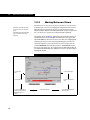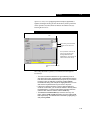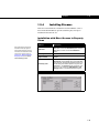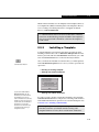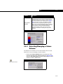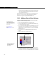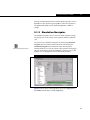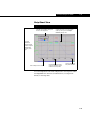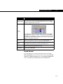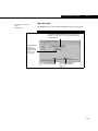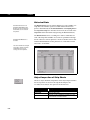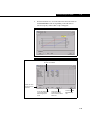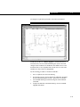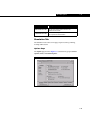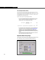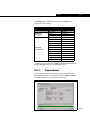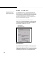
1
2.4 Update Hyprotech is a member of the AEA Technology plc group of companies Copyright Notice The copyright in this manual and its associated computer program are the property of Hyprotech Ltd. All rights reserved. Both this manual and the computer program have been provided pursuant to a License Agreement containing restrictions on use. Hyprotech reserves the right to make changes to this manual or its associated computer program without obligation to notify any person or organization. Companies, names and data used in examples herein are fictitious unless otherwise stated. No part of this manual may be reproduced, transmitted, transcribed, stored in a retrieval system, or translated into any other language, in any form or by any means, electronic, mechanical, magnetic, optical, chemical manual or otherwise, or disclosed to third parties without the prior written consent of Hyprotech Ltd., Suite 800, 707 - 8th Avenue SW, Calgary AB, T2P 1H5, Canada. © 2001 Hyprotech Ltd. All rights reserved. HYSYS, HYSYS.Plant, HYSYS.Process, HYSYS.Refinery, HYSYS.Concept, HYSYS.OTS, HYSYS.RTO, DISTIL, HX-NET, HYPROP III and HYSIM are registered trademarks of Hyprotech Ltd. Microsoft® Windows®, Windows® 95/98, Windows® NT and Windows® 2000 are registered trademarks of the Microsoft Corporation. This product uses WinWrap® Basic, Copyright 1993-1998, Polar Engineering and Consulting. Documentation Credits Authors of the current release, listed in order of historical start on project: Sarah-Jane Brenner, BASc; Conrad, Gierer, BASc; Chris Strashok, BSc; Lisa Hugo, BSc, BA; Muhammad Sachedina, BASc; Allan Chau, BSc; Adeel Jamil, BSc; Nana Nguyen, BSc; Yannick Sternon, BIng; Kevin Hanson, PEng; Chris Lowe, PEng. Since software is always a work in progress, any version, while representing a milestone, is nevertheless but a point in a continuum. Those individuals whose contributions created the foundation upon which this work is built have not been forgotten. The current authors would like to thank the previous contributors. A special thanks is also extended by the authors to everyone who contributed through countless hours of proof-reading and testing. Contacting Hyprotech Hyprotech can be conveniently accessed via the following: Website: Technical Support: Information and Sales: www.hyprotech.com [email protected] [email protected] Detailed information on accessing Hyprotech Technical Support can be found in the Technical Support section in the preface to this manual. Table of Contents Welcome to HYSYS ........................................... vii Hyprotech Software Solutions .............................................vii Use of the Manuals ..............................................................xi Technical Support ..............................................................xix 1 2 3 Interface ........................................................... 1-1 1.1 Interface Basics................................................................. 1-4 1.2 Manoeuvring Through the Interface ................................ 1-20 1.3 Starting a Simulation ....................................................... 1-30 Flowsheet Architecture ................................... 2-1 2.1 HYSYS Environments ....................................................... 2-4 2.2 Sub-Flowsheet Environment ........................................... 2-10 2.3 Templates........................................................................ 2-32 PFD.................................................................... 3-1 3.1 Object Inspection............................................................... 3-4 3.2 PFD Tools ......................................................................... 3-5 3.3 Installing Streams and Operations .................................... 3-9 3.4 Connecting Streams and Operations .............................. 3-10 3.5 Disconnecting Streams and Operations.......................... 3-13 3.6 The Custom PFD Notebook ............................................ 3-15 3.7 Cut/Paste Functions ........................................................ 3-17 3.8 Flowsheet Analysis Using the PFD ................................. 3-19 3.9 PFD Colour Schemes...................................................... 3-30 3.10 Manipulating the PFD...................................................... 3-34 3.11 Adding Annotations ........................................................ 3-52 3.12 Hiding PFD Objects......................................................... 3-54 3.13 Multi Pane PFDs ............................................................. 3-55 3.14 Printing the PFD .............................................................. 3-57 4 Workbook.......................................................... 4-1 4.1 Opening the Workbook...................................................... 4-4 iii 5 6 7 4.2 Installing a Stream or Operation........................................ 4-5 4.3 Accessing Streams or Operations..................................... 4-6 4.4 Deleting Streams or Operations .................................... 4-10 4.5 Setup of the Workbook Page .......................................... 4-11 4.6 Exporting/Importing Workbook Tabs ............................... 4-18 4.7 Sorting Information .......................................................... 4-20 Flowsheet Analysis in HYSYS.......................... 5-1 5.1 Property View Flowsheet Analysis .................................... 5-3 5.2 Navigation ........................................................................ 5-8 5.3 DataBook......................................................................... 5-15 5.4 Object Status Window/Trace Window ............................ 5-46 5.5 Attaching Utilities............................................................. 5-48 Output Control .................................................. 6-1 6.1 Printing in HYSYS ............................................................. 6-4 6.2 Reports ........................................................................... 6-10 6.3 Printing the PFD as a DXF File ...................................... 6-16 6.4 Graph Control.................................................................. 6-18 6.5 Format Editor .................................................................. 6-23 Menu Bar Options ............................................. 7-1 7.1 File .................................................................................... 7-4 7.2 Edit .................................................................................... 7-9 7.3 Simulation........................................................................ 7-10 7.4 Flowsheet ....................................................................... 7-17 7.5 Workbook ....................................................................... 7-25 7.6 PFD ................................................................................ 7-26 7.7 Tools ............................................................................... 7-27 7.8 Column ........................................................................... 7-59 7.9 Basis .............................................................................. 7-59 7.10 Window ........................................................................... 7-60 7.11 Help ................................................................................ 7-62 8 iv Utilities ............................................................. 8-1 8.1 Boiling Point Curves ......................................................... 8-4 8.2 CO2 Solids ...................................................................... 8-10 8.3 Cold Properties ............................................................... 8-12 8.4 Critical Property .............................................................. 8-14 8.5 Data Recon ..................................................................... 8-16 8.6 Depressuring .................................................................. 8-17 8.7 Derivative ........................................................................ 8-40 8.8 Envelope ........................................................................ 8-40 8.9 Hydrate Formation .......................................................... 8-45 8.10 Parametric Utility ............................................................. 8-52 8.11 Pinch Utility...................................................................... 8-65 8.12 Pipe Sizing ...................................................................... 8-69 8.13 ................................................................ Property Table8-73 8.14 Tray Sizing ..................................................................... 8-79 8.15 Tray Sizing Manager ....................................................... 8-89 8.16 User Properties ............................................................ 8-109 8.17 Vessel Sizing ................................................................ 8-114 8.18 Adjust Operation with Utility Target Object.................... 8-118 8.19 References .................................................................... 8-120 Index ..................................................................I-1 v vi Welcome to HYSYS vii Welcome to HYSYS We are pleased to present you with the latest version of HYSYS — the product that continually extends the bounds of process engineering software. With HYSYS you can create rigorous steady-state and dynamic models for plant design and trouble shooting. Through the completely interactive HYSYS interface, you have the ability to easily manipulate process variables and unit operation topology, as well as the ability to fully customize your simulation using its OLE extensibility capability. Hyprotech Software Solutions HYSYS has been developed with Hyprotech’s overall vision of the ultimate process simulation solution in mind. The vision has led us to create a product that is: • Integrated • Intuitive and interactive • Open and extensible Integrated Simulation Environment In order to meet the ever-increasing demand of the process industries for rigorous, streamlined software solutions, Hyprotech developed the HYSYS Integrated Simulation Environment. The philosophy underlying our truly integrated simulation environment is conceptualized in the diagram below: Figure 1 vii Hyprotech Software Solutions The central wedge represents the common parameters at the core of the various modelling tools: • model topology • interface • thermodynamics The outer ring represents the modelling application needs over the entire plant lifecycle. The arrows depict each Hyprotech product using the common core, allowing for universal data sharing amongst the tools, while providing a complete simulation solution. As an engineer you undoubtedly have process modelling requirements that are not all handled within a single package. The typical solution is to generate results in one package, then transfer the necessary information into a second package where you can determine the additional information. At best, there is a mechanism for exchanging information through file transfer. At worst, you must enter the information manually, consuming valuable time and risking the introduction of data transfer errors. Often the knowledge you gain in the second application has an impact on the first model, so you must repeat the whole process a number of times in an iterative way. In a truly integrated simulation environment all of the necessary applications work is performed within a common framework, eliminating the tedious trial-and-error process described previously. Such a system has a number of advantages: • Information is shared, rather than transferred, among applications. • All applications use common thermodynamic models. • All applications use common flowsheet topology. • You only need to learn one interface. • You can switch between modelling applications at any time, gaining the most complete understanding of the process. The plant lifecycle might begin with building a conceptual model to determine the basic equipment requirements for your process. Based on the conceptual design, you could build a steady-state model and perform an optimization to determine the most desirable operating conditions. Next, you could carry out some sizing and costing calculations for the required equipment, then do some dynamic modelling to determine appropriate control strategies. Once the design has become a reality, you might perform some online modelling using actual plant data for "what-if" studies, troubleshooting or even online optimization. If a change at any stage in the design process affects the common data, the new information is available immediately to all the other applications — no manual data transfer is ever required. viii Welcome to HYSYS ix While this concept is easy to appreciate, delivering it in a useable manner is difficult. Developing this multi-application, informationsharing software environment is realistically only possible using Object Oriented Design methodologies, implemented with an Object Oriented Programming Language. Throughout the design and development process, we have adhered to these requirements in order to deliver a truly integrated simulation environment as the HYSYS family of products: For information on any of these products, contact your local Hyprotech representative. HYSYS Product Description HYSYS.Process Process Design - HYSYS.Process provides the accuracy, speed and efficiency required for process design activities. The level of detail and the integrated utilities available in HYSYS.Process allows for skillful evaluation of design alternatives. HYSYS.Plant Plant Design - HYSYS.Plant provides an integrated steady-state and dynamic simulation capability, offers rigorous and high-fidelity results with a very fine level of equipment geometry and performance detail. HYSYS.Plant+ provides additional detailed equipment configurations, such as actuator dynamics. HYSYS.Refinery Refinery Modeling - HYSYS.Refinery provides truly scalable refinery-wide modeling. Detailed models of reaction processes can be combined with detailed representations of separation and heat integration systems. Each hydrocarbon stream is capable of predicting a full range of refinery properties based on a Refinery Assay matrix. HYSYS.OTS Operations Training System - HYSYS.OTS provides real-time simulated training exercises that train operations personnel and help further develop their skills performing critical process operations. Increased process understanding and procedural familiarity for operations personnel can lead to an increase in plant safety and improvements in process performance. HYSYS.RTO Real-Time Optimization - HYSYS.RTO is a realtime optimization package that enables the optimization of plant efficiency and the management of production rate changes and upsets in order to handle process constraints and maximize operating profits. HYSYS.Concept Conceptual Design Application - HYSYS.Concept includes DISTIL which integrates the distillation synthesis and residue curve map technology of Mayflower with data regression and thermodynamic database access. HYSYS.Concept also includes HX-Net, which provides the ability to use pinch technology in the design of heat exchanger networks. Conceptual design helps enhance process understanding and can assist in the development of new and economical process schemes. ix Hyprotech Software Solutions Intuitive and Interactive Process Modelling We believe that the role of process simulation is to improve your process understanding so that you can make the best process decisions. Our solution has been, and continues to be, interactive simulation. This solution has not only proven to make the most efficient use of your simulation time, but by building the model interactively – with immediate access to results – you gain the most complete understanding of your simulation. HYSYS uses the power of Object Oriented Design, together with an Event-Driven Graphical Environment, to deliver a completely interactive simulation environment where: • calculations begin automatically whenever you supply new information, and • access to the information you need is in no way restricted. At any time, even as calculations are proceeding, you can access information from any location in HYSYS. As new information becomes available, each location is always instantly updated with the most current information, whether specified by you or calculated by HYSYS. Open and Extensible HYSYS Architecture HYSYS is the only commercially available simulation platform designed for complete User Customization. The Integrated Simulation Environment and our fully Object Oriented software design has paved the way for HYSYS to be fully OLE compliant, allowing for complete user customization. Through a completely transparent interface, OLE Extensibility lets you: • develop custom steady-state and dynamic unit operations • specify proprietary reaction kinetic expressions • create specialized property packages. With seamless integration, new modules appear and perform like standard operations, reaction expressions or property packages within HYSYS. The Automation features within HYSYS expose many of the internal Objects to other OLE compliant software like Microsoft Excel, Microsoft Visual Basic and Visio Corporation’s Visio. This functionality enables you to use HYSYS applications as calculation engines for your own custom applications. By using industry standard OLE Automation and Extension the custom simulation functionality is portable across Hyprotech software updates. The open architecture allows you to extend your simulation functionality in response to your changing needs. x Welcome to HYSYS xi Use of the Manuals HYSYS Electronic Documentation The HYSYS Documentation Suite includes all available documentation for the HYSYS family of products. All HYSYS documentation is available in electronic format as part of the HYSYS Documentation Suite. The HYSYS Documentation CD ROM is included with your package and may be found in the Get Started box. The content of each manual is described in the following table: Manual Description Get Started Contains the information needed to install HYSYS, plus a Quick Start example to get you up and running, ensure that HYSYS was installed correctly and is operating properly. User’s Guide Provides in depth information on the HYSYS interface and architecture. HYSYS Utilities are also covered in this manual. Simulation Basis Contains all information relating to the available HYSYS fluid packages and components. This includes information on the Oil Manager, Hypotheticals, Reactions as well as a thermodynamics reference section. Steady State Modeling Steady state operation of HYSYS unit operations is covered in depth in this manual. Dynamic Modeling This manual contains information on building and running HYSYS simulations in Dynamic mode. Dynamic theory, tools, dynamic functioning of the unit operations as well as controls theory are covered. This manual is only included with the HYSYS.Plant document set. Customization Guide Details the many customization tools available in HYSYS. Information on enhancing the functionality of HYSYS by either using third-party tools to programmatically run HYSYS (Automation), or by the addition of user-defined Extensions is covered. Other topics include the current internally extensible tools available in HYSYS: the User Unit Operation and User Variables as well as comprehensive instruction on using the HYSYS View Editor. Tutorials Provides step-by-step instructions for building some industry-specific simulation examples. Applications Contains a more advanced set of example problems. Note that before you use this manual, you should have a good working knowledge of HYSYS. The Applications examples do not provide many of the basic instructions at the level of detail given in the Tutorials manual. Quick Reference Provides quick access to basic information regarding all common HYSYS features and commands. xi Use of the Manuals Contact Hyprotech for information on HYSYS training courses. If you are new to HYSYS, you may want to begin by completing one or more of the HYSYS tutorials, which give the step-by-step instructions needed to build a simulation case. If you have some HYSYS experience, but would still like to work through some more advanced sample problems, refer to the HYSYS Applications. Since HYSYS is totally interactive, it provides virtually unlimited flexibility in solving any simulation problem. Keep in mind that the approach used in solving each example problem presented in the HYSYS documentation may only be one of the many possible methods. You should feel free to explore other alternatives. Viewing the Online Documentation HYSYS electronic documentation is viewed using Adobe Acrobat Reader®, which is included on the Documentation CD-ROM. Install Acrobat Reader 4.0 on your computer following the instructions on the CD-ROM insert card. Once installed, you can view the electronic documentation either directly from the CD-ROM, or you can copy the Doc folder (containing all the electronic documentation files) and the file named menu.pdf to your hard drive before viewing the files. Manoeuvre through the online documentation using the bookmarks on the left of the screen, the navigation buttons in the button bar or using the scroll bars on the side of the view. Blue text indicates an active link to the referenced section or view. Click on that text and Acrobat Reader will jump to that particular section. Selecting the Search Index xii Ensure that your version of Acrobat Reader has the Search plug-in present. This plug-in allows you to add a search index to the search list. One of the advantages in using the HYSYS Documentation CD is the ability to do power searching using the Acrobat search tools. The Acrobat Search command allows you to perform full text searches of PDF documents that have been indexed using Acrobat Catolog®. For more information on the search tools available in Acrobat Reader, consult the help files provided with the program. To attach the index file to Acrobat Reader 4.0, use the following procedure: 1. Open the Index Selection view by selecting Edit-Search-Select Indexes from the menu. 2. Click the Add button. This will open the Add Index view. 3. Ensure that the Look in field is currently set to your CD-ROM drive label. There should be two directories visible from the root directory: Acrobat and Doc. Welcome to HYSYS xiii Figure 2 4. Open the Doc directory. Inside it you should find the Index.pdx file. Select it and click the Open button. Figure 3 5. The Index Selection view should display the available indexes that can be attached. Select the index name and then click the OK button. You may now begin making use of the Acrobat Search command. Using the Search Command The Acrobat Search command allows you to perform a search on PDF documents. You can search for a simple word or phrase, or you can expand your search by using wild-card characters and operators. To search an index, first select the indexes to search and define a search query. A search query is an expression made up of text and other items to define the information you want to define. Next, select the documents to review from those returned by the search, and then view the occurrences of the search term within the document you selected xiii Use of the Manuals To perform a full-text search do the following: 1. Choose Edit-Search-Query from the menu. 2. Type the text you want to search for in the Find Results Containing Text box. 3. Click Search. The Search dialog box is hidden, and documents that match your search query are listed in the Search Results window in order of relevancy. 4. Double-click a document that seems likely to contain the relevant information, probably the first document in the list. The document opens on the first match for the text you typed. 5. Click the Search Next button or Search Previous button to go to other matches in the document. Or choose another document to view. Other Acrobat Reader features include a zoom-in tool in the button bar, which allows you to magnify the text you are reading. If you wish, you may print pages or chapters of the online documentation using the File-Print command under the menu. Conventions used in the Manuals The following section lists a number of conventions used throughout the documentation. Keywords for Mouse Actions As you work through various procedures in the manuals, you will be given instructions on performing specific functions or commands. Instead of repeating certain phrases for mouse instructions, keywords are used to imply a longer instructional phrase: These are the normal (default) settings for the mouse, but you can change the positions of the left- and right-buttons. xiv Keywords Action Point Move the mouse pointer to position it over an item. For example, point to an item to see its Tool Tip. Click Position the mouse pointer over the item, and rapidly press and release the left mouse button. For example, click Close button to close the current window. Right-Click As for click, but use the right mouse button. For example, right-click an object to display the Object Inspection menu. Welcome to HYSYS Keywords Action Double-Click Position the mouse pointer over the item, then rapidly press and release the left mouse button twice. For example, double-click the HYSYS icon to launch the program. Drag Position the mouse pointer over the item, press and hold the left mouse button, move the mouse while the mouse button is down, and then release the mouse button. For example, you drag items in the current window, to move them. Tool Tip Whenever you pass the mouse pointer over certain objects, such as tool bar icons and flowsheet objects, a Tool Tip will be displayed. It will contain a brief description of the action that will occur if you click on that button or details relating to the object. xv A number of text formatting conventions are also used throughout the manuals: Note that blank spaces are acceptable in the names of streams and unit operations. Format Example When you are asked to access a HYSYS menu command, the command is identified by bold lettering. ‘Select File-Save from the menu to save your case.’ When you are asked to select a HYSYS button, the button is identified by bold, italicized lettering. ‘Click the Close button to close the current view.’ When you are asked to select a key or key combination to perform a certain function, keyboard commands are identified by words in bolded small capitals (small caps). ‘Press the F1 key on the keyboard to open the context sensitive help.’ The name of a HYSYS view (also know as a property view or window) is indicated by bold lettering. ‘Selecting this command opens the Session Preferences view.’ The names of pages and tabs on various views are identified in bold lettering. ‘Click Composition page on the Worksheet tab to see all the stream composition information.’ The name of radio buttons, check boxes and cells are identified by bold lettering. ‘Click the Ignored check box to ignore this operation.’ Material and energy stream names are identified by bold lettering. Column Feed, Condenser Duty Unit operation names are identified by bold lettering. Inlet Separator, Atmospheric Tower When you are asked to provide keyboard input, it will be indicated by bold lettering. ‘Type 100 in the cell to define the stream temperature.’ xv Use of the Manuals Bullets and Numbering Bulleted and numbered lists will be used extensively throughout the manuals. Numbered lists are used to break down a procedure into steps, for example: 1. Select the Name cell. 2. Type a name for the operation. 3. Press ENTER to accept the name. Bulleted lists are used to identify alternative steps within a procedure, or for simply listing like objects. A sample procedure that utilizes bullets is: 1. Move to the Name cell by doing one of the following: • Select the Name cell • Press ALT N 2. Type a name for the operation. • Press ENTER to accept the name. Notice the two alternatives for completing Step 1 are indented to indicate their sequence in the overall procedure. A bulleted list of like objects might describe the various groups on a particular view. For example, the Options page of the Simulation tab on the Session Preferences view has three groups, namely: • General Options • Errors • Column Options Callouts A callout is a label and arrow that describes or identifies an object. An example callout describing a graphic is shown below. Figure 4 HYSYS Icon xvi Welcome to HYSYS xvii Annotations Annotation text appears in the outside page margin. Text appearing in the outside margin of the page supplies you with additional or summary information about the adjacent graphic or paragraph. An example is shown to the left. Shaded Text Boxes A shaded text box provides you with important information regarding HYSYS’ behaviour, or general messages applying to the manual. Examples include: The resultant temperature of the mixed streams may be quite different than those of the feed streams, due to mixing effects. Before proceeding, you should have read the introductory section which precedes the example problems in this manual. The use of many of these conventions will become more apparent as you progress through the manuals. xvii Use of the Manuals xviii xix Technical Support There are several ways in which you can contact Technical Support. If you cannot find the answer to your question in the manuals, we encourage you to visit our Website at www.hyprotech.com, where a variety of information is available to you, including: • • • • • answers to frequently asked questions example cases and product information technical papers news bulletins hyperlink to support email You can also access Support directly via email. A listing of Technical Support Centres including the Support email address is at the end of this chapter. When contacting us via email, please include in your message: • Your full name, company, phone and fax numbers. • The version of HYSYS you are using (shown in the Help, About HYSYS view). • The serial number of your HYSYS security key. • A detailed description of the problem (attach a simulation case if possible). We also have toll free lines that you may use. When you call, please have the same information available. xix xx Technical Support Centres Calgary, Canada AEA Technology - Hyprotech Ltd. [email protected] (email) Suite 800, 707 - 8th Avenue SW (403) 520-6181 (local - technical support) Calgary, Alberta 1-888-757-7836 (toll free - technical support) T2P 1H5 (403) 520-6601 (fax - technical support) 1-800-661-8696 (information & sales) Barcelona, Spain (Rest of Europe) AEA Technology - Hyprotech Ltd. [email protected] (email) Hyprotech Europe S.L. +34 93 215 68 84 (technical support) Pg. de Gràcia 56, 4th floor 900 161 900 (toll free - technical support - Spain only) E-08007 Barcelona, Spain +34 93 215 42 56 (fax - technical support) +34 93 215 68 84 (information & sales) Oxford, UK (UK clients only) AEA Technology Engineering Software [email protected] (email) Hyprotech Ltd. 0800 7317643 (freephone technical support) 404 Harwell, Didcot +44 1235 434351 (fax - technical support) Oxfordshire, OX11 0QJ +44 1235 435555 (information & United Kingdom sales) Kuala Lumpur, Malaysia AEA Technology - Hyprotech Ltd. Hyprotech Ltd., Malaysia Lot E-3-3a, Dataran Palma [email protected] (email) Jalan Selaman ½, Jalan Ampang +60 3 4270 3880 (technical support) 68000 Ampang, Selangor +60 3 4271 3811 (fax - technical support) Malaysia +60 3 4270 3880 (information & sales) Yokohama, Japan AEA Technology - Hyprotech Ltd. AEA Hyprotech KK Plus Taria Bldg. 6F. 3-1-4, Shin-Yokohama xx Kohoku-ku [email protected] (email) Yokohama, Japan 81 45 476 5051 (technical support) 222-0033 81 45 476 5051 (information & sales) xxi Offices Calgary, Canada Yokohama, Japan Tel: (403) 520-6000 Tel: 81 45 476 5051 Fax: (403) 520-6040/60 Fax: 81 45 476 3055 Toll Free: 1-800-661-8696 Newark, DE, USA Houston, TX, USA Tel: (302) 369-0773 Tel: (713) 339-9600 Fax: (302) 369-0877 Fax: (713) 339-9601 Toll Free: 1-800-688-3430 Toll Free: 1-800-475-0011 Oxford, UK Barcelona, Spain Tel: +44 1235 435555 Tel: +34 93 215 68 84 Fax: +44 1235 434294 Fax: +34 93 215 42 56 Oudenaarde, Belgium Düsseldorf, Germany Tel: +32 55 310 299 Tel: +49 211 577933 0 Fax: +32 55 302 030 Fax: +49 211 577933 11 Hovik, Norway Cairo, Egypt Tel: +47 67 10 6464 Tel: +20 2 7020824 Fax: +47 67 10 6465 Fax: +20 2 7020289 Kuala Lumpur, Malaysia Seoul, Korea Tel: +60 3 4270 3880 Tel: 82 2 3453 3144 5 Fax: +60 3 4270 3811 Fax: 82 2 3453 9772 xxi xxii Agents International Innotech, Inc. Katy, USA Tel: (281) 492-2774 Fax: (281) 492-8144 International Innotech, Inc. Beijing, China Tel: 86 10 6499 3956 Fax: 86 10 6499 3957 International Innotech Taipei, Taiwan Tel: 886 2 809 6704 Fax: 886 2 809 3095 KBTECH Ltda. Bogota, Colombia Tel: 57 1 258 44 50 Fax: 57 1 258 44 50 India PVT Ltd. Pune, India Tel: 91 020 5510141 Fax: 91 020 5510069 Logichem Process Johannesburg, South Africa Tel: 27 11 465 3800 Fax: 27 11 465 4548 Plant Solutions Pty. Ltd. Peregian, Australia Tel: 61 7 544 81 355 Fax: 61 7 544 81 644 Protech Engineering Bratislava, Slovak Republic Tel: +421 7 4488 8286 Fax: +421 7 4488 8286 PT. Danan Wingus Sakti Jakarta, Indonesia Tel: 62 21 567 4573 75/62 21 567 4508 10 Fax: 62 21 567 4507/62 21 568 3081 Ranchero Services (Thailand) Co. Ltd. Bangkok, Thailand Tel: 66 2 381 1020 Fax: 66 2 381 1209 S.C. Chempetrol Service srl Bucharest, Romania Tel: +401 330 0125 Fax: +401 311 3463 Soteica De Mexico Mexico D.F., Mexico Tel: 52 5 546 5440 Fax: 52 5 535 6610 Soteica Do Brasil Sao Paulo, Brazil Tel: 55 11 533 2381 Fax: 55 11 556 10746 Soteica S.R.L. Buenos Aires, Argentina Tel: 54 11 4555 5703 Fax: 54 11 4551 0751 Soteiven C.A. Caracas, Venezuela Tel: 58 2 264 1873 Fax: 58 2 265 9509 ZAO Techneftechim Moscow, Russia Tel: +7 095 202 4370 Fax: +7 095 202 4370 Internet Website: www.hyprotech.com Email: [email protected] xxii xxiii HYSYS Hot Keys File Create New Case Open Case Save Current Case Save As... Close Current Case Exit HYSYS CTRL+N CTRL+O CTRL+S CTRL+SHIFT+S CTRL+Z ALT+F4 Simulation Go to Basis Manager Leave Current Environment (Return to Previous) Main Properties Access Optimizer Toggle Steady-State/Dynamic Modes Toggle Hold/Go Calculations Access Integrator Start/Stop Integrator Stop Calculations CTRL+B CTRL+L CTRL+M F5 F7 F8 CTRL+I F9 CTRL+BREAK Flowsheet Add Material Stream Add Operation Access Object Navigator Show/Hide Object Palette Composition View (from Workbook) F11 F12 F3 F4 CTRL+K Tools Access Workbooks Access PFDs Toggle Move/Attach (PFD) Access Utilities Access Reports Access DataBook Access Controller FacePlates Access Help CTRL+W CTRL+P CTRL CTRL+U CTRL+R CTRL+D CTRL+F F1 Column Go to Column Runner (SubFlowsheet) Stop Column Solver CTRL+T CTRL+BREAK Window Close Active Window Tile Windows Go to Next Window Go to Previous Window Editing/General Access Edit Bar Access Pull-Down Menus Go to Next Page Tab Go to Previous Page Tab Cut Copy Paste CTRL+F4 SHIFT+F4 CTRL+F6 or CTRL+TAB CTRL+SHIFT+F6 or CTRL+SHIFT+TAB F2 F10 or ALT CTRL+SHIFT+N CTRL+SHIFT+P CTRL+X CTRL+C CTRL+V xxiii xxiv xxiv Interface 1-1 1 Interface 1.1 Interface Basics............................................................................................ 4 1.1.1 1.1.2 1.1.3 1.1.4 1.1.5 1.1.6 1.1.7 1.1.8 1.1.9 Windows Functionality ............................................................................. 4 Primary Interface Elements...................................................................... 4 Multi-Flowsheet Architecture/Environments............................................. 5 Objects ..................................................................................................... 6 Structure Terminology ............................................................................ 10 Desktop ...................................................................................................11 Interface Terminology............................................................................. 13 The Property View.................................................................................. 16 Selecting Items ...................................................................................... 19 1.2 Manoeuvring Through the Interface ......................................................... 20 1.2.1 1.2.2 1.2.3 1.2.4 1.2.5 1.2.6 Hot Keys - alt key ................................................................................... 20 Moving Through a View ......................................................................... 21 Moving Between Views .......................................................................... 22 Supplying Input ...................................................................................... 24 Editing Input ........................................................................................... 28 Closing Views......................................................................................... 29 1.3 Starting a Simulation ................................................................................. 30 1.3.1 1.3.2 1.3.3 1.3.4 1.3.5 1.3.6 File Menu ............................................................................................... 30 Basis Manager ....................................................................................... 31 Object Palette ........................................................................................ 33 Installing Streams .................................................................................. 35 Installing Operations .............................................................................. 44 Deleting Streams and Operations .......................................................... 51 1-1 1-2 1-2 Interface 1-3 As you use HYSYS, it will become apparent that you are allowed a high degree of flexibility when performing tasks. In most instances, there is more than one way to accomplish what you are trying to do. Combine this with a consistent and logical approach to how these capabilities are delivered and you are presented with an extremely versatile process simulation tool. The usability of HYSYS can be attributed to four key aspects of its design: 1. First there is the Event Driven operation. This concept combines the power of interactive simulation with instantaneous access to information. Interactive simulation means that information is processed as you supply it, with calculations performed automatically. At the same time, you are not tied to the specific location of the program where you are supplying the information. You can access whatever information you need when you need it. 2. Secondly, Modular Operations are combined with the NonSequential solution algorithm. Not only is information processed as you supply it, but the results of any calculation are automatically propagated throughout the Flowsheet, both forwards and backwards. The modular structure of the operations means that they can calculate in either direction, using information in an outlet stream to calculate inlet conditions. You gain process understanding at every step, since operations calculate automatically. You see the results immediately, thus understanding each piece of the simulation in the greatest possible detail. 3. The third attribute is the Multi-Flowsheet Architecture which allows you to create any number of Flowsheets within a simulation. In addition to satisfying the technical requirement of using multiple property packages within a simulation, this architecture complements the approach to interactive simulation modeling. You can easily break a large simulation into smaller parts to provide a convenient means of focusing your attention on specific sections of the process. 4. Ultimately, what brings all of these features together is the Object Oriented Design of HYSYS. The separation of interface elements (how the information is displayed) from the underlying engineering code means that the same information can be displayed simultaneously in a variety of locations. Each display is tied to the same process variable, so that if the information changes, it is automatically updated in every location. Also, if a variable has been specified, it is shown as a specification in every location - you are not restricted to a single location to change a specification; rather, you can change the specification wherever it is displayed. 1-3 1-4 Interface Basics 1.1 1.1.1 Interface Basics Windows Functionality HYSYS has the same basic features as found in other Windows 95 or NT 4.0 based programs. • Minimize, Maximize/Restore and Close buttons located in the upper right corner of most views. • Close box located in the upper left corner of most views, which contains the normal Windows 3.x menu. Most of the different views found in HYSYS are resizable to some degree. The following list provides a brief description on resizable views: • Minimize, Maximize/Restore and Close buttons available view can be resized vertically and horizontally. • Minimize and Close buttons available - view can be resized vertically only. • Close button or Close and Pin buttons available - view can not be resized. 1.1.2 Primary Interface Elements Although information can be supplied and accessed a variety of ways, there are four primary interface elements for interacting with HYSYS. • The PFD is a graphical environment for building your Flowsheet and examining process connectivity. Process information can be displayed for each individual stream or operation as needed. • The Workbook is a collection of tabs, displaying information in a tabular format. Each Workbook tab displays information about a specific object type, i.e., all streams, pipes, controllers, etc., on a single tab. Multiple tabs for a given object type can be installed, displaying information in varying levels of detail. • The Property View is a single view which contains multiple tabs. HYSYS extensively uses these single views which include all information about a specific object, i.e. an individual stream or operation. • The Summary View displays the currently installed streams and operations. Each of these interface elements, plus the complimentary tools such as the Data Recorder, Strip Charts, Case Study Tool, Plots, etc., are all connected through the model itself. A change made in any location is 1-4 Interface 1-5 automatically reflected everywhere else in HYSYS. In addition, there is basically no restriction on what can be displayed at any time. For example, you can have both the PFD and Workbook open, as well as Property Views for operations and streams. 1.1.3 There are two types of SubFlowsheets: Columns and Templates. Multi-Flowsheet Architecture/Environments As mentioned, HYSYS has been developed around a Multi-Flowsheet Architecture. After you have created the fluid package(s) for your simulation, you enter the Main Flowsheet. In this location, the bulk of the model is created, installing the streams and operations that represent your process. However, you can create a Sub-Flowsheet at any time. Within the Main Flowsheet, the Sub-Flowsheet appears as a single operation with multiple connections. The Main Simulation has no knowledge of what is inside the Sub-Flowsheet. For instance, it could be a refrigeration loop or a decanter system. From the point of view of the Main Flowsheet, the Sub-Flowsheet simply behaves as any other operation; it calculates whenever conditions are changed. The nature of the Sub-Flowsheet gives rise to the concept of Environments. Although a Sub-Flowsheet (template or column) appears as a single operation in the Main Flowsheet, you can, at any time, enter the Sub-Flowsheet to examine conditions in greater detail or make changes. When you do this, you enter the Sub-Flowsheet’s Build Environment. Two things happen at this time. First, the Main Flowsheet is temporarily cached; it will be returned to the exact status when you come back out of the Sub-Flowsheet. Second, the Main Flowsheet solver is temporarily shut down. Calculations will still be performed inside the Sub-Flowsheet, but the results simply won’t be propagated to the rest of the simulation until you come back out. This allows you to focus on a specific aspect of the simulation without having the entire simulation calculate every time conditions change. With this in mind, consider the definition of a Flowsheet (or SubFlowsheet) in the context of the overall program. A Flowsheet is defined by what it possesses: • • • • An independent Fluid Package (optional) A PFD A Workbook Flowsheet Elements (streams and/or operations) 1-5 1-6 Interface Basics This may seem to contradict what has already been stated regarding access to information. However, capabilities have been built into HYSYS to maximize the power of using Sub-Flowsheets without impeding any access to information. No matter where you are in the simulation, you can open any Flowsheet’s PFD or Workbook. Since the Sub-Flowsheets are in essence single operations within the Main Flowsheet, each has its own property view. You can access whatever information resides inside the Sub-Flowsheet through this property view without ever having to enter the Sub-Flowsheet itself. Refer to Section 5.2 Navigation for details on the two navigational tools. All of the Flowsheets within a simulation are tied together through the Navigators. The Object Navigator allows immediate access to the property view for any stream or operation from any location. Similarly, the Variable Navigator allows you to target process variables from any Flowsheet. For instance, you can select variables for inclusion on a Strip Chart or for attachment to logical operations such as Adjusts or Controllers. Figure 1.1 1.1.4 Objects The term Object is used extensively throughout the documentation to refer to an individual stream or operation. Within HYSYS, information associated with an object can be displayed in a variety of ways (Workbook, PFD, Property View, Plot etc.). Through the object oriented design of HYSYS, the information displayed by each interface element is tied to the same underlying object. The result is that if a parameter changes in the Flowsheet it is automatically updated in every location. Object Inspection is a procedure associated with information display. Object displays (for example an icon in a PFD) are tied to appropriate commands for that object, i.e., printing, direct access to a property view, etc. The way in which the pieces and capabilities of the HYSYS interface work together will be illustrated in the following pages. 1-6 Interface 1-7 On the following pages, the major interface elements of HYSYS, with some of the time saving features built into each, are discussed. Each of these elements can be open simultaneously, and offer different representations of the same information. No matter where you are working - supplying information or installing new streams or operations - every interface element automatically updates with the new information. Workbook View Figure 1.2 Double click to open the Property View. Operations attached to a stream can be accessed directly. Object Inspect (right-click area with mouse) the Title Bar to open the Print Datasheet menu, from which you can print the Workbook tab details. Specifications for streams and operations can be supplied directly on the Workbook tab. 1-7 1-8 Interface Basics PFD View Figure 1.3 Double click on any icon to open its Property View. Object Inspect any operation or stream icon to access a menu of options. Object Inspect the PFD by clicking with the secondary mouse button on an empty area of the PFD. You can print the PFD from the Object Inspection menu. Summary View Figure 1.4 Highlight the stream whose Property View you want to open. 1-8 You can also open the Property Views for Unit Operations. Interface 1-9 Object Navigator Figure 1.5 Highlight the Object you wish to view. Press this button to enter the environment of the highlighted Flowsheet. Filter the list for quickly locating a specific object. Press the View button to view the selected object, Off Gas. Stream Property View Figure 1.6 Object Inspect the Title Bar to access the Print Specsheet menu for the Object. Throughout HYSYS, input values appear in blue and calculated values are black. The pages list different views that are available on the current tab. The Status message shows the current status of the Object. The tabs provide a logical grouping of information in the form of pages. These buttons display the property view of the attached unit operation which is Downstream or Upstream of the Stream. 1-9 1-10 Interface Basics 1.1.5 Structure Terminology Before the HYSYS interface usage is explained, some of the terminology that you will encounter will be defined. Every HYSYS case includes certain structural elements. Object Definition Flowsheet Element (or object) A Stream or Operation. Flowsheet A collection of Flowsheet Elements which utilize a common fluid package. In addition, a Flowsheet possesses its own Workbook and PFD. Fluid Package Includes the Property Package, Components (library, pseudo or hypothetical), Reaction Package and User Properties used for Flowsheet calculations. Fluid Packages can be Imported and Exported. Simulation Case A collection of Fluid Package(s), Flowsheets, and Flowsheet Elements which form the model. The Simulation Case can be saved to disk for future reference. The extension used for saved cases is hsc. Session Encompasses every Simulation Case that you have open while HYSYS is running. Special Flowsheet Elements Column Operations and Flowsheet Templates are special Flowsheet Elements in that they are also Flowsheets. A Flowsheet Template can be a Column Sub-Flowsheet or a more complex system. The special capabilities of the Column and Flowsheet Template are: • They have their own Flowsheet, which means they possess their own Fluid Package, PFD and Workbook. • They can be comprised of multiple Flowsheet Elements. • They can be retrieved as a complete entity into any other Simulation Case. 1-10 Interface 1.1.6 1-11 Desktop The figure below shows the basic components of the HYSYS Desktop: Figure 1.7 Menu Bar Button Bar Object Status Window Title Bar Status Bar Trace Window Environment/Mode Label Scroll Bar The main features of the Desktop are: Refer to the next section, Button Bar, for details concerning the various buttons which will be encountered. Object Definition Title Bar Indicates the HYSYS file currently loaded. Menu Bar Provides access to common Flowsheet commands through a pull down menu system. Button Bar Contains various buttons which invoke a specific command when pressed. Environment/Mode Label Indicates the environment and mode in which you are currently working. Status Bar When the mouse pointer is placed over a button in the Button Bar, the Object Palette, or a Property View, a brief description of its function is displayed in the Status Bar. The Status Bar also displays solver status information. Calculation/ Responsiveness Button The Calculation/Responsiveness button allows the user to control how time is spent in updating the screens versus calculations. Scroll Bar Scrolls vertically (in the above case) through the Trace Window. Calculation/Responsiveness Button 1-11 1-12 Interface Basics For more details on the Object Status Window or Trace Window, refer to Section 5.4 Object Status Window/Trace Window. Object Definition Object Status Window/Trace Window The Object Status Window (left pane) shows current status messages for Flowsheet objects while the Trace Window (right pane) displays Solver information. The windows can be resized vertically or horizontally by clicking and dragging the windows frames located between or above them. Button Bar Note that the Button Bar is redrawn depending on the current Environment and Mode. Name The buttons on the Button Bar provide immediate access to the most common commands, which are also available as Menu items. The following is a sample of the buttons found on the various Button Bars. View Description Create a new case. New Case Locate and open an existing case/template/column. Open Case Save the active case. Save Case Open the PFD for the current Flowsheet. PFD Open the Workbook for the current Flowsheet. Workbook Open the Object Navigator. Navigator Simulation Navigator Dynamics Assistant Opens the Simulation Navigator Opens the Dynamic Assistant view. Open the Column Runner view. Column Steady State/ Dynamics Active/Holding Run/Stop Main Environment: Toggles between Active and Holding modes. Green (left) is Active. (Steady State) Column Environment: Toggles between Run and Stop Column Solver. Green (left) is Run. Integrator Integrator toggle. Toggles between Active and Holding. Green (left) is Active. (Dynamics) 1-12 Toggles between Steady State and Dynamic mode. Currently toggled to Steady State mode. Interface Name View 1-13 Description Enter the Basis Environment. Basis Return to the parent Flowsheet from a SubFlowsheet, i.e., the Main Environment from the Column Sub-Flowsheet Environment. Parent Flowsheet Enter the Oil Environment from the Basis Environment. Oil Environment From the Oil Environment, return to the Basis Environment; from the Basis Environment, return to the Main Environment. Leave Environment Some additional things to note about the HYSYS Desktop: • When the mouse pointer is placed over a button, its descriptive name pops up below the pointer and a flyby function is displayed in the status bar. • The Desktop itself has both a vertical and horizontal scroll bar. These are automatically created when necessary. 1.1.7 Interface Terminology Figure 1.8 Accept and Cancel buttons (for Edit Bar input) Drop Down Input Cell Edit Bar Unit Box Pin Scroll Bar Scroll Button Button Input Cell Tabs Object Status Drop Down List 1-13 1-14 Interface Basics The following terminology is used to describe the various HYSYS interface elements: Figure 1.9 Active Highlighted Radio Button Location Minimize, Maximize and Close buttons Group Box Check Box (unchecked) Pages Highlighted Tab 1-14 Object Definition View Any graphical representation found on the Desktop, for example, a Property View for an operation. Button Invokes a command when pressed. Pin Converts a Modal Property View to a Non-Modal Property View. Tabs Provides a logical grouping of information in the form of pages. Pages Provides access to detailed information regarding the selected object. Drop Down List A list of available options for a given input cell. Scroll Bar Provides access to information which cannot be displayed in the current size of a menu or view. Scroll Button Part of the Scroll Bar, allowing you to slide the list up or down, or left or right. Input Cell Location in a View for supplying or viewing information, e.g., stream names, temperatures, etc. In many cases it has a drop down list associated with it. Interface Object Definition Edit Bar Located at the top of a view, and is used for entering or selecting input. The input can be numerical or text. Unit Box Associated with the Edit Bar, this provides a drop down list of units which are applicable for the current input cell. Object Status Each property view shows the status of the associated object with a coloured background (red for a missing parameter, yellow for a warning message and green for OK). Icon A minimized view. Double clicking on one opens the view. Close Box Either closes the view (double clicking), or produces a drop down menu of common Windows commands. Radio Button Always found in groups of at least two; only one can be active at a time. Check Box Items or settings which are On or Off. Selecting the box will turn the function On. Selecting it again turns it Off. Minimize/Maximize Either iconize the current view (minimize), or expand a view to its full size. Active Highlighted Location The current active location is always indicated by highlighting. Group Box Organizational border within a page that groups related functions together. Each group box has its own active location. Matrix A group of cells through which you can manoeuvre with the mouse or the keyboard arrow keys. 1-15 Active View/Active Location Although several views can be displayed on the Desktop at any time, only one view is Active or has Focus. This is indicated by the view’s Title Bar being highlighted. Within that view, there is again only one location that is Active. Depending on the location (cell, button, etc.), how this is displayed can vary. In the previous view, one example of an Active Location is shown. 1-15 1-16 Interface Basics 1.1.8 The Property View Figure 1.10 A Property View is a view that contains multiple tabs, contained within a single border. These are used extensively in HYSYS to allow access to all information associated with an item in a single view. A Property View is Modal by default but can be easily converted to a Non-Modal View by selecting the Pin. A common structure has been adopted for the Property Views. Once you have become familiar with the format and usage of one Property View, each additional one you encounter will behave and be structured in a similar manner. Accessing Property Pages Via the Page Tabs Moving between tabs can be done in several ways: The mouse pointer will not change if the first or last page tab is active AND the pointer is placed to either the left or right, respectively, of the tabs. 1-16 • Select the desired tab with the mouse. • Use the Hot Key combination CTRL SHIFT N, which will cycle you through the tabs (CTRL SHIFT P cycles backwards). • Place the mouse pointer to the direct left or right of the tabs (remaining inside the border of the property view). The cursor will change to a ‘tab switch’ cursor which points in the direction in which the tabs will be cycled. Click the primary mouse button to cycle through the tabs. Interface 1-17 Several time saving features have been built into the Property View: • It will always remember which tab you were last on, returning to that tab automatically the next time you open that view. Each Property View remembers its settings independently; for example, two different streams could automatically open to different tabs. • There are various ways of moving from one tab to the next including selecting the desired tab or by using the Hot Key combination. Supplying or specifying input is accomplished in a variety of manners. Some definitions and terminology will be presented in order to adequately explain the functionality and capabilities of HYSYS. Tabs Each Property View is made up of four or five tabs, which are displayed at the bottom of the View. These tabs provide a logical grouping for the object information. Note that in Figure 1.11, the Design tab is highlighted and appears to be on top of the other tabs, which indicates that this is the current tab. Pages In general, each tab will provide access to more than one page or view The section on the left side of the property view has the same name as the current tab. Within this section is a list of available pages, with the current page being highlighted. The information contained on a specific page may be accessed by simply selecting the page from the list. This ‘page index’ is always present for the specific tab and its appearance is not dependent upon the selection of the page. Cells See Section 1.2.4 - Supplying Input for a more detailed description of the Edit Bar. This is a location in a view for supplying or viewing information, e.g., stream names, temperatures, etc. Cells can be present as single fields (Input Stream cell on a unit operation) or contained within a group as part of a Matrix. An example of Matrix Cells are those found in the Worksheet tab of every unit operation views. In many cases, cells present as a single field have an associated drop down list, indicated by a down arrow next to the field. This produces a list of available options associated with that field. If the cell is in a Matrix, then the drop down list may be in the Edit Bar. 1-17 1-18 Interface Basics Highlight Location The current active location is always indicated by highlighting. Typically this occurs on two levels. First, the actual view (property view for example) will have the Title Bar appear in a different colour than other open inactive views. Second, the active input cell will be indicated with a heavier border, and may also have the contents appear with a highlight. Figure 1.9 shows various types of highlighting. The dashed box in the Toggles group is one type and the enlarged size of the page tab for Simulation is another highlighting indicator. Modal versus Non-Modal Property Views Modal views without pins are called dialog boxes. When a view is Modal you cannot access any other element in the simulation. That is, you cannot select a menu item or view that is not directly part of that Modal view. This functionality is convenient if you do not want to clutter the Desktop with unneccessary views. You will encounter Modal Views without Pins, such as the Input Composition view, which are called dialog boxes. HYSYS uses dialog boxes to retrieve essential information. In essence, you must either input all required information on this view or input nothing in order to proceed. Non-Modal Views do not restrict you in this manner. You can leave a Non-Modal View open and interact with any other view or Menu Item by selecting it. Figure 1.11 Modal View 1-18 Non-Modal View Interface You can set Property Views to be Non-Modal by default in the Session Preferences. 1-19 The Modal View is indicated by the substitution of the Minimize/ Maximize buttons with a Pin. The Non-Modal View has the Minimize/ Maximize buttons in the upper right corner of the window. A Modal View with a Pin can be converted to a Non-Modal View by selecting that Pin. 1.1.9 Selecting Items Selecting refers to either picking a specific item from a list, or invoking a button command. There are four types of selecting in HYSYS. Method Description Selecting a cell Using the mouse, move the cursor to the location and use the primary mouse button to select. Selecting a button Select with the primary mouse button, or move the focus location (using the TAB key or SHIFT TAB combination) and press ENTER. Selecting from a drop down menu or list Move the focus location into the drop down, and use the mouse pointer or keyboard arrows to highlight the selection, then press ENTER to select. Multiple list selections Click and drag the mouse over the items you wish to select (provided they are all sequential in the list). Alternatively, you can highlight sequential items by selecting the first item in the list, holding down the SHIFT key and selecting the last item in the list. If the items are not sequential, select the first item with the primary mouse button and then select additional items with the mouse while holding down the CTRL key. 1-19 1-20 Manoeuvring Through the Interface 1.2 Manoeuvring Through the Interface HYSYS uses Windows conventions regarding interaction between the user and the application. These are described in the following sections. 1.2.1 HYSYS uses a number of Hot Keys for performing commands. For a list, refer to preface of this Manual or to the Quick Reference Guide. The mouse can be used to move the active location to any cell by moving the pointer over the cell and pressing the primary mouse button. Hot Keys - ALT KEY Most Labels, including the items on the Menu Bar, input cell identifiers, and Button labels, have a single letter underlined. This letter works in conjunction with the ALT key as a Hot Key combination, the result of which varies depending on the label type. • For Menu Bar Items (Edit for example), pressing ALT E will open the drop down menu under Edit. • For Input Cell Identifiers (Name, for example), pressing ALT N will move the active location directly to that input cell. • For Buttons (Close, for example), pressing ALT C will invoke the button command. Keep in mind that any keyboard input applies to the active view. For example, if an input cell identifier on the active view has the letter F underlined, you cannot directly open the File Menu by ALT F, as your input will be applied to the active view. The ALT key by itself automatically advances the active location to the first item in the Menu Bar (File). The keyboard arrows move left and right through the row, and the down arrow opens the active menu item. If a drop down menu has underlined letters, you can invoke the command by using that letter only. For example, with the File menu open, you can start a New Case by pressing the N key. Figure 1.12 1-20 Interface 1.2.2 1-21 Moving Through a View When moving through a view using the keyboard functions, you will notice that each input cell and button is accessed sequentially. You can move the active location using the TAB (forward) and SHIFT TAB (reverse) keys. In some instances, such as the Stream property view, HYSYS will automatically advance you to the next input cell after pressing ENTER. If the active location is on a cell in a matrix, the TAB key will not advance you to the next cell in that matrix, but to the next active location in the view. This location may be a button or another group. HYSYS indicates the active location of the cursor in a view in one of three ways. • In the case of a string (Stream Name for example), the entire string will be highlighted. • If the input cell is numerical, a box is placed just inside the cell border. • In the case of a button, the perimeter of the button will be highlighted and the label surrounded by a dashed box. Figure 1.13 Shows a text cell as the Active Location. If Outlet was the active cell, pressing would advance to Energy, while SHIFT TAB would move back to Inlet. TAB If Delete was the active location, pressing TAB would advance the highlight to Inlet, while SHIFT TAB would reverse the highlight to the On/Off checkbox. 1-21 1-22 Manoeuvring Through the Interface 1.2.3 CTRL F6 or CTRL TAB will make the next View in the sequence Active. CTRL SHIFT F6 or CTRL SHIFT TAB reverses the direction of the sequence. Moving Between Views The easiest way to move from one view to another is to use the mouse. To make a view or icon active, simply press the primary mouse button when the cursor is placed over the view or icon. However, because HYSYS maintains all views (including minimized views) in a sequenced list, you can move to another view using keyboard commands. The graphic shown in Figure 1.14 illustrates the method by which you can move between views. If P-100 is the initial active view, press CTRL F6, and the PFD icon becomes the active view. This is now highlighted, indicating the active location. Pressing CTRL F6 again forces the next view in the sequence to become the active location. In this case, the iconized Workbook. Press CTRL F6 once more, and P-100 will become the active view. In this case, the sequenced views (PFD and Workbook) are minimized. Minimized views which become active are denoted by a highlighted title bar. Figure 1.14 1. Initial Active View. 6. Active View again. 2. Press CTRL F6. 5. Press CTRL F6 once more. 3. The PFD becomes the Active View (indicated by highlighting the icon name). 1-22 Press CTRL F6 again. 4. The Workbook becomes the Active View. Interface 1-23 If all three of the preceding views are open, the view will be similar to that shown below. Sequencing through these will overlay the active view on top of the previously active view (instead of highlighting). In the following example, P-100 is the active location (notice it is on the top) and its name, P-100, is also highlighted. Pressing CTRL F6 makes Workbook the active location. When Workbook becomes the active location, P-100 will be hidden behind the PFD view. Figure 1.15 This will become the Active location by pressing CTRL F6 Active View Moving to the Up/Downstream Object Downstream and Upstream Buttons The stream property view presents a special case of moving to a different view is encountered when it is active. From the stream view, the property views for the upstream and downstream objects can be directly accessed by the Upstream Object or Downstream Object button, respectively. 1-23 1-24 Manoeuvring Through the Interface 1.2.4 Supplying Input Text Input When the required input is a Name (a stream or operation), you can either supply the input directly via the keyboard, or in most cases choose from a drop down list of applicable responses. If you are supplying the input from the keyboard, (e.g. creating a new stream), simply enter the text and press ENTER. You can override the filtered list by typing in the desired name directly. The drop down list displays existing objects. By default, HYSYS will filter the list of available streams and operations to include only those applicable to the current situation. For example, when selecting a stream as an operation feed, only unconnected streams or streams that are outlets of other operations will be shown. The following is a description of how to use drop down lists to select existing items. Depending on the type of cell that has focus, the drop down list may appear next to the cell or in the Edit Bar. A drop down list directly tied to a cell is signified by a down arrow next to the cell (i.e. the Outlet cell on the Mixer property view). If a cell’s drop down list is in the Edit Bar, then a down arrow will appear in the Edit Bar when the cell has focus. For instance, when a cell in the Inlets matrix on the MIX-100 property view has focus, the Edit Bar contains a drop down list. Figure 1.16 1-24 Interface 1-25 Numerical Input If the input is numerical, the approach is slightly different. Views that accept numerical input use the Edit Bar, which is redrawn to include a Unit Box. The Unit Box will display the current default unit for the input cell property. When you begin supplying a number for a numerical input cell, your input is echoed in the Edit Bar. When you have supplied the number and have pressed ENTER, HYSYS assumes that the default unit was correct and transfers the value back into the input cell. Figure 1.17 As numerical input for a parameter (e.g., Delta P) is supplied for the first time, it is echoed in the Edit Bar at the top of the view. Delta P cell is presently empty. The numerical value entered in the Edit Bar (10 kPa) will be displayed here. Unit Box shows the default units. While HYSYS is matching your input to the list of units, you can stop entering text and use any of the other methods for locating the unit (such as selecting it with the mouse, using the up and down arrows etc.). If you are supplying the number with a different unit than the default, there are two methods available for identifying it. Method Action Keyboard Input a space after the number and then begin typing in the unit. The unit becomes highlighted in the Unit Box drop down list. Mouse After supplying the numerical value, but before pressing ENTER, open the drop down list and locate the desired unit 1-25 1-26 Manoeuvring Through the Interface Figure 1.18 Display the Unit Box drop down list after supplying a numerical value by selecting the down arrow. The Scroll Bar can be used to locate the required unit. As you supply more of the unit, the highlight will move through the list covering the unit the most closely matches your input. Pressing ENTER accepts both the number and the unit. The value is recalculated using the default unit and is transferred to the Active Location. When you begin entering the units, the Unit Box drop down menu automatically opens. Drop Down Lists and Scroll Bars Drop down lists are used extensively in HYSYS to provide an efficient means of locating existing streams, operations, or units. These menus can be accessed either via the mouse, or by using keyboard input. Once a drop down list is opened, you manoeuvre through the list using the mouse or keyboard. The F2 key opens the drop down list in the Edit Bar. A drop down list for a Text input cell (valve inlet for example), can be opened at any time by using the primary mouse button to select the applicable arrow box. This not only opens the menu, but moves the active location to that input cell. You can also open the drop down list for the current active cell by pressing the keyboard down arrow. If the stream is being attached for the first time, the highlight in the drop down list will be at the top of the list. If the input cell already has a stream in it, the highlight will be on that stream. For a numerical input cell, the drop down list is located next to the Edit Bar at the top of the view, and contains the Unit Box. This automatically 1-26 Interface 1-27 opens as soon as you stop supplying numerical input (signified by a <space>) and begin entering the unit. Alternatively, the drop down list can be opened at any time (which terminates the number entry) by selecting the arrow box. Figure 1.19 Click here to move up one item Click and drag to scroll the Menu Click here to move down one Page The Up and Down arrows can be used to move through the list. Pressing ENTER selects the highlighted item. The mouse can be used to select the item directly. Click here to move down one item Once a drop down list is opened, you can manoeuvre through it in several ways: • The most convenient method is via type-matching. Once a drop down list is open, keyboard input is interpreted to find the first menu item which best matches your input. As you continue to supply input, the matching continues. Pressing ENTER terminates the string and accepts the highlighted item. You can also use the keyboard arrow keys to move to any item. • If the menu contains six items or less, it appears without a scroll bar. In this case, you can use the mouse to directly select the desired item, or use the up and down keyboard arrows to mark the item and then select it with the ENTER key. • The PAGE UP and PAGE DOWN keys move the menu by one page, and the HOME and END keys take you to the first and last item respectively. The desired item is selected by highlighting it and pressing ENTER. 1-27 1-28 Manoeuvring Through the Interface • The Scroll Bar/Scroll Button provides similar functionality. Selecting the Up and Down Scroll Arrows advance the menu by one item. The scroll button can be selected with the primary mouse button and dragged up and down to quickly scroll the menu. • Selecting the space between the scroll button and the scroll arrow advances the menu up or down one page. The desired item can then be selected with the primary mouse button. 1.2.5 Editing Input Editing input can be done in two ways. When the input cell is active, any information you supply will overwrite the previous input. Likewise, you can use the drop down list to replace previous input. Figure 1.20 Cancel Change Accept Change Insertion Point If you want to make changes to previously supplied input, you can make an insertion point. Input Cell location. The value in the Edit Bar is converted to default units, in this case, kPa. 1-28 Interface 1-29 You have a choice when editing numerical input. To make an Insertion Point somewhere in the number, use the mouse or press F2 and use the arrow keys. You can then make selective changes. • If you simply type in a new value and press ENTER, HYSYS accepts the input and assumes it is in the default units. • You can change the units using the methods described previously. • Another method is via selective modification. With this route, you place an insertion point somewhere in the string and make selective changes. Pressing ENTER or selecting the Accept Change box accepts the changes, while you can abort them by selecting the Cancel Change box. 1.2.6 Closing Views There are four ways to close a view. • Double click on the Close Box in the upper left hand corner of the view. • Click once on the Close Box to open the drop down menu. The Close function in this drop down menu has the C underlined. Press the C on the keyboard to close the view. • CTRL F4 closes the active view. • Click on the Close button in the upper right hand corner of the view. Figure 1.21 Close Box Close Button 1-29 1-30 Starting a Simulation 1.3 Starting a Simulation When starting a New simulation, the first thing you need to do is create a New Case. You can do this through the File option in the Menu Bar or using the New Case button. New Case Button 1.3.1 File Menu Before proceeding with the installation of a new case, the options available under File in the Menu Bar will be explained. These options are the general commands associated with any file - saving, printing, etc. For more information about the File Menu, refer to Section 7.1 - File. See Chapter 6 - Output Control for more information on printing. 1-30 Command Definition Starting (New/Open) Creates a New HYSYS case or Opens an existing one. Saving (Save/Save As/Save All) When saving a case for the first time, choose the Save command. Supply the file name and the location (file path) to which you want to save the file. If the case has been previously saved, this command updates the information on disk. If you want to change the file name or location, use the Save As command. The Save All command can be used to save all HYSYS cases currently open. You are asked to select which cases should be saved. Closing (Close Case/ Close All) Close Case closes the current simulation; you are first prompted to save it. Close All accesses a dialog of cases currently in memory, allowing you to specify which should be closed. Again, you will be prompted to save the cases first. Printing (Print/Print Snapshot/Printer Setup) Print accesses a dialog of options for printing Specsheets for the active object. Print Snapshot prints a snapshot of what currently appears in the HYSYS active window. Printer Setup is used to select the default printer, print orientation, paper size, etc. It is similar to the Printer Setup commands in other Windows applications. Interface 1.3.2 1-31 Basis Manager When you start a New Case, HYSYS places you directly into the Simulation Basis Manager. From this location you can manipulate every Fluid Package in the simulation. The minimum steps required to create a Fluid Package for your simulation are described. Figure 1.22 Refer to Chapter 1 - Fluid Package of the Simulation Basis Manual for more information. From the Basis Manager, select the Add button to add the Fluid Package to the new case. Prior to entering the Main Environment, you must fully define at least one fluid package by selecting a property package and a set of components. HYSYS places you on the Prop Pkg page of the Fluid Package. 1-31 1-32 Starting a Simulation From the Base Property Package Selection group, select a Property Package to use with this case. Figure 1.23 The next thing to do is select the components you are going to use in the case. Select the Components tab. Figure 1.24 1-32 Interface 1-33 Once the Components and the Property Package have been selected, press the Close button to return to the Basis Manager. From here, press the Enter Simulation Environment button to move to the Main Environment. Now that you have entered the Main Environment, you need to install streams and operations in the case. 1.3.3 Object Palette The Object Palette can be used to install streams and operations. You can open or close the Palette from the Flowsheet option in the Menu Bar, or by using the F4 Hot Key. In the Main Flowsheet or Template Sub-Flowsheet, every operation available in HYSYS is accessible via the Palette, (except those specifically associated with Columns such as tray sections, reboilers, etc.). A separate Palette is produced when you are inside the Column Sub-Flowsheet. From top to bottom, the Palette is organized into the following categories: • • • • • • • • • • • Object Palette Streams Vessels (2 and 3-phase separators, tank) Heat Transfer Equipment Rotating Equipment (compressor, expander, pump) Piping Equipment Solids Handling Reactors Prebuilt Columns Shortcut Columns Sub-Flowsheets Logicals Buttons on the object palette that display an arrow pointing to the side represent general buttons. For instance, the Solid Ops and General Reactors buttons each will bring up a secondary palette displaying buttons for more specific unit operations. As shown, you can select a Gibbs Reactor, an Equilibrium Reactor or a Conversion Reactor after pressing the General Reactors button. General Reactors 1-33 1-34 Starting a Simulation Each operation has a representative icon. In addition, when you place the mouse pointer over top of any button, the flyby description of what operation the icon represents is displayed both below the pointer and at the bottom of the HYSYS Window in the Status Bar. Installing Streams and Operations via the Palette Add Button You can install a single stream or operation from the Palette by double clicking on the icon for the object you want to install. You can also use the Add button at the top of the Palette. First, click on the button for the Object you wish to install, then click on the Add button. This displays the Property View for the Object type chosen. You can install multiple Streams and Unit Operations from the Palette by using the Lock button. The procedure for this is as follows: Lock Button Cancel Button 1. Click on the Lock button at the top of the Palette. 2. With the primary mouse button, click on the Icon for the Stream or Operation you want to install. 3. Select the Add button to install the stream or operation. 4. You can repeat this as many times as necessary. To deactivate the chosen Object button when in locked mode, press the Cancel button or select a different Object. The Object button returns to its normal state (changes from light grey to dark grey). To remove the Lock function, click on the Lock button again. 1-34 Interface 1.3.4 1-35 Installing Streams There are several methods to install new streams in HYSYS. Some of these methods immediately open the Stream Property View upon installation and others do not. Installation with Direct Access to Property Views Note that both the menu bar and the F11 hot key options will install a material stream. To convert the material stream to an energy stream, refer to Section 2.1 - Material Stream Property View of the Steady State Modeling Guide. Method Description Menu Bar New streams can be installed into the case via the Menu Bar. Choose the Flowsheet option from the Menu Bar, and then choose the Add Stream option. Hot Keys Press F11. Object Palette Double click on the stream icon in the Object Palette. Summary View Open the Select Summary view by selecting Summaries from the Tools option in the Menu Bar. From this view, highlight the Flowsheet to which you will be adding the stream operation and press the View button. The Summary view will appear, from which you can choose the Add Material or Add Energy buttons in the Flowsheet Streams group. Figure 1.25 1-35 1-36 Starting a Simulation Installation Without Direct Access to Property Views Method Description Workbook Position the cursor in the **New** cell of a Streams Type Workbook tab. Type in the new stream name. You can now proceed to enter values for the default stream variables. Operation Property View You can supply a new stream name in an Input Cell for an operation, which automatically creates the stream. Both Material and Energy Streams can be added to the case via the Object Palette. Material Stream Button (Blue) • With the primary mouse button, click on the Stream Icon in the palette (Material or Energy). Move the cursor to the area on the PFD where the Stream is to be placed. Press the primary mouse button to complete the installation. Object Palette to PFD Energy Stream Button (Red) or • From the Object Palette, click (with the secondary mouse button) and drag the stream icon to the desired location in the PFD. Release the secondary mouse button to drop the stream on the PFD. To access the Property View for a stream, do one of the following: Refer to Section 3.8 Flowsheet Analysis Using the PFD for more information on accessing Property Views from the PFD. Refer to Section 5.2.1 - Object Navigator for information on accessing the navigator and its functions. 1-36 • Double click on a Stream cell (any cell except a flow cell, which accesses the Input Composition dialog) in the Workbook. • Double click on the Icon in the PFD. • Object inspect (with the secondary mouse button) a stream cell in the Workbook. Choose View from the menu that appears. • Object inspect the Icon in the PFD and choose View Properties. • Open the Object Status Window (left pane). Double click on the message related to the stream. • Access the Summary view, highlight the stream name in the Flowsheet Streams group and press the View button. Interface 1-37 • Access the Object Navigator. Select the Streams radio button and highlight the name of a stream in the Streams group. Press the View button. Figure 1.26 Spec Stream As On each Stream Property View, there is a Define from other Stream button. This allows you to copy the existing specifications from another stream into the present stream. When you press this button, the Spec Stream As view appears. Figure 1.27 In the Copy Stream Conditions group, you can select a maximum of two variables in the first group: vapour fraction, temperature, pressure, 1-37 1-38 Starting a Simulation molar enthalpy, or molar entropy. These will become the user defined variables for the stream. If you wish to have the composition and/or flow copied, select the appropriate box. From the Flow Basis group, you can select which flow type will be the user defined flow. Installing a Stream - Example Material and Energy streams can be installed with any one of the methods mentioned previously. For this example, the default units are SI, the property package is NRTL and the components are Water and Methanol. The following procedure will outline the installation of a Stream: 1. Double click on the Material Stream button in the Object Palette. This brings up the Stream property view, which will have been auto-named as 1. Figure 1.28 1-38 Interface 2. 1-39 The Stream Name cell will have focus. You can type in a new name, for example, Stream1. Your input will be echoed in the Edit Bar. Pressing ENTER transfers your input back to the Stream Name cell. Figure 1.29 3. Nothing will be supplied for Vapour/Phase Fraction. Press the keyboard down arrow to move the highlight to the Temperature cell. 1-39 1-40 Starting a Simulation 4. With the highlight on the Temperature cell, type in 60. This appears in the Edit Bar. In the Unit List, C appears because this is the default SI temperature unit. Press ENTER to accept the entry. Figure 1.30 5. 1-40 The highlight will now be on the Pressure cell. You want the pressure for this stream to be 0.5 bar. The default SI unit for pressure is kPa, so you must change the pressure unit to bar. Type in 0.5 followed by a Space, and the letter b. The Unit Box drop down list will appear and bar will be highlighted. Press ENTER to accept the units. Interface 1-41 Figure 1.31 6. Notice that the value transferred into the Pressure cell is 50 kPa, as kPa is the default display unit for pressure. 7. You will now be on the Molar Flow cell. Type in a value of 100 kgmole/hr and press ENTER. Notice that the stream still hasn’t flashed, because we have not supplied a composition. Figure 1.32 1-41 1-42 Starting a Simulation 8. With the primary mouse button, select the Composition page. To supply or edit the composition, either select a cell and enter a value or press the Edit button. The Input Composition view will be displayed. Figure 1.33 Note that you could also double click on the appropriate flow cell (mole, mass, or liquid volume) on the Conditions page and access the following Input Composition view directly. 1-42 Interface 9. 1-43 Select the Mole Fractions radio button prior to the input of values. Enter a Mole Fraction of 1.0 for Water and 1.0 for Methanol. Figure 1.34 10. Press the Normalize button. Notice that the Total becomes 1.0, as each component is assigned a mole fraction of 0.5. 11. Press the OK button to return to the stream property view. The mole fractions entered are now present on the Composition page. 12. Select the Conditions page. The stream will have flashed. Notice the status message shows OK. Figure 1.35 1-43 1-44 Starting a Simulation 13. Note that it is a two phase stream. Use the horizontal scroll bar to move to the Aqueous and Vapour Phase information of the stream. You can also resize the view horizontally to display all three phases, mixed, aqueous, and vapour. Remember that if the stream property view is Modal, you must press the Pin button to make the view Non-Modal before you can resize it. To resize the view, place the mouse pointer on the border and drag horizontally. The resized view is shown next. Figure 1.36 More information regarding the stream properties can be found on the other pages of the view. 1.3.5 Installing Operations As with Streams, there are various ways to install Unit Operations in HYSYS. Some of these methods immediately open the operation’s Property View and some do not. 1-44 Interface 1-45 Direct Property View Access Method Description Menu Bar New Unit Operations can be installed into the Case via the Menu Bar. Choose the Flowsheet option from the Menu Bar, and then select Add Operation. Hot Key Press F12. Summary View Open the Select Summary view by selecting Summaries from the Tools option in the Menu Bar. From this view, highlight the Flowsheet in which you will be adding the operation and press the View button. The Summary view will appear, from which you can choose the Add button in the Unit Operations group. You can directly access the Summary view by pressing the Summary View button in the Button Bar Workbook, Unit Ops Page From the Unit Ops page of the Workbook, press the Add UnitOp button. All of these methods will display the UnitOps view, listing all the available Unit Operations. Upon selecting the Unit Operation, HYSYS will produce the applicable Property View. Figure 1.37 Use the radio buttons to select the category of Unit Operation you want to add. When the desired Unit Operation is highlighted, press the Add button. Unit Operations available according to the radio button chosen. 1-45 1-46 Starting a Simulation Using the Object Palette to install an operation can also give you direct Property View access. Method Description Two methods are available: Object Palette • Double click on the operation icon in the Object Palette. Click on the desired operation and press the Add button at the top of the Palette. Without Direct Property View Access Refer to Section 4.5.2 - Editing a Workbook Tab for information concerning the custom Workbook tab. Object Description Workbook Create a specific tab for the operation type you want to add in the Workbook. For example, add a Valves tab to the Workbook for all the valves in the Flowsheet. Once you have the Operation tab in the Workbook, you will notice that the default variables for the Operation are shown. In the cell displaying **New**, enter the name for the new operation. Two methods are available: For a custom Unit Operation Workbook tab, only one type of Unit Operation is allowed. Object Palette to PFD • With the primary mouse button, click on the Icon in the Palette for the operation you want to install. Move the cursor to the PFD area where you want to place the operation, and press the primary mouse button to complete the installation. • With the secondary mouse button, click on the Icon in the Palette for the operation you want to install. Hold the mouse button down and drag the cursor into the PFD. Position the cursor where you want to place the operation and release the button. To access the Property View for an operation, do one of the following: • On a custom Unit Operation Workbook tab (i.e. Valves page), double click on one of the Unit Operation’s cells. • Double click on the Icon in the PFD. • Object inspect (with the secondary mouse button) a cell on a custom Unit Operation Workbook tab. Choose View from the menu that appears. • Object inspect the Icon in the PFD and choose View Properties. • On the Unit Ops tab of the Workbook, highlight the operation and press the View UnitOp button. • On the Unit Ops tab of the Workbook, double click on the Name, Object Type or Calc. Level cell for the operation. • Open the Object Status Window (left pane). Double click on the message related to the unit operation. • Open the Summary view, highlight the operation and press the View button in the Unit Operations group. 1-46 Interface 1-47 Installing a Unit Operation - Example Unit Operations can be installed using any of the methods just described. This example demonstrates the installation of a TEE. It is assumed that two streams have already been installed, Stream1 and Stream2. The default units are SI. 1. Double click on the TEE button in the Object Palette. This opens the Property View, for the TEE which has been automatically named TEE-100. Focus is currently on the Inlet cell. Figure 1.38 TEE Button 2. You can either type in the Feed Stream name, which can be an existing stream or a new stream, or choose a stream from the drop down list. In this case, use the drop down list to choose one of the streams already installed. With the mouse, click on the down arrow next to the cell to open the drop down list. Figure 1.39 1-47 1-48 Starting a Simulation 3. From the drop down list, select Stream1. This is now installed as the Feed stream to the TEE. The stream name in the Feed cell is highlighted and the cursor has not moved from this location. The status message has changed from Requires a feed stream to Requires a product stream. 4. Move the cursor to the first cell in the Outlets group. You can have as many product streams as you want. Again, you can supply streams by typing a name into the cell, or by selecting already installed streams from the drop down list in the Edit Bar. Each method will be used to install one product stream. Figure 1.40 1-48 Interface You can also select items from the drop down list by simply clicking on them with the primary mouse button. 5. 1-49 Click on the down arrow to the right of the Edit Bar to open the drop down list. The only stream appearing in the drop down list is Stream2. Highlight it using the arrow keys and press ENTER to accept it as an input. When you do this, HYSYS places this stream as the first stream in the Outlets group. Figure 1.41 6. In the Outlets group, move the highlight to the next cell, which is ready for a new input. Now type in the name Stream3. Because it is a new stream, HYSYS automatically installs it in the simulation. The TEE connections are now complete. The status message displays Unknown Splits. Figure 1.42 1-49 1-50 Starting a Simulation 7. Go to the Parameters page to supply the split fraction for each product stream. The two Product streams, Stream2 and Stream3 appear on this page. The sum of the Flow Ratios must equal 1.0, so you only need to supply one ratio. HYSYS will calculate the other ratio by difference. Move the cursor to the Stream2 Flow Ratio cell and type in 0.40. Figure 1.43 1-50 8. HYSYS has calculated the Flow Ratio of Stream3 to be 0.60. In HYSYS, calculated values appear in black and supplied values appear in blue. In this view, 0.40 is shown in blue, and 0.60 in black. Since the TEE is being used in Steady State, this is all the information needed. The status message shows OK. 9. Press the Close button to exit the Property View. Interface 1.3.6 Remember, once a stream or operation is deleted, it cannot be recovered. 1-51 Deleting Streams and Operations Property View You can delete any stream or operation through its Property View by selecting the Delete button. Workbook From the Workbook, you can delete Streams or Operations in various ways, depending on the type of Workbook tab which is being viewed: • On any Workbook tab, double clicking on the operation or stream accesses the Property View for the object. By pressing the Delete button on the property view, the object will be deleted. • On any Workbook tab but the Unit Ops page, select the item with the secondary mouse button which provides the Object Inspection menu. Selecting Delete from this menu deletes the object. • Highlight the object Name cell and press DELETE on the keyboard. • On the Unit Ops tab only, highlight the operation and press the Delete UnitOp button. PFD To delete streams and operations from a PFD, you can: • Double click on the operation or stream accesses the Property View for the object, from which you can delete it by pressing the Delete button. • Select the item with the secondary mouse button which provides the Object Inspection menu. Selecting Delete from this menu deletes the object. • Select the object and press DELETE on the keyboard. 1-51 1-52 Starting a Simulation Summary View There are separate Delete buttons for the stream and operation groups. Once inside the Summary View, you can delete either streams or operations. The Flowsheet Streams group lists all the streams present in your case. Similarly, the Unit Operations group lists all the operations in your case. Highlight the object you want to delete and then press the Delete button. You can highlight multiple streams or operations, and then delete them at the same time. Figure 1.44 No matter which of the above methods you use for deleting objects, HYSYS will prompt you for confirmation before deleting the object. This confirmation requires you to select either Yes or No from the message box that appears. 1-52 Flowsheet Architecture 2-1 2 Flowsheet Architecture 2.1 HYSYS Environments .................................................................................. 4 2.1.1 2.1.2 2.1.3 2.1.4 Basis Environments ................................................................................. 4 Main Simulation Environments................................................................. 5 Related Environments.............................................................................. 7 Advantages of Using Environments ......................................................... 9 2.2 Sub-Flowsheet Environment..................................................................... 10 2.2.1 2.2.2 2.2.3 2.2.4 2.2.5 2.2.6 2.2.7 Sub-Flowsheet Entities ...........................................................................11 Sub-Flowsheet Advantages ....................................................................11 Multi-Level Flowsheet Architecture ........................................................ 12 Flowsheet Information Transfer ............................................................. 14 Sub-Flowsheet Property View................................................................ 15 Installing a Sub-Flowsheet ..................................................................... 22 Decanter Sub-Flowsheet Example......................................................... 23 2.3 Templates.................................................................................................... 32 2.3.1 2.3.2 2.3.3 2.3.4 Template Information ............................................................................. 32 Creating a Template Style Flowsheet..................................................... 36 Installing a Template .............................................................................. 37 Example - Refrigeration Loop Template................................................. 39 2-1 2-2 2-2 Flowsheet Architecture 2-3 HYSYS has been engineered with a multi-level flowsheet architecture tightly integrated within a framework of simulation environments. A direct result of this powerful design is that although HYSYS allows you to interact with an installed sub-flowsheet operation as if it were a simple black box, you can easily delve deeper using the sub-flowsheet’s simulation environment when more interaction is required. This intuitive simulation environment framework allows you to focus on the task at hand by providing completely separate Desktops for each environment. It also provides a natural mechanism for HYSYS to be exploited in providing peak computational efficiency for the user. The net result is that potentially complex flowsheets installed as subFlowsheet operations behave in a familiar and consistent manner, just like the other "normal" unit operations in HYSYS. HYSYS also supports a natural extension to the sub-flowsheet concept the idea of a Process Template. Basically, a Template is a complete Flowsheet that has been stored to disk with some additional information included that pertains to hooking that flowsheet up as a sub-flowsheet operation. Typically a Template is representative of a plant process module or a portion of a process module. The stored Template can subsequently be read from disk and efficiently installed as a complete sub-flowsheet operation any number of times into any number of different simulation cases. The versatility of the HYSYS sub-flowsheet is extended by the capability of assigning it a separate Fluid Package. For example, this option will enable you to more rigorously model plant utilities such as cooling water and steam circuits as separate flowsheets with dedicated Steam Table property packages. Column Sub-Flowsheets - A Special Case There is another feature that the multi-level flowsheet architecture makes possible in HYSYS. This is the extension of HYSIM’s traditional or modal style of Column operation into the vastly more flexible and powerful Column Sub-Flowsheet Operation incorporated in HYSYS. Column sub-flowsheets are a distinct class of sub-flowsheet due to their ability to provide a simultaneous Flowsheet solution. Even though they are different, they are created and accessed much like normal subflowsheets, and Column Templates can also be created and later imported into other simulations. However, the Column sub-flowsheet’s property view and the Column’s simulation environment are very different, as they are suited specifically for designing Columns rather than general processes. 2-3 2-4 HYSYS Environments Although a lot of the general sub-flowsheet information presented in this chapter also applies to the Column sub-flowsheet, the Column Sub-Flowsheet Operation is discussed specifically and in-depth in Chapter 7 - Column of the Steady State Modeling manual. 2.1 The environments help you maintain peak efficiency while you are working with your simulation, by avoiding the execution of redundant calculations. HYSYS Environments The environment design concept is one of the cornerstones on which HYSYS is built. These environments allow you to access and input information in a certain area ("environment") of the simulation, while other areas of the simulation are put on hold. The other areas won’t proceed with steady state calculations until you are finished working in the area of interest. Since the HYSYS integrator is time-step based, the environments have no impact on dynamic calculations. Separate Desktops are available with each environment. Each of these Desktops includes an appropriate Menu Bar, Button Bar and Home View(s) specifically designed for interaction with their particular environment. The Desktops also remember the views that were open on them, even when their associated environment is not currently active. When moving from one environment to another, they provide a mechanism for quickly and automatically "putting away" what ever views you have open in one environment, and "bringing up" the views that were open in the other environment. This feature is particularly useful when working with large Flowsheets. The environments in HYSYS can be loosely grouped into two categories for the purposes of discussion: Basis environments and Main simulation environments. 2.1.1 Basis Environments Within this category, there are the following two types of environments: • • Simulation Basis Environment Oil Characterization Environment The Simulation Basis Environment Whenever you begin a HYSYS simulation, you automatically start in the Simulation Basis environment. Here you can create, define and modify Fluid Packages to be used by the simulation’s Flowsheets. In general, a Fluid Package contains at minimum a Property Package, as well as 2-4 Flowsheet Architecture 2-5 library and/or hypothetical components. Fluid Packages may also contain information such as reactions and interaction parameters. The Desktop for the Simulation Basis environment is specifically suited to the task at hand as reflected by the available choices of buttons on the Button Bar (Figure 2.1) and the designation of the Simulation Basis Manager view as the Home View. Figure 2.1 The Oil Characterization Environment The Oil Characterization environment allows you to characterize petroleum fluids by creating and defining Assays and Blends. The Oil Characterization procedure generates petroleum pseudo components for use in your Fluid Package(s). The Oil environment is unique in that it is accessible only from the Simulation Basis environment. The Desktop for the Oil Characterization environment is very similar in nature to the Desktop available in the Simulation Basis environment. Buttons specific to Generating Oils are provided, and the Oil Characterization Manager is the Home View. Figure 2.2 2.1.2 Main Simulation Environments These two types of environments are significant with respect to interacting with sub-flowsheets: • Main Flowsheet Environment / Sub-Flowsheet Environment • Column Sub-Flowsheet Environment You can create sub-flowsheets for all the flowsheets within your simulation. The Main flowsheet is said to be the parent flowsheet for the subflowsheets it contains. A sub-flowsheet can also be a parent flowsheet if it contains other sub-flowsheets. 2-5 2-6 HYSYS Environments The Main Flowsheet / Sub-Flowsheet Environment The simulation case’s Main Flowsheet environment is the location where you do the majority of your work - installing and defining the streams, unit operations, columns and sub-Flowsheets. This flowsheet serves as the base level or "main" flowsheet for the whole simulation case. Any number of sub-flowsheets may be generated off from this main flowsheet. While there is only one Main Flowsheet environment, each individual sub-flowsheet that is installed has its own corresponding sub-flowsheet environment. The Desktop for the Main Flowsheet environment contains an extensive Menu Bar and Button Bar designed for building and running simulations. There are two Home Views for the flowsheet - an individual Workbook and PFD. A sub-flowsheet environment is almost identical to the Main flowsheet environment in that you can install streams, operations and other subflowsheets. One difference is that each installed flowsheet in the simulation case will have its own corresponding environment, while there is only one Main flowsheet environment. The other difference is that while you are in a sub-flowsheet environment, Steady State calculations in other areas of the simulation will be put on Hold pending your return to the Main Flowsheet environment. The Desktop for a sub-flowsheet environment is virtually identical to the Desktop for the Main Flowsheet. There is one minor difference which is the addition to the Button Bar of a Parent Simulation Environment button. Figure 2.3 Parent Simulation Environment Button The Column Sub-Flowsheet Environment Similar to the sub-flowsheet environment described above, the Column environment is where you install and define the streams and operations contained in a Column sub-flowsheet. Examples of unit operations available for use in a Column sub-flowsheet include tray sections, condensers, reboilers, side strippers, heat exchangers, and pumps. HYSYS contains a number of pre-built Column sub-flowsheet Templates which allow you to quickly install a column of a typical type 2-6 Flowsheet Architecture There are eleven Prebuilt Columns available in HYSYS. 2-7 and then, if necessary, customize it accordingly within its Column environment. The Menu Bar, Button Bar and Home Views for the Column environment have been designed expressly for designing, modifying, and converging Column sub-Flowsheets. For example, an additional Home View (the Column Runner) has been added and a corresponding menu entry and button on the Button Bar provide access. Even with these changes, a Column environment Desktop still closely resembles the conventional Flowsheet environment Desktop. Figure 2.4 Column Runner Button Due to the nature of its solution method, the Column subFlowsheet does not support other sub-Flowsheets. 2.1.3 Related Environments The diagram in Figure 2.5 shows the relationship that exist between the various environments. The arrows indicate the directions in which you would normally move between the environments as you are building a HYSYS simulation. The typical process for building a simulation is as follows: 1. 2. Create a new simulation case, after which you will be in the Simulation Basis environment. Inside the Simulation Basis environment, you can: • Choose a property method and pure components from the HYSYS pure component library. • Create and define any hypothetical components. • Define reactions. At this point, you have two options. If you have a petroleum fluid to characterize, proceed to step 3. If not, proceed to step 5. 3. Enter the Oil Characterization environment, where you can: • Define one or more Assays and Blends. • Generate petroleum pseudo components representing the oil. In order to access the Oil environment you must first be inside the Simulation Basis environment. 4. Return to the Simulation Basis environment. 2-7 2-8 HYSYS Environments 5. Enter the Main flowsheet environment, where you can: • Install and define streams and unit operations in the simulation case's Main flowsheet. • Install Columns operations, Process Templates and subflowsheet operations as necessary into the Main flowsheet. 6. Enter a Column or sub-flowsheet environment when you need to make topological changes, or if you want to take advantage of a sub-flowsheet environment’s separate Desktop. Figure 2.5 Navigator Button 2-8 Keep in mind that you can move between the flowsheet environments at any time during the simulation. The arrows in the diagram show that the Column and sub-flowsheet environments are accessible only from the Main flowsheet. However, this is only the typical way of moving between the environments. The Navigator allows you to move directly from one flowsheet to any another. The only restriction is that the Oil environment can only be accessed from inside the Simulation Basis environment. Flowsheet Architecture 2.1.4 Advantages of Using Environments Using environments helps you make the most of your simulation time by eliminating the execution of time-consuming, extraneous calculations. To illustrate the advantages of the environments approach, consider the creation of a new HYSYS simulation case. When you start HYSYS, you will be placed in the Simulation Basis environment. Here you define a Fluid Package by choosing a property method and components. When finished, you enter the Main flowsheet environment, and proceed to install streams and unit operations. With each time-step, Dynamic calculations proceed from the front to back of the flowsheet in an orderly propagation. This is not affected by the flowsheet environments. Dynamics calculate in a "flat" flowsheet space. Suppose you now realize that you are missing some components in the Main flowsheet. You can return to the Simulation Basis environment, and all flowsheets will be placed in Holding mode until you return. This prevents calculations from taking place until you have made all changes to the Fluid Package. flowsheet calculations will not resume until you instruct HYSYS to do so upon return to the Main flowsheet. Press the Active (green) button to resume calculations. 2-9 For sub-flowsheets, the concept of Holding Steady State calculations works according to the hierarchy of the flowsheets in the simulation. When you are working inside a particular flowsheet, only that flowsheet and any others below it in the hierarchy will automatically calculate as you make changes. All other flowsheets will hold until you move to their flowsheet’s Simulation environment, or one directly above them on the hierarchical tree. Figure 2.6 2-9 2-10 Sub-Flowsheet Environment Consider the diagram shown in Figure 2.6. Suppose you want to change the number of trays for a column in sub-flowsheet F. You would enter the environment for this sub-flowsheet, make the necessary change, then instruct HYSYS to re-calculate the column. As there are no flowsheets below F in the hierarchy, all other flowsheets will be on hold while you work on the column. You could continue making changes until you reach a satisfactory solution for F. When you return to the Main flowsheet environment, all flowsheets would automatically be recalculated based on the new sub-flowsheet solution. Suppose that you now wish to make changes in sub-flowsheet D, so you move to its environment. Since D is above E in the hierarchy, all flowsheets will be on hold except D and E. Once you reach a new solution for D, you might move up to C, which will then resume calculations. When you finally return to the Main flowsheet, all other flowsheets (Main, A, B and F) will resume calculations. If on the other hand you move directly from D to A, HYSYS will automatically "visit" the Main flowsheet for you so that flowsheet A has the most up to date information when you transfer there. Any transfer to a flowsheet not on your "branch" of the tree will force a full recalculation by HYSYS. 2.2 Sub-Flowsheet Environment The Main simulation environment described in the previous section is one of the cornerstone design concepts upon which HYSYS is built. When combined together with sub-flowsheet capabilities, it defines the basic foundation on which you build a HYSYS simulation. The subflowsheet and Column operations embrace the concept of the multilevel flowsheet architecture and provides you with a flexible, intuitive method of building your simulation. Modelling a large process using several flowsheets helps you better organize your work and manipulate the simulation. 2-10 Suppose you are simulating a large processing facility with a number of individual process units. Instead of installing all process streams and unit operations into a single expansive and cumbersome flowsheet, you can simulate each process unit inside its own compact and dedicated sub-flowsheet. Flowsheet Architecture 2.2.1 2-11 Sub-Flowsheet Entities Whether the flowsheet is the Main flowsheet of a simulation case, or it is contained in a sub-flowsheet operation, it possesses the following components: Flowsheet Component Description Fluid Package An independent Fluid Package, consisting of a Property Package, Components, etc. It is not necessary that every flowsheet in the simulation have its own separate Fluid Package. More than one flowsheet can share the same Fluid Package. Flowsheet Objects The inter-connected topology of the flowsheet. Unit operations, material and energy streams, utilities etc. A Dedicated PFD A HYSYS view presenting a graphical representation of the flowsheet, showing the interconnections amongst the flowsheet Objects. A Dedicated Workbook A HYSYS view of tabular information describing the various types of flowsheet objects in the flowsheet. A Dedicated Desktop The PFD and Workbook are home views for this Desktop, but also included are a Menu Bar and a Button Bar specific to either regular or Column subflowsheets. 2.2.2 Sub-Flowsheet Advantages The multi-flowsheet architecture of HYSYS provides a number of technical and functional advantages. The main benefits realized when sub-flowsheets are utilized in a simulation are discussed in the following table: There is no limit (except available memory) to the number of flowsheets contained in a HYSYS simulation. Capability Benefit Multiple Fluid Packages Each installed sub-flowsheet can have its own Fluid Package within a single simulation case. Note that in some special instances (i.e. a decanter system) a sub-flowsheet can be as small as a single unit operation and its feed and product streams. Flowsheet Association Flowsheet association is a design that forces the change of property methods to occur at defined flowsheet boundaries. This ensures that consistent transitions between the thermodynamic basis of the different property methods are maintained and easily controlled. Simulation Case Organization Create sub-flowsheets to break large simulations into smaller, easily managed components. This provides an effective means of keeping your simulation concise, while providing the tools (Desktops) to focus your attention on one specific area of the simulation at any time. 2-11 2-12 Sub-Flowsheet Environment Once a template is installed it will be functionally equivalent to a sub-flowsheet that was created in that simulation case. The only difference is that a subflowsheet is unable to be saved to disk and used in another simulation. Capability Benefit Template Creation Build a process unit as a template style flowsheet (e.g., a refrigeration loop) and save it to disk. You can install this Template into another simulation by simply attaching the necessary feed and product streams as you would any other unit operation. These Templates are fully defined flowsheets, with a property package and components, unit operations, streams and flowsheet specifications. Nested Flowsheets Use nested flowsheets, i.e. have sub-flowsheets inside other sub-flowsheets. The only restriction on nesting is with columns; that is, you cannot create sub-flowsheet operations inside a Column Operations’ sub-flowsheet. As you become more experienced using HYSYS, you will discover other benefits of the sub-flowsheets. Whether your simulation requires the use of multiple property packages, or involves modelling large and complex processes, using multi-level flowsheeting is the ideal solution. 2.2.3 A Show/Hide option also exists for displaying sub-flowsheet objects on the Main flowsheet PFD. For further details, see Section 3.8.2 - Accessing Column or Sub-Flowsheet PFDs. Multi-Level Flowsheet Architecture From the perspective of the simulation case’s Main flowsheet, the subflowsheets it contains are discrete unit operations, with feed and product streams. If you are interested only in the feeds to and the products from a sub-flowsheet, you can simply work from the Main flowsheet. However, if you wish to change the topology of the subflowsheet, or conveniently view some information about the individual operations in the sub-flowsheet, you can go "inside" the sub-flowsheet to get a more detailed perspective. This is also referred to as "Entering the sub-flowsheet’s environment". This discussion applies equally to sub-flowsheet and Column Operations. For purposes of further discussion, consider the PFD of the Main flowsheet for the Sour Water Stripper simulation shown below. Figure 2.7 MAIN FLOWSHEET In the Main flowsheet, the column appears just as any other unit operation (Figure 2.7). However the column has its own subflowsheet (Figure 2.8) that gives you a detailed look at the column’s internal streams and operations. 2-12 Flowsheet Architecture 2-13 From the simulation environment of the Main flowsheet, the distillation column SW STRIPPER appears as any other unit operation, with feed and product streams (e.g., Feed, Off Gas, Bottoms). However, the column is also a sub-flowsheet with streams and operations of its own. To get a more detailed look at the column, you can go "inside" the column sub-flowsheet and examine the streams and operations via the SW STRIPPER’s simulation environment. Inside the Column (whose dedicated sub-flowsheet PFD is shown Figure 2.8), the tray section, reboiler and condenser exist as individual unit operations. Similarly, the streams attaching these operations are also distinct (e.g., To Condenser, Reflux, Boilup, To Reboiler). From the perspective of the main flowsheet, the only sub-flowsheet streams of interest are those that attach to it directly. In the case of the Sour Water Stripper, the material streams Feed, Off Gas, and Bottoms and the utility streams Cooling Water and Steam are the streams of interest. These streams are termed the Boundary Streams because they cross out of the main flowsheet’s environment into that of the subflowsheet, carrying information between parent and sub-flowsheets. Each sub-flowsheet has its own PFD and Workbook relating only to the information of that flowsheet. Within the sub-flowsheet environment, a dedicated Workbook and PFD are available for convenient access to the information that pertains only to this sub-Flowsheet. Although information is never hidden or made inaccessible among the various levels of flowsheets in a simulation case, the use of the environments helps organize and focus your simulation efforts in a clear and logical manner. Figure 2.8 COLUMN SUB-FLOWSHEET 2-13 2-14 Sub-Flowsheet Environment Note that the Simulation environment design basis of HYSYS only allows topological changes to a sub-flowsheet within the Simulation environment for that specific flowsheet. Multi-Flowsheet Navigation Object Navigator Button The multi-flowsheet architecture of HYSYS can be compared to a directory structure. The main flowsheet and its sub-flowsheets are directories and sub-directories, with the streams and operations as the files in that directory. The process information associated with the streams and operations is then, in essence, the contents of the files. Figure 2.9 HYSYS has special tools, called Navigators, which have been designed to take advantage of this directory-like structure. The Object Navigator is shown in Figure 2.9. Within a single window, you can quickly and easily access a stream, operation or process variable in one flowsheet from any other flowsheet in your simulation. 2.2.4 By default, the Calculation Level for a sub-flowsheet is set to 2500, which will ensure that all possible flowsheet calculations in the "Parent" flowsheet are performed before the sub-flowsheet is calculated. This will tend to force the sub-flowsheet to be the last calculation in the chain. In most situations this is the desired behaviour, but may be changed by modifying the sub-flowsheet’s calculation Level. 2-14 Flowsheet Information Transfer When you install or create a sub-flowsheet in the Main simulation environment, it appears and behaves as a single operation with one or more feed and product streams. Hence, whenever the values of the streams attached to the sub-flowsheet change, the sub-flowsheet will recalculate just as you expect with any other regular unit operation. Each of the Parent flowsheet’s streams attached to the sub-flowsheet as either a feed or product is associated on a 1:1 basis with a boundary stream inside the sub-flowsheet. Information flows between the Parent flowsheet and the sub-flowsheet through these associated streams. As a Flowsheet Architecture 2-15 convenience, when a connection is first established across the boundary, HYSYS automatically renames the sub-flowsheet stream with the name of the stream in the Parent flowsheet. You can override the name reassignment afterwards since the streams on each side of the flowsheet boundary are not required to have the same name. For example, you can have a stream named To Decanter in the main flowsheet connected with Decanter Feed in a sub-flowsheet. Components that are not in both flowsheets are ignored, with the remaining compositions re-normalized. One of the purposes of the sub-flowsheet architecture is to allow the consistent use of different property methods. On each sub-flowsheet’s property view, HYSYS allows you to control how stream information is exchanged as it crosses the flowsheet boundary. For example, you can specify that the Vapour Fraction and Temperature (specified or calculated values) of a stream in the Main simulation be passed to the sub-flowsheet. Once this information is inside, the Property Package for the sub-flowsheet then calculates the remaining properties using the transferred composition. Note that no flash calculations are required for Energy streams. The heat flow will simply be passed between flowsheets. 2.2.5 Sub-Flowsheet Property View Once a sub-flowsheet operation is installed in a flowsheet, its property view becomes available just like any other flowsheet object. Think of this view as the "outside" view of the "black box" that represents the sub-flowsheet. Some of the information contained on this view is the same as that used to construct a Template type of Main flowsheet. Naturally this is due to the fact that once a Template is installed into another flowsheet, it becomes a sub-flowsheet in that simulation. The sub-flowsheet’s property view consists of the following six tabs: Connections, Parameters, Transfer Basis, Mapping, Variables and Notes. Connections Tab On the Connections tab, you can enter the name of the sub-flowsheet, as well as its Tag name. All Feed and Product connections are shown. Flowsheet Tags These short names are used by HYSYS to identify the flowsheet associated with a stream or operation when that flowsheet object is being viewed outside of its native flowsheet’s scope. The default Tag 2-15 2-16 Sub-Flowsheet Environment name for sub-flowsheet operations is TPL1 (for Template). When more than one sub-flowsheet operation is installed, HYSYS will ensure unique tag names by incrementing the numerical suffix; the subflowsheets are numbered sequentially in the order they were installed. For example, if the first sub-flowsheet added to a simulation contained a stream called Comp Duty, it would appear as Comp Duty@TPL1 when viewed from the Main flowsheet of the simulation. Figure 2.10 Feed and Product Connections Internal Streams are the Boundary Streams within the sub-flowsheet that can be connected to External Streams in the Parent flowsheet. Internal streams may not be specified on this tab, they are automatically determined by HYSYS. Basically, any streams in the subflowsheet that are not completely connected (i.e. are "open ended") can serve as a feed or product, and will appear on this. Note that subflowsheet streams that are not connected with any unit ops in the subflowsheet will appear in the view as well (and are termed "dangling" streams”). Figure 2.11 2-16 Flowsheet Architecture 2-17 To connect the sub-flowsheet, specify the appropriate name of the external streams, which are in the Parent flowsheet, in the matrix opposite the corresponding internal streams, which are in the subflowsheet. The stream conditions are passed across the flowsheet boundary via these connections. Note that it is not necessary to specify an external stream for each Internal Stream. Parameters Tab On the Parameters tab, you can view the exported sub-flowsheet Variables. This tab is useful when you want to keep track of several key variables without entering the sub-flowsheet environment or adding the variables to the global DataBook. It is also useful in dealing with a sub-flowsheet as a "black box"; the builder of the sub-flowsheet can set up an appropriate Parameters tab, and the user of the sub-flowsheet can be quite unaware of the complexities within the sub-flowsheet. Figure 2.12 These variables are completely live and may display values which have been calculated or specified by the user. If changes to specified values are made here, the sub-flowsheet will be updated accordingly. For each variable, the description, value, and units are shown. The Ignore check box is used to bypass the sub-flowsheet during calculations, just as with all HYSYS unit operations. The Local Solve check box is used to solve the Parameters tab without solving the entire PFD. 2-17 2-18 Sub-Flowsheet Environment Note that these variable are actually added on the Variables tab of the property view, but are viewed in full detail here on the Parameters tab. Transfer Basis Tab The Transfer Basis is also useful in controlling VF, T or P calculations in Column subflowsheet boundary streams with close boiling or nearly pure compositions. 2-18 The transfer basis for each Feed and Product Stream is listed on the Transfer Basis tab. The transfer basis only becomes significant when the sub-flowsheet and Parent flowsheet’s Fluid Packages consist of different property methods. The transfer basis is used to provide a consistent means of switching between the differing basis of the various property methods: Transfer Basis Description T-P Flash The Pressure and Temperature of the Material stream are passed between flowsheets. A new Vapour Fraction will be calculated. VF-T Flash The Vapour Fraction and Temperature of the Material stream are passed between flowsheets. A new Pressure will be calculated. VF-P Flash The Vapour Fraction and Pressure of the Material stream are passed between flowsheets. A new Temperature will be calculated. P-H Flash The Pressure and Enthalpy of the Material stream are passed between flowsheets. User Specs You define the properties passed between flowsheets for a Material stream. None Required No calculation is required for an Energy stream. The heat flow will simply be passed between flowsheets. Flowsheet Architecture 2-19 Figure 2.13 Mapping Tab On the Mapping tab you can map fluid component composition across Fluid Package boundaries. Composition values for individual components from one Fluid Package can be mapped to a different component in an alternate Fluid Package. This is especially useful when dealing with hypothetical oil components where like components from one fluid package can be mapped across the subflowsheet boundary to another fluid package. Using a component map, mass balance can be conserved. At lease two previously defined Fluid Packages are required to perform a component mapping which is defined as a collection. The collection is created in Components Maps tab found in the Simulation Basis Manager (refer to Section 5.2 - Component Maps Tab in the Simulation Basis manual for more information). 2-19 2-20 Sub-Flowsheet Environment Figure 2.14 Component Maps The inlet and outlet component maps are listed in the In to SubFlowSheet and Out of SubFlowSheet group boxes respectively. The buttons located next the component map lists perform the following functions. 2-20 Button Function View Allows you to view and edit the component map by accessing the Component Map Property view. Refer to Section 5.3 - Component Map Property View in the Simulation Basis manual for more information). Add Allows you to define a new component map using the Component Map Property view. Refer to Section 5.3 - Component Map Property View in the Simulation Basis manual for more information). Delete Allows you to delete a component map. Imbalance Opens the Untransferred Component Info view, allowing you to confirm that all of the components have been transferred in to the subflowsheet. Flowsheet Architecture 2-21 Inlet and Outlet Streams To attach a component map to inlet and outlet streams, simply specify the name of the inlet component map in the In to SubflowSheet cell and the name of the outlet component map in the Out of SubFlowSheet cell of the desired stream. Variables Tab The Variables tab of the Main flowsheet’s property view is for creating and maintaining the list of Externally Accessible Variables. Although you can access any information inside the sub-flowsheet using the Variable Navigator, this feature allows you to target key process variables inside the sub-flowsheet and have their values displayed on the property view. Then you can conveniently view this whole group of information directly on the sub-flowsheet’s property view in the Parent flowsheet. To add variables to this tab, select the Add button. The Variable Navigator will be available, where you can select the flowsheet object and variable. On the navigator you may over-ride the default variable description and provide a better description if you wish. Note that these variables appear on the Parameters tab of this view in a format suitable for viewing. Refer to Chapter 1 - Interface for details on the Variable Navigator. Figure 2.15 2-21 2-22 Sub-Flowsheet Environment 2.2.6 Sub-Flowsheet Button Installing a Sub-Flowsheet To install a sub-flowsheet, choose Add Operation from the flowsheet Menu or press F12, and select Sub-flowsheet. Alternatively, you could select the Sub-Flowsheet button on the Object Palette. Once you initiate the installation of a sub-flowsheet, you must specify how you would like to proceed. Your options are: • reading an existing template • starting with a blank flowsheet. Figure 2.16 Reading an Existing Template If you want to use a previously constructed Template that has been saved on disk, select the Read an Existing Template button. The process of installing a Process Template is covered in detail in Section 2.3.2 - Creating a Template Style Flowsheet. Starting with a Blank Flowsheet Starting with a blank flowsheet is a good option if you are just creating a small sub-flowsheet, otherwise you should consider creating a full template flowsheet so it may be re-used in future simulations. 2-22 If you select Start with a Blank Flowsheet, HYSYS will install a subflowsheet operation containing no unit operations or streams. As with other unit operations, the property view of the sub-flowsheet will be opened, and you will be placed on the Connections tab. At this point, there will be no feed or product connections (Boundary Streams) to the sub-flowsheet. However, you can connect feed streams in the External Stream column by typing directly in the cell or by making a selection from the Edit Bar drop down list. This will either create a new stream in the main flowsheet or use an existing stream. When an external feed connection is made in the aforementioned way, its equivalent stream is created inside the sub-flowsheet environment. If you choose Start with a Blank Flowsheet, the sub-flowsheet you create will not be available to use in any other simulation case you may Flowsheet Architecture 2-23 happen to create in the future. If you think you would like to be able to re-use the sub-flowsheet at a later date, perhaps you should consider creating a Template instead. This is covered in detail in Section 2.3.2 Creating a Template Style Flowsheet. In order to fully define the flowsheet, you have to enter the subflowsheet’s environment. To do so, select the Sub-Flowsheet Environment button on the property view to transition to the subflowsheet’s environment and its dedicated Desktop. Construction of the flowsheet can occur in the usual manner, and when you return to the Parent environment, you will be able to connect the subflowsheet’s Boundary Streams to streams in the Parent flowsheet, and everything will solve. An example of this process follows. 2.2.7 Decanter Sub-Flowsheet Example When simulating an azeotropic distillation column with a decanter, two property methods are often preferred. A property method optimized for Liquid-Liquid equilibrium is often desired for the decanter, while a property method optimized for Vapour-Liquid equilibrium is desired for the main tower. Utilizing a sub-flowsheet for the decanter is the ideal way to solve these types of simulations. The following example of the dehydration of an azeotropic ethanol/ water mixture using benzene as an entrainer illustrates the use of a subflowsheet as a means of providing a different property method for the decanter. Setting up the Fluid Packages Two Fluid Packages are required for this example: Name [Property Package] Components VLE-Basis [UNIQUAC] Ethanol, H2O, Benzene LLE-Basis [NRTL] Ethanol, H2O, Benzene 1. The first Fluid Package is named VLE-Basis. Select the UNIQUAC activity model and the components Ethanol, H2O and Benzene. 2. On the Fluid Pkgs tab of the Simulation Basis Manager view, press the Copy button to copy VLE-Basis to create the new Fluid Package, LLE-Basis. 2-23 2-24 Sub-Flowsheet Environment To save time you can copy the first Fluid Package using the Copy button on the Fluid Pkgs tab of the Simulation Basis Manager and then make the changes. 3. Open the view for the LLE-Basis. Change the property method to NRTL and then move to the Binary Coeffs tab. 4. Select the UNIFAC LLE radio button and press the All Binaries button. This will re-regress all interaction parameters such that they are set up for two liquid phase predictions. Define the Feed Streams Two feed streams are required for the dehydrator; the estimated reflux from the decanter and the almost azeotropic raw feed mixture of ethanol and water. 1. Create two streams: Feed and Reflux. Specify the properties as defined in the following table. Stream Name Feed Reflux Temperature [C] 78 50 Pressure [atm] 1 1 Mass Flow [kg/hr] 3000 15000 Comp Mole Frac [Ethanol] 0.88 0.50 Comp Mole Frac [Water] 0.12 0.00 Comp Mole Frac [Benzene] 0.00 0.50 Install the Dehydrator Column Install a 30-stage REBOILED ABSORBER, which will be used to model a large portion of the dehydrator distillation column. Further on, in the example, a separate condenser and decanter will be modelled in a subflowsheet. Figure 2.17 Reboiled Absorber Button 2-24 Flowsheet Architecture 1. Install the connections as shown in the PFD of Figure 2.17. The Reflux enters on tray 1 and the Feed stream on tray 5. 2. The pressure profile is at 1 atm. 3. In the Damping group on the Solver page of the Parameters tab, enter a Fixed Damping Factor of 0.5. 4. Install an impurity specification of 1.0e-06 benzene mass fraction in the Bottoms stream. See Figure 2.18. 2-25 Figure 2.18 5. Press the Run button on the Column property view. The tower will converge and an ethanol purity in excess of 99.5% will be attained in the Bottoms stream. 2-25 2-26 Sub-Flowsheet Environment Install a Sub-Flowsheet Operation Perform the following steps to install the decanter sub-flowsheet: Sub-Flowsheet Button 1. Begin the sub-flowsheet operation installation by double clicking on the Object Palette’s sub-flowsheet icon, or by pressing F12 and selecting Sub-Flowsheet from the UnitOps view. 2. The Sub-Flowsheet Option view will appear. Select Start With a Blank Flowsheet. 3. The Sub-Flowsheet property view will open to the Connections tab. Change the default Name to Decanter System. Build the Decanter Flowsheet 1. In order to create the flowsheet, you have to enter the subflowsheet's environment. Selecting the Sub-Flowsheet Environment button on the property view for transition to the subflowsheet's environment and its dedicated Desktop. Figure 2.19 2. The environment indicator on the Button Bar will indicate that you are now in the Decanter System (TPL1). The Desktop for the decanter flowsheet appears, and either the Workbook or the PFD will be on the Desktop (depending on the preferences settings). Install a COOLER operation by double clicking on the Cooler icon in the Object Palette, or by pressing F12 and selecting Cooler from the UnitOps view. Supply the following information: COOLER (Condenser) Tab [Page] Design [Connections] 2-26 Input Area Entry Name Condenser Inlet Condenser Feed Outlet Decanter Feed Energy Cond Duty Flowsheet Architecture 2-27 COOLER (Condenser) Tab [Page] Input Area Entry Design [Parameters] Delta P 5 psi 3. Specify the Vapour Fraction of Decanter Feed to be 0.0000. 4. Install a 3-PHASE SEPARATOR operation. Supply the following information: Tab[Page] Design [Connections] 5. Input Area Entry Name Decanter Feeds Decanter Feed Vapour Vent Light Liquid Light Distillate Heavy Liquid Heavy Distillate As shown in the PFD of Figure 2.19, some of the Heavy Distillate is usually mixed in with the Light Distillate to create the Reflux. This is typically done to promote better column operability. Install a TEE and MIXER to provide this functionality: Operation Inlet Stream(s) Outlet Stream(s) Splits Tee Heavy Distillate Mixer Light Distillate Slip Stream Distillate Reflux Slip Stream Distillate - 0.9 n/a Slip Stream - 0.1 Assign the LLE-Basis Fluid Package 1. Select the Simulation Basis Environment button from the Main Button Bar. Simulation Basis Environment Button 2-27 2-28 Sub-Flowsheet Environment Figure 2.20 2. In the Flowsheet - Fluid Pkg Associations group box, change the Fluid Package assigned to the Decanter System (TPL1) flowsheet from the default of "VLE-Basis" to the one designed just for the decanter: "LLE-Basis". This is shown in Figure 2.20. 3. Return to the Decanter’s sub-flowsheet environment by selecting the Return to Simulation Environment button on the Simulation Basis Manager view. Select No when queried as to whether HYSYS calculations should be put on hold. Specify Proper Transfer Basis Parent Simulation Environment Button 2-28 1. Select the Parent Simulation Environment button on the Main Button Bar to return to the Main flowsheet. Once there, open the property view for the Decanter sub-flowsheet. 2. On the Connections tab, you should see Condenser Feed as the Boundary Stream available in the feeds matrix. The following Boundary Streams should be available as products: Cond Duty, Vent, Distillate, and Reflux. 3. The decanter’s condenser should be dealing with a dew point feed and the decanter itself is producing bubble point products. Therefore, it is evident that the default Transfer Basis of T-P will not be suitable as these are not the proper stream variables for preserving the dew point/bubble point condition of the feed/ product streams when the thermodynamic basis changes across the flowsheet boundary. Select the Transfer Basis tab to begin the modification procedure. Flowsheet Architecture 4. 2-29 Choose the following Transfer Basis for the feeds and products: Condenser Feed VF-P, Reflux T-P (not necessarily at BP because of the mixed in Heavy Distillate slipstream), Distillate VF-P. Figure 2.21 Export Key Flowsheet Variables 1. It is very convenient to view or specify key process variables of the decanter from the Main flowsheet environment. Go to the Variables tab of the property view. 2. Press the Add button on this tab to summon the Variable Navigator where you will select the appropriate variables from the sub-flowsheet and supply the appropriate variable descriptions. The variables are defined in the following table: Field Variable 1 Flowsheet Decanter System Decanter System Object Decanter TEE-100 Variable Vessel Temperature Flow Ratio Variable Specifics n/a Flow Ratio_1 3. Variable 2 On the Parameters tab, the two variables which you have exported will appear. Figure 2.22 2-29 2-30 Sub-Flowsheet Environment Once the main flowsheet has converged, the Parameters tab will appear as shown in Figure 2.23. Figure 2.23 Attach the Main Flowsheet Streams to Decanter 1. Switch back to the Connections tab on the property view. 2. Connect the absorber overhead stream as the feed connection. Note that the Internal Stream name will change to Overhead once the External Stream name is selected. The sub-flowsheet will have enough information to solve once the Overhead feed is connected. 3. Supply an appropriate stream name for the condenser duty. 4. Supply names for the Vent, Reflux and Distillate product streams. Input Lt Distillate in the External Stream cell next to Reflux. Since the decanter has solved, the information will be transferred to the external streams as soon as they are connected. See Figure 2.24. Figure 2.24 2-30 Flowsheet Architecture 5. 2-31 Note that you must install a RECYCLE operation, a MIXER, and usually some sort of a make-up stream is required to offset any solvent losses in the products: Stream Name Make-Up Temperature [C] 20 Pressure [atm] 1 Mass Flow [kg/hr] 1 Comp Mole Frac [Ethanol] 0.00 Comp Mole Frac [Water] 0.00 Comp Mole Frac [Benzene] 1.00 Field Inlet Stream(s) Outlet Stream MIxer Recycle Lt Distillate Recycle Make-Up Recycle Reflux Once the recycle has converged, the sub-flowsheet’s property view can be opened to the Parameters tab and the Heavy Distillate’s slipstream fraction varied as desired. After each change, the whole column/ decanter recycle process will automatically converge on the new answer corresponding the specified slipstream fraction. See Figure 2.25 for the completed PFD. Figure 2.25 2-31 2-32 Templates 2.3 Templates A Template flowsheet is simply a normal HYSYS flowsheet with some additional information contained in its Main properties and a different file extension used when it is stored to disk (*.TPL versus the normal *.HSC). The different file extension is employed mainly for organizational purposes. 2.3.1 Template Information The Template information for the flowsheet is accessed through the Main flowsheet’s property view (Simulation - Main Properties or CTRL M). The first two tabs of this property view are the same as for any simulation case. However, there are three additional tabs that are exclusive to Templates. The tabs become available once the standard simulation case is converted to a template. This is accomplished by selecting the Convert to Template button on the bottom of the Main properties view. Once the button has been selected, and the extra tabs appear, the button will no longer be visible. Figure 2.26 These extra tabs contain all of the same information available on the property view of an installed sub-flowsheet operation as well as some additional information. These extra parameters allow the flowsheet to be treated as a "black box" and installed as a sub-flowsheet operation with the same ease and in the same manner as a normal unit operation. 2-32 Flowsheet Architecture 2-33 Exported Connections Tab On the Exported Connections tab, you can enter the Template Tag and select the Installed Simulation Basis. All Feed and Product connections are also shown on this tab. Figure 2.27 Template Tag Flowsheet Tags are short names used by HYSYS to identify the flowsheet associated with a stream or operation when that flowsheet object is being viewed outside of its native flowsheet’s scope. The default Tag name for sub-flowsheet operations is TPL1 (for Template). When more than one sub-flowsheet operation is installed, HYSYS will ensure unique tag names by incrementing the numerical suffix in a manner similar to HYSYS auto-naming unit operations; they are numbered sequentially in the order they were installed. For example, if the first sub-flowsheet added to a simulation contained a stream called Comp Duty, it would appear as Comp Duty@TPL1 when viewed from the Main flowsheet of the simulation. Installed Simulation Basis Once a Template is installed the resulting Fluid Package association may be overridden in the Simulation Basis Manager at any time. When a Template is read into a simulation case, its associated Fluid Package is added to the list of Fluid Packages in the Simulation Basis Manager. The Installed Simulation Basis gives the Template builder the choice of using its own internal Fluid Package, or the same Fluid Package of the Parent flowsheet in which it is installed. This only affects what happens at the time the template is first installed. 2-33 2-34 Templates Feed and Product Stream Info A stream that appears on the Exported Connections tab does not necessarily have to be connected. All streams in the flowsheet Template that are not completely connected, i.e., are only a feed to a unit operation, or a product from a unit operation are designated as Boundary Streams, and will appear in the appropriate Group Box. Boundary Streams may not be chosen to appear on this tab, they are automatically determined by HYSYS. These are the streams that you will be connecting to when the Template is installed in a flowsheet. For each stream appearing in either the Feed Stream or Product Stream matrices, you can specify the Boundary Label and Transfer Basis. A Boundary Label is what is used to describe the name of the feed and product connections. This is not the name of the streams, but rather the function of the streams, i.e. if you are using a numerical standard for stream numbering, the feed stream inside the template could be "1", but its feed label could be "HP Feed". This allows you to provide descriptive feed and product stream labels, much like the built-in unit operation property views used on their connection tabs. By default it will just assume the name of its corresponding boundary stream in the Template. The Transfer Basis is used for feed and product streams as they cross the flowsheet boundary. The Transfer Basis becomes significant only when the sub-flowsheet and parent flowsheet Property Packages are different. When there are differing Fluid Packages in the two flowsheets (Parent and sub-flowsheet) you may wish to specify what stream properties will be used to calculate the stream on the other side of the boundary. The Transfer Basis is used to provide a consistent means of switching between the differing basis of the various property methods: 2-34 Flash Type Description T-P Flash The Pressure and Temperature of the Material stream are passed between flowsheets. A new Vapour Fraction will be calculated. VF-T Flash The Vapour Fraction and Temperature of the Material stream are passed between flowsheets. A new Pressure will be calculated. VF-P Flash The Vapour Fraction and Pressure of the Material stream are passed between flowsheets. A new Temperature will be calculated. None Required No calculation is required for an Energy stream. The heat flow will simply be passed between flowsheets. Flowsheet Architecture 2-35 Exported Variables Tab The last tab of the Main flowsheet’s property view is for creating and maintaining the list of Exported Variables. Although you can access any information inside the sub-flowsheet using the Variable Navigator, this feature allows you to target key process variables inside the subflowsheet and have their values displayed on the property view. Then, when the Template is installed, you can conveniently view this information directly on the sub-flowsheet’s property view in the Parent flowsheet. This is very useful for "black box" treatment, as all the important specifications for the operation of the sub-flowsheet may be brought together and documented in this one location. You may never have to enter the sub-flowsheet environment to get the template "working" or adjusted to your needs. Figure 2.28 To add variables to this tab, select the Add button. This will bring up the Variable Navigator for you to select the flowsheet object and variable. On the navigator you may over-ride the default variable description and provide a better description. When you install this template into another case, these variables will appear in the Parameters tab of the sub-flowsheet property view (see Section 2.2.5 - Sub-Flowsheet Property View for information on the Parameters tab). 2-35 2-36 Templates Note that there is no difference between a template flowsheet and a normal flowsheet, except the additional information mentioned above, and the use of different file extensions. A template flowsheet can be read in as the Main flowsheet in a simulation case if necessary - you will just get a warning message and the extra information will be ignored. 2.3.2 Note that you cannot create a Template from just parts of a Main Flowsheet. You will have to delete any unwanted streams and operations from the Main Flowsheet before saving it out to disk. Of course it can be saved with a different name, preserving your original simulation case. You cannot create a Template from an existing subFlowsheet that is part of a larger simulation. Keep in mind that you can have multiple simulation cases in memory, so you can create a new Template as part of your current session and then install it into your original Simulation case. 2-36 Creating a Template Style Flowsheet Any Main flowsheet may be used as the base for a Template. It is simply a matter of toggling it to being a template style flowsheet, supplying the extra information necessary for it to be installable in any simulation case, and saving it out to disk. Note that there are two ways to toggle a flowsheet to being of a Template Style: • If you have already created a New Case (not a New Template) and now decide you want to save it is a Template after it has been built, or if you have an existing case on disk that you would like to use as a template: 1. Access the cases Main flowsheet’s Property view (Simulation Main Properties or CTRL M) and select the Convert to Template button. 2. Set the Template Tag, Installed Simulation Basis and other optional template information if required. See Section 2.3.1 - Template Information for a discussion on Template Information. 3. When you save the simulation, it will be saved as a template. • If you know ahead of time that the flowsheet is to be a Template, you can begin by creating a new Template: 1. From the File menu, select New, then Template. 2. Follow the standard procedure for building your simulation. 3. Access the Main flowsheet’s property view (Simulation - Main Properties or CTRL M) and set the Template Tag, Installed Simulation Basis and other optional template information if required. See Section 2.3.1 - Template Information for a discussion on Template Information. 4. When you save the simulation, it will be saved as a template. Flowsheet Architecture 2-37 HYSYS will automatically save the Template in the Templates directory as a template file (*.TPL). The default path for the Templates directory is set according to the HYSYS preferences. As shipped, the default directory is HYSYS\TEMPLATE. Note that a combination of flowsheets may be in your template, i.e. a Main flowsheet and one or more sub-flowsheets. Likewise, more than one Fluid Package maybe included in the template if they are associated with a flowsheet at the time the template is saved to disk. 2.3.3 Installing a Template To install a Template you follow the same basic procedure as when installing a sub-flowsheet. Choose Flowsheet-Add Operation from the menu or press F12, and select Sub-Flowsheet. Alternatively, you could select the Sub-Flowsheet button on the flowsheet Object Palette. Sub-Flowsheet Button Once you initiate the installation a sub-flowsheet, you will be queried with a Sub-Flowsheet Option view as to how you wish to proceed. Your options are: • Reading an existing Template • Starting with a blank Flowsheet Figure 2.29 If you choose Start with a Blank Flowsheet, the subflowsheet you create will not be available to use in any other simulation case you may happen to create in the future. If you think you would like to be able to re-use the subflowsheet at a later date, you should consider creating a Template instead. • Starting with a Blank Flowsheet If you do not want to bother constructing a Template, select the Start with a Blank Flowsheet button. The process of creating a sub-flowsheet with a blank initial flowsheet operation was covered in detail previously in Section 2.2.6 - Installing a Sub-Flowsheet. This is a good option if you are just creating a small subflowsheet, otherwise you should consider creating a full template flowsheet so it may be re-used in future simulations. 2-37 2-38 Templates Reading an Existing Template To install a Template style flowsheet, select the Read an Existing Template button. HYSYS will look in the Templates directory for available template files (*.TPL). The default path for the Templates directory is set according to the HYSYS preferences. As shipped, the default Templates directory is HYSYS\TEMPLATE. HYSYS includes a sample Process Template for trial purposes. It is called REFRIG.TPL and is identical to the example created in the next section: Section 2.3.4 - Example - Refrigeration Loop Template. If there are sub-flowsheets in the template, they will be installed as sub-flowsheets underneath the new subflowsheet operation. In other words, everything in the template is "shifted down" at least one level. 2-38 When a file is selected, HYSYS installs any Fluid Packages in the Template into the Simulation Basis Manager. The Main flowsheet contained in the Template is then installed as a new sub-flowsheet unit operation in the current flowsheet you are in. After the flowsheet(s) have been transferred into the simulation case, a Fluid Package will be selected for the sub-flowsheet based on the Installed Fluid Package setting used in the Template. Once HYSYS finishes all this book keeping, you will be placed on the Connections tab of the subflowsheet property view where you can begin hooking up the Template. Flowsheet Architecture 2.3.4 2-39 Example - Refrigeration Loop Template For this example, a refrigeration loop Process Template will be constructed. This template will then be installed into a simulation case as a sub-flowsheet. The required flow of refrigerant fluid to cool a Natural Gas stream in the Main flowsheet will then be determined. Refrigeration Loop Template The Refrigeration Template PFD is shown in Figure 2.30: Figure 2.30 Note that there are no material Boundary Streams in this Template Flowsheet. The HEAT EXCHANGER operation allows you to select a different Flowsheet for each side of the exchanger. By using this feature, the process stream does not have to be imported into the sub-Flowsheet and the Refrigeration Loop Template can be solved with only the refrigerant in its Fluid Package. The HEAT EXCHANGER will perform the necessary heat transfer across the Flowsheet boundary. Flowsheet Setup 1. Create a new case. 2. For this Refrigeration Loop, the Peng Robinson property method will be used with components propane and propene. Property Package Components Peng Robinson C3, C3= 2-39 2-40 Templates 3. Create streams named C3-2 and C3-4 and define them as follows: Name C3-2 C3-4 Vapour Fraction 0.0000 1.0000 Temperature [C] 35.0000 <empty> Pressure [kPa] 1742.2646 <empty> Comp Mole Frac [Propane] 0.9500 <empty> Comp Mole Frac [Propene] 0.0500 <empty> 4. Create streams named C3-1 and C3-3. 5. Install a COOLER with the following specifications: Tab [Page] Design [Connections] Design [Parameters] 6. Design [Connections] Design [Parameters] Name E-100 Feed Stream C3-1 Product Stream C3-2 Energy Stream Cooler Q Pressure Drop 20 kPa Input Area Entry Name K-100 Inlet C3-4 Outlet C3-1 Energy Comp Q Adiabatic Efficiency 75% Install a VALVE with the following specifications: Tab [Page] Design [Connections] 2-40 Entry Install a COMPRESSOR with the following specifications: Tab [Page] 7. Input Area Input Area Entry Name VLV-100 Feed Stream C3-2 Product Stream C3-3 Flowsheet Architecture 8. 2-41 Add a HEAT EXCHANGER with the following specifications: Tab [Page] Design [Connections] Design [Parameters] Input Area Entry Name E-101 Shell Side Inlet C3-3 Shell Side Outlet C3-4 Heat Exchanger Model Weighted Tube Side Delta P 35 kPa Shell Side Delta P 5 kPa Pass-1 Intervals 2 Pass-2 Intervals 2 At this point, the Tube Side Inlet and Outlet streams of E-101 will not be attached. If these streams were created now, they would, by default, inherit the components of the sub-flowsheet - propane and propene. To avoid this, the split flowsheet capabilities of the HEAT EXCHANGER will be used. When the Template is installed in the Main flowsheet, the process side of the exchanger will be connected directly with streams in the Main flowsheet, and will be able to use the Main flowsheet’s components. 9. On the Specs page of the Design tab, add a Heat Exchanger temperature specification. Specify a 5oC temperature approach between the Unknown Stream in the drop down list (select either one since this will be changed to the Tube Side Outlet stream when the Template is installed in the Main flowsheet) and C3-4. The specification, shown below, is accessed by pressing the Add button. Figure 2.31 Specifying the Template Information To open the Simulation Case property view use the hot key combination CTRL M. 1. Open the Simulation Case property view. 2. Press the Convert to Template button and when asked to confirm your action, select the Yes button. 2-41 2-42 Templates 3. Save the template. Provide a name refrig.tpl. 4. On the Exported Connections tab, specify a Template Tag of RFG and ensure that the Internal radio button is selected in the Installed Simulation Basis group. Figure 2.32 Press the Add button on the Variables to add new variables to the Externally Accessible Variables list. 5. The energy streams that cross the boundary should be labelled Comp Q and Cooler Q. 6. On the Exported Variables tab, add the following Externally Accessible Variables, as shown below. Variable Description Object Variable Refrigeration Temperature C3-4 Temperature Condenser Temperature C3-2 Temperature Refrigerant Flow Rate C3-4 Std Gas Flow Compressor Duty Comp Q Heat Flow Condenser Duty Cooler Q Heat Flow 7. Press the Save button to store the template. Main Process In this part of the illustrative example, two Natural Gas streams will be defined in the Main Simulation. The Refrigeration template, which was previously created, will be installed to cool the Natural Gas. To facilitate this, the process streams will be attached to the tube side of the heat exchanger in the template. 2-42 Flowsheet Architecture 1. Create a new case (CTRL N). 2. Select the Peng Robinson property method, and add the components: methane, ethane, propane, i-butane, n-butane, ipentane, n-pentane. Property Package Components Peng Robinson C1, C2, C3, i-C4, n-C4, i-C5, n-C5 3. Install the stream Cool Gas with the following specifications: Name Cool Gas Temperature [C] 60.0000 Pressure [kPa] 200.0000 Molar Flow [kgmole/hr] 500.0000 Comp Mole Frac [Methane] 0.2500 Comp Mole Frac [Ethane] 0.1250 Comp Mole Frac [Propane] 0.1250 Comp Mole Frac [i-Butane] 0.1250 Comp Mole Frac [n-Butane] 0.1250 Comp Mole Frac [i-Pentane] 0.1250 Comp Mole Frac [n-Pentane] 0.1250 4. 2-43 Install the stream Cold Gas; specify the temperature to be -25 oC. These streams are installed in the Main simulation environment and will be attached as the tube side inlet and outlet for the heat exchanger. Installing the Template in the Main Flowsheet Sub-flowsheet Button found on Object Palette. 1. Double click on the Sub-Flowsheet button in the Object Palette. 2. From the Sub-Flowsheet Option dialog, press the Read an Existing Template button. Figure 2.33 3. Select refrig.tpl from the Available Sub-Flowsheet Templates view and press the Open button. 2-43 2-44 Templates 4. The sub-flowsheet property view will open to the Connection tab. Input the names Comp Q and Cooler Q in the appropriate External Stream input cells. Connecting the Heat Exchanger Process Side Refer to Section 5.2.1 - Object Navigator for details on the Object Navigator. Enter the sub-flowsheet environment again and open the heat exchanger (E-101) view using the Object Navigator. Figure 2.34 On the Connections page of the E-101 property view, select the Main flowsheet as the Tubeside Flowsheet. Once the Tubeside flowsheet is selected, the drop down list in the Edit Bar will display Main flowsheet streams for the Tubeside connections. Select the streams Cool Gas for the inlet and Cold Gas for the outlet: Figure 2.35 The Heat Exchanger will now solve, as will the rest of the streams in the sub-flowsheet. 2-44 1. On the Specs of the E-101 property view, open the view for the temperature approach specification by highlighting it and pressing the View button. 2. Press the DELETE in the cell that displays Cool Gas. Flowsheet Architecture 3. 2-45 In the Edit Bar drop down list, select the stream Cold Gas. The specification view should be as shown below: Figure 2.36 The heat exchanger will re-solve reflecting the proper approach specification. Go to the Parameters page of the sub-flowsheet property view. The exported variables from the template are displayed: Figure 2.37 Change the Condenser Temperature to 50oC and observe the increased Refrigerant Flow Rate requirement and correspondingly higher duties. Figure 2.38 To conduct a proper case study, you can use the Case Studies feature in the DataBook. 2-45 2-46 2-46 Templates PFD 3-1 3 PFD 3.1 Object Inspection ......................................................................................... 4 3.2 PFD Tools...................................................................................................... 5 3.3 Installing Streams and Operations ............................................................. 9 3.4 Connecting Streams and Operations ....................................................... 10 3.4.1 3.4.2 3.4.3 3.4.4 3.4.5 Creating a New Stream from an Operation.............................................11 Connecting Operations to Existing Streams ...........................................11 Connecting Two Operations................................................................... 12 Connecting Logical Operations .............................................................. 13 Working with the Column PFD ............................................................... 13 3.5 Disconnecting Streams and Operations .................................................. 13 3.6 The Custom PFD Notebook....................................................................... 15 3.6.1 Installing a New PFD.............................................................................. 15 3.6.3 Renaming a PFD ................................................................................... 16 3.7 Cut/Paste Functions................................................................................... 17 3.7.1 3.7.2 3.7.3 3.7.4 Creating Sub-Flowsheets....................................................................... 17 Importing/Exporting Objects................................................................... 18 Cloning Objects...................................................................................... 19 Cut/Copy/Paste ...................................................................................... 19 3.8 Flowsheet Analysis Using the PFD .......................................................... 19 3.8.1 3.8.2 3.8.3 3.8.4 Stream Label Options ............................................................................ 21 Accessing Column or Sub-Flowsheet PFDs .......................................... 23 Opening Controller Face Plates ............................................................. 25 PFD Tables ............................................................................................ 26 3-1 3-2 3.9 PFD Colour Schemes................................................................................. 30 3.9.1 Selecting/Changing a Colour Scheme ................................................... 31 3.9.2 Adding a Query Colour Scheme ............................................................ 32 3.10 Manipulating the PFD............................................................................... 34 3.10.1 3.10.2 3.10.3 3.10.4 Selecting PFD Objects ......................................................................... 34 Transforming Icons, Labels and Annotations....................................... 42 Auto-Scrolling....................................................................................... 45 Rerouting ............................................................................................. 46 3.11 Adding Annotations ................................................................................. 52 3.11.1 Editing Annotations .............................................................................. 53 3.12 Hiding PFD Objects.................................................................................. 54 3.13 Multi Pane PFDs ....................................................................................... 55 3.14 Printing the PFD ....................................................................................... 57 3-2 PFD PFD Button As HYSYS’ default view, the PFD will be the active window when you initially enter the Simulation Environment. 3-3 One of the key benefits of the PFD is that it provides the best representation of the Flowsheet as a whole. From this one location you have an immediate reference to the progress of the simulation you are currently building; i.e. what streams and operations have been installed, Flowsheet connectivity, the status of objects, etc. The PFD is HYSYS’ default view and is open when you first enter the HYSYS Simulation Environment upon creating a new case. Like the other major interface elements in HYSYS, the PFD has been developed to satisfy a number of functions. In addition to graphical representation, you can build your Flowsheet within the PFD using the mouse to install and connect objects. A full set of manipulation tools has been included to allow you to reposition streams and operations, resize icons, or reroute streams. All of these tools have been designed to simplify the development of a clear and concise graphical process representation. Figure 3.1 shows the a HYSYS case PFD and highlights some of its features. As a key interface element in HYSYS, the PFD also possesses analytical capabilities. You can access property views for streams or operations directly from the PFD, or install custom Material Balance Tables for any or all objects. Complete Workbook pages can also be displayed on the PFD. Information will be automatically updated whenever changes are made to the process. There are several ways that you can track a specific variable throughout the PFD including the replacement of stream name labels or by designating a colour to represent a variable range. Any PFD in the simulation can be accessed from any location using the CTRL P hot key. Since every Flowsheet (or Sub-Flowsheet) possesses its own PFD, and you can access any Flowsheet’s PFD from any location, you can use the Multi-Flowsheeting Architecture of HYSYS to provide clear and concise representations of complex simulations. Instant access to the SubFlowsheet PFD is provided through object inspection of the main Flowsheet’s PFD. 3-3 3-4 Object Inspection 3.1 Object Inspection In the PFD, there are a number of instances in which either the mouse or the keyboard can be used to perform the same function. One very important PFD function for which the keyboard cannot be used is Object Inspection Figure 3.1 PFD Function Buttons PFD tabs in a Notebook format. Colour Scheme options Vertical Scroll Bar The double border next to the scroll bar can be used to split the PFD Window both horizontally and vertically. You can perform many of the tasks and manipulations on the icons in the PFD by using Object Inspection. Place the mouse pointer over the icon you want to inspect and press the secondary mouse button. An appropriate menu is produced depending upon the icon selected (Stream, Operation, Column, or Text Annotation). 3-4 PFD 3-5 The Object Inspection menu items for an Operation are shown as the first menu in Figure 3.2. Cut/Paste Objects, Format Label and Transform, each have an additional menu that is produced when that item is selected. Section 3.7 - Cut/Paste Functions details the Cut/Paste Objects menu commands in details. In addition to inspecting the individual icons in the PFD, you can also apply Object Inspection to the PFD itself. Press the secondary mouse button over an open area of the PFD (not on top of an individual icon). This produces a menu of available commands relating to the PFD itself, shown as the second menu to the right in Figure 3.2. Cut/Paste Objects, and Copy Pane to Clipboard, each have an additional menu that is produced when that item is selected. Figure 3.2 For Sub-Flowsheet Operations (including the Column SubFlowsheet), the Operations menu also includes the following additional commands for SubFlowsheet manipulation: Object Inspection Menu for Operations. 3.2 Object Inspection Menu for the PFD. PFD Tools There are several tools that help to simplify your interaction with the PFD. The most basic tools relate to what is displayed in the PFD Window (zoom level). Pan/Zoom Functions There will be instances when you will want to focus on a particular area of the PFD or conversely, view all objects in the Flowsheet. The following table lists functions that are available to help you display the required objects: 3-5 3-6 PFD Tools Function In order for the PFD to respond to the keyboard command, it must be the active window. Button Definition Zoom Out Zooms display out by 25%. You can either press the Zoom Out button (minus symbol) located in the lower left of the PFD or use the keyboard command SHIFT PAGE DOWN. Zoom In Zooms display in by 25%. You can either press the Zoom In button (plus symbol) located in the lower left of the PFD or use the keyboard command SHIFT PAGE UP. Zoom All Displays all unhidden objects in the current Window. You can either press the function button located in the lower left of the PFD or use the keyboard command HOME. Zoom Out display 5% Use the keyboard command PAGE DOWN. Zoom In display 5% Use the keyboard command PAGE UP. Zoom In Click on the Mouse Wheel and scroll forward. The PFD display will zoom in. Mouse Wheel Zoom Out Click on the mouse wheel and scroll backward. The PFD display will zoom out. Mouse Wheel Zoom In HOME HOME Key Toggle between last two Zoom views Z Select PFD objects and press the HOME key to zoom in on those objects. If no objects are selected, the entire PFD will be shown. Use the keyboard key Z. Pan 15% Left, Right, Up, Down Use the respective keyboard arrow keys: left, right, up, down. Pan 70% Left, Right, Up, Down Use the SHIFT key combined with one of the arrow keys: left, right, up, down. Click on the mouse wheel (or middle mouse button) and move the mouse to pan the view. To stop, click the mouse button a second time. Pan Mouse Wheel Centre PFD on cursor . By pressing the period key on the keyboard, ., the PFD will shift such that the location of the cursor becomes the centre of the view. PFD Modes The PFD in HYSYS operates in three modes - Move, Attach, and Size. Only one of these modes can be “active” at a time. This means that when you are in Attach mode, you cannot move or resize icons. You can switch modes via the buttons in the upper left corner of the PFD, using 3-6 PFD 3-7 Select Mode under PFD in the Menu Bar, or by selecting Mode from the PFD Object Inspection menu. Figure 3.3 Name Button Definition Move/Attach Controls two of the PFD modes, Move and Attach. Move, the default setting, allows you to relocate selected operations and streams. When this button is “pressed” you are in Attach mode, which allows you to connect streams and operations graphically. Refer to Section 3.4 - Connecting Streams and Operations for more information concerning Attach mode. Size Mode When in Size mode, selected objects can be sized. A selected sizeable object appears with a box around it, and this box contains eight smaller white boxes around its perimeter. Using the mouse, you can drag the size of the box in any of these eight directions. Refer to Section 3.10.1 Selecting PFD Objects for more details on sizing PFD objects. Additional Buttons Name Button Function Break Connection When this button is selected, you can break the connection between a stream and an operation. Once you have placed the mouse pointer over an appropriate location, the cursor is redrawn with a check mark added to it. Select any portion of the stream between the stream icon and the operation. Refer to Section 3.5 - Disconnecting Streams and Operations for more details. Swap Connections Switches the nozzle connection points for two streams attached to the same operation. For more information, refer to Section 3.10.1 Selecting PFD Objects. 3-7 3-8 PFD Tools Name Button Function Drag Zoom When you press this button, the cursor becomes an arrow and magnifying glass combination. Click and drag around a region of interest to redraw the PFD showing the selected region only. You can also Zoom from the PFD Object Inspection menu by selecting Mode and then Zoom (see Figure 3.4) or by selecting Drag Zoom under PFD in the Menu Bar. Add Text Annotation Allows you to add text to a PFD. When the button is pressed, a ‘+’ symbol is added to the regular cursor and a rectangular box appears at the end of the pointer. Position the cursor where the text is to be placed, press the primary mouse button, and then type the text into the dialog box presented. Refer to Section 3.11 - Adding Annotations, for more information. Colour Scheme Displays the PFD Colour Schemes dialog box, from which a new scheme can be created or an existing one chosen, edited or deleted. Refer to Section 3.9 - PFD Colour Schemes for more detailed information. Quick Route Mode The Quick Route Mode allows icons to be quickly and independently manipulated about the PFD (i.e. icons can be moved with their attached streams overlapping the view of other icons). Upon release of this button, HYSYS repositions streams so that there is no overlap of icons. Refer to Section 3.10.4 Rerouting, for more. Figure 3.4 If you are trying to perform a function in the PFD, such as Move, Size, or Attach, and it is not working, check the buttons to see if you are operating in the correct mode. 3-8 PFD 3.3 See Section 1.3.5 - Installing Operations for a description of how to provide the necessary information to define operational parameters. 3-9 Installing Streams and Operations The PFD can be used to install streams and operations into the flowsheet, as well as connect streams to operations, or operations to other operations. Object specifications are then supplied via the appropriate property view, which can be accessed by double clicking on the object icon. The Stream and Unit Operation PFD installation procedure follows: For information concerning the Object Palette, refer to Section 1.3.3 - Object Palette. 1. Place the mouse pointer over the desired operation in the Object Palette. 2. Hold down the secondary mouse button and drag to the desired location in the PFD. As you move the cursor, a box and target will indicate the placement of the icon. 3. Release the mouse button and the stream or operation will be installed. or Streams and Operations added via any other method automatically appear in the PFD with connections already drawn. 1. From the Palette, push the button for the desired operation. 2. Click (with the primary mouse button) on the location of the PFD where the new object is to be placed. You can move the icon to any open space on the PFD. Deleting Streams and Operations Streams and operations can be deleted from the case using the PFD in any of the following ways: • Select the object you wish to delete and press the DELETE key on the keyboard. • Object Inspect the appropriate icon and choose Delete from the menu, as shown in Figure 3.5 below: 3-9 3-10 Connecting Streams and Figure 3.5 With either method, HYSYS prompts you to confirm deleting the object. If you select multiple objects to delete, HYSYS will ask for confirmation before deleting each object. 3.4 Connection nozzles are the small coloured connection points that appear on streams and operations when the cursor is passed over top of them when the PFD is in Attach mode. Connecting Streams and Operations You can connect an operation to an existing stream or have a new stream created to connect two operations. New streams can be created by dragging from an existing operation connection nozzle in Attach mode. Figure 3.6 These small boxes are connection areas. Connection Nozzle Colours: Red - Energy Stream Blue - Material Stream Green - Logical Connection 3-10 When the PFD is in Attach mode, connection nozzles will automatically light up for each icon as the mouse pointer passes over the icon. A red box indicates an Energy Stream connection, a blue box indicates a Material Stream connection, and a green box indicates a Logical connection. An exception to this is the BALANCE block which can accept both Material and Energy Streams. All connections for the BALANCE are shown in green. PFD 3-11 In addition to the coloured squares which indicate the different connection types, a fly-by description appears when the mouse pointer is placed over a connection point. 3.4.1 Creating a New Stream from an Operation Hold down the CTRL key to temporarily toggle to Attach Mode. Make the connections and release the CTRL key. In order to use the PFD to create a stream, the Attach button in the upper left corner of the PFD must be pressed. The procedure for creating a new stream is as follows: 1. Place the cursor over the desired operation connection point, or nozzle. When the cursor is in the correct location, the perimeter of a white square will appear at the tip of the mouse pointer. 2. Hold down the primary mouse button, and begin dragging the stream to an empty space in the PFD. First a full black square appears at the end of the mouse pointer. Keep dragging the stream until the Stream Connection Tool (as shown to the left) appears at the end of the stream. If you release the mouse button while the full black square is shown, the stream will not be attached. 3. Release the mouse button. HYSYS will place a stream icon here and name it using the next stream name as defined under the current Preferences. Stream Connection Tool See Section 1.3.4 - Installing Streams for a description of how to provide the necessary information to define the stream conditions and compositions. 3.4.2 Connecting Operations to Existing Streams Move / Attach Button See Section 3.10.4 - Rerouting for information on manually changing the route of a stream. You can either connect a stream to an operation, or an operation to a stream. The procedure for both is identical. Once again, to perform any of these operations, you must press the Move/Attach button to switch into Attach mode. To connect an operation to an existing stream, place the pointer over the desired nozzle, hold down the primary mouse button and begin dragging to the desired stream. As you move the mouse, HYSYS draws a line indicating the creation of a stream. This line tracks the mouse directly. You cannot prescribe a path for the stream to follow as you perform the connection. Note that both Streams and Operations have Inlet and Outlet nozzles. The connection points that light up depend on the origin of the connection, i.e., when connecting from a Stream Outlet, only Inlet nozzles to operations will light up. 3-11 3-12 Connecting Streams and Stream Connection Tool As you approach the stream, the available connection will light up. When you are within the defined connection region for a nozzle (larger than the region used when HYSYS indicates available connection points), the cursor will change to the Stream Connection Tool. To complete the connection, approach the appropriate nozzle and release the mouse button when a full white square appears at the tip of the mouse pointer. 3.4.3 Connecting Two Operations Connecting two operations directly will automatically create a new stream (using the next available name as defined in the Session Preferences). The procedure is as follows: 1. Press the Move/Attach button or hold down the CTRL key. 2. Select the nozzle of the operation from which the stream will be connected (in the case of Figure 3.7 the Valve, VLV-100). 3. While holding down the primary mouse button, drag the new stream toward the operation to which it will be connected, the separator V-100 in Figure 3.7. HYSYS indicates the available connection points. In this case, because the stream is being taken from the outlet of the Valve, the only connection point indicated is the inlet area of the Separator. 4. When you reach the connection region, the mouse pointer changes to a solid white square. Release the mouse button at this time to complete the connection and create a new stream. Figure 3.7 2 1 Valve outlet nozzle where The long connection stream connects. indicates that more than one feed can be attached. 3 3-12 PFD 3-13 3.4.4 Connecting Logical Operations Logical Operations can be connected to Operations or Streams in the same way as explained previously. The only difference is that once the connection is made, a dialog box appears. A variable, specific to the object to which the logical is connected, is chosen. This view is different depending on the type of logical operation and whether the connection has been made to a stream or operation. Consider the situation where a connection from an ADJUST operation to a Stream is made; the stream is the Adjusted Variable Object. Figure 3.8 shows you the HYSYS prompt you use to enter the Variable for the Adjusted Object. Figure 3.8 3.4.5 Working with the Column PFD When you are inside the Column Sub-Flowsheet, you can connect Feed and Draw streams to the Column Tray Section in the PFD. The Column PFD shows all column stages. Connections can be made to each stage. The procedure for connecting Streams to the Column is the same as that for Connecting Streams to Operations. 3.5 Disconnecting Streams and Operations Sometimes it is necessary to break connections between streams and operations. There are several ways to accomplish this task from the PFD, without having to enter the operation’s property view. 3-13 3-14 Disconnecting Streams and Using Object Inspection You can Object Inspect a connection line to break the connection: 1. Move the pointer to the stream where you want to break the connection. 2. When the pointer is on the stream away from the arrow icon, it will change into the Move Segment cursor (for a horizontal line segment, the cursor is a vertical line with arrowheads at each end, as in Figure 3.9). Figure 3.9 3. The Swap Attachments option will appear in the object inspection menu only when more than one stream is attached to a certain location (i.e. 2 feed streams). Press the secondary mouse button. From the menu that appears, choose Break Connection. Depending on the selected stream, the object inspection menu may not have all of the options as shown in Figure 3.10. Figure 3.10 Use of the Break Connection Option Break Connection Button Remember that breaking the connection does not delete the stream, but only its connection to the operation. You can either break an inlet or an outlet stream connection, depending on which side of the stream icon you select. The Break Connection option allows you to break an existing stream connection and can be accessed either by selecting the Break Connection button or selecting the PFD Menu Bar Option. The Break Connection option (button or menu item) is available only when the PFD is open. You can only break one connection at a time. If you want to break a second connection, you will need to select the Break Connection option again. Break Connection Procedure Once the Break Connection option has been selected, the following procedure must be followed: 1. 3-14 Select the Break Connection option (via button bar or drop down PFD 3-15 menu), then move the cursor to the stream where you want to break the connection. 2. When the cursor is on the appropriate spot, it will change from an X to a check mark. 3. When the check mark appears, press the primary mouse button. 3.6 Deleting an object is a global function, so if an object is deleted from a PFD, it disappears not only from all PFDs but from the simulation case. The Custom PFD Notebook Similar to the design of the Workbook, the PFD can be customized into a Notebook through the addition of new PFD tabs. The availability of multiple tabs in a PFD format provides greater flexibility for the user. For very large and complex process flow diagrams, one PFD can be used as the main tab that shows the whole process, while subsequent tabs show specific areas of interest. Another ideal circumstance for the PFD Notebook occurs when you want each PFD to have a distinct colour scheme for an identical objects setup. Each PFD is an independent element on which objects can be moved or hidden without changing the appearance of the other tabs. However, when multiple PFDs exist, an object added to one PFD is shown on all PFDs. 3.6.1 Installing a New PFD To add a new PFD to the Notebook: 1. Select PFD from the Menu Bar. 2. From the drop down menu, choose Add a PFD. Figure 3.11 3-15 3-16 The Custom PFD Notebook 3. The Add a PFD dialog box will appear, in which the option to clone an existing PFD is presented. Cloning a PFD produces an exact duplicate of the chosen PFD. To clone a PFD, activate the Clone from Existing PFD check box. You can change the name of the PFD in the New PFD Name cell. Press OK. Figure 3.12 4. A new tab appears with the specified name and the new PFD becomes the active view. 3.6.2 Deleting a PFD There is no way to recover a deleted PFD. The delete option is not available if there is only one PFD in the notebook. Unlike the deletion of a single object, deleting a PFD will remove it from the notebook, but will not remove the associated objects from the simulation case. The procedure for deleting a PFD is as follows: 1. Make the PFD active by selecting its page tab. 2. In the Menu Bar, choose PFD. 3. Select Delete this PFD. 3.6.3 Renaming a PFD If the name of the PFD was not changed when it was added, or if the name of the original PFD is not suitable, it can be easily modified. 3-16 1. Select the tab of the PFD you want to rename. 2. In the Menu Bar, choose PFD to access the drop down menu. PFD 3. 3-17 Select Rename this PFD to make the PFD Name dialog box appear. Figure 3.13 4. Modify the PFD name in the Current PFD Name input cell and press the Close button. 5. The new name appears on the tab. 3.7 Cut/Paste Functions Figure 3.14 The Cut/Paste Objects sub-menu available in the PFD object inspection menu provides several options for adding, removing or recombining flowsheet objects. 3.7.1 Creating Sub-Flowsheets The Combine Into Sub-flowsheet command allows you to select any number of PFD objects already installed in your simulation case in the main flowsheet and create a sub-flowsheet containing those objects. This feature is especially useful if you wish to organize complicated flowsheets. For instance, you may wish to divide your flowsheet into different sections in order to aid reading for clearer understanding the case. To create a sub-flowsheet in this manner: 3-17 3-18 Cut/Paste Functions 1. Select the PFD objects that are to be part of the new sub-flowsheet. This may include unit operations, streams and logical operators. 2. Object inspect an open area of the PFD. 3. From the Cut/Paste Objects sub-menu, select Combine Into Subflowsheet. HYSYS will create a new sub-flowsheet within your case. Moving Sub-Flowsheet Objects Back to Parent Flowsheet If you want to move the contents back to the owner flowsheet, object inspect the sub-flowsheet icon and select Move Contents to Owner Flowsheet. Note that even though the contents of the sub-flowsheet have been moved to the owner flowsheet, the sub-flowsheet still exists. You may wish to delete this empty flowsheet from your case. If you decided to “re-collapse” the sub-flowsheet objects, HYSYS will create a new sub-flowsheet. 3.7.2 Importing/Exporting Objects You can export flowsheet objects from one and import to another using the Import Objects and Export Objects commands on the PFD object inspection menu. Exported object files have the extension .hfl. Exporting Objects Select the PFD objects you wish to export and then select the Export Objects command. HYSYS will ask you to provide a name and destination for the information. When you export objects from a flowsheet, the objects, connections and geometric data is exported. None of the basis or flow information (components, flowrates, etc.) is included. Importing Objects Templates can be imported into a flowsheet by using the Import Objects command on the PFD object inspection menu. All basis information already supplied to the flowsheet will automatically be 3-18 PFD 3-19 applied to the imported objects. None of the basis information from the case from which the objects were exported has been saved in the template file. 3.7.3 Cloning Objects Clone flowsheet objects on your PFD using the Clone Selected Objects from the Copy/Paste Objects sub-menu. Cloned objects occurs within a single flowsheet. All object information will be automatically cloned into a new set of objects, the only change will be to the object name. 3.7.4 Hot Keys: Cut - CTRL X Copy - CTRL C Paste - CTRL V Cut/Copy/Paste The Cut, Copy and Paste commands in the Cut/Paste Objects submenu have the typical functionality associated with these commands. Select objects in one flowsheet and paste the cut or copied objects to sub-flowsheets within the same case. It is important to note that if the destination sub-flowsheet was created using a different fluid package, some of the copied information may not be transferrable and thus omitted. 3.8 Flowsheet Analysis Using the PFD Once you have installed your streams and operations in the PFD, you will need to supply specifications. Specifications are generally input through the Workbook or an object’s property view. Property views can be accessed through the PFD allowing you to keep the PFD open while supplying the necessary object information. In addition, Tables containing specified variables for streams and operations can also be installed on the PFD. If you are in Move or Size mode, a box will appear around the operation when you select it. The V or E key on the keyboard can be used to open a selected object’s property view. Accessing Stream and Operation Property Views You can open property views directly from the PFD by double clicking on the icon of the desired item. You can also use Object Inspection to access a property view. Click on an icon with the secondary mouse button. From the Object Inspection menu, select the View Properties option and HYSYS displays the 3-19 3-20 Flowsheet Analysis Using the PFD Property View for the stream or operation. The object inspection menu for a unit operation is shown in Figure 3.15. Figure 3.15 To access the property view for a stream, you do not need to find its icon. You can double click or object inspect any portion of the line which represents the stream. By object inspecting a line segment, you will access a menu from which you can select View Properties. Figure 3.16 Refer to Section 5.4 - Object Status Window/Trace Window for details concerning the Trace Window. Using the Object Status Window is an equally effective method for opening property views. By moving the mouse pointer to the extra thick border (directly above the Status Bar) at the bottom of the DeskTop, the cursor will change to a vertical line with two arrowheads. Click the primary mouse button and drag the cursor upward to expose the Object Status and Trace Windows. The left pane is the Object Status Window and contains object status messages for the various streams and operations. By double clicking on a message, the property view for the associated object will appear. Note that the Object Status Window option will not be available once the case has solved. At this point, all object status messages are OK and are no longer displayed in the Window. 3-20 PFD 3-21 Fly-by Information Boxes Information related to an object can be displayed by simply placing the mouse pointer over its associated icon. HYSYS automatically shows a small box listing the object name and the current values of key variables. This is shown in Figure 3.17, displaying the fly-by description of a cooler. Figure 3.17 3.8.1 Stream Label Options By default, each stream on the PFD has a label that displays its name. You can change all stream name labels so that the current value of a key variable is shown in place of each stream name. Common Variable Choices There are a few hot key combinations that allow you to toggle between stream name labels and some of the more common stream variables: Hot Key Combination Function SHIFT T Displays stream temperatures SHIFT P Displays stream pressures SHIFT F Displays stream molar flowrates SHIFT N Displays stream names 3-21 3-22 Flowsheet Analysis Using the PFD Other Variables You can also replace the stream name labels with other variable values. HYSYS provides an extensive list of possible choices. As an example, a procedure for changing the stream name label to the stream Std Gas Flow value is be outlined: 1. Object Inspect an open area of the PFD. 2. From the object inspection menu, select Choose Label Variable. Figure 3.18 3. The Select Variable for PFD Labels dialog will appear. Figure 3.19 4. 3-22 Press the Change Variable button. PFD 5. 3-23 From the Choose Label Variable dialog, select Std Gas Flow in the Variable group. Figure 3.20 6. To modify the name of the variable, make changes in the Description input cell. 7. Press OK. 8. You will now be returned to the Select Variable for PFD Labels dialog. Notice that the description provided on the previous dialog appears in the Current Variable cell. 9. If you would like to show the molar density of each stream without units, select the Hide Units radio button. 10. If you wish, you can return the stream names to the PFD by selecting the Object Names radio button. 11. Press the Close button. 3.8.2 Accessing Column or SubFlowsheet PFDs Object Inspecting a Column (or Sub-Flowsheet template) in the Main PFD provides a menu similar to the one for streams and operations with the addition of two options: Open PFD and Show sub-FlowSheet Objects. 3-23 3-24 Flowsheet Analysis Using the PFD Figure 3.21 A reasonable arrangement of icons on the PFD should be preserved using the Show subFlowSheets option, however, for complex sub-flowsheets the icon layout may become crowded and may need to be re-arranged manually. Appearance of sub-flowsheet stream tip within Main flowsheet PFD. The Show sub-FlowSheet Objects command displays all sub-flowsheet objects (streams, unit operations, tables, text etc.) onto the Main Flowsheet PFD. In this way, all sub-flowsheet streams and operations can now be viewed and accessed from the main PFD without entering the sub-flowsheet environment. To hide sub-flowsheet objects displayed in the main PFD, object inspect the tip of any sub-flowsheet stream connected to the main flowsheet. The tip of the stream will have a small square visible. Upon object inspection, the Hide sub-FlowSheet Objects option will appear which, once selected will hide all associated sub-flowsheet objects. Column Sub-Flowsheet In HYSYS, the external view of the Column resides in the Main PFD. Only the external streams of the Column appear, i.e. Inlet, Outlet and Energy streams. However, the Column possesses its own unique PFD, which displays the complete representation of the column Flowsheet internal view (including reboilers and condensers). For the case of a Column, the Open PFD command opens the PFD, showing complete column information. The Column PFD displays the Columns internal streams, such as Boilup and Reflux. Also, in the Column PFD, the Column is shown with the appropriate number of stages. 3-24 PFD 3-25 When the column PFD is accessed from the Main Environment, you will not be able to modify internal subflowsheet connections. You must enter the Column SubFlowsheet environment to perform such tasks as adding or deleting objects and breaking stream connections. 3.8.3 Opening Controller Face Plates Like streams, operations, and columns, you can also object inspect controllers. The options available are the same as those associated with the other operations, with the addition of one, Face Plate. Selecting this option will open the face plate of the object inspected controller. Figure 3.22 3-25 3-26 Flowsheet Analysis Using the PFD 3.8.4 PFD Tables Workbook Table You can display any full Workbook tab as a table on the PFD, with the exception of the default Unit Ops tab. All information displayed on the Workbook tab will be shown in the table and will be automatically updated when changes occur in the Flowsheet. Figure 3.23 Place a Workbook table on the PFD by object inspecting any open area of the PFD and selecting Add Workbook Table. The Select Workbook Page dialog will appear from which you can highlight any of the existing Workbook tabs and press Select. Once the Workbook table is placed on the PFD, you can click and drag it to a new location. When you object inspect a Workbook table, the menu shows the following options: Menu Item Description Hide Hides the Workbook table. Change Font Allows you to change the font for the text in the table Change Colour Opens the colour palette, so you can change the colour of the table text, and the table outline Object Variable Table You can install a Table for any object appearing in the PFD by object inspecting the stream or operation and selecting Show Table from the Object Inspection menu. 3-26 PFD 3-27 Figure 3.24 Each Object Type has a default variable list associated with it. The Table shown here is for the operation Flash Tk. You can modify the list of displayed variables, as well as the table appearance. Figure 3.25 When you object inspect a Table, the menu shows the following options: Figure 3.26 Table Menu Item Description View Properties Accesses the various properties available for the tables. Refer to the Table Properties section for a detailed explanation. Hide Table Temporarily hides the table on the PFD. When the table is revealed, it will be shown as it was before it was hidden. 3-27 3-28 Flowsheet Analysis Using the PFD Table Menu Item Description Change Font Allows you to change the font for the text in the table. Change Colour Opens the colour palette, so you can change the colour of the Table text, and the Table outline. Table Properties You can also bring up the PFD table dialog by double clicking on the table. A default variable set is provided for each stream and operation type. To modify this list, object inspect the Table and select the View Properties option. Figure 3.27 Removes the selected variable from the Table. If you are having trouble selecting a table, make sure that you are not in Attach mode. Adds a new variable to the Table. These Table display options are controlled via check boxes. The buttons located within the dialog box can be used to modify the variable set for the table. Descriptions of the function and use of the buttons follow: 3-28 PFD Button Button Usage 3-29 Views / Remarks This button allows you to add a variable to the list of variables appearing in the Table. The procedure is as follows: 1. Select the Add Variable button to open the Select Table Entry for Main view. 2. From the Variable column, highlight the variable you wish to add to the Table. Add Variable 3. If you choose a variable such as Liquid Mole Fraction, the available components appear in the Variable Specifics column. Select a variable specification, in this case H2O. 4. You can change the variable description in the Description box at the bottom. 5. Press the OK button to return to the PFD Table dialog. Note that the Add Variable option allows you to add only one variable at a time to the Table. Remove Var Use Set Sort Format This button lets you remove variables from the table. Select the variable(s) to remove from the Description column, and press the Remove Var button. HYSYS does not ask for confirmation before deleting variables from the table. HYSYS typically provides default variable sets, accessed via the Use Set button. The list of variable Sets differs, depending on the object type (stream, unit operation, column, controller). To change to a default variable set, select one from the list and press OK. The sets shown to the side apply to a Material Stream Table. This button allows you to reorganize variables in the table. Select the item(s) you wish to move from the Move Variable column. In the Before column, select the variable in front of which you want the previously selected item(s) to move. Press the Move button. Movement of single as well as groups of variables is allowed. To group consecutive variables, hold down the SHIFT key while making selections. For non-consecutive variables, hold down the CTRL key. With this button you are able to change the numeric format of a table value. Before pressing the Format button, select the variables you want to change on the Properties table. In the Real Format Editor, in the Format Specification group box you can choose from the radio buttons available: Exponential, Fixed Decimal Point or Significant Figures. Below the radio buttons you should further specify your selection. Press OK to change the table value. 3-29 3-30 PFD Colour Schemes Column Tables Column tables can be added in the Main PFD and in the Column PFD. The tables that can be added are different in each environment. For instance, in the Main PFD the Column Table consists of variables relating to the Column Tray Section. Inside the Column PFD you can add Tables for the Condenser, Tray Section, and Reboiler. Each of these can contain variables specific to that unit operation. 3.9 Colour Scheme Button Each PFD can have its own distinct Colour Scheme. PFD Colour Schemes By simply viewing the colour schemes on the PFD, you can retrieve specific information about your case. The type of information that is available depends on the selected colour scheme. For example, in Default mode, a unit operation may be red, which indicates a serious status message associated with the object. The colour red may indicate that the object requires the attachment of a material or energy stream. The benefit of the colour scheme in the PFD is greatly enhanced if the object status window is also open. The object colour combined with the information provided in the object status window can prove very helpful. There are three colour scheme options: Scheme Description Default Colour Scheme This colour scheme changes the colour of unit operations and streams to reflect the status of the object. When building a flowsheet from the PFD, use of this colour scheme is advantageous. Unit Ops are red if there is a serious message in the status window, outlined in yellow if a warning message exists and completely grey if the object has successfully solved. A Stream icon changes colour once its status message shows OK. The default colours are light blue for unsolved and dark blue for OK, but can be changed in the Session Preferences. HYSIM Colour Scheme Streams and unit operation icons are shown as wire frames. You may change the colour of the wire frame. Object inspect an object choosing Change Colour from the menu. The colour palette appears and a new colour can then be selected. Choose an existing colour or press the Define Custom Colours button to customize a colour. Once a colour has been chosen, press the OK button. The new colour for the wire frame will then appear. PFD default colours can be changed on the Colours page of the Session Preferences view. Refer to Section 7.7.5 Preferences. Simultaneously change the colour of multiple wire frames by selecting all of the desired icons. 3-30 PFD Scheme Description Query Colour Scheme The value of a specified variable can be monitored for all material streams. You can choose five colours and an associated variable range for each, as shown to the side, for stream pressure. For the example given in Figure 3.28, the top colour (Colour 1) will appear for material streams that have a temperature greater or equal to 300C. Colour 2 represents streams ranging from 200 to 300C. Colours 3 and 4 are explained similarly. The last colour (Colour 5) is shown for streams that have temperatures below 0.000C. Refer to the following sections for information on working with query colour schemes. 3-31 Figure 3.28 3.9.1 Selecting/Changing a Colour Scheme The Default Colour Scheme is active when the PFD is first accessed. There are two ways of switching to another scheme: • Click on the Colour Scheme button in the button bar. This produces the PFD Colour Schemes dialog box (Figure 3.29). Open the Current Scheme drop down list and select a colour scheme. Press the Close button. Figure 3.29 Colour Scheme Button 3-31 3-32 PFD Colour Schemes • Use the mouse or the TAB key to open the colour scheme drop down menu, located to the far right of the button bar. Select a colour scheme from the list. When the simulation case is saved, the active colour scheme for each PFD is also stored. Note that the Delete this Scheme and Edit this Scheme buttons appear for Query Colour Schemes only. 3.9.2 Adding a Query Colour Scheme The Temperature colour scheme, which is shown in the Colour Scheme drop down list when the PFD is accessed, is a Query scheme. To add a colour scheme that will track a key material stream variable throughout the PFD, follow this procedure: 1. Click on the Colour Scheme button in the button bar. 2. Press the Add a Scheme button in the PFD Colour Schemes dialog box. The Variable Navigator appears. 3. Choose a material stream variable from the Variable group box and if appropriate, select the variable specifics (i.e. for the selection of Comp Mole Frac, a component must be chosen from the Variable Specifics group box). 4. Press the OK button. The Edit PFD Colour Scheme dialog box appears. 5. Input four values in the variable range boxes. Refer to Section 5.2.2 Variable Navigator for more details. Figure 3.30 Variable Range Boxes. For details on available colour scheme changes, refer to the section Editing a Query Colour Scheme. Colours that represent the Variable Ranges. 6. 3-32 Double click on a colour to access the colour palette, from which you may select a different colour for a variable range. Changes can also be made to the name of the Scheme Name and to the Variable. PFD 7. Select the Close button. This returns you to the PFD Colour Schemes dialog box. 8. Press the Close button. 3-33 Deleting a Query Colour Scheme To delete a query colour scheme: Make sure you select the right scheme when deleting as there is no confirmation required for this procedure. Edit and Delete buttons appear only when a Query Colour Scheme is selected. 1. Click on the Colour Scheme button in the button bar. 2. Select a colour scheme from the Current Scheme drop down list in the PFD Colour Schemes dialog box. 3. Press the Delete this Scheme button. Editing a Query Colour Scheme Proceed as follows to edit a query colour scheme: 1. Click on the Colour Scheme button in the button bar. 2. Select a colour scheme from the Current Scheme drop down list in the PFD Colour Schemes dialog box. 3. Press the Edit this Scheme button. 4. On the Edit PFD Colour Schemes dialog box which appears, you can edit the following: Variable Description Scheme Name Use the hot key combination ALT N or the mouse to select the Scheme Name input box and enter a new name. Note that the Scheme Name will become the Query Variable name if the Variable is changed. Query Variable Press the Select Variable button to access the Select Query Variable dialog box. Choose a material stream variable from the Variable group box and if appropriate, select the variable specifics (i.e. for the selection of Comp Mole Frac, a component must be chosen from the Variable Specifics group box). Variable Ranges Move the cursor to one of the input boxes and input a new value. The input values will represent the limits for the five variable ranges. The TAB key can be used to move from the top cell to the bottom cell, while the SHIFT TAB is used to move in the opposite direction. 3-33 3-34 Manipulating the PFD Only one colour can be changed at a time. Variable Description Colours for Variable Ranges Double click on the colour you want to change. The colour palette will appear from which a new colour can be selected. Choose an existing colour or press the Define Custom Colours button to customize a colour. Once a colour has been chosen, press the OK button and the new colour will appear in the Edit PFD Colour Scheme dialog box. 5. Once all changes have been made to the query colour scheme, press the Close button. 6. Press the Close button on the PFD Colour Schemes dialog. 3.10 A Show/Hide option also exists for displaying sub-flowsheet objects on the Main flowsheet PFD. For further details, see Section 3.8.2 - Accessing Column or Sub-Flowsheet PFDs. Manipulating the PFD There are a number of features built into the PFD interface that allow its appearance to be modified. The manipulations apply to all objects that can be installed in the PFD: Streams, Unit Operations, Logical Operations, Labels, and Text Annotations. In addition to the selection of alternate icons for the operations, you can manipulate the routing of streams, swap nozzle connections for two streams attached to the same operation, move and size icons, add text, transform the orientation of objects, and change text fonts and colours. You can modify the appearance of the PFD using a number of different tools: the Menu Bar, Mouse, Keyboard, Object Inspection Menu, and PFD Inspection Menu. Each tool can be used in some manner to alter the appearance of the PFD. For whichever route you use, manipulation of the PFD works through the selection of items. 3.10.1 Selecting PFD Objects When an object has been selected, its icon is surrounded by a white border and the label background is highlighted. Press and hold SHIFT to blink the bounding rectangles of items selected in the PFD To select a label, Object Inspect the label or the object to which it is attached, and choose Move/Size Label. Alternatively, select the object and press the L key. 3-34 Before you can manipulate the PFD, you must know how to select PFD objects, (streams, operations, and text annotations). HYSYS allows selection of single objects as well as multiple objects, but in order to select an object, you must not be in Attach mode. Single Object Selection • Position the mouse pointer on top of the object. Click once with the primary mouse button. The selected object appears with a white rectangular box around its Icon. • You can also use the keyboard: S to cycle through all items in the PFD, SHIFT S to cycle backwards through all items. PFD 3-35 Multiple Object Selection There are three methods available to selecting multiple objects. Mouse Drag Option: 1. If the objects are all contained within the same area, the quickest and easiest way is to drag a box around the group. Press the primary mouse button (outside the group), and drag the mouse so that a box appears. 2. Continue dragging until this box contains all the objects you want selected. 3. When you release the mouse button, each object will have its own outline surrounding it, indicating it has been selected. Menu Bar Option: 1. Choose the Select Objects option, either in the Menu Bar under PFD, or from the PFD Inspection menu. This produces the Select Objects dialog. 2. From the Objects to Select group, select all of the desired objects. Figure 3.31 Use the Filter for a more specific list in the Objects to Select. 3. When selecting multiple objects from the Objects to Select group, use the SHIFT key or click and drag with the mouse, provided the selections are consecutive. You can highlight non-consecutive selections with the CTRL key and the primary mouse button. 4. Press the OK button when you have made all your selections. When you close this view and return to the PFD, all of the objects you selected will be surrounded by a flashing white box. 3-35 3-36 Manipulating the PFD Keyboard/Mouse Option 1. Position the mouse pointer (in the PFD) on the first object you want to select. 2. Press the primary mouse button to select this object. 3. To select a second object, hold down the SHIFT key, and click on the second object with the primary mouse button. Two objects are now selected (indicated by a white outline around each). 4. Continue depressing the SHIFT key until you have selected all the desired objects. Deselecting Items Any of the following methods can be used to deselect an object: • Click on an empty spot in the PFD with the primary mouse button. • Press the D key to deselect all the selected items. • To unselect only one item, press the SHIFT key and click on the object with the primary mouse button. Moving Objects Objects can be moved in either Size or Move mode. The internal Auto Snap feature may prevent an icon from being moved with the keyboard arrow keys. See the Section - Aligning Icons for more. You can move objects individually, or as a group. 1. Select the item or items you want to move. 2. Position the mouse pointer over one of the selected items. Press and hold the primary mouse button. 3. Drag the mouse to the new position on the PFD and release the mouse button. All selected items will move. You can also use the keyboard to move an item within the PFD. Select the item(s) you wish to move. Use the arrow keys to move up, down, right, or left. The item moves a space at a time. To move an item in larger increments, hold the SHIFT key down while pressing the arrow keys. Auto Positioning Use this function to automatically reposition streams and unit operations. You select the object(s) for HYSYS to reposition. An internal algorithm determines the current location of objects on the PFD. This information is then used to set the most appropriate location for the selected item(s). Auto-positioning will function differently depending on the object selected. For unit operations, HYSYS determines a new location for the 3-36 PFD 3-37 object and places it in that position. Manually moving streams attached to the unit operation after the auto-positioning has no effect on the position of the unit operation icon. When a stream is auto-positioned, it becomes a floating icon until it is manually moved. This means that the stream is initially positioned by HYSYS after the Auto-Positioning function is accessed. If a unit operation icon is attached to the stream is then moved, the stream will be automatically repositioned, floating with the unit operation icon. As soon as you manually move a selected stream, the auto positioning function becomes inactive. Any subsequent movement of an operation to which this stream is attached will not affect the position of the stream. You will need to use the Auto Positioning function again to have the stream move with the operation. You can access Auto-Positioning in the following ways: Method Description Menu Bar Under PFD, select either Auto Position All or Auto Position Selected Object Inspection Choose Auto Position from the Menu; only selected items are repositioned Aligning Icons This function can be used to horizontally or vertically align any combination of streams and objects on the PFD. Each object has a predetermined point through which it will be aligned. To align icons, follow this procedure: 1. Select the objects that you want to align. At least two objects must be selected. 2. Object inspect the icon that is to be the anchoring point (all other selected objects will be aligned with this icon). 3. Choose the Align Selected Icons option from the object inspection menu. Auto Snap Align The Auto Snap feature on the PFD will automatically align objects if they are moved within an internally set tolerance. This feature helps eliminate the irregular line segments which might occur for streams. 3-37 3-38 Manipulating the PFD The Auto Snap feature is always active and cannot be toggled on and off. This may pose a problem if you want to move an icon via the keyboard arrow keys. If HYSYS detects that the object is within the set tolerance, the object will initially move in the direction of the arrow key, but will snap back to its original position. To overcome this detail, use the SHIFT key with the keyboard arrow key. Sizing Objects Unit Operations and streams installed on a PFD are a standard size. Sometimes the need arises to change the size of these objects, in which case you must be in Size Mode. The easiest way to do this is to press the Size Mode button in the upper left hand corner of the PFD. Size Mode Button You can also enter Size Mode from the PFD option in the Menu Bar. From this menu, choose Select Mode. The Select PFD Mode dialog appears, from which you can choose the Size radio button. Figure 3.32 The third method to enter Size Mode is through Object Inspection of the PFD. Choose Mode and then Size from the menus that appear. Once in Size Mode, the procedure for sizing is: 1. Select the object you wish to resize. 2. A white outline with eight target squares appears around the icon. These identify the directions in which you can size the icon. Figure 3.33 Sizing Tool 3-38 PFD You can only size Labels and Annotations horizontally and to a maximum size. This is useful for text containing more than one line. You can size such a text box so that all text is shown on one line. 3. To change the size of an icon, place the mouse pointer on top of the target squares. The pointer changes to the sizing tool (line with an arrowhead at each end) that indicates the directions that the object can be stretched or compressed. 4. Press the primary mouse button and drag away from the icon to enlarge, and towards the icon to shrink. The icon is sized according to the change in size of the box. 3-39 The Pump shown in Figure 3.33 is ready to size. However, the name associated with it, P-100, will not be resized. It remains at its default size although the size of its associated icon will change. You can change the Font size of the text to modify the size of the label. See the section on Moving and Sizing Labels. Rather than sizing several icons individually, you can size multiple icons simultaneously. Enter Size mode and select the icons you wish to size (use one of the multiple selection methods, explained previously). You will notice that each icon has its own outline around it. Pick any one of these boxes. Position the mouse pointer on one of the target boxes, and resize the icon. HYSYS sizes all the selected icons by this factor. Column Tray Section Display Once inside the Column PFD, you can Object Inspect the individual components of the Column, i.e., Tray Section, Condenser, and Reboiler. Object Inspection of the Tray Section provides two additional options, Show Trays and Compress/Expand. 3-39 3-40 Manipulating the PFD Figure 3.34 Option Description Show Trays This option produces the Stage Visibility view, as shown here. This allows you to determine how the Column Tray Section will be displayed on the PFD. Compress/Expand This is a Toggle feature, so only one of these options appears in the object inspection menu at a time. For the following description, refer to the Stage Visibility dialog, shown in Figure 3.35. When the Selected Expansion radio button is chosen and the tray section is compressed, the Expand option appears in the menu. This allows you to expand the Column to full size (showing all the trays) without returning to the Stage Visibility dialog to select the Full Expansion radio button. After expanding the Column, you can return it to its selected compressed size by choosing Compress from the menu. If the tray section shown is compressed, the command at the bottom of the menu will be Expand. If the section is fully expanded, the command will be Compress 3-40 PFD 3-41 Figure 3.35 When this radio button is selected, the Column is drawn showing each tray. For instance, a 10 tray column will show trays 1 through 10 on the PFD. When this radio button is selected, you can compress the column tray section appearing on the PFD. Instead of individually checking all the boxes, use these buttons to check or uncheck all the stages in the Column. Check the box for each tray you want to display on the PFD. This group can only be accessed when the Selected Expansion radio button is selected. HYSYS will always draw the column showing the first and last stages, as well as feed and draw stages. Swap Connections Swap Connections Button This function allows you to select two streams attached to the same object, and swap their nozzle connections. This is particularly useful when streams cross each other. There are a few ways in which you can access the Swap Connections function: • Press the Swap Connections button. • Object Inspect a connection point and select Swap Attachments from the menu. • Select Swap Connections under PFD in the Menu Bar. • Use the keyboard command F, which activates the Swap Connections button. The ESC key reverses the effect of the F key. 3-41 3-42 Manipulating the PFD Once you have accessed the Swap Connections function, follow this procedure: 1. Notice the mouse pointer when it is over an area of the PFD. It takes on a special flip stream appearance, indicating which streams are available for the operation (arrow with a check mark and a numeral 1). 2. Move to the first stream you want to swap and select it with the primary mouse button. The cursor will change (replacing the 1 with a 2). 3. Select the second stream you want to swap. 4. After the swapping is complete, the Swap Connections button is released. Available to Swap Connections Unavailable Note that HYSYS indicates an unacceptable choice for Swap Connections by replacing the check mark with an X. 3.10.2 Transforming Icons, Labels and Annotations Using the Rotate and Mirror functions for multiple objects will change all selections in the same manner. Keyboard commands for selected objects: When you add a Unit Operation, Stream, or Annotation to the PFD, it always appears as it is shown in the Object Palette. You may want to alter the orientation of an icon to improve PFD clarity. This can be done through rotating and mirroring. Method Description Transform >>Rotate Rotate the icon of a selected object (clockwise) about its centre in one of three ways, 90 degrees, 180 degrees, and 270 degrees. Transform>>Mirror Mirrors the object about the X or Y axis. X mirror about X axis Y mirror about Y axis 1 rotate by 90 2 rotate by 180 3 rotate by 270. You can access the rotate and mirror functions through Object Inspection. N returns original orientation 3-42 1. Select the icon(s) of choice. 2. Press the secondary button to produce the Object Inspection menu. PFD 3. 3-43 Select the Transform option. This produces an expandible menu containing the Rotate and Mirror functions. Your selection will be performed on the selected icon(s). Figure 3.36 Changing Icons HYSYS always chooses the default icon for PFD display. However, there are optional icons that you can use to represent the same Unit Operation. The method for changing icons is as follows: 1. Select the PFD icon you wish to change. 2. Press the secondary mouse button to display the Object Inspection menu. 3. Choose the Change Icon option (if there are no alternate Icons, this option will be disabled in the menu). Figure 3.37 3-43 3-44 Manipulating the PFD 4. Once you choose the Icon option, HYSYS displays a screen of all alternate icons allowed for this operation. Choose the one you want to use. Figure 3.38 shows the options available for the COOLER operation. Figure 3.38 Check the Default box if you want the selected Icon to be the default for your simulation. 5. Notice that you also have the option of setting the new icon as the default. If you choose the default option, the new icon will be shown whenever you add this operation to the PFD. 6. Press the OK button to return to the PFD. If you have more than one icon selected in the PFD, and they represent the same type of operation, you can change all selections to an alternate icon at the same time. If you have selected more than one type of operation, the Change Icon option will not be available in the Object Inspection menu. Wire Frame / 3D Icons When you Object Inspect a three dimensional icon, the Draw Wire Frame option is available in the menu. Any operation or stream whose icon is three dimensional can be transformed to an outline representation, or a Wire Frame view. A Wire Frame view of the Cooler is shown in Figure 3.39. Since this is a toggle function, the object inspection menu of a wire frame object will contain the option Draw 3D, which draws the icon in its default 3D view. Figure 3.39 Cooler 3D Icon 3-44 Cooler Wire Frame Icon PFD 3-45 To switch all objects into wire frames, you can: • Use one of the selection techniques described earlier to select all objects. Object inspect one object and choose the Draw Wire Frame option from the menu. • Change the colour scheme to the HYSIM Colour Scheme (refer to Section 3.9.1 - Selecting/Changing a Colour Scheme, for details). The colour of individual items can be changed using this colour scheme. Thick Stream Line When object inspecting a stream icon, the Draw Thick Streamline option is available. This option creates a more visible stream by making it wider than the other streams. Use this option to simplify the task of tracking one particular stream in a complex Flowsheet (i.e. a pipe network). Return a stream to its default thickness by object inspecting the stream and selecting Draw Normal Streamline from the menu. Figure 3.40 3.10.3 Auto-Scrolling Unlike most of the features available on the PFD, the auto-scrolling function cannot be accessed through the main menu or by the keyboard. Only the mouse can be used. Scroll Button Auto-scrolling enables continuous horizontal or vertical scrolling of the active pane, depending on the location of the mouse. To initiate autoscrolling, place the mouse pointer anywhere in the active view and hold down the primary mouse button. Move the cursor near the PFD pane boundary. When the cursor enters a 15 pixel boundary at a pane edge and remains anywhere within the boundary for 0.3 seconds, the view of the PFD will begin to scroll. The closest boundary to which the cursor is positioned determines the direction of scrolling, as evidenced by the 3-45 3-46 Manipulating the PFD movement of the scroll button (i.e. if the cursor is dragged to the top boundary, the view will scroll from its previous position and proceed upward while the scroll button moves up) The speed of scrolling can be varied by moving the mouse within the boundary near the edge of the view. Faster scrolling will occur as the cursor is moved closer to the outside. Mouse Wheel Scrolling The Static PFD Scroll cursor appears when the mouse button is clicked. The Scrolling Cursor points in the direction that the focus is moving. As an alternative to using the scroll bars, you can scroll to any location on your PFD using the mouse wheel (or middle mouse button) functionality. Simply click on the mouse wheel while on the PFD. The cursor will change to the static PFD scroll cursor. Point your mouse in the direction you want to scroll. Once you have reached the location you wish to view, either click the mouse wheel a second time or place the cursor directly over the static PFD scroll cursor (which remains on your PFD until you click the mouse wheel). 3.10.4 Rerouting Quick Route Mode The Quick Route function can be accessed while using any mode (i.e. Move/Size/Attach). To retain the clarity of the PFD, streams should not overlap unit operation icons. When working with large complex Flowsheets, each movement of an object causes HYSYS to reposition streams so that no unit operation icons are covered. If the PFD is complex, this repositioning can consume valuable computational time. In Quick Route mode, the relocation and connection of objects is completed without considering the other objects in the Flowsheet. For example, if you move a valve, the valve icon and its associated streams are relocated without the repositioning of its streams, should one pass over another icon. After exiting Quick Route mode, HYSYS attempts to reposition streams so that icons do not overlap. The incurred benefit is that HYSYS repositions streams once rather than repeatedly doing so after each object is relocated. Quick Route Button 3-46 To access Quick Route mode, press the Quick Route button from the button bar. After you have manipulated the objects on the PFD, press the Quick Route button again and HYSYS will ensure that no streams overlap unit operation icons. PFD 3-47 Manual Routing of Streams There are two types of manual stream routing: • Moving the location of a horizontal or vertical line segment • Adding bend points to create a new route for some portion of the stream Full Manual Route mode can only be accessed via the object inspection of a Stream, away from its icon. From the menu, you must select Manual Route. Only the portion of the stream which is object inspected becomes available for manual routing, i.e. you object inspect either the portion upstream or downstream of the stream icon. Figure 3.41 To interrupt Manual Route mode, simply click on an empty area of the PFD. In Full Manual Route mode, a bend point is shown at the end of each line segment and the portion of the stream available for manual routing changes colour. You can then manipulate any of the line segments in the selected Stream until Manual Route is interrupted. When not in Manual Route mode, you can still click on a stream line segment and drag that portion of the line. Notice that bend points are not shown in this case. The procedures for the various Manual Routing processes follow. 3-47 3-48 Manipulating the PFD Moving Line Segments: 1. To move a portion of a stream, object inspect it and select Manual Route from the menu. Anchor points will be shown at each corner of the stream route. 2. When you move the pointer over the stream, the pointer changes to a double arrow head cursor. This cursor is oriented in the direction that the portion of the stream can be moved, Vertical for a horizontal section and Horizontal for a vertical section. Figure 3.42 A Vertical Stream Line can be A Horizontal Stream Line can be 3. With the primary mouse button, select the desired portion of the stream and drag it to the new location. As you move, a thin red line will be drawn indicating the new stream route. 4. When you release the mouse button, the stream is redrawn through the new path. Adding Bend Points If you wish to create a new route for a stream, you can add new bend points. The initial procedure is the same. Object inspect the stream and select Manual Route from the menu. HYSYS will redraw the stream with the existing bend points shown. A bend point is an anchor that the stream passes through. Use the ESC key to end Manual Routing. Use the DELETE key to delete a manual route in progress. 3-48 The logic behind the routing procedure is that you alternate between horizontal and vertical sections of line with each successive bend point. PFD You can place a bend point by pressing the primary mouse button. 3-49 The idea of bend points is demonstrated in the Figure 3.43. Bend point 2 is the one we are going to manipulate. You have a choice of initially creating a horizontal or vertical line segment. Subsequent line orientation is determined by the first line, i.e. horizontal segments follow vertical and vice versa. Figure 3.43 A Bend Point placed in this region will specify a Horizontal Line. A Bend Point in this region produces a Vertical Line. The mouse cursor will display a check mark at an acceptable location for the final Bend Point. 1. Select an existing bend point to begin the new route. The cursor shows as a ‘+’ symbol when placed over a bend point, but is replaced by an ‘X’ when the bend point has been selected. 2. Around a bend point are four regions, two of which define the next line as Horizontal, and two that define the next line as Vertical. As you drag the mouse pointer around the region of the bend point, notice that a light coloured line is displayed. It shows the area where the new line routing will be placed. For slight kinks in a stream it may be easier to select the Stream icon, and use the keyboard arrow keys to nudge it into place, rather than inserting and removing bend points. 3. Click the primary mouse button to place a new bend point. 4. Continue to move the mouse pointer to the location of the next Bend Point and place it by pressing the primary mouse button. 5. The Manual Routing procedure can only be completed by placing the Final Bend Point on an Existing Bend Point. If this is not done, then the new routing you just laid out will not appear in the PFD. Any bend points added will also be erased. 3-49 3-50 Manipulating the PFD Removing Bend Points In certain instances, you may wish to remove bend points to provide a more direct route between operations. When there is a jog in the route, as shown in Figure 3.44, you can simply close down the section. Grab either the Horizontal section between points 1 and 2 and move it vertically until points 1 and 3 coincide, or grab the Vertical section (2 to 3) and move it horizontally until points 1 and 2 coincide. Either route will result in the jog being removed from the stream. Figure 3.44 You can also remove several intermediate bend points. Select the bend point at the start of the section to be manipulated (in the case of Figure 3.45, point 2). Next, select the bend point at the end of the section (point 9) and double click with the primary mouse button on the end point. All intermediate bend points are removed. Figure 3.45 Connection Line Straightening This function removes all bend points from a stream to straighten the line between the stream icon and the unit operation. To access the line straightening function, the orientation of the stream icon must be such that it can align with the nozzle connection, i.e. a horizontal stream icon is in alignment with a nozzle connected to the side of a unit operation. 3-50 PFD 3-51 To straighten a connection line: The end of the thin red line which is NOT chosen serves as the anchor point, and will not move when the line is straightened. 1. Place the cursor over a stream and look for the cursor to change to a double-headed arrow 2. Object inspect the stream with the secondary mouse button. 3. Choose the Straighten Stream Line option from the pop-up menu. The stream section that will be straightened becomes a thin red line and the cursor changes to the acceptable/unacceptable connection indicator. 4. Move the cursor to either end of the red line where the cursor will change from an X to a check mark. This indicates an acceptable choice for line straightening. 5. Click the primary mouse button to straighten the line. Line Segment Alignment While performing manual routing, the mouse can be used to align sections of streams. Horizontal sections will be aligned horizontally and vertical sections will be vertically aligned. The streams need not be connected to the same unit operation, but the stream sections must be in close enough proximity so that the internal tolerance for the function is not exceeded. As an example of line segment aligning, a unit operation with multiple feeds will be used. The Mixer, shown in Figure 3.46, has three feed streams, two of which contain vertical sections. For presentation purposes, the vertical sections of the streams are to be aligned. To align segments ab and cd, proceed as follows: Figure 3.46 1. Object Inspect the line segment that will be moved. Choose Manual Route from the menu. The entire line will become highlighted and its bend points will be shown. For instance, object inspect line segment ab so that it will be moved to align with segment cd. 2. Use the primary mouse button to click on the anchoring segment, in this case segment cd. The segments are now aligned. The same procedure is followed for the alignment of horizontal segments. 3-51 3-52 Adding Annotations Rebuilding the PFD In addition to all the different ways you can manipulate the PFD, HYSYS provides you with an option to rebuild the PFD for any simulation case. When you want to rebuild the PFD for a case, before opening that case, use the hot key combination CTRL SHIFT K Z. HYSYS will then display a message asking you if you want to rebuild the PFD. Figure 3.47 Click on the Yes button and then the Open Simulation Case view will appear. Proceed to open the case whose PFD you want to rebuild. If there are more than one PFD (in the main and sub-flowsheet environments), HYSYS will ask you if you want to rebuild each PFD (in the main and sub-flowsheet environments). Click on the Yes if you want to rebuild the specified PFD and No if you don’t. If there is only one PFD (i.e. no sub-flowsheets) HYSYS will only ask you once if you want to rebuild the main PFD. 3.11 Add Text Annotation Button Text can be placed on the PFD via the Add Text Annotation button. When this button is pressed, move the mouse pointer to the location on the PFD where you want to place the text and press the primary mouse button. HYSYS opens the Text Props View, in which you enter the text that will appear on the PFD. When you are done, press the OK button. Figure 3.48 3-52 Adding Annotations PFD 3-53 3.11.1 Editing Annotations Object Inspect Text Annotations to access its change menu. The View Properties option displays the Text Props View. Other options include: • • • • • Hide Delete Transform — rotate by 90, 180 or 270 degrees Change Font Change Colour The listed functions for annotations are the same as those previously described for objects. The Change Font and Change Colour options are explained in the section Changing Text Fonts and Colours. Moving and Sizing Labels Label Sizing Handle You can move and size object Labels on the PFD. Object Inspect an icon, and select Move/Size Label from the menu that appears. The object’s Label is now available for moving and sizing. You can also free the Label by selecting the object and then pressing L on the keyboard. The same techniques mentioned for moving operations, streams and annotations can be used for labels. Figure 3.49 Sizing Labels is handled a little differently. Labels can only be sized horizontally (notice the appearance of only two, not eight, resize handles on the box surrounding the label). Once you select the Move/Size Label option, the Label is unlocked from the object to which it belongs. The Label relocks itself once it becomes deselected; however, you may select the Label’s corresponding object 3-53 3-54 Hiding PFD Objects icon and then select the label again without relocking the Label. This facilitates moving and sizing both the icon and its Label at one time without repeatedly selecting the Move/Size Label command. Changing Text Fonts and Colours You can make global changes for Font and Colour through Session Preferences (Font and Colours pages). When you Object Inspect a Label or Text Annotation, the menu provides options for changing the Font and Colour. When Object Inspecting a Label, you have to select the Format Label option to get at the Change Font and Change Colour features. When you Object Inspect an Annotation, directly select either the Change Font or Change Colour option. Figure 3.50 To change the font or colour for multiple objects, select the entire group and then make the changes. Menu Item Description Change Font This option allows you to change the font for a Label or Text Annotation. This function is not global, so only the selected object’s font is changed. Change Colour Accesses a Colour Palette, and allows you to change the colour of the selected Label or Text Annotation. 3.12 Hiding a unit operation or stream on your PFD does not alter your simulation case. A Show/Hide option also exists for displaying sub-flowsheet objects on the Main flowsheet PFD. For further details, see Section 3.8.2 - Accessing Column or Sub-Flowsheet PFDs. 3-54 Hiding PFD Objects Any Object on the PFD can be hidden. You can select multiple icons to be hidden. Hiding an Icon does not prevent the case from solving. Hide operations, streams, and text annotations by selecting the Hide option from the Object Inspection menu. To hide Labels, you need to select the Format Label option and then the Hide Label option in the Object Inspection menu. PFD 3-55 Reveal Hidden Objects Any objects that are hidden on the PFD can be revealed with this option. You can access this command in two ways. The first is through the PFD option in the Menu Bar, and the second using PFD inspection. When you choose Reveal Hidden Objects, the view in Figure 3.51 is displayed; it allows you to specify the hidden objects to be revealed. Figure 3.51 Since each pane is simply a different representation of the same Flowsheet, you can interact across views, i.e., connect an operation in one pane to an operation in another. 3.13 Multi Pane PFDs The PFD interface allows you to separate the PFD window into a maximum of four panes. Each pane contains the entire information regarding the PFD (operations, connections, etc.), but operates independently with regards to the area of focus, zooming etc. New panes are created using the manipulation areas located on the border edge of the PFD view. Notice that the PFD appears to have two borders. The manipulation areas are located along the inner border. You can split the PFD once vertically and once horizontally, thus giving a maximum of four panes. Each new view that you create will have its own zoom and scroll buttons. This allows the various views to be at different zoom levels or locations in the overall PFD. Multi-Pane Sizing Tool When the mouse pointer is over the heavy inside border of the PFD, the pointer changes into the multi-pane sizing tool. This is represented by the symbol shown to the side. The symbol is rotated 90 degrees for a horizontal split. The Status Bar in the bottom of the screen indicates which way the split will occur. 3-55 3-56 Multi Pane PFDs Figure 3.52 Each Pane has its own zoom and scrolling buttons 1 2 The third and fourth Panes can be created by dragging from the bottom inside border of the PFD window. By placing the cursor over the heavy inside border and then dragging horizontally, a second Pane of the PFD is created. There is no requirement on which way you initially split the PFD. For description purposes, a pane that is created by dragging vertically is termed a Horizontally split pane, and one created by dragging horizontally is termed a Vertically split pane. Working Across Panes By creating Split Panes within your PFD, you can focus in on different sections of the PFD in each pane. The splitting of PFD panes may become useful in cases where the PFD is complex enough that you cannot view it in its entirety without making it very small. When working in split panes of a PFD, it is important to remember that all the panes interact with each other. This allows you to connect an operation or stream in one pane to an operation or stream in another. Whatever you do in one pane will be done in the overall PFD, so you can see the change in any of the panes. Resizing or Closing Split Panes Once panes have been created, they can be resized or closed. To resize or close a Vertically split pane, place the cursor on the right side of the vertical scroll bar (in the split pane). The multi-pane tool will appear. Drag it left or right to change the existing view. Dragging to the extreme 3-56 PFD 3-57 right will close the split pane. The procedure is the same for a Horizontally split pane, except that you place the cursor on the bottom of the horizontal scroll bar and drag up or down. Dragging to the bottom of the original PFD window will close the split pane. 3.14 Printing the PFD All items (Streams, Operations, Text, and PFD Tables) included within the PFD Window can be printed. HYSYS prints the PFD as it appears on the screen. The PFD can be printed from the PFD Inspection menu by selecting Print PFD. Figure 3.53 When the PFD has focus, you can select Print Snapshot under File in the Menu Bar to print the PFD. You can also access the Print Setup view from the PFD Inspection menu. 3-57 3-58 3-58 Printing the PFD Workbook 4-1 4 Workbook 4.1 Opening the Workbook................................................................................ 4 4.2 Installing a Stream or Operation................................................................. 5 4.2.1 New Stream ............................................................................................. 5 4.2.2 New Operation ......................................................................................... 5 4.3 Accessing Streams or Operations.............................................................. 6 4.3.1 Viewing Sub-Flowsheet Objects .............................................................. 9 4.3.2 Show Name Only ................................................................................... 10 4.4 Deleting Streams or Operations ............................................................... 10 4.5 Setup of the Workbook Page .................................................................... 11 4.5.1 Installing a New Tab in the Workbook .................................................... 12 4.5.2 Editing a Workbook Tab ......................................................................... 14 4.5.3 Deleting a Tab from the Workbook......................................................... 18 4.6 Exporting/Importing Workbook Tabs ....................................................... 18 4.7 Sorting Information .................................................................................... 20 4-1 4-2 4-2 Workbook 4-3 The most concise method of displaying process information is in a tabular format. The HYSYS Workbook has been designed to satisfy this need, extending the concept to the entire simulation. In addition to displaying stream information and general unit operation information, the Workbook can also be configured to display information about any object type (streams, pipes, controllers, separators, etc.). The Workbook becomes a collection of tabs. For example, suppose you add a tab for Separators. Every separator in the Flowsheet will be on that tab, with the current value of process variables appropriate to the separator being displayed for each. To provide the greatest degree of flexibility, you can modify the variable set to show whatever variables are of interest, or install multiple tabs for the same object type in varying levels of detail. Not only is the Workbook extremely powerful for process analysis, but it has also been developed as an integral element in the building and manipulation of your simulation. In addition to displaying the process information, you can make changes to specifications directly from the Workbook and calculations will be performed automatically. Mechanisms have also been built into the Workbook to provide you immediate access to the property view for an individual stream or operation. Use the CTRL W hot key to access a Workbook. Each Flowsheet in your simulation (Main Flowsheet and Column/ Template SubFlowsheets) possesses its own Workbook. You can access the Workbook for any Flowsheet from any location in your simulation. Figure 4.1 4-3 4-4 Opening the Workbook 4.1 Workbook Button Opening the Workbook You can open the Workbook for the current Flowsheet by selecting the Workbook button. Alternately, you can access any Workbook in the simulation by selecting Workbooks under Tools in the Main Menu. The Select Workbook view displays all Flowsheets in the simulation. To open a specific Workbook, select its Flowsheet and press the View button or double click on the Flowsheet name. Figure 4.2 The first time you access the Workbook, it will open to the Material Streams tab, displaying the basic stream information for all streams currently installed in the Main Flowsheet. Notice that the default Workbook also contains tabs for Compositions, Energy Streams and Unit Ops. Shown here is the default Material Streams tab. Figure 4.3 The Workbook is a resizable view. Place the mouse pointer over the border and drag to the desired size. Indicates where you can type in a Name to create a new Stream. 4-4 Workbook 4.2 4.2.1 Refer to Section 1.3.4 Installing Streams for more information. Installing a Stream or Operation New Stream The procedure for installing a new stream through the Workbook is as follows: 1. Select the **New** cell and begin typing in your stream name. HYSYS opens the Edit Bar at the top of the Workbook tab, echoing your input. Press ENTER to complete your input and transfer it into that cell. 2. HYSYS automatically advances to the next cell, Vapour Fraction. Continue supplying your input. 3. Supply input for any two of the three variables: Vapour Fraction, Temperature, Pressure, as well as a flowrate. 4. You can supply composition in numerous ways. You can provide input directly on the Compositions tab, access the property view for the stream, or double click on the appropriate flow cell to access the Input Composition dialog directly. 4.2.2 Refer to Section 1.3.5 Installing Operations for more information 4-5 New Operation If your Workbook tab lists operations of a specific type, then the same procedure as outlined above for streams applies for adding a new operation. To install a Unit Operation from the Workbook, proceed as follows: If the unit operation category is known, the list can be filtered by selecting the appropriate radio button. For example, selection of the Heat Transfer Equipment radio button for a heater or cooler operation. 1. Select the Unit Ops tab to open the view. 2. To access the list of unit operations, press the Add UnitOp button or use the hot key F12. 3. Choose the unit operation from the Unit Ops dialog and press the Add button. 4-5 4-6 Accessing Streams or Operations 4.3 Accessing Streams or Operations The functionality of HYSYS allows you to access both streams and unit operations from any of the default Workbook tabs. You can access the Property View for a material stream directly from the Material Streams tab. From this location, you can also access the Input Composition view, as well as open the property view for any operation attached to a stream. Figure 4.4 Double clicking on the material flow cells opens the Input Composition view with units defaulted to the selected flow type. Double click on any stream cell, with the exception of the material flow cells, and HYSYS will open the Property View for that stream. Double click on Mixer to open its Property View. When the Workbook is on a stream tab, the names of all operations to which the active stream is attached are displayed in this box. From the Compositions tab, you can access a stream property view, the Input Composition dialog for a stream or the property view of an attached unit operation. 4-6 Workbook 4-7 Figure 4.5 Double click on the name cell to access the stream property view. Unit operations attached to the highlighted stream are listed here. Double click on the unit operation name to access its property view. Double click or start typing in a composition cell to open the Input Composition dialog for the stream. Object inspect any cell and select View to display the stream property view. You can access energy stream property views from the Energy Streams tab. The property views for unit operations to which the energy streams are attached can also be displayed via this tab. Figure 4.6 Double click on a cell to open the energy stream property view. Object inspect a cell and select View to access a property view. 4-7 4-8 Accessing Streams or Operations If you are on a Workbook tab of operations, the same capabilities apply. You can access each operation’s property view by double clicking in an associated cell. On the Unit Ops tab, the property view of any unit operation in the Flowsheet can be accessed. The property view of any stream which is attached to a unit operation can also be opened from this tab. Figure 4.7 Double click in the Name cell, Object Type cell or Calc. Level cell to access the Unit Operation property view. The streams attached to the selected Unit Operation are shown. Double click on a name to access the stream property view. 4-8 Open the property view of the first stream listed by double clicking the Feeds or Products cell. Workbook 4-9 4.3.1 Viewing Sub-Flowsheet Objects From the Workbook in the Main Environment, you can view information concerning Sub-Flowsheet items. You can display SubFlowsheet information by pressing the Include Sub-Flowsheets button, located in the lower right corner of the Workbook. For instance, on the Material Streams tab, you can view the Column Sub-Flowsheet streams such as Reflux and To Condenser. Figure 4.8 The command to display SubFlowsheet objects must be repeated on each individual Workbook tab. The functionality of the Include Sub-Flowsheets button is not global to the entire Workbook. With each tab, you have the option of including the Sub-Flowsheet items. To hide the Sub-Flowsheet items from a Workbook tab, simply press the Include Sub-Flowsheets button again. You can also view or hide Sub-Flowsheet items on a Workbook tab by using the Main Menu. Under Workbook, select Page Scope and from the submenu, choose Show/Hide Sub-Flowsheet Objects. Figure 4.9 Note that when the Include Sub-Flowsheets option is activated, the Composition tab will only display results if a common Fluid Package is shared by the Sub-Flowsheets and the Main Environment in the case. Since different Fluid Packages can contain both different types and numbers of components, it is not possible to display the compositions in the same form. 4-9 4-10 Deleting Streams or Operations 4.3.2 The Show Name Only button is not available on the default Unit Ops page. Show Name Only To simplify the search for a particular stream or unit operation, select the Show Name Only button, located in the lower right corner of the Workbook. This button hides all object data except names. You can then place the cursor on the name of the object of choice and press the Show Name Only button again. All object data reappears and the cursor remains on the selected object. Figure 4.10 The functionality of the Show Name Only button is not global to the entire Workbook. With each Workbook tab, you have the option of showing either the names or all object data. 4.4 To delete objects without confirmation, clear the Confirm Delete check box on the Simulation page of the Session Preferences view. Access Preferences under Tools in the main menu. Deleting Streams or Operations You can delete streams directly from the Workbook by object inspecting on any cell associated with the stream. A pop-up menu will appear with the option to view or delete the stream. Choosing Delete will display a confirmation box to ensure that the choice was not accidental. Figure 4.11 An alternative to using object inspection is to highlight the name of the stream and press the DELETE key on the keyboard. For unit operations, you can use either of the available deletion methods unless the default Unit Ops page is being displayed. In this case, highlight the operation and select the Delete button. 4-10 Workbook 4.5 4-11 Setup of the Workbook Page When the Workbook is active, HYSYS will redraw the Menu Bar at the top of the Desktop, adding the Workbook item. Select Workbook or use the hot key combination, ALT K to open the Workbook drop down menu. Figure 4.12 Selecting the Setup option displays the following dialog box: Figure 4.13 4-11 4-12 Setup of the Workbook Page 4.5.1 You can also access the Setup page by object inspecting a Workbook tab and selecting Setup from the menu. When a new tab is added to the Workbook, it is inserted directly before the highlighted tab in the Workbook Tabs group of the Setup view.The procedure for adding a New Tab to the Workbook by installing a customized Stream tab is illustrated: 1. Select Workbook from the Menu Bar, and then select Setup. This opens the Setup dialog. 2. Highlight the default Material Streams tab in the Workbook Tabs group. 3. Select the Add button in the Workbook Tabs group. The New Object Type view is automatically opened. The view that opens shows 13 options. The ‘+’ symbol indicates that there are additional sub-items underneath. To open the list of sub-items, double click on the object, or click on the ‘+’. Once the list is open, a ‘+’ symbol will be replaced with ‘-’. To close the list, double click on the main option, or click on the ‘-’ symbol. Figure 4.14 4-12 Installing a New Tab in the Workbook Workbook 4. 4-13 Double click on the Streams item. The list is redrawn as shown. Notice that Material and Energy Stream options have been added to the list. Figure 4.15 5. Select Material Stream as the Operation Type and then press the OK button. You are returned to the Setup view, and the Material Stream default variable set has been added as a Workbook tab. 6. Notice in the Tab Contents section that a name has been chosen, in this case Material Streams 2, based on the selected object type. Move the cursor to the Name cell and enter in a more descriptive name for the tab, Comps. Figure 4.16 This is the newly supplied name. HYSYS has filled in the default variable set for streams. The name of the Object Type appears here. Format cells indicate the precision of the variable. 4-13 4-14 Setup of the Workbook Page Pressing the Close button will return you to the Workbook, with it open to the tab you just created. The following section continues with the variable set customization. 4.5.2 You cannot make changes to the default Unit Ops Workbook page. Editing a Workbook Tab From the Setup dialog, not only can you add new tabs to the Workbook, but you can also edit existing tabs. The Setup dialog is used to add, delete, and sort variables on the Workbook tab. Use can be made of default variable sets or you can individually select the variables to display. You can also designate the format of each variable here. The name and type of tab can be modified, as well as the order of objects on the tab. The following procedure, which will focus on the new Workbook tab created in the previous section, will demonstrate some of the available editing features: 1. Open the Workbook tab you want to edit by selecting the appropriate tab in the Workbook. In this case, select the Comps tab. 2. Select Workbook in the Menu Bar, and then choose Setup. The Setup dialog appears. Note that the highlight in the Workbook Tabs group is on the active Workbook tab. The Tab Contents group contains the information concerning the active tab, including its name and type and all variables listed on the tab. Figure 4.17 4-14 Workbook Refer to Section 4.7 - Sorting Information for details on the Reorder Objects dialog. 3. In the Object group, you can press the New Type button to change the type of Workbook tab. The New Object Type dialog appears, from which you can select a new tab type. For this example however, the Material Stream option is satisfactory. 4. Also in the Object group of the Setup dialog, you can select the Order button. From the Order/Hide/Reveal Objects dialog, you can arrange the order of the objects as they will be shown on the Workbook tab. Multiple selections can be made in the Revealed list. 4-15 Figure 4.18 You can remove multiple variables from a Workbook tab. Refer to Section 1.1.9 Selecting Items. 5. After you have finished rearranging objects, press the Close button. 6. Focus will now be shifted to the variables contained on the Workbook tab. To remove a variable, highlight it in the Variables group and press the Delete button. 4-15 4-16 Setup of the Workbook Page 7. Press the Use Set button for default variable lists. To add variables to the tab, select the Add button. This produces the Select Variables dialog, which contains appropriate variables for the Object Type. Figure 4.19 From this group select the Variable to add to the Workbook tab. You can change the Variable Label by typing the new name in this box. This is useful for changing long default names. You can only add one Variable at a time. The Single button lets you select only one Variable Specific. The All radio button allows you to choose all the Variable Specifics. 8. From the Variable column, select the variable to add to the tab. In the above view, the Variable Comp Molar Flow is selected. 9. If the selected Variable has specifics, such as components, select these from the Variable Specifics column. 10. Select the OK button to return to the Setup view. Refer to Section 6.5 - Format Editor for details on the Real Format Editor. 4-16 11. You can specify the display precision of a variable by highlighting it and pressing the Format button. You can specify the number of significant digits, a fixed number of decimal places or have the Workbook 4-17 variable appear in exponential form. Make changes and press OK or choose the Use Default button for the choice recommended by HYSYS. Figure 4.20 See Section 4.7 - Sorting Information for a more detailed explanation. 12. Having returned to the Setup dialog, choose the Order button if you wish to change the order in which the variables appear on the Workbook tab. 13. Select the Close button on the Setup dialog to return to the Workbook tab. Using Default Variable Sets If you do not want to create your own variable set by using the Add and Delete buttons, you can choose one of the predefined variable sets for your Workbook tab. Selecting the Use Set button on the Setup dialog accesses the view shown here. The list of default sets will depend on the page Object Type. Figure 4.21 These sets may serve as the basis for user modified variable sets. 4-17 4-18 Exporting/Importing Workbook Tabs 4.5.3 There is no confirmation message when you delete a Workbook tab. You cannot recover deleted tabs. Deleting a Tab from the Workbook To Delete a tab from the Workbook, select the Workbook option from the Menu Bar and then select Setup. Once the Setup view is shown, choose the tab from the Workbook Tabs group and press the Delete button. The Workbook tab is now deleted. 4.6 Exporting/Importing Workbook Tabs Once a Workbook has been customized with the addition/deletion/ sorting of tabs and variables, it can be exported to a file. This same workbook setup can then be used in another simulation case by importing this file into HYSYS. Access the exporting feature by selecting Export under Workbook in the Menu Bar. From here you can choose to either export the entire workbook or just some of the pages in the workbook. Figure 4.22 If you choose to export pages the following dialog will appear allowing you to specify what pages to export. Figure 4.23 4-18 Workbook 4-19 After you have made a selection, either workbook or pages, choose a File Path (the default is usually satisfactory), a File Name and select the OK button. Figure 4.24 The format for the .wrk files does not change for an exported workbook or individual exported pages. This means that existing .wrk files are completely backwards and foreards compatable, as well as interchangeable for workbook or workbook page importing Access the importing feature by selecting Import under Workbook in the Menu Bar. From here you can choose to either import the entire workbook or just some of the pages in the workbook. A unique-naming function has been added to distinguish imported pages from preexisting pages that have the same name. Figure 4.25 Choose the Workbook file from the list and select the OK button. If the file is not listed in the File Name box, an alternate File Path may be needed. Figure 4.26 4-19 4-20 Sorting Information 4.7 You can change the views for opening and saving files to the Windows standard in the Preferences view. Sorting Information Each Workbook tab can be sorted independently. You can sort the objects on a tab or you can select the order of the variables on a tab. Object Sort There are three locations where you can access the Sort function, all three display the Order/Hide/Reveal Objects view: • Order/Hide/Reveal Objects in the Workbook Menu • Order/Hide/Reveal Objects in the Object Inspection of the Workbook tabs or any cell • Order button in the Object group of the Workbook Setup view. Figure 4.27 If the Workbook tab is sorted alphabetically, objects continue to be sorted automatically following any ensuing Name changes. Option Definition Manual Allows you to manuall rearrange the Workbook objects. Select an object (or multiple objects) in the Revealed group and use the up and down arrows to move the selected object(s) through the list. Alphabetical Ascending Sorts the Names of the objects in alphabetically ascending order. Any item with a numerical name will be listed first in an Alphabetical Ascending Sort. Alphabetical Descending Sorts the names of the objects in alphabetically descending order. Lists any items with a numerical name last. Use the Hide and Reveal buttons to hide or display the objects within the workbook. 4-20 Workbook 4-21 Variable Sort The Variable Sort lets you reorder the variables on the Workbook tab. For this example, you will use the default stream variables list. To reorganize the order in which these variables appear on the Workbook tab, use the following procedure. 1. Select Setup from the Workbook drop down menu. 2. On the Setup view, select a Workbook tab from the Workbook Tabs group and press the Order button in the Variables group. The Move Components dialog appears. Figure 4.28 If variables were added to the Workbook tab as a group, i.e. component molar flows, you cannot move these individually, but only as a group. 3. Select the variable(s) you want moved from the Move Variable group. 4. Press the Up Arrow or Down Arrow button, depending on how you want to move the variable. The variable(s) selected in the Move Variable group will be in a new position. The other variables will not have changed. 5. Close the view by pressing the Close button and then press the Close button in the Setup view to return to the Workbook tab. 4-21 4-22 4-22 Sorting Information Flowsheet Analysis in HYSYS 5-1 5 Flowsheet Analysis in HYSYS 5.1 Property View Flowsheet Analysis ............................................................. 3 5.1.1 Stream Analysis ....................................................................................... 4 5.1.2 Unit Operation Analysis............................................................................ 5 5.1.3 Simulation Navigator ................................................................................ 7 5.2 Navigation ..................................................................................................... 8 5.2.1 Object Navigator ...................................................................................... 9 5.2.2 Variable Navigator...................................................................................11 5.3 DataBook..................................................................................................... 15 5.3.1 5.3.2 5.3.3 5.3.4 5.3.5 Variables Tab.......................................................................................... 16 Process Data Tables Tab ....................................................................... 17 Strip Charts Tab ..................................................................................... 20 Data Recorder Tab ................................................................................. 33 Case Studies Tab ................................................................................... 37 5.4 Object Status Window/Trace Window ...................................................... 46 5.4.1 Opening and Sizing the Windows .......................................................... 46 5.4.2 Available Information.............................................................................. 46 5.4.3 Object Inspection Options ...................................................................... 47 5.5 Attaching Utilities....................................................................................... 48 5.5.1 5.5.2 5.5.3 5.5.4 5.5.5 Adding a Utility from a Stream Property View ........................................ 49 Adding a Utility From the Flowsheet ...................................................... 50 Viewing Utilities ...................................................................................... 52 Deleting Utilities ..................................................................................... 53 Attaching a Utility to a Different Stream ................................................. 53 5-1 5-2 5-2 Flowsheet Analysis in HYSYS 5-3 HYSYS has been designed such that the analysis of your process is not something that occurs after the fact, but rather, it is an integral part of building the model. This is a direct result of the power of Event Driven simulation. Information is processed as you supply it, with calculations being performed automatically. The key is that results are available immediately, and due to the Event Driven nature of HYSYS, you can access whatever information you need at any time, including as calculations are proceeding. The approach incorporated for Flowsheet analysis in HYSYS is very powerful. You gain the greatest possible process understanding by examining both the individual components of your process and the process as a whole. All internal relationships which govern your process are revealed, rather than just the end results. The Flowsheet analysis tools in HYSYS have been developed around this interactive approach to modelling. Because of the object oriented design, there is a great degree of flexibility provided in this area. Since there is no standardized way to look at process information, there are a variety of ways in which the necessary information can be presented, from tabular to plots. The power of HYSYS is demonstrated in that the various analytical tools are available simultaneously, with the same information being displayed in a variety of manners. Previous chapters have already outlined some of the analytical capabilities built into the Main Interface elements, such as the Property View, the PFD and the Workbook. This chapter will explain some of these in greater detail as well as the specific analytical tools available. 5.1 Property View Flowsheet Analysis In HYSYS, Stream and Operation property views contain analytical information based on the current Flowsheet conditions. For example, the Stream property view has a page which contains information concerning all phases present in the stream. Also, certain operations have pages which display performance profiles, results, and other analytical information. 5-3 5-4 Property View Flowsheet Analysis 5.1.1 Stream Analysis Refer to Section 2.1 - Material Stream Property View in the Steady State Modeling manual for details on the various page tabs. See Section 5.5 - Attaching Utilities - for information on attaching a utility to a stream. Included as part of the Stream property view are two tabs containing information pertinent to stream analysis: the Worksheet and Attachments tabs. The Properties page in the Worksheet tab contains detailed physical property information about the stream. The Conditions page is simply a subset of the information provided in the Properties page. The Utilities page in the Attachments tab is used to attach Utilities to the stream, while the Unit Ops page indicates the unit operations attached to the stream. Figure 5.1 Open the Stream property view and go to the Properties page in the Worksheet tab. In addition to containing the basic stream conditions, more detailed physical property information for the stream is shown. With the Stream property view at its default size, the page has vertical and horizontal scroll bars. The vertical scroll bar allows you to view the additional properties in the list. By using the horizontal scroll bar, you can scroll left and right to view the Vapour, Liquid and/or Aqueous phases for the stream. Instead of scrolling through the view, you can resize it so that all phases, and all of the properties for each phase can be seen, as shown below. The Liquid Phase is referred to as the Aqueous Phase because Water is present in the Stream. The other phases you may encounter are Light and/or Heavy Liquid. 5-4 Flowsheet Analysis in HYSYS 5-5 Figure 5.2 5.1.2 Unit Operation Analysis A Worksheet tab is available on each unit operation property view. It provides access to the streams attached to the unit. Many Unit Operations in HYSYS have pages that contain analytical information. The Heat Exchanger displays its analytical information on the Worksheet and Performance tabs. The Details page in the Performance tab is shown in Figure 5.3. This page displays Heat Exchanger information in two groups: • Overall Performance • Detailed Performance 5-5 5-6 Property View Flowsheet Analysis Figure 5.3 The Plots page in the Performance tab lets you to generate curves for the shell and/or tube sides of the heat exchanger. From the Plot Type drop down, you can select the X and Y axis variables for the plot. The Tables page displays the same information provided in the Plots page but in tabular form. Figure 5.4 5-6 Flowsheet Analysis in HYSYS 5-7 The type of analytical information found in operation property views is dependent on the operation type. Regardless of what the operation is, the displayed information is automatically updated as conditions change. 5.1.3 Simulation Navigator The Simulation Navigator acts as a shortcut means of quickly viewing the property view of any stream or unit operation within your HYSYS case. Simulation Navigator button You can access the Simulation Navigator by selecting the Simulation Navigator option from the Flowsheet menu bar or by clicking the Simulation Navigator button in the button bar. This will open a window allowing you to view any stream or unit operation. Selecting an object from the tree list on the left will display its property view on the right just as it would appear as if accessed from the flowsheet. Figure 5.5 Figure 5.5 above shows a Stream property view as it would appear for the ColdGas Stream object currently highlighted. 5-7 5-8 Navigation There are three radio buttons that allow you to filter the flowsheet objects. • Object - This filter organizes the attachment tree via object type. This allows you to look at just the heat transfer equipment or all of the vessels. • Status - This filter allows you to view all of the objects via status type. There are five different status types that the objects are filtered into: OK, missing optional information, warning, missing required information and error. • Flowsheet - All of the objects contained in a column or subflowsheet are shown under their respective column/ subflowsheet title. The objects in the main flowsheet are just listed in alphabetical order. For certain objects. you may need to enlarge the view horizontally to see more of the property view. This can be performed by selecting a window edge with the mouse and dragging to resize the view. 5.2 Navigation HYSYS provides two Navigational aids that essentially bring the MultiFlowsheet architecture into a flat space. A simulation containing a Main Flowsheet and Sub-Flowsheets (Columns and/or Template SubFlowsheets) can be considered as having a Directory/File structure. Flowsheets are directories (with the Main Flowsheet being the Root directory) with Flowsheet elements (streams, operations or utilities) being the files. However, one difference is that Sub-Flowsheets are both Flowsheet Elements (within the main simulation) as well as Flowsheets themselves. The effect of this difference on how you use the navigational tools will be illustrated in the following subsections. The two Navigators provided are: 5-8 Navigator Definition Object Navigator Locate and view any Flowsheet Element within any Flowsheet, or enter the build environment for a Flowsheet. The object navigator is also used to select objects for Utilities. Variable Navigator Select a process variable for an object from any Flowsheet. You will use this Navigator during the installation of Controllers, Adjusts, Strip Charts, Spreadsheets, etc. Flowsheet Analysis in HYSYS 5-9 5.2.1 Object Navigator You can access the Object Navigator (shown in Figure 5.6) in four ways: • Double click on an empty area of the DeskTop. • Press the Navigator button on the Button Bar. • Choose the Flowsheet option from the Menu Bar, and then choose Find Object. • Press F3. Navigator Button Figure 5.6 Flowsheets group contains Flowsheets, Sub-Flowsheets and Templates. Contains Objects present in the highlighted Flowsheet, according to the Filter. Enter the Environment of the highlighted Flowsheet by pressing this button. Locates and opens the property view of a named object. Radio Buttons designate which object types will be displayed in the Flowsheet Objects group. Allows you to create your own filter topic for the Flowsheet Objects list. Opens the property view of the selected object. Object Filter The Object Filter group is common to both the Object and Variable Navigators. These radio buttons allow you to filter the Object list to only those of a certain type. For example, choosing the Streams radio button will show only streams. The Setup Custom button allows you to define your own filter criteria: When a ‘+’ is located after a name in the list, highlight the name and press ENTER or double click on the name to expand the list. 1. Access the Select Type list of available objects by selecting the Custom radio button or the Setup Custom button. The Setup Custom button is used when the Custom radio button is already selected. 5-9 5-10 Navigation 2. From the Select Type dialog, choose the stream type or unit operation type and press OK. Locating a Property View The Object Navigator works in a left to right sequence. When you highlight a Flowsheet, all Flowsheet objects (based on the current filter) are displayed in the Flowsheet Objects group. To access a property view for a specific Flowsheet object, use one of the following methods. For all three of the methods, you will need to first select the appropriate Flowsheet from the Flowsheets group. • Highlight the desired object in the Flowsheet Objects group and press the View button. • Double click on the object in the Flowsheet Objects group. • Press the Find button. This produces a dialog in which you provide the name of the Object you wish to locate. When you have located the desired object, the Navigator closes and places you in the Property View for that stream or operation. In the Object Navigator view (shown in Figure 5.6), SW Stripper appears as both a Flowsheet and a Flowsheet Object. To the main simulation, each Sub-Flowsheet appears as a single operation and has an appropriate property view (or outside view). Selecting SW Stripper from the Flowsheet Objects group brings you to this outside view. Entering Build Environments You can enter the Build Environment for any Flowsheet directly from the Object Navigator. Highlight the Flowsheet (in the Flowsheets group) and select the Build button, or double click on the Flowsheet directly. Selecting an Object for a Utility Refer to Chapter 8 - Utilities for more information concerning available utilities. 5-10 A simplified version of the Object Navigator is used when an object must be selected for a utility. The same functionality is present, in that a Flowsheet must be selected and then an object from within that Flowsheet highlighted. However, you cannot enter other build environments or access the property views of objects from this form of the Navigator. Its sole purpose is to present the available objects for the utility. Flowsheet Analysis in HYSYS 5-11 HYSYS will automatically filter the list of objects according to the type of utility. For instance, an Envelope utility performs calculations for streams, thus the Navigator will show only available streams. The Navigator accessed via the Envelope utility is shown below. Figure 5.7 Once an object is selected for a utility, you can remove it using the Navigator. Simply re-access the Navigator and press the Disconnect button. 5.2.2 Variable Navigator When you are browsing for variables (i.e. selecting a process variable for a controller or a Strip Chart), the Variable Navigator is used. The Variable Navigator uses a similar structure to the Object Navigator, but allows for a more detailed search. When the Flowsheet radio button in the Navigator Scope group box is selected, you can select the Flowsheet, the Object, the Variable, and a Variable Specific simultaneously. For example, consider the situation where you want to select the Process Variable for a controller. When you press the Select PV button (from the Controller Connections page), the Variable Navigator will appear. 5-11 5-12 Navigation Figure 5.8 Using the Variable Navigator Refer to Section 5.2.1 - Object Navigator for details on list filtering. When selecting a variable, you work your way from left to right through the groups. The Object Filter eliminates selections from the Object group according to your selection of a radio button. Selected items will be highlighted, as shown in the previous Variable Navigator view. The procedure used for selecting a process variable is: 5-12 1. Choose the Flowsheet radio button from the Navigator Scope group box. 2. From the Flowsheet group, select the Flowsheet from which the process variable will be selected, in this case, CO2 Wash. 3. The Object group contains all the objects (streams, operations, and logicals) within the chosen Flowsheet. Select To_Fermentor to be the process variable. 4. In the Variable group, all the variables relevant to the chosen Object are displayed. In this case, Comp Mole Frac is selected. 5. For certain variables (such as component specific variables), the available Variable Specifics are listed in the fourth column. Choose Ethanol. 6. The Variable Description box contains the description that will appear in the Variable cell for a controller, and the label for the Variable in a Strip Chart. You can change the name supplied by HYSYS. 7. To complete the selection, press the OK button. Flowsheet Analysis in HYSYS 5-13 Below the Object Filter group, there are two buttons, Disconnect and Cancel. The Disconnect button removes a connected variable while the Cancel button simply closes the Navigator without saving any changes. Navigator Scope Column Spec Values will appear as Variable Specifics when you select Spec Value as the Variable. The final section of the Variable Navigator is the Navigator Scope group. This group contains four radio buttons. Object Definition Flowsheet When this radio button is selected, the Navigator displays the previous view. The Object group box contains a list of all the Flowsheet Objects, as determined by the Object Filter. Case This radio button is primarily used to access general case information; for instance, information concerning the Main Solver or Optimizer. You can also use this radio button when a column is the Main Flowsheet, i.e. the case is a column template, to access column specification variables. Figure 5.9 5-13 5-14 Navigation Object Definition Basis When this radio button is selected, the Navigator shown in Figure 5.10 appears. If different property packages or components are being used for SubFlowsheets, they can be accessed by using this radio button. In the Basis Object group box, each basis for the simulation will be listed. Once a basis is highlighted, its components and property package will be shown in the Object group box. Each component will have a list of variables from which to choose. For the property package selection in the Object group, you will be able to select options from the Variable group, the Variable Specifics group and the More Specific group. Figure 5.10 5-14 Object Definition Utilities When the Utility radio button is selected, the Navigator shown below appears. A special utility Object Filter appears, from which the Object list can be shortened. The Object Filter All radio button shows all of the Utilities installed in the case. The Variables group displays only the variables associated with the chosen Utility. For example, the variables for an Envelope utility are shown here. Flowsheet Analysis in HYSYS 5-15 Figure 5.11 5.3 DataBook With the redesigned DataBook, HYSYS provides a location from which a systematic approach to data analysis can be taken. The DataBook allows you to monitor key process variables in Steady State and in Dynamics mode. Variables for all DataBook features are selected in a single location. You can then activate variables from the main list for each application. There is only one DataBook in each HYSYS case, containing variables from all Flowsheets. All of the following features are defined and accessed through this single DataBook: Databook Features Process Data Tables Strip Charts: • Historical Data Table • Current Values Table Data Recorder Scenarios Case Studies Plotting for the Data Recorder and Case Study tool You can access the DataBook by using the CTRL D hot key combination, or via the Tools option on the Menu Bar. 5-15 5-16 DataBook 5.3.1 Variables Tab You can place as many variables as you want on the Variables tab. All variables that will be used for the features of the DataBook are added on the Variables tab. The variables added to the DataBook are displayed in the Available Data Entries group box. For each variable, the Object to which it is attached and a Variable description are listed. Figure 5.12 Refer to Section 5.2.2 Variable Navigator for instructions on the use of the Variable Navigator. Adding a Variable The procedure for adding a variable is illustrated with the following example. The variable to be added is the tray 6 temperature in a Column operation. 1. Select the Insert button from the Variables page to open the Variable Navigator. Figure 5.13 5-16 Flowsheet Analysis in HYSYS Notice that the Object Filter has been used to display only Unit Ops. 2. From the Flowsheet group, select the Main Flowsheet containing the variable. 3. Move to the Object group and select T-100. 4. In the Variable group, select Stage Temperature. 5. More detail is needed to fully define the Variable. Move to the Variable Specifics group and select 6_Main TS. 6. The Variable Description box contains the name that will be associated with the variable. If you want you can change the name at this time. In this example, the name has been changed to Stg6_Temp. 7. Press the OK button to return to the Variables tab of the DataBook. 5-17 When you return to the DataBook, note that T-100 is shown under Object and Stg6_Temp is under Variable. Editing a Variable To edit a variable, highlight it in the Available Data Entries group and press the Edit button. This will produce the Variable Navigator view. The Navigator selections are highlighted and will correspond to the selected variable. You can change any of the selections: Flowsheet, Object, Variable, Variable Specifics or the Description. After making changes, press the OK button. If you decide after making the changes that you do not want them, press the Cancel button. You will return to the Variables page and your original variable selections will be intact. Deleting Variables When a Variable is deleted from the Variables page, it is removed from all features in the DataBook, i.e. the Process Data Tables, the Strip Charts, etc. Any variable added to the DataBook can be deleted from the Variables page. Highlight the Variable and press the Delete button. HYSYS does not require confirmation of the deletion, so make sure you have selected the correct variable. 5.3.2 Process Data Tables Tab Variables for the Process Data Tables are selected on the Variables tab of the DataBook. Process Data Tables are installed individually via the Process Data Tables tab. On this tab, you can view, add, or delete customized process data tables. For each table, you can add any combination of key process variables from the list of available variables. Variables can be used in multiple Process Data Tables. 5-17 5-18 DataBook Figure 5.14 Lists all the Process Data Tables in the case. Views the highlighted Process Data Table. Supply a descriptive name for the highlighted Process Data Table. Adds a new Process Data Table. Deletes the highlighted Process Data Table. When the Show check box is activated, the Variable is added to the highlighted Process Data Table. Adding a Process Data Table When the Process Data Tables tab is first accessed, there will be no Available Process Data Tables in the list. Refer to Figure 5.14 while you create a Process Data Table. Variables can be shown in more than one Process Data Table. 5-18 1. Select the Add button. 2. The default name ProcData1 will appear in the list of available tables. If desired, enter a different name in the Process Data Table input cell. 3. In the Individual Process Data Selection group box, all variables available in the DataBook will be listed. Activate the Show check box for each variable that you want to appear in this Process Data Table. Flowsheet Analysis in HYSYS 5-19 Deleting A Process Data Table When a Process Data Table is deleted, the variables associated with it are not deleted from the DataBook. There are two methods available for deleting a Process Data Table from a case. Each of the methods is permanent, in that a deleted Process Data Table cannot be recovered. Also, HYSYS does not ask you for confirmation before deleting a Process Data Table. The methods available are: • Highlight the Process Data Table name in the Available Process Data Tables group and press the Delete button. • Highlight the Process Data Table name and press the DELETE key on the keyboard. Viewing A Process Data Table To view existing Process Data Tables use one of the following methods: Figure 5.15 • Highlight the Process Data Table name in the Available Process Data Tables group and press the View button. • Double click on the name of the Process Data Table in the Available Process Data Tables. The Process Data Table shows the following for each variable: • • • • The Object to which the variable is attached The descriptive Variable name The current Value The Units 5-19 5-20 DataBook 5.3.3 Strip Charts Tab Variables for the Strip Charts are selected on the Variables tab of the DataBook. Monitoring the response of key process variables during dynamic calculations is best accomplished via the Strip Charts tab. Strip Charts allow you to monitor the behaviour of process variables in a graphical format while calculations are proceeding. Current and Historical values for each Strip Chart are also tabulated for further examination. Strip Charts are installed individually via the Strip Charts tab. Multiple Strip Charts are allowed, and each of these can have an unlimited number of variables charted. However, since the same variable can be used in more than one Strip Chart, it is recommended that you utilize multiple Strip Charts with no more than six variables per Strip Chart. Figure 5.16 Views the History Data of the highlighted Strip Chart. Views the highlighted Strip Chart. Supply a descriptive name for the highlighted Strip Chart in this cell. Displays all the Strip Charts in the case. Displays the Current values of variables in the highlighted Strip Chart. Opens the Strip Chart Setup view. Deletes the highlighted Strip Chart. Adds a new Strip Chart. When Active, the associated Variable is plotted on the highlighted Strip Chart. The Strip Charts tab is split into two groups: Available Strip Charts and Individual Strip Chart Data Selection. 5-20 Flowsheet Analysis in HYSYS 5-21 Available Strip Charts Group The Available Strip Charts group consists of the Available Strip Charts list that displays all the previously created strip charts. Six buttons border the list box which allow you to manipulate the strip charts and their properties. Button Description Strip Chart Opens the Strip Chart view for the current selection in the Available Strip Charts list. Historical Displays the historical data of the highlighted strip chart in tabular form. Current Displays the Current values of the active variables in the selected Strip Chart. Add Adds a new Strip Chart to the Available Strip Chart list. Delete Deletes the selected Strip Chart. Setup Opens the Logger Setup view. The Logger Setup view displays the number of samples that will be stored in the Strip Chart. The view also displays how frequently data is recorded into the strip chart. Individual Strip Chart Data Selection Group The Individual Strip Chart Data Selection group contains four objects: Object Description Name The name of the Strip Chart. Sample Int. The sampling interval. A matrix that displays the variables selected on the Variables tab. The matrix consists of three columns: Variable Selection • Object - displays the flowsheet source for the variable. • Variable - displays the selected variable. • Active - toggles the variables in and out of the Strip Chart. Adding a Strip Chart Refer to Figure 5.16 as you add a new Strip Chart to the DataBook. 1. Select the Add button in the Available Strip Charts group. 2. HYSYS installs the new Strip Chart and automatically names it. In this case, the name is DataLogger1. 5-21 5-22 DataBook Variables can be shown in more than one Strip Chart. 3. The name of the currently selected Strip Chart, DataLogger1 also appears in the Strip Chart Name cell. You can modify the name directly in the input cell. 4. In the Individual Strip Chart Data Selection group box, all variables available in the DataBook will be listed. Activate the Active check box for each variable that you want to appear in this Strip Chart. Deleting a Strip Chart When a Strip Chart is deleted, its attached variables are not deleted from the DataBook. There are a number of methods available for deleting a Strip Chart from a case. Each of the methods is permanent, in that a deleted Strip Chart cannot be recovered. Also, HYSYS does not ask you for confirmation before deleting a Strip Chart. The methods available for deleting a Strip Chart are: • Highlight the Strip Chart name in the Available Strip Charts group and press the Delete button. • Highlight the Strip Chart name and press the DELETE key on the keyboard. • Highlight the Strip Chart name, Object Inspect it and select Delete from the menu that appears. Viewing the Strip Chart The most common means of monitoring the trends of targeted process variables is via the Strip Chart. This is a dynamic view that is being continually redrawn with time labels shifting. To view existing Strip Charts use one of the following methods: • Highlight the Strip Chart name in the Available Strip Charts group and press the View button. • Double click on the name of the Strip Chart. • Highlight the name of the Strip Chart, and object inspect it. From the menu, choose View to display the Strip Chart. If the Integrator has been started, the Strip Chart begins to accumulate data points as soon as it is created. 5-22 Flowsheet Analysis in HYSYS 5-23 Strip Chart View Figure 5.17 The Legend shows the Names and Formats of the Variables, as they are shown on the Strip Chart. By default like variables are grouped under a similar axis range. You may however create you own y axis in the Graph Controls property view. Strip Chart variables are grouped into their unit sets. Grouped variables share the same y-axis range. Time is always on the x-axis. Interval Markers are used to measure variables at certain instances in the strip chart. Current values of the Strip Chart variables. You can manipulate the information displayed on the strip chart within the Strip Chart view. There are several functions you can perform directly on the strip chart. 5-23 5-24 DataBook Selecting Curves The y-axis will display the range and units of a specific variable in the strip chart depending on which variable you select in the strip chart. You may select a curve in one of two ways: • Click any part of the strip chart variable curve on the Strip Chart using the primary mouse button. • Object inspect the Strip Chart. Choose Select Curve from the Object Inspection menu and select strip chart variable. Figure 5.18 If you select the background of the strip chart the following mouse cursor will appear. It will allow you to move in any direction along the strip chart. If you simply wish to move vertically across the strip chart select a curve with the primary mouse button and the following mouse cursor will appear. Manipulating the Y-Axis Range You can manipulate the y-axis range of the strip chart. In order to modify the range of what is displayed: 1. Click and hold any part of the strip chart. A multi-directional cursor will appear, as shown in the sidebar. 2. Drag the Strip Chart up if you wish to display a lower range of values on the y-axis. Drag the Strip Chart down if you wish to display a higher range of values. By default, Strip Chart curves are grouped into their unit sets. For instance, all temperature variables are associated and displayed with the same y-axis range and units. By manipulating the range of a temperature variable in the strip chart, you change the range of all temperature variables associated with that axis. If you wish to associate a different range to a variable in the Strip Chart, you must first create your own axis. You may create different axes in the Axis tab of the Strip Chart Configuration view. This view can be accessed by object inspecting the Strip Chart and selecting Graph Control. 5-24 Flowsheet Analysis in HYSYS 5-25 Manipulating the X-Axis Range You may scroll across the Strip Chart by either: • the x-axis, or • selecting the light blue section of the Log Controller Bar with the mouse cursor. The following cursor should appear. You may move the cursor along the bar to the interval you wish to view. You can manipulate the range of sampled data displayed in the strip chart. HYSYS displays, below the x-axis, a set of colours indicating what range of sampled data is displayed in the strip chart. You may increase or decrease the range of sampled data. You may scroll the strip chart over a range of recorded strip chart data. Depending on how much data is already recorded in the Strip Chart view, a Log Controller bar similar to one shown in Figure 5.19, will be displayed below the x-axis. Figure 5.19 Each colour in the Log Controller Bar is described as follows from left to right: Colour Definition Gray Bar The gray section of the strip chart displays where there is no data in the strip chart. Dark Blue Bar The Dark Blue section shows where strip chart data is recorded. Red Marker The Red marker labels where data are first displayed in the strip chart. You can expand the range of display in the strip chart by “dragging” the red marker to the left (away from the yellow marker). Decrease the displayed range of data by dragging the red marker right (towards the yellow marker). Light Blue Bar This section graphically shows which section of the strip chart is displayed. You may click and drag the light blue strip of the Log Controller bar across the strip chart x-axis to view the history of the strip chart. Drag the light blue strip of the Log Controller bar to view the most recent recorded data. Yellow Marker The Yellow marker labels where the displayed data ends. You can expand the range of displayed in the strip chart by “dragging” the yellow marker to the right (away from the red marker). Decrease the displayed range of data by dragging the yellow marker left (towards the red marker). Creating Interval Markers You may create and display interval markers on the strip chart. Interval markers are used to measure variables at certain instances in the strip chart. The strip chart variable value appears next to where the interval marker intersects the strip chart variable curve. 5-25 5-26 DataBook You may add up to four interval markers to the strip chart. To add a new interval marker, use the following procedure: Left Arrow Cursor 1. Ensure that the most recent strip chart data is displayed on the Strip Chart view. (The light blue part of the Log Controller Bar should be located at the far right of the x-axis.) 2. Place the cursor on the right edge of the strip chart. A left arrow should be in place of the cursor. 3. Press the primary mouse button and drag the interval marker across the strip chart. Zooming in on the Strip Chart Zoom Strip Chart Cursor There may be instances when you want to focus on a particular area in the Strip Chart. In order to zoom in on an area of the strip chart, press the SHIFT key and click, the mouse cursor should change to a magnification glass. Drag an area onto the strip chart. The y-axes scaling will change to reflect the zoom. Figure 5.20 Object Inspection Options The options available through the object inspection of the Strip Chart are displayed in the following table. The Object Inspection menu appears if you click on the Strip Chart using the secondary mouse button. 5-26 Flowsheet Analysis in HYSYS Option Description Graph Control The Graph Control option allows you to customize the appearance of the Strip Chart. You are able to modify curve and axis parameters in this option. For more information regarding the Graph Control option, refer to the Graph Control that appears later in this section. 5-27 Select the Legend option in order to display the Legend view. Legend The Legend view displays all the Curve Names, Colours, and Line Styles associated with the Strip Chart variables. You may modify the Curve Name or Line Style of any variable by clicking on the corresponding cell in the Legend view. Modify the Curve Name in the Edit Bar. You can choose a different Line Style from the Edit Bar drop down list. Select Curve The y-axis will display the range and units of a selected variable in the strip chart. You may select a curve in one by choosing the Select Curve option from the Object Inspection menu and select any strip chart variable. Auto Scale Curve You may choose the Auto Scale Curve option if you wish to have HYSYS automatically set the bounds for the y-axis of the selected curve. Print Plot You may print the Strip Chart by selecting the Print Plot option. HYSYS prints the strip chart as it appears on the screen. Print Setup Select the Print Setup option in order to modify any print options associated with printing the Strip Chart. Graph Control You can modify many of the strip chart characteristics in the Strip Chart Configuration view. You can access this view by selecting Graph Control in the Object Inspection menu. The Strip Chart Configuration view contains four tabs: General, Curves, Axes, and Time Axis. 5-27 5-28 DataBook General Tab The General tab contains information used to format the chart appearance. Figure 5.21 Check the Visible check box in order to make the Background, Grid, or Frame colours visible. You may choose a colour for the item by double-clicking on the Colour box and selecting a colour from the Colour view. Check boxes are used to modify the appearance of the Strip Chart. Activate the appropriate check box to display the option on the Strip Chart. Click the Open Databook button in order to bring up the Databook view. 5-28 Click the Setup Logger button in order to bring up the Setup Logger view. Flowsheet Analysis in HYSYS 5-29 Curves Tab The Curves tab displays information regarding the appearance of individual curves in the Strip Chart. You may also modify how strip chart variables, variable titles and units are displayed on this tab. Figure 5.22 Select a specific Strip Chart variable whose plot characteristics you wish to display in the Curves tab. The OP value of operation TRF-1 is currently displayed in the Curves tab. The Object/Variable and Display Label fields display the Strip Chart curve names. By default, the Display Label is copied from the Object/ Variable field. You may what is actually displayed in the Strip Chart by modifying the Display Label field. Click the Show Curve check box to display or hide the selected curve. Click the Live Values check box to display the most recent calculated strip chart values. Modify the curve colour and line style in the Edit box. You may choose a colour for the item by double-clicking on the Colour box and selecting a colour from the Colour view Displays the Axis associated with the selected Strip Chart variable. You may Click the Open Databook button in order to bring up the Databook view. Click the Setup Logger button in order to bring up the Setup Logger view. Deletes the Curve Displays the Units of the curve. 5-29 5-30 DataBook Axes Tab You may create, modify and delete y-axes in the Axes tab. The Axes tab allows you to create different types of axes that can be associated with different strip chart variables. Figure 5.23 The Object/Variable and Display Label fields display the Strip Chart curve names. By default, the Display Label is copied from the Object/Variable field. You may change what is actually displayed in the Strip Chart by modifying the Display Label field. If you to wish to label your axis, deactivate the Show check box You may label the axis with units. If you do not wish to label your axis with units, deactivate the Show check box. Select a specific axis whose characteristics you wish to display in the Axes tab. Modify the axis range in the Scaling group box. The Current range displays the actual range of the axis. Press the Set button to copy current ranges into the default field. Press the Use button to copy default ranges into the Current field. 5-30 Press the New Axis button to create an new axis. Press the AutoScale button to automatically scale Press the Delete Axis button to delete an axis you created. You cannot delete the default axes. The Curves group box displays all strip chart variables associated with the selected axis. Flowsheet Analysis in HYSYS Time may be entered in the format: HHH:MM:SS.S 5-31 Time Axis Tab The Time Axis tab is used to modify the display range of the strip chart. Figure 5.24 The Low Time and High Time fields indicate what range of time is displayed on the strip chart. You may modify these fields directly in the Time Axis tab. The Delta Time field represents the difference between the High and Low Times. You may modify this field. Click the Open Databook button in order to bring up the Databook view. Click the Setup Logger button in order to bring up the Setup Logger view. 5-31 5-32 DataBook Historical Data The Current button on the DataBook Strip Charts page displays the current values of the variables for the selected Strip Chart. The Historical Data view is resizable. The same variable on multiple Strip Charts will be recorded independently using the settings for the Strip Chart. The Historical Data view records the data history for the variables on a Strip Chart. The number of points recorded and the time between points is determined by the Accumulated Points and Sampling Rate in the Strip Chart SetUp view. The Historical can only be accessed on the Strip Charts tab in the DataBook (by pressing the Historical button). The Historical Data view is a scrolling view of all recorded values for each of the Strip Chart Variables. You can move up and down through the list of data. You can also print the contents of the Historical to a file with the Save To File button. This prints the set of information in the Historical to an ASCII file. Figure 5.25 Object Inspection of Strip Charts Like most objects in HYSYS, Strip Charts can be Object Inspected. Place the mouse pointer on an area of the Strip Chart and press the secondary mouse button. The options from the menu are: 5-32 Object Description Setup Chart Opens the Strip Chart SetUp view. Print Chart Prints the Strip Chart. Print Datasheet Previews or prints a Datasheet containing the Strip Chart Variables and Historical data. Flowsheet Analysis in HYSYS 5-33 5.3.4 Data Recorder Tab The Data Recorder tab lets you store snap shots of your process by grouping key process variables into different Scenarios. You can manipulate the process in the current case and then have HYSYS record the results for the variables that you are monitoring. Each Scenario that you create on the Data Recorder tab can have an unlimited number of snap shots, which are called States. Examine the states of a Scenario in a table or on a plot. Variables for the Data Recorder are selected on the Variables page of the DataBook. Figure 5.26 Displays all the scenarios in the case. Records a State (the current values of the variables) for the highlighted Scenario. Provide a descriptive name for the highlighted Scenario in this cell. Adds a new Scenario. Deletes the highlighted Scenario. Views the recorded States of the highlighted Scenario in tabular or When the Include check box is activated, the associated Variable is added to the highlighted Scenario. Adding a Scenario On the Data Recorder tab, you can create an unlimited number of Scenarios for the current case. Refer to the previous view as you create a Scenario: Variables can be included in more than one Scenario. 1. Press the Add button in the Available Scenarios group box. 2. HYSYS automatically names the Scenario with the format Scenario#, where # represents a positive integer value greater than zero. 3. In the Data Recorder Data Selection group, you can provide a descriptive name for the Scenario in the Current Scenario input cell. 5-33 5-34 DataBook 4. From the list of variable, activate the Include check box for each process variable which will be added to the Scenario. Recording States Each time a change has been made to your process, you may wish to record the key variable values which are contained in the Scenarios of the Data Recorder. To record a State, follow this procedure: 1. In the Available Scenarios group, highlight a Scenario. 2. Press the Record button. The New Solved State dialog appears. The initial default name for the new State is State1. Each time the Record button is pressed, HYSYS incrementally increases the integer value in the State name. Figure 5.27 If you add a variable to a Scenario after you have recorded States, values for the new variable will not be shown in the previously recorded States. 3. You can modify the State name directly in the Name for New State input cell. 4. Press the OK button. The key process variables of the highlighted Scenario are recorded. 5. Repeat steps #1 through #4 each time you want to record the process variables in the Scenario. You can record an unlimited number of States for a given Scenario. Viewing a Scenario in the Data Recorder Notebook If more than one Scenario has been created, the Scenarios will be grouped in a Notebook format. 5-34 There are two options available when you want to view the States contained within a Scenario. The States can be displayed in tabular or graphical format. 1. Access the Data Recorder tab of the DataBook. 2. Highlight a Scenario in the Available Scenarios group. 3. In the Available Display group, select either the Table or the Graph radio button. Flowsheet Analysis in HYSYS 4. 5-35 Press the View button to access the tab for the selected Scenario in the Data Recorder Notebook. Depending on the radio button selection (step #3), either a table or a plot will appear. Figure 5.29 Figure 5.28 Highlight the State cell and modify the name in the Edit Bar. Deletes the active Scenario from the Notebook. These radio buttons allow you to toggle between tabular and graphical format. Pressing this button renames the existing States as State1, State2, State3, etc. Accesses the Data Recorder Setup view. 5-35 5-36 DataBook You can customize the Scenario plot by accessing the Graph Control property view. Object inspect anywhere on the plot area and select Graph Control from the menu. Refer to Section 6.4 - Graph Control for information on customizing plots. If more than 2 variables are Active on the Data Recorder Setup view, only the first 2 will be plotted. Deleting a Scenario There are a number of methods available for deleting a Scenario from a case. Each of the methods is permanent, in that a deleted Scenario cannot be recovered. Also, HYSYS does not ask you for confirmation before deleting a Scenario. The methods available for deleting a Scenario are: Refer to the Viewing a Scenario section for information concerning the Data Recorder Notebook. • Highlight the Scenario name in the Available Scenarios group and press the Erase button. • Highlight the Scenario name and press the DELETE key on the keyboard. • Open the Data Recorder Notebook, select a page tab for a Scenario and press the Delete button. Deleting States To remove a recorded state from a Scenario, you must access the page tab for the Scenario in the Data Recorder Notebook. Switch to tabular format by selecting the Table radio button and then use one of the following methods to delete the recorded state: • Highlight the State and press the DELETE key. • Object inspect any cell for the State and select Delete from the menu. Data Recorder Setup The Data Recorder Setup view provides a list of all Scenarios installed in the DataBook. From this view, you can select the variables that will appear in the table and on the y-axis of the plot for each Scenario. You are limited to two y-axis variables per plot. 5-36 Flowsheet Analysis in HYSYS 5-37 Figure 5.30 For each Scenario, select the variables to display: 1. Highlight a Scenario from the Scenarios group. 2. From the list of variables, activate the Active check box for the variable(s) to be displayed on the plot and in the table. The following buttons are also available on the Data Recorder Setup property view: Button Description Add Adds a Scenario to the DataBook. Delete Removes the selected Scenario from the DataBook. Results Opens the Data Recorder Notebook to the page tab of the highlighted Scenario. Close Closes the Setup view. 5.3.5 Case Studies Tab Variables for the Case Study are selected on the Variables page of the DataBook. The case study tool allows you to monitor the steady state response of key process variables to changes in your process. From the list of variables created on the Variables tab, you designate the independent and dependent variables for each case study. For each independent variable, you will specify a lower and upper bound, as well as a step size. HYSYS varies the independent variables one at a time, and with each change, the dependent variables are calculated and a new State is defined. HYSYS shows the number of States which will be calculated as you define the bounds and step size of the independent variables. 5-37 5-38 DataBook Since a maximum of 2 independent variables can be plotted, you can limit the number of States and minimize solution time by selecting only two independent variables per case study. Once the Case Study has solved, you can examine the States in a table or view the results in a plot. Although you can select as many variables as you like for a Case Study, a maximum of three variables can be shown on a plot. One independent variable and two dependent variables will produce a two-dimensional plot while two independent variables and a single dependent variable will be shown on a three-dimensional graph. Figure 5.31 Adds a Case Study. Deletes the highlighted Case Study. Provide a descriptive name for the Case Study directly in this cell. Displays all the Case Studies in the Case. Accesses the setup view for the highlighted Case Study. Select either a tabular or graphical format for the results of the highlighted Case Study. Displays the results of the highlighted Case Study. Select the independent and dependent variables for the highlighted Case Study by activating the appropriate check boxes. Adding A Case Study You can create an unlimited number of Case Studies in a case. Refer to Figure 5.31 as the procedure for adding a case study is outlined: You can use the same variables in different case studies. 5-38 1. Press the Add button in the Available Case Studies group. 2. HYSYS automatically names the case study with the format Case Study #, where # represents a positive integer above zero. 3. In the Case Studies Data Selection group, activate the Ind check box for the (independent) variables that HYSYS will vary. 4. Activate the Dep check box for the calculated (dependent) variables. 5. In the Current Case Study input cell, you can change the name of the case study. Flowsheet Analysis in HYSYS 5-39 Removing A Case Study There are a number of methods available for deleting a Case Study from a case. Each of the methods is permanent, in that a deleted Case Study cannot be recovered. Also, HYSYS does not ask you for confirmation before deleting a Case Study. The methods available for deleting a Case Study are: Refer to the Viewing a Case Study in the Case Studies Notebook section for information on the Notebook format. • Highlight the Case Study name in the Available Case Studies group and press the Delete button. • Highlight the Case Study name and press the DELETE key on the keyboard. • Open the Case Studies Notebook, select a tab for a Case Study and press the Delete button. Case Study Setup Access the Case Studies Setup view in one of three ways: • Press the View button on the Case Studies page of the DataBook. • Double click on the Case Study name in the Available Cases Studies group. • Press the Setup button from the Case Studies Notebook. Three tabs are available on which you can specify the parameters of each case study: Tab Description Independent Variables Setup Define the bounds and step size for each of the independent variables. Display Properties Select which dependent variable(s) to display in the Table and on the Graph. Failed Status Displays any states that have failed during the case study. Common to both of the aforementioned tabs are the buttons which line the bottom of the Setup property view: Button Description Add Adds a case study to the case Delete Removes the highlighted case study from the case Results Opens the Case Studies Notebook Start/Stop Starts or stops the solution of the highlighted case study. The Stop button is shown only when a case study is solving. 5-39 5-40 DataBook Independent Variables Setup Tab Steps #1 and #2 are reversible. You could select a Case Study from the Case Studies Setup property view. A maximum of 2 independent variables can be plotted. If more than 2 are used in a case study, graphical results will NOT be available. For each case study, the range and step size for the independent variables must be defined. HYSYS will automatically calculate the Number of States which will occur in the case study. To define the variable ranges, proceed as follows: 1. In the Case Studies list box in the DataBook, highlight a case study from the Available Case Studies group. 2. Press the Setup button to access the Case Studies Setup property view 3. For each independent variable, supply a Low Bound, High Bound and Step Size. 4. Note the Number of States is displayed in the upper right corner. Press the Start button to begin the calculations. Figure 5.32 5-40 Flowsheet Analysis in HYSYS 5-41 Display Properties Tab The list of Dependent Variables will be empty until the calculations for the Case Study have been started. On the Display Properties tab, you can select which dependent variables to display in the Table and on the Graph for each case study. Activate the Display check box for each Dependent variable that you want to display in the Results. Figure 5.33 If two independent variables are active, only the first activated dependent variable will be displayed on the plot. If one independent variable is used, the first 2 activated dependent variables will be shown on the plot. Failed States Tab The Failed States tab displays the number of states that the case study consists of as well as the number of states that have failed. The Failed States and Unit Ops group lists the states that have failed and the name of the unit op where the failure occurred. The value of the independent variable for each failed state is displayed in the Independent Variable Info group. Figure 5.34 5-41 5-42 DataBook Case Study Display The Case Studies Notebook provides a tab for each Case Study and displays the results in tabular or graphical format. You can access the Case Studies Notebook from two different views: Case Studies Tab in the DataBook Note that within the Case Studies Notebook, you can use the radio buttons to toggle between tabular and graphical format. 1. Highlight a Case Study in the Available Case Studies group. 2. Select either the Table or Graph radio button in the Available Displays group. 3. Press the Results button. 4. Depending on the radio button selection (step #2), either a table or a plot will be displayed for the Case Study. Case Studies Setup View 1. From the Case Studies Setup view, select either the Table or Graph radio button. 2. Press the Results button. 3. Depending on the radio button selection (Step #1), either a table or a plot will be displayed for the Case Study. Figure 5.35 Highlight the State cell and modify the name in the Edit Bar. To remove a State, object inspect an associated cell and select Delete from the menu. Deletes the active Case Study from the Notebook. Pressing this button renames the existing States as State1, State2, State3, etc. 5-42 Accesses the Case Studies Setup property view. Flowsheet Analysis in HYSYS 5-43 • Highlighted tab for the current Case Study. Refer to Section 6.4 - Graph Control for information on customizing plots. These radio buttons allow you to toggle between tabular and graphical format. You can customize the Scenario plot by accessing the Graph Control property view. Object inspect anywhere on the plot area and select Graph Control from the menu. Multi-Dimensional Graphing Figure 5.36 5-43 5-44 DataBook Often, you may be conducting Case Studies that involve more than one independent variables. HYSYS allows you to not only view the results of the study in table form, but to also plot them in a 3-dimensional graphing environment. HYSYS will automatically plot three dimensionally if you run the Case Study with two independent variables selected. To view the three dimensional plot simply select the Graph radio button. Please note that the limits of the system allow for only three dimensions. Any more than two independent variables will result in no graph being produced. 3-Dimensional Graph Control To access the Graph Control click the right mouse button with the cursor over the plot and select Graph Control. The Graph Control view will appear as shown: Figure 5.37 The Azimuth field defines the angle between a horizontal plane and the XY plane of the plot. This means that an azimuth of 0.0 will result in a view of the XY plane as a single horizontal line across the screen. The Azimuth may be manipulated by selecting the Azimuth field, entering a value, and then pressing the Apply button. The Angle field defines the angle between the vertical and the XZ (YZ) plane of the plot. Increasing the angle will cause the graphic to rotate counter-clockwise. The angle may be manipulated by selecting the Angle field, entering a value, and pressing the Apply button. Alternatively, the angle and azimuth can be manipulated by pressing the arrow buttons of the keypad located in the View Control group. The action of each arrow button is noted as shown in Figure 5.38. 5-44 Flowsheet Analysis in HYSYS 5-45 Figure 5.38 Decrease Angle and Increase Azimuth Increase Azimuth Increase Angle Decrease Angle Decrease Angle and Decrease Azimuth Increase Angle and Decrease Azimuth Decrease Azimuth Increase Angle and Decrease Azimuth The Plane Slice group is used to examine two-dimensional plots taken from the XZ, XY, and YZ plane. The appropriate two-dimensional plot is specified by selecting one of the radio buttons in the Plane Slice group. The two-dimensional plot can be examined by pressing the View button. A sample plot using the plane slice method is shown in Figure 5.39. Figure 5.39 The planar slice can be moved through the plot by pressing the right and left arrow buttons located within the Plane Slice group. 5-45 5-46 Object Status Window/Trace 5.4 Note that the Object Status Window and Trace Window cannot be opened separately. Object Status Window/ Trace Window At the bottom of the HYSYS DeskTop, there is a Window that is, by default, closed. The Window, which is split vertically into two panes, displays status messages and detailed Solver information. The left pane is referred to as the Object Status Window and the right pane is the Trace Window. 5.4.1 Opening and Sizing the Windows To open the Object Status and Trace Windows, position the mouse pointer on any part of the extra thick border directly above the Status Bar. When the cursor changes to a sizing arrowhead (double-headed arrow), click and drag the border vertically. If the cursor is placed over the vertical double line which separates the two panes, a horizontal sizing arrowhead appears. The size of the two panes can be adjusted by clicking and horizontally dragging the cursor. 5.4.2 Available Information The Object Status Window: For the sake of clarity, a status messages that is yellow in a property view is shown in black in the Object Status Window. • Shows current status messages for objects in the Flowsheet, coloured accordingly. The colour of the status message for an object matches the colour of the status message on the object’s property view. • Allows you to access the property view of an object described in the status message by double clicking on the message. The Trace Window has three main functions: • It displays iterative calculations for certain operations, such as the Adjust, Recycle, Reactor, etc. These are shown in black. • It displays scripting commands, shown in blue. • If an operation has an error or warning, but still solves, this message is shown in red. 5-46 Flowsheet Analysis in HYSYS 5-47 An example of the contents shown in the Object Status and Trace Windows is displayed in Figure 5.40. Each window has a vertical scroll bar, which allows you to move through the contents of the particular window. Figure 5.40 5.4.3 Object Inspection Options The options available through the object inspection of the Object Status Window and Trace Window are specific to each pane. Object Status Window Status messages that are OK do not appear in the Object Status Window. The following options are available by object inspecting the Object Status Window: Option Description View Status List Properties Opens the Status List Properties dialog. This view contains an input box for the Status List File Name (by default Status.Log), which allows the contents of the left pane to be written to a file. Also on this view is a drop down list for the Minimum Severity. From top to bottom, the options in the drop down list represent increasing status message severity. For instance, selecting Warning from the list will allow all messages that are warnings or more severe to appear in the left pane. To allow only error messages, which are the most severe, to appear, select the **Error** option. Dump Current Status List to File Automatically dumps the contents of the left pane to the Status List File Name. Figure 5.41 5-47 5-48 Attaching Utilities Trace Window The object inspection options for the Trace Window are: Option Description Opens the Trace Properties dialog, which contains the following: • Trace File Name cell - displays the file name to which the contents of the Trace Window can be written (by default Trace.Log). • History Length cell - represents the number of lines that the Trace Window keeps in its history. • Trace to File Continuously check box - when activated, the Trace Window contents are written to the Trace File. • Verbose check box - when activated, the Trace Window displays solver information for all the operations in the case. View Trace Properties Dump Current Trace to File Automatically dumps the contents of the Trace Window to the Trace File. Clear Trace Window Clears all the information from the Trace Window. Figure 5.42 5.5 Attaching Utilities The Utilities available in HYSYS are a set of useful tools that interact with your process, providing additional information or analysis of streams or operations. In HYSYS, a utility becomes a permanent part of the Flowsheet, automatically calculating when conditions change in the stream or operation to which it is attached. Access Utilities by: • Selecting Utilities under Tools in the Menu Bar. • Using the hot key CTRL U. • Choosing the Utilities page in the Attachments tab of a Stream Property View and pressing the Create button. 5-48 Flowsheet Analysis in HYSYS 5-49 There are eight Utilities available from the Stream property view. A Stream of known composition is required to use these utilities. Refer to Chapter 8 - Utilities for detailed information concerning the individual utilities. Option Description CO2 Solids Determines CO2 freezing conditions. Cold Properties Calculates several Cold Properties (e.g. Vapour Pressure, Flash Point, Pour Point, Refractive Index, etc.). Envelope Shows critical values and phase envelopes. Hydrate Formation Determines hydrate formation conditions. Property Table Calculates dependent variables for user specified independent variable ranges or values. User Property Allows you to define a property which is dependent on the composition of the stream. BP Curves Provides the results of a laboratory style cut point analysis for your simulation streams. Critical Property Calculates both true and pseudo critical temperature, pressure, volume and compressibility. 5.5.1 Adding a Utility from a Stream Property View Not all Utilities can be accessed via the Stream property view, such as Depressuring, Separator Sizing, etc. To add a Utility from a Stream property view, follow this procedure: 1. Access the property view for the desired stream and select the Utilities page of the Attachments tab. The Attached Utilities group displays any utilities already attached to the stream. Figure 5.43 5-49 5-50 Attaching Utilities 2. Press the Create button to add a new utility. The Available Utilities view appears, from which you can select a utility and press the Add Utility button. The property view for the selected utility will appear. Note that the Stream cell on the Utility view shows the name of the stream from which the utility was created. Figure 5.44 For more information on the Utilities available in HYSYS, refer to Chapter 8 - Utilities. 5.5.2 Adding a Utility From the Flowsheet Once a Utility has been attached to a stream (either through the stream property view or as described in the following example) it remains attached. You can then access the Utility from the stream directly, or through the Utility option in the Menu Bar. To illustrate how to add a Utility, the following is an example of attaching an Envelope to a stream. 1. 5-50 Open the Available Utilities View by selecting Utilities under Tools in the Menu Bar. (See Figure 5.45) Flowsheet Analysis in HYSYS 5-51 Figure 5.45 This group displays utilities that have been added to the case. These are the available Utilities. Adds the highlighted Utility to the case. Refer to Section 5.2.1 - Object Navigator, Selecting an Object for a Utility for information on selecting a stream. 2. Select the Utility you want to add from the Available Utilities view (right hand side). In the above view, the Envelope is selected as the utility to add. 3. Press the Add Utility button. HYSYS displays the view for the Utility. 4. If desired, change the name of the utility in the Name cell. 5. Press the Select Stream button to access the Object Navigator. Figure 5.46 6. Select a stream from the Object Navigator and press OK. 5-51 5-52 Attaching Utilities 7. As soon as the stream is attached, HYSYS moves to the next page of the Envelope view, the Plots page and displays the Pressure Temperature phase envelope. 8. Press the Close button to exit this view. 5.5.3 Viewing Utilities Note that the property view for a Utility can remain open independently of the stream to which it is attached. There are a three ways within HYSYS to View Utilities. Method Description Access the Stream property view for the stream to which the utility is attached. Open the Utilities page in the Attachments tab of the Stream property view. HYSYS displays any utilities attached to the stream in the Attached Utilities group. Notice that a stream can be attached to more than one Utility. Select the Utility you want to view and press the View button. Stream Property View Available Utilities View Workbook Page 5-52 Access this view by selecting Utilities under Tools in the Menu Bar, or through the hot key CTRL U. From the view, select a Utility (from the left side) and press the View Utility button. Any utility attached to the highlighted stream is shown in the box in the bottom left hand corner of the Workbook Page. Double click on the Utility name in this box to display the Utility property view. View Flowsheet Analysis in HYSYS 5-53 5.5.4 Deleting Utilities Once you delete a Utility, it cannot be recovered. The procedures for deleting and viewing utilities are very similar. To delete a utility, use one of the following methods: Method Description Available Utilities View When you are in the Available Utilities view, select the Utility you want to delete. Press the Delete Utility button to delete it from the case. Stream Property View Open the Utilities page in the Attachments tab of the Stream property view. Select the Utility in the Attached Utilities group and press the Delete button. Utility Property View Open the property view for the specific utility (e.g., CO2 Solids, Cold Properties, etc.). Press the Delete button to delete the Utility. 5.5.5 Attaching a Utility to a Different Stream Once a Utility is created, you can change the stream to which it is connected on the Connections page of the Utility property view. For example, on the Connections page of the Envelope utility (shown previously), press the Select Stream button. Change the stream to which the utility is attached in the Object Navigator view and press OK. Once you change a connection, the name of the utility will automatically appear on the Utilities page of the new stream’s property view. 5-53 5-54 5-54 Attaching Utilities Output Control 6-1 6 Output Control 6.1 Printing in HYSYS ........................................................................................ 4 6.1.1 6.1.2 6.1.3 6.1.4 6.1.5 Menu Bar Options .................................................................................... 4 Printing Specsheets ................................................................................. 5 Printing the PFD....................................................................................... 7 Printing Plots ............................................................................................ 8 Printer Setup ............................................................................................ 9 6.2 Reports........................................................................................................ 10 6.2.1 6.2.2 6.2.3 6.2.4 Creating a Report....................................................................................11 Editing a Report ..................................................................................... 14 Deleting a Report ................................................................................... 15 Printing and Previewing Reports............................................................ 15 6.3 Printing the PFD as a DXF File.................................................................. 16 6.4 Graph Control ............................................................................................. 18 6.4.1 6.4.2 6.4.3 6.4.4 6.4.5 Data Page Tab ....................................................................................... 19 Axes Tab ................................................................................................ 20 Title Tab.................................................................................................. 21 Legend Tab ............................................................................................ 22 Plot Area Tab ......................................................................................... 23 6.5 Format Editor.............................................................................................. 23 6-1 6-2 6-2 Output Control 6-3 In HYSYS, the capability to effectively transcribe process information concerning your simulation case is readily available through printing features. By allowing you to obtain information in various levels of detail, you can efficiently create printed reports that can range from basic data to comprehensive summaries. There are two primary printing options in HYSYS: • Object Specific • Reports Object Specific printing relates to the object that currently has focus in the simulation case. For instance, if the active location resides on a SEPARATOR property view, you can print a Snapshot of the property view as it is seen on your monitor or print out a Specsheet specific to the unit operation. A Specsheet displays object related information, which can include input specifications and calculated results. Each object within HYSYS has at least one Specsheet available, with many objects also having condensed versions of the full Specsheet. The printing of Reports deals with much more extensive sets of information. When creating a Report, you collect the Specsheets of multiple objects in one document. HYSYS allows you to select any Specsheet for any object currently in your simulation case. For each Report that you create, you have the option of customizing the Page Setup. Both primary printing features can be accessed via the Menu Bar. However, Object Specific printing is also available via Object Inspection. By Object Inspecting the Title Bar of an object, you can print or preview its associated Specsheet. The high degree of flexibility offered by the design of HYSYS is once again demonstrated with its printing features. Both Specsheet and Report views can remain open while you manipulate your Flowsheet. If changes occur which affect the values shown in a Specsheet, you can easily update the information. This chapter provides more detail on all of the printing features available in HYSYS. 6-3 6-4 Printing in HYSYS 6.1 Refer to Section 6.1.1 - Menu Bar Options for details. Refer to Section 6.2 - Reports for details on the Report Manager. Printing in HYSYS In HYSYS, you can generate printed information in one of three ways: Method Description Menu Bar Select one of the options under File in the Menu Bar. Object Inspection Object Inspect the Title Bar of a view and select the Print Specsheet option from the menu. A list of available Specsheets is displayed for the object. Object inspection of the Title Bar is the same as selecting Print under File in the Menu Bar. However, object inspection proves useful when views are Modal, since the Menu Bar cannot be accessed. Report Manager Select Reports under Tools in the Menu Bar to access the Report Manager view. 6.1.1 Menu Bar Options The HYSYS Printing options which can be accessed under File in the Menu Bar are: Figure 6.1 6-4 Option Description Print Lists the available Specsheet(s) for the currently active object. You can highlight a Specsheet and either preview or print it. See Section 6.1.2 Printing Specsheets for more detail. Print Snapshot Prints a bitmap of the currently active HYSYS view. Use this option when you want to print a view that does not have a Specsheet associated with it (i.e. the Optimizer view or a Table such as a Column Profiles Table). Printer Setup With this option, you can select either the Graphic Printer or the Report Printer. This allows you to select the printer, paper orientation, paper size and source. Refer to Section 6.2.4 - Printing and Previewing Reports for details. Output Control 6.1.2 All default and customized Workbook pages have Specsheets available. 6-5 Printing Specsheets When you choose the Print option, HYSYS automatically prepares to print the Specsheet for the view that currently has focus. For instance, this could be a Workbook tab, a Stream, a Unit Operation or a Utility. If you are currently in an area where printing is not allowed (e.g. the Optimizer), you will be informed that no Specsheets are available for the selected object when you choose Print. Printing Workbook Specsheets When a Workbook tab is the active location and you select the Print option, the following view appears. Figure 6.2 Select the specsheets by clicking in the checkbox. Click the Select All button to include all the specsheets. Invert Selection button reverse the selection. Set the specsheet preferences and recall the prefered selection. See Section 4.5.2 - Editing a Workbook Tab for details on adding variables to a Workbook page. Prints the selected Specsheet. Selects the output format. HYSYS will print the Specsheet to an ASCII file. Allows you to display a Preview of the highlighted specsheet. The active location in the Flowsheet governs which Specsheets will be available. In this case, the active location is a Workbook tab, thus the only available options pertain to the Workbook. The All Pages Specsheet, displays all the information in the Workbook. Only the variables present on the Workbook tab appear in the Specsheet. If you want additional variables to appear on the Specsheet, you have to add variables to the Workbook tab. 6-5 6-6 Printing in HYSYS Figure 6.3 Change the specsheet format. Prints the currently displayed Specsheet. The Zoom buttons in the Preview have the same function as in the PFD. Printing Operation Specsheets You may encounter particular Specsheets for certain operations. For instance, a column tray section has a Tray Section Component Summary, and a Strip Chart has a Strip Chart Variables and Historical Data Specsheet. 6-6 When you want to print the Specsheet for an operation, you must make that operation the active location, i.e. open the operation Property View. When you select the Print option under File in the Menu Bar, the Select Datablock(s) to Print for view appears. This view is similar to the view shown for the Workbook. The only difference is the specsheets listed in the Available Datablock group. Figure 6.4 Output Control 6-7 Printing Stream Specsheets When you select Print under File in the Menu Bar while a material or energy stream has focus, the Select Datablock(s) to Print for view will be shown. The same options available for the operation Specsheets are listed as stream Specsheets and the only difference in the specsheets listed in the Available Datablock group. Figure 6.5 6.1.3 Printing the PFD HYSYS also allows you to print the PFD. To print the PFD, use object inspection (secondary mouse button on an empty area of the PFD). This will produce the menu shown in Figure 6.6, which has three print related functions: Figure 6.6 Alternatively, you may select these printing options under File in the Menu Bar. Option Description Print PFD Prints the PFD as it appears on the screen. Only the sections visible within the PFD window will be printed. Any Tables that you have added will also be printed. Note that when you select this option, the PFD is immediately printed without accessing any further menus. 6-7 6-8 Printing in HYSYS Option Description Print Setup Accesses the typical Windows Print Setup, which allows you to select the printer, the paper orientation, the paper size and paper source. Print to DXF Prints the entire PFD to a dxf file. For more information refer to Section 6.3 - Printing the PFD as a DXF File. 6.1.4 Printing Plots To print a plot, object inspect the plot area and select one of the two options for printing: Figure 6.7 For information on controlling the appearance of plots, refer to Section 6.4 Graph Control. 6-8 Object Description Print Plot Prints the plot as it appears on the screen. Print Setup Accesses the typical Windows Print Setup, which allows you to select the printer, the paper orientation, the paper size and paper source. Output Control 6.1.5 6-9 Printer Setup The Print Setup view can be accessed by selecting Printer Setup under File in the Menu Bar. The side menu then provides two options: Figure 6.8 Printer Description Graphic Printer Use the Graphic Printer when printing the PFD, Plots, Strip Charts and Snapshots. Report Printer The Report Printer is used for Specsheets, Reports and Text. If the Print Setup view is accessed through object inspection (i.e. via the PFD), HYSYS will default to the appropriate printer according to the active location in the Flowsheet. On the Print Setup view, you can select the printer, as well as the page orientation, paper size and paper source. The layout of the Print Setup view can vary depending on the selected printer. You can also modify the default properties for the selected printer by pressing the Properties button. Figure 6.9 6-9 6-10 Reports 6.2 Reports Within a simulation case, you can print stream and operation Specsheets with the Print function. However, this only allows you to print Specsheets for a single object at a time. By using the Report Manager, you can add multiple Specsheets for streams and operations to a single Report and print the entire document at once. You can also format the display of the Report to meet your personal preferences. The Report Manager is accessed by selecting Reports under Tools in the Menu Bar or with the hot key combination CTRL R. All reports that you have created for the simulation will be listed in the Reports group. Figure 6.10 Shows the Reports installed in the simulation case. Report1 is a default name, Second Report is a user specified name. Creates a new Updates and prints the Report and opens selected Report. the Report Builder. Displays a Preview of the Report. Opens the Report Builder view Deletes the so you can edit the highlighted highlighted Report. Report. 6-10 Selects the output format. Output Control 6.2.1 6-11 Creating a Report By pressing the Create button in the Report Manager, the Report Builder view will be displayed for a new Report. The four buttons in the Printing group, Print, Preview, Format/Layout and Print Setup provide the same functions as those in the Report Manager. Figure 6.11 By default, this has been named Report1. You can move the cursor to this cell and type in a new name. Allows you to add any available Specsheet to the Report. Displays the current number of pages in the Report. Removes a selected Specsheet from the Report. Allows you to rearrange the list in the Report Datasheets group. The highlighted Specsheet is moved up or down within the list. Contents Tab Inserting a Specsheet When you press the Insert Datasheet button on the Report Builder view, the Select a Specsheet to Add view appears (see Figure 6.12). The view can be analyzed by examining its two main groups. The first is the Source for Specsheets group, which contains two radio buttons. Depending on which radio button is selected, the information contained within the group will change. In the following sections, the functionality of each of the radio buttons is explained. 6-11 6-12 Reports The second group is the Available Specsheets group, which lists the Specsheets that can be added to the Report. The Specsheet options that are displayed in this group depend upon the selection made in the Source for Specsheets group. Figure 6.12 Pick a Specific Object by Name The Filter can be used to reduce the list of Flowsheet Objects. The Filter group is only present when the Pick a Specific Object by Name radio button is selected. To return to the Report Builder view without adding a Specsheet, press the Cancel button. 6-12 When this radio button is selected, the Select a Specsheet to Add view, as shown above, is displayed. You can insert individual Specsheets for any object that is present in the simulation case. Use the following procedure: 1. From the Flowsheets group, pick the Flowsheet that contains the object. 2. Choose the desired object (stream, operation or logical) from the Objects group. In the above view, AGO is selected. 3. In the Available Datablocks group, all Specsheets available for the selected Flowsheet Object are displayed. Select the Specsheet that you want to insert in the Report. 4. Press the Add button. 5. Repeat steps #1 through #4 for each Specsheet that you want to add to the Report. 6. When all Specsheets have been added, press the Done button. Output Control 6-13 Pick All Objects of a Given Type When this radio button is selected, you can choose a specific object type in the Source for Specsheets group and then pick a Specsheet in the Available Specsheets group. HYSYS adds a set of Specsheets to the Report; one Specsheet is added for each occurrence of the specific Object Type in the case. Figure 6.13 Follow this procedure to add a group of Specsheets: 1. In the Object Types group, select a Stream or Unit Operation type. The ‘+’ symbol indicates that there are additional sub-items underneath. To open the list of sub-items, double click on the object, or click on the ‘+’. Once the list is open, the ‘+’ symbol will be replaced with ‘-’. To close the list, double click on the main object or click on the ‘-’ symbol. If you select the object types Streams or Unit Operations, a specsheet for every stream or unit operation in the selected Flowsheet will be added to the report. 2. For the selected Object Type, you can add Specsheets to the Report for objects that reside within Sub-Flowsheets. Simply activate the Include Sub-Flowsheets check box. 3. Select a Specsheet in the Available Datablocks group. 4. Press the Add button. 5. Repeat steps #1 through #4 for each group of Specsheets that you wish to add to the Report. 6. Press the Done button when no more Specsheets are to be added. 6-13 6-14 Reports Page Setup Tab The default Report format is set in the Session Preferences. See Section 7.7.5 - Preferences for more detail. On the Report Builder view, selecting the Page Setup tab will display the options available for customizing the format of the Report. Figure 6.14 Numbers all lines in the Specsheet. Place a star (*) after a user specified value. Specify the distance between each border and the edge of the Report page. Default units correspond to the Page Width and Height units. 6.2.2 Text string to display for empty cells. Specification values for the Page Size and Orientation. Sets the Unit Set to be use for the Report. Editing a Report When a new Report is created, all the necessary Specsheets can be added and the custom formats set. However, if you close the Report Builder view and then want to change some of the input in the Report, you can do so using the Editing feature. Highlight a Report on the Report Manager view and press the Edit button. The Report Builder view opens, from which you can edit the list of Specsheets or the format of the Report. 6-14 Output Control 6.2.3 6-15 Deleting a Report You can delete a report from either the Report Manager view or the Report Builder view. When in the Report Manager view, highlight the report to be deleted and press the Delete button. Figure 6.15 If the Report Builder view is active, pressing the Delete button will delete the current report. No confirmation is required for deleting reports, so ensure that the correct report is selected. 6.2.4 Printing and Previewing Reports A Report can be Printed or Previewed from either the Report Manager view or the Report Builder view. If the Report Builder view is open, press the Print button and the entire Report is updated and printed. When you Preview a Report, a Print button is always available on the Preview screen, so you can print directly from the preview. From the Report Manager view, you are given the option to Print to a printer or transfer the Report contents to an ASCII file. 6-15 6-16 Printing the PFD as a DXF File 6.3 To open the .dxf file in AutoCAD Release 14, select DXF in the Files of Type drop down on the File Open window. Printing the PFD as a DXF File An ASCII Drawing Interchange File (DXF) representing the HYSYS PFD can be created by HYSYS. The DXF can then be read into AutoCAD. By default, the file created is called pfd.dxf and will contain the entire PFD regardless of what is visible on the screen. A different layer is generated for each of the following groups: • • • • • Physical unit operations (pfdOP) Logical unit operations (pfdLOGICOP) Streams (pfdSTREAM) Stream labels (pfdLABEL) Table or other text (pfdTABLE) Each layer is created using standard AUTOCAD blocks. To create a DXF file in HYSYS, object inspect the PFD and select Print to DXF File from the menu. A standard windows file selection dialog named Write DXF File will appear, from which you can select the path and file name for the DXF file. Figure 6.16 You can also object inspect the PFD and select Setup DXF File, which allows you to set which layers are sent to the file. Activate the corresponding check box for each layer that you want in the file. 6-16 Output Control 6-17 An example of a pfd.DXF exported into AutoCAD is shown below: Figure 6.17 Included in the directory \HYSYS\Support\ is a header file named autocad.hdr. If you have trouble transferring the .dxf into AutoCAD, changes may be needed to this header file. The default version of the header file may not be compatible with certain versions of AutoCAD and therefore, may need to be manipulated. Try the following procedure to check the header file: 1. Start a completely new AutoCAD drawing. 2. Note that the custom corporate title blocks and border should not be in the blank drawing that is used to generate the test header. 3. Save the blank drawing as a DXF file using AutoCAD’s DXFOUT command. 4. Compare the DXF file of the blank drawing to the AutoCAD.hdr supplied with HYSYS. 6-17 6-18 Graph Control 6.4 Graph Control You can customize each individual plot in HYSYS using the Graph Control tool. You can modify many of the plot characteristics, which are categorized into the five tabs of the Graph Control property view: Data, Axes, Title, Legend and Plot Area. Figure 6.18 There is more than one way to access the Graph Control property view. The easiest method is to object inspect any spot on an active plot and select Graph Control from the object inspection menu. Figure 6.19 You can also open the Graph Control property view to a specific tab. By double clicking the primary mouse button in the plot area, you make the plot the active view. Then, either double click on the plot Title or on the Legend to access the respective tab of the Graph Control tool. While the plot area has focus, you can also click and drag on either the Legend or Title to reposition the selected item. 6-18 Output Control 6-19 The changes made to a plot using the Graph Control tool are specific to the active plot. To make global changes, which will affect all plots, use the Colours and Fonts pages on the Resources tab of the Session Preferences property view. 6.4.1 Data Page Tab For each data set on the plot, you can: All changes instantaneously affect the plot. There is no need to close the Graph Control property view to view the modifications. The Symbol drop down is not available for Bar Charts. • View the data set Type. • Modify the data set Name. • Specify the Colour and Symbol that represent the data on the plot. • Choose a Line Style. • Show/hide the Symbol or Line. • Show/hide the name in the Legend. Any changes that are made will affect only the data set that is highlighted in the list. To make modifications to the appearance of a data set, highlight the name of the set in the list of data sets. The information which corresponds to the highlighted data set will appear, as shown in Figure 6.20. Figure 6.20 Changes can be made directly in the input box and will be reflected in the list of data sets and in the legend. Highlight a data set to make modifications to the associated data. The Type will either be Line or Bar, depending on the selected plot. This information cannot be changed. Double click here to access the colour palette. Choose a default colour or customize a colour for the data set. Activate the check box to have the data set name appear in the Legend. Open the drop down list and select one of the options. If you do not want the line to appear on the plot, deactivate the Visible check box. Open the drop down list and select one of the options. If you do not want the symbol to appear on the plot, deactivate the Visible check box. 6-19 6-20 Graph Control 6.4.2 Axes Tab From the Axes tab, you can do the following for each axis: Refer to Section 6.5 - Format Editor for information regarding value formatting. • • • • Make changes to the Label name, font and units. Show/Hide the Label name and/or Units. Define the axis Bounds or use the Auto Scale function. Format the axis values. Any changes that are made will affect only the axis that is highlighted in the list. To make modifications to the appearance of an axis, highlight the name in the list of axes. The information that corresponds to the highlighted axis will appear. Figure 6.21 List of Axes Change the label name for the axis directly in the input box. Activate the Visible check box to display the axis name and/or units on the plot. Double click here to access the Font dialog box. The drop down list shows the available units for the axis. Set the Minimum and Maximum values for the axis Bounds directly in the input boxes. Note the Auto Scale check boxes must be deactivated. Activate the Use Auto Scale check boxes to have HYSYS automatically set the bounds for the axis. Check this box to display the axis on a Logarithmic scale. 6-20 Press this button to access the Real Format Editor, from which you can set the format for the axis values. Output Control 6.4.3 6-21 Title Tab On the Title tab, you can: • Change the default title name and font. • Select the colours for the Text, Background and Border of the title. • Show/Hide the Title, Background and Border. Figure 6.22 Make changes to the Title directly in the input box. Double click on the coloured box to access the colour palette. Double click here to access the Font dialog box. Activate the appropriate Visible check box to display the Text, Background or Border. 6-21 6-22 Graph Control 6.4.4 Legend Tab The Legend tab allows you to change the appearance and location of the legend. You may: • • • • • Change the colour of the Border, Background or Text. Choose the orientation: Vertical or Horizontal. Show/Hide the Border and Background. Enable automatic resizing of the legend upon repositioning. Place the legend in the foreground or background. Figure 6.23 Activate the Visible check box to place the Legend in the foreground. Activate this check box to have HYSYS resize the Legend when it is repositioned in the plot area. 6-22 Activate the appropriate Visible check box to display the Border or Background colour. Select a radio button for the Orientation of the legend. Double click here to access the Font dialog box. Double click on a coloured box to access the colour palette. Output Control 6.4.5 6-23 Plot Area Tab Figure 6.24 Double click on a coloured box to access the colour palette. Activate the appropriate Visible check box to display the Background Frame or Grid. From the Plot Area tab, you can: • Change the colour of the Background, Frame or Grid. • Show/Hide the Background, Frame or Grid. 6.5 Format Editor The Real Format Editor can be accessed from the following views: • Workbook Setup property view • Graph Control property view The layout of the Real Format Editor view is dependent upon the radio button selection. Figure 6.25 6-23 6-24 Format Editor From the view of Figure 6.25, you can set the format of values that are displayed in HYSYS. The Format Specification group uses three radio buttons to list the options available: Format Description Exponential The values will be in exponential form with a specified number of Significant digits. For instance 8546 would be displayed as 8.546e+03 if 4 was specified in the Significant cell. Specify the maximum number of digits that will be displayed before the decimal point in the Whole cell see Figure 6.26. If the Whole cell limit is exceeded by a value in HYSYS, exponential form will be used. In the Decimal Digits cell, input the number of digits that will appear after the decimal point. Fixed Decimal Point Significant Figures By activating the Display sign if zero check box, HYSYS will show a ‘+’ symbol in front of a value that is displayed as zero using the current precision. For instance, a composition of 0.000008 would be shown as zero when using a Decimal Digits value of 4. With the check box activated, the cell would show +0.0000 to signify that there is a small number present. In the Significant cell, specify the number of significant figures (between 0 and 9) that you wish to display. The Use Default button closes the Real Format Editor view and assigns the HYSYS default format to the associated values. Figure 6.26 6-24 Menu Bar Options 7-1 7 Menu Bar Options 7.1 File ................................................................................................................. 4 7.1.1 7.1.2 7.1.3 7.1.4 Starting a Simulation ................................................................................ 4 Saving a Simulation ................................................................................. 7 Closing a Simulation ................................................................................ 8 Printing ..................................................................................................... 8 7.2 Edit................................................................................................................. 9 7.3 Simulation ................................................................................................... 10 7.3.1 7.3.2 7.3.3 7.3.4 7.3.5 7.3.6 Main Properties .......................................................................................11 Optimizer................................................................................................ 13 Event Scheduler..................................................................................... 14 Integrator................................................................................................ 14 View Equations ...................................................................................... 15 Enter Basis Environment........................................................................ 15 7.4 Flowsheet.................................................................................................... 17 7.4.1 7.4.2 7.3.7 7.4.3 Reaction Package .................................................................................. 18 Fluid Packages ...................................................................................... 21 Oil Output Settings ................................................................................. 16 User Properties ...................................................................................... 21 7.5 Workbook.................................................................................................... 25 7.6 PFD .............................................................................................................. 26 7.7 Tools ............................................................................................................ 27 7.7.1 7.7.2 7.7.3 7.7.4 7.7.5 Face Plates ............................................................................................ 28 DCS ....................................................................................................... 29 Script Manager....................................................................................... 30 Macro Language Editor.......................................................................... 32 Preferences............................................................................................ 32 7-1 7-2 7.8 Column ........................................................................................................ 59 7.9 Basis............................................................................................................ 59 7.10 Window...................................................................................................... 60 7.11 Help............................................................................................................ 62 7-2 Menu Bar Options 7-3 Most of the tasks described to this point (i.e. installing streams and operations, accessing the Workbook and PFD, Printing, etc.) have hot keys or buttons associated with them, which provide quick access to their capabilities. Each of these functions can also be accessed through the Menu Bar. The list of command or function groups, which is displayed at the top of the HYSYS DeskTop, operates as a pull down menu system. By selecting one of the options in the Menu Bar, a menu of associated commands or options is opened. Session Preferences can be accessed through the Menu Bar only. In addition to the functions already described, the Menu Bar also provides access to a number of functions that can only be accessed through this route. Included in the functions that can only be accessed via the Menu Bar are setting Session Preferences (units, default naming schemes, etc.) and switching to another simulation currently in memory. In this chapter a description of each of the options that are available through the Menu Bar will be provided. In cases where the options have been described elsewhere in greater detail, only a quick review will be provided. Others, such as Session Preferences and Scripting will be described completely. You can access the Menu Bar options in three ways: • Select the desired Menu Bar item using the primary mouse button, which will automatically open the associated menu. • Use the ALT key in combination with the underlined letter in the Menu Bar title. For example, ALT T will open the Tools menu. • Use the ALT key by itself to move the active location to the File option in the Menu Bar. Once the Menu Bar becomes the Active location in HYSYS, you can manoeuvre through it using the keyboard. The up and down arrows move through the menu associated with a specific item, while the left and right arrows move you to the next Menu Bar item, automatically opening the associated menu. If you want to switch focus from the Menu Bar without making a selection, press the ESC key or the ALT key. 7-3 7-4 File 7.1 Note that a menu item with an arrow head pointing to the side has further options on a submenu. File There are two variations to the drop down menu under File. A condensed menu will be displayed in HYSYS before a simulation has been created or opened. The options which are common to both versions of the menu, as well as the functions specific to the detailed menu will be explained in this section. Figure 7.1 The menu options can be grouped into four main categories: • • • • Starting a Simulation Saving a Simulation Closing a Simulation Printing 7.1.1 Starting a Simulation The New and Open options under File in the Menu Bar allow you to create a new Flowsheet or open an existing Flowsheet. If you select either New or Open, an expandible menu is produced containing the available Flowsheet options: See Chapter 2 - Flowsheet Architecture for more information on SubFlowsheets and Templates. 7-4 Option Description Case Creates a new simulation case or opens an existing one. This option allows you to access HYSYS simulation cases (*.hsc), HYSIM simulation cases (*.sim) or Backup simulation cases (*.bk?). Template Creates a new template or opens an existing one. These are Sub-Flowsheet templates. Column Creates a new column Flowsheet or opens an existing one. Menu Bar Options 7-5 When opening a case from an older version of HYSYS you will receive the following message. Figure 7.2 When you receive this message re-enter the Simulation Basis and make sure that all of your assays or reactions are re-calculated. Reading a HYSIM Case HYSYS presents the functionality to open HYSIM simulations and to transfer all compatible data into the appropriate HYSYS Environments. Figure 7.3 Displays files according to the File Path and File Filter selections. Your selection in this list will appear in the File Name cell. Note that the description for each HYSIM case has a Revision number. If the value shown is less than 10014, the HYSIM case IS NOT VALID for transfer into HYSYS. Use the File Filter to display only HYSIM cases (*.sim) in the file To open a HYSIM case, do the following: Open Case Button 1. Under File in the Menu Bar, select Open and then Case from the submenu, or press the Open Case button. 2. On the Open Simulation Case dialog, select Hysim Simulation Cases (*.sim) from the File Filter drop down list. 7-5 7-6 File 3. Choose a directory that contains a HYSIM case in the File Path group. 4. Select a HYSIM case in the list of cases or type the name of a case in the File Name input cell. 5. Press the OK button. HYSIM Functionality NOT Supported In HYSYS HYSYS does not currently support some HYSIM functionality, therefore it is not possible to transfer all HYSIM information into HYSYS. The following table lists some issues of which you should be aware: Object Details Not Supported Calculator All Programs Column Condenser or Reboiler with Side Stripper Draw Column Condenser or Reboiler with Pump Around Draw Column Reboiler Liquid Draw (other than Bottoms product) Column Condenser Side Vapour Draw Column Reboiler Water Draw Column In AMSIM, tray efficiencies require the input of tray dimensions on a per tray basis. HYSYS supports only one diameter, one weir length and one weir height per Tray Section. In this case, dimensions of the 2nd stage from the bottom of the HYSIM column are used for the HYSYS Tray Section. Liquid Liquid Extractor Pump Arounds Cyclone Liquid Streams Hydrocyclone Vapour Streams Rotary Vacuum Filter Only Connections are transferred. Other operation parameters must be specified in HYSYS. Baghouse Filter Liquid Streams Crystallizer Solid Operation All Tee Energy Stream Attachments LNG If the LNG Duty Stream is attached to another operation in HYSIM, the Flowsheet will not be complete in HYSYS. Plug Flow Reactor (PFR) Space Time Option CSTR Space Time Option CSTR Dead Space Option CSTR Initialization from Stream Data Recorder 7-6 Menu Bar Options 7.1.2 7-7 Saving a Simulation HYSYS has three different save commands: Command Description Save Saves the case using the current file name and location. Save As With this saving option, you need to enter a name and location to which you want to save the file. The Save Simulation Case As view appears when you select the Save As command. You are able to choose the File Path and a File Name for the case. HYSYS automatically attaches the appropriate file extension, .hsc. Save All Use this option to save all currently opened HYSYS cases. You are asked to select which cases should be saved. Select multiple cases with the CTRL key and the primary mouse button. Once the cases have been highlighted, select the Save button to save the case(s) as shown in the view, or the Save As button to save with a new name and/or location. Figure 7.4 Figure 7.5 7-7 7-8 File 7.1.3 Closing a Simulation Two of the options under File in the Menu Bar involve closing your simulation: Command Description Close Case Closes the active case. Before closing the case, you are asked if the case should be saved. Close All Allows you to close more than one case at a time. The name of each opened file is displayed. You select which case(s) you want to close. Figure 7.6 7.1.4 Printing The printing section contains the following options: See Section 6.1 - Printing in HYSYS for more information. 7-8 Command Description Print Allows you to print Specsheets for streams and operations. Print Snapshot Prints a bitmap snapshot of what currently appears in the active HYSYS view. Printer Setup Allows you to select the default printer, print orientation, paper size, etc. It is similar to the Printer Setup commands in other Windows applications. Menu Bar Options 7.2 7-9 Edit Figure 7.7 The functions listed under Edit in the Menu Bar are available in all Environments (i.e. Basis, Main, Sub-Flowsheet) and can be used both across the Environments and outside of HYSYS: Command Description Cut Removes the selected cell(s) from the current view. You can then use the Paste function to place the removed cell(s) in another location or in another application. Copy Copies the selected cell(s) to the Clipboard. You can then use the Paste function to place the copied cell(s) in another location or in another application. Copy Special / with Labels Copies the selected cell(s) and their corresponding labels to the Clipboard. You can then use the Paste function to place the copied cell(s) in another location or in another application. Paste Allows you to place copied or cut selections in the location of your choice. Although the functions are available throughout HYSYS, not all areas within the Environments support them. Only matrix type areas can be manipulated. For instance, you can copy a group of cells from the Workbook or from a table and paste them into the Spreadsheet. In most areas, you will be able to manipulate a group of cells by clicking and dragging with the mouse. Whenever cells are grouped within a matrix (i.e. Inlet streams for a MIXER, shown in Figure 7.8), you can highlight more than a single cell. Figure 7.8 7-9 7-10 Simulation 7.3 Simulation The options under Simulation vary depending on whether you are in Steady State or Dynamic mode. Both steady state and dynamic views are shown below. Figure 7.9 Option Description Main Properties Displays simulation case properties, such as Calculation Levels, Case Description and current Object Status messages. Optimizer Opens the Optimizer, which performs steady state optimization. This option is available from the Main Flowsheet only. Event Scheduler Opens the Event Scheduler. Although it appears in the Steady State menu, it only functions when in Dynamic Mode. Integrator Opens the Dynamic Integrator. Although it appears in the Steady State menu, it only functions when in Dynamic Mode. Simultaneous Adjust Manager Allows you to monitor and modify all adjusts that are selected as simultaneous. Refer to Section 10.1 Adjust for more information. Dynamics/Steady State Toggles between Dynamic and Steady State. The Simulation menu is redrawn depending on this choice. Solver Holding/ Solver Active Toggles between Hold mode and Calculate mode. This option only appears in Steady State. When HYSYS is calculating, the Hold Calculations option appears, and when in holding mode, the Start Calculations option appears. Start Integrator/Stop Integrator Toggles between Start Integrator and Stop Integrator. This option only appears in the Simulation menu when you are in Dynamic mode. Equation View Summary 7-10 Opens the Equation Summary view. Menu Bar Options Option Description Enter Basis Environment Opens the Simulation Basis Manager. Simulation Case User Variables Opens the User Variables view for the current case. Import and Export User Variables Opens the Import and Export User Variables view allowing you to export user variables from the current case to an export file and import user variables from an export file to the current case. Oil Output Settings Opens the Preferences view to the Oil Input tab, where Assay preferences can be set for the case. 7.3.1 7-11 Main Properties Selecting the Main Properties option via Simulation in the Menu Bar or the CTRL M hot key opens the Simulation Case view, as shown in Figure 7.10. Figure 7.10 You can convert the case to a template by selecting the Convert to Template button at the bottom of the view. This converts the entire Flowsheet to a Template. You can also export all the information on the Print Spec Flowsheet tab to a text file using the Export Flowsheet button. HYSYS will open a dialog box to save the information to a text file with an *.hsi extension. Main Environment Button If the Main Properties option is selected while in a Sub-Flowsheet environment, a Main Environment button is available to return to the Main environment. 7-11 7-12 Simulation Status Message Tab See Section 5.4 - Object Status Window/Trace Window for more details on choosing a Minimum Severity. You can use this tab is used to re-name the environment. Notice that the Name cell displays the name Case, which is the internal name applied to the simulation case. This name appears in the upper right hand corner of the HYSYS screen when in the Main Environment. It also appears as part of the name on the Workbook and on the PFD. The Tag cell displays the word Main, which also appears in the upper right hand corner of the HYSYS screen and as part of the Workbook and PFD names. You can change either of these descriptive words. The Object Status group displays the current status messages for all objects in the Flowsheet according to the Minimum Severity that you choose. Calculation Levels Tab The second tab of the Simulation Case view is the Calc Levels tab. The Calculation Level sets control over the order in which streams, operations, and Flowsheets are calculated. For instance, you may want a certain operation (Adjust) to be performed before another (Recycle). To do this, you specify the Calculation Levels, such that the Adjust has a lower value than the Recycle. HYSYS then forces the operation with the lower Calculation Level to calculate first. Figure 7.11 You can also ignore a certain stream or operation in a case by deactivating its Active check box. The Reset button will return all the Calculation Levels to their default values. 7-12 Menu Bar Options 7-13 Print Spec Flowsheet Tab Figure 7.12 The scrolling display lists all the flowsheet specification details. Use the Update button to generate a list of current specifications in your flowsheet. The Export Flowsheet button allows you to save the flowsheet specification details to a text file. Selecting the Auto Update checkbox, will automatically update the list whenever the simulation changes. The last tab of the Simulation Case view is the Print Spec Flowsheet tab. Once updated, this view lists all the current specifications used to build your simulation case. The display begins with the Basis Environment information and then proceeds to the Simulation Environment, listing all the specifications for the unit operations attached to your case. To print the information displayed on the Print Spec Flowsheet tab to a file, select the Export Flowsheet button at the bottom of the view. The Save PrintSpecFlowsheet File dialog box will appear which will allow you to save this information as a text file with the extension *.hsi. 7.3.2 The Optimizer can be invoked with the hot key F5. Optimizer The Optimizer performs steady-state optimization by finding values of process variables that minimize or maximize a user-defined objective function. The Optimizer possesses its own Spreadsheet, where the variables that define the objective function are attached, as well as the mathematical expression relating these variables. In addition, you may set upper and lower bounds and constraints that the process variables must also satisfy. The optimization must begin in a feasible region, i.e., all constraints must be satisfied at the initial starting conditions. 7-13 7-14 Simulation 7.3.3 Event Scheduler Using the Event Scheduler it is possible to have HYSYS perform tasks at given times during the dynamic simulation of a process. The time at which HYSYS starts a task may be predetermined (i.e. after 20 minutes of simulation time) or it may depend on the simulation (i.e. after a reboiler product stream temperature stabilizes). Refer to Chapter 2 - Dynamic Tools of the Dynamic Modeling manual for more information regarding the Event Scheduler. 7.3.4 Integrator The Integrator is used when running a case in Dynamic mode. You can access the Integrator view under Simulation in the Menu Bar or by using the hot key CTRL I. Figure 7.13 Automatically forces the Flowsheet Variables to update regardless of what is set for the Display Interval. Starts the Integrator. When the Integrator is running, this switches to a Stop button. The Start/ Stop functionality can also be accessed by using the Integrator buttons in the Button Bar. 7-14 Resets all the values to the default values. Menu Bar Options 7-15 On the Integrator property view, you can specify various integration parameters: Parameter Description Units Select the time units for the Current Time, End Time and Display Interval. Current Time Displays the time that the Integrator has been running. When the Integrator is Reset, this value returns to zero. Acceleration Allows you to see the Real Time factor to slow a simulation case down to run at real-time. End Time Allows you to specify the time at which the integrator will stop. Display Interval Time interval at which HYSYS updates the variables in the Flowsheet. Keep in mind that the frequency of update has a significant impact on the speed at which your simulation runs. The Display Interval has no affect on the calculation frequency. Units Select the time units for the Step Size, Minimum and Maximum cells. Step Size When the Integrator starts, the Step Size varies according to the integration errors and the range set by the Minimum and Maximum. After the Reset button is pressed, HYSYS defaults this value to the Minimum specified step size. Minimum Allows you to specify the minimum step size. Maximum Allows you to specify the maximum step size. 7.3.5 The View Equations command is available only when you are in Dynamics mode. You can use the hot key CTRL B to re-enter the Basis Manager from any Environment. View Equations The Equation Summary View is used when running a case in Dynamic mode. The Equation Summary View is opened automatically by HYSYS when there are dynamic specification errors in your case, or manually by selecting View Equations from the Simulation Menu Bar. The Equation Summary provides a list of the equations and pressure flow specifications that are currently used in the dynamic simulation. In addition it allows you to perform an analysis of the simulation to determine whether any equations and specifications are required or redundant. 7.3.6 Enter Basis Environment When in the Basis Environment, you can access the Basis Manager via the Basis command in the Menu Bar. Whenever you open a New Case, HYSYS places you directly into the Basis Manager. You can re-enter the Basis Manager from any Flowsheet by choosing Simulation from the 7-15 7-16 Simulation Menu Bar and then the Enter Basis Environment option. You can also use the Basis button to re-enter the Basis Manager from either the Main or Column environment. Refer to Section 1.3 - Starting a Simulation for more information. The Simulation Basis Manager is a Property View that allows you to create and manipulate every fluid package in the simulation. Each Flowsheet in HYSYS can possess its own fluid package. Because the Template and Column Sub-Flowsheets reside inside the Main Simulation, these Sub-Flowsheets can either inherit the fluid package of the Main Flowsheet, or you can create an entirely new fluid package for each Sub-Flowsheet. For each Fluid Package you can supply a property package, components, reactions, and user properties. 7.3.7 Refer to Chapter 3 - HYSYS Oil Manager in the Simulation Basis manual for information on oil characterization. More detail on the BP Curves utility can be found in Chapter 8 - Utilities. During the characterization of an oil or the calculation of boiling ranges for a fluid in the BP Curves utility, the initial (IBP) and final boiling point (FBP) cut point values can have a significant effect on the outer limits of the boiling range. During the laboratory analysis of a petroleum fluid boiling point regions, the most difficult to measure are the end regions. HYSYS uses the defaults of 1% and 98% for the IBP and FBP, respectively. With a 1% IBP value, HYSYS utilizes the boiling points of all components in the first volume percent of the given fluid and calculates a weighted average boiling point, which is used as the IBP for any further analysis. The final boiling point is determined in much the same way, using the weighted average of the boiling points for the components found in the final two liquid volume percent of the fluid. Figure 7.14 7-16 Oil Output Settings Menu Bar Options 7-17 On the Boiling Ranges view, you can specify the following, in units of liquid volume percent: Unit Description IBP cut point Values from 0% to 5% are allowed. FBP cut point Values from 90% to 100% are allowed. Also, you can choose the ASTM D86 Conversion Method. The options include: • • • • API 1974 API 1987 API 1994 Edmister-Okamoto 1959 For the ASTN D2887 Conversion Method, the options include: • API 1987 • API 1994 Indirect • API 1994 Direct 7.4 Flowsheet Figure 7.15 The options under Flowsheet are: Option Description Add Stream Adds a Stream to the Flowsheet. For more information, refer to Section 1.3.4 - Installing Streams Add Operation Adds a Unit Operation to the Flowsheet. For more information, refer to Section 1.3.5 - Installing Operations. 7-17 7-18 Flowsheet Option Description Find Object Opens the Object Navigator and allows you to access any stream, unit operation or Flowsheet present in the case. Refer to Section 5.2.1 - Object Navigator for more information. Simulation Navigator Opens the Simulation Navigator that allows you to view the Property View of any stream or unit operation present in the case. Refer to Section 5.1.3 - Simulation Navigator for more information. Open/Close Object Palette Toggles between opening and closing the Object Palette. Refer to Section 1.3.3 - Object Palette for more information. Optimization Objects Allows you to select a generic set of objects which are used to identify the underlying flowsheet variable, and provide the necessary configuration information for use by Optim or Estim. Refer to Section 3.2 - Optimization Objects in the RTO manual. Reaction Package Accesses the Reaction Package view. Fluid Package/ Dynamic Model Accesses both the Fluid Packages assignment view, and the Dynamic Property Model. User Properties Accesses a view from which you can install User Properties. Flowsheet User Variables Accesses the User Variables view. For more information, see User Variables chapter of Customization Guide. 7.4.1 Components for the reactions are installed in the Basis Environment. Refer to Chapter 4 - Reactions in the Simulation Basis manual for details on component selection. 7-18 Reaction Package Selecting this option opens the Reaction Package view, from which you can do the following: • • • • Create, Copy or Edit a Reaction. Create, Copy or Edit a Reaction Set. Attach Reactions to a Reaction Set. Make a Reaction Set available to unit operations within the current case. Menu Bar Options 7-19 Figure 7.16 Makes a reaction set in the Available Reaction Sets group accessible to unit operations in the Flowsheet by placing it in the Current Reaction Sets group. Attached reactions for the highlighted reaction set in the Current Reaction Sets group. Pressing this button creates a new reaction set. Object inspect (and choose View) or double click on the highlighted reaction to open its property view. Press this button to make a copy of the highlighted reaction. Press this button to add a new reaction. The Reaction Package view eliminates the need to return to the Basis Environment to define Reactions and Reaction Sets. The only aspect of defining reactions that must be done in the Basis Environment is the selection of components. Generalized Procedure Refer to Chapter 4 - Reactions in the Simulation Basis manual for details on Reactions and Reaction Sets. The following procedure outlines the basic steps for creating a reaction, creating a reaction set, adding the reaction to the reaction set and then making the set available to the Flowsheet. Refer to the Reaction Package view, shown in Figure 7.16, as you follow the procedure: 1. Select Reaction Package under Flowsheet in the Menu Bar. 2. On the Reaction Package view, press the Add Rxn button to create a new Reaction. 3. A Reactions view appears, from which you must select the type of reaction to create. Highlight a reaction type and press the Add Reaction button. 7-19 7-20 Flowsheet 4. The property view for the reaction type you have selected will appear. Complete the input for the reaction until Ready appears as its status message. You can close the Reaction property view, if desired, by pressing the Close button. Figure 7.17 5. On the Reaction Package view, press the New Set button to create a Reaction Set. The Reaction Set view appears. Figure 7.18 7-20 6. If desired, change the Name of the Reaction Set to better identify it. 7. To attach the newly created reaction to the Reaction Set, place the cursor in the <empty> cell of the Active List group. Open the drop down list in the Edit Bar and select the reaction name. The reaction becomes attached to the Reaction Set, as indicated by the activated check box in the OK column. 8. Press the Close button on the Reaction Set view. Menu Bar Options 9. Add Set Button In the Available Reaction Sets group of the Reaction Package view, highlight the name of the newly created Reaction Set. Notice that the attached reaction is listed in the Associated Reactions group. 10. Press the Add Set button to make the Reaction Set, and thus the Reaction, available to unit operations in the Flowsheet. The new Reaction Set is displayed in the Current Reaction Sets group. 7.4.2 If Flowsheets use the same fluid package, they must also use the same Flash Options. 7-21 Fluid Packages This option quickly provides you with a summary of any Fluid Packages in the simulation. You can view the Property Package and components contained in each Flowsheet. Since each Flowsheet can have a different fluid and property package, each can also have a different Flash Option. Figure 7.19 This group displays all the Flowsheets present in the case. Displays the fluid and Property Packages for the selected Flowsheet. For more information regarding the Dynamic Flash options refer to Section 1.4.5 Stability Test Tab of the Simulation Basis Guide. Displays the components in the selected Flowsheet. The group displays the flash option for the current Fluid Package. 7.4.3 Refer to Chapter 5 Component Maps in the Simulation Basis manual for more information. User Properties The view accessed by selecting User Properties under Flowsheet in the Menu Bar allows you to manipulate user properties for your simulation case without returning to the Basis Environment. From this view, you can create, edit or delete user properties. Your changes are, however, transferred to the User Property view in the Basis Environment. 7-21 7-22 Flowsheet Figure 7.20 The Available User Properties are listed in the User Properties group. You can manipulate the User Properties by using the buttons on the view: Button Description Add Creates a new User Property. Delete Erases the currently highlighted User Property. HYSYS will not prompt for confirmation when deleting a User Property, so be careful when you are using this button. View Allows you to edit the currently highlighted User Property. The User Property Parameters group lists the parameters for the highlighted user property. 7-22 Menu Bar Options 7-23 You can make changes to the parameters directly on this view: Parameter Description User Property Name Use the HYSYS default, or supply the name. Mixing Basis Select fraction or flow on a molar, mass or liquid volume basis. Choose one of the mixing rule equations: N • ( Pmix ) F1 = F2 ∑ ( x ( i )P ( i ) F1 ) i=1 N • ln ( Pmix ) F1 = F2 ∑ ( x ( i ) ln P ( i ) F1 ) i=1 N Mixing Rule • Index = ∑ x ( i ) ( F1P ( i ) + 10F2P ( i ) ) i=1 where: Pmix P(i) x(i) Index this is bblank total user property value property value for component i component fraction total user property value for the index equation Mixing Parameter F1, F2 You can change either parameter from its default value of 1. Component Property Values Supply the component user property values. From the View User Properties of Components in Fluid Package drop down list, select a Fluid Package as the source for the user property list of components. 7-23 7-24 Flowsheet Adding a User Property 1. Press the Add button. 2. The User Property view will appear as shown in Figure 7.21. Figure 7.21 7-24 3. Provide a descriptive Name for the user property. 4. In the Equation Parameters group, select a Mixing Basis (Fraction or Flow): Mole, Mass or Liquid Volume. 5. Choose a Mixing Rule. 6. You can modify the two Mixing Parameters (F1 and F2) to more accurately reflect your property formula. 7. Select a Source fluid package to obtain the list of user property components. 8. Input the property values for each component. Menu Bar Options 7.5 7-25 Workbook Figure 7.22 Refer to Chapter 4 - Workbook for more information. This menu item only appears when the Workbook has focus. The options under Workbook are: Command Description Setup Produces a dialog box from which you can manipulate Workbook tabs. Export Provides access to a submenu that contains the Workbook and Pages options. Allows you to save a Workbook or Page setup. A name, file path and description for the Workbook can be provided. Import Provides access to a submenu that contains the Workbook and Pages options. Replaces the current Workbook or Page setup with a saved setup. Page Scope Provides access to a submenu that contains the Show/Hide Sub-Flowsheet Objects option. This toggle function will either show or hide SubFlowsheet objects on the active Workbook tab. Order/Hide/Reveal Objects Produces a dialog box that you can choose to sort the Workbook objects either alphabetically or manually, hide Workbook objects and reveal Workbook objects. 7-25 7-26 PFD 7.6 PFD Figure 7.23 Refer to Chapter 3 - PFD for more information. This menu item only appears when the PFD has focus. The options under PFD are: Command Description Select Objects Allows you to select multiple operations and streams on the PFD. The Select Objects dialog contains a Filter, allowing you to narrow your object choice. Show Hidden Objects Any hidden objects on the PFD may be viewed with this option. When you select this, HYSYS displays the Show Hidden Objects dialog. Swap Connections Allows you to select two streams which are attached to the same operation and exchange their nozzle connections. Break a Connection Lets you break the connection between a stream and an operation without deleting either. Auto Position All Repositions all objects on the PFD to the best possible location as selected by HYSYS. Auto Position Selected 7-26 Auto positions only selected objects. Select Mode Selects the operating mode for the PFD. This is either Move, Size, or Attach. Drag Zoom Use the primary mouse button to drag a box around a region. HYSYS redraws the PFD showing only that region. Add a PFD Adds a new page to the PFD Notebook. The option to clone an existing PFD is presented. Delete this PFD Deletes the active PFD without a notice to confirm the action. Rename this PFD Allows you to change the name of the PFD, which appears on the page tab. Menu Bar Options 7.7 7-27 Tools Figure 7.24 The options under Tools are: The User Session Preferences view can be accessed only through the Tools menu. Command Description Workbooks Opens the Workbook for any Flowsheet. Refer to Chapter 4 - Workbook, for more information. PFDs Opens the PFD for any Flowsheet. Refer to Chapter 3 - PFD, for more information. Summaries Opens the Summary View for the current Flowsheet. Refer to Chapter 1 - Interface, for more information. Utilities Opens the Available Utilities view. Refer to Chapter 8 - Utilities, for more information. Reports Opens the Report Manager. Refer to Section 6.2.1 Creating a Report, for more information. Databook Opens the Databook, from which you can install Process Data Tables, Strip Charts, Data Recorder Scenarios and Case Studies. Face Plates Provides access to controller Face Plates. DCS Accesses the HYSYS DCS Interface. Dynamics Assistant Opens the Dynamics Assistant to help convert steady state cases to dynamics. Control Manager The Control Manager lists all PID and MP controllers attached to your case. For more information refer to the Dynamics Modeling manual. Script Manager Provides access to the Script Manager. Add-Ins Manager Allows you to add Active-X controls to your HYSYS GUI. Macro Language Editor Accesses the HYSYS Macro Language Editor view. Preferences Accesses the User Session Preferences. 7-27 7-28 Tools 7.7.1 Refer to Section 10.7 Controller Face Plate of the Dynamic Modelling Guide for more information. Face Plates The Face Plate provides all pertinent information about a controller. You can access the Face Plates dialog under Tools in the Menu Bar or with the hot key CTRL F. From the Flowsheets group, select the Flowsheet containing the Controller whose Face Plate you want to open. The Logical Operations group displays all the Controllers in the highlighted Flowsheet. Select the Controller Face Plate(s) you want to open and press the Open button. You can select multiple Face Plates by holding down the CTRL key and clicking on the controller names. Figure 7.25 You can change the appearance of all Face Plates in the Flowsheet by pressing the Type button. There are two types of Face Plates available in HYSYS, Fixed Size and Scalable. Fixed Size Face Plates are the default. Both types are shown below. Figure 7.26 Fixed Size Face Plate Scalable Face Plate With these radio buttons, you can select the controller mode: Manual, Automatic or Cascade. 7-28 Menu Bar Options 7.7.2 7-29 DCS Selecting DCS under Tools in the Menu Bar opens the HYSYS DCS Interface view, from which you can link HYSYS to your Distributed Control System (DCS). Linking HYSYS to your DCS provides the following potential application opportunities: For further information on the HYSYS DCS Interface, contact your local AEA Technology Engineering Software representative. • • • • • • • Conceptual Design Process Design Control Strategy Development Fault Tree and Safety Analysis and Evaluation Plant Control System Check Out Process Improvement Operator Training Figure 7.27 Deletes all DCS information from the current case. HYSYS asks for confirmation before the deletion. Enable/Disable toggle that creates/breaks the communication link with the DCS. All information concerning the HYSYS DCS Interface is distributed over the four tabs on the view: • • • • • Drivers General Data Controllers PV Export PV Import 7-29 7-30 Tools 7.7.3 Script Manager The Script Manager is a HYSYS tool that records all your case interaction, with respect to installing streams or operations, making connections, and supplying specifications. The recorded script can be played back at a later time. When in the Basis, Main, or Column Environment, you can access the Script Manager under Tools in the Menu Bar. Figure 7.28 When using the Script feature, it is important to note a few points. • Session Preferences are not saved in the Script. • Scripting is always done in HYSYS internal units. • Scripting is Name specific, so stream and operation names in a script must be identical to those in the case in which you are running the script. • For the playback of a script, the simulation case MUST BE EXACTLY as it was when the script was recorded, so that HYSYS can perform all the steps in the script. Recording The procedure for recording a New Script is as follows: 7-30 1. Save your simulation case. Since the case must be in exactly this same condition for playback of the recorded script, this is generally a good idea. 2. Select Script Manager under Tools in the Menu Bar. 3. Choose a directory from the Directories group in which the Script file will be saved. Menu Bar Options 4. 7-31 Press the New button. HYSYS closes the Script Manager view and displays the New Script view. Figure 7.29 5. Enter a Name and Description (if desired) for the Script. If you do not add an extension to the script Name, HYSYS adds the .scp extension. 6. Press the Record button to start recording. HYSYS closes the New Script view. Notice the red Record icon in the lower right corner of the DeskTop. Record Icon (Red) 7. Perform each task that you wish to record. 8. When you finish recording commands, return to the Script Manager view and press the Stop Recording button. 9. If you would like to save the case, DO NOT save it with the same name as in step #1, as this will prevent you from playing back the script. Playback In order to play a script, the simulation case must be in the same state as it was prior to the recording of the script. At any time during the playback, you can stop the script by accessing the Script Manager view and pressing the Stop Play button. This stops the script, but may not stop the HYSYS function that was occurring during playback, i.e. integration in Dynamic mode. Follow this procedure to play a script: Playback Icon (Green) 1. Open the case that is associated with the script. 2. Select Script Manager under Tools in the Menu Bar. 3. Highlight the script name in the Script Files group of the Script Manager view. If your script is not listed in the default directory, you can select a different path in the Directories group. 7-31 7-32 Tools Refer to Section 5.5 - Object Status Window/Trace Window for details on the Trace Window. 4. Press the Play button. HYSYS closes the Script Manager view and begins playing back the script. Notice the green Playback icon in the lower right corner of the DeskTop. 5. View the steps of the script playback in the Trace Window. 7.7.4 Macro Language Editor By selecting Macro Language Editor under Tools in the Menu Bar, you access the HYSYS Macro Language Editor view. Figure 7.30 For more information, consult the on-line help by selecting Help in the Menu Bar of the HYSYS Macro Language Editor. The HYSYS Macro Language Editor is an interactive design environment for developing, testing and executing WinWrap Basic scripts. The editor uses a syntax that is similar to Microsoft® Visual Basic®. See Section 2.4 - Example 1 - The Macro Language Editor in the Customization Guide for more information. 7.7.5 Preferences The Preferences section in HYSYS is used to specify default information for the simulation case. This information includes Automatic Naming Formats, Units, Colours, Fonts, Icons, etc., for the simulation. Session Preferences can be saved for use in other simulations. You can save multiple Session Preferences. 7-32 You can open the Session Preferences under Tools in the Menu Bar of the Basis, Main, and Column Environments. When opened, the Session Preferences Property View appears. Like all Property Views, there are a number of tabs associated with the view. Common to each tab are the two buttons along the bottom of the view: Menu Bar Options Command Description Save Preference Set Saves the Preferences to a file. You can provide a new file name and/or location to which the Preferences are saved. Load Preference Set This button allows you to Load Preferences saved from a previous HYSYS session. 7-33 Simulation Tab The Simulation tab consists of five pages: Options, Desktop, Naming, ToolTips and Assistant. Options Page The Options page shown in Figure 7.31 contains three groups: General Options, Errors, and Column Options. Figure 7.31 7-33 7-34 Tools The General Options group is a set of six check boxes: See Section 1.1.8 - The Property View for information on how to convert Modal views to NonModal. Option Description Allow Multiple Stream Connections This check box, which is not activated by default, controls whether lists of streams should be filtered to only those that are not currently connected. For example, suppose you use the drop down list of streams when selecting a feed to an operation. If this check box is not activated, only streams that are not already connected as a feed to an operation will be shown in the list. If the check box is activated, HYSYS displays all the streams in the Flowsheet, including the ones that you cannot connect as feed streams. View New Streams Upon Creation If activated, the property view for the stream will automatically appear when you add a new stream. Use Input Experts Column operations have an optional installation guide built in to assist you in the installation. When this check box is activated, you will be guided through the Column installation. Confirm Delete When this is activated, HYSYS prompts you for confirmation before deleting an object. If the check box is not activated, HYSYS will delete the object as soon as the instruction is given. It is advised to keep this option activated. Use Modal Property Views When this box is activated, all property views are displayed as Modal (with a Pin). If the check box is not activated, all property views are Non-Modal. When Views are Modal, you have the options of individually making each property view Non-Modal by selecting the Pin in the upper corner of the view. Confirm Mode Switches When activated, HYSYS prompts for confirmation when you change to or from Dynamic Mode. The Errors group contains two check boxes which when activated will send the specified errors to the Trace Window. When these check boxes are activated, you will not be prompted to acknowledge errors. The Column Options group contains two check boxes. The Expand Tray Sections box will, when active, show a fully expanded column in the column environment PFD. When the check box is inactive, the column is displayed with the minimum required number of trays; those trays which have streams (inlet or outlet) attached to them. 7-34 Menu Bar Options 7-35 Desktop Page The Desktop page shown in Figure 7.32 contains two groups: Initial Build Home View and Face Plates. Figure 7.32 The Initial Build Home View group contains radio buttons which allow you to specify which of the three main interfaces, Workbook, PFD, or Summary, appears first when you enter a new Environment. This does not restrict you to what you can access within that environment, as the Workbook, PFD, and Summary Views can all be open at the same time. This setting only establishes which view should be opened by default. The Face Plates group involves the placement of face plates on the Desktop. When you have a large number of face plates open in a case and you select Arrange Desktop under Window in the Menu Bar, the face plates will be organized according to your specifications in the Face Plates group. The face plates will either be placed along the left side of the Desktop in a column format or along the top in a row format. You can limit the number of columns or rows (depending on the choice of the radio button) in the Maximum Number of Columns/Rows input cell. Any excess face plates which cannot be placed in columns/rows due to the Maximum Number of Columns/Rows limit, will be cascaded with other open windows. 7-35 7-36 Tools Figure 7.33 The Tile Face Plates Along Side radio button was selected on the Simulation page. An input value of 2 was specified as the Maximum Number of Columns. Extra windows, including face plates, are cascaded when Arrange Desktop is selected under Window in the Menu bar. Naming Page There are no restrictions in naming streams and operations. You can use more than one word (separated by spaces if desired) to provide the best possible description. 7-36 The Automatic Naming of Flowsheet Objects group dictates how HYSYS names streams and operations when they are installed. You can specify the naming convention for each type of operation. For each Flowsheet object, you can specify a naming convention and a starting number. For example, in the view shown, Energy Streams are indicated as Q-%d, with a Starting Number of 100. The first energy stream installed using the Add Energy Stream command will be named Q-100, the second Q-101, and so on. The automatic naming function is Menu Bar Options 7-37 provided merely for convenience. You can change any default name at any time within the Flowsheet. Figure 7.34 Tool Tips Page There are two groups on the Tools Tips page, Show Tooltips and Show PFD Flyby. Tooltips show you information regarding objects such as streams. For example, make sure that all the check boxes in the Show Tooltips group are checked, and open the property view for a stream. Hover the mouse pointer over top of the temperature input cell. A tooltip appears, showing the units for the value and the calculation methods. If you only check the Value in SI Units check box in the Show Tooltips group, then when you hover the mouse pointer over top of the temperature input cell for a stream, the tooltip message would only show the temperature vaue in SI units. A PFD flyby is a small message box that appears when you hover the mouse pointer over top of an icon on the PFD. If you uncheck the Show PFD Flyby box and then hover the mouse pointer over top of any icon on the PFD, the message box will not appear. 7-37 7-38 Tools Figure 7.35 Dynamics Page There are four groups on the Dynamics page that allow you to specify options used in Dynamic mode: Assistant, Controllers Options, Pressure Flow solver and IOFlash Heat Exchangers.. Figure 7.36 The Assistant group options deal with the Dynamic Assistant. The first check-box allows HYSYS to automatically set all of the dynamic stream 7-38 Menu Bar Options 7-39 specifications. When the second check-box is active HYSYS will ask you if you would like to use the Dynamic Assistant when switching from Steady State to Dynamics or when starting up the Integrator. The Controller Options group has one check-box that when active will display controller alarm messages in the trace window at the bottom of the screen. The Pressure Flow Solver group allows you to ignore convergence failures for up to five pressure flow steps. It is not recommended to activate this option. However, it can be useful in extreme cases where you know that the case will converge but are having problems during one of the calculation steps. The check-box available in the IOFlash Heat Exchanger group gives you the option of solving the heat transfer equations simultaneously with the IOFlash. This can be used to increases the calculation speed of your simulation. However, if you encounter any inconsistencies with your heat transfer equipment diable this option. Performance Page The Performance Page displays the Macro Performance slider. This allows you to balance the Macro speed with memory requirements. The faster your setting, the more memory your computer will require to run the macros. Figure 7.37 You also are given the option of updating the Object Status Services while solving. 7-39 7-40 Tools Variables Tab Units Page Figure 7.38 Field is the Current Unit Set for the case. Used to add a new custom unit set to the Preferences. Contains the default unit set in HYSYS. These cannot be changed or deleted. Displays the variable and the unit according to the highlighted Unit Set. Used to delete a custom unit set from the preferences. Adding a New Unit Set A custom unit set allows you to mix SI and Field units within the same unit set. As previously mentioned, HYSYS has three default unit sets: Field, SI, and EuroSI. These three sets are fixed, in that none of the units can be changed. Since you may wish HYSYS to display information in units other than the default, you are able to create your own custom sets. HYSYS allows you to create new custom unit sets by cloning an existing set and altering it. The procedure is as follows: 7-40 1. Select the unit set you want to modify from the Current Unit Set group. For example, choose SI. 2. Press the Clone button. The name HYSYS gives to this new unit set is NewUser. The name now appears in the Current Unit Set group and in the Unit Set Name cell. You can change the default name in the Unit Set Name cell. The units for the new set are the same as the SI units. Menu Bar Options 7-41 Figure 7.39 3. Move to the Vapour Fraction cell. Place the cursor on the unit cell which displays Unitless. If you click on the drop down list in the Edit Bar, it is empty because the chosen variable, Vapour Fraction, is unitless, and does not have any alternate units. 4. Move to the Temperature unit cell. It displays C (degrees Celsius), as its units. Open the drop down list in the Edit Bar. Now there are alternate units displayed: C, K, F, R. Choose K (Kelvin) as the base temperature unit. It appears in the Temperature Unit Cell. 5. Move to the Pressure Unit cell. It presently displays kPa as its units. Open the drop down list in the Edit Bar. There are several pressure units from which to choose. Use the scroll bar to select psia. 6. You can continue to scroll through the Variable/Unit list until you have finished customizing the Unit Set. 7. When you finish customizing the set, you can save it so that it will be available in future HYSYS cases. Press the Save Preference Set button. The Unit Set is stored as part of an overall Preferences (.prf) file. 8. Whenever you open a new case and wish to use your customized Unit Set, click on the Load Preference Set button, and then select the Preferences to load. Any customized Unit Set you saved within the Preferences appears as an Available Unit Set. If you create a new set and then decide you do not want it, it can be deleted. Select the set you wish to delete from the Current Unit Set group and press the Delete button. The unit set is deleted from the current case. 7-41 7-42 Tools Unit Conversion Buttons HYSYS performs its calculations in an internal unit set, and every other unit is converted from these default units. The three buttons on the right side of the Units page allow you to View, Add and Delete Unit Conversions. Viewing a Unit Conversion The View button lets you view the conversion factor HYSYS uses to convert from its internal unit (SI) to the unit chosen in your unit set. You can view the conversion for any available unit. For instance, if you choose Field as the Unit Set, the pressure unit is psia. To see what conversion factor HYSYS uses to convert from psia into kPa (internal units), place the cursor on the pressure unit cell, and press the View button. Figure 7.40 The Name cell displays the units, and the cell next to it shows the conversion factor (0.1450) between kPa and psia. This is a View Only display. You cannot change the contents of the Name cell or the value of the conversion for a default unit. Adding a Unit Conversion In some instances, you may require a unit that is unavailable in the HYSYS data base. In this case, HYSYS allows you to create your own unit and supply a conversion factor for it. You may only add a unit to a User defined Unit Set. The procedure for adding a Unit is as follows: 7-42 1. Select the customized Unit Set to which you want to add the unit. 2. Select the unit type (e.g., pressure). 3. Press the Add Unit Conv button. The User Conversion dialog appears. Menu Bar Options 7-43 Figure 7.41 4. By default, HYSYS names the new unit UserUnit*. You can change this name. To avoid confusion, do not use a HYSYS default name. For this example, type PUnit1 in the Name cell. 5. Enter the conversion factor between your unit and the HYSYS internal unit. Notice that the above view has two cells for entering values. The first is the multiply or divide cell, and the second is the add cell. The internal pressure unit in HYSYS is kPa, so the conversion will be from kPa. In the first cell, enter the value 0.75. 6. Next to the first cell is a cell containing an asterisk, indicating multiplication. The down arrow accesses a drop down list that also contains the division symbol (/). Select division as the operation. 7. The final cell is preceded by an addition symbol. The value in this cell can be added or subtracted. To subtract, place a negative sign in front of the number. For instance, use -2.000 as the value for this cell. Figure 7.42 8. Press the OK button. Notice the appearance of the name PUnit1 in the Pressure unit cell. The pressure conversion factor is now: PUnit1 = 0.750/kPa - 2.000. Deleting a Unit Conversion You may only delete User defined Unit Conversions. Select the Unit Set which contains the unit to be deleted, then select the particular unit. For instance, in the customized unit set, NewUser, select Pressure as the unit to delete. Press the Delete Unit Conv button. The unit returns to the HYSYS default unit. 7-43 7-44 Tools Formats Page On this page you can specify how variables will be displayed. Double clicking on the format cell of a variable will bring up the Real Format Editor view. Figure 7.43 There are three buttons located on the Formats page: Button Description Format Brings up the Real Format Editor view for the active variable format cell. Reset Returns the selected variable to the default format. Reset All Returns all the variables to their default formats. The Real Format Editor view is used to change variables format in HYSYS.. Figure 7.44 7-44 Menu Bar Options 7-45 There are three radio buttons located in the Format Specification group box page: Radio Button Description Displays the values in scientific notation. The number of significant digits appearing after the decimal point is set in the Significant Figure cell. As an example: Exponential • Entered or calculated value: 10000.5 • Significant Figure: 5 (includes the first whole digit) • Final display: 1.0001e+04 Displays the values in decimal notation. The number of whole digits and significant digits appearing after the decimal point and are set in the Whole Digits and Decimal Digits cells. As an example: Fixed Decimal Point • Entered value: 100.5 • Whole digits: 3 • Decimal digits: 2 • Final display: 100.50 If the entered or calculated value exceed the specified whole digits, HYSYS will display the value as an Exponential, with the sum of the specified whole and decimal digits being the number of significant figures. Also, if the Display sign if zero check box is activated, HYSYS will display the sign of the number entered or calculated that has been rounded to zero. Displays the values in either decimal notation and scientific notation. The number of significant digits appearing after the decimal point is set in the Significant Figure cell. Example 1: Significant Figure • Entered or calculated value: 100.5 • Significant Figure: 5 • Final display: 100.50 Example 2: • Entered or calculated value: 10000.5 • Significant Figure: 5 • Final display: 1.0001e+04 Reports Tab Format/Layout Page This page provides you with options for formatting and specifying your reports. 7-45 7-46 Tools Figure 7.45 Text Format Page For reports printed in text format, this page allows you to specify some text formatting options. Figure 7.46 Datasheets Page The Datasheets page allows you to select which datablocks are to be included for each stream, unit operation, utility and reaction report 7-46 Menu Bar Options 7-47 printout. You first select the datasheet type in the Datasheet Type tree and then select the datablocks to be include or excluded in the Default Datablocks list box. Figure 7.47 Company Info Page Note that HYSYS will not automatically resize a bitmap file to fit the logo box on this page. The size of the sample logo shown in Figure 7.48 is 4.42cm wide by 1.88cm high. The maximum logo size that can be accommodated by the logo box is 6.55cm wide by 2.38cm high. On this page, you can provide some information about your company, such as the company name, location and logo. Figure 7.48 7-47 7-48 Tools Files Tab Options Page The Options page lets you specify the view that will be used when opening or saving files in HYSYS. The default selection is the Win 95/NT common dialogs which will display the same open and save dialogs as other Windows applications. The HYPROTECH file picker selection displays the custom HYSYS open and save dialogs which show the build the case was saved in and the case description, if one was added to the case. From the Options page there is the setting of where HYSYS saves AutoRecovery cases. Once this selection is activated, you can change the frequency of the saves from the default value of every 15 minutes. You can also set HYSYS to save AutoRecovery cases while the integrator is running. There is also a box indicating the Number of Case Backups. HYSYS will maintain the specified number of backups of each simulation, using the extension bk*. The newest backup will be bk0, the next newest bk1, etc. Figure 7.49 7-48 Menu Bar Options 7-49 Locations Page On the Locations page, you can select and specify the default paths for saving and reading case files. Figure 7.50 7-49 7-50 Tools Resources Tab Colours Page All the functions and screen displays in HYSYS are set with a predefined colour scheme. However, you can make changes to this colour set and customize it to meet the specific needs of your simulation. Figure 7.51 Contains all the screen elements in HYSYS for which you can change the colour. This area displays the Current Colour for the highlighted object in the Colour Name group. Double clicking, with the primary mouse button on this area accesses the Colour Palette. Toggles the 3 dimensional appearance of views when using Windows 95 or NT 4.0. Colour system applied to the highlighted object in the Colour Name group. Allows immediate access to the Colour Palette for supplying a Custom Colour. Resets all Colours to the HYSYS default Colour Scheme. To change the colour of an element, you can use the following method: If you change any colour settings and then wish to return to the default HYSYS colours, press the Reset All Colours button. 1. Select the item from the Colour Name group. For instance, choose Application Background. 2. From the Select System Colour drop down list, select <Custom>. 3. Select the desired colour from the colour palette. 4. Press the OK button. 5. Notice that the Application Background has changed from the default colour to the new colour you selected. You can continue to change whatever item colours you wish. When you have finished customizing the item colours, you may want to save your preferences by pressing the Save Preference Set button. 7-50 Menu Bar Options 7-51 Fonts Page All the text appearing in HYSYS has a predefined font scheme. However, like the colour scheme, you are able to change the font scheme. The structure of the Fonts page is much like the Colours page, as shown in the following view. Figure 7.52 This group contains all the text items in HYSYS. This area displays the Current Font for the selected item in the Font Name Group. Double clicking, with the primary mouse button in this area accesses the Custom Font dialog. Present Scaling Factor for the Font. This is the System Font currently applied to the highlighted font. You can select another font in the drop down menu. Allows immediate access to the Font menu for supplying a custom font. Resets all Fonts to the HYSYS default Font Scheme. The Select Custom Font button opens the Custom Font dialog. From this view, you can see that the font used for a Calculated Value (the highlighted text item) is MS Sans Serif, Bold, 8 Point. You can change the font for this item by doing the following: 7-51 7-52 Tools Figure 7.53 1. Select MS Serif from the Font group. 2. Select Italic from the Font Style group. 3. Select 10 from the Size group. 4. Press the OK button to return to the Preferences Font page. The new font appears in the Current Font group. Notice the Test Scaling box below the Current Font box. This box is used for scaling the font. It presently displays 1.0. If you move the cursor to this box, you will be able to change this number in the Edit Bar. Increasing the number increases the size of the font, and decreasing the number decreases the font size. When you have finished customizing the item fonts, you may want to save the scheme for future use by pressing the Save Preference Set button. 7-52 Menu Bar Options 7-53 Icons Page HYSYS has a default Icon scheme. Any Icons in HYSYS that you can change are displayed on this page. The structure of the Icons page is much the same as the Colours and Fonts pages. Figure 7.54 Contains all the Icons that can be changed in HYSYS. This area displays the Current Icon for the selected item in the Icon Name Group. Double click with the primary mouse button in this area to open the Internal Icons dialog. Used for aligning the Icon. Icon system applied to the highlighted item in the Icon Name group. Opens the Icon Menu so you can supply a custom Icon. Resets all Icons to the HYSYS default Icon Scheme. In the above view, the highlight is on Bar-Oil Environment. The Current Icon box displays the current Icon used for this item. In the Select System Icon group, HYSYS displays <Custom>. This indicates that the Icon was chosen from the Custom Menu. If you choose the Select Custom Icon button, HYSYS displays the Internal Icons dialog. The Internal Icons dialog displays all the Icons available in HYSYS. You can choose any of these as the Icon for an item. 7-53 7-54 Tools Figure 7.55 Allows you to Browse into other directories (besides HYSYS) and select Icons. Scroll Bar indicates that there are more Icons in this view. You can assign any Icon in this view to represent the highlighted item from the Icon Name group, in this case Bar-Oil Environment. If you choose to use the Oil Drop symbol as the Icon (column sixteen, row two), simply click on it and then click on the OK button. HYSYS returns to the Icons page view. The GO Icon will replace the Exit Icon in the Button Bar at the top of the screen. When you have finished customizing the item Icons, you may want to save the scheme for future use by pressing the Save Preference Set button. Cursors Page As with the Colours, Fonts, and Icons pages, HYSYS allows you to customize the Cursors. Cursor type is often specific to certain functions. Any cursor types that you can change are displayed on the Cursors page. 7-54 Menu Bar Options 7-55 Figure 7.56 Displays all the cursors available in HYSYS. Cursor System presently applied to the selected object in the Cursor Name group. This area displays the Cursor for the selected item in the Cursor Name Group. Accesses the Internal Cursors dialog. Double clicking in this area with the primary mouse button opens the Internal Cursors dialog. Resets all Cursors to the HYSYS default Cursor Scheme. If you scroll through the Select System Cursor drop down list, you can see the various cursor types available in HYSYS. At the very top of this list is the <Custom> type. If you click on this type, the Internal Cursors dialog appears. All Cursor types available in HYSYS are displayed. You can also access the Internal Cursors dialog by clicking on the Select Custom Cursor button. By selecting a Cursor type from the Internal Cursors dialog and pressing the OK button, you will change the cursor of the highlighted item in the Cursor Name group on the Cursors page. There is no view section on the Internal Cursors dialog, so you cannot view the cursor you are selecting until you return to the Cursors page. When you have finished customizing the Cursors, you can save the scheme for future use by pressing the Save Preference Set button. 7-55 7-56 Tools Sounds Page On the Sounds page you can select a time and have HYSYS play a *.wav file if the Steady State solution takes longer than the selected time. Figure 7.57 Extensions Tab To register an extension, press the Register an Extension button. From the dialog, select the file you wish to register. To unregister an extension, select the extension from the Registered Extensions group and press the Unregister an Extension button. Figure 7.58 7-56 Menu Bar Options 7-57 Oil Input Tab The pages on the Oils tab allows you to set default settings and select options for characterizing oils in your simulation case. This tab contains two pages, Assay Definition and Assay Options. You can specify the default options for defining an oil assay on these pages. For more details about these options, please see Chapter 3 - HYSYS Oil Manager in the Simulation Basis manual. Tray Sizing Tab From the Tray Sizing tab, you can set the HYSYS defaults for the Tray Sizing Utility. Any parameters set here will be automatically used when you attach a Tray Sizing utility to your case. For more information on this utility see Section 8.14 - Tray Sizing of this manual. Parameters Page From here you can set the Auto Section Parameters for the utility. These include the Area Tolerance, NFP Diameter Factor and the Tray Internal Type. Packed Page On this page, set the defaults for the Packed Tray Setup Info. This includes information on the Correlation Type, Packing Flood Factor, Maximum Packing and Maximum Pressure Drop per Length. Trayed Page On this page, select the type of tray using the radio buttons and then specify the geometry particular to that tray type. Stream Configuration Tab This tab allows you to specify settings relating to the various Package Properties available. Package Properties in HYSYS are property groups with unique handling characteristics for dealing with specific component families, for example Electrolytes. Package Properties are accessible from any Stream property view where they can be viewed and plotted. 7-57 7-58 Tools For details relating to the various Package Properties available with HYSYS, please contact your local Hyprotech agent. The Stream Configuration tab contains a list of available properties. Only properties included with your version of HYSYS will be enabled in the view. Selecting a property group on the left of the view will allow you to configure Point and Plottable stream options relating to that property. A Point property shows you the property value calculated for the whole stream, while Plottable properties show how the property is distributed across the streams boiling range. Figure 7.59 Select either Session (default) or Case for your configuration source. When the configuration source is set to Session, use these buttons to open and/or save a property configuration file (*.prp). To activate/inactivate a property, click its cell then click the Make Active/Make Inactive button. You can select how the stream configuration will be stored using the Configuration Source drop down list. The following options are available: • Session - allows you to either save your configuration to an external property configuration file (*.prp) or open a previously saved configuration file for use during this session. • Case - all stream configuration settings will be saved with the current case. You can activate a property for use in the simulation by clicking the property’s cell and then clicking the Make Active button. Activating a Package Property from the Session Preferences view sets the property preferences for the entire simulation case. The property becomes accessible to other objects within the case. To activate a property for a specific stream only, do so on the flowsheet, from the stream’s property view. For more details about these options, please see the Package Properties section in Chapter 2 - Streams of the Steady State Modeling manual. 7-58 Menu Bar Options 7.8 7-59 Column Figure 7.60 This menu item only appears inside the Column Environment. The options under Column are: Command Description Column Runner View the Column Runner. Run Starts the Column Solver. Reset Resets the Column Solver. Refer to Chapter 7 - Column in the Steady State Modeling manual for more information. 7.9 Basis Figure 7.61 The Basis option appears when you enter the Basis Environment. The options available in this menu are: Command Description Basis Manager Opens the Simulation Basis Manager view. For more information, refer to Section 7.3 - Simulation. Reaction Package Accesses the Reaction Package view. Refer to Section 7.4.1 - Reaction Package, for more information on the functionality of this view. Leave Basis Environment Returns to the Simulation Building Environment (Main Environment). 7-59 7-60 Window 7.10 Window Figure 7.62 This menu contains general Windows application functions. The options are: Command Description Arrange Desktop Cascades all windows which are currently open and not iconized. Face plates will be placed in rows or column according to the specifications on the Simulation page of the Session Preferences view. Refer to Section 7.7.5 - Preferences, for more information. Arrange Icons Arranges icons horizontally at the bottom of the Desktop. Close Closes the active window. Close All Closes all windows. Save Workspace Saves the current window layout for future use. Load Workspace Loads another HYSYS case which is currently open. This function allows you to toggle between cases. The last section in this menu lists all open windows on the DeskTop. The active window is indicated with a check mark. 7.10.1 Save Workspace You can save different Workspace arrangements within a HYSYS case. The Workspace is a specific organization of views for the current case. For example, you could create an arrangement of views which has the PFD, Workbook, Controllers, Strip Charts, etc. You can name each arrangement individually, then re-access the arrangement at any time. 7-60 Menu Bar Options 7-61 Figure 7.63 This has no effect on the calculation status. It is simply the way the various views are arranged. After changes have been made to the DeskTop arrangement, you can then re-load a saved arrangement to reaccess the window layout. 7.10.2 Load Workspace The Load Workspace dialog displays all cases that are currently open. The Workspaces contained within each case appear in the Available Workspaces group. When loading a Workspace, choose the case which contains the Workspace, select an Available Workspace and press the Load button. Figure 7.64 7-61 7-62 Help 7.11 Help Figure 7.65 The options under Help are: 7-62 Command Description HYSYS Help Topics Displays HELP contents. Help on Extending HYSYS Help topics for OLE functionality. Help on the Current Form Accesses the help topic for the active window. Bug Reports Accesses HYSYS’ unique bug reporting option. About HYSYS Provides information about HYSYS. Utilities 8-1 8 Utilities 8.1 Boiling Point Curves .................................................................................... 4 8.1.1 Generalized Procedure ............................................................................ 4 8.1.2 Example Results ...................................................................................... 6 8.2 CO2 Solids .................................................................................................. 10 8.3 Cold Properties........................................................................................... 12 8.4 Critical Property ......................................................................................... 14 8.4.1 Quick Start ............................................................................................. 14 8.4.2 True and Pseudo Critical Properties ...................................................... 15 8.5 Data Recon.................................................................................................. 16 8.6 Depressuring .............................................................................................. 17 8.6.1 8.6.2 8.6.3 8.6.4 8.6.5 8.6.6 8.6.7 Quick Start - Fire Wetted Example......................................................... 18 Quick Start - Adiabatic Example ............................................................ 22 Design Tab ............................................................................................. 24 Tabular Results Tab ............................................................................... 35 Graphical Results Tab ............................................................................ 36 Notes Tab ............................................................................................... 37 Modelling Specific Systems ................................................................... 37 8.7 Derivative .................................................................................................... 40 8.8 Envelope ..................................................................................................... 40 8.8.1 8.8.2 8.8.3 8.8.4 Connections ........................................................................................... 41 Plots ....................................................................................................... 42 PV-PH-PS Envelopes ............................................................................ 43 TV-TH-TS Envelopes ............................................................................. 44 8-1 8-2 8.9 Hydrate Formation ..................................................................................... 45 8.9.1 8.9.2 8.9.3 8.9.4 8.9.5 8.9.6 Stream Settings ..................................................................................... 45 Hydrate Formation at Stream Conditions Group.................................... 47 Formation Temperature at Stream Pressure.......................................... 49 Formation Pressure at Stream Temperature.......................................... 49 Hydrate Inhibition ................................................................................... 50 Hydrate Inhibition Example .................................................................... 51 8.10 Parametric Utility...................................................................................... 52 8.10.1 8.10.2 8.10.3 8.10.4 Neural Networks................................................................................... 53 Variables .............................................................................................. 53 Generalized Procedure ........................................................................ 54 PM Utility View ..................................................................................... 56 8.11 Pinch Utility............................................................................................... 65 8.11.1 Quick Start............................................................................................ 65 8.12 Pipe Sizing ................................................................................................ 69 8.12.1 Quick Start ........................................................................................... 69 8.12.2 Pipe Sizing View .................................................................................. 71 8.13 Property Table .......................................................................................... 73 8.13.1 Quick Start ........................................................................................... 73 8.14 Tray Sizing ................................................................................................ 79 8.14.1 Quick Start ........................................................................................... 79 8.14.2 Tray Sizing — Design .......................................................................... 81 8.14.3 Tray Sizing — Rating Part II................................................................. 87 8.15 Tray Sizing Manager................................................................................. 89 8.15.1 8.15.2 8.15.3 8.15.4 8.15.5 Setup Page .......................................................................................... 90 Design Specifications........................................................................... 95 Specs Page.......................................................................................... 96 Tray Internals Page............................................................................ 101 Auto Section....................................................................................... 106 8.16 User Properties....................................................................................... 109 8.16.1 Quick Start ......................................................................................... 109 8.17 Vessel Sizing........................................................................................... 114 8.17.1 Quick Start ..........................................................................................114 8.18 Adjust Operation with Utility Target Object ......................................... 118 8.19 References .............................................................................................. 120 8-2 Utilities 8-3 The Utility commands are a set of tools which interact with a process by providing additional information or analysis of streams or operations. In HYSYS, Utilities become a permanent part of the Flowsheet and are calculated automatically when appropriate. They can also be used as target objects for ADJUST Operations. The Utilities are accessed by selecting Utilities under Tools in the Menu Bar (you may also press CTRL U). Most utilities can also be added through the Utilities page found on the Attachments tab of a stream’s property view. A utility added through either route is automatically updated in the other location. For example, if you attach an Envelope utility to a stream using the CTRL U route, it will automatically be displayed on the Utilities page of the Attachments tab in the property view of the stream to which it was attached. You can select any of the following utilities from the Available Utilities view: Utilities Description Boiling Point Curves Obtain laboratory-style distillation results for streams. CO2 Freeze Out Determine stream CO2 freezing conditions. Cold Properties Calculate several stream Cold Properties (e.g. True and Reid Vapour Pressures, Flash Point, Pour Point, Refractive Index, etc.). Critical Property Calculate true and pseudo critical properties for streams. Data Recon The Data Recon utility is used by HYSYS.RTO optimization objects as a data holder that allows for multiple sets of stream data, each corresponding to a different set. For further details, refer to the HYSYS.RTO User’s manual. Depressuring Model the pressure letdown of a single vessel or network of vessels under plant emergency conditions. Derivative The Derivative utility is used by HYSYS.RTO to hold all the data used for defining the RTO optimizer constraints and variables. For further details, refer to the HYSYS.RTO User’s manual. Envelope Utility Show critical values and phase diagrams for a stream. Hydrate Formation Utility Determine stream hydrate formation conditions. Parametric Utility The Parametric Utility integrates Neural Network (NN) technology into its framework. The major function of the utility is to approximate an existing HYSYS model with a parametric model. Pinch Utility Optimize the use of process heat exchange and utilities for heat exchangers, LNG's, coolers and heaters. 8-3 8-4 Boiling Point Curves Utilities Description Property Table Examine stream property trends over a range of conditions. Tray Sizing Size/rate existing sections or full towers. User Property Define new stream properties based on composition. Vessel Sizing Size and cost installed Separator Unit Operations. To add a Utility, highlight one of the available utilities (on the right side), and select the Add Utility button. You may view or delete an existing Utility simply by highlighting it (left side of view), and selecting the View Utility or Delete Utility button respectively. Select the Close button to close the Available Utilities view. 8.1 Refer to Chapter 3 - HYSYS Oil Manager of the Simulation Basis guide for details on the distillation data types. For a tray section, the boiling point curves and critical property data can be accessed on the Profiles tab of the Column Runner. The Boiling Point Curves utility, which will generally be used in conjunction with characterized oils from the Oil Manager, allows you to obtain the results of a laboratory style analysis for your simulation streams. Simulated distillation data including TBP, ASTM D86, D86 (Corr.), D1160(Vac), D1160(Atm) and D2887 as well as critical property data for each cut point and cold property data are calculated. The data can be viewed in tabular format or graphically. The object for the analysis can be a stream, a phase on any stage of a tray section, or one of the phases in a separator, in a condenser or in a reboiler. You select the basis for the calculations and you can specify the boiling ranges for the simulated distillation data. 8.1.1 The list in the Object Navigator will be filtered according to your selection of Object Type. 8-4 Boiling Point Curves Generalized Procedure 1. The Boiling Point Curves utility can be accessed by selecting Utilities under Tools in the Menu Bar. Choose Boiling Point Curves from the list in the Available Utilities view and press the Add Utility button. 2. On the BP Curves tab, change the Name of the utility, if desired. 3. Select the Object Type: Stream, Tray Section, Separator, Condenser, or Reboiler. 4. Press the Select Object button and choose the appropriate object from the Object Navigator. If the Object Type which you have selected is a Tray Section choose a Stage from the aptly named drop down menu. 5. Select a Basis for the calculation of the distillation data. The options are: Mole Frac, Mass Frac, Liquid Volume. Utilities Refer to Section 3.6 - Oil Characterization View of the Simulation Basis manual for more information on the D86 interconversion options. 6. For all object types except the Stream selection, you can select the Phase for the analysis: Vapour or Liquid. 7. Press the Boiling Ranges button to access a property view from which you can specify the initial and final boiling point cut points on a liquid volume basis. You can also choose the D86 curve interconversion method from the Default D86 Curve Type drop down list: • • • • Refer to Section 8.3 - Cold Properties for more information on the Cold Properties. The ASTM D86 boiling point curve corresponds to the true boiling points of the oil, which assumes no cracking has occurred. When the oil is characterized by a ASTM D86 distillation assay with no cracking option, the D86 Corr boiling point curve corresponds to the assay input data. The ASTM D86 boiling point curve then corresponds to raw lab data, with no cracking correction applied. When the oil is characterized by a ASTM D86 distillation assay with cracking option, the ASTM D86 boiling point curve corresponds to the assay input data. The cracking correction factor is then applied to the D86 Corr boiling point curve. 8-5 API (Edmister) Method API 1988 (Riazi) Method API 1992 modified (Riazi) D86 Edmister-Okamoto 1959 Interconversion 8. View the results of the boiling point curve calculations in tabular format on the Performance tab, Results page. Simulated distillation profiles are provided for the following assay types: TBP, ASTM D86, D86 Corr., ASTM D1160 (Vac.), ASTM D1160 (Atm.), ASTM D2887. 9. Switch to the Critical Properties page where you can examine a table containing, for each cut point, the Critical Temperature, Critical Pressure, Acentric Factor, Molecular Weight and Liquid Density. 10. On the Cold Props page, you will find a table of various cold properties and the calculated ratio of paraffins, naphthas and aromatics. 11. The Plots tab shows the Boiling Point Curves results and the Critical Properties results in graphical form. Examine the plot of your choice by making a selection from the Dependent Variable drop down list: • • • • • • Boiling Point Curves Critical Temperature Critical Pressure Acentric Factor Molecular Weight Liquid Density 12. You can customize a plot by object inspecting the plot area and selecting Graph Control from the menu. Refer to Section 6.4 - Graph Control of the User’s Guide for details concerning the customization of plots. 8-5 8-6 Boiling Point Curves 8.1.2 Example Results If you would like to proceed through an example and obtain the following results from the Boiling Point Curves utility, open case: R-1.hsc, which can be found in the...\HYSYS\Samples directory. In the Oil Manager, assay data is used to characterize the raw crude feed stream. The crude feed is processed into five products in a 29 stage crude fractionator which has three attached side strippers. Simulated distillation data, critical properties and cold properties will be examined for the Kerosene product stream. Setting the Utility Parameters Figure 8.1 8-6 Utilities 8-7 On the Boiling Point Curves tab, you select the parameters for the Boiling Point Curves utility. Ensure the Basis is set to Liquid Volume and leave the Object Type at its default, Stream. Press the Select Object button to access the Object Navigator. The selection of the Object Type filters the list shown in the navigator. Select the stream Kerosene as shown. Figure 8.2 Since a stream was selected as the Object Type, you do not need to specify a phase for the calculations. HYSYS will calculate the distillation data for the bulk phase of the selected stream and display the information in the Results table. Examine the range for the simulated distillation data profiles by pressing the Boiling Ranges button. The initial and final boiling point defaults will be used for this example. Critical Properties You can switch to the Critical Properties tab to examine the critical properties for each cut point. A section of the results table is shown here. Figure 8.3 8-7 8-8 Boiling Point Curves Cold Properties Details of the methods used to determine the Cold Properties can be found in Section 8.3 Cold Properties. You can view the bulk cold properties of the stream on the Cold Properties page. Also listed is the ratio of paraffins to naphthas to aromatics. Figure 8.4 Plots On the Plots page, graphical profiles of either the simulated distillation data or the critical properties can be examined. The profiles of the TBP and D86 curves will be examined. See Section 6.4 - Graph Control of the User’s Guide for full details on the options available from the Graph Control property view. To view only the TBP and D86 profiles, modifications must be made to the plot. The default selection for the Dependent Variable, which is Boiling Point Curves, can remain. When the plot first appears, all of the simulated distillation data profiles are present. The unwanted profiles can be eliminated via the Graph Control property view. Access this view by object inspecting the plot area and choosing Graph Control. By changing the y-axis range and the format of the x-axis values, the plot of the simulated distillation data profiles will be as shown. 8-8 Utilities 8-9 Figure 8.5 Dynamics The Dynamics tab allows you to control how often the utility gets calculated when running in Dynamic mode. Figure 8.6 8-9 8-10 CO2 Solids The Control Period field is used to specify the frequency that the utility is calculated. A value of 10 indicates that the utility will be recalculated every 10th pressure flow step. This can help speed up your dynamic simulation since utilities can require some time to calculate. The Use Default Periods check-box allows you to set the Control Period of one utility to equal the Control Period of any other utilities that you have in the simulation. For example, if you have five utilities and require them all to have a Control Period of 5 and currently the value is 8, with this check-box activated if you change the value in one utility all the other utilities will change. Alternatively if you want all the utilities to have different values you would de-active this check-box. The Enable in Dynamics check-box is used to activate this feature for use in Dynamic mode. 8.2 CO2 Solids An equation-of-state based approach is used to calculate the incipient solid formation point for mixtures containing Carbon Dioxide (CO2). The model can be used for predicting the initial solid formation point in equilibrium with either vapours or liquids. The fugacity of the resultant solid is obtained from the known vapour pressure of solid CO2. The fugacity of the corresponding phase (in equilibrium with the solid) is calculated from the equation of state. CO2 Solids prediction is restricted to the Peng Robinson (PR) and Soave Redlich Kwong (SRK) equations of state. You are required to enter the stream for which the calculations will be made. The stream is chosen from the Object Navigator, which is accessed by pressing the Select Stream button. 8-10 Utilities 8-11 Figure 8.7 HYSYS will determine the CO2 Freeze Temperature, and will display the formation status in the Formation Flag cell: Formation Flag Flag Significance Undetermined No Stream has been chosen. NO CO2 in Stream There is no CO2 present in the Stream. Does NOT Form Solid CO2 will not form at the present conditions of the stream. The CO2 Freeze Temperature will be shown in the corresponding field. Solid CO2 Present Solid CO2 is present at the current stream conditions. The CO2 Freeze Temperature is shown in the corresponding field. An equation-of-state based approach is used to calculate the incipient solid formation point for mixtures containing Carbon Dioxide (CO2). The model can be used for predicting the initial solid formation point in equilibrium with either vapours or liquids. The fugacity of the resultant solid is obtained from the known vapour pressure of solid CO2. The fugacity of the corresponding phase (in equilibrium with the solid) is calculated from the equation of state. CO2 Solids prediction is restricted to the Peng Robinson (PR) and Soave Redlich Kwong (SRK) equations of state. To ignore this Utility during calculations, select the Ignored check box. HYSYS will disregard the utility entirely until you restore it to an active state by clearing the check box. 8-11 8-12 Cold Properties 8.3 Cold Properties The following list summarizes the cold properties which are available through the Cold Properties utility: Cold Property Calculations Range of Validity True Vapour Pressure @ 100°F (37.8°C) Vapour Pressure method of selected property package P>1.5 kPa Reid Vapour Pressure @ 100°F (37.8°C) Vapour pressure of system when vapour:liquid ratio by volume is 4:1 P>1.5 kPa Flash Point As per API 2B7.1 150°F<ASTM D86 10% (or NBP)<1150°F, -15°F<Flash Point<325°F Pour Point As per API 2B8.1 140<MW<800, 1<API gravity<50, -110°F<Flash Point<140°F Refractive Index As per API 2B5.1-1 70<MW<600, 97°F<NBP<1000°F, 0.63<sg<1.1, 1.35<Refractive Index at 20°C<1.65 Cetane Index (Diesel Index) Proprietary method 300°F<D86 10%<700°F Research Octane Number (R.O.N.) Proprietary method D86 50% ~420°F Viscosity at 100°F (37.8°C) See the Viscosity section in Appendix A - Property Methods and Calculations in Simulation Basis manual. Viscosity at 210°F (98.6°C) See the Viscosity section in Appendix A - Property Methods and Calculations in Simulation Basis guide. ASTM D86 Distillation Curve API Figure 3A1.1 (1963) 51°F<TBP 10%<561°F P/N/A (mol%) As per API 2B4.1 MW>70 To add the Cold Property Utility, select Utilities under Tools in the Menu Bar, highlight Cold Properties, and press the Add Utility button. Attach a stream to the utility from the Object Navigator, accessed via the Select Stream button. Figure 8.8 8-12 Utilities 8-13 The Notes page can be used to write notes and it has the same functionality as of a Notepad. The Properties tab displays the following properties: • • • • • • • • True Vapour Pressure Reid Vapour Pressure Flash Point Pour Point Refractive Index Cetane Index Research Octane Number Viscosity at 100°F (37.8°C) and 210°F (98.6°C) The BP/PNA tab displays the ASTM Distillation Curve (ASTM D86 10%, 30%, 50%, 70%, 90% Points), and the P/N/A mole percents. Figure 8.9 The Dynamics tab allows you to control how often the utility gets calculated when running in Dynamic mode (refer to the Dynamics subheading in Section 8.1 - Boiling Point Curves for more information). To ignore this Utility during calculations, select the Ignored check box. HYSYS will disregard the utility entirely until you restore it to an active state by clearing the check box. 8-13 8-14 Critical Property 8.4 Critical Property The Critical Property Utility calculates both the true and pseudo critical temperature, pressure, volume and compressibility factor for a fully defined stream. 8.4.1 Quick Start Before the Critical Property Utility is accessed, set up a Fluid Package using the Peng Robinson property method and the required components. Install the stream Feed. MATERIAL STREAM [Feed] Tab [Page] Worksheet [Conditions] Workhsheet [Composition] Input Area Entry Temperature 60.0000 °F Pressure 600.0000 psi Molar Flow 100.0000 lbmole/hr Nitrogen Mole Frac 0.0068 CO2 Mole Frac 0.0138 C1 Mole Frac 0.4827 C2 Mole Frac 0.1379 C3 Mole Frac 0.0690 i-C4 Mole Frac 0.0621 n-C4 Mole Frac 0.0552 i-C5 Mole Frac 0.0483 n-C5 Mole Frac 0.0414 n-C6 Mole Frac 0.0345 n-C7 Mole Frac 0.0276 n-C8 Mole Frac 0.0207 Access the Critical Property utility by selecting Utilities under Tools in the Menu Bar. Choose Critical Properties from the list of utilities and press the Add Utility button. The general procedure for the Critical Property Utility is as follows: 8-14 1. On the Critical Property view, change the name of the utility, if desired. 2. Press the Stream button. 3. Select the stream Feed from the Object Navigator. 4. View the critical property analysis for the selected stream in the Calculated Property Values group box. Utilities 8-15 Critical Property Analysis Select Feed from the Object Navigator and examine the critical property values for the stream. Figure 8.10 The Dynamics tab allows you to control how often the utility gets calculated when running in Dynamic mode (refer to the Dynamics subheading in Section 8.1 - Boiling Point Curves for more information). 8.4.2 True and Pseudo Critical Properties The Critical Properties utility displays two sets of critical properties, true and pseudo critical properties. True Critical Properties are those properties calculated using the mixing rules associated with the property package chosen. Pseudo Critical Properties use simple linear models to estimate the critical properties of a mixture. They are often very different from the true critical points and have no real physical significance, but sometimes are used in empirical correlations. Mathematically, the pseudo critical temperature, pressure and compressibility (Tpc, Ppc and Zpc) are defined as: n T pc = ∑ yi Tci (8.1) i=1 8-15 8-16 Data Recon n P pc = ∑ yi Pci (8.2) i=1 n Z pc = ∑ yi Zci (8.3) i=1 where: yi = mole fraction of component i. n = total number of components in mixture Tci = the critical temperature of component i Pci = the critical pressure of component i Zci = the critical compressibility of component i The remaining pseudo critical property, pseudo critical volume vpc, is calculated using the following relationship: Z pc T pc R v pc = --------------------P pc 8.5 (8.4) Data Recon The Data Recon utility is a component of the HYSYS.RTO real-time optimization package available as a plug-in to the basic HYSYS software package. The Data Recon utility is one of two utilities used by HYSYS.RTO to provide the primary interface between the flowsheet model and the solver. Their primary purpose is to collect appropriate optimization objects which are then exposed to solvers to meet a defined solution criteria. Please refer to the HYSYS.RTO User’s manual for details concerning the use of this utility. This manual details all features and components related to the HYSYS real time optimization package. If your current HYSYS version does not support RTO, contact your local Hyprotech representative for more details. 8-16 Utilities 8.6 8-17 Depressuring The Depressuring utility allows you to examine temperature and pressure profiles during simulated gas blowdowns and pressure letdowns of vessels under plant emergency conditions. The contents of vessels are represented by streams of known composition. You can specify liquid and vessel volumes or have HYSYS calculate these values based on the molar flowrate and liquid fraction of the stream in question. The three operation modes available are fire, adiabatic and isothermal. You can examine the results of the depressuring calculations in tabular or graphical format. The Depressuring utility can be used to simulate the depressuring of gas, gas-liquid filled vessels, pipelines and systems with several connected vessels or piping volumes depressuring through a single valve. References to “vessel” in this guide can also be “piping” or “combinations of the two.” There are four types of depressuring calculation available: Calculation Description Fire Mode Used to simulate plant emergency conditions that could occur during a plant fire. Pressure, temperature and flow profiles are calculated for the application of an external heat source to a vessel, piping or combination of items. Heat flux into the fluid is user defined. You must not have a wetted area specified for this calculation Wetted Fire Mode As above except that the Heat flux into the fluid is calculated from the API equations for a fire to a liquid containing vessel. A wetted area for the vessel is required. This wetted area is the area used for heat transfer in the model Adiabatic Mode Used to model the gas blowdown of pressure vessels or piping. No external heat is applied. Heat flux between the vessel wall and the fluid is modelled as the fluid temperature drops due to the depressurisation. The heat transfer coefficient can be input by the user or can be calculated by HYSYS from the vessel fluid’s vapour properties. When it is estimated by HYSYS, the heat transfer coefficient is estimated from the “wetted” area and the vessel volume input by the user. The “wetted area” supplied should be equal to the total surface area of the vessel, not the area in contact with the liquid. Typical use of this mode is the depressuring of compressor loops on emergency shutdown. Isothermal Mode The temperature of the vessel fluid remains constant. HYSYS determines the necessary heat flux required achieving isothermal depressuring. 8-17 8-18 Depressuring To illustrate the versatility of the depressuring utility, two examples will be shown. The first will demonstrate the use of Fire mode for a network of vessels and the second will show the depressuring utility in Adiabatic mode. Both example sessions use a common initial setup, including the fluid package and installed streams. 8.6.1 Quick Start - Fire Wetted Example The following example will illustrate the use of the Depressuring utility in Fire Mode for a network of vessels. The primary use of the fire mode analysis is to simulate plant emergency conditions. To model the events which would occur during a plant fire, HYSYS calculates the time dependent pressure and temperature profiles of a fluid during the application of an external heat source to a vessel or to a group of vessels. Initial Setup First, install a Fluid Package using the Peng Robinson property method and the required components. The network of two vessels will be represented by the streams Tank1 and Tank2. Install the streams as shown. Note that the flows have been set to 1 lbmole/hr however these values are not necessary for the calculation. MATERIAL STREAM [Tank1] Tab [Page] Worksheet [Conditions] Worksheet [Composition] 8-18 Input Area Entry Temperature 75.0000 °F Pressure 600.0000 psi Molar Flow 1.0000 lbmole/hr Methane Mole Frac 0.5600 Ethane Mole Frac 0.2000 Propane Mole Frac 0.1000 i-Butane Mole Frac 0.0500 n-Butane Mole Frac 0.0500 i-Pentane Mole Frac 0.0200 n-Pentane Mole Frac 0.0200 Utilities 8-19 MATERIAL STREAM [Tank2] Tab [Page] Worksheet [Conditions] Worksheet [Composition] If the vessel and liquid volumes are not specified, HYSYS will calculate the vessel volume based on a one hour liquid volume (liqvol) flowrate and the liquid volume as the vessel volume multiplied by the liquid fraction of the stream. Attach Stream button Input Area Entry Temperature 75.00 °F Pressure 600.0 psi Molar Flow 1.000 lbmole/hr Methane Mole Frac 0.17792 Ethane Mole Frac 0.19832 Propane Mole Frac 0.19252 i-Butane Mole Frac 0.13511 n-Butane Mole Frac 0.14921 i-Pentane Mole Frac 0.07191 n-Pentane Mole Frac 0.07501 Access the Depressuring utility by choosing Utilities under Tools in the Menu Bar. Highlight Depressuring and press the Add Utility button. Generalized Procedure 1. On the Design tab, change the name of the utility, if desired. 2. Change the Unit Set to Field. 3. In the Vessel Parameters group box, click the Attach Stream button which opens the Object Navigator. Select streams Tank 1 from the Object list box and press the OK button. Select the an empty cell and repeat the same procedure to add stream Tank 2. 4. Enter the Vessel Volume for both streams as 1600 ft3. 5. Specify Liquid Volumes of 500 ft3 and 1300 ft3 for Tank1 and Tank2, respectively. 8-19 8-20 Depressuring 6. Operation Mode Setup button Move to the Operation Mode Setup page. Since we have a Wetted Area of 200 ft2 and 500 ft2 for Tank 1 and Tank2, respectively, enter a value of 700 ft2 for the Wetted Area. The view should appear similar to Figure 8.11 Figure 8.11 Fire Wetted mode, which is available only if a wetted area has been supplied, replaces Fire mode in this situation. To simulate a pressure buildup, specify a relief pressure greater than the settle out pressure. 8-20 7. Examine the combined vessel liquid volume, total volume, wetted area, settle out temperature and settle out pressure. 8. The mode of operation is selected on the Operation Mode Setup page. For this example, Fire mode is required, but since wetted areas were supplied previously, Fire Wetted mode will automatically be used by HYSYS. 9. To simulate a pressure increase, specify a Relief Pressure of 630 psia, which is above the combined vessel settle out pressure. The relief valve will not open until the vessel pressure has equalled or surpassed the relief pressure. The Final Pressure is set to 300 psia. Set Pressure Steps parameter to 60. Utilities Heat Flux Parameter Setup button 8-21 10. Switch to the Heat Flux Parameter Setup page of the Design tab to view the equation and the parameters of the externally applied heat flux. Click Initialize Heat Parameters. The Heat Flux Parameter Setup page, as shown in Figure 8.12, is produced. Figure 8.12 Press the Equation Help button on the Heat Flux or Valve Eqns tab for details on the available equations. 11. Switch to the Valve Parameters Setup page. 12. Select the Masoneilan option from the Equation drop down list. In the Av or Cv field enter the value 50. 13. Press the Green Light button to calculate. Valve Parameters Setup button 8-21 8-22 Depressuring Depressuring Results To edit a plot, object inspect the plot area and select Graph Control from the menu. For details on manipulating plots, refer to Section 6.4 - Graph Control. 14. Switch to the Graphical Results tab to examine graphical representations of time dependent plots for the depressuring calculations. Select a radio button to determine the y-axis variable: P-T (Pressure - Temperature), Inventory, Liq. Inventory, Vented Flow, Blow Down or Composition. Figure 8.13 15. On the Table Results tab, you can examine the results of the depressuring calculations in tabular format. 8.6.2 Quick Start - Adiabatic Example The following example will illustrate the use of Adiabatic mode for the Depressuring Analysis. The Adiabatic operation mode can model the gas blowdowns of pressure vessels. There is no external heat being applied to the vessel in this mode. However, there is a heat flux created between the vessel wall and the fluid as the fluid temperature drops because of the pressure reduction. For this example you will require the stream Tank 2 specified in Section 8.6.1 - Quick Start - Fire Wetted Example. 8-22 Utilities 8-23 Adiabatic Input The specifications and modifications to the defaults, as shown below, are required for the adiabatic mode example. Complete each tab with the information shown. ADIABATIC INPUT MODIFICATIONS Tab [Page] Input Area Entry Stream Tank2 Design Vessel Volume 1600 ft3 [Vessel Parameters] Liquid Volume 1300 ft3 Design [Operation Mode] Design Wetted Area 500 ft2 Mode Adiabatic Relief Pressure 600 psi Final Pressure 300 psi Isentropic Efficiency 25% Vess. Material Specific Heat 0.12 Btu/lbF Vessel Mass 13000 lb Design Valve Equation Masoneilan [Valve Parameters] Cv 50 [Heat Flux Parameters] Adiabatic mode requires the specification of an isentropic efficiency in percentage. The resulting range of values can be anywhere between zero, which represents an isenthalpic process, and one hundred percent, which represents an isentropic expansion. The use of the tern Fluid in the depressuring utility refers to a composite mixture of vapour and liquid phases. The Heat Transfer Coefficient value used on the Heat Flux Parameters page should reflect the relative volumes of each phase when estimating. Although there is no external source of heat applied to the vessel, heat is transferred from the vessel wall to the fluid. The variables used in the heat transfer during the depressuring are specified. The heat transfer area corresponds to the supplied wetted area and cannot be modified from the Heat Flux page. HYSYS calculates heat transfer to the liquid only and neglects the heat transfer effects to the vapour. Press the Green Light button to run the depressuring utility. 8-23 8-24 Depressuring Results To edit a plot, object inspect the plot area and select Graph Control from the menu. For details on manipulating plots, refer to Section 6.4 - Graph Control. On the Graphical Plots tab, choose the P-T radio button to examine the temperature profiles of the fluid, the vessel wall and the valve. You will need to change the y-axis and remove the pressure plot. Figure 8.14 8.6.3 Design Tab Figure 8.15 The traffic lights displayed on the Design tab are used to control the utility. There are three lights. • Green - Runs the Depressuring utility • Red - Stops the Depressuring utility • Yellow - Restarts the utility after is has been stopped 8-24 Utilities 8-25 Vessel Parameters Setup Page Figure 8.16 Attach Stream button On the Vessel Parameters Setup page you must choose the stream(s) that represent the fluid you wish to depressure. This is done by clicking the Attach Stream button and selecting one of the available streams from the Object Navigator as shown in Figure 8.17. Figure 8.17 You may also remove or change the streams to be used by clicking either the Remove or Edit buttons. The following fields are available for each stream chosen: 8-25 8-26 Depressuring Vessel\Liquid Volume Fields For each stream selected for depressuring, HYSYS requires the Vessel Volume and the normal expected Liquid Volume of the vessel i.e.: at the normal liquid level. If the feed stream is two phase the composition of the liquid will be calculated from this. You have three options for specifying these fields: • If you do not provide values for the Vessel Volume or Liquid Volume, HYSYS will calculate values based on a 1 hour residence time. The resulting values will be: Mass Flow Vessel Volume = -------------------------------- × 1 hour Mass Density (8.5) Liquid Volume = Liquid Volume Flow of Liquid Phase × 1 hour (8.6) • If you specify only the Vessel Volume, HYSYS estimates the Liquid Volume using a relationship similar to Equation (8.6) except the “1 hour” term is replaced by the vessels new residence time (i.e. Vessel Volume/Volumetric Flow). The remainder of the vessel is assumed to be filled with equilibrium vapour. • If you specify both Liquid and Vessel volumes then the head space will be filled with equilibrium vapour. Operation Mode Setup Page On this page you must specify how the depressuring calculation will be done. This page consists of six fields that require specification. Figure 8.18 8-26 Utilities 8-27 Mode Fire Wetted mode is automatically used by HYSYS when in Fire mode and a wetted area is specified. From this drop down field you must select the required depressuring mode. The available choices are: Fire Mode, Adiabatic Mode and Isothermal Mode. (See Section 8.6 - Depressuring Introduction for a description of the 4 modes). Relief Pressure This field’s value will depend on the mode chosen: Depressuring Mode Relief Pressure Value Adiabatic type depressurisation The relief pressure is set to the settle out pressure of the sources. Fire relief Could be equal to the design pressure of the vessel or piping; i.e. the set pressure of the relief valves on the system. If the relief pressure in Fire mode is higher than the settleout pressure then the heat flux will initially raise the system pressure up to the relief pressure, thus determining the time for the relief valve to actually lift. Depressuring Time The Depressuring Time is the time you wish this operation to take. It is defaulted as 15 minutes (900 sec) based on API 521, but you can alter this if required. Final Pressure Final Pressure is defaulted as atmospheric. Based on API it is normal to depressure to 50% of the starting pressure or to 100 psig (6.89 barg), however, if the depressuring time is reached (for API 521, 15 minutes) before the Final Pressure achieved calculations will stop. You may alter the Final Pressure value if required. Pressure Steps HYSYS will stop the depressuring calculations when either the final pressure, the depressuring time or the number of calculation steps is reached. For simple systems, 30 pressure steps should be adequate; if not, increase this number. 8-27 8-28 Depressuring Note: If the system conditions at settle out are such that the vapour is superheated, HYSYS will not allow a liquid inventory. The settle out conditions for mixed sources and volumes are calculated on a constant enthalpy, volume and mass basis. Wetted Area Wetted area is the area of the vessel that is used to calculate the heat flux to the fluid. The way in which this is used depends on the mode chosen in the Mode field. This value represents the total wetted area of all of the specified vessels. Calculation Mode Area Usage Fire/Wetted Fire Mode Heat flux into the fluid is calculated from the API equations for a fire to a liquid containing vessel. The wetted area is the heat transfer area. Adiabatic Heat flux between the fluid and the vessel wall is calculated from the user-specified area and the temp difference. Heat transfer coefficient is either user specified at a fixed value or if left blank HYSYS will calculate it at each time step. The user specified area is the “wetted area” entered by the user. The heat transfer coefficient is specified or calculated from vapour properties. If the heat transfer coefficient is calculated by HYSYS, the calculation methods used are based on heat transfer from the entire vessel, and the user should enter a “wetted area” equivalent to the total surface area. Settle Out Temperature and Pressure Once the individual vessels are specified HYSYS initiates a Volume/ Enthalpy analysis (flash) on the mixture. The analysis determines the required pressure and the temperature such that Total Vessel and Liquid Volumes of the mixture equal the sum of the Volumes for the individual vessels, as well as matching the mixture Enthalpy to the sum of the individual Enthalpies. The calculated Temperature and Pressure for this mixture are termed the Settle Out Temperature and Pressure. In the case of an Individual vessel, the reported Settle Out Temperature and Pressure will be the system conditions. The exception is in the case where you specify the Liquid Volumes equal to the Total Vessel Volume, the Settle Out Pressure which will be reported is the pressure necessary to produce some vapour at the current temperature. Heat Flux Parameter Setup Page Press the Equation Help button on for details on the available equations. 8-28 The information required by the Heat Flux page of the Design tab will depend on the mode chosen in the Operation Mode drop down box found on the Operation Mode Setup page. Utilities 8-29 Fire Mode Figure 8.19 When depressuring in Fire mode, five coefficients C1 to C5 are required specifications in order to set up the following generalised equation: Vt Q = C 1 + C 2 t + C 3 ( C 4 – T ) + C 5 ------ V 0 (8.7) As an example, you could model the standard heat transfer equation: Q = UA∆T (8.8) By setting C1, C2 and C5 to zero. Set C3 to UA and C4 to the constant temperature in the DT term. The Heat Flux Parameters page for depressuring in Wetted Fire mode is very similar to the view observed in Fire mode. Three coefficients C1 to C3 need to be specified in order to set up the following equation, which is an extension to the standard API equation for flux to a liquidcontaining vessel. Q = C 1 ⋅ [ wetted area(time=t) ] C2 (8.9) 8-29 8-30 Depressuring where: LiqVol(time=t) wetted area(time=t) = wetted area(at time=0) × 1 – C 3 1 – --------------------------------------- LiqVol(time=0) (8.10) Adiabatic Mode Figure 8.20 The Adiabatic depressuring mode brings up the Adiabatic group box which contains the following fields: Isentropic Efficiency The depressuring utility does not take momentum effects into account when doing the energy balance. This can have a large effect on the final temperatures (15 degrees plus, when you dealing with very fast flows). If you are depressuring in Adiabatic mode, you need the isentropic efficiency %, which, if you choose the correct value, can bring the temperatures into line. The following table gives a description of the boundary values for this field. 8-30 Utilities Isentropic Efficiency% Description 0% The fluid will not lose enthalpy during the expansion (isenthalpic) but the entropy will change, as this is an irreversible process. 100% The fluid utilises a required amount of enthalpy during the expansion to maintain constant molar entropy. 8-31 The correct value to use is the subject of much debate. Studies have shown that 100% gives a good accord with experimental data for gas filled systems. For liquid containing systems values of 40-70% are generally used. Higher values yield lower final temperatures for the fluid. Vessel Heat Transfer Area The Vessel Heat Transfer Area is the surface area of vessel or piping in contact with the fluid that will be used to calculate the temperatures by heat balance between the fluid and the wall. For a gas filled vessel this is the total vessel internal surface area. For liquid containing vessels the area exposed to the liquid volume should be used since the Heat Transfer Coefficient for a liquid is much higher than that for a gas. If the user wishes to assume vapour heat transfer properties, they can be estimated by HYSYS (the “wetted area” should be equivalent to the entire vessel area). If the user wishes to liquid heat transfer properties, the user should enter the HTC, and only the wetted surface area should be entered. Vessel Material Specific Heat Capacity/Vessel Mass The Vessel Material Specific Heat of the metal and Vessel Mass are required if you wish to calculate the average vessel wall temperature on depressurisation. Typical values of vessel specific heat are: Material Specific Heat Mild steel 420 J/kgC Titanium 523 J/kgC Stainless steel 510 J/kgC Copper 385 J/kgC Aluminium 880 J/kgC Brass 370 J/kgC 8-31 8-32 Depressuring Heat Transfer Coefficient HYSYS does not take into consideration the heat transfer from the air to the vessel. The only energy transfer is from the mass of the vessel to the fluid. The Heat Transfer Coefficient refers to the metal to fluid interface. No heat transfer between the environment and the vessel is included. This is considered reasonable because the system would see very low temperatures during the depressuring which would mean the vessel exterior would probably be insulated. Isothermal Mode Heat Flux information is not required for this mode. Valve Parameters Setup Page Figure 8.21 Press the Equation Help button on for details on the available equations. Choosing the Valve Equation The units specified for the valve equations pertain only to the equations as viewed on this tab; they are not the same as the units used in the simulation. 8-32 The Valve Equation is selected from the Equation drop down box, you have four options: Utilities Equation 8-33 Description F = C1 ( P1 ρ1 ) where: (8.11) C2 C1 = valve constant C2 = default power term P1 = upstream pressure Supersonic r1 = upstream density Use this for modelling systems when no detailed information is available on the valve. In general the constant C2 will never vary from 0.5 and the flow through the valve will then be proportional to C1. One specific exception to this is the modelling of constant flow depressurisation. In this case set C2 to 0 and C1 to the required constant flow rate. ( P 1 + P back ) ( P 1 – P back ) F = C 1 -------------------------------------------------------------- ρ 1 P1 where: C2 (8.12) C1 = valve constant C2 = default power term P1 = upstream pressure Pback = back pressure or valve outlet pressure r1 = upstream density Subsonic If the pressure in the vessel is such that there is sub critical flow (generally upstream pressure less than twice backpressure), then you have no option but to use the Subsonic Equation. This equation is used in the same instances as the Supersonic equation except when you have subsonic flow. In applying this equation you are required to supply Pback or the valve back pressure. By specifying Pback to be slightly less than the Relief Pressure, it is possible to have your depressuring analysis cycle between pressure build up and relief. You should ensure a reasonable pressure differential, and you may wish to increase the number of pressure steps for the analysis. 8-33 8-34 Depressuring Equation The default values of C1 are only accurate for the standard SI and Field pressure, mass flow, and density units. If changes are made to these standard units C1 should be adjusted to ensure consistency. For example, if your units of pressure had been changed to bar, 16.67 should be used for C 1. Description F = C1 Cv Cf Yf ( P1 ρ1 ) where: C2 (8.13) C1 = 1.6663 (SI default) = 38.86 (Field default) Cv = valve co-efficient Cf = critical flow factor Pup = upstream pressure rup = upstream density Masoneilan y = expansion factor yf = y - 0.148 y3 (the max value of yf is 1) Taken from the Masoneilan catalogue, this equation can be used for general depressuring valves to flare. Often the Cv for a valve is known from vendor data so when Masoneilan is selected the appropriate valve C1 and C2 will be automatically set as well as the units. DO NOT change these unless you have a justified reason to do so. HYSYS will estimate a valve Cv based on the input data for the sources and depressuring criteria.The user must adjust this initial Cv in order to ensure that all criteria are fully satisfied. F = C 1 43200A v K term ( g c P 1 ρ 1 k ) where: C2 (8.14) C1 = dimensionless constant = 2.625*C C = co-efficient of discharge 43200 = dimensional constant Av = valve orifice area General gc = dimensionless constant = 1.0 kg.m/N.s2 (32.17 lb.ft/ lbf.s2) k = ratio of specific heats (Cp/Cv) P1 = upstream pressure r1 = upstream density C2 = equation exponent (= 0.5) This equation is take from Perry’s Chemical Engineering Handbook. Use it if you know the valve throat area. Note that this equation makes certain limiting assumptions concerning the characteristics of the orifice. 8-34 Utilities 8.6.4 You may notice a temperature rise in the vessel towards the end of the depressuring. This is due to the fact that the heat transfer from the vessel mass is such that it overcomes the temperature loss due to the expansion of the fluid in the vessel. 8-35 Tabular Results Tab Figure 8.22 The Tabular Results tab allows you two view the results in two types of printed format. • Standard • Classic Standard format is displayed in Figure 8.22. This format is specified by clicking the Standard radio button in the Results Format group box. There are eight different sets of results that can be displayed in the table: • • • • • • • • P-T vs. Time, Inventory vs. Time, Liq. Inventory vs. Time, Vented Flow vs. Time, Blowdown vs. Time, Heat Transfer vs. Time, Compositions vs. Time and Phys. Props vs. Time. The Classic format is specified by clicking the Classic radio button in the Results Format group box. The Classic format is displayed in Figure 8.23. In order to generate the results for this format the Generate Classic Results check-box must be activate. 8-35 8-36 Depressuring Figure 8.23 The Classic format displays all of the depressuring design information as well as all of the information that can be displayed in the Standard format in one form. 8.6.5 Graphical Results Tab Figure 8.24 To edit a plot, object inspect the plot area and select Graph Control from the menu. For details on manipulating plots, refer to Section 6.4 - Graph Control. 8-36 The Graphical Results tab allows you to examine the results of the depressuring analysis in graphical form. You may observe: Utilities • • • • • • 8-37 Pressure - Temperature over time Inventory over time Liq. Inventory over time Vented Flow over time Blow Down over time Composition over time 8.6.6 Notes Tab The Notes tab provides a text editor where you can record any comments or information regarding the Decompression utility or pertaining to your simulation in general. 8.6.7 Modelling Specific Systems Modelling A Compressor Loop System Suppose you wished to model the depressuring of system such as the one shown in Figure 8.25. Figure 8.25 The loop in question contains 4 input volumes: Input Volume Stream Vessel Volume suction piping Feed 2 m3 suction drum Feed 5 m3 discharge piping Product 2 m3 exit cooler Product 1 m3 Liquid Volume 0.75 m3 8-37 8-38 Depressuring To model the depressuring of this system first add the following streams: MATERIAL STREAM [Feed] Tab [Page] Input Area Entry Worksheet [Conditions] Temperature 15 °C Worksheet [Composition] Pressure 40 bar Methane Mole Frac 0.60000 Ethane Mole Frac 0.20000 Propane Mole Frac 0.10000 i-Butane Mole Frac 0.05000 n-Butane Mole Frac 0.05000 MATERIAL STREAM [Product] The composition of the Product stream is simply the vapour phase of the Feed stream. Tab [Page] Input Area Worksheet [Conditions] Temperature 40 °C Pressure 100 bar Methane Mole Frac 0.663472 Worksheet [Composition] Entry Ethane Mole Frac 0.203300 Propane Mole Frac 0.079220 i-Butane Mole Frac 0.029061 n-Butane Mole Frac 0.024947 From the Tools menu select the Utilities option. This should bring up the Available Utilities view. From the list box on the right side of the view select Depressuring and press the Add Utility button. Fill the Depressuring property view as shown below: UTILITY [Depressuring] Note that HYSYS assumes an instantaneous settleout across the system. In practise the blowdown valve will normally open as soon as the ESD valves are closed and consequently the initial flow of gas through this valve will reflect the fluid in the suction drum. 8-38 Tab [Page] Design [Vessel Parameters] Input Area Entry Stream Name Feed Product Vessel Volume 7 m3 3 m3 Liquid Volume 0.75 m3 <empty> Mode Adiabatic Relief Pressure 55.85 bar Design Depress Time 15 mins [Operation Mode] Final Pressure 27.93 bar Pressure Steps 30 Wetted Area <empty> Utilities 8-39 UTILITY [Depressuring] Note that HYSYS assumes an instantaneous settleout across the system. In practise the blowdown valve will normally open as soon as the ESD valves are closed and consequently the initial flow of gas through this valve will reflect the fluid in the suction drum. Tab [Page] Input Area Entry Design Isentropic Efficiency 70% [Heat Flux Parameters] Vess. Specific Heat 420 kJ/kg/C Vessel Mass 6000 kg Valve Equation Masoneilan C1 If Upstream Pressure units are in kpa 1.6663, if the Upstream Pressure units are in bar 16.663 Design [Valve Parameters] Leave the Cv on the Valve Eqns tab as initially estimated by HYSYS and click Calculate. Sizing the Relief Valve HYSYS will run until either the final pressure, pressure calculation steps or time limit is reached. When this is done, examine the Tabular Results tab and verify that your final pressure has been reached. If the time limit is reached but not the final pressure, then increase the Cv of the valve. If the final pressure is reached before the time limit, then decease the valve Cv. Using a quick trial and error process you should arrive at a Cv of 2.07 as being the required valve size. Note that for gas filled vessels the depressuring time will be approximately inversely proportional to the Cv. However, for two phase systems, the liquid behaviour during depressurisation may complicate the blowdown volume significantly and this relationship may not be valid. The depressuring utility can be often slow due to the number of flash calculations performed. If the fluid you are depressuring contains a number of components that have zero flow or very small flow these will add to the calculation time. For example if you are depressuring the compressor circuit shown above, the stream definition will contain all the components used in the simulation including any hypotheticals, NBP cuts and water. In practice the actual composition at this point in the process will consist of the lighter hydrocarbons only. If you wish to do repetitive depressuring evaluation consider removing all the components with insignificant content. Note that selecting higher isentropic efficiencies in the adiabatic mode will slow down the calculations. 8-39 8-40 Derivative 8.7 Derivative The Derivative utility is a component of the HYSYS.RTO real-time optimization package available as a plug-in to the basic HYSYS software package. The Derivative utility is one of two utilities used by HYSYS.RTO to provide the primary interface between the flowsheet model and the solver. Their primary purpose is to collect appropriate optimization objects which are then exposed to solvers to meet a defined solution criteria. Please refer to the HYSYS.RTO User’s manual for details concerning the use of this utility. This manual details all features and components related to the HYSYS real time optimization package. If your current HYSYS version does not support RTO, contact your local Hyprotech representative for more details. 8.8 Envelope The Envelope utility allows you to examine relationships between selected parameters, for any stream of known composition, including streams with only one component. Vapour-Liquid Envelopes may be plotted for the following variables: • • • • • • • Pressure-Temperature Pressure-Volume Pressure-Enthalpy Pressure-Entropy Temperature-Volume Temperature-Enthalpy Temperature-Entropy For the Pressure-Temperature envelope, quality lines and a hydrate curve can also be added to the plot. The remaining curves allow the inclusion of Isocurves (Isotherms or Isobars). Since the Envelope is calculated on a dry basis, you must be careful when applying the utility to multi-component mixtures that contain H2O or any other component which can form a second liquid phase. Note also that the Envelope is restricted to the Peng Robinson and Soave Redlich Kwong equations of state. 8-40 Utilities 8-41 The Envelope utility will be illustrated using stream FEED (Peng Robinson property method): MATERIAL STREAM [FEED] Tab [Page] Worksheet [Conditions] Worksheet [Composition] Input Area Entry Temperature 60.0000 °F Pressure 600.0000 psi Molar Flow 100.0000 lbmole/hr Nitrogen Mole Frac 0.0069 CO2 Mole Frac 0.0138 Methane Mole Frac 0.4827 Ethane Mole Frac 0.1379 Propane Mole Frac 0.0690 i-Butane Mole Frac 0.0621 n-Butane Mole Frac 0.0552 i-Pentane Mole Frac 0.0483 n-Pentane Mole Frac 0.0414 n-Hexane Mole Frac 0.0345 n-Heptane Mole Frac 0.0276 n-Octane Mole Frac 0.0206 To add the Envelope utility, select Utilities under Tools in the Menu Bar, highlight Envelope, and select the Add Utility button. 8.8.1 Connections You may attach a stream from the Object Navigator by pressing the Select Stream button. For this example, select stream FEED. The Plots tab will immediately be shown for the selected stream. Figure 8.26 8-41 8-42 Envelope On the Connections page, the Critical Temperature and Pressure are calculated, as well as the Cricondentherm and Cricondenbar. The Dynamics tab allows you to control how often the utility gets calculated when running in Dynamic mode (refer to the Dynamics subheading in Section 8.1 - Boiling Point Curves for more information). Note that you may ignore this Utility during calculations by selecting the Ignored check box. HYSYS will disregard the utility entirely until you restore it to an active state by clearing the check box. 8.8.2 Plots On the Plots tab, select a radio button in the Envelope Type group to display the associated envelope. By pressing the Table button, you can access the envelope results in tabular format. Simply select an option from the drop down list. All Isocurves and Quality lines associated with the individual envelopes will be transferred to the table. The various available envelopes will now be covered in more detail. Pressure-Temperature Envelope Select the PT envelope in the Envelope Type group. Figure 8.27 8-42 Utilities 8-43 The Vapour-Liquid envelope for a quality of 1.0 is automatically displayed. This is actually represented by two curves; one with a vapour fraction of 1.0 and the other having a liquid fraction of 1.0. These curves meet at the stream critical point. You may plot additional envelopes for different qualities simply by typing the desired quality (between 0 and 1) in the Quality 1 and Quality 2 input cells. In this example, the envelope for a quality of 0.9 is shown. A quality of 0.9 is represented by two curves; one with a vapour fraction of 0.9 and the other having a liquid fraction of 0.9. Activate the Hydrate check box to have HYSYS calculate and display the hydrate temperature curve for pressures up to the cricondenbar. Further discussion on the calculation of hydrates can be found in Section 8.9 - Hydrate Formation. You may clear all non-default curves by selecting the Clear button. 8.8.3 PV-PH-PS Envelopes Figure 8.28 If you select the PV radio button, the Pressure-Volume Envelope is displayed. Selecting the PH radio button will display the PressureEnthalpy Envelope, while selecting the PS radio button will display the Pressure-Entropy Envelope. For each of these Envelopes, you may display a maximum of three Isotherms (constant temperature curves) by entering values in the Curves group. 8-43 8-44 Envelope Shown in Figure 8.28 is the Pressure-Enthalpy envelope for stream FEED, with 223°F and 288°F Isotherms. You may clear all curves (except the default) at any time by selecting the Clear button. 8.8.4 TV-TH-TS Envelopes If you select the TV radio button, the Temperature-Volume Envelope is displayed. Selecting the TH radio button will display the TemperatureEnthalpy Envelope, while selecting the TS radio button will display the Temperature-Entropy Envelope. For each of these Envelopes, you may display up to three Isobars (constant pressure curves). Simply enter the desired pressure(s) in the Curves group. Figure 8.29 Shown in Figure 8.29 is the Temperature-Entropy envelope for stream FEED, with a 300 psi Isobar. As before, you may clear all non-default curves at any time by selecting the Clear button. 8-44 Utilities 8.9 Hydrates formation prediction is restricted to the Peng Robinson and Soave Redlich Kwong equations of state. 8-45 Hydrate Formation The Hydrate Formation utility will calculate the incipient solid formation point for gas hydrates. The predictive models are based on fundamental thermodynamic principles and use equation-of-state generated properties in calculating the equilibrium conditions. These predictive models can therefore be applied to various compositions and extreme operating conditions with a greater degree of reliability than one might expect with empirical expressions or charts. Note also that a hydrate curve can be plotted with the Envelope utility. 8.9.1 Stream Settings You can set the name of the utility as well as the stream for which this utility will be calculated. You may select a stream from the Object Navigator, which is accessed by pressing the Select Stream button. Figure 8.30 The Dynamics tab allows you to control how often the utility gets calculated when running in Dynamic mode (refer to the Dynamics subheading in Section 8.1 - Boiling Point Curves for more information). Note that you may ignore this Utility during calculations by selecting the Ignored check box. HYSYS will disregard the utility entirely until you restore it to an active state by clearing the check box. For this example we are defining two streams, FEED and INHIBITOR, as shown below (use the Peng Robinson property method). The Hydrates Formation utility will be used to determine the hydrate forming conditions before and after injection of the methanol inhibitor 8-45 8-46 Hydrate Formation . MATERIAL STREAM [FEED] Tab [Page] Worksheet [Conditions] Worksheet [Composition] Input Area Entry Temperature 5.0000 °C Pressure 7000.0000 kPa Molar Flow 50.0000 kgmole/hr Nitrogen Mole Frac 0.0590 Methane Mole Frac 0.7091 Ethane Mole Frac 0.0468 Propane Mole Frac 0.0192 n-Butane Mole Frac 0.0078 n-Pentane Mole Frac 0.0078 CO2 Mole Frac 0.1404 H2O Mole Frac 0.0099 Methanol Mole Frac 0.0000 MATERIAL STREAM [INHIBITOR] Tab [Page] Worksheet [Conditions] Worksheet [Composition] 8-46 Input Area Entry Temperature 5.0000 °C Pressure 7000.0000 kPa Molar Flow 10.0000 kgmole/hr Nitrogen Mole Frac 0.0000 Methane Mole Frac 0.0000 Ethane Mole Frac 0.0000 Propane Mole Frac 0.0000 n-Butane Mole Frac 0.0000 n-Pentane Mole Frac 0.0000 CO2 Mole Frac 0.0000 H2O Mole Frac 0.2000 Methanol Mole Frac 0.8000 Utilities 8.9.2 8-47 Hydrate Formation at Stream Conditions Group Figure 8.31 The Hydrate Formation status at the current stream conditions are shown on the Connection tab. Hydrate Formation Status Description Hydrate Formation Flag Displays the status of hydrate formation. There are two possibilities, Will Form and Will NOT Form. Hydrate Type Formed Will display the types of Hydrate formed. In this example, for stream FEED, hydrate types I and II are formed. It is possible that Ice will form first, in which case HYSYS will display the message Ice Forms First in the appropriate field. If the temperature is higher than the formation temperature, then No Types will appear in this field. Calculation Mode Possibilities are Vapour Phase, Free Water Found and Assume Free Water. HYSYS has the capability of predicting the incipient solid formation point for systems consisting of gas hydrates in equilibrium with a free-water phase or for systems without a free-water phase. Note that it is not necessary for a free-water phase to be present for hydrate formation. For either case, the correct model will be used to predict the incipient point for solid hydrates. If water is not specified as a component, HYSYS assumes the stream to be saturated with water. The only requirement for hydrate formation is that some water must be present in either the vapour or condensed hydrocarbon phase with hydrate forming components. Once favourable pressure and temperature conditions are reached (high pressures or low 8-47 8-48 Hydrate Formation temperatures), the mixture of hydrate-forming molecules and water molecules will form a non-stoichiometric solid phase. Note that these conditions can be well above the freezing point of water or well before the point where free water or ice would drop out. The hydrate formers are limited to molecules that are small enough to fit into the cavities formed by the host water lattice structure. These include low molecular weight paraffinic hydrocarbons up to n-butane, some olefins, and some of the smaller non-hydrocarbon components such as carbon dioxide, nitrogen and hydrogen sulphide. In many cases, you will run into processing situations where there will be free water present and hydrate formation would be a serious concern, such as after chilling wet reservoir fluids, or in cryogenic processing with very low water content (undersaturated vapour). A completely rigorous approach is used within HYSYS for determining at what point a solid hydrate phase forms. As such, you do not have to be concerned with specifying the proper model for the solid prediction. Note that if water is not included as a component, the utility will assume the stream to be saturated with water and will use the correct model for predicting the hydrate point. There are instances where water is specified as a component and the stream is undersaturated such that no free water forms during the search. In this case, a different model specifically developed for predicting the incipient point for hydrate formation in equilibrium with a specified water content will be used. As in the other model, it can be used for determining the hydrate point in the vapour or condensed hydrocarbon phase. The model used for predicting the incipient hydrate point for hydrates in equilibrium with free water is based on the original equilibrium model proposed by van der Waals and Platteeuw1 and later modified by Parrish and Prausnitz2. The same model has been incorporated and enhanced by Hyprotech for its hydrate predictions. The equation of state is used to predict the properties of the hydrate-forming components in equilibrium with the solid hydrate phase. This can be used for predicting hydrate formation in the vapour or condensed hydrocarbon phase, commonly referred to as vapour and liquid phase hydrates respectively. A detailed description of the mechanisms involved in hydrate formation and the concepts used in the formulation of the predictive model are given in the above references. A similar approach is used for predicting the hydrate point for systems without free water present, with the exception that the fugacity of water 8-48 Utilities 8-49 in the corresponding hydrocarbon phase and the hydrate lattice are taken into account. A conceptual description of the model is given in the articles by Sloan, Khoury and Kobayashi3 and Ng and Robinson4. 8.9.3 Formation Temperature at Stream Pressure Figure 8.32 If you select the Hydrate P/T page, you will see the Formation Temperature at which hydrates are formed, at the stream pressure. The Hydrate Type and Calculation Mode are also shown for the hydrate which would form at this formation temperature. The Hydrate Types and Calculation Modes are discussed in the previous section. For stream FEED, the Formation Temperature at the Stream Pressure of 7000 kPa is 13.24°C. 8.9.4 Formation Pressure at Stream Temperature Figure 8.33 On the same page, the Formation Pressure at which hydrates are formed is shown, at the stream temperature. The Hydrate Type and Calculation Mode are also shown for the hydrate which would form at this formation pressure. The Hydrate Types and Calculation Modes are discussed in the Hydrate Formation section. For stream FEED, the Formation Pressure at the Stream Temperature of 5°C is 2169 kPa. 8-49 8-50 Hydrate Formation 8.9.5 Hydrate Inhibition To avoid or inhibit the formation of hydrates, you have a number of available options. You can either set the operating conditions to be outside the predicted equilibrium curve for hydrates, or inject inhibitor solvents such as glycols or alcohols to suppress the formation of hydrates. The solvents serve as antifreeze agents and depress the freezing conditions of hydrates. To inhibit the formation of hydrates of a given stream in the Flowsheet, you must install a stream which contains the solvent (e.g., either methanol or glycol). Use the MIXER operation to mix it with the process stream, and then access the Hydrate utility to find the new solid hydrate formation condition. HYSYS will also report if the solid solvent phase forms before the hydrates do (i.e., solid methanol or glycol solution). These equilibrium conditions have all been fitted from known phase diagrams. The eutectic point formed by the solvent mixture results in a solid methanol or glycol phase if a high concentration is used. In setting up a Flowsheet for hydrate inhibition, you must ensure that the conditions of the solvent injection stream are all sufficiently defined (i.e., Temperature, Pressure, flow rate and composition) so that the property package can flash the mixed stream. As a result of solvent injection, the hydrate-forming conditions will be reduced due to association of the inhibitor with the water in the current phase (i.e., vapour or liquid). Also note that since three phase thermodynamics are used to perform the flash calculation, the phase distribution of the components, including water and the solvent, will be calculated rigorously. Therefore, solvent losses in the hydrocarbon liquid and vapour phases are properly taken into account. The PR equation of state was not originally designed for non-ideal components such as methanol and glycols. You should ensure that the resulting distribution of the components in all phases is satisfactory, especially if three phases exist. The solubility of methanol in the hydrocarbon and aqueous phases has been optimized with the PR Equation of State for the methanol-HC-water VLE. You may wish to further adjust the PR interaction parameters to meet your own specifications. Overall, this approach should be more accurate than using Hammerschmidt’s equation which was developed more for dilute solutions of antifreeze agents. The Hammerschmidt equation applies only for typical natural gas mixtures and for solute concentrations less 8-50 Utilities 8-51 than 20 mole per cent. Although it has been applied for cases beyond this region with reasonable success, this has been attributed to a number of compensating factors. For validation of this model, refer to GPA Research Report RR-66. 8.9.6 Hydrate Inhibition Example In this example, a methanol stream of 80 mole percent methanol and 20 mole percent water (stream INHIBITOR) is injected into stream FEED at a molar flow rate of 10 kgmole/h and is then separated in a three-phase separator. The temperature of the streams for this part of the example is -5°C. The solid utility is used to determine the hydrate forming conditions after the injection of the methanol inhibitor. For the remainder of this example, set the temperature of streams FEED and INHIBITOR to -5 °C. Install the MIXER operation to combine streams INHIBITOR and FEED to produce Stream MIX. Figure 8.34 8-51 8-52 Parametric Utility Now install the THREE-PHASE SEPARATOR, completing the Connections page as shown. All other defaults will be used. Figure 8.35 The hydrate temperature of streams FEED and Vapour can be calculated to determine the effectiveness of the inhibitor. The hydrate formation temperature of stream FEED is 13.24°C. The hydrate formation temperature of stream Vapour is -41.6°C. The methanol reduces the hydrate temperature by about 55°C. 8.10 Parametric Utility The Parametric utility is a set of tools for building a Parametric model (PM) within the HYSYS environment. The utility integrates Neural Network (NN) technology into its framework. The major function of the Parametric Utility is to approximate an existing HYSYS model with a Parametric model. Using a Parametric model with neural network capability to approximate a HYSYS model will significantly improve the robustness of the model and reduce its calculation time thereby improving overall on-line performance. The accuracy of the model will depend upon the data available and the type of model being approximated The object of analysis can be a collection of unit operations, an entire flowsheet, or a number of selected variables. Using input and output 8-52 Utilities 8-53 data sets as training data, the neural network algorithm will determine the values of the Parametric model parameters. This step is called training but can also be referred to as regression or identification. 8.10.1 Neural Networks Neural Networks provide a cost effective modeling tool, and can extend the capabilities of traditional statistics, modeling and control. They can be applied in both linear and non-linear systems where first principles modeling is costly or difficult. Neural Networks provide very flexible and powerful techniques for data analysis, and can be used for: • • • • • Dynamic and Static Process Modeling Nonlinear and Adaptive Control Inferential Predictions Time Series Prediction Multivariate Pattern Recognition 8.10.2 Refer to Section 10.3 - Parametric Unit Operation of the Steady State Modelling manual for details on the Parametric Unit Operation. Variables The parameters of the Parametric model are determined either through HYSYS simulation runs or based on historical plant data (the latter also requires the use of the Parametric unit operation). The following terminology is used to describe the variable types used in the Parametric model: Observable Variables Observable variables can be either input or output variables within the HYSYS PFD Model. When HYSYS is used to generate training datasets for the Parametric model, a number of simulation runs will be performed. During the simulation run, the simulation solution engine will calculate each operation in the HYSYS PFD. The observable variables are the HYSYS variables whose values are known and used as training data when calculating the Parametric model. It is important to note that observable input and output variables may each include both input and output stream variables. A HYSYS model parameter with a varying value can be either an observable input variable or an observable output variable within the Parametric model. 8-53 8-54 Parametric Utility Manipulated Variables The manipulated variables are the variables being modified in the Parametric Utility and are obtained from the HYSYS PFD model simulation. Training Variables Training variables are a combination of both the Observable and Manipulated variables used to develop the Parametric model. The term training refers to the task of using the data sets available as a form of “learning” that in effect, fits the model parameters to the specifications. The Parametric model approximates the HYSYS model in the sense that, given the same values for the training input variables, the values of the output variables from the Parametric model must be close to the values of the output variables from the HYSYS model. It is important to realize that there are no methods for training neural networks that can “magically” create information that is not contained in the training data. The neural network model is only as good as its training data. 8.10.3 1. The Parametric Utility can be accessed by selecting Utilities under Tools in the Menu Bar. Choose Parametric Utility from the list in the Available Utilities view and press the Add Utility button. 2. On the Options tab, change the Name of the utility, if desired. 3. Select the Type of application for the Parametric model. The choices are: • • • • 8-54 Generalized Procedure A collection of Unit Operations Whole flowsheet Selection of variables for sensitivity analysis Unknown. 4. Press the Next button to continue to the Configuration tab. 5. On the Configuration tab, press the Select Unit Operation button to open the Target Object view and select the desired flowsheet objects to be used in the Parametric model. The Object Filter group filters the available objects by type. The Objects for Reconciliation group lists all currently selected objects. 6. Press the Accept List button once you are satisfied with your selections. Utilities 7. The Configuration tab view will now list all Manipulated and Observable variables to be used in the model. You can examine a list of both variable types by selecting the Manipulated or Observable radio button which will display the appropriate table. 8. Use the Selected check box within the table and selection buttons to select/un-select or remove variables from the lists (see figure below). 9. Specify Low Limit and/or High Limit values if you wish to change the range that the Parametric model will work in. The default value is flowsheet value ±10%. (see figure below) 8-55 Figure 8.36 Selected check boxes Limit values 10. Press the Accept Configuration button once you are satisfied with the current variable selection. The Parametric model will now be built based on the selected Manipulated and Observable variables. 11. Press the Next button to continue to the Data tab. 12. Select the Create as new button and select a file name and location to save the training datasets to be created. 13. You may want to modify the Number of DNS field before generating HYSYS data. The DNS is the number of data sets produced that corresponds to the number of HYSYS runs that will be initiated to generate the data. 14. Press the Generate Data button which will initiate the HYSYS simulation engine to generate training data for the Parametric model based on the HYSYS model. The trace window will display calculation status information for each simulation run. 15. Access the Training tab and select the Init/Reset button to reset the data window. 16. Press the Train button which will initiate the Parametric Utility training engine. The data sets generated on the Data tab will now be used to “train” the neural network model. 17. The View Table and View Graph buttons display comparisons between data generated by the Parametric model and the original data generated by the HYSYS model. 18. Press the Next button to move to the Validation tab. This is the final step in developing a Parametric model. 8-55 8-56 Parametric Utility 19. You may modify validation settings by selecting the Validation Setup button. 20. If you are satisfied with the validation settings, press the PM runs button to run the Parametric model validation. Since the Parametric model is very efficient, these calculations should be almost instantaneous. 21. Next, press the Hysys runs button to run the HYSYS model validation. Since these calculations are based on the HYSYS simulation engine, they may take longer to complete. Modifying variables from the HYSYS flowsheet which are now defined as observable variables according to the Parametric model will not have any effect on the output results (i.e. the flowsheet will not recalculate new values). 22. Validation is now complete and you may view the validation results using the View Tables and View Graph buttons. 23. On the Options tab, selecting the Embedded into Hysys Flowsheet checkbox will replace the current HYSYS model within the PFD with the Parametric model. When embedding a Parametric model into the HYSYS flowsheet, the HYSYS model will be replaced by the Parametric model. This change will be transparent from the flowsheet side and all replaced streams, unit operations, variables etc. will look the same. However, when manipulated variables are altered on the flowsheet, the calculation engine will run the simulation using the Parametric model rather than the HYSYS model, which will result in exceptionally faster convergence times. 8.10.4 PM Utility View The PM Utility view is composed of several tabs listed in the following table along with a brief description: 8-56 Tab Description Options Allows you to specify name, application type and calculation options. Configuration Allows you to select HYSYS objects to be included as variables (manipulated or observable) in the Parametric model. Data Allows you to generate datasets for use in training the Parametric model. Training Initiates the training algorithm to determine parameters for the Parametric model. Validation Allows you to validate the Parametric model using validation data. Utilities 8-57 Options Tab The Options tab allows you to specify the Name, Type of Application and various Calculation Options. Figure 8.37 In the Type of Application group, various options exist for selecting the components to be approximated with the Parametric model: • A collection of Unit Operations - This option allows the user to select various unit operations from the current HYSYS flowsheet. For the Parametric model to make sense, all unit operations selected must be connected within the flowsheet. • Whole flowsheet - This option selects the entire flowsheet for analysis and thus the entire flowsheet becomes a Parametric model. • Selected variables for sensitivity analysis - This option allows the user to select individual variables from the flowsheet rather than entire unit ops. • Unknown - This option specifies an unknown application type. Selecting the Advanced option mode allows you to set the handling for stream cutters (Manual or Automatic). 8-57 8-58 Parametric Utility Figure 8.38 Configuration Tab The Configuration tab allows the selection of Manipulated and Observable variables for the Parametric model. Figure 8.39 Stream cutting options Selects/Un-selects entire list of variables 8-58 Toggles between Manipulated and Observable variable lists Removes un-selected variables from list Utilities 8-59 Parametric Utility Configuration The Parametric Utility Configuration group displays the various Parametric model configuration options. The following buttons are available: Select Unit Operations button The Select Unit Operations button opens the Target Object view, which allows the selection of objects for reconciliation. These objects can be in the form of streams, unit operations and logicals. The Filter group allows objects to be filtered based on category. The objects selected for use in the Parametric model are listed in the Objects for Reconciliation group list. Figure 8.40 The Accept List button accepts the changes and obtains all variables known to the selected objects from the HYSYS flowsheet. Both Manipulated and Observable variables will be listed in the Configuration tab view. Build Unit Op Info List button The Build Unit Op Info List button builds (or updates) a list of variables (Manipulated and Observable) based on the unit operations selected. The operation obtains all variables known to the selected objects in the HYSYS flowsheet and categorizes them as either Manipulated or Observable. 8-59 8-60 Parametric Utility Add a Variable button The Add a Variable button allows the user to add variables from the selected unit operations to either the Manipulated or the Observable variable list. If the Manipulated radio button has already been selected from the Configuration tab, the Select Input Variable view will appear and allow the selection of additional Manipulated variables. Figure 8.41 If the Observable radio button were selected, a similar Select Observable Variables view will appear and allow the selection of additional Observable variables. Accept Configuration button Once you are satisfied with your selections of Observable and Manipulated variables, the Accept Configuration button will accept the current variable configuration and allow you to access the Data tab. 8-60 Utilities 8-61 Data Tab The Data tab allows the configuration and generation of input and output data sets for the Parametric model based on HYSYS simulations. Training data sets are generated by using stepwise changes to the manipulated input variables to produce varying output results. Figure 8.42 When setting up a model for the first time, select this radio button Select this button to generate training data. When setting up your Parametric model for the first time, click the Create as new radio button. Data will be written to an external file based on the default name and location (path) listed: Figure 8.43 If you wish to choose a specific file name use the Create as new button that allows you to name and create a new file to store your data. Later, if you wish to add to the number of datasets used for training, thereby increasing the accuracy of your Parametric model, choose the 8-61 8-62 Parametric Utility Append radio button. Data will be written to a an external file based on the default name and location listed as shown in Figure 8.43. If your wish to choose a specific file name use the Append button, which will allow you to name and create a new file to store your data. If you have changed the models configuration, you should not append to existing data sets. The Data File Setup group displays information related to the training data file to be generated by the Parametric Utility. The Number of DSN field defines the number of datasets that will be generated using the HYSYS model. Increasing this number increases the likelihood that the Parametric model will be a “good fit” for the flowsheet model, however the data will take longer to generate. Training Tab The Training tab allows the generation of a Parametric model based on the HYSYS training data. Data sets generated on the Data tab are used as training variables. The training algorithm will determine the parameter values of the neural network model based on the input and output datasets. The end result will be a Parametric model which approximates its HYSYS model counterpart. Figure 8.44 8-62 Utilities 8-63 A number of buttons exist for selecting various training options: Button Description Init/Reset Select this button first before running the training algorithm or whenever you wish to reset the Parametric model. Confirm Allows you to confirm the current training configuration. Train Initiates the training algorithm to train the neural network based on the data sets generated by the HYSYS model. View Table... Allows the viewing of training data in table format. Compares the HYSYS training data with Parametric model data. View Graph... Allows the viewing of training data in graphical format. Compares the HYSYS training data with Parametric model data. The Sub-group models group allows filtering of neural network data by either Simple or MLP (Multilayer Preceptrons) or both groups combined (All), The Display Mode group displays model data based on the radio button selected. Figure 8.45 You can also change the number of hidden layers in the MLP and the number of cycles (i.e. number of times the data is presented to the nodes). Changing these may affect the efficiency of your model. 8-63 8-64 Parametric Utility Validation Tab The Validation tab is the final phase in developing a Parametric model. On this tab, validation of the model is performed by generating validation points using both the Parametric model and the HYSYS model and comparing the results. Figure 8.46 A number of buttons exist for selecting various validation options: 8-64 Button Description Validation Setup Allows you to configure validation setup options which include the Number of Validation Points and the Random Speed used in generating the validation points. PM runs Runs the Parametric model to generate validation data based on the Parametric model. Hysys runs Runs the HYSYS model to generate validation data based on the HYSYS model. View Table... Allows the viewing of validation data in table format. Compares the HYSYS validation data with Parametric model data. View Graph... Allows the viewing of validation data in graphical format. Compares the HYSYS validation data with Parametric model data. Utilities 8-65 The Display Mode group allows you to display either the entire validation data (All radio button) or just the validation range and error (Validation radio button). The Filter group filters objects based on four radio button selections. Objects are filtered differently depending upon whether they are Manipulated or Observable. Figure 8.47 8.11 Pinch Utility Pinch technology is a methodology which is used to optimize the use of process heat exchange and utilities in complicated processes. The HYSYS Pinch utility provides the necessary tools to apply the pinch principles in the design of efficient heat exchanger networks. For further pinch analysis information, refer to the text by Marsland5. You can attach any combination of heat exchangers, LNG operations, heaters or coolers to the Pinch utility. The only requirement being that each operation is solved so the Pinch calculations can be performed. 8.11.1 Quick Start As an example of the use of the Pinch Utility, the heat exchanger network example outlined in Optimizer chapter of the Steady State Modelling guide will be re-visited. If you do not have the case constructed, complete Section 11.5.1 - Part I: Solving Multiple UA Exchangers of the Steady State Modelling manual. Access the Available Utilities view by selecting Utilities under Tools in the Menu Bar. Select Pinch Utility and press the Add Utility button. The Connections tab of the Pinch Utility property view will be displayed. 8-65 8-66 Pinch Utility Figure 8.48 On this page, you can attach any combination of heat exchangers, LNG operations, heaters and coolers. Press the Select Heat Exchange Object button to access the Object Navigator. The object list will be filtered such that only the three heat exchangers in the case are displayed. You will only be able to attach one heat exchanger at a time. When you have attached the three exchangers, the unit names will appear in the Heat Exchangers box on the Connections tab and the Pinch utility calculations will be completed. On the Side Results tab, examine the Inlet Temperature, Outlet Temperature and Molar Flow of each pass attached to the Pinch utility. In this example, there are six sides since three heat exchangers are used. Figure 8.49 8-66 Utilities 8-67 You could activate the Ignored check box to have HYSYS completely ignore the utility. To restore the utility to an active state, the check box must be cleared. The various results of the Pinch utility can be examined on the Pinch Results tab. Figure 8.50 The results which can be examined include: • Hot Pinch Temperature • Cold Pinch Temperature • Minimum Approach - temperature difference between the Hot Pinch and Cold Pinch. • Average Temperature at Pinch • Enthalpy Change at Pinch • Cold Utility • Hot Utility • Number of Points - the number of intervals used in the Pinch utility calculations. • Minimum Approach Target - specifiable minimum approach temperature. • Cold Utility Target - specifiable cold utility enthalpy value. • Hot Utility Target - specifiable hot utility enthalpy value. On the Plots tab, you can view the Sink and Source Composite Curves or the Grand Composite Curve. Make your selection from the Graph Type drop down list. The Composite Curves for the heat exchanger network is shown below. Notice that the Pinch is also displayed on this plot. 8-67 8-68 Pinch Utility Figure 8.51 The Table page shows a tabular report of what is seen on the Plots page. You can view temperatures of the Sink and Source, the LMTD and Enthalpy Change for each interval. Figure 8.52 8-68 Utilities 8.12 8-69 Pipe Sizing With the Pipe Sizing utility you can perform design calculations on any of the case streams. Results include pipe schedule, pipe diameter, Reynolds number, friction factor, etc. 8.12.1 Quick Start For this example, we will be creating a single stream and using the Pipe Sizing utility to determine the size the pipe required. Starting the Simulation Create a new case and add a fluid package. Select Peng Robinson as the property package and include the components listed in the following table: Property Package Components Peng Robinson Methane, Ethane, Propane, i-Butane, nButane, i-Pentane, n-Pentane, Hexane, Heptane, Octane Access the Session Preferences view by selecting Preferences on the Tools menu. Change the unit set to Field units. Create the stream Feed. Name Feed Temperature [F] 50.00 Pressure [psia] 480.0 Molar Flow [lbmole/hr] 1000 Comp Mole Frac [Methane] 0.1702 Comp Mole Frac [Ethane] 0.1473 Comp Mole Frac [Propane] 0.1132 Comp Mole Frac [i-Butane] 0.1166 Comp Mole Frac [n-Butane] 0.1066 Comp Mole Frac [i-Pentane] 0.0963 Comp Mole Frac [n-Pentane] 0.0829 Comp Mole Frac [n-Hexane] 0.0694 Comp Mole Frac [n-Heptane] 0.0558 Comp Mole Frac [n-Octane] 0.0417 8-69 8-70 Pipe Sizing After installing the Feed stream, access the Property Table utility. Choose the Utilities option under Tools in the Menu Bar. Select Pipe Sizing from the Available Utilities view and then press the Add Utility button. Generalized Procedure When the Pipe Sizing property view appears, you can supply the required input and examine the results of the calculations. A systematic approach to the utility is outlined: 1. On the Connection page, change the name of the utility, if desired. 2. Press the Select Stream button and choose a stream for the analysis from the Object Navigator. 3. Choose the desired Calculation type. The options include: • Max. Diameter • Pressure Drop 4. Based on the calculation type selected you can now enter the required information to complete the calculation • Max. Diameter - the input required includes the pipe schedule and the pressure drop in the pipe. • Pressure Drop - the input required includes the pipe schedule and the pipe diameter. 5. 8-70 Examine the results of the pipe sizing utility on the Results page. Utilities 8.12.2 8-71 Pipe Sizing View On the Connection page you must choose the stream that represent the pipe you wish to size. This is done by clicking the Select Stream button and selecting one of the available streams from the Object Navigator as shown in Figure 8.53. Figure 8.53 You may also remove or change the streams to be used by clicking either the Remove or Edit buttons. Figure 8.54 8-71 8-72 Pipe Sizing The following fields are available for each stream chosen. Object Description Calculation Type Allows you to choose between two calculation types: Max. Diameter and Pressure Drop. Allows you to select a pipe schedule. You are given four selections to choose from: Schedule • • • • None Schedule 40 Schedule 80 Schedule 160 Diameter If you have chosen Pressure Drop as your calculation type then you will have to enter a value for the pipe’s actual inner diameter. HYSYS will then calculate the pressure drop. Pressure Drop If you have chosen Max. Diameter as your calculation type then you will have to enter a value for the pressure drop. HYSYS will then calculate the pipe’s actual inner diameter diameter. Once HYSYS has finished calculating the results can be view on the Results page of the Performance tab. Figure 8.55 8-72 Utilities 8.13 8-73 Property Table The Property Table utility allows you to examine property trends over a range of conditions in both tabular and graphical formats. Using a stream of known composition, you target two independent variables and their respective ranges of interest. The range of each independent variable is distinct and can be set as either an incremental range or a selection of specific values. Next, you relate which dependent variables are to be displayed at each combination of the independent variables. 8.13.1 Quick Start For this example, the phase splits for a system of ethanol, water and nhexane using the NRTL activity model is examined. On the Binary Coeffs tab of the Fluid Package property view, select the UNIFAC LLE radio button and press the ALL Binaries button. Creating a Fluid Package 1. Property Package Activity Model - NRTL 2. Components Ethanol, H2O, n-Hexane 3. Interaction Parameters Estimate the unknowns using the UNIFAC LLE estimation technique MATERIAL STREAM [Stream1] Tab [Page] Worksheet [Conditions] Worksheet [Composition] Input Area Entry Temperature 150.0000 °F Pressure 14.7 psi Molar Flow 1000.0000 lbmole/hr Ethanol Mole Frac 0.6500 H2O Mole Frac 0.1500 n-Hexane Mole Frac 0.2000 After installing Stream1, access the Property Table utility. Choose the Utilities option under Tools in the Menu Bar. Select Property Table from the Available Utilities view and then press the Add Utility button. Generalized Procedure When the Property Table property view appears, you can supply the required input and examine the results of the calculations. A systematic approach to the utility is outlined: 8-73 8-74 Property Table One of the independent variables must be either Pressure or Temperature. If the first variable selected is not Temperature or Pressure, the drop down list for the second variable will be limited to Temperature, Pressure and Not Set. 1. On the Connections page of the Design tab, change the name of the utility, if desired. 2. Press the Select Stream button and choose a stream for the analysis from the Object Navigator. 3. Identify one or two independent variables in the Variable 1 and Variable 2 (if desired) input cells. The options include: • • • • • 4. Pressure Temperature Vapour Fraction Enthalpy Entropy You can now select the Mode for the independent variable(s). There are two options: • Incremental - the input required includes the number of increments, and values for the upper and lower bounds. The dependent variable(s) are calculated at each increment within the range. • State - you can input an unlimited number of specific values for the independent variable. If you select a component related property, such as Component Mole Fraction, you must also select the components that you require for this property. 5. For the incremental variable(s), specify an upper bound, a lower bound and the number of increments. 6. For the state variable(s), specify values for the independent variables in the State Values matrix. 7. Switch to the Dep. Prop page. 8. Press Add to select dependent variables from the Object Navigator. 9. Repeat steps 8 until all dependent variables have been identified. 10. Press the Calculate button. 11. Examine the results of the property table utility in graphical form on the Plots page or in tabular form on the Table tab. 12. On the Plots page, highlight a dependent variable in the Y Variable group and press the View Plot button. 8-74 Utilities 8-75 Independent Variables For this example, complete the Connections page as shown. Figure 8.56 Stream1 is selected from the Object Navigator as the stream for which the analysis will be completed. The independent variables are: • Pressure, State mode • Temperature, Incremental mode The dependent variables will be examined over a temperature range of 100 °F at a constant pressure of 14.7 psi. 8-75 8-76 Property Table Dependent Variables Figure 8.57 Select the Dep. Prop page. On this view, the dependent variables will be selected. The selection of the liquid phase mole fraction is shown. The following dependent properties will be examined in the analysis: • Molar Enthalpy • Mole Fraction of Liquid Phase • Mole Fraction of Aqueous Phase Start the calculations by pressing the Calculate button. Plots Figure 8.58 8-76 Utilities 8-77 The Plots page allows you to display the results of the Property Table utility calculations in a graphical format. Select the Molar Enthalpy as the y-variable by highlighting it in the Y Variable group. Press the View Plot button. See Section 6.4 - Graph Control of the User’s Guide for details on customizing plots. The Molar Enthalpy versus Temperature plot is shown. To make changes to the plot appearance, access the Graph Control property view. Object inspect the plot area and select Graph Control. Figure 8.59 Table A table listing the results of the property table calculations can be viewed on the Table page. The tab, shown in Figure 8.60, lists the independent variables, the dependent variables and the phases present at the given conditions. The phase column indicates the phases which have been detected at each pair of independent property values. The V indicates vapour, L indicates a light liquid (hydrocarbon rich) phase, and H indicates the presence of a heavy liquid (aqueous) phase. 8-77 8-78 Property Table Figure 8.60 Dynamics The Dynamics tab allows you to control how often the utility gets calculated when running in Dynamic mode (refer to the Dynamics subheading in Section 8.1 - Boiling Point Curves for more information). 8-78 Utilities 8.14 8-79 Tray Sizing With the Tray Sizing utility you can perform design and rating sizing calculations on part or all of a converged column. Packing or tray information can be specified relating to specific tower internals such as tray dimensions or packing sizes, design flooding and pressure drop specifications. Results include tower diameter, pressure drop, flooding, tray dimensions, etc. 8.14.1 Quick Start Use of the tray sizing utility requires a converged column. For this example, an 18 stage depropanizer with a full reflux condenser will be installed prior to accessing the utility. Starting the Simulation Create a new case and add a fluid package. Select Peng Robinson as the property package and include the components listed in the following table: Property Package Components Peng Robinson Methane, Ethane, Propane, i-Butane, nButane, i-Pentane, n-Pentane, Hexane, Heptane, Octane Access the Session Preferences view by selecting Preferences on the Tools menu. Change the unit set to Field units. Create the stream DeC3 Feed, which will be the feed for the column: MATERIAL STREAM [DeC3 Feed] Tab [Page] Worksheet [Conditions] Input Area Entry Temperature 50.00 Pressure 480.0 Molar Flow 1000 8-79 8-80 Tray Sizing MATERIAL STREAM [DeC3 Feed] Tab [Page] Worksheet [Composition] Input Area Entry Methane Mole Frac 0.1702 Ethane Mole Frac 0.1473 Propane Mole Frac 0.1132 i-Butane Mole Frac 0.1166 n-Butane Mole Frac 0.1066 i-Pentane Mole Frac 0.0963 n-Pentane Mole Frac 0.0829 n-Hexane Mole Frac 0.0694 n-Heptane Mole Frac 0.0558 n-Octane Mole Frac 0.0417 Add a distillation column DeC3. The two column specifications include the mole fraction of propane in the bottoms liquid and the mole fraction of isobutane in the overhead vapour. The input required to complete the installation of the column is presented in the following table: Please note that in order to directly specify the distillation column DeC3 in the manner described by this table (i.e. tab by tab) the Use Input Experts checkbox found on the Options page of the Simulation tab in the Session Preferences property view should be de-activated. DISTILLATION COLUMN [DeC3] Tab [Page] Design [Connections] Parameters [Profiles] 8-80 Input Area Entry No. of Stages 18 Feed Streams (Stage) DeC3 Feed (9) Condenser Type Full Reflux Ovhd Vapour Ovhd Bottoms Liquid Bttms Reboiler Duty RebQ Condenser Duty CondQ Condenser Pres. 200 psi Cond Delta P 0 psi Reboiler Pres. 205 psi Utilities 8-81 Complete the two column specifications as shown: Figure 8.61 Once both specifications have been input, switch to the Monitor page of the Design tab and deactivate the specifications for Reflux Ratio and Overhead Vapour Rate. Check the Activate box for both component fraction specifications that were created. HYSYS will begin solving and the column will converge. 8.14.2 Tray Sizing — Design The Tray Sizing utility is accessed by selecting Utilities under Tools in the menu bar. Select Tray Sizing from the Available Utilities view and press the Add Utility button. The Auto Section feature creates tower sections of constant diameter based on the parameters you specify. The Auto Section feature in HYSYS provides a good starting point for the tray section analysis. In the following steps, you will attach the main tray section of DeC3 to the utility and use the Auto Section functionality to divide the tower into sections: 1. On the Setup page, change the name of the utility, if desired. 2. Press the Select TS button to access the Object Navigator. Choose Main TS for the DeC3 column and press OK. 3. Press the Auto Section button. 8-81 8-82 Tray Sizing 4. Ensure that in the Internal Type group, the Valve radio button is chosen. Use the default values for Area Tolerance and NFP Diameter Factor. Figure 8.62 8-82 5. Once the Auto Section Information dialog has been completed as shown in Figure 8.62, press the Next button and the Tray Section Information window appears. 6. In order to Auto Section, HYSYS requires the input of design parameters specific to the tower in addition to the selected tower internals. Complete the Setup tab as shown in Figure 8.63. Change Utilities 8-83 the Tray Thickness to 0.134 inches, (10 ga.)and the Max Tray Flooding to 82%. All other parameters can be left at their default values. Figure 8.63 7. Press the Complete AutoSection button. HYSYS proceeds with the Auto Section calculations. The Auto Section view is automatically closed, and you are placed on the Setup tab of the main Tray Sizing Utility property view. A summary of the three tray sections calculated is shown on the Setup page. The tray sections created are listed below with their corresponding tray ranges. Tray Section Tray Range Section_1 1-8 Section_2 9-10 Section_3 11-18 8-83 8-84 Tray Sizing 8. Switch to the Performance tab for a more detailed description of the generated Auto Section output. It is apparent that the design calculated is well within tolerances. Figure 8.64 9. On the Trayed page, HYSYS displays tray-by-tray information for the highlighted section. By selecting the corresponding radio buttons, information on Pressure Drop, Downcomer, or Flooding can be displayed for each tray section. Figure 8.65 8-84 Utilities 8-85 10. The Plot page displays either tables of values or plots for a number of column variables, such as the plot shown in Figure 8.66. Figure 8.66 Tray Sizing — Rating Part I The sections that HYSYS has designed can be manipulated in a rating analysis. 1. To show how close to the design limit a smaller diameter would have been, create a section identical to Section_2 by returning to the Setup page, highlighting Section_2 and pressing the Copy Section button. Create two other arbitrary sub-sections by clicking the Add Section button twice. Specify new tray ranges as shown in Figure 8.67. Note that the tray type (valve) is not changed. 8-85 8-86 Tray Sizing Figure 8.67 8-86 2. On the Specs page highlight the Mode option in Section_4 and select the Rating drop-down option. 3. Enter a value of 1 for the Number of Flow Paths and 4 feet into the Tray Diameter cell. HYSYS will automatically calculate the result. Utilities 4. 8-87 Select the Performance tab, Results page and highlight the cell containing Section_4. As seen from Figure 8.68, the weir loading has not exceeded the design parameter of 120 USGPM/ft. Figure 8.68 Notice that HYSYS has determined 2.00 and 4.50 foot diameters for Section_5 and Section_6. 8.14.3 Tray Sizing — Rating Part II Using HYSYS, it is possible to evaluate packed versus trayed columns by changing the internal type from trayed to packed. 1. Using valve tray internals, the calculated diameter for Section_6 is 4.50 feet. In order to compare the performance of the same section using Packing, go to the Specs page, highlight Secton_6 and select the Packed option from the Internals drop-down. 2. Choose Jaeger TriPacks - Plastic 1_inch from the Packing Type drop down list. 8-87 8-88 Tray Sizing Figure 8.69 3. The section re-calculates automatically. 4. Select the Results page and choose the Packed radio button from the Selection Results group. The Results tab should match Figure 8.70. Figure 8.70 8-88 Utilities 8-89 The differences in some of the key parameters when Section_6 is calculated as a trayed versus a packed section are listed in the table below: Parameter Trayed Section Packed Section Diameter (ft) 4.5 3.5 Pressure Drop (psi) 0.3760 0.6246 Maximum Flooding (%) 61.87 47.61 8.15 Tray Sizing Manager The Tray Sizing utility is accessed by selecting Utilities under Tools in the menu bar. Choose the Tray Sizing option from the Available Utilities view and press the Add Utility button when it becomes activated. Figure 8.71 After the Tray Sizing utility has been created, the utility’s property view is opened. This is the main view used for setting up the utility and accessing the results. This view has two tabs, Design and Performance, and associated pages, as listed in the following table: Tab Design Performance Page Description Setup Manages the column sizing sections. Specs Calculation mode and common tower sizing parameters. Tray Internals Detailed internal specifications. Results Overall comparative section results and detailed tray sizing information. Trayed Pressure Drop, Downcomer and Flooding results across the column. Table Tray section physical property profiles in tabular form. Plot Tray section physical property profiles in graphical form. 8-89 8-90 Tray Sizing Manager Note that you can set the default parameters for the Tray Sizing utility from the Preferences view (select Tools, then Preferences in the Menu Bar). On the Tray Sizing tab, the defaults for auto section parameters, trayed section and packed section setups can be set. 8.15.1 The buttons on the Setup page remain greyed-out until a tray section is attached to the utility. Each Tray Sizing utility that is added must correspond to a single column flowsheet tray section. The tray section for which the sizing is desired has to be specified before starting any calculations. Select the Select TS button located in the top right corner of the tab; select the desired tray section from the resulting column navigator. There are four buttons at the bottom of the matrix on the Setup page that allow you to manipulate the number of tray sections attached to your utility. Figure 8.72 8-90 Setup Page Utilities Button Function Add Section Adds a new tray sizing section with the entire span of the target tray section used as the default size, see Figure 8.72. This may be changed to a shorter span, if desired, by changing the start and end stages. A preliminary design calculation is automatically performed using all HYSYS default sizing parameters. Copy Section You can copy any section already created by selecting the section and then this button. Auto Section Automatically calculates the sections in your column. See Section 8.15.5 - Auto Section for more information. Remove Section Deletes the selected section. Note that HYSYS does not ask for confirmation before removing the section. 8-91 HYSYS allows you to create multiple stage sections so that you are able to compare column configurations with different internal types. Therefore, a given span of tray section stages may be sized more than once within a single Tray Sizing utility. However, a give stage may not be included in more than a one active section. At the bottom of the page there are two fields, the % Liquid Draw and Use Tray Vapour to Size. The % Liquid Draw allows you to specify the percentage of side liquid draws to be used in the tray sizing calculations. When you specify a liquid percent HYSYS assumes that draw percentage is sitting on the tray. The default value of 0% means that no additional liquid is assumed to be on the tray. So if you enter100%, flooding will increase because you have an additional volume of liquid equal to the draw rate sitting on the tray. This percentage will be equivalent for all trays with draws, you can not specify different percentages for different draws on different trays. If you have vapour feed(s) attached to your column, HYSYS can size the particular tray to which it is attached either using the vapour feed to the tray section, or the vapour flow leaving it. You can specify which method HYSYS uses with the Use Tray Vapour to Size drop-down. Selection Calculation Method Always Yes HYSYS will use the vapour flow leaving the tray section to size the tray to which a vapour feed is attached for all calculations. The effect of the feed on the tray sizing is considered. Always No HYSYS will use the vapour feed to the section to size the tray for all calculations. The effect of the feed is not considered for this method. 8-91 8-92 Tray Sizing Manager Selection Calculation Method Ask Each Time Prior to calculating the Tray Sizing utility, HYSYS will ask you to specify whether to use feed to or vapour flow from the tray as a basis. A message box for each vapour feed to your column will appear prior to the calculations. In addition to the start and end stages, the following information is available for each section: • Type of tower internals • Calculation mode • Sizing calculation information Tower Internals The Tray Sizing Utility provides the option of specifying each section’s internal type. Tower internals are broken into four groups: • • • • Sieve Valve Packed Bubble Cap Packed Sections Packed towers are calculated using either Robbins or Sherwood-LevaEckert design correlations for predicting pressure drop and liquid holdup. The tower internals can be selected on the Specs and Tray Internals pages of the utility property view. You are able to specify the packing type and other parameters specifically related to the packed tower calculations on these pages, as well. Trayed Sections The trayed column internals are defined as sieve, valve or bubble cap. Some tray configuration parameters are common to all tray types. There is also a unique set of parameters for each individual tray type. The tower internals can be selected on the Tray Internals page of the utility property view. 8-92 Utilities 8-93 The calculation methods for the different trays are defined below: • Valve tray calculations are based on the Glitsch, Koch and Nutter valve tray design manuals. • Sieve tray calculations are based on the valve tray manuals for tray layout, and Mass-Transfer Operations by Treybal, (McGraw-Hill) for pressure drop, weeping and entrainment calculations. • Bubble tray calculations are based on the method described in Design of Equilibrium Stage Processes by Bufford D. Smith, (Wiley & Sons). Section Calculation Modes Note that you can only change the Calculation Mode on the Specs page. On the Setup page, the mode is view-only. The tray sizing utility has two calculation modes: • Design • Rating Design Mode In Design mode, HYSYS allows you to perform a design sizing based on the vapour and liquid traffic in the tower. Available design specifications for trayed and packed sections include the type of tower internals, maximum allowable pressure drop, and maximum allowable flooding. For trayed sections the maximum allowable downcomer backup, maximum allowable weir loading, and various other tray parameters may also be specified. Rating Mode In Rating mode, HYSYS allows you to perform rating calculations based on a specified tower diameter and fixed tray configuration. If desired, some of the tray dimensions may be left unspecified and HYSYS will automatically calculate design values for them. To perform a rating on a packed section, only the tower diameter is required. Sizing Calculation Information There are additional features that provide information on the calculation methods for each tray section: • • • • Active Check Box Status Design Limit Limiting Stage 8-93 8-94 Tray Sizing Manager Active Check Box When the Active check box is selected for a column section on the Setup tab, values calculated in the tray sizing utility are used in the actual column calculations. More than one section may be active in a tray sizing utility. However, the same stage may not be included in more than one active section. Before updating the column flowsheet with the information from the tray sizing utility, you must change the default arrangement of the pressure profile information in the Column Sub-Flowsheet. On the Profiles page of the Parameters tab (in the Column Runner view), the top and bottom stage pressures must be specified instead of the condenser and reboiler pressures. The condenser and reboiler delta P specifications do not need to be changed. Run the column and then return to the utility. If your column is in a recycle, there is no automatic update of the pressure profile, it must be done manually. On the Tray Sizing Setup page activate those calculated column sections that you wish to use in your simulation. Proceed to the Performance tab, Results page and select the Export Pressures button, which will export the pressure information to the column runner. Status This field indicates the status of the tray sizing calculation. The status will read either Complete or Incomplete on a section by section basis. Design Limit This field indicates the design specification that was the last to be satisfied. The five design specifications are: • • • • • Minimum diameter Pressure drop Flooding Weir loading (trayed sections only) Downcomer backup (trayed sections only) This is the critical design specification that is closest to being exceeded if the tower is sized any smaller. For trayed sections, HYSYS uses individual design limits for the required active area and the required downcomer area design calculations. 8-94 Utilities 8-95 Limiting Stage This is the stage in the sizing section on which the design hinges. It is the stage that is closest to exceeding the design specifications. For trayed towers, there are two limiting trays; one for the tray that was closest to exceeding the design specification while satisfying the section’s active area needs, and another one for satisfying the downcomer area. 8.15.2 Design Specifications The Specs page of the utility view allows you to specify the column internals for each section. The following tables outline the available design and tray configuration parameters for the sizing utility. Design Parameters Parameter Trayed Section Packed Section Design Correlation 4 Foaming Factor 4 4 Flooding 4 4 Pressure Drop 4 4 Downcomer Backup 4 Weir Loading 4 Tray Configuration Parameters Parameter Valve Sieve Bubble Number of Flow Paths 4 4 4 Tray Spacing 4 4 4 Tray Thickness 4 4 4 Weir Height 4 4 4 Downcomer Type 4 4 4 Downcomer Clearance 4 4 4 Design Manual 4 Hole Area 4 4 Hole Diameter 4 Hole Spacing 4 Hole Pitch 4 Valve Density 4 Valve Thickness 4 Orifice Type 4 Bubble Cap Slot Height 4 8-95 8-96 Tray Sizing Manager 8.15.3 Specs Page Figure 8.73 The Section Name, Start and End Trays, Internals and Mode displayed on this page are common with the Setup page. However, it is only on the Specs page that you are able to change the calculation mode for the section. Number of Flow Paths This value represents the number of independent flow paths per tray. Usually a smaller tower diameter can be obtained by using multi-pass trays. However, with more flow paths, there is a reduction in the number of valves or sieve holes that can be placed on the tray This may result in an increase in the pressure drop, an increase in downcomer backup, and a loss in tray efficiency. The following are general guidelines relating the number of flow paths and the tower diameter: 8-96 Number of Passes Min. Diameter (ft) Pref. Diameter (ft) 2 5 6 3 8 9 4 10 12 5 13 15 Utilities 8-97 If the number of flow paths is not specified, HYSYS will start at one pass and increase the number of passes until the minimum diameter for that number of flow paths is reached. If a smaller number of flow paths is required, a new value may be entered that overrides the calculated NFP. This is accomplished on the Specs tab. A new solution will be calculated as soon as the new NFP is entered. Figure 8.74 summarizes the basic physical layouts of the flow paths available. Figure 8.74 Tray for Properties This field is available only in Rating mode. You can specify which tray is used to calculate properties for the column. 8-97 8-98 Tray Sizing Manager Tray Spacing The tray spacing is the vertical distance between trays. Some general guidelines for tray spacing follow: Expected Tower Diameter (ft) Suggested tray Spacing (in) --- 12 (minimum) Up to 4 18 - 20 4 - 10 24 10 - 12 30 12 -24 36 The default value is 24 inches. Valve and Tray Material Thickness Since material thickness is often described in terms of gauge, the following table is provided for quick conversions between gauge and inches: Gauge Thickness (in) 20 0.037 18 0.050 16 0.060 14 0.074 12 0.104 10 0.134 The default tray thickness is 0.125 inches. Foaming Factor This is a measure of the foaming tendency of the system. In general, a lower foaming factor results in a lower overall tray efficiency and requirements for a larger tower diameter. General Foaming Classification 8-98 Foaming Factor Non Foaming Systems 1.00 Low Foaming Tendencies 0.90 Moderate Foaming Tendencies 0.75 High Foaming Tendencies 0.6 Utilities 8-99 Foaming factors typically seen in some common systems include the following: Absorbers Foaming Factor Ambient Oil (T > 0°F) 0.85 Low Temp Oil (T < 0°F) 0.95 DGA/DEA/MEA Contactor 0.75 Glycol Contactor 0.65 Sulfinol Contactor 1.0 Crude/Vacuum Tower Foaming Factor Crude or Vacuum Fractionation 1.00 Fractionators Foaming Factor Hydrocarbon 1.00 Low MW Alcohols 1.00 Rich Oil DeC1 or DeC2 (top) 0.85 Rich Oil DeC1 or DeC2 (Btm) 1.0 Refrigerated DeC1 or DeC2 (top) 0.80 Refrigerated DeC1 or DeC2 (btm) 1.00 General Hydrocarbon Distillation 1.00 MEA/DEA Still 0.85 Glycol/DGA Still 0.80 Sulfinol Still 1.00 H2S Stripper 0.90 Sour Water Stripper 0.50 - 0.70 O2 Stripper 1.00 Maximum Pressure Drop The maximum allowable pressure drop per tray may be entered as a height of liquid. If it is not specified, a default maximum of 4 inches of liquid is used. For packed sections, the specification is supplied on a pressure drop per height of packing basis. The default specification is 0.5 inches of water per foot of packing. Maximum Flooding The column is sized such that for the given vapour and liquid traffic, the tower flooding will not exceed this specification on any stage. The maximum recommended value is 85% for normal service and 77% for 8-99 8-100 Tray Sizing Manager vacuum or low pressure drop applications. These values will yield approximately 10% entrainment. For diameters under 36 inches a reduced flooding specification of 65 - 75% should be used. A lower value may be specified to allow for contingencies, such as increased capacity. If not specified, a maximum flood factor of 82% is used for flat orifice trays and 77% for venturi orifice trays. Packed Section Input Packed tower information can be specified on in the three following parameters. Default values are provided for all packing parameters with the exception of the packing type and the packed section diameter. Packing Correlation The Robbins correlation, which is the default selection, is noted to be better at predicting pressure drop and liquid holdup, particularly with newer packing materials. It is valid only at liquid loadings < 20000 lb/hr. ft2. The SLE (Sherwood-Leva-Eckert) correlation should be selected for towers operating above this range. HETP The height factor HETP relates packed towers and tray towers. The value refers to the height of packing that is equivalent to a theoretical plate. For design purposes, the most accurate HETP factors are those published by packing manufacturers. Packing Material The packing type can be accessed on the Internals tab of the utility. A list of the available packing types is shown in the following table. 8-100 Packing Type Material Packing Type Material Ballast Rings M,P Jaeger_VSP_SS M Ballast Plus Rings M Koch-Sulzer(BX) Structured S Ballast Saddles P Lessing Experimental M Berl Saddles C Levapacking P Cascade MiniRing M,P,C Maspak P Chempak M Montz A-2 Structured S Flexipac Mellapac S Neo-Kloss Structured S Flexirings M Norton Intalox Metal Tower Packing M Utilities Packing Type Material Packing Type 8-101 Material Gempak S Nutter Rings M Glitsch Grid S Pall Rings M,P Goodloe S Protruded M Wire Coil Packing M Raschig Rings 1/32 in wall CSteel Hy-Pak Rings M Raschig Rings 1/16 in wall CSteel Hyperfil S Raschig Rings C, Carbon Intalox Saddles C Super Intalox Saddles P Jaeger MaxPack SS M Tellerettes P Jaeger Tripacks P Cross-Partition Rings C The materials used for the different packings (unless otherwise noted) are: Metal(M), Plastic(P), Ceramic(C), and Metal Structured(S). Sieve Tray Flooding Method The method used to mode sieve tray flooding may be specified using the drop-down box at the bottom of the view. The options are: • Minimum Csb • Original Csb • Fair’s Modified Csb 8.15.4 Tray Internals Page Figure 8.75 8-101 8-102 Tray Sizing Manager If the sizing section is specified as having trayed internals (Sieve, Valve or Bubble Cap), then the internals may be further specified on this page. There are certain column parameters that are common to all trayed columns. You may specify these parameters, or leave them at their default values. Sieve Tray Parameters The input available for the configuration of the sieve tray is similar to the valve tray with the exception of the tray input data. Hole Pitch Hole pitch refers to the distance between the centers of two adjacent holes. HYSYS requires the hole pitch to be within 1.5 to 5 times the hole diameter. The default hole pitch is 0.5 inches. Hole Diameter The default value for the hole diameter is are 0.187 inches. Valve Tray Parameters The valve tray is the default tray type for trayed columns in design mode. Defined here are the design parameters specific to valve trays: Valve Material Density A table of typical materials used for valves and their associated densities follows: Valve Material 8-102 Density (lb/ft3) Carbon Steel 480 Stainless Steel 510 Nickel 553 Monel 550 Titanium 283 Hastelloy 560 Utilities 8-103 Hole Area (% of Active Area) Note: The Hole Area can also be specified for Bubble Cap trays. The hole area is the percentage of the active area that is occupied by the valve holes. The default is 15.3%, which corresponds to 12 valves, each having a diameter of 1 17/32 inches, per square foot. For bubble cap trays, the default hole area is also 15.3%, which corresponds to 12 bubble caps, each having a diameter of 1 17/32 inches, per square foot. Valve Orifice Type This is the shape of the hole that is punched in the plate for the valve. As shown in Figure 8.76, there are two types of orifices: Venturi and Straight. The straight orifice is used for normal service, while the Venturi orifice is used for low pressure drop applications. Figure 8.76 Design Manual for Flooding Calculations Results are presented for flooding calculations from three industry standard design manuals (Glitsch, Koch or Nutter). Any one of the three methods may be selected as the basis for comparison with the maximum allowable % of flood design specification. The default design manual is Glitsch. Bubble Cap Trays Bubble Cap Slot Height The default slot height is 1.0 inch. This value represents the height of the slots around the base of the bubble caps, through which the gas and liquid are allowed to flow. 8-103 8-104 Tray Sizing Manager Common Tray Parameters Side Weir Type This parameter is used to specify the side weir type only. There are two types of weirs available: straight and relief. A relief weir lengthens the side weir without increasing the downcomer area. The relief weir sweeps back, then across the tray, enclosing some active area, as shown in Figure 8.77. A straight weir follows the edge of the downcomer. Figure 8.77 A relief weir is used for high liquid loads or where a low pressure drop is required, while straight weirs are used for normal service. HYSYS uses a straight weir as the default. However, if the weir loading is above the maximum, a relief weir will be included to alleviate the problem. If a relief weir is installed by HYSYS and a straight weir is desired, a straight weir may be re-specified and the tray rerun in rating mode. Weir Height The weir height is the distance from the tray to the top of the weir. A weir height of 2 inches is used in most applications. However, a smaller height can be used for low pressure drop or vacuum services. A larger weir height is used to obtain longer residence times (e.g., for chemical reaction services). The default value for weir height is 2 inches. In general, you can use the following: 8-104 Tray Spacing Weir Height (in) 12 1.5 12 - 24 2 >24 2.5 Utilities 8-105 Maximum Allowable Weir Loading The weir loading is a measure of the liquid loading on the weirs. Values of 60 - 120 USGPM/ft are typical. Weir loading may be reduced by increasing the number of flow paths or installing a relief weir. A weir loading as high as 240 USGPM/ft can sometimes be tolerated. If the weir loading is not specified, a default value of 96 USGPM/ft is used. Downcomer Type There are two types of downcomers available: vertical and sloped. A sloped downcomer has a narrower width at the bottom. This allows more active area and more valves per tray, and also results in a lower pressure drop. Due to cost considerations a vertical downcomer is used for normal service and is the default in HYSYS. Downcomer Clearance The downcomer clearance is the distance between the bottom of the downcomer and the tray. The area available for liquid flow under the downcomer is dependent upon this height. A minimum seal of 0.5 inches is normally recommended. For high liquid velocities and the resulting high pressure drop, this may be reduced. If the downcomer clearance is not specified, a height of 0.5 inches less than the weir height is used. Since the weir height default is 2 inches, this translates to a downcomer clearance default of 1.5 inches. Maximum Allowable Downcomer Backup The allowable downcomer backup is measured as the percentage of the tray spacing that the liquid level in the downcomer is allowed to reach. This value represents the average for all the downcomers on the tray. If not specified, a value of 40% is used for services with a vapour density greater than 3 lb/ft3, 50% for normal densities, and 60% for densities less than 1 lb/ft3. The remaining fields on this page are available only when in Rating mode. See the Section - Column Rating for more information. 8-105 8-106 Tray Sizing Manager 8.15.5 The Auto Section routine is not available until a tray section has been selected on the Setup tab of the tray sizing utility. Auto Section The Auto Section function is an optional method in design mode. When using Auto Section, HYSYS automatically calculates the sections for a column. They are then transferred onto the main utility Setup tab where you can edit, copy, or delete sections. Auto Section will provide you with an excellent starting point in the design of a tower by performing a summary sizing of the tray section and splitting it into sections of constant diameter, as appropriate. The sections that HYSYS determines during its analysis are automatically available for you to edit, rename, or delete. HYSYS allows you to specify the internal type, as well as values for the criteria that are used to start a new section. The two criteria that the user may specify to establish tower sections are: • Area Tolerance • NFP Diameter Factor Figure 8.78 Area Tolerance The Area Tolerance defines the magnitude of change in the calculated area that will cause the start of a new section. HYSYS first performs a design for stage i, using the current parameters for the chosen internals, and the NFP for the current section (valve, sieve, and bubble trays only) to determine the required area. This area is compared to the minimum and maximum areas for the current section, which HYSYS retains. 8-106 Utilities 8-107 If the magnitude of difference for either comparison exceeds the Area Tolerance, a new section is started beginning at stage i. The previous section will be assigned the maximum diameter for that section. If the calculated area for stage i is outside the range defined by the minimum and maximum for the section but does not exceed the tolerance, the calculated area for stage i will replace the appropriate stored value. NFP Factor When the comparison of areas is complete, HYSYS will recalculate the required area of each stage using a different Number of Flow Paths. This area is compared with the previously calculated area for each stage. If the magnitude of the change is greater than the NFP Diam Factor, a new section is started. The entire column is stepped off in the above manner according to the Area and NFP guidelines and sections of constant diameter, number of flow paths, active area, and downcomer area are defined for the tower. When this initial sizing is complete, HYSYS re-rates each tray based on a diameter calculated from the maximum downcomer and active area required for trays in that section. This value is available on the Results tab of the utility property view. The limiting factor(s) for each section are displayed on the Setup tab. Using Auto Section, you are required to specify the tray internal type, either Sieve, Valve, Bubble Cap or Packed. In addition, you have the option of specifying the parameters for the chosen configuration. If no parameters are specified, HYSYS uses values from its default set. Column Rating Column sections may be rated using the Rating Calculation Mode on the Specs page. Select Rating from the drop-down list in the title bar, as shown in Figure 8.79. Figure 8.79 8-107 8-108 Tray Sizing Manager If you modify the Main Flowsheet or Column Sub-Flowsheet, the tray sizing utility redesigns and rerates all of the sections based on the current configuration using the new stage by stage traffic, physical and transport property information from the column Sub-Flowsheet. Trayed Section Rating For trayed sections, the minimum required information for HYSYS to calculate the section performance includes the number of flow paths and the column diameter. If desired, you can supply the following downcomer widths on the Tray Internals page: • • • • Side top and optional bottom Centre top and optional bottom Off-side top and optional bottom Off-centre top and optional bottom The optional bottom width allows for the specification of sloped downcomers. Downcomer widths that are not supplied will be calculated at optimal design values for the given number of flow paths. The remaining tray configuration parameters can be specified as discussed in Section 8.15.2 - Design Specifications. Once rating parameters have been set, the Calculate button on the Specs tab must be pressed before HYSYS will complete the rating calculations. Packed Section Rating For packed sections, the required information for HYSYS to calculate the section performance includes both the Section Diameter and the Tray for Properties on the Tray Internals page. The remaining tray configuration parameters can be specified as discussed in Section 8.15.2 - Design Specifications. Once rating parameters have been set, HYSYS will complete the rating calculations. If HYSYS is unable to complete the calculations, this will be indicated on the property view status bar. To view the warnings generated, go to the Results page of the Performance tab and select the View Warnings tab. 8-108 Utilities 8.16 Refer to Chapter 6 - User Properties of the Simulation Basis manual for detailed information concerning User Properties. 8-109 User Properties The User Property utility allows you to define new properties based on the composition of a stream. You select the Mixing Rule formula as well as the Mixing Basis. Each component in the stream has its own property value specified and the total property value is calculated for the current composition of the stream. Possible uses of the User Property include as a specification in a distillation column or as a target variable in an ADJUST operation. 8.16.1 Quick Start To illustrate one application of the User Property utility, part of a simple refrigeration gas plant is simulated. The Higher Heating Value will be installed as a user property. Install a Fluid Package using the Peng Robinson property method and the required components of the FEED stream. Define the stream FEED, which will be used as the main feed for the case. MATERIAL STREAM [FEED] Tab [Page] Worksheet [Conditions] Worksheet [Composition] Input Area Entry Temperature 60.0000 °F Pressure 600.0000 psi Molar Flow 144.0000 lbmole/hr C1 Mole Frac 0.48611 C2 Mole Frac 0.13889 C3 Mole Frac 0.06944 i-C4 Mole Frac 0.05556 n-C4 Mole Frac 0.06250 i-C5 Mole Frac 0.04167 n-C5 Mole Frac 0.04861 n-C6 Mole Frac 0.04861 n-C7 Mole Frac 0.02778 n-C8 Mole Frac 0.02083 8-109 8-110 User Properties Install the following unit operations and logicals. SEPARATOR [SEP] Tab [Page] Design [Connections] Design [Parameters] Input Area Entry Inlet FEED Vapour Outlet SEPVAP Liquid Outlet SEPLIQ Pressure Drop 0 psi SEPARATOR [LTS SEP] Tab [Page] Design [Connections] Design [Parameters] Input Area Entry Inlet COLDGAS Vapour Outlet LTSVAP Liquid Outlet LTSLIQ Pressure Drop 0 psi HEAT EXCHANGER [GAS-GAS] Tab [Page] Design [Connections] Design [Parameters] Input Area Entry Tube Side Inlet SEPVAP Tube Side Outlet COOLGAS Shell Side Inlet LTSVAP Shell Side Outlet SALESGAS Tubeside Delta P 10 psi Shellside Delta P 10 psi HEAT EXCHANGER [CHILLER] Tab [Page] Design [Connections] Design [Parameters] Work Sheet [Conditions] 8-110 Input Area Entry Tube Side Inlet COOLGAS Tube Side Outlet COLDGAS Shell Side Inlet C3-3 Shell Side Outlet C3-4 Tubeside Delta P 10 psi Shellside Delta P 0.1 psi COLDGAS Temperature 0 °F Utilities 8-111 BALANCE [DP] Tab [Page] Connections Input Area Entry Inlet Streams SALESGAS Outlet Streams DEWPT Auto Calculation Check this box Parameters Balance Type Mole DEWPT Vapour Fraction 1 Work Sheet DEWPT Pressure 815 psi ADJUST [LTSTEMP] Tab [Page] Connections Parameters Input Area Entry Adjusted Variable COLDGAS Temperature Target Variable DEWPT Temperature Spec. Target Value 14.0 °F Method Secant Tolerance 0.001 °F Step Size 2 °F Minimum -4 °F Maximum 20 °F Maximum Iterations 10 SET [DEL T] Tab [Page] Input Area Entry Target Y SALESGAS Temperature Source X SEPVAP Mulitplyer 1 Offset 10 Connections Parameters Access the User Property utility by selecting Utilities under Tools in the Menu Bar. Choose User Property from the list and press the Add Utility button. Generalized Procedure Refer to the Chapter 6 - User Properties of the Simulation Basis guide for explanations of the various terms. 1. On the Connections tab, change the name of the utility, if desired. 2. Press the Select Stream button and choose a stream from the Object Navigator. 3. Press the Add Property button. 8-111 8-112 User Properties Press the View Formulae button to view the selected Mixing Rule formula. 4. You can now change the property parameters: • Name • Mixing Basis (Fraction or Flow): Mole, Mass, Liquid Volume • Mixing Rule: Algebraic, Log, Index. 5. Repeat steps #3 and #4 until all properties have been defined for the stream. 6. Switch to the Prp. Values tab. 7. Highlight the User Property from the Selected Property group box. 8. Input the property values for each component in the Property Values group box. 9. Modify the two formula parameters to more accurately reflect your property formula. 10. Repeat steps #7 through #9 for each User Property. 11. Switch back to the Connections tab to view the current value of the User Property in the Property Results cell. Design Tab Figure 8.80 A Higher Heating Value for the product stream SALESGAS should be installed as the User Property. Press the Select Stream button and choose the stream from the Object Navigator. Press the Add Property button. Complete the Connections page as shown. The Mole Fraction basis is used in the Algebraic Mixing Rule 8-112 Utilities 8-113 equation. You can view the equation structure by pressing the View Formulae button. The algebraic equation has the following format: N ( P mix ) F1 = F2 × ∑ ( x ( i )P ( i ) i=1 F1 ) (8.15) Pmix - total user property value P(i) - property value for component x(i) - component fraction F1, F2 - specifiable equation parameters The Property Results cell will show a value of 0.0000 until the user property has been defined. Property Values Tab On the Performance tab (Prp. Values page), enter the component property values. Leave the mixing rule equation parameters at their default values. The total property value can be viewed on the Connections tab. The SALESGAS stream has a Higher Heating Value of 9.862E+05. Figure 8.81 8-113 8-114 Vessel Sizing 8.17 For a comprehensive costing and sizing software package for your entire case, Economix is available. See your nearest office or agent for details. Vessel Sizing The Vessel Sizing utility allows you to size and cost installed separator, tank and reactor unit operations. You can select a vertical or horizontal orientation for the separator. To obtain a more effective analysis for your vessel, changes can be made to the default parameters provided by HYSYS. 8.17.1 Quick Start Prior to performing the cost analysis of the separator, the vessel and its attached streams must be installed. First, install a Fluid Package using the Peng Robinson property method and the required components for the Feed stream. Create the stream Feed with the following specifications: MATERIAL STREAM [Feed] Tab [Page] Worksheet [Conditions] Worksheet [Composition] Input Area Entry Temperature 60.0000 °F Pressure 600.0000 psi Molar Flow 5000.0000 lbmole/hr Methane Mole Frac 0.4861 Ethane Mole Frac 0.1389 Propane Mole Frac 0.0694 i-Butane Mole Frac 0.0625 n-Butane Mole Frac 0.0556 i-Pentane Mole Frac 0.0486 n-Pentane Mole Frac 0.0417 n-Hexane Mole Frac 0.0486 n-Heptane Mole Frac 0.0278 n-Octane Mole Frac 0.0208 Input Area Entry SEPARATOR [Sep] Tab [Page] Design [Connections] Design [Parameters] 8-114 Inlet Feed Vapour Outlet SepVap Liquid Outlet SepLiq Pressure drop 0 psi Duty 0 kJ/hr Utilities 8-115 To begin the vessel sizing analysis, choose the Utilities option under Tools in the Menu Bar. Highlight Vessel Sizing and press the Add Utility button. Generalized Procedure Pressing the Set Defaults button will return ALL of the original data provided by HYSYS. 1. On the Connections page, change the name of the utility, if desired. 2. Press the Select Separator button and choose the vessel for the analysis from the Object Navigator. 3. Select a radio button for the Orientation of the vessel: Horizontal or Vertical. 4. On the Sizing page, select the following specifications from the Available Sizing Specifications group. Specifications can be added or removed from the Active Sizing Specifications using the Add Specs or Remove Specs button, respectively. The following specifications are particular to the orientation of the separator: • • • • • • • • • • • • 5. View the various equations by pressing the Equation Help button. On the Construction page, specify any of the following information: • • • • • • • HYSYS recalculates after each change is made on the Parameters tab or on the Construction tab. 6. Max. Vapour Velocity Diameter L/D Ratio Vapour Space Height Demister Thickness Liquid Residence Time Liquid Surge Height Total Length - Height Nozzle to Demister Demister to Top LLSD (Low Level Shut Down) Total Separator Height Chemical Engineering Index Material Type: Carbon Steel, SS 304, SS 316, Aluminium Mass Density FMC (material of fabrication factor) Allowable Stress Shell Thickness Corrosion Allowance Modify the factors used in the sizing and cost equations on the Cost Parameters tab. These factors deal with the Base Cost, Shell Thickness, Accessories Cost and Shell Mass. 8-115 8-116 Vessel Sizing 7. View the results of the cost analysis on the Costing tab. The Base Cost, Associated Cost and Total Cost are listed in $US. 8. A summary of the Vessel Results is provided on the Results tab. Cost Analysis - Horizontal vs. Vertical Horizontal On the Connections page, press the Select Separator button. From the Object Navigator, select SEP as the vessel for the analysis. Figure 8.82 Complete the Sizing page and Construction page, as shown in Figure 8.83 and Figure 8.84, for the Horizontal separator. Select the Max. Vap. Velocity specification from the Available Sizing Specifications group and press the Add Spec button. Set the value as 6.56 ft/s. Change the default L/D Ratio value to 5.Move the Diameter specification to the Active Sizing Specification group and specify a 5 ft diameter for the vessel. If the diameter is not specified, HYSYS will change the value when the vessel orientation is switched. 8-116 Utilities 8-117 Figure 8.83 The separator is constructed from carbon steel. Change the Shell Thickness. The Shell Mass will be calculated as 29141.65 lbs. Figure 8.84 All of the Cost Parameters will be left at their default values. On the Costing page, the Base Cost for the separator is shown. The Associated Cost incorporates the amount required for the purchase of additional equipment, such as ladders and platforms. All dollar values are in $US. HYSYS determines the total cost of a horizontal orientation of SEP to be $35690.00. 8-117 8-118 Adjust Operation with Utility Target Figure 8.85 Vertical To examine what the resulting design would be for a vertical orientation, select the Vertical radio button on the Parameters page. For this preliminary comparison between the horizontal and vertical orientations simply change the orientation to Vertical. HYSYS will then produce a sizing and costing analysis. As can be seen on the Costing page, the vertical separator is more expensive than the horizontal separator. Although the calculated shell weights are virtually the same, the cost of producing a vertical separator is significantly higher. Figure 8.86 8.18 Adjust Operation with Utility Target Object A powerful feature of the Utilities is the ability to incorporate them in the ADJUST Operation. For example, you may wish to determine the amount of Inhibitor that should be mixed with a Feed Stream (see Section 8.9 - Hydrate Formation) such that the hydrate formation temperature is reduced to -40°C. The streams are defined as follows, using the Peng Robinson property method: 8-118 Utilities 8-119 MATERIAL STREAMS [FEED, INHIBITOR] Tab [Page] Worksheet [Conditions] Worksheet [Composition] Input Area FEED Entry INHIBITOR Entry Temperature -5.0000 °C -5.0000 °C Pressure 7000.0000 kPa 7000.0000 kPa Molar Flow 50.0000 kgmole/hr 0.0000 kgmole/hr Nitrogen Mole Frac 0.0590 0.0000 Methane Mole Frac 0.7091 0.0000 Ethane Mole Frac 0.0468 0.0000 Propane Mole Frac 0.0192 0.0000 n-Butane Mole Frac 0.0078 0.0000 n-Pentane Mole Frac 0.0078 0.0000 CO2 Mole Frac 0.1404 0.0000 H2O Mole Frac 0.0099 0.2000 Methanol Mole Frac 0.0000 0.8000 Note that the flow rate of stream INHIBITOR is initially set to 0 kgmole/ hr. First, you will need to set up a MIXER operation to combine streams FEED and INHIBITOR, and attach the Hydrate Utility to stream MIX. MIXER [MIX-100] Tab [Page] Input Area Entry Inlets FEED Outlet MIX INHIBITOR Connections Finally, set up the ADJUST Operation such that the molar flowrate of stream INHIBITOR will be adjusted until the hydrate formation temperature of stream MIX is reduced to -40°C. 8-119 8-120 References Figure 8.87 The Molar Flow of INHIBITOR is adjusted... ...until the Hydrate formation temperature of stream MIX;... ...meets the Target Value of 40°C. - When the ADJUST has solved, you can view the results in the Workbook. To meet a Hydrate formation temperature of -40°C, the molar flow of INHIBITOR has been increased to 1.219 kgmole/hr. For more information on the Adjust operation, see Section 10.1 - Adjust of the Steady State Modelling manual. Figure 8.88 8.19 8-120 References 1 van der Waals, J.H., Platteuw, J.C., Advan Chem Phys, 2, 1 (1959). 2 Parrish, W.R., Prausnitz, J.M., I.E.C. Proc Des Dev, 11, 26 (1972). 3 Sload, E.D., Khoury, F., Kobayashi, R., I.E.C. Fundam, 15, 318 (1976). 4 Ng, H.J., Robinson, D.B., Ind Eng Chem Fundam, 19, 33 (1980). 5 Marsland, R.H., “A User Guide on Process Integration for the Efficient Use of Energy”, Insitution of Chemical Engineers, England, 1982. Index A Active View 1-15 Adding Components See Basis Environment. Adjust Operation utility target object 8-118 Annotations 3-52 changing font and colours 3-54 editing in PFD 3-52, 3-53 moving and sizing labels 3-53 Area Tolerance See Column Sizing Utility. Auto Section. See Column Sizing Utility. Axes formatting 6-20 B Basis Environment entering 7-15 selecting components 1-32 Basis Manager 1-31 adding fluid packages 1-31 menu bar commands 7-59 Boiling Point Curve Utility 8-4 cold properties 8-8 critical properties 8-7 example 8-6 plots 8-8 Boiling Ranges 7-16 Boundary Label See Flowsheet. Button Bar 1-12 C Calculation/Responsiveness Button 1-11 Case Snap Shot 5-33 states 5-33 Case Studies 3-dimensional graph control 5-44 adding 5-38 display properties 5-41 multi-dimensional graphing 5-43 removing 5-39 setup 5-39 Closing a Case 7-8 Closing Views 1-29 Cold Properties Utility 8-12 Colour Schemes 3-30 setting preferences 7-50 Column accessing PFDs 3-23 disabling input experts 7-34 menu 7-59 packed section rating 8-108 PFD 3-13 sizing utility 8-79 subflowsheet environment 2-6 tray section display in PFD 3-39 trayed section rating 8-108 Column Sizing Utility 8-79 area tolerance 8-106 auto section 8-106 calculation information 8-93 calculation modes 8-93 design 8-81 design specifications 8-95 generic tower parameters 8-96 material thickness 8-104 NFP factor 8-107 packed section input 8-100 packed sections 8-92 quick start 8-69, 8-79 tray spacing 8-98 Trayed Sections 8-92 trayed sections 8-92 I-1 I-2 Component Maps 2-19 Confirm Mode Switches 7-34 Copy Command 7-9 Copy Stream Conditions See Streams. Critical Properties See Utilities. Critical Properties Utility analysis 8-15 quick start 8-14 true and pseudo 8-15 Cursors changing default 7-54 Cut Command 7-9 D Data Historian. See Strip Charts. Data Recorder deleting a scenario 5-36 deleting states 5-36 setup 5-36 DataBook 5-15 adding scenarios 5-33 case studies tab 5-37 data recorder tab 5-33 process data tables tab 5-17 strip charts tab 5-20 variables tab 5-16 DCS 7-29 Decanter Example. See Flowsheet. Deleting confirm mode 7-34 PFDs 3-16 Dependent Variables See Property Table Utility. Depressuring Utility 8-17 compressor loop system 8-37 connections 8-25 heat flux 8-28 plots 8-36 quick start 1 8-18 quick start 2 8-22 types 8-17 valve equations 8-32 vessels 8-35 Depressuring Utiliy adiabatic mode 8-30 I-2 fire mode 8-29 mode 8-27 relief pressure 8-27 DeskTop 1-11 button bar 1-12 main features 1-11 Desktop Preferences 7-35 Desktop Setup See Preferences. Drop Down Lists 1-26 During 7-16 DXF Files 6-16 Dynamic Preferences 7-38 E Edit Menu cut/ copy/ paste commands 7-9 Enter Basis Environment 7-15 Envelope Utility 8-40 connections 8-41 PF-PH-PS 8-43 plots 8-42 pressure-temperature 8-42 TV-TH-TS 8-44 Environments 2-4 advantages 2-9 column subflowsheet 2-6 entering build 5-10 main flowsheet 2-6 oil characterization 2-5 relations 2-7 simulation 2-5 simulation basis 2-4 subflowsheet 2-6 Event Scheduler 7-14 Export Flowsheet Button 7-11, 7-13 Extensions 7-56 F Face Plates menu bar commands 7-28 opening 3-25 preferences 7-35 File Menu 1-30, 7-4 closing a case 7-8 save 7-7 starting a simulation 7-4 Files Hyprotech file picker 7-48 Index saving locations 7-49 Files Preferences 7-48 Fire Mode See Depressuring Utility. Flowsheet adding utilities 5-50 automatic naming of objects 7-36 blank flowsheets 2-22 boundary label 2-34 column 2-3 decanter example 2-23 feed and product connections 2-16 information transfer 2-14 multi-level architecture 2-12 navigation 5-8 object browser 5-7 parameters 2-17 special elements 1-10 tags 2-15 transfer basis 2-34 user variables 7-18 Flowsheet Analysis using the PFD 3-19 Flowsheet Menu boiling ranges property view 7-16 fluid packages 7-21 reaction package 7-18 user properties 7-21 Flowsheet Object Browser 5-7 Fluid Packages 7-21 in subflowsheets 2-11 Fly-by Information Boxes 3-21 Flybys 7-37 Fonts changing default 7-52 Format Editor 6-23 Format Preferences 7-44 G Graph Control 6-18 axes tab 6-20 data page tab 6-19 legend tab 6-22 plot area tab 6-23 title tab 6-21 I-3 preferences 7-35 Hot Keys 1-20 Hydrate Formation Utility 8-45 formation pressure 8-49 formation temperature 8-49 hydrate inhibition 8-50 hydrate inhibition example 8-51 stream conditions 8-47 stream settings 8-45 HYSIM case limitations 7-6 HYSIM Case opening in HYSYS 7-5 reading 7-5 I Icons changing default preferences 7-53 changing icons on PFD 3-43 wire frame/3D 3-44 Information Transfer 2-14 Input Editing 1-28 numerical 1-25 supplying 1-24 Text 1-24 Input Experts Option 7-34 Installing templates 2-37 Installing Operations with property view access 1-45 without property view access 1-46 Installing Streams with property view access 1-35 without property view access 1-36 Integrator 7-14 Interface elements 1-4 flowsheet elements 1-10 objects 1-6 Interface Basics 1-4 Interface Terminology 1-13 L Legend 6-22 H M Help Options 7-62 Home View Macro Language Editor 7-32 Mapping 2-19 I-3 I-4 Menu Bar access 7-3 basis 7-59 closing a case 7-8 column 7-59 edit 7-9 file 7-4 flowsheet 7-17 help 7-62 PFD 3-14, 7-26 printing 6-4 saving 7-7 simulation 7-10 simulation navigator 7-18 starting a simulation 7-4 tools 7-27 window 7-60 workbook 7-25 Modal Views 1-18 Moving between views 1-22 through a view 1-21 To Up/Downstream Object 1-23 Moving to the Up/Downstream Object 1-23 Multi-Flowsheet Architecture 1-5 N Naming Preferences 7-36 Navigation 5-8 between flowsheets 2-14 Neueral Networks See Parametric Utility. NFP Factor See Column Sizing Utility. Non-Modal Views 1-18 O Object Browser 5-7 Object Deselection 3-36 Object Filter 5-9 Object Inspection 3-4 Object Moving 3-36 Object Navigator 1-9, 5-9 multi-flowsheet navigation 2-14 Object Palette 1-33 installing operations 1-34 installing streams 1-35 opening and closing 7-18 Object Selection multiple in PFD 3-35 I-4 single in PFD 3-34 Object Status Window 5-46 object inspection 5-47 Objects 1-6 finding 7-18 optimization 7-18 selecting for utility 5-10 Oil Characterization Environment See Environments. Oil Output Settings 7-16 Oils Preferences 7-57 Operations analysis 5-5 connecting in PFD 3-12 deleting from workbook 4-10 deletion 1-51 installation 1-44, 7-17 installation example 1-47 installing from object palette 1-34 installing from workbook 4-5 performance 5-5 subflowsheet 2-10 Optimizer 7-13 P Package Properties 7-57 Packed Towers See Column Sizing Utility. Pan/Zoom Functions. See PFD. Parametric Utility 8-52 Paste Command 7-9 Performance Page 7-39 PFD adding annotations 3-52 aligning objects 3-37 auto positioning 3-36 auto-scrolling 3-45 break connection button 3-7, 3-14 cloning objects 3-19 colour schemes 7-50 column tables 3-30 connecting logical operations 3-13 connecting operations to streams 3-11 connecting streams and operations 3-10 connecting two operations 3-12 creating new objects 3-11 Cut/Copy/Paste 3-19 Cut/Paste Functions 3-17 Index deleting streams and operations 3-9 disconnecting streams and operations 3-13 Exporting Objects 3-18 hiding objects 3-54 Importing Objects 3-18 installing streams and operations 3-9 label variables 3-21 line segments adding bend points 3-48 alignment 3-51 line straightening 3-50 moving 3-48 removng bend points 3-50 manipulating objects 3-34 menu bar options 7-26 modes 3-6 multi-pane 3-55 object transformation 3-42 object variable table 3-26 open PFD option 3-24 printing 6-7 printing as a DFX file 6-16 quick route 3-8 rebuilding 3-52 rerouting streams 3-46 show/hide sub-flowsheet objects 3-24 sizing objects 3-38 stream label options 3-21 swap connections 3-41 swap connections button 3-7 table properties 3-26, 3-28 tables 3-26 thick stream line 3-45 tools 3-5 view 1-8 PFD Colour Schemes 3-30 adding query colour scheme 3-32 changing 3-31 deleting query colour scheme 3-33 editing query colour scheme 3-33 selecting 3-31 PFD Modes attach 3-6 move 3-6 size 3-6 PFD Notebook 3-15 deleting a PFD 3-16 installing a new PFD 3-15 renaming a PFD 3-16 I-5 Pinch Utility quick start 8-65 results 8-67 Pipe Sizing Utility 8-69 Playback See Script Manager. Plots printing 6-8 Plottable Properties 7-58 Point Properties 7-58 Preference Set colours 7-50 cursors 7-54 fonts 7-51 icons 7-53 sounds 7-56 Preferences extenstions tab 7-56 oil input 7-57 reports tab 7-45 resources tab 7-50 simulation tab 7-33 stream configuration 7-57 tray sizing 7-57 variables tab 7-40 Prererences files tab 7-48 Print Spec Flowsheet Tab 7-11, 7-13 Printer Setup 6-9 Printing menu bar command 7-8 operation specsheets 6-6 PFD 3-57, 6-7 plots 6-8 snap shots 6-3, 6-9 stream specsheets 6-7 workbook specsheets 6-5 Printing Options 6-4 Property Table Utilites independent variables 8-75 Property Table Utility 8-73 dependent variables 8-76 plots 8-76 quick start 8-73 tables 8-77 Property View accessing 1-16 flowsheet analysis 5-3 locating 5-10 I-5 I-6 pages 1-17 tabs 1-17 Property Views cells 1-17 highlight location 1-18 modal vs. non-modal 1-18 Q Quick Route 3-8 R Reaction Package 7-18 adding 7-19 opening 7-18 Real Format Editor See Format Editor. Recording See Script Manager. Report Builder contents tab 6-11 page setup tab 6-14 Report Manager 6-10 Report Preferences 7-45 Reports 6-10 company info 7-47 creating 6-11 datasheets 7-46 deleting 6-15 editing 6-14 format/layout 7-45 printing 6-15 Resource Preferences 7-50 S Saving file locations 7-49 save as 7-7 workspace 7-60 Saving a Case save all 7-7 Saving a Simulation 7-7 Scenarios adding to databook 5-33 deleting 5-36 recording states 5-34 states 5-33 viewing in data recorder 5-34 Script Manager 7-30 playback 7-31 I-6 recording 7-30 Scroll Bars 1-26 Selecting Items 1-19 Show Name Only 4-10 Simulation Basis Environment See Environments. Simulation Menu enter basis environment 7-15 event scheduler 7-14 integrator 7-14 main properties 7-11 Oil Output Settings 7-16 optimizer 7-13 view equations 7-15 Snap Shot See Case. See Printing. Sorting Information 4-20 Sounds 7-56 Specsheets printing 6-5 workbook 6-5 Starting a Simulation 1-30 using the menu bar 7-4 States See Case. Stream Configuration Preferences 7-57 Streams adding utilities 5-49 allowing multiple connections 7-34 analysis 5-4 bend points 3-48 copy conditions 1-38 deleting 1-51 deleting from workbook 4-10 installation example 1-38 installing 1-38, 7-17 installing from object palette 1-34 installing from workbook 4-5 manual routing 3-47 package properties 7-57 PFD label options 3-21 property view 1-9 quick route mode 3-46 rerouting on PFD 3-46 spec stream as 1-37 view new upon creation 7-34 Strip Charts adding 5-21 Index curves 5-24 deleting 5-22 graph control 5-27 graphical line properties 5-30, 5-31 historical data 5-32 interval markers 5-25 manipulating 5-24 object inspection 5-26 viewing 5-22 zooming 5-26 Sub-Flowsheets viewing from workbook 4-9 Subflowsheets advantages 2-11 capabilities 2-11 components 2-11 connections 2-15 installing 2-22 parameters 2-17 property view 2-15 transfer basis 2-18 variables 2-21 Summary View 1-8, 1-52 Swapping Connections in the PFD 3-7 T Template Tag 2-33 Templates 2-32 accessing PFDs 3-23 creating 2-36 exported connections 2-33 exported variables 2-35 feed and product streams 2-34 information 2-32 installed simulation basis 2-33 installing 2-37 reading 2-38 reading existing 2-22 refrigeration loop example 2-39 Terminology Structure 1-10 Tool Commands 7-27 Tool Tips Preferences 7-37 Tools Menu DCS 7-29 face plates 7-28 macro language editor 7-32 preferences 7-32 script manager 7-30 I-7 Trace Window 5-46 object inspection 5-48 Transfer Basis flash types 2-34 See Flowsheet. Tray Sizing % Liquid Draw 8-91 Use Tray Vapour to Size 8-91 Tray Sizing Preferences 7-57 Trayed Sections See Column Sizing Utilility. True and Pseudo Critical Properties See Critical Properties Utility. U Unit Sets adding conversions 7-42 adding new 7-40 deleting conversions 7-43 viewing conversions 7-42 Units Preferences 7-40 User Properties 7-21 adding 7-24 User Properties Utilility 8-109 User Properties Utility generalized procedure 8-111 quick start 8-109 Utilities adjust operation target 8-118 attaching 5-48 available utilities 8-3 boiling point curves 8-4 procedure 8-4 cold properties 8-12 column sizing 8-79 critical property 8-14 deletion 5-53 depressuring 8-17 envelope 8-40 hydrate formation 8-45 parametric 8-52 pinch 8-65 pipe sizing 8-69 property table 8-73 tray sizing 8-79 user properties 8-109 vessel sizing 8-114 viewing 5-52 I-7 I-8 V Valve Equations See Depressuring Utility. Variable Navigator 5-11 navigator scope 5-13 Vessel Sizing Utility cost analysis 8-116 generalized procedure 8-115 quick start 8-114 View Equations 7-15 W Wetted Area See Depressuring Utility. Window menu bar commands 7-60 Windows Functionality 1-4 Workbook accessing objects 4-6 deleting objects 4-10 installing a stream 4-5 installing operations 4-5 new tabs 4-12 object sort 4-20 opening 4-4 page setup 4-11 re-order variables 4-17 selecting variables 4-15 tables on PFD 3-26 variable sets 4-17 variable sort 4-21 view 1-7 Workbook Menu commands 7-25 Workbook Tabs deletion 4-18 editing 4-14 exporting/importing 4-18 new 4-12 Workspace loading 7-61 Z Zoom Buttons PFD 3-5 preview 6-6 I-8