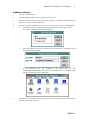
1
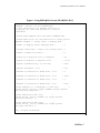
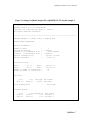
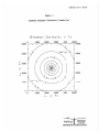
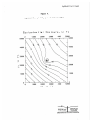
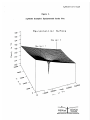
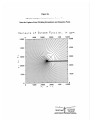
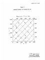
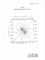
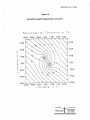
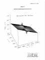
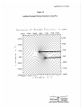
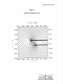
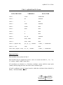
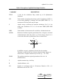
AqModel
for Windows™
Version 2.1 User’s Manual
Drawdown—Capture Zones—Flow Nets—Well Head Protection—Well Field Simulation
WellWare
™
1003 Prospect Hts
Santa Cruz, CA 95065
(408) 426-8260
Effective Software for Groundwater Prof
AqModel for Windows User's Manual
1
AqModel
™
Version 2.1 for Windows User's Manual
Contents
DISCLAIMER ............................................................................................................ 2
AqModel Requirements............................................................................................... 3
Software Installation.................................................................................................... 3
SURFER.......................................................................................................... 3
AqModel Installation ....................................................................................... 4
Diskette Files .............................................................................................................. 5
Quick Start .................................................................................................................. 6
AqModel ..................................................................................................................... 7
Drawdown and Potential Distribution .............................................................. 7
Pumping Near Hydrogeologic Boundaries ....................................................... 8
Stream Functions ............................................................................................. 8
Unconfined Aquifers........................................................................................ 9
Capture Zone Models....................................................................................... 9
Well Head Protection....................................................................................... 10
Data Input ................................................................................................................... 11
Running AqModel....................................................................................................... 12
Run Time Error Message ................................................................................. 13
Model Output Files...................................................................................................... 14
Model Graphics........................................................................................................... 14
Drawdown ....................................................................................................... 14
Equipotentials.................................................................................................. 14
Equipotential Surface....................................................................................... 15
Stream Functions ............................................................................................. 15
Flow Nets ........................................................................................................ 15
Example Problems....................................................................................................... 17
Example 1. Steady State, 1 Pumping Well ....................................................... 17
Example 2. Steady State, 1 Recharge Well....................................................... 19
Example 3. Transient, 1 Pumping Well. ........................................................... 19
Example 4. Transient, 1 Recharge Well. .......................................................... 19
Example 5. Steady State, 1 Pumping Well and 1 Recharge Well ...................... 19
Tips............................................................................................................................. 21
Acknowledgments....................................................................................................... 21
References................................................................................................................... 22
FIGURES
APPENDIX A—AqModel Data
APPENDIX B—Modeling Approaches for Hydraulic Control of Groundwater Contamination
WellWare
AqModel for Windows User's Manual
2
AqModel
™
Version 2.1 for Windows User's Manual
DISCLAIMER
WellWare and Gerald T. O'Neill make no representations or warranties with respect to the contents
hereof and specifically disclaim any implied warranties of fitness for any particular purpose. WellWare
and Gerald T. O’Neill will not be liable for any damages, losses, or claims consequent to use of this
software or the methods described herein. Further, WellWare and Gerald T. O'Neill reserve the right to
revise this publication and software, and to make changes from time to time in the content hereof without
obligation to notify any person of such revisions or changes.
Models are useful tools and it is the responsibility of the user of a model to correctly apply it in a
meaningful way.
Copyright © 1990–1993 by Gerald T. O'Neill.
All Rights Reserved.
No part of this manual may be reproduced or transmitted in any form or by any means, electronic or
mechanical, including photocopying, scanning, and recording, for any purpose other than the purchaser's
personal use, without the written permission of WellWare and Gerald T. O'Neill.
The software programs on the accompanying disk may not be copied, except to install on one computer
"hard disk" and for backup purposes only by the original purchaser.
WellWare
AqModel for Windows User's Manual
3
AqModel Requirements
• IBM-PC 386 SX or higher or 100% compatible microcomputer with hard disk drive,
MS-DOS® 5.0 or higher and Windows Version 3.1 or higher. Windows must be run
in 386 Enhanced Mode.
• Golden Software, Inc. SURFER® version 4 or higher and SURFER compatible
graphics adapter, monitor, and printer or plotter.
• A math coprocessor is used if present; however, it is not required.
Software Installation
SURFER
SURFER® is required for AqModel graphics on a PC. It is not included with AqModel
and can be purchased from Golden Software, Inc. by calling 1-800-333-1021 or 1-303279-1021. SURFER should be installed before using AqModel and must be available to
AqModel through the DOS PATH command. The following shows one way of correctly
configuring SURFER for use with AqModel.
•
Install SURFER in a directory called C:\SURFER.
•
Add SURFER to the PATH command in the AUTOEXEC.BAT file as follows:
PATH C:\;C:\DOS;C:\SURFER; etc.
•
Restart the computer.
•
At the DOS prompt, configure SURFER for your video hardware and output device
by typing the following commands:
PLOT/i Enter
This command will configure your output device (printer,
plotter, graphics file format) for use with SURFER.
VIEW/i Enter
This command will configure your video display for use
with SURFER.
WellWare
AqModel for Windows User's Manual
4
AqModel Installation
1.
Start Microsoft Windows.
2.
Insert the AqModel diskette into the appropriate drive A or B.
3.
Select Run from the Program Manager File menu and type A:INSTALL or B:INSTALL and
then press Enter or choose the OK button.
4.
INSTALL will copy AqModel files to your C: drive into a directory named C:\AQMODELW.
5.
-a-
Create a new group for AqModel in Program Manager; From the File menu, choose
New. The New Program Object dialog box appears.
-b-
Select the Program Group option, and then choose the OK button. The Program Group
Properties dialog box appears.
-c-
In the Description box, type AqModel. In the Group File box, type
C:\AQMODELW\AQMODEL and then choose the OK button. The AqModel Group
appears (the following view is maximized):
6.
Installation is now complete! We suggest that you review this User's Manual and the Example
Problems before using AqModel.
WellWare
AqModel for Windows User's Manual
5
Diskette Files
The following files are found on the accompanying diskette:
INSTALL.BAT
A batch file for installing AqModel on a hard disk.
DRAWDOWN.BAT
A batch file for running TOPO to plot drawdown.
EQUIPLOT.BAT
A batch file for running TOPO to plot equipotentials.
EQUISURF.BAT
A batch file for running SURF to plot equipotential
surface.
STREAMFN.BAT
A batch file for running TOPO to plot stream
functions.
FLOWNET.BAT
A batch file for creating and viewing flow nets.
DRAWDOWN.CMD
A TOPO command file for creating Drawdown contours.
EQUIPLOT.CMD
A TOPO command file for creating Equipotential
contours.
EQUISURF.CMD
A SURF command file for creating Equipotential surface
plots.
STREAMFN.CMD
A TOPO command file for creating Stream Function
contours.
EXAMPLE#.DAT
An AqModel example data set.
EXAMPLE#.TXT
Corresponding model output file for Example#.
AQMODELW.EXE
AqModel for Windows application program.
PREAQMW.EXE
Data preprocessor for AqModel for Windows.
UNITS.EXE
Units conversion program by HydroLink.
AQMODEL.IL
AqModel icon library.
AQMODEL.GRP
AqModel Program Manager group file.
WellWare
AqModel for Windows User's Manual
6
Quick Start
If you do not wish to read the manual at this time, and have already installed SURFER
and AqModel (see Software Installation), simply start Windows and then double-click on
the AqModel Program Group Icon in Program Manager to open the AqModel Group.
Then, simply double-click on the icon corresponding to the task you wish to perform:
Double-click Icon:
Description:
PREAQM
Create AqModel data files.
AqModel
Run AqModel.
UNITS
Make Units conversions.
Drawdown
Create a Drawdown contour plot.
Equipotentials
Create an Equipotential contour plot.
Equipotential Surface
Create an Equipotential Surface plot.
Stream Functions
Create a Stream Function contour plot.
Flow Net
Create a Flow Net plot.
WellWare
AqModel for Windows User's Manual
7
AqModel
AqModel (Aquifer Model) is a general aquifer modeling program for calculating
drawdown, potential distribution, and stream functions. Practical uses of the model
include well field simulation, flow net generation, and determination of capture zones of
single or multiple well recovery systems. AqModel is also useful for determining well
head protection areas.
AqModel is an analytical groundwater flow model which yields an exact solution to the
problem of wells pumping in a confined aquifer under uniform flow conditions
(homogeneous and isotropic transmissivity). AqModel is applicable to two-dimensional
uniform groundwater flows with multiple pumping and/or recharge wells.
Golden Software’s SURFER is required for AqModel graphics on a PC. AqModel
generates .GRD files in SURFER format and AqModel ships with preformatted
command files for controlling various aspects of graphics creation using SURFER’s
TOPO (contour maps) and SURF (3D surface plots) routines. These files make it easy to
run AqModel and create graphics with SURFER in the Windows environment. SURFER
supports a wide variety of graphics cards, monitors, printers (including PostScript®) and
plotters—and graphics formats including AutoCAD DXF™ and HPGL. Used in
conjunction with SURFER, AqModel is a powerful groundwater analytical and
presentation tool.
Drawdown and Potential Distribution
The head distribution for steady-state conditions is determined by superposition of
solutions for uniform flow and equilibrium drawdown (Thiem) by multiple wells:
N
hx,y = hp – i(xcos + ysin) –
QjlnRr
1
2T
j=1
where hx,y is the head at any point x,y in the aquifer, hp is the initial head at a point in
the aquifer, i is the hydraulic gradient and is the direction of uniform groundwater flow,
T is the aquifer transmissivity, Qj is the discharge (+) or recharge (–) rate at well j, N is
the number of wells, R is the radius of influence of the well and r is the radial distance
from the well to the point x,y.
AqModel assumes a default value for hp = 100 ft at the point x = 0, y = 0.
Numerical values of steady state drawdown calculated by AqModel should be taken as
approximate due to the difficulty in estimating a realistic value of R, the distance beyond
which drawdown is negligible. AqModel uses a default value of R = 20,000 ft. If the
distance between points XMIN, YMIN and XMAX, YMAX specified by the user is
greater than 20,000 ft, AqModel adds that distance to R. In effect, AqModel assumes the
distance to negligible steady state drawdown is beyond the limits of the model area. In
WellWare
AqModel for Windows User's Manual
8
the above equation, R > r, and since R appears as log R, even large errors in estimating R
do not appreciably affect the resulting drawdown calculations.
Because steady flow cannot exist in an infinite aquifer, the radius of influence is a
problematic term. The flow is unsteady, where a transient state describes the temporal
features of unsteady flow, until a recharge source is intercepted by the expanding cone of
depression. It is perhaps more constructive to think of R as being the distance at which
the aquifer head remains constant.
Although steady state and uniform flow conditions are not often met in the field, analyses
based on these assumptions are nevertheless practical and useful. It remains the
responsibility of the user of a model to correctly apply it in a meaningful way.
If a time dependent head distribution is desired, the solution is given by superposition of
solutions for uniform flow and transient drawdown (Theis) by multiple wells:
N
1
hx,y = hp – i(xcosa + ysina) –
Q W(u)
4T j
j=1
where
W ( u) = e y
dy
y
and
u=
r2 S
4Tt
W(u) is the so called "well function of u" and is calculated, for values of u, from a
polynomial approximation to the exponential integral written as an infinite series; y is a
dummy variable of integration, S is the storage coefficient and t is time.
Pumping Near Hydrogeologic Boundaries
The influence of hydrogeologic straight line boundaries can be approximately simulated
with AqModel using the method of images. A constant head boundary can be simulated
by using a line of recharge wells and a no flow boundary can be simulated using a line of
pumping wells. Refer to texts on groundwater hydrology for an explanation of the
method of images and its application (e.g., [Bear, 1979], [Freeze and Cherry, 1979]).
Stream Functions
Stream functions, denoted by the symbol , are functions that are everywhere tangent to
the specific discharge vector. Contours of the stream function are called streamlines. In
steady state flow, streamlines indicate the direction of flow at every point (see
WellWare
AqModel for Windows User's Manual
9
APPENDIX B). AqModel calculates stream functions for the model area by adding the
stream functions for uniform and radial flow:
1
= –Ki(ycos–xsin) +
2b
N
Qj tan-1yx
j=1
where K is the hydraulic conductivity and b is the aquifer thickness (see, e.g., McWhorter
and Sunada, [1977]).
Unconfined Aquifers
AqModel can be applied to unconfined aquifers where the drawdown is small in
comparison with the saturated aquifer thickness. For flow in unconfined aquifers that
satisfies this requirement, use T = Kb where b is the initial saturated aquifer thickness and
replace S with Sy (specific yield of unconfined aquifer) in the AqModel data set (see
APPENDIX A). This method makes use of the Dupuit assumptions and fails when vertical
flow components are significant. See Jacob [1950] for more information.
Capture Zone Models
AqModel facilitates determination of capture zones by calculating stream functions
which are then contoured using SURFER to show the streamlines or groundwater
pathlines. By definition, no flow crosses a streamline. The streamline that separates flow
to the well from that which passes the well is called the dividing streamline. Thus, the
dividing streamline outlines the capture zone. It may be determined by calculating the
stream function at sufficient density and shown by contouring the stream function at a
sufficiently small contour interval. An example of using AqModel to determine the
capture zone of a single pumping well is presented in detail in the section Example
Problems (see Example 1).
AqModel has been compared with other popular models for determining well capture
zones including RESSQ [Javandel et al., 1984] and PATH3D [Zheng, 1989]. The same
results were obtained for a problem common to AqModel, RESSQ, and PATH3D.
A good introductory note on modeling methods for hydraulic control of groundwater
pollution is given by O'Neill [1990]. This paper presents examples from AqModel,
RessqM (a modified version of RESSQ available from WellWare™), and PATH3D. A
copy of the paper is included in APPENDIX B.
AqModel is limited to determination of steady-state capture zones in uniform flows. To
determine the extent of capture at a given time in steady uniform flows, use RessqM by
WellWare [O'Neill, 1992]. For unsteady flows in non-homogeneous aquifers, use a
numerical groundwater flow modeling code (e.g., MODFLOW) and a particle tracking
code that works in concert with the flow model (e.g., PATH3D). An application of
numerical groundwater modeling and particle tracking to analyze remedial alternatives at
a Superfund site is presented by Zheng et al. [1991].
WellWare
AqModel for Windows User's Manual
10
Well Head Protection
AqModel is useful for determining well head protection areas. By using AqModel to
determine streamlines and capture zones, information is provided on critical areas of the
aquifer to protect because eventually the well will discharge water from these areas.
Of course, there is more to a well head protection program than determining groundwater
flow paths and this manual does not intend to address well head protection strategies.
Well construction, source identification and contaminant properties should be considered
as well as the overall management of the well field. But groundwater flow path
delineation is an important part and AqModel can provide some assistance where the
flows do not depart significantly from the assumptions of uniform, steady flow.
For more realistic modeling of groundwater flow paths in complex aquifers, refer to
Zheng [1989].
WellWare
AqModel for Windows User's Manual
11
Data Input
Input to AqModel consists of one data set. The data file may be created with conventional
text editors or word processing programs, or by using PREAQM, the preprocessor
provided with AqModel. To run PREAQM, simply double-click on its icon. Enter data by
typing responses to PREAQM prompts and then by pressing the Enter key. The
following figure shows part of the interactive PREAQM screen display with data from
EXAMPLE1.DAT. On-Line Help is available for the PREAQM Windows interface.
Select Index from the Help menu for a hypertext list of menu commands and procedures
for which help is available.
We suggest that you first use PREAQM to create a data set for an AqModel simulation.
Then, make edits to this data set using the Windows Notepad (or another text editor) as
required. The data file is simple to construct and edit (see Figure 1 and APPENDIX A).
The input data must be in the units and order specified in APPENDIX A. If you use a
word processor, remember to save the data file as "TEXT ONLY" because AqModel
cannot understand word processing control characters.
It is important to enter data in the units specified by PREAQM because units are
converted in the program. A supplementary program call UNITS is provided for units
conversions compliments of Milovan S. Beljin of HydroLink. Double-click on the
UNITS icon to start UNITS. The program is user friendly and self explanatory.
WellWare
AqModel for Windows User's Manual
12
Running AqModel
Double-click on the AqModel icon to run AqModel. AqModel will execute and ask you
to enter the name of the data file you created by using PREAQM (or a word processing
program). AqModel displays the input data on the computer screen (partly shown on the
following figure) before proceeding with the simulation. You can terminate the program
by pressing Ctrl+C or by selecting Exit from the File menu. On-Line Help is available for
the AqModel Windows interface. Select Index from the Help menu for a hypertext list of
menu commands and procedures for which help is available.
WellWare
AqModel for Windows User's Manual
13
While AqModel is executing, Running appears in the Status Bar. When AqModel is
completed, Finished appears in the Status Bar. Upon normal termination of AqModel, the
following message box appears:
Choose Yes to return to the Program Manager.
Choose No to return to AqModel if you wish to browse the AqModel window display
and/or select and copy output to a word processing program. Note that AqModel output is
automatically saved to a file named AQMODEL.TXT each time AqModel is run. You
can open and print this file from most any text or word processor including the Windows
Notepad.
Run Time Error Message
If you experience the following error message while running AqModel:
run-time error M6202: MATH
-log: SING error
Edit LINE 9 in the AqModel data set with an editor or word processing program. Change
the values of NX and NY (see APPENDIX A) by successively increasing both numbers
by 1 (from 61 = default) to 62, 63, ... and run AqModel again until you no longer get the
error. This error message occurs when a grid calculation point (or node) falls on a well
location. Changing the number of calculation points will also change their locations (and
therefore fix the error) without causing a loss in accuracy of the solution.
WellWare
AqModel for Windows User's Manual
14
Model Output Files
AqModel creates four output files for each model run during steady-state simulations.
The output files are deleted and replaced with new ones for each subsequent model run.
Therefore, be sure to rename output files that you wish to save by using the File Manager.
The output files are described in the following.
DRAWDOWN.GRD
area.
EQUIPLOT.GRD
STREAMFN.GRD
AQMODEL.TXT
– drawdown (ft) at each calculation node in the model
– hydraulic head (ft) at each calculation node.
– stream function (gpm) at each calculation node.
– listing of model data and drawdown at observation wells.
Note: If a transient simulation is requested (S is not equal to zero), then only the heads
and drawdown are calculated and STREAMFN.GRD is not obtained. This is
because stream functions are not defined in unsteady flows.
A listing of AQMODEL.TXT for EXAMPLE1.DAT is shown on Figure 2.
Model Graphics
Each .GRD file can be read directly by Golden Software's SURFER to contour the heads,
drawdown, and stream functions. Although WellWare assumes that users are familiar
with SURFER, preformatted SURFER command files (.CMD) are provided with
AqModel to make creating graphics an easy and effective process for the novice as well
as the experienced SURFER user. To create .PLT files and print or plot graphics from
SURFER, go to TOPO's or SURF's Output menu and select Send plot to installed output
device and press Enter.
Examples of AqModel graphics are shown on the Figures and are presented in the section
Example Problems. The various types of AqModel graphics are discussed below.
Drawdown
Double-click on the icon labeled Drawdown to create a contour plot of drawdown from
the most recent AqModel run. SURFER's TOPO program is executed in Full-Screen
mode. When the TOPO menu appears, press the F2 key to view the graphics. When
finished, press ESC and Enter to return to Windows. Figure 3 shows a drawdown
contour plot from Example 1.
Equipotentials
Double-click on the icon labeled Equipotentials to create a contour plot of equipotentials
from the most recent AqModel run. TOPO is executed in Full-Screen mode. When the
TOPO menu appears, press the F2 key to view the graphics. When finished, press ESC
and Enter to return to Windows. Figure 4 shows an equipotential contour plot from
Example 1.
WellWare
AqModel for Windows User's Manual
15
Equipotential Surface
Double-click on the icon labeled Equipotential Surface to create a surface plot of
equipotentials from the most recent AqModel run. SURF is executed in Full-Screen
mode. When the SURF menu appears, press the F2 key to view the graphics. When
finished, press ESC andEnter to return to Windows. Figure 5 shows an equipotential
surface plot from Example 1.
Stream Functions
Double-click on the icon labeled Stream Functions to create a contour plot of stream
functions from the most recent AqModel run. TOPO is executed in Full-Screen mode.
When the TOPO menu appears, press the F2 key to view the graphics. When finished,
press ESC and Enter to return to Windows. Figure 6 shows a stream function contour
plot from Example 1.
Flow Nets
Double-click on the icon labeled Flow Net to create a flow net plot from the most recent
AqModel run. You must first create plot files for Equipotentials (EQUIPLOT.PLT) and
Stream Functions (STREAMFN.PLT) by double-clicking on their respective icons as
described above, and by creating the .PLT files from TOPO’s Output menu1. Make sure
this is done each time you want a flow net to ensure that old .PLT files are replaced with
the most recent AqModel results. Flow Net appends STREAMFN.PLT to
EQUIPLOT.PLT to create a new file called FLOWNET.PLT and then executes
SURFER’s VIEW in Full-Screen mode. VIEW automatically draws the flow net on the
screen. When finished, press the ESC key, select Quit from the menu and press Enter
to return to Windows. Note that VIEW is useful for viewing .PLT files.
Figure 7 shows the flow net from Example 1 obtained by combining the plots of Figure 4
and Figure 6.
AqModel can also create flow nets for the steady state case when there are no wells
pumping. Simply specify NW = 0, or set Q = 0 for each pumping or recharge well in an
existing data set (see APPENDIX A). There will be no drawdown and the equipotentials
and stream functions may be combined to create a flow net which shows the regional
aquifer flow due to hydraulic gradient and transmissivity alone. This type of plot (as
shown on Figure 8 from Example 1) may be useful to depict the amount of groundwater
flow passing a given boundary drawn on a map that the flow net is superimposed on. The
flow across the boundary is obtained by simply counting the number of streamlines that
cross the boundary and multiplying by the constant contour interval.
1See
Model Graphics.
WellWare
AqModel for Windows User's Manual
16
The traditional graphical method of constructing flow nets emphasizes drawing
curvilinear squares throughout the region. Then, the discharge through any part of the
streamtube is calculated from the flow in one element. By contouring the stream function
at a constant interval, the discharge through each streamtube is the same. Obtaining
perfect curvilinear squares is not essential to drawing flow nets with AqModel as long as
a constant known contour interval is used to draw the streamlines. Admittedly, the flow
net elements on Figures 7 and 8 are somewhat rectangular rather than perfectly square.
But this does not diminish the utility of these plots in the slightest. However, it is also
true that square elements are more attractive. The “squareness” can be improved by
selecting appropriate contour intervals for both the equipotential and stream function
plots.
WellWare
AqModel for Windows User's Manual
17
Example Problems
Data sets for the following example problems are provided on the accompanying disk.
These are intended as an introduction to using AqModel. Example 1 and Example 5 will
be presented in some detail in the following. Users are encouraged to run these problems
and experiment with the data sets.
Example 1. Steady State, 1 Pumping Well
This problem involves a single pumping well in uniform flow. The problem is to
determine the distribution of drawdown and water levels in the aquifer. In addition, we
desire a plot of the groundwater pathlines and a flow net. And we want to know the
location of the capture zone. As demonstrated in the following, AqModel easily provides
solutions to each of these tasks.
The data set EXAMPLE1.DAT and the output shown on Figures 1 through 6 were
generated by using PREAQM and AqModel as discussed previously. AqModel output is
listed on Figure 2 and in the diskette file EXAMPLE1.TXT.
Figure 3 shows a contour plot of Drawdown from Example 1. Drawdown is concentric
around the pumping well located at the center of the plot. The contour interval is 0.5 ft.
Note that the “Observation Wells” are located between the 2.5 and 3 ft contours—the
drawdown shown on Figure 2 is 2.75 ft. Since both wells are equidistant from the
pumping well, they have the same drawdown.
Figure 4 shows a contour plot of Equipotentials from Example 1. AqModel assumes an
initially planar water table or equipotential surface with an aquifer reference head of 100
ft at the point x = 0, y = 0. The direction of groundwater flow is 45 degrees measured
counterclockwise from the positive X-axis; water level elevations decline in this direction
according to the hydraulic gradient of 0.002 ft/ft or about 10 ft/mile. The drawdown
produced by the single pumping well is added to the water level decline by uniform
groundwater flow to determine the head at each node.
Figure 5 shows a surface plot of Equipotentials from Example 1. This type of plot is
useful for showing the features of the equipotential surface. However, note the illusion of
the great pumping depression; the vertical scale is about 300 times that of the horizontal.
If the vertical and horizontal scales were equal, the vertical axis would only be about 0.01
inches high. Of course, the vertical scale is self-consistent, so one can note the relative
differences in head (although it is difficult to judge actual elevations on this orthographic
projection).
Figure 6 shows a contour plot of Stream Functions from Example 1. Contours of the
stream function are called streamlines and they represent groundwater pathlines in steady
state flows. This plot shows the paths that groundwater will follow in this example. The
direction of flow is indicated by the arrows.
WellWare
AqModel for Windows User's Manual
18
AqModel determines the stream function throughout the model area in units of discharge
(gallons per minute or gpm) over the entire aquifer thickness. The pumping well
discharges at the rate of 200 gpm in this example, so if one counts the number of
streamlines intersecting the well and multiplies by the contour interval (20 gpm in this
case), one should get the discharge rate of the well. Note that there are, in fact, 10
streamlines intersecting the well. Similarly, the discharge between adjacent streamlines
(along a so-called streamtube) is obtained by subtracting their values and equals the
constant contour interval.
Note the thick line in the positive X-direction at the well (how could you miss it?). This
line is the result of a “bunching up” of contour lines due to the discontinuity in stream
functions at the well. This is a problem for us only because it blemishes an otherwise
beautiful plot. The simple solution is to ignore it if you can; it is not an error in the
model. However, the problem cannot be easily corrected because we’re using a
contouring program to draw streamlines. The plot on the cover of the manual once looked
like this but was then improved by a graphic artist who erased the thick line and
connected the streamlines. This is a good technique for final presentations. Another
suggestion is to increase the number of calculation points (NX and NY) which will result
in a thinner line (and also consume more disk space).
The capture zone of the single pumping well can be identified on this plot by contouring
the stream function at a sufficiently small interval. The capture zone (in two dimensions)
is the area of aquifer which contributes flow to the well. The capture zone can be defined
by the dividing streamline that separates flow to the well from that which passes the well.
The stream function was contoured at a 5 gpm interval to produce Figure 6b. Note the
velocity stagnation point downstream of the well. This point is located at the intersection
of the dividing streamline and a line in the direction of flow at a distance from the well
given by:
xs =
Q
2 bq
where q = Ki is the specific discharge. A quick hand calculation yields Xs = 610 ft
approximately. The scale on Figure 6b is 1 inch = 1250 ft. If we measure the distance
from the well to the stagnation point in inches and multiply by 1250, we find the distance
to be about 610 ft.
The width of the capture zone at the well measured along a line perpendicular to the
gradient vector is about 1.54 inches or 1925 ft. It is also determined by W = Q ÷ 2 Ti . Far
upstream from the well, the capture zone will be about 3850 ft wide. Javandel and Tsang
[1986] present useful solutions for dividing streamlines in uniform flow where the wells
are aligned perpendicular to the gradient vector.
Figure 7 shows the flow net from Example 1 obtained by combining the plots of Figures
4 and 6 by double-clicking on the Flow Net icon as described in the section Flow Nets.
WellWare
AqModel for Windows User's Manual
19
Figure 8 shows a flow net for Example 1 with no pumping wells. The stream function is
contoured from –183.65 to 183.65 gpm in 40 gpm intervals. The total flow across the
diagonal width of the modeled area is Q = TiW (Darcy’s Law) = 367.3 gpm = 183.65*2.
Of course, you don’t need to draw a flow net to determine the discharge across a line
perpendicular to the gradient in steady, uniform flow. But the plot makes it easy to depict
the flow.
Example 2. Steady State, 1 Recharge Well.
This is a steady state problem identical to Example 1 except that the well is now a
recharge well. AqModel output is listed in EXAMPLE2.TXT. Users are encouraged to
run the example problem and plot the results. What does a negative value for drawdown
mean? How do the equipotential and streamline patterns differ from the case where the
well is pumping? What if the direction of flow were 225 degrees in this example?
Example 3. Transient, 1 Pumping Well.
This is a transient problem similar to Example 1. AqModel output is listed in
EXAMPLE3.TXT. Note that stream functions are not computed.
Example 4. Transient, 1 Recharge Well.
This is the equivalent of Example 3 where the well is now recharging. AqModel output is
listed in EXAMPLE4.TXT.
Example 5. Steady State, 1 Pumping Well and 1 Recharge Well
This is a steady state problem with 1 pumping well and 1 recharge well. This problem is
derived from Example 2 of Javandel et al. [1984, p.48] for the RESSQ model. AqModel
output is listed in EXAMPLE5.TXT.
Figure 9 shows contours of drawdown around the pumping and recharge wells. Note the
zero drawdown contour between the wells.
Figure 10 shows the equipotential pattern developed in the vicinity of the wells. Compare
this plot with those from Examples 1 and 2. Note that the flow direction here is also 45
degrees.
Figure 11 depicts the natural gradient and the effects of the buildup of head due to the
recharge well and the drawdown due to pumping.
Figure 12 shows the streamline pattern. Observe that water flows from the recharge well
to the pumping well. The contour interval is approximately 10 gpm. There are 9
streamlines “leaving” the recharge well that “arrive” at the pumping well. Therefore,
about 90 gpm of recharged water is ultimately pumped back out. Using RESSQ, Javandel
et al. [1984, p. 54] determined the approximate arrival times of water moving along the
streamlines from the recharge well to the pumping well. The range was from about 5 to
22 years.
WellWare
AqModel for Windows User's Manual
20
RESSQ has been described as being “user hostile”. O’Neill [1990, 1992] has modified
RESSQ to include a data preprocessor and to interface with SURFER for custom
graphics. This useful code, called RessqM, is now available. Contact WellWare for
more information.
Figure 13 shows a flow net plot for Example 5.
WellWare
AqModel for Windows User's Manual
21
Tips
COPY CENTERED.SYM from C:\SURFER to C:\AQMODELW if you plan to use
centered symbols to enhance your plots, post data, etc.
To create .PLT files and print or plot graphics from SURFER, go to TOPO's or SURF's
Output menu and select Send plot to installed output device and press Enter.
SURFER's VIEW program is useful for viewing .PLT files.
Acknowledgments
Gerald T. O'Neill is grateful to Dr. Chunmiao Zheng of S.S. Papadopulos & Associates,
Inc. for his assistance in writing the solution for handling the discontinuity in stream
functions at a well.
Gerald T. O'Neill is grateful to Milovan S. Beljin of HydroLink for the UNITS program.
DXF™ is a trademark of AutoDesk, Inc.
MS-DOS® is a registered trademark and Windows is a trademark of Microsoft
Corporation.
PostScript® is a registered trademark of Adobe Systems Incorporated.
SURFER® is a registered trademark of Golden Software, Inc., Golden, Colorado.
WellWare
AqModel for Windows User's Manual
22
References
Bear, J., 1979. Hydraulics of Groundwater. McGraw-Hill, Inc., New York, NY., 569p.
Freeze, R.A. and J.A. Cherry, 1979. Groundwater. Prentice-Hall, Englewood Cliffs,
N.J., 604p.
Jacob, C.E., 1950. Flow of Groundwater. Engineering Hydraulics, ed. H Rouse. John
Wiley and Sons, New York, pp. 321-386.
Javandel, I., Doughty, C., and C.F. Tsang, 1984. Groundwater Transport: Handbook of
Mathematical Models. AGU Water Resources Monograph 10. Washington, D.C.
228 p.
Javandel, I. and C.F. Tsang, 1986. Capture Zone Type Curves: A Tool for Aquifer
Cleanup. Ground Water, Vol. 24, No. 5, pp.616-625.
McWhorter, D.B. and D.K. Sunada, 1977. Ground-Water Hydrology and Hydraulics.
Water Resources Publications, Fort Collins, CO. 290p.
O'Neill, G.T., 1990. Modeling Approaches for Hydraulic Control of Groundwater
Contamination. Proc. Hazardous Materials Control Research Institute's HMC Great Lakes '90 Conference, Session on Contaminated Groundwater Control,
Sept. 26-28, 1990, Cleveland, Ohio. pp. 112-116.
O’Neill, G.T., 1992. RessqM User’s Manual. WellWare.
Zheng, C., 1989. PATH3D–A Ground-Water Path and Travel Time Simulator. User’s
Manual. S.S. Papadopulos & Associates, Inc. 7944 Wisconsin Avenue, Bethesda,
MD 20814.
Zheng, C., G.D. Bennett, and C.B. Andrews, 1991. Analysis of Ground-Water Remedial
Alternatives at a Superfund Site. Ground Water, Vol. 29, No. 6, pp.838–848.
WellWare
AqModel for Windows User's Manual
Figure 1. Using PREAQM to Create EXAMPLE1.DAT
PREAQM - Version 1.11 for Windows(TM)
A Data Preprocessor for AqModel Version 2.11
Copyright (C) 1990-1993 by Gerald T. O'Neill
WellWare
Please Enter AqModel Data File Name: EXAMPLE1.DAT
Please Enter Title for the Simulation in Single Quotes
'AqModel Example 1: Steady State, 1 Pumping Well'
Number of Pumping and/or Recharge Wells
= 1
Storage Coefficient - Input 0 for Steady State = 0
Number of Observation Wells
= 2
Direction of Regional Flow, in degrees
= 45
Hydraulic Gradient of Regional Flow
= 0.002
Aquifer Transmissivity, in ft^2/day
= 5000
Aquifer Thickness, in ft
= 100
Minimum X Coordinate of Model Area, in ft
= 0
Maximum X Coordinate of Model Area, in ft
= 5000
Minimum Y Coordinate of Model Area, in ft
= 0
Maximum Y Coordinate of Model Area, in ft
= 5000
Enter Pumping (+) or Recharge (-) Well Data
1
Enter QX(ft), QY(ft), Q(gpm), WLABEL (single quotes)
2500,2500,200,'Pump Well'
Enter Observation Well Data
1
Enter XO(ft), YO(ft), WLABEL (in single quotes)
1000,1000,'Obs Well 1'
Enter Observation Well Data
2
Enter XO(ft), YO(ft), WLABEL (in single quotes)
4000,4000,'Obs Well 2'
Stop - Program terminated.
WellWare
AqModel for Windows User's Manual
Figure 2. Listing of AqModel Output File (AQMODEL.TXT) From Example 1.
_______________________________________________________________________
AqModel Version 2.11 for Windows(TM)
Copyright (C) 1990-1993 by Gerald T. O'Neill.
All Rights Reserved. WellWare
________________________________________________________________________
AqModel Example 1: Steady State, 1 Pumping Well
STEADY STATE SIMULATION
Aquifer Parameters . . .
Number of Wells
Storage Coefficient
Direction of Groundwater Flow
Gradient of Groundwater Flow
Aquifer Transmissivity
Aquifer Thickness
=
=
=
=
=
=
1
.0000E+00
45.00 degrees
.2000E-02
5000.00 ft^2/day
100.00 ft
Calculation Grid . . .
Xmin =
.00 ft
Xmax
Ymin =
.00 ft
Ymax
Number of Nodes in X-direction
Number of Nodes in Y-direction
=
=
=
=
5000.00 ft
5000.00 ft
61
61
Well Data . . .
X-ft
2500.00
Y-ft
2500.00
Total Pumping Rate
Flow-gpm
200.00
=
Well Label
Pump Well
200.00 gpm
Drawdown Results . . .
X-ft
1000.00
4000.00
Y-ft Drawdown-ft
1000.00
2.75
4000.00
2.75
Well Label
Obs Well 1
Obs Well 2
WellWare
AqModel User's Guide
APPENDIX A
AqModel Data
WellWare
™
1003 Prospect Hts
Santa Cruz, CA 95065
(408) 426-8260
Effective Software for Groundwater Prof
AqModel User's Guide
Table 1. AqModel Data File Format
DATA FILE LINE
VARIABLE
DATA TYPE
LINE 1
TITLE
CHARACTER
LINE 2
NW
INTEGER
LINE 3
S
REAL
LINE 4
IOBS
INTEGER
LINE 5
ALPHA
REAL
LINE 6
GRAD
REAL
LINE 7
T
REAL
LINE 8
B
REAL
LINE 9
NX, NY
INTEGER
LINE 10
XMIN, XMAX
REAL
LINE 11
YMIN, YMAX
REAL
LINE 12 (Repeat NW)
QX, QY, Q, ‘WLABEL’
3 REAL, 1 ‘CHARACTER’
LINE 12 + NW
TIME
REAL
LAST LINE (Repeat IOBS)
XO, YO, ‘WLABEL’
2 REAL, 1 ‘CHARACTER’
Important Notes:
Data variables are described in Table 2.
Data variables may be separated by spaces, a tab, or a comma on LINE 9, 10, 11,
12 and the “LAST LINE” listed above.
All coordinates are absolute in a Cartesian coordinate system with the origin point
(XMIN,YMIN) being the lower left corner of the calculation grid.
All well coordinates (real and image) must be within the calculation limits defined by
XMIN, YMIN and XMAX, YMAX.
WellWare
™
1003 Prospect Hts
Santa Cruz, CA 95065
(408) 426-8260
Effective Software for Groundwater Prof
AqModel User's Guide
Table 2. Description of AqModel Data Input Variables.
VARIABLE
DESCRIPTION
TITLE
A title for the simulation. May contain up to 80 alphanumeric
characters.
NW
Total number of pumping and recharge wells in simulation. If NW = 0,
do not enter pumping or recharge well data (SKIP LINE 12). A
maximum of 501 total wells may be input.
S
Aquifer storage coefficient for transient simulations. Set S = 0 for
steady state simulations. If S = 0, do not enter TIME (SKIP LINE
12+NW).
IOBS
Total number of observation wells at which to calculate drawdown.
ALPHA
Direction of uniform regional groundwater flow, in degrees, measured
counterclockwise from the positive (+) X-axis being 0 degrees to a
vector in the direction of groundwater flow as shown below.
90
135.00°
180
0 (360)
270
If ALPHA is negative, AqModel will add 360 to the number.
Therefore, to specify flow in a clockwise direction from 0 degrees as
shown above, a negative number may be used (e.g., –20 = 340).
GRAD
The gradient of uniform regional groundwater flow, in ft / ft
(dimensionless).
T
Aquifer transmissivity, in ft2/day.
B
Aquifer thickness, in ft.
NX
Number of calculation nodes in X-direction. Default is NX = 61.
Maximum value of NX = 101.
WellWare
™
1003 Prospect Hts
Santa Cruz, CA 95065
(408) 426-8260
Effective Software for Groundwater Prof
AqModel User's Guide
NY
Number of calculation nodes in Y-direction. Default is NY = 61.
Maximum value of NY = 101.
XMIN
Minimum value of X-coordinate of model area, in ft.
XMAX
Maximum value of X-coordinate of model area, in ft.
YMIN
Minimum value of Y-coordinate of model area, in ft.
YMAX
Maximum value of Y-coordinate of model area, in ft.
QX
The X-coordinate of a pumping or recharge well, in ft.
QY
The Y-coordinate of a pumping or recharge well, in ft.
Q
The (+) pumping or (–) recharge rate of a well, in gpm.
WLABEL
A label for each pumping or recharge well. May contain up to 10
characters that must be enclosed in ‘single quotes’.
TIME
Time of transient simulation, in days. SKIP THIS LINE IF S = 0.
XO
The X-coordinate of an observation well, in ft.
YO
The Y-coordinate of an observation well, in ft.
WLABEL
A label for each observation well. May contain up to 10 characters that
must be enclosed in ‘single quotes’.
WellWare
™
1003 Prospect Hts
Santa Cruz, CA 95065
(408) 426-8260
Effective Software for Groundwater Prof
AqModel User's Guide
APPENDIX B
Modeling Approaches for Hydraulic Control of Groundwater Contamination
by
Gerald T. O’Neill
WellWare™
Note: WellWare was formerly Software Solutions for Groundwater Hydrologists
WellWare
™
1003 Prospect Hts
Santa Cruz, CA 95065
(408) 426-8260
Effective Software for Groundwater Prof
AqModel User's Guide
WellWare
™
1003 Prospect Hts
Santa Cruz, CA 95065
(408) 426-8260
Effective Software for Groundwater Prof


![RessqM, Enhanced Version of RESSQ [Javandel et al., 1984]](http://vs1.manualzilla.com/store/data/005674408_1-e8a4b9f66c80cdc83d847a710e5b4b1f-150x150.png)