1
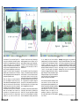
Geometric
and
algebraic
modelling
with
dynamic
geometry
software
Figure 1
The Geometer’s
Sketchpad V.4
and Cabri
Geometry II plus
With an image on the clipboard, use Edit and Paste
Picture to place the image on the current drawing.
Here, in Figure 2, I have pasted it twice in different
places to show how Sketchpad always treats this as
`transparent images’ so that construction lines are
not obscured by the image.
We will try to model the trajectory of the water
spout using a quadratic function of the form:
y = ax 2. Using the Graph menu we can define a
New Parameter – here called a 1 and then use Plot
New Function to define and plot a function
entered algebraically.
A particularly interesting form of modelling
became available in Sketchpad V.2 by being able to
import a picture via the Windows clipboard and to
superimpose constructions, axes and graphs on it.
This was not, to my knowledge, possible in Cabri 2.
The segment AC is drawn to define the direction of
the x-axis.
The function is entered as ‘a 1*x^2’. Sketchpad gives
it the label ‘f(x)’ and tidies up the algebraic
notation, as well as plotting the graph of the
function against our current axes.
When Sketchpad V.4 appeared it made algebraic
functions directly definable and plottable, thus
combining the features of dynamic geometry
software with those of a familiar graph-plotting
package. In particular we could now model
captured images either geometrically or
algebraically or both.
A point O is chosen on one of the images so as the
origin for coordinates, and lines drawn through O,
parallel and perpendicular to AC.
Adrian Oldknow
The flood gates opened for modelling with
dynamic geometry software (DGS) when both
Cabri II and Sketchpad V.2 allowed you to perform
calculations on measurements and to use such
results to plot the coordinates of a point
on specified axes. Using a subset of the x-axis as
the domain for a free (draggable) point P allowed
you perform calculations on its x-coordinate to
obtain a corresponding y-coordinate from some
function defined by the calculation. The resulting
point Q (x,y) would then trace a curve as P was
dragged on its domain – and that point could be
selected to leave a trace. Alternatively, the locus of
Q as a function of P could be drawn – the locus
being the graph of the function of x – which
never appeared explicitly in symbolic form
in the process.
16
Figure 2
I now illustrate an approach to algebraic modelling
applied to a digital photograph of the fountain in
Singapore harbour using Sketchpad V. 4 (see Fig 1).
A point B on it is used as a `slider’ so that AB
defines the unit distance for both axes.
The circle centre O, radius AB, is drawn (not
shown) and used to define the unit circle for a new
set of axes. The intersections of the circle with the
positive axes are shown as Px and Py.
The unit circle and the horizontal and vertical lines
are now hidden leaving only the axes.
By highlighting the parameter you can use the `+’
and ‘-‘ keys to increase or decrease its value.
I have also constructed a subset of the x-axis as the
domain of the sliding point P and illustrated the
“old” technique to obtain the dependent point Q
which can now be seen to trace the curve. If we
knew that a quadratic curve was also a parabola
with a `focus-directrix’ definition, we could have
imposed a geometric model by chosing some point
F on the negative y-axis as focus and drawn the
directrix as the line parallel to the x-axis through
17
Figure 3
the reflection of F in the x-axis (see Figure 3). If R
is any point on the directrix, we seek to construct
the point S on the perpendicular to the directrix at
R which is such that FS = SR. This means that
triangle FSR is isosceles and hence the vertex S is
the point where the perpendicular bisector of the
base FR meets the perpendicular to the directrix
through R. The locus of S with R is the geometric
parabola, and we can slide the focus F to discover
when it best agrees with both the water spout and
the algebraic (quadratic) model.
When Cabri Geometry II plus came out early this
year I was delighted to receive an early copy.
Certain features had immediate appeal, such as the
larger icons and menus which are more friendly
for whole class work, such as with an interactive
whiteboard. The major drawback is that the little
User Manual does not give much information
about the new features. One of these is the
introduction of the Expression option which
allows you enter a function of x using the same
notations as you would use with built-in
18
Calculator. I haven’t found a way of introducing a
variable parameter into such a function, but it is
easily editable to change any part of the equation.
To evaluate it, using the Evaluate an Expression
command, you must also specify a value to
substitute for x.
So in the model at the top of the next page (see
Figure 4), I have started in exactly the same way
as with Sketchpad – but the trick was to discover
how to import a picture! You do this by rightclicking the mouse anywhere on the background
and selecting Background Image, and the From
File – which allows you to import an image file
such as JPEG. You can also define a point with the
Point tool and right-click on it to import an image
which is draggable around the screen.
Just as before, the axes have been defined relative
to the origin O and unit points X,Y defined by the
slider B on AC. Now you need to define a variable
point Px on the x-axis and Measure its coordinates
(which I’ve labelled as Px) so that you have a value
Figure 4
of x to substitute into the function definition
(labelled here as f(x)), which returns a value which
I’ve labelled as Py. Use the Measurement Transfer
command to transfer this to the y-axis. Then
construct perpendiculars to the axes at Px and Py to
define their intersection as the point P. The locus of
P with Px is then the graph of the algebraic
function f(x). Dragging Px shows that P traces the
graph. Editing the function immediately changes
the shape of the graph. In Figure 4, the screen shot
from Cabri Geometry II plus, I have also shown the
geometric construction for the parabola.
So the moral of this little tale is that both the most
recent version of the two most widely used
dynamic geometry software packages allow you to
perform both geometric and algebraic modelling
using captured images. Perhaps Sketchpad has a
slight edge with its Plot As (x,y) and New
Parameter functions, but maybe Cabri has
something up its sleeve too – my final Sketchpad
file for the model weighs in at 3834 Kb against
Cabri’s 319 Kb.
Postscript: some people are very attached to
using the Numerical Edit feature of Cabri to enter
an initial value or parameter which can be easily
incremented, decremented or animated. The New
Parameter function of Sketchpad V. 4 allows just the
same strategy to be used – but with the added
advantage that units such as centimetres and
degrees can also be attached.
Adrian Oldkno w t.
Acknowledgement
Philip Yorke of Chartwell Yorke for providing the review copy of Cabri Geometry II plus .
19