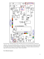
1
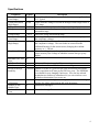
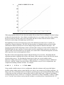
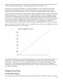
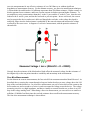
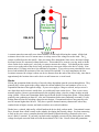
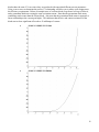
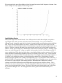
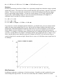
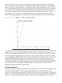
Curve Tracer
User Manual and Technical Specification
By Duane Becker 2005
INTRODUCTION.................................................................................................................................................................3
DESCRIPTION.....................................................................................................................................................................3
SPECIFICATIONS ...............................................................................................................................................................4
MAIN MENU ........................................................................................................................................................................5
TEST PROFILE SELECTION LINE .................................................................................................................................................5
ERASE USER TEST LINE ............................................................................................................................................................6
EDIT USER TEST LINE...............................................................................................................................................................6
SEND USER TEST LINE ..............................................................................................................................................................8
TEST DESTINATION NUMBER LINE ............................................................................................................................................8
TEST DESTINATION NAME LINE ................................................................................................................................................8
EXECUTE AND VIEW TEST RESULTS LINE ..................................................................................................................................9
VIEW DESTINATION TEST LINE .................................................................................................................................................9
V:I Viewer ..........................................................................................................................................................................9
I:V Viewer ........................................................................................................................................................................10
Test Data Text Viewer ......................................................................................................................................................10
SEND DESTINATION TEST LINE ...............................................................................................................................................10
ERASE DESTINATION TEST LINE..............................................................................................................................................11
RUN CALIBRATION LINE .........................................................................................................................................................11
The Calibration Sequence.................................................................................................................................................12
Quick Verification of Calibration .....................................................................................................................................13
CURRENT SOURCE UTILITY.....................................................................................................................................................13
TOGGLE TRUEZERO LINE ........................................................................................................................................................14
HIGH RANGE LINEARITY.........................................................................................................................................................14
USING THE CURVE TRACER.........................................................................................................................................16
TWO-WIRE MEASUREMENTS...................................................................................................................................................16
FOUR-WIRE MEASUREMENTS..................................................................................................................................................17
DIODES ..................................................................................................................................................................................18
LIGHT EMITTING DIODES........................................................................................................................................................20
RESISTORS .............................................................................................................................................................................22
WIRE RESISTANCE..................................................................................................................................................................22
TECHNICAL ASPECTS ....................................................................................................................................................23
2
Introduction
This curve tracer is designed to characterize any two-terminal device using a current excitation of up to
2.55 Amperes and a maximum voltage measurement of up to 8.190 volts. Its primary use is to characterize
diodes, LEDs, bridge rectifiers, and low-Ohm valued resistors. An EEPROM is used to hold up to ten
different test results, and up to ten different user test profiles, and retains the data even when the unit is
powered off. The user can edit the ten different user-test profiles for special tests not covered by the built
in test profiles. Each test current in a test is applied, and the resulting voltage developed by the device
under test is measured and saved to the selected test result file in EEPROM. The user can view any test
result as a voltage-versus-current or current-versus-voltage graph on the graphic LCD display, or see the
raw data as a list. User test profiles and test results can be exported through the RS232 serial port. A full
test of 251 test points takes only a quarter second to complete, so that the device under test won’t
appreciably heat up. The voltage measurement is accurate to +/- one millivolt, from 0.000 to 8.190 volts
with one millivolt resolution.
Description
The curve tracer has a graphic LCD display sporting text and graphics capability. A 16-button keyboard
provides the user interface for controlling the curve tracer and editing tests and data. A 9-pin serial RS232
port is available on the back for exporting data at 9600 baud, 8-bits, no parity, and one stop bit. Four-wire
Kelvin measurements are made via the four binding jacks on the front panel of the unit. Two of the posts
loop the current and are labeled I- and I+, and are black and red respectively. Conventional current
(positive current) comes out of the I+ binding post, and is to be returned into the I- post. The voltage
sensing posts are labeled S- and S+, are also black and red respectively, and are connected to the device
under test to measure the developed voltage during the tests. Normally, the current source post I+ and S+
positive Voltage sense (red colored) posts are shunted. The current return post I- and the -Voltage sense
(black colored) posts are also normally shunted. They may be unshunted for remote device or high current
testing. A pair of double banana plugs are provided for easy shunting of the posts.
A main menu provides access to all the functions, including built-in calibration procedures. This curve
tracer provides a fast, convenient means of characterizing all manner of two terminal devices. The primary
use is to characterize rectifiers, diodes, and diode bridges for voltage-current relationships. It is also useful
for measuring small-valued resistors to milliohm precision.
3
Specifications
Parameter
Current Resolution
(Low Range)
Current Resolution
(High Range)
Voltage Resolution
Voltage Accuracy
Typical
100 µA
Description
Finest allowable change in current on the low current range from 0 to
25.5 Typical
10 mA
Finest allowable change in current on the high current range from 0 to
2.55 Amps
1 mV
Finest measurable resolution of voltage measuring subsystem
+/- 1 mV Absolute accuracy of voltage measuring subsystem over the entire
measurable range.
Voltage Range
8.190 V
Full Scale voltage measurement range
Current Accuracy
+/- 20 µA Accuracy of delivered current for any value on the low range (up to
the compliance voltage).
(Low Range)
Current Accuracy
+/- 2 mA Accuracy of delivered current for any value on the high range (up to
(High Range)
the compliance voltage). The test results are corrected to the
calibrated linearity for the current source, bringing the resultant
accuracy to +/- 200 uA.
Compliance Voltage 9 V
Maximum voltage that can be applied while holding the current
source accuracy (the Voltage at which the current can’t go up any
higher)
Maximum User Test 507
Steps
Test Time Per Step 1 ms
500 µs stabilization time, plus 500 µs measuring time
Idle Current
0.12 A
Current drawn from wall outlet when not running a test.
EEPROM storage
1,000,000 Number of writes to a given 64-byte page in EEPROM for lifetime.
durability
This is equivalent to 68 tests per day for forty years. The EEPROM
is socketted for easy changing if necessary. Also, the last selected
destination test location is remembered so you can switch to a new
default test destination if one wears out.
Calibration
3
One potentiometer for high current range, one for low current range,
Adjustments
and one for voltage measurement full-scale adjustment.
Number of user10
Numbered 0 through 9
editable Tests
Number of Built-in
26
Lettered A through Z
Tests
4
Main Menu
The main menu is presented when the curve tracer is turned on. Each line describes the feature available
on that line. A line pointer “>“ is shown to the left side of the selected line, and is positioned initially at the
top line.
>TEST PROFILE LIN___5M ----- A
ERASE USER TEST PROFILE
EDIT USER TEST PROFILE
SEND USER TEST PROFILE TO HOST
TEST DESTINATION NUMBER ----- 0
TEST DESTINATION NAME YOURTEST
EXECUTE AND VIEW TEST RESULTS
VIEW DESTINATION TEST
SEND DESTINATION TEST TO HOST
ERASE DESTINATION TEST
RUN CALIBRATION PROCEDURE
CURRENT SOURCE UTILITY
TOGGLE TRUEZERO
OFF
HIGH RANGE LINEARITY
Use the up and down arrow keys on the keyboard to move the “>“ cursor to point to the feature line
desired.
Test Profile Selection Line
When this line is selected with the “>“ cursor, you may use the left and right arrow keys to increment or
decrement the test profile selection. Test selection numbers “0” up to “9” are user profiles, which may be
edited and saved through the Edit User Test Profile option. Test selection letters “A” up to “Z” are built in
test profiles, suitable for almost all your curve tracing needs. When you change the test profile selection,
the name is copied into the Test Destination Name line. When a test is run, the test results are stored in the
test destination number with the name indicated in the Test Destination Name line. You can change the
test destination number and name as you see fit before running the test. The keyboard is typomatic,
allowing you to hold down a key to scroll through the test selections.
The built in tests are described here.
Test Name
LIN___5M
LIN__10M
LIN__15M
LIN__20M
LIN__25M
LIN__30M
LIN__40M
LIN__50M
LIN__70M
LIN_100M
LIN_150M
LIN_200M
Description
Linear current sweep from 0 to 5 mA by 0.1 mA (51 points)
Linear current sweep from 0 to 10 mA by 0.1 mA (101 points)
Linear current sweep from 0 to 15 mA by 0.1 mA (151 points)
Linear current sweep from 0 to 20 mA by 0.1 mA (201 points)
Linear current sweep from 0 to 25 mA by 0.1 mA (251 points)
Current sweep from 0 to 30 mA
Current sweep from 0 to 40 mA
Current sweep from 0 to 50 mA
Current sweep from 0 to 70 mA
Current sweep from 0 to 100 mA
Current sweep from 0 to 150 mA
Current sweep from 0 to 200 mA
5
LIN_250M
LIN_300M
LIN_400M
LIN_500M
LIN_750M
LIN_1000
LIN_1500
LIN_2000
LIN_2500
LIN_2550
500_MAMP
1000_MA
2000_MA
2500_MA
Current sweep from 0 to 250 mA
Current sweep from 0 to 300 mA
Current sweep from 0 to 400 mA
Current sweep from 0 to 500 mA
Current sweep from 0 to 750 mA
Current sweep from 0 to 1000 mA
Current sweep from 0 to 1500 mA
Current sweep from 0 to 2000 mA
Current sweep from 0 to 2500 mA
Current sweep from 0 to 2550 mA
0 milliamps, then 500 milliamps constant for 10 tests
0 milliamps, then 1000 milliamps constant for 10 tests
0 milliamps, then 2000 milliamps constant for 10 tests
0 milliamps, then 2500 milliamps constant for 10 tests
For all currents at and less than 25.5 milliamps, the resolution in the current source is 0.1 mA. Once the
current being applied goes above this, it snaps to the nearest 10 mA resolution. Tests above 25.5 mA
generally don’t use the finest resolution for values below 30 mA, since the data is too fine to plot on the
graphs anyway. The accuracy of the high range current source is corrected through a linearity table. This
ensures that the current values reported for 30 mA and higher truly reflect what the curve tracer is
applying.
Erase User Test Line
When you have selected this line, and a user test profile from 0 to 9 is selected, you may type the “Y” yes
key to erase the selected user test profile. You are given a confirmation screen and are instructed to type
the UP arrow key to confirm erasing the user test. If a built in profile from A to Z is selected, this erase
feature is deactivated. You cannot erase a built-in test. When a user profile is erased, its name is changed
to “________”, eight underscores. The entire test is also erased to all zero current and no test steps.
Underscores are used since they sit right between the upper case ASCII letters and the lower case ASCII
letters, providing easy access to mixed case names if you edit the name of the user test.
Edit User Test Line
When you have selected this line, and a user test profile from 0 to 9 is selected, you may type the “Y” yes
key to start the user test profile editor. This editor allows you to change the name of the user test profile,
and to specify up to 507 test currents in any order. When the test editor is started the top line is presented
with the name of the test and the number of test steps in the test.
TESTNAME
STEPS=000
You use the up and down arrow keys to scroll through the test. The test steps are below the name line and
are numbered from 001 up to 507. On any test step line (that shows the number and current to be
applied), you may type the left arrow to indicate this is the last desired step in the test. If you type the left
arrow key on a numbered line, you are asked “OK TO CLEAR TO END OF FILE?” to confirm that you
want to erase all test points that follow the one currently displayed. This means that all test steps AFTER
the current one is going to be cleared to zero current and removed from the test sequence. Type the “Y”
key to confirm the Clear to End Of File of file. Any other key aborts the clear to end feature. A test step
is shown like this:
6
001
0.0000 AMPS
To edit a test name or test step, you must open it with the “Y” yes key.
When the test name line is opened, a block cursor is positioned under the first character of the name.
TESTNAME
n
STEPS=000
You may use the cursor left and right arrows to move the cursor. Use the up and down arrow keys to
change the selected character by scrolling through the full ASCII character set. Remember that the
keyboard is typomatic, and you may push and hold the up or down arrow keys to quickly scroll through
the characters. Set the characters as desired and use the left and right arrows to move the cursor left and
right for each character to be changed. If you plan to export user test profiles, be sure to set the name to a
valid DOS filename with no blanks. Underscores are fine for DOS filenames. When you have finished
changing the name, type the “Y” key to lock in the name and store it in memory.
When a test step line is opened with the “Y” key, a block cursor is positioned under the first digit in the
AMPS value.
001
0.0000 AMPS
n
The amperage to be delivered in that step is represented as X.XXXX AMPS. The values allowed in a test
step are 0.0000 AMPS up to 0.0255 in 0.0001 in 0.0001 Amp resolution. Above that, values from 0.0300
up to 2.550 AMPS are allowed in 0.010 Amp resolution. You may type in the digits for the desired
current, and the cursor automatically moves to the next character. You may also use the left and right
arrow keys to move the cursor (useful for backspacing when you’ve typed the wrong number). When
you’ve finished entering your value, type the “Y” key to lock in the value. If you type a value greater than
2.550 Amps, it is changed down to 2.550 AMPS. If you type a value that is overspecified for resolution
(like 1.234 AMPS), it is rounded to the nearest value (like 1.230 AMPS). Once you have typed the “Y”
key and the cursor turns off, you may scroll to another step, back to the name line (at the top), use the left
arrow key to erase to end of test, or type the “N” key to exit the test editor.
Anytime you are presented with the user test name line, the entire test file is reexamined and counted to
ensure that the number of steps shown is accurate. This is a good way to ensure that you have the correct
number of steps entered. The count is set to the last nonzero current value entry in the list. Ending a test
with a zero current value entry is not allowed. Generally you should enter amperage values that increase
or decrease in value, although you may enter any values that you desire or need.
When you are done changing the user test profile, type the “N” key to exit the test editor. The number of
steps to the last nonzero test current is counted up and saved in the file.
Note that if you specify a single current value in a test, and try to view the graph of the results, a single
point will be plotted that might be difficult to find on the graph. All the built-in tests include a starting
measurement of zero current, producing a smooth plot that starts at 0,0. If you want to more easily find
your specific test point on the graph, be sure to include your own starting zero current test point for the
first test point. The graphic viewers join successive points with straight lines, so it will be easy to find your
7
specific test point from the zero-zero point. The built-in single current value tests 500_MAMP,
1000__MA, 2000__MA, and 2500__MA all have a zero current test point at the start so a diagonal line is
drawn to the real test point on the graphs. You can always use the raw data text mode viewer to examine
specific test points to get the full data from them, regardless of where in the test they occur. Since the
graphing algorithm plots from the first test entry to the last, if you bounce around in the amperage domain,
going up and going down in amperage during the test, straight lines will interconnect those points,
producing a less than desirable graph. Normally, you would select the lowest currents and sweep upwards
to higher currents, and then end the test.
Send User Test Line
This feature is used to export a user test profile to a host computer. The serial protocol is RS-232
standard, 9600 baud, 8-bits, no-parity, one stop bit, with byte-for-byte acknowledge. The data that is sent
is the entire 1024-byte record for the user test profile selected in the Test Profile line. If you have a built-in
test profile selected, this feature is disabled and nothing will happen. User test profiles are numbered from
0 to 9. Each byte in the test profile is sent with full handshake. This means that the curve tracer sends out
the first character, and awaits any returned character in response from the host. After all 1024 bytes are
sent and acknowledged, the send profile feature completes. If a transmission error stops transmission, you
may type any key to abort the transmission. The format of the data bytes sent is:
Bytes
Bytes 0 and 1
Bytes 2 through 9
CurrentHi CurrentLo
Description
The high and low bytes respectively indicating the number of valid
testpoints in the record
The ASCII characters associated with the NAME for this user profile
---- 507 testpoint bytes-pairs follow ----Two bytes (MSB, LSB) that represent the current that would be applied for
this test step (in 100 microAmp units). E.G. 1.0000 Amps would be the
two bytes 27h and 10h since 2710h = 10000 decimal.
When you first type the “Y” key, you are prompted to get the destination host ready to accept data. The
destination host is responsible for receiving each byte and acknowledging each byte with any character in
return. A program CTDATA.EXE is available for handling profile and test result exporting from the curve
tracer. When the destination host is ready to receive and acknowledge the 1024 bytes, and is waiting on
the first byte, type the UP key on the curve tracer to start transmission. The operation takes a total of
about two seconds to complete. Even if your test profile does not have 507 test points, all data in the
record is transmitted. The host computer is responsible for ignoring any test points beyond the count
specified in the first two bytes.
Test Destination Number Line
When the “>“ cursor is pointing to this line, you may use the left and right arrow keys to select the
destination test number, from 0 to 9. This indicates which test results slot is used to store the test data
when it is run. Each test slot can hold a full test result and a test name. This test destination number is
stored in EEPROM and powers-up to the last selected destination number from the previous time you used
the curve tracer.
Test Destination Name Line
When the “>“ cursor is pointing to this line, you may type the “Y” key to edit the test destination name.
This name is filled in automatically anytime you switch test profiles or erase a test destination result. When
8
you type the “Y” key on this main menu feature, the screen is cleared and the current test destination name
is presented with a block cursor under the first letter.
RESULT01
n
You may then use the left and right arrow keys to move the cursor under the letter you want to change.
Use the up and down keys (with typomatic capability) to change each letter desired. The full ASCII set is
available. If you want to export test results to a PC, be sure to select a name that is a valid 8 character
DOS filename. When you are done editing the test destination name, type the “Y” again to return to the
main menu.
Execute And View Test Results Line
When the “>“ cursor is pointing to this line, and you type the “Y” key, the test profile selected at the top of
the screen is immediately run, and the results are stored in the destination test file selected. When the test
is completed, the test viewer is immediately started and shows the Voltage vs. Current graph. If the test
profile executed was an empty user profile, then there are no test results to view, and the curve tracer
simply beeps once to indicate that there was nothing to view. Read about the test viewer below. When at
least one test point is executed and saved in the test destination, you are launched into the test viewer.
When you exit from the test viewer using the “N” no key, you are returned to the main menu ready to run
the test again if desired. While in the test viewer, you may use the left and right arrow keys to select the
test display desired (V:I I:V or Testdata). The test results are stored in the EEPROM and are available for
viewing even when power has been cycled off and on again. Test results may be erased using the Erase
Destination Test feature.
View Destination Test Line
If you want to view a test already stored in the selected destination slot, put the “>” cursor on the View
Destination line, and type the “Y” key. If the test has no testpoints and is empty, the curve tracer will
simply beep to indicate that there are no test points available. If there are testpoints stored in the slot, they
are graphed on the default V:I graph, with voltage on the X axis, and current on the Y axis. When viewing
a test, you may use the left and right arrows to scroll through the three different viewing methods: V:I,
I:V, and Test Data Text. Typing the “N” key in any view will exit the viewer.
V:I Viewer
This view presents voltage on the X axis (left to right) and current on the Y axis (bottom to top). The axes
are scaled to fit the data, but are never scaled smaller than the smallest measurable resolution for the axis
parameter. That is to say, that the current axis will never be scaled smaller than 100 microamps per pixel,
and the Voltage axis will never be scaled smaller than 1 millivolt per pixel. The axes are scaled upwards if
necessary to fit the largest data point for that axis in the screen. The axes are also marked with a numbered
graticule to assist reading rough values from the screen. To exit any of the views, simply type the “N” key.
If you were to run a test expecting 0.250 Amps and 5.000 volts to show up on the graph, as you might for
example, if you ran a 20-Ohm resistor, sometimes the 5 Volt graticule might not show up. This is because
the highest voltage read during the test was less than 5 volts, perhaps 4.998 Volts. Since 5 Volts was not
in the test results, it was not shown on the graph. If you want to be absolutely sure that the 5 Volt
graticule is displayed in this example, consider using the next higher current excitation test or add one more
slightly higher excitation current to the test to ensure that the highest test goes beyond the 5 Volt result.
9
I:V Viewer
This view presents current on the X axis (left to right) and Voltage on the Y axis (bottom to top). The
values are scaled to fit the window, and the axes are numbered and have a graticule applied as well. Use
the left or right keys to switch to a different viewer, or the “N” key to exit the viewer.
Test Data Text Viewer
The test data text viewer presents the test data on one line that may be scrolled up and down. The very
top line shows the test name and the number of test steps in the test. Scrolling down, you will find
sequentially numbered test steps that show the test number, the current delivered in Amps, and the voltage
measured in Volts. For example:
YOURNAME
123
STEPS=329
1.2300-A
789=PGUP
123=PGDN
4.123-V
<-VIEWS->
N=EXIT
0=HOME
Use the up and down arrow keys to scroll through the data one line at a time. The keyboard has typomatic
action, so you can push and hold the up or down key to automatically scroll through the list. Use the 7, 8,
or 9 keys to page up by ten lines of data. Use the 1, 2, or 3 keys to page down by ten lines of data. Use
the 0 key as a home key to return immediately to the top “Name” line. Use the left and right keys to select
a different viewer. The “N” key exits the test viewer.
Send Destination Test Line
This feature is used to export test data to a host computer. The serial protocol is RS-232 standard, 9600
baud, 8-bits, no-parity, one stop bit. The test results sent are the entire 2048-byte record for the test
results selected in the test destination number line. Each byte is sent with full handshake. This means
that the curve tracer sends out the first character, and awaits any character in response from the host.
After all 2048 bytes are sent and acknowledged, the send destination feature completes. If a transmission
error stops transmission, you may type any key to abort the transmission. The format of the data bytes
sent is:
Bytes
Bytes 0 and 1
Bytes 2 through 9
CurrentHi CurrentLo
VoltsHi VoltsLo
Spare1 Spare2
Description
The high and low bytes respectively indicating the number of valid
testpoints in the record
The ASCII characters saved as a test results name when the test was run
---- 509 testpoint quadbytes follow ----Two bytes (MSB, LSB) that represent the current applied (in 100
microamp units)
Two bytes (MSB, LSB) that represent the voltage measured in 1 millivolt
units.
Two spare unused bytes
When you first type the “Y” key, you are prompted to get the destination host ready to accept data. The
destination host is responsible for receiving each byte and acknowledging each byte with any character in
10
return. When the destination host is ready to receive and acknowledge the 2048 bytes, and is waiting on
the first byte, type the UP key on the curve tracer to start transmission. The operation takes a total of
about four seconds to complete.
Erase Destination Test Line
This feature is not often used, but allows you to erase a test destination slot. The test results to be erased
is the destination number selected in the Test Destination Number line. You are given a confirmation
screen to ensure you want to erase the test results. Type “Y” if you are sure you want to erase the results.
When erased, the test results for that selection are set to a name “________” (eight underscores). The
number of test steps recorded is set to zero, and all test data is set to zero. The reason this is not often
used is because running a test overwrites the data in a destination slot.
Run Calibration Line
There are three trim potentiometers inside the unit used to calibrate the voltage measuring circuit, the low
current range full-scale, and the high current range full-scale. When the “>“ cursor is on the Run
Calibration Procedure line, and you type the “Y” yes key, the first step of the calibration is shown. The
calibration procedure is three steps. The first step calibrates the voltmeter circuit. The second step
calibrates the high-range current source. The third and final step calibrates the low-range current source.
The instructions for the first step, Voltage calibration step, are presented on the screen. While in any
calibration procedure page, the “N” key stops the calibration procedure and turns off the current sources.
The UP key goes to the next step in the calibration and the N key exits the calibration procedure. Read the
instructions and do what they suggest, and calibration is a breeze. You will need to detach the aluminum
front panel to gain access to the three calibration potentiometers on the main circuit board. The specific
potentiometers and the keyboard, display, and serial port cables are located on the main circuit board and
are identified here:
11
Each of the three calibration steps presents instructions on the screen you should follow to perform the
calibration. They are summarized here below. You will need a closely characterized 2-Ohm and 250-Ohm
resistor, and a measured or measurable adjustable voltage source. The resistors don’t need to be precisely
2 or 250 ohms, but you have to know what they are to four digits of accuracy, and they need to have no
higher than 50 parts-per-million per degree Celsius of thermal drift.
The Calibration Sequence
12
1) Shunt the source and sense posts and attach a calibrated voltage source of 8.188 volts to the binding
posts (Red is plus and Black is minus). The first step presents the voltage measurement on the LCD
screen with 1/4 second updates. Adjust the voltage measuring potentiometer RQ until the LCD shows
8.188 volts. Now vary the voltage source and check that the LCD reflects the voltage at 0, 1, 2, ... up
to 8 Volts to a very accurate degree (no more than 1 count difference). Now remove the voltage
source from the binding posts. Type the up cursor key to go to the next step. If you accidentally leave
the voltage source attached, the procedure detects this mistake, and refuses to continue until it
measures zero volts applied. This protects your voltage source.
2) In this step, we are calibrating the high-range current source for full scale, namely 2.55 Amps. The test
sends very brief pulses of 2.55 amps every quarter second to the source posts, and reads back the
voltage, computes the effective resistance, and presents it to the screen. Unshunt the posts and hook
up a 2-Ohm 10-Watt resistor in 4-wire mode. You may also use a precision decade resistor instead of
a known, characterized fixed resistor. Adjust the high range potentiometer RC until the LCD reads the
correct resistance of your particular, well-characterized resistor or your decade box. Don’t forget that
all decade boxes have some residual resistance in the five to ten milliohm range. The actual duty cycle
of the current pulse is about 1/25th, so you won’t get any appreciable heating effects. When you have
finished adjusting the high-range current source, and the resistance reported matches, type the up key
for the next calibration step. This step is also usable as a general purpose, low-resistance ohmmeter,
capable of measuring up to 3 Ohms with the milliohm resolution.
3) Connect your well-characterized, thermally stable 250 Ohm resistor in 4-wire measurement mode. This
step calibrates the low-range current source for a full scale of 25.5 milliamps. As before, brief pulses
are issued to the resistor, and the voltage developed is measured, and the resistance is computed and
shown on the LCD, and is updated four times per second. Adjust the low range current potentiometer
RK so the LCD reads the correct resistance for your test standard. Your standard should not be any
more than 320 ohms since that would develop 8.16 volts, and the voltage reading limit is 8.190 volts.
250 Ohms is a good middle of the road value. When you are done adjusting the low-range current
potentiometer, type any key to complete the calibration procedure. The low-range adjustment step is
also usable as a general purpose, 4-wire ohmmeter, capable of measuring up to 320 Ohms with 1/10th
ohm resolution.
Quick Verification of Calibration
1. Put a verified precision resistor of 320 ohms on the shunted DUT pins and run a linear sweep from
0-mA to 25-mA. This should produce a straight line from 0.000V to 8.000 volts including crossing
4.000 volts at 12.5 mA. You can verify the data using the Text Data Test Viewer.
2. Put a verified precision resistor of 2-Ohms on the shunted DUT pins and run a linear sweep from 0
Amps to 2.50 Amps. This should produce a straight line from 0 volts to 5 volts. It should cross 1 Volt
at 0.5 Amps, 2 Volts at 1.0 Amps, and so forth.
Current Source Utility
This is a debug utility I originally included as a rough method of calibration. The problem with using it for
calibration is that the internal current sense resistors will change temperature with extended use, and will
drift from the calibrated setting. It is fine to use for currents up to 200 mA for extended time, but higher
currents should not be delivered for more than a brief interval. When you type the “Y” key to start this this
option, the following screen is presented:
13
CURRENT SOURCE 0.0000 AMPS
VOLTAGE READING 0.000 VOLTS
UP/DOWN=ISTEPS
<- 10xISteps ->
0=ZERO CURRENT
N=OFF-AND-EXIT
** DO NOT USE CURRENTS GREATER *
** THAN 200 MILLIAMPS FOR MORE *
** THAN ONE SECOND AT A TIME. *
In this utility, the selected current source is sent to and through the I+ and I- binding posts, and the voltage
across the S+ and S- posts is measured and shown on the display. NOTE: the S- and I- posts must be
shunted together to allow the Sense measurement to be referenced to the current source. Otherwise, the
high-impedance Voltage measuring circuit will read back noise. To increase or decrease the current one
step at a time, type the up and down arrow keys. To increase or decrease the current ten steps at a time,
type the left and right arrow keys. The “0” zero key is used to immediately turn the current off to zero.
To exit this utility, type the “N” (no) key.
Toggle Truezero Line
The Truezero option allows you to “cheat” on zero-current applied voltage measurements and is normally
turned “ON”. When zero current is applied to the device under test (or to an open circuit), the current
source is basically an open circuit with infinite impedance. As such, AC line frequency noise is easily
brought into the voltmeter part of the curve tracer. The voltmeter will read this noise during readings, and
will occasionally read up to a tenth of a volt, where there is not current applied. For passive parts without
a power supply, this represents an error. Heavy shielding could be used to eliminate this error from the
analog front-end. Instead, an option is provided called TRUEZERO. When the arrow cursor is on this
menu option line, you may type the YES key to toggle this option on and off, and it’s state is stored in the
onboard EEPROM from power-up to power-up. When this option is ON, during any user test or built-in
test, if a zero current is applied, the voltage value read back is forced to true zero to eliminate the floating
voltage errors. If you don’t want the correction performed, simply toggle the TRUEZERO option to OFF
and the voltmeter value will be saved in the test destination file unaltered. If you are testing the leakage of
a capacitor, where you charge it first, then set the current to zero, and measure the decay, this would be a
good example of when to turn TRUEZERO off. Don’t forget that there is always a 2-megohm resistor
across the current sourcing posts.
High Range Linearity
There are two ranges for the current source, the low range (0 to 25.5 mA in 0.1 mA steps), and the high
range (30 to 2550 mA in 10 mA steps). The current values stored in test results are the values intended to
be applied, for example 25.4 mA using the low range, or 40 mA using the high range. The digital to
analog converter that controls the current sources has an inherent 1/4 LSB linearity. This translates to
0.08% accuracy using full-scale as a basis. Unfortunately, when running very low settings on the current
sources, the same 1/4 LSB applies to the low settings as well, making the basis for accuracy computation
small, and yielding a 7% accuracy for the lowest setting on the high-range current source. This shows up
as a current error when a sweep transitions from the highest setting of the low range source (at 25.5 mA)
to a selection of 30 mA on the high range source. The actual currents delivered are not exactly what the
test intended to deliver, and this shows up as a reduced measured voltage for the expected current. For
example, shown below is a graph of a 200 Ohm resistor swept from 0.0 mA up to 40 mA, with a range
transition at 30 mA. This is plotted as if the current sources are absolutely accurate.
14
When programmed to deliver 30 mA, the unit actually delivers about 28 mA, resulting in a reduced voltage
reading and a bend in the line. Since diodes are nonlinear devices, you cannot correct the voltage reading,
but you can alter the current values used in the graphs and data to closer reflect the actual currents
delivered at each setting of the high-range current source.
The High Range Linearity main menu item is part of the calibration procedure, but is so useful, it is
included as a separate menu item. DO NOT run this procedure to completion unless you have freshly
calibrated the voltmeter and full-scale current settings using the normal Calibration Procedure. The
Linearity procedure builds a high-range current correction table, storing it in a non-volatile location in the
EEPROM inside the unit. Anytime a current value is used in a graph, shown to the user as a number, or
exported with a test result (but not as a test profile), the current value is funnelled through this correction
table to provide correct current application values.
The table is built semi-automatically using the inherent linearity of a test resistor. Remember that the
calibration procedure establishes the accuracy and linearity of the voltmeter, and sets the full-scale current
of both current sources. The first thing the routine does is show you a screen with the classic
Ohms law reading of the resistor it is sensing. It applies pulses of 2.55 Amperes (which is calibrated as
full-scale), reads the Voltage across the resistor (which should be set up in 4-wire configuration), and
computes the resulting resistance in Ohms. For example:
6.885 V
/
2.55 A
=
2.7000 OHMS
Using a stable variable resistor in 4-wire configuration, adjust the resistance until you get the highest
possible voltage reading, and are certain that the curve tracer is not coming out of voltage compliance. In
other words, use a precision decade box and adjust it upwards step by step, ensuring that the Ohms reading
is following your steps and doesn’t come up short relative to all the other steps. In general, the highest
resistance the curve tracer can drive at 2.55 Amperes, and still be in voltage compliance, is about 2.7 Ohms
or so. You don’t have to know exactly what the resistance is, just that you are certain that the full 2.55
15
Amps is being pushed through it. Remember that the voltmeter has been freshly calibrated, and the 2.55 A
full-scale setting is freshly calibrated. Thusly, the displayed resistance will be correct.
Once you have set up your test resistance, you may either push the “N” key to abort the table builder
procedure, or type the UP cursor key to start the table builder. If you just want to use a convenient
Ohmmeter with sub-milliohm resolution, you may use this feature and skip the table builder. When you
type the UP key, the curve tracer saves the resistance value it has measured, then does a sweep of the high
range setting from 0 to 2.55 Amps, collecting every voltage reading for every step. Using the measured
resistance value, and the measured step voltages, it computes the actual current being delivered through
the resistor for every high-range current step value, and stores that in the linear correction table. The table
takes a quarter second to completely build. When the table build is complete, the curve tracer beeps and
returns to the main menu. All high-range currents reported in, on, or out of the tracer will now be
corrected using the linear correction table. The table is stored in the EEPROM and stays there even when
power is removed. The same 200 ohm resistor, when plotted on a 0 to 40 mA sweep, using the correction
table, results in this much more accurate graph:
Note that the discontinuity is gone, and the line runs through every ticky mark intersection dot just like it’s
supposed to. The test data stored in the EEPROM during the execution of a test is still the intended
currents (300 = 30 mA, 400 = 40 mA, etc.), but when the currents are used for plotting graphs, viewing
the raw data, or for exporting test results through the serial port, the corrected values are substituted.
Substitution is only performed for high-range current source values of 30 mA or higher, and never for the
low-range current source.
Using the Curve Tracer
Two-Wire Measurements
Since a three-foot test leadset usually has a total loop resistance of about 3/10ths of an Ohm, you may use
16
two-wire measurements for any effective resistance of over 500 Ohms or so without significant
degradation of measurement accuracy. For the ultimate accuracy, use four-wire measurement techniques.
A silicon diode forward biased at 1.6 milliamps represents about 500 Ohms resistance. Higher currents in
diodes represent lower resistance, and lower currents currents in diodes represent higher resistance. To
accomplish two-wire measurements, shunt the I- to the S- post, and the I+ to the S+ post. Attach a twin
leadset to the S- and S+ posts, and use the lead ends as your test points. In two-wire mode, the current
used to energize the device-under-test is delivered through the test leads, so the voltage developed is
artificially larger since the lead resistance is multiplied by the sourced current and increases the voltage
read back by the curve tracer. A diagram of a two-wire measurement, with the parasitic resistance is
shown below.
Not only does the resistance of the black and red leads affect the measured voltage, but the resistance of
the alligator clip or the test points introduces variability and uncertainty in the measurement.
Four-Wire Measurements
For the ultimate in accurate measurements, the four-wire Kelvin measurement method should be used. As
described above, sourcing the current through a long test leadset develops an error voltage due to the I×R
drop of the test leads themselves. In a four-wire measurement, one pair of wires delivers the current to the
device under test, and a second set of wires is used to measure the voltage across the device. The voltage
measuring circuit is very high impedance, and draws virtually no current from the test, so there is no I×R
drop in the voltage sensing leads. When doing a four-wire measurement, you can resolve to as small as a
milliohm (1/1000th of an Ohm) since the test lead resistance does not affect the measurement accuracy.
The four-wire measurement technique is shown below.
17
A current source does not really care what resistance is in the leads delivering the current. All the lead
resistance does in the case of a current source is to drop some of the voltage across the leads. The Isrc
current is still delivered to the load R. Since no current flows through the Sense wires, the actual voltage
developed across R is measured without lead errors. This method is so accurate, you may need to decide
where on the device-under-test’s wire lead you want to measure the voltage. You should put the current
source wires on the ends of the device leads, and pick two sense spots closer to the device’s body. Note
that an inch of 24 Gauge wire has a few milliohms of resistance. If you select a sense point that has excess
device lead included, the resistance of the extra lead will be included. For axial components, the best
location to measure the voltage is about one device diameter from the ends of the device body, since that is
approximately the location where such a device would connect to a circuit board.
Diodes
Silicon and germanium diodes develop a forward voltage dependent upon the current through them. They
generally have a knee point in the voltage where the current suddenly rises and continues to rise as an
exponential function of the applied voltage. If you were to apply a voltage to a diode, and you weren’t
sure about how much current it would draw, you could easily burn out the device. Thus, a curve tracer
normally applies a known current and measures the resulting voltage, since the voltage steadies out with
rising currents. Silicon and Germanium diodes have different forward voltage knee points. Silicon diodes
generally start conducting at about 0.5 volts, and Germanium diodes start conducting at around 0.2 volts,
making them efficient for switching voltage-inverter designs. Germanium diodes are not generally to be
used at currents higher than 100 mA. They have a positive thermal runaway characteristic where they
conduct better at higher currents, and tend to reinforce an overload condition.
Diodes have a cathode, indicated by a black band on the device body, and an anode. Conventional current
flows forward from a diode’s anode to the cathode, developing the forward voltage. So when connecting
a diode to the curve tracer, remember that the black-banded cathode should be connected to the curve
tracer’s black I- terminal. If you hook it up backwards, negligible current will flow during the test, and the
voltage developed across the diode will read the maximum 8.190 Volts. Not all silicon and germanium
18
diodes share the same V/I curve since they are produced with somewhat different process parameters.
Using a curve tracer to determine the precise V-I relationship will allow you to ensure your designs meet
the efficiency requirements. Below are sample traces of a silicon diode swept from 0 mA up to 200 mA,
and a germanium diode trace using the same excitation current. Note that the germanium diode starts
conducting much sooner than the silicon diode. Also note that the germanium diode starts to approach a
linear relationship as the current gets higher. This indicates that the wire and contact resistances of the
diode start to show significant effect above 50 milliamps of current.
19
This next graph is the same silicon diode as in the first graph, but excited with 2 Amperes of current. Note
that the voltage rises only slightly with increasing current.
Light Emitting Diodes
LEDs produce light when forward biased. Some LEDs produce invisible infrared light, some produce
wavelengths in the visible spectrum, and some produce ultraviolet light. Every color of LED has a
different forward voltage knee point which can make choosing forward current-limiting resistors a difficult
task. This is not so difficult with the curve tracer. Attach the LED to the curve tracer, and sweep the
current from 0 to the desired high current level needed and you’ve got the operating voltage for the current
desired. LEDs have cathodes and anodes like regular diodes, but don’t have a black band to indicate the
cathode. Instead, typical LEDs have a flattened area in their base to indicate the cathode. Normally, LEDs
that are run with continuous DC voltage are supplied with anywhere from 20 to 30 milliamps steadily. If
you are multiplexing LEDs, either in a light chain, or in multiplexed digits, you have to pump a LOT more
current into them to maintain their brightness since they are running a lower duty cycle. You are allowed
to overpump the current into LEDs if you pulse the current. For example, if you are running 10 digits in a
1/10th duty cycle multiplexing scheme, you should consider sending 200 to 300 milliamps of current
through each digit segment for the 1/10th of the multiplexing cycle. You should also run the LEDs fast, at
about 1/10,000th of a second per pulse. This limits the heating effect of that high current, and ensures that
the LEDs won’t visibly blink or flicker during operation. Remember that all diodes have parasitic
resistance, and will have different forward voltages than expected when run at higher currents. This is
where the curve tracer comes in handy. Put a test sample of the LED on the curve tracer, and sweep the
current up to the anticipated drive current. The test is sufficiently quick that the diode won’t suffer from
the overcurrent during the test. The first graph below shows a green-colored LED tested up to 25
milliamps.
20
Notice how it starts to go linear above 1.9 volts. This was an LED from about the year 1980, and LEDs
weren’t very efficient back then. Now if you need to multiplex this with a 1/10th duty cycle, you need to
run it at about 10 times the current to get the same brightness. This next graph shows the same LED
subjected to a sweep from 0 to 250 milliamps.
In this graph, you can very easily see that the diode has gone linear above 1.8 volts. It will be brighter, but
more power loss will occur in the linear region of the diode. So, if you wanted to run the above green
LED at 250 milliamps pulsed from a five-Volt power supply, you’d need to use a limiting resistor of:
R = (5V - 3.7 V)/0.250 A = 5.2 Ohms and it would need to be able to dissipate
21
W = 0.250 A x 0.250 A x 5.2 Ohms = 325 milliwatts of power.
Resistors
Resistors represent the purest form of Ohms Law, representing straight lines when their voltage is plotted
against their current. All resistors have some parasitic inductance and capacitance, especially wirewound
resistors. This curve tracer allows the current source to settle for 500 microseconds after any change
before it starts taking voltage readings. A worst case current change of 2.55 Amps, settling for 500
microseconds, with a finishing voltage of 8.190 volts, means that an inductance of as high as 1.6
millihenries may be included in a resistor without test errors.
L × ∆I = V × ∆t
L = V × ∆t ÷ ∆I
L = 8.190V × 500µ
µs ÷ 2.55A = 1.60 mH
If you must test a resistor with higher parasitic inductance, you should create your own custom test that
applies the same current multiple times in a row, and use the last voltage reading as the basis for your
measurement. Remembering that the maximum voltage the curve tracer can measure is 8.190 volts, and
that the highest current it can deliver is 2.55 Amperes, you can select a test suitable for the expected
resistance. For example, a 100-Ohm resistor can absorb up to 81.9 milliamps and still read 8.190 volts. If
you select a test that delivers less than 81.9 milliamps, then the entire graph of the trace is usable. If you
select a test that delivers more than this current, the voltmeter will rail at 8.190 volts and you’ll get a
vertical voltage line for currents too high. Shown below is a trace of a 100-Ohm resistor swept from 0 to
25 milliamps.
Wire Resistance
In addition to inductance, a plain piece of wire has resistance. Normally you don’t consider this except
when dealing with large currents. The wires on a resistor body have resistance, and for low-valued
22
resistors, the issue of where to take the measurement along the resistor lead comes into consideration.
Take, for example, a 12-inch long piece of 22-AWG wire may look like a short circuit. Your ohmmeter
shows it as less than a tenth of an Ohm. Your continuity beeper sounds off showing it’s a short. But, if
you’re sending current through it, it WILL drop voltage, which can lead to ground level rises and ground
loop currents. In precision digital-analog circuits of twelve or more bits of accuracy, the resistance of
wires and circuit board traces can create voltage differences more significant than one bit of accuracy. In
the graph below, a 12-inch piece of 22-AWG solid copper wire was subjected to a 2500 mA current
sweep. The resulting straight line is clearly indicative of the resistive nature of the wire, and shows that
R = V ÷ I
= 0.048V ÷ 2.5A = 19 milliohms
A useful built-in test for measuring resistance directly is test letter X, named 1000__MA. It applies a fixed
current of 1 Amp to the device, and measures the voltage ten times. Using the test data viewer, you can
directly read the voltage developed across the device or wire, and since the current delivered was 1 Amp,
you may interpret the voltage directly as the resistance, up to a valid resistance of 8.19 Ohms. In reality,
the current applied is different than 1 Amp as shown by the linearity corrected test results. You may also
use the Calibration Procedure, step number 2, to read small resistances. Four times a second, that
calibration step applies a 2.55 Amp pulse, measures the voltage, and computes the resistance and shows
the resistance in Ohms to the display. Remember to use 4-wire measurement techniques when measuring
very small resistances. The pre-table-building High Range Linearity feature also supplies a direct
Ohmmeter featuring resolution to 300 microohms.
Technical Aspects
The curve tracer has two digitally controlled voltage to current sources. They are selected through a relay
to the device under test (DUT). The low current range provides 0.0 to 25.5 milliamps in 0.1 mA
increments. The high current unit provides 0.00 Amps to 2.55 amps in 10 mA increments. They share the
same 0 to 2.55 Volt controlled voltage source. Each current source has a potentiometer for adjustment of
full scale. The current sources are NOT ground referencing as the controlling sense resistor is tied to
23
ground and develops a voltage proportional to the current through it. A precision Voltage differencing
circuit is used to measure the voltage across the device under test.
A relay picks between the low current source or the high current source. Firmware controls the relay to
select which current source is attached to the device under test. The relay is double pole-double throw,
such that both legs of the DUT are isolated to only the selected current source. When a relay pick or
unpick is performed when switching ranges, the current sources are first set to zero, then the relay is
changed. 20 milliseconds later, the current sources are turned back on, allowed to stabilize for a few
milliseconds, and the test resumes. This is the “click” you hear when a range change occurs during the
test. Relay switches are always performed with the current turned off to prevent arcing damage to the
relay contacts. The accuracy of the current sources are a direct function of the linearity of the Digital-toAnalog converter. An 8-bit converter is used and shared by both current sources. The accuracy is
specified as a percentage of the full-scale calibration, namely about 0.08% of full scale. Thus, when
selecting 30 milliamps to be delivered, it’s accuracy is given by:
30 mA ± (0.0007 × 2.550) Amps = 28.2 to 31.8 mA
This can appear in a trace as a nonlinearity when jumping from 25.5 mA to 30 mA (when the ranges are
switched). A high-range current linearity correction table is used to correct the current values reported and
removes the plotting discontinuities. On the other hand, when you select a current that is on the high end
of the range, the relative accuracy is much better. For example, when delivering 2.500 Amps, the relative
accuracy is computed as:
2500 mA
± (0.0007 × 2550) mA = 2498.2 to 2501.8 mA
The full scale accuracy of the current sources is a function of how well-known your calibration resistors
are. If you know your calibration resistor values to four significant digits, then the current sources will be
calibrated to their limits of four digits for full-scale. Firmware has a calibration mode which allows
independent calibration of:
1) ADC voltage measuring circuit full scale
2) High-level current source full scale
3) Low-level current source full scale
The current sources are calibrated by using a known, characterized resistor.
The analog voltage measuring circuit is calibrated by turning the injection current off to zero, applying
8.188 volts to the DUT pins, and adjusting the ADC gain potentiometer for a reading of 8.188 Volts. The
voltage measuring circuit reads 12 bits, and is set for a range of 0 to 8.190 volts in 2 millivolt resolution,
but the firmware uses an averaging technique to develop an extra bit for 1 millivolt resolution.
The primary reference voltage is developed from an Analog Devices, AD586 5-Volt reference. This device
has a very small thermal coefficient, and is pretrimmed to 5.000 +/- 2 millivolts. Since it is fed off the
+12V line, this reference is immune to 5 Volt power supply variations due to load or temperature. The
+12V line is also regulated, but to about 11.7 volts. This level was chosen to ensure that the ripple on the
filtered power supply never drops below the regulation dropout voltage.
24
The 32K x 8 serial EEPROM that holds user test profiles, test results, menu options, and the linearity
correction table. The EEPROM has a one-million write duration to each page of data. This ensures a
normal lifetime of use. One million write operations is the equivalent of doing 68 tests each day for forty
years, to the same results file number 0. A page write takes about 2.5 milliseconds to perform. A virtual
software spooler is used in the firmware to accumulate test data quickly, and post page writes when 64
bytes have accumulated for a full page write. Tests continue while the posted page write completes,
allowing fast, sequential test steps. The EEPROM test result data and user test profiles are exportable
through an RS232 port.
The 32K EEPROM is partitioned as:
0000h
5000h
7800h
7801h
7A00h
to 4FFFh - Ten 2K test result files
to 77ffh - Ten 1K test profile files
- Last Test Destination
- TrueZero Option Flag
to 7BFFh - High Range Current Source Linearity Table
Each test result file holds up to 509 test points. Each test result data record format is:
NH NL
AA BB CC DD EE FF GG HH
--- 509 entries -----IH IL
VH VL
XX XX
Two-byte number of test points in record
Eight-byte test name
Two-byte current setting in 0.1 mA resolution
Two-byte ADC reading for that test
(1 mV resolution from 0 to 8190 millivolts
Two unused Bytes
509 test result records allows storing every possible test point. There are 256 points from 0.0 mA to 25.5
mA, and 253 points from 30 mA to 2550 mA. There is no purpose to testing using the high current
settings of 0, 10, and 20 mA since they are duplicated by the low current source and have a higher inherent
inaccuracy.
Each user test profile file holds up to 507 test steps. Each user test profile record format is:
NH NL
AA BB CC DD EE FF GG HH
--507 entries ---IH IL
Two-byte number of current value applications.
Eight-byte test destination name.
Two-byte current setting value in 0.1mA resolution
A 12-bit ADC (ADC1286) is used to convert the voltage, giving a reading of 0.000 to 8.190 volts (in
2-mV steps). This is enough voltage for Blue LEDs. This ADC converts using a 5-µs clock rate, and
completes a conversion in about 16 cycles for a conversion rate of 12500 conversions per second. Eight
readings are summed, then the sum is divided by four to reduce noise infiltration into the measurements
and to develop an artificial extra bit for 1 mV reported resolution.
25
The user test profiles allow setting current at a fine resolution from 0 uA up to 25.5 mA in 100 uA
resolutions . Above that, 10 mA resolution is used (30, 40, ... 2550 mA). An example 1-2-5 logarithmic
user-test profile, suitable for an LED, might be:
Bytes
00 0A
“LED_TEST”
00 00
00 01
00 02
00 05
00 0A
00 14
00 32
00 64
00 C8
01 F4
Description
Ten test points
ASCII Test Profile Name
0.0 mA
0.1 mA
0.2 mA
0.5 mA
1.0 mA
2.0 mA
5.0 mA
10.0 mA
20.0 mA
50.0 mA
A graphic display (GDISP3) is used to provide a user text-interface, and to provide graphing of the test
results. An RS232 port allows transferring the entire test to a host computer. The graphics test display will
ALWAYS start in the lower left corner at 0,0. The display defaults to voltage on the X axis, and current
on the Y axis. The axis can be swapped on the fly during display of the graph. The axes shall be scaled
according to the largest numbers found in the test results. The axes numbering shall be based on the
largest numbers, and will be set to provide annotated divisions in 1-2-5 divisions. Thus a 500-mA range on
the X axis will show increments by 100 mA. The voltage axis will be scaled in the same way. Depending
on the viewer and the maximums found, the display is generally quite readable with the incremental ordinal
points chosen. A dotted graticule is written to the display before graphing the result.
The test results are viewable as a V versus I graph, an I versus V graph, or as a raw test data view.
The sixteen key buttons are labeled 0 to 9, Y N UP DOWN LEFT and RIGHT.
7
8
9
Y
4
5
6
N
1
2
3
↑
←
0
→
↓
There is press-and-hold autorepeat on all keys, although only the up and down keys need it. The GDISP3
display has an audio alert used when an important, erroneous, or time-consuming event occurs.
A host program called CTDATA is available to collect the test results and test profile data from the serial
port. The serial port is standard RS-232, running at 9600 baud, eight-bits, no parity, and one stop bit. All
transfers are done with byte-for-byte handshake. Transmission of a test result is done by sending the 2048byte record for that test held in EEPROM. Transmission of a user test profile done by sending the 102426
byte profile record for that profile from EEPROM. The built in tests are not allowed to be sent over the
serial port, since they are algorithmic in nature, and are not contained in a list.
27