1
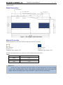
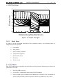
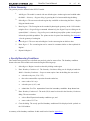
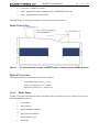
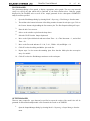
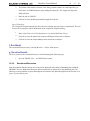
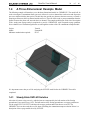
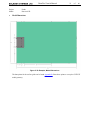
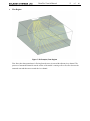
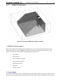
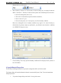
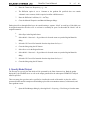
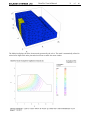
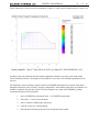
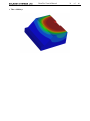
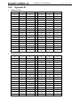
2D / 3D Contaminant Transport Modeling Software
Tutorial Manual
Written by:
Robert Thode, B.Sc.G.E.
Edited by:
Murray Fredlund, Ph.D.
SoilVision Systems Ltd.
Saskatoon, Saskatchewan, Canada
Software License
The software described in this manual is furnished under a license agreement. The software may be used or
copied only in accordance with the terms of the agreement.
Software Support
Support for the software is furnished under the terms of a support agreement.
Copyright
Information contained within this User’s Manual is copyrighted and all rights are reserved by SoilVision
Systems Ltd. The CHEMFLUX software is a proprietary product and trade secret of SoilVision Systems.
The User’s Manual may be reproduced or copied in whole or in part by the software licensee for use with
running the software. The User’s Manual may not be reproduced or copied in any form or by any means
for the purpose of selling the copies.
Disclaimer of Warranty
SoilVision Systems Ltd. reserves the right to make periodic modifications of this product without obligation
to notify any person of such revision. SoilVision does not guarantee, warrant, or make any representation
regarding the use of, or the results of, the programs in terms of correctness, accuracy, reliability, currentness,
or otherwise; the user is expected to make the final evaluation in the context of his (her) own problems.
Trademarks
Windows™ is a registered trademark of Microsoft Corporation.
SoilVision® is a registered trademark of SoilVision Systems Ltd.
SVOFFICE ™ is a trademark of SoilVision Systems Ltd.
SVFLUX ™ is a trademark of SoilVision Systems Ltd.
CHEMFLUX ™ is a trademark of SoilVision Systems Ltd.
SVAIRFLOW ™ is a trademark of SoilVision Systems Ltd.
SVHEAT ™ is a trademark of SoilVision Systems Ltd.
SVSOLID ™ is a trademark of SoilVision Systems Ltd.
SVDYNAMIC ™ is a trademark of SoilVision Systems Ltd.
ACUMESH ™ is a trademark of SoilVision Systems Ltd.
FlexPDE® is a registered trademark of PDE Solutions Inc.
Copyright © 2008
by
SoilVision Systems Ltd.
Saskatoon, Saskatchewan, Canada
ALL RIGHTS RESERVED
Printed in Canada
Table of Contents
...................................................................................................................................
1 ChemFlux Tutorial Manual
...................................................................................................................................
1.1 Introduction
...................................................................................................................................
1.2 Sudicky Model
1.2.1 Steady-State SVFLUX Model
...................................................................................................................................
1.2.2 CHEMFLUX Model
...................................................................................................................................
1.2.3 Appendix A
...................................................................................................................................
...................................................................................................................................
1.3 References
...................................................................................................................................
1.4 A Three-Dimensional Example Model
1.4.1 Steady-State SVFLUX Solution
...................................................................................................................................
1.4.2 Appendix B
...................................................................................................................................
3
of
40
4
6
6
6
13
22
23
24
24
39
ChemFlux Tutorial Manual
1
ChemFlux Tutorial Manual
2D / 3D Contaminant Transport Modeling
Software
Tutorial Manual
Written by:
Robert Thode, B.Sc.G.E.
Edited by:
Murray Fredlund, Ph.D.
SoilVision Systems Ltd.
Saskatoon, Saskatchewan, Canada
4
of
40
ChemFlux Tutorial Manual
5
of
40
Software License
The software described in this manual is furnished under a license agreement. The software may be used or
copied only in accordance with the terms of the agreement.
Software Support
Support for the software is furnished under the terms of a support agreement.
Copyright
Information contained within this Tutorial Manual is copyrighted and all rights are reserved by SoilVision
Systems Ltd. The CHEMFLUX software is a proprietary product and trade secret of SoilVision Systems.
The Tutorial Manual may be reproduced or copied in whole or in part by the software licensee for use with
running the software. The Tutorial Manual may not be reproduced or copied in any form or by any means for
the purpose of selling the copies.
Disclaimer of Warranty
SoilVision Systems Ltd. reserves the right to make periodic modifications of this product without obligation to
notify any person of such revision. SoilVision does not guarantee, warrant, or make any representation
regarding the use of, or the results of, the programs in terms of correctness, accuracy, reliability, currentness, or
otherwise; the user is expected to make the final evaluation in the context of his (her) own models.
Trademarks
WindowsÔ is a registered trademark of Microsoft Corporation.
SoilVisionÒ is a registered trademark of SoilVision Systems Ltd.
SVOFFICE Ô is a trademark of SoilVision Systems, Ltd.
CHEMFLUX Ô is a trademark of SoilVision Systems Ltd.
SVFLUX Ô is a trademark of SoilVision Systems Ltd.
SVHEAT Ô is a trademark of SoilVision Systems Ltd.
SVAIRFLOW Ô is a trademark of SoilVision Systems Ltd.
SVSOLID Ô is a trademark of SoilVision Systems Ltd.
SVDYNAMIC Ô is a trademark of SoilVision Systems Ltd.
ACUMESH Ô is a trademark of SoilVision Systems Ltd.
FlexPDEÒ is a registered trademark of PDE Solutions Inc.
Copyright Ó 2008
by
SoilVision Systems Ltd.
Saskatoon, Saskatchewan, Canada
ALL RIGHTS RESERVED
Printed in Canada
ChemFlux Tutorial Manual
1.1
6
of
40
Introduction
The Tutorial Manual serves a special role in guiding the first time users of the CHEMFLUX software through
a typical example problem. The example is "typical" in the sense that it is not too rigorous on one hand and
not too simple on the other hand.
The Tutorial Manual serves as a guide by: assisting the user with the input of data necessary to solve the
boundary value problem, ii.) explaining the relevance of the solution from an engineering standpoint, and iii.)
assisting with the visualization of the computer output. An attempt has been made to ascertain and respond to
questions most likely to be asked by first time users of CHEMFLUX.
1.2
Sudicky Model
Sudicky (1989) developed the following example. The model considers flow and solute transport in a
heterogeneous cross section with a highly irregular flow field, dispersion parameters that are small compared
with the spatial discretization, and a large contrast between longitudinal and transverse dispersivities (Zheng
and Wang, 1999).
It is important to note that you will be analyzing the SVFLUX model before the CHEMFLUX model is
completed.
1.2.1
Steady-State SVFLUX Model
The completed model is present under the project and model listed below. The user may open this model to
run and display the results of the analysis. The user can also recreate this model under a separate model file.
Project:
Model:
Minimum authorization required:
ContaminantPlumes
VanderHeijdeSS, VanderHeijde
FULL
The seepage model shown below gives the model dimensions, boundary conditions, material properties, and
the final flow regime. This is followed by step by step instructions on how to enter and solve the contaminant
ChemFlux Tutorial Manual
7
of
40
transport model.
Model Description
Figure 1 - 2D example, model dimensions
Material Properties
Material Properties used for the SVFLUX steady-state model are as follows:
k sat = 158 m/yr
k y-ratio = 1.0
Volumetric water content = 0.35
ksat = 3156 m/yr
k y-ratio = 1.0
Volumetric water content = 0.35
The soil-water characteristic curve data was used for both materials in the model.
Table 1
Soil Suction (kPa)
0.0001
100
1000
Volumetric Water Content Ratio
0.351
0.35
0.349
NOTE:
Steady-state seepage solutions do not require that the soil-water characteristic curves have an initial
positive slope. An initial positive slope is only required in transient models where water storage will
change with time. The initial positive slope on the SWCC applies for the low suction range.
8
ChemFlux Tutorial Manual
of
40
· SVFLUX Flow Regime
7
6
Elevation (m)
5
4
3
2
1
0
0
100
200
Distance Along Flow Direction (m)
Figure 2 - 2D example, flow regime
1.2.1.1
Model Setup
In order to set up the model described in the preceding section, the following steps (or
categories) will be required:
a.
Create model
b.
Enter geometry
c.
Specify boundary conditions
d.
Apply material properties
e.
Specify model output
f.
Run model
g.
Visualize results
a. Create Model
Since FULL authorization is required for this tutorial, the user must perform the following steps to ensure full
authorization is activated:
1.
Plug in the USB security key,
2.
Go to the File > Authorization dialog on the SVOFFICE Manager.
3.
Software should display full authorization of Standard or Professional. If not, it means that the
security codes provided by SoilVision Systems at the time of purchase have not yet been
ChemFlux Tutorial Manual
9
of
40
entered. Please see the the Authorization section of the SVOFFICE User's Manual for
instructions on entering these codes.
The following steps are required to create the model:
1.
Open the SVOFFICE Manager dialog.
2.
Select "ALL" under the Applications combo box and "ALL" for the Model Origin combo box.
3.
Create a new project called UserTutorial by pressing the New button next to the list of projects.
4.
Create a new model called User_Vanderheijde by pressing the New button next to the list of
models. The new model will be automatically added under the recently created UserTutorial
project. Use the settings below when creating a new model.
5.
Select the following:
·
SVFlux for Application
·
2D for System,
·
Steady-State for Type,
·
Metric for Units, and
·
Seconds (s) for Time Units.
Click on OK.
Before entering any model geometry it is best to set the World Coordinate System to ensure that the model
will fit into the drawing space.
1.
Access the World Coordinate System tab by selecting the World Coordinate System tab on the
Create New Model dialog.
2.
Enter the World Coordinates System coordinates shown below into the dialog.
x-minimum = -10
y-minimum = -2
x-maximum = 260
y-maximum = 8
3.
Click OK to close the dialog.
For better viewing results, set the magnification factor in the View Settings:
1.
Select View > Settings from the menu.
2.
Set the aspect ratio near 1:10. This will magnify the model's height.
3.
Click OK to close the dialog.
ChemFlux Tutorial Manual
10
of
40
b. Enter Geometry
The geometry must be defined for the SVFLUX model.
1.
Add Region: The model is created with one default region. Another region can be added under
the Model > Geometry > Regions dialog by pressing the New button and closing the dialog.
2.
Select Region: The user must select the region they would like to draw using the Draw > Region
Polygon from the menu.
3.
Draw Region 1: The first region can be extended by drawing the geometry on the CAD window
using the Draw > Region Polygon command. Alternatively, the Region Properties dialog can be
opened (Model > Geometry > Region Properties) and the region polyline points cut and pasted
in from the provided spreadsheet. The points can also be pasted into the dialog. See Appendix
A for the geometry of each region.
4.
Select Region 2: The user must select Region 2 as the current region on which to draw.
5.
Draw Region 2: The second region can be entered in a manner similar to that explained for
Region 1.
6.
Repeat for Region 3.
c. Specify Boundary Conditions
Flow models must generally have a defined entry and exit point for water to flow. The boundary conditions
shown at the start of this model can be entered using the following steps:
1.
Select Region 1: Region 1 must be selected by clicking on the region.
2.
Enter Boundary Conditions #1: The Boundary Conditions dialog can be displayed under the
Model > Boundary Conditions > Properties menu option. Once in the dialog the user needs to:
3.
·
select the node point, (250, 5.375),
·
then select a normal flux expression from the combo box,
·
enter a value of 0.1 m/yr.
·
select the point (0, 6.5), and
·
select the Zero Flux expression from the boundary condition drop-down box.
Enter Boundary Condition #2: The node (250,0) must be selected in the Boundary Conditions
dialog. The user must then:
4.
·
select a Head Expression boundary condition type, and
·
enter a value of 5.375 m.
Close the dialog. The newly specified boundary condition will be displayed with symbols on
the CAD window.
A summary of the boundary conditions for this model can be found in Appendix A.
ChemFlux Tutorial Manual
11
of
40
d. Apply Material Properties
Material Properties must now be entered and applied to specific regions in the model. The following steps are
required in order to properly apply material properties:
1.
Open Materials Manager: Model > Material > Manager.
2.
Click New: This will open a new material record. Enter ChemFlux Soil1 as the material name and
click OK.
3.
Enter Properties: The material properties for ChemFlux Soil1 must be entered. Click the
Properties button on the Material Manager dialog.
4.
Laboratory SWCC data: Choose the SWCC tab and click the Data button. Enter the material
properties as found in Table 1. Click OK to accept the data entered and close the SWCC Data
dialog.
5.
Fitting: Laboratory data can be best fit with the Fredlund & Xing (1994) soil-water
characteristic curve equation. Fitting the curve can be accomplished through the following steps:
6.
a.
Select Fredlund & Xing as the fitting method from the SWCC drop-down.
b.
Enter 0.351 in the field for Saturated VWC.
c.
Click the Properties button to set the properties of the Fredlund & Xing fit.
d.
Click the Apply Fit button.
Enter the Hydraulic Conductivity data: Choose the Hydraulic Conductivity Tab and enter the K
sat
and Ky-ratio values. The dialog can be closed once material properties are entered. The
ChemFlux Soil2 material's properties are available in Appendix A and can be entered in the
same manner as ChemFlux Soil1.
7.
Apply to regions: The material properties can be applied to regions by opening the Regions
dialog (Model > Geometry > Regions) and selecting the appropriate materials from the dropdown boxes. ChemFlux Soil1 should be applied to Region 1 and ChemFlux Soil2 should be
applied to Regions 2 and 3.
e. Specify Model Output
Two levels of output may be specified: i) output (graphs, contour plots, fluxes, etc.) which are displayed
during model solution, and ii) output which is written to a standard finite element file for viewing with
AcuMesh software. Output is specified in the following two dialogs in the software:
i) Plot Manager:
ii) Output Manager:
Output displayed during model solution.
Standard finite element files written out for visualization in AcuMesh or for
initial condition input to other finite element packages.
12
ChemFlux Tutorial Manual
of
40
PLOT MANAGER
The plot manager dialog is first opened to display appropriate solver graphs. There are many plot types
that can be specified to visualize the results of the model. A few will be generated for this tutorial example
model, including a plot of the solution mesh, pressure contours, head contours, and gradient vectors.
1.
Open the Plot Manager dialog by selecting Model > Reporting > Plot Manager from the menu.
2.
The toolbar at the bottom left of the dialog contains a button for each plot type. Click on the
Contour button to begin adding the first contour plot. The Plot Properties dialog will open.
3.
Enter the title 'Pressure'.
4.
Select 'u' as the variable to plot from the drop-down.
5.
Click the Output Options tab and ensure that only Plot is checked off.
6.
Click OK to close the dialog and add the plot to the list.
7.
Repeat steps 2 to 6 to create the plots shown in the above dialog. The zoomed plots are not
necessary, they are used to closely examine key zones in the problem.
8.
Click OK to close the Plot Manager and return to the workspace.
Alternatively, the user may press the Add Default Plots button and typical plots will be added to the plot
list.
OUTPUT FILES
There are four output file types that can be specified to export the results of the model. One will be
generated for this tutorial example model: a plot to transfer the results to ACUMESH.
1.
Open the Output Manager dialog by selecting Model > Reporting > Output Manager from the
menu.
2.
The toolbar at the bottom left corner of the dialog contains a button for each output file type.
Click on the ACUMESH button to add the output file with the default variables.
3.
Press the CHEMFLUX button to add the output file with the default variables.
13
ChemFlux Tutorial Manual
of
4.
Click OK to close the dialog and add the output file to the list.
5.
Click the Settings button on the Output Manager dialog to open the Output Settings dialog.
6.
Ensure the Region Separation checkbox is checked; press OK to close the dialog.
7.
Click OK to close the Output Manager and return to the workspace.
40
f. Run Model
The current model can be run by selecting the Solve > Analyze menu option.
g. Visualize Results
The flow vectors for the current model can be visualized through the following steps:
1.2.1.2
1.
Open ACUMESH: View > ACUMESH menu option
2.
Plot Flow Lines: Plot > Flow Lines
Results and Discussion
7
Elevation (m)
6
5
4
3
2
1
0
0
100
200
Distance Along Flow Direction (m)
Figure 3 ACUMESH flowlines for steady-state flow regime.
1.2.2
CHEMFLUX Model
Now that the steady-state flow hydraulic head gradients have been established in the SVFLUX software the
focus turns to solving for the chemical concentrations with time for the solution domain. In order to solve this
model the user needs to perform the following steps:
ChemFlux Tutorial Manual
1.
Create a new CHEMFLUX model,
2.
Apply appropriate boundary conditions in the CHEMFLUX model, and
3.
Apply appropriate material properties.
14
of
40
The methodology for setting up the model is detailed in the following sections.
Model Description
Figure 4 - The 2D Vanderheijde example, showing boundary conditions for the CHEMFLUX model
Material Properties
The material properties for the numerical model are as follows:
Longitudinal Dispersivity, aL = 0.5m
Transverse Dispersivity, aT = 0.005m
Diffusion Coefficient, D* = 0.0423m2/yr
1.2.2.1
Model Setup
In order to set up the model described in the preceding section, the following steps are required. The steps fall
under the general categories of:
a.
Create model
b.
Enter geometry
c.
Specify boundary conditions
d.
Apply material properties
e.
Specify model output
f.
Run model
ChemFlux Tutorial Manual
g.
15
of
40
Visualize results
a. Create Model
A gradient file generated by SVFLUX is required for this example. The seepage model described above has
been included in the model files distributed with the SVFLUX software. This file was generated previously in
the Steady-State SVFLUX model example.
When the solution for the model is finished, a gradient file will be automatically created in the solution folder
by SVFLUX. The file is called gradient.trn.
The user must decide the project under which the CHEMFLUX model is going to be organized. If the project
is not yet included in the Projects section of the SVOFFICE Manager, you must add the project before
proceeding with creating the model. In this case, the model is placed under the project called UserTutorial. To
add a model:
1.
Open the SVOFFICE Manager dialog.
2.
Select the project called UserTutorial.
3.
Press the New button under the Models heading.
4.
Select CHEMFLUX for the Application.
5.
Enter User_Example2D in the Model Name box.
6.
Select 2D for System, Transient for Type, Metric for Units, and Years for Time Units.
7.
Click the OK button to save the model and close the New Model dialog.
8.
The new model will automatically added be added to the Models list.
NOTE:
You will notice that there is no distinction between steady-state and transient state in
CHEMFLUX. This is because all CHEMFLUX models are considered to be transient state.
b. Enter Geometry
The geometry for the model can be obtained in the spreadsheet located here. Entering the geometry into the
newly created SVFLUX model can be accomplished through the following steps:
1.
Select the Model > Geometry > Import Geometry > From Existing Model... menu.
2.
The Import Geometries dialog will pop up. Select the appropriate project name, Tutorial.
3.
Select the Vanderhiejde model.
4.
Press the Import button.
The World Coordinate Settings and the View Settings may need to be set up again:
1.
Access the World Coordinate System dialog by selecting View > World Coordinate System from
ChemFlux Tutorial Manual
16
of
40
the menu.
2.
Enter the World Coordinates System coordinates shown below into the dialog.
x-minimum = -10
y-minimum = -2
x-maximum = 260
y-maximum = 8
3.
Click OK to close the dialog.
For better viewing results, set the magnification factor in the View Settings:
1.
Select View > Settings from the menu.
2.
Set the aspect ratio near 1:10. This will magnify the model's height.
3.
Click OK to close the dialog.
c. Specify Boundary Conditions
In general, flow models must have a defined entry and exit point for water to flow. The boundary conditions
shown at the start of this model may be entered through the following steps:
1.
Select Region 1: Region 1 must be selected by clicking on the region.
2.
Enter Boundary Conditions: The Boundary Conditions dialog may be displayed under the Model
> Boundary Conditions > Properties menu option. Once in the dialog the user needs to:
·
Select the point (0,0) from the list,
ChemFlux Tutorial Manual
·
17
of
40
From the Boundary Condition drop-down select a Flux Expression boundary condition
equal to 0,
·
Repeat these steps to define the boundary conditions for the remaining Region 1 segment
as shown in the diagram and in the screen-shot above. (Be sure to define a Flux Expression
boundary condition equal to 0 for the last point in the list).
3.
Close the dialog. The newly specified boundary condition will be displayed with symbols on
the CAD window.
d. Apply Material Properties
Material Properties must now be entered and applied to specific regions in the model. The following steps are
required in order to properly apply material properties:
1.
Open Materials Manager: Model > Material > Manager.
2.
Click New: This will open a new material record.
3.
Enter Properties: Move to the Dispersion tab. Enter the Longitudinal Dispersivity, aL = 0.5 m.
Enter the Transverse Dispersivity, aT = 0.005 m. Select Constant as the Diffusion option.
Enter the Diffusion Coefficient, D* = 0.0423 m2/yr.
4.
Apply to regions:
·
Open the regions dialog selecting Model > Geometry > Regions from the menu.
·
Select Material#1 from the drop-down as the material for Region 1.
·
Repeat for Region 2 and Region 3.
·
Click OK to close the dialog.
Next, the settings that will be used for the model must be specified. To open the Settings dialog select Model >
Settings in the workspace menu.
The Settings dialog will contain information about the current model System, Units, Time, and contaminant
transport processes.
1.
To open the Settings dialog select Model > Settings in the workspace menu.
2.
Check Advection and Dispersion in the Processes box under the General tab.
3.
Choose the Time tab. Enter a Start Time of 0, a Time Increment of 1 yr, and an End Time of 20
yr.
4.
Select the Advection tab.
5.
Choose Import from the Advection Control option.
6.
Click Browse.
7.
Specify the gradient file Examples_ChemFlux2D.trn that was generated by SVFLUX in the
ChemFlux Tutorial Manual
18
of
40
previous example.
8.
Press OK to close the Settings dialog.
NOTE:
It is very important that the .TRN file and the geometry are obtained from the same SVFLUX
model.
e. Specify Model Output
Two levels of output may be specified: i) output (graphs, contour plots, fluxes, etc.) which are displayed
during model solution, and ii) output which is written to a standard finite element file for viewing with
AcuMesh software. Output is specified in the following two dialogs in the software:
i) Plot Manager:
ii) Output Manager:
Output displayed during model solution.
Standard finite element files written out for visualization in AcuMesh or for
inputting to other finite element packages.
ChemFlux Tutorial Manual
19
of
40
PLOT MANAGER
The plot manager dialog is first opened to display appropriate solver graphs. The next step in model
setup is to specify the data which will be generated by the finite element solver. Both the graphs
displayed by the FlexPDE solver as well as the output generated for the subsequent CHEMFLUX
analyses must be specified.
1.
Open the Plot Manager dialog by selecting Model > Reporting > Plot Manager from the menu.
2.
The toolbar at the bottom left corner of the dialog contains a button for each plot type. Click on
the Contour button to begin adding the first contour plot. The Plot Properties dialog will open.
3.
Enter the title Concentration.
4.
Select c as the variable to plot from the drop-down.
5.
Select the PLOT from the Output Option tab.
6.
Move to the Update Method tab and enter a Start Time = 0, a Time Increment = 1, and an End
Time = 20.
7.
Move to the Zoom tab and enter X = 100, Y = 0.1, Width = 100, and Height = 6.6.
8.
Click OK to close the dialog and add the plot to the list.
9.
Repeat steps 2 to 8 to create the remaining plots. Note that the Mesh plot does not require
entry of a variable.
10. Click OK to close the Plot Manager and return to the workspace.
OUTPUTMANAGER
There are many output file types that can be specified to export the results of the model. One will be
generated for this tutorial example model: a file to transfer the results to ACUMESH.
1.
Open the Output Manager dialog by selecting Model > Reporting > Output Manager from the
menu.
ChemFlux Tutorial Manual
2.
20
of
40
The toolbar at the bottom left corner of the dialog contains a button for each output file type.
Click on the ACUMESH button to begin adding the output file. The Output File Properties
dialog will open.
3.
Enter the title ACUMESH.
4.
Click OK to close the dialog and add the output file to the list.
Specify Time Steps:
The Output File Properties dialog also allows the user to define timesteps for the current model. This can
be accessed by using the Update Method tab on the Output File Properties dialog.
1.
Enter a Start Time of 0, a Time Increment of 1 yr, and an End Time of 20 yr.
2.
Click OK to close the Output File Properties dialog and return to the workspace.
3.
Click OK to close the Output Manager and return to the workspace.
f. Run Model
The current model may be run by selecting the Solve > Analyze menu option.
g. Visualize Results
The flow vectors for the current model may be visualized through the following steps:
1.
1.2.2.2
Open ACUMESH: View > ACUMESH menu option.
Results and Discussion
After the model has finished solving, the results will be displayed in the dialog of thumbnail plots within the
CHEMFLUX solver. Right-click the mouse and select Maximize to enlarge any of the thumbnail plots. The
following is a short summary of plots illustrating the movement of the plume through the model for times of 8
years, 12 years, and 20 years.
ChemFlux Tutorial Manual
·
Time = 8 years
The source has been shut off for 3 years
·
Time = 12 years
21
of
40
22
ChemFlux Tutorial Manual
·
Time = 20 years
1.2.3
Appendix A
Region 1
X
0
250
250
175
125
80
40
0
Region 2
Y
0
0
5.375
5.5
6.333
6.393
6.447
6.5
X
0
120
120
0
Region 3
Y
2
2
4
4
X
180
250
250
180
Y
2
2
4
4
of
40
ChemFlux Tutorial Manual
23
of
40
Boundary Conditions
X
0
250
Y
0
0
Boundary Condition
Gradient Expresion = 0
Continue
250
175
125
80
40
0
5.375
5.5
6.333
6.393
6.447
6.5
Concentration Expression = 0
Continue
Continue
Concentration Expression = if t <= 5 then 1 else 0.
Concentration Expression = 0
Gradient Expresion = 0
1.3
References
C.W. Fetter, 1994. Applied Hydrogeology, Third Edition. Prentice-Hall, Inc. Upper Saddle
River, New Jersey.
C.W. Fetter, 1993. Contaminant Hydrogeology. MacMillan Publishing Company. New York,
New York.
D. G. Fredlund and H. Rahardjo, 1993. Soil Mechanics for Unsaturated Soils. John Wiley &
Sons, New York
FlexPDE 3.x Reference Manual, 1999. PDE Solutions Inc. Antioch, CA 94509
Jacob Bear, 1972. Dynamics of Fluids in Porous Media. Dover Publications Inc., New York
Jacob Bear, 1979. Hydraulics of Groundwater. McGraw-Hill, New York.
Jason S. Pentland, 2000. Use of a General Partial Differential Equation Solver for Solution of
Heat and Mass Transfer Problems in Soils. University of Saskatchewan, Canada
Nguyen Thi Minh Thieu, 1999. Solution of Saturated/Unsaturated Seepage Problems Using a
General Partial Differential Equation Solver. University of Saskatchewan, Canada
R. Allan Freeze and John A. Cherry, 1979. Groundwater. Prentice –Hall, Inc., Englewood
Cliffs, New Jersey
Tecplot User’s Manual, version 8.0, 1999. Amtec Engineering Inc. Bellevue, WA 98009-3633
ChemFlux Tutorial Manual
1.4
24
of
40
A Three-Dimensional Example Model
The following example will introduce you to the three-dimensional model in CHEMFLUX. The model will be
used to investigate if contaminant from a reservoir will travel to a river channel due to advection and dispersion
processes within a 400 day time period. The 400 day time period was chosen as the time necessary to install a
pumping well between the river channel and the reservoir. The well will be used to pump contaminant from the
ground to ensure the plume will not reach the river channel. The example model begins with a brief description
of the steady-state seepage analysis completed to provide CHEMFLUX with computed seepage gradients.
Next a detailed set of instructions guides the user through the creation of the 3D contaminant transport model.
Project:
Model:
Minimum authorization required:
Tutorial
Example3D
FULL
It is important to note that you will be analyzing the SVFLUX model before the CHEMFLUX model is
completed.
1.4.1
Steady-State SVFLUX Solution
Advection is known as the process by which solutes are transported by the bulk motion of the flowing
groundwater Freeze and Cherry (1979). The bulk motion of the flowing groundwater or seepage gradients are
solved using SVFLUX. SVFLUX calculates the seepage gradients and writes them to a text file. The
CHEMFLUX solver then reads this text file when calculating the contaminant transport solution. Below is a
description of the seepage model solved by SVFLUX.
ChemFlux Tutorial Manual
Project:
Model:
·
25
of
40
Ponds
Reservoir3D
Model Dimensions
Figure 5 3D Example; Model Dimensions
The data points for the surface grids can be found Appendix B. Enter these points to set up the SVFLUX
model geometry.
ChemFlux Tutorial Manual
·
26
of
40
Boundary Conditions
Figure 6 3D Example; Boundary Conditions
The steady-state seepage model is set up to simulate a pond or reservoir a certain distance from a river
channel. The water levels in the reservoir and river channel are set using head boundary conditions. The
level of water in the reservoir is set using a Head Expression = 10.5m set on surface 2 for the reservoir
region. The level of water in the river channel is set using a Head Expression = 7m set on the line segment
extending from point (14,0) to (14,27) on surface 1.
·
Material Properties
There is only one material in the saturated 3D example model. Two regions have been implemented in this
model in order to apply the necessary boundary conditions. The material in the model has a hydraulic
conductivity, k sat = 2.17e –01 m/d.
ChemFlux Tutorial Manual
·
27
of
40
Flow Regime
Figure 7 3D Example; Flow Regime
Flow lines show that groundwater is flowing from the reservoir toward the adjacent river channel. The
presence of unsaturated material near the surface of the model is causing water to first flow down to the
saturated zone and then move toward the river channel.
ChemFlux Tutorial Manual
1.4.1.1
28
of
40
CHEMFLUX Model Setup
Figure 8 3D example, CHEMFLUX boundary conditions
· CHEMFLUX Material Properties
Please note the SVFLUX Solution shown in the diagrams above are a result of the SVFLUX Reservoir3D
Tutorial. In order to set up the CHEMFLUX model described for this tutorial, the following steps will be
required. The steps for creating a model fall under the general categories of:
1.
Create model
2.
Enter geometry
3.
Specify boundary conditions
4.
Apply material properties
5.
Specify model output
6.
Run model
7.
Visualize results
1. Create Model
The first step in defining a model is to decide the project under which the model is going to be organized. If the
project is not yet included you must add the project before proceeding with the model. In this case, the model
ChemFlux Tutorial Manual
29
of
40
is placed under the project called Tutorial. To add a model:
1.
Open the SVOFFICE Manager dialog.
2.
Select the project called UserTutorial.
3.
Press the New button under the Models heading and enter User_CHEMFLUX3D as the model
title.
4.
Select the following:
·
CHEMFLUX for Application
·
3D for System,
·
Transient for Type,
·
Metric for Units, and
·
Days for Time Units.
5.
Click the OK button to save the model and close the New Model dialog.
6.
The new model will automatically be opened in the workspace.
2. Enter Geometry
The geometry for the model must be imported from SVFLUX before any other modeling can be done in
CHEMFLUX.
1.
Select the Model > Geometry > Import Geometry > From Existing Model... menu.
2.
The Import Geometries menu will pop up. Select the appropriate project name Tutorials.
3.
Select the Reservoir3D model.
4.
Press the Import button.
5.
A Pop up message will appear stating Current surfaces, geometry, features, art objects, flux
sections, and plots referencing a specific region to be deleted. Do you wish to continue? Click
on Yes.
6.
A Pop up message will appear asking if you want to copy material properties and assignments.
Click on No.
The import includes any regions, region shapes, surfaces, surface grids and elevations. These parts of the
model definition are fixed in CHEMFLUX. World coordinate system settings and features are also imported if
present, but may be edited in CHEMFLUX.
3. Specify Boundary Conditions
In general, flow models must have a defined entry and exit point for water to flow. The boundary conditions
shown at the start of this model may be entered through the following steps:
1.
Select Region 1: Slope and Surface: 1 must be selected by clicking on the region & surface
ChemFlux Tutorial Manual
30
of
40
dialogue at the top of the screen.
2.
Enter Boundary Conditions #1: The Boundary Conditions dialog may be displayed under the
Model > Boundaries > Boundary Conditions menu option. Once in the dialog the user needs to:
· Select the starting node point, (14, 0),
· Then select a Concentration expression from the combo box,
· Enter a value of 0.1 g/m3.
· Select the node point, (14, 27) and specify a zero flux boundary condition.
Please note, although the above boundary conditions may appear to be entered already by
default (from the geometry import you performed) , you still need to enter the above conditions
for CHEMFLUX analysis to occur.
3.
Close the dialog. The newly specified boundary condition will be displayed with symbols on
the CAD window.
4. Apply Material Properties
The next step in defining the model is to specify the settings that will be used for the model.
The Settings dialog will contain information about the current model System, Units, Time, and contaminant
transport processes.
1.
To open the Settings dialog select Model > Settings in the menu.
ChemFlux Tutorial Manual
2.
31
of
40
Put a check mark in the Advection and Dispersion boxes in the Processes section under the
General tab if they are not already there.
3.
Move to the Time tab.
4.
Enter a Start Time of 0, an Initial Increment of 50 days, and an End Time of 400 days.
5.
Select the Advection tab.
6.
Choose Import from the Advection Control option.
7.
Click Browse.
8.
Specify the file ChemfluxInput_Reservoir3D_1.trn that was generated by SVFLUX. This file
can be found in the following directory C:\SVS\ModelFilesSVSlope\Tutorial\3d\SteadyState
\Reservoir3D.
NOTE:
It is very important that the .TRN file and the geometry are obtained from the same SVFLUX
model.
In order to improve solution time for the purposes of this tutorial certain finite-element options will be set.
The finite element mesh node limit and grid spacing will be set to generate a simpler mesh that will reduce the
solution time.
9.
Select Model > FEM Options from the menu to open the FEM Options dialog.
10. Click on the Advanced>> button.
11. Click on the Mesh Generation Controls tab.
12. Set the NODELIMIT to 10000.
13. Press OK to close the FEM Options dialog.
The next step in defining the model is to enter the material properties for the single material that will be used in
the model. Only one material is used for the model with these properties:
Longitudinal Dispersivity, aL = 1m
Transverse Dispersivity, aT = 1m
Diffusion Coefficient, D* = 0m2/day
1.
Open the Materials Manager dialog by selecting Model > Materials > Manager… from the
menu.
2.
Click the New Material button to create a material, type in a name for the material as 3D
Tutorial Soil and click OK. The Material Properties dialog will open automatically.
3.
Move to the Dispersion tab.
4.
Refer to the data provided above. Enter the Longitudinal Dispersivity, aL = 1m.
ChemFlux Tutorial Manual
32
of
40
5.
Enter the Transverse Dispersivity, aT = 1m.
6.
The Diffusion option is set to Constant as the gradient file specified does not contain
volumetric water content, which is required to define a diffusion curve.
7.
Enter the Diffusion Coefficient, D* = 0m2/day.
8.
Close the Material Properties and Material Manager dialogs.
Each region will cut through all the layers in a model creating a separate “block” on each layer. Each block can
be assigned a material or be left as void. A void area is essentially air space. In this model all “blocks” will be
assigned a material.
1.
Select Slope in the Region Selector.
2.
Select Model > Materials > Region Materials from the menu to open the Region Materials
dialog.
3.
Select the 3D Tutorial Soil material from the drop-down for Layer 1.
4.
Close the dialog using the OK button.
5.
Select Reservoir in the Region Selector.
6.
Select Model > Materials > Region Materials from the menu to open the Region Materials
dialog.
7.
Select the 3D Tutorial Soil material from the drop-down for Layer 1.
8.
Close the dialog using the OK button.
5. Specify Model Output
The next step is to specify the data which will be generated by the finite element solver. Both the graphs
displayed by the FlexPDE solver as well as the output generated for the subsequent CHEMFLUX analysis
must be specified.
There are many plot types that can be specified to visualize the results of the model. A plots few will be
generated for this tutorial example model including a plot of the concentration contours, solution mesh, and
water gradient vectors.
1.
Open the Plot Manager dialog by selecting Model > Reporting > Plot Manager from the menu.
ChemFlux Tutorial Manual
2.
33
of
40
The toolbar at the bottom left corner of the dialog contains a button for each plot type. Click on
the Contour button to begin adding the first contour plot. The Plot Properties dialog will open.
3.
Enter the title Concentration.
4.
Select c as the variable to plot from the drop-down.
5.
Move to the Update Method tab.
6.
If not already entered, enter in the following values for Start = 0 Increment = 50 End = 400.
7.
Move to the Projection tab.
8.
Select Plane Projection option.
9.
Select Y from the Coordinate Direction drop-down.
10. Enter 14 in the Coordinate field. This will generate a 2D slice at Y = 14m on which the
concentration contours will be plotted.
11. Move to the Output Options tab.
12. Select the PLOT output option.
13. Click OK to close the dialog and add the plot to the list.
14. Repeat these steps 2 to 12 to create the plots shown above. Note that the Mesh plot does not
require entry of a variable under the Description Tab. Also note that the Solution Mesh &
Mesh should only have an entry value for Start under the Update Method tab, Time Steps.
15. Click OK to close the Plot Manager and return to the workspace.
There are a few output file types that can be specified to export the results of the model. One will be generated
for this tutorial example model: a file to output the results to AcuMesh for advanced visualization.
1.
Open the Output Manager dialog by selecting Model > Reporting > Plot Manager from the
menu.
ChemFlux Tutorial Manual
2.
34
of
40
The toolbar at the bottom left corner of the dialog contains a button for each output file type.
Click on the ACUMESH button to begin adding the output file. The Output File Properties
dialog will open.
3.
The title will be entered automatically as User_Example3D_AcuMesh.
4.
The variables c, vx, vy, and vz appear automatically as the default.
5.
Type in the following values under the Update Method, Time Steps. Start = 0 Increment = 40
End = 400.
6.
Click OK to close the dialog and add the output file to the list.
7.
Click OK to close the Output Manager and return to the workspace.
6. Run Model
The current model may be run by selecting the Solve > Analyze menu option.
7. Visualize Results
The flow vectors for the current model may be visualized through the following steps:
1.4.1.2
1.
Open ACUMESH: View > ACUMESH menu option
2.
Plot Contours: Plot > Contours
3.
Model State: States toolbar drop-down
Results and Discussion
After the model has finished solving, the results will be displayed in the dialog of thumbnail plots within the
CHEMFLUX solver. Right-click the mouse and select Maximize to enlarge any of the thumbnail plots. This
section will give a brief analysis for each plot that was generated.
ChemFlux Tutorial Manual
35
of
40
The Mesh plot displays the finite element mesh generated by the solver. The mesh is automatically refined in
critical areas. Right-click on the plot and select Rotate to enable the rotate window.
ChemFlux Tutorial Manual
36
of
40
In this contour plot it can be seen the concentration is equal to 1 at the reservoir and decreases to 0 at the river.
Gradient Vectors show both the direction and the magnitude of the flow at specific points in the model.
Vectors illustrate that flow is from right to left towards the river in this view with higher gradients near the
reservoir.
The following is a short summary of plots created in ACUMESH illustrating the movement of the plume
through the model for times of 50 days, 100 days, and 400 days. Note that the plume does not reach the river
channel in within the 400 day time period. The below diagram was created in ACUMESH by plotting
concentration contours and varying time:
1.
Open ACUMESH by selecting Window > ACUMESH from the menu.
2.
Select Plots > Contours from the menu.
3.
Select c from the Variable Name drop-down.
4.
Click OK to close the Contours dialog.
5.
Select the desired timestep from the Time drop-down on the toolbar.
ChemFlux Tutorial Manual
· Time = 50 days
· Time = 100 days
37
of
40
ChemFlux Tutorial Manual
· Time = 400 days
38
of
40
39
ChemFlux Tutorial Manual
1.4.2
·
Appendix B
Surface 1 Grid
X
0
0
0
0
0
0
2
2
2
2
2
2
3
3
3
3
3
3
·
Y
0
10
11
16
17
27
0
10
11
16
17
27
0
10
11
16
17
27
Z
0
0
0
0
0
0
0
0
0
0
0
0
0
0
0
0
0
0
X
14
14
14
14
14
14
21
21
21
21
21
21
24
24
24
24
24
24
Y
0
10
11
16
17
27
0
10
11
16
17
27
0
10
11
16
17
27
Z
0
0
0
0
0
0
0
0
0
0
0
0
0
0
0
0
0
0
Y
0
10
11
16
17
27
0
10
11
16
17
27
0
10
11
16
17
27
Z
11
11
10
10
11
11
11
11
10
10
11
11
11
11
11
11
11
11
X
14
14
14
14
14
14
21
21
21
21
21
21
24
24
24
24
24
24
Y
0
10
11
16
17
27
0
10
11
16
17
27
0
10
11
16
17
27
Z
11
11
11
11
11
11
4
4
4
4
4
4
4
4
4
4
4
4
Surface 2 Grid
X
0
0
0
0
0
0
2
2
2
2
2
2
3
3
3
3
3
3
of
40


![RUMD User Manual [Version 3.0]](http://vs1.manualzilla.com/store/data/005734566_1-539a984f38202face31c4a646ef91457-150x150.png)