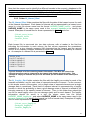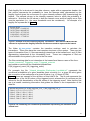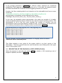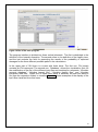
1
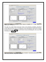
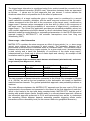
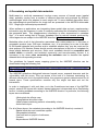
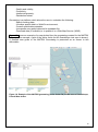
Project number: Project name: Project acronym: Theme: Start date: 265138 New methodologies for multi-hazard and multi-risk assessment methods for Europe MATRIX ENV.2010.6.1.3.4 Multi-risk evaluation and mitigation strategies 01.10.2010 End date: 31.12.2013 (39 months) Deliverable: D3.5: Software for multi-hazard assessment Version: Final Responsible partner: AMRA Month due: M38 Month delivered: M40 Primary authors: Alexander Garcia-Aristizabal Warner Marzocchi _______________________________ Signature 12.2013 _________________ Date Reviewer: Kevin Fleming _______________________________ Signature 12.2013 _________________ Date Authorised: Kevin Fleming _______________________________ Signature 01.2014 _________________ Date Dissemination Level PU Public Restricted to other programme participants (including the Commission PP Services) Restricted to a group specified by the consortium (including the RE Commission Services) CO Confidential, only for members of the consortium (including the Commission Services) RE 1 2 Abstract The multi-hazard concept can be seen as the process of assessing both different (independent) hazards threatening a given (common) area, and the possible interactions or cascade effects among the different hazardous events. In the MATRIX deliverable D3.4, a formal probabilistic framework to describe the multi-hazard problem from the perspective of cascading effects was presented. This report accompanies a simple software tool in which the theoretical framework described in D3.4 has been implemented in order to test the effects of considering different interaction levels when assessing cascading effects in a multi-hazard analysis. This software is a very simple tool whose potential use is mainly for academic and demonstrative applications, but with little effort could be extended to perform more detailed analyses and risk calculations. The idea to keep it simple, with it only calculating damage probabilities (for single damage states) is to highlight the effects of the possible interactions on the final calculation of risk. Disclaimer: This software is a demonstrative tool based on the conceptual framework defined in the WP3 of the MATRIX project. It is mainly intended for academic use, and the authors accept no liability for the content of the code, or for the consequences of any actions taken on the basis of the information provided. Keywords: Multi-hazard assessment, Cascading effects, Interactions, Software 3 4 Acknowledgments The research leading to these results has received funding from the European Commission’s Seventh Framework Programme [FP7/2007-2013] under grant agreement n° 265138. Different partners from the MATRIX project have collaborated in the preparation of this report. Here we include the entire list of people who participated (alphabetical order of institutions): - AMRA: Alexander Garcia-Aristizabal, Warner Marzocchi - BRGM: Daniel Monfort Climent, Etienne Taffoureau 5 6 Table of contents 1 Introduction ............................................................................................................................................. 10 2 Multi-hazard assessment for cascading effects: considering interactions.............................................. 11 2.1 Interactions at the hazard level .......................................................................................................... 11 2.2 Interactions at the vulnerability level................................................................................................. 13 3 Description of the implemented software tool ....................................................................................... 15 3.1 ABOUT THE Development environment ............................................................................................ 15 3.2 Required files and installation ............................................................................................................ 15 3.2.1 Main program script: AssessInteractionsX.0.py ...................................................................... 16 3.2.2 Folder 01_scenario_database/ ................................................................................................ 17 3.2.3 Folder 02_Hazard_files/ .......................................................................................................... 18 3.2.4 Folder 03_Fragility_files/ ......................................................................................................... 18 3.2.5 Folder 04_interactions/ ........................................................................................................... 19 3.2.6 Folder help_mhaz/ .................................................................................................................. 20 3.3 Description of the Graphical user interface (GUI) .............................................................................. 20 3.3.1 The Hazard term ...................................................................................................................... 22 3.3.2 The fragility term ..................................................................................................................... 24 3.3.3 The expected damage estimation panel ................................................................................. 25 3.4 Description of event interactions within the matrix-city tool ............................................................ 27 4 Geocatalog and spatial data metadata ................................................................................................... 29 5 Final Remarks .......................................................................................................................................... 31 6 References ............................................................................................................................................... 32 7 List of Figures Figure 1 Probability surface represented by p(IM1i,j), for i>1, j>1, as presented in Equation 1. ........................................................................................................................................ 13 Figure 2 Fragility surface for the case of seismic and volcanic ash loading acting simultaneously on the roofs in Naples, Italy (derived from the data in Zuccaro et al., 2008). ........................................................................................................................................... 14 Figure 3 Structure of files and folders of the system .......................................................... 16 Figure 4 Format of the data contained in the file “scenario_database.txt”. ....................... 17 Figure 5 Example of cascading scenarios ......................................................................... 17 Figure 6 Example of a file containing hazard information. The IM is the value of the intensity measure used to characterize the hazard (with known physical units). This example is simply to illustrate the process we follow (as will be done in the subsequent figures). .............................................................................................................................. 18 Figure 7 Example of a file containing fragility information. Note that the IM thresholds selected to represent the fragility function are the same used to represent the hazard. .... 19 Figure 8 File containing the conditional probabilities representing an interation at the hazard level ....................................................................................................................... 19 Figure 9 Example of a file containing information of a fragility surface to assess interactions at the vulnerability level .................................................................................. 20 Figure 10 GUI of the main program. .................................................................................. 21 Figure 11 Examples of file visualization functions from the menu "Database". .................. 22 Figure 12 Example of the plot hazard surface function for two interacting hazards. .......... 23 Figure 13 Example of the hazard interaction calculation.................................................... 23 Figure 14 Example of the plot of the fragility surface arising from considering interactions at the vulnerability level...................................................................................................... 24 Figure 15 Example of calculation of the damage probability for a single hazard (no interactions, see Table 2)................................................................................................... 26 Figure 16 Example of the damage probability calculation considering interactions at the vulnerability level with independent hazards. ..................................................................... 26 Figure 17 Example of the damage probability calculation considering interactions at both the hazard and the vulnerability levels. .............................................................................. 27 Figure 18: Example of the MATRIX geocatalog (active faults file) for the case of Guadeloupe, French West Indies. ..................................................................................... 30 8 List of Tables Table 1 Description of the structure of files necessary to run the system for the assessment of interactions ................................................................................................ 16 Table 2 Possible combinations to calculate the damage probability. ................................. 25 Table 3 Example of the correlation matrix between wind hazard (wind and track) and storm surge hazard (from Mignan et al., 2013b). ............................................................... 28 9 1 Introduction Multi-hazard is a wide concept that we can divide into two possible lines of applications: (1) multi-hazard assessment seen as the process to assess different (independent) hazards threatening a given (common) area, and (2) multi-hazard assessment seen as the process to assess possible interactions or cascade effects among the different hazardous events. In the MATRIX deliverable D3.4 (Garcia-Aristizabal et al., 2013), a formal probabilistic framework to describe the multi-hazard problem from the perspective of cascading effects was presented. This report accompanies a simple software tool in which the theoretical framework described in D3.4 has been implemented in order to test the effects of considering different interaction levels when assessing cascading effects in a multi-hazard analysis. The report is structured as follows: after this introduction, a summary of the formalism for quantitative analysis of interactions at both the hazard and the vulnerability levels is presented (based on D3.4, which can be consulted for more details). In the third section, a description of the software tool, the required input files and formats is presented. 10 2 Multi-hazard assessment for cascading effects: considering interactions The core of the probabilistic assessment of cascading effects in a multi-hazard problem consists of identifying the possible interactions that are likely to happen and that may result in an amplification of the expected damages in an area of interest. This concept is also the fundamental part of a holistic multi-risk analysis. Within the framework of Work Package 3 of the MATRIX project, and after a detailed review of the state of the art in multi-hazard assessment (MATRIX deliverable D3.1 “Review of existing procedures”) and an exercise dealing with the identification of the cascading effect scenarios of interest for the test cities of the project (MATRIX deliverable D3.3 “Scenarios of cascade events”), we have identified and classified the main kinds of interactions that can be considered for the quantitative assessment of cascading effects in a multi-risk analysis. We have identified two possible kids of interactions, namely: (1) interactions at the hazard level, in which the occurrence of a given initial ‘triggering’ event entails a modification of the probability of occurrence of a secondary event, and (2) interaction at the vulnerability (or damage) level, in which the main interest is to assess the effects that the occurrence of one event (the first one occurring in time) may have on the response of the exposed elements against another event (that may be of the same kind as the former, but also of a different type). Implicitly, a combination of both kinds of interactions is another possible case. Therefore, in the discussion of the interactions at the vulnerability level, both dependent and independent hazards have been considered as possible cases. In the MATRIX deliverable D3.4 (“Probabilistic framework”, Garcia-Aristizabal et al., 2013), the probabilistic framework for integrating cascading events into a multi-hazard and multirisk assessment scheme is presented. In this section, the main aspects of the formalism presented in D3.4 and implemented into the produced software tool are summarized 2.1 INTERACTIONS AT THE HAZARD LEVEL From this perspective, the interaction problem is understood as the assessment of possible ‘chains’ of adverse events in which the occurrence of a given initial ‘triggering’ event entails a modification of the probability of occurrence of a secondary event. Even if this typology of problem can be assessed on a long-term basis, their utility can be highlighted for short-term problems. The roots of the quantitative approach to considering possible cascading effects in multihazard and multi-risk applications presented in this document were described in Marzocchi et al. (2012), which was produced within the framework of the MATRIX project and was a continuation of work performed in the previous FP6 project FP6 project NaRAs (Natural Risk Assessment, Marzocchi et al., 2009). The exceedance probability of intensity measure characterizing event 1, IM1, considering the ith class of IM1 and the jth class of IM2 is calculated as (for details see MATRIX D3.4, Garcia-Aristizabal et al., 2013): 11 Equation 1 is denominated here as the “interaction term”. where Note that Equation 1 implicitly considers the case . This case provides the flexibility to consider in the analysis the probability of occurrence of the triggered event 1 while considering other triggering mechanisms not related to the triggering event 2 (e.g., the natural rates of occurrence or other triggering mechanisms). In order to obtain the final expression for the definition of the hazard curve for the triggered event E1 while accounting explicitly for the triggering factor due to event E 2, we can considering the effect of any IM2 value as: calculate the exceedance probability of Equation 2 for j=1, 2, 3, …, n, for the n (exhaustive and mutually exclusive) classes of IM defined for the triggering event. A key element in this formalization is the ‘interaction term’ When and , is represented by a . matrix that defines a probability surface, as shown in Figure 1. When or , will be a row or a column vector, and in the hypothetical limit case in which the problem does not consider the intensity measures of both the triggered and triggering events, the problem is simplified as in Marzocchi et al. (2012) to a binary case considering the “occurrence” and nonoccurrence” of the event 2 (in this case, , and ). For example, in a specific interaction scenario, i.e., between seismic and landslide hazards, the probability to have a landslide event (in this case the probability to exceed the geotechnical safety factor) is the combination of two intensity measures (e.g., PGA - peak ground acceleration - and soil saturation ratio) and their associated probabilities, producing in this way a probability surface as that shown in Figure 1. 12 Figure 1 Probability surface represented by p(IM1i,j), for i>1, j>1, as presented in Equation 1. 2.2 INTERACTIONS AT THE VULNERABILITY LEVEL This perspective of the cascading effects problem intends to assess the consequences that the simultaneous occurrence of two or more events (not necessarily linked) may have for the final risk assessment. In this case, the action of the different hazards is considered and combined at a vulnerability level, and the main interest is to assess the effects that the occurrence of one event (the first one occurring in time) may have on the response of the exposed elements against another event (that may be of the same kind as the former, but may also a different type of hazard). In practice, it sets out to quantify how the expected damage in the exposed elements (due to a given hazard) can be modified if another hazardous event acts on them simultaneously or within a short time window (in general, short enough so that the system cannot have been repaired). In the case of two hazards having additive load effects (i.e., they act simultaneously over the exposed element), the fragility function will depend on the intensities IM1 and IM2 of the two hazards, and then it will represent a fragility surface. The probability that a given damage state is reached given the occurrence of the ith value of IM1 and the jth value of IM2 can be defined as: Equation 3 The conditional probability , hereinafter referred to as for simplicity, is the probability that the damage state (DS) is reached at given levels of loads IM1 and IM2 (due to hazardous events 1 and 2) acting simultaneously. Then, to calculate p(DS) considering any value of the IM of the events 1 and 2, we need to consider two cases, namely, (1) when events 1 and 2 are independent (e.g., earthquake, windstorm), and (2) when there is a dependence between events 1 and 2 (e.g., earthquake, tsunami). 13 Independent events For the simpler case, we consider the two hazards as independent events, in the sense that the occurrence of one does not change the probability of the other occurring. Hence, the probability that a given damage state is reached for all the possible values of IM1 and IM2 can be defined as: Equation 4 which is an expression coherent with the framework defined by Lee and Rosowsky (2006) who analysed the effects of combined seismic and snow loads on wood structures. In this represents a probability surface as shown in Figure case, the fragility function 2. The example presented in Figure 2 shows the combined effect of seismic (in PGA) and volcanic ash (in Kpa) loads acting simultaneously on roof structures in Naples. The data used to generate this figure was derived from the work presented in Zuccaro et al. (2008). Figure 2 Fragility surface for the case of seismic and volcanic ash loading acting simultaneously on the roofs in Naples, Italy (derived from the data in Zuccaro et al., 2008). Dependent events If the occurrence of one event (E1) does affect the probability of the other occurring (E2), then the events are dependent. This is roughly the case described in the interactions at the and then the probability that hazards level. In this case, the term a given damage state is reached (Equation 3) for the case of dependent events can be defined as: Equation 5 is again the fragility surface represented in Figure 2, and the In this case, hazard term takes into account the possible dependence between events 1 and 2 (i.e., when it is the case). 14 3 Description of the implemented software tool To implement the probabilistic framework described in D3.4 for the assessment of interactions in cascading events, a very simple software tool was developed in order to provide an interactive tool that allows the quick calculation and visualization of the results obtained considering different interaction scenarios. 3.1 ABOUT THE DEVELOPMENT ENVIRONMENT This software tool was developed in the Python language (detailed information, software, manuals, etc.., can be found at the official site: http://www.python.org). Python is a high level programming language whose philosophy emphasizes a very clean syntax that encourages the development of readable source codes. Python is a multi-paradigm programming language, which means that rather than forcing programmers to adopt a particular style of programming, it permits several styles: object-oriented programming, functional or imperative programming. Some advantages of using Python as a programming language are: It is free and open source software, managed by the Python Software Foundation (http://www.python.org/psf/). It has an open source license, called Python Software Foundation License that is compatible with the GNU General Public License from version 2.1.1 (http://www.gnu.org/licenses/gpl.html); It is a multiplatform programming language, so it is available to be used on different platforms as GNU/Linux, MacOS, MS-Windows, and is ported to java virtual machines and. NET; There is a lot of literature associated with it, which is accessible via the Internet for free (e.g., http://www.python.org/doc/); 3.2 REQUIRED FILES AND INSTALLATION The system was developed on the platform Python 2.6.5. For the code to work properly, the following modules are required: • Python 2.6.5 (or a higher version). • numpy-1.3.0 (or a higher version, compatible with python2.6 or higher). • matplotlib-1.0.0.win32-py2.6 (or a higher version, compatible with python2.6 or higher). • Pmw.1.3.2 (can be installed from a terminal running the command. - python setup.py install (in a Linux or Mac OS) or, - setup.py install (in Windows OS). These files are also provided in the resulting folder python_sources/. Note that some of these libraries may already be available within your python distribution. The software tool uses different files that are organized in a very simple way. Beyond the software prerequisites described in the previous paragraph, in this description we assume that all the files and folders required by the system are located in a root folder that in this description we call Software_interactions/ The files and folders that can be found within the root folder are shown in Figure 3 and described in Table 1. Note that in this document, names indicating folders are written in blue, filenames are written in green and line command examples (in a terminal) are in 15 red. All input files are written as plain text files in which data is organized in columns separated by spaces. Figure 3 Structure of files and folders of the system Table 1 Description of the structure of files necessary to run the system for the assessment of interactions Name Type 01_scenario_database/ Folder 02_Hazard_files/ Folder 03_Fragility_files/ Folder 04_interactions/ Folder help_mhaz/ Folder Python_sources/ Folder AssessInteractions1.0.py Source code Description This folder contains one file called: scenario_database.txt. It contains the information of the scenarios of cascading effects . This folder contains the files with the data of the hazard curves (one file for each considered hazard). This folder contains the files with the data of the fragility curves (one file for each class of exposed elements and for each considered hazard). For the moment, it considers just one damage state. This folder contains the files with the interaction matrices composed of the conditional probabilities to assess the interactions at the hazard and the vulnerability levels. This folder contains an html version of this guide. This folder contains the source files of the python environment and necessary libraries. Source code of the main program (plots the GUI, reads the input data, and perform calculations). In the following sections, the files contained within each of the system folders, the information contained with them and the format employed are described. 3.2.1 Main program script: AssessInteractionsX.0.py This script contains the main program of the system. It plots the Graphical User Interface (GUI), reads the input files, and guides the user to perform the desired calculations. To execute the program, just double-click over the filename. It can also be executed from a terminal window with the command: 16 >> python AssessInteractions1.0.py Furthermore, the source code can be edited and modified using any text editor. 3.2.2 Folder 01_scenario_database/ This folder should contain a single file called “scenario_database.txt”. This file contains all the information of the scenarios of cascading effects that have been loaded into the system. The structure of the file is presented in the format shown in Figure 4. Ntriggering= 4 Nscenarios= 16 Triggering_1 Triggered_11 Triggered_21 Triggered_31 Triggering_2 Triggered_12 Triggered_22 Triggered_32 Triggering_3 Triggered_13 Triggered_23 Triggered_33 Triggering_n Triggered_1n Triggered_2n Triggered_mn Figure 4 Format of the data contained in the file “scenario_database.txt”. The scenario_database.txt file represents a data matrix structured as follows: the first two rows are two headers indicating, in the first row the number of triggering events considered (Ntriggering, in this example 4), and the second row the total number of scenarios considered (in this example, 16). From the third row, the interaction scenarios identified and included in the system are organized so that the number of rows is equal to the number of triggering events (Ntriggering). Note that in this system, only interactions between pairs of events are quantified. Each row is organized as follows: the first element corresponds to the first triggering event considered, and the subsequent m elements in a row are the possible triggered events given the occurrence of the specific triggering event initiating the row. For example, the first row of scenarios (third row in the file) shown in Figure 4: Triggering_1 Triggered_11 Triggered_21 Triggered_31 Indicate that the triggering event in this case is Triggering_1, and that three possible triggered events are considered: Triggered_11 Triggered_21 Triggered_31. FIG shows an example of a scenario_database.txt file with some scenarios of cascading effects considered for a given area. Ntriggering= 3 Nscenarios= 9 Volcanic_unrest Earthquake Ground_deformation Landslide Earthquake Landslide Fire Natech Extreme_precipitation Floods Landslide Natech Figure 5 Example of cascading scenarios 17 Note that the names used to identify the different hazards in the scenario_database.txt file are the same as those that will be displayed in the popup menus in the GUI of the system. They are also the same used to identify the other necessary files containing the hazard, fragility and interaction matrices (see the following sections). 3.2.3 Folder 02_Hazard_files/ The 02_Hazard_files/ folder contains the files with the data of the hazard curves for each of the hazards considered. Each hazard of interest will be represented by a hazard curve saved in a text file whose name has the format HAZARD_NAME_hzd.txt , and where HAZARD_NAME is the same name used in the scenario_database.txt to identify the hazard. Examples of hazard files for those represented in Figure 5 would be: - Volcanic_unrest_hzd.txt - Earthquake_hzd.txt - Landslide_hzd.txt -… Each hazard file is structured into two data columns, with a header in the first line indicating the information in each column: the first column represents the exceedance probability of a give intensity measure (IM) characterizing the hazard, and the second column is the intensity measure threshold to which the exceedance probability is referred to. An example of a hazard file is presented in Figure 6. Exceed_P IM 0.6170 3.31438E-03 0.2500 8.09094E-03 0.1000 1.97513E-02 0.0280 4.82161E-02 0.0050 1.17704E-01 Figure 6 Example of a file containing hazard information. The IM is the value of the intensity measure used to characterize the hazard (with known physical units). This 3.2.4 Folder example is simply to 03_Fragility_files/ illustrate the process we follow (as will be done in the subsequent figures). The 03_Fragility_files/ folder contains the files with the fragility curve data for each of the hazards considered, and for each class of exposed elements of interest. For the moment, in this simple version of the system, only a single class of exposed elements and a single damage state is considered. Each class of exposed element is represented by a fragility function in which the probability to have a given damage state of interest is related to the intensity measure of the specific hazard of interest. Then, in this folder there should be one file for each fragility curve (for one damage state) and for each hazard. The fragility information should be saved in a text file whose name has the format HAZARD_NAME_fragility.txt , and where HAZARD_NAME is the same name used in the scenario_database.txt to identify the hazard (as for the hazard data). Examples of fragility files for those represented in Figure 5 would be: - Volcanic_unrest_fragility.txt - Earthquake_fragility.txt - Landslide_fragility.txt -… 18 Each fragility file is structured in two data columns, again with an appropriate header: the first column represents the probability to have the damage state represented by the fragility function given the occurrence of a given intensity measure (IM) characterizing the hazard. The second column is the intensity measure value to which the probability is referred to. Note that the IM values in both the hazard curve and the fragility curve files must be equivalent (i.e., the same thresholds must be considered). An example of a fragility file is presented in Figure 7. Exceed_P IM 3.43597E-06 3.31438E-03 3.43597E-06 8.09094E-03 3.43597E-05 1.97513E-02 1.18814E-03 4.82161E-02 1.18710E-02 1.17704E-01 Figure 7 Example of a file containing fragility information. Note that the IM thresholds selected to represent the fragility function are the same used to represent the hazard. 3.2.5 Folder 04_interactions/ The folder 04_interactions/ contains the transition matrices used to calculate the interactions. These files have the most complex structures of the system. There are two types of interaction files: (1) files representing interactions at the hazard level, and (2) files representing interactions at the vulnerability level. These two categories of files are differentiated in the system by the root in the file name. The files containing data for an interaction at the hazard level have a name of the form: Hazard_interaction_Triggering_event_Triggered_event.txt and contain a matrix with the conditional probabilities: P(IM_triggered_event | IM_triggering_event) For example, the file: “Hazard_interaction_Earthquake_Landslide.txt” represents the conditional probabilities of a given landslide event occurring (i.e., a given IM value) given the occurrence of an earthquake of a given IM value (e.g., in terms of PGA) Figure 8 shows an example of the structure of this kind of file. The ith row represents the discretization of the ith IM values of the triggered event, whereas the jth columns are the values for the jth discretization of the IM values of the triggering event. Note that the first row is a header containing information that guides the reader in the interpretation of the data file. Hazard interaction file: P(IM_triggered_row_i | IM_triggering_col_j): 5.00e-1 6.17e-1 6.17e-1 6.17e-1 9.00e-2 2.50e-1 2.50e-1 2.50e-1 2.50e-3 1.00e-1 1.00e-1 1.00e-1 6.00e-4 2.80e-2 2.80e-2 2.80e-2 8.00e-5 5.00e-3 5.00e-3 5.00e-3 Figure 8 File containing the conditional probabilities representing an interation at the hazard level 19 In the example presented in Figure 8, the different values represent the conditional probabilities P(IM_triggered_row_i | IM_triggering_col_j); in this case, the triggered hazard has been discretized into 5 intervals and the triggering hazard into 4 values. Likewise, the files containing data for an interaction at the vulnerability level have a name of the form: Vulnerability_interaction_FirstOccurringEvent_SecondOccurringEvent.txt and represent a vulnerability surface defined by the values P(Damage | IM_second_event_row_i, IM_first_event_column_j) In this case, the probability values represented in the matrix are samples of a fragility surface at specific intensity values of both the first- and the second occurring events. The discretization of IM of the first event provides the number of columns, and the discretization of the second provides the number of rows. An example of the structure of a file containing information about a fragility surface is presented in Figure 9. Hazard interaction file: P(IM_triggered_row_i | IM_triggering_col_j): 5.00e-1 6.17e-1 6.17e-1 6.17e-1 9.00e-2 2.50e-1 2.50e-1 2.50e-1 2.50e-3 1.00e-1 1.00e-1 1.00e-1 6.00e-4 2.80e-2 2.80e-2 2.80e-2 8.00e-5 5.00e-3 5.00e-3 5.00e-3 Figure 9 Example of a file containing information of a fragility surface to assess interactions at the vulnerability level 3.2.6 Folder help_mhaz/ This folder contains a user guide for the system (which is an html version of this deliverable). This file is opened when the user follows the menuHelp path in the upper menu of the program’s GUI. 3.3 DESCRIPTION OF THE GRAPHICAL USER INTERFACE (GUI) When the program is executed (see section 3.2.1 for details), a GUI containing a set of widgets is opened, as shown in Figure 10. 20 Figure 10 GUI of the main program. The program interface is divided into three vertical elements. The first is dedicated to the definition of the hazard information. The second refers to the definition of the fragility term, and the last contains the field for presenting the results of the probability of expected damages for the three different possible paths in the calculations. In the upper part of GUI there is a menu with three items: The first one, ‘File’,simply contains an Exit command. The second one, ‘Database’, allows the visualization (but not the modification of the file) of the different input files and contains four elements: “Visualize scenario database”, “Visualize hazard files”, “Visualize fragility files”, and “Visualize interaction data files”. When one of these menu items is selected, the user can select a file (from the respective folder) to visualize. Figure 11 shows examples of the display of the input files visualized from this menu. 21 Figure 11 Examples of file visualization functions from the menu "Database". 3.3.1 The Hazard term The first column of widgets is used to define the hazard parameters for the calculations. It allows the user (1) to directly calculate the interactions at the hazard level, and (2) to define the hazard term for the calculation of the damage probability. The first widget is a radio button set in which the user can select whether they are considering interactions at the hazard level or not. When the “interaction at the hazard level” is selected, then the user should select the triggering (E1) and the triggered (E2) events from the two popup menus available at the bottom of the panel. When the hazards (triggering and triggered) are selected, the hazard curve is plotted in the figure area located at the bottom of the hazard panel. Finally, at the top of the figure there are two buttons: “Plot hazard surface”, which can be used to plot a 3D figure of the hazard surface defined by the two interacting hazards (e.g., Figure 12), and “Hazard interaction”, which perform the hazard interaction calculation (using Equation 2) and updates the results in the figure at the bottom (e.g., Figure 13). Note that when the hazard interaction calculation is performed, the new plot of the function is displayed in red (as seen in Figure 13), whereas the plot of the singular hazard curves when loaded is in black. 22 Figure 12 Example of the plot hazard surface function for two interacting hazards. Figure 13 Example of the hazard interaction calculation. Note that in this panel there is also a radio button (or ‘option’ button) set to select the kind of interaction. At the moment of elaboration of this report (and then also in the version of software released), the only kind of assessment allowed is for the long term. The scenario-based option has not been implemented yet. Conversely, when the radio button selection is “No hazard interaction”, it indicates to the system that the user does not want to consider possible hazard interactions. In this case, the user should select the first and second occurring event that will be necessary to be 23 defined in order to calculate the damage probability considering interactions at the vulnerability level with independent hazards (as represented in Equation 4). 3.3.2 The fragility term The central column of the GUI presents the panel dedicated to the selection of the fragility information. As for the hazard term, the first element is a radio button set in which the user has to select whether or not they are considering interactions at the vulnerability level. When the selection “Interaction at the vulnerability level” is made, then the user has to select the first- and second-occurring events (in temporal sequence) using the respective popup menus. It is worth noting that this sequence has to be consistent with what was selected in the hazard term (e.g., the first occurring event has to be the same as the triggering or first event selected for the hazard interaction term, and the same for the second event). As for the hazard data, this panel also has an area to plot the fragility curves selected by the user in the popup menus, and two buttons that can be used to plot the fragility surface for the two events considered (“Plot fragility surface” button, as seen, for example, in Figure 14) and to perform the interaction calculation (“Vulnerability interaction” button). Figure 14 Example of the plot of the fragility surface arising from considering interactions at the vulnerability level. When the “Vulnerability interaction” button is pressed, then the system reads the input data selected by the user and performs the specific calculation required. In this case, there are two possible outputs, as summarized in Table 2 (first two elements); in fact, depending on the choice of the hazard term, the system calculates the damage probability taking into account dependent (by Equation 4) or independent (by Equation 5) hazards. 24 Table 2 Possible combinations to calculate the damage probability. Selection in the hazard term No hazard interaction. Selection in the vulnerability term Interactions at the vulnerability level. Interaction at the hazard level Interactions at the vulnerability level. No hazard interaction No vulnerability interaction Output Calculates the damage probability considering interactions at the vulnerability level with independent hazards (using Equation 4). Calculates the damage probability considering interactions at the vulnerability level with dependent hazards (using Equation 5). Calculates the damage probability considering a single hazard (no interactions. It is worth noting that there is a third possible combination in which interactions at neither the hazard nor the vulnerability levels are considered. In fact, when the user selects “no hazard interaction” in the hazard term, and “no vulnerability interaction” in the fragility term, then it is interpreted as a “no interaction calculation for a single hazard”. In this case, the user has to select a single hazard and its respective fragility function in order to calculate the damage probability for a single hazard. 3.3.3 The expected damage estimation panel The third GUI panel is dedicated to presenting the results for the different calculations performed. The expected damage estimation panel contains three different fields to write the output results. The first output field is for the “No interactions” case. This field will contain the results of the damage probability for the case in which no interactions were considered. To perform this calculation, the user has to select the respective radio buttons to set “No hazard interaction” and “no vulnerability interaction” (i.e., third option listed in Table 2). When the specific hazard and fragility curves of interest have been selected, then the button “Assess case” is activated, with the damage probability for the specific case calculated and stored in the first field, as shown in Figure 15. Note that the plots in the hazard and fragility panels present the hazard and fragility functions used for the calculations, respectively. 25 Figure 15 Example of calculation of the damage probability for a single hazard (no interactions, see Table 2). The other two output fields present the output of the damage probability calculations considering interactions at the vulnerability level with dependent and independent hazards. In fact, when the user’s choice is “interaction at the vulnerability level” and “no hazard interaction” (first case in Table 2), then the result is stored and displayed in the second field of this panel (see Figure 16). Figure 16 Example of the damage probability calculation considering interactions at the vulnerability level with independent hazards. 26 Conversely, when the user choice is “interaction at the vulnerability level” and “interaction at the hazard level” (second case in Table 2), then the result is stored and displayed in the second field of this panel (see Figure 17). Figure 17 Example of the damage probability calculation considering interactions at both the hazard and the vulnerability levels. 3.4 DESCRIPTION OF EVENT INTERACTIONS WITHIN THE MATRIX-CITY TOOL The main activity of WP7 of the MATRIX project was to develop a platform for multi-risk assessment, the MATRIX-Common IT sYstem or MATRIX-CITY. The report presented by Mignan et al. (2013b) explains its implementation and some examples done within a Virtual City case. Concerning cascade or triggered hazard events and its probabilistic approach, two cases have been considered: the earthquake to earthquake interactions and wind-storm surge interactions. Earthquake-earthquake interactions In the MATRIX-CITY software, the input data for the earthquake hazard are PGA or PGV maps (IM footprint for a given occurrence probability). These hazards maps correspond to deterministic seismic scenarios for a system of several faults. The calculations of hazard intensities are not done within MATRIX-CITY. Each fault of the system is characterized by its geometry, a potential magnitude (as a function of the fault length) and a rate of annual occurrence of events. Consequently, each one of these hazards maps is associated with an annual probability of occurrence. In fact, this system of faults it is not independent, since segment faults can interact each other. In order to consider earthquake-to-earthquake interactions, MATRIX-CITY proposes two matrices. 27 The trigger/target interaction is considered using first a matrix termed the corrmatrix for the case of intra-hazard interaction (EQ/EQ case). Interactions between faults are expressed as follows: -1 values are for fault segments that can interact, 0 values indicate the situations where this is not possible due to the effect of quiescence. The probability of a target earthquake given a trigger event is considered in a second matrix called the corrmatrix_deltatime, with the same rows and columns of this 1st matrix. Values correspond to the time shift in the occurrence of the target event j conditional on trigger event i. Nonzero values correspond to the time shift (in years) in the occurrence of the target event, such that the probability of occurrence of target event j conditional on trigger event i. The Virtual City application provides pre-calculated probability values, but more realistic applications should be based on direct calculations based on physical and statistical models grounded directly on regional/local parameters. In the EQ-EQ interaction example treated in MATRIX-CITY, the scientific assumptions come from King and Wesnousky (2007). Storm surge – wind interaction MATRIX-CITY considers the storm surge as an effect of strong winds (i.e., a storm surge cannot occur without the occurrence of wind events). The interaction between the 2 phenomena is therefore also considered within a correlation matrix. The correlation matrix between wind events and storm surges contains, for a given wind event i (characterized by a wind velocity and a track) the probability of occurrence of the storm surge event j (characterized by a flood map in terms of water depth and velocity). An example of this correlation matrix is given in Table 3. Table 3 Example of the correlation matrix between wind hazard (wind and track) and storm surge hazard (from Mignan et al., 2013b). Wind v1 m/s track 1 Wind v1 m/s track 2 Wind v2 m/s track 1 Wind v2 m/s track 2 Storm surge flooded area SS1 P(SS1|W11) P(SS1|W12) P(SS1|W21) P(SS1|W22) Storm surge flooded area SS2 P(SS2|W11) P(SS2|W12) P(SS2|W21) P(SS2|W22) Storm surge flooded area SS3 P(SS3|W11) P(SS3|W12) P(SS3|W21) P(SS3|W22) The two examples of hazard interaction presented in the Virtual City examples by Mignan et al. (2013b), as well as the tool presented in this deliverable, are based on transition matrices between hazards. The general probabilistic approach uses probability surfaces or matrices. The main difference between the MATRIX-CITY approach and the one used in D3.4 (and implemented in the software tool presented in this report) is the final objective of each tool, which in fact leads to the two tools being complementary. MATRIX-CITY has the goal of dealing with spatial objects (faults, flooded areas) in a scenario-based approach, whereas the interaction approach presented in D3.4 and implemented here serves to understand the cascading effects between hazards, assessing possible triggering effects and/or interactions at the vulnerability level (for the moment without a geospatial dimension). 28 4 Geocatalog and spatial data metadata Multi-hazard or multi-risk assessment involves many sources of hazard maps (spatial data), probably coming from a number of different agencies and produced by different methodologies which are adapted to each single risk. A more detailed discussion about the methodological specifications for single risk are presented in the MATRIX deliverable D2.1 “Single-type risk analysis procedures”. When software or applications are integrating these spatial data as input, supplementary information may be necessary in order to correctly understand the information contained in the geospatial data. This supplementary information is often summarized in metadata files. It is worth noting that in Europe, metadata files for natural hazards produced by official agencies are subject to the INSPIRE directive (http://inspire.jrc.ec.europa.eu/). Metadata refers to all of the information associated with a data product or, in this case, a geographic product (map, GIS layer, database, etc.). It is necessary for a user to be able to find spatial datasets and services and to establish whether they may be used and for what purpose. EU Member States should provide descriptions in the form of metadata for those spatial datasets and services. Since such metadata should be compatible and usable within a scientific and technical community and trans-boundary context, it is necessary to lay down rules concerning the metadata used to describe the spatial datasets and corresponding services. The guidelines for hazard zones mapping given by the INSPIRE directive can be downloaded using the following link: http://inspire.jrc.ec.europa.eu/documents/Data_Specifications/INSPIRE_DataSpecification _NZ_v3.0rc3.pdf The INSPIRE guidelines distinguish between hazard zones, exposed elements and the vulnerability and risk zones. They are aware of the lack of a common terminology for different natural risks, but in the specifications, they propose a generic data structure for all hazard types. These specifications consider only the single risk data and not the interactions. In order to implement it with real data, as in the Guadeloupe test case of the MATRIX project, several GIS layers with seismic hazard data were incorporated into a GeoCatalog service, including metadata according to the INSPIRE directive. In particular, the following layers were considered: - Lithological site effects map; - Topographical site effect map; - Urban areas considering seismic vulnerability criteria; - Active faults layer. For all of these layers. the metadata (according to the INSPIRE directive) consists of: - Spatial resolution and coordinate system. - Geographical situation; - Year and work or project of reference; - Contact; - Keywords and INSPIRE themes; 29 - Quality and validity; - Conformity; - Intellectual property; - Distribution format. Geocatalog is a platform which allows the user to undertake the following: - Search existing data; - Visualize spatial data in a WebGis environment; - Consult spatial data metadata; - Incorporate new spatial data and its metadata file; - Download data (if available) or to publish it in a Web Map Service (WMS). Figure 18 shows an example of a map plotted from the geocatalog created for the MATRIX project (in this example, a plot of the active faults for the Guadeloupe test case is shown). A detailed user guide of the MATRIX Geocatalog is presented as an Annex to this deliverable. Figure 18: Example of the MATRIX geocatalog (active faults file) for the case of Guadeloupe, French West Indies. 30 5 Final Remarks The multi-hazard concept can be seen as the process to assess both different (independent) hazards threatening a given (common) area, and also the possible interactions or cascade effects among the different hazardous events. In the MATRIX deliverable D3.4, a formal probabilistic framework to describe the multi-hazard problem from the perspective of cascading effects was presented. This report, D3.5, accompanies a simple software tool in which the theoretical framework described in D3.4 has been implemented in order to test the effects of considering different interaction levels when assessing cascading effects in a multi-hazard analysis. This software is a very simple tool whose potential use is mainly for academic and demonstrative applications, but with little effort may be extended to perform more detailed analyses and risk calculations. The idea to keep it simple and limited to calculating damage probabilities (for single damage states) is to highlight the effects of possible interactions on the final calculation. The key elements of this software tool are: - It was developed on an open source basis, so that the code can be freely used, studied and modified; - It employs a simple scripting environment which can be easily read and understood; - It performs simple calculations that are focused on highlighting the effects of interactions in the damage probability estimation; - The GUI helps to read the input information and produces clear output figures that describe the results of the calculations; - The input files are simple flat text files that can be easily created and edited using any text editor. This tool complements the MATRIX-CITY demonstrator tool in terms of calculations within a probabilistic interaction framework. The interaction between events and the probability of triggering - triggered events is treated within probability matrices or surfaces as a function of the two tools. In addition, it has incorporated the main constraints outlined by the INSPIRE directive in terms of spatial data metadata for natural risk zones. In a multi-risk and multi-hazard framework, spatial data coming from different agencies has to be associated with metadata files that contain a minimum of information in terms of methodology, property, spatial resolution, validity, etc. 31 6 References Commission staff working paper: “Risk assessment and mapping guidelines for disaster management”, European Commission, Brussels, December 2010. Garcia-Aristizabal, W. marzocchi and A. Di Ruocco (2013), Assessment of hazard interactions in a multi-risk framework (probabilistic framework), Deliverable D3.4, New methodologies for multihazard and multi-risk assessment methods for Europe (MATRIX project), contract No. 265138. King G., and Wesnousky S. (2007). Scaling of fault parameters for contitental strike-slip earthquakes. Bulletin of the Seismological Society of America, Vol. 97, No. 6. Lee, KH; and D.V. Rosowsky, 2006. Fragility analysis of woodframe buildings considering combined snow and earthquake loading. Structural Safety, 28(3), 289-303. Marzocchi, W., M.L. Mastellone, S. Di Ruocco, P. Novelli, E. Romeo, and P. Gasparini, 2009. Principles of multi-risk assessment: interactions amongst natural and maninduced risks, Project Report (FP6 NARAS project), European Commission, Directorate-General Research – Environment, contract No. 511264. Marzocchi, W., A. Garcia-Aristizabal, P. Gasparini, M. L. Mastellone, and A. Di Ruocco (2012). Basic principles of multi-risk assessment: a case study in Italy, Nat. Hazards, 62(2), 551-573. DOI: 10.1007/s11069-012-0092-x Mignan, A. 2013. Capturing "Black Swans": A Generic Multi-Risk Approach for the Quantification of Extremes, submitted paper. Mignan, A. 2013b. D7.2 MATRIX-CITY User Manual. 32 ANNEX to the deliverable: User Guide - Matrix Geo-catalog 1 Table of contents 1 Introduction ............................................................................................................................................... 4 2 Geocatalog user interface ......................................................................................................................... 4 3 Editing INSPIRE metadata .......................................................................................................................... 4 3.1 How to create or modify metadata? .................................................................................................... 4 3.2 How to be INSPIRE compliant? ............................................................................................................. 6 3.3 Multi-lingual editor............................................................................................................................... 7 4 Linking data and services ........................................................................................................................... 8 4.1 Linking WMS online resources ............................................................................................................. 8 4.2 Linking data for download .................................................................................................................... 9 4.3 Linking WMS for data visualization .................................................................................................... 10 4.4 Publish uploaded data as WMS, WFS in GeoServer ........................................................................... 11 4.5 Publishing data ................................................................................................................................... 11 2 List of Figures Figure 1 : Geo-Catalog Interface ......................................................................................... 4 Figure 2 : Discovery/Visualization options and login parts ................................................... 5 Figure 3 : Creating new metadata ........................................................................................ 5 Figure 4 : Metadata Templates. Templates can be uploaded in any EU language .............. 6 Figure 5 : Actions on metadata. ........................................................................................... 6 Figure 6 : metadata editor view, in this figure the “INSPIRE view” mode is selected, it means, only the INSPIRE metadata items appear. .............................................................. 7 Figure 7 : Example of a validation report ............................................................................. 7 Figure 8 : Multi-lingual section. ............................................................................................ 8 Figure 9 : Interactive Map button ......................................................................................... 8 Figure 10 : Online Resource Section, the metadata file is referencing the URL where the data is available within a WMS server ................................................................................. 8 Figure 11 : example of selection of layers available in a WMS server ................................. 9 Figure 12 : WMS Layer Name. ............................................................................................ 9 Figure 13 : Online Resource for uploading data. ............................................................... 10 Figure 14 : Online uploaded data as WMS ........................................................................ 11 Figure 15 Geo-publication. Example of publication of the lithological site effect map of Guadeloupe ....................................................................................................................... 12 3 1 Introduction The MATRIX Geo-catalog is available from: http://geocatmatrix.brgm-rec.fr/geosource/apps/search/?hl=eng&extent=550000,5000000,1200000,7000000. It is based on Geonetwork/Geosource, a web application for managing spatial information. This guide describes the main functionalities for editing metadata to be INSPIRE compliant (http://inspire.jrc.ec.europa.eu/), in order to download and visualize data. The complete documentation is available on http://geonetwork-opensource.org. 2 Geocatalog user interface The MATRIX Geo-catalog interface is composed of four main parts (Figure 1): - A discovery part to search the spatial data in the catalog, - A visualization part with classic view functionalities, - An administrator interface to manage catalog configuration, user groups, rights, thesauri, contact directories, etc. - A metadata editor part. To access to discovery or visualization interface, select the option at the top right hand side (Figure 2). Both can be deployed by clicking on the right or on the left of the results part. Figure 1 : Geo-Catalog Interface 3 Editing INSPIRE metadata 3.1 HOW TO CREATE OR MODIFY METADATA? The editing interface is described in this Geonetwork documentation section: http://geonetworkopensource.org/manuals/2.8.0/eng/users/quickstartguide/viewing/index.html. 4 First, to access the editor interface, you need a login/password to authenticate yourself at the top on the right-hand side (Figure 2). Please contact your catalog administrator to obtain an account login/password. Figure 2 : Discovery/Visualization options and login parts To create new metadata, click on the “Other actions/New metadata” button or in the Administration section (Figure 3) and select a pre-defined template. Figure 3 : Creating new metadata To describe a spatial data set or a service, select an iso19139 template (for example, for a data, “Modèle pour la saisie d’une série de données INSPIRE” (“INSPIRE data entry model” in French) as showed in Figure 4, select “all” group and click on “Create”. 5 Figure 4 : Metadata Templates. Templates can be uploaded in any EU language To modify an existing metadata, one clicks on the “Actions/Edit” button in the search results. An existing metadata can be used as a template, undertaken by clicking on “Actions/Other actions/Duplicate” (Figure 5). Figure 5 : Actions on metadata. 3.2 HOW TO BE INSPIRE COMPLIANT? The INSPIRE directive defines mandatory metadata elements in Commission Regulation (EC) No. 1205/2008 implementing Directive 2007/2/EC of the European Parliament and of the Council as regards metadata (http://eurlex.europa.eu/LexUriServ/LexUriServ.do?uri=OJ:L:2008:326:0012:0030:EN:PDF) They are also found in this web page: http://geostandards.geonovum.nl/index.php/6.6.3_INSPIRE_Metadata_elements Note that metadata are also required for web services (WMS for example). All mandatory metadata elements are available in the INSPIRE view in the editor interface (Figure 6). 6 Figure 6 : metadata editor view, in this figure the “INSPIRE view” mode is selected, it means, only the INSPIRE metadata items appear. A validation report allows the user to control the validity of the metadata with regards to the INSPIRE rules in the right-hand side (“Validation report”, “schematron-rules-inspire”). The user needs to click “Save and check” to test the metadata. The report then indicates if any metadata elements are missing or not (Figure 7). Figure 7 : Example of a validation report 3.3 MULTI-LINGUAL EDITOR In the Geo-catalog, it is possible to write metadata elements in two (or more) languages. In the metadata section in the “by package” view, click on the “+” button of the “Other 7 language” element, select your language and save. Then, each metadata element is available in each language (Figure 8). It should be noted that metadata according to Inspire directive can be filled in any language official in the EU. Figure 8 : Multi-lingual section. 4 Linking data and services 4.1 LINKING WMS ONLINE RESOURCES Metadata records in ISO19139 could be related to resources defined in the WMS services. When searching metadata that has related WMS online resources, the Interactive Map button (Figure 9) is displayed to load the WMS layer/s into the map viewer. Figure 9 : Interactive Map button A WMS online resource can be referenced in metadata as done below (Figure 10): Selecting protocol OCG-WMS Web Map Capabilities 1.1.1 or OCG-WMS Web Map Capabilities 1.3.0: 1. URL: Url of the WMS service. 2. Name of the resource: empty. Figure 10 : Online Resource Section, the metadata file is referencing the URL where the data is available within a WMS server The Interactive Map button opens a window to select the layer/s defined in the WMS capabilities document to load into the map viewer (Figure 11). 8 Figure 11 : example of selection of layers available in a WMS server Selecting protocols OGC-WMS Web Map Service, OGC Web Map Service 1.1.1 or OGC Web Map Service 1.3.0 (Figure 12): 1. URL: Url of the WMS service. 2. Name of the resource: WMS layer name (optional). Figure 12 : WMS Layer Name. The behaviour of the Interactive Map button depends on whether the user indicates the layer name in the field Name of the resource or not, to show the window to select the layer/s to load into the map viewer or load the layer directly. 4.2 LINKING DATA FOR DOWNLOAD A dataset stored on a local computer can be uploaded and a link created between the data and the metadata description. Files in whatever format can be uploaded: doc, PDF, images, vector layers, etc.; however, the distribution in a compressed file is recommended. The user can include the vector data, legend, any documentation that can assist with the interpretation of the data, related reports, detailed descriptions of the data processing, 9 base data used to create the dataset specified and/or other relevant information. The user needs to follow these guidelines for uploading datasets: Make sure the total size of the compressed file is reasonable (e.g.. less than 100 MB). If the dataset is greater than 100 MB, a different mechanism to serve this data should be considered, e.g., through an FTP or HTTP server and then link the resource through an online resource ‘Web address (URL)’. Create several smaller files when appropriate and upload them sequentially. Add the size of the file at the end of the description field. To upload a dataset, the user must follow these steps (Figure 13): 1. The URL field can be left empty when uploading a file. The system will automatically fill this field out; 2. Select the correct protocol to be used. If the buttons to browse and upload when File for download is selected cannot be seen, save the metadata and return to the upload section. Both buttons should then appear; 3. Provide a short description of the data; 4. Click on the Browse button and navigate to the folder where the file to be released is stored. One needs to consider whether multiple files are to be uploaded as one unique zip file, or as multiple separate downloads. It is a good idea to add additional documentation with the datasets that provides the user with information related to the data described. Reminder: by default, the size of a single file upload cannot exceed 100 Mbytes unless your system administrator has configured a larger limit; 5. Click Upload and then save the metadata record. Figure 13 : Online Resource for uploading data. 4.3 LINKING WMS FOR DATA VISUALIZATION A dataset published in an OGC WMS service can be published using the online resource section. This is done by the following actions: 1. Edit the metadata record; 2. Move to the distribution tab; 3. The URL field contains the WMS service URL; 4. Select the correct protocol to be used (i.e.. OGC Web Map Service ver 1.1.1); 5. The name of the resource is the name of the layer in the service (as defined in the GetCapabilities document); 6. The description is optional; 7. Click ‘save’. 10 4.4 PUBLISH UPLOADED DATA AS WMS, WFS IN GEOSERVER The integration of a map server allows users to quickly configure their data for interactive access without the need to go through the complexities of setting up and configuring a web map server. This mechanism allows users to upload a GeoTIFF file or a zipped Shapefile to a metadata record and deploy that dataset as a Web Map Service on one or more GeoServer nodes. After linking the data for download, the user will see a button that allows her/him to trigger this deployment (Figure 14). The metadata online source section is also updated. Figure 14 : Online uploaded data as WMS If, after uploading data, the geopublisher button cannot be seen, ask the catalogue administrator to check the configuration. If the GeoServer node cannot be seen, ask the catalogue administrator to add the new node in configuration. 4.5 PUBLISHING DATA The GIS data produced within the MATRIX project can be published in a WMS server and shared between the internal partners, including the option for the download of the source files. The first 2 tasks necessary to publish any data in GeoCatalog are the following (already explained previously): Edit a metadata; Upload a file as explained in the linking data section. In edit mode, the online source section with a file for download attached will provide the geopublisher panel. The final result is presented in Figure 15, which is an example of the publication of a shapefile from Guadeloupe with the delimitation of the lithological site-effect units, used for seismic risk assessment. The steps are the following: Select a node to publish the dataset GeoNetwork checks if: o the file provided is correct (e.g., ZIP contains one Shapefile or a tiff); o the layer has already been published to that node. If this is so, the layer is added to the map preview. Publish button: Publish the current dataset to a remote node. If the dataset is already published in that node, it will be updated. Unpublish button: Remove current dataset from the remote node. 11 Add online source button: Add an online source section to the current metadata record pointing to the WMS and layer name in order to display the layer in the map viewer of the search interface. Style button: Only available if the GeoServer styler has been installed and declared in the configuration. No new layer names are asked to the user. The Layer name is the same as the original file name. In case of ZIP compression, the ZIP file base name must be the same as the Shapefile or GeoTiff base name (i.e., if the shapefile is rivers.shp, the ZIP file name must be rivers.zip). Once the ZIP file is uploaded automatically several associated files and store spaces are created. These files will be different depending on base format file, vector or raster dataset. For vector datasets a “Datastore”, “FeatureType”, “Layer1” and “Style2” attributes are created (one to one relation). For raster datasets, a “CoverageStore” (store space for raster format files), “Coverage” and “Layer” attributes are created (one to one relation). Figure 15 Geo-publication. Example of publication of the lithological site effect map of Guadeloupe 1 Layer: The visual representation of a geographic dataset in any digital map environment. Conceptually, a layer is a slice or stratum of the geographic reality in a particular area, and is more or less equivalent to a legend item on a paper map. On a road map, for example, roads, national parks, political boundaries, and rivers might be considered different layers. 2 Style: An organized collection of predefined colours, symbols, properties of symbols, and map elements. Styles promote standardization and consistency in mapping products. 12