Download Deliverable D2.2 Methodology specification for the

HLANDATA – WP2
Deliverable D2.2
Methodology specification for the
harmonization of the available datasets
Partner: TRACASA
–––
DELIVERABLE Project Acronym: HLANDATA Grant Agreement number: 250475 Project Title: Creation of value‐added services based on Harmonised Land Use and Land Cover Datasets D2.2 – Methodology specification for the harmonization of the available datasets Revision v1 Authors: ƒ
Ms. Isabel Goñi (Trabajos Catastrales, S.A.) ƒ
Ms. María Cabello (Trabajos Catastrales, S.A.) ƒ
Clemens Beyer (CEIT ALANOVA) ƒ
Patrick Krejci (CEIT ALANOVA) ƒ
Julia Neuschmid (CEIT ALANOVA) ƒ
Wolfgang Wasserburger (CEIT ALANOVA) D2.2 – Methodology specification for the harmonization of the available datasets 2
Project co‐funded by the European Commission within the ICT Policy Support Programme Dissemination Level X PU Public PP Restricted to other programme participants (including the Commission Services) RE Restricted to a group specified by the consortium (including the Commission Services) CO Confidential, only for members of the consortium (including the Commission Services) D2.2 – Methodology specification for the harmonization of the available datasets 3
REVISION HISTORY AND STATEMENT OF ORIGINALITY Revision History Rev 0 Date Author 19/01/2011 Isabel Goñi Organization TRACASA Elaboration of initial version of the document TRACASA Elaboration version 1 of the document María Cabello 1 14/03/2011 Isabel Goñi Description Julia Neuschmid Statement of originality: This deliverable contains original unpublished work except where clearly indicated otherwise. Acknowledgement of previously published material and of the work of others has been made through appropriate citation, quotation or both. D2.2 – Methodology specification for the harmonization of the available datasets 4
TABLE OF CONTENTS 1. INTRODUCTION .................................................................................................................. 9
2. OVERVIEW........................................................................................................................... 10
2.1. Normative References ......................................................................................................... 10
2.2. General Definitions .............................................................................................................. 10
2.3. Abbreviations ....................................................................................................................... 10
2.4. Notation of Requirements and Recommendations ............................................................. 11
3. SCOPE.................................................................................................................................. 12
4. GENERAL APPROACH FOR DATA HARMONIZATION ............................................................. 14
4.1. Data Integration: Types of Heterogeneity ........................................................................... 14
4.2. Data Harmonization: Concepts and Definitions................................................................... 17
4.3. INSPIRE Interoperability Principles ...................................................................................... 22
5. HLANDATA METHODOLOGY ................................................................................................ 25
5.1. HLANDATA Harmonization Process ..................................................................................... 27
5.2. HLANDATA Implementation of the Generic Web Services .................................................. 48
6. CONCLUSIONS ..................................................................................................................... 53
7. GLOSSARY ........................................................................................................................... 54
8. REFERENCES ........................................................................................................................ 61
ANNEX I BEST PRACTICES ........................................................................................................ 63
I.1. Best practice 1: Creation of LU data using remote sensing techniques ............................... 63
I.1.1. Introduction ................................................................................................................... 63
I.1.2. Pixel‐Based Classification Methods ............................................................................... 64
I.1.3. Object‐Based Image Analysis ......................................................................................... 70
I.1.4. Image Classification with Raster Mathematics.............................................................. 73
I.1.5. Detection of Land Cover Classes.................................................................................... 77
I.1.6. Conclusions and recommendations............................................................................... 83
ANNEX II Tools Use Case Examples .......................................................................................... 85
II.1. Metadata remodelling using CatMDEdit ........................................................................... 85
II.1.1.
Introduction............................................................................................................... 85
II.1.2.
Creation of a metadata profile with CatMDEdit........................................................ 85
II.1.3.
Transform from a profile to other with CatMDEdit................................................... 87
II.2. GeoNetwork with Government of Navarra (SCA: Special Conservation Areas) .................. 90
II.2.1.
File Import ................................................................................................................. 90
II.2.2.
New Metadata ........................................................................................................... 93
II.3. Data modelling using GeoConverter tool. ......................................................................... 96
II.3.1.
Source data model close to HLANDAT target data model......................................... 96
II.4. Step by step guideline for creating WMS with selected tools ............................................ 105
II.4.1.
Geoserver .................................................................................................................. 105
II.4.2.
degree3...................................................................................................................... 112
II.4.3.
UMN Mapserver ........................................................................................................ 113
D2.2 – Methodology specification for the harmonization of the available datasets 5
II.4.4.
ESRI ArcGIS Server ..................................................................................................... 115
ANNEX III TOOLS ..................................................................................................................... 116
III.1. Metadata tools................................................................................................................ 116
III.1.1.
INSPIRE Metadata Editor ........................................................................................... 116
III.1.2.
CatMDEdit.................................................................................................................. 117
III.1.3.
GeoNetwork .............................................................................................................. 120
II.4.5.
disy Preludio .............................................................................................................. 122
II.4.6.
ArcGIS for INSPIRE ..................................................................................................... 126
III.2. Data Tools ....................................................................................................................... 127
III.2.1.
HALE........................................................................................................................... 127
III.2.2.
GeoConverter ............................................................................................................ 128
III.2.3.
SnowFlake Go_Publisher_CE ..................................................................................... 133
III.2.4.
Others and comparison of tools ................................................................................ 136
III.3. WMS tools....................................................................................................................... 137
III.3.1.
Geoserver .................................................................................................................. 137
III.3.2.
Degree ....................................................................................................................... 137
III.3.3.
UMN Mapserver ........................................................................................................ 138
III.3.4.
ESRI ArcGIS Server ..................................................................................................... 138
FIGURES INDEX Fig 1.
Fig 2.
Fig 3.
Fig 4.
Fig 5.
Fig 6.
Fig 7.
Fig 8.
Fig 9.
Fig 10.
Fig 11.
Fig 12.
Fig 13.
Fig 14.
Fig 15.
Fig 16.
Fig 17.
Fig 18.
Fig 19.
Fig 20.
Fig 21.
Fig 22.
Fig 23.
Fig 24.
HLANDATA WP2 tasks, deliverables and interrelationships................................................ 13
Unedited WFS integration GI ............................................................................................... 14
Levels of abstraction relevant to GIS data models (Longley et al, 2005)............................. 17
Plan4All work plan diagram ................................................................................................. 19
Data harmonization processes in HUMBOLDT .................................................................... 20
INSPIRE technical architecture overview...................................................................... 22
HLANDATA harmonization processes ................................................................................. 25
Elements presented in the step by step guide summary diagram ...................................... 28
Data Harmonization process diagram ................................................................................. 29
Metadata Harmonization process diagram ......................................................................... 33
Creation of new profile ........................................................................................................ 87
Importing metadata............................................................................................................. 88
Metadata displayed in the browser..................................................................................... 88
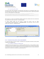
Administration Menu in GEoNetwork ................................................................................. 90
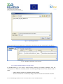
Import Metadata ................................................................................................................. 91
Metadata ............................................................................................................................. 91
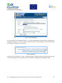
Edit metadata....................................................................................................................... 92
Save as Template ................................................................................................................. 92
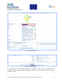
Validation report.................................................................................................................. 93
Options to create a new metadata ...................................................................................... 93
Adding template .................................................................................................................. 93
Choosing template............................................................................................................... 94
Insert Metadata as template ............................................................................................... 94
Metadata validated and inserted as template .................................................................... 95
D2.2 – Methodology specification for the harmonization of the available datasets 6
Fig 25.
Fig 26.
Fig 27.
Fig 28.
Fig 29.
Fig 30.
Fig 31.
Fig 32.
Fig 33.
Fig 34.
Fig 35.
Fig 36.
Fig 37.
Fig 38.
Fig 39.
Fig 40.
Fig 41.
Fig 42.
Fig 43.
Fig 44.
Fig 45.
Fig 46.
Fig 47.
Fig 48.
Fig 49.
Fig 50.
Fig 51.
Fig 52.
Fig 53.
Fig 54.
Fig 55.
Fig 56.
Fig 57.
Fig 58.
Fig 59.
Fig 60.
Fig 61.
Fig 62.
Fig 63.
Fig 64.
Fig 65.
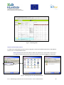
Example of a SCA source data model in Navarra, Spain ...................................................... 96
Example of a SCA source data model in Navarra, Spain ...................................................... 97
Matching table ..................................................................................................................... 98
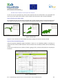
Selecting input file with Geoconverter ................................................................................ 98
Selecting output file with Geoconverter ............................................................................. 99
Matching fields .................................................................................................................. 100
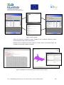
Example of a source data of SCA model in Navarra, Spain................................................ 100
Source data ........................................................................................................................ 101
Matching table ................................................................................................................... 101
Selecting input file ............................................................................................................. 102
Selecting output file........................................................................................................... 102
Exporting options............................................................................................................... 103
Matching fields .................................................................................................................. 103
Example of a source data of SCA model in Navarra, Spain................................................ 104
Geoserver web page .......................................................................................................... 105
Log in in Geoserver ............................................................................................................ 105
Edit Workspace in GeoServer ............................................................................................ 106
New data source in GeoServer .......................................................................................... 107
Map style in Geoserver ...................................................................................................... 108
Name and the title of the layer in Geoserver .................................................................... 109
Coordinate Reference Systems in Geoserver .................................................................... 109
Layer Preview in Geoserver ............................................................................................... 110
Showing the map in a web browser .................................................................................. 111
Metadata using UMN Mapserver ...................................................................................... 113
Layer Definition in UMN Mapserver .................................................................................. 114
Land Cover metadata......................................................................................................... 119
New Metadata Record in disy Preludio ............................................................................. 123
Metadata Creation in disy Preludio ................................................................................... 124
Bounding box in disy Preludio ........................................................................................... 125
Custom Coordinate reference system in disy Preludio ..................................................... 125
Approving in disy Preludio ................................................................................................. 126
Geobide plataform............................................................................................................. 129
Geoprocessing. .................................................................................................................. 130
Allowed Input and Output format ..................................................................................... 130
Configuration of the input format ..................................................................................... 131
Geocatalog ......................................................................................................................... 132
Reference coordinate system ............................................................................................ 132
Project type selection ........................................................................................................ 134
Choosing one INSPIRE XSD................................................................................................. 134
Choosing source database ................................................................................................. 135
Mapping elements ............................................................................................................. 135
TABLES INDEX D2.2 – Methodology specification for the harmonization of the available datasets 7
Table 1:
Table 2:
Table 3:
Table 4:
Table 5:
Table 6:
Table 7:
Table 8:
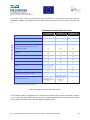
Data model transformation tools survey............................................................................. 39
Data remodelling process (NO source Data Model) ............................................................ 40
Data remodelling process (source Data Model) .................................................................. 41
Metadata transformation tools survey................................................................................ 43
Metadata remodelling process............................................................................................ 44
Quality process summary .................................................................................................... 46
Common parameters of a GetMap requests....................................................................... 50
WMS tools survey ................................................................................................................ 52
D2.2 – Methodology specification for the harmonization of the available datasets 8
1. INTRODUCTION Nowadays, Land Use (LU) and Land Cover (LC) information can be managed at national, regional or local level. This multilevel approach together with the inner complexity of the subject itself has resulted in a suite of datasets, not always compatible with each other. But in a context where environmental threats (for example; climate change, biodiversity loss, and food security) become more and more global, there is a need to better integrate various sources of information at various scales. So, we can conclude that there is an urgent need for harmonization and standardization of LC and LU information at various levels. Trying to give a solution to this situation, the HLANDATA project presents as one its specific objectives to make a proposal for the harmonization of LC and LU data and to demonstrate its validity for any of their possible uses and users through the development of some user oriented value‐added services. This document represents one of the required steps in order to obtain the needed harmonization. It attempts to give a comprehensive presentation of the HLANDATA harmonization methodology, understood as the sum of the tools and procedures that data providers could use for accomplishing the harmonization of the available LC and LU datasets. Although the scope and the objectives of the development of this methodology are defined according to what in the HLANDATA document of work is presented, those are always in line with the development and the implementation of the INSPIRE directive and with the consequences of its application. In this way, the HLANDATA harmonization methodology aims to be an example of best practice regarding the harmonization processes that all INSPIRE data providers will have to accomplish to be compliant with the implementing rules of the different themes. The following pages present a brief overview of the scope and objectives, continues with a description of some relevant harmonization principals and previous project researches in order to reuse the knowledge for the creation, as it is presented in the Chapter 4 General Approach for data Harmonization of this document, of the HLANDATA approach to the harmonization process ending with some interesting conclusions. Some ANNEXES have being attached to this document in order to simplify the access to the methodology presented in Chapter 5 HLANDATA Methodology without leaving relevant information out. D2.2 – Methodology specification for the harmonization of the available datasets 9
2. OVERVIEW 2.1. Normative References INSPIRE Technical Architecture Overview V1.2 INSPIRE DS‐D2.5, Generic Conceptual Model, v3.0 INSPIRE DS‐D2.8.I.9, Data Specification on Protected Sites ‐ Guidelines, v3.0 INSPIRE DS‐D2.7, Guides for the encoding of spatial data, v3.1 INSPIRE Metadata implementing rules: Technical Guides based on EN ISO 19115 / EN ISO 19119, v1.1 EN ISO 19107:2005, Geographic Information – Spatial Schema EN ISO 19108:2005, Geographic Information – Temporal Schema EN ISO 19108:2002/Cor 1:2006, Geographic Information – Temporal Schema, Technical Corrigendum EN ISO 19109:2005, Geographic Information – Rules for Application Schemas EN ISO 19113:2005, Geographic Information – Quality principles EN ISO 19114:2005, Geographic Information – Quality evaluation procedures (incl. Techn. Corrigend.) EN ISO 19115:2005, Geographic Information – Metadata (incl. Techn. Corrigend.) EN ISO 19123:2007, Geographic Information – Schema for coverage geometry and functions EN ISO 19131:2008, Geographic Information – Data Product Specification ISO/TS 19138:2006, Geographic Information – Data quality measures ISO/TS 19139:2007, Geographic Information – Metadata – Implementation Specification 2.2. General Definitions Terms and definitions necessary for understanding this document are defined in the INSPIRE Glossary [http://inspire‐registry.jrc.ec.europa.eu/registers/GLOSSARY]. Hereby some examples of those are presented: DATA HARMONIZATION: providing access to spatial data through network services in a representation that allows for combining it with other harmonised data in a coherent way by using a common set of data product specifications DATA PRODUCT SPECIFICATION: detailed description of a dataset or dataset series together with additional information that will enable it to be created, supplied to and used by another party [ISO/FDIS 19131 Geographic Information – Data Product Specification] METADATA information describing spatial data sets and spatial data services and making it possible to discover, inventory and use them [INSPIRE Directive] 2.3. Abbreviations CRS Coordinate Reference System CSW Catalog Web Service DM Data Model D2.2 – Methodology specification for the harmonization of the available datasets 10
DPS Data Product Specification DS Data Specifications DT Drafting Team EC European Commission GCM Generic Conceptual Model GML Geography Markup Language GMES Global Monitoring for Environment and Security GPL GNU General Public Licence INSPIRE Infrastructure for Spatial Information in Europe IR Implementing Rule IT Information Technology JRC Joint Research Centre LGPL GNU Library General Public License MD Metadata MS Member State MT Matching Table OGC Open Geospatial Consortium UML Unified Modelling Language WS Web Service WFS Web Feature Service WMS Web Map Service 2.4. Notation of Requirements and Recommendations To make it easier to identify the mandatory requirements and the recommendations for spatial data sets harmonization procedures in the text, they are highlighted and numbered. Requirements are shown using this style.
Recommendation 1
Recommendations are shown using this style.
D2.2 – Methodology specification for the harmonization of the available datasets 11
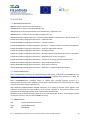
3. SCOPE During HLANDATA definition, interrelations between the different tasks and work packages were detected and analyzed in order to ensure a continuous and proper work flow. This work flow started with the accomplishment of WP1 tasks. Every data provider reported their available information regarding LC and LU and a diagnostic of the situation of data, related harmonization methodologies and user’s requirements was prepared. WP2 would use this review in order to, as part of Task 2.1. Harmonization, propose the HLANDATA Data Model and additionally the HLANDATA Metadata profile. This proposal development has being influenced by the presence of HLANDATA partners as experts in the Thematic Working Groups of Land Cover and Land Use. The process of data harmonization is addressed to make interoperable the information shared by the different data providers in the HLANDATA project. But, as it was said previously in the introduction, this process it is defined according to INSPIRE Directive principles, with the aim to meet its objectives of harmonizing, maintaining, and sharing information. This involvement in the development of the LC and LU DS has allowed HLANDATA to have a privileged overview of the European current situation regarding LC and LC and guarantees the adequacy of the HLANDATA proposal to the INSPIRE perspective and requirements. However, it is important to remark that HLANDATA, due to the timeframe of the project, will use the version 1.9 of the DS and that during the coming months possible minor changes may occur before the TWG work is finalised. But those are not expected to significantly change the HLANDATA harmonization methodology, only some minor adjustments could be done but they should not represent risk for future activities during the project. This document presents the HLANDATA Harmonization methodology. It represents the achievement of the Objective 2.2. To provide a methodology for the harmonization of the data. This objective is included in the Task 2.1. Harmonization proposal of the WP2, (figure 1) and is based on the results of the WP1 together with other previous harmonization initiatives such as EURADIN, NATURE SDI+, Humboldt and INSPIRE keeping in mind as further horizon the development of harmonized data sharing infrastructure. While working in the HLANDATA harmonization methodology it was noted that the main cost in complying with the INSPIRE Directive (and thus harmonising data) will be capacity‐building – the staff time taken to learn about INSPIRE, understand the requirements, and apply the specifications (i.e. the metadata profiles and data models) to the necessary datasets. This report is aimed at providing support for such data providers although it doesn’t remove completely the intrinsic complexity of the harmonization process that requires multidisciplinary experts to deal with the context and the technology. The methodology for the HLANDATA Land Use Land Cover data harmonization will be applied by all partners within the project, in order to carry out the harmonization of the available geographic information. It aims to be a guide to the procedures for the translation and remodelling of available datasets into the HLANDATA metadata profile and data model and to provide appropriated tools for it. It also gives guidance for the implementation of the generic web services which will be developed in Task 2.2. Development of the Common Data Sharing Infrastructure, further implemented in the Pilots in WP3. The agreement on the data formats and multilingual concepts to be applied by all partners and common methodology for the harmonization will also be established here. D2.2 – Methodology specification for the harmonization of the available datasets 12
Fig 1.
HLANDATA WP2 tasks, deliverables and interrelationships D2.2 – Methodology specification for the harmonization of the available datasets 13
4. GENERAL APPROACH FOR DATA HARMONIZATION 4.1. Data Integration: Types of Heterogeneity Dealing with data integration basically implies addressing two main types of heterogeneity: data heterogeneity and semantic heterogeneity. Data heterogeneity refers to differences in data in terms of data type and data formats and could be further split into the categories of Syntax and Structure, while semantic heterogeneity applies to the meaning of the data (Hakimpour and Geppert, 2001). −
Syntax heterogeneity refers to differences in formats. For instance there’s usually a loss of information when data from System A is exported as shapefile and converted to a mapinfo file to be imported into System B. −
Structure heterogeneity is related to differences in schemas (formalised descriptions of conceptual data models). For instance Schema A foresees one attribute for address, Schema B offers three) −
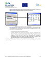
Semantic heterogeneity is related to the differences in intended meaning of terms in specific contexts. The object “forest” as modelled by a regional planner might have the meaning of natural recreation area (accessibility, sports facilities, picnic areas, etc.) whereas a forest ranger might understand the term from a timber industry viewpoint (kind and amount of wood, schedule for lumber, potential customers, etc.) With the foundation of the Open Geospatial Consortium (OGC)1 in 1994, solutions to overcome the problems of syntactical interoperability were initiated. The idea behind the joint development of de‐
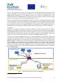
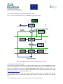
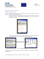
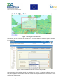
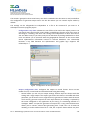
facto Web Service standards was to use the Internet as ubiquitous communication platform via which the different systems were connected and to define standardised interfaces for the exchange of spatial data. OGC Specifications like OGC WMS, WFS, CSW or GML are well known and widely established. In order to transfer the de‐facto industry standards into de‐jure standards, OGC and ISO have been cooperating for several years. The problem with semantic interoperability is that the differences on the level of data models are generally neglected. Users are very well able to access data from different sources, but without further information it is often difficult to judge what further steps are necessary to fully integrate the different sources since there’s only limited information about the underlying data models i.e. the structure available. The following figure illustrates the problem: three different WFS were accessed with GeoMedia and displayed without any further editing. The results are not easy to interpret. Fig 2.
Unedited WFS integration GI 1
OGC: Open Geospatial Consortium: http://www.opengeospatial.org D2.2 – Methodology specification for the harmonization of the available datasets 14
The technological obstacles of making different systems communicate with each other in a coherent way – i.e. the syntactical or structural interoperability – can be addressed by means of standardised web service interfaces like WMS or WFS among others. But the next step of semantic interoperability really ensures that the concept or idea of a modelled real world object is commonly understood and shared. ‘Semantics’ deals with aspects of meaning as expressed in a language, either natural or technical such as a computer language, and is complementary to syntax which deals with the structure of signs (focusing on the form). In the area of distributed data sources and services, semantic interoperability refers to the ability of systems to exchange data and functionalities in a meaningful way. Semantic heterogeneity occurs when there is no agreement on the meaning of the same data and/or service functionality. Semantic interoperability ensures that the requester and provider of services and data have a common understanding of the meaning of the services or data they exchange (Heiler, 1995). Data creation happens in a context or in an application domain where concepts and semantics are clear to the data creator, either because they are explicitly formalised or because they are naturally applied due to a yearly experience. But with distributed data resources this context is missed and unknown to the end user. This means that, in order to achieve semantic interoperability, semantics should be formally and explicitly represented (Kuhn, 2005). Semantic heterogeneities may be classified in two macro‐categories: −
Naming heterogeneities (when different words/expressions are used for the same concept) −
Conceptual heterogeneities (when different concepts are expressed by the same words/expressions/symbols) (Kuhn, 2005). Application schemas and metadata may be considered as a means to provide information about the context in which data have been created, but schemas do not provide explicit semantics of their related data and metadata values are not machine‐readable (Klien, 2007). There are several ways (controlled vocabularies, taxonomies, thesaurus, ontologies) to make explicit the semantics of a dataset or of an application domain; the approaches vary in terms of complexity, formalism, and amount of information they provide. −
Controlled vocabulary: a controlled vocabulary is a list of terms that have been enumerated explicitly (controlled means that there is registration authority responsible for it). Controlled vocabularies solve the problems of homonymy (a group of words that share the same spelling or pronunciation (or both) but have different meanings), synonymy (different words with identical or at least similar meanings) and polysemy (is a word or phrase with multiple, related meanings) by ensuring that each concept is described using only one authorized term and each authorised term in the controlled vocabulary describes only one concept2: when different terms are used to mean the same thing, one of the terms is identified as preferred and the others are listed as aliases. An example of controlled vocabulary is the DCMI Type Vocabulary used in Dublin Core3. 2
http://en.wikipedia.org/wiki/Controlled_vocabulary http://dublincore.org/documents/dcmi‐type‐vocabulary/index.shtml 3
D2.2 – Methodology specification for the harmonization of the available datasets 15
−
Taxonomy: It’s the science and methodology of classifying organisms based on physical and other similarities. Taxonomists classify all organisms into a hierarchy, and give them standardized Latin or Latinized names. −
A thesaurus is the vocabulary of a controlled set of terms selected from natural language and used to represent, in summarized form, the subject of documents. It is formally organized so that a priori relationships between concepts (namely those are part of common and shared frames of reference as broader and narrower relationships) are made explicit [ISO 2788‐1986]. −
The term ontology is often used to mean different things, such as vocabularies, thesauri, taxonomies, schemas, data models, and formal ontologies. A formal ontology, as defined in (Studer, 1998), is “… an explicit formal specification of a shared conceptualization. A ‘conceptualisation’ refers to an abstract model of some phenomenon in the world by having identified the relevant concepts of that phenomenon. A formal ontology is expressed in an ontology representation language (e.g. RDF4, OWL5, etc.), which is machine‐readable: this means that reasoning software can apply inference rules in order to integrate different ontologies. 4
http://en.wikipedia.org/wiki/Resource_Description_Framework http://en.wikipedia.org/wiki/Web_Ontology_Language 5
D2.2 – Methodology specification for the harmonization of the available datasets 16
4.2. Data Harmonization: Concepts and Definitions In order to decide about the suitable methods and workflows, it is important to understand some basic terminology regarding data harmonization. Longley et al. (2005) suggest that there are four different levels of abstraction of the world within GIS, (conceptual model, logical model or physical model) as illustrated in Figure 3. Fig 3.
Levels of abstraction relevant to GIS data models (Longley et al, 2005) Reality includes all phenomena in the real world including those objects not perceived by humans. The Conceptual Model is a human oriented model of the world consisting of objects that a specific human considers relevant to a specific domain. It can be argued that there is only one reality, whereas there are almost as many conceptual models as there are people. . The Logical Model is used to explore the domain concepts, and their relationships, and is often expressed as class models in UML. This stage is significant because it is the logical model which will be affected by the aggregation and degradation of data as it is harmonised. Tasks 2.1 of the WP2, has been concerned with this step during the development of the proposal for the harmonization of the LAND Use and Land DATA geographic information. The Physical Model is used to design the internal schema of a database, depicting how the physical data is stored on a machine, i.e. the data tables, the data columns of those tables, and the relationships between the tables stored as flat files or databases. This means that the physical model is of low significance because the project is not concerned with the concrete storage of datasets in machines. In our case, the data and data models made available by the providers illustrate a great level of Heterogeneity. The data harmonization process will address the homogenization and organization of that initial information giving it consistency and interoperability. Then, it is possible to create the common data sharing infrastructure allowing access to harmonized information. D2.2 – Methodology specification for the harmonization of the available datasets 17
The next sections present an overview of commonly used definitions and concepts to ensure an unambiguous understanding of “Data harmonization”. Nevertheless, the concept of Data Harmonization has been defined from different perspectives which apparently are considering very different aspects. The fact of having different definitions and concepts illustrates perfectly the importance of semantics: the information contained in a message can only be interpreted correctly if both receiver and sender of the message share a common view on the message. Within the INSPIRE process, a definition for data harmonization was also developed and states that, data harmonization is the “process of developing a common set of data product specifications in a way that allows the provision of access to spatial data through spatial data services in a representation that allows for combining it with other harmonised data in a coherent way6. In the next sections the “data harmonization” definitions given by related European projects and by HLANDATA are presented. 4.2.1.Related Projects Quite a number of international / EU projects are dealing with data harmonization. In order to avoid a duplication of efforts and to increase the synergies between closed and existing (research) projects, this report also includes references to projects like PLAN 4 ALL, EURADIN, NATURE SDI+ and HUMBOLDT . PLAN 4 ALL Plan4all deals with the harmonization of spatial planning data according to the INSPIRE Directive based on existing best practices in European regions and municipalities and the results of current research projects. The Plan4all project contributes to the standardization in the field of spatial data from spatial planning point of view. Its activities and results are reference material for INSPIRE initiative; especially for data specification. Plan4all is focused on the following seven spatial data themes as outlined in Annex II and III of the INSPIRE Directive: land cover, land use, utility and governmental services, production and industrial facilities, agricultural and aquaculture facilities, area management/restriction/regulation zones and reporting units and natural risk zones. The main project objectives are to promote Plan4all and INSPIRE in countries, regions and municipalities; to design spatial planning metadata profile; to design data model for selected spatial data themes related to spatial planning; to design networking architecture for sharing data and services in spatial planning; to establish an European portal for spatial planning data and to deploy data and metadata on local and regional level. A detailed state of art analysis at the beginning of the project provides basic information on best practices, existing data models and metadata profiles, user requirements as well as methodologies and tools for data harmonization. The regional deployment is focused mainly on deployment of metadata systems with the Plan4all profile, and on the deployment of network services according to the requirements of content providers. An important part of deployment is the implementation of transformation services, which supports transformation of data from existing models into data following the designed conceptual models. The developed data models are at conceptual level which contains all information elements that are classes with their attributes and relationships between classes. The Land cover data model is used as guideline and example for the other data models. UML is used to specify the data models in diagrams. Pan‐European deployment is focused on deployment of a central geoportal with client 6
This includes agreements about coordinate reference systems, classification systems, application schemas, etc.” (INSPIRE D2.3, p.6). D2.2 – Methodology specification for the harmonization of the available datasets 18
applications and network services like discovery and portrayal services. An important role plays multilingual search for data and common portrayal rules. The Plan4all geoportal provides the means to search for spatial data sets and spatial data services with regard to spatial planning. It allows the user to view and download spatial data sets (subject to access restrictions) and related metadata. CurrentlyPlan4all standards (metadata profile, data models and networking architecture) are being validated and tested by experts on local and regional level. The present project results and deliverables are available on the Plan4all website7. Fig 4.
Plan4All work plan diagram EURADIN From EURADIN Project perspective the concept of harmonization looks at proposing a solution to achieve their interoperability of address information and thus facilitating the effective access, reuse and exploitation of that content, which will promote the creation of new added value products and services across Europe. It considers harmonising as part of the address data flow process according to the definition “Harmonising is a process to make data compliant to agreed specifications” (Cook Book on Data Flow – Deliverable 5.1 Report) EURADIN consortium have been strongly involved in the testing process of INSPIRE Address theme, analysing the specifications and providing comments and suggestions to better adapt to the current use of address data. Finally, at the end of this testing the suggestions from EURADIN partners have facilitated the proposal of a data model specification closer to the real data. Based on the project tasks and interacting with the INSPIRE data specifications draft, they were able to match the existing INSPIRE framework to the address topic, delivering a technical proposal on 7
http://www.plan4all.eu./ D2.2 – Methodology specification for the harmonization of the available datasets 19
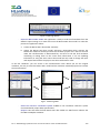
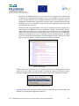
Data to the European Commission as obtaining of the Harmonised Address Data Model. This technical proposal was the core result for the project, as it was thought as strongly adherent to the INSPIRE Data Specification v2.0 on Addresses and it was ready for experimentation in the implementation phase of EURADIN, during which the 3.0 Version appears and the consortium agreed to use it as reference version for implementing Gazetteer services. The technical proposal prepared by EURADIN partnership was able to add data requirements coming from the validation to the data requirements already addressed by the INSPIRE Data Specification v3.0 of the Address TWG. It also provided suggestions about a better integration and harmonization of the Address topic with other INSPIRE themes, in consideration that EURADIN project has a privileged view, as responsible of immediate implementation of a gazetteer service for addresses. HUMBOLDT Humboldt is focusing on providing a software framework for data harmonization and services integration that supports all kinds of users (experts as well as laymen) in data harmonization efforts. The HUMBOLDT definition of data harmonization is therefore user‐centric: “creating the possibility to combine data from heterogeneous sources into integrated, consistent and unambiguous information products, in a way that is of no concern to the end‐user” (HUMBOLDT 2006 –A3.5 D1). “The main goal of the HUMBOLDT project is to enable organisations to document, publish and harmonise their spatial information. The software tools and processes created will demonstrate the feasibility and advantages of an Infrastructure for Spatial Information in Europe as planned by the INSPIRE initiative, meeting at the same time the goals of Global Monitoring for Environment and Security (GMES)” 8. The idea of having a comprehensive analysis of the existing source data models and of investing effort in defining a target data model that meets the needs of certain application domains is also followed within the HUMBOLDT project. This two‐fold approach is best depicted in the following image that was also presented during the INSPIRE 2008 conference in Maribor, Slovenia (GIGER 2008): Fig 5. Data harmonization processes in HUMBOLDT 8
www.esdi‐humboldt.eu D2.2 – Methodology specification for the harmonization of the available datasets 20
The blue frame represents the technical processes necessary to transform data from various sources into a given / defined target. The HUMBOLDT Framework shall support these technical processes by means of various tools and methods. The second part of the harmonization processes can be headlined with “target definition”. Prerequisite is profound understanding of the available data sources. There are two ways how to define a target – depending on the respective users need. Option A is to define a target or a common schema for a certain data theme as it happens within INSPIRE and the data specifications for the INSPIRE ANNEX I – III themes. This kind of data model specification is based on decisions (including also political decisions). Option B is to define a target model for the certain needs of an application domain. Here relevant data sources need to be combined from a variety of themes and are designed to fit best to the specific application domain. NATURE‐SDIplus The NATURE‐ SDIplus Document of Work (Dow) emphasizes about the need to harmonise and make data interoperable and consistent. Three main aspects can be considered: −
The “harmonization” of spatial data sets. This means the ability of data to be compatible and implies the adoption of common rules in application schemas, co‐ordinate reference systems, classification systems, identifier management, etc. from different points of view. −
The “interoperability” of the spatial data sets. This means the ability of the data to be combined and interact and implies the adoption of a common framework and network services that enables them to be linked up from one to another. −
The “consistency” between spatial data sets. This means that the representations of different objects which refer to same location, or of the same objects at different scales, or of objects spanning the frontier between different MS, are coherent. In practice it means that data sets coming from different levels of authority or from different countries can be easily used together by any type of user. 4.2.2. HLANDATA HLANDATA project will study the different harmonization initiatives carried out up to the moment, and others being carried out at present moment, both from the data model and data categorization harmonization perspectives. In parallel, the potential Land Use and Land Cover datasets Users’ needs will be assessed. Taking into account the results of these activities, a Land Use and Land Cover harmonization proposal will be developed, which will be the base for the development of specific web services for different application areas of the Land Cover and Land Use datasets. At this point, the newly developed web services will be used for the development of 3 Pilot Projects in 3 different application areas, which will be used to validate the harmonization proposal made: −
PILOT 1: Land Use‐ Land Cover Data analysis System for intermediate‐level users −
PILOT 2: Harmonized and Interoperable Land Information Systems −
PILOT 3: Stratification of waste dumps The assessment of the results of these pilot projects and the related Land Use models will lead to the generation of a harmonized Land Use Classification scheme and a methodology for the harmonization of the Land Use datasets. D2.2 – Methodology specification for the harmonization of the available datasets 21
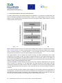
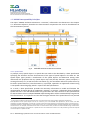
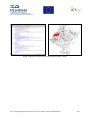
4.3. INSPIRE Interoperability Principles The report “INSPIRE Technical Architecture – Overview”, referenced in this document in the Chapter 2.1. Normative Reference, describes the harmonization components that need to be addressed in this harmonization process. Fig 6.
INSPIRE technical architecture overview 4.3.1. Spatial Data In principle, every spatial object in a spatial data set needs to be described by a data specification specifying the semantics and the characteristics of the types of spatial objects in the data set. The spatial object types provide a classification of the spatial objects and determine among other information the properties that any spatial object may have (be they thematic, spatial, temporal, a coverage function, etc.) as well as known constraints (e.g. the coordinate reference systems that may be used in spatial data sets). This information is, in principle, captured in an application schema using a conceptual schema language, which is a part of the data specification. As a result, a data specification provides the necessary information to enable and facilitate the interpretation of spatial data by an application. However, in practice, a substantial share of existing spatial data sets is not well documented. Only spatial data sets that conform to data specifications for Annex themes that are adopted INSPIRE Implementing Rules will be considered fully integrated in the infrastructure9. It is important to note that the logical schema of the spatial data set may and will 9
It may also be considered in how far the following cases are understood as part of the European spatial data infrastructure: Data specification exists: Spatial objects that are not covered by one of the INSPIRE data specifications, but for which a full data specification has been developed by a community or project and which has been published in an appropriate register in the infrastructure. Limited documentation: Spatial objects or just map layers that are not or not fully described by any data specification which is registered in the infrastructure. For example, some data files for which no documentation exists, but which are made available though a View Service. The minimum documentation requirement for a spatial data set in the infrastructure is that it has to be possible to generate the required service descriptions to publish the data. D2.2 – Methodology specification for the harmonization of the available datasets 22
often differ from the specification of the spatial object types in the data specification. In this case, and in the context of real‐time transformation, a service will transform queries and data between the logical schema of the spatial data set and the published INSPIRE application schema on‐the‐fly. This transformation can be performed e.g. by the download service offering access to the data set or a separate transformation service. The Drafting Team "Data Specification" develops the initial drafts that specify the framework for developing the Implementing Rules for the data specifications for the Annex themes. The conceptual modelling framework standardised in the ISO 19100 series of International Standards provides the basis for these developments. In order to support the interoperability requirements given in the Directive, the data specifications will have to be the result of a harmonization process based on existing data sets and, where available, requirements from environmental applications. A number of individual aspects, called data harmonization components, have been identified that need to be addressed in this harmonization process: −
Principles: The principles cited in recital (6) of the Directive are considered to be a general basis for developing the data harmonization needs. −
Terminology: A consistent language, managed in a multilingual glossary, has to be used throughout INSPIRE. −
Reference model: A common framework for the technical arrangements in the data specifications is required to achieve a consistent structure across the individual themes. −
Rules for application schemas and feature catalogues: Application schemas and feature catalogues provide the formal specification of the spatial data and promote the dissemination, sharing, and use of geographic data through providing a better understanding of the content and meaning of the data. Across the individual themes common rules are required to achieve the required coherence. −
Spatial and temporal aspects: While the reference model specifies an overall framework, this aspect deals with the spatial and temporal aspects in more detail, for example, the types of spatial or temporal geometry that may be used to describe the spatial and temporal characteristics of a spatial object. −
Multi‐lingual text and cultural adaptability: Rules for the support for multi‐lingual information in data specifications. −
Coordinate referencing and units of measurement model: Specification of the conceptual schema for spatial and temporal reference systems as well as units of measurements – including the parameters of transformations and conversions. −
Object referencing modelling: Rules for the specification of the spatial characteristics of a spatial object based on already existing spatial objects, typically base topographic objects, rather than directly via coordinates. −
Data transformation model / guidelines: Rules for the transformation from an existing data model to an INSPIRE application schema and vice versa. Transformations are required for data and for queries. D2.2 – Methodology specification for the harmonization of the available datasets 23
−
Portrayal model: Schema for portrayal rules for data according to a data specification. −
Identifier management: Specification of the role and nature of unique object identifiers based on existing national identifier systems. −
Registers and Registries: See chapter 5 of report “INPIRE Technical Architecture – Overview”. −
Metadata: Guides for documenting metadata for data sets as well as spatial objects on the levels discovery, evaluation, and use. −
Maintenance: Guides for the maintenance of spatial data sets within INSPIRE. −
Data & information quality: Guides for the publication of quality information, e.g. on completeness, consistency, currency and accuracy. −
Data transfer: Guides for encoding data based on the conceptual model in the data specification. −
Consistency between data: Guides for the consistency between the representation of the same entity in different spatial data sets (for example along or across borders, themes, sectors or at different resolutions). −
Multiple representations: Best practices for the aggregation of data across time and space and across different levels of detail. −
Data capturing rules: Guides which entities are to be represented as spatial objects in a spatial data set. For INSPIRE data specifications it is in general not relevant, how the data is captured by the data providers. −
Conformance: Rules for the description of abstract conformance tests in data specifications. 4.3.2. Metadata A spatial data set is described by data set metadata providing information supporting the discovery –
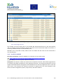
and to a certain extent also the evaluation and use – of spatial data sets for specific usages. Service metadata provides basic information about a service instance to enable the discovery of spatial data services. The description of a service includes the service type, a description of the operations and their parameters as well as information about the geographic information available from a service offering. The Drafting Team "Metadata" developed the Implementing Rule of data sets and services metadata for discovery. To support discovery a search will in general require support for keywords or other simple search criteria describing key characteristics of the resource (e.g. about the topics or spatial object types that are covered by the spatial data set)10. In addition, search criteria have to support searching based on spatial and temporal extents. Metadata must be kept consistent with the actual resource. I.e. a change in the resource has to result in an (automatic or manual) update of the associated metadata document describing the resource. 10
An objective for the future might be to support ontology in the discovery service (or its clients) to support searches on related terms where possible relations between two vocabularies may include identity, specialisation, aggregation, exclusion, etc. However, this is a research topic and out‐of‐scope for INSPIRE for at the moment. D2.2 – Methodology specification for the harmonization of the available datasets 24
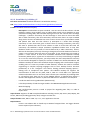
5. HLANDATA METHODOLOGY Taking as starting point the different formats and data model used by the HLANDATA data providers the HLANDATA methodology will start by guiding the transformation and remodelling of this data into harmonize LU/LC data. This part of the harmonization it will be called HLANDATA Harmonization Process. It includes also the harmonization of the metadata into the HLANDATA metadata profile. The Metadata profile it has been worked out in WP2 together with the definition of the LU and LC data model in close relationship with the TWG of LC and LU. Fig 7.
HLANDATA harmonization processes D2.2 – Methodology specification for the harmonization of the available datasets 25
The HLANDATA harmonization methodology will allow the creation of an accessible repository of harmonized data. The final objective is to be able to share HLANDATA and/or INSPIRE compliant datasets and metadata from the different partners on the harmonized common data sharing infrastructure. HLANDATA Harmonization Process provides not only a clear overview of the recommended steps for accomplishing the harmonization of data and metadata but also an overview of the different available tools and techniques in order to make this process easy to follow for the experts involved in. The transformation tools needed for accomplishing this harmonization can be chosen by each data provider. Tracasa and CEIT ALANOVA as technology providers will offer, among others, no cost products to support the harmonization efforts within HLANDATA project. Different tools, provided by the HLANDATA partners or external applications, will be presented in Chapter 5.1. HLANDATA Harmonization Process and also a more detailed explanation can be found in the Annex III. Once the harmonization process is presented, the second part of the HLANDATA methodology, the HLANDATA Implementation of the generic web services will be offered. This document includes in Chapter 5.2. HLANDATA Implementation of the Generic Web Services and Annex II all the information required in order to be able to easily publish the harmonised data during the development of Task 2.2. Design, development and validation of the harmonized data sharing infrastructure. In order to achieve the objectives included in the HLANDATA Dow regarding task 2.2, Web Map Services have being defined as the minimum generic web services required to establish the common harmonized data sharing infrastructure. Therefore a description of its main characteristics, tips for its implementation and some tools to will be presented in this part of the HLANDATA methodology. D2.2 – Methodology specification for the harmonization of the available datasets 26
5.1. HLANDATA Harmonization Process As has been explained before, the data custodians have very heterogeneous data, and some of them with no associated metadata. The harmonization process will be focused in: −
Previous study and comparison of available data and metadata with the HLANDATA data model and metadata profile. −
Transform or create datasets and metadata according to the HLANDATA data model and metadata profile. A set of two matching tables for data and another two for metadata will be prepared for helping partners to find the similarities between their source information models and HLANDATA data model and metadata profile. These matching tables will relate the attributes and fields of the source data model or metadata profile with those of the final HLANDATA data model and metadata profile. They could be a very useful instrument to achieve the data and metadata harmonization, as we explain in section 5.1.2.1. Matching Tables. The knowledge about how conceptual data models are encoded into implementation schemas and how the mapping on the conceptual level between source and target does look like, are a prerequisite for this process. Therefore, the matching tables produced by the partners in WP2 during the development of the data model are an essential input for the harmonization work. Once the relationships between the actual and targeted data model and metadata profile are clarify the transformation process will take place. The needed transformation tool can be chosen by each data provider. Tracasa and/or CEIT ALANOVA as technology providers will offer no cost products to support the harmonization efforts within HLANDATA. A first presentation of these tools can be found in section 5.1.2. HLANDATA Harmonization Tools and Techniques. For examples and detailed information please go to annex II and III. As the result of this transformation all the data and metadata will be harmonized and will be ready for being for being publish in the common data sharing infrastructure. This implementation process will be described in Chapter 5.2. HLANDATA Implementation of the Generic Web Services As a summary of this section it can be said that the HLANDATA harmonization process is expected to provide the tools and procedures that will make easier the transformation processes required for obtaining harmonized data. These tools and procedures for the transformation presented in the next sections include: −
−
Step by step guides to perform a correct harmonization depending on the tools and input data models and metadata profiles involved. Two separated guide will be developed: o
Data harmonization guide. o
Metadata harmonization guide. Harmonization tools and techniques o
Matching tables o
Tools for transformation of data models and metadata profiles, with a study of which tool could be the most suitable depending on the data providers’ Data Model and metadata profile. D2.2 – Methodology specification for the harmonization of the available datasets 27
−
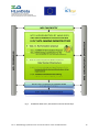
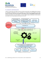
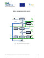
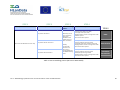
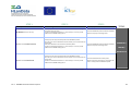
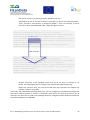
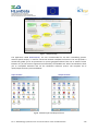
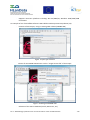
Quality checks and aspects to consider in order to assure that the harmonization process is well performed and documented. 5.1.1. Step by Step guides During this section the guides for accomplishing Data and metadata harmonization are presented. Each of these guides is based on a list of steps that can be easily followed. These steps are explained in detail helping the expert in church of the harmonization, giving possible tips, answers, recommendations and requirements. Each guide presents at the beginning a complete process diagram containing the symbols described in the following figure: Beging and End of the Harmonization process
Guiding
questions
Guiding questions
Previous
procedures
Previous procedures
Procedures
Procedures included in the harmonization
Step 3
Steps number and limits
Work flow direction
Fig 8.
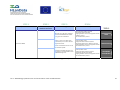
Elements presented in the step by step guide summary diagram For facilitating the comprehension of these guides special writing style is used in the coming pages until section 5.1.2. HLANDATA Harmonization Tools and Techniques. The guides presented during this entire document could be considered as the core of the document. D2.2 – Methodology specification for the harmonization of the available datasets 28
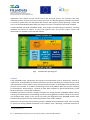
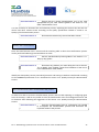
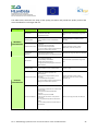
DATA HARMONIZATION GUIDE
Identify source
data model
Start Harmonisation Process
Without
Data Model
HLANDATA
Data Model
Data Model?
Create the
Matching Table
Fill Matching
Table
Matcheable?
Choose
Transformation Tool
and Document
Create a simple
GeoData Structure
NO
Perform
Transformation
Document
Store
Tranformation Rules
and Document
Finish Harmonisation Process
Fig 9.
Data Harmonization process diagram D2.2 – Methodology specification for the harmonization of the available datasets 29
STEP 1
Identify source data model Once our available LC and/or LU data is identified, in order to be able to harmonize it, the data providers have to know how it is organized and stored. A guiding question is added at this point: Is there a LU or LC data model? The purposed possible answers are: ¬
There is no data model: this means that data either there is no data or it doesn’t have relation between the graphic and alphanumeric information or the subject of the data is non of these two (LU and LC) It will be necessary to create a simple11 data model structure.
¬
There is a data model: Data presets relationship between the graphic and alphanumeric information, and this information is related to LU or LC. Then, the information is ready to be filled in the matching table. The closer the source model is to the target model the easier to perform the transformation will be. ¬
And if the data model is compliant with the LU or LC HLANDATA data model, it can be considered that the harmonization process is done, and this harmonization process would be finished. STEP 2
Create a simple Geodata structure A basic Geographic Information System structure must be created using a Desktop GIS tool. Spatial and alphanumeric information must be linked by any data model. The suggested tools for this task are not included in the list of tools of section “5.1.2.2. Data Transformation Tools” but some are here presented: −
Open Source: gvSIG, uDIG, Kosmo −
Licensed: Mapinfo Professional, Geomedia Professional, ESRI ArcGIS, Autodesk Map. 11
In this case “simple” means a structure that contains spatial information (area, line or point) with some related alphanumeric information. D2.2 – Methodology specification for the harmonization of the available datasets 30
STEP 3
Fill the data matching table Considering the matching table a helpful tool to transform the data, in this step we will compare and match up the attributes of the source data model with their correspondence in the target HLANDATA data model. It is necessary to fill every mandatory field of the HLANDATA model. Recommendation 1
Search into your source data all the information you can
match with the target data model.
Create new attributes for the rest of the mandatory fields
Document the process by listing gaps and problems By matching the conceptual model of the supplied data to the HLANDATA model, it is possible to identify possible gaps in the HLANDATA data model. Detecting gaps it is also a prerequisite to see if the current schemas of the data providers address all mandatory elements (objects and attributes) of the HLANDATA data model. The Matching Table should be used for documenting this comparison by adding comments related to each element on the column “Remarks”. Recommendation 2
It will be very important to identify unmatchable attributes and
document them. Also, it will be useful to provide feedback to the
Data Specification Drafting Teams, so they can consider these
issues during the development of the DS.
STEP 4
Choose a tool to perform the transformation and document the process To perform the data structure and storage transformation, any licensed or open source transformation tool will be chosen. Section 5.1.2.2. Data Transformation Tools introduces several tools and makes a comparative study. This chapter was written to facilitate the choice of the users between the different transformation tools. D2.2 – Methodology specification for the harmonization of the available datasets 31
Recommendation 3
Ensure that the chosen transformation tool is the most
appropriated for your case. See the guides in the section 5.1.2.2.
Data Transformation Tools
It is also necessary to document this tool selection process, explaining the reasons why the tool was chosen and other relevant issues according to the quality specification related in section 5.1.3. Quality of the harmonization process. Recommendation 4
Document the reasons why the tool has been chosen.
Perform the transformation Once the transformation tool is chosen and the matching table is done the transformation process can be performed obtaining harmonised data as result. Recommendation 5
See the transformation process guides in the section 5.1.1.
Step by step guides
Recommendation 6
Document any problem you meet during the use of the tool.
Try to identify if the problem comes from limitations of the tool or
from characteristics of the dataset.
Identify the data quality control procedures/protocols and testing on GIS data transformed according to the HLANDATA specification as it is introduced in section 5.1.3. Quality Control for Harmonization Process. Store Transformation Rules and document the process In order to be able to reuse the transformation process and to avoid repeating or configuring again some of the steps, it will be very useful to store all transformation rules and configuration issues and to document them following the suggestions of the section 5.1.3. Quality Control for Harmonization Process. Recommendation 7
Store the Transformation Rules or configuration info needed
to accomplish the transformation process and document the
important issues of the process.
D2.2 – Methodology specification for the harmonization of the available datasets 32
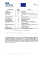
METADATA HARMONIZATION GUIDE
Identify source
metadata profile
Start Harmonisation Process
Step 1
NatureSDIplus
Metadata Profile
No Metadata
Metadata?
Any metadata
profile
Fill Matching
Table
Matcheable?
Step 2
Create the
Matching Table
NO
Document
Create or Update
Metadata
Store
Tranformation Rules
and Document
Finish Harmonisation Process
Step 3
YES
Choose
Metadata Tool
and Document
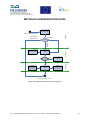
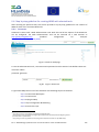
Fig 10. Metadata Harmonization process diagram D2.2 – Methodology specification for the harmonization of the available datasets 33
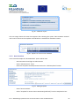
STEP 1
Identify and characterize a source metadata profile Once our available LC and/or LU metadata is identified, in order to be able to harmonize it, the data providers have to know its level of development and if it matches with LU or LC metadata HLANDATA profile. A guiding question is added at this point: Is there any metadata for the LU and/or LC data? ¬
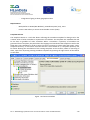
If there is no metadata, or if there is metadata but the profile doesn’t match with HLANDATA metadata profile: It is necessary to create or modify the metadata using HLANDATA profile and the matching table.
¬
If the metadata matches with the HLANDATA profile, it can be consider that harmonization process is done, and this harmonization process would be finished. STEP 2
Fill the metadata matching table Considering the matching table a helpful tool to transform the metadata, in this step we have to compare and to match up the elements of the source metadata profile with their correspondence in the target HLANDATA metadata profile. It is necessary to fill every mandatory field of the HLANDATA profile. Recommendation 1
Search into your source metadata all the information
matching with the target profile.
Create new metadata for the rest of the mandatory fields.
Document the process by listing gaps and problems By matching the conceptual model of the supplied metadata with the HLANDATA profile, it is possible to identify possible gaps in the HLANDATA metadata profile. Detecting gaps it is also a D2.2 – Methodology specification for the harmonization of the available datasets 34
prerequisite to see if the current schemas of the data providers address all mandatory elements (objects and attributes) of the HLANDATA metadata profile. The Matching Table should be used for documenting this comparison by adding comments related to each element on the column “Remarks”. Recommendation 2
It will be very important to identify unmatchable attributes and
document them. Also, it will be useful to provide feedback to the
Data Specification Drafting Teams, so they can consider these
issues during the development of the DS..
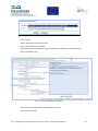
STEP 3
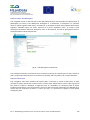
Choose a tool to edit or create metadata and document the process To perform the filling of the metadata structure and the storage of the metadata is necessary to choose a licensed or open source metadata editor tool. In section 5.1.2.3. Metadata Transformation Tools, several tools are introduced in order to ease partners’ choice. It is also important to review the results of the comparative survey of Metadata Tools. Recommendation 3
Ensure that the chosen metadata editor tool is the most
appropriated for your case. Please, take into account your source
metadata profile and use the results of the Metadata Tool Survey.
It is also necessary to document this tool selection process, including the reasons why the chosen tool is the most appropriated and other relevant issues according to the quality specification related in section 5.1.3. Quality of the harmonization process. Recommendation 4
Document the reasons why the tool has been chosen.
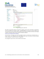
Create or Update metadata With the source metadata, the metadata editor tool and the matching table, the transformation can be performed and the HLANDATA harmonised metadata obtained. Recommendation 5
See the guides
Transformation Tools
in
the
section
5.1.2.3.
Metadata
D2.2 – Methodology specification for the harmonization of the available datasets 35
Recommendation 6
Document any problem you meet during the use of the tool.
Try to identify if the problem come from limitations of the tool or
from characteristics of the metadata.
Identify the metadata quality control procedures/protocols and testing on metadata transformed according to the HLANDATA specification as it is introduced in section 5.1.3. Quality Control for Harmonization Process. Store Transformation Rules and document the process In order to be able to reuse the process and to avoid repeating or configuring again some of the steps, it will be very useful to store all transformation rules and configuration issues and to document them following the suggestions of the section 5.1.3. Quality of the harmonization process. Recommendation 7
Store the Transformation Rules and the needed configuration
info to accomplish the transformation process and document the
important issues of the process.
D2.2 – Methodology specification for the harmonization of the available datasets 36
5.1.2. HLANDATA Harmonization Tools and Techniques 5.1.2.1. Matching Tables In this section the process followed for the creation of the matching tables and the value of its use are explained. In general terms a matching table is the way to establish the relation between source information and a target information model. It is, therefore, a useful tool for data providers in order to realize how close the input data or metadata is to the HLANDATA requirements. During the development of the HLANDATA data model, and after several teleconferences and discussions, a first set of matching tables for LU and LC were created and distributed to all the data providers supplying a first overview of the harmonization possibilities of the consortium. Partners reached an agreement to use INSPIRE Data Specification v1.9 for LC and LU (Annex III) as the target data model in the HLANDATA project, although assuming these models could vary in time. The final version of matching tables will be composed by two excel file, one for metadata and one for data model. Each excel sheet is divided in two main areas. On the left side is the INSPIRE LU or LC Data model or metadata profile. On the right side is the provided source information. This information has to be in the original language of the provider and in English. There is also a column “Remarks” that should be used for documenting the important issues found during the matching process. In the same way as for the Metadata, Data matching table will be an excel file with two sheets: Land Use and Land cover. The final version of the matching tables for data and metadata will be attached to this document when the version 1.9 of the specifications will be presented. D2.2 – Methodology specification for the harmonization of the available datasets 37
5.1.2.2. Transformation Tools Once the matching table is completed, the source dataset is related with the target HLANDATA information. Then it is possible to use the transformation tools to perform data harmonization. These transformation tools are the applications that allow creating the output data model with the proper format, attributes, coordinate system, units, etc. Data Transformation Tools In this section some tools that can be used in the data transformation are described. These tools allow data providers to create or transform their own data into HLANDATA data models. In order to perform a data tools classification we have made a survey with some questions we consider useful for helping in the process of choosing the appropriate tool. The description of these questions is as it follows: Allowed input /output formats The input formats that the tool supports Read input data Only data attributes are read or it obtains and shows more information regarding the data (SRS, Projection, bounding box, language …) Coordinate reference System Changes In case the transformation process needs changes in the Coordinate Reference System, Does your tool perform it during the process? Allowing to define / load specific target model If it has the possibility of loading the target model Allowing manual, semiautomatic and/or Does it provide any kind of mapping process apart from automatic mapping loading the target model? And if so, is it easy to configure? Allowing to save transformation process If apart from a mapping process, it also provides tools to save this transformation process and make it available for successive transformations. Any transformation quality control. Specify Does the tool provide any kind of “transformation process quality control” during the transformation process or during the process related to the last four questions? Allowing multilingualism Number of languages supported and if it is easy to translate it to a new one. License Licensed tools or open source tools System Requirements Software (Operative Systems supported…) and Hardware (RAM, Processor, HD…) The results of this survey are presented in the next table. As it can be seen, the chosen tools are HALE, GeoConverter and SnowFlake GoPublisher. More information about these tools can found in Annex II and III D2.2 – Methodology specification for the harmonization of the available datasets 38
Tool Characteristics DATA MODEL TRANSFORMATION TOOLS HALE SnowFlake GoPublisher GeoConverter Supports all JDBC compliant databases including: Oracle, SQL Server, DB2, MySQL, MS Access, MS Excel (excluding geometry data). Postgres under test Allowed input formats XSD/GML Aplication Schemas GML, Planned for 2.0.0‐M2: loading Features from WFS and importing UML/XMI BIN DIGI, DGN, DWG, DXF, GML (OGC), KML, MDTpoDIGI, Mesh STL, SHP, XYZ text files, ESRI MDB, ESRI SDE, Geomedia, XYZ access files, MySQL, PostGIS, SDO Oracle, WFS (OGC) and Microsoft SQL spatial. Allowed output formats OML Mapping. Generating GML files from transformed features currently in development. Planned for 2.0.0‐RC1: export of mapping to CSV BIN DIGI, DGN, DWG, DXF, GML (OGC), KML, MDTpoDIGI, Mesh STL, SHP, XYZ text files, ESRI MDB, ESRI SDE, XYZ access files, MySQL, PostGIS, SDO Oracle and Microsoft SQL spatial. XML, KML or GML 2.2, 3.1.1, 3.2.1 application schemas Read input data Yes Yes Yes Coordinate reference System Changes ‐ Yes Yes Allowing to define/load specific target model Yes Yes Yes Allowing manual, semiautomatic and/or automatic mapping Yes Yes Yes Allowing to save transformation process Yes Yes Yes Any transformation quality control No No No Allowing multilingualism No No No LGPL Version Pro: free licensed until the end of the project. (only for project’s partners) Version LT: free license Free edition able to handle up to 10MB of unzipped data. For bigger datasets license required (cost unknown). Software: Java 6, OS: Windows, Linux, Mac OS X 10.5+. Java Application based on Eclipse RCP Windows XP+SP2, Windows Vista, Windows Server 2003 Microsoft .NET Framework 2.0 runtime. Microsoft Visual C ++ 2005 (8.0.50727.4053). runtime. Provider for Visual FoxPro ODBC data access. Software: Java 6, OS: Windows, Linux, Mac OS X 10.5+ Supports numerous platforms including: Win XP/2000/NT, Windows 2000/2003/2008 Server, Windows Vista, Linux, Solaris License System Requirements * Complete description of the tool in annex III Table 1: Data model transformation tools survey Once the characteristics of the tools are presented it could be interesting to present the possibilities that every tool gives taking into account the different harmonization scenarios. These scenarios can vary from having no source data to having data already compliant with INSPIRE. In the following tables are suggested how to perform the transformation process described in section 5.1.1. Step by step guides and which are the steps to follow depending on the selected tool and how far the original data is from the HLANDATA data model. D2.2 – Methodology specification for the harmonization of the available datasets 39
STEP 1 Identify source Data Model STEP 2 STEP 3 Create a simple Geodata Structure Not possible with HALE. * NO source Data Model found in this step Fill matching Transformation process tables Manually try to fill every mandatory field of the HLANDATA data model using your data information. Identify unmatchable elements and document to provide feedback to the INSPIRE drafting team. Not possible with Gis Converter. * Not possible with Snow Flake. * STEP 4 TOOLS Load input data model (.xsd, WFS) Load target model (.xsd, WFS) Mapping between source and target data model Validation process Save transformation process HALE Read input data model Change Coordinate reference System Load target model (.xsd) or define it manually Mapping between source and target data model Save transformation process GeoConverter Read input data model Change Coordinate reference System Define/load specific target model Mapping between source and target data model Save transformation process SnowFlake Go Publisher * Complete description of the tool in annex III Table 2: Data remodelling process (NO source Data Model) D2.2 – Methodology specification for the harmonization of the available datasets 40 STEP 1 STEP 2
STEP 3
STEP 4
Identify source Data Model Create a simple Geodata Structure Fill matching tables Transformation process Source Data Model Manually try to fill every mandatory field of the HLANDATA data model using your data information. Search in your source data all the information you can match with the target data model. Create new attributes for the rest of the mandatory fields Identify unmatchable elements and document to provide feedback to the INSPIRE drafting team. TOOLS Load input data model (.xsd, WFS) Load target model (.xsd, WFS) Mapping between source and target data model Validation process Save transformation process HALE Read input data model Change Coordinate reference System Load target model (.xsd) or define it manually Mapping between source and target data model Save transformation process GeoConverter Read input data model Change Coordinate reference System Define/load specific target model Mapping between source and target data model Save transformation process SnowFlake Go Publisher Table 3: Data remodelling process (source Data Model) D2.2 – Methodology specification for the harmonization of the available datasets 41 Metadata Transformation tools In this section some tools that can be used in the metadata transformation are described. These tools allow data providers to create or transform their own metadata into HLANDATA metadata profile. In order to perform a metadata tools classification we have made a survey with some questions we consider useful for helping in the process of choosing the appropriate tool. The description of these questions is as it follows: Reading non ISO 19115 profile If the tool is able to read any kind of metadata profile not compliant with ISO 19115, but it is supposed that it will be a XML file. The tool allows editing or creating more metadata elements based on that profile. Reading ISO 19115 profile If the tool is able to read a metadata according ISO 19115 and allows editing or creating more metadata based on that profile. Allowing to define / load specific profiles (in our If the tool is able to read a metadata profile and allows to cases HLANDATA) edit or to create more metadata elements based on that profile. Specifically, if the tool is able to read the HLANDATA profile and use it to edit or create more metadata based on that profile. Allowing manual / semiautomatic / automatic The transformation process will be made using a tool that mapping processes will follow one of the first three situations. So, to create a metadata that complies with HLANDATA metadata profile, you will make a process using your tool. The answer to this question will be, if the tool provides the way to match the source with the target attributes and find or document the gaps. Allowing save and reuse automatic process Does it provide any kind of mapping process apart from loading the target model? And if so, is it easy to configure? Perform quality mapping control: Any? Specify: If the tool provides any kind of “transformation process quality control” during the transformation process, and during the process related to the questions 4 and 5 Publish metadata catalogue (CSW) Can your tool publish a metadata catalogue service (CSW)? Allowing multilingualism How many languages the tool supports, and if it is easy to translate it to a new one. License Licensed tools or open source tools Allowing different export formats If it allows exporting to other format apart from XML, and which are (HTML, Excel, Txt, others.) Other interesting characterises: Save agendas for Citation attributes. Connect to Thesaurus Tool for change reference coordinate system in the “bounding box” attribute. System Requirements Software (Operative Systems supported…) and Hardware D2.1 ‐ HLANDATA harmonization Proposal (RAM, Processor, HD…) 42
The results of this survey are presented in the next table. As it can be seen, the chosen tools are CatMDEdit, INSPIRE and GeoNetwork. More information about these tools can found in Annex II and III METADATA TRANSFORMATION TOOLS Tool Characteristics CatMDEdit INSPIRE GeoNetwork Reading non ISO 19115 profile No No Yes Reading ISO 19115 profile Yes Yes Yes Allowing to define/load specific profiles Yes No Yes Allowing manual/semiautomatic/automatic mapping processes Yes No* No* Allowing save and reuse automatic process Yes* Yes* Yes* Perform quality mapping control No No No Publish metadata catalogue (CSW) No No Yes Allowing multilingualism Yes No Yes Liense: GNU Library or Lesser General Public Licence (LGPL). No GPL Allowing different export formats Yes No Yes Other interesting characterises ** ** ** License System Requirements Multi‐platform: Win32 (MS Windows), X Window System (X11), Linux. Web Browser, tested on IE, Firefox, Safari Connection to Internet ** * Only permit to load a XML metadata file and create new metadata updating it. ** Complete description of the tool in annex III Table 4: Metadata transformation tools survey In the following table is suggested how to perform the transformation process described in section 5.1.1. Step by step guides and which are the steps to follow depending on the selected tool and how far the original metadata is from the HLANDATA metadata profile D2.2 – Methodology specification for the harmonization of the available datasets 43
STEP 1 STEP 2 STEP 3 Identify source Metadata Profile Fill Matching Tables Create/Update Process NO Metadata found in this step Manually try to fill every mandatory field of the HLANDATA profile using information about your data Document unmatchable elements in a critical analysis, an also to provide feedback to the INSPIRE drafting teams Load the HLANDATA profile and edit the metadata with the help of your matching tables Metadata found without ISO Profile Manually try to fill every mandatory field of the HLANDATA profile Search into your source metadata all the information you can match with the target profile Create new metadata for the rest of the mandatory fields. Document unmatchable elements in a critical analysis, an also to provide feedback to the INSPIRE drafting teams Load the HLANDATA profile and edit the metadata with the help of your matching tables Metadata found with ISO Profile Manually try to fill every mandatory field of the HLANDATA profile Search into your source metadata all the information you can match with the target profile Document unmatchable elements in a critical analysis, an also to provide feedback to the INSPIRE drafting teams Load the metadata based on ISO profile. Edit the output file removing the information that doesn’t comply with the HLANDATA profile TOOLS CatMDEdit / INSPIRE/ GeoNEtwork Table 5: Metadata remodelling process D2.1 ‐ HLANDATA harmonization Proposal 44 5.1.3. Quality control for the harmonization process Data quality control procedures/protocols has been also considered and identified across the development of this HLANDATA harmonization methodology. It is important to remark that the aim of this deliverable is to provide the tools and techniques in order to facilitate reaching the target data model. Each Data Provider is responsible about the quality of the information inside his datasets. The methodology for quality assurance should be set up as follow: −
−
Identifying and defining the targets of the quality approach (each target has some different risk and quality criteria). We have to consider: o
The harmonization processes for the metadata, which has the harmonized metadata as output. o
The harmonization process for the datasets, which have harmonised datasets as outputs. Identifying and defining the risks linked to each target: o
Risks/problems can occur all along the harmonization process. Consequently the possibility to store feed back for each step should be given. −
Defining the quality criteria relevant to the “Harmonised metadata” and “Harmonised datasets” identified levels. −
Take decisions and define the adequate method to provide information regarding quality criteria (how to collect the information and feed back). D2.1 ‐ HLANDATA harmonization Proposal 45
The table below summarise the steps of the quality procedure and provide the quality criteria that were identified for each target and risk. Target Level Criteria Type action/Activity/Method Source data Minimal requirements: ‐ existence of the data ‐ format of the data Check minimal requirements using check list Matching table ‐ Feasibility ‐ Gaps between source and metadata model Collect feed back in template (column Remaks) Transformation tools ‐ feasibility ‐ precision of errors messages ‐ tools defaults/limits/problem ‐ error from dataset that is discovered only during the transformation process Collect feed back: critical analysis: difficulties, constraint, limits, etc. Harmonised metadata ‐ Mandatory attributes exist ‐ Mandatory fields are completed correctly Realised test using test suites for metadata Source data Prerequisite: ‐ Geo‐referenced dataset ‐ Compatibility with INSPIRE classification/categorisation ‐ Geographical and topological correctness of the dataset. Check minimal requirements using check list Matching table ‐ Feasibility ‐ Gaps between source and datamodel Collect feed back in the matching table in column “notes” Transformation tools ‐ Ability to realised operations for harmonization ‐ Precision and help provided by errors messages ‐ Tools defaults/limits/problem ‐ Error from dataset that is discovered only during the transformation process* Collect feed back: critical analysis: difficulties, constraint, limits, missing operator, etc. Harmonised dataset ‐ All mandatory attributes are created with correct name ‐ Mandatory attributes fields filled correctly ‐ Reference system is ETRS89 ‐ Able to open the data in a map viewer ‐ Precision ‐ Errors generated by the transformation tools* ‐ Errors coming from the characteristics of the datasets Realise test using test suites for datasets Metadata harmonization Datasets harmonization Table 6: Quality process summary D2.2 – Methodology specification for the harmonization of the available datasets 46
Errors can be discovered at several levels (using the tools, or after the transformation during the testing of the dataset. Errors can have several origins, like manipulation, a characteristic of the source datasets, or a problem with the transformation tools. During the harmonization process, in the second part of the WP2, it will be provided a template or survey in order to organize the errors’ reporting and to gather all the important issues regarding quality. The issues to be considered will address: −
Why the selected tool is the most appropriate. −
How far from the final profile the source profile is. −
Difficulties met in the transformation process. −
Problems solved and how. −
Problems not solved and why. −
Comments about usefulness of the tool. −
How the tools addressed their problems. −
If additional tools are needed. −
Estimation of the time spent to accomplish the harmonization of metadata −
Estimation of the time spent to accomplish the harmonization of the datasets −
Others D2.2 – Methodology specification for the harmonization of the available datasets 47
5.2. HLANDATA Implementation of the Generic Web Services 5.2.1. Introduction 5.2.1.1. Overview on standard OGC web services: Partners require overlay of information and visualization which can be done using Web Map Services (WMS) for the common data sharing infrastructure by all partners. If a partner will require other web services besides of WMS, these will be developed in WP3 ‘pilot implementation’. To expose data as vector features through OGC specifications a Web Features Service (WFS) can be published. To expose data as raster layers a Web Coverage Service (WCS) can be published. The OpenGIS® Web Map Service Interface Standard (WMS) provides a simple HTTP interface for requesting geo‐registered map images from one or more distributed geospatial databases. A WMS request defines the geographic layer(s) and area of interest to be processed. The response to the request is one or more geo‐registered map images (returned as JPEG, PNG, etc) that can be displayed in a browser application. The interface also supports the ability to specify whether the returned images should be transparent so that layers from multiple servers can be combined or not. The Open Geospatial Consortium Web Feature Service Interface Standard (WFS) provides an interface allowing requests for geographical features across the web using platform‐independent calls. WFS is oriented for vector data exchange on the Internet. It uses GML format for data transfer. Both geometric and attribute informa‐tion are transferred with GML. Also OGC Web gazetteer Service profile is derived from this service. An extended capability of the service enables transactional opera‐tions like insert/update/delete features on remote servers. WFS uses also Filter Encoding for querying. The 1.0 version of the Web Feature Service Interface Specification (WFS) was published by the Open Geospatial Consortium on September 2002. This specification purpose is to describe data manipulation operation on OpenGIS Simple Features (feature instances) allowing servers and clients to communicate on the feature level. A WFS‐compliant service provides client applications with real spatial data (i. e. OGC geospatial Features), typically expressed as an XML‐encoded file. The Web Cover Service may be compared to the OGC Web Map Service and the Web Feature Service; like them it allows clients to choose portions of a server's information holdings based on spatial constraints and other criteria, but the WCS deals with raster data instead of vector data (WFS). WCS supports electronic retrieval of geospatial data as "coverages" – which is digital geospatial information representing space‐varying phenomena. This service enables data transfer in native format together with metadata needed for data interpretation. Only raster data are currently supported, vector data are planed to be incorporated in the future. This service plays important role for satellite data transfer in the system. 5.2.1.2. Theoretical description of Web Map Services A Web Map Service (WMS) is the standard protocol for the dynamic request of spatially referenced map images over the internet using vector or raster data from geographic data resources. The WMS specification was developed and first published by the OGC (Open Geospatial Consortium) in 1999. Today’s up‐to‐date WMS interface is version 1.3.0. D2.2 – Methodology specification for the harmonization of the available datasets 48
An OGC WMS produces maps of spatially referenced data dynamically from geographic information. This international standard defines a "map" to be a portrayal of geographic information as a digital image file suitable for display on a computer screen. A map is not the data itself. WMS‐produced maps are generally rendered in a pictorial format such as PNG, GIF or JPEG, or occasionally as vector‐
based graphical elements in Scalable Vector Graphics (SVG) or Web Computer Graphics Metafile (WebCGM) formats. This is in contrast to a Web Feature Service (WFS) – which returns actual vector data – and a Web Coverage Service (WCS) – which returns actual raster data. WMS requests are always called through URI parameters. There are several kinds of WMS operations: −
service‐level metadata (GetCapabilities request); −
map with well‐defined geographic and dimensional parameters (GetMap request); −
optional: information about particular features shown on a map (GetFeatureInfo request); −
optional: information about layers (DescribeLayer request); −
optional: legend creation (GetLegendGraphic request). A WMS capable of serving the GetCapabilities and GetMap requests is referred to as “basic WMS”, a WMS also serving GetFeatureInfo requests is called “queryable WMS”. The WMS standard is mainly designed for producing maps, not to access attribute data beyond objects on the map. Data can be retrieved from a map server in single layers. These layers can be combined with each other. Using transparent output images (GIF or PNG) these layers can be overlaid in a way that the layers underneath the top images can also be viewed. Data can be requested from one or more different mapservers at a time, and data can also be passed through more than one mapserver to produce output referred to as “cascading WMS”, which means that one mapserver calls data from another mapserver and includes these data in its own output. The section of the earth being mapped is defined through the “bounding box” consisting of the coordinates of a rectangle (format: min(x), min(y), max(x), max(y)) in the given coordinate reference system (CRS). The output of a mapserver – i. e. the answer to a WMS request – is always a computer readable file which is transferred from the server to the client. The MIME type string defines whether this file shall be treated as image (usually type “image/png”) or text (type “text/xml”). The table below explains some common WMS request parameters (shown for the example of a GetMap request): D2.2 – Methodology specification for the harmonization of the available datasets 49
Source: OGC WMS 1.3 Interface Recommendation Paper. Table 7:Common parameters of a GetMap requests. The request is always composed as HTTP URI string like http://myserver.com/mywmsname?SERVICE=WMS&REQUEST=GetMap&[ANOTHERPARAMETER]=[a
notherValue]. Usually the request parameters are written in uppercase characters to enhance human legibility of the request string, but also lowercase is possible. The request parameters are not case sensitive, however, the parameter values are. Each WMS has a pre‐defined style which tells the mapserver how to create an image from the geodata used in the GetMap request. Some mapservers also allow the use of Styled Layer Descriptors (SLD) so that different or user‐defined map styles can be applied to map images. This SLD information is stored in XML format and can either be located on the mapserver side or sent to the mapserver as a URI parameter of the GetMap request. D2.2 – Methodology specification for the harmonization of the available datasets 50
5.2.2. General WMS Creation guide Publishing any GIS service requires to first create the GIS resource, such as a map, then publish the resource as a map service with the WMS capability enabled, using one of the tools proposed in the following section. The service can then be consumed by any client that supports the OGC WMS specification. WMS creation involves the following steps: 1. Identify source data format (Vector/Raster) & requirements 2. Choose the best tool 3. Install Software Tool a. Install a web server (e.g. apache tomcat, ..) b. Deploy the Software on the web server 4. Load data into Tool 5. Symbolize the Data Layer a. Create a style – SLD b. Associate the style to the data 6. Publish the data 7. Configuration of the Web Map Service 8. Show Data in an Web Mapping Client A more detailed creation guide depends on the used tool. Therefore, the following section gives an overview on possible tools that support the development of WMS and a more detailed description of the workflow depending on the chosen tool is presented in Annex II 5.2.3. Possible tools for WMS development −
GeoServer Open Source (GPL General Public Licence) −
UMN‐MapServer Open Source (MIT) −
Deegree Open Source (LGPL) −
Mapbender (License: GNU General Public License / Simplified BSD license) −
MapFish (License: GPLv31) −
Geomajas (License: (AGPL) v3.) −
MapGuide Open Source (License: LGPL) −
GeoNode (License: GPL) −
ESRI: ArcGIS Server (proprietary) −
Other: open layers, ArcIMS, Mapinfo, MapXsite, Open GIS, WebMap Server There is a great variety of different tools which requires focusing only on some of them. The selected ones in the table below are recommended for HLANDATA data sharing infrastructure: D2.2 – Methodology specification for the harmonization of the available datasets 51
SOFTWARE TOOLS (WMS) GeoServer12 UMN Mapserver13 Services Tool Characteristics Web Map Service (OGC:WMS) 1.0.0, 1.0.7, 1.1.0 and 1.1.1; Web Feature Service Fully compliant to WMS 1.1.1, (OGC:WFS) 1.0.0, 1.1.0; Web Coverage Service (OGC:WCS) 1.0.0, 1.1.0; Geography WFS (1.0 and 1.1, transactions Markup Language (OGC:GML) 2.1.2, 3.1.0 and locking) and WCS (1.0 and 1.1) specifications, as tested by Level 0 Profile;Web Map Context the CITE conformance tests. Documents (OGC:WMC) 1.0.0, 1.1.0; GeoServer additionally serves as Sensor Observation Service (OGC:SOS) 1.0.0; Observations and Measurements Reference Implementation for WCS 1.1 and WFS 1.0 and 1.1 (OGC:OM) 1.0.0; SWE Common (OGC:SWE) 1.0.1; OWS Common (OGC:OWS) 1.0.0, 1.1.0 ArcGIS server Version 1015 Deegree 314 includes the official Reference Implementation of the OGC for WMS 1.1.1, WMS 1.3 and WCS 1.0.0 Complete implementation of the WPS 1.0.0 specification, OGC Services (WMS, WFS, WCS) Implements the WFS 1.0.0 and 1.1.0 specifications, Implementation of the CSW 2.0.2 specification, Implementation of the SOS 1.0.0 specification Vector data: ESRI Shapefiles (SHP), PostGIS/PostgreSQL, OGR, MapInfo, WFS, GML, Virtual Spatial Data, ArcInfo, ArcSDE, DGN, S57, ESRI Personal Geodatabase (MDB), Inline, KML ‐ Keyhole Markup Language, Oracle Spatial, MySQL, MSSQL, NTF, SDTS, USGS TIGER, GPS Exchange Format (GPX) MrSID, ECW, JPEG2000, DTED, Erdas Imagine, and NITF through Raster data: GDAL library formats (Tiff, GDAL ImageIO Extension GeoTiff, PNG, GIF, Erdas, …) Vector data: ESRI Shapefile, PostgreSQL/PostGIS, Oracle Spatial/Locator, MIF, ArcSDE, all relational ESRI shapefiles, ArcSDE, databases supporting JDBC IBM DB2, IBM Informix Dynamic Server, Microsoft SQL Server, Oracle, PostgreSQL Raster data: PNG, GIF, JPEG, BMP, TIFF as well as GeoTIFF, ECW, Oracle GeoRaster Configuration Web Administration GUI Based on textfile (Mapfile) Web Administration GUI Coordinate reference System/ On‐the‐fly reprojection, for WMS and WFS; on‐the‐fly reprojection; on‐the‐fly reprojection; Re‐projection embedded EPSG database supporting hundreds of projections by default PROJ.4 ‐ Cartographic Projections Library PROJ.4 ‐ Cartographic Projections Library Graphical Visuali‐
zation Full SLD support (CGL and OGC Filters) Styled Layer Descriptor (OGC:SLD) 1.0.0 (Filter Encoding Specification (OGC:FES) 1.0.0) Extensive support for SLD / SLD support SE versions 1.0.0 and 1.1.0. License GPL MIT‐style license LGPL System Require‐
ments Multi‐platform – Windows, Linux and Mac OS X Multi‐platform – Windows, Linux and Mac OS X Multi‐platform – Multi‐platform – Windows, Windows, Linux, Sun Linux and Mac OS X Solaris Input Data Formats PostGIS, Shapefile, ArcSDE, DB2 ,Oracle, VPF, MySQL, MapInfo, and Cascading WFS GeoTIFF, GTOPO30, ArcGrid, WorldImages, ImageMosiacs and Image Pyramids proprietary Table 8: WMS tools survey 12
http://geoserver.org/display/GEOS/Features http://mapserver.org/ http://mapserver.org/input/index.html http://mapserver.org/faq.html http://docs.openlayers.org/library/spherical_mercator.html (Proj4) 14
http://wiki.deegree.org/deegreeWiki/deegree3/SystemRequirements http://wiki.deegree.org/deegreeWiki/deegree3/Highlights http://www.deegree.org/docs/wcs/deegree_wcs_configuration_2006‐07‐31.html 15
http://wiki.deegree.org/deegreeWiki/deegree3/SystemRequirements http://wiki.deegree.org/deegreeWiki/deegree3/Highlights 13
D2.2 – Methodology specification for the harmonization of the available datasets 52
6. CONCLUSIONS The harmonization of data sets and metadata profiles into a common model, will offer several benefits to the data providers and users of HLANDATA information, among them, the possibility to access information from different sources and to combine these data in a common viewing. This is the aim of HLANDATA, to provide INSPIRE/HLANDATA compliant datasets and metadata from the different partners on the HLANDATA common data sharing infrastructures the first stage in the building of HLANDATA Pilots. The harmonization could be a complex issue if you don't have the required knowledge and capacities (to analyse the information, to select the necessary tools and to follow the required steps). Some of the data providers for these Land Cover and Land Use themes are small conservation organisations, Architect offices often without GI specialist staff, and thus even more sharply excluded by the complexity of the requirements. This task is aimed at providing support for such data providers. During the process of the task 2.1, solutions based on different tools that makes easier the remodelling to a common data model, were planned. The objective is to facilitate the choice of the most suitable tool for every situation and to indicate how to do it enumerating the steps from the existing data up to the preparation for its publication in the Harmonized Data Sharing Infrastructure. The document has been written trying to offer a user’s guide perspective. Once tools and processes are established, the remodelling will take place in task 2.2, by data providers, and will serve to validate with real data and different patterns the outlined here. Any improvements or variation in processes or tools characteristics will be collected in the final version of the document D2.2. http://www.deegree.org/docs/wcs/deegree_wcs_configuration_2006‐07‐31.html
D2.2 – Methodology specification for the harmonization of the available datasets 53
7. GLOSSARY APPLICATION DATA Data in support of user requirements APPLICATION SCHEMA Conceptual schema for data required by one or more applications [EN ISO 19101:2005 Geographic information ‐ Reference model] CLASS Description of a set of objects that share the same attributes, operations, methods, relationships, and semantics [EN ISO 19107:2005 ‐ Geographic information – Spatial Schema] CODE LIST Value domain including a code for each permissible value [N1784] CONCEPTUAL MODEL Model that defines concepts of a universe of discourse [EN ISO 19101:2005 Geographic information ‐ Reference model] CONCEPTUAL SCHEMA Formal description of a conceptual model [EN ISO 19101:2005 Geographic information ‐ Reference model]. Note: ISO 19107 contains a formal description of geometrical and topological concepts using the conceptual schema language UML. CONCEPTUAL SCHEMA LANGUAGE Formal language based on a conceptual formalism for the purpose of representing conceptual schemas [EN ISO 19101:2005 Geographic information ‐ Reference model]. Notes: UML, EXPRESS, ORM and INTERLIS are examples of conceptual schema language COORDINATE REFERENCE SYSTEM Coordinate system that is related to the real world by a datum [EN ISO 19111:2007 Geographic information – Spatial referencing by coordinates] Note: ISO19111 defines coordinate reference system as coordinate system that is related to the real world by a datum 2: Following ISO19111, temporal reference systems are understood as covered by the term coordinate reference systems as well. Examples are: ETRS89 and any formally defined national coordinate system such as the ITM (Irish Transverse Mercator). COVERAGE Spatial objects that acts as a function to return values from its range for any direct position within its spatial, temporal or spatiotemporal domain. [EN ISO 19123:2007 ‐ Geographic information – Schema for coverage geometry and Functions] Examples are Orthoimage, digital elevation model (as grid or TIN), point grids etc DATA Reinterpretable representation of information in a formalized manner, suitable for communication, interpretation or processing [ISO/IEC 2382‐1]. Note 1: Data can be any form of information whether on paper or in electronic form. Data may refer to any electronic file no matter what the format: D2.2 – Methodology specification for the harmonization of the available datasets 54
database data, text, images, audio and video. Everything read and written by the computer can be considered data except for instructions in a program that are executed (software). Note 2: Services can provide things like WMS (a picture of a map), WFS (GML) and WCS (an image). Then there are services where a user supplies a coordinate and the service transforms it to another coordinate, or a user supplies an image and the service transforms or performs image processing. These are all something that can be read and written by the computer and are in accord with note 1 data. DATA HARMONIZATION Providing access to data through network services in a representation that allows for combining it with other harmonised data in a coherent way by using a common set of data product specifications this includes agreements about coordinate reference systems, classification systems , application schemas etc. DATA INTERCHANGE Delivery, receipt and interpretation of data [EN ISO 19118:2006 Geographic information ‐ Encoding]. DATA MODEL A model that defines in an abstract way how data is represented in an information system or a database management system DATA PRODUCT SPECIFICATION Detailed description of a dataset or dataset series together with additional information that will enable it to be created, supplied to and used by another party [EN ISO 19131:2008 Geographic information – Data product specifications]. DATA SPECIFICATION Data product specification that describes datasets of a specific theme in a harmonised way [N1786]. DATA TRANSFER Movement of data from one point to another over a medium [EN ISO 19118:2006 Geographic information ‐ Encoding]. DATASET Identifiable collection of data [EN ISO 19115:2005/AC:2008 ‐ Geographic information ‐ Metadata]. DATASET SERIES Collection of datasets sharing the same product specification [EN ISO 19115:2005/AC:2008 ‐ Geographic information ‐ Metadata]. DISCOVERY METADATA The minimum amount of information that needs to be provided to convey to the inquirer the nature and content of the data resource Note: The above definition falls into broad categories which answer the ”what, why, when, who, where and how” questions about spatial data. E‐GOVERNMENT Application of information and communication technology to enhance the effectiveness of a legislature, judiciary or administration, either to improve efficiency or to change the relationship between citizen and government, or both D2.2 – Methodology specification for the harmonization of the available datasets 55
ENCODING Conversion of data into a series of codes [EN ISO 19118:2006 Geographic information ‐ Encoding]. ENTITY Real‐world phenomenon ESDI European Spatial Data Infrastructure as built and based on the INSPIRE framework directive] EVALUATION Providing sufficient information to enable an inquirer to ascertain that data fit for a given purpose exists, to evaluate its properties, and to reference some point of contact for more information (adapted from GSDI Cookbook). Note: metadata include those properties required to allow the prospective end user to know whether the data will meet the general requirements of a given problem. EXCHANGE FORMAT Structured representation of data in a document for exchange between systems In most cases, a machine readable schema will document the structure of the data in the exchange document. Example: GML encodes the application schema in XML schema EXTERNAL [OBJECT] IDENTIFIER A unique [object] identifier which is published by the responsible body, which may be used by third parties to reference the spatial object FEATURE Abstraction of a real‐world phenomenon. Note: The term “(geographic) feature” as used in the ISO 19100 series of International Standards and in this document is synonymous with spatial object as used in this document. Unfortunately “spatial object” is also used in the ISO 19100 series of International Standards, however with a different meaning: a spatial object in the ISO 19100 series is a spatial geometry or topology. [EN ISO 19101:2005 – Geographic Information – Reference Model] . FEATURE CATALOGUE Catalogue(s) containing definitions and descriptions of the feature/object types, their attributes and associated components occurring in one or more spatial data sets, together with any operations that may be applied [ISO 19110:2005(E) – modified]. FEATURE DATA DICTIONARY Dictionary containing definitions and descriptions of feature concepts and feature‐related concepts [ISO/CD 19126]. GENERAL FEATURE MODEL Metamodel for spatial object types and their property types [EN ISO 19109:2006] ‐ Geographic Information – Rules for application schema. GEOGRAPHIC FEATURE Synonymous with spatial object D2.2 – Methodology specification for the harmonization of the available datasets 56
GEOGRAPHIC IDENTIFIER Spatial reference in the form of a label or code that identifies a location [EN ISO 19112:2005] ‐ Geographic Information – Spatial referencing by geographic identifiers. Example 1: Paris, [river] Rhine, Mont Blanc Example 2: Postal codes: 53115, 01009, SW1, IV19 1PZ GEOGRAPHICAL GRID SYSTEMS Harmonised multi‐resolution grid with a common point of origin and standardized location and size of grid cells. Note: Geographical grid systems are not limited to rectified grids or grids using cell axes parallel to the meridians GEOMETRIC PRIMITIVE Geometric object representing a single connected, homogeneous element of space [EN ISO 19107:2005] ‐ Geographic Information – Spatial schema. HOMOLOGOUS SPATIAL OBJECTS Set of spatial objects that correspond to the same real world entity, but are represented differently according to different levels of details or point of views INSPIRE APPLICATION SCHEMA Application schema specified in the INSPIRE implementing rules INSPIRE DATA SPECIFICATION Data product specification for a spatial data theme from Annex I, II or III of the INSPIRE Directive INSPIRE INFORMATION MODEL A structured collection of components that will be documented to support the interoperability and harmonization of geographic information across Europe. Note: rules for application schema, identifier management, terminology etc are examples of the components. INTEROPERABILITY Possibility for spatial data sets to be combined, and for services to interact, without repetitive manual intervention, in such a way that the result is coherent and the added value of the data sets and services is enhanced. LINEAR REFERENCE SYSTEM Reference system that identifies a location by reference to a segment of a linear spatial object and distance along that segment from a given point [EN ISO 19116:2006 – Geographic Information – Positioning Services]. Example: kilometer markers along a motorway or railway, references along the center line of a river object from the intersection with a bridge object. Note: synonymous with linear referencing system MATCHING TABLE Matching table is a helpful tool to perform the harmonization. In general terms a matching table is the way to establish the relation between the source information and the target information model. It is, therefore, a useful tool for each data provider in order to harmonise his own information and publishing it later on. D2.2 – Methodology specification for the harmonization of the available datasets 57
METADATA Information describing spatial data sets and spatial data services and making it possible to discover, inventory and use them [ISO 19115:2003(E)]. The more general term as defined by [EN ISO19115:2005/AC:2008] is "data about data" METADATA ELEMENT Discrete unit of metadata [EN ISO19115:2005/AC:2008]. MULTICULTURAL Multiplicity in systems of values held by different groups: ethnic, regional, or professional [Hofstede G. 1980. Culture’s Consequences, Sage: London – modified]. MULTILINGUAL In or using several languages MULTIPLE REPRESENTATION Representation of the relationship between homologous spatial objects OBJECT In this document is synonymous with spatial object OBJECT IDENTIFIER A unique identifier associated with a spatial object OBJECT REFERENCING A method of referencing thematic or other spatial objects to existing spatial objects describing their location to ensure spatial consistency across the spatial objects associated in this way in this way PORTRAYAL Presentation of information to humans [EN ISO 19117:2006 ‐ Geographic Information – Portrayal] PRODUCT DESCRIPTION Detailed description of a dataset or dataset series together with additional information that will enable it to be created, supplied to and used by another party [EN ISO 19113:2005 – Geographic Information – Quality principles]. PROFILE Set of one or more base standards, and, where applicable, the identification of chosen clauses, classes, options and parameters of those base standards, that are necessary for accomplishing a particular function. A profile is derived from base standards so that by definition, conformance to a profile is conformance to the base standards from which it is derived [EN ISO 19106:2006 – Geographic Information – Profiles]. REFERENCE DATA Spatial objects that are used to provide location information in object referencing REFERENCE MODEL Architectural framework for a specific context, e.g. an application or an information infrastructure D2.2 – Methodology specification for the harmonization of the available datasets 58
REGISTER Set of files containing identifiers assigned to items with descriptions of the associated items [EN ISO 19135:2007 ‐ Geographic Information – Procedures for item registration]. REGISTRY Information system on which a register is maintained [EN ISO 19135:2007 ‐ Geographic Information – Procedures for item registration]. RESOURCE Asset or means that fulfils a requirement Example: dataset, service, document, person or organisation. SERVICE Distinct part of the functionality that is provided by an entity through interfaces [EN ISO 19119:206 ‐
Geographic Information – Services]. SPATIAL DATA Any data with a direct or indirect reference to a specific location or geographic area NOTE The use of the word “spatial” in INSPIRE is unfortunate as in the everyday language its meaning goes beyond the meaning of “geographic” – which is considered by the Drafting Team as the intended scope – and includes subjects such as medical images, molecules, or other planets to name a few. However, since the term is used as a synonym for geographic in the draft Directive, this document uses the term “spatial data” as a synonym for the term “geographic information” used by the ISO 19100 series of International Standards. SPATIAL DATASET Identifiable collection of spatial data SPATIAL OBJECT An abstract representation of a real‐world phenomenon related to a specific location or geographical area. NOTE It should be noted that the term has a different meaning in the ISO 19100 series. It is also synonymous with "(geographic) feature" as used in the ISO 19100 series. SPATIAL OBJECT TYPE Classification of spatial objects NOTE In the conceptual schema language UML a spatial object type will be described by a class with stereotype <<FeatureType>>. SPATIAL REFERENCE SYSTEMS System for identifying position in the real world, which does not necessarily use coordinates [EN ISO 19112:2005 ‐ Geographic Information – Spatial referencing by geographic identifiers]. EXAMPLE Geographic coordinates describing positions on the Earth surface (coordinate reference system), linear measurements along a river centerline from the intersection of a bridge (linear reference system), postal codes identifying the extent of postal zones (gazetteer) SPATIAL SCHEMA Conceptual schema of spatial geometries and topologies to be used in an application schema TEMPORAL REFERENCE SYSTEMS D2.2 – Methodology specification for the harmonization of the available datasets 59
Reference system against which time is measured [EN ISO 19108;2005/AC:2008] ‐ Geographic Information – Temporal schema. THEMATIC APPLICATION SCHEMA INSPIRE application schema for an INSPIRE theme THEMATIC DATA Synonymous to application data THEMATIC IDENTIFIER A descriptive identifier applied to spatial objects in a defined information theme EXAMPLE an administrative code for administrative area objects in the administrative units theme, a parcel code for parcel objects in the cadastre theme THEME Grouping of spatial data according to Annex I, II and III of the INSPIRE Directive TRANSFER PROTOCOL Common set of rules for defining interactions between distributed systems [EN ISO 19118:2006] Geographic Information – Encoding. UNIQUE OBJECT IDENTIFIER A piece of data, usually in the form of printable characters that unequivocally identifies a spatial object UNITS OF MEASUREMENT Defined quantity in which dimensioned parameters are expressed [ISO/TC211/N1791]. USE Information required to access, transfer, load, interpret, and apply the data in the end application where it is exploited (adapted from GSDI Cookbook). Note: This class of metadata often includes the details of a data dictionary, the data organization or schema, projection and geometric characteristics, and other parameters that are useful to human and machine in the proper use of the spatial data. VERSION A particular form of something differing in certain respects from other forms of the same type of thing VERSIONING Applying a process to ensure that one version of something can be distinguished from another XML SCHEMA Means for defining the structure, content and semantics of XML documents D2.2 – Methodology specification for the harmonization of the available datasets 60
8. REFERENCES −
NATURE‐SDIplus project internal reports: o
D 3.5. Report Task 3.4 V 1.2 −
EURADIN o
First Annual Report – D1.3. −
INSPIRE DT Data Specifications: o
D2.3: Definition of Annex Themes and Scope, Version 3.0. URL: http://inspire.jrc.ec.europa.eu/reports/ImplementingRules/DataSpecifications/D2.3_
Definition_of_Annex_Themes_and_scope_v3.0.pdf (cited as INSPIRE D2.3). o
D2.5: INSPIRE Generic Conceptual Model, Version 3.0. URL: http://inspire.jrc.ec.europa.eu/documents/Data_Specifications/D2.5_v3.3_vs_3.2.pdf (online 20100805) (cited as INSPIRE D2.5). o
INSPIRE “Technical Architecture – Overview” published on INSPIRE web site http://inspire.jrc.ec.europa.eu/reports/ImplementingRules/network/INSPIRETechnica
lArchitectureOverview_v1.2.pdf at November, 5th 2007 o
INSPIRE Metadata Implementing Rules: Technical Guidelines based on EN ISO 19115 and EN ISO 19119: http://inspire.jrc.ec.europa.eu/reports/ImplementingRules/metadata/MD_IR_and_IS
O_20090218.pdf −
OGC: Open Geospatial Consortium o
http://www.opengeospatial.org −
Tools o
CatMDEdit v4.5 (University of Zaragoza) http://catmdedit.sourceforge.net/ o
INSPIRE Metadata Editor http://www.inspire‐geoportal.eu/InspireEditor/ o
disy Preludio (disy Informationssysteme GmbH (DISY)) http://www.disy.net/preludio o
GeoNetwork Opensource http://geonetwork‐opensource.org/ o
The HUMBOLDT Alignment Editor. (Esdi‐Humboldt proyect) http://community.esdi‐humboldt.eu/news/ D2.2 – Methodology specification for the harmonization of the available datasets 61
o
Geomedia Fusion (Intergraph Company) http://www.intergraph.com/sgi/products/productFamily.aspx?family=10&country=#
productContainer o
GeoConverter (Tracasa Company) http://www.geobide.es/productos/geoconverhttp://www.geobide.es/productos/geoc
onverter.aspxter.aspx o
Snowflake Software’s GO Publisher Desktop (Snowflake software Company) http://www.snowflakesoftware.co.uk/products/gopublisher/index.htm GeoServer Open Source (GPL General Public Licence) o
UMN‐MapServer Open Source (MIT) http://mapserver.org/ o
Deegree Open Source (LGPL) http://www.deegree.org/ o
Mapbender (License: GNU General Public License / Simplified BSD license) http://www.mapbender.org/Mapbender_Wiki o
MapFish (License: GPLv31) http://mapfish.org/ o
Geomajas (License: (AGPL) v3.) http://www.geomajas.org/ o
MapGuide Open Source (License: LGPL) http://mapguide.osgeo.org/ o
GeoNode (License: GPL) http://geonode.org/ o
ESRI: ArcGIS Server (proprietary) http://www.esri.com/software/arcgis/arcgisserver/index.html D2.2 – Methodology specification for the harmonization of the available datasets 62
ANNEX I BEST PRACTICES I.1. Best practice 1: Creation of LU data using remote sensing techniques The current report focuses on some practical aspects of satellite image land cover classification, attempting to review the key land cover classification techniques and propose the optimal approaches and technological solutions – in terms of satellite imagery and classification techniques – for the purpose of creation land cover databases suitable for national land accounting and monitoring programs. It will shortly cover the main technological approaches, including pixel‐ and object‐based classification methods, discuss some practical aspects of their application and performance, also briefly address the main characteristics of some land cover classes and main principles of their automatic extraction from different types of satellite imagery. This way we expect to define the technological framework for the further development of pilot studies practical implementation of the ICT‐PSP “HLANDATA16” project. I.1.1.Introduction Since Remote Sensing17 was introduced together with the first orbiting Earth Observation satellites back in 1970‐ties (LANDSAT18), followed by establishment of Earth Observing System19 by NASA20, the problem of direct analysis of Earth surface features by using satellite or aerial photo imagery has been addressed21 very seriously both by scientific community and the military agencies during the Cold War period. Already at the very dawn of the remote sensing era, there was a clear distinction of very high resolution (often panchromatic) imagery used mostly for military intelligence22 purposes, and medium‐to‐high resolution colour and multispectral satellite imagery used for applied Earth Observation (monitoring), as well as scientific research in numerous fields (like Earth, atmosphere and marine sciences, ecology, urban development, natural hazards, etc.). These differences triggered the development of various approaches in interpretation and classification of thematic information provided by satellite imagery, as well as formulated certain technical specifications for the development of Earth Observation satellites23. As the result, today we have not only optical sensors with pixel sizes down to several meters and multiple infra‐red bans, but also side‐scanning radars, chemical sensors and lots of other high‐precision measurement instruments orbiting the Earth. No matter what is the “depth” and diversity of information provided by satellite imagery, the first question to answer is whether the classification of the image is really needed to reach the goals of a certain analysis or mapping. It is very often the case that just a few clearly distinctive land cover classes are needed to be mapped over a reasonably small area, and in such cases the conventional image photo‐interpretation method would be perfectly suitable. As a matter of fact, it is practically impossible to reach high quality land cover classification results without knowing the given area, it's landscapes and spectral properties of the satellite imagery in use. In addition to that kind of photo‐
interpretation skills and experience, it is also highly recommended to collect additional ancillary 16
ICT‐PSP “HLANDATA” project ‐ http://www.hlandata.eu/ Remote Senisng ‐ http://en.wikipedia.org/wiki/Remote_sensing 18
LANDSAT missions ‐ http://landsat.usgs.gov/about_mission_history.php 19
Earth Observing System ‐ http://en.wikipedia.org/wiki/Earth_Observing_System 20
NASA missions ‐ http://www.nasa.gov/missions/index.html 21
Historical review of satellite imagery ‐ http://en.wikipedia.org/wiki/Satellite_imagery 22 Reconnaissance satellites ‐ http://en.wikipedia.org/wiki/Spy_satellite 23
Earth observation satellites ‐ http://en.wikipedia.org/wiki/Earth_observation_satellite
17
D2.2 – Methodology specification for the harmonization of the available datasets 63
information – like topographic maps, field photographs or aerial photos – of the area, as well as perform field trips to inspect the most “complicated” landscapes or unknown areas. All this leads to a simple conclusion: the person involved in classification of the satellite image must be highly qualified photo‐interpreter and must be well equipped with all the ancillary information needed for manual interpretation of the satellite images covering that area. Therefore – ahead of any further discussion about the satellite imagery classification methods – we must clearly underline that satellite image classification in its essence is nothing more but computer‐aided assistance to the process of manual photo‐interpretation of the image, where human skills and knowledge are the key elements. I.1.2.Pixel‐Based Classification Methods All the historical and current remote sensing datasets – generally called “satellite images” – in terms of their physical structure24 should be considered as raster datasets containing so‐called “pixels” as elementary units of information arranged in seamless rectangular blocks with columns and rows of certain size. Optical satellite images, normally used for land cover analysis, may contain one (panchromatic) or several (multispectral) layers, called spectral bands. Those bands contain digital information of measured reflectance of Sun's energy from the surface of Earth in pre‐defined spectral ranges. For instance, in the majority of optical imagery those bands contain radiance values in blue, green, red and one or more infrared ranges of spectrum (spectral channels). I.1.2.1. Unsupervised classification Unsupervised classification25 is the process of automatic assignment of a certain category (integer value) to raster pixels on the basis of statistical values in different spectral channels of the image. Those categories are generally called spectral classes. In unsupervised classification each pixel is compared to a certain discrete clusters (ranges of spectral values) and assigned a code of one cluster which has the highest similarity to values of that pixel in all spectral bands. The resulting thematic image of unsupervised classification afterwards must be interpreted by the user and re‐coded into the categories of known feature classes on a landscape. In its essence this process is nothing else, but computer‐assisted visual interpretation of the selected RGB (red‐green‐blue – as seen by human eye) composite of a satellite image, where the number of different classes for grouping pixels may be defined by the user based on expert judgment, or derived statistically from the image (like with RGB‐clustering26 function breaking the 8‐bit image into max. 255 classes). I.1.2.2. Unsupervised classification methods There are two stages of the unsupervised classification process: −
Automated grouping of statistical values into certain ranges (clusters) on the basis of user‐defined parameters, such as expected number of classes, minimum cluster size, separability of clusters (degree of overlapping in ranges of values), etc. Result of this process is matrix of cluster mean values and covariance matrices, which are further used in automatic classification of the image. Pixels of the original image are lumped into categories, which resemble real land cover features because of different reflectance 24
Physical structure of satellite images ‐ http://www.crisp.nus.edu.sg/~research/tutorial/image.htm Unsupervised classification principles ‐ http://rst.gsfc.nasa.gov/Sect1/Sect1_16.html 26
RGB‐clustering method ‐ http://www.netlib.org/utk/lsi/pcwLSI/text/node431.html
25
D2.2 – Methodology specification for the harmonization of the available datasets 64
values in different spectral channels of the image (visible colours in a certain RGB composite); −
Automated creation of a classified thematic raster image based on classification statistics produced in the first step. In the essence this process is a simple reclassifying of multispectral image into a single‐band 8‐bit thematic raster with each pixel value corresponding to a pre‐defined land cover class code. Such thematic rasters also can have a built‐in colour tables depicting land cover classes by their standard colours. Today several different unsupervised classification algorithms27 are commonly used in remote sensing. The two most frequently used algorithms are the K‐mean and the ISODATA clustering algorithm. The ISODATA algorithm is similar to k‐means with the main difference that ISODATA allows using different number of clusters while the k‐means assumes that the number of clusters is known a priori. The objective of the k‐means algorithm is to minimize the within cluster variability. The objective function (which is to be minimized) is the sums of squares distances (errors) between each pixel and its assigned cluster center. For unsupervised classification open source GRASS28 GIS software offers a flexible implementation of RGB‐clustering algorithm (i.cluster29 program) combined with Maximum Likelihood classifier (i.maxlik30 program). The two‐pass GRASS GIS work flow assumes that i.cluster performs the first pass in unsupervised classification of imagery, while i.maxlik executes the second pass. Both programs must be run to complete the unsupervised classification. The i.cluster spectral signatures are composed of cluster means and covariance matrices, which are used in the second pass (i.maxlik) to classify the image. Alternatively, commercial software packages – like ERDAS Imagine31 – offer a combined RGB‐
clustering program32, which produces a clustered thematic raster image in a single pass with only a few very basic parameters requested from the manual input by the user. This GUI‐based solution may be more preferable for the beginners, however command‐line operation with multiple parameters offered by GRASS GIS in addition to its GUI provides an unlimited potential for unsupervised classification process automation by shell scripting in Linux33 operating system environment. Assessment of unsupervised classification In summary, the main advantage of unsupervised image classification lays in the overall speed of the process and diversity of land cover classes one can obtain automatically with a controlled level of precision. It is also very important that with a known set of classification parameters and clearly defined methodology different users can obtain practically the same initial classification results on the same image. But so‐called “fast‐and‐dirty” image classification technique comes with serious limitations. The main problem is interpretation of the classification results, especially if RGB‐classification method was used. Dozens of very similar classes must be re‐coded manually, often with a significant level of uncertainty, which can only be resolved by direct ground‐truthing. While in case of automatic 27
Unsupervised classification algorithms ‐ http://www.yale.edu/ceo/Projects/swap/landcover/Unsupervised_classification.htm GRASS GIS software ‐ http://grass.fbk.eu/ 29
GRASS I.cluster program ‐ http://grass.osgeo.org/grass62/manuals/html62_user/i.cluster.html 30
GRASS I.maxlik program ‐ http://grass.fbk.eu/gdp/html_grass63/i.maxlik.html 31
ERDAS Imagine software ‐ http://www.erdas.com/products/ERDASIMAGINE/ERDASIMAGINE/Details.aspx 32
ERDAS Field Guide ‐ http://gi.leica‐geosystems.com/documents/pdf/FieldGuide_Vol2.pdf 33
Linux operating systems ‐ http://en.wikipedia.org/wiki/Linux
28
D2.2 – Methodology specification for the harmonization of the available datasets 65
classification with a user‐specified number of classes, interpretation of the results becomes even more complicated, as subjective perception of the user (focusing on just few specific land cover classes of particular interest) usually differs from the overall spectral statistics of the image, especially if the whole range of possible pixel values is taken into account. In other words, any subjective attempt to “squeeze” the whole diversity of spectral values into a limited number of “classes” will most likely cause lots of false classification results. The only way to improve them is to try iteratively guess the most appropriate number of classes, which means multiple attempts to run the classification and analyze the results after each iteration. However, the worst problem with unsupervised classification is caused by a purely natural and unavoidable reason: the truth is that each and every image, even taken at the same location, but in different season or year, will have significant spectral differences. Therefore it is almost impossible to re‐produce reliable classification results on a long‐time perspective, or even over a large area within a short time period, by just using spectral definitions calibrated on one image. There is unfortunately no standard range of spectral values to identify certain classes by using different images. Each image has to be carefully analyzed after any classification is done, even though there is no guarantee that the results will be reliable and comparable. I.1.2.3. Supervised classification In the classical remote sensing, which deals with medium‐to‐high resolution images (up to 20 meters pixel size), the supervised image classification methods were considered to be the most appropriate and reliable ones, and a lot of scientific studies and applied land cover mapping/analysis projects have been implemented by using different approaches of supervised image classification. The main idea the supervised classification34 is practically the same as that of unsupervised classification: first of all spectral characteristics (ranges of values in different spectral bands) must be defined, which are later used for grouping the pixels into those “classes” accordingly. The only difference is that supervised classification requires manual interaction at the first stage, where photo‐interpreter selects and delineates the prototype areas for the given range of classes. Supervised classification methods In the process of supervised image classification, there are two main steps: −
The user has to define so‐called “training samples” of land cover classes on the image by manually drawing vector polygons over the areas of image where he can identify those classes by visual interpretation of the image. This stage of the process is highly subjective, but it allows precise manual control over the definition of certain classes by manual inspection of the inputs, also possibly based on various external information sources (like topo‐maps, etc.); −
After the statistical analysis of spectral characteristics of pixels covered by the manually defined training samples, so‐called spectral “signatures” of the land cover classes are calculated. These values are rather independent, so they can be used for classification of that and also other satellite images taken by the same sensor in similar conditions – often providing satisfactory results. The final output of the classification is single‐banded thematic raster dataset covering the area of the satellite image. There are several types of statistics‐based supervised classification algorithms. Some of the more popular ones are (in increasing complexity); parallelepiped, minimum distance, maximum likelihood, 34
Supervised classification principles ‐ http://rst.gsfc.nasa.gov/Sect1/Sect1_17.html D2.2 – Methodology specification for the harmonization of the available datasets 66
and mahalanobis distance. Remote sensing software that supports supervised classification provides tools to allow users to draw lines around training areas and label them. Once a sufficient number of training areas are selected you can run the supervised classification. The algorithm then compares each pixel in the image with the different training areas to determine which training area is most "similar" to the pixel in the image. Once the most "similar" training area is found the image pixel is labelled with the according land cover class. The difference between the different types of supervised statistical classification algorithms is how they determine similarity between pixels. In general, the more complex algorithms take longer to process but they also tend to do a better job at assigning the right land cover label to image pixels.
There are several methods of grouping pixels into classes by running the supervised classification: −
Maximum likelihood classifier35 is one of the most powerful ones in use. Based on statistics (mean; variance/covariance), a (Bayesian) Probability Function is calculated from the inputs for classes established from training sites. Each pixel is then judged as to the class to which it most probably belongs. −
Minimum distance classifier36 sets up clusters in multidimensional space, each defining a distinct (named) class. Any pixel is then assigned to that class it is closest to (shortest vector distance). −
The k‐nearest neighbour algorithm37 is amongst the simplest of all machine learning algorithms: an object is classified by a majority vote of its neighbours, with the object being assigned to the class most common amongst its k nearest neighbours (k is a small positive integer). If k = 1, then the object is simply assigned to the class of its nearest neighbour. −
Neural network classifiers38 use inputs from the training samples and process all the pixels by running their values through a set of neural network functions (often called “neurons”), thus performing iterative calibration of certain coefficients towards optimization of the final output. There are many mathematical functions involved in constructing such neural networks, and the method is generally rather complicated and often very slow in performance. The output results achieved by neural network classifiers often are very good. −
Contextual classifiers use single‐point user inputs of prototype pixels for certain classes, and perform iterative region‐growing operations based on analysis of statistical differences between the given value and values of the neighbouring pixels until those pixels are seeded into a homogeneous region. The algorithm starts by generating optimum initial training sets, one for each class, maximizing the redundancy in the data sets. Final classification of each pixel is done by comparison of the statistical behaviour of the neighbourhood of each pixel with the statistical behaviour of the classes. There are many remote sensing software packages providing tools and various algorithms for supervised classification of satellite images. In all the implementations, there is some graphical user interface for selection (often – import from an existing vector layer) and editing of training samples, optional functionality for saving or exporting spectral signatures of the classes, and built‐in functions 35
Maximum likelihood classifier ‐ http://rst.gsfc.nasa.gov/Sect1/Sect1_19.html Minimum distance classifier ‐ http://rst.gsfc.nasa.gov/Sect1/Sect1_18.html 37
K‐nearest neighbor algorithm ‐ http://en.wikipedia.org/wiki/K‐nearest_neighbor_algorithm 38
Neural networks classifiers ‐ http://www.resample.com/xlminer/help/NNC/NNClass_intro.htm
36
D2.2 – Methodology specification for the harmonization of the available datasets 67
for automated classifying of the images. The most popular among commercial software packages are
ERDAS Imagine, ENVI39 or IDRISI40, while of the open source software GRASS GIS and Orfeo Toolbox41 provide the most mature solutions for remote sensing applications.
Assessment of supervised classification The main problem with supervised classification is that human operator is not capable of clearly identifying all “classes” within full range of pixel values in the spectral channels of the image. Usually the pool of classes is limited by those of direct interest to the photo‐interpreter, plus several other obvious classes like “water”, “clouds”, “shadows”, etc. However, in most of the classification techniques it is necessary to assign not only those clearly belonging to given classes, but also every other pixel to a some of those classes. This is done by various methods of “statistical guessing” (described further), but one practical requirement universally applies to ALL supervised classification techniques: the more different land cover classes you define in the satellite image by delineating training samples, the more precise will be your classification result. Otherwise you will certainly get mixing of spectrally similar classes. It will also happen if your training samples contain pixels with high spectral variability (different colours), therefore it is highly recommended to select better many small, but uniform (same colour) training samples for a certain class, instead of having one larger sample (polygon) with small patches of different land cover elements inside. It is also required that similar amounts of pixels are provided to describe different classes all over the training samples. From the practical point of view it should be noted that, although it is possible to identify and automatically delineate very “exotic” land cover classes (like growths of certain species of trees, or specific grasslands), in most cases it is very difficult to find “clear” samples of those classes in the satellite images. There are always so‐called “mixels” (pixels covering mixed small landscape or ecosystem elements) present in the training samples (actually, they often dominate), so it is necessary to run classification many times with careful comparison of the results with the ancillary information and iterative improvement of the training samples, until the classification result is satisfactory. By using supervised image classification methods, one can get rather precise classification results on a certain image, but it is often impossible to get the same quality of results by applying the extracted spectral signatures to the other images taken by the same sensor. It is also practically impossible to repeat the same classification results – even if the same satellite image is used by the same photo‐
interpreter – if the original polygons with training samples of land cover classes are lost. That is why supervised classification should be used with extreme caution in land cover production work‐flows. I.1.2.4. Sub‐pixel image classification Sub‐pixel image classification is also known as Sub‐pixel analysis, Spectral mixing/un‐mixing or Linear spectral mixture model (LSMM). Spectral Mixture Analysis (SMA) is a technique for estimating the proportion of each pixel that is covered by a series of known cover types ‐ in other words, it seeks to determine the likely composition of each image pixel. Pixels that contain more than one cover type are called mixed pixels. “Pure” pixels contain only one feature or class. For example, a mixed pixel might contain vegetation, bare ground, and soil crust. A pure pixel would contain only one feature, such as vegetation. Mixed pixels can cause problems in traditional pixel‐based image classifications because 39
ENVI software ‐ http://www.ittvis.com/ProductServices/ENVI/tabid/119/language/en‐US/Default.aspx IDRISI software ‐ http://www.clarklabs.org/ 41
Orfeo Toolbox software ‐ http://www.orfeo‐toolbox.org/otb/
40
D2.2 – Methodology specification for the harmonization of the available datasets 68
the pixel belongs to more than one class, but can be assigned to only a single class. One way to address the problem of mixed pixels is to use SMA, (sometimes called sub‐pixel analysis), and hyperspectral imagery. Spectral mixture analysis (SMA) determines the component parts of mixed pixels by predicting the proportion of a pixel that belongs to a particular class or feature based on the spectral characteristics of its end‐members. It converts radiance to fractions of spectral end‐members that correspond to features on the ground. Spectral end‐members are the ‘pure’ spectra corresponding to each of the land cover classes. Ideally, spectral end‐members account for most of the image’s spectral variability and serve as a reference to determine the spectral make up of mixed pixels. Thus the definition of land cover classes, and selection of appropriate end‐members for each of these classes, are both critical in SMA. End‐
members obtained from the actual image are generally preferred because no calibration is needed between selected end‐members and the measured spectra. These end‐members are assumed to represent the purest pixels in the image. Selecting end‐members for natural systems can be exceedingly difficult because: −
Potential end‐members (surface features) sometimes do not occur in patches larger than the image resolution. −
Inherent variability in nature, e.g. rainfall, soil minerals, growing cycle phase, makes it difficult to match image end‐members with actual pixel composition on the ground. −
End‐members are not truly constant within an image and this creates a mismatch between the defined end‐member and its actual form on the ground. −
Shadow introduces nonlinearity. The shade end‐member varies with terrain, vegetation type, and vegetation density. It should not be ignored in end‐member selection because it is too common. Additionally, SMA makes several assumptions in estimating the composition of each image pixel: −
Each pixel contains information about the proportion and spectral response of each component (i.e. mixtures of surface materials and shade). −
Brightness (i.e., DN, radiance, or reflectance at each wavelength) of an image pixel is a linear combination of the percentage of each end‐member and the brightness of a pure sample of that end‐member. −
The spectral proportions of the end‐members reflect proportions of the area covered by features on the ground. −
Most of the pixels in the image contain some measurable amount of the end‐members. Process of information extraction from digital imagery using linear spectral un‐mixing methods: −
Determine how observed radiance, surface reflectance, and the sensor that acquired the image. (This is needed to calibrate the image and select end‐members to define the spectral mixture of the image). −
Apply an SMA model (linear un‐mixing code) to estimate end‐member fractions. −
Invert the model to break the image into fractions of end‐members −
Compare models, refine end‐member selection (if necessary) D2.2 – Methodology specification for the harmonization of the available datasets 69
−
Classify image using SMA output bands Note that it is possible that a solution can mathematically satisfy a model, but this solution may not be physically realistic, e.g. a negative fraction for an end‐member. In most practical applications of SMA, constraints, or limits, are placed on model solutions. In the Linear mixing model solutions are limited to positive numbers and component fractions sum to 1. I.1.3. Object‐Based Image Analysis Although the title implies some radically different approach, in it's essence object‐based classification method is nothing else, but the same process of grouping pixels into certain spatial objects based on a collection of user‐defined spectral, textural and other derivative parameters measured or calculated from those pixels or additional (ancillary) spatial data sources. However, the main difference – and advantage – of object‐based classification lays in its first stage called image segmentation42. Segmentation refers to the process of partitioning a digital image into multiple segments (sets of pixels, also known as super‐pixels). Image segmentation is the process of assigning a label to every pixel in an image such that pixels with the same label share certain visual characteristics. The result of image segmentation is a set of segments that cover the entire image. Each of the pixels in a region (segment) are similar with respect to some characteristic or computed property, such as colour, intensity, or texture. Adjacent regions have significantly different characteristics. Object‐based image analysis43 (OBIA), a technique used to analyze digital imagery, was developed relatively recently compared to traditional pixel‐based image analysis. While pixel‐based image analysis is based on the information in each pixel, object‐based image analysis is based on information from a set of similar pixels called objects or image objects. The fundamental initial step of any object‐based image analysis is the process of segmentation – representing the image by creating small polygons (vector objects) covering “uniform” areas of the image with high level of user‐specified flexibility and control. Thus, initial segmentation is the subdivision of an image into separated regions represented by basic unclassified image objects called ‘Image Object Primitives’. In the further processing steps, those segments are used for collecting large amount of various spectral, textural, derivative and combined information measurements from the satellite image, as well as additional types of spatial information – like DEM datasets (elevation, slope, etc.), all kinds of ancillary data sources (parcels, in situ measurements, base‐maps, etc.), as well as multi‐resolution and multi‐temporal satellite imagery (different satellite sensors, seasons or years). As a result, in comparison to pixels, image segments carry much more information, therefore they can be characterized by far more properties than pure spectral or spectral‐derivative information, such as their form, texture, neighbourhood or context. All the vast collection of measurements can be used in the following stage of construction of the image classification algorithms – designation of the rule‐sets. I.1.3.1. Object‐based analysis methods The overall process of Object‐based image analysis may be described as follows: 42
Image segmentation ‐ http://en.wikipedia.org/wiki/Segmentation_(image_processing) Object‐based image analysis ‐ http://en.wikipedia.org/wiki/Image_analysis
43
D2.2 – Methodology specification for the harmonization of the available datasets 70
−
Segmentation process splits an image into unclassified “object primitives” that form the basis for the image objects and the rest of the image analysis. Segments are based on shape, size, colour, and pixel topology controlled through parameters set by the user. They should be as large as possible, but small enough to show contours of interest and to serve as building blocks for objects of interest. The “best” settings for segmentation parameters vary widely, and are usually determined through a combination of trial and error, and experience. Settings that work well for one image may not work at all for another, even if the images are similar. −
Colour and shape parameters affect how objects are created during a segmentation. The higher the value for colour or shape criteria the more the resulting objects would be optimized for spectral or spatial homogeneity. Within the shape criterion, the user also can alter the degree of smoothness (of object border) and compactness of the objects. The colour and shape parameters balance each other, i.e., if colour has a high value (high influence on segmentation), shape must have a low value, with less influence. If colour and shape parameters are equal, then each will have roughly equal amounts of influence on the segmentation outcome. −
The value of the scale parameter affects image segmentation by determining the size of image objects. If the scale value is high, the variability allowed within each object is high and image objects are relatively large. Conversely, small scale values allow less variability within each segment, creating relatively smaller segments. −
Setting up object hierarchy within the image defines the thematic and functional relationships between segments. In OBIA, all image objects are part of the image object hierarchy, which may consist of many different levels, but always in a hierarchical manner. Each image object level is a virtual copy of the image, holding information about particular parts of the image. Therefore all objects are linked to neighbouring objects on the same level, super‐objects on higher (coarser scale) levels, and to sub‐objects on lower (finer scale) levels. Note that while it is possible to have many object levels, it is not necessary, and the higher the number of image object levels, the more complicated the classification. −
Image classification includes a wide variety of methods, but there is no single “best method” or combination of methods. The most appropriate method depends on objectives, image characteristics, a priori knowledge, as well as experience and preference of the user. There are two image classification methods most often used in OBIA: •
Nearest neighbour (NN)
User chooses sample image objects for each class Samples are usually based on a priori knowledge of the plant community, and should represent the range of characteristics within a single class Software finds objects similar to the samples, then assigns those objects to proper class Classification improves through iterative steps Appropriate for describing variation in fine resolution images D2.2 – Methodology specification for the harmonization of the available datasets 71
•
Membership function
User chooses features that have different value thresholds for different classes The software separates image objects into classes using the feature threshold identified by the user (see example below) Results are more objective than NN, and easy to edit Useful if the classes are easily separated using one or a few features Appropriate when there is little a priori knowledge about the particular vegetation community in the image Output of OBIA is usually a classified image, which often then becomes part of a map used, for example, to illustrate different vegetation types in an area. The segmentation itself can be an output, and is often imported into a GIS as a raster (image file), or a polygon vector layer (shape file), to summarize and statistically analyze data. Another possible output of OBIA is an accuracy assessments such as an error matrix indicating the classification quality and amount of uncertainty associated with each class. There are quite few software packages capable of doing object‐based image analysis with initial segmentation. Those are all rather expensive commercial products. The most advanced, and clearly a leader in the current software market, is eCognition Developer44 software, currently owned by Trimble. There are three levels of license with different functionality – Developer is used for development of segmentation and classification rule sets (also for running the image classification), Architect can only be used as a “runtime” for running the rule sets (only image classification), and Server is used for running large processing batches on multiple images in the production environment. Another commercial software alternative for running OBIA is recently introduced ENVIEX45 software, which was developed by ITT company as a runtime add‐on to their remote sensing ENVI software. The main OBIA functionality is implemented (including image segmentation), however flexibility of both segmentation and classification is far less advanced as those of eCognition Developer. The software also clearly lacked stability during the tests carried out after the release of it's first “stable” version in 2010. On the other hand, the overall configuration and processing chain in ENVIEX is much simpler and straightforward, which – along with cheaper price for the license – could be an attractive alternative for non‐sophisticated OBIA tasks. I.1.3.2. Assessment of the object‐based classification The main application area for the Object‐based image analysis method is classification of very high resolution satellite and aerial imagery – something ranging from say 1 to 5 meters. The main reason behind that is very high detail of information contained in such images, where not only relatively small objects, but also their shadows and lots of various artefacts are present, which requires development of complicated rule‐sets including definition of shape and relative location of spatial objects, as well as built‐in complicated machine‐learning algorithms to perform image segmentation and classification. It would be fair to conclude that reliable classification of very high resolution imagery is only possible by using the OBIA method. 44
eCognition Developer software ‐ http://www.ecognition.com/products/ecognition‐developer ENVIEX software ‐ http://www.ittvis.com/ProductServices/ENVI/ENVIEX.aspx
45
D2.2 – Methodology specification for the harmonization of the available datasets 72
On the other hand, it is often irrational and too costly to use this method for classification of high‐
resolution satellite imagery with pixel size ranging from 10 to 30 m. Again the main reason behind is image resolution. With pixel size of say 20 meters, we already have a picture “generalized” by the camera of satellite sensor. All small objects and artifs are eliminated, there are practically no single “objects” and much less “classes” one can identify in such images, therefore complex segmentation and hierarchy rules provided by OBIA method become useless. Object‐based image analysis method – although much more complicated and expensive in terms of software costs and the required user competence – provides a wide range of functionality reaching far beyond the traditional pixel‐based image classification methods. It has several fundamental advantages, discussed below. Multiple scales The spatial relationship information contained in image objects allow for more than one level of analysis. This is critical because image analysis at the landscape scale requires multiple, related levels of segmentation, or scale levels. In pixel – based image analysis, the pixel is assumed to cover an area meaningful at the landscape scale, although this is often not the case. The objects in OBIA provide complex information on various scales (through multiple segmentations with different parameter settings), and thus OBIA is more suited to landscape scale analyses. Spatial relationships Objects can be classified using their spatial relationships with adjacent or nearby objects. For example, some prickly pear species of cactus require a 'nurse plant', often a shrub, in order to germinate, grow, and survive, and thus are commonly found together. The presence of cactus objects could be used to help classify the nurse plant species by using “adjacent to” or “distance to” features. Information filter OBIA is able to filter out meaningless information and assimilate other pieces of information into a single object. This is analogous to how the human eye filters information that is then translated by the brain into an image that makes sense. For example, the pixels in an image are filtered and grouped to reveal a pattern, like that of an orchard or tree plantation. Fuzzy logic OBIA provides more meaningful information than pixel‐based image analysis by allowing for less well‐defined edges or borders between different classes. On maps, divisions between different types of vegetation, for example where a scrubland meets grassland, are generally represented by a single line. In nature, no such abrupt change occurs. Instead the area where the scrubland meets the open grassland is a transition area, called an ecotone, containing characteristic species of each community, and sometimes species unique to the ecotone itself. OBIA allows for this area of transition by using fuzzy logic. That is, the objects that occur within the ecotone belong to, and are thus considered members of, both the scrubland and grassland classes. The membership value of a pixel to a class varies from 0.0 (no membership) to 1.0, (100% complete membership to a class, and thus no ambiguity). An object in an ecotone might have 80% membership within the scrubland class, and 20% membership within the grassland class. This is a more realistic approach than of objects belonging strictly in one class or another, but not both. I.1.4. Image Classification with Raster Mathematics D2.2 – Methodology specification for the harmonization of the available datasets 73
Before going into a deeper discussion, it must be stated, that there is no such “raster mathematics” method in the classical remote sensing. There is no single specific satellite image classification concept or algorithm, which lays in the basis of raster mathematics. The paradox is that in image processing raster mathematics means nothing and everything at the same time. It does nothing specific for image classification, but one can do practically everything by using tools of raster mathematics. Looking back into the current report, we can notice that whatever image classification method is considered, there is one fundamental technology behind each of them – re‐calculation and re‐coding of pixel values into certain classes, which is nothing else, but the “grass‐roots” raster mathematics. While talking about the remote sensing applications, there is certainly no specific definition of raster mathematics method, as it includes any kind of manipulation of pixel values within a single raster layer, or between any number of overlapping raster layers. Raster mathematics is just a powerful framework for construction customized algorithms and development of highly sophisticated scripts for various remote sensing solutions. From the practical point of view, raster mathematics approach provides a very powerful and flexible toolbox for developers and advanced users to carry out almost any kind of spatial data “hacking” and develop completely automated and highly efficient image processing work‐flows. I.1.4.1. Raster mathematics methods We can distinguish several types of operations – all included into the raster mathematics engine of the software: −
Raster algebra covers a broad range of elementary mathematical operations, like adding, subtraction, multiplication, division, as well as all advanced mathematical and trigonometric functions. In fact, almost any mathematical formula can be implemented by those functions. Raster algebra functions can be applied only if more than one overlapping raster layer is used in the algorithm; −
Logical operators, like “if”, “and”, “or”, “not”, or their combinations allow the construction of sophisticated filters to be constructed within a pool of several overlapping raster layers. This filtering engine facilitates one of the most important principles of image classification, like co‐occurrence or exclusion of spatial objects; −
Moving window filters can be constructed with raster mathematics tools by defining custom raster window sizes and applying mathematical operations or statistical functions, as well as various re‐coding operations with customized weighting parameters, etc. This extremely powerful functionality can be applied on one raster layer, as well as several overlapping layers; −
Sequencing of raster mathematics operations allow construction of complex processing cycles (conditional loops), conditional branching and even machine learning by iterative analysis of intermediate results compared to the control points. All this provides a powerful framework for development of completely automated image processing chains – an ideal tool for industrial data processing solutions. There are several obligatory technical requirements while working with raster mathematics engines: −
Only raster datasets can be processed, which means that any ancillary or source datasets must be transformed into raster before entering the processing remote sensing software, D2.2 – Methodology specification for the harmonization of the available datasets 74
however, one must understand that the original level of precision will be more or less reduced (depending on the pixel size of the raster); −
Only single raster layers can be processed, which is perfectly logical, yet unusual for those experienced in working with multispectral images containing several spectral bands. In raster mathematics, all those bands will be treated as separate raster layers, and the processing algorithm must be constructed accordingly; −
Processing should be carried out within the smallest resolution of all raster layers involved in the algorithm, which requires special attention by the operator while setting up the parameters (X/Y extents and resolution) of the processing workspace; −
Processing will only take place where values from all the raster layers exist. No‐data values or areas outside the overlap of all layers will be excluded (usually, no‐data values are assigned in such cases). There are several software packages with built‐in raster mathematics engines. One group of software focuses on pure mathematical operations and has no support for spatial properties of images, as they simply operate in non‐georeferenced planar space of simple mathematical matrixes46. In particular, all metadata tags of georeferenced47 GeoTIF48 images will be destroyed by processing spatial datasets with those mathematical software packages (although it is possible to save those tags before processing and inject into the processed images afterwards). The best‐known representatives of this group is commercial MATLAB49 software and it's open source alternative OCTAVE50. The main advantage of those software packages is their built‐in mathematical functionality, which includes virtually any existing function or filter, which can be used for constructing image processing chains. Those software packages are also well‐adapted for multi‐
processor computing environments, so the overall image processing can be very fast and efficient. The main drawbacks, as mentioned before, are related to pre‐processing of the satellite images before they can be processed as numerical matrices – extraction of geo‐tags and breaking multispectral images into separate raster layers (files). Another group of software supporting raster mathematics operations contains several mature remote sensing software packages, like commercial ERDAS Imagine, ENVI, IDRISI and others, as well as legendary for that sake open source software GRASS. All those software packages have sophisticated raster mathematics engines supporting all the spatial properties of vector and raster datasets. Although they have much less mathematical and filtering capabilities compared to MATLAB, those still provide a complete and flexible toolboxes for construction of the majority of work‐flows needed for satellite image classification. Compared to its commercial alternatives, the open source GRASS GIS software has made a major progress by implementing a full range of image processing tools51, as well as several concepts especially useful for raster mathematics52:
−
GRASS software, although originally designed as raster analysis package, currently has powerful tools for handling, internal processing and transformation of both raster and 46
Mathematical matrices ‐ http://en.wikipedia.org/wiki/Matrix_(mathematics) Image georeferencing ‐ http://en.wikipedia.org/wiki/Georeference 48
GeoTIF raster format ‐ http://en.wikipedia.org/wiki/GeoTIFF 49
MATLAB software ‐ http://www.mathworks.com/products/matlab/ 50
OCTAVE software ‐ http://www.gnu.org/software/octave/ 51
GRASS GIS image processing ‐ http://grass.fbk.eu/grass62/manuals/html62_user/imageryintro.html 52
Raster mathematics in GRASS GIS ‐ http://grass.osgeo.org/gdp/raster/mapcalc‐algebra.pdf
47
D2.2 – Methodology specification for the harmonization of the available datasets 75
vector datasets (including satellite images), therefore it is very easy to prepare the necessary datasets for raster mathematics operations; −
All GRASS functions are designed to run as shell commands with well‐documented multiple command‐line parameters, which makes it ideal for shell scripting; −
All GRASS datasets – both vector and raster – are organized into locations and mapsets53, which have universal spatial parameters (like common projection, as well as processing region boundaries and resolution), which apply to all datasets and operations within a mapset and can be changed at any moment by introducing new user‐defined parameters; −
GRASS mapsets also have a unique feature called raster MASK, which is capability of setting a certain area of any shape and size (based on a collection of pixels with a user‐
defined integer value), which server as a universal filter within a mapset where any raster operations are performed. This is an ideal tool for image processing, as it is possible to set a certain universal filter during the processing cycle based on any thematic of the image or ancillary datasets; −
GRASS has a powerful raster mathematics engine called r.mapcalc54, which is capable of running several raster mathematics operations simultaneously, thus dramatically increasing the overall speed and performance. This is especially useful if there is a sequence of raster mathematics functions where successive operations produce outputs used as inputs for the following ones. In such cases all the sequence of raster mathematics operations actually runs not as a sequence, but as a single pass, thus increasing the processing speed by multiple times. However, in order to develop an operational image processing chain by using raster mathematics methods, it is necessary to collect a lot of empirical measurements of spectral properties of certain land cover classes, along with other essential information which comes in the form of direct measurements. In order to get those empirical values, developers often turn back to the conventional image classification methods, like supervised image classification, or analyze complex object‐based classification rule sets in order to find the most appropriate “variables” and ranges of values, which in complex provide reliable definitions of certain land cover classes. In this sense, raster mathematics is really useful as a framework for development of a streamlined and fully automated image processing chains for industrial data production. All the initial steps of image analysis and classification are much more efficient if traditional image classification techniques are used. I.1.4.2. Assessment of raster mathematics methodology Despite all the flexibility of work‐flows and complexity of possible operations, the methods of raster mathematics can only implement algorithms of pixel‐based image classification. Segmentation usually is not part of the classification process, although it is possible to generate raster segments (by various region‐growing and statistical filters) and export them as vector objects, as well as incorporate segmentation datasets produced by other programs. Therefore the amount of information possible to be collected and used for a certain pixel during the classification process is rather limited. 53
GRASS GIS database structure ‐ http://grass.osgeo.org/wiki/Location_and_Mapsets GRASS r.mapcalc program ‐ http://grass.fbk.eu/gdp/html_grass64/r.mapcalc.html
54
D2.2 – Methodology specification for the harmonization of the available datasets 76
Because of that, raster mathematics methods can only be applied with a certain degree of success for high (10‐30 m) or medium (up to 250 m pixel) resolution satellite imagery, which has a significant degree of averaging and clean‐up of small details/artefacts done on the level of satellite sensor. Any satellite or ortophoto imagery with very high optical resolution (less than 5 m pixel) will have an extremely high level of detail, making it impossible to perform a reliable classification without the initial object segmentation phase. I.1.5.Detection of Land Cover Classes There is a large amount of land cover and land use classification projects – starting from global land cover mapping projects (NASA Global Land Cover55; GOFC‐ESA GlobCover56; UMD 1 km Global Land Cover57; GLCNMO58, etc.), coordinated by International Steering Committee for Global Mapping59 (ISCGM) and supported by the Global Land Cover Facility60 (GLCF), which uses mostly low (1 km pixel size) resolution satellite imagery like MODIS61 or MERIS62 , going down to regional land cover mapping projects like the famous European CORINE Land Cover63 coordinated by EEA64 and created by manual interpretation of high resolution (20‐30 m) Landsat65 TM/ETM, SPOT66 4/5 or IRS‐667 satellite images, as well as currently starting GMES68 Land Mapping Core Service (LMCS) currently under development by Euroland component69 of FP7 Geoland‐270 project, finally reaching down to various national land cover mapping projects and very high resolution land cover mapping efforts, like the currently ongoing SATChMo71 VHR component of the FP7 Geoland‐2 project, which uses very high resolution (up to 5 m pixel size) satellite imagery (KOMPSAT72, FORMOSAT73) for automated extraction of certain land cover classes within an Area Frame Sampling74 framework by applying object‐based classification methodology. Analysis of the existing of land cover classification projects and examples of their classification schemas reaches far beyond the scope of the current report, therefore here we will focus on some practical aspects of land cover features identification and extraction by using certain properties of satellite images. 55
Global Land Cover project by NASA ‐ http://earthobservatory.nasa.gov/Newsroom/view.php?id=22585 GOFC‐ESA GlobCover project ‐ http://www.gofc‐gold.uni‐jena.de/sites/globcover.php 57
UMD Global land cover ‐ http://www.geog.umd.edu/landcover/1km‐map.html 58
GLCNMO project ‐ http://www.iscgm.org/browse.html 59
International Steering Committee for Global Mapping ‐ http://www.iscgm.org/cgi‐bin/fswiki/wiki.cgi 60
Global Land Cover Facility ‐ http://www.landcover.org/index.shtml 61
MODIS ‐ http://modis.gsfc.nasa.gov/ 62
MERIS ‐ http://envisat.esa.int/instruments/meris/ 63
CORINE Land Cover ‐ http://www.eea.europa.eu/publications/COR0‐landcover 64
European Environment Agency ‐ http://www.eea.europa.eu/ 65
Landsat program ‐ http://landsat.gsfc.nasa.gov/ 66
SPOT missions ‐ http://en.wikipedia.org/wiki/SPOT_(satellite) 67
IRS missions ‐ http://en.wikipedia.org/wiki/Indian_Remote_Sensing_satellite 68
Global Monitoring for Environment and Security (GMES) ‐ http://www.gmes.info/ 69
Geoland‐2 Euroland component ‐ http://www.gmes‐geoland.info/project‐background/project‐tasks/core‐mapping‐
services/euroland.html 70
FP7 Geoland‐2 project ‐ http://www.gmes‐geoland.info/ 71
FP7 Geoland‐2 SAChMo component ‐ http://www.gmes‐geoland.info/project‐background/project‐tasks/core‐mapping‐
services/satchmo.html 72
KOMPSAT ‐ http://www.spotimage.com/web/en/1155‐kompsat‐2‐images.php 73
FORMOSAT ‐ http://www.spotimage.com/web/en/977‐‐formosat‐2‐images.php 74
Sampling methods ‐ http://en.wikipedia.org/wiki/Sampling_(statistics)
56
D2.2 – Methodology specification for the harmonization of the available datasets 77
I.1.5.1. Land cover classification principles The main strategy of image classification is deduction of “inappropriate” areas (pixels) where the classes of interest are certainly not present, and analyzing the remaining areas where those classes could be present. There are certain generic characteristics of the land cover elements (like “water”, “forest”, “agriculture”, etc.) which have completely different spectral, textural or temporal properties, which make it practically possible to implement such a deduction approach. After extraction of one group of classes, they can be deducted from the image, and the next group of classes then can be extracted, and so on. For instance, water bodies will be visible as plain dark objects having very low (or no) vegetation (chlorophyll) and no texture, as water absorbs most of the Sun light. If are if we are extracting forest classes, we should look for a high presence of chlorophyll in the leaves and high texture of the tree stands. On the contrary, bare soil would have no vegetation (chlorophyll) and low texture. Agricultural areas will have a mix of bare soil (cultivated land without vegetation) and high presence of chlorophyll with low texture where crops are growing; therefore it is highly advantageous to introduce multi‐seasonal imagery to identify agricultural areas. Finally, if we are looking at urban areas, we will see very low vegetation (due to high level of soil sealing75) with high texture (buildings), or a high texture mixture of buildings and vegetation in the suburban areas. Although the above‐mention properties originate directly from the spectral values of spectral images, it is necessary to perform certain calculations according to known formulas in order to produce derivative layers like texture or NDVI (discussed further in this report). Additionally, there could be other derivative layers of information to assist the classification process. For instance, if we are classifying water bodies, it is practically impossible that they could be located on a hill‐side. Therefore we can use slope layer derived from DEM76 dataset, selecting only regions with small slopes (flat areas) to eliminate artefacts originated from shadows in the mountains, which have spectral signatures very similar to those of water bodies. Similarly, it is often useful to include derivative raster layers made of vector base‐maps to assist in classification of urban areas (especially thin features like road networks, etc.). All the above‐mentioned general principles apply to classification of all types of satellite images – no matter if their pixel size is 5 or 1000 meters. However, due to different level of detail and proportion of “mixels”, the overall success of applying derivative datasets in the classification process highly differs. For instance, it is practically impossible to derive a reliable layer of texture from low resolution imagery because all the small objects (actually forming the texture) are eliminated by the low resolution camera of satellite sensor. On the other hand, if we have very high resolution imagery, it is difficult to extract certain classes because of extreme fragmentation of all elements present in the image. Therefore the best results of classification will be achieved by using satellite imagery with pixel sizes ranging from 5 to 20 meters. On the other hand, it is sometimes possible to perform a certain mixing of derivative data sources by for instance using texture layer derived from ortophoto very high resolution satellite imagery and mix it with spectral bands or NDVI derived from high resolution satellite datasets. All those “tips and tricks” come from a long practical experience and many trials on a certain classification exercise. Also, it must be admitted that there are some very complicated land cover classes, which by specification include several types of land cover, and therefore can not be extracted automatically in 75
Soil sealing ‐ http://eusoils.jrc.ec.europa.eu/library/themes/Sealing/ Digital Elevation Model (DEM) ‐ http://en.wikipedia.org/wiki/Digital_elevation_model
76
D2.2 – Methodology specification for the harmonization of the available datasets 78
a single pass without extensive manual examination and post‐processing. One of those classes is “wetlands”, which not only has different patterns/definitions in different geographical regions (even countries), but also includes many transitional land cover types (water, bogs, coastal macrophytes, shrubs, even small trees). In any case, it must be clearly understood that it is only possible to automatically extract homogeneous land cover classes without any inclusions of other landscape elements. Any kind of “mixed” classes, which relate more to land use than land cover, are only possible to derive by rules‐
based post‐classification processing or even manual recoding, because they include statistically different spectral or textural properties, and therefore can not be treated as a single statistical distribution of pixel values (in certain bands), although their statistical properties in the derived datasets may overlap (e.g. same range of NDVI values in young shrubs and thick grassland, or same texture values in the forest and suburban built‐up area). I.1.5.2. Land Cover Classification by NDVI method The term NDVI77 stands for “Normalized Difference Vegetation Index”. It is a simple numerical indicator that can be used to analyze remote sensing measurements and assess whether the pixels contain live green vegetation or not. Live green plants absorb solar radiation, which they use as a source of energy in the process of photosynthesis78. Leaf cells have also evolved to scatter (i.e., reflect and transmit) solar radiation in the near‐infrared spectral region (which carries approximately half of the total incoming solar energy), because the energy level per photon in that domain (wavelengths longer than about 700 nanometres) is not sufficient to be useful to synthesize organic molecules. Hence, live green plants appear relatively bright in the near‐infrared light. By contrast, clouds and snow tend to be rather bright in the red (as well as other visible wavelengths) and quite dark in the near‐infrared. The more leaves a plant has, the more these wavelengths of light are affected, respectively. NDVI is calculated directly from the satellite image by using the following formula: NDVI = (NIR–R) / (NIR+R) where NIR is pixel value in near infrared channel, and R – pixel value in visible red channel. NDVI varies between ‐1.0 and +1.0. Areas with a dense vegetation canopy will tend to positive values (say 0.3 to 0.8) while clouds and snow fields will be characterized by negative values. Open deep water (oceans, seas, lakes and rivers) which have a rather low reflectance in both spectral bands and thus have very low positive or even slightly negative NDVI values. Soils or buildings/roads which generally have a near‐infrared reflectance slightly larger than visible red, therefore result in rather small positive NDVI values (0.1 to 0.2). The calculation of the NDVI value is sensitive to a number of perturbing factors like: −
Atmospheric effects: water vapour and aerosols can significantly affect spectral values registered by satellite sensors; −
Clouds: thick clouds may be quite noticeable in satellite imagery and generate specific NDVI values. However, thin clouds or small clouds with typical linear dimensions smaller than the diameter of the area actually sampled by the sensors, can significantly distort 77
Normalized Difference Vegetation Index ‐ http://en.wikipedia.org/wiki/Normalized_Difference_Vegetation_Index Photosynthesis ‐ http://en.wikipedia.org/wiki/Photosynthesis
78
D2.2 – Methodology specification for the harmonization of the available datasets 79
the measurements. Similarly, cloud shadows in areas that appear clear can affect NDVI values and lead to misinterpretations. These considerations are minimized by forming composite images from daily or near‐daily images; −
Soil effects: Wet soils are usually darker due to higher water content. If the spectral response to moistening is not exactly the same in the two spectral bands, the NDVI of an area can appear to change as a result of soil moisture changes, but not vegetation; −
Anisotropic effects: All surfaces reflect light differently in different directions, so value of NDVI may depend on the particular anisotropy of the surface objects and on the angular geometry of illumination; −
Spectral effects: due to technical differences of sensors, orbital parameters and characteristics of spectral bands, a single NDVI formula produces different results when applied to the measurements acquired by different instruments. A number of derivatives and alternatives to NDVI have been proposed in the scientific literature to address these limitations, including the Perpendicular Vegetation Index79, the Soil‐Adjusted Vegetation Index80, the Atmospherically Resistant Vegetation Index81 and the Global Environment Monitoring Index82. Each of these attempted to include intrinsic correction(s) for one or more perturbing factors. In spite of many possible perturbing factors upon the NDVI, it remains a valuable quantitative vegetation monitoring tool when the photosynthetic capacity of the land surface needs to be studied at the appropriate spatial scale for various phenomena. I.1.5.3. Land Cover Classification by texture method An image texture83 is a set of metrics calculated in image processing designed to quantify the perceived texture of an image. Image texture gives us information about the spatial arrangement of colour or intensities in an image or selected region of an image. To analyze an image texture in computer graphics, there are two main approaches: −
Structured approach sees an image texture as a set of primitive texels in some regular or repeated pattern. This approach is based on geometrical methods, which consider texture to be composed of texture primitives, attempting to describe the primitives and the rules governing their spatial organization. This works well when analyzing artificial textures. To obtain a structured texture, spatial relationship is measured by computing a Voronoi tessellation84; Statistical approach sees an image texture as a quantitative measure of the arrangement of intensities in a region. Statistical methods analyze the spatial distribution of gray values, by computing local features at each point in the image, and deriving a set of statistics from the distributions of the local features. In general this approach is easier to −
79
Perpendicular Vegetation Index ‐ Richardson, A. J. and C. L. Wiegand (1977) 'Distinguishing vegetation from soil background information', Photogrammetric Engineering and Remote Sensing, 43, 1541‐1552. 80
Soil‐adjusted Vagetation Index ‐ Huete, A. R. (1988)'A soil‐adjusted vegetation index (SAVI)', Remote Sensing of Environment, 25, 53‐70. 81
Atmospherically Resistant Vegetation Index ‐ Kaufman, Y. J. and D. Tanre (1992) 'Atmospherically resistant vegetation index (ARVI) for EOS‐MODIS', in 'Proc. IEEE Int. Geosci. and Remote Sensing Symp. '92, IEEE, New York, 261‐270. 82
Global Environment Monitoring Index ‐ Pinty, B. and M. M. Verstraete (1992) 'GEMI: A non‐linear index to monitor global vegetation from satellites', Vegetatio, 101, 15‐20. 83
Image texture ‐ http://en.wikipedia.org/wiki/Image_texture 84
Voronoi tessellation ‐ http://en.wikipedia.org/wiki/Voronoi_tessellation
D2.2 – Methodology specification for the harmonization of the available datasets 80
compute and is more widely used, since natural textures are made of patters of irregular sub‐elements. Texture analysis is important in many applications of computer image analysis for classification or segmentation of images based on local spatial variations of intensity or colour. A successful classification or segmentation requires an efficient description of image texture. Important applications (among others) include classification and segmentation of satellite or aerial imagery, however, there are only a few successful examples. A major problem is that textures in the real world are often not uniform, due to changes in orientation, scale or other visual appearance. In addition, the degree of computational complexity of many of the proposed texture measures is very high. Texture classification85 process involves two phases: the learning phase and the recognition phase. In the learning phase, a model for the texture content of each texture class present in the training data is built, which generally comprises of images with known class labels. The texture content of the training images is captured with the chosen texture analysis method, which yields a set of textural features for each image. These features, which can be scalar numbers or discrete histograms or empirical distributions, characterize given textural properties of the images, such as spatial structure, contrast, roughness, orientation, etc. In the recognition phase the texture content of the unknown sample is first described with the same texture analysis method. Then the textural features of the sample are compared to those of the training images with a classification algorithm, and the sample is assigned to the category with the best match. Optionally, if the best match is not sufficiently good according to some predefined criteria, the unknown sample can be rejected instead. A commonly used texture model is based on the so‐called gray level co‐occurrence matrix. This matrix is a two‐dimensional histogram of gray levels for a pair of pixels which are separated by a fixed spatial relationship. The matrix approximates the joint probability distribution of a pair of pixels. Several texture measures can be directly computed from the gray level co‐occurrence matrix with GRASS GIS r.texture86 function: −
Angular Second Moment (ASM, also called Uniformity): this is a measure of local homogeneity and the opposite of Entropy. High values of ASM occur when the pixels in the moving window are very similar. The square root of the ASM is sometimes used as a texture measure, and is called Energy. −
Inverse Difference Moment (IDM, also called Homogeneity): this measure relates inversely to the contrast measure. It is a direct measure of the local homogeneity of a digital image. Low values are associated with low homogeneity and vice versa. −
Contrast (Contr): this measure analyses the image contrast (locally gray‐level variations) as the linear dependency of gray levels of neighbouring pixels (similarity). Typically high, when the scale of local texture is larger than the distance. −
Correlation (Corr): This measure analyses the linear dependency of gray levels of neighbouring pixels. Typically high, when the scale of local texture is larger than the distance. −
Variance (Var): A measure of gray tone variance within the moving window (second‐
order moment about the mean) 85
Texture classification ‐ http://homepages.inf.ed.ac.uk/rbf/CVonline/LOCAL_COPIES/OJALA1/texclas.htm Texture measures ‐ http://grass.osgeo.org/gdp/html_grass64/r.texture.html
86
D2.2 – Methodology specification for the harmonization of the available datasets 81
−
Difference Variance (DV) −
Sum Variance (SV) −
Sum Average (SA) −
Entropy (Entr): this measure analyses the randomness. It is high when the values of the moving window have similar values. It is low when the values are close to either 0 or 1 (i.e. when the pixels in the local window are uniform). −
Difference Entropy (DE) −
Sum Entropy (SE) −
Information Measures of Correlation (MOC) −
Maximal Correlation Coefficient (MCC) While performing land cover classification, texture analysis is normally used only as supplementary information source, rather than the main method of identifying certain land cover classes. As described earlier, it is only possible to break the multispectral image into core land cover types (water, forest, agriculture, urban) by combining pixel values in certain channels (or their ratios) with derivative information layers like NDVI or texture. For this reason, those derivative layers must be computed before or during the land cover classification process. In addition to the textures, there are other similar derivative parameters, which can also be used in the land cover classification process. For instance, it is often useful to produce derivative layers containing statistical parameters of the neighbourhood analysis87 by selecting various moving window sizes. Those parameters can be statistical indexes (average, median, mode, minimum, maximum, range, standard deviation, sum, variance), also diversity (she number of different values within the neighbourhood) and interspersion (the percentage of cells containing values which differ from the values assigned to the centre cell in the neighbourhood, plus 1). Another derivative parameter similar to texture is image entropy88, which is a statistical measure of randomness that can be used to characterize the texture of the input image. Computation of image textures and similar derivative parameters falls into a category of moving window analyses, which are known as “heavy” computing operations demanding lots of hardware resources (especially with large window sizes). Therefore, while performing operational testing and calibration of image classification work‐flows, it is highly recommended to use small sub‐samples of those datasets. 87
GRASS GIS neighborhood analysis ‐ http://pinus.chinju.ac.kr/grass/grass65/manuals/html65_user/r.neighbors.html Image entropy ‐ http://en.wikipedia.org/wiki/Entropy_(information_theory)
88
D2.2 – Methodology specification for the harmonization of the available datasets 82
I.1.6.Conclusions and recommendations −
There are two main image classification methodologies – those based on direct classification of pixels (unsupervised, supervised or based on combined raster mathematics), and those based on sophisticated object‐based image analysis (with initial image segmentation); −
Selection of the most appropriate image classification methodology primarily depends on the specifications of satellite imagery and scale of the land cover database – high resolution imagery can be classified by using pixel‐based classification methods, while very high resolution imagery can only be reliably classified by using object‐based image analysis with image segmentation; −
There is no single satellite image classification method that would immediately provide reliable land cover datasets – any land cover classification work‐flow requires careful preparation and iterative calibration, while any automated classification result requires manual post‐processing and correction; −
With automated land cover classification of high resolution (and especially very high resolution) satellite imagery, it is very difficult (if at all possible) to replicate the same results on multi‐temporal imagery, even if exactly the same sensors and classification work‐flows are used – this issue especially complicates any attempts to produce land cover change databases, therefore statistical assessments of land cover change should be considered as the only practical option while planning long‐term land cover monitoring programs; −
Any land cover classification work‐flow is based on masking out (elimination) of image areas NOT containing the necessary land cover types, followed by re‐classification of those areas into certain classes, and vice versa, until all the main land cover types present in the image are classified – this general principle should be followed both in step‐wise pixel‐based classification process, and in development of automated object‐
based image classification rule sets; −
Identification (and masking out) the core land cover types is done by combining spectral properties of pixels in the satellite image with ancillary information sources and derivative datasets (like NDVI and texture) – high and low values of texture and NDVI in combination allow separation of (at least) such core land cover types as forests, agriculture, urban areas and water; −
It is only possible to directly classify homogeneous land cover elements – any “mixed” classes or various land use patterns can be identified by post‐processing of the classification results, when land cover elements can be filtered, merged or re‐coded following certain logical rules based on the given land use classes specification; −
The main driving factor in selecting satellite imagery, classification schema and technical specifications of the land cover database should be cost‐efficiency of the overall development, production and post‐processing work‐flow – there are “simple” land cover classes, which are easy and relatively inexpensive to produce, while others may be very complicated (and therefore expensive) in terms of required satellite imagery, ancillary data or human labour; D2.2 – Methodology specification for the harmonization of the available datasets 83
−
Development and specification of a certain land cover classification schema should be considered as a critical step of the production work‐flow – the main purpose and application areas of the land cover database should be clearly defined, the number of land cover classes and requirements of it's technical specification should be reduced to the rational minimum in order to as much as possible simplify, streamline and carefully document the entire production work‐flow, in order to make the land cover mapping program sustainable and continuous in the long‐term perspective; −
While developing a new long‐term land cover monitoring program, it is very important to study national and EU legislation in order to identify technical specifications and thematic requirements of the land cover database under development – also analyzing the existing examples of successful land cover classification projects, as well as failures, will ensure that best practices are followed, and worst mistakes are avoided. D2.2 – Methodology specification for the harmonization of the available datasets 84
ANNEX II Tools Use Case Examples II.1. Metadata remodelling using CatMDEdit II.1.1. Introduction Creating metadata is a complex and time‐consuming but essential task in any organization that handles geographical database today. The “Navarra Territorial Information System” (SITNA), aware of this need, begins the creation of metadata for all its layers of information in 2004. The first step was the design of the profile to implement, i.e. the list of the minimum elements that were collected for documenting each system data. Tracasa staff was helpful participation in the definition of the Spanish metadata core (Núcleo Español de Metadatos ‐NEM), that laid the groundwork for the later definition of the Navarra SDI (IDENA) metadata profile. This profile extends the aforementioned NEM profile incorporating some elements that were considered of importance to the reality of the SITNA. The tool used in this process is the open source software CatMDEdit. This tool has gone through various phases and versions but now has been consolidated as an interesting option for the functionality offered by and its use is widespread among the Castilian language user community. However this tool provides an interface translated into several languages. Enables various options for importing and exporting metadata prepared under different standards conversion and it is also possible to customize the loading of a new, metadata profile provided it is based on the ISO 19115 rules and 19139, or even use validation tools. This chapter tries to explain in a theoretical way how you could use the CatMDEdit tool to transform LC or LU metadata data belonging to SITNA into a hypothetical HLANDATA profile metadata. In particular, it will perform an example with a metadata that describes the Land Cover. CatMDEdit version 4.6.5 will be used for this process. Obviously this case study part assumes that both profiles are perfectly compatible and have been prepared in accordance with the same ISO standards. II.1.2. Creation of a metadata profile with CatMDEdit CatMDEdit give the possibility to include a new editor of ISO19115 based on a custom profile. To define such profile you need to modify a set of properties. The following paragraphs describe how to configure the profile and how to enable it to edit metadata. II.1.2.1. Profile configuration Configuration files needed to create a custom profile of ISO19115 are found in the subdirectory of the application “/template/genericEditor/gui/ISO19115 ‐ Customized Profile”, inside the application installation path. In that directory, there is an XML file for each of the classes defined in the standard data model. Each XML file consists of a parent element (object), containing as many elements as fields has the ISO19115 model that represents that class. Label assigned to each element relates to the graphical representation in the editor. Special mention should be made complex and singleComplex, labels representing those fields of the standard that must be filled with other classes of the standard which, in turn, contain another set of fields. To configure a custom ISO19115 profile, follow these steps: D2.2 – Methodology specification for the harmonization of the available datasets 85
−
Edit “www_isotc211_org_2005_gmd_MD_Metadata.xml” file. −
Hide fields that you do not wish to show in the profile. To do this, the attribute hidden = "false", present in each element, is changed by hidden = "true". For example, if you do not want to show the fileIdentifier field, simply change the section: <text attribute="0" …… description_en="unique identifier for this metadatafile"
description_es="Identificador único para el fichero de metadatos"
element_name="fileIdentifier" element_namespace="http://www.isotc211.org/2005/gmd/"
element_prefix="gmd" hidden="false" label_en="Metadata file identifier"
label_es="Identificador del Archivo de Metadatos" label_fr="Identificateur du fichier
de métadonnées" label_pl="Identyfikator pliku metadanych" label_pt="Identificador do
Ficheiro de Metadados" number="2"
obligation="http://www.ukoln.ac.uk/projects/iemsr/terms/Obligation/optional"
scheme="CharacterString" schemeNs="gco"> …… And write this: <text attribute="0" …… description_en="unique identifier for this metadatafile"
description_es="Identificador único para el fichero de metadatos"
element_name="fileIdentifier" element_namespace="http://www.isotc211.org/2005/gmd/"
element_prefix="gmd" hidden="true" label_en="Metadata file identifier"
label_es="Identificador del Archivo de Metadatos" label_fr="Identificateur du fichier
de métadonnées" label_pl="Identyfikator pliku metadanych" label_pt="Identificador do
Ficheiro de Metadados" number="2"
obligation="http://www.ukoln.ac.uk/projects/iemsr/terms/Obligation/optional"
scheme="CharacterString" schemeNs="gco"> ……
−
Remove references to the standard classes that we do not want to consider in our profile. This step applies only to elements with complex and singleComplex tags −
Repeat the previous steps for each of the XML files that represent the standard we consider classes in our profile. In this way, and methodically following these steps, you can configure any metadata according to the ISO 19115 standard profile. In essence it customizes what will be the items you want to use to document our data. Thus it could easily, although laborious, configure the files needed to implement the profile HLANDATA in CatMDEdit. D2.2 – Methodology specification for the harmonization of the available datasets 86
II.1.2.2. Activate profile edition The custom profile will be displayed on the application along with the rest of ISO19115 editors once the following line has been added in the file iso19115.xml located inside the repository/standards directory in the application installation path: <dcterms:isFormatOf>editor=metadataManager.metadataEdition.metadataEditionGeneric.
GenericMetadataEditor[GUIFile=www_isotc211_org_2005_gmd_MD_Metadata,
editorName=ISO19115 -Customized Profile,allowUnknowns=false]</dcterms:isFormatOf>
After doing this, a tab for the HLANDATA metadata profile will be available. We must indicate that this profile will be named “ISO 19115 ‐ Customized profile”. To create another profile you will need to repeat the process copy the folder “/template/genericEditor/gui/ISO19115 ‐ Customized Profile” and renaming it with the chosen profile name “ISO19115 – HLANDATA Profile” Fig 11. Creation of new profile II.1.3. Transform from a profile to other with CatMDEdit This section describes the steps to adapt a metadata from one profile to another with the profile created in the CatMDEdit tool. II.1.3.1. Import a metadata form IDENA profile CatMDEdit allows importing directories or individual metadata XML files, to Excel (template), always according to ISO 19115 standards. Following the example we will import the metadata corresponding to Land Cover for the territory of Navarre. This layer is called Mapa de Cultivos y Aprovechamientos (2010) and its metadata is ES_OCUPAC_Pol_MCA_VE2010.xml. D2.2 – Methodology specification for the harmonization of the available datasets 87
Fig 12. Importing metadata Once imported, the record appears in the browser metadata so that we can proceed to the Edition. Fig 13. Metadata displayed in the browser II.1.3.2. Edit metadata following a target profile By double‐clicking on the record, access directly querying and editing metadata. Each tab corresponds to a different metadata profile. The following example shows some different kind of them: −
HTML: different options for metadata preview in HTML. −
ISO 19115: Allow edit a metadata by filling all the elements of the ISO 19115 standard. D2.2 – Methodology specification for the harmonization of the available datasets 88
−
ISO 19115 NEM: “Núcleo Español de Metadatos” Spanish metadata Core profile (recommended by Spanish SDI). −
ISO 19115 CORE: Profile that only includes ISO CORE elements. −
ISO 19115 INSPIRE: Profile according to the recently approved metadata specifications to INSPIRE. −
ISO 19115 WISE: Profile for the WISE project. −
ISO 19115 – Customized Profile: Profile for the HLANDATA project. The next step is to choose the “ISO 19115– Customized Profile” tab, which will show the elements necessary to comply with our profile (in this case HLANDATA profile). The elements that match between both profiles, IDENA and HLANDATA, will appear already filled so it is not necessary to do anything. This will be more often because it is normal that all metadata profiles have much in common and resemble each other. However, is very possible that there are elements without information. This is because these items appear in the HLANDATA profile but were not covered in the initial IDENA profile. The operator must populate manually all missing information. Explaining this issue with an example: Suppose that HLANDATA metadata profile includes inside of the “identetificationInfo” section an attribute named “alternateTitle”89 and IDENA profile doesn’t include it. In this case it is necessary to navigate the tree items offered by the editor to locate this item, as shown in the following image. Then click the Edit button and fill this field with the necessary information. Similarly it would proceed with the rest of the elements missing until complete metadata according to the HLANDATA profile. 89
Element (361) MD_Metadata.identificationInfo>MD_DataIdentification.citation> CI_Citation.alternateTitle D2.2 – Methodology specification for the harmonization of the available datasets 89
II.2. GeoNetwork with Government of Navarra (SCA: Special Conservation Areas) This section describes the same process that section II.1. Metadata remodelling using CatMDEdit with the difference that the used tool is GeoNetwork Opensource v.2 6.3 The example will transform “Navarra Territorial Information System” (SITNA) metadata to a hypothetical HLANDATA metadata profile. In particular, it will perform an example with a metadata that describes Land Cover. Two different options to perform the process will be described here. II.2.1. File Import The option “Metadata Insert Æ File Import” will be used in this first example. The metadata file Land Cover information of Navarra (Mapa de Cultivos y aprovechamientos 2010) (ES_OCUPAC_Pol_MCA_VE2010.xml) will be imported. The initial steps are: −
Start Geonetwork and login as Administrator −
Select "Administration" menu −
Select "Metadata Insert" Fig 14. Administration Menu in GEoNetwork D2.2 – Methodology specification for the harmonization of the available datasets 90
Fig 15. Import Metadata As it can be seen in the image the option “Type” gives the possibility to import files as metadata or as template. If the type “Template” is chosen, when you create a new metadata you have the possibility of creating it according to that template. Fig 16. Metadata The idea of this example is to edit a metadata based on SITNA profile (ISO 19139) and make the necessary changes that are required to create a metadata complying with HLANDATA profile. D2.2 – Methodology specification for the harmonization of the available datasets 91
Fig 17. Edit metadata Fig 18. Save as Template So, it is possible to save the edited metadata as a template in order to use it as template for new metadata creation. It is highly recommended to use the option “Check” before the “Save”, obtaining a validation report. D2.2 – Methodology specification for the harmonization of the available datasets 92
Fig 19. Validation report The next image shows the screen that appears after choosing the option “New metadata creation” and it can be seen that the template inserted before is available for metadata creation. Fig 20. Options to create a new metadata II.2.2. New Metadata In this second example the “New Metadata” option will be used. −
Start Geonetwork and login as Administrator −
Select "Administration" menu −
Select the template iso19139/119 and click on the “Add templates” bottom Fig 21. Adding template −
Select "New metadata" −
Select "Template for Vector data in ISO 19139 (preferred)" from the template list box D2.2 – Methodology specification for the harmonization of the available datasets 93
Fig 22. Choosing template −
Press "Create" −
Select "XML view" from the left panel −
Select all the XML text and delete −
Copy and paste all the XML text of your template (we opened with TextPad editor) −
Select "Template" type Fig 23. Insert Metadata as template −
Press “Check” to validate the metadata before saving it. −
Press "Save and close" D2.2 – Methodology specification for the harmonization of the available datasets 94
Fig 24. Metadata validated and inserted as template −
In the Administration menu, click again "New metadata" −
Select the new template you have created "Hlandata ..." from the list box −
Press "Create" −
Start editing your metadata according to the new template D2.2 – Methodology specification for the harmonization of the available datasets 95
II.3. Data modelling using GeoConverter tool. II.3.1. Source data model close to HLANDAT target data model Step 1
Step 2
Any kind
Data Model
Step 3
YES
Step 4
Fig 25. Example of a SCA source data model in Navarra, Spain Step1. Identify source data model This example is going to be based on the Nature‐SDIplus experience. Once the HLANDATA model is defined an example based on our theme scope will be included in this section of the document. Until then we are going to work with a Special Conservation Area located in Navarra, Spain. The government of Navarra is already sharing this information into its Spatial Data Infrastructure IDENA (http://idena.navarra.es) using its own data model. In this example we will select one of the different themes that are available and set the transformation process to the Nature‐SDIplus data model. The theme we selected is “Protected Sites”. D2.2 – Methodology specification for the harmonization of the available datasets 96
Fig 26. Example of a SCA source data model in Navarra, Spain Step2. It is not necessary in this example because de Geodata structure is already created Step3. Fill the Data Matching Table Using the approved Matching tables described in section 5.1.2.1. Matching Tables is necessary to match the source data model attributes with the Nature SDI+ attributes listed inside the Matching Tables. In this way we will know the number of fields which are going to be filled and the information we are going to transform. D2.2 – Methodology specification for the harmonization of the available datasets 97
Fig 27. Matching table Step4. Transformation process To make the transformation process we are using the Tracasa tool called GeoConverter, described in section 5.1.2.2. Transformation Tools −
Select input file: First of all we need to select the input file as a source file. In this case, it is a shape file format that you can select with browse or directly dragging it to the entry. Fig 28. Selecting input file with Geoconverter D2.2 – Methodology specification for the harmonization of the available datasets 98
−
Select the output file: Then we have to select the output file as a final file. In this case, a GML file format has been selected from the output format options. Fig 29. Selecting output file with Geoconverter −
Select the Nature SDI+ model: the process of transformation to the Nature SDI+ data model begins once the application have read the source data model attributes. To make these process the application allows: o
To create the Nature SDI+ data model: manually o
To import the Nature SDI+ data model: selecting a Geocatalog which contains the Nature SDI+ model or another previous GIS converter project. If it is the first time we make the transformation of determined file, we have to edit the final attributes combining or linking them to the source data information. If we are updating information or using the same source data model we only need to change the input and output files because the project save the transformation rules. In the tab “Atributos” you can access to the transformation rules. Below you see the original attributes; the way to select the Nature SDI+ model and the attributes matched prepared to execute the transformation. D2.2 – Methodology specification for the harmonization of the available datasets 99
Fig 30. Matching fields −
Select the reference coordinate system: ETRS89 is the Coordinate reference system recommended by Inspire Data specifications. −
Outputs: The final Nature SDI+ data model in a GML format is presented below and includes the final Nature‐SDIplus attributes. Fig 31. Example of a source data of SCA model in Navarra, Spain D2.2 – Methodology specification for the harmonization of the available datasets 100
II.3.1.1. Several inputs to one output class formats. In this use case the provider has source data model but has the information very separated and wants to join the output data model in order to define the information with common Metadata. Step1. Identify source data model For example here you can see three Protected Sites as input and we want to join them showing only one output data file because the three of them are under the same legislation, creation of data, etc. Fig 32. Source data Step2. It is not necessary in this example because de Geodata structure is already created Step3. Fill the Data Matching Table Using the approved Matching tables described in section 5.1.2.1. Matching Tables is necessary to match the source data model attributes with the Nature SDI+ attributes listed inside the Matching Tables. In this way we will know the number of fields is going to fill in and the information we are going to transform. Fig 33. Matching table D2.2 – Methodology specification for the harmonization of the available datasets 101
Step4. It is not necessary in this example. Step5. Transformation process Using the Tracasa tool called GeoConverter, described in section 5.1.2.2. Transformation Tools, we are going to make the transformation process. −
Select input file: First of all we need to select the input files. In this case there are shape files that you can select browsing or directly dragging them to the entry. You can select different input formats. Fig 34. Selecting input file −
Select the output file: Then we have to select the output file as a final file. In this case is a GML file format that you can select from the output format options. Fig 35. Selecting output file The application lets you choose the option “join all the input files in an output file” in the “Type of exportation” zone. D2.2 – Methodology specification for the harmonization of the available datasets 102
Fig 36. Exporting options −
Select the Nature SDI+ model: the application is ready to read the all attributes from the different inputs letting us to match them into the Nature SDI+ data model. To make this process the application allows: a. Create the Nature SDI+ data model: manually b. Import the Nature SDI+ data model: selecting a Geocatalog which contains the Nature SDI+ model or another previous GIS converter project. If it is the first time we make the transformation of determined file, we have to edit the final attributes combining or linking them to the source data information. If we are updating information or using the same source data model we only need to change the input and output files because the project save the transformation rules. In the tab “Atributos” you can access to the transformation rules. Below you see the original attributes, the way to select the Nature SDI+ model and the attributes matched prepared to execute the transformation. Fig 37. Matching fields −
Select the reference coordinate system: ETRS89 is the Coordinate reference system recommended by Inspire Data specifications. −
Outputs: Here we show the final Nature SDI+ data model in a GML format. Observe the final Nature‐SDIplus attributes. D2.2 – Methodology specification for the harmonization of the available datasets 103
Fig 38. Example of a source data of SCA model in Navarra, Spain D2.2 – Methodology specification for the harmonization of the available datasets 104
II.4. Step by step guideline for creating WMS with selected tools After choosing the preferred tool, this section provides a step by step guideline for the creation of WMS for each of the recommended tools. II.4.1. Geoserver GeoServer90 comes with a Web Administration Tool. With this tool all the aspects of the GeoServer can be configured. The Web Administration Tool can be accessed via a web browser at http://host:port/geoserver/ (standard configuration for example: http://localhost:8080/geoserver/web). Fig 39. Geoserver web page To use the administration tool, a username and a password must be entered. The default values are: username: admin password: geoserver Fig 40. Log in in Geoserver To get a Web Map Service out of the GeoServer the following steps must be done: −
Step1. Create a New Workspace −
Step2. Create a Store −
Step3. Styling the Map −
Step4. Layer Configuration & Publishing −
Step5. Preview the Layer 90
http://docs.geoserver.org/stable/en/user/gettingstarted/index.html http://docs.geoserver.org/stable/en/user/gettingstarted/shapefile‐quickstart/index.html#getting‐started (Documentation to publish Data) http://docs.geoserver.org/stable/en/user/styling/index.html (Documentation to style WMS Layer) D2.2 – Methodology specification for the harmonization of the available datasets 105
Step1. Create a new Workspace The navigation menu on the left side of the Web Administration Tool provides the option (Data Æ Workspace) to create a new Workspace. Analogous to a namespace, a workspace is a container which is used to organize other items. In GeoServer, a workspace is often used to group similar layers together. Individual layers are often referred to by their workspace name. To create a new workspace the button “Add new workspace” have to be selected. You will be prompted to enter a workspace Name and Namespace URI. Fig 41. Edit Workspace in GeoServer The workspace name has a maximum of ten characters and may not contain space. A URI is similar to URLs, except URIs need not point to a location on the web, and only need to be a unique identifier. Step2. Create a Store The navigation menu also provides the option (Data Æ Stores) to create a data store. A store connects to a data source that contains raster or vector data. A data source can be a file or group of files such as a table in a database, a single file (such as a shapefile), or a directory (such as Vector Product Format library). The store construct is used so that connection parameters are defined once, rather than for each piece of data in a source. As such, it is necessary to register a store before loading any data. D2.2 – Methodology specification for the harmonization of the available datasets 106
Fig 42. New data source in GeoServer Since connection parameters differ across data sources, the exact contents of this page depend on the store’s specific format. The general configuration of a store are the choice of an workspace (configured before), a Data Source Name which is the store name as listed on the view page, a Description, which is optional and the checkbox Enabled which allows to enable or disable access to the store, along with all data defined in it. The Connection Parameters differ depending on the specific formats. For example with the data format shape (ESRI) the path to the file has to be defined and with a database the connection parameters have to be configured. Step3. Styling a Map GeoServer offers the ability to make styles of the data with the OGC‐Standard SLD. Styled Layer Descriptors (SLDs) allow you to publish various symbolization schemes for your WMS service using an XML specification defined by the Open Geospatial Consortium (OGC). Alternatively, clients of your service can use their own SLDs to apply the symbols they choose. D2.2 – Methodology specification for the harmonization of the available datasets 107
Fig 43. Map style in Geoserver SLD styles are physically saved in the SLD file. Logically, one such SLD style defines symbolization rules for specified sets of features within a specified WMS layer. One style can have multiple rules and each rule can have one filter which describes which features should be rendered, and multiple symbolizers which describe how those features should be rendered. Step4. Layer Configuration & Publishing The next step is to configure the Layer and publish the data as a web service. Therefore there is a button “Layer” in the navigation menu. After adding a layer, there is the choice to choose the data source (database) or choose the data for configuration. The configuration part sets the name and the title of the layer. D2.2 – Methodology specification for the harmonization of the available datasets 108
Fig 44. Name and the title of the layer in Geoserver In Addition the native Coordinate Reference System is printed out. Furthermore a defined SRS (Spatial Reference System) can be selected from a reference coordinate system database. It is possible to reproject from the native to the declared CRS. After the first part it is important to get the Bounding Box of the layer, which can be computed from the data. Also the native bounds of the data will be generated. Fig 45. Coordinate Reference Systems in Geoserver D2.2 – Methodology specification for the harmonization of the available datasets 109
The second tab is the publishing tab, which is responsible for the graphical visualization of the layer. In this tab the default styles or individually generated SLD‐styles can be select for the visualization. After configuration the layer can be saved and the published data is available as a Web Map Service. Step5. Preview the Layer GeoServer offers also a preview of the published layers. The Layer Preview page supports a variety of output formats for further use or data sharing. You can preview all three layer types in the common OpenLayers and KML formats. Similarly, using the “All formats” drop down menu you can preview all layer types in seven additional output formats–AtomPub, GIF, GeoRss, JPEG, KML (compressed), PDF, PNG, SVG, and TIFF. Only Vector layers offer the WFS output previews, including the common GML as well as the CSV, GML3, GeoJSON and Shapefile formats. The table below provides a brief description of all supported output formats, organized by output type: image, text or data. Fig 46. Layer Preview in Geoserver The OpenLayers application in the following illustration shows the Web Map Service. The next statement was used for showing the map in a web browser. Therefore the GetMap request gets one image about the tiger_roads layer within a bounding box. The parameter of the reference system and the format are also defined in the URL‐Request. http://localhost:8080/geoserver/wms?service=WMS&version=1.1.0&request=GetMap&layers=tiger:
tiger_roads&styles=&bbox=‐74.02722,40.684221,‐
73.907005,40.878178&width=317&height=512&srs=EPSG:4326&format=application/openlayers D2.2 – Methodology specification for the harmonization of the available datasets 110
Fig 47. Showing the map in a web browser D2.2 – Methodology specification for the harmonization of the available datasets 111
II.4.2. degree3 deegree3 is a comprehensive geospatial software package with implementations of OGC Web Services like WMS. It is open source (LGPL), Java, standards‐compliant (OGC, ISO) and an OSGeo project. deegree 3.0 features state‐of‐the art OGC web service implementations. Features of degree3 MapService implementation are: −
Implementation of the WMS 1.1.1 and 1.3.0 specifications −
Passes the OGC CITE test suites for 1.1.1 and 1.3.0, certification planned −
High performance through code layering, streamlined data access, streamlined and optimized rendering, improved style handling and multi‐resolution data access. −
Extensive support for SLD / SE versions 1.0.0 and 1.1.0. −
High‐quality rendering: improved support for vector based line decorations, support for mm and meter UOMs in styles allowing for continuous scale dependent styling. −
Scale dependent styling and improved SLD/SE parsing allows for dramatically decreased effort to define styles, support for SE also removes the need for a lot of proprietary extensions. −
Templating for GetFeatureInfo‐responses: easier configuration of HTML and other output formats. −
Rendering process makes use of underlying streaming based data access, which decreases the memory footprint significantly and improves scalability. −
Nearly complete support for raster symbolizing as defined in SE (with some extensions). −
Complete support for TIME/ELEVATION and other dimensions for both feature and raster data, supports both 1.1.1 and 1.3.0. −
Support for dynamic layers and styles, which enables adding/removing styles and layers at runtime, without the need for a context/web container restart. The following site provides a useful guideline for WMS configuration with degree3: http://wiki.deegree.org/deegreeWiki/deegree3/WMSConfiguration D2.2 – Methodology specification for the harmonization of the available datasets 112
II.4.3. UMN Mapserver UMN mapserver uses a proprietary script language to create WMS. A UMN installation is capable of hosting multiple, independent WMS. To launch a WMS, a new map file must be created. This can be done manually using a simple text editor, but there are also extensions for common GIS software to export map files directly from the GIS application by means of a wizard (like “AmeIN!” for ArcGIS). The geodata must be stored in some place where UMN can access it, either as shapefile on a web server or in a PostgreSQL geodatabase. The mapfile usually contains some code for the initialisation of the WMS, like extent, image size, output format, data paths. After that, some metadata are listed (see example below): WEB
LOG [filename].log
IMAGEPATH "/var/www/html/[imagepath]/"
IMAGEURL "http://www.[my-server].com/temp/"
METADATA
wms_title
"Lorem ipsum"
wms_abstract
"Lorem ipsum dolor sit"
wms_encoding
"ISO-8859-1"
wms_opaque
"1"
wms_accesscontraints
"none"
wms_addresstype
"mailing address"
wms_city
"my-city"
wms_country
"my-country"
wms_contactelectronicmailaddress "office@[my-server].com"
wms_contactperson
"John Doe"
wms_contactorganization
"www.[my-server].com"
wms_feature_info_mime_type
"NONE"
wms_fees
"none"
wms_keywordlist
"Lorem, Ipsum, Dolor, Sit, Amet"
wms_timeformat
"YYYY-MM-DD HH:MM:SS"
wms_onlineresource
bin/mapserv?map=/data/[my-mapfile].map"
wms_srs
"http://www.[my-server].com/cgi-
"EPSG:4326"
END
END
Fig 48. Metadata using UMN Mapserver D2.2 – Methodology specification for the harmonization of the available datasets 113
After some information regarding the creation of scalebar and legend the layers are defined. Layers can be created from own datasets (shapefiles, PostgreSQL database) or from external WMS. This feature allows the user to create cascading services, i. e. different WMS are queried, grouped, and then forwarded as a single WMS query result. In the example below, an external WMS layer is queried. It will be part of a layer group when it is called from UMN by any map viewing application. LAYER
NAME "[my-layer]"
GROUP "[my-layer-group]"
TYPE RASTER
METADATA
"wms_srs"
"EPSG:4326"
"wms_name"
"dolor sit"
"wms_server_version"
"1.1.1"
"wms_format"
"image/png"
END
STATUS ON
CONNECTIONTYPE WMS
CONNECTION "http://[external-server]/wmsconnector/MyMap?VERSION=1.1.1&REQ
UEST=GetMap&SERVICE=WMS&LAYERS=Layer1&FORMAT=image/png"
TRANSPARENCY 100
TOLERANCE 7
TOLERANCEUNITS pixels
OFFSITE 255 255 255
END
Fig 49. Layer Definition in UMN Mapserver After the definition of the layers, the map file ends. It must be stored at the location given and can then be queried over the web by its own URL which looks similar to http://www.[my‐
server].com/cgi‐bin/mapserv?map=/data/[my‐mapfile].map, usually followed by a GetCapabilities or a GetMap request. D2.2 – Methodology specification for the harmonization of the available datasets 114
II.4.4. ESRI ArcGIS Server To create a map service, the first step is to create the map document (.mxd) – e.g. in ArcMap – and publish it as a service with the WMS capability enabled, using either ArcCatalog or ArcGIS Server Manager. The service can then be consumed by any client that supports the OGC WMS specification. Creating a map for a service involves different considerations than preparing a printed map. Map service users generally cannot see the entire map at once and will need to pan and zoom to view their areas of interest. People who view the service will not be able to change the layer order, symbology, scale‐dependency, or transparency levels that are set. For the creation of the map document that will be served for example ArcGIS Desktop's ArcMap application can be used. The map document and all of the data it references must be accessible to each server object container machine in the ArcGIS Server configuration. Additionally, the ArcGIS Server Object Container account must have the appropriate permissions to the data folder. WMS services created with ArcGIS Server only support their native spatial reference system and WGS84. Given that ArcGIS Server supports thousands of predefined spatial reference systems, these spatial reference systems can be added into a WMS service and advertised to WMS clients by using external WMS capabilities files. A more detailed guide to publish and use WMS can be found on the following sites: http://webhelp.esri.com/arcgisserver/9.2/dotNet/manager/publishing/wms_service.htm or http://webhelp.esri.com/arcgisserver/9.3/Java/index.htm#wms_service.htm (accessed 02.03.2011) D2.2 – Methodology specification for the harmonization of the available datasets 115
ANNEX III TOOLS III.1. Metadata tools III.1.1. INSPIRE Metadata Editor Full name and Version: INSPIRE Metadata Editor 1.06 URL: http://www.inspire‐geoportal.eu/InspireEditor/ Creator: EC INSPIRE Geoportal Team Description: INSPIRE Metadata Editor User Guide91 This prototype is a proof of concept and is not expected to be used in an operational environment. Following the publication of the Implementing Rules in the 23 languages of the EU, other tools are expected to be developed by industry and academia that will address different communities in their natural language, with a close integration with geographic information software to capture as much metadata as possible automatically. The main features of these tools are: −
The INSPIRE Metadata editor allows users to validate the metadata created and save the metadata record as an xml file on a local machine. Note that this version of the editor does not support the possibility to manage existing ISO metadata without losing elements that are not part of the INSPIRE Implementing Rules −
. The metadata created with this editor are also compliant with EN ISO 19115 and 19119, and have been successfully validated against the INSPIRE Geoportal Catalogue and other catalogue applications (for example Geonetwork). −
It is possible to create metadata from “Spatial dataset”, “Spatial dataset series” and “Spatial data service”. −
Validation option if you really want to save a file that might contain errors or not, or INSPIRE mandatory elements are missing. −
According to the INSPIRE Implementing Rule for Metadata, if a resource is a spatial data set or spatial data set series, at least one keyword shall be provided from the General Environmental Multi‐lingual Thesaurus (GEMET) −
You can select keywords from the GEMET thesaurus. −
You can draw a bounding box clicking with the mouse on the map and drag and the coordinates are automatically updated in the text boxes. Requirements: −
Web Browser, tested on IE, Firefox, Safari −
Connection to Internet 91
http://www.inspire‐geoportal.eu/InspireEditor/INSPIREEditorUserGuide.pdf D2.2 – Methodology specification for the harmonization of the available datasets 116
III.1.2. CatMDEdit Full name and Version: CatMDEdit v4.5 URL: http://catmdedit.sourceforge.net/ Creator: It is an initiative of the National Geographic Institute of Spain (IGN), which is the result of the scientific and technical collaboration between IGN and the Advanced Information Systems Group (IAAA) of the University of Zaragoza http://iaaa.cps.unizar.es/ with the technical support of GeoSpatiumLab (GSL) http://www.geoslab.com. Description: The tool has been implemented in Java and has the following features: −
CatMDEdit is a metadata editor tool that facilitates the documentation of resources, with special focus on the description of geographic information resources. −
Multilingual. The application has been developed following the Java internationalization methodology. Nowadays, there is a Spanish, English, French, Polish, Portuguese and Czech version. Contributors are welcome for customization to other languages. −
Definition and management of different metadata repositories (repositories may also contain data files), including the selection and filtering of metadata records stored in each local metadata repository. −
Metadata edition in conformance with "ISO 19115. Geographic Information ‐ Metadata" standard (ISO 19115:2003/Cor 1 2006, ISO/TS 19139:2007 XML encoding) and "ISO 19119. Geographic information ‐ Services" standard (ISO 19119:2005). Edition interfaces adapted to different metadata profiles: o
o
o
o
o
−
ISO 19115/19119 comprehensive metadata model. ISO 19115 Core metadata for geographic datasets. NEM ("Núcleo Español de Metadatos") metadata profile (NEM v1.1). NEM is a recommendation defined by the Spanish National Geographical High Board ("Consejo Superior Geográfico"). This subset includes all the elements defined in the “ISO 19115 Core metadata for geographic datasets”. INSPIRE implementing rules for metadata and their correspondence with the standard ISO 19115 and ISO 19119. This profile has been customized to meet the requirements set up in the Directive of the European Parliament and of the Council establishing an infrastructure for spatial information in the Community (INSPIRE). WISE metadata profile. This profile has been customized to meet the guidelines for metadata in the implementation of the Water Framework Directive and the development of the “Water Information System for Europe” (WISE). Metadata edition in conformance with the Dublin Core metadata standard (ISO 15836). −
Customization of the tool to support new standards and metadata profiles according to user needs. −
Automatic metadata generation for some data file formats (Shapefile, DGN, ECW, FICC, GeoTiff, GIF/GFW, JPG/JGW, PNG/PGW) and for spatial series. CatMDEdit allows the automatic creation of metadata for collections of related resources, in particular spatial D2.2 – Methodology specification for the harmonization of the available datasets 117
series arisen as a result of the fragmentation of geometric resources into datasets of manageable size and similar scale. −
Automatic metadata generation from the "getCapabilities" operation supported by a service that complies with the OGC Specifications (WMS, CSW, WFS, WCS or WPS). −
Exchange of metadata records according to different standards in XML and RDF: o
o
o
o
o
−
Presentation of metadata records using different look&feels in HTML and Excel: o
o
o
−
XML format in compliance with the ISO19139 technical specification. (ISO 19115 metadata). XML format in conformance with the standard CSDGM (Content Standard for Digital Geospatial Metadata), defined by U.S. FGDC. RDF format according to the encoding rules for Dublin Core in RDF. XML format according to the SDIGER ‐ Dublin Core Metadata Application Profile for geographical data mining. XML format according to the XML‐Schemas established in the OGC Catalogue Services Specification for the HTTP protocol binding (Catalogue Services for the Web, CSW). For CSDGM: FGDC HTML (es, en), FAQ HTML (en), Geography Network HTML (en), ESRI HTML (es, en). For ISO 19115: HTML (es, en, fr, pl, pt), Excel (format used for both input and output files) and MIGRA (Spanish standard for geographic information exchange). For Dublin Core: HTML (es, en, fr, pl, pt). Additional tools to facilitate the edition of metadata: o
o
o
o
o
o
o
o
Contacts repository tool. It allows the reuse of contact information (e.g. name, address, telephone …) of organizations and individuals, which must be filled in several metadata elements. Thanks to this component, the contact information about a responsible party is inserted only once and used whenever it is required. Thesaurus tool. It enables metadata creators to use thesauri in order to fill in some metadata elements. The use of controlled keywords facilitates the mapping between a selected vocabulary and a large collection of records. On‐line help about the metadata elements defined in a specific metadata profile: definitions, maximum occurrence, examples…. The user manual is also accessible on‐
line in PDF format. Metadata validation according to the mandatory elements defined in each metadata profile. When load metadata if the document contains gaps it is not able to validate the document. CatMDEdit prints in red the attributes which have to be completed Visualization of some data file formats such as Shapefile, ECW, GeoTiff, GIF, JPG, BMP, PDF, HTML, ... Additional tools for the selection of bounding box coordinates: coordinate conversion between different coordinate reference systems, and graphic selection of coordinates over maps, allowing the user to add new maps to the selection. Additional tools for the graphic selection of the geographic extent: polygon selection on a map. Additional tools for the graphic location of the data: generation of RSS and geoRSS. D2.2 – Methodology specification for the harmonization of the available datasets 118
o
Integration of gvSig to show geographical data. Requirements: −
Multi‐platform: Win32 (MS Windows), X Window System (X11), Linux. −
License: GNU Library or Lesser General Public Licence (LGPL). Template Selector The template selector is a tool that allows collecting the metadata templates for being used in the creation either of other metadata or repositories of metadata. The templates are metadata that will be the base or guideline of other metadata. When a metadata o repository of metadata was generated from a template, they will inherit the language and standard of the template as well as the fields that it was completed. In order to open this tool is necessary to select either the option “Tools: templates directory” or the button from the tools bar. Once clicked on it, a template repository will be shown allowing the visualization of the existing templates as the creation, edition or removing of them, apart from importing existing metadata templates by pressing the right button of the Mouse on the table. Fig 50. Land Cover metadata D2.2 – Methodology specification for the harmonization of the available datasets 119
III.1.3. GeoNetwork Full name and Version: GeoNetwork opensource v2.6.3 URL: http://geonetwork‐opensource.org/ Creator: Result of the collaborative development of many contributors. The GeoNetwork project started out as a Spatial Data Catalogue System for FAO, WFP and UNEP. At present the project is widely used as the basis of SDI all around the world. The project is part of OSGeo. Description: GeoNetwork provides among others the functionality listed here. You can find more details in the documentation (http://www.geonetwork‐opensource.org/docs.html) −
Immediate search access to local and distributed geospatial catalogues −
Up‐ and downloading of data, graphics, documents, pdf files and any other content type −
An interactive Web Map Viewer to combine Web Map Services from distributed servers around the world −
A randomly selected Featured Map −
Recently updated entries, also accessible as RSS news feeds and as GeoRSS. −
Online editing of metadata with a powerful template system −
Native support for ISO19115/ISO19119/ISO19139/ISO19110 and ISO Profiles, FGDC and Dublin Core formatted metadata −
Scheduled harvesting and synchronization of metadata between distributed catalogues (GeoNetwork, CSW, Z39.50, OGC WxS, WebDav, Thredds, Local filesystem, OAI‐PMH) −
Support CSW 2.0.2 ISO Profile, OAI‐PMH, Z39.50 protocols −
Fine‐grained access control −
Group and user management −
Multi‐lingual user interface (中文, Deutsch, English, Español, Français, Nederlands, Рortuguês, Русский) Requirements: −
GeoNetwork should work normally with Firefox v1.5+ (All), Internet Explorer v6+ (Windows) and Safari v3+ (Mac OS X Leopard) and GeoNetwork can run either on MS Windows , Linux or Mac OS X . −
Some general system requirements for the software to run without problems are listed below: Processor : 1 GHz or higher Memory (RAM) : 512 MB or higher o
Disk Space : 30 MB minimum. However, it is suggested to have a minimum of 250 MB of free disk space. Additional space is required depending on the amount of spatial data that you expect to upload into the internal geodatabse. Other Software requirements: A Java Runtime Environment (JRE 1.5.0). For server installations, Apache Tomcat and a dedicated JDBC compliant DBMS (MySQL, Postgresql, Oracle) can be used instead of Jetty and McKoiDB respectively. o
o
−
D2.2 – Methodology specification for the harmonization of the available datasets 120
GeoNetwork92 opensource is a standard based and decentralized spatial information management system, designed to enable access to geo‐referenced databases and cartographic products from a variety of data providers through descriptive metadata, enhancing the spatial information exchange and sharing between organizations and their audience, using the capacities and the power of the Internet. The system provides a broad community of users with easy and timely access to available spatial data and thematic maps from multidisciplinary sources, that may in the end support informed decision making. The main goal of the software is to increase collaboration within and between organizations for reducing duplication and enhancing information consistency and quality and to improve the accessibility of a wide variety of geographic information along with the associated information, organized and documented in a standard and consistent way. II.4.4.1. Main Features −
Instant search on local and distributed geospatial catalogues −
Uploading and downloading of data, documents, PDF's and any other content −
An interactive Web map viewer that combines Web Map Services from distributed servers around the world −
Online map layout generation and export in PDF format −
Online editing of metadata with a powerful template system −
Scheduled harvesting and synchronization of metadata between distributed catalogues −
Groups and users management −
Fine grained access control 92
GeoNetwork: http://geonetwork‐opensource.org/ D2.2 – Methodology specification for the harmonization of the available datasets 121
II.4.5. disy Preludio Full name and Version: disy Preludio URL: http://www.disy.net/preludio Creator: disy Informationssysteme GmbH (DISY) Description: −
Complete metadata management software including editor, access control, record browser and map viewer. −
The editor is provided with English and German language packs. −
Follows the ISO standards (ISO 19115, ISO 19119, ISO 19139), the ISO AP 1.0 and the INSPIRE requirements. This setup improved the interoperability between national entities infrastructures and also at the international level. −
Preludio is a versatile multi‐platform metadata management suite, developed in Java −
The editor component has a number of features which support the editing person −
Constant validity control: by using AJAX components, the current status of the validity of the metadata record is always visible o
The contacts are handled externally, so contact information only has to be entered once o
The spatial extent can be entered manually or by using the map viewer component If the extent is entered manually, this can occur in any EPSG supported CRS and the system will transform the coordinates automatically. There is a fine granular access control for the metadata records −
Workflow is supporting by granting role rights for editing and clearing metadata −
Other important features of the software are o
o
o
o
o
o
the Record Browser Backup and export functionality Ability to include additional metadata profiles Ability to define additional import and export formats Integrated map viewer component based on OpenLayers Requirements: −
Operating System Independent. Preludio will run on any Java‐supported platform −
Hardware: Preludio will need a recent CPU and at least 512 MB Ram (1 GB recommended) −
Comes with HSQLDB In Memory data base but works with every RDBMS with Hibernate support −
License: Commercial. D2.2 – Methodology specification for the harmonization of the available datasets 122
disy Preludio93 is a complete metadata management software including the functionality to create, edit publish and search metadata. The software is produced by disy Informationssysteme GmbH in Karlsruhe, Germany and is released under a commercial licence. The process of releasing Preludio under an Open Source License is currently underway. The system provides an user‐friendly metadata editor including instant validation of the metadata, a search and a browse interface. All metadata is available through a CSW 2.0.2 interface after sharing it externally. Within the system the metadata can be accessed through the editor, HTML preview and full view and as PDF for printing. disy Preludio also includes a map viewer component based on OpenLayers technology in order to be able to view map services defined in the metadata or to add any other WMS on the fly. II.4.5.1. Main Features −
User‐friendly metadata editor with instant validation −
Template system and customizable default fragments for new metadata records −
Possibility to attach previews or other documents to the metadata record −
integrated map viewer which can combine Web Map Services from any WMS server instance −
Export of metadata descriptions in HTML or PDF −
User management with possible connection to LDAP −
Fine grained access control −
Automated backup functionality disy Preludio has been build in order to support any XML schema. It is quite easy to include any schema provided by customers although this task has to be done by disy since it includes recompilation of parts of the software. The standard version of Preludio is delivered with an ISO 19115 profile. The metadata records are automatically offered via a CSW 2.0.2 interface. For ISO 19115 records there is a AP ISO 1.0 interface, all other profiles are provided through the CSW 2.0.2 interface in their native format. If needed, disy can also implement mappings to other CSW application profiles (e.g. DE‐Profil for Germany). II.4.5.2. Metadata Creation For this overview the creation of a minimal ISO 19115 document will be shown. After logging in with sufficient rights to create metadata, a new record can be created through the menu entry “Create” Æ “New Metadata Record” Fig 51. New Metadata Record in disy Preludio 93
disy Preludio: http://www.disy.net/preludio D2.2 – Methodology specification for the harmonization of the available datasets 123
After that, the editor view appears with the new document selected and you can start entering metadata: Fig 52. Metadata Creation in disy Preludio The editor window is divided into different sections. On the left hand there is a navigation tree which gives an easy access to the different sections of the metadata record. The right side contains the actual metadata. The screenshot already shows the validation mechanism: The fields that are not filled or that are filled with invalid content are indicated with a red exclamation mark in the editor pane and in the navigation tree. This makes it easy to produce valid documents in a quick way. The editor view provides various aids to assist in the creation of metadata. For example the bounding box can be entered quickly by drawing a rectangle in the map: D2.2 – Methodology specification for the harmonization of the available datasets 124
Fig 53. Bounding box in disy Preludio Alternatively, the user can enter the coordinates in a custom coordinate reference system, described by an EPSG code: Fig 54. Custom Coordinate reference system in disy Preludio After completing the metadata record, it is marked as “In process”. A user with sufficient rights can then, after approving the metadata, share this record externally which will make it available to users without login to the system: D2.2 – Methodology specification for the harmonization of the available datasets 125
Fig 55. Approving in disy Preludio II.4.5.3. Exchange Formats disy Preludio can import export files in the Preludio ISO 19115/19119 format via the web interface and it is possible to insert metadata in AP ISO 1.0 format via the transactional CSW 2.0.2 interface. If necessary, additional import can be defined by disy. Metadata can be exported as XML, HTML or PDF. The HTML and PDF views can be customized to user needs by disy. II.4.6. ArcGIS for INSPIRE Full name and Version: ArcGIS for INSPIRE is an extension to the ArcGIS system URL: http://www.esri.com/news/arcnews/fall10articles/arcgis‐for‐inspire.html Creator: ESRI (Enviromental Systems Research Institute) Description: The solution includes the ArcGIS Server Geoportal extension, which allows organizations to manage and publish metadata for their geospatial resources. The Geoportal extension not only supports standards‐based clearinghouse and metadata/service directory applications but is now also open source. This continues the software's evolution to support users who need integration with various content management systems, map viewers, and other software. D2.2 – Methodology specification for the harmonization of the available datasets 126
III.2. Data Tools III.2.1. HALE Full name and version: The HUMBOLDT Alignment Editor. URL: http://community.esdi‐humboldt.eu/news/ Creator: Esdi‐Humboldt project. http://www.esdi‐humboldt.eu Description: is a rich graphical user interface for defining mappings between concepts in conceptual schemas (application schemas created with the HUMBOLDT Model Editor), as well as for defining transformations between attributes of these schemas. These mappings are expressed in a high‐level language and can later be used by the Conceptual Schema Transformer processing component to generate an executable form of transformation, such as an XSLT for XML input/output. To make this complex process more accessible to a domain expert and to increase the quality of transformations, HALE allows working with sample instances for visualization and validation. Furthermore, a sophisticated task‐based system as it is often used in programming supports users in the creation of a mapping. The term FeatureType is used synonymously to Spatial Object Type (INSPIRE wording) and Concept (Ontology Engineering). This component is mostly important to data custodians and integrators, with data custodians being the core target group and data integrators supporting them and their work with the alignment editor. The Alignment Editor supports the supporting activity of defining schema translations. It is therefore used in harmonization preparation. −
For mapping tasks are generated to support the user in creating the mapping and provide information on possible problems and conflicts. −
The created mapping can be saved. Alternatively an alignment project can be saved, including the mapping, the source and target schemas, the instance data, the SLDs used in the map and the user's comments on the tasks. −
About quality control, the mapping is continuously analyzed and checked for possible problems and conflicts, but some of the analyzers are not implemented yet. −
Multilingualism: currently in English. The support for multilingualism is there, there just are no translations at the moment. Adding support for new languages is easy. Input formats: XSD/GML Application Schemas GML, Planned for 2.0.0‐M2: loading Features from WFS and importing UML/XMI Output formats: OML Mapping. Generating GML files from transformed Features currently in development. Planned for 2.0.0‐RC1: export of mapping to CSV Requirements: −
License: Open Source (LGPL) −
Software: Java 6, OS: Windows, Linux, Mac OS X 10.5+. Java Application based on Eclipse RCP. D2.2 – Methodology specification for the harmonization of the available datasets 127
III.2.2. GeoConverter Full name and version: GeoConverter URL: http://www.geobide.es/productos/geoconverter.aspx Creator: Tracasa Company has developed GeoConverter as part of the Geobide Software Development Kit. Description: Essentially, it’s a Software Development Kit (SDK) facilitating development of applications for the geographic information management. It is structured in a pyramidal hierarchy of objects that provide complementarities providing great flexibility and reuse components in different functionality levels. It has been developed using .NET technology, and it meets major object‐oriented software development standards. The application is used for conversion between CAD/GIS file formats. The tool provides a wizard that guides you to set parameters to convert geographical data from one to another format between any of the formats supported and offered by the Geobide tool. Other functionalities allow you to create/edit attributes and set the coordinate reference system. −
Read input data including SRS, projection, bounding box, etc. −
Allows semiautomatic mapping. −
Easy transformation between different formats. Input formats: BIN DIGI, DGN, DWG, DXF, GML (OGC), KML, MDTopDIGI, Mesh STL, SHP, XYZ text files, ESRI MDB, ESRI SDE, ESRI Filegeodatabase, Geomedia, XYZ access files, MySQL, PostGIS, SDO Oracle, WFS (OGC) and Microsoft SQL spatial. Output formats: BIN DIGI, DGN, DWG, DXF, GML (OGC), KML, MDTopDIGI, Mesh STL, SHP, XYZ text files, ESRI MDB, ESRI SDE, ESRI Filegeodatabase, XYZ access files, MySQL, PostGIS, SDO Oracle and Microsoft SQL spatial. Requirements: −
License: o
Version Pro: free licensed until the end of the project. (only for project’s partners). o
Version LT: free license. −
Windows XP+SP2, Windows Vista, Windows Server 2003 −
Microsoft .NET Framework 2.0 runtime. −
Microsoft Visual C++ 2005 (8.0.50727.4053). runtime. −
Provider for Visual FoxPro ODBC data access. −
Software: Java 6, OS: Windows, Linux, Mac OS X 10.5+ Tracasa is developing, as part of R&D department, a GIS technological platform using .NET. This platform is called GeobideTM. Essentially, it’s a Software Development Kit (SDK) facilitating development of applications for the geographic information management. It is structured in a pyramidal hierarchy of objects that provide complementarities providing great flexibility and reuse components in different functionality levels. D2.2 – Methodology specification for the harmonization of the available datasets 128
It has been developed using .NET technology, and it meets major object‐oriented software development standards. Fig 56. Geobide plataform. GeoBuilder, the Tracasa most complete Gis tool, is an application for the design of diagrams of geoprocessing CAD/GIS data and image files. This tool allows graphically designing geoprocess on geographic data tasks. Workflows are based on the processing of data into separate modules that manage, query and edit the information. The application provides a set of tools for designing a diagram of geoprocessing, run it, print it, etc. D2.2 – Methodology specification for the harmonization of the available datasets 129
Fig 57. Geoprocessing. The application called GeoConverter, the one recommended for the data remodelling process without spatial analysis, is used for conversion between CAD/GIS file formats. The tool provides a wizard that guides you to set parameters to convert geographical data from one to another format between any of the formats supported and offered by the Geobide tool. Other functionalities allow you to create/edit attributes and set the coordinate reference system. The complete list of input/output formats is presented below: Input formats:
Output formats: Fig 58. Allowed Input and Output format D2.2 – Methodology specification for the harmonization of the available datasets 130
The wizard is grouped in three main boxes, one which establishes the data item to read, one defines the configuration to generate output and in the last box where you can retouch export mode by default. The settings can be safeguarded as independent in a file to be recovered if you want to in subsequent session’s program project. −
Configuration entry data. Indicates the set of files to be read in the import process. You can specify more than one file, entire folders, and different formats. Each of the icons in the image is a heading, with their own settings and independent of other data source. You can add as many as you want, and you can edit them by clicking DoubleClick on their icons and allows you to associate with the geographical elements of the current data source alphanumeric information hosted on external databases. The relationship becomes a key field between the alphanumeric and graphic logs. Supports the relationship 1..*.
Fig 59. Configuration of the input format −
Output configuration data. Configures the output to record format. There are two modes of work, normal mode and extended mode using Geocatalog. o
Normal mode: you can only set output settings. All data input are dumps with that setting and a single output. The export type marks how data are recorded and three potentials; join all entries into a single feature (it generates a feature with the Union of all entries), generate output from each input feature (A recording is replaced by the name configured on the application by the entry), or considering marked in a catalogue. Mode "an input file generates an output file" is very powerful because it allows you to convert volume data generating their "hand" files. At all times be unwilling to make confused that file is a file, but a specific format which may be a D2.2 – Methodology specification for the harmonization of the available datasets 131
physical file or database feature. You can also set that only geometric entities that are defined in a geographical catalogue with my (not available for version LT) data model, will be exported. The catalogue identifies geometric elements within a geographical model by their alphanumeric features and it is a powerful feature of the Geobide. It will serve to establish a full hierarchy of the geographical data within the organizational data structure. o
Extended mode using Geocatalog: If the user has uploaded a project export from a Geocatalogue the appearance of the application changes. User interface doesn’t allow editing the project, so it’s necessary to use a specific tool. This configuration mode is the most powerful because the data model can be set from an independent configuration designing all types of geometric entities (FeatureClasses), grouping them also in different working groups. A Geocatalogue has MCF extension, it is XML type and you can view its contents using Microsoft Internet Explorer). Fig 60. Geocatalog −
“Other” tab. In this wizard box you can change the projection of the geometries points system to fit your needs. It’s also possible to change the reference coordinate system allowing the registration in the Z dimension based on the criteria indicating the height. Fig 61. Reference coordinate system −
Activate testing mode. This option allows choosing a small number of elements from the database, for testing the configuration prepared. D2.2 – Methodology specification for the harmonization of the available datasets 132
III.2.3. SnowFlake Go_Publisher_CE Full name and version: Snowflake Software’s GO Publisher Desktop URL: http://www.snowflakesoftware.co.uk/products/gopublisher/index.htm Creator: Snowflake software Company. −
Description: From database to open standards ‐ with one out of the box solution. The GO Publisher product range enables users to publish data stored in their database to open standards including GML, KML and XML helping them with the common data exchange challenges ‐ 1) Build a community for data exchange: If users want to share their data with a wider community, then that community will want their data in an open standard along with a schema. GO Publisher lets users create a schema from your database model and publish their data into that schema. 2) Participate in a wider data exchange community: If users have been given a schema from an existing community, then they will want to publish their data to that schema in order to share their data with the community. GO Publisher's unique translation capabilities enable users to map their database model onto any number of schema defined by a wider community. All this, without the disruption (and cost) of having to change their internal database structure or create a new one each time they want to share data. If user organisation only needs to publish a small amount of data then Snowflake Software’s GO Publisher Desktop Community Edition (CE) is a great tool to achieve this. This entry level offering is supplied at no cost for commercial purposes, yet still provides the most comprehensive and easy to use interface designed to simplify the creation of GML from relational databases. GO Publisher Desktop CE utilises the Snowflake unique mapping and transformation engine, enabling users to create any number of GML datasets, without the need for software engineering or complex scripting languages such as XSLT. Desktop further increases productivity as it can “recognise” the schema, limiting potential mapping options – making time to compliance even quicker. GO Publisher Desktop CE supports the transformation of data into any KML, GML 2, GML 3.1.1 and GML 3.2.1 application schema and enables users to test their move towards open standards, by enabling them to: 1)Transform their data into any of the INSPIRE themes. 2) Validate data against a theme’s GML Application Schema. 3) Generate GML files for distribution via HTTP/FTP. −
It reads the SRS from the geodatabase (ORACLE only). −
It has the possibility of load the target model in the INSPIRE XSD Application Schemas. −
Manual mapping. −
The transformation process is saved as project file. Regarding XSLT files, it is able to import them Input formats: Supports all JDBC compliant databases including: Oracle, SQL Server, DB2, MySQL, MS Access, MS Excel (excluding geometry data). Postgres is under test. Output formats: XML, KML or GML 2.2, 3.1.1, 3.2.1 application schemas Requirements: −
License: Free edition able to handle up to 10MB of unzipped data. For bigger datasets license required (cost unknown). D2.2 – Methodology specification for the harmonization of the available datasets 133
−
Supports numerous platforms including: Win XP/2000/NT, Windows 2000/2003/2008 Conclusions An example of use of Snowflake Software’s GO Publisher Desktop Community Edition (CE): −
Creation of New Project, using an existing GML schema (INSPIRE XSD) Fig 62. Project type selection Choose of one INSPIRE XSD Schema such as “Target schema file” of the Project Fig 63. Choosing one INSPIRE XSD −
Selection of the Source Database (Oracle, MS Access, etc.) D2.2 – Methodology specification for the harmonization of the available datasets 134
Fig 64. Choosing source database −
Map the database element to a GML element Fig 65. Mapping elements −
Publish the GML mapping to a GML file D2.2 – Methodology specification for the harmonization of the available datasets 135
III.2.4. Others and comparison of tools In this section other tools supporting data remodelling tasks are presented, giving, for each of them, a short description, level of use and licensing policy information. Altova MapForce −
Description: Is an award‐winning any‐to‐any graphical data mapping, conversion, and integration tool that maps data between any combination of XML, database, flat file, EDI, Excel 2007, XBRL, and/or Web service, then transforms data instantly or auto‐generates royalty‐free data integration code for the execution of recurrent conversions. −
Use: Tried to install trial ‐ Requires detailed knowledge XML. −
Cost: Not free Safe FME Desktop −
Description: FME Desktop is a flexible and powerful spatial ETL toolset used by thousands of GIS professionals worldwide to quickly translate, transform and integrate data. −
Use: Tried to install trial ‐ Translated "SHP" to "GML+XSD". −
Cost: Not Free ESRI ArcGIS data interoperability extension / spatial ETL (extract, transform, load) −
Description: supports transformation of data models. It is an extension to ArcGIS and available for ArcGis Server (editions standard and advanced). The extension supports vector formats and one raster format for export which is png/gif. Spatial ETL tools can be used to clean, update, and validate the source data to match the destination data model. There are two options for saving an ETL process. You can create a Spatial ETL custom geoprocessing tool that can be used to move data from one system to another, or you can create a custom format, which is a dynamic transformed view of a data source that requires no data conversion. System requirements for the extension are MS Windows. At this time, there are no plans to release or support the extension on UNIX/LINUX. ArcGIS Data Interoperability requires ArcView 9.0, ArcEditor 9.0, or ArcInfo 9.0 or higher. −
Cost: Not free. There is a 60‐day trial software available94. 94
http://www.esri.com/software/arcgis/extensions/datainteroperability/spatial‐etl.html D2.2 – Methodology specification for the harmonization of the available datasets 136
III.3. WMS tools III.3.1. Geoserver Full name and Version: GeoServer 2.0.2 URL: http://geoserver.org/ Creator: CORE Engine: OpenGeo, Refractions, Axios, GeoSolutions Description: GeoServer is an open source software server written in Java that allows users to share and edit geospatial data. Designed for interoperability, it publishes data from any major spatial data source using open standards. Being a community‐driven project, GeoServer is developed, tested, and supported by a diverse group of individuals and organizations from around the world. GeoServer is the reference implementation of the Open Geospatial Consortium (OGC) Web Feature Service (WFS) and Web Coverage Service (WCS) standards, as well as a high performance certified compliant Web Map Service (WMS). GeoServer forms a core component of the Geospatial Web. Implementing the Web Map Service (WMS) standard, GeoServer can create maps in a variety of output formats. OpenLayers, a free mapping library, is integrated into GeoServer, making map generation quick and easy. GeoServer is built on Geotools, an open source Java GIS toolkit. GeoServer also conforms to the Web Feature Service (WFS) standard, which permits the actual sharing and editing of the data that is used to generate the maps. Others can incorporate your data into their websites and applications, freeing your data and permitting greater transparency. GeoServer can display data on any of the popular mapping applications such as Google Maps, Google Earth, Yahoo Maps, and Microsoft Virtual Earth. In addition, GeoServer can connect with traditional GIS architectures such as ESRI ArcGIS. Requirements: GeoServer runs on the standard platforms (Windows, Linux, Mac OS X). GeoServer can run either using its own web server (jetty), or it is possible to deploy it on Apache Tomcat. The Java SDK (Development Kit) must be installed to get the GeoServer running. A Web browser is used for the Web Administration Tool. III.3.2. Degree Full name and Version: degree 3.0 Celsius URL: http://www.deegree.org Creator: GIS and Remote Sensing Unit of the Department of Geography at University of Bonn, Germany and lat/lon GmbH, Bonn. Description: deegree is a comprehensive geospatial software package with implementations of OGC Web Services like WMS and WFS, a geoportal, a desktop application, security mechanisms, and various tools for geospatial data processing and management. It is open source (LGPL), Java, standards‐compliant (OGC, ISO) and an OSGeo project. deegree 3 is the new generation of the deegree Java framework for geospatial applications and OGC service implementations. The utahDemo is part of the deegree 3.0 release. It is a configuration of deegree 3 mapService (WMS) and deegree 3 featureService (WFS) and is meant to be a starting point for creating own deegree 3 web mapping setup. It includes a standards‐compliant WMS (1.1.1/1.3.0) with full support for D2.2 – Methodology specification for the harmonization of the available datasets 137
dimensions, standards‐compliant WFS* (1.0.0/1.1.0), superb rendering for both vector and raster data (see below), and full support of SLD 1.0.0 and SLD/SE 1.1.0. Requirements: Windows, Linux/Unix, MAC OS X, Java 6 installation, JDK (Java development Kit), recommended is latest Oracle (former Sun) Java 6 JDK, update 22 (required is at least update 4); more on http://wiki.deegree.org/deegreeWiki/deegree3/SystemRequirements III.3.3. UMN Mapserver Full name and Version: UMN MapServer 5.6.6 URL: http://mapserver.org/ Creator: OSGeo Description: MapServer is an Open Source platform for publishing spatial data and interactive mapping applications to the web. MapServer is a development environment for building spatially‐
enabled web mapping applications and services. It is fast, flexible, reliable and can be integratated into just about any GIS environment. MapServer features MapScript, a powerful scripting environment that supports many popular languages including PHP, Python, Perl, C# and Java. Using MapScript makes it fast and easy to build complex geospatial web applications. Beyond browsing GIS data, MapServer allows you create “geographic image maps”, that is, maps that can direct users to content. MapServer was originally developed by the University of Minnesota (UMN) ForNet project in cooperation with NASA, and the Minnesota Department of Natural Resources (MNDNR). Later it was hosted by the TerraSIP project, a NASA sponsored project between the UMN and a consortium of land management interests. MapServer is now a project of OSGeo, and is maintained by a growing number of developers (nearing 20) from around the world. Requirements: Mapserver runs on all major platforms (Windows, Linux, Mac OS X). The hardware specification for MapServer applications is specific to the individual application. A working and properly configured HTTP (Web) server, such as Apache or Microsoft Internet Information Server, is needed on the machine on which you are installing MapServer. OSGeo4W contains Apache already, but IIS can be used with some configuration work too. Alternatively, MS4W can be used to install MapServer on Windows. The FGS Linux Installer provides similar functionality for several Linux distributions. A Web browser and a text editor are needed to modify your html and mapfiles. http://mapserver.org/introduction.html?highlight=requirements#installation‐and‐requirements III.3.4. ESRI ArcGIS Server Full name and Version: ArcGIS Server 10 URL: http://www.esri.com/software/arcgis/arcgisserver/index.html Creator: ESRI Description: ArcGIS Server software gives the ability to create, manage, and distribute GIS services over the Web to support desktop, mobile and Web mapping applications. ArcGIS Server provides a full range of GIS server capabilities that allow transforming the maps, imagery, data, and GIS tools that are commonly used in ArcGIS Desktop into fast, reliable Web services that can be used anywhere. The services support a wide variety of mapping applications, either on the Web or on local D2.2 – Methodology specification for the harmonization of the available datasets 138
network. There is basic, standard and advanced edition of ArcGIS Server. For WMS creation standard or advances version is required. Requirements: ArcGIS Server is supported on the following platforms: Microsoft Windows Server, Red Hat Enterprise Linux AS/ES, SUSE Linux Enterprise Server. The following integrated development environments are supported: Microsoft Visual Studio, Eclipse, NetBeans. More details on http://resources.arcgis.com/de/node/18. D2.2 – Methodology specification for the harmonization of the available datasets 139