Download manual - Luman Magnum

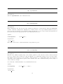
HMD for Computer Modeling
Alfred Paul Steffens-Jr
Copyright
Alfred Paul Steffens-Jr, 2002 – 2004
1
Table of Contents
Chapter 1: Downloading and Installing HMD
1
1. HMD Homepage
2. Required Libraries
1
1
Chapter 2: HMD as a Programmable Workspace
1. Starting the program
2. Interactive Command Prompt
3. Writing HMD Scripts
3
3
4
Chapter 3: Solving Differential Equations
7
1. The Equations of Mathematical Physics
2. Transformation to a Scalar Potential
3. Numerical Representation of the Second-Order PDE
Chapter 4: The Cell Grid Solver
1.
2.
3.
4.
5.
6.
7.
3
7
9
9
12
Introduction
Defining a Cell
Setting the Boundary Conditions
Growing a Cell Grid
Solving the Cell Grid
Manipulating the Cell Grid Solution Data
1-D Poisson’s Equation - Heat Transfer
12
12
14
15
16
17
19
Chapter 5: The Finite Element Solver
25
Chapter 6: Finite Element Examples
30
1.
2.
3.
4.
1-D
2-D
1-D
3-D
Electrostatics – Dielectric Layers
Electrostatics – Concentric Cylinders
Normal Modes – Stretched String
Normal Modes – Fluid Cylinder
31
37
46
54
i
Chapter 7: Command Reference
1.
2.
3.
4.
5.
6.
7.
8.
9.
10.
11.
12.
13.
14.
15.
16.
17.
18.
19.
20.
21.
22.
23.
24.
25.
26.
27.
28.
29.
30.
31.
32.
33.
34.
63
loadmesh
setregionbc
setregionbcn
setregiongrad
setregionmass
setregiondamp
setregionforce
buildglobalgrad
buildglobalmass
buildglobaldamp
buildglobalvector
setdivergence
seteigenmatrix
setsource
combinematrices
combinemodels
insertbcforce
insertbcmatrix
insertbcmodel
SOLVE
vec2file
solve div
solve eigen
setexpandelements
expandmatrix
exportmatrix
setbandpacked
createsparsity
set region force priorities
buildglobal invmatrix
buildglobal matrixproduct
impandmatrix
multiply by constant
convert to complex
63
63
64
66
66
67
67
68
68
69
69
70
70
71
72
72
73
73
74
74
74
75
75
77
77
78
78
78
79
80
81
81
82
82
Chapter 8: Utilities
84
1. INTP
2. DAT2VIS5D
3. WAVY
85
87
88
Chapter 9: Limitations and Future Development
1. Known Bugs
2. Mesh File Node Numbering
3. Cell Grid Shaping
89
89
89
89
ii
Chapter 1
Downloading and Installing HMD
§1. HMD Homepage.
HMD is freely available under the GNU public license. You may download the source code and user’s manual
from the HMD homepage at
http://www.heldeneng.com
Only the source code is available. The source code package is a standard GNU autotoolset package, which
means that you can easily build the software on your Unix-like operating system with the standard commands
./configure
make
make install
If you want to run HMD on Microsoft Windows, then you will need to install the Cygwin unix emulator. I
have used it. It installs like a charm and works great. After you have Cygwin on you windows machine you
can build HMD with the standard build commands listed above just as if you were running Unix.
§2. Required Libraries.
GNU Readline
HMD requires the READLINE package for the interactive console prompt. This package should be installed
on most Linux distributions, but I don’t know for sure which distributions have it. I know for sure that
Slackware comes with READLINE already installed. If your distribution doesn’t have it, then you need to
download it from the GNU site and build/install it on your machine. Or if you don’t want READLINE you
can build HMD without it but will not have an interactive prompt.
LAPACK
This is a well-known linear algebra package freely available at http://www.netlib.org/lapack
It was written and debugged by mathematicians E. Anderson, Z. Bai, C. Bischof, S. Blackford, J. Demmel,
J Dongarra, J. DuCroz, A. Greenbaum, S. Hammarling, A. McKenny, D. Sorensen. LAPACK is used in
Matlab, as well as other matrix algebra software programs such as Scilab and Octave and ALGAE. HMD
requires the LAPACK (Linear Algebra) library. You must go to the LAPACK webpage and download the
file lapack.tgz. It is free. But you must build it on your computer before you can build HMD. So, download
http://www.netlib.org/lapack/lapack.tgz
into the directory of your choice, say, /home/LAPACK. Now perform the following steps:
1. gzip -d lapack.tgz
1
2. tar xvf lapack.tar
The following build commands assume that you are using Linux. If you are using some other flavor of Unix
(or Cygwin on MS Windows) then consult the LAPACK documentation. At present I haven’t ported HMD
to any other platform (although this should all work on Cygwin).
3. cp make.inc make.inc.orig
4. cp install/make.inc.LINUX make.inc
5. make
Note: the make command is supposed to build and test everything. In my experience there will be a minor
problem with the BLAS library not being built. If this happens you can run the make command again in
the BLAS subdirectory. Check that you now have the two library files
lapack LINUX.a
blas LINUX.a
If the file blas LINUX.a is missing, then change directory to ./BLAS/SRC and run
make
again. Now you can move these two library files into a library directory of your choosing, let’s say LAPACKLIBS. You will need to remember this directory path and the names of the two libraries when you build
HMD.
GMSH
HMD is a model solver. So where are the neat wire-frame 3D images I wanted to see using a computer modeling tool? HMD uses another program for this. It’s called GMSH. It is available from www.geuz.org/gmsh
and can be downloaded for free. When used with HMD, GMSH is used as a standalone program, not a
library, so you don’t have to worry about building it. Just download it and install it.
You create a mesh file with GMSH. This file will have a file extension .msh. This file is what HMD needs to
complete its finite element model. The GMSH mesh file name is specified as an HMD script command.
GMSH is needed only when using the finite element solver. If you will be using the cellular grid solver only
then you will not need GMSH.
2
Chapter 2
HMD as a Programmable Workspace
§1. Starting the program.
HMD can be used as a batch processor or interactively. Batch mode is simply a matter of entering the script
file name at the command line:
hmd -f scriptfile
To run HMD interactively, just use the -i argument:
hmd -i
When you run HMD interactively you can still process script files with the source command. For example,
to execute the scriptfile mentioned above we would use
> source scriptfile ;
To exit the program, type exit.
§2. Interactive Command Prompt.
In interactive mode, HMD operates with a command line interface similar to Scilab and other software that
uses a workspace. The workspace has the capability to process commands, functions and variables. For
eample,
> x = 20;
> y = 10;
> z = x + y;
> msgprint z;
You must use a semicolon at the end of the statement. In some interactive languages like Matlab and Scilab,
if you leave off the semicolon the answer is automatically printed to the console. In HMD you must use the
msgprint command to see the result of a computation. All commands in HMD obey a simple syntax. The
command name is first followed by a list of comma-separared parameters:
> command name
paramater 1, paramater 2, ...
For example, you could use the msgprint command in the following way
3
> msgprint ’x + y = ’, z;
which would print x + y = 30 to the screen.
The interactive workspace environment gives you some convenience while working between commands. Its
pupose is mainly for storing and displaying variables and doing miscellaneous calculations. The operations
that can be performed in interactive mode are just a subset of those available in script processing mode.
§3. Writing HMD Scripts.
An HMD script is a list of source code to be executed. The HMD script language has many familiar features
to C programmers. You can declare variables, define functions, perform math operations, and perform
indirection. But these capabilities are meant only to support the main purpose of HMD, which is to solve
differential equations. The programmability features of HMD were not introduced so that you can write
whole applications in HMD as if it were another coding language like Fortran or C. With this in mind you
may be willing to forgive the HMD developers for not provided the full syntax support of the C language
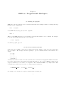
or the full matrix programmability of Scilab. Here is an example of an HMD script that does not solve any
differential equations, bit shows some of its programmability features.
//————————————————————————
// A Simple Programming Example
//————————————————————————
1
2
3
4
//
// Declare variables
//
double x;
double y;
double z;
//
// Initialize values
//
x = 2.0;
y = 3.0;
//
// Define a function
//
function multiply this { double a1, double a2 } {
double answer;
5
answer = a1 * a2;
6
7
}
8
//
// do processing
//
if ( x == 2.0 ) {
9
return answer;
z = multiply this( x, y );
4
10
msgprint z;
}
//————————————————————————
// End
//————————————————————————
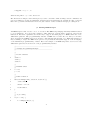
The first thing to note are the obvious differences from what you would expect from the C language:
Funtions
You use curly brackets instead of parenthesis for defining functions (but not calling them). You define a
function with the keyword function but without any type specifier. The first bracket that starts the function
definition must be on the same line with the function keyword (similar to tcl/tk). The closing bracket for
the function definition or conditional must be the first character on a line by itself.
Variable Declarations
At line 1 of the listing we see that variables were declared just like in the C language. The variable type
that can be declared include the following list
uchar
char
ushort
short
uint
int
ulong
long
float
double
complex
doublecomplex
However, if you don’t need special types and just want to do floating point math, then you can declare
variables on the fly (like in Scilab) which default to type double.
x = 2.0;
will automatically declare x in the workspace and make it a type double.
y = < 2.0 %i 7.0 >;
will automatically declare y in the workspace and make it a type doublecomplex.
Redirection
The HMD interpreter uses redirection similar to the C language. For conditionals you have if, else if, and
else. There is no switch statement. For looping you have while. There is no for statement or do-while
statement. The difference between the C language syntax and the syntax in HMD is that you must use curly
brackets to enclose the conditional code. In C, you can execute one following statement without using curly
5
brackets. But in HMD you must always use the curly brackets. Also, the first curly bracket must be on the
same line as the redirection identifier (I am not trying to enforce a particular coding standard, it was just
easier to write the parser this way).
6
Chapter 3
Solving Differential Equations
§1. The Equations of Mathematical Physics.
HMD was created especially for the purpose of solving a particular class of differential equations. These
have been referred to as the equations of mathematical physics because they arise so frequenty in the study
of physics. These differential equations are usually partial differential equations of the second order and
are the fundamental equtions in such disciplines as quantum mechanics, fluid mechanics, the mechanics of
continuum solids, acoustics, electromagnetic fields, and thermodynamics (heat transfer). Mathematicians
have classified these equations broadly into three types according to their time derivatives.
Elliptic
∂2ψ ∂2ψ ∂2ψ
+
+
=f
∂x2
∂y 2
∂z 2
(1)
∂2ψ ∂2ψ ∂2ψ
∂ψ
+
+
=f +α
2
2
2
∂x
∂y
∂z
∂t
(2)
∂2ψ ∂2ψ ∂2ψ
∂2ψ
+
+
=
f
+
α
∂x2
∂y 2
∂z 2
∂t2
(3)
Parabolic
Hyperbolic
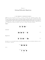
The sum of second-order partial derivatives is usually written in abbreviated form with the Laplacian operator
(in cartesian coordinates)
∇2 ≡
∂2ψ ∂2ψ ∂2ψ
+
+
∂x2
∂y 2
∂z 2
where
∂
∂
∂
∇ ≡ ~i
+ ~j
+ ~k
∂x
∂y
∂z
7
with which the following examples of partial differential equations in mathematical physics may be written
(see ”Mathematical Methods for Physicists”, 4th edition, Arfken and Weber, Academic Press, 1995)
Laplaces’s Equation
∇2 ψ = 0
(4)
This equation occurs in studies of
a.
b.
c.
d.
electrostatics, magnetostatics
hydrodynamics (irrotational flow of perfect fluid and surface waves)
heat flow
gravitation
Poisson’s Equation
∇2 ψ = −f
(5)
This is the nonhomogeneous analog of Laplace’s equation, being used where there are sources present.
Helmholtz Equation
∇2 ψ ± k 2 = 0
(6)
This equation can be found from the wave equation or diffusion equation by transforming its time dependence
into the fourier domain. This occurs in
a.
b.
c.
d.
elastic waves in solids including vibrating strings, bars, membranes
sound or acoustics
electromagnetic waves
nuclear reactors
Diffusion Equation
1 ∂ψ
a2 ∂t
∇2 ψ =
(7)
This equation is found in problems of heat transfer and gas dynamics.
Wave Equation
∇2 ψ =
1 ∂2ψ
a2 ∂t2
(8)
This equation is found in problems of wave propagation.
Nonhomogeneous Wave Equation
∇2 ψ =
1 ∂2ψ
−f
a2 ∂t2
8
(9)
This equation is found in problems of the radiation of electromagnetic waves, sound waves, etc.
The Schrödinger Equation
−
h̄2 2
∂ψ
∇ ψ + V ψ = ih̄
2m
∂t
(10)
which is, of course, the fundamental equation used in the quantum mechanics of atoms and elementary
particles.
§2. Transformation to a Scalar Potential.
It should be noted that the function ψ is a scalar and is, generally speaking, a potential field. When we
encounter differential equations involving vectors, for example, the electric field or a fluid velocity field, we
define a scalar potential such that
F~ = −∇ψ
(10)
from which the divergence operation encountered in the analysis of the vector field is transformed into a
second-order partial derivative of the scalar potential
∇ · F~ = −∇2 ψ
(11)
The use of a potential field representation is advantageous due to the well-developed theory that exists. The
essential features of the potential field is that it is continuous and its first-order derivative is continuous
except where there are sources. In ordinary language, this means that if you subdivide a region into smaller
regions, the potential values at the boundary of any subregion must match the boundary values of its nearest
neighbors. If a source exists in one of the subregions, then the first-order derivitive of the potential changes
at that point (the value of the source tells you by how much the derivative changes).
In addition to the continuity property, potential fields are local (a term from physics implying that action
induced by distant objects cannot happen). The value of the potential within a differentially small subregion
is the (weighted) average of the values at its boundaries, except if there are sources present. If there is a
source withing this subregion, then we must add a (weighted) contribution from it.
§3. Numerical Representation of the Second-Order PDE.
In the HMD solver the partial differential equations discussed above are represented by a general function
equation of the form
k(~x)∇2 ψ(~x) = F (t; ~x,
∂ψ
)
∂~x
(12)
This is a compact way of saying that the only thing that is really differenced is the Laplacian operator and
everything else in the equation is grouped on the right-hand side as part of F (t; ~x, ∂ψ
x)
∂~
x ). The multiplier k(~
is the weight assigned to the gradient at a particular point. In engineering this is often called a stiffness; in
electrostatics it corresponds to the dielectric constant or permitivity.
9
In equation 12 above the nonhomogeneous term, F , is shown as a function of the first derivatives of the
potential,
∂ψ
∂ψ ∂ψ
∂ψ
≡
,
,...
∂~x
∂x1 ∂x2
∂xn
The HMD solver is not designed for including the time derivatives in the function F . If the equation is
a time-dependent wave equation then the equation can be transformed into fourier space so that the time
derivative is replaced by a term −ω 2 ψ. The resulting Helmholtz equation would then be solved for normal
modes and frequencies. You should think of the HMD solver as capable of solving spacial problems. To time
step each spacial solution as with an ODE-type solver is not within the capabilities of the HMD solver. Or
you could experiment with treating time as a spatial dimension.
The core algorithm of the HMD solver suggests a grid composed of cells. Equation (12) is solved locally at
each cell and then its boundary values are matched to its nearest neighbors. Each cell has its own nodal
Green’s function solution that is solved based on its current (trial) boundary values. For linear problems the
Green’s function need only be calculated once. The solution is then comprised of the two-step interation of
updating the boundary values from the values of the nearest neighbors, then recalculating the local solution.
Recall from your undergraduate theoretical physics the Green’s function ”magic rule” solution of the Poisson
equation,
Z
ψ(~x) = −
ψ(~x0 )
s
∂G(~x, ~x0 ) 2 0
d x +
∂n0
Z
f (~x0 )G(~x, ~x0 )d3 x0 .
(13)
v
Those readers who are familiar with the green’s function solution of partial differential equations will note
that equation (13) is valid only for Dirichtlet boundary conditions. For those readers who have never seen
the green’s function solution, the function G(~x, ~x0 ) is the Green’s function. It is a propagator that produces
the effect of an impulse source at location ~x0 at the observation point at ~x. If there are no sources, then only
the surface integral is needed. If there are sources, then both integrals are needed. Note that the surface
integral is always required. Infinte boundary conditions as used in the ordinary finite element method will
need to be discussed later.
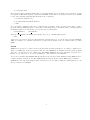
Now consider that we integrate Poisson’s equation in a infinitesimal volume. We first represent the equation
as a difference. To get an understanding of the derivation, first look at the one-dimensional case. Imagine
just three points with a value of the potential, ψ, assigned at each point, ψ1 = ψ(x1 ), ψ2 = ψ(x2 ), ψ3 =
ψ(x3 ). Between each point we may imagine an element of length δx with a weight of k(x). The numerical
representation can be written as follows.
h k (ψ − ψ) k (ψ − ψ ) ih 1 i
b
3
a
1
−
= f (x2 )
δx
δx
δx0
(14)
In equation (14) we denote the potential at x2 as ψ2 ≡ ψ because we wish to solve the potential at the
point x = x2 . The forcing function f (x) is evaluated only at x = x2 . The construction here implies that
we will solve for the value ψ at x2 given that we know the values of ψ at x1 and x3 and the value of f (x2 ).
Integrating equation (14) over δx0 results in the following equation.
kb (ψ3 − ψ) ka (ψ − ψ1 )
−
= f (x2 )δx0
δx
δx
Integrating equation (15) over δx results in
10
(15)
kb (ψ3 − ψ) − ka (ψ − ψ1 ) = f (x2 )δxδx0
(16)
and now solving for the potential ψ yields the local Green’s function solution.
ψ=
ka
δx
kb
ψ3 +
ψ1 − f
δx0
ka + kb
ka + kb
ka + kb
(17)
Equation (17) tells us that the value of the potential at x2 is the weighted sum of the values of its nearest
neighbors and adjusted for the effect of a change in slope at x2 .
In order to better see the resemblence to the Green’s function magic rule we can show the three-dimensional
equivalent of equation (17). If we write the numerical Laplacian with u1 , ψ, u3 along x, v1 , ψ, v3 along y, and
w1 , ψ, w3 along z, we have
qb (v3 − ψ) qa (ψ − v1 )
kb (u3 − ψ) ka (ψ − u1 )
rb (w3 − ψ) ra (ψ − w1 )
−
−
−
δy
δy
δx
δx
δz
δz
+
+
=f
δx0
δy 0
δz 0
(18)
Now integrate twice over the infinitesimal volume as above and solve for ψ. The solution is
δy 0 δz 0 δx0 δz 0 ψ = (ka u1 + kb u3 )
δyδz + (qa v1 + qb v3 )
δxδz
H
H
δx0 δy 0 δx0 δy 0 δz 0 +(ra w1 + rb w3 )
δxδy − f
δxδyδz
H
H
(19)
where
H = (ka + kb )δy 0 δz 0 δyδz + (qa + qb )δx0 δz 0 δxδz + (ra + rb )δx0 δy 0 δxδz.
(20)
Now compare equation (19) to equation (13). In the HMD algorithm, the factor δx0 δy 0 δz 0 /H is defined as
the numerical Green’s function valid locally at a node point. The HMD algorithm calculates equation (19)
at each node (refered to as a cell) and is defined as a deduce step. It will be seen that this calculation of ψ
at a node depends on the node values of the nearest neighbors. After a deduce operation is performed on
all the nodes the local boundary values, i.e., ka , kb , qa , qb , ra , rb , must be updated before the next iteration.
The operation of updating the local boundary values with the node values of the nearest neighbors is defined
as a link step in the HMD algorithm. Therefore, one complete iteration is a link step followed by a deduce
step. In other words, these two steps are repeated over and over until the desired accuracy in the model is
achieved.
11
Chapter 4
The Cell Grid Solver
§1. Introduction.
The cell grid solver is the primary solver algorithm in HMD. I began writing HMD as a finite element solver
(meaning the kind of finite element techniques familiar to structural engineers but with continuum elements),
but the limitations of the finite element technique soon became apparent. The cell grid solver works under
the premise of a grid as an array of cells. The idea of cellular automata in a rectangular array (inspired by
Stephen Wolfram’s book, A New Kind of Science) suggested cellular automata as a way of solving potential
theory problems. The cell rule is simply to match its boundary values with those of its nearest neighbors.
There is nothing surprisingly new about this, nor is this really a cellular automata algorithm.
The cell grid is different from the usual concept of a grid, but for the most part the user of this software
need not be alarmed. There are a few properties to remember when using the grid. A cell is primarily a
point in space, with its own potential value and its own Green’s function. It has connection points, two in
each dimension, that connect it to its neighbors. The connection points themselves are objects that provide
influence functions for the cell ”nucleus”, if you will, where the influence function may be used for a boundary
value (boundary value regarded as applying to the local cell only) or used as a weighted influence function
in the usual sense.
A single cell is first defined and given properties that will be inherited by the cells it ”grows” later to form a
grid. The first cell is defined with at least two steps. First the equation to be solved is defined; second, the
boundary conditions are set. The cell is then grown to fill an N-dimensional cube. Then the array of cells,
now forming a grid, is solved by repeatedly matching boundary values (link) and recalculating the potential
value (deduce). The iteration is stopped at an accuracy of the user’s choosing. The values of the grid may
then be copied into an array and saved to a file.
§2. Defining a Cell.
To define a cell takes two steps. The first step is to define the equation that will be solved. Recall equation
(12) in chapter 3.
k(~x)∇2 ψ(~x) = F (t; ~x,
∂ψ
)
∂~x
The cell grid algorithm understands this basic equation only. The first step in defining a cell is a command
that incorporates the information in the above equation with the exception of the weight, k(~x). The weight
information will be entered in the second step of the definition. Write the equation without the weight.
∇2 ψ(~x) = F (t; ~x,
12
∂ψ
)
∂~x
(1)
Now we enter a command that gives the cells name, ψ (”psi”), the Laplacian operator, the number of
dimensions, and the function F .
psi
Y:
<dimension>
∧
F
In the above pseudocode specification, Y: is equvalent to the Laplacian operator. Think of the wedge as like
the equal sign. We enclose the word ”dimension” in the <> symbols to designate that is is optional. If you
leave out the dimension specifier, then the dimension defaults to 1.
As an example that would be used in an HMD script, consider the one-dimensional Laplace’s equation.
∂2ψ
=0
∂x2
(2)
The cell definition command for this would be the following code line.
psi
:Y
1
∧
0 ;
If we use instead the two-dimensional Laplace’s equation,
∂2ψ ∂2ψ
+
=0
∂x2
∂y 2
(3)
then we would use the following HMD command.
psi
:Y
2
∧
0 ;
Or, consider a three-dimensional Poisson’s equation with a constant nonhomogeneous term.
∂2ψ ∂2ψ ∂2ψ
+
+
=7
∂x2
∂y 2
∂z 2
(4)
The HMD command line for this case would be the following code line.
psi
:Y
3
∧
7 ;
A Poisson’s equation with a general nonhomogeneous term that is a function of x, y, and z, becomes more
involved. Now we must define a function in the HMD workspace that will later be called by the HMD solver.
The Poisson’s equation of the form
∂2ψ ∂2ψ ∂2ψ
+
+
= F (x, y, x)
∂x2
∂y 2
∂z 2
will be specified in the HMD script with the following line.
13
(5)
psi
:Y
3
∧
My Function, 3, $1, $2, $3 ;
In the above command, ”My Function” is the name of user-defined function. The number 3 following the
function name specifies the number of arguments that follow. The first argument, $1, means the x coordinate
of the cell. Similarly, the second argument, $2, means the y coordinate of the cell, and $3 means the cell’s
z coordinate. It will be seen that the the user-defined function, ”My Function”, is a callback function. The
user writes this function to take three input arguments. The function assumes that it has been passed the
cell’s x, y, and z coordinates and returns its calculated value. The HMD solver algorithm will call this
function at each cell location. It knows what arguments that need to be passed to the function because these
were specified in the above cell definition.
It will be seen that the above code line is the general method for entering an equation resembling equations
(1) and (2). The callback function may take additional location-dependent arguments. To specify that the
cell’s grid spacing be passed to the function, one would use &1, &2, etc, instead of $1, $2, etc. To pass the
cell’s own value to the callback function (eigenvalue problem), one would write the argument as $0 name (
$0 psi in the above example ). Or to pass the first derivative (difference) of the cell’s value in x, y, or z, one
would give the argument as &1 psi, or &2 psi, or &3 psi.
§3. Setting the Boundary Conditions.
The boundary conditions for the cell should be set immediately after the cell definition, before any other
operations are attempted on the cell (such as growing the cell or starting the solution). The cell’s boundary
conditions as well as its weights are set with an anchor command. An anchor command is comprised of the
cell’s name followed by the anchor symbol, | (an underscore followed by a vertical line), followed by a list
of parameters that specify the boundary conditions and weights for each dimension as follows.
psi
|
bcx1 , wtx1 , bcx2 , wtx2 , bcy1 , wty1 , . . . ;
Think of the list of parameters as pairs of negative and positive terms for each dimension. For example, in
dimension 1 which is the x dimension, the negative and positive pairs correspond to left and right of the
cell. In dimension 2, which is the y dimension, the negative and positive pairs correspond to above and
below the cell. But the weights are also specified on the anchor line so there are 4, not 2 parameters for
each dimension. For example, for a one-dimensional cell with boundaries set to zero the following anchor
command would be used.
psi
|
0, 1, 0, 1 ;
The values of zero in the above command are setting the left and right boundaries to zero. The ones in the
above command are setting the weights on either side of the cell to one. Since the weight values are multiplied
with the boundary values, the above command corresponds to no weights. This would also coorespond to a
material with a stiffness (or permitivity) of unity.
When any one of the boundary value or weight value entries is required to be a function, then the single
entry becomes several entries that include the function name followed by the number of function arguments,
followed by the arguments themselves. For example, in the above simple, one- dimensional example let us
replace the zero boundary condition for the x dimension on the left with a function that takes two arguments.
14
psi
|
My Func, 2, myarg1, myarg2, 1, 0, 1 ;
Comparing the above anchor command with the previous example we see that where there was a single zero
specifying the left boundary value, now there are 4 entries: My Func, 2, myarg1, and myarg2. Then the
remaining anchor entries are as before. One might reflect that that is why the number of function arguments
must be specified: so that the parser knows where the logical argument ends and the next logical argument
begins.
Suppose now that we want the same function to provide the boundary values for both boundaries. Then the
anchor command would look like the following line.
psi
|
My Func, 2, myarg1, myarg2, 1, My Func, 2, myarg1, myarg2, 1 ;
We see in the above example that, again, what we previously had given as a single entry is now 4 entries.
Remember that there are still just four logical arguments, but that the 4 entries My Func, 2, myarg1, and
myarg2 form a single argument.
These boundary conditions are specified at the beginning of the setup procedure on a single cell. After the
cell is grown into a grid the boundary conditions will be applied only to the actual boundaries of the model.
As the grid is grown from a single cell each new cell that is reproduced carries with it the boundary value
information, but a boundary value is set only if the cell happens to be on the actual boundary.
Weight specifications, on the other hand, are applied everywhere in the model. In the above example, if the
values of one are replaced by some other constant, or variables, or function specifications, then these will be
the weights applied throughout the model.
The boundary values and the weights are calculated only once during the first iteration, by default. This
behavior can be changed so that either the boundary values or the weights or both are calculated on every
iteration with the initcell command.
§4. Growing a Cell Grid.
A cell grid is grown from a single cell one layer at a time. The grow command has a special operator in the
HMD solver. The grow operator is an arrow pointing to the right.
−>
For example, with a cell named ψ, the grow command would look the following line.
psi− >
To grow multiple layers we would either repeat this command on subsequent lines, or we could put it in a
while loop.
i = 0;
15
while (i < 10) {
psi − > ;
i = i +1 ;
}
Note that the grow operator’s component symbols, the dash followed by the > sign must not contain any
spaces between them.
§5. Solving the Cell Grid.
Now the cell (i.e., the seed of the grid) has been defined, and the boundary conditions set. The seed cell has
been grown into a grid. The process of solving the cell grid will cause the effect of the boundaries and the
sources to propagate throughout the grid. The grid gradually converges, that is, relaxes to its equilibrium.
This solution process requires iteration of two basic steps: link and deduce.
The link step has the effect of updating each cell member of the grid. Each cell has member objects that
contain the values of its local boundaries. In a link step the local boundary objects of a particular cell are
updated with the cell values of its nearest neighbors. For example, a one-dimensional cell will have two
boundary objects: one on the left and one on the right (negative x and positive x). During a link step this
cell’s left boundary object will be updated with the neighboring cell value to the left; the cell’s right-side
boundary object will be updated with the neighboring cell value on the right. The link step has the purpose
of completely isolating each cell when its potential value is deduced. The link step is merely an alternative
approach to maintaining a separate grid that would contain the previous or ”last” values that become inputs
to the ”next” iteration.
The link step has its own operator defined in the HMD solver: a greater-than sign and a less-than sign, ><.
A script command to link the cells in a grid whose seed cell was names psi would look like the following line.
>< psi ;
Note that the link operator comes before the cell name, not after it.
The second and final step in a solution iteration is a deduce step. The deduce step calculates an individual
cell’s potential value based on the values stored in its local boundary objects and the local value of the
forcing fucntion. The deduce step uses these values with the local Green’s function to calculate the cell’s
potential. The operator used for executing a deduce step is two question marks, ??. The command code for
executing a deduce step on the cell grid called psi is shown in the following line.
?? psi ;
Now to solve the cell grid names psi we must iterate the two steps, link and deduce, repeatedly until we
achieved the desired accuracy. This is shown in the following example.
i = 0;
while (i < 100) {
>< psi ;
?? psi ;
16
i = i +1 ;
}
In the above loop we are just guessing that 100 iterations would be sufficient for convergence. The HMD
solver has a built-in function for evaluating the accuracy of the solution. The function cellaccuracy scans
the group of cells and returns the least value of accuracy found in the group. This accuracy is calculated as
the absolute value of the difference between the cell’s value and its previous value divided by the previous
value. The above solution iteration loop can be re-written with the cellaccuracy function as follows.
double err;
err = 0;
while (err > 0.001) {
>< psi ;
?? psi ;
err = cellaccuracy(psi) ;
}
§6. Manipulating the Cell Grid Solution Data.
After the cell grid has been solved, the data (potential) contained at each cell can be extracted from the cell
group and placed into an array. This is done by extracting either a line or a plane. A line can be copied
into a one-dimensional array, and a plane can be copied into a two-dimensional array. The command that
obtains a line from the cell group is called getcell line. The command that obtains a plane from the cell
group is called getcell plane. In either case the command will create this new array for you and copy the
data into it. You may then save this data into an ascii data file for manipulation with other software tools.
The getcell line command is used with the following syntax.
getcell line < cell name > , < array name > , < coord flag >, < dim number >,
< location 1 >, < location 2 >, < i >, < j >, < k >, . . . ;
The arguments to the above getcell line command follow the following syntax:
<
<
<
<
<
<
<
cell name >
array name >
coord flag >
dim number >
location 1 >
location 2 >
i >, < j >, < k >,
the name of the cell (cell group)
the name of the array to be created
value of 1 means create a coordinate array also
which coordinate axis the line is parallel to
the start start index of the line
the end index of the line
...
a point on the line
It should be noted that the argument for < dim number > requires the numerical equivalent of ”x-axis”,
”y-axis”, etc, where x = 1, y = 2, z = 3, etc. The line to be extracted must be parallel to one of the
coordinate axes. The argument for < location 1 > is the location index of the cell where the line is to start.
17
Each cell has identifying indices (i = x, j = y, k = z, etc) for each dimension. Similarly, the argument for
< location 2 > is the location index of the cell where the line is to end. The last arguments comprise a list
of cell indices for a single cell somewhere on the line (you choose it). These indices uniquely identify the
location of the line to be extracted.
For example, consider a one-dimensional model from which you would like to extract the data. The getcell line
command in this case has only one line to copy from but which segment of the line is still to be determined
by your input parameters. Consider that the following model is a line in the x dimension whose cells have
indices numbered from -10 to +10. To extract the whole line into an array you would use the following
command.
int
ixdim, i1, i2;
ixdim = 1;
i1 = -10;
i2 = 10;
getcell line psi , ’vpsi’ , 1, ixdim, i1, i2, 0;
We see in the above example that the name of the cell group is psi. The name of the array to be created will
be called vpsi. The literal integer value of 1 that follows will cause a second array to be created containing
the coordinates (not the location indices) belonging to the cells. This is useful when plotting the data.
The second array will automatically have a name taken from the name of the primary array but with an s
appended. In this case the second array will be named vpsi s. The next argument, ixdim, has a value of
one and specifies that the x dimension is used. There is actually no other choice: the dimension number of
a one-dimensional model is automatically dimension number 1. The next two arguments, i1 and i2, specify
the endpoints of the segment to be extracted. Finally, the 0 value of the last argument specifies the cell
with location index 0 as the cell that uniquely identifies this line. In one dimension this last argument is, of
course, redundant. However, if you were to specify a location index in this last argument that is not within
the i1 and i2 endpoints you will get an error.
For example, consider a three-dimensional model from which you would like to extract a line for plotting.
This will be a line parallel to the z axis that intersects the x, y plane at the location indices 2, 3 in that
plane.
int
izdim, k1, k2;
izdim = 3;
k1 = -10;
k2 = 10;
getcell line psi , ’vpsi’ , 1, izdim, k1, k2, 2, 3, 0;
In the above example we can see that the dimension number is now 3, specifying a line parallel to the z
axis. The line endpoints are the same but now pertain to the z direction. There are now 3 indices, 2, 3, 0,
specifying a cell that uniquely identifies the line. This cell is located in the x, y plane and identifies the line
that passes through the point 2, 3. The position along the line is given as z = 0 but could have been any
other index between −10 and +10.
To extract a plane of data from a model the model must, of course, have at least two dimensions. The
getcell plane command has very similar syntax to the getcell line command but with extra parameters for
specifying the second dimension. Consider a two-dimensional model from which we would like to extract the
data.
18
int
ixdim, iydim, i1, i2, j1, j2;
ixdim = 1;
iydim = 2;
i1 = -10;
i2 = 10;
j1 = -10;
j2 = 10;
getcell plane psi , ’vpsi’ , 0, ixdim, iydim, i1, i2, j1, j2, 0, 0;
As with the getcell line command shown above, we see that the first arguments must be the name of the
cell group, psi, followed by the name to be given to the array, vpsi. In this example we will extract only
the cell potentials, not the cell coordinates also, so that the next argument is given as 0. The following two
arguments, ixdim and iydim specify the x, y plane. These arguments are redundant in this case because we
are extracting a plane from a model that is itself only a plane. The next two arguments, i1 and i2 give the
range in x, and the next two arguments, j1 and j2 give the y range. Finally, the last two arguments, 0 and
0, specify the location indices of a cell that uniquely identifies the plane to be extracted. But in this case
these two arguments are redundant since there is only one plane in the model.
After the data has been extracted from a cell group, you can save the data to a disk file. The save command
is used for saving one-dimensional arrays as columns in an ascii file. For example, the two one-dimension
arrays vpsi and vpsi s can be saved as a paired data set to a disk file called ”vpsi.dat” with the following
command.
save ’vpsi.dat’, vpsi s, vpsi;
The save2 command will save a two-dimension array (matrix) to a disk file. The following example shows
how to save the matrix called vpsi to a disk file called ”vpsi.dat”.
save2 ’vpsi.dat’, vpsi;
§7. 1-D Poisson’s Equation
-
Heat Transfer.
Consider Poisson’s equation for one dimension:
∂2ψ
= −f.
∂x2
(6)
The presence of the minus sign on the nonhomogeneous term is annoying but insures that the ”potential
change” is in the same direction as the ”force”. One should convince one’s self of the previous statement
by integrating equation (6) once over x and see that a positive force f δx0 acting at position x0 produces a
negative change in slope at x0 , which for zero Dirichtlet boundary conditions (the ends are pinned), must
result in a positive value of the potential at x0 .
To illustrate the one-dimensional Poisson’s equation we will examine the steady state heat transfer through
a thin bar. The bar is so thin that there is no variation in the y and z dimensions. The sides of the bar
are insulated so well that no heat is conducted through them, except at a single, small region where a heat
19
source is placed. The ends of the bar can conduct heat and are held at temperatures T1 and T2 . Let the
thermal conductivity, k, be uniform throughout the bar.
The differential equation to be solved for this problem is
k
∂2T
= −Q.
∂x2
(7)
where T is the temperature and Q is the heat source at x0 . First we should solve the problem with the
formulas of mathematical physics so that we can make a comparison with the numerical answer.
Problem 4-1. Show that the Green’s function for equation (7) is
x
L − x0
L − x0
+
2kL
2k
−x
L + x0
L + x0
+
2kL
2k
x < x0
x > x0
where x0 is the location of the unit impulse.
After you have learned how to solve differential equations you will find the theoretical solution to equation
(8) to be
Z
T (x) =
−L
xh
Z Lh L + x0 L + x0 i
L − x0 L − x0 i
0
0
−x
+
Q(x )dx +
x
+
Q(x0 )dx0 +
2kL
2k
2kL
2k
x
T − T T + T
2
1
2
1
x
+
2L
2
(8)
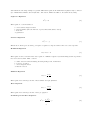
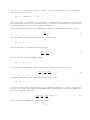
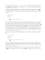
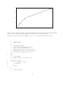
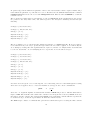
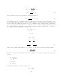
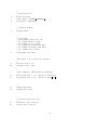
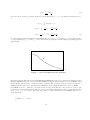
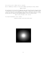
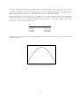
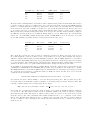
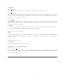
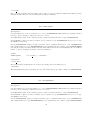
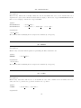
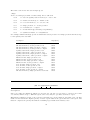
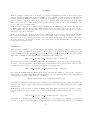
For this example we will assign a numerical value of 500 J/m3 · sec for the value of the source, Q(x0 ), and
let k have a value of 390 W/m · K. Let the distance, L, be 10 meters. The ends of the bar are held at
the constant temperatures T1 = 10 C, and T2 = 30 C. We will place the ”point” source at the location
x0 = −L/2 on the bar.
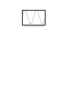
20
30
"temp1d_calc.dat"
25
20
15
10
-10
-5
0
5
10
The above figure shows the result for this problem when using equation (8) and plotted using GNUPLOT.
We will now solve this problem using the HMD cell grid solver and compare the results.
We will now set up a model script for HMD to solve the above temperature distribution problem.
1
2
//
// TEMP1D.HMD
//
//
// User’s manual example
// A 1D bar with a temperature distribution
// −L <= x <= L, L = 10 meters
// Temperature held at T 1 = 10C at the left end
// Temperature held at T 2 = 30C at the right end
// A ”point” source of 500 J/m3 ∗ sec at x = −5
//
int ic;
//
// a force callback
// impulse at location −L/2, where L = 10
//
function fc1 {double x} {
if (x > -5.01 && x < -4.99) {
return -500;
}
return 0;
3
4
5
6
7
}
//
//
//
declare a Divergence
21
8
9
10
11
12
13
14
15
16
17
18
19
20
21
22
23
24
25
26
//
// divergence with point force
// 1. Name of cell (to become a chain)
// 2. :Y means 2nd-order differential operator
// 3. / is the ”constraint” symbol (the right-hand side)
//
psi :Y ∧ fc1, 1, $1;
//
// set BC’s
// 1. Name of the cell
// 2. — is the ”anchor” symbol used for boundary conditions
// 3. List of BC / Stiffness values for each direction
//
The order is BC left, stiffness left, BC right, stiffness right
//
and repeated for each direction.
//
LEFT-HAND side
//
a. 10 C is the value at the left boundary
//
b. 390 is the value of all weights (in this case, thermal conductivity)
//
RIGHT-HAND side
//
c. 30 C is the value at the right boundary
//
d. 390 is the value of all weights (in this case, thermal conductivity)
//
psi | 10, 390, 30, 390;
//
//
//
// grow layers
//
ic = 0;
while (ic < 9) {
psi ->;
ic = ic+1;
}
//
// ”link cells”
//
>< psi;
//
// deduce the cell value
//
?? psi;
//
// solve
//
double errval;
ic = 0;
errval = 1.0e9;
while (errval > 0.0001 && ic < 1000) {
>< psi;
// link
?? psi;
// deduce
errval = cellaccuracy(psi);
ic = ic+1;
}
msgprint ’after link and deduce, ’, ic, ’ iterations’;
22
27
//
// extract the cell data as a plottable data set
//
// args:
// 1. Name of cell list
// 2. Name of array that will be created to hold the values
// 3. Flag that when nonzero creates the x-axis data
// 4. Dimension number (direction 1=x, 2=y, 3=z, etc)
// 5. Starting index for line data
// 6. Ending index for line data
// 7...N The list of direction indices specifying one point on the line
// Since this is 1-dimensional, there is only one index–we choose 0
//
getcell line psi, ’vpsi’, 1, 1, -9, 9, 0;
//
// save the data to a file
//
// args:
// 1. Name of output file to create
// 2...N The list of arrays (assumed to be 1 x N vectors) to form the
// columns of the data file
//
save ’vpsi.dat’, vpsi s, vpsi;
//
// print a 2-column data set fro the arrays
//
ic = 1;
while (ic <= 19) {
msgprint vpsi s[ic], ’ ’, vpsi[ic];
ic = ic + 1;
}
msgprint ’The End’;
28
29
30
31
32
33
34
Note the we make the sign of Q negative in the callback function f c1. The HMD green’s function is actually
not including the minus sign in equation (7), so we must put it into the solution. The function is defined at
line 2 and ”declared” on the cell creation line, line 8. The boundary values and the thermal conductivities
are assigned at line 9. The reader may be annoyed at the reference made in the above script to ”divergence”
do to the fact that the differential operator employed is actually the Laplacian.
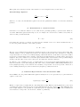
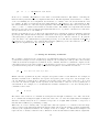
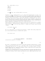
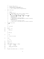
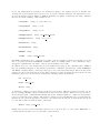
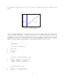
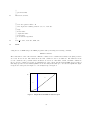
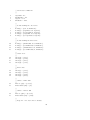
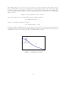
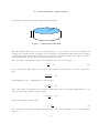
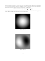
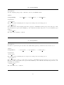
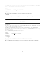
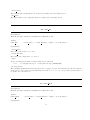
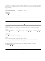
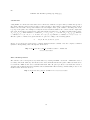
It should be emphasized that the HMD script above provides no display of the data result. The data is
saved to a disk file using the save command. In this case the output file will consist of two columns: the x
coordinates and the potential values. The resulting data are plotted with the GNUPLOT program in the
following figure. Comparing this figure with the previous figure obtained from the theoretical result we see
that the boundary values are missing in this plot. This is because the boundary values are not themselves
node values in the HMD algorithm.
23
30
’temp1d.dat’
28
26
24
22
20
18
16
14
12
10
-10
-8
-6
-4
-2
0
24
2
4
6
8
10
Chapter 5
The Finite Element Solver
If you already know how the finite element method works, then all you need to know is how HMD scripts
are set up. HMD reads an input script file containing the commands necessary for building and solving the
matrix equation for the model. HMD is run from the console command line with the following syntax:
hmd
-f
hmd script file
When you invoke HMD it is assumed that you have already built the mesh, and the mesh file name is given
as a parameter in the HMD script file. Alas, building the mesh is half of the job, and this is done with an
entirely separate program called GMSH. GMSH is written and distributed by Christophe Geuzaine and is
freely available for download at www.geuz.org. The output from GMSH will be a file with a .msh extension,
and this file is an input to HMD. In the examples included with HMD you will find files grouped in threes:
a .geo file, a .msh file, and a .hmd file. The .geo file is the input file for GMSH, and the result of running
GMSH is the .msh file. The .msh file and the .hmd file are both inputs for HMD. There is one important
caveat when building the GMSH .geo file: the physical region numbers must be renumbered from 1 to N
(see the examples).
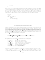
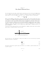
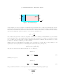
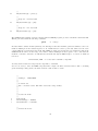
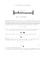
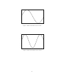
Consider the following simple physical problem as an illustration of HMD modeling. Take a stretched string
with a static force applied somewhere between its ends.
f
elasticity k
x=0
Fig. 1
x=a
x=L
Stretched string with applied force
We state without proof the mathematics of this problem, which is a second-order, inhomogeneous partial
differential equation in one dimension:
d2 u
=f
dx2
u(0) = 0
u(L) = 0
k
(1)
(2)
(3)
In the finite element method equation (1) is descretized into a set of difference equations assembled into one
big matrix equation:
Sb · ~u = f~
25
(4)
In equation (4), Sb is the numerical equivalent of the second-order derivative called a stiffness matrix, and f~
is the numerical equivalent of f called the force vector. We will create the stiffness matrix with the command
buildglobalgrad and create the vector with buildglobalvector. Then we will call SOLVE to obtain the
solution vector ~u.
The geometry is so simple that we can build the .geo file for GMSH without the graphical front end. Specify
two points for the ends, make a line, and define regions for the ends (the boundaries) and the line (the
material).
Point(1) = { 0.0, 0.0, 0.0, 0.1 };
Point(2) = { 10.0, 0.0, 0.0, 0.1 };
Line(1) = { 1, 2 };
Physical Point (1) = { 1 };
Physical Point (2) = { 2 };
Physical Line(3) = { 1 };
The above listing for a .geo file shows quite simply the structure of a GMSH input file. However, it will be
noticed that there is yet no way to specify the region where the force will be applied. So we will modify the
above listing by creating three line segments instead of just one, and the one ”Physical Line” statement will
become two statements: one for identifying the force region and one for the unforced region.
Point(1) = { 0.0, 0.0, 0.0, 0.1 };
Point(2) = { 3.0, 0.0, 0.0, 0.1 };
Point(3) = { 3.2, 0.0, 0.0, 0.1 };
Point(4) = { 10.0, 0.0, 0.0, 0.1 };
Line(1) = { 1, 2 };
Line(2) = { 2, 3 };
Line(3) = { 3, 4 };
Physical Point (1) = { 1 };
Physical Point (2) = { 4 };
Physical Line(3) = { 1, 3 };
Physical Line(4) = { 2 };
Now there are four regions: one for each endpoint, one for the string, and one for the small segment of string
where the force is applied. Now, to create the mesh file we can type at the console command line
gmsh
-1
geo file
where the ”-1” argument signifies one-dimensional elements. GMSH will produce a .msh file which will be
input to HMD. The mesh file will contain a list of all the nodes along the line created by GMSH, and below
that will be the list of all the line elements that GMSH created. Each line element will have specified the
nodes that belong to it and the region number in which the element resides.
The HMD script consists of commands that perform the well-known steps for creating the finite element
26
model. We assign physical constants to the elements belonging to the separate regions; we assemble the
elements into a global matrix and a global vector; we insert boundary values into the matrix and vector;
we solve the matrix equation. That’s it. HMD is essentially very simple. Consider the following commands
that are used in the building of this example model:
setregionbc
’string’, 1, ’polynomial’, 0.0 ;
setregiongrad
’string’, 3, 7.41 ;
setregionforce
’string’, 4, 2.73 ;
’string’, ’my stiffness matrix’ ;
buildglobalgrad
buildglobalvector
insertbcforce
’string’, ’force vector’ ;
string ;
insertbcmatrix
string ;
SOLVE
string ;
vec2file
’string’, ’string data.dat’ ;
The HMD commands are more or less just procedures, each one grouping together the steps that you would
have to program by hand in FORTRAN or Matlab. There is a similar format to the commands, being a
descriptive command name, the name of the model, an identifier, and a value.
In addition, there are a few details that are needed which merely support the command syntax. HMD is
like a programming language; it has variables, statements, commands, and functions. Unlike FORTRAN
and Matlab, variables must be declared by their type before being used–this is like C. The most important
variables are the model itself and the mesh. These variables are data structures that hold all the relevant
information needed to solve the model. Consider the following variable declarations:
int
my integer ;
mesh
model
string mesh ;
string ;
A declaration consists of a reserved keyword followed by the name it will have followed by a semicolon. In
the above listing, model is a keyword which defines string as a model variable. Then the word string will be
used in all subsequent commands that initialize this model. Always remember to define the mesh variable
before you define the model variable. The mesh is considered a more fundamental, more general structure
than the model. Several models may be attached to the same mesh. To this end, we must declare the model
not only with a name but with the name of the mesh.
model
string, ’string mesh’ ;
Finally, there is some top-level information that need to be given at the top of the script. HMD must be
told that this model will be solved by the finite element method.
27
string.modeltype =
FINITE ELEMENT ;
And the solver must know what kind of matrix equation is to be solved.
string.equation =
POISSON ;
The software distribution comes with a directory called ”examples” which includes example scripts. After
you look through a few of them you will see that they all follow the same steps.
To summarize, these are HMD modeling steps for following the finite element recipe.
1. Do some initial setup
Declare the mesh, give it a name, a type, and a file name.
Declare the model, give it a name, a type, and an equation.
2. Read the mesh file
loadmesh
3. Assign Boundary conditions
setregionbc
setregionbcn
4. Assign Material coeficients
setregiongrad sets the stiffness values
setregionmass sets the density values
setregionforce sets the force, charge, source term
5. Build the GlobaL Matrix and the Global Vector
buildglobalgrad builds the global stiffness matrix (associated with the gradient term)
buildglobalmass builds the global mass matrix (associated with the time derivative)
buildglobalvector builds the global forcing vector
6. Insert the Boundary Conditions into the Matrix and Vector
insertbcforce puts BCs into the global vector (must always be done first)
insertbcmatrix
7. Solve the Matrix Equation
SOLVE
8. Save the Answer to a File
vec2file saves the vector of nodal values to a file
28
gmvwrite saves the vector of nodal values to a GMV file
29
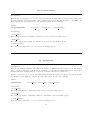
Chapter 6
Finite Element Examples
1. Poisson’s Equation
1-1.
1-D Electrostatics – Dielectric Layers
1-2.
2-D Electrostatics – Concentric Cylinders
2. Helmholtz Equation (wave equation)
2-1.
1-D Normal Modes – Stretched String
2-2.
3-D Normal Modes – Fluid Cylinder
30
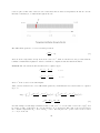
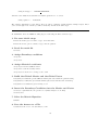
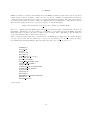
§1. 1-D Electrostatics – Dielectric Layers.
ε1
Φ1
ε2
Φ2
x
Figure 1. Two dielectric layers
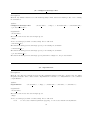
As an example, let us solve a simple one-dimensional problem that can be easily solved analytically as well.
Consider two dielectric layers that are bounded in the horizontal, the ~x, direction by thin, conducting plates.
The media extend without bound in the vertical direction. Because there will be no variation in the vertical
direction, the laplacian operator reduces to a second-order derivative in x
∇2 −→
d2 φ
dx2
We construct the problem so that the end plates are held at a constant potential difference by an external
battery and there are no fixed charges in the dielectrics. The potential at x = 0 will be V1 , and the potential
at x = L will be V2 . Let the position of the boundary between the two different dielectric media be xd . Our
problem is to find the potential, Vd , at this boundary.
~
Within each region, individually, the gradient of the potential is a contant. To see this, evaluate ∇ · D
separately in each region (that is, not including the dielectric interface). In region 1,
~ = 0 = ∇ · (o E
~ 1 + P~1 )
∇·D
and since the dielectrics are uniform, then ∇ · P~1 = 0. Therefore,
~1 = 0
∇·E
dφ1
V d − V1
= const =
dx
xd
(1)
similarly, for region 2,
~2 = 0
∇·E
dφ2
V 2 − Vd
= const =
dx
L − xd
The potential as a function of x in region one can be found by integrating equation (1).
dφ1 =
V d − V1
dx
xd
31
(2)
φ1
Z
dφ1 =
V1
φ1 (x) =
Vd − V 1
xd
Z
x
dx
0
Vd − V 1
x + V1
xd
(3)
The potential for region 2 can be found from integrating equation 2,
φ2 (x) =
V2 − V d
(x − xd ) + Vd
L − xd
(4)
The formulas for the two potentials in equations 3 and 4 depend on the value of the potential Vd . To solve
~ is a macroscopic field whose field
for Vd we will evaluate the equation ∇ · vecD = 0 at the interface, xd . D
~ which is discontinous
lines are defined as beginning and ending on free (not polarization) charge. Unlike E,
~
at the dielectric interface, D is defined to be continous across the boundary. A Gauss law pillbox enclosing
~ on each side of
the boundary interface in which the x dimension approaches zero yields the equality of D
the boundary. At the boundary interface, xd , we have
~1 −D
~ 2 ) · n̂ = 0
(D
D1 = D2
1 E1 = 2 E2
1
1
dφ2
dφ1
= 2
dx
dx
V d − V1
V2 − Vd
= 2
xd
L − xd
(5)
After doing the algebra and defining pa = 1 /xd and pb = 2 /(L − xd ) we can write the simple formula
Vd =
pa V 1 + pb V 2
pa + p b
(6)
We will choose the following physical values and enter them into these derived formulas, equations (3), (4),
and (6).
L = 0.6 meters
xd = 0.15 m
1 = 5.1
2 = 2.2
V1 = 1 volt
V2 = 10 volt
Inserting these values into equation (6) gives for Vd ,
Vd = 2.1314
32
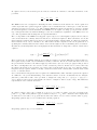
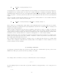
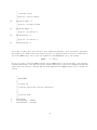
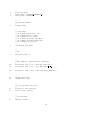
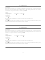
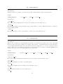
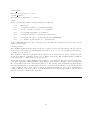
The formulas (3) and (4) can be used to plot the values of φ throughout the dielectric. This is shown in
figure 2.
Φ
10
9
8
7
6
5
region 1
region 2
4
3
2
x
1
0
0.1
0.2
0.3
0.4
0.5
0.6
Figure 2. Calculated potential
Now let us build an HMD model for the same problem and compare the results. This will be quit simple to
set up because this is essentially a one-dimensional model: there is no variation in the vertical direction. To
construct the mesh we merely need a straight line divided into two sections. The mesh file is created using
the GMSH program, written by Christophe Geuzaine, and freely available for download at www.geuz.org.
GMSH needs a geometry file as input, which we can build by using GMSH’s graphical inteface or by hand
with our text editor. The following small file took a few minutes with a text editor to create.
1
2
3
4
//
// FE22.GEO
//
// 1d model – 2 dielectric layers
//
scale = 0.02;
x0 = 0.0;
xd = 0.15;
L = 0.6;
5
6
7
//
// define the boundary and interface points
//
Point(1) = x0,0,0,scale; // left end-point
Point(2) = xd,0,0,scale; // interface
Point(3) = L,0,0,scale; // right end-point
8
9
//
// define lines that join them
//
Line(1) = 1,2; // dielectric region 1
Line(2) = 2,3; // dielectric region 2
33
//
// ”material” regions
//
// Region 1 – the left boundary
//
Physical Point(1) = 1;
//
// Region 2 – the right boundary
//
Physical Point(2) = 3;
//
// Region 3 – the dielectric 1
//
Physical Line(3) = 1;
//
// Region 4 – the dielectric 2
//
Physical Line(4) = 2;
10
11
12
13
Notice that we defined the point locations for the boundaries and interface , then created lines joining them,
then defined region numbers associated with each section. No material values are entered yet. That will be
done in the HMD script. Now to create the mesh file we run GMSH with our .geo file as input.
gmsh
-1
fe22.geo
Now we are ready to write the HMD script file. In the HMD script we specify the name of the mesh file,
fe22.msh, that should be read. We also specify boundary values (degree-of-freedom constraints) and material
values, such as the dielectric constants. The following listing shows the HMD script needed to calculate the
solution.
1
2
3
//
// FE22.HMD
//
//
// A 1-D model.
//
// 2 dielectric layers in the x direction, uniform in y
//
//
//
// declare the mesh
//
mesh tmesh;
tmesh.meshtype = GMSH;
tmesh.filename = ’fe22.msh’;
34
4
5
6
//
// Declare the model
//
model fe22, ’tmesh’;
fe22.modeltype = FINITE ELEMENT E;
fe22.equation = LAPLACE;
7
//
// read-in the mesh file
//
loadmesh tmesh;
8
//
// storage flags:
// bit 0: (0x01) sparsity table to file
// bit 1: (0x02) matrices to file(s)
// bit 2: (0x04) vectors to file(s)
// bit 3: (0x08) calc sparsity with cluster
// bit 4: (0x10) calc matrices with cluster
// bit 5: (0x20) double precision
//
createsparsity ’fe22’, 0x00;
9
10
//
// BC values — the potental of the end plates
//
setregionbc ’fe22’, 1, 1.0;
setregionbc ’fe22’, 2, 10.0;
11
12
//
// The ”stiffness” coefficients (electric permitivity)
//
setregiongrad ’fe22’, 3, 5.1; // dielectric 1, epsilon sub 1
setregiongrad ’fe22’, 4, 2.2; // dielectric 2, epsilon sub 2
13
14
//
buildglobalgrad fe22;
buildglobalvector fe22;
15
16
//
// set the type flag for the solver
//
setdivergence ’fe22’, ’fe22-grad’;
setsource ’fe22’, ’fe22-force’;
35
17
//
// put in the BCs
//
insertbcmodel fe22;
18
//
// solve the equation A*X = B
// and output the resulting solution vector to ’fe22.dat’
//
// args:
// model name
// output file name
// solver flags
// node-selection specifiers
//
solve div ’fe22’, ’fe22.dat’, 0x00, ’all’;
19
EXIT;
Using the above HMD script, the HMD program is run by invoking the following command,
hmd -f fe22.hmd
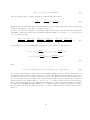
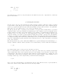
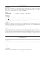
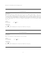
The result will be a file called fe22.dat. This file consists of five columns and as many rows (lines) as there
are nodes in the model. The numbers in the first column are the node numbers. The numbers in the
second column are the potential values calculated at each node. The third, fourth, and fifth columns are
the x,y, and z coordinates at each node. Examination of the output data shows that HMD gives a result for
this single-precision model indistinguishable from the analytical result up to at least four significant digits.
Compare the data plotted in figure 3 to the analytical plot in figure 2.
10
Φ
9
ε2
8
7
6
ε1
5
4
3
2
1
0
0.1
0.2
0.3
0.4
0.5
0.6
x
Figure 3. Output data from HMD for dielectric layers
36
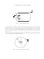
§2. 2-D Electrostatics – Concentric Cylinders.
y
z
x
φo = 0
φ
Rb
Ra
ρ
εa
εb
φo = 0
Figure 1. Concentric dielectric cylinders
Consider an infinitely long cylinder containing a cylindrical charge distribution. The outer shell has radius
Rb and is held at a electric potential φo . This could be accomplished if the shell were made of a conducting
material, but we will ignore the conductivity for this problem. Let the charge distribution extend to a radius
Ra and be denored by ρ. The region included within Ra has a dielectric permitivity of a . The region
Ra < r < Rb will have a permitivity of b . We wish to find the electric potential, φ, everywhere within the
cylinder r < Rb .
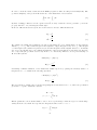
Because there is no variation along the axial direction of the cylinder, say the z direction, the derivitives
in z are zero. The divergence and laplacian operators reduce to 2-D operators, and so we may take a cross
section of the cylinder and treat this as a 2-D problem.
φo
r
Rb
εa
ρ
Ra
φ (r)
Figure 2.
εb
2-D cross section of concentric cylinders
37
In order to check the result obtained from the HMD program we will solve this problem analytically. The
geometric simplicity of the problem allows the use of the Gauss Law of electrostatics:
I
~ · dS
~=
D
Z
ρdV
S
(1)
V
~ we may obtain the electric potential, φ, from the
By first obtaining a function for the electric field, E,
~
~
property that E = −∇φ and integrate E through r.
In the two different dielectric regions, the electric field becomes two different functions:
~
~a = D
E
a
~
~b = D
E
b
(2)
(3)
~ over a virtual surface at the arbitrary
We evaluate the Gauss Law formula in region B by integrating D
distance ra < r < rb . The volume integral on the right side of (1) is integrated only out to ra . The integral
over the length of the cylinder is represented by L, and the integration in the angular direction, θ, is trivially
2πr. we see as well that due to the cylindrical symmetry of the problem that the electric field can only have
an r component (the potential does not vary in the θ or z directions). Therefore, we drop the subscript on
Er and call it just E.
b Eb L(2πr) = ρL(πra 2 )
Eb (r) =
ρra 2
2b r
(4)
Performing a similar evaluation of the Gauss Law within region A, by placing the arbitrary surface of
integration at r < ra results in the following expression:
a Ea L(2πr) = ρL(πr2 )
Ea (r) =
ρr
2a
(5)
The electrostatic potential can be found by integrating the electric field from r = rb , where the potential is
grounded, to a point r within the cylinder.
~ = −∇φ
E
Z 2
~ · d~l
φ2 − φ1 = − E
1
This is equivalent to the work that must be done to move a point charge toward the region of central charge
density from the outer shell. For region B, the integration will be from r = rb to r.
Z
φb (r) = −
rb
38
r
Eb (r)dr
φb (r) =
ρra 2
rb
ln( )
2b
r
(6)
For region A, we add the potential obtained by integrating from rb to ra to the functional integral from ra
to r.
r
Z
φa (r) = −
Ea (r)dr + φba
ra
r
Z
φa (r) = −
ra
φa (r) =
ρra 2
rb
ρ
rdr +
ln( )
2a
2b
ra
rb
ρ
ρra 2
(ra 2 − r2 ) +
ln( )
4a
2b
ra
(7)
Choosing physical values that will scale well numerically, we choose a = 5.1 (glass), b = 2.2 (polypropylene),
ρ = 10 (coulombs/m3 ), ra = 0.1m, rb = 0.5m. The Scilab plot in figure 3 shows equations (6) and (7) plotted
again radius.
0.05
0.04
φ
0.03
0.02
0.01
0
0
0.1
0.2
0.3
0.4
0.5
r
Figure 3. Plot of calculated electric potential
We will now model this 2-D problem using HMD and GMSH. The grid of x,y points and elements is created
using the GMSH (www.geuz.org) program. The HMD modeling program is designed to read a GMSH output
file (mesh file) and use that to construct its finite elements. The geometry of the problem is entered into a
GMSH input file, called a .geo file. From this GMSH produces a mesh file that will be used by HMD.
For GMSH we need to define two concentric circles and (1) tell it that the outer circle is a ”region” (the
boundary), (2) tell it that the inner disk is a ”region” (the charge distribution), and (3) tell it the the outer
area, ra < r < rb , is a ”region” (the dielectric). The code given in listing 1 is the GMSH script used to
create the mesh.
//
// listing 1.
//
fe19.geo
39
// 2-D model for Mach II
//
1
2
3
4
bigradius= 0.5;
smallradius = 0.1;
bigscale = 0.1;
smallscale = 0.02;
5
6
7
8
9
//
// Points defining the outer circle
//
Point(1) = {0, 0, 0, smallscale};
Point(2) = {bigradius, 0, 0, bigscale};
Point(3) = {0, bigradius, 0, bigscale};
Point(4) = {-bigradius, 0, 0, bigscale};
Point(5) = {0, -bigradius, 0, bigscale};
10
11
12
13
//
// Points defining the inner circle
//
Point(6) = {smallradius, 0, 0, smallscale};
Point(7) = {0, smallradius, 0, smallscale};
Point(8) = {-smallradius, 0, 0, smallscale};
Point(9) = {0, -smallradius, 0, smallscale};
14
15
15
17
//
// Outer circle
//
Circle(1) = {2,1,3};
Circle(2) = {3,1,4};
Circle(3) = {4,1,5};
Circle(4) = {5,1,2};
18
19
20
21
//
// Inner circle
//
Circle(5) = {6,1,7};
Circle(6) = {7,1,8};
Circle(7) = {8,1,9};
Circle(8) = {9,1,6};
22
23
//
// surface of inner disk
//
Line Loop(9) = {5,6,7,8};
Plane Surface(10) = {9};
24
25
//
// surface of Outer disk
//
Line Loop(11) = {1,2,3,4};
Plane Surface(12) = {11,9};
//
// Region 1 – the outer circle boundary
40
26
//
Physical Line(1) = {4,1,2,3};
27
//
// Region 2 – the inner disk
//
Physical Surface(2) = {10};
28
//
// Region 3 – the outer disk
//
Physical Surface(3) = {12};
The GMSH script is listing 1, when compiled with the GMSH program, produces a mesh file called fe19.msh.
This is performed with the following command:
gmsh
-2
fe19.geo
Because this model has circular symmetry, I would suspect that the mesh file generated will have some node
numbers missing from the natural sequence 1..N. I think this is because a point was defined for the circle
centers which is not included in the mesh. The HMD program expects that the node numbers found in the
GMSH mesh file will be in the range 1..N, with no indices missing from the sequence. To be sure that the
mesh file conforms to this rule, we will filter the mesh file through an AWK script to reorder node numbers
if needed:
cat fe19.msh | awk -f reorder.awk fe19.msh > tmp.msh
You may then rename the temporary file, tmp.msh, to fe19.msh.
Now we are ready to write the HMD script that will compute the finite element solution. The code listing
given in Listing 2 will generate the finite element solution that we desire.
1
2
3
//
// Listing 2, FE19.HMD
//
//
// A 2-D model.
// Two concentric circles. The inner circle has a chage density.
//
//
//
//
// declare the mesh
//
mesh tmesh;
tmesh.meshtype = GMSH;
tmesh.filename = ’fe19.msh’;
//
// Declare the model
41
4
5
6
//
model fe19, ’tmesh’;
fe19.modeltype = FINITE ELEMENT E;
fe19.equation = POISSON;
7
//
// read-in the mesh file
//
loadmesh tmesh;
8
//
// storage flags:
// bit 0: (0x01) sparsity table to file
// bit 1: (0x02) matrices to file(s)
// bit 2: (0x04) vectors to file(s)
// bit 3: (0x08) calc sparsity with cluster
// bit 4: (0x10) calc matrices with cluster
// bit 5: (0x20) double precision
//
createsparsity ’fe19’, 0x00;
9
//
// BC
//
setregionbc ’fe19’, 1, 0;
10
11
//
// The ”stiffness” coefficients (electric permitivity)
//
setregiongrad ’fe19’, 2, 5.1; // inner disk, epsilon sub a
setregiongrad ’fe19’, 3, 2.2; // outer disk, epsilon sub b
12
setregionforce ’fe19’, 2, 10.0; // inner disk, charge distribution
13
14
//
buildglobalgrad fe19;
buildglobalvector fe19;
15
16
//
// set the type flag for the solver
//
setdivergence ’fe19’, ’fe19-grad’;
setsource ’fe19’, ’fe19-force’;
17
//
// put in the BCs
//
insertbcmodel fe19;
42
18
//
// solve the equation A*X = B
// and output the resulting solution vector to ’sol.dat’
//
// args:
// model name
// output file name
// solver flags
// node-selection specifiers
//
solve div ’fe19’, ’sol.dat’, 0x00, ’all’;
19
EXIT;
The HMD script above can be explained in terms of the basic steps required for assembling a finite element
model. Lines 1 through 6 are variable declarations, namely of the Mesh structure and the Model structure.
The mesh declarations cause HMD to allocate and initialize a structure to hold the mesh coordinates and
node identifier numbers. The model structure is a top-level object that allows access to all the parameters
that apply to this particular model.
The GMSH program will have created a file called fe19.msh which contains all the coordinates and node
numbers (and material region numbers). This information is loaded into HMD on line 7 of the script. Line
8 creates a special structure for holding the sparsity information of the model. Consequently, the matrices
produced for the model will be stored internally in a packed format (packed matrices are specified by model
type FINITE ELEMENT E, while unpacked matrices are specified by FINITE ELEMENT).
On lines 9 through 12 we enter the material coefficients. To the engineer, these are the material properties
and degree-of-freedom (DOF) constrains. To the mathematician, these are the linear coefficients on the
differential equation and the boundary values.
Lines 13 and 14 comprise the primary usefulness of HMD. These commands take the mesh information and
the material coefficients and construct a matrix for each ”element” in the mesh and assemble all the element
matrices into one global matrix and one global vector. The idea is that we will solve the matrix equation
Sb · ~u = f~
(8)
b and buildglobalvector creates the vector f~. Lines
The command buildglobalgrad constructs the matrix S,
15 and 16 are important only within the contect of the HMD programming langauge. During the model
construction the matrices and vectors and given ”types”, which are essentially states in the process. Here we
set the stiffness matrix to have a type DIVERGENCE and the forcing vector to have a type SOURCE. This
is like changing to solution mode. (lines 15 and 16 are required for a model of type FINITE ELEMENT E,
but not FINITE ELEMENT). Line 17 modifies the global matrix and global vector to contain the contraints
or boundary values (which were specified on line 9).
At this point, you may export the constructed matrix and vector to ascii files and use some other software
to solve the matrix equation, say Matlab or Scilab or Algae. You would do that with
expandmatrix ’fe19’, ’fe19-grad’, ’gradfile.dat’;
and
expandvector ’fe19’, ’fe19-force’, ’forcefile.dat’;
However, HMD has the capability to solve the matrix equation, and this is what is specified on line 18. This
command will result in a file called sol.dat which contains the solution. The solution is the value calculated
at each node position. The structure of the output file is 5 ascii columns with as many lines as there are
nodes in the model. Column 1 is the node number; column 2 is the nodel value (the answer); column 3, 4,
43
and 5 are the x,y, and z coordinates of the node on that line.
The above HMD script, fe19.hmd, is executed with the HMD program using the following command:
hmd -f fe19.hmd
The output file is sol.dat, as specified in the HMD script. The output data is in the form of the electric scalar
potential evaluated at each of the node points, which is difficult to examine visually. The HMD program
comes with an interpolation program, INTP, that creates a matrix of regularly-spaced values. For example,
an image of the data may be created using INTP by making a matrix of raw, binary pixels, then converting
that raw image into a displayable image (using ImageMagick or your favorite image program):
intp -d sol.dat -g fe19.msh -b scalar -o fe19.raw
Now, using the ImageMagick ”convert” command,
convert -size 417x417 -depth 8 gray:fe19.raw fe19.pdf
44
The resulting image above looks more like a long exposure of a star from an astronomical camera, but the
larger potential values are shown as the brighter pixels, and the smaller values are the darker pixels. With
your favorite image program you may create a false-color image that better identifies the potential distribution. If you would rather use Matlab or Scilab to display the interpolated values, there is a corresponding
INTP command,
intp -d sol.dat -g fe19.msh -a scalar -o fe19.mat
Now the file fe19.mat can be read into Matlab with the dlmread command:
M = dlmread (’fe19.mat’, ’ ’);
And the cooresponding command for Scilab is
M = read (’fe19.mat’, -1, 417);
Now that we have the Matlab-able file of data values, we can extract a profile line from the matrix and
compare this result to the theoretical calculation displayed in figure 3. From the matrix, M, that was read
into Matlab, a profile can be taken at row 208 and columns 208 through 417.
0.05
Theoretical (black)
0.04
0.03
Φ
Numerical (blue)
0.02
0.01
0
0
0.1
0.2
0.3
0.4
Figure 5. Comparison of results
45
0.5
§3. 1-D Normal Modes – Stretched String.
displacement
Φ
x=L
x=0
Figure 1. Stretched String
On a string stretched between two points, x = 0 and x = L, a wave travels to the right, f+ (x − vt). The
endpoints are fixed so that the wave is reflected as f− (x + vt). The combination of the forward and reflected
waves results in a standing wave, F (x, t). This standing wave of arbitrary shape may be represented as the
superposition of normal modes. A normal mode by definition has the property that every material element
moves (vibrates) with the same phase, so the position and time coordinates are independent. This motivates
the separation of variables x and t so that each normal mode function is a product of two functions
Fω (x, t) = φω (x)Tω (t)
.
The form of φω (x) is found by the solution by separation of variables of the wave equation in the region
x = 0 to x = L. Without reproducing the derivation, we may state that when the wave equation
1 ∂2φ
∂2φ
=
∂x2
c2 ∂t2
is separated into equations for x and t, the equation in x is the homogeneous Helmholtz equation
∂2φ
+ k2 φ = 0
∂x2
(1)
where k = ω/c.
The solution to differential equation (1) is sin(kx). The wave number , k, is found by fitting the solution to
the boundary coinditions. At x = L the mode function sin(kx) must be zero so that
kL = nπ
or
k=
nπ
L
(2)
where n takes on all the integer value from 1 to ∞.
Notice that equation (1) is an eigenvalue equation whose eigenvalues are k 2 . Since HMD has an eigenmode
solver, we should be able generate the vibrational modes of this string with HMD and compare the result
46
with the known answer. Let the length, L, of the string be 1 meter, and let the sound speed, c, in the material
be 200 meters per second. Then the modal frequencies given by equation (2) are given in the following table
(in hertz):
n
f
1
2
3
4
100
200
300
400
This is a rather simple model to construct in HMD. The mesh is trivial in that you merely have to draw
a line with GMSH and specify the endpoints as separate regions. The following code listing is the GMSH
input file used to produce the simple stretched string mesh.
//
// FE7.GEO
//
// A stretched string (1-d FE problem)
//
1
2
//
// end points
//
Point(1) = 0, 0, 0, 0.01;
Point(2) = 1, 0, 0, 0.01;
3
//
// the line
//
Line (1) = 1, 2;
4
//
// Region 1 – the line
//
Physical Line (1) = 1;
5
//
// LHS point
//
Physical Point (2) = 1;
6
//
// RHS point
//
Physical Point (3) = 2;
47
The above input file must now be compiled by the GMSH program to produce the mesh file. Since the input
file is called fe7.geo, the mesh file will be automatically named by GMSH to be fe7.msh. This mesh file will
be an input file to HMD.
gmsh
-1
fe7.geo
Notice that we use a -1 as an argument to GMSH. This specifies that the mesh will be one-dimensional. If
you were to create the GEO file using the GMSH graphical interface then you would merely press the F1
key to generate a mesh (or the F2 key for a two-dimensional model, or the F3 key for a three-dimensional
model).
Now we need an HMD input file. The following code listing is an HMD script that will create the finite
element matrix equation for the string normal modes and solve it.
1
2
3
//
// FE7.HMD
//
// Solve Eigen Modes equation
// 1-D
// A line in the x-direction, represents a stretched string
//
//
//
//
// declare the mesh first
//
mesh tmesh;
tmesh.meshtype = GMSH;
tmesh.filename = ’fe7.msh’;
4
5
6
//
// Declare the model
//
model tmodel, ’tmesh’;
tmodel.modeltype = FINITE ELEMENT;
tmodel.equation = EIGENMODES; // means d2̂U/dx2̂ + k2̂ U = 0
7
//
// read-in the mesh file
//
loadmesh tmesh;
//
// set physical values for each region, each model
//
48
8
9
// —————————————————————–
// BC
// Region 2 – the LHS boundary point
// Pinning the LHS point, setting the node value to zero.
//
setregionbc ’tmodel’, 2, ’polynomial’, 0.0; // perimeter
//
// BC
// Region 3 – the RHS boundary point
// Pinning the RHS point, setting the node value to zero.
//
//
setregionbc ’tmodel’, 3, ’polynomial’, 0.0; // perimeter
// —————————————————————–
11
//
// Region 1 – the string itself
//
//
// GRAD
// The ”grad” coefficient is the stiffness
// But here, we normalize the equation so that the ”mass” coeficient
// contains all the physics
//
setregiongrad ’tmodel’, 1, 1.0;
//
// MASS
// The ”mass” coefficient is 1 / c2̂, i.e., reciprocal of sound-speed
// squared
//
// Le the length of the string be 1 meter
// Let the frequency (fundamental) be 100 Hz
// The sound speed = 2 * L * f
// c = 200 m/s
// 1 / c2̂ = 2.5e-5
//
setregionmass ’tmodel’, 1, 2.5e-5;
12
13
//
// build the global Gradient matrix
//
buildglobalgrad ’tmodel’, ’grad’;
buildglobalmass ’tmodel’, ’mass’;
10
//
//
//
//
//
//
apply boundary conditions
this function applied BC’s to the Grad and Mass
matrices separately–because the LAPACK routine
for solving it will take them separately, not combined.
49
14
//
insertbceigen tmodel;
15
//
// solve the FE matrix
//
SOLVE tmodel;
16
17
//
// output the eigenvalues
//
eigenvalueswrite ’tmodel’, ’fe7-vals.dat’;
//
// output the eigenvectors (each column is a vector)
//
eigenvectorswrite ’tmodel’, ’fe7-vecs.dat’;
//
// (the node indices corresponding to each row in these files
// will be automatically saved in ”tmodel-packlist.dat”
//
// end
It should be pointed out that there are a few code statements in this file that seem inconsistent with
the other code listings that were presented. Notice that the model type is FINITE ELEMENT not FINITE ELEMENT E as was used in previous examples. This tells you that the above script is using HMD’s
original, primitive algorithm that I call ”mach I”. Although this algorithm is no longer under development,
it works, and I don’t plan to remove it as it serves as a check when doing diagnostics. Other differences are
that there is no createsparsity statement; the setregionbc statement has a ”polynomial” specifier that is not
needed in the updated algorithm; the updated algorithm always uses insertbcmodel whereas here we have
insertbceigen; the updated algorithm specifies the output file name in the solve eigen command whereas here
we have the SOLVE command followed by two separate commands for writing output files for the eigenvectors and eigenvalues. This ”mach I” algorithm has only limited capability: it has only single precision; you
can’t choose which LAPACK solver routine to use with a bit-field flag as in the updated algorithm.
We will now solve the model by issuing the following command at the command prompt:
hmd -f fe7.hmd
The output file generated are
fe7-vals.dat
fe7-vecs.dat
tmodel-packlist.dat
The first two files contain the eigenvalues and eigenvectors, respectively. The third file is produced only when
50
using the old, mach I algorithm. It contains a list of node numbers that are the cross reference into the file
of eigenvectors. When boundary values are set to zero, the corresponding node positions are removed from
the global matrix since these rows and columns would merely produce unit eigenvectors. We keep track of
which node positions correspond to components in the eigenvector with the packlist.
The eigenvalues file, fe7-vals.dat, is easy to decipher as it is a single column ascii file. The eigenvalues
contained in this file are the angular frequency squared. To convert to frequency in hertz you must take
the square root and divide by 2π. The following table shows the first few eigenvalues and the corresponding
frequencies obtained from the HMD model.
ω2
f
394859.0
1580040.0
3556280.0
6325540.0
100.009476
200.057194
300.136010
400.284649
The first four mode shapes that are output from HMD are shown in figures 2 through 5. We recognize the
familiar sin function.
320
280
240
200
160
120
80
40
0
0
0.1
0.2
0.3
0.4
0.5
0.6
0.7
0.8
0.9
Figure 2. Mode 1 from column 1 of fe7-vecs.dat
51
1.0
300
200
100
0
-100
-200
-300
0
0.1
0.2
0.3
0.4
0.5
0.6
0.7
0.8
0.9
1.0
Figure 3. Mode 2 from column 2 of fe7-vecs.dat
300
200
100
0
-100
-200
-300
0
0.1
0.2
0.3
0.4
0.5
0.6
0.7
0.8
0.9
Figure 4. Mode 3 from column 3 of fe7-vecs.dat
52
1.0
300
200
100
0
-100
-200
-300
0
0.1
0.2
0.3
0.4
0.5
0.6
0.7
0.8
0.9
Figure 5. Mode 4 from column 4 of fe7-vecs.dat
53
1.0
§4. 3-D Normal Modes – Fluid Cylinder.
Consider the resonant modes inside a cylinder filled with fluid.
R
h
Figure 1. Cylinder filled with fluid.
The scalar variable will be the velocity potential defined by ~v = −∇φ. We then solve for the normal modes
of this scalar potential. For the calculation of mode frequencies it is immaterial that this scalar potential is
an artificial quantity. But for the specification of the boundary conditions we must discover how φ is related
to the pressure, since pressure the wave equation variable for a fluid.
The conservation of momentum equation for a fluid (just Newton’s Second Law) is
ρ
∂~v
= −∇p
∂t
(1)
where ρ is the static fluid density and p is the acoustic pressure. Substituting ~v = −∇φ into equation (1)
gives
ρ
∂(−∇φ)
= −∇p
∂t
interchanging the order of differentiation on the left gives
−ρ∇(
∂φ
) = −∇p
∂t
Since ρ is a zeroth-order quantity, it is considered constant with respect to the spacial differentiation. So we
may put it inside the gradient operation giving
−∇(ρ
∂φ
) = −∇p
∂t
and now integrating both sides gives
p=ρ
∂φ
∂t
(2)
The normal mode problem is actually in frequency space, as we are solving the homogeneous Helmholtz
equation
54
∇2 φ + k 2 φ = 0
(3)
The φ in equation (3) is therefore φ(~r, ω), so the time derivative in equation (2) is transformed to frequency
space by
∂φ
= −jωφ
∂t
(4)
Then substituting equation (4) into equation (2) we obtain the relation between the acoustic pressure and
the scalar potential,
p = −jρωφ
(5)
Therefore, when we set homogeneous dirichtlet boundary conditions we are really setting the pressure to
zero, and when we set homogeneous Neumann boundary conditions we are setting the fluid velocity to zero.
The normal mode frequencies are found analytically by solving equation (3) in cylindrical polar coordinates.
The procedure is to substitute the ∇2 operator with its cylindrical coordinate equivalent operator, then
perform separation of variables. The following result was taken from Arfken, Mathematical Methods for
Physicists, 2nd edition, page 635.
φ = Σmnk Jm (
αmn
r)e±jmθ (amn sin(kz) or bmn cos(kz))
a
(6)
The index m identifies the dimetral mode, the index n identifies the radial mode, and the index k corresponds
to modes in the z direction. When r = a we want the radial mode shape, Jm to be zero. So the αmn are
the zeros of Jm given by
n
J0 (x)
J1 (x)
J2 (x)
J3 (x)
1
2
3
2.4048
5.5201
8.6537
3.8317
7.0156
10.1735
5.1356
8.4172
11.6198
6.3802
9.7610
13.0152
At z = 0 and z = h we want φ to vanish, so in equation (6) we choose the axial mode shape to be sin(kz).
This boundary condition forces the values of k to be
k=
pπ
h
where p = 0, 1, . . .. For homogeneous, dirichtlet boundary conditions, the mode frequencies are given by (see
Arfken)
r
ωmnp = c
αmn 2
p2 π 2
+
a2
h2
(7)
where c is the sound speed.
Let the sound speed be set to c = 200m/s, the radiua a = 12m, and the height h = 6m. We can use
equation (7) and table (1) to calculate what the first few frequencies should be. The magnitudes of the
Bessel zeros in table (1) will govern the order in which the eigenvalues will be found. The values of the index
p in equation (7) will start at 1, not zero. This is because we are pinning the boundary value to zero at
55
z = 0 and z = L: therefore there can be no pure translation mode in the z direction. The first frequency
(in radians) is ω011 = 112.128, the second will be ω111 = 122.656, the third will be ω211 = 135.250, and the
fourth is ω021 = 139.393.
Now let us use HMD to solve this problem and compare its answer with the theoretical solution. Building a
cylinder in GMSH is a simple matter. The following GEO file is the input to the GMSH program that will
produce the necessary MSH file:
//
// fe23.geo
//
// Cylinder, 3D
//
1
2
3
4
scale = 1.7;
radius = 12;
z1 = 0;
z2 = 6;
5
6
7
8
9
//
// bottom disk
//
Point(1) = 0, 0, z1, scale; // center
Point(2) = radius, 0, z1, scale;
Point(3) = 0, radius, z1, scale;
Point(4) = -radius, 0, z1, scale;
Point(5) = 0, -radius, z1, scale;
10
11
12
13
14
//
// top disk
//
Point(6) = 0, 0, z2, scale; // center
Point(7) = radius, 0, z2, scale;
Point(8) = 0, radius, z2, scale;
Point(9) = -radius, 0, z2, scale;
Point(10) = 0, -radius, z2, scale;
15
16
17
18
//
// arcs for bottom disk
//
Circle(1) = 2,1,3 Plane0,0,1;
Circle(2) = 3,1,4 Plane0,0,1;
Circle(3) = 4,1,5 Plane0,0,1;
Circle(4) = 5,1,2 Plane0,0,1;
//
// arcs for top disk
//
56
19
20
21
22
Circle(5)
Circle(6)
Circle(7)
Circle(8)
=
=
=
=
7,6,8 Plane0,0,1;
8,6,9 Plane0,0,1;
9,6,10 Plane0,0,1;
10,6,7 Plane0,0,1;
23
24
25
26
Line(9) = 5,10;
Line(10) = 2,7;
Line(11) = 3,8;
Line(12) = 4,9;
27
28
29
30
31
32
33
34
//
// surface around the rim
//
Line Loop(13) = 10,-8,-9,4;
Ruled Surface(14) = 13;
Line Loop(15) = 11,-5,-10,1;
Ruled Surface(16) = 15;
Line Loop(17) = 12,-6,-11,2;
Ruled Surface(18) = 17;
Line Loop(19) = 9,-7,-12,3;
Ruled Surface(20) = 19;
39
40
//
// top and bottom surface
//
Line Loop(21) = 8,5,6,7;
Plane Surface(22) = 21;
Line Loop(23) = 4,1,2,3;
Plane Surface(24) = 23;
//
// the volume
//
Surface Loop(26) = 22,14,16,18,20,24;
Volume(27) = 26;
41
//
// Region 1 – the rim
//
Physical Surface(1) = 14,16,18,20;
42
//
// Region 2 – top and bottom
//
Physical Surface(2) = 22,24;
35
36
37
38
//
57
// region 3 – the volume
//
Physical Volume(3) = 27;
43
To create the MSH file we must run GMSH, specifying the above file as its input. The following command
will run GMSH and create the MSH file:
gmsh
-3
fe23.geo
Now we create the HMD script file. The following script file tells HMD to use the MSH file we just created
and generate the finite element solution.
1
2
3
//
// FE23.HMD
//
// Solve Eigen Modes equation
// 3-D
// A cylinder
//
//
//
//
// declare the mesh first
//
mesh tmesh;
tmesh.meshtype = GMSH;
tmesh.filename = ’fe23.msh’;
4
5
6
//
// Declare the model
//
model tmodel, ’tmesh’;
tmodel.modeltype = FINITE ELEMENT E;
tmodel.equation = EIGENMODES;
7
//
// read-in the mesh file
//
loadmesh tmesh;
8
//
// set physical values for each region, each model
//
createsparsity ’tmodel’, 0x00;
58
9
10
// —————————————————————–
// BC
// Region 1
// Pinning the boundary, setting the node values to zero.
//
setregionbc ’tmodel’, 1, 0.0; // perimeter
setregionbc ’tmodel’, 2, 0.0; // top and bottom
// —————————————————————–
12
//
// Region 3 – the cavity itself
//
//
// GRAD
// The ”grad” coefficient is the stiffness
// But here, we normalize the equation so that the ”mass” coeficient
// contains all the physics
//
setregiongrad ’tmodel’, 3, 1.0;
//
// MASS
// The ”mass” coefficient is 1 / c2 , i.e., reciprocal of sound-speed
// squared
//
setregionmass ’tmodel’, 3, 2.5e-5;
13
14
//
// build the global Gradient matrix
//
buildglobalgrad ’tmodel’, ’grad’;
buildglobalmass ’tmodel’, ’mass’;
15
16
setdivergence ’tmodel’, ’grad’;
seteigenmatrix ’tmodel’, ’mass’;
17
//
// apply boundary conditions
//
// this function applied BC’s to the Grad and Mass
// matrices separately–because the LAPACK routine
// for solving it will take them separately, not combined.
//
insertbcmodel tmodel;
11
//
// solve the FE matrix
//
// flags:
59
18
// bits 0-3: 0= use LAPACK, symmetric, generalized eigenvalue solver
// bit 4: 1= use symmetric-packed solver (use upper triamgle)
// bit 5: 1= use SPARSPAK band-packing of sparse matrix
// bit 7: 1= don’t calculate eigenvectors
//
solve eigen ’tmodel’, ’fe23.dat’, 0x10, ’all’;
19
//
// (the node indices corresponding to each row in these files
// will be automatically saved in ”tmodel-packlist.dat”
//
EXIT;
// end
In the above script listing for FE23.HMD, notice the bit flags argument to the solver in line 18. Here we use
bit 4, which in hexidecimal is 0x10. This flag specifies that we will use a symmetric-packed solver and so (in
principal) reduce the memory requirements. This algorithm works on global matrices that are symmetric,
which will usually be the case for a simple finite element problem with no damping. Since the matrices are
symmetric, we only need the upper triangle, thereby reducing the memory requirements by half. However,
in the above script the memory requirements have not really been reduced because all the eigenvectors have
been requested. The solver must allocate a full N x N matrix to hold the eigenvectors. Had we desired
to calculate a solution with the eigenvalues only and no eigenvectors, we would have set bit 7 in the flags
argument. The hexidecimal representation of the flags would then have been 0x90.
The memory requirements could have been reduced still further had we set bit 5 instead of bit 4. This
algorithm actually rearranges the global matrices to put all the nonzero matrix elements near the diagonal
so that a very efficient packing can be accomplished. If you try this you will find extra ones in the list of
eigenvalues. These are part of the unit vector space that results when homogenous boundary values are
given. The other algorithms remove the unit vector space by default, making the output easier to read.
To run the above script, type the following command at the system command prompt:
hmd -f fe23.hmd
The output data are written to the file fe23.dat. The first column in this file is comprised of the node
numbers. Unlike the Poisson solver, the node numbers here are not important in relation to the eigenvalues.
This is because the LAPACK eigenvalue equation solver outputs the eigenvalues in increasing order, which
is not necessarily the same order as the node numbers. However, the node numbers do in fact correspond
to the vector component locations so that the eigenvector components can be assigned to the appropriate
spacial locations when doing graphics on them.
The second column in the file contains the eigenvalues. These values are equivalent to ω 2 . In order to obtain
the frequency in hertz you must take the square root and divide by 2π. Columns 3 through 5 are the x,
y, and z coordinates belonging to each node number in column 1. Starting in column 6 the mode vectors
(eigenvectors) are listed. Column 6 is mode 1, column 7 is mode 2, etc.
Comparing the output from HMD with the theoretical result calculated above we obtain the following table
of values (as ω):
60
eigenvalue (ω)
Theoretical
HMD output
deviation (%)
ω011
ω111
ω211
ω021
112.128
122.656
135.250
139.393
116.450
128.69
143.118
147.986
3.9
4.9
6.3
6.2
We used a mesh containing 1002 nodes, which for a three-dimensional model is somewhat small. The accuracy
(or lack of accuracy) of the above results is due to the coarseness of the mesh. If you use the GMSH graphical
interface to examine this mesh you will notice that in the z direction there are something like 3 to 4 elements
in the z direction. As a rule of thumb, we should try to get at least 10 elements in any direction if we need
good accuracy. However, a model with a larger mesh will take much longer to execute on the computer.
This problem was recalculated using a finer mesh. You can reproduce the finer mesh by making a change in
the GEO file. At line (1) in the above GEO file listing change 1.7 to 0.9. This will produce a mesh having
5973 nodes. On a 900 Mhz pentium III PC with 512 Mb of RAM HMD took about 2 hours to solve this
model. The resulting eigenvalues and the accuracy is shown in the table below.
eigenvalue (ω)
Theoretical
HMD output
deviation (%)
ω011
ω111
ω211
ω021
112.128
122.656
135.250
139.393
113.349
124.282
137.434
141.810
1.1
1.3
1.6
1.7
The output file, fe23.dat, is so large because it contains the eigenvectors. Each component of the vector is
the scalar magnitude of the mode shape at the corresponding node location. Three-dimensional output is
difficult to display without using powerful visualization software. But the HMD distribution comes with a
utility program called INTP (interpolation program) which can scan the output file through a chosen plane
to produce an image, like a CAT scan slice through the three-dimensional figure. With a simple model such
as this we should be able to recognize radial and dimetral mode shapes in the interpolated slice.
To use INTP we need an input file with 5 columns. This is exactly the output format obtained when we run
a POISSON or LAPLACE model with HMD. But the result of the eigenvalue model contains N + 5 columns.
The HMD distribution comes with an AWK script, mode2datII.awk, for extracting a given eigenvector from
the output file and producing a 5-column file usable by INTP. To extract the first mode vector from the
output file use the following command:
cat fe23.msh | awk -f mode2datII.awk md=fe23.dat mdn=1 > mode1.dat
Now with mode1.dat we will use INTP to create the interpolated image slice. The program can produce
its output either as an ASCII file readable by Matlab or as a binary image in raw (no header) format. The
following command will produce a binary image file as output.
intp -d mode1.dat -g fe23.msh -b scalar -o fe23 1.raw -s -12, -12, 3, 12, -12, 3, 0, 12, 3
Notice that the -b argument specifies the output as binary. If you want an ASCII file instead, substitute
a -a for the -b. The slice plane is defined by the -s argument. Think of the plane as defined by a square
sheet that slices the figure. The square is defined by three points: two at its bottom corners and one at the
midpoint of the top line. The -s argument takes 9 numbers which are the x, y, z coordinates of each of these
three points. The first three numbers are the coordinates of the lower-left point. The second three numbers
are the coordinates of the lower-right point, and the last three numbers are the coordinates of the upper,
midsection point.
61
This program takes a long time to execute, as it is not a very efficient algorithm. When the program finishes
we can convert the raw image format into a JPEG file or whatever other image format you like using Image
Magick. The following command converts the raw image into a JPEG image.
convert -size 417x417 -depth 8 gray:fe23 1.raw fe23 1.jpg
Here is what the lowest mode shape, sliced through a plane bisecting the z axis, looks like in a 256 gray-level
image. The model with 5973 nodes was used to produce this result.
Figure 2. Mode 1
Figure 3. Mode 2
62
Chapter 7
Command Reference
§1. loadmesh.
description
Loads a mesh file previously set as the filename member of ”mesh”. The mesh variable name is the only
argument, bcause the file name has already been set before this command is called. The mesh variable must
have been declared before this command.
syntax
loadmesh
<mesh name>;
arguments
<mesh name>
The variable name identifying the mesh. This is not a string, so don’t enclose it in quotes.
§2. setregionbc.
description
Sets the desired dirichtlet boundary condition for the specified region.
syntax −− (mach I)
setregionbc
<model name> <region number> <function type> <constant> [(<axis> <order>
<coefficient>), . . . ] ;
syntax −− (mach II)
setregionbc
<model name> <region number> <value or function name>
arguments
<model name>
The variable name identifying the model given as a string enclosed in single quotes.
63
<region number>
The region number. The boundary value will be applied to all nodes grouped into this region. The region
numbers are given in the GMSH .geo and .msh files and must range from 1 to the maximum region number.
arguments −− (mach I only)
<function type>
This is either ”polynomial” or ”rational” (in single quotes). The reason this is here is because the boundary
value is ideally a function of x, y, and z. To set the boundary value to a constant, you just provide the
zeroth-order term of a polynomial.
<constant>
The boundary value. This is actually the zeroth-order term of a polynomial, but if the boundary value is to
be set as a constant this value will be the last parameter on the line.
optional mach I arguments
<axis>
If the boundary value is to be a polynomial function of x, y, and z, then this parameter identifies which
direction. For x, x2 , x3 , . . . the parameter would be ”x” (in single quotes). For any power of y the parameter
would be ”y”, and so on.
<order>
The power of either x, y, or z.
<coefficient>
The polynomial coefficient of the term in x, y, or z.
arguments −− (mach II only)
<value or function name>
Set a constant real value, or the name of a previously-defined function. If a function name, then it must
have an underscore prefix. When you define this function, think of it like a callback function that expects
to have 3 arguments passed to it: x, y, and z.
§3. setregionbcn.
description
Sets the desired neumann boundary condition for the specified region.
syntax −− (mach I)
setregionbcn
< model name>, < region number>, < function type>, < constant>, [(< axis>, <
order>, < coefficient>), . . . ] ;
syntax −− (mach II)
setregionbcn
<model name> <region number> <value or function name>
64
arguments
<model name>
The variable name identifying the model given as a string enclosed in single quotes.
<region number>
The region number. The boundary value will be applied to all nodes grouped into this region. The region
numbers are given in the GMSH .geo and .msh files and must range from 1 to the maximum region number.
arguments −− (mach I only)
<function type>
This is either ”polynomial” or ”rational” (in single quotes). The reason this is here is because the boundary
value is ideally a function of x, y, and z. To set the boundary value to a constant, you just provide the
zeroth-order term of a polynomial.
<constant>
The boundary value. This is actually the zeroth-order term of a polynomial, but if the boundary value is to
be set as a constant this value will be the last parameter on the line.
optional mach I arguments
<axis>
If the boundary value is to be a polynomial function of x, y, and z, then this parameter identifies which
direction. For x, x2 , x3 , . . . the parameter would be ”x” (in single quotes). For any power of y the parameter
would be ”y”, and so on.
<order>
The power of either x, y, or z.
<coefficient>
The polynomial coefficient of the term in x, y, or z.
arguments −− (mach II only)
<value or function name>
Set a constant real value, or the name of a previously-defined function. If a function name, then it must
have an underscore prefix. When you define this function, think of it like a callback function that expects
to have 3 arguments passed to it: x, y, and z.
65
§4. setregiongrad.
description
Sets the stiffness coefficient for the model’s GRAD (stiffness) matrix.
syntax
setregiongrad
< model name>, < region number>, < constant value> ;
arguments
<model name>
The variable name identifying the model given as a string enclosed in single quotes.
<region number>
The region number. The stiffness value will be applied to all GRAD elements grouped into this region. The
region numbers are given in the GMSH .geo and .msh files and must range from 1 to the maximum region
number.
<constant value>
The value of the stiffness coefficient.
§5. setregionmass.
description
Sets the mass (inertial) coefficient for the model’s MASS matrix.
syntax
setregionmass
< model name>, < region number>, < constant value> ;
arguments
<model name>
The variable name identifying the model given as a string enclosed in single quotes.
<region number>
The region number. The mass value will be applied to all MASS elements grouped into this region. The
region numbers are given in the GMSH .geo and .msh files and must range from 1 to the maximum region
number.
<constant value>
The value of the inertial coefficient.
66
§6. setregiondamp.
description
Sets the damping (energy loss) coefficient for the model’s DAMP matrix.
syntax
setregiondamp
< model name>, < region number>, < constant value> ;
arguments
<model name>
The variable name identifying the model given as a string enclosed in single quotes.
<region number>
The region number. The damping value will be applied to all DAMP elements grouped into this region. The
region numbers are given in the GMSH .geo and .msh files and must range from 1 to the maximum region
number.
<constant value>
The value of the damping coefficient.
§7. setregionforce.
description
Sets the force (non-homogeneous term of the differential equation) coefficient for the model’s vector.
syntax
setregionforce
< model name>, < region number>, < constant value> ;
arguments
<model name>
The variable name identifying the model given as a string enclosed in single quotes.
<region number>
The region number. The force value will be applied to all FORCE elements (element vectors) grouped into
this region. The region numbers are given in the GMSH .geo and .msh files and must range from 1 to the
maximum region number.
<constant value>
The value of the force coefficient.
67
§8. buildglobalgrad.
description
This command performs the act of combining the individual element matrices into one global model matrix.
In this case, the element matrices will be stiffness matrices. The resulting matrix will become a member
data structure to the given model and be of matrix type GRAD.
syntax
buildglobalgrad
< model name>, < matrix ID> ;
arguments
<model name>
The variable name identifying the model given as a string enclosed in single quotes.
<matrix ID>
The matrix ID is a string enclosed in single quotes. Here you are providing an identifier with which you may
uniquely identify this matrix in the subsequent modeling commands.
§9. buildglobalmass.
description
This command performs the act of combining the individual element matrices into one global model matrix.
In this case, the element matrices will be mass matrices. The resulting matrix will become a member data
structure to the given model and be of matrix type MASS.
syntax
buildglobalmass
< model name>, < matrix ID> ;
arguments
<model name>
The variable name identifying the model given as a string enclosed in single quotes.
<matrix ID>
The matrix ID is a string enclosed in single quotes. Here you are providing an identifier with which you may
uniquely identify this matrix in the subsequent modeling commands.
68
§10. buildglobaldamp.
description
This command performs the act of combining the individual element matrices into one global model matrix.
In this case, the element matrices will be damping matrices. The resulting matrix will become a member
data structure to the given model and be of matrix type DAMP.
syntax
buildglobaldamp
< model name>, < matrix ID>, < detID or flags > ;
arguments
<model name>
The variable name identifying the model given as a string enclosed in single quotes.
<matrix ID>
The matrix ID is a string enclosed in single quotes. Here you are providing an identifier with which you may
uniquely identify this matrix in the subsequent modeling commands.
< detID >
This optional 3rd argument gives the ID string of a determinant struct (the object that is built by createsparsity), that already exists, from which this matrix will derive its properties. If no 3rd argument is given,
then the first determinant struct belonging to the model is used (the sparsity map created by the first call
to createsparsity or when the first model matrix was built).
or
< flags >
If the optional 3rd argument is an integer instead of d̈etID,̈ then this is understood to be a set of bit-coded
flags having the same meanings as the flags given to the createsparsity command. If flags are given to this
command, then a new determinant struct (sparsity map) is created just as if the createsparsity command
were being called. If no 3rd argument is given, then the first determinant struct belonging to the model is
used (the sparsity map created by the first call to createsparsity or when the first model matrix was built).
§11. buildglobalvector.
description
This command performs the act of combining the individual element vectors into one global model vector.
The resulting vector will become a member data structure to the given model and be of vector type FORCE.
syntax
buildglobalforce
< model name>, < vector ID> ;
arguments
<model name>
The variable name identifying the model given as a string enclosed in single quotes.
69
<vector ID>
The vector ID is a string enclosed in single quotes. Here you are providing an identifier with which you may
uniquely identify this vector in the subsequent modeling commands.
§12. setdivergence.
description
Sets the matrix type for a model matrix to be of type DIVERGENCE. This matrix type designates that it
is ready to have boundary conditions set and to be solved.
For LAPLACE’s equation, the matrix going into solution activities should be of type DIVERGENCE.
For POISSON’s equation, solution activities expect a matrix of type DIVERGENCE and a vector of type
SOURCE (see setsource).
For the EIGENMODE equation, solution activities expect a stiffness matrix set to type DIVERGENCE
and a mass matrix set to type EIGENMATRIX (see seteigenmatrix). If no matrix of type EIGENMATRIX
is found the solution activities assume that the mass matrix was inverted and multiplied into the stiffness
matrix, so that a ”standard eigenvalue” problem is assumed.
syntax
setdivergence
< model name>, < matrixID>;
arguments
<model name>
The variable name identifying the model given as a string enclosed in single quotes.
<matrixID>
The matrix ID string (enclosed in single quotes) of the matrix whose type will be changed to DIVERGENCE.
§13. seteigenmatrix.
description
Sets the matrix type for a model matrix to be of type EIGENMATRIX. This matrix type designates that it
is ready to have boundary conditions set and to be solved.
For LAPLACE’s equation, the matrix going into solution activities should be of type DIVERGENCE.
For POISSON’s equation, solution activities expect a matrix of type DIVERGENCE and a vector of type
SOURCE (see setsource).
For the EIGENMODE equation, solution activities expect a stiffness matrix set to type DIVERGENCE
and a mass matrix set to type EIGENMATRIX (see seteigenmatrix). If no matrix of type EIGENMATRIX
70
is found the solution activities assume that the mass matrix was inverted and multiplied into the stiffness
matrix, so that a ”standard eigenvalue” problem is assumed.
syntax
seteigenmatrix
< model name>, < matrixID>;
arguments
<model name>
The variable name identifying the model given as a string enclosed in single quotes.
<matrixID>
The matrix ID string (enclosed in single quotes) of the matrix whose type will be changed to EIGENMATRIX.
§14. setsource.
description
Sets the vector type for a model vector to be of type SOURCE. This vector type designates that it is ready
to have boundary conditions set and to be solved.
For LAPLACE’s equation, the matrix going into solution activities should be of type DIVERGENCE.
For POISSON’s equation, solution activities expect a matrix of type DIVERGENCE and a vector of type
SOURCE (see setsource).
For the EIGENMODE equation, all vectors are ignored.
syntax
setsource
< model name>, < vectorID>;
arguments
<model name>
The variable name identifying the model given as a string enclosed in single quotes.
<vectorID>
The vector ID string (enclosed in single quotes) of the vector whose type will be changed to SOURCE.
71
§15. combinematrices.
description
Adds two matrices belonging to the same model. The resulting matrix replaces the first matrix.
syntax
combinematrices
< model name>, < matrix 1>, < matrix 2> ;
arguments
<model name>
The variable name identifying the model given as a string enclosed in single quotes.
<matrix 1>
The matrix ID string (enclosed in single quotes) of first matrix to combine. This matrix will be overwritten
by the resulting matrix.
<matrix 2>
The matrix ID string of the second matrix to combine (enclosed in single quotes).
§16. combinemodels.
description
Mach I only. Combines several individual models into one supermodel in which each of the component
matrices form blocks in the resulting block matrix. The sequence of arguments lists the models and their
corresponding matrix ID strings as block positions, from left to right and top to bottom order, in the block
matrix. After the block dimension is specified, the arguments follow in triplets of model, matrix, and
vector, until every block in the final matrix has been provided.
syntax
combinemodels
< supermodel name>, < block dim>, < model 1>, < mID 1>, < vID 1>, . . . ;
arguments
<supermodel name>
The variable name identifying the final model given as a string enclosed in single quotes.
<block dim>
The matrix dimension, in blocks, of the final matrix.
<model 1>
The first model name given as a string enclosed in single quotes.
<mID 1>
The first matrix ID string enclosed in single quotes.
<vID 1>
72
The first vector ID string enclosed in single quotes.
§17. insertbcforce.
description
Mach I only. Inserts the boundary values into the model vector. This command must be called before
the corresponding command for the model matrix. This is because for dirichtlet boundary conditions the
boundary value must be first multiplied on each matrix value in the corresponding column and added to the
vector. The process of inserting dirichtlet boundary values into the matrix involves setting the corresponding
row and column values to zero, so the vector boundary operations must be done before the matrix column
is set to zero.
syntax
insertbcforce
< model name> ;
arguments
<model name>
The variable name identifying the model given as a variable (not in quotes).
§18. insertbcmatrix.
description
Mach I only. Inserts the boundary values into the model matrix.
syntax
insertbcmatrix
< model name> ;
arguments
<model name>
The variable name identifying the model given as a variable (not in quotes).
73
§19. insertbcmodel.
description
Mach II only. Inserts the boundary values into the model matrix and vector. If no matrix and vector
arguments are given, then it finds the first matrix belonging to this model of type DIVERGENCE and the
first vector belonging to this model of type SOURCE.
syntax
insertbcmodel
< model name> ;
insertbcmodel
< model name>, < matrix ID>, < vector ID> ;
arguments
<model name>
The variable name identifying the model given as a variable (not in quotes).
§20. SOLVE.
description
Mach I only. Solves the matrix equation representing the finite element model.
syntax
SOLVE
< model name> ;
arguments
<model name>
The variable name identifying the model given as a variable (not in quotes).
§21. vec2file.
description
Mach I only. Saves the solution vector to an ascii file as a set of five columns: the node number, the node
value, the node x position, the y position, and the node z position.
syntax
vec2file
< model name>, < file name> ;
arguments
74
<model name>
The variable name identifying the model given as a string enclosed in single quotes.
<file name>
The desired name of the output file given as a string enclosed in single quotes.
§22. solve div.
description
Mach II only. The equivalent of SOLVE but for Mach II models.
syntax
solve div
< model name>, < output filename>, <flags>, < node-specifiers> ;
arguments
<model name>
The name of the model to be solved.
<output filename>
The name of the output file to be created.
<flags>
A bit-coded interger (decimal or hexidecimal). A zero will work.
bit 5
0 = unpacked storage, 1 = band packed storage (SPARSPAK)
<node-specifiers>
The remaining arguments in the list specify nodes, or ranges of nodes. You may just put ’all’ and compute
all the nodes. Or you may specify individual nodes like, 1, 2, 3, 5, 8, etc. Or you may specify ranges of
nodes like 1:7, 8:12, 20:25, etc.
§23. solve eigen.
description
Mach II only. The equivalent of SOLVE but for Mach II models.
syntax
solve eigen
<model name>, <output filename>, <flags>, <node-specifiers> ;
arguments
75
<model name>
The name of the model to be solved.
<output filename>
The name of the output file to be created.
<flags>
A bit-coded interger (decimal or hexidecimal). A zero will work.
bit 0
must be zero
bit 1
0 = symmetric matrix, 1 = nonsymmetric matrix
bit 2
0 = leave out unit vector space, 1 = total matrix
bit 3
0 = generalized eigenvalue, 1 = standard
bit 4
0 = unpacked storage, 1 = symmetric packed storage
bit 5
0 = unpacked storage, 1 = band packed storage (SPARSPAK)
bit 7
0 = calculate eigenvectors also, 1 = eigenvalues only
A flag of 0x00 will work most often. For packed storge use 0x10. For packed storage and to leave out the
eigenvectors, use 0x90.
<node-specifiers>
The remaining arguments in the list specify nodes, or ranges of nodes. You may just put ’all’ and compute
all the nodes. Or you may specify individual nodes like, 1, 2, 3, 5, 8, etc. Or you may specify ranges of
nodes like 1:7, 8:12, 20:25, etc.
The output file contains the eigenvalues and the eigenvectors. For all models the first 5 columns of the file
are the node number, eigenvalues, and x, y, z coordinates, respectively. The remaining matrix of numbers
to the right of the coordinates will be the eigenvectors.
You should expect the columns (starting with column 6) to be eigenvectors. The vectors will be in the same
order as the eigenvalues. The eigenvalues corresponding to the boundary contraints come out as unity, and
the corresponding eigenvector comes out as a unit vector. The ordering of the eigenvalues appears arbitrary–
the unity eigenvalues are found all gathered at the end of the list even though they correspond in some way
to the boundary nodes–so don’t expect to match eigenvalues (and their vectors) to the node numbers in
column 1. But the components of the vectors should match the node numbers in column 1, which is why I
print the vectors as columns in the output file.
76
§24. setexpandelements.
description
Mach II only. A debugging tool. You can view the individual elements matrices created for the mesh before
they are added into the global matrix. This command sets a global flag that is private to the HMD code
which will save the element matrices to the ascii file specified in the command.
syntax
setexpandelements
<model name>, <mesh name>, <output filename> ;
arguments
<model name>
The name of the model for which the elements are created, enclosed in single quotes.
<mesh name>
The name of the mesh for which the elements are created, enclosed in single quotes.
<output filename>
The name of the output file to be created, enclosed in single quotes.
§25. expandmatrix.
description
Mach II only. Output a matrix to an ascii text file readable by Matlab and other common tools. The matrix
can be output at any stage of the model. For example, you can save the matrix immediately after it was
assembled from the element matrices, or after the boundary values have been inserted.
Each line of the file is a row of the matrix. The matrix elements are separated by spaces. To read the matrix
into Matlab, use the dlmread command. To read it into Scilab, use the read command.
syntax
expandmatrix
<model name>, <matrix ID>, <output filename> ;
arguments
<model name>
The name of the model to which this matrix belongs, enclosed in single quotes.
<matrix ID>
The name of the matrix, or ID string, assigned to this matrix, enclosed in single quotes.
<output filename>
The name of the output file to be created, enclosed in single quotes.
77
§26. exportmatrix.
description
Same as expandmatrix, but for Mach I models.
§27. setbandpacked.
description
Mach I POISSON only. Reorder the sparse, symmetric matrix into a band structure using the SPARSPAK
routines. Call this command after assigning the boundary values to the region numbers (with setregionbc)
but before the global matrices are assembled. The solver knows to look for the modified band structure in
the matrix and loads it appropriately into the LAPACK matrix solver.
syntax
setbandpacked
<model name> ;
arguments
<model name>
The name of the model to which this matrix belongs without quotes.
§28. createsparsity.
description
Mach II only. Builds a sparsity map of the matrix equation so that only the non-zero matrix elements
are stored. The storage format is not like the Matlab row,column,value triplets but is a special format.
The matrices and vectors are stored, sparsley, either in memory or on disk (that’s right, not in memory)
depending on the bit flags that are given to this command. Also, this command sets the precision, single or
double, with the bit flags.
Note that this command MUST be used with Mach II models.
syntax
createsparsity
<model name> , < flags > ;
arguments
<model name>
78
The name of the model enclosed in single quotes.
<flags>
A bit-coded interger (decimal or hexidecimal). A zero will work.
bit 0
0 = save the sparsity table in memory, 1 = save to file
bit 1
0 = matrices in memory, 1 = matrix to file
bit 2
0 = vectors in memory , 1 = vectors to file
bit 5
0 = single precision, 1 = double precision
bit 6
0 = real-valued, 1 = complex
bit 7
1 = modal matrix (special damped eigenmatrix)
bit 8
0 = symmetric matrix, 1 = nonsymmetric
For example, 0x00 means single precision, 0x20 means double precision. For single precision and file storage
for the sparsity table use 0x01.
description
flags (hex)
All data in memory, single precision, real
All data in memory, double precision, real
All data in memory, single precision, complex
All data in memory, double precision, complex
Sparsity table in file, single precision, real
Sparsity table in file, double precision, real
Sparsity table in file, single precision, complex
Sparsity table in file, double precision, complex
Matrices in file, single precision, real
Matrices in file, double precision, real
Matrices in file, single precision, complex
Matrices in file, double precision, complex
Vectors in file, single precision, real
Vectors in file, double precision, real
Vectors in file, single precision, complex
Vectors in file, double precision, complex
All data in memory, single precision, real, modal
0x00
0x20
0x40
0x60
0x01
0x21
0x41
0x61
0x02
0x22
0x42
0x62
0x04
0x24
0x44
0x64
0x80
§29. set region force priorities.
description
Since force values are ultimately assigned to global nodes, but any one node may be owned by more than
one element, which belong to different regions, some nodes may not get values set that we expect.
This function assigns a priority to the regions for inserting force (load) values in decreasing order: the first
number in the list has the highest priority. If fewer region numbers are given than the total regions, this
function completes the priority list with the remaining region numbers in arbitrary order.
79
For example, node 35 might be owned by element 115, which belongs to region 1, and element 121, which
belongs to region 7. To insure that region 7 force values take priority over all others put 7 as the first number
in the priority list.
syntax
set region force priorities
<model name> , < r1, r2, . . . > ;
arguments
<model name>
The name of the model enclosed in single quotes.
< r1, r2, . . . >
The region numbers given as highest priority first. The complete set of region numbers is not required to be
given.
§30. buildglobal invmatrix.
description
Mach II only. Builds an inverse matrix, stored in mach II sparsity format of an existing model matrix.
syntax
buildglobal invmatrix
>;
<model name> , < flags >, < source matrix ID >, < destination matrix ID
arguments
<model name>
The name of the model enclosed in single quotes.
<flags>
A bit-coded interger (decimal or hexidecimal). A zero will work.
bit 0
0 = the source matrix is symmetric (typical), 1 = the source matrix is nonsymmetric
For example, 0x00 means symmetric, 0x01 means nonsymmetric.
< source matrix ID >
The matrix ID string (enclosed in single quotes) of the existing model matrix to be inverted.
< destination matrix ID >
The matrix ID string (enclosed in single quotes) which will be assigned to the inverted matrix.
80
§31. buildglobal matrixproduct.
description
Mach II only. Builds a matrix, stored in mach II sparsity format, that is the matrix product of two existing
model matrices.
syntax
buildglobal matrixproduct
< product matrix ID >;
<model name> , < flags >, < 1st matrix ID >, < 2nd matrix ID >
arguments
<model name>
The name of the model enclosed in single quotes.
<flags>
A bit-coded interger (decimal or hexidecimal). A zero will work.
< 1st matrix ID >
The matrix ID string (enclosed in single quotes) of an existing model matrix.
< 2nd matrix ID >
The matrix ID string (enclosed in single quotes) of an existing model matrix.
< product matrix ID >
The matrix ID string (enclosed in single quotes) that will be assigned to the product matrix.
§32. impandmatrix.
description
Mach II only. Imports a matrix from an ascii file in Matlab matrix format and converts it into the Mach
II sparsity structure. The contrived name ”impandmatrix” is meant to be antisymmetric to the command
”expandmatrix”.
syntax
impandmatrix
<model name> , < flags >, < matrix ID >, < file name > < dimension >;
arguments
<model name>
The name of the model enclosed in single quotes.
<flags>
A bit-coded interger (decimal or hexidecimal). A zero will work.
bit 0
0 = the source matrix is symmetric (typical), 1 = the source matrix is nonsymmetric
81
< matrix ID >
The matrix ID string (enclosed in single quotes) to be assigned to the matrix after it is loaded.
< file name >
The name of the ascii file containing the matrix.
< dimension >
The dimension of the matrix. The matrix is expected to be square.
§33. multiply by constant.
description
Mach II only. Multiplies a given model matrix by a constant. The matrix may be real or complex, and the
constant may be real or complex.
syntax
multiply by constant
<model name> , < matrix ID >, < real part >, < imag part >;
arguments
<model name>
The name of the model enclosed in single quotes.
< matrix ID >
The matrix ID string (enclosed in single quotes) of an existing model matrix.
< real part >
The real part of the constant. If the constant is real, then this is just the constant.
< imag part >
The (optional) imaginary part of the constant. If the constant is real, then this argument will be absent.
§34. convert to complex.
description
Mach II only. Converts a real model matrix to complex;
syntax
convert to complex
<model name> , < matrix ID >;
arguments
82
<model name>
The name of the model enclosed in single quotes.
< matrix ID >
The matrix ID string (enclosed in single quotes) of an existing model matrix.
(in progress)
83
Chapter 8
Utilities
1. INTP
2. DAT2VIS5D
84
§1. INTP.
INTP is a utility for interpolation. It is used for creating a regularly-spaced array of interpolated output
values from the node-value data produced by HMD (or any other finite element program). Recall that the
solution output from HMD is a file with 5 columns: the node number, the value at that node, and the x, y,
and z coordinates of the node. These node positions are arbitrarily distributed throughout the mesh. This
kind of data format is not easily displayed with typical plotting programs. It can be done with Matlab, but
the procedure is not straightforward.
INTP needs the output file (5-column format) from HMD and the GMSH file (.msh format) that was used
by HMD. Using these two files as input, INTP will interpolate the values between the nodes to produce
an M columns by N rows data file, either ascii or binary. You can get the scalar data values or get the x
derivatives or get the y derivatives.
INTP can interpolate the output from either a two-dimensional model or a three-dimensional model. But
the output from INTP is always an array of rows and columns, that is, an image of the data. So if you
interpolate a 3D model you must select a slice plane through the model. There are two ways to take a slice
through a 3D model: one way is slow and the other is fast. However, the output usually looks the same, so
you should try the fast way first.
2-D Models
The basic usage of INTP is to specify the data file, the mesh file, ascii or binary, and the output file name.
Let’s say you have an HMD model consisting of my model.geo, my model.msh, my model.hmd, and you
created an HMD output file called my model.dat. The following example shows how to create a file readable
with Scilab or Matlab as a 2D array (matrix) of ascii values called matlab.dat.
intp -d my model.dat -g my model.msh -a scalar -o matlab.dat
Notice the -a option followed by scalar. This is what distinguishes the output type between ascii and binary.
In order to create an output file of biary numbers we would substitute the -a option with -b. The following
example is the same as the one above but produces raw, 8-bit binary data.
intp -d my model.dat -g my model.msh -b scalar -o image.raw
The output file is image.raw. To display this data you can read it into Matlab or convert it into a standard
image format. You can use ImageMagick (freely available) to do the conversion. The following ImageMagick
command will convert the binary data into a JPEG file.
convert -size 417x417 -depth 8 gray:image.raw image.jpg
Note that the default size of the data array is usually, but not always, 417 by 417. INTP will display the
data size of its output on the console and will automatically create a file called intpsize.dat that contains
the image size.
INTP will also create a binary color image in RGB format. Each pixel is represented by a sequence of three
8-bit intergers in red, green, and blue order. The following INTP command will produce a color binary
image:
intp -d my model.dat -g my model.msh -B scalar -o image.raw
Notice that the only difference between the command line for color is that the -b argument becomes upper
case for color. The following ImageMagick command will convert the RGB binary data into a color JPEG
85
file.
convert -size 417x417 rgb:image.rgb image.jpg
3-D Models
Using INTP on a 3D model is the same as for a 2D model, with the exception that you must also specify a
slice plane. The slice plane is given by three points, but these points cannot be any arbitrary points. Point 1
must be the lower-left corner; point 2 must be the lower-right cormer; point 3 must be the mid-point on the
top edge of the plane. For example, let’s say the model is defined within a cube centered at the origin with
side of 10, 10, and 10. Let’s interpolate a slice through the x,z plane at y = 0. Then you must define point 1,
P1 = (x1 , y1 , z1 ) , which will have coordinates x1 = −5, y1 = 0, z1 = −5. Point 2, P2 = (x2 , y2 , z2 ), will have
coordinates x2 = 5, y2 = 0, z2 = −5. Point 3, P3 = (x3 , y3 , z3 ), will have coordinates x3 = 0, y3 = 0, z3 = 5.
The slice plane coordinates are given with the -s option according to the following syntax:
-s
x1, y1, z1, x2, y2, z2, x3, y3, z3
Please do not put spaces between the coordinate numbers and the commas. Now the complete command
syntax for interpolating a slice through the 3D model is
intp -d my model.dat -g my model.msh -a scalar -o matlab.dat
-s -5,0,-5,5,0,-5,0,0,5
Fast 3-D Interpolation
The 3D slice can be interpolated very much faster by creating an INTP ”cut mesh”. INTP will create a
secondary, 2D, mesh defined by the intersections of the 3D mesh with the slice plane. This cut mesh can be
feed back into INTP as if it were a standard 2D mesh. The -k option produces a cut mesh and created a
data file called cutmesh.dat and a mesh file called cutmesh.msh. The following command will produce a cut
mesh from the 3D model as above.
intp -d my model.dat -g my model.msh -k 1 -s -5,0,-5,5,0,-5,0,0,5
86
§2. DAT2VIS5D.
DAT2VIS5D is a utility for stacking and converting image slice data into vis5d+ format. vis5d+ is a freeavailable visualization program for 3D display and animation (http://vis5d.sourceforge.net). Unfortunately,
the input file format for vis5d+ is binary, so a program is needed just for converting the input data.
However, it is a nice package for display of atmospheric and oceanographic physics.
Output data from HMD must first be interpolated using INTP into image slices. Each image slice will be a
separate binary file. DAT2VIS5D will convert all the image slices into one binary file that is read by vis5d+.
The DAT2VIS5D program needs a command file to tell it how to combine the data. There is an example
command file in the HMD examples directory called ”v5dconfig.cfg”.
Once you have created your command file for DAT2VIS5D using a text editor, you must invoke it using the
following command:
dat2vis5d -f command filename -o output filename
The resulting the file will be an input file for vis5d+.
(in progress)
87
§3. WAVY.
WAVY is a utility for creating a time simulation from an HMD eigenvalue (vibrational modes) model. Given
a shape function, that is, the initial condition as a set of position coordinates and amplitudes, the harmonic
contribution from each normal mode required to describe this shape is calculated. The time solution is then
an expansion in normal modes where each mode is multiplied by its strength (shape coefficient) and cos(ωn t).
The following example shows how to generate a sequence of time-frame images:
wavy -r 101 -s shapefile -d my model.dat -n numnodes -T 0.001 -N 100
The above command takes the HMD output file my model.dat and a single-column file that describes the
initial shape. The number of nodes is taken to be the number of rows that appear in the HMD output file.
Each frame will be separated in time by 0.001 seconds, and there will be 100 frames. The files that are
created will automatically be called f1.dat, f2.dat, etc.
After creating the images they may be assembled into an MPEG movie using mpeg encode (the Berkeley
encoder). I have found that the easiest way to create a movie with mpeg encode is to convert the images
into PNM format with ImageMagick. The following script will create a basic movie for you:
PATTERN I
INPUT DIR .
INPUT
f*.pnm [1-100]
END INPUT
OUTPUT mpeg movie.mpg
GOP SIZE 100
INPUT CONVERT *
BASE FILE FORMAT PNM
SLICES PER FRAME 1
PIXEL HALF
PSEARCH ALG LOGARITHMIC
BSEARCH ALG SIMPLE
IQSCALE 8
PQSCALE 10
BQSCALE 25
REFERENCE FRAME ORIGINAL
RANGE 10
FRAME RATE 30
(in progress)
88
Chapter 9
Limitations and Future Development
§1. Known Bugs.
§2. Mesh File Node Numbering.
It will often happen that the mesh file file.msh resulting from GMSH has a node list where some of the
node numbers are missing. This is not a bug in GMSH. GMSH was not designed to produce node numbers
in order, and strictly speaking the finite element method does not require this.
However, HMD needs to have the nodes numbered from 1 to N. If not, the results will be unpredictable–your
model will not work. Always check the .msh file. If the node numbering is wrong you can fix it with an
AWK script I have provided called reorder.awk:
awk
-f reorder.awk mesh file > temporary file
§3. Cell Grid Shaping.
At present the cell grid can be created only as a rectangular, N-dimensional cube. Future development will
include commands for creating other geometric shapes such as circles, spheres, toriods, etc.
89