Download User Manual - rhinoreverse

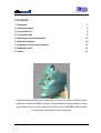
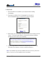
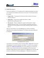
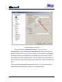
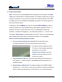
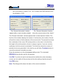
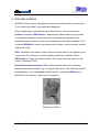
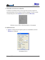
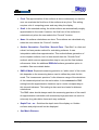
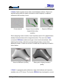
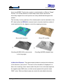
Version 3 (for Rhinoceros© 5)
User Manual
30 August 2013
Note: Please watch the tutorial video on www.rhinoreverse.icapp.ch as well!
© iCapp GmbH
Technoparkstrasse 1
8005 Zürich, Switzerland
[email protected]
rhinoreverse™ is a plug-in application for use with the Rhinoceros© CAD system
(www.rhino3d.com). It was designed to enable the user to create NURBS surfaces
efficiently based on given triangle meshes. With rhinoreverse, control point meshes can
be converted to NURBS surfaces. Boundary curves are sketched onto the mesh. All
calculations for the approximation and adaptation of the surface transitions are performed
automatically, resulting in a very simple and intuitive workflow. Rhinoreverse offers the
user the advantage of being able to represent large complex shapes very accurately with
only a few smooth surfaces. rhinoreverse can handle the following input formats:
*.stl, *.pol, *.wrl, *.vrml, *.af, *.nas
rhinoreverse is easy to use and is very cost-effective compared to other reverse
engineering programs. rhinoreverse is a product of iCapp GmbH.
Load mesh
Import surfaces
Sketch surfaces
Healing
Settings
Distance measurement
Patch
Redesign curves
New in Version 3
All significant results and improvements from our development up to now have been
incorporated in Version 3. And there’s more:
-
Distance measurements from the point cloud to the surface
-
Geometry-based curve redesign
iCapp GmbH, Technoparkstrasse 1, 8005 Zürich
www.rhinoreverse.icapp.ch, [email protected]
30 August 2013
2
Contents
1. Download
4
2. Install the plug-in
5
3. Launch Rhino 5
6
4. Load mesh data
8
5. Sketching surface boundaries
10
6. Calculate surfaces
14
7. Calculate curves/curve networks
15
8. Additional tools
15
9. Tables
21
Polylines (lines specified with a sequence of points) are drawn to divide a given
mesh into individual NURBS surfaces. The partitions should be placed as close
as possible to the curvature transitions of the surface. A NURBS surface will be
automatically calculated for each closed cell.
30 August 2013
3
1. Download
1. Ensure that Rhino 5 is installed on your computer before installing
rhinoreverse.
2. Download the installation file of rhinoreverse from the web-site
www.rhinoreverse.icapp.ch. A request form window will appear:
3. Please enter your email address, first name, last name and company and click
“Submit”. The Internet page address to download the software installation
package from will be sent to you immediately:
4. Click on the provided link and save the rhinoreverse.zip file to the C: drive
(hard disk) of the computer, you plan to install the software on.
Note: The installation may fail if the installation files are run from any other drive
letter, or if you try to run the installation across the network.
30 August 2013
4
2. Install the plug-in
Launch the installation file. The software will be installed automatically, provided
you've followed the installation instructions on the screen. The following files will
be installed:
•
Program files – The program file rhinoreverse.rhp is copied to the plug-in
directory of Rhino 5.
•
Sample files – These will be copied to the directory “Installpath\RhinoReverse\Example_Data”.
•
User manual – The file “UserManual_eng.pdf” will be copied to “Installpath\RhinoReverse\Tutorial”. The user manual is accessible via the Rhino
Help Menu and can be opened using the path Help/Plug-ins/Rhinoreverse in
Rhino 5.
When you launch Rhino 5, the rhinoreverse plug-in will be automatically
initialized and the toolbar will be displayed. The License Information window will
be displayed:
rhinoreverse license request
If you wish to try the software, click on the button Trial (..) days left. You may use
rhinoreverse for the period indicated on the button. If you want to buy a license,
please click on Mail License Request. An e-mail containing your node ID (the
number of your computer determined by rhinoreverse) will be automatically
generated. Please add any specific questions and suggestions you may have and
send the e-mail directly to [email protected]. iCapp will then generate a
30 August 2013
5
(paid) license key valid for use on your computer only and send it to you. Please
enter the issued license key in the LicenseKey field of the Licence Information
window and click on Register.
Note: You need to log in with administrative rights to install the software, because
the license key must be written to the Windows registry file. If the registration
fails, a message will be displayed. Log in as an administrator and repeat the
registration procedure.
3. Launch Rhino 5
Launch Rhino 5 as you would any other software, e.g., via the Windows “Start”
menu. rhinoreverse will be launched automatically and the toolbar will appear.
rhinoreverse toolbar
Once rhinoreverse function has been carried out, the menu item iCapp Tools
will be initialized and displayed in Rhino’s main menu.
Now make sure the command prompt window is shown. In the main menu
select Tools/Options, then select Rhino Options/Appearance and check the
option to show Command prompt.
30 August 2013
6
Check Absolute Tolerance
Then check Rhino’s Absolute Tolerance. To do so, select
Tools/Options and then Document Properties/Units. Adjust the tolerance
setting to match the size of your current model. If it is too small, rhinoreverse
will assign a high level of flexibility to the NURBS surfaces in order to reach
the transitional tolerance between them. This will lead to increased amount of
data to process, longer times required to calculate new surfaces and larger file
sizes.
We recommend setting absolute tolerance value to 0.01 when working with
models with dimensions around 1000 mm (see figure above).
30 August 2013
7
4. Load mesh data
Note: The functions of rhinoreverse can be accessed via the toolbar, the iCapp
Tools menu and the Rhino command window. The toolbar includes only the most
important commands. If you wish to work with the command window, enter “RR”
to display the list of all available rhinoreverse commands. The full list appears at
the end of this document.
In the menu, click LoadMesh (or enter the command RRLoadMesh) to open a
mesh file. Select any of the available Rhino mesh objects and press “Enter”, or
press the “f” key to read a mesh from a file. The following file formats are
available: *.stl (Stereo-Lithography), *.pol (PolyWork Version 1), *.wrl and *vrml.
The option “Delete input” is automatically set to YES. This is to avoid duplication
when displaying the mesh after converting it from Rhino to rhinoreverse.
Please note the following important points:
a. The given point cloud must be meshed. Point data without any
connections between the points (mesh data) cannot be used.
b. The picture shows a defective mesh.
The color of each triangle represents
the direction of its normal.
Neighboring triangles must have
identical normals and thus be the
same color as well.
c. Large amounts of data can slow down data display and processing. In
such cases (> 1 million triangles), rhinoreverse will automatically use a
simplified display.
d. Using inches as Model unit. The default setting for the “RMS of Mesh”
tolerance is 0.1. This value is correct if the model units used are millimetres
and for models with dimensions of 100-1000 mm. If a model dimensions
30 August 2013
8
are to be defined in inches (3.94 – 39.37 inches), the RMS tolerance must
be adjusted to 0.005.
The “General Information” window
The “General Information” window
appears after a mesh has been loaded
shows the current status of the “sketch”
The “General Information” window appears after a mesh has been loaded. The
first line of the window displays the number of vertices (#v), the number of facets
(#f) and the number of holes (#holes) of the current mesh. The second line shows
the coordinates of the current 3D mouse position on the mesh. In the third line,
the length of the active polyline, shown in orange (or green, if you are currently
modifying it with the mouse) is calculated. The fourth line shows the number of
patches and curves generated. In the last line you will find a Terminate button to
cancel the automatic calculation process.
Close this window to exit the rhinoreverse editing mode. The command
RREditGrid can also be used for this purpose.
Live Edit. If you do not want to set new points to define the surface boundary
curves, you can switch off the preview and thus the setting of points using the
Live Edit button.
Note: The dialogue title shows the status of the current calculation.
30 August 2013
9
5. Sketching surface boundaries
First, if working with mesh data, generated by measurement systems, please
adjust the rhinoreverse measuring tolerance parameters. If the tolerance value is
set too low, rhinoreverse may create a surface with "wrinkles. If the tolerance
value is set too high, the surfaces will not follow the mesh closely enough. Please
launch RROptions and adjust the RMS tolerance (RMS: root mean square
distance) accordingly (see also section 8).
Sample: “Head” The mesh data
(“Install-path\RhinoReverse\Sample_Files\Head_start.pol”), come from a laser
scanner; the measurement accuracy is approximately 0.25 mm. In this case the
RMS must be set to 0.25 (default is 0.1).
Sketch polylines
a. Make sure that the edit mode of rhinoreverse is active: The “General
Information” window (see section 4) must be open. The editing mode should
be activated immediately after mesh data are read. If it is not activated, click
on the menu item Edit Grid (command: RREditGrid) to activate the edit
mode.
b. Click anywhere on the mesh. The first point of a polyline (surface boundary
curve) will be generated and shown as a small red sphere.
30 August 2013
10
c.
Moving the mouse will generate a preview of the active polyline. The preview
shows the polyline, which would be generated if you set the next point by leftclicking.
The green line shows a
... the second point is set.
Option 1: When the mouse
preview of the curve. When
The curve has two points
is moved again a preview
the user clicks at the cursor
now. It automatically
of the whole curve is
becomes active (orange).
shown (green).
Option 2: If the angle of the
Clicking will set the second
Option 3: If the distance
mouse movement is more
point of the new curve. The
between the cursor and
new curve is now active
the last point is greater
(orange) the old one inactive
than the combined length
(gray).
of the last two curve
position...
than 60 degrees, a new
curve (green) will be started
at the last point of the first
one.
segments, left-clicking
creates a new curve.
How do I close a loop?
30 August 2013
11
If the cursor is close to an
... If the user then clicks the
... In this case, select
existing point, the point will
left mouse key, a menu will
“Snapping” to close the
be highlighted...
showing all available
loop and start the
options will be displayed.
calculation of the first
surface (gray).
Note: If polylines are not visible...
When the polylines are being drawn, an internal depth test mechanism (see
section 8) decides what is displayed and what is hidden. If a curve or a part of
the curve is behind the mesh, that part will not be displayed.
A complete grid is shown here.
Every closed loop of curves defines one surface (max. 25 curves).
When a closed loop is ready, the loop will be filled with one surface. Polylines
with only one point will be deleted automatically.
30 August 2013
12
Note: Curves that cross each other on the mesh surface without having a
common defined vertex could lead to problems when calculating a new
surface. Care must be taken to avoid crossing curves.
Note: The polylines that are used to define a closed loop must be connected
with common points. The respective start and end points may not be adjacent
to each other.
Note: Sometimes the displayed starting surfaces are not positioned exactly
over the mesh data. They will be pulled into their final position on the mesh in
the last approximation step (see section “Calculate surfaces”).
Edit polylines
a. Activate any polyline by clicking on it, or on a point of the polyline, with the left
mouse button. The active polyline is highlighted in orange.
Note: If you wish to activate the polyline, without activation any of its points,
please click on the line segment between the points.
b. Move single points of the active polyline by clicking and dragging them using
the mouse. When you release the mouse key, the point is dropped and
defined on the mesh.
c. Delete points. Activate the point to be deleted by left-clicking it (the point is
highlighted in red) and press the Delete button on your keyboard. Pressing
Delete again deletes the entire polyline.
d. Delete polylines. Activate the polyline (but not the point) by clicking on the
line segment between the points and press the Delete button. If no point was
activated (highlighted in red), the active polyline (highlighted in orange) will be
deleted.
e. Join/split polylines. Right-click the common point of the two polylines to join
them. Click on any point to split the polyline again. This is important
particularly when the surface boundary is to have sharp corners.
30 August 2013
13
6. Calculate surfaces
NURBS surfaces can be calculated only when the polylines form a closed loop.
Then a starting surface is generated and displayed.
When transferring intermediate surface data to Rhino, use the menu item
Commit (command: RRCommit) to approximate these surfaces on the mesh.
The transitions between the surfaces will be automatically adjusted to the
specified tolerance and the surface then transferred to the Rhino database. The
command RRRelief is used to generate a relief surface; see the section entitled
“Additional Tools”.
Note: Sometimes the display of the surfaces and the mesh is not optimal for the
current task. For this reason, various display modes are available. Select
RROptions to change the display options. See more about the options in the
section “Additional Tools”.
Transitions between surfaces. Rhino offers several options for analyzing
transitions between surfaces (e.g. in a typical zebra plot). If the resulting quality is
not satisfactory, use rhinoreverse´s Heal function (command: RRHeal) on a
selected set of surfaces to improve the transitions.
Zebra plot in Rhino
30 August 2013
14
7. Calculate curves/curve networks
In addition to calculating surfaces, the user also has the option to import the
generated polylines as curve entities to the Rhino database. To do this, use the
corresponding option of the Commit function (command: RRCommit.)
Wireframe curves in Rhino, defined by polylines in rhinoreverse
8. Additional tools
a. Options. A dialogue box with specific options for rhinoreverse (command:
RROptions) is displayed.
rhinoreverse Options
30 August 2013
15
•
Final. The approximation of the surfaces is done continuously, so that the
user can evaluate the final form of the surfaces at any time. This setting
requires a lot of computing power and may delay the display.
•
Draft. In the standard setting, the initial surfaces are automatically roughly
approximated to the mesh. However, the final form of the surfaces is
calculated only when the user selects the “Commit” function.
•
None. No surface calculations are done. The surfaces are calculated only
when the user selects the “Commit” function.
•
Surface Generation - Fast Skin / Smooth Face. “Fast Skin” is a fast and
robust, but less precise method for calculating surfaces. It uses
interpolation rather than approximation. This method allows generation of
more complex surfaces, but it is less smooth than the “Smooth Face”
method, which uses an approximation step to carry out the final surface
refinements. Note: An additional RRRelief surface generation option is
available. See more details below.
•
RMS of Mesh. Expected measuring precision or “white noise” of the mesh;
this depends on the measuring device used to define the points for this
mesh. The “measurment precision” is the tolerance range of the deviations
of the measured points from the real surface. In rhinoreverse the RMS
setting limits the approximation iterations up to a value corresponding to
this internal tolerance. This setting is also used as a basis for distance
calculations.
The RMS value should always match the measuring precision of the mesh!
An approximation calculation with excessively high precision can result in
extremely long calculation times and wavy surfaces.
•
Depth Test - on -. Switches the depth test of the display on. Hidden
surfaces and polylines will not be displayed.
•
Surf Mesh Distance.
30 August 2013
16
Note: This is an experimental option. Save your model before using this
option.
This option is used to calculate the distance between surfaces and the
mesh online. Please note that the “Final” option must also be activated.
When a polyline is edited, the associated surfaces are recalculated and the
distances to the mesh are displayed in colour. The colour shade depends
on the current setting for the RMS value of the mesh, as it is assumed that
the surface is approximated to the mesh up to this distance. The colour
goes from green to yellow to red. Green indicates the range between +/- 1
x RMS, yellow between +/- 2x RMS and red +/- 3 x RMS.
•
Surface display – Shade. – The initial surfaces are displayed with
shading.
•
Surface display – Hatch. -. The surfaces are represented only by their
iso-curves, allowing a transparent view of the mesh and the polylines.
•
Surface display – Outline. - Only the outlines are shown with an offset to
the inside. This option helps check whether all loops are closed as
required.
•
Surface display – CtrlPts. - The control polygons (control points and
control mesh) of the NURBS surfaces are displayed.
•
Surface display – none. – The surface display is completely switched off.
•
Edges. Switches the display of face edges on or off.
b. Special NURBS commands
1. Heal. All transitions of the selected set of surfaces are checked and the
absolute and angular precision values are adjusted automatically to match
those set within Rhino’s (command: RRHeal).
30 August 2013
17
2. Patch. Patch may be used to close a hole between surfaces. There is an
optional setting within the patch command to match tangency to adjacent
surfaces at the boundary curves.
Curve network
Support faces to define
Result of RRPatch
tangential boundary
condition
When designing surface models, users frequently need to fill in gaps between
already finished surfaces with a tangential surface. The menu item Patch
(command: RRPatch) enables such gaps to be closed automatically. After
selecting the function, select the corresponding boundary curves of the
adjacent surfaces. If these do not form a closed loop, the opening is closed in
linear fashion.
Result of RRPatch (4 times)
Zebra plot to display transition
quality
3. Relief. In geography and architecture, large relief surfaces are frequently
available only in STL format. The function RRRelief was developed to convert
30 August 2013
18
them into NURBS. This function works in a similar fashion to Rhino’s “Drape”
function. The crucial difference is that steep surface areas can also be
accurately mapped: the control points are evenly distributed throughout the
surface.
The boundary curves (polylines) of the desired patch must be sketched on the
STL data before the RRRelief command can be launched and the number of
control points set for the edges to control the mapping accuracy.
Given relief structure
Given STL surface
Resulting NURBS (200 control points
Resulting NURBS (shaded view)
in the long edge)
4. Mesh-face Distance. The approximated surface is analyzed at a distance
to the reference “point cloud”. The result of the calculation is displayed in a
false color rendering. Green areas match the point cloud, red areas represent
the negative triple RMS value, and blue areas represent the positive triple
“RMS” value. White and black areas are outside the calculated tolerances.
30 August 2013
19
Topological details can be analyzed in greater detail by changing the RMS
settings and recalculating.
Several areas can be selected for distance measurement. In this case a
separate mesh is calculated in order to display each surface.
The false color rendering is a separate mesh. It can be moved to a separate
level for documentation if necessary.
5. Redesign curves. The redesign of curves is always strictly geometry-based.
The maximum allowed distance can be freely selected. The best possible result is
determined by the control point distribution. The objective is always the largest
possible reduction of control points.
30 August 2013
20
9. Tables
Commands relating to the mesh and the generation of polylines:
Tool
Menu Item
Command
Description
Load Mesh
RRLoadMesh
Imports a Rhino mesh object or opens a
mesh file
Edit Grid
RREditGrid
Switches on the display for the polylines
belonging to the current mesh. “Edit Mode”
is activated.
Commit
RRCommit
The surfaces are approximated and the
transitions adjusted. Then the surfaces or
curves are transferred to the Rhino
database.
Options
RROptions
Sets tolerances and display options.
-
Hide Mesh
RRHideMesh
Hides or shows the mesh object
-
ImportGridV1
RRImportGridV1
Enables the import of polylines generated
and saved with rhinoreverse version 1
-
Relief
RRRelief
Fast method of “draping” a specific area of
a given point mesh with one NURBS
surface
30 August 2013
21
Additional tools which work on NURBS:
Heal
RRHeal
All transitions of a selected set of surfaces
are adjusted automatically to conform to
Rhino's “Absolute Tolerance” and “Angular
Tolerance”
Patch
RRPatch
Covers a hole enclosed by an open or
closed loop of selected surface boundary
curves.
Mesh-Face
Distance
Curve
RRMeshFaceDis
tance
RRCurve
Calculates the distance from the
approximated surface to the given mesh.
New approximation of the curve depending
on the given geometry
30 August 2013
22