Download User Manual

GiD
The universal, adaptative and user
friendly pre and postprocessing
system for computer analysis
in science and engineering
User Manual
ii
Table of Contents
Chapters
Pag.
1 INTRODUCTION
1.1 Models used in this manual
2 INITIATION TO GiD
2.1 User interface
1
1
3
3
2.1.1 Change theme
3
2.1.2 Warnline
4
2.1.3 Command line
4
2.1.4 Status bar
4
2.1.5 Contextual menu
5
2.1.6 Escape function
6
2.2 Load a model
6
2.3 Render modes
7
2.4 Change views of the model
9
2.4.1 Zoom
9
2.4.2 Pan
9
2.4.3 Rotate
2.4.3.1 Set center of rotation
2.5 Layers and groups
10
10
10
2.5.1 Create a layer
11
2.5.2 Rename a layer
11
2.5.3 Change the color of a layer
12
2.5.4 Send entities to a layer
12
2.5.5 Switch On/Off
14
2.5.6 Freeze a layer
14
2.5.7 Transparency
14
2.6 Entities information
15
2.6.1 Labels
15
2.6.2 List entities
16
2.6.3 Signal
17
2.7 Geometry and Mesh modes
18
2.8 Pre and Post
19
Table of Contents
2.9 Select and display style
3 INITIATION TO PREPROCESSING
iii
19
23
3.1 First steps
23
3.2 Creation and meshing of a line
24
3.3 Creation and meshing of a surface
28
3.4 Creation and meshing of a volume
37
4 IMPLEMENTING A MECHANICAL PART
4.1 Working by layers
43
43
4.1.1 Defining the layers
43
4.1.2 Creating two new layers
44
4.2 Creating a profile
44
4.2.1 Creating a size-55 auxiliary line
44
4.2.2 Dividing the auxiliary line near coordinates (40, 0)
45
4.2.3 Creating a 3.8-radius circle around point (40, 0)
46
4.2.4 Rotating the circle -3 degrees around a point
46
4.2.5 Rotating the circle 36 degrees around a point and copying it
47
4.2.6 Rotating and copying the auxiliary lines
48
4.2.7 Intersecting lines
51
4.2.8 Creating an arc tangential to two lines
53
4.2.9 Translating the definitive lines to the "profile" layer
53
4.2.10 Deleting the "aux" layer
54
4.2.11 Rotating and obtaining the final profile
54
4.2.12 Creating a surface
55
4.3 Creating a hole in the mechanical part
4.3.1 Creating a hole in the surface of the mechanical part
4.4 Creating volumes from surfaces
4.4.1 Creating the "prism" layer and translating the octagon to this
56
57
58
58
layer
4.4.2 Creating the volume of the prism
59
4.4.3 Creating the volume of the wheel
60
4.5 Generating the mesh
61
4.5.1 Generating a coarse mesh
61
4.5.2 Generating the mesh with assignment of size around points
64
4.5.3 Generating the mesh with assignment of size around lines
66
5 IMPLEMENTING A COOLING PIPE
69
Table of Contents
iv
5.1 Working by layers
69
5.2 Creating a component part
70
5.2.1 Creating the profile
70
5.2.2 Creating the surfaces by revolution
70
5.2.3 Creating the union of the main pipes
71
5.2.4 Copying the main pipe
72
5.2.5 Creating the end of the pipe
73
5.3 Creating the T junction
75
5.3.1 Creating one of the pipe sections
75
5.3.2 Creating the other pipe section
76
5.3.3 Creating the lines of intersection
77
5.3.4 Deleting surfaces and close a volume
77
5.4 Importing the T junction to the main file
78
5.4.1 Importing a GiD file
78
5.4.2 Creating the final volume
79
5.5 Generating a mesh
80
6 ASSIGNING MESH SIZES
83
6.1 Introduction
6.1.1 Reading the initial project
6.2 Element-size assignment methods
83
83
84
6.2.1 Assign general mesh size witth default options
85
6.2.2 Assign size to points
86
6.2.3 Assign size to lines
88
6.2.4 Assign size to surfaces
89
6.2.5 Assignment following chordal error criterion
90
6.3 Rjump mesher
91
6.3.1 RJump default options
92
6.3.2 Force to mesh some entity
93
7 METHODS FOR MESH GENERATION
7.1 Introduction
7.1.1 Reading the initial project
7.2 Types of mesh
7.2.1 Generating the mesh by default
7.2.2 Generating the mesh using circles and spheres
97
97
97
98
99
100
Table of Contents
v
7.2.3 Generating the mesh using points
101
7.2.4 Generating the mesh using quadrilaterals
102
7.2.5 Generating a structured mesh (surfaces)
103
7.2.6 Generating structured meshes (volumes)
105
7.2.7 Generating semi-structured meshes (volumes)
107
7.2.8 Concentrating elements and assigning sizes
109
7.2.9 Generating the mesh using quadratic elements
111
8 POSTPROCESSING
115
8.1 Loading the model
115
8.2 Changing mesh styles
116
8.3 Viewing the results
117
8.3.1 Iso surfaces
119
8.3.2 Animate
120
8.3.3 Result surface
121
8.3.4 Contour fill, cuts and limits
123
8.3.5 Combined results
126
8.3.6 Stereo mode (3D)
128
8.3.7 Show Min Max
129
8.3.8 Stream lines
130
8.3.9 Graphs
133
8.4 Creating images
137
9 CAD CLEANING OPERATIONS
141
9.1 Importing on GiD
141
9.1.1 Importing an IGES file
9.2 Correcting errors in the imported geometry
142
144
9.2.1 Meshing by default
144
9.2.2 Correcting surfaces
146
9.3 The conformal mesh and the non-conformal mesh
149
9.3.1 Global collapse of the model
149
9.3.2 Correcting surfaces and creating a conformal mesh
151
9.3.3 Creating a non-conformal mesh
157
10 DEFINING A PROBLEM TYPE
10.1 Introduction
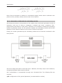
10.1.1 Interaction of GiD with the calculating module
159
159
160
Table of Contents
10.2 Implementation
vi
162
10.2.1 Creating the Materials File
162
10.2.2 Creating the General File
164
10.2.3 Creating the Conditions File
164
10.2.4 Creating the Data Format File (Template file)
165
10.2.5 Creating the Execution file of the Calculating Module
171
10.2.6 Creating the Execution File for the Problem Type
172
10.3 Using the problemtype with an example
10.3.1 Executing the calculation with a concentrated weight
10.4 Aditional information
10.4.1 The main program
174
176
177
178
1
1 INTRODUCTION
This manual contains a collection of tutorials and practical information for learning the
basics and advanced features of GiD, covering full flow of GiD user from preprocessing to
postprocessing going trough meshing, analysis and introduction to customization.
1.1 Models used in this manual
In order to follow some of the tutorials included in this manual some files should be
downloaded.
The models are located in GiD official webpage www.gidhome.com in Support->Manuals
section.
The models are packed in a zip file and classified by chapters.
INITIATION TO GiD
2
3
2 INITIATION TO GiD
The philosophy of this tutorial is to get familiarized with GiD: how to change the views of
the model, how to manage the Layers, and other basic features. Some of this features are
both in the preprocessing and the postprocessing parts of GiD, although the examples
shown are from the preprocessing one.
Many times the text will make reference to 'entities'. Almost all the options explained in this
tutorial are valid both for geometrical and mesh entities, although the examples used are
often geometrical ones.
The topics in this tutorial are further explained in the Reference Manual. We have
selected some of the basic features to give to the user some basic tips to start working with
GiD and make the rest of the tutorials.
2.1 User interface
For further information about GiD user interface please consult the General aspects->User
interface section in the Reference manual.
2.1.1 Change theme
User can choose between Classic and Dark themes, which change drastically the GUI
appearance. User can also choose between some icon sizes in each theme.
Change theme
4
These options can be changed in GiD Theme option inside
Utilities->Preferences->Graphical->Appearance tab.
2.1.2 Warnline
In some of the operations made in GiD by the user, GiD gives information about what is
expected to do by the user. This information is very useful the first times GiD is used as a
guideline for the user.
The place were GiD shows this kind of information is the lower part of its main window.
2.1.3 Command line
Using GiD,
sometimes the user is asked to
introduce data with the
keyboard. The
'Command line' must be used for this purpose. It is placed in the lower part of GiD window.
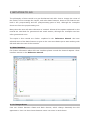
2.1.4 Status bar
The Status & Information bar located at lower part of GiD's Window, provides basic
information at a quick glance.
From left to right you can find:
Zoom factor
Current number of nodes and elements (Click to acces to Status Window)
Status bar
5
Current renter mode (Click to change render)
Number of layers in Pre, number of sets in Post
Mouse coordinates (Click to open "Coordinate window" in Pre and "Change result units"
in Post)
Current Mode: Pre or Post
2.1.5 Contextual menu
Clicking the right-mouse button on GiD a popup menu will appear with options related to
the clicked object.
When picking the main drawing space, on the top appear Contextual that is filled with
different commands depending on the current GiD state, e.g. when asking for a point they
appear options like "Point in line", to select a point over a line, or "Arc center" to select the
coordinates of the center of an arc.
Contextual menu
6
2.1.6 Escape function
An important thing a GiD user should know as a general philosophy of use of the program
is the Escape key functionality: In almost all the actions performed by the user, to declare
the action as done the user should press Escape key (or press the center mouse button).
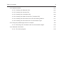
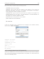
2.2 Load a model
In the Files menu user can find the typical operations for managing the GiD projects like
save a project, open an existing project, import and export files, print or quit the program.
Most of this options are also accessible from the icons toolbar. The corresponding icon is
shown in the menu, next to the option.
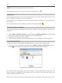
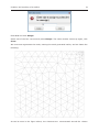
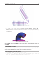
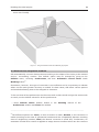
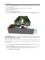
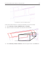
1 . Click on Files->Open... and select the GiD model gid_model_basic.gid. GiD also
can load a model just with drag & drop.The following model should be loaded:
Load a model
7
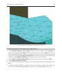
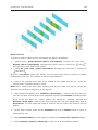
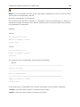
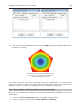
2.3 Render modes
In the View menu user can find the Render options. They are also accessible from the
right mouse button and the status bar.
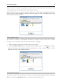
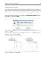
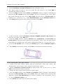
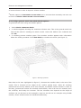
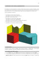
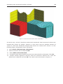
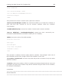
1 . Select View->Render->Normal
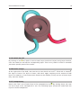
In Normal render mode, user can see the entities drawn in different colors, depending on
the kind of entity: volumes in light blue, surfaces in pink, lines in blue, and points in black,
as it can be seen in the following figure:
Render modes
8
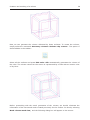
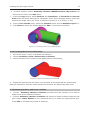
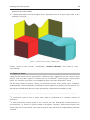
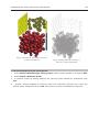
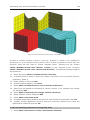
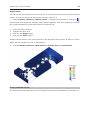
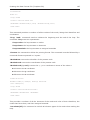
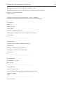
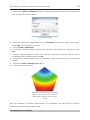
2 . Select View->Render->Flat
3 . Select View->Render->Smooth
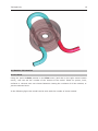
Flat render mode draws each geometrical entity using the colour of the layer it belongs to,
and Smooth mode uses also this criterion, but lines are not drawn to represent the
geometry in a smoother way. The following figure shows the visualization of the model
using 'Smooth' render mode:
Render modes
9
2.4 Change views of the model
In the View menu user can find the options to change the point of view in which the model
is shown. Many of these options are also accessible by the right mouse button menu, or the
icons toolbar.
2.4.1 Zoom
To zoom in or out the model user can
choose the
corresponding
options in the
Zoom section of the View menu or the right mouse button menu.
A user friendly way of zooming the model is to use the wheel of the mouse, or clicking the
center button of the mouse while the Shift key is pressed.
To get a view which includes the whole model the Frame option must be selected.
The icons corresponding the zoom operations are the following ones:
Zoom in:
Zoom out:
Zoom frame:
2.4.2 Pan
To move the view of the model user must select the option Pan. This option is accessible
from the View menu, the right mouse button menu, or moving the mouse while the
Pan
10
Shift key and the right mouse button are pressed.
The corresponding icon for the pan option is the following one:
2.4.3 Rotate
In the 'Rotate' part of the 'View' menu (also present in the right mouse button menu) there
are the options to rotate the view of the model.
A user friendly way of rotating is to move the mouse while its left button and the 'Shift' key
are pressed.
The corresponding icon for rotating the model is the following one:
2.4.3.1 Set center of rotation
An interesting option for rotating the view of the model is to set the center of rotation. To
change it:
1 . Select View->Rotate->Center from top menu or Rotate->Center from right button
mouse menu. Then, the cursor changes into the selection mode.
2 . Select an existing point of the model.
3 . Now rotate the model and check that the center of the rotation is the one selected.
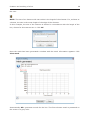
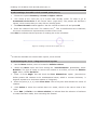
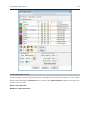
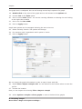
2.5 Layers and groups
A really useful way for organizing the different parts of the model is using 'Layers'.
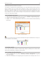
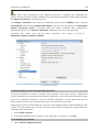
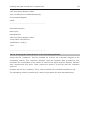
1 . Open the Layers window by selecting the Utilities->Layer and groups option or
clicking
in the upper icons toolbar. The following window should raise up:
As it can be read in the upper part of the window, if user double click on that part, the
Layers window is integrated in GiD window. User can choose to work with the Layers and
groups window integrated or not.
All the actions related with layers and groups can be accessed by clicking the right mouse
Layers and groups
11
button onto the Layers and groups window. Most of them can be also used by the
corresponding icon in the upper part of the Layers window.
By moving the mouse over the icons of the upper part of the window and staying 2 seconds
onto an icon, a help message is shown in order to give the user information about the
action associated with the icon.
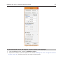
2.5.1 Create a layer
GiD allows to create a
hierarchical
structure of Layers, so as a Layer can contain
sub-layers. Let's create a Layer into another one as an example:
1 . Select (using the left button of the mouse) the 'Layer6'.
2 . Select the New child option in the right mouse button menu, or click
in the upper
part of the Layers and groups window. Automatically, a layer named 'Layer0' should
appear, as shown in the following figure:
2.5.2 Rename a layer
To rename a Layer user should select the layer in the Layers and groups window and press
F2 key, or select the Rename option in the right mouse button menu.
Rename a layer
12
1 . Select the Layer0
2 . Rename it to 'Auxiliar'
Now the Layers window should look like the following picture:
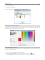
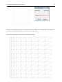
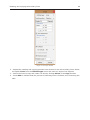
2.5.3 Change the color of a layer
By clicking on the colored square next to each layer name, the following window pops-up,
allowing the user to change the color of the layer:
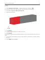
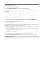
2.5.4 Send entities to a layer
User can send entities to a specific layer. As an example we are going to send to the layer
'Auxiliar' a part of the model:
1 . Select the layer 'Auxiliar' in the Layers window
2 . Select the option Send to from the right mouse button (or click
icon)
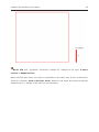
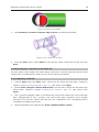
3 . Select Volumes and select the volume shown in red in the following figure:
Send entities to a layer
13
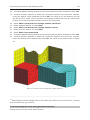
4 . Then press Escape to exit the selection mode.
5 . Set the render mode to Flat. The color of selected volume has changed to the one of
the layer 'Auxiliar', as shown in the following figure:
Send entities to a layer
14
2.5.5 Switch On/Off
By clicking on the icon which is next to each Layer inside the Layers and groups window,
user can switch on and off the corresponding layer. This is very useful in order to visualize
just some specific parts of the model.
2.5.6 Freeze a layer
At the right side of the bulb, user can set an icon which is a lock
. If the lock is closed ,
the layer is frozen. If a layer is frozen, GiD won't apply anything to the entities of that
layer. For instance, if user select some entities to be deleted, if they are into a frozen layer
they won't be erased.
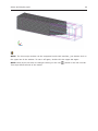
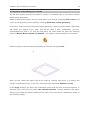
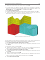
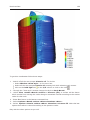
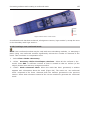
2.5.7 Transparency
Next to the 'lock' icon of each layer is the transparency icon . By clicking there, the user
can set a layer to be transparent or not. The following figure shows the model with the
Layer11 set as transparent:
Transparency
15
2.6 Entities information
2.6.1 Labels
Using the option Labels present in the View menu (and also in the right mouse button
menu), user can see the number of the entities of the model. Either for points, lines,
surfaces or volumes user can choose between viewing the numbers of all the entities, or
just the selected ones.
In the following figure the model can be seen with the number of some entities:
Labels
16
As it can be seen, the colors of the numbers of the entities follows the philosophy of the
colors of the entities in GiD (volume numbers are in light blue, surface numbers are in pink
and so on).
In order to get a better visualization set the render mode to normal when showing labels.
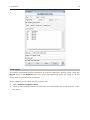
2.6.2 List entities
User have also the option of viewing all the characteristics of a specific entity by selecting
List in the Utilities menu (or clicking
in the icons toolbar).
For example:
1 . Select Utilities->List->Surfaces in the top menu
2 . Select some surfaces of the model
3 . Press Escape
An example of the information got using this option is the following figure:
List entities
17
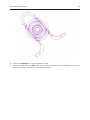
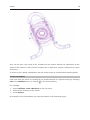
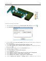
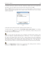
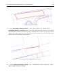
2.6.3 Signal
In complex geometrical models sometimes it is hard to localize an specific entity. Using the
Signal option in the Utilities menu user can know graphically where the entity is, as GiD
shows with a red lines cross its potition.
As an example we will signal the line number 290:
1 . Selec Utilities->Signal->Lines
2 . Write in the Command bar the number 290 and click ENTER. The result is shown in the
next figure:
Signal
18
The red lines are centered always onto the specific entity independently on the rotations or
view movements.
2.7 Geometry and Mesh modes
In the
preprocessing part of GiD there are two basic modes the user can work with:
geometry and mesh. Just in order to see how the mode can be changed we are going to
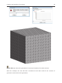
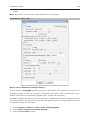
generate a mesh with all the default parameters.
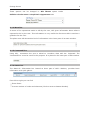
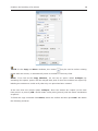
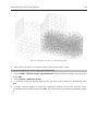
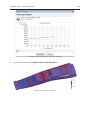
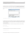
1 . Select Mesh->Generate mesh... The following window should appear.
2 . Click OK and wait for the mesh generation. Once the mesh is generated, a window
pops up and show the user the result from the mesh generation.
3 . Click on 'View mesh' option, and the following visualization of the model should
appear:
Geometry and Mesh modes
19
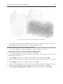
Now we are in 'mesh' mode. Changing the render mode user can see that the color of the
mesh entities also follows the Layer colors.
Selecting View->Mode->Geometry user can change to the geometry mode again. The
icon in the toolbar switch between both modes
2.8 Pre and Post
GiD basically works in two modes: preprocessing and postprocessing.
To
change
between
both
modes
Files->Preprocess (or clicking
please
select
Files->Postprocess or
in the upper toolbar).
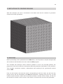
We will use a different model to work in postprocess mode.
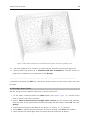
1 . Open the box3D.gid project
2 . Select Files->Postprocess
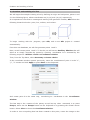
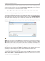
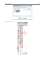
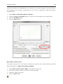
2.9 Select and display style
Through the Select & Display Style window several options can be specified for volumes,
surfaces and cuts. Among these options volumes, surfaces and cuts can be switched on and
off, their colour properties can be changed, and their transparency too.
Other interesting options which can be changed are the style of the set and the width of the
elements' edges.
From this window, volumes, surfaces or cuts can be deleted or their names can be
Select and display style
20
modified.
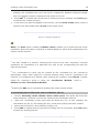
1 . Select Window->View style... using the menu bar or clicking on
Our model only has 1 layer. We will create a new layer with some elements.
2 . Press button Send to->New set long name.
3 . Select some elements.
4 . Press Escape.
5 . A window appears asking for a name. Enter 'Aux'.
6 . Press Accept.
A new layer is created with the selected elements. Now we will change the color of the new
layer.
7 . Click on the colored square next to the layer name. A new window is opened. Select a
new color.
8 . Press Apply and then Close.
Select and display style
21
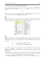
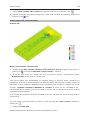
Let's play with some visualization options
9 . Select Body Lines in the "Style" option, at the bottom of the window. You can also do
it clicking on
in the St column or the same icon in the main window.
10 . Click on the icon of 'Aux' layer in order to switch it off.
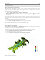
It's possible to draw preprocessing information, for example the geometry.
11 . In Draw Model option select Geometry
Now our model should look like this:
Select and display style
22
NOTE: The View style window can be integrated inside GiD interface, just double click on
the upper bar of the window. To tear it off again, double click the upper bar again.
NOTE: Mesh styles can also be changed clicking on the icon
This style affects all sets of the model.
, placed in the left icon bar.
23
3 INITIATION TO PREPROCESSING
With this example, the user is introduced to the basic tools for the creation of geometric
entities and mesh generation.
3.1 First steps
Before presenting all the possibilities that GiD offers, we will present a simple example that
will introduce and familiarize the user with the GiD program.
The example will develop a finite element problem in one of its principal phases, the
preprocess, and will include the consequent data and parameter description of the problem.
This example introduces creation, manipulation and meshing of the geometrical entities
used in GiD.
First, we will create a line and the mesh corresponding to the line. Next, we will save the
project and it will be described in the GiD data baseform. Starting from this line, we will
create a square surface, which will be meshed to obtain a surface mesh. Finally, we will use
this surface to create a cubic volume, from which a volume mesh can then be generated.
Creation and meshing of a line
24
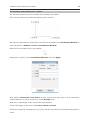
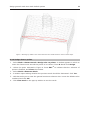
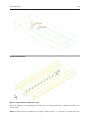
3.2 Creation and meshing of a line
We will begin the example creating a line by defining its origin and end points, points 1 and
2 in the following figure, whose coordinates are (0,0,0) and (10,0,0) respectively.
It is important to note that in creating and working with geometric entities, GiD follows the
following hierarchical order: point, line, surface, and volume.
To begin working with the
program, open GiD, and a new GiD project is created
automatically.
From this new database, we will first generate points 1 and 2.
Next, we will create points 1 and 2. To do this, we will use an Auxiliary Window that will
allow us to simply describe the points by entering coordinates. It is accessed by the
following sequence: Utilities->Tools->Coordinates window
Then, from the Top Menu, select Geometry->Create->Point
In the coordinate window opened previously, enter the coordinates of point 1 in the "x",
"y", "z" entries and click Apply or press Enter on the keyboard.
And create point 2 in the same way, introducing its coordinates in the
Coordinates
window.
The last step in the creation of the points, as well as any other command, is to press
Escape, either via the Escape button on the keyboard or by pressing the central mouse
button. Select Close to close the Coordinates window.
In order to view everything that has been created to this point, center the image on the
Creation and meshing of a line
25
screen by choosing in the Mouse Menu: Zoom->Frame.
Now, we will create the line that joins the two points. Choose from the Top Menu:
Geometry->Create->Straight line. Option in the Toolbar shown below can also be
used.
Next, the origin point of the line must be defined. In the Mouse Menu, opened by clicking
the right mouse button, select Contextual->Join Ctrl-a.
NOTE: It is important to note that the Contextual submenu in the Mouse Menu will always
offer the
options of the
command that is
currently being used. In this case, the
corresponding submenu for line creation, has the following options:
NOTE: With option Join, a point already created can be selected on the screen. The
command No Join is used to create a new point that has the coordinates of the point that is
selected on the screen. We can see that the cursor changes form for the Join and No Join
commands.
Now, choose on the screen the first point, and then the second, which define the line.
Finally, press Escape to indicate that the creation of the line is
completed. Press
Escape again to end the line creation function, if you don't press Escape you can continue
creating lines.
Once the geometry has been created, we can proceed to the line meshing. In this example,
this
operation will be
presented in the simplest and most
automatic way that GiD
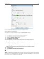
permits. To do this, from the Top Menu select: Mesh->Generate mesh.
And an Auxiliary Window appears, in which the size of the elements should be defined by
Creation and meshing of a line
26
the user.
NOTE: The size of an element with two nodes is the length of the element. For, surfaces or
volumes, the size is the mean length of the edge of the element.
In this example, the size of the element is defined in concordance with the length of the
line, chosen for this case as size 1. Click OK.
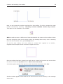
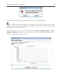
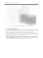
Once the mesh has been generated a window with the mesh information appears. Click
View mesh.
Automatically GiD generates a mesh for the line. The finite element mesh is presented on
the screen in a grey color.
Creation and meshing of a line
27
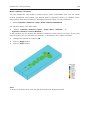
The mesh is formed by ten linear elements of two nodes. To see the numbering of the
nodes and mesh elements, select from the Mouse Menu: Label->All, and the numbering
for the 10 elements and 11 nodes will be shown, as below.
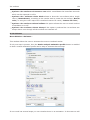
Once the mesh has been generated, the project should be saved. To save the example
select from the Top Menu: Files->Save.
The program automatically saves the file if it already has a name. If it is the first time the
file has been saved, the user is asked to assign a name. For this, an Auxiliary Window
will appear which permits the user to browse the computer disk drive and select the
location in which to save the file. Once the desired directory has been selected, the name
for the current project can be
entered in the space titled File Name. Save it as
initiation.gid.
NOTE: Next, the manner in which GiD saves the information of a project will be explained.
GiD creates a directory with a name chosen by the user, and whose file extension is .gid.
GiD creates a set of files in this directory where all the information generated in the
present example is saved. All the files have the same name of the directory to which they
belong, but with
different
extensions. These files should have the name that GiD
designates and should not be changed manually.
Each time the user selects option save the database will be rewritten with the new
information or changes made to the project, always maintaining the same name.
To exit GiD, simply choose Files->Quit.
To access the project that we have just created, simply open GiD and select from the Top
Menu: Files->Open. An Auxiliary Window will appear which allows the user to access
and open the directory initiation.gid.
Creation and meshing of a surface
28
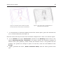
3.3 Creation and meshing of a surface
We will now continue with the creation and meshing of a surface.
First, we will create a second line between points 1 and 3.
We will now generate the second line. We will now use again the Coordinates Window to
enter the points. (Utilities->Tools->Coordinates Window)
Select the line creation tool in the toolbar.
Enter point (0,10,0) in the Coordinates Window and click Apply.
With option Contextual->Join Ctrl-a (mouse menu) click over point 1. A line should be
created between (0,10,0) and (0,0,0). Press Escape twice.
With this, a right angle of the square has been defined.
Center the image in the screen with View->Zoom->Frame.
Finish the square by creating point (10,10,0) and the lines that join this point with points 2
and 3.
Creation and meshing of a surface
29
Now, we will create the surface that these four lines define. To do this, access the create
surface command by choosing:
Geometry->Create->NURBS surface->By contour.
This option is also available in the toolbar:
GiD then asks the user to define the 4 lines that describe the contour of the surface. Select
the lines using the cursor on the screen, either by choosing them one by one or selecting
them all with a window. Next, press Escape twice.
As can be seen
below, the new
surface is
created and
appears as a
smaller,
magenta-colored square drawn inside the original four lines.
Once the surface has been created, the mesh can be created in the same way as was done
for the line. From the Top Menu select: Mesh->Generate mesh.
A window appears asking if the previous mesh should be elliminated. Click Yes.
Another window appears which asks for the maximum size of the element, in this example
defined as 1.
Creation and meshing of a surface
30
We can see that the lines containing elements of two nodes have not been meshed. Rather
the mesh generated over the surface consists of planes of
three-nodded, triangular
elements.
NOTE: GiD meshes by default the entity of highest order with which it is working.
GiD allows the user to concentrate elements in specified geometry zones. Next, a brief
example will be presented in which the elements are concentrated in the top right corner of
the square.
This operation is realized by assigning a smaller element size to the point in this zone than
for the rest of the mesh. Select the following sequence: Mesh->Unstructured->Assign
sizes on points. The following dialog box appears, in which the user can define the size:
Creation and meshing of a surface
31
Enter 0.1 and click Assign.
Select one of the four corners and press Escape. The same window comes up again, click
Close.
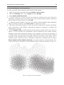
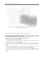
We must now regenerate the mesh, erasing the mesh generated earlier, and we obtain the
following:
As can be seen in the figure above, the elements are concentrated around the chosen
Creation and meshing of a surface
32
point. Various possibilities exist for controlling the evolution of the element size, which will
be presented later in the manual.
To generate a surface mesh in which the elements are presented uniformly, the user can
select the option for a structured mesh. This guarantees that the same number of elements
appears around a node and that the element size is as uniform as possible. To generate
this type of mesh, choose: Mesh->Structured->Surfaces->Assign number of cells.
Using this command, the user should first select the 4-sided NURBS surface that will be
defined by the mesh and press ESC.
Then a window appears where the number of subdivisions for the surface limit lines should
be entered.
Enter 10 and click Assign and select one of the horizontal lines, the parallel line is also
selected. Press ESC.
The same window appears again, click Assign and select one of the vertical lines, the
parallel one is also selected. Press ESC.
Click Close when the window appears again.
The number of divisions can be checked selecting Mesh->Draw->Num of divisions. To
exit this visualization mode press ESC.
Creation and meshing of a surface
NOTE: GiD only
generates
33
structured meshes for surfaces of the type 4-sided
surface or NURBS surface.
When this has been done, the mesh is generated in the same way as the unstructured
mesh, by choosing Mesh->Generate mesh. Erase the old mesh and assign a general
element size of 1, though in this case it is not necessary.
Creation and meshing of a surface
NOTE:
Another
way
to
get
34
the
same
result is
using
the
option
Mesh->Structured->Surfaces->Assign size. With this option we set the element size.
If we want to get 10 elements per line and the line measures 10 units, we should set 1 as
size.
If
we
don't
know
how
much
measures a
line
we
can
use
the
option
Utilities->Distance and select the 2 points defining the line.
We can see here that the default element type used by GiD to create a structured mesh is
a square element of four nodes rather than a three-nodded, triangular element. To obtain
triangular elements, the user can specifically define this type of element, by choosing
Mesh->Element
type->Triangle, and selecting the surface to mesh as a triangular
element. Regenerate the mesh, and the following figure is obtained:
Creation and meshing of a surface
35
GiD also allows the user to concentrate elements in structured meshes. This can be done
by selecting Mesh->Structured->Lines->Concentrate elements.
First, we must select the lines that need to be assigned an element concentration weight.
The value of this weight can be either positive or negative, depending on whether the user
wants to concentrate elements at the beginning or end of the lines. Next, a vector appears
which defines the start and end of the line and which helps the user assign the weight
correctly.
We want to concentrate the elements in the left zone of the square.
Select both horizontal lines and press ESC. A window appears to enter the weights values.
Both lines should have the same direction so enter a weight of 0.5 to the beginning of the
line and click Ok. Press ESC again to leave the function.
Creation and meshing of a surface
36
If lines have different direction, to obtain the same result, we should assign the weight for
one line to the beginning and to the end for the other line.
From these operations, we obtain the following mesh:
Creation and meshing of a volume
37
3.4 Creation and meshing of a volume
We will now present a study of entities of volume. To illustrate this, a cube and a volume
mesh will be generated.
Without leaving the project, save the work done up to now by choosing Files->Save, and
return to the geometry last created by choosing Geometry->View geometry.
In order to create a volume from the existing geometry, firstly we must create a point that
will define the height of the cube. This will be point 5 with
coordinates
(0,0,10),
superimposed on point 1. To view the new point, we must rotate the figure by selecting
from the Mouse Menu: Rotate->Trackball. This option is also available in the toolbar:
Rotate the figure until the following position is achieved and press ESC:
Next, we will create the upper face of the cube by copying from point 1 to point 5 the
surface created previously. To do this, select the copy command, Utilities->Copy.
In the Copy window, we define the translation vector with the first and second points, in
this case (0,0,0) and (0,0,10). Option Do extrude surfaces must be selected; this option
allows us to create the lateral surfaces of the cube. Fill in the rest of variables as shown in
the following image.
Creation and meshing of a volume
NOTE: In the Copy and Move windows, the button
38
may be used to select existing
points with the mouse, or alternativelly enter its number in the entry field.
NOTE: If we look at the Copy Window, we can see an option called Collapse. By
activating this option, point 6 will be merged with point 5 when the entities are copied. By
labeling the entities we could verify that only one point has been created.
If the user does not choose option Collapse, when the entities are copied (in this case
from point 1 to point 5) GiD would create a new point (point 6) with the same coordinates
as point 5.
To finish the copy command click Select, select the surface and then press ESC. We obtain
the following surfaces:
Creation and meshing of a volume
39
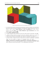
Now, we can generate the volume delimited by these surfaces. To create the volume,
simply select the command Geometry->Create->Volume->By contour . This option is
also available in the toolbar:
Select all the surfaces and press ESC twice. GiD automatically generates the volume of
the cube. The volume viewed on the screen is represented by a cube with an interior color
of sky blue.
Before proceeding with the mesh generation of the volume, we should eliminate the
information of the structured mesh created previously for the surface. Do this by selecting
Mesh->Reset mesh data, and the following dialog box will appear on the screen:
Creation and meshing of a volume
40
In which the user is asked to confirm the erasure of the mesh information.
NOTE:
Another valid option would be to assign a size of 0 to all entities. This would
eliminate all the previous size information as well as the information for the mesh, and the
default options would become active.
Next, generate the mesh of the volume by choosing Mesh->Generate mesh. Another
Auxiliary Window
appears into which the size of the volumetric element must be
entered. In this example, the value is 1.
Creation and meshing of a volume
41
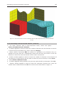
The mesh generated above is composed of tetrahedral elements of four nodes, but
GiD also permits the use of hexahedral, eight-nodded structured elements.
We will generate a structured mesh of the volume of the cube. This is done by selecting
Mesh->Structured->Volumes->Assign number of cells.
Now select the volume to mesh and press ESC.
Then a window appears where the number of subdivisions for the volume limit lines should
be entered.
Enter 10 and click Assign and select one of the lines in X axis, the parallel lines are also
selected. Press ESC.
The same window appears again, click Assign and select one of the lines in Y axis, the
parallel ones are also selected. Press ESC.
Again click Assign and select one of the lines in Z axis, the parallel ones are also selected.
Press ESC.
Click Close when the window appears again.
Then, create again the mesh.
Creation and meshing of a volume
42
NOTE: GiD only allows the generation of structured meshes of 6-sided volumes.
With this example, the user has been introduced to the basic tools for the creation of
geometric entities and mesh generation.
43
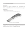
4 IMPLEMENTING A MECHANICAL PART
2D TOOLS, BASIC 3D TOOLS AND MESHING
IMPLEMENTING A MECHANICAL PART
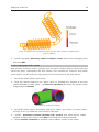
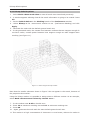
The objective of this case study is implementing a mechanical part in order to study it
through meshing analysis. The development of the model consists of the following steps:
Creating a profile of the part
Generating a volume defined by the profile
Generating the mesh for the part
At the end of this case study, you should be able to handle the 2D tools available in GiD as
well as the options for generating meshes and visualizing the prototype.
4.1 Working by layers
4.1.1 Defining the layers
A geometric representation is composed of four types of entities, namely points, lines,
surfaces, and volumes.
A layer is a grouping of entities. Defining layers in computer-aided design allows us to work
Defining the layers
44
collectively with all the entities in one layer.
The creation of a profile of the mechanical part in our case study will be carried out with the
help of auxiliary lines. Two layers will be defined in order to prevent these lines from
appearing in the final drawing. The lines that define the profile will be assigned to one of
the layers, called the "profile" layer, while the auxiliary lines will be assigned to the other
layer, called the "aux" layer. When the design of the part has been completed, the entities
in the "aux" layer will be erased.
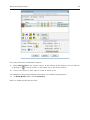
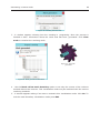
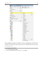
4.1.2 Creating two new layers
1 . Open the layer management window. This is found in Utilities->Layers and groups.
2 . Create two new layers called "aux" and "profile."
3 . Choose
aux
as the activated layer. From now on, all the entities created will belong
to this layer.
Figure 1. The layers window
NOTE: You can also access to the layers information through the standard bar. The layer in
use is selected in the combobox.
4.2 Creating a profile
In our case, the profile consists of various teeth. Begin by drawing one of these teeth,
which will be copied later to obtain the entire profile.
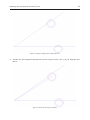
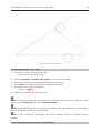
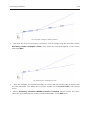
4.2.1 Creating a size-55 auxiliary line
1 . Choose the Line option, by going to Geometry->Create->Straight line or by going
1
to the GiD Toolbar .
2
2 . Enter the coordinates of the beginning and end points of the auxiliary line . For our
Creating a size-55 auxiliary line
45
example, the coordinates are (0,0) and (55,0), respectively. Besides creating a straight
line, this operation implies creating the end points of the line.
3
3 . Press ESC to indicate that the process of creating the line is finished. Press ESC again
to end the line creation function.
4 . If the entire line does not appear on the screen, use the Zoom Frame option, which is
located in the GiD toolbar and in Zoom in the mouse menu.
Figure 2. Creating a straight line
NOTE: The Undo option, located in Utilities->Undo, enables you to undo the most recent
operations. When this option is selected, a window appears in which all the operations to be
undone can be selected.
_____________________________________________________________________
1
The GiD Toolbar is a window containing the icons for the most frequently executed
operations. For information on a particular tool, click on the corresponding icon with the
right mouse button.
2
The
coordinates of a point may be entered on the command line, not enclosed in
parentheses, either with a space or a comma between them. If the Z coordinate is not
entered, it is considered 0 by default. After entering the numbers, press Return. Another
option for
entering a
point is
using the
Coordinates
Window,
found in
Utilities->Tools->Coordinates Window.
3
Pressing the ESC key is equivalent to pressing the center mouse button.
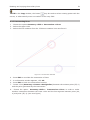
4.2.2 Dividing the auxiliary line near coordinates (40, 0)
1 . Choose Geometry->Edit->Divide->Lines->Near point. This option will divide the
line at the point ("element") on the line closest to the coordinates entered.
2 . Enter the coordinates of the point that will divide the line. In this example, the
coordinates are (40, 0). On dividing the line, a new point (entity) has been created.
3 . Select the line that is to be divided by clicking on it.
4 . Press ESC to indicate that the process of dividing the line is finished. Press ESC again
to finish the dividing function.
Figure 3. Division of the straight line near "point" (coordinates (40,0))
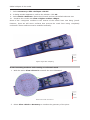
Creating a 3.8-radius circle around point (40, 0)
46
4.2.3 Creating a 3.8-radius circle around point (40, 0)
1 . Choose the option Geometry->Create->Object->Circle.
2 . The center of the circle (40, 0) is a point that already exists. To select it, go to
Contextual->Join Ctrl-a in the mouse menu (right-click). The pointer will become a
square, which means that you may click an existing point.
3 . The Enter Normal window appears. Set the normal as Positive Z and press OK.
4
4 . Enter the radius of the circle. The radius is 3.8 . Two circumferences are visualized;
the inner circumference represents the surface of the circle.
Press ESC to indicate that the process of creating the circle is finished.
Figure 4. Creating a circle around a point (40, 0)
_____________________________________________________________________
4
In GiD the decimals are entered with a point, not a comma.
4.2.4 Rotating the circle -3 degrees around a point
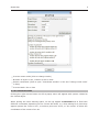
1 . Use the Move window, which is located in Utilities->Move.
2 . Within the Move menu and from among the Transformation possibilities, select
Rotation. The type of entity to receive the rotation is a surface, so from the Entities
type menu, choose Surfaces.
3 . Enter -3 in the Angle box and check the Two dimensions option. (Provided we
define positive 2D rotation in the mathematical sense, which is counter-clockwise, -3
degrees equates to a clockwise rotation of 3 degrees).
4 . Enter the point (0, 0, 0) under First Point. This is the point that defines the center of
rotation.
5 . Click Select to select the surface that is to rotate, which in this case is that of the
circle.
6 . Press ESC (or Finish in the Move window) to indicate that the selection of surfaces
to rotate has been made, thus executing the rotation.
Rotating the circle -3 degrees around a point
47
Figure 5. The move window
4.2.5 Rotating the circle 36 degrees around a point and copying it
1 . Use the Copy window, located in Utilities->Copy.
2 . Repeat the rotation process explained in section Rotating the circle -3 degrees around
a point -pag. 46-, but this time with an angle of 36 degrees.
Rotating the circle 36 degrees around a point and copying it
48
Figure 6. Result of the rotations
NOTE: The Move and Copy operations differ only in that Copy creates new entities while
Move displaces entities.
4.2.6 Rotating and copying the auxiliary lines
1 . Use the Copy window, located in Utilities->Copy.
Rotating and copying the auxiliary lines
49
Figure 7. The copy window
2 . Repeat the rotating and copying process from section for the two auxiliary lines. Select
the option Lines from the Entities type menu and enter an angle of 36 degrees.
3 . Select the lines to copy and rotate. Do this by clicking Select in the Copy window.
4 . Press ESC to indicate that the process of selecting lines is finished, thus executing the
task.
Rotating and copying the auxiliary lines
50
Figure 8. Result of copying and rotating the line
5 . Rotate the line segment that goes from the origin to point (40, 0) by 33 degrees and
copy it.
Figure 9. Result of the copy by rotation
Rotating and copying the auxiliary lines
NOTE:In the Copy window, the button
51
may be used to select existing points with the
mouse, or alternativelly enter its number in the entry field.
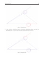
4.2.7 Intersecting lines
1 . Choose the option Geometry->Edit-> Intersection->Lines.
2 . Select the upper circle
3 . Select the line resulting from the 33-degree rotation (see next figure)
Figure 10. The two lines selected
4 . Press ESC to conclude the intersection of lines.
5 . A confirmation window appears, click Ok.
6 . Press ESC to finish the intersection function.
7 . Create a line (Geometry->Create->Straight line) between the existent point (55, 0)
and the point generated by the intersection.
8 . Choose the option
Geometry->Edit->
Intersection->Lines in order to make
another intersection between the lower circle and the line segment between point (40,
0) and point (55, 0) (see next figure)
Intersecting lines
52
Figure 11. Intersecting lines
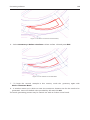
9 . Then continue selecting to make an intersection between the upper circle and the
farthest segment of the line that was rotated 36 degrees (see next figure)
Figure 12. Intersecting lines
Creating an arc tangential to two lines
53
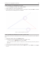
4.2.8 Creating an arc tangential to two lines
1 . Choose Geometry->Create->Arc->Fillet curves.
2 . Enter a radius of 1.35 in the command line.
3 . Now select the two line segments shown in next figure. Then press ESC to indicate
that the process of creating the arcs is finished.
Figure 13. The line segments to be selected
4.2.9 Translating the definitive lines to the "profile" layer
The auxiliary lines will be eliminated and the "profile" layer will contain only the definitive
lines.
1 . Select the "profile" layer in the Layers window.
2 . We will move the lines defining the profile to the "profile" layer:
Click on the icon
(Send To) and select Lines
Be sure that 'Also lower entities' is chequed, to send to this layer also the points of
the lines.
3 . Select only the lines that form the profile (see next figure).
4 . To conclude the selection process, press the ESC key or click Finish in the Layers
window.
Translating the definitive lines to the "profile" layer
54
Figure 14. Lines to be selected
4.2.10 Deleting the "aux" layer
1 . Select the "profile" layer and set it off.
Click on the light bulb icon
2 . Choose Geometry->Delete->All Types (or use the GiD Toolbar).
3 . Select all the lines and surfaces that appear on the screen.
4 . Press ESC to conclude the selection of elements to delete.
y and delete it.
5 . Select the "aux" layer
Click in the
icon
6 . Select the "profile" layer and set it on.
NOTE: To cancel the deletion of elements after they have been selected, open the mouse
menu, go to Contextual and choose Clear Selection.
NOTE: Elements forming part of higher level entities may not be deleted. For example, a
point that defines a line may not be deleted.
NOTE: A layer containing information may not be deleted. First the contents must be
deleted.
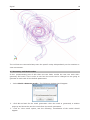
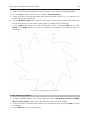
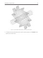
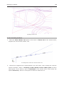
4.2.11 Rotating and obtaining the final profile
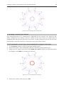
Rotating and obtaining the final profile
55
1 . Make sure that the activated layer is the "profile" layer. (Use the option To use).
2 . In the Copy window, select the line rotation (Lines,Rotation).
3 . Enter an angle of 36 degrees. Make sure that the center is point (0, 0, 0) and that you
are working in two dimensions.
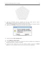
4 . In the Multiple Copies box enter 9. This way, 9 copies will be made, thus obtaining
the 10 teeth that form the profile of the model (9 copies and the original).
5 . Click Select and select the lines defining the profile. Press the ESC key or click
Finish in the Copy window in order to conclude the operation. The result is shown in
next figure.
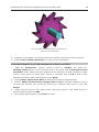
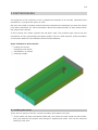
Figure 15. The part resulting from this process
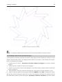
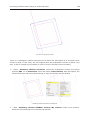
4.2.12 Creating a surface
1 . Create a NURBS surface. To do this, select the option Geometry->Create->NURBS
surface->By contour. This option can also be found in the GiD Toolbar.
2 . Select the lines that define the profile of the mechanical part and press ESC to create
the surface.
3 . Press ESC again to exit the function.
Creating a surface
56
Figure 16. Creating a surface by contour
NOTE: To create a surface there must be a set of lines that define a closed contour.
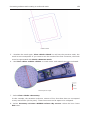
4.3 Creating a hole in the mechanical part
In the previous sections we drew the profile of the part and we created the surface. In this
section we will make a hole, an octagon with a radius of 10 units, in the surface of the part.
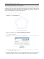
First we will draw the octagon.
1 . Select from the menu
Geometry->Create->Object->Polygon to create a regular
polygon.
2 . Enter 8 as the number of sides of the polygon.
3 . Enter (0,0,0) as the center of the polygon. (use Ctrl-a keys to swap to select new point
mode if required)
4 . Select Positive Z as the normal of the polygon, this mean a normal direction (0,0,1)
5 . Enter 10 as the radius of the polygon and press ENTER. Press ESC to finish the action.
We get the result as shown in figure 20. As we only need the boundary we should remove
the associated surface. Select the option Geometry->Delete->Surfaces and then select
Creating a hole in the mechanical part
57
the surface of the octagon. Press ESC to finish.
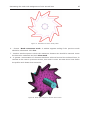
Figure 17. Regular 8-sided polygon
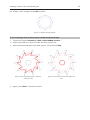
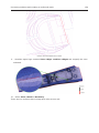
4.3.1 Creating a hole in the surface of the mechanical part
1 . Choose the option Geometry->Edit->Hole NURBS surface.
2 . Select the surface in which to make the hole (Figure 18).
3 . Select the lines that define the hole (Figure 19) and press ESC.
Figure 18. The selected surface in which to
Figure 19. The selected lines that define the
create the hole
hole
4 . Again, press ESC to exit this function.
Creating a hole in the surface of the mechanical part
58
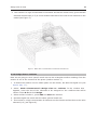
Figure 20. The model part with the hole in it
4.4 Creating volumes from surfaces
The mechanical part to be constructed is composed of two volumes: the volume of the
wheel (defined by the profile), and the volume of the axle, which is a prism with an
octagonal base that fits into the hole in the wheel. Creating this prism will be the first step
of this stage. It will be created in a new layer that we will name "prism".
4.4.1 Creating the "prism" layer and translating the octagon to this layer
1 . In the Layers window, create a new layer named "prism".
2 . Select the "prism" layer and double-click it to choose as the activated layer.
3 . Right-click on "prism" layer and select Send To->Lines. Select the lines that define
the octagon. Press ESC to conclude the selection.
Figure 21. The lines that form the octagon
4 . Select the "profile" layer and set it Off.
Creating the volume of the prism
59
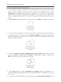
4.4.2 Creating the volume of the prism
1 . First copy the octagon a distance of -50 units relative to the surface of the wheel,
which is where the base of the prism will be located. In the Copy window, choose
Translation and Lines. Since we want to translate 50 units, enter two points that
define the vector of this translation, for example (0, 0, 0) and (0, 0, 50). (Make sure
that the Multiple Copies value is 1, since the last time the window was used its value
was 9).
2 . Choose Select and select the lines of the octagon. Press ESC to conclude the selection.
Figure 22. Selection
of the lines that
form the octagon
3 . Since the Z axis is parallel to the user's line of vision, the perspective must be changed
to visualize the result. To do this, use the Rotate Trackball tool, which is located in the
GiD Toolbox and in the mouse menu. (or press <Caps> key and drag the righ-mouse
button to rotate the view)
Figure 23. Copying the
octagon and changing the
perspective
4 . Choose Geometry->Create->NURBS surface->By contour. Select the lines that
form the displaced octagon and press ESC to conclude the selection. Again, press
ESC to exit the function of creating the surfaces.
Figure 24. The surface
created on the
translated octagon
5 . In the Copy window, choose Translation and Surfaces. Make a translation of 110
units. Enter two points that define a vector for this translation, for example (0, 0, 0) and
(0, 0, -110).
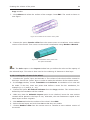
6 . To create the volume defined by the translation, select Do Extrude Volumes in the
Creating the volume of the prism
60
Copy window.
7 . Click Select and select the surface of the octagon. Press ESC. The result is shown in
next figure.
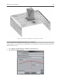
Figure 25. Creation of the volume of the prism
8 . Choose the option Render->Flat from the mouse menu to visualize a more realistic
version of the model. Then return to the normal visualization using Render->Normal.
Figure 26. Visualization of the prism with
the option RenderFlat.
NOTE: The Color option in the Layers window lets you define the color and the opacity of
the selected layer. This color is then used in the rendering of elements in that layer.
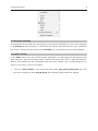
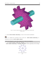
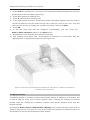
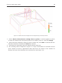
4.4.3 Creating the volume of the wheel
1 . Visualize the "profile" layer and activate it. The volume of the wheel will be created in
this layer. Set off the "prism" layer in order to make the selection of the entities easier.
2 . In the Copy window, choose Translation and Surfaces. A translation of 10 units will
be made. To do this, enter two points that define a vector for this translation, for
example (0, 0, 0) and (0, 0, -10).
3 . Choose the option Do Extrude Volumes from the Copy window. The volume that is
defined by the translation will be created.
4 . Make sure that the Maintain Layers option is not checked, hence the new entities
created will be placed in the layer to use; otherwise, the new entities are copied to the
same layers as their originals
5 . Click Select and select the surface of the wheel. Press ESC.
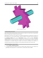
6 . Select the two layers and click them On so that they are visible.
7 . Choose Render->Flat from the mouse menu to visualize a more realistic version of
the model.
Creating the volume of the wheel
61
Figure 27. Image of the wheel
4.5 Generating the mesh
Now that the part has been drawn and the volumes created, the mesh may be generated.
First we will generate a simple mesh by default.
Depending on the form of the entity to be meshed, GiD performs an automatic correction of
the element size. This correction option, which by default is activated, may be modified in
the Meshing->Main branch of the Preferences window, under the option Automatic
correct sizes. Automatic correction is sometimes not sufficient. In such cases, it must be
indicated where a more precise mesh is needed. Thus, in this example, we will increase the
concentration of elements along the profile of the wheel by following two methods: 1)
assigning element sizes around points, and 2) assigning element sizes around lines.
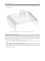
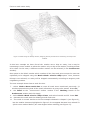
4.5.1 Generating a coarse mesh
1 . Choose Mesh->Generate mesh.
2 . A window comes up in which to enter the desired edge element size of the mesh to be
generated. Set a big size of 10 units to have a coarse mesh and click OK.
Generating a coarse mesh
62
Figure 28. Choosing elements size
3 . A window appears showing how the meshing is progressing. Once the process is
finished it show information about the mesh that has been generated. Click View
mesh to visualize the resulting mesh.
Figure 30. The mesh
generated
Figure 29. Mesh generated information
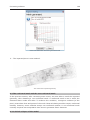
4 . Use the Mesh->View mesh boundary option to see only the contour of the volumes
meshed without the interiors. This visualization mode may be combined with the various
rendering methods.
5 . A window appears asking if we want to maintain this visualization mode. Click No. To
exit the mesh boundary visualization mode press ESC.
Generating a coarse mesh
63
Figure 31. Mesh visualized with the Mesh->View mesh boundary option
6 . Visualize the mesh generated with the various rendering options in the Render menu,
located in the mouse menu.
Generating a coarse mesh
64
Figure 32. Mesh visualized with Mesh->View mesh boundary combined with
Render->Flat.
7 . Choose View->Mode->Geometry to return to the normal visualization.
NOTE: To visualize the geometry of the model use
View->Mode->Geometry. To
visualize the mesh use View->Mode->Mesh.
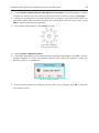
4.5.2 Generating the mesh with assignment of size around points
1 . Choose View->Rotate->Plane XY (Original). This way we will have a side view, and
View->Mode->Geometry and Render->Normal to see the geometry like the image
Figure 33. Side view of the
part.
Generating the mesh with assignment of size around points
65
2 . Choose Mesh->Unstructured->Assign sizes on points. A window appears in which
to enter the element size around the point to be selected. Enter 0.7 and click Assign.
3 . Select only the points on the wheel profile (see next figure). One way of doing this is to
select the entire part and then deselect the points that form the prism hole. Press
ESC to conclude the selection process.
4 . The window appears again, click Close to finish.
Figure 34. The selected
points of the wheel profile
5 . Choose Mesh->Generate mesh.
6 . A window opens asking if the previous mesh should be eliminated. Click Yes. Another
window appears in which the desired element size should be entered. Leave the
previous value of 10 unaltered.
Figure 35. Erasing old mesh
7 . A third window shows the meshing process. Once it has finished, click OK to visualize
the resulting mesh.
Generating the mesh with assignment of size around points
66
Figure 36. Mesh with assignment of sizes around the
points on the wheel profile
8 . A greater concentration of elements has been achieved around the points selected.
9 . Choose View->Mode->Geometry to return to this visualization.
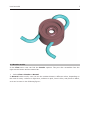
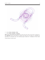
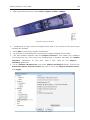
4.5.3 Generating the mesh with assignment of size around lines
1 . Open the
Preferences
window, which is found in
Utilities, and select the
Meshing->Main branch. In this window there is an option called Unstructured size
transitions which defines the size gradient of the elements. A high transition number
means a fast grown of small sizes. Select a
transition size of 0.8 to have a fast
transition and then obtain few elements. Click Apply.
2 . Choose Mesh->Reset mesh data to delete the previously assigned sizes.
3 . Choose Mesh->Unstructured->Assign sizes on lines. A window appears in which
to enter the element size around the lines to be selected. Enter size 0.7 and click
Assign.
4 . Select only the lines of the wheel profile (see next figure) in the same way as in
previous section and press ESC.
5 . The window appears again, click Close to finish.
Generating the mesh with assignment of size around lines
67
Figure 37. Selected lines of the wheel profile
6 . Choose
Mesh->Generate mesh. A window appears asking if the previous mesh
should be eliminated. Click Yes.
7 . Another window opens in which the maximum element size should be entered. Leave
the last value unaltered and click View mesh.
8 . A greater concentration of elements has been achieved around the selected lines. In
contrast to the case in previous section, this mesh is more accurate since lines define
the profile much better than points do.
Figure 38. Mesh with assignment of sizes around lines
IMPLEMENTING A COOLING PIPE
68
69
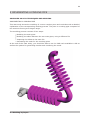
5 IMPLEMENTING A COOLING PIPE
ADVANCED 2D & 3D TECHNIQUES AND MESHING
IMPLEMENTING A COOLING PIPE
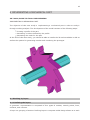
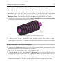
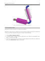
This case study shows the modeling of a more complex piece and concludes with a detailed
explanation of the corresponding meshing process. The piece is a cooling pipe composed of
two sections forming a 60-degree angle.
The modeling process consists of four steps:
Modeling the main pipes
Modeling the elbow between the two main pipes, using a different file
Importing the elbow to the main file
Generating the mesh for the resulting piece
At the end of this case study, you should be able to use the CAD tools available in GiD as
well as the options for generating meshes and visualizing the result.
5.1 Working by layers
Working by layers
70
Various auxiliary lines will be needed in order to draw the part. Since these auxiliary lines
must not appear in the final drawing, they will be in a different layer from the one used for
the finished model.
Create the layers called "part1", "union" and delete the layer "Layer0"
Choose "part1” as the activated 'layer to use'. From now on, all the entities created will
belong to this layer.
5.2 Creating a component part
In this section the entire model, except the T junction, will be created. The model to be
created is composed of two pipes forming a 60-degree angle. To start with, the first pipe
will be created. This pipe will then be rotated to create the second pipe.
5.2.1 Creating the profile
1 . Choose the Line option, located in Geometry->Create->Straight line.
2 . Enter the following new points in the command line: (0, 11), (8, 11), (8, 31), (11, 31),
(11, 11) and (15, 11). Press ESC twice to indicate that the process of creating lines is
finished.
Figure 1. Profile of one of the disks around the pipe
3 . From the Copy window, choose Lines and Translation. A translation defined by
points A (0, 11) as first point and B (15, 11) as second point will be made. In the
Multiple copies option, enter 8 (the number of copies to be added to the original). Be
sure than the 'Collapse' option is set, and then Select the lines that have just been
drawn and press ESC.
Figure 2. The profile of the disks using Multiple copies
4 . Create a line using
Geometry->Create->Straight line. Use the contextual option
Join or press <Ctrl-a> and select the last point on the profile (at the right part of the
profile). Now choose the option No join Ctrl-a and enter new point (160, 11) in the
command line. Press ESC twice to finish the process of creating lines.
5 . Again, choose the Line option and enter the new points (0, 9) and (160, 9). Press
ESC twice to conclude the process of creating lines.
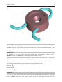
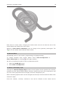
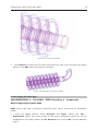
5.2.2 Creating the surfaces by revolution
Creating the surfaces by revolution
71
Rotation of the profile will be carried out in two rotations of 180 degrees each.
1 . From the Copy window, select Lines and Rotation. Enter an angle of 180 degrees
and from the Do extrude menu, select Surfaces. The axis of rotation is that defined by
the line that goes from point (0, 0) to point (200, 0). Enter these two points as the First
Point and Second Point (Two dimensions must be unchecked). Be sure to enter 2 in
Multiple copies. and select all lines and press ESC when the selection is finished.
2 . Rotate the view from the mouse menu Rotate->Trackball and choose Render->Flat
to visualize a more realistic version of the model.
Figure 3. The pipe with disks, created by rotating the profile.
3 . Return to the normal
visualization with
Render->Normal. This option is more
comfortable to work with. To return to the side view (elevation), choose in the mouse
menu Rotate->Plane XY (Original).
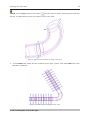
5.2.3 Creating the union of the main pipes
1 . Choose the Zoom->In option from the mouse menu. Magnify the right end of the
model and rotate the view to facilitate the selection.
2 Set "union" as current layer to use, with a <Double-click>
3 . From the Copy window, select Lines and Rotation. Enter an angle of 120 degrees
and select the rotation center (160, 25) as First point. Since the rotation may be done in
2D, choose the option Two Dimensions. From the Do extrude menu, select Surfaces
and be sure that Multiple copies is 1and Maintain layers is unset, then the new
entities will be created in the layer to use instead of the layer of the source curves.
Creating the union of the main pipes
72
Figure 4. The lines to be selected
4 . Click Select and select the four lines that define the right end of the pipe (see figure
above). Press ESC when the selection is finished.
Figure 5. Result of the extrusion by rotation
5.2.4 Copying the main pipe
IMPLEMENTING A COOLING PIPE>Creating a component
part>Copying the main pipe
Align uses a rigid body movement defined by three source points and its destination
points.
1 .
From the
Copy
window,
select
Surfaces and
Align.
Choose the
Two
Dimensions option. The source points S1, S2 and its destination points D1, D2 are
highlighted in the image. Ensure the Do Extrude menu is set to No. and set Maintain
layers.
Copying the main pipe
73
NOTE: In the Copy window, the button
may be used to select existing points with the
mouse, or alternativelly enter its number in the entry field.
Figure 6. pairs of points to define the 'Align' movement
2 . Click Select and select all the surfaces of the layer "part1" and press ESC when the
selection is finished.
Figure 7. Geometry of the two pipes and its union
5.2.5 Creating the end of the pipe
Creating the end of the pipe
74
1 . From the Copy window, select Surfaces and Rotation. Enter an angle of 180
degrees. Since the rotation may be done in 2D, choose the option Two Dimensions.
The center of rotation is the upper right point of the pipe elbow. Make sure the Do
Extrude menu is set to No.
2 . Click Select and select the surfaces that join the two pipe sections and press ESC.
3 . Select
Utilities->Move window, select Surfaces and
Translation. The points
defining the translation vector are circled in next figure.
Figure 8. The circled points define the translation vector.
4 . Click Select and select the surfaces created in point 1. Press ESC. The result should be
as is shown.
Creating the end of the pipe
75
Figure 9. The final position of the translated elbow.
5 . To create a ring surface, choose
Geometry->Create->NURBS
Surface->By
contour and select the four lines that define the opening of the pipe (see next figure).
Press ESC twice.
Figure 10. Opening at the end of the pipe
From the Files menu, choose Save in order to save the file. Enter a name for the file and
click Save.
5.3 Creating the T junction
Now, an intersection composed of two pipe sections will be created in a separate file. Then
this file will be imported to the original model to create the entire piece.
5.3.1 Creating one of the pipe sections
1 . Choose Files->New, thus starting work in a new file.
2 . Rename the layer 'Layer0' to 'pipe1' and create two new childs layers "inner" and
"outer". Set 'pipe1//inner' as layer to use with a <Double-click>
Creating one of the pipe sections
76
3 . Choose Geometry->Create->Point and enter new point (0, 9)
4 set
'pipe1//outer' as layer to use and create the new point (0, 11). Press ESC to
conclude the creation of points.
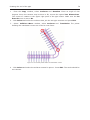
5 . From the Copy window, select Points and Rotation. Enter an angle of 180 degrees
and from the Do extrude menu, select Lines. The axis of rotation is the x axis. Enter
two points defining the axis, one in First Point and the other in Second Point, for
example, (0, 0, 0) and (1, 0, 0) , check Maintain layers, and set Multiple copies to 2.
6 . Click Select and select the two points just created. Press ESC.
Figure 11. the current model
7 . Create a surface: choose Geometry->Create->NURBS Surface->By contour and
select the four lines. Press ESC twice.
8 . From the Copy window, choose Surfaces and Translation. In First Point and
Second Point, enter the points defining the translation vector. Since the pipe section
must measure 40 length units, the vector is defined by points (0, 0, 0) and (-40, 0, 0).
9 . From the Do extrude menu, choose the Volumes option, and set Multiple copies to
1.
10 . Click Select to select the surface. Press ESC to conclude the selection process.
Figure 12. Creating a pipe by extruding the ring
5.3.2 Creating the other pipe section
1 . Create a new layer named "pipe2" with two child layers "inner" and "outer". Set
"pipe2//inner" as the 'layer to use', and set off the layers "pipe1"
2 . Choose Geometry->Create->Point and enter points (-20, 9) and (-20, 11). Press
ESC to conclude the creation of points.
3 . Change the layer of the second point to "pipe2//outer"
4 . From the Copy window, select Points and Rotation. Enter an angle of 180 degrees
and from the Do extrude menu, select Lines. Since the rotation can be done on the
xy plane, choose Two Dimensions. The center of rotation is the coordinates (-20, 0,
0), and set Multiple copies to 2
5 . Click Select and select the two points just created.
Creating the other pipe section
77
6 . Create a surface: choose Geometry->Create->NURBS Surface->By contour and
select the four lines. Press ESC twice.
7 . From the Copy window, select Surfaces and Translation. In First Point and Second
Point enter the points defining the translation vector. Since this pipe section must also
measure 40 length units, the vector is defined by points (0, 0, 0) and (0, 0, 40).
8 . From the Do extrude menu, select the Volumes option and set Multiple copies to 1.
9 . Click Select to select the surface and press ESC to conclude the selection.
Figure 13. A rendering of the two overlapping pipes
5.3.3 Creating the lines of intersection
1 . Set off the layers "outer" to facilitate the selection
2 . Choose Geometry->Edit->Intersection->Surfaces.
3 . Select the three inner surfaces of the pipes that are intersecting.
Figure 14. The inner surfaces to be intersected
4 . Repeat the process with the three outer surfaces of the pipes that are intersecting.
Now the intersection lines are created and some surfaces are splitted by these lines.
5.3.4 Deleting surfaces and close a volume
1 . Choose
Geometry->Delete->Volumes and select the two volumes, to be able to
delete some of its unwanted surfaces.
2 . Choose Geometry->Delete->Surfaces and select the small surfaces inside the first
pipe. Select Lower Entities in the contextual menu, to delete its dependencies also.
Press ESC to conclude the process of selection.
Deleting surfaces and close a volume
78
Figure 15. Surfaces to be deleted
3 . Use Geometry->Create->Volume->By contour and select all surfaces
Figure 16. The volume of a T junction
4 . From the Files menu, select Save to save the file. Enter a name for the file and click
Save.
5.4 Importing the T junction to the main file
The two parts of the model have been drawn. Now they must be joined so that the final
volume may be created and a mesh of the volume may be generated.
5.4.1 Importing a GiD file
1 . Choose Open from the Files menu. Select the file where the first part, created in
section Creating a component part -pag. 70-, was saved. Click Open.
2 . Choose Files->Import->Insert GiD model from the menu. Select the file where the
second part, created in section Creating the T junction -pag. 75-, was saved. Click
Open.
3 . The T junction appears. Bear in mind that the lines which define the end of the first
pipe (background) of the T junction, and which have been imported, were already
present in the first file. Notice that the lines are duplicated. This overlapping will be
remedied by collapsing the lines.
4 . Check duplicated lines with the tool View->Higherentities->Lines
Importing a GiD file
79
Figure 17. Importing the T junction file to the main file. Some entities are duplicated and
must be collapsed.
5 . Choose the option Geometry->Edit->Collapse->Lines. Select the overlapping lines
and press ESC.
5.4.2 Creating the final volume
Now we have a volume of the T junction, and we want to create another volume with the
rest of the piece, connected to the first volume. Two volumes are connect if they share
some surface. we will reuse the ring surface of the first volume for the new volume.
1 . Set off the layers "part1" and "union"
2 . Send the shared surface to the "part1" layer, to facilitate the selection of the new
volume boundary: select "part1", use Send to->Surfaces and select the surface of the
image and press Escape
Figure 18. Surface to be shared
3 . Set off the layers "pipe1" and "pipe2" and set on "part1" and "union", and send "part1"
as layer to use, to create the new volume in this layer.
4 . Choose
Geometry->Create->Volume->By contour and select all the visible
surfaces to define the volume. Press ESC to conclude the selection process.
5 . Choose Render->Smooth to visualize a more realistic version of the model.
Creating the final volume
80
Figure 19. A rendering of the finished piece of equipment
5.5 Generating a mesh
Now that the model is finished, it is ready to be meshed.
Generate a coarse mesh is a good test to check that the model is correct and is valid to be
used in a numerical simulation. We will use default meshing settings.
1 . Choose Mesh->Generate mesh.
2 . A window opens in which to enter the edge size of the mesh to be generated. Set a
value of 5 units and click OK.
3 . When the meshing process is finished, a window appears with information about the
mesh, press View mesh in order to be showed.
Generating a mesh
81
Figure 19. The volume mesh of tetrahedra
ASSIGNING MESH SIZES
82
83
6 ASSIGNING MESH SIZES
ASSIGNING SIZES TO THE ELEMENTS OF A MESH
The objective of this example is to mesh a mechanical piece using the various options in
GiD for assigning sizes to elements, and the different surface meshers available. In this
example a mesh is generated for each of the following methods for assigning sizes, using
different surface meshers:
Assigning sizes around points
Assigning sizes around lines
Assigning sizes on surfaces
Assigning sizes with Chordal Error
6.1 Introduction
In order to carry out this example, start by opening the project "ToMesh4.gid”. This project
contains a geometry that will be meshed using four different methods, each one resulting in
a different density of elements in certain zones.
6.1.1 Reading the initial project
1 . Open the project " ToMesh4.gid" .
2 . The geometry appears on the screen. It is a set of surfaces.
3 . Change the render mode (from the mouse menu, or from the status bar) and rotate
the model in order to get a better perception of the geometry of the model.
4 . Finally, return to the normal visualization, selecting Render->Normal. This mode is
Reading the initial project
84
more user-friendly.
Figure 1. The geometrical model of ToMesh4.gid project
6.2 Element-size assignment methods
GiD automatically corrects element sizes according to the shape of the entity to be meshed
and its
surrounding entities. This default option may be
Utilities menu, selecting
changed by going to the
Preferences, and then Automatic correct sizes
2
inside
3
Meshing branch .
Sometimes, however, this type of correction is not sufficient and it is necessary to indicate
where on the mesh greater accuracy is needed. In these cases, GiD offers various options
and methods allowing sizes to be assigned to elements.
To be sure that all the preferences are the ones used in this tutorial and get the same mesh
as result, set the default values for all the preferences:
Press
Default
values
bottom
button in the
Meshing
branch of the
Preferences window and Close the window.
_____________________________________________________________________
2
The different options are: None, no size correction is made; Normal, a size correction is
made according to the sizes of geometrical entities and the compatibility between meshing
sizes of neighboring entities; Hard, the Normal correction is made and, furthermore, an
automatic chordal error criteria is applied to assign sizes to surfaces which are the contours
Element-size assignment methods
85
of some volume in order to improve volume meshes.
3
Similar options to Automatic correct sizes but to execute them manually one time can
be found on Mesh->Untructured->Correct Sizes...
6.2.1 Assign general mesh size witth default options
To generate the mesh using the default options:
1 . Select Mesh->Generate Mesh.
2 . A window appears showing the maximum element size. This is the general mesh size
that will be used for meshing the whole model. Leave this default size unaltered and
click OK.
3 . A meshing process window opens. Then another window appears with information
about the mesh generated. Click View Mesh to visualize the mesh (see Figure 2).
Figure 2. Meshing by default
Note that in the zone highlighted in Figure 3, elements are smaller than in the rest of the
model. This is because of the shape of the surface placed there. When all meshing
preferences are set by default, as for this example, the RFAST surface mesher is used. In
this way, geometrical entities are meshed hierarchically: first of all lines are meshed, then
the surfaces, and finally the volumes. The line elements size depends on the shape of
surfaces (as can be seen in this example). Later on we will see an example using RJUMP
mesher, where element sizes are distributed differently.
Assign general mesh size witth default options
86
Figure 3. Meshing by default. Zone where elements are smaller because of the surface shape.
6.2.2 Assign size to points
1 . Select Mesh->Unstructured->Assign size on points. A window appears in which to
enter the element size around the points to be chosen. Enter 0.1 and click Assign.
2 . Select the point indicated in Figure 4. Press ESC
4
to indicate that the selection of
points is finished, and Close the window.
3 . Select Mesh->Generate Mesh.
4 . A window opens asking whether the previous mesh should be eliminated. Click Yes.
5 . GiD then asks you to enter the general maximum element size. Leave the default value
unaltered and click OK.
6 . Click View mesh in the pop up window to see the result.
Assign size to points
87
Figure 4. Geometry of the model. The point
Figure 5. The mesh with a concentration of
around which the mesh will be concentrated.
elements around the point.
7 . A concentration of elements appears around the chosen point, given the selected size
(0.1) of these elements (see Figure 5).
One can control the way the size of the elements changes from a finer to a coarser region:
8 . Go to Utilities and open Preferences window.In the Meshing branch there is the
option Unstructured Size Transitions. This option defines the transition gradient of
element sizes (size gradient), whose values are between 0 and 1. The greater the size
gradient, the greater the change in space. To test this, enter the value 0.4 and click
Accept.
9 . Again, generate the mesh (Mesh->Generate Mesh) with the same general mesh
size.
Assign size to points
88
Figure 6. Mesh with the elements concentrated around a point, with a size gradient of 0.4.
10 . The size gradient (0.4) results in a higher density around the point (see Figure 6).
11 . Now go back and enter 0.6 in Unstructured Size Transitions. This will result in a
mesh more suitable for our objectives. Click Accept.
_____________________________________________________________________
4
Instead of pressing the ESC key, the center mouse button or the mouse wheel can also
be used.
6.2.3 Assign size to lines
We are going to set an specific mesh size to some of the lines:
1 To see entity numbers select the Label option (see Labels -pag. 15-). Select all the
lines in order to see their numbers.
2 Select Mesh->Unstructured->Assign sizes on lines. In the window that appears,
enter the size of the elements around the lines that will be chosen. Enter 0.5 and click
Assign.
3 Select the lines defining the base of the prism (i.e. lines 1, 2, 3, 4 and 40).
4 Press ESC to indicate that the selection of lines is finished, and Close the window.
5 Then gnerate the mesh again with the same general mesh size as before.
Assign size to lines
89
6 This results in a high concentration of elements around the chosen lines, given that the
selected element size (0.5) is much smaller than that of the rest of the elements in the
model (see Figure 7).
Figure 7. Mesh with a concentration of elements around lines.
6.2.4 Assign size to surfaces
Now we are going to set a specific mesh size tto the triangular surface resulting from the
section of one of the vertexes of the prism (surface number 1).
1 To detect the surface one the Label option can be chosen, but also the Signal one (see
Signal -pag. 17-).
2 Select
Mesh->Unstructured->Assign sizes on surfaces. In the window that
appears, enter the size of the elements to be assigned on the surfaces that will be
chosen. Enter 0.5 and click Assign.
3 Select surface number 1, press ESC and Close the window.
4 Generate again the mesh with the same general mesh size.
5 This results in a high concentration of elements on the choosen surface due to the value
selected (0.5) (see Figure 8).
Assign size to surfaces
90
Figure 8. Mesh with a concentration of elements on a surface.
6.2.5 Assignment following chordal error criterion
In this section, an automatic size assignment is set taking into account a given maximum
allowed chordal error.
1 Select Mesh->Unstructured->Sizes by chordal error…
2 The following window appears
Figure 9. Assign sizes by chordal error window
Assignment following chordal error criterion
91
3 . Enter 0.05 as chordal error. This error is the maximum distance between the element
generated and the real object (geometry).
4 . Enter 4 as maximum meshing size.
5 . Enter 0.1 as minimum meshing size.
6 . If the right bottom button is clicked some extra information appears. We can select a
curved line and see how the mesh will look like in this line. Click on the "line" icon and
select line 34 and try to change the chordal error value. Leave it at 0.05.
7 . Press OK.
8 To see the sizes that GiD has
assigned
automatically, you can
select the
Draw->Sizes->Surfaces option in the Mesh menu.
9 Generate the mesh with the same general mesh size.
10 The resulting mesh has a high concentration of elements in curved areas. Now our
approximation is significantly improved (see Figure 10).
Figure 10. Mesh using sizes assignment by chordal error. Here there is a greater concentration of
elements in the curved zones.
6.3 Rjump mesher
The RJump mesher is a surface mesher that meshes patches of surfaces (in 3D space) and
is able to skip the inner lines of these patches when meshing. By default, the RJump
mesher skips the contact lines between surfaces (and points between lines) that are
tangent enough.
By selecting Mesh->Draw->Skip entities (Rjump), the entities that the actual mesh is
going to skip and the ones that it is not going to skip are displayed in different colors. In
this chapter we will see the properties of this mesher.
RJump default options
92
6.3.1 RJump default options
1 . Select Mesh->Reset mesh data to reset all mesh sizes introduced previously.
2 . A window appears advising that all the mesh information is going to be erased. Press
Ok.
3 . Set the Default Values in the Meshing branch of the Preferences window.
4 . Select RJump as the unstructured mesher to use
(Preferences-Meshing) and click
Apply.
5 . Generate the mesh with the default general mesh size.
6 . In the generated mesh, the contact lines between surfaces that are tangent enough do
not have nodes; contact points between lines tangent enough are also skipped when
meshing (see Figure 11).
Figure 11. Mesh using the RJump mesher.
Note that the smaller elements shown in Figure 3 do not appear in this mesh, because of
the properties this mesher.
Using the RJump mesher it is possible to assign sizes to different entities. As an example,
select Mesh->Unstructured->Sizes by chordal error….
7 . In the window enter 0.05 as chordal error.
8 . Enter 10 as maximum meshing size and 0.1 as minimum meshing size.
9 . Press OK.
10 . Again, generate the mesh with the same default general mesh size.
11 This results in a high concentration of elements in curved areas, without the nodes in
RJump default options
93
the lines and points that mesher skips. Now our approximation is significantly improved
(see Figure 12).
Figure 12. Mesh using the RJump mesher and assigning sizes by chordal error.
6.3.2 Force to mesh some entity
If there is a line or a point that the RJump mesher would usually skip, but it is required for
you to be meshed, you can specify the entity so that it is not skipped. As an example, we
will force Rjump to mesh line number 43, in order to concentrate elements around point
number 29, as it was done in section Assign size to points -pag. 86-.
1 . Select Mesh->Mesh criteria->No skip->Lines, and select line number 43. Press
ESC.
2 . Select Mesh->Draw->Skip entities (Rjump) to display the entities that will and will
not be skipped in different colors. As is shown in Figure 13, line 43 will now not be
skipped; the rest of the lines are unaffected, and RJump will either skip or mesh them
according to its criteria.
Force to mesh some entity
94
Figure 13. Entities that will be skipped and not skipped using the RJump mesher.
3 . Select Mesh->Unstructured->Assign sizes on points. A window appears in which
to enter the element size around the points to be chosen. Enter 0.1 and click Assign.
4 . Select the point indicated in Figure 4 (point number 29). Press ESC to indicate that the
selection of points is finished and Close the window.
5 . Generate the mesh again with the default general mesh size.
6 The resulting mesh is depicted in Figure 11. A high concentration of elements around
point number 29 can be appreciated. Note that there are nodes on line number 43
because we have forced RJump not to skip this line (see Figure 14).
Force to mesh some entity
95
Figure 14. Mesh using the RJump mesher, assigning sizes by chordal error and forcing an entity to be
meshed.
In this last example we have forced the mesher not to skip an entity, but it may be
interesting in some models to allow the mesher only to skip a few entities, meshing almost
all or them. In this case, a different surface mesher can be selected (in the Preferences
window).
One option is the RSurf mesher which meshes all the lines and point except the ones set
explicitally to be skipped using the Mesh->Mesh criteria->Skip option. Here, because
RJump is not selected, no entity will be skipped automatically according to tangency with
neighboring entities.
The next example shows how to work like this.
7 . Select Mesh->Reset mesh data to reset all mesh sizes introduced previously. (A
window opens advising that all the mesh information is going to be erased. Press Ok.)
8 . Set RSurf as the
unstructured surface mesher in the Meshing branck of the
Preferences window and click Apply.
9 . Select Mesh->Mesh criteria->Skip->Lines, and select lines 48 and 53. Press ESC.
10 . Generate the mesh with the default general mesh size.
11 . The result is a mesh similar to the first example obtained in chapter 2 (see Figure 2),
but the smaller elements highlighted in Figure 3 do not appear because lines 48 and 53
(which were meshed before) are now skipped when meshing (see Figure 15).
Force to mesh some entity
Figure 15. Mesh using the RSurf mesher, with some lines skipped.
96
97
7 METHODS FOR MESH GENERATION
The objective of this example is to mesh a model using the various options available in GiD
for controlling the element type in structured, semi-structured and unstructured meshes. It
also presents how to concentrate elements and control the distribution of mesh sizes.
The six methods covered are:
Generating a mesh using tetrahedral
Generating a volume mesh using spheres
Generate a mesh using circles
Generating a volume mesh using points
Generating a mesh using quadrilaterals
Generating a structured mesh on surfaces and volumes
Generating a semi-structured volume mesh
Generating a mesh using quadratic elements
7.1 Introduction
In order to carry out this example, start from the project "ToMesh3.gid". This project
contains a geometry that will be meshed using different types of elements.
7.1.1 Reading the initial project
1 . In the Files menu, select Read. Select the project "ToMesh3.gid” and click Open.
2 . The geometry appears on the screen. It is a set of surfaces and three volumes. Select
Render->Flat from the mouse menu or from the View menu. In Figure 1 shows the
Reading the initial project
98
geometrical model loaded.
3 . Rotate and make several changes in the perspective so as to get a good idea of the
geometry involved.
Figure 1. Contents of the project “ToMesh3.gid”
Finally, return to the normal
visualization
Render->Normal. This mode is more
user-friendly.
7.2 Types of mesh
Using GiD the mesh may be generated in different ways, depending on the needs of each
2
project. The two basic types of meshes are the structured
mesh and the unstructured
3
mesh. For volumes only there is one additional type, the semi-structured mesh.
For all these types of mesh a variety of elements may be used (linear ones, triangles,
quadrilaterals, circles,tetrahedra, hexahedra, prisms, spheres or points). In this tutorial you
will become familiarized with the mesh-generating combinations available in GiD.
_____________________________________________________________________
2
A structured mesh is one in which each node is connected to a constant number of
elements.
3
A semi-structured volume mesh is one in which you can distinguish a fixed structure in
one direction, i.e. there is a fixed number of divisions. However, within each division the
mesh need not be structured. This kind of mesh is only practical for topologically prismatic
volumes.
Generating the mesh by default
99
7.2.1 Generating the mesh by default
In order to get the same results we will reset the mesh options.
1 . Open the preferences window selecting Utilities->Preferences.
2 . Select the Meshing card, click on Reset and then Accept.
3 . Select Mesh->Generate mesh.
4 . A window comes up in which to enter the maximum element size for the mesh to be
generated. As default value could change from one version of GiD to another, insert 2 to
get the same results as shown in images OK.
5 . A meshing process window comes up. Then another window appears with information
about the mesh generated. Click View mesh to visualize the mesh.
6 . The result is the mesh in Figure 2. There are various surfaces and volumes. By default,
mesh generation in GiD obtains unstructured meshes of triangles on surfaces and
tetrahedra on volumes.
7 . Select Render->Flat in mouse menuto see the mesh in render mode. As is shown in
Figure 3, volume meshes are represented a little bit differently from surface meshes,
although in both cases triangles are shown. If the triangles you see are the boundary of
a volume mesh, they are shown with black edges that are thicker than surface meshes
triangles. If the triangles form a boundary volume mesh and, at the same time, a
triangle surface mesh (this can be obtained if surfaces are selected with the option
Mesh->Mesh criteria->Mesh->Surfaces), the wider edges are colored with the color
of the surface layer. Examples of these different kinds of render are shown in Figure 3.
Figure 2. Generating the mesh by default.
Generating the mesh by default
100
Figure 3. Different render styles: a) surface mesh, b) volume mesh, c) surface mesh and volume
mesh together (surface layer is red and volume layer is blue)
7.2.2 Generating the mesh using circles and spheres
1 . Select Mesh->Element type->Sphere. Select volume number 1 and press ESC. To
see entity numbers select Label from the mouse menu or from the View menu. If you
wish the geometrical entity labels to be displayed, the view mode needs to be changed
to Geometry using View->Mode->Geometry (this option may also be found in the GiD
Toolbar). Select Render->Normal in the mouse menu to see the labels.
2 . Select Mesh->Element type->Circle. Select surface number 24 and press ESC.
3 . Select Mesh->Generate mesh.
4 . A window comes up asking whether the previous mesh should be eliminated. Click
Yes.
5 . Another window appears in which to enter the maximum element size. Leave the
default value unaltered and click OK. The result is a mesh as illustrated in Figure 4.
Generating the mesh using circles and spheres
101
Figure 4.(Render Flat) Generating a mesh on
a volume using points.
Figure 4.(Render Normal) Generating a
mesh on a volume using points.
7.2.3 Generating the mesh using points
1 . Select Mesh->Element type->Only points. Select volume number 1 and press ESC.
2 . Select Mesh->Generate mesh.
3 . A window comes up asking whether the previous mesh should be eliminated. Click
Yes.
4 . Another window appears in which to enter the maximum element size. Leave the
default value unaltered and click OK. The result is a mesh as illustrated in Figure 5.
Generating the mesh using points
102
Figure 5. Generating a mesh on a volume using points.
5 . Now volume number 1 is meshed using only the generated nodes.
7.2.4 Generating the mesh using quadrilaterals
1 . Select Mesh->Element type->Quadrilateral. Select surfaces number 24 and 12 and
press ESC.
2 . Select Mesh->Generate mesh.
3 . A window comes up asking whether the previous mesh should be eliminated. Click
Yes.
4 . Another window appears in which the maximum element size can be entered. Leave
the default value unaltered and click OK. The result will be the mesh illustrated in Figure
6.
Generating the mesh using quadrilaterals
103
Figure 6. An unstructured mesh generated using quadrilaterals.
5 . The surface is meshed with quadrilaterals, forming an unstructured mesh, surface 12
seems structured but if you zoom in, you will see that it is not.
7.2.5 Generating a structured mesh (surfaces)
1 . To mesh surfaces with a structured mesh, select the option
Mesh->Structured->Surfaces->Assign number of cells.
2 . Select all top surfaces 9, 24, 26 and 12 and press ESC.
3 . A window appears in which to enter the number of divisions that the lines to be
selected will have. Enter 4.
5
4 . Click Assign and select one vertical line (parallel to the Y axis). Press ESC.
5 . Another window appears in which to enter the number of divisions on the lines. Enter
6.
5
6 . Click Assign and select the 4 bottom lines . Press ESC.
7 . Another window appears in which to enter the number of divisions on the lines. In this
case, all the boundary lines have already been defined. Therefore, click Close.
8 . Select Mesh->Element type->Triangle. Select surfaces 26 and 12. Press ESC.
Generating a structured mesh (surfaces)
104
Figure 7. Structured mesh of quadrilateral and triangular elements on surfaces.
9 . Select Mesh->Generate mesh.
10 . A window comes up asking whether the previous mesh sould be eliminated. Click Yes.
11 . Another window appears in wihich to enter the maximum element size. Leave the
default value unaltered an click OK. The result is the mesh shown in Figure 8.
12 . As seen in Figures 7 and 8, GID can obtain surface structured meshes made of
quadrilaterals or triangles. There are tow kinds of structured mesh that use triangles:
the one shown in Figure 7 is obtained when the
Utilities->Preferences->Meshing->Main->Structured
Mesher->Symmetrical
structured->triangles option is set. If this option is not set, the mesh presented in
Figure 8 is produced (with fewer nodes than if using the previous option).
Generating a structured mesh (surfaces)
105
Figure 8. Structured mesh of quadrilateral and triangular elements on surfaces, with the option
Symmetrical structured triangles not set.
_____________________________________________________________________
5
When selecting a line, GID automatically selects all lines parallel to it.
7.2.6 Generating structured meshes (volumes)
1 . To mesh volumes with a structured mesh, select the option
Mesh->Structured->Volumes->Assign number of cells.
2 . Select volumes 1 and 2 and press ESC.
3 . A window appears in which to enter the number of divisions that the lines to be
selected will have. Enter 6 and click Assign.
4 . Select lines of both volumes parallel to the X and Z axes. GiD automatically selects all
the lines in each volume parallel to these in order to create the structured mesh. Press
ESC.
5 . Another window appears in which to enter the number of divisions on the lines. Divide
the lines parallel to the Y axis into 8 segments. Enter 8 and click Assign.
6 . Select an edge of volume 1 or 2 parallel to the Y axis and press ESC . Again, the
line-division window comes up. Since we have already finished the assignments, click
Close.
Generating structured meshes (volumes)
106
Figure 9. Structured volume mesh of hexahedra an tetrahedra.
7 . For structured volumes, GiD generates tetrahedron meshes by default, but hexahedron
structured meshes can also be assigned. Let's assign the element type that we wish to
volume 1 and 2. Select
Mesh->Element
type->Tetrahedra,then select volume
number 2 and press ESC. Select Mesh->Element
type->Hexahedra, then select
volume number 1 and press ESC.
8 . Select Mesh->Generate mesh.
9 . A window appears asking whether the previous mesh should be eliminated. Click Yes.
10 . Another window comes up in which to enter the maximum element size. Leave the
default value unaltered and click OK . The result is the mesh shown in Figure 10.
11 . GiD can obtain volume structured meshes made of hexahedra, tetrahedra or prisms.
As can be seen in Figures 9 and 10, there are two kinds of tetrahedron structured
mesh: the one shown in Figure 9 is obtained when the option
Utilities->Preferences->Meshing->Symmetrical structured->tetrahedra is set.
If this option is not set, the mesh presented in Figure 10 is produced (with fewer nodes
than if using the previous option;also, it is not topologically symmetrical).
Generating structured meshes (volumes)
107
Figure 10. Structured volume mesh of tetrahedra with the option Symmetrical structured tetrahedra
not set.
7.2.7 Generating semi-structured meshes (volumes)
1 . To
mesh
volumes
with a
semi-structured
mesh,
select
the
option
Mesh->SemiStructured->Volumes.
2 . A window appears in which to enter the number of divisions for the direction in which it
is structured (the prismatic one). Enter 8 and click Assign.
3 . Select volume 3 and press ESC. As volume 3 is prismatic in one direction only (i.e.
parallel to Y axis) GiD will automatically detect this fact and will select it to be the
direction in which the semi-structured volume mesh is structured.
4 . Another window appears in which to enter the number of divisions in the direction of
the structure. In this case we do not want to select any more volumes, so click Close.
5 . Select Mesh->Generate mesh.
6 . A window appears asking whether the previous mesh should be eliminated. Click Yes.
7 . Another window appears in which to enter the maximum element size. Leave the
default value unaltered and click OK. The result is the mesh shown in Figure 11.
Generating semi-structured meshes (volumes)
108
Figure 11. Semi-structured volume mesh of tetrahedra.
As can be seen, volume 3 has been meshed with tetrahedra. Semi-structured volumes are
meshed with prisms, by default. However, in this case it was not possible because of
volume 2, which has tetrahedra assigned and shares one surface with volume 3. In the
following steps a hexahedron mesh is produced.
8 . Select Mesh->Element type->Hexahedra.
9 . Select volumes 2 and 3 and press ESC.
10 . Select Mesh->Generate mesh.
11 . A window opens asking whether the previous mesh should be eliminated. Click Yes.
12 . Another window appears in which to enter the maximum element size. Leave the
default value unaltered and click OK. The result is the mesh shown in Figure 12.
Generating semi-structured meshes (volumes)
109
Figure 12. Semi-structured volume mesh of hexahedra.
In case of volume number 3 there is only one direction in which it can possibly be
structured (i.e. in the direction of the prism). If the volume is prismatic in more than one
direction, there are two ways to choose
between them:
selecting one top surface
(Mesh->SemiStructured->Set->Master
surface) or the
direction of the
structure
(Mesh->SemiStructured->Set->Structured direction). The following example explains
this procedure.
13 . Select the option Mesh->SemiStructured->Volumes.
14 . A window opens in which to enter the number of divisions in the structured direction
(prismatic). Enter 6.
15 . Select volume 1 and press ESC.
16 . Another window appears, click Close.
17 . Select Mesh->SemiStructured->Set->Structured direction.
18 . Select one line parallel to the X axis of volume number 1 (for example line number
11) and press ESC.
19 . Select Mesh->Unstructured->Assign entities->Surfaces.
20 . Select surfaces 1 and 6 and press ESC.
21 . Select Mesh->Generate mesh.
22 . A window opens asking whether the previous mesh should be eliminated. Click Yes.
23 . Another window appears in which to enter the maximum element size. Leave the
default value unaltered and click OK.
7.2.8 Concentrating elements and assigning sizes
1 . Select Mesh->Structured->Lines->Concentrate elements.
Concentrating elements and assigning sizes
110
2 . Select some structured lines, for example line 43. Press ESC.
3 . A window comes up in which to enter two values for the concentration of elements.
Positive values concentrate the elements and negative values spread them. Enter 0.5 as
Start Weight and –0.5 as End Weight
10
. Click Ok and press ESC.
4 . Select Mesh->Generate mesh.
5 . A window opens asking whether the previous mesh should be eliminated. Click Yes.
6 . Another window appears in which to enter the maximum element size. Leave the
default value unaltered. The result is the mesh shown in Figure 13.
Figure 13. Concentration of elements on line 43.
It is also possible to assign sizes to geometrical entities, so that mesh elements can be
concentrated in certain zones. In the following steps some examples are given.
7 . Select Mesh->Unstructured->Assign sizes on points.
8 . A window appears in which to enter the size to be assigned to points. Enter 0.1 and
click Assign.
9 . Select point number 15 and press ESC.
10 . Another window appears in which to enter the size to be assigned to points. In this
case, we donot want to assign sizes to any other points, so click Close.
11 . Select Mesh->Unstructured->Assign sizes on lines.
12 . A window appears in which to enter the size to be assigned to lines. Enter 0.5 and
click Assign.
13 . Select line number 25 and press ESC.
14 . Another window appears in which to enter the size to be assigned to lines. In this
case, we do not want to assign sizes to any more lines, so click Close.
15 . Select Mesh->Generate mesh.
Concentrating elements and assigning sizes
111
16 . A window appears asking whether the previous mesh should be eliminated. Click Yes.
17 . Another window appears in which the maximum element size should be entered.
Leave the default value unaltered and click OK. The result is not the desired, we just
get the previous mesh. This is because surrounding surfaces and lines are structured,
so they do not have enough freedom to achive the given sizes.
18 . Select Mesh->Unstructured->Assign entities->Surfaces.
19 . Select Surfaces 26 and 12. Press ESC.
20 . Select Mesh->Unstructured->Assign entities->Lines.
21 . Select lines 48, 26 and 27. Press ESC.
22 . Select Mesh->Generate mesh.
23 . A window appears asking whether the previous mesh should be eliminated. Click Yes.
24 . Another window appears in which the maximum element size should be entered.
Leave the default value unaltered and click OK. The result is the mesh shown in Figure
14.
Figure 14. Unstructured size assigned in a point and a line.
_____________________________________________________________________
10
Start Weight and End Weight refer to the start point and end point of the line, oriented
as it is drawn when you select it.
7.2.9 Generating the mesh using quadratic elements
Enlarge one area of the mesh with the zoom.
Generating the mesh using quadratic elements
112
1 . Select Label->All in->Points . The result is shown in Figure 15.
Figure 15. Each number identifies a node. There is a node for each element vertex.
2 . The node identifiers created by generating the mesh appear on the screen. There is
one identifier for each vertex of each element.
3 . Select Mesh->Quadratic type->Quadratic.
NOTE : By default GiD meshes with first degree (linear) elements. To find out which mode
GiD is working in, go to Mesh->Quadratic type.
4 . Select Mesh->Generate mesh.
5 . A window opens asking whether the previous mesh should be eliminated. Click Yes.
6 . Another window appears in which the maximum element size should be entered. Leave
the default value unaltered and click OK.
7 . Once the mesh has been generated, select Label->All in->Points . The result is
shown in Figure 16. Now, there are not only nodes at the vertices, but also at the
midpoints of the edges of the elements.
Generating the mesh using quadratic elements
113
Figure 16. Each number identifies a node. There is a node at each element vertex and at
the midpoint of each edge.
8 . Select Mesh->Quadratic type->Quadratic9.
9 . Select Mesh->Generate mesh.
10 . A window opens asking whether the previous mesh should be eliminated. Click Yes.
11 . Another window appears in which the maximum element size should be entered.
Leave the default value unaltered and click OK.
12 . Select Label->All in->Points (see Figure 17).
13 . Notice that the four-sided elements (quadrilaterals) also have a node in the center, in
addition to the nodes at the vertices and midpoints of the edges. Similarly, hexahedra
also have a node at their center point.
Figure 17. Each number identifies a node. There is a node at each vertex, at the midpoint of each
edge and in the center of quadrilaterals and hexahedra.
POSTPROCESSING
114
115
8 POSTPROCESSING
The objective of this tutorial is to do a postprocess analysis of an already calculated fluid
simulations, no preprocess option is used.
Not only the model is already meshed and the constraints are assigned, but also the results
have been calculated. For more information about the preprocess part of GiD, please check
the preprocess tutorials.
In this tutorial, the model Cylinder.bin has been used. The problem type used to do this
simulations is Tdyn, particularly the Ransol model. Tdyn is a fluid dynamic (CFD) simulation
environment based on the stabilized Finite Element Method.
Steps followed in this tutorial:
Loading the model
Changing mesh styles
Visualization of results
Creating images
8.1 Loading the model
There are two ways to load the results simulation information into GiD:
If the model has been calculated inside GiD, the results are also inside the GiD model,
then just load the GiD project and change to postprocess mode. This can be achieved
clicking on this icon:
Loading the model
116
, or selecting the Files->Postprocess menu entry.
If only a mesh and results file(s) are present then GiD should be started, and switched
to postprocess mode (
) before loading the file(s).
For this tutorial we will use the file called "Cylinder.bin" that contains the postprocess
information, so the steps to follow are:
1 . Start GiD
2 . Switch to postprocess mode:
or Files->Postprocess
3 . Open the model with: Files->Open, Ctrl-o or clicking on
8.2 Changing mesh styles
1 . Select Window->View style...
2 . Select all the layers
3 . change the style to Boundaries
4 . Play a little with the options of these windows, but to continue the tutorial, let a
Boundaries style selected for all meshes
5 . Change render mode to Normal
Changing mesh styles
117
8.3 Viewing the results
In the example, several results have been calculated for several time steps. You can check
these results through the Results menu, opening the View Results window or through the
results view icon bar.
Menu: View Results
Window->View Results...
Viewing the results
Results view icon bar:
118
Iso surfaces
119
8.3.1 Iso surfaces
Menu: View results->Iso Surfaces
With this result visualization a surface, or line, is drawn passing through all the points
which have the same result's value inside a volume mesh, or surface mesh. To create
isosurfaces there are several options.
1 . Select View results->Iso Surfaces->Automatic
Width->Velocity(m/s)->|V|throught the menu bar or clicking on
on the results
view icon bar.
After choosing the result, you are asked for a width. This width is used to create as many
isosurfaces as are needed between the Minimum and Maximum defined values (these are
included).
2 . enter the value 0.25727 to get the picture below.
3 . Select View->Render->Smooth in order to get a better view.
Several configuration options can be set via the Options menu.
Menu: Options->Iso surfaces
Using Options -> Iso surfaces -> Display Style the style of the iso-surface can also be
changed as with the volume and surface meshes.
In order to see the inner zones we will set the transpacency on the iso surfaces.
4 . Select Options->Iso Surfaces->Transparency->Transparent
5 . Move the model to see the inner zones
6 . Select Options->Iso Surfaces->Transparency->Opaque
Other interesting options are:
Iso surfaces
120
Options->Iso surfaces->Convert to cuts which consolidates the isosurface as mesh
which can be exported to a file.
Options->Iso surfaces->Color Mode allows to draw the iso-surfaces with a single
colour ( Monochrome), according to the results used to create the iso-surface ( Result
color) or using the color map of the visualized contour fill result ( Contour fill color).
Options->Iso surfaces->Show isolines this option allows the user to switch isolines
of surafaces on or off.
Options->Iso surfaces->Draw always if this option is selected the iso-surfaces are
always drawn even though all the meshes are switched off.
8.3.2 Animate
Menu:Window->Animate...
This window allows the user to animate the current visualized results.
If only one step is present, then the Static analysis animation profile button is enabled
so that a custom animation profile can be step to animate that one step.
If one result has several steps you can visualize them in an animation. In this case we will
Animate
121
use the iso surfaces result.
1 . Select View->Render->Smooth
2 . Select Window->Animate...to open the animation window
Please notice that we have from step 1 to 13. We will do the animation only of some of
these steps.
3 . Check the From step option and set 3 to step 8
4 . Select the Delay between steps option and set it to 800 ms. The animation should
take 4 seconds
5 . Try it clicking on the play icon
We will record a video during the animation.
6 . Once the animation is finished check the Save option on the Save animation part
You can choose from several video formats.
7 . Select AVI/mjpeg
(to include this animation in a MS PowertPoint an apropiate codec is needed like the one
supplied with Combined Community Codec Pack, CCCP)
8 . Select a folder where the video will be saved clicking on the folder icon or writing the
path in the text entry
9 . Click on the play button and the recording will begin. This step could take a little bit
long. Wait until the red circle turns to green
10 . Close the Animate window
Now we will visualize another result but before we will clear all the results.
11 . Select View results->No results through the menu bar or using the icon
8.3.3 Result surface
Another result visualization of interest is this one:
Result surface
122
To get this visualization follow these steps:
1 . Switch off all the sets except S interior cil. To do this:
Select Window->View style... in the menu bar.
Select all the sets except S interior cil pressing Ctrl while selecting with mouse.
Click on the bulb light icon on the I/O column or click on the icon
.
2 . Through the "View style" window change the Style to Body Bound.
3 . Select View results->Result surface-> Pressure (Pa). A surface will be drawn
which results from moving the nodes along its smoothed normal according to the results
value for this node.
4 . Enter 5 as factor in the bottom command line.
5 . Select Options->Result surface->Show elevations->None .
6 . Select Options->Result surface->Show elevations->Contour fill. With this last
option the surface is colored according to the pressure value.
Play with the other options as you will.
Result surface
123
7 . Select View results->No results through the menu bar or using the icon
8 . Switch on all the sets again through the "View style" window by selecting all sets and
clicking on the
icon.
8.3.4 Contour fill, cuts and limits
Contour fill
Menu: View results->Contour Fill
1 . Please select View results->Contour Fill->Pressure (Pa) through the menu bar, or
clicking on
or using the Window->View results... window.
2 If not all sets show the contour fill like the picture above,
remember to select
BodyBoundary mesh style for all the sets.
This option allows the visualization of coloured zones, in which a scalar variable or a
component of a vector varies between two defined values. GiD can use as many colours as
permitted by the graphical capabilities of the computer The number of colours can be set
through
Options->Contour->Number of colours. A menu of the variables to be
represented will be shown, and the one that is chosen will be displayed using the default
analysis and step selected.
In the model the pressure has been calculated. We can visualize the result for each step in
a contour fill.
You can choose the step that you want to view through the View results window or
clicking on
3 . Select the step 103
Several configuration options can be set via the Options menu.
Contour fill, cuts and limits
124
Menu: Options->Contour
You can change the color scale in orther to get a more comfortable view. You can select
several predefined color scales. The default scale is standard, which is a rainbow colour
map starting from blue (minimum) through green and yellow, to red (maximum).
1 . Select Options->Contour->Color Scale->Inverse Standard
You can also define your own scale.
2 .
Select
Options->Contour->Color
scale->User
defined... or
Options->Contour->Color Window...
In this window you can change the number of diferent colors used in the scale. If you need
more accuracy you can increase this number, or decrease it for a higher contrast.
3 . Change the number of colors to 10
4 . Click on Apply button
5 . Click on Close button
Cuts
In order to view the inner zone we will do several cuts along the model.
Contour fill, cuts and limits
125
Menu: Do cuts
In order to make it easier first we will change the plane visualization.
1 . Please select
View->Rotate->Plane
XY(Original)
through the menu bar,
and
Rotate->Plane XY(Original) throught the mouse menu or clicking on
.
Now you have a top view of the model.
2 . Select Do cuts->Cut
plane->Succession through the menu bar or clicking on
and then
With the succession option you specify an axis that will be used to create cut planes
orthogonal to this axis. The number of planes is also asked for.
3 . Draw a line through the X axis in the middle of the model and ask for 7 cuts. You
should obtain 7 parallel planes to Y axis.
Note: after clicking the first point, pressing the Alt key while moving the mouse the
dynamic line will be axis aligned or at 45 degrees.
4 . Now change the display style (Utillities->View style) in order to see only the cuts.
You can see that several layers have appeared a prefix like CCutSetX indicating which
mesh or set has been cut. These names can always be
changed
through the
Window->View Style. Select all the layers except the cuts and change their style to
Boundaries. You can rotate the model in order to see the contour fill result on the cut
planes.
5 . In the same window select all the CCutSetX and click on Delete button in order to
delete all the cuts.
6 . Select BodyBoundary as mesh style to visualize the contour fill of pressure again.
7 . Select Options->Contour->Reset all in order to set all the defaults options.
Contour fill, cuts and limits
126
Define limits
You can set the limit values for the contour fill. In our case we only want to see the positive
values. In order to do this we will set the minimum value to 0.
1 . Select Options->Contour->Define Limits... through the menu bar or clicking on
Choosing the first option the Contour Limits window appears. With this window you can set
the minimum/maximum value that Contour Fill should use.
2 . Check the Min checkbox
3 . Change the value to 0
4 . Click on the Apply button
5 . Click on the Close button
Outliers will be drawn in the colour defined in the Out Min Colour option. In order to view it
better we will change this color to transparent.
6 . Select Options->Contour->Min Options->Out Min Color->Transparent
8.3.5 Combined results
An interesting postprocess options is to combine several result visualizations, like this one:
Combined results
127
To get this view follow these steps:
1 . Clear all results visualizations with View Results->No results or the icon
2 . Select Window->Several results. Then following window appears:
3 . In this window select one over another. With this option GiD is told to visualize one
result over another
4 . Select View Results->Default Analysis/Step->Ransol->103
5 . Select View Results->Iso surfaces->Exact->Pressure through the menu bar or
clicking on the
6 . In the following questions: How many isosurfaces? Enter 1
7 . Enter the 1 value ...? Enter 0
8 . Select View Results->Contour Fill->Pressure
9 . Set the minimum value to 0
10 . Select Options->Contour->Min options->Out min color->Transparent
11 . Select Options->Contour->Color scale->Terrain Map
12 . Select Options->Iso surface -> Color mode -> Monochrome
13 . Select
Options->Iso surface -> Change color to change the color of the iso
Combined results
128
surface.
Note: On newer version of GiD, step 2 and step 3 is not needed.
8.3.6 Stereo mode (3D)
Menu: View->Advanced viewing settings...
If you have an anaglyphic glasses you can try this option. The model can be set as an
anaglyphic image in order to provide a stereoscopic 3D effect, when viewed with 2 color
glasses (each lens a chromatically opposite color, usually red and cyan).
Anaglyphic images are made up of two color layers, superimposed. Since the glasses act as
red and cyan filters we should be careful with the model's colors. To avoid problmes we will
change the contour fill color scale.
1 . Select Options->Contour->Color Scale->3D Anaglyphs
2 . Select View->Advanced viewing settings...
3 . Check the Use stereo option
Stereo mode (3D)
129
4 . Check the Dynamic update option in order to change the options without the need to
click the Apply button
5 . Set the eye distance to the value where you can see the 3D effect
6 . Unheck the Use stereo option
7 . Close the window
8 . Select View results->No Results
9 . Change the view style to boundaries for all the layers, like in Changing style chapter
8.3.7 Show Min Max
Menu: View results->Show Min Max
With this option you can see the minimum and maximum value of the chosen result in the
chosen analysis step. In our case we will choose the Vy component of velocity result for the
first analysis step.
1 . Select View results->Default Analysis/Step->RANSOL->91.5 throught the menu
bar or clicking on
2 . Select View results->Show both->Velocity (m/s)->Vy throught the menu bar or
clicking on
. The label shows the node number and the value of the result.
3 . Select View results->No Results
Show Min Max
130
8.3.8 Stream lines
Menu: View results->Stream Lines
With this option you can display a stream line, or in fluid dynamics, a particle tracing, in a
vector field.
Note: stream lines are confined in a single volume mesh, i.e. they do not jump from one
Stream lines
131
volume mesh to the next volume mesh, even if they are close neighbours. In the provided
example there are three volume meshes and stream lines will not cross the volume
boundaries. You can join the volume meshes into a single volume mesh using Utilities -->
Join --> Volume sets . Then you can delete the three separate volumes and switch the
single joined volume mesh on.
The above image results from doing this tutorial with the three separated volumes.
The image at the end of this stream lines tutorial is achieved if following step is done before
the enumerated stream lines tutorial steps.
Select Utilities --> Join --> Volume sets to create a single volume mesh, and delete
the three other volume meshes: V volumes, V cil and V wake. ( The above image results
from
1 . Select View results->Default
Analysis/Step->RANSOL->103.0 throught the
menu bar or clicking on
2 . Select View results->Stream Lines->Along line->Velocity (m/s) throught the
menu bar
With this option you can define a segment along which several start points will be chosen.
The number of points will also be asked for, including the ends of the segment. In the case
of just one start point, this will be the center of the segment.
NOTE: This action could also be done clicking on
in the icon bar. In this case we have to
select the way to define the start point through the mouse menu. In this case select
Contextual->Along line.
We want to create several stream lines along the model doing 2 lines.
3 . Write the initial point in the command line 10 15 3
4 . Write the final point in the command line 10 -15 3
5 . You are asked for the number of points along the line. Enter 5 and click Ok.
Note: (You can also press Ctrl-t to set the cursor in the command line)
The first line with 5 stream lines is created.
6 . Write the initial point in the command line 10 15 7
7 . Write the final point in the command line 10 -15 7
8 . You are asked for the number of points along the line. Choose 3.
The second line with 3 stream lines is created.
9 . Click the middle mouse button or press the Esc key in order to finish the operation.
Stream lines
132
Several configuration options can be set via the Options menu.
Menu: Options->Stream lines
The options can be also managed through the Size & detail window.
10 . Select Options->Contour->Color Scale->Standard
11 . Select Options->Stream lines->Size & detail...
12 . Check the Dynamic update option
13 . Select Stream contour filled
The stream lines will be drawn with the colors used in the velocity contour fill.
14 . In the Arrows options, set 30 for the Size option
15 . Set 10 for the Spacing option
16 . Check the Show Arrows option
17 . You may play with the diferent stream types: points, ribbons or 4 sided prisms. If the
ribbons type is selected you may adjust the initial swirl to rotate the ribbon.
18 . Close the window
19 . Select Options->Stream lines->Delete all
NOTE: A way to achive the best results is to first create a cut of the volume mesh throught
the region of interest and then use these nodal information as support to create stream
lines and its options: along line, in a quad, etc.
Stream lines
133
8.3.9 Graphs
Menu: View results->Graphs
From this menu several graphs types can be created, we will try some of them. Graphs are
supported for results defined over nodes.
Graphs are organized into graph sets in order to ease the management. Each set shares
the same units for each axis.
When a graph is created is placed in the current graphset if the units are the same,
otherwise a new graphset is created.
In order to work with graphs we will use the 'graphs window'.
The Point evolution graph displays a graph of the evolution of the selected result along all
the steps, of the default analysis, for the selected nodes.
1 . Select View results->Graphs->Point evolution->Velocity(m/s)->|V|
2 . Write 20 0 4 in the command line in order to specify the point.
3 . Affter pressing the Escape key, or the middle mouse button, the graph will be shown
in a separate window:
Graphs
134
The graph is created in the graphset-1. We will create another graph in the same graph
set.
The Line graph displays a graph defined by the line conectig two selected nodes of
surfaces or volumes, or any arbitrary points on any projectable surface and in any position.
4 . Switch all surface meshes off, and let only the three volume meshes on: V volumes, V
cil, V wake.
5 . Select View results->Graphs->Line graph->Velocity(m/s)->|V|
6 . Write 3 0 4 in the command line in order to specify the initial point.
7 . Write 50 0 4 in the command line in order to specify the final point.
Now both graphs are showed in the same graph set:
Graphs
135
We will rename the graph set.
8 . In the top part of the window click the
icon.
9 . A window will appear asking for a new name. Enter 'Velocity', for example.
We will create a new graph set.
10 . In the top part of the window click the
icon.
A new graph set is created with default name 'graphset-1'. When a new graph set is
created becomes the current one. We can see that there are no graphs on this new graph
set.
It's also possible to create graphs from the graph window.
11 . Go to Create tab and select Point evolution int View option.
12 . In Y Axis list double click Pressure (Pa).
13 . Write 50 0 0 in the command line in order to specify the point.
14 . Press Escape to finish the graph.
We can manage graphs and graphs sets in the Options panel. Depending if we are selecting
a graph set or a graph in the tree we will see different options in the tab.
15 . Go to the Options panel, select the 'Velocity (m/s) evolution at ( 20, 0, 4)' graph and
delete it pressing the button with the red cross.
16 . A confirmation window appears. Click Yes.
Graphs
136
17 . Please notice that the current graph set have been changed to 'Velocity'. Now the Plot
graph panel will show only one graph:
Graphs
137
The graph size is readapted. We can will change several style options of a graph.
18 . Double click in any point of the graph and we will access to the Options tab.
19 . Choose Line in the Style option
20 . Set to red the Color option. You can do it writing #ff0000 or selecting the red clicking
on the right color window
21 . Set to 4.0 the Line width
22 . Click on Apply button
Graph sets options can be managed selecting the set in the tree.
23 . Select 'Velocity' branch. The options will change.
24 . For instance mark 'Logarithmic scale' option in X axis.
25 . Click on Apply button
We can export the graph information in order to open it later with GiD.
26 . Select Files->Export->Graph->All. You are asked for the location where to save the
.grf file.
27 . Choose the location
Now you can import the selecting Files->Import->Graph
28 . Select Options->Graphs->Clear graphs in order to delete all the graphs
8.4 Creating images
Menu:Files->Page and capture settings...
Creating images
138
Finally we will take some snapshots of our model. You can save images in several formats.
The properties of the image (resolution, size, etc.) can be assigned in Page and capture
settings option.
1 . Select Files->Page and capture settings...
2 . Check the Auto crop image option in order to cut the image in the model limits
3 . Click on Set Page button
4 . Click on Close button
Menu:Files->Print to file
This option asks you for a file name and saves an image in the required format with the
defined properties in Page and capture settings.
1 . Select Files->Print to file->PNG... throught the menu bar
2 . Choose the location where you want to save the image
3 . Choose a name for the file
4 . Click on Save button
Creating images
NOTE: This action could also be done by clicking on
139
throught the icon bar. This icon can
also be found in the "Page and capture settings" window. In this case the image format is
choosen while saving the file in the "Files of type" combobox.
CAD CLEANING OPERATIONS
140
141
9 CAD CLEANING OPERATIONS
IMPORTING FILES
The objective of this case study is to see how GiD imports files created with other
programs. The imported geometry may contain imperfections that must be corrected
before generating the mesh.
For this study an IGES formatted geometry representing a stamping die is imported. These
steps are followed:
Importing an IGES-formatted file to GiD
Correcting errors in the imported geometry and generating the mesh
Generating a conformal mesh and a non-conformal mesh
Pice provided by courtesy of PSA DEGAD-MAC AIE
9.1 Importing on GiD
GiD is designed to import a variety of file formats. Among them are standard formats such
as IGES, DXF, or VDA, which are generated by most CAD programs. GiD can also import
meshes generated by other programs, e.g. in NASTRAN or STL formats.
Importing on GiD
The file importing process is not always
142
error-free.
Sometimes the original file has
incompatibilities with the format required by GiD. These incompatibilities must be overcome
manually. This example deals with various solutions to the difficulties that may arise during
the importing process.
9.1.1 Importing an IGES file
1 . Select Files->Import->IGES …
2 . Select the IGES-formatted file "base.igs” and click Open.
Importing an IGES file
143
Reading the file
Repairing the model
Importing process information
After the importing process, the IGES file that GiD has imported appears on the screen.
File “base.igs” imported by GiD.
Importing an IGES file
144
NOTE: One of the operations in the importing process is repairing and collapsing the
model. We say that two entities collapse when, the distance between them being less than
the Import Tolerance, they become one.
The Import Tolerance value may be modified by going to the Utilities menu, opening
Preferences, and selecting Import and Export from the tree. By default, the Automatic
import
tolerance value is
selected. With this option
selected, GiD
computes an
appropriate value for the Import Tolerance based on the size of the geometry.
Collapsing the
model
may
also be
done
manually.
This
option is
found in
Geometry->Edit->Collapse->Model.
The preferences window
9.2 Correcting errors in the imported geometry
The great diversity of versions, formats, and programs frequently results in differences
(errors) between the original and the imported geometry. With GiD these differences might
give rise to imperfect meshes or prevent meshing altogether. In this section we will see
how to detect errors in the imported geometry and how to correct them.
Importing the same file with different versions of GiD might produce slight variations in the
results. For this reason from now we will use a project that contains the original IGES file
translated into GiD format.
1 . Select Files->Open...
2 . If a dialog window appear asking to save changes to the project, click No.
9.2.1 Meshing by default
1 . Select Mesh->Generate Mesh.
Meshing by default
145
A window comes up in which to enter the maximum element size for the mesh to be
generated. Leave the default value provided by GiD unaltered and click OK.
When the GiD finishes the meshing process, an error message appears. This error is due to
a defect in the imported geometry. As the window shows, there have been errors meshing
surface number 124.
Dialog warning window of meshing
errors
In this part of the tutorial we focuson repairing surface number 124.
To locate surface 124, select the line "124 Couldn't mesh at this location” in the dialog
box and press the Signal button (the same effect is obtained by double-clicking over the
message with the left mouse button).
NOTE : If user clicks the right button over a message in the Mesh Errors window, three
options are displayed: "Signal problematic point”, "More help…” or "List…” The first option is
the same as the Signal button, while the "List…” option presents a list of the problematic
geometrical entities to make selection easier when performing some common procedures
(like sending the entities to a separate layer, erasing the entities, etc…). The "More help…”
option gives advice about to correct the geometrical model so the mesh can be generated.
NOTE : The Mesh Errors window can be recovered while dealing with the model by
selecting the "Show errors…” option in the Mesh menu.
Meshing by default
146
Signaling surface 124
9.2.2 Correcting surfaces
1 . With the View->Zoom->In option in the menu or Zoom->In on the mouse menu,
magnify the zone around surface 124.
An enlargement of the zone around surface 124
2 . Several line segments are superimposed over each other, thus creating an incorrect
surface boundary. Select
Geometry->Edit->Divide->Lines->Near point and then
select point 17 (to select it, go to Contextual in the mouse menu, then select the
option Join Ctrl-a). Point 17 is the point at which to make the cut.
Correcting surfaces
147
The zone after cutting line 2869 at point 17
3 . Now that the lines are precisely connected, a local collapse may be executed. Select
Geometry->Edit->Collapse->Lines. Then select the lines that appear on the screen
and press ESC.
The situation after collapsing the lines
4 . After the collapse, the surface boundary is correct and the surface may be drawn with
the new boundary. The labels are no longer needed, so click Label->Off in the mouse
menu.
5 . Select Geometry->Create->NURBS surface->Trimmed. Select surface 124. Then
select the lines defining the recently repaired boundary. Press ESC twice.
Correcting surfaces
148
Figure 11. Surface 123 with its new boundary.
6 . Select Geometry->Delete->Surfaces. Select surface 124 and press ESC.
Figure 12. The surface to be eliminated.
7 . To begin the second
example in this section, mesh the
geometry again with
Mesh->Generate Mesh.
8 . A window comes up in which to enter the maximum element size for the mesh to be
generated. Leave the default value provided by GiD and click OK.
The mesh generating process may be carried out with no further errors found.
Correcting surfaces
149
indow with information about the generated mesh
9 . The imported piece is now meshed.
The mesh of the imported geometry
9.3 The conformal mesh and the non-conformal mesh
In the previous section, after correcting some errors, we were able to mesh the imported
geometry, thus obtaining a non-conformal mesh. A conformal mesh is one in which the
elements share nodes and sides. To achieve this condition, contiguous surfaces (of the
piece) must share lines and points of the mesh. Most calculating modules require conformal
meshes; however, some modules accept non-conformal meshes. A non-conformal mesh
normally requires less computation time since it generates fewer elements.
9.3.1 Global collapse of the model
Global collapse of the model
150
1 . After generating the mesh, select View->Higher entities->Edges.
The higher edges visualization
2 . Visualization of higer entities of edges shows that in the interior of the piece some
surfaces are isolated.
3 . Press ESC to finish higer entities visualization.
4 . To generate a conformal mesh, first execute a global collapse of the model.
5 . The GiD collapse depends upon the Import tolerance. Two entities are collapsed
(converted into one) when they are separated by a distance less than the Import
tolerance
parameter. To
test
this,
enter a
new
value for the
Import
tolerance parameter.
6 . Go to Utilities->Preferences, and select Import and Export branch. Uncheck the
Automatic import tolerance value and enter 0.15 for the Import tolerance value.
Click Apply.
The preferences window
Global collapse of the model
151
7 . Select Geometry->Edit->Collapse->Model.
8 . A dialog window appears to confirm the seletion. Click Ok.
9 . Select Mesh->Generate. Erase the old mesh and use the default element size.
10 . Visualize the results with View->Higher entities->Edges.
Some of the contiguous surfaces in the interior of the model have now being joined.
However, there are still some surfaces that prevent the mesh from being completely
conformal. These surfaces must be modified manually.
Higher edges after collapsing
9.3.2 Correcting surfaces and creating a conformal mesh
1 . With the option View->Zoom In, magnify the zone illustrated.
Zone in the mesh to zoom in.
2 . Select View->Mode->Geometry to visualize the geometry of the piece.
Correcting surfaces and creating a conformal mesh
152
The zone in geometry mode
There is a rectangular surface that does not fit within the boundaries of a rounded-corner
surface (a hole, in this case). We will suppose that the problematic surface is planar. This
way, it can be erased and recreated in order to fit the rounded-corner boundary.
3 . Select
Geometry->Delete->Surfaces. Select the problematic surface, but before
pressing ESC. Go to Contextual menu and select Lower Entities. With this option, the
surface and lines and points that belongs to only this surface will be deleted.
Deleting surface and its lines and points
4 . With
Geometry->Create->NURBS surface->By contour create a new surface.
Select the lines defining the contourand press ESC.
Correcting surfaces and creating a conformal mesh
153
result surface
5 . Visualize the mesh again View->Mode->Mesh You will see the previous mesh, the
mesh its not recomputed. If you want to see the results of the first correction, the mesh
must be regenerated with Mesh->Generate mesh.
6 . Use View->Higer entities->Edges on mesh mode, and magnify the zone indicated.
Second part to repair
7 . Select View->Mode->Geometry.
In this example, the situation involves a contour of four lines that does not correspond
to any real surface (of the piece). These lines were too far apart to be collapsed.
8 . Select Geometry->Create->NURBS surface->By contour. Select the lines. Press
ESC twice.
Correcting surfaces and creating a conformal mesh
154
Contour lines that define the surface
9 . Visualize again higer entities View->Higer entities->Edges and magnify the zone
indicated.
10 . Select View->Mode->Geometry.
There are two surfaces that overlap each other at one end.
Correcting surfaces and creating a conformal mesh
155
The magnified zone with two overlapping surfaces.
In this case the best solution for correcting the boundary is to trim the overlap.
11 . Select Geometry->Create->NURBS surface->Trimmed.
12 . Select the surface to be trimmed. Then select the new boundary.
The surface to be trimmed and the new boundary.
13 . Select Geometry->Delete->Surfaces. Select the original surface. Press ESC twice.
Correcting surfaces and creating a conformal mesh
156
The original surface to be deleted.
14 . Use
Geometry->Delete->Lines , and
after
delete the
points
with
Geometry->Delete->Points to select the lines and points that belong to the surface
that has been trimmed and which no longer belong to any surface. In this case, all the
visible lines and ponints may be selected since the program will only eliminate those
which do not have entities covering them.
Lines and point that no longer belong to any surface.
15 . Select
Mesh->Generate mesh. Then
View->Higer entities->Edges.
visualize the result using the option
Correcting surfaces and creating a conformal mesh
157
Higher entities of the result model
A conformal mesh has been achieved, all edges are interior, higer entitie 2, except the ones
on the boundary with higer entitie 1.
9.3.3 Creating a non-conformal mesh
NOTE: Non-conformal meshes may be used with some calculating modules, i.e. stamping a
plate. Using non-conformal meshes significantly reduces the number of elements in the
mesh. This cuts down on computation time.
1 . Select View->Mode->Geometry.
2 . Select
Geometry->Edit->Uncollapse->Surfaces. Select all the surfaces in the
model. Press ESC. A sufficient number of lines is created so that no surface (of the
object) shares lines with any contiguous surface.
3 . Select
Mesh->Generate Mesh. When the mesh has been generated, a window
appears with information about the mesh (Figure 29). The result is a non-conformal
mesh composed of far fewer elements than the meshes generated in the previous
section: about 4000 elements instead of the 10.000 needed to generate the conformal
mesh.
Creating a non-conformal mesh
Information about the generated mesh after uncollapse
4 . Visualize the result using Mesh->View mesh boundary.
edges higer entities after uncollapse
158
159
10 DEFINING A PROBLEM TYPE
This tutorial takes you through the steps involved in defining a problem type using GiD. A
problem type is a set of files configured by a solver developer so that the program can
prepare data to be analyzed.
A simple example has been chosen which takes us through all the associated configuration
files while using few lines of code. Particular emphasis is given to the calculation of the
centers of mass for two-dimensional surfaces a simple formulation both conceptually and
numerically.
The tutorial is composed of the following steps:
Starting the 'problemtype'
Creating the materials definition file
Creating the general configurations file
Creating the conditions definition file
Creating the data format file
Creating the calculating program file and the execution files
Executing the calculating module and visualizing the results using GiD
By the end of the example, you should be able to create a calculating module that will
interpret the mesh generated in GiD Preprocess. The module will calculate values for each
element of the mesh and store the values in a file in such a way as they can be read by GiD
Post-process.
10.1 Introduction
Our aim is to solve a problem that involves calculating the center of gravity (center of
mass) of a 2D object. To do this, we need to develop a calculating module that can interact
with GiD.
The problem: calculate the center of mass.
The center of mass (XCM,YCM) of a two-dimensional body is defined as
where ρ(x,y) is the density of the material at point (x,y) and S is the surface of the body;
mi are concentrated masses applied on the point (xi,yi).
To solve the problem numerically, the integrals will be transformed into sums:
Introduction
160
Each of the N elements is treated as concentrated weight whose mass is defined as the
product of the (surface) density and the area of the element.
10.1.1 Interaction of GiD with the calculating module
GiD Preprocess makes a discretization of the object under study and generates a mesh of
elements, each one of
which is
assigned a
material and some
conditions. This
preprocessing information in GiD (mesh, materials, and conditions) enables the calculating
module to generate results. For the present example, the calculating module will find the
distance of each element relative to the center of mass of the object.
Finally, the results generated by the calculating module will be read and visualized in GiD
Post-process.
Diagram of the workflow
GiD must adapt these data to deal with them. Materials, boundary and/or load conditions,
and general problem data must be defined.
GiD configuration is accomplished through text formatted files. The following files are
required:
.prb: configuration of the general parameter (not associated to entities)
Interaction of GiD with the calculating module
161
.mat: configuration of materials and their properties
.cnd: configuration of the conditions imposed on the calculation
.bas: (template file) the file for configuring the format of the interchange file that mediates
between GiD data and the calculating module. The file for interchanging the data exported
by GiD has the extension .dat. This file stores the geometric and physical data of the
problem.
.bat: the file that can be executed called from GiD. This file initiates the calculating
module.
The calculating module (in this example cmas2d.exe) solves the equations in the problem
and saves the results in the results file. This module may be programmed in the language
of your choice, 'C' in used in this example
GiD Post-process reads the following files generated by the calculating module:
project_name.post.res: results file.
Each element of the mesh corresponds to a value.
project_name.post.msh: file containing the post-process mesh. If this file does not
exist, GiD uses the preprocess mesh also for postprocess.
Interaction of GiD with the calculating module
162
Diagram depicting the files system
10.2 Implementation
Creating the Subdirectory for the Problem Type
Create the subdirectory "cmas2d.gid". This subdirectory has a .gid extension and will
contain all the configuration files and calculating module files (.prb, .mat, .cnd, .bas, .bat,
.exe).
NOTE: If you want the problem type to appear in the GiD Data->Problem type menu,
create the subdirectory within "problemtypes", located in the GiD installation folder, for
example C:\GiD\Problemtypes\cmas2d.gid
10.2.1 Creating the Materials File
Create the materials file
"cmas2d.mat". This file stores the physical properties of the
material under study for the problem type. In this case, defining the density will be enough.
Creating the Materials File
163
Enter the materials in the "cmas2d.mat" file using the following format:
MATERIAL: Name of the material (without spaces)
QUESTION: Property of the material. For this example, we are interested in the density
of the material.
VALUE: Value of the property
HELP: A help text (optional field)
…
END MATERIAL
In GiD, the information in "cmas2d.mat" file is managed in the materials window, located in
Data->Materials.
The GiD Materials window, for assigning
materials
MATERIAL: Air
QUESTION: Density
VALUE: 1.01
HELP: material density
END MATERIAL
MATERIAL: Steel
QUESTION: Density
VALUE: 7850
HELP: material density
END MATERIAL
MATERIAL: Aluminium
QUESTION: Density
VALUE: 2650
HELP: material density
END MATERIAL
Creating the General File
164
10.2.2 Creating the General File
Create the "cmas2d.prb" file. This file contains general information for the calculating
module, such as the units system for the problem, or the type of resolution algorithm
chosen.
Enter the parameters of the general conditions in "cmas2d.prb" using the following format:
PROBLEM DATA
QUESTION: Name of the parameter. If the name is followed by the #CB# instruction,
the parameter is displayed as a combo box. The options in the menu must then be
entered between parentheses and separated by commas.
For example, Unit_System#CB#(SI,CGS,User).
VALUE: The default value of the parameter.
…
END GENERAL DATA
In GiD, the information in the "cmas2d.prb" file is managed in the problem data window,
which is located in Data->Problem Data.
The GiD Problem Data window, for
configuring of the general conditions of
the cmas2d module
PROBLEM DATA
QUESTION: Unit_System#CB#(SI,CGS,User)
VALUE: SI
QUESTION: Title
VALUE: Default_title
END GENERAL DATA
10.2.3 Creating the Conditions File
Create the "cmas2d.cnd" file, which specifies the boundary and/or load conditions of the
problem type in question. In the present case, this file is where the concentrated weights
on specific points of the geometry are indicated.
Creating the Conditions File
165
Enter the boundary conditions using the following format:
CONDITION: Name of the condition
CONDTYPE: Type of entity which the condition is to be applied to. This includes the
parameters "over points", "over lines", "over surfaces", "over volumes” or "over layers".
In this example the condition is applied "over points”.
CONDMESHTYPE: Type of entity of the mesh where the condition is to be applied. The
possible parameters are "over nodes", "over body elements" or "over face elements”. In
this example, the condition is applied on nodes.
QUESTION: Name of the parameter of the condition
VALUE: Default value of the parameter
…
END CONDITION
…
In GiD, the information in the "cmas2d.cnd" file is managed in the conditions window,
which is found in Data->Conditions.
The GiD Conditions window, for assigning
the cmas2d boundary and load conditions
CONDITION: Point-Weight
CONDTYPE: over points
CONDMESHTYPE: over nodes
QUESTION: Weight
VALUE: 0.0
HELP: Concentrated mass
END CONDITION
10.2.4 Creating the Data Format File (Template file)
Create the "cmas2d.bas" file. This file will define the format of the .dat text file created by
GiD. It will store the geometric and physical data of the problem. The .dat file will be the
input to the calculating module.
Creating the Data Format File (Template file)
166
NOTE: It is not necessary to have all the information registered in only one .bas file. Each
.bas file has a corresponding .dat file.
Write the "cmas2d.bas" file as follows:
The format of the .bas file is based on commands. Text not preceded by an asterisk is
reproduced exactly the same in the .dat file created by GiD. A text preceded by an asterisk
is interpreted as a command.
Example:
.bas file
%%%% Problem Size %%%%
Number of Elements & Nodes:
*nelem *npoin
.dat file
%%%% Problem Size %%%%
Number of Elements & Nodes:
5379 4678
The contents of the "cmas2d.bas" file must be the following:
.bas file
==================================================================
General Data File
==================================================================
Title: *GenData(Title)
%%%%%%%%%%%%%%%%%% Problem Size %%%%%%%%%%%%%%%%%%%%%%%%%%%%%%%%%
Number of Elements & Nodes:
*nelem *npoin
In this first part of "cmas2d.bas" file, general information on the project is obtained.
*nelem: returns the total number of elements of the mesh.
*npoin: returns the total number of nodes of the mesh.
Creating the Data Format File (Template file)
167
Coordinates:
Node X Y
*loop nodes
*format "%5i%14.5e%14.5e"
*NodesNum *NodesCoord(1,real) *NodesCoord(2,real)
*end nodes
This command provides a rundown of all the nodes of the mesh, listing their identifiers and
coordinates.
*loop, *end: commands used to indicate the beginning and the end of the loop. The
command *loop receives a parameter.
*loop nodes: the loop iterates on nodes
*loop elems: the loop iterates on elements
*loop materials: the loop iterates on assigned materials
*format: the command to define the printing format. This command must be followed by a
numerical format expressed in C syntax.
*NodesNum: returns the identifier of the present node
*NodesCoord: returns the coordinates of the present node
*NodesCoord (n, real): returns the x, y or z coordinate in terms of the value n:
n=1 returns the x coordinate
n=2 returns the y coordinate
n=3 returns the z coordinate
Connectivities:
Element Node(1) Node(2) Node(3) Material
*set elems(all)
*loop elems
*format "%10i%10i%10i%10i%10i"
*ElemsNum *ElemsConec *ElemsMat
*end elems
This provides a rundown of all the elements of the mesh and a list of their identifiers, the
nodes that form them, and their assigned material.
*set elems(all): the command to include all element types of the mesh when making the
loop.
Creating the Data Format File (Template file)
168
*ElemsNum: returns the identifier of the present element
*ElemsConec: returns the nodes of an element in a counterclockwise order
*ElemsMat: returns the number of the assigned material of the present element
Begin Materials
Nº Materials= *nmats
This gives the total number of materials in the project
*nmats: returns the total number of materials
Mat. Density
*loop materials
*format "%4i%13.5e"
*set var PROP1(real)=Operation(MatProp(Density, real))
*MatNum *PROP1
*end
This provides a rundown of all the materials in the project and a list of the identifiers and
densities for each one.
*MatProp (density, real): returns the value of the property "density" of the material in a
"real" format.
*Operation (expression): returns the result of an arithmetic expression. This operation
must be expressed in C.
*Set var
PROP1(real)=Operation(MatProp(Density, real)): assigns the value
returned by MatProp (which is the value of the density of the material) to the variable
PROP1 (a "real" variable).
*PROP1: returns the value of the variable PROP1.
*MatNum: returns the identifier of the present material.
Creating the Data Format File (Template file)
169
Point conditions
*Set Cond Point-Weight *nodes
*set var NFIX(int)=CondNumEntities(int)
Concentrate Weights
*NFIX
This provides the number of entities with a particular condition.
*Set Cond Point-Weight *nodes: this command enables you to select the condition to
work with from that
moment on. For the
present
example, select the
condition
"Point-Weight".
*CondNumEntities(int): returns the number of entities with a certain condition.
*Set var
NFIX(int)=
CondNumEntities(int): assigns the value returned by the
command CondNumEntities to the NFIX variable (an "int" variable).
*NFIX: returns the value of the NFIX variable.
Potentials Prescrits:
Node Tipus
Valor/Etiqueta
*loop nodes *OnlyInCond
*NodesNum *cond(1)
*end
This provides a rundown of all the nodes with the condition "Point-Weight" with a list of
their identifiers and the first "weight" field of the condition in each case.
*loop nodes *OnlyInCond: executes a loop that will provide a rundown of only the nodes
with this condition.
*cond(1): returns the number 1 field of a condition previously selected with the *set cond
command. The field of the condition may also be selected using the name of the condition,
for example cond(weight).
cmas2d.bas
=================================================================
General Data File
=================================================================
Creating the Data Format File (Template file)
%%%%%%%%%%%%%%%%%% Problem Size
%%%%%%%%%%%%%%%%%%%%%%%%%%%%%%%%%
Number of Elements & Nodes:
*nelem *npoin
%%%%%%%%%%%%%%%%%%% Mesh Database
%%%%%%%%%%%%%%%%%%%%%%%%%%%%%%%
Coordinates:
Node X Y
*set elems(all)
*loop nodes
*format "%5i%14.5e%14.5e"
*NodesNum *NodesCoord(1,real) *NodesCoord(2,real)
*end nodes
.................................................................
Connectivities:
Element Node(1) Node(2) Node(3) Material
*loop elems
*format "%10i%10i%10i%10i%10i"
*ElemsNum *ElemsConec *ElemsMat
*end elems
.................................................................
Begin Materials
Nº Materials= *nmats
Mat. Density
.................................................................
*loop materials
*format "%4i%13.5e"
*set var PROP1(real)=Operation(MatProp(Density, real))
*MatNum *PROP1
*end
.................................................................
Point conditions
170
Creating the Data Format File (Template file)
171
*Set Cond Point-Weight *nodes
*set var NFIX(int)=CondNumEntities(int)
Concentrated Weights
*NFIX
.................................................................
Potentials Prescrits:
Node Tipus
Valor/Etiqueta
*Set Cond Point-Weight *nodes
*loop nodes *OnlyInCond
*NodesNum *cond(1)
*end
.................................................................
10.2.5 Creating the Execution file of the Calculating Module
Create the file "cmas2d.c". This file contains the code for the execution program of the
calculating module. This execution program reads the problem data provided by GiD,
calculates the coordinates of the center of mass of the object and the distance between
each element and this point. These results are saved in a text file with the extension
.post.res.
Compile and link the "cmas2d.c" file in order to obtain the executable cmas2d.exe file.
The calculating module (cmas2d.exe) reads and generates the files described below.
Creating the Execution file of the Calculating Module
172
cmas2d.c solver structure
NOTE: The "cmas2d.c" code is explained in the appendix.
10.2.6 Creating the Execution File for the Problem Type
Create the "cmas2d.win.bat" file. This file connects the data file(s) (.dat) to the calculating
module (the cmas2d.exe program). When the GiD Calculate option is selected, it executes
the .bat file for the problem type selected.
When GiD executes the .bat file, it transfers three parameters in the following way:
(parameter 3) / *.bat (parameter 2) / (parameter 1)
parameter 1: project name
parameter 2: project directory
parameter 3: Problem type location directory
NOTE: The .win.bat fiile as used in Windows is explained below; the shell script for UNIX
systems is also included with the documentation of this tutorial.
Creating the Execution File for the Problem Type
173
rem OutputFile: %2\%1.log
A comment line such as "rem OutputFile: file_name.log" means that the contents of the file
indicated will be shown if the user clicks Output View in Calculate->Calculate window.
In this example the .log file is shown. This file contains the coordinates of the center of
mass.
The process window
rem ErrorFile: %2\%1.err
A comment line such as "rem ErrorFile: file_name.err" means that the indicated file will
contain the errors (if any). If the .err file is present at the end of the execution, a window
comes up showing the error. The absence of the .err file indicates that the calculation is
considered satisfactory.
GiD automatically deletes the .err files before initiating a calculation to avoid confusion.
del %2\%1.log
del %2\%1.post.res
This deletes results files from any previous calculations to avoid confusion.
%3\cmas2d.exe %2\%1
This executing the cmas2d.exe and provide the .dat as input file file.
Using the problemtype with an example
174
10.3 Using the problemtype with an example
In order to understand the way the calculating module works, simple problems with limited
practical use have been chosen. Although these problems do not exemplify the full potential
of the GiD program, the user may intuit their answers and, therefore, compare the
predicted results with those obtained in the simulations.
1 . Create a surface, for example from the menu
Geometry->Create->Object->Polygon
2 . Create a polygon with 5 sides, centered in the (0,0,0) and located in the XY plane
(normal = 0,0,1) and whit radius=1.0
Surface used for this example
3 . Load the problemtype: menu Data->Problem type->cmas2d.
4 . Choose Data->Materials.
5 . The materials window is opened. From the Materials menu in this window, choose the
option Air.
Materials window
6 . Click Assign->Surfaces and select the surface. Press ESC when this step is finished.
7 . Choose the Mesh->Generate option.
8 . A window appears in which to enter the maximum element size for the mesh to be
generated. Accept the default value and click OK. The mesh shown will be obtained.
Using the problemtype with an example
175
The mesh of the object
9 . Now the
calculation may be
initiated, but first the
model must be
saved
(Files->Save), use 'example_cmas2d' as name for the model.
10 . Choose the Calculate option from the Calculate menu to start the calculation module.
11 . Wait until a box appears indicating the calculation has finished.
Process information window
12 . Select the option Files->Postprocess.
13 . Select Window->View results.
14 . A window appears from which to visualize the results. By default when changing to
postprocesses mode no results is visualized.
15 . From the View combo box in the View Results window, choose the
Fill option. A set of available results (only one for this case) are displayed.
Contour
Using the problemtype with an example
176
The View Results window
16 . Now choose the MC-DISTANCE result and click Apply. A graphic representation of the
calculation is obtained.
Visualizing the distance (MC-DISTANCE) from the
center of mass of the objectto each element, for
an object of homogeneous material
The results shown on the screen reproduce those we anticipated at the outset of the
problem: the center of mass of an object made of homogeneous material coincides with its
geometric center. The .log file will provide the exact coordinates of this point.
10.3.1 Executing the calculation with a concentrated weight
Executing the calculation for an object of heterogeneous material and subject to external
point-weight
1 . Choose the Files->preprocess option (to go back to preprocess).
2 . Change to geometry view mode by View->Mode->Geometry.
Executing the calculation with a concentrated weight
177
3 . Choose the Data->Conditions option. A window is opened in which the conditions of
the problem should be entered.
The conditions window
4 . Enter the value 1e3 in the Weight box. Click Assign and select the upper corner point.
Press ESC when this step is finished.
5 . Choose Mesh->Generate.
6 . A window comes up asking whether the previous mesh should be eliminated. Click
Yes.
7 . Another window appears in which the maximum element size can be entered. Leave
the default value unaltered and click OK.
8 . Choose the Calculate option from the Calculate menu, thus executing the calculating
module.
9 . Choose the Files->Postprocess option.
10 . Visualize the new results.
Visualization of the distance from the mass
center to each element, for an object of
heterogeneous material subject to point
weight
Now the condition is external point-weight. As anticipated, the new center of mass is
displaced toward the point under weight.
10.4 Aditional information
Aditional information
178
NOTE: In this example, a code for the program will be developed in C. Nevertheless, any
programming language may be used.
The code of the program that calculates the center of mass (cmas2d.c) is as follows:
The cmas2d.c file
#include <stdio.h>
#include <stdlib.h>
#include <malloc.h>
#include <math.h>
#define MAXMAT 1000
#define MAXCND 1000
char projname[1024];
int i, ielem, inod, icnd;
double *x, *y;
int *N, *imat;
int nodc[MAXCND];
double rho[MAXMAT], wval[MAXCND];
int Nelem, Nnod, Nmat, Ncnd;
double x_CG, y_CG;
void input(void);
void calculate(void);
void output(void);
Declaration of variables and constants used in the program.
void main (int argc, char *argv[]) {
strcpy (projname, argv[1]);
input();
calculate();
output();
}
10.4.1 The main program
The main program
179
The main program is called from the cmas2d.win.bat file and has as parameter the name of
the project. This name is stored in the variable projname.
The main program calls the input (), calculate () and output () functions.
The input function reads the .dat file generated by GiD. The .dat file contains information
about the mesh. The calculate function read and processes the data and generates the
results. The output function creates the results file.
void input () {
char filename[1024], fileerr[1024], sau1[1024], sau2[1024];
FILE *fp, *ferr;
int aux,j, error=0;
void jumpline (FILE*);
strcpy(filename, projname);
strcat(filename,".dat");
fp=fopen(filename,"r");
The first part of the input function links the project name with the .dat extension, thus
obtaining the name of the file that is to be read. This file is opened in order to be read.
The jumpline(FILE*) function is declared. This function simply reads a line from the file that
it receives as a parameter, It is used to jump lines of the text when reading the .dat file.
for (i=0; i<6; i++) jumpline (fp);
fscanf(fp, "%d %d", &Nelem, &Nnod);
The first six lines of the .dat file are jumped over since these are lines of information for the
user (see .bas file). Then the total number of elements and nodes of the project are read
and stored in the variables Nelem and Nnod respectively.
x=(double *) malloc((Nnod+1)*sizeof(double)); if (x==NULL) {error=1;}
y=(double *) malloc((Nnod+1)*sizeof(double)); if (y==NULL) {error=1;}
N= (int *) malloc((Nelem+1)*3*sizeof(int)); if (N==NULL) {error=1;}
imat=(int *) malloc((Nelem+1)*sizeof(int)); if (N==NULL) {error=1;}
if (error) {
strcpy(fileerr, projname);
strcat(fileerr,".err");
ferr = fopen(fileerr,"w");
fprintf(ferr, "***** ERROR: Not enough memory. ***** ");
fprintf(ferr, "(Try to calculate with less elements) ");
fclose(ferr);
exit(1);
}
The main program
180
for (i=0; i<6; i++) jumpline (fp);
Space is reserved for storing the coordinates of the nodes (pointers x, y), the connectivities
(pointer N), and the materials corresponding to each element (pointer imat).
In case of error (insufficient memory), a file is created with the extension .err. This file
contains information about the error and the program is aborted.
The next six lines are jumped over.
/* reading the coordinates */
for (inod=1; inod<=Nnod; inod++)
fscanf (fp, "%d %lf %lf", &aux, &x[inod], &y[inod]);
for (i=0; i<6; i++) jumpline (fp);
The coordinates of the nodes are read and stored in the x and y variables. The node
identifier indexes the tables of coordinates.
/* reading connectivities */
for (ielem=1; ielem<=Nelem; ielem++){
fscanf (fp, "%d", &aux);
for(j=0;j<3;j++) fscanf (fp, "%d", &N[(ielem-1)*3+j]);
fscanf (fp, "%d", &imat[ielem]);
if (imat[ielem]==0){
strcpy(fileerr, projname);
strcat(fileerr,".err");
ferr = fopen(fileerr,"w");
fprintf(ferr, "**ERROR: Elements with no material!!** ");
fclose(ferr);
exit(1);
}
}
The connectivities are read and the N variable is saved. This variable is a Nelem x 3- size
table with two fields. The nodes (assumed triangles of 3 nodes) forming the element are
saved in the first field. The element identifiers are saved in the second one.
All the elements are checked, ensuring that they have been assigned a material. If the
identifier of the material is 0 (meaning that no material has been assigned to the element),
an .err file is created containing information about the error and the program is aborted.
for (i=0; i<5; i++) jumpline (fp);
fscanf(fp, "%s %s %d",sau1, sau2, &Nmat );
for (i=0; i<3; i++) jumpline (fp);
The main program
181
/* reading density of each material */
for (i=1; i<=Nmat; i++)
fscanf (fp, "%d %lf", &aux, &rho[i]);
/* reading conditions*/
for (i=0; i<4; i++) jumpline (fp);
fscanf(fp, "%d", &Ncnd);
for (i=0; i<6; i++) jumpline (fp);
for (icnd=1; icnd<=Ncnd; icnd++) {
fscanf (fp, "%d %lf", &nodc[icnd], &wval[icnd]);
jumpline (fp);
}
fclose (fp);
}
Reading the remaining information in the .dat file.
The total number of materials is read and stored in the Nmat variable.
The density of each material are read and stored in the rho table. The material identifier
indexes the densities.
The total number of conditions is read and stored in the Ncnd variable.
The nodes associated with a condition are read and stored in the nodc table indexed by the
condition identifier. The value of the condition is stored in wval, another table indexed by
the condition identifier.
void calculate ()
{
double v,aux1,aux2,aux3;
int n1, n2, n3;
int mat;
double x_CGi, y_CGi;
double x_num=0, y_num=0, den=0;
This is the function that calculates the center of mass.
Declaration of the local variables used in calculate().
for(ielem=1;ielem<=Nelem;ielem++) {
n1= N[0+(ielem-1)*3];
n2= N[1+(ielem-1)*3];
n3= N[2+(ielem-1)*3];
/* Calculating the volume (volume is the area for surfaces) */
The main program
182
v=fabs(x[n1]*y[n2]+x[n2]*y[n3]+x[n3]*y[n1]-x[n1]*y[n3]-x[n2]*y[n1]-x[n3]*y[n2])/2;
x_CGi= (x[n1]+x[n2]+x[n3])/3;
y_CGi= (y[n1]+y[n2]+y[n3])/3;
mat= imat[ielem];
x_num+= rho[mat]*v*x_CGi;
y_num+= rho[mat]*v*y_CGi;
den+= rho[mat]*v;
}
/* puntual weights */
for(icnd=1;icnd<=Ncnd;icnd++) {
inod= nodc[icnd];
x_num+= wval[icnd]*x[inod];
y_num+= wval[icnd]*y[inod];
den+= wval[icnd];
}
x_CG= (x_num/den);
y_CG= (y_num/den);
The identifiers of the nodes of the present element are saved in n1, n2, n3.
This loop makes a rundown of all the elements in the mesh. The volume is calculated for
each element. (Here, the volume is the area, provided we are dealing with 3D surfaces).
The volume calculations are stored in the v variable.
The geometric center of the element is calculated (coinciding with the center of gravity)
and the coordinates are stored in the x_Cgi and y_Cgi variables.
The numerator sums are calculated. When the loop is finished, the following sums are
stored in the x_num and y_num variables. Finally, the result of dividing the x_num and
y_num variables by the den variable is stored in the x_CG and y_CG variables.
void output() {
char filename[1024];
FILE *fp, *fplog;
double v;
The output() function creates two files: .post.res, and .log.
The results to be visualized in GiD Post-process are stored in the .post.res file. It is this file
that stores the data which enables GiD to represent the distance of each point from the
corresponding center of mass.
The numerical value of the center of mass is saved in the .log file. The accuracy of this
value is directly proportional to the element size.
The main program
183
/* writing log information file */
strcpy(filename, projname);
strcat(filename,".log");
fplog=fopen(filename,"w");
fprintf(fplog, "CMAS2D routine to calculate the mass center ");
fprintf(fplog, "project: %s ", projname);
fprintf(fplog, "mass center: %lf %lf ", x_CG, y_CG);
fclose(fplog);
Creating the .log file: the .log extension is added to the project name and a file is created
that will contain the numerical value of the position of the center of mass, which in turn is
stored in the x_CG and y y_CG variables of the program.
Creating the .post.res file. The output data (results) are stored in this file.
The format of the .post.res file is explaned in the GiD help, see section
Posprocess data files ->Postprocess results format.
/* writing .post.res */
strcpy(filename,projname);
strcat(filename,".post.res");
fp=fopen(filename,"w");
fprintf(fp,"GiD Post Results File 1.0 ");
fprintf(fp,"Result MC-DISTANCE \"LOAD ANALYSIS\" 1 Scalar OnNodes ");
fprintf(fp,"ComponentNames MC-DISTANCE ");
fprintf(fp,"Values ");
for(inod=1;inod<=Nnod;inod++) {
/* distance or each node to the center of masses */
v=sqrt((x_CG-x[inod])*(x_CG-x[inod])+(y_CG-y[inod])*(y_CG-y[inod]));
fprintf(fp,"%d %lf ",inod,v);
}
fprintf(fp,"End values ");
fclose(fp);
In this example only a scalar result , with a single time step, is written in the .res file.
This is the full source code of this program:
#include <stdio.h>
#include <stdlib.h>
#include <malloc.h>
#include <math.h>
The main program
#define MAXMAT 1000
#define MAXCND 1000
char projname[1024];
int i, ielem, inod, icnd;
double *x, *y;
int *N, *imat;
int nodc[MAXCND];
double rho[MAXMAT], wval[MAXCND];
int Nelem, Nnod, Nmat, Ncnd;
double x_CG, y_CG;
void input(void);
void calculate(void);
void output(void);
void main (int argc, char *argv[]) {
strcpy (projname, argv[1]);
input();
calculate();
output();
}
void input () {
char filename[1024], fileerr[1024], sau1[1024], sau2[1024];
FILE *fp, *ferr;
int aux,j, error=0;
void jumpline (FILE*);
strcpy(filename, projname);
strcat(filename,".dat");
fp=fopen(filename,"r");
for (i=0; i<6; i++) jumpline (fp);
fscanf(fp, "%d %d", &Nelem, &Nnod);
x=(double *) malloc((Nnod+1)*sizeof(double)); if (x==NULL) {error=1;}
y=(double *) malloc((Nnod+1)*sizeof(double)); if (y==NULL) {error=1;}
N= (int *) malloc((Nelem+1)*3*sizeof(int)); if (N==NULL) {error=1;}
imat=(int *) malloc((Nelem+1)*sizeof(int)); if (N==NULL) {error=1;}
184
The main program
if (error) {
strcpy(fileerr, projname);
strcat(fileerr,".err");
ferr = fopen(fileerr,"w");
fprintf(ferr, "***** ERROR: Not enough memory. ***** ");
fprintf(ferr, "(Try to calculate with less elements) ");
fclose(ferr);
exit(1);
}
for (i=0; i<6; i++) jumpline (fp);
/* reading the coordinates */
for (inod=1; inod<=Nnod; inod++)
fscanf (fp, "%d %lf %lf", &aux, &x[inod], &y[inod]);
for (i=0; i<6; i++) jumpline (fp);
/* reading connectivities */
for (ielem=1; ielem<=Nelem; ielem++){
fscanf (fp, "%d", &aux);
for(j=0;j<3;j++) fscanf (fp, "%d", &N[(ielem-1)*3+j]);
fscanf (fp, "%d", &imat[ielem]);
if (imat[ielem]==0){
strcpy(fileerr, projname);
strcat(fileerr,".err");
ferr = fopen(fileerr,"w");
fprintf(ferr, "**ERROR: Elements with no material!!** ");
fclose(ferr);
exit(1);
}
}
for (i=0; i<5; i++) jumpline (fp);
fscanf(fp, "%s %s %d",sau1, sau2, &Nmat );
for (i=0; i<3; i++) jumpline (fp);
/* reading density of each material */
for (i=1; i<=Nmat; i++)
fscanf (fp, "%d %lf", &aux, &rho[i]);
/* reading conditions*/
185
The main program
186
for (i=0; i<4; i++) jumpline (fp);
fscanf(fp, "%d", &Ncnd);
for (i=0; i<6; i++) jumpline (fp);
for (icnd=1; icnd<=Ncnd; icnd++) {
fscanf (fp, "%d %lf", &nodc[icnd], &wval[icnd]);
jumpline (fp);
}
fclose (fp);
}
void calculate () {
double v;
int n1, n2, n3;
int mat;
double x_CGi, y_CGi;
double x_num=0, y_num=0, den=0;
for(ielem=1;ielem<=Nelem;ielem++) {
n1= N[0+(ielem-1)*3];
n2= N[1+(ielem-1)*3];
n3= N[2+(ielem-1)*3];
/* Calculating the volume (volume is the area for surfaces) */
v=fabs(x[n1]*y[n2]+x[n2]*y[n3]+x[n3]*y[n1]-x[n1]*y[n3]-x[n2]*y[n1]-x[n3]*y[n2])/2;
x_CGi= (x[n1]+x[n2]+x[n3])/3;
y_CGi= (y[n1]+y[n2]+y[n3])/3;
mat= imat[ielem];
x_num+= rho[mat]*v*x_CGi;
y_num+= rho[mat]*v*y_CGi;
den+= rho[mat]*v;
}
/* puntual weights */
for(icnd=1;icnd<=Ncnd;icnd++) {
inod= nodc[icnd];
x_num+= wval[icnd]*x[inod];
y_num+= wval[icnd]*y[inod];
den+= wval[icnd];
The main program
}
x_CG= (x_num/den);
y_CG= (y_num/den);
}
void output() {
char filename[1024];
FILE *fp, *fplog;
double v;
/* writing log information file */
strcpy(filename, projname);
strcat(filename,".log");
fplog=fopen(filename,"w");
fprintf(fplog, "CMAS2D routine to calculate the mass center ");
fprintf(fplog, "project: %s ", projname);
fprintf(fplog, "mass center: %lf %lf ", x_CG, y_CG);
fclose(fplog);
/* writing .post.res */
strcpy(filename,projname);
strcat(filename,".post.res");
fp=fopen(filename,"w");
fprintf(fp,"GiD Post Results File 1.0 ");
fprintf(fp,"Result MC-DISTANCE \"LOAD ANALYSIS\" 1 Scalar OnNodes ");
fprintf(fp,"ComponentNames MC-DISTANCE ");
fprintf(fp,"Values ");
for(inod=1;inod<=Nnod;inod++) {
/* distance or each node to the center of masses */
v=sqrt((x_CG-x[inod])*(x_CG-x[inod])+(y_CG-y[inod])*(y_CG-y[inod]));
fprintf(fp,"%d %lf ",inod,v);
}
fprintf(fp,"End values ");
fclose(fp);
free(x);
free(y);
free(N);
187
The main program
free(imat);
}
void jumpline (FILE* filep) {
char buffer[1024];
fgets(buffer,1024,filep);
}
188