1
PRO/II Unit Operations
Reference Manual
The software described in this manual is furnished under a license
agreement and may be used only in accordance with the terms of that
agreement.
Information in this document is subject to change without notice.
Simulation Sciences Inc. assumes no liability for any damage to any
hardware or software component or any loss of data that may occur as
a result of the use of the information contained in this manual.
Copyright Notice
Copyright © 1994 Simulation Sciences Inc. All Rights Reserved. No
part of this publication may be copied and/or distributed without the
express written permission of Simulation Sciences Inc., 601 S. Valencia
Avenue, Brea, CA 92621, USA.
Trademarks
PRO/II is a registered mark of Simulation Sciences Inc.
PROVISION is a trademark of Simulation Sciences Inc.
SIMSCI is a service mark of Simulation Sciences Inc.
Printed in the United States of America.
Credits
Contributors:
Miguel Bagajewicz, Ph.D.
Ron Bondy
Bruce Cathcart
Althea Champagnie, Ph.D.
Joe Kovach, Ph.D.
Grace Leung
Raj Parikh, Ph.D.
Claudia Schmid, Ph.D.
Vasant Shah, Ph.D.
Richard Yu, Ph.D.
Table of Contents
List of Tables
TOC-6
List of Figures
TOC-7
Introduction
INT-1
General Information
What is in This Manual?
Who Should Use This Manual?
Finding What You Need
Flash Calculations
Basic Principles
MESH Equations
ii-1
ii-1
ii-1
ii-1
II-3
II-4
II-4
Two-phase Isothermal Flash Calculations
Flash Tolerances
II-5
II-8
Bubble Point Flash Calculations
II-8
Dew Point Flash Calculations
Two-phase Adiabatic Flash Calculations
II-9
II-9
Water Decant
II-9
Three-phase Flash Calculations
Equilibrium Unit Operations
Flash Drum
Valve
II-11
II-12
II-12
II-13
Mixer
II-13
Splitter
II-14
Isentropic Calculations
II-17
Compressor
General Information
Basic Calculations
II-19
ASME Method
GPSA Method
II-21
II-23
General Information
Basic Calculations
II-25
II-25
II-25
Expander
Pressure Calculations
Pipes
PRO/II Unit Operations Reference Manual
II-18
II-18
II-31
General Information
II-32
II-32
Basic Calculations
Pressure Drop Correlations
II-32
II-34
Table of Contents
TOC-1
Pumps
General Information
Basic Calculations
II-41
II-41
II-41
Distillation and Liquid-Liquid Extraction Columns
II-45
Rigorous Distillation Algorithms
General Information
II-46
II-46
General Column Model
Mathematical Models
II-47
II-49
Inside Out Algorithm
II-50
Chemdist Algorithm
Reactive Distillation Algorithm
II-56
II-60
Initial Estimates
ELDIST Algorithm
Basic Algorithm
II-65
II-69
II-69
Column Hydraulics
General Information
II-73
II-73
Tray Rating and Sizing
Random Packed Columns
II-73
II-76
Structured Packed Columns
II-80
Shortcut Distillation
General Information
Fenske Method
II-85
Underwood Method
Kirkbride Method
II-86
II-89
Gilliland Correlation
II-89
Distillation Models
Troubleshooting
II-90
II-96
Liquid-Liquid Extractor
General Information
Basic Algorithm
Heat Exchangers
TOC-2
Table of Contents
II-85
II-85
II-100
II-100
II-100
II-105
Simple Heat Exchangers
General Information
Calculation Methods
II-106
II-106
II-106
Zones Analysis
General Information
Calculation Methods
II-109
II-109
II-109
Example
II-110
Rigorous Heat Exchanger
General Information
II-112
II-112
Heat Transfer Correlations
Pressure Drop Correlations
II-114
II-116
Fouling Factors
II-120
LNG Heat Exchanger
General Information
II-122
II-122
Calculation Methods
Zones Analysis
II-122
II-124
May 1994
Reactors
II-127
Reactor Heat Balances
Heat of Reaction
II-128
II-129
Conversion Reactor
Shift Reactor Model
II-130
II-131
Methanation Reactor Model
Equilibrium Reactor
Shift Reactor Model
Methanation Reactor Model
Calculation Procedure for Equilibrium
II-131
II-132
II-134
II-134
II-135
Gibbs Reactor
General Information
Mathematics of Free Energy Minimization
II-136
II-136
II-136
Continuous Stirred Tank Reactor (CSTR)
Design Principles
II-141
II-141
Multiple Steady States
II-143
Boiling Pot Model
CSTR Operation Modes
II-144
II-144
Plug Flow Reactor (PFR)
Design Principles
PFR Operation Modes
Solids Handling Unit Operations
Dryer
II-145
II-145
II-147
II-151
General Information
Calculation Methods
II-152
II-152
II-152
Rotary Drum Filter
General Information
Calculation Methods
II-153
II-153
II-153
Filtering Centrifuge
General Information
II-157
II-157
Calculation Methods
II-157
Countercurrent Decanter
General Information
II-161
II-161
Calculation Methods
II-161
Calculation Scheme
General Information
Development of the Dissolver Model
II-163
II-165
II-165
II-165
Mass Transfer Coefficient Correlations
II-167
Particle Size Distribution
Material and Heat Balances and Phase Equilibria
II-168
II-168
Solution Procedure
II-170
Crystallizer
General Information
II-171
II-171
Dissolver
PRO/II Unit Operations Reference Manual
Crystallization Kinetics and Population
Balance Equations
II-172
Material and Heat Balances and Phase Equilibria
II-175
Solution Procedure
II-176
Table of Contents
TOC-3
Melter/Freezer
General Information
Calculation Methods
Stream Calculator
II-183
Feed Blending Considerations
II-183
Stream Splitting Considerations
Stream Synthesis Considerations
II-184
II-185
II-189
Phase Envelope
General Information
II-190
II-190
Calculation Methods
Heating / Cooling Curves
General Information
II-190
II-192
II-192
Calculation Options
Critical Point and Retrograde Region Calculations
II-192
II-193
VLE, VLLE, and Decant Considerations
II-194
Water and Dry Basis Properties
GAMMA and KPRINT Options
II-194
II-194
Availability of Results
Binary VLE/VLLE Data
General Information
II-195
II-198
II-198
Input Considerations
Output Considerations
II-198
II-199
General Information
II-200
II-200
Theory
II-200
General Information
II-206
II-206
Interpreting Exergy Reports
II-206
Hydrates
Exergy
Flowsheet Solution Algorithms
Sequential Modular Solution Technique
General Information
Methodology
Process Unit Grouping
II-211
II-212
II-212
II-212
II-213
Calculation Sequence and Convergence
General Information
II-215
II-215
Tearing Algorithms
Convergence Criteria
II-215
II-217
Acceleration Techniques
General Information
Wegstein Acceleration
Broyden Acceleration
Table of Contents
II-183
General Information
Utilities
TOC-4
II-178
II-178
II-178
II-218
II-218
II-218
II-219
Flowsheet Control
General Information
II-221
II-221
Feedback Controller
General Information
II-222
II-222
May 1994
Multivariable Feedback Controller
General Information
Flowsheet Optimization
General Information
Solution Algorithm
Depressuring
Index
PRO/II Unit Operations Reference Manual
II-226
II-226
II-229
II-229
II-234
II-241
General Information
Theory
II-241
II-241
Calculating the Vessel Volume
II-242
Valve Rate Equations
Heat Input Equations
II-243
II-245
1-1
Table of Contents
TOC-5
List of Tables
TOC-6
2.1.1-1
Flash Tolerances . . . . . . . . . . . . . . . . . . . . . . . . . II-8
2.1.1-1
VLLE Predefined Systems and K-value Generators . . . . . . . II-11
2.1.2-1
Constraints in Flash Unit Operation . . . . . . . . . . . . . . . II-12
2.2.1-1
Thermodynamic Generators for Entropy . . . . . . . . . . . . II-18
2.3.1-1
Thermodynamic Generators for Viscosity and Surface Tension
2.4.1-1
Features Overview for Each Algorithm . . . . . . . . . . . . . II-48
2.4.1-2
Default and Available IEG Models . . . . . . . . . . . . . . . . II-67
2.4.3-1
Thermodynamic Generators for Viscosity . . . . . . . . . . . II-73
2.4.3-2
System Factors for Foaming Applications . . . . . . . . . . . II-74
2.4.3-3
Random Packing Types, Sizes, and Built-in Packing Factors . . II-77
2.4.3-4
Types of Sulzer Packings Available in PRO/II . . . . . . . . . . II-81
2.4.4-1
Typical Values of FINDEX . . . . . . . . . . . . . . . . . . . . II-95
2.4.4-2
Effect of Cut Ranges on Crude Unit Yields Incremental
Yields from Base . . . . . . . . . . . . . . . . . . . . . . . . II-98
2.7.3-1
Types of Filtering Centrifuges Available in PRO/II . . . . . . . . II-157
2.9.2-1
GAMMA and KPRINT Report Information . . . . . . . . . . . . II-195
2.9.2-1
Sample HCURVE .ASC File . . . . . . . . . . . . . . . . . . . II-196
2.9.2-3
Data For an HCURVE Point . . . . . . . . . . . . . . . . . . . II-196
2.9.4-1
Properties of Hydrate Types I and II . . . . . . . . . . . . . . II-200
2.9.4-2
Hydrate-forming Gases . . . . . . . . . . . . . . . . . . . II-201
2.9.5-1
Availability Functions . . . . . . . . . . . . . . . . . . . . . . II-207
2.10.2-1
Possible Calculation Sequences . . . . . . . . . . . . . . . . . II-216
2.10.3-1
Significance of Values of the Acceleration Factor, q . . . . . . II-218
2.10.4-1
General Flowsheet Tolerances . . . . . . . . . . . . . . . . . . II-221
2.10.5-1
Diagnostic Printout . . . . . . . . . . . . . . . . . . . . . . . II-236
2.11-1
Value of Constant A . . . . . . . . . . . . . . . . . . . . . . . II-245
2.11-2
Value of Constants C , C . . . . . . . . . . . . . . . . . . . . II-246
Table of Contents
II-32
May 1994
List of Figures
2.1.1-1
Three-phase Equilibrium Flash . . . . . . . . . . . . . . . . . II-4
2.1.1-2
Flowchart for Two-phase T, P Flash Algorithm . . . . . . . . . II-6
2.1.2-1
Valve Unit . . . . . . . . . . . . . . . . . . . . . . . . . . . . II-13
2.1.2-2
Mixer Unit . . . . . . . . . . . . . . . . . . . . . . . . . . . . II-13
2.1.2-3
Splitter Unit . . . . . . . . . . . . . . . . . . . . . . . . . . . II-14
2.2.1-1
Polytropic Compression Curve . . . . . . . . . . . . . . . . . II-19
2.2.1-2
Typical Mollier Chart for Compression . . . . . . . . . . . . . II-20
2.2.2-1
Typical Mollier Chart for Expansion . . . . . . . . . . . . . . . II-25
2.3.1-1
Various Two-phase Flow Regimes . . . . . . . . . . . . . . . II-36
2.4.1-1
Schematic of Complex Distillation Column . . . . . . . . . . . II-47
2.4.1-2
Schematic of a Simple Stage for I/O . . . . . . . . . . . . . . II-51
2.4.1-3
Schematic of a Simple Stage for Chemdist . . . . . . . . . . . II-56
2.4.1-4
Reactive Distillation Equilibrium Stage . . . . . . . . . . . . . II-61
2.4.2-1
ELDIST Algorithm Schematic . . . . . . . . . . . . . . . . . . II-69
2.4.3-1
Pressure Drop Model . . . . . . . . . . . . . . . . . . . . . . II-83
2.4.4-1
Algorithm to Determine Rmin . . . . . . . . . . . . . . . . . . II-88
2.4.4-2
Shortcut Distillation Column Condenser Types . . . . . . . . . II-89
2.4.4-3
Shortcut Distillation Column Models . . . . . . . . . . . . . . II-90
2.4.4-4
Shortcut Column Specification . . . . . . . . . . . . . . . . . II-92
2.4.4-5
Heavy Ends Column . . . . . . . . . . . . . . . . . . . . . . . II-94
2.4.4-6
Crude- Preflash System . . . . . . . . . . . . . . . . . . . . . II-94
2.4.5-1
Schematic of a Simple Stage for LLEX . . . . . . . . . . . . . II-100
2.5.1-1
Heat Exchanger Temperature Profiles . . . . . . . . . . . . . . II-107
2.5.2-1
Zones Analysis for Heat Exchangers . . . . . . . . . . . . . . II-110
2.5.3-1
TEMA Heat Exchanger Types . . . . . . . . . . . . . . . . . . II-113
2.5.4-2
LNG Exchanger Solution Algorithm . . . . . . . . . . . . . . . II-123
2.6.1-1
Reaction Path for Known Outlet Temperature and Pressure . . II-128
2.6.5-1
Continuous Stirred Tank Reactor . . . . . . . . . . . . . . . . II-141
2.6.5-2
Thermal Behavior of CSTR . . . . . . . . . . . . . . . . . . . II-143
2.6.6-1
Plug Flow Reactor . . . . . . . . . . . . . . . . . . . . . . . . II-145
2.7.4-1
Countercurrent Decanter Stage . . . . . . . . . . . . . . . . . II-161
2.7.5-1
Continuous Stirred Tank Dissolver . . . . . . . . . . . . . . . II-166
2.7.6-1
Crystallizer . . . . . . . . . . . . . . . . . . . . . . . . . . . . II-172
2.7.6-2
Crystal Particle Size Distribution . . . . . . . . . . . . . . . . II-173
PRO/II Unit Operations Reference Manual
Table of Contents
TOC-7
TOC-8
2.7.6-3
MSMPR Crystallizer Algorithm . . . . . . . . . . . . . . . . . II-177
2.7.7-1
Calculation Scheme for Melter/Freezer . . . . . . . . . . . . . II-179
2.9.1-1
Phase Envelope . . . . . . . . . . . . . . . . . . . . . . . . . II-190
2.9.2-1
Phenomenon of Retrograde Condensation . . . . . . . . . . . II-193
2.9.4-1
Unit Cell of Hydrate Types I and II . . . . . . . . . . . . . . . . II-201
2.9.4-2
Method Used to Determine Hydrate-forming Conditions . . . . II-204
2.10.1-1
Flowsheet with Recycle . . . . . . . . . . . . . . . . . . . . . II-212
2.10.1-2
Column with Sidestrippers . . . . . . . . . . . . . . . . . . . II-214
2.10.2-1
Flowsheet with Recycle . . . . . . . . . . . . . . . . . . . . . II-216
2.10.4.1-1
Feedback Controller Example . . . . . . . . . . . . . . . . . . II-222
2.10.4.1-2
Functional RelationshipBetween Control Variable and
Specification . . . . . . . . . . . . . . . . . . . . . . . . . . . II-223
2.10.4.1-3
Feedback Controller in Recycle Loop . . . . . . . . . . . . . . II-224
2.10.4.2-1
Multivariable Controller Example . . . . . . . . . . . . . . . . II-226
2.10.4.2-2
MVC SolutionTechnique . . . . . . . . . . . . . . . . . . . . . II-227
2.10.5-1
Optimization of Feed Tray Location . . . . . . . . . . . . . . . II-230
2.10.5-2
Choice of Optimization Variables . . . . . . . . . . . . . . . . II-232
Table of Contents
May 1994
Introduction
General
Information
What is in
This Manual?
The PRO/II Unit Operations Reference Manual provides details on the basic
equations and calculation techniques used in the PRO/II simulation program. It
is intended as a complement to the PRO/II Keyword Input Manual, providing a
reference source for the background behind the various PRO/II calculation
methods.
This manual contains the correlations and methods used for the various unit
operations, such as the Inside/Out and Chemdist column solution algorithms.
For each method described, the basic equations are presented, and appropriate references provided for details on their derivation. General application
guidelines are provided, and, for many of the methods, hints to aid solution
are supplied.
Who Should Use
This Manual?
For novice, average, and expert users of PRO/II, this manual provides a good
overview of the calculation modules used to simulate a single unit operation
or a complete chemical process or plant. Expert users can find additional
details on the theory presented in the numerous references cited for each
topic. For the novice to average user, general references are also provided on
the topics discussed, e.g., to standard textbooks.
Specific details concerning the coding of the keywords required for the
PRO/II input file can be found in the PRO/II Keyword Input Manual.
Detailed sample problems are provided in the PRO/II Application Briefs
Manual and in the PRO/II Casebooks.
Finding What
you Need
A Table of Contents and an Index are provided for this manual. Crossreferences are provided to the appropriate section(s) of the PRO/II Keyword
Input Manual for help in writing the input files.
PRO/II Unit Operations Reference Manual
Introduction
Int-1
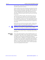
Symbols Used in This Manual
Symbol
Meaning
Indicates a PRO/II input coding note. The number beside the
symbol indicates the section in the PRO/II Keyword Input
Manual to refer to for more information on coding the
input file.
Indicates an important note.
Indicates a list of references.
Int-2
Introduction
May 1994
This page intentionally left blank.
II-2
May 1994
Section 2.1
2.1
Flash Calculations
Flash Calculations
PRO/II contains calculations for equilibrium flash operations such as flash
drums, mixers, splitters, and valves. Flash calculations are also used to determine
the thermodynamic state of each feed stream for any unit operation. For a flash calculation on any stream, there are a total of NC + 3 degrees of freedom, where NC is the
number of components in the stream. If the stream composition and rate are fixed,
then there are 2 degrees of freedom that may be fixed. These may, for example, be
the temperature and pressure (an isothermal flash). In addition, for all unit operations, PRO/II also performs a flash calculation on the product streams at the outlet
conditions. The difference in the enthalpy of the feed and product streams constitutes
the net duty of that unit operation.
PRO/II Unit Operations Reference Manual
II-3
Flash Calculations
2.1.1
Section 2.1
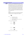
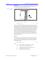
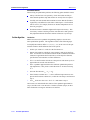
Basic Principles
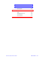
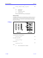
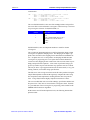
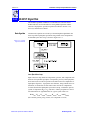
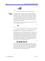
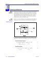
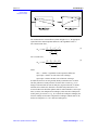
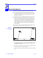
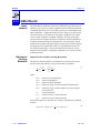
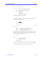
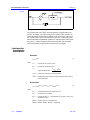
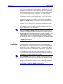
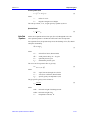
Figure 2.1.1-1 shows a three-phase equilibrium flash.
Figure 2.1.1-1:
Three-phase
Equilibrium Flash
MESH
Equations
The Mass balance, Equilibrium, Summation, and Heat balance (or MESH)
equations which may be written for a three-phase flash are given by:
Total Mass Balance:
F = V + L1 + L2
(1)
Component Mass Balance:
Fzi = Vyi + L1 + L2
(2)
Equilibrium:
yi = K1i x1i
(3)
yi = K2i x2i
(4)
x1i =
K2i
x
K1i 2i
(5)
Summations:
∑
i
∑
i
II-4
Basic Principles
yi − ∑ x1i = 0
(6)
i
yi − ∑ x2i = 0
(7)
i
May 1994
Section 2.1
Flash Calculations
Heat Balance:
FHf + Q = VHv + L1H1l + L2H2l
Two-phase
Isothermal Flash
Calculations
(8)
For a two-phase flash, the second liquid phase does not exist, i.e., L2 = 0,
and L1 = L in equations (1) through (8) above. Substituting in equation (2)
for L from equation (1), we obtain the following expression for the liquid
mole fraction, xi:
xi =
(9)
zi
V
(Ki − 1) + 1
F
The corresponding vapor mole fraction is then given by:
yi = Kixi
(10)
The mole fractions, xi and yi sum to 1.0, i.e.:
∑
i
xi = ∑ yi = 1.0
(11)
i
However, the solution of equation (11) often gives rise to convergence difficulties for problems where the solution is reached iteratively. Rachford and Rice in
1952 suggested that the following form of equation (11) be used instead:
∑
i
yi − ∑ xi = ∑
i
i
(Ki − 1) zi
(Ki − 1)
V
+1
F
(12)
≤ TOL
Equation (12) is easily solved iteratively by a Newton-Raphson technique,
with V/F as the iteration variable.
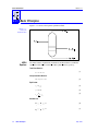
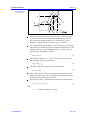
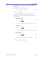
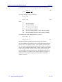
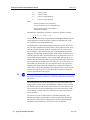
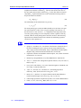
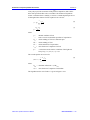
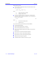
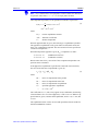
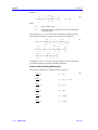
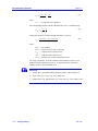
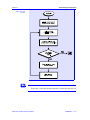
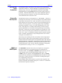
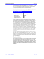
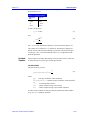
Figure 2.1.1-2 shows the solution algorithm for a two-phase isothermal flash,
i.e., where both the system temperature and pressure are given. The following steps outline the solution algorithm.
1.
The initial guesses for component K-values are obtained from ideal
K-value methods. An initial value of V/F is assumed.
2.
Equations (9) and (10) are then solved to obtain xi’s and yi’s.
3.
After equation (12) is solved within the specified tolerance, the composition convergence criteria are checked, i.e., the changes in the vapor and
liquid mole fraction for each component from iteration to iteration are
calculated:
| (yi,ITER − yi,ITER−1) |
yi
PRO/II Unit Operations Reference Manual
≤ TOL
(13)
Basic Principles
II-5
Flash Calculations
Section 2.1
Figure 2.1.1-2:
Flowchart for
Two-phase T, P
Flash Algorithm
II-6
Basic Principles
May 1994
Section 2.1
Flash Calculations
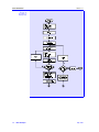
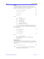
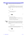
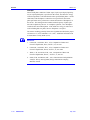
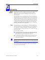
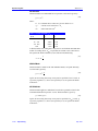
Figure 2.1.1-2:, continued
Flowchart for
Two-phase T, P
Flash Algorithm
| (xi,ITER − xi,ITER−1) |
xi
(14)
≤ TOL
4.
If the compositions are still changing from one iteration to the next, a
damping factor is applied to the compositions in order to produce a stable
convergence path.
5.
Finally, the VLE convergence criterion is checked, i.e., the following condition must be met:
| ∑ y − ∑ x
i
|
− ∑ yi − ∑ xi
≤ TOL
ITER
ITER−1
i
(15)
If the VLE convergence criterion is not met, the vapor and liquid mole
fractions are damped, and the component K-values are re-calculated. Rigorous K-values are calculated using equation of state methods, generalized
correlations, or liquid activity coefficient methods.
6.
A check is made to see if the current iteration step, ITER, is greater than the
maximum number of iteration steps ITERmax. If ITER > ITERmax, the flash
has failed to reach a solution, and the calculations stop. If ITER < ITERmax,
the calculations continue.
7.
Steps 2 through 6 are repeated until the composition convergence criteria and
the VLE criterion are met. The flash is then considered solved.
8.
Finally, the heat balance equation (8) is solved for the flash duty, Q, once
V and L are known.
PRO/II Unit Operations Reference Manual
Basic Principles
II-7
Flash Calculations
Flash
Tolerances
Section 2.1
The flash equations are solved within strict tolerances. All these tolerances
are built into the PRO/II flash algorithm, and may not be input by the user.
Table 2.1.1-1 shows the values of the tolerances used in the algorithm for the
Rachford-Rice equation (12), the composition convergence equations (13)
and (14), and the VLE convergence equation (15).
Table 2.1.1-1: Flash Tolerances
Equation
Bubble Point
Flash Calculations
Tolerance
Rachford-Rice (12)
1.0e-05
Composition Convergence
(13-14)
1.0e-03
VLE Convergence (15)
1.0e-05
For bubble point flashes, the liquid phase component mole fractions, xi, still
equal the component feed mole fraction, zi. Moreover, the amount of vapor,
V, is equal to zero. Therefore, the relationship to be solved is:
∑i Kizi = ∑i yi = 1.0
(16)
The bubble point temperature or pressure is to be found by trial-and-error
Newton-Raphson calculations, provided one of them is specified.
The K-values between the liquid and vapor phase are calculated by the thermodynamic method selected by the user. Equation (16) can, however, be
highly non-linear as a function of temperature as K-values typically vary as
exp(1/T). For bubble point temperature calculations, where the pressure and
feed compositions has been given, and only the temperature is to be determined, equation (16) can be rewritten as:
ln∑ Ki zi = 0
i
(17)
Equation (17) is more linear in behavior than equation (16) as a function of
temperature, and so a solution can be achieved more readily.
Equation (16) behaves in a more linear fashion as a function of pressure as
the K-values vary as 1/P. For bubble point pressure calculations, where the
temperature and feed compositions have been given, the equation to be
solved can be written as:
∑
Kizi − 1 = 0
(18)
i
II-8
Basic Principles
May 1994
Section 2.1
Dew Point Flash
Calculations
Flash Calculations
A similar technique is used to solve a dew point flash. The amount of vapor,
V, is equal to 1.0. Simplification of the mass balance equations result in the
following relationship:
∑i zi / Ki = ∑ xi = 1.0
(19)
i
For dew point pressure calculations, equation (19) can be linearized by writing it as :
ln ∑
i
zi
=0
Ki
(20)
For dew point temperature calculations, equation (19) may be rewritten as:
∑
i
zi
−1=0
Ki
(21)
The dew point temperature or pressure is then found by trial-and-error Newton-Raphson calculations using equations (20) or (21).
Two-phase
Adiabatic Flash
Calculations
For a two-phase, adiabatic (Q=0) system, the heat balance equation (8) can
be rewritten as:
1−
Hv
Hf
V Hl
− 1 − ≤ TOL
F
Hf
(22)
An iterative Newton-Raphson technique is used to solve the Rachford-Rice
equation (12) simultaneously with equation (22) using V/F and temperature
as the iteration variables.
Water Decant
The water decant option in PRO/II is a special case of a three-phase flash. If this
option is chosen, and water is present in the system, a pure water phase is decanted
as the second liquid phase, and this phase is not considered in the equilibrium flash
computations. This option is available for a number of thermodynamic calculation
methods such as Soave-Redlich-Kwong or Peng-Robinson.
Note: The free-water decant option may only be used with the Soave-RedlichKwong, Peng-Robinson, Grayson-Streed, Grayson-Streed-Erbar, Chao-Seader,
Chao-Seader-Erbar, Improved Grayson-Streed, Braun K10, or Benedict-WebbRubin-Starling methods. Note that water decant is automatically activated
when any one of these methods is selected.
PRO/II Unit Operations Reference Manual
Basic Principles
II-9
Flash Calculations
Section 2.1
The water-decant flash method as implemented in PRO/II follows these steps:
20.6
1.
Water vapor is assumed to form an ideal mixture with the hydrocarbon vapor phase.
2.
Once either the system temperature, or pressure is specified, the initial
value of the iteration variable, V/F is selected and the water partial pressure is calculated using one of two methods.
3.
The pressure of the system, P, is calculated on a water-free basis, by
subtracting the water partial pressure.
4.
A pure water liquid phase is formed when the partial pressure of water
reaches its saturation pressure at that temperature.
5.
A two phase flash calculation is done to determine the hydrocarbon vapor
and liquid phase conditions.
6.
The amount of water dissolved in the hydrocarbon-rich liquid phase is
computed using one of a number of water solubility correlations.
7.
Steps 2 through 6 are repeated until the iteration variable is solved within
the specified tolerance.
PRO/II Note: For more information on using the free-water decant option, see
Section 20.6, Free-Water Decant Considerations, of the PRO/II Keyword Input
Manual.
References
II-10
Basic Principles
1.
Perry R. H., and Green, D.W., 1984, Chemical Engineering Handbook, 6th Ed.,
McGraw-Hill, N.Y.
2.
Rachford, H.H., Jr., and Rice, J.D., 1952, J. Petrol. Technol., 4 sec.1, 19,
sec. 2,3.
3.
Prausnitz, J.M., Anderson, T.A., Grens, E.A., Eckert, C.A., Hsieh, R., and
O’Connell, J.P., 1980, Computer Calculations for Multicomponent VaporLiquid and Liquid-Liquid Equilibria, Prentice-Hall, Englewood Cliffs, N.J.
May 1994
Section 2.1
Three-phase
Flash
Calculations
Flash Calculations
For three-phase flash calculations, with a basis of 1 moles/unit time of feed,
F, the MESH equations are simplified to yield the following two nonlinear
equations:
| f1(L1, L2) | = | ∑ai zi / di | ≤ tolerance
(23)
i
| f1(L1, L2) | = | ∑bi zi / di | ≤ tolerance
(24)
i
where:
ai = (1 − K1i)
(25)
bi = (1 − K2i) (K1i / K2i)
(26)
di = K1i + ai L1 + bi L2
(27)
Equations (23) through (27) are solved iteratively using a Newton-Raphson
technique to obtain L1 and L2. The solution algorithm developed by SimSci
is able to rigorously predict two liquid phases. This algorithm works well
even near the plait point, i.e., the point on the ternary phase diagram where a
single phase forms.
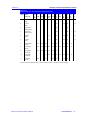
Table 2.1.1-1 shows the thermodynamic methods in PRO/II which are able to
handle VLLE calculations. For most methods, a single set of binary
interaction parameters is inadequate for handling both VLE and LLE equilibria. The PRO/II databanks contain separate sets of binary interaction parameters for VLE and LLE equilibria for many of the thermodynamic
methods available in PRO/II, including the NRTL and UNIQUAC liquid activity methods. For best results, the user should always ensure that separate
binary interaction parameters for VLE and LLE equilibria are provided for
the simulation.
Table 2.1.1-1:
VLLE Predefined Systems and K-value Generators
K-value Method
SRK1
SRKM
SRKKD
SRKH
SRKP
SRKS
PR1
PRM
PRH
PRP
UNIWAALS
IGS
GSE
CSE
HEXAMER
1
AMINE
NRTL
UNIQUAC
UNIFAC
UFT1
UFT2
UFT3
UNFV
VANLAAR
MARGULES
REGULAR
FLORY
SOUR
GPSWATER
LKP
System
SRK1
SRKM
SRKKD
SRKH
SRKP
SRKS
PR1
PRM
PRH
PRP
UNIWAALS
IGS
GSE
CSE
AMINE
HEXAMER
NRTL
UNIQUAC
UNIFAC
UFT1
UFT2
UFT3
UNFV
VANLAAR
MARGULES
REGULAR
FLORY
ALCOHOL
GLYCOL
SOUR
GPSWATER
LKP
VLLE available, but not recommended
PRO/II Unit Operations Reference Manual
Basic Principles
II-11
Flash Calculations
2.1.2
Section 2.1
Equilibrium Unit Operations
Flash
Drum
The flash drum unit can be operated under a number of different fixed conditions; isothermal (temperature and pressure specified), adiabatic (duty specified), dew point (saturated vapor), bubble point (saturated liquid), or isentropic
(constant entropy) conditions. The dew point may also be determined for the hydrocarbon phase or for the water phase. In addition, any general stream specification such as a component rate or a special stream property such as sulfur content
can be made at either a fixed temperature or pressure. For the flash drum unit,
there are two other degrees of freedom which may be set by imposing external
specifications. Table 2.1.2-1 shows the 2-specification combinations which may
be made for the flash unit operation.
Table 2.1.2-1:
Constraints in Flash Unit Operation
Flash Operation
Specification 1
ISOTHERMAL
TEMPERATURE
PRESSURE
DEW POINT
TEMPERATURE
PRESSURE
V=1.0
V=1.0
BUBBLE POINT
TEMPERATURE
PRESSURE
V=0.0
V=0.0
ADIABATIC
TEMPERATURE
PRESSURE
FIXED DUTY
FIXED DUTY
ISENTROPIC
TEMPERATURE
PRESSURE
FIXED ENTROPY
FIXED ENTROPY
TPSPEC
TEMPERATURE
GENERAL STREAM
SPECIFICATION
GENERAL STREAM
SPECIFICATION
PRESSURE
II-12
Specification 2
Equilibrium Unit Operations
May 1994
Section 2.1
Flash Calculations
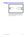
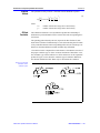
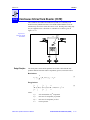
Valve
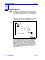
Figure 2.1.2-1:
Valve Unit
The valve unit operates in a similar manner to an adiabatic flash. The outlet
pressure, or the pressure drop across the valve is specified, and the temperature of the outlet streams is computed for a total duty specification of 0. The
outlet product stream may be split into separate phases. Both VLE and VLLE
calculations are allowed for the valve unit. One or more feed streams are allowed for this unit operation.
Mixer
Figure 2.1.2-2:
Mixer Unit
The mixer unit is, like the valve unit operation, solved in a similar manner to
that of an adiabatic flash unit. In this unit, the temperature of the single outlet stream is computed for a specified outlet pressure and a duty specification
of zero. The number of feed streams permitted is unlimited. The outlet product stream will not be split into separate phases.
PRO/II Unit Operations Reference Manual
Equilibrium Unit Operations
II-13
Flash Calculations
Section 2.1
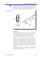
Splitter
Figure 2.1.2-3:
Splitter Unit
The temperature and phase of the one or more outlet streams of the splitter
unit are determined by performing an adiabatic flash calculation at the specified pressure, and with duty specification of zero. The composition and
phase distribution of each product stream will be identical. One feed stream
or a mixture of feed streams are allowed.
II-14
Equilibrium Unit Operations
May 1994
Section 2.2
2.2
Isentropic Calculations
Isentropic Calculations
PRO/II contains calculation methods for the following single stage constant
entropy unit operations:
Compressors (adiabatic or polytropic efficiency given)
Expanders (adiabatic efficiency specified)
PRO/II Unit Operations Reference Manual
II-17
Isentropic Calculations
2.2.1
Section 2.2
Compressor
General
Information
PRO/II contains calculations for single stage, constant entropy (isentropic) operations such as compressors and expanders. The entropy data needed for these calculations are obtained from a number of entropy calculation methods available in
PRO/II. These include the Soave-Redlich-Kwong cubic equation of state, and the
Curl-Pitzer correlation method. Table 2.2.1-1 shows the thermodynamic systems
which may be used to generate entropy data. User-added subroutines may also
be used to generate entropy data.
Table 2.2.1-1: Thermodynamic Generators for Entropy
Generator
Curl-Pitzer
Phase
1
VL
Lee-Kesler (LK)
VL
Lee-Kesler-Plöcker (LKP)
VL
LIBRARY
L
Soave Redlich-Kwong (SRK)
VL
Peng-Robinson (PR)
VL
SRK Kabadi-Danner (SRKKD)
VL
SRK and PR Huron-Vidal (SRKH, PRH)
VL
SRK and PR Panagiotopoulos-Reid (SRKP, PRP)
VL
SRK and PR Modified (SRKM, PRM)
VL
SRK SimSci (SRKS)
VL
UNIWAALS
VL
Benedict-Webb-Rubin-Starling (BWRS)
VL
Hexamer
VL
Hayden O’Connell (HOCV)
V
Truncated Virial (TVIRIAL)
V
Ideal-gas Dimer (IDIMER)
V
1
The Curl-Pitzer method is used to calculate entropies for a number of thermodynamic systems. For
example, by choosing the keyword SYSTEM=CS, Curl-Pitzer entropies are selected.
Once the entropy data are generated (see Section 1.2.1 of this manual, Basic
Principles), the condition of the outlet stream from the compressor and the
compressor power requirements are computed, using either a user-input adiabatic or polytropic efficiency.
II-18 Compressor
May 1994
Section 2.2
Basic Calculations
Isentropic Calculations
For a compression process, the system pressure P is related to the volume V by:
(1)
n
PV = Constant
where:
n=
exponent
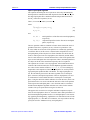
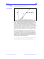
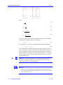
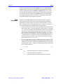
Figure 2.2.1-1 shows a series of these pressure versus volume curves as a
function of n.
Figure 2.2.1-1:
Polytropic
Compression Curve
The curve denoted by n=1 is an isothermal compression curve. For an ideal
gas undergoing adiabatic compression, n is the ratio of specific heat at constant pressure to that at constant volume, i.e.,
n = k = cp / cv
(2)
where:
k=
ideal gas isentropic coefficient
cp =
specific heat at constant pressure
cv =
specific heat at constant volume
For a real gas, n > k.
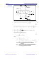
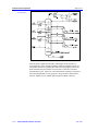
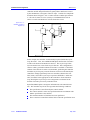
The Mollier chart (Figure 2.2.1-2) plots the pressure versus the enthalpy, as a
function of entropy and temperature. This chart is used to show the methods
used to calculate the outlet conditions for the compressor as follows:
PRO/II Unit Operations Reference Manual
Compressor II-19
Isentropic Calculations
Section 2.2
Figure 2.2.1-2:
Typical Mollier Chart
for Compression
A flash is performed on the inlet feed at pressure P1, and temperature
T1, using a suitable K-value and enthalpy method, and one of the entropy calculation methods in Table 2.2.1-1. The entropy S1, and enthalpy H1 are obtained and the point (P1,T1,S1,H1) is obtained.
The constant entropy line through S1 is followed until the user-specified
outlet pressure is reached. This point represents the temperature (T2) and
enthalpy conditions (H2) for an adiabatic efficiency of 100%. The adiabatic enthalpy change ∆Had is given by:
∆Had = H2 − H1
(3)
If the adiabatic efficiency, γad, is given as a value less than 100 %, the
actual enthalpy change is calculated from:
∆Hac = ∆Had / γad
(4)
The actual outlet stream enthalpy is then calculated using:
H3 = H1 + ∆Hac
(5)
Point 3 on the Mollier chart, representing the outlet conditions is then
obtained. The phase split of the outlet stream is obtained by performing
an equilibrium flash at the outlet conditions.
The isentropic work (Ws) performed by the compressor is computed from:
Ws = (H3 − H1) J = ∆Hac ∗ J
(6)
where:
J=
II-20 Compressor
mechanical equivalent of energy
May 1994
Section 2.2
Isentropic Calculations
In units of horsepower, the isentropic power required is:
GHPad = ∆Had ∗ 778 ∗ F / 33000
(7)
GHPac = ∆Hac ∗ 778 ∗ F / 33000 = GHPad / γad
(8)
HEADad = ∆Had ∗ 778
(9)
where:
GHP = work, hP
∆H =
enthalpy change, BTU/lb
F=
mass flow rate, lb/min
HEADad =
Adiabatic Head, ft
The factor 33000 is used to convert from units of ft-lb/min to units of hP.
The isentropic and polytropic coefficients, polytropic efficiency, and
polytropic work are calculated using one of two methods; the method from
the GPSA Engineering Data Book, and the method from the ASME Power
Test Code 10.
56
PRO/II Note: For more information on using the COMPRESSOR unit
operation, see Section 56, Compressor, of the PRO/II Keyword Input Manual.
ASME
Method
This method is more rigorous than the default GPSA method, and yields better
answers over a wider rage of compression ratios and feed compositions.
For a real gas, as previously noted, the isentropic volume exponent (also
known as the isentropic coefficient), ns, is not the same as the compressibility ratio, k. The ASME method distinguishes between k and ns for a real gas.
It rigorously calculates ns, and never back-calculates it from k.
Adiabatic Efficiency Given
In this method, the isentropic coefficient ns is calculated as:
ns = ln(P2 / P1) / ln(V1 / V2)
(10)
where:
V1 =
volume at the inlet conditions
V2 =
volume at the outlet pressure and inlet entropy conditions
The compressor work for a real gas is calculated from equation (8), and the
factor f from the following relationship:
(ns − 1 / ns)
Wac = 144 ns / ns − 1 f P1 V1 (P2 / P1)
− 1
(11)
The ASME factor f is usually close to 1. For a perfect gas, f is exactly equal
to 1, and the isentropic coefficient ns is equal to the compressibility factor k.
PRO/II Unit Operations Reference Manual
Compressor II-21
Isentropic Calculations
Section 2.2
The polytropic coefficient, n, is defined by:
n = ln(P2 / P1) / ln(V1 / V3)
(12)
where:
V3 =
volume at the outlet pressure and actual outlet enthalpy conditions
The polytropic work, i.e., the reversible work required to compress the gas in
a polytropic compression process from the inlet conditions to the discharge
conditions is computed using:
Wp = 144 (n / n−1) f P1 V1 (P2 / P1)
(n − 1 / n)
(13)
− 1)
where:
Wp =
polytropic work
For ideal or perfect gases, the factor f is equal to 1.
The polytropic efficiency is then calculated by:
γp = Ws / Wp
(14)
Note: This polytropic efficiency will not agree with the value calculated using the
GPSA method which is computed using γp = {(n-1)/n} / {(k-1)/k}.
Polytropic Efficiency Given
A trial and error method is used to compute the adiabatic efficiency, once the
polytropic efficiency is given. The following calculation path is used:
1.
The isentropic coefficient, isentropic work, and factor f are computed
using equations (10), (11), and (12).
2.
The polytropic coefficient is calculated from equation (12).
3.
An initial value of the isentropic efficiency is assumed.
4.
Using the values of f and n calculated from steps 1 and 2, the polytropic
work is calculated from equation (13).
5.
The polytropic efficiency is calculated using equation (14).
6.
If this calculated efficiency is not equal to the specified polytropic efficiency
within a certain tolerance, the isentropic efficiency value is updated.
7.
Steps 5 and 6 and repeated until the polytropic efficiency is equal to the
specified value.
Reference
American Society of Mechanical Engineers (ASME), 1965, Power
Test Code, 10, 31-33.
II-22 Compressor
May 1994
Section 2.2
Isentropic Calculations
GPSA
Method
This GPSA method is the default method, and is more commonly used in the
chemical process industry.
Adiabatic Efficiency Given
In this method, the adiabatic head is calculated from equations (3), (4), and
(9). Once this is calculated, the isentropic coefficient k is computed by trial
and error using:
(k−1 / k)
HEADac = (z1 + z2) / 2 RT1 / (k−1) / k (P2 / P1)
− 1
(15)
where:
z1, z2 = compressibility factors at the inlet and outlet conditions
R=
gas constant
T1 =
temperature at inlet conditions
This trial and error method of computing k produces inaccurate results when
the compression ratio, (equal to P2/P1) becomes low. PRO/II allows the user
to switch to another calculation method for k if the compression ratio falls
below a certain set value.
56
PRO/II Note: For more information on using the PSWITCH keyword to control
the usage of the isentropic calculation equation, see Section 56, Compressor,
of the PRO/II Keyword Input Manual.
If the calculated compression ratio is less than a value set by the user (defaulted
to 1.15 in PRO/II), or if k does not satisfy 1.0 ≤ k ≤ 1.66667, the isentropic coefficient, k, is calculated by trial and error based on the following:
T2 = (z1 / z2) T1 (P2 / P1)
(k−1) / k
(16)
The polytropic compressor equation is given by:
HEADp = (z1 + z2) / 2 RT1 / (n−1) / n (P2 / P1)
(n−1 / n)
− 1
(17)
The adiabatic head is related to the polytropic head by:
HEADad / γad = HEADp / γp
(18)
The polytropic efficiency n is calculated by:
γp = [n / (n−1)] / [k / (k−1)]
PRO/II Unit Operations Reference Manual
(19)
Compressor II-23
Isentropic Calculations
Section 2.2
The polytropic coefficient, n, the polytropic efficiency γp, and the polytropic
head are determined by trial and error using equations (17), (18), and (19)
above. The polytropic gas horsepower (which is reported as work in PRO/II)
is then given by:
GHPp = HEADp ∗ F / 33000
(20)
Polytropic Efficiency Given
A trial and error method is used to compute the adiabatic efficiency, once the
polytropic efficiency is given. The following calculation path is used:
1.
The adiabatic head is computed using equations (3), (4), and (9).
2.
The isentropic coefficient, k, is determined using equations (15), or (16).
3.
The polytropic coefficient, n, is then calculated from equation (19).
4.
The polytropic head is then computed using equation (17).
5.
The adiabatic efficiency is then obtained from equation (18).
Reference
GPSA, 1979, Engineering Data Book, Chapter 4, 5-9 - 5-10.
II-24 Compressor
May 1994
Section 2.2
2.2.2
Isentropic Calculations
Expander
General
Information
The methods used in PRO/II to model expander unit operations are similar to
those described previously for compressors. The calculations however, proceed in the reverse direction to the compressor calculations.
Basic
Calculations
The Mollier chart (Figure 2.2.2-1) plots the pressure versus the enthalpy, as a
function of entropy and temperature. This chart is used to show the methods
used to calculate the outlet conditions for the expander as follows:
Figure 2.2.2-1:
Typical Mollier Chart
for Expansion
A flash is performed on the inlet feed at the higher pressure P1, and temperature T1, using a suitable K-value and enthalpy method, and a suitable entropy calculation methods. The entropy S1, and enthalpy H1 are
obtained and the point (P1,T1,S1,H1) is obtained.
The constant entropy line through S1 is followed until the lower userspecified outlet pressure is reached. This point represents the temperature (T2) and enthalpy conditions (H2) for an adiabatic expander
efficiency of 100%. The adiabatic enthalpy change ∆Had is given by:
∆Had = H2 − H1
(1)
If the adiabatic efficiency, γad, is given as a value less than 100 %, the
actual enthalpy change is calculated from:
∆Hac = ∆Had / γad
PRO/II Unit Operations Reference Manual
(2)
Expander II-25
Isentropic Calculations
Section 2.2
The actual outlet stream enthalpy is then calculated using:
H3 = H1 + ∆Hac
(3)
Point 3 on the Mollier chart, representing the outlet conditions, is then
obtained. The phase split of the outlet stream is obtained by performing
an equilibrium flash at the outlet conditions.
The isentropic expander work (Ws) is computed from:
Ws = (H3 − H1) J = ∆Hac ∗ J
(4)
where:
J=
mechanical equivalent of energy
In units of horsepower, the isentropic expander power output is:
GHPac = ∆Had ∗ 778 ∗ F / 33000
(7)
GHPac = ∆Hac ∗ 778 ∗ F / 33000 = GHPad / γad
(8)
HEADad = ∆Had ∗ 778
(9)
where:
GHP = work, hP
∆H =
enthalpy change, BTU/lb
F=
mass flow rate, lb/min
HEADad =
Adiabatic Head, ft
The factor 33000 is used to convert from units of ft-lb/min to units of hP.
Adiabatic Efficiency Given
If an adiabatic efficiency other than 100 % is given, the adiabatic head is calculated from equations (3), (4), and (9). Once this is calculated, the isentropic coefficient k is computed by trial and error using:
(k−1 / k)
HEADac = (z1 + z2) / 2 RT1 / (k−1) / k (P2 / P1)
(10)
− 1
where
z1, z2 = compressibility factors at the inlet and outlet conditions
R=
gas constant
T1 =
temperature at inlet conditions
The polytropic expander equation is given by:
HEADp = (z1 + z2) / 2 RT1 / (n−1) / n (P2 / P1)
II-26 Expander
(n−1 / n)
− 1
(11)
May 1994
Section 2.2
Isentropic Calculations
The adiabatic head is related to the polytropic head by:
HEADad / γad = HEADp / γp
(12)
The polytropic efficiency n is calculated by:
γp = [n / (n−1)] / [k / (k−1)]
(13)
The polytropic coefficient, n, the polytropic efficiency γp, and the polytropic
head are determined by trial and error using equations (11), (12), and (13)
above. The polytropic gas horsepower output by the expander (which is reported as work in PRO/II) is then given by:
GHPp = HEADp ∗ F / 33000
PRO/II Unit Operations Reference Manual
(14)
Expander II-27
Isentropic Calculations
Section 2.2
This page intentionally left blank.
II-28 Expander
May 1994
Section 2.3
2.3
Pressure Calculations
Pressure Calculations
PRO/II contains pressure calculation methods for the following units:
Pipes (single and two-phase flows)
Pumps (incompressible fluids)
PRO/II Unit Operations Reference Manual
II-31
Pressure Calculations
Section 2.3
Pipes
2.3.1
General
Information
PRO/II contains calculations for single liquid or gas phase or mixed phase
pressure drops in pipes. The PIPE unit operation uses transport properties
such as vapor and/or liquid densities for single-phase flow, and surface
tension for vapor-liquid flow. The transport property data needed for these
calculations are obtained from a number of transport calculation methods
available in PRO/II. These include the PURE and PETRO methods for viscosities. Table 2.3.1-1 shows the thermodynamic methods which may be
used to generate viscosity and surface tension data.
Table 2.3.1-1: Thermodynamic Generators for
Viscosity and Surface Tension
Viscosity
Surface Tension
PURE (V & L)
PURE
PETRO (V & L)
PETRO
TRAPP (V & L)
API (L)
SIMSCI (L)
KVIS (L)
PRO/II contains numerous pressure drop correlation methods, and also
allows for the input of user-defined correlations by means of a user-added
subroutine.
Basic Calculations
An energy balance taken around a steady-state single-phase fluid flow
system results in a pressure drop equation of the form:
(dP / dL)t
total
=
(dP / dL)f
friction
+
(dP / dL)e
elevation
+
(dP / dL)acc
(1)
acceleration
The pressure drop consists of a sum of three terms:
the reversible conversion of pressure energy into a change in elevation
of the fluid,
the reversible conversion of pressure energy into a change in fluid
acceleration, and
the irreversible conversion of pressure energy into friction loss.
II-32 Pipes
May 1994
Section 2.3
Pressure Calculations
The individual pressure terms are given by:
(dP / dL)f = fρv / 2gcd
(2)
(dL / dL)e = gρsinφ / gc
(3)
(dP / dL)acc = ρv / gc dv / dL
(4)
2
where:
l and g refer to the liquid and gas phases
P=
the pressure in the pipe
L=
the total length of the pipe
d=
the diameter of the pipe
f=
friction factor
ρ=
fluid density
v=
fluid velocity
gc =
acceleration due to standard earth gravity
g=
acceleration due to gravity
φ=
angle of inclination
(dP/dL)t =
total pressure gradient
(dP/dL)f =
friction pressure gradient
(dP/dL)e =
elevation pressure gradient
(dP/dL)acc = acceleration pressure gradient
For two-phase flow, the density, velocity, and friction factor are often
different in each phase. If the gas and liquid phases move at the same
velocity, then the ‘‘no slip’’ condition applies. Generally, however, the
no-slip condition will not hold, and the mixture velocity, vm, is computed
from the sum of the phase superficial velocities:
vm = vsl + vgl
(5)
where:
vsl =
superficial liquid velocity = volumetric liquid
flowrate/cross sectional area of pipe
vgl =
superficial gas velocity = volumetric gas flowrate/cross
sectional area of pipe
Equations (2), (3), and (4) are therefore rewritten to account for these phase
property differences:
(dP / dL)f = ftp ρtp vtp / 2gc d
(6)
(dP / dL)e = gρtpsinφ / gc
(7)
(dP / dL)acc = ρtp vtp / gc (dvtp / dL)
(8)
2
PRO/II Unit Operations Reference Manual
Pipes II-33
Pressure Calculations
Section 2.3
where:
ρtp =
fluid density = ρlHL + ρgHg
H L , Hg =
Pressure Drop
Correlations
liquid and gas holdup terms subscript tp refers to the
two-phases
The hybrid pressure drop methods available in PRO/II each uses a separate
method to compute each contributing term in the total pressure drop equation
(1). These methods are described below.
Beggs-Brill-Moody (BBM)
This method is the default method used by PRO/II, and is the recommended
method for most systems, especially single-phase systems. For the pressure
drop elevation term, the friction factor, f, is computed from the relationship:
f / fn = ftp / fn = exp(s)
(9)
The exponent s is given by:
(10)
s = y / (−0.0523 + 3.182y − 0.8725y + 0.01853y )
2
y
4
(11)
y
s = ln(2.2e − 1.2), 1 < e < 1.2
(12)
2
y = ln(λL / HL)
where:
fn =
friction factor obtained from the Moody diagram for a
smooth pipe
λL =
no-slip liquid holdup = vsl/ (vsl + vsg)
vsl =
superficial liquid velocity
vsg =
superficial gas velocity
The liquid holdup term, HL, is computed using the following correlations:
b
c
HL0 = (aλL / NFr)
(13)
HL = HL0, when φ = 0
HL = HL0 Ψ, when φ ≠ 0
e f
g
3
Ψ = 1 + (1 − λL) lndλLNLv NFr sin(1.8φ) − 0.333sin (1.8φ)
(14)
where:
NFr =
Froude number
NLv =
liquid velocity number
a,b,c,d,e,f,g = constants
II-34 Pipes
May 1994
Section 2.3
Pressure Calculations
The BBM method calculates the elevation and acceleration pressure drop
terms using the relationships given in equations (3) and (4) (or equations (7)
and (8) for two-phase flow).
Beggs-Brill-Moody-Palmer (BBP)
This method uses the same elevation, and acceleration correlations described
above for the Beggs-Brill-Moody (BBM) method. The equation for the friction pressure drop term is the same as that given for the BBM method in
equations (9) through (12). For this method, however, the Palmer corection
factors given below are used to calculate the liquid holdup.
HL = 0.541 HL,BBM, φ < 0
HL = 0.918 HL,BBM, φ > 0
(15)
where:
HL,BBM =
liquid holdup calculated using the BBM method
Dukler-Eaton-Flanigan (DEF)
This method uses the Dukler correlation to calculate the friction term. The
friction factor is given by:
2
3
4
f / fn = 1 + y / 1.281 − 0.478y + 0.444y − 0.094y + 0.0084y
(16)
y = − ln(λL)
(17)
fn = 0.0056 + 0.5NRe
(18)
where:
NRe =
Reynolds number
The liquid holdup, HL, used in calculating the mixture density, ρ, in the friction term is computed using the Eaton correlation. In this correlation, the
holdup is defined as a function of several dimensionless numbers.
The elevation term is calculated using equation (3). The mixed density, ρ,
however, is calculated not by using the Eaton holdup, but by using the liquid
holdup calculated by the Flanigan correlation:
1.06
HL = 1 / 1 + 0.326 vsg
PRO/II Unit Operations Reference Manual
(19)
Pipes II-35
Pressure Calculations
Section 2.3
The acceleration term is calculated using the Eaton correlation:
2
2
(dP / dL)acc = W1∆v1 + Wg∆vg / 2gc qm ∆L
(20)
where:
W=
mass flow rate
v=
fluid velocity
vsg =
superficial gas velocity
qm =
mixture flow rate
subscripts g and l refer to the gas and liquid phases
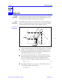
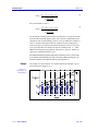
Mukherjee-Brill (MB)
The Mukherjee-Brill method is recommended for gas condensate systems. In
the MBN method, a separate friction pressure drop term is given for each region of flow. Figure 2.3.1-1 shows the various flow patterns which the MB
method is able to handle.
Figure 2.3.1-1:
Various Two-phase
Flow Regimes
For stratified flows in horizontal pipes:
(dp / dL)f = fρg vg / 2gc d
2
(21)
For bubble or slug flows:
2
(dP / dL)f = fρm vm / 2gc d
(22)
For mist flows:
2
(dP / dL)f = fffr ρg vg / 2gc d
(23)
where:
ffr =
II-36 Pipes
factor calculated from a correlation
May 1994
Section 2.3
Pressure Calculations
For bubble, slug, and mist flows, the elevation pressure drop is computed using equation (7), but for stratified flows, the fluid density used is the gas
phase density.
The acceleration pressure drop term is given by:
(dP / dL)acc = vm vs g ρtp / gc P(dP / dL)t
(24)
g
where:
vs =
slip velocity
The density, ρtp, is equal to the gas density for stratified flows only.
A separate expression is used to calculate the holdup for each flow pattern.
These are given as:
φ < 0 Bubble, Slug, Mist flow
N0.371771
H
GV
HL = e 2, H2 = H1 0.393962
NLV
(25)
2
(26)
2
H1 = −0.51664 + 0.789805 sinφ + 0.551627 sin φ + 15.519214 NL
φ < 0 Stratified flow
N0.079961
GV
HL = e , H2 = H1 0.604887
NLV
(27)
H2
2
2
H1 = −1.330282 + 4.808139 sinφ + 4.171584 sin φ + 56.262268 NL
(28)
φ ≥ 0 (all flow patterns)
N0.475686
GV
0.288657
NLV
(29)
HL = e 2, H2 = H1
H
2
2
H1 = −0.380113 + 0.129875 sinφ −0.119788 sin φ + 2.343227 NL
(30)
where:
NL =
PRO/II Unit Operations Reference Manual
liquid viscosity number
Pipes II-37
Pressure Calculations
Section 2.3
Gray
The Gray method has been especially developed for gas condensate wells,
and should not be used for horizontal piping. The recommended ranges for
use are:
Angle of inclination, φ = ≥ 70 degrees
Velocity, v < 50 ft/s,
Pipe diameter, d < 3.5 inches
Liquid condensate loading ~ 50 bbl/MMSCF
The friction pressure drop term is computed from equations (2) or (6), where
the friction factor used is obtained from the Moody charts. The elevation
term is calculated using equations (3) or (7), while the acceleration term is
given by equation (24).
The liquid holdup term, HL is given by:
HL = 1 − Hg
(31)
1
(32)
A
1−e
Hg =
R+1
B
1
205
A = −2.314 Nv 1 +
NC
1
0.730R
1
B = 0.0814 1 − 0.05554 ln1 +
R + 1
R=
(33)
(34)
(35)
VsL
Vsg
2
Nv =
(36)
2
ρm vsm
g σL (ρL − ρg)
2
g (ρl − ρg)D
ND =
σL =
(37)
σL
σ0 q0 + 0.617 σw qw
(38)
q0 + 0.617 qw
where:
σ=
surface tension
qo =
in situ oil volumetric flowrate
qw =
in situ water volumetric flowrate
qm =
mixture volumetric flowrate
ND =
diameter number
l (or L) and g (or G) refer to the liquid and gaseous phases
II-38 Pipes
May 1994
Section 2.3
Pressure Calculations
Oliemens
This method uses the Eaton correlation previously described above to
calculate the liquid holdup. The friction factor is obtained from the Moody
diagrams, and the friction pressure term is computed using:
(dP / dL)f = fG / 2 gc deff ρOLI 144
(39)
G = q1ρ1 + qgρg / (1 − BL) A
(40)
ρOLI = ρtp / (1 − BL)
(41)
BL = HL − HLns
(42)
2
where:
G=
mass flux
HLns = no-slip liquid holdup
ρOLI = Oliemens density
deff = effective diameter
A=
pipe cross sectional area
ρtp =
fluid density = ρlHL + ρgHg
l (or L) and g (or G) refer to the liquid and gas phases respectively
The acceleration term is set equal to zero, while the elevation pressure drop
term is computed using:
(dP / dL)e = ρs g sinφ / gc 144
(43)
ρs = ρ1HL + ρgHg, φ > 0
ρs = ρg, φ > 0 and HL < 1.0
ρs = ρ1, φ < 0 and HL = 1
(44)
where:
φ=
angle of inclination
subscripts l (or L) and g (or G) refer to the liquid and gas
phases respectively
Hagedorn-Brown (HB)
This method is recommended for vertical liquid pipelines, and should not be
used for horizontal pipes. The liquid holdup term is calculated from a correlation of the form:
HL = function of NlV, NGV, ND
(45)
where:
NlV, NGV, ND are the dimensionless liquid velocity number, gas
velocity number, and diameter number.
PRO/II Unit Operations Reference Manual
Pipes II-39
Pressure Calculations
Section 2.3
The friction factor is obtained from the Moody diagrams, and the friction
pressure term is computed using equations (2) or (6), depending on whether
there is single- or two-phase flow.
58
PRO/II Note: For more information on using these pressure drop correlation
methods in the PIPE unit operation, see Section 58, Pipe, of the PRO/II Keyword Input Manual.
References
1.
Beggs, H. D., An Experimental Study of Two-Phase Flow in Inclined Pipes,
1972, Ph.D. Dissertation, U. of Tulsa.
2.
Beggs, H. D., and Brill, J. P., A Study of Two-Phase Flow in Inclined Pipes,
1973, Trans. AIME, 607.
3.
Moody, L. F., Friction Factors for Pipe Flow, 1944, Trans. ASME,
66, 671.
4.
Palmer, C. M., Evaluation of Inclined Pipe Two-Phase Liquid Holdup
Correlations Using Experimental Data, 1975, M.S. Thesis, U. of Tulsa.
5.
Mukherjee, H. K., An Experimental Study of Inclined Two-Phase
Flow, 1979, Ph.D. Dissertation, U. of Tulsa.
6.
Gray, H. E., Vertical Flow Correlation in Gas Wells, 1974, in User Manual:
API 14B, Subsurface Controlled Safety Valve Sizing Computer Program.
7.
Flanigan, O., Effect of Uphill Flow on Pressure Drop in Design of
Two-Phase Gathering Systems, 1958, Oil & Gas J., March 10, 56.
8.
Eaton, B. A., The Prediction of flow Patterns, Liquid Holdup and Pressure
Losses Occurring During Continuous Two-Phase Flow in Horizontal
Pipes, 1966, Ph.D. Dissertation, U. of Texas.
9.
Dukler, A.E., et al., Gas-Liquid Flow in Pipelines, Part 1: Research Results,
Monograph NX-28, U. of Houston.
10. Hagedorn, A.R., and Brown, K.E., Experimental Study of Pressure
Gradients Occuring During Continuous Two-Phase Flow in Small
Diameter Vertical Conduits, 1965, J. Petr. Tech., Apr., 475-484.
II-40 Pipes
May 1994
Section 2.3
2.3.2
Pressure Calculations
Pumps
General
Information
The PUMP unit operation in PRO/II contains methods to calculate the
pressure and temperature changes resulting from pumping an incompressible
fluid.
52
PRO/II Note: For more information on using the PUMP unit operation, see
Section 52, Pump, of the PRO/II Keyword Input Manual.
Basic
Calculations
The GPSA pump equation is used to relate the horsepower required by the
pump to the fluid pressure increase:
HP = q ∆P / (1714.3 e)
(1)
where:
HP =
required pump power, hp
q=
volumetric flow rate, gal/min.
∆P =
pressure increase, psi
e=
percent efficiency
The factor 1714.3 converts the pump work to units of horsepower. The work
done on the fluid calculated from (1) above is added to the inlet enthalpy.
The temperature of the outlet fluid is then obtained by performing an adiabatic flash.
Note: The PUMP unit should only be used for incompressible fluids. Compressible fluids may be handled using the COMPRESSOR unit operation.
Reference
GPSA Engineering Data Book, 9th Ed., 5-9
PRO/II Unit Operations Reference Manual
Pumps II-41
Section 2.4
2.4
Distillation and Liquid-Liquid Extraction Columns
Distillation and Liquid-Liquid Extraction Columns
The PRO/II simulation program is able to model rigorous and shortcut distillation columns, trayed and packed distillation columns (random and structured
packings), as well as liquid-liquid extraction columns.
PRO/II Unit Operations Reference Manual
Distillation and Liquid-Liquid Extraction Columns II-45
Distillation and Liquid-Liquid Extraction Columns
2.4.1
Section 2.4
Rigorous Distillation Algorithms
General
Information
This chapter presents the equations and methodology used in the solution of
the distillation models found in PRO/II. It is recommended reading for those
who want a better understanding of how the distillation models are solved.
This chapter also explains how the intermediate printout relates to the equations being solved.
All of the distillation algorithms in PRO/II are rigorous equilibrium stage
models. Each model solves the heat and material balances and vapor-liquid
equilibrium equations. The features available include pumparounds, five condenser types, generalized specifications, and interactions with flowsheeting
unit operations such as the Controller and Optimizer. Reactive distillation is
available for distillation and liquid-extraction. Automatic water decant is
available for water/hydrocarbon systems.
Modelling a distillation column requires solving the heat and material balance equations and the phase equilibrium equations. PRO/II offers four different algorithms for modeling of distillation columns:
the Inside/Out (I/O) algorithm,
the Sure algorithm,
the Chemdist algorithm, and
the ELDIST algorithm.
For electrolyte systems the Eldist algorithm is available, and for liquid- liquid extractors the LLEX algorithm should be used. Eldist, Chemdist and the LLEX
also allow chemical reaction. Eldist is used when equilibrium electrolytic reactions are present. Chemdist and LLEX allow kinetic, equilibrium (non-electrolyte) and conversion reactions to occur on one or more stages.
For most systems, SimSci recommends using the I/O algorithm. When more
than one algorithm can be used to solve a problem, the I/O algorithm will
usually converge the fastest. The I/O algorithm can be used to solve most refinery problems, and is very fast for solving crude columns and main fractionators. The I/O algorithm also solves many chemical systems, and when
possible should be the first choice for systems with a single liquid phase.
The Sure algorithm in PRO/II is the same time proven algorithm as in PROCESS. This algorithm is particularly useful for hydrocarbon systems where water
is present. It is the best algorithm to solve ethylene quench towers which have
large water decants in the upper portion of the tower. The Sure algorithm is also
appropriate for many other refining and chemical systems.
II-46
Rigorous Distillation Algorithms
May 1994
Section 2.4
Distillation and Liquid-Liquid Extraction Columns
Chemdist is a new algorithm developed at SimSci for the simulation of
highly non-ideal chemical systems. Chemdist is a full Newton-Raphson
method, with complete analytic derivatives. This includes composition derivatives for activity and fugacity coefficients. Chemdist allows two liquid
phases to form on any stage in the column, and also supports a wide range of
two liquid phase condenser configurations. Chemdist with chemical reactions allows In-Line Procedures for non-power law kinetic reactions.
47
PRO/II Note: For more information on inputting reaction kinetics using In-Line
Procedures, see Section 47, Procedure Data, of the PRO/II Keyword Input
Manual.
Eldist is an extension of Chemdist for modeling distillation of aqueous electrolyte mixtures. The aqueous chemistry is solved using third party software
from OLI Systems. The electrolyte calculation computes true vapor-liquid equilibrium K-values, which are converted to apparent vapor-liquid equilibrium KValues. Eldist then uses these in the vapor-liquid equilibrium calculations.
General Column
Model
A schematic diagram of a complex distillation column is shown in Figure
2.4.1-1. A typical distillation column may have multiple feeds and side
draws, a reboiler, a condenser, pumparounds, and heater-coolers. The column configuration is completely defined; the number of trays and the locations of all feeds, draws, pumparounds and heater-coolers. Note that the
optimizer can change feed, draw and heater-cooler locations.
Figure 2.4.1-1:
Schematic of Complex
Distillation Column
PRO/II Unit Operations Reference Manual
Rigorous Distillation Algorithms II-47
Distillation and Liquid-Liquid Extraction Columns
Section 2.4
Trays are numbered from the top down. The condenser and reboiler are
treated as theoretical stages, and when present the condenser is stage one.
There are no ‘‘hard limits’’ on the number of feeds, draws, pumparounds etc.
This results from the PRO/II memory management system.
Table 2.4.1-1 shows the features available with each algorithm. Pumparounds
can be used for liquid and/or vapor. The return tray can be above or below the
draw tray. Note that when the pumparound return is mixed phase (liquid and vapor) that both the vapor and the liquid are returned to the same tray.
PRO/II provides hydrodynamic calculations for packings supplied by Norton
Co. and Sulzer Brothers. Both rating and design calculations are available.
In rating mode, the diameter and height of packing are specified and the pressure drop across the packed section is determined. In design mode, the
height of packing and the pressure drop are specified, and the packing diameter is calculated.
Tray rating and sizing is also available and may be performed for new and existing columns with valve, sieve and bubble cap trays. Valve tray calculations are done using the methods from Glitsch. Tray hydraulics for sieve
trays are calculated using the methods of Fair and for bubble cap trays with
the methods of Bolles. Rating and design calculations are available.
The I/O and Sure algorithms provide a free water decant option. This is used
in refinery applications to model water being decanted at the condenser or at
other stages in the distillation column.
Table 2.4.1-1: Features Overview for Each Algorithm
I/O
Sure
Chemdist
Pumparounds
Y
Y
N
N
N
Packed Column
Y
Y
Y
N
Y
Tray Rating/Sizing
Y
Y
Y
N
Y
Two Liquids on any tray
N
Y
Y
----
N
Free Water Decant
Y
Y
N
----
N
(2)
LLEX
Eldist
Tray Efficiency
Y
N
Y
N
Y(2)
Solids
Y
Y
Y
N
(1)
LS Components
N
N
N
N
Y
Electrolytes
N
N
N
N
Y
Kinetic Reaction
N
N
Y
Y
N
Equilibrium Reaction
N
N
Y
Y
N
Conversion Reaction
N
N
Y
Y
N
(1) Eldist predicts solids precipitation on stages, but does not allow solid formation for mass balance
purposes.
(2) Only vaporization efficiencies available.
II-48
Rigorous Distillation Algorithms
May 1994
Section 2.4
Distillation and Liquid-Liquid Extraction Columns
Side draws may be either liquid or vapor, and the location and phase of each
must be specified. Solid side draws are not allowed. There may be an unlimited number of products from each stage.
Feed tray locations are given as the tray number upon which the feed is introduced. A feed may be liquid, vapor or mixed phase. PRO/II also allows for
different conventions for mixed phase (vapor/liquid) feeds. The default convention NOTSEPARATE introduces both the liquid and the vapor to the
same stage. SEPARATE places the liquid portion of the feed on the designated feed tray and the vapor portion of the feed on the tray above the designated feed tray.
A pumparound is defined as a liquid or vapor stream from one tray to another. The return tray can be either above or below the pumparound draw
tray. The pumparound flowrate can be specified or calculated to satisfy a
process requirement. If a heater/cooler is used with the pumparound, it must
be located on the pumparound return tray. The pumparound return temperature, pressure, liquid fraction, and temperature drop will be computed if it is
not specified.
Heater/coolers may be located on any tray in the column. A heater/cooler is
treated only as a heat source or sink. Rigorous models of external heat exchangers are available via the attached heat exchanger option.
81
PRO/II Note: For more information on using attached heat exchangers, see Section 81, Simple Heat Exchanger, of the PRO/II Keyword Input Manual.
Feed rates, side draw rates and heater/cooler duties may be either fixed or
computed. For each varied rate or duty, a corresponding design specification
must be made.
Mathematical
Models
There are many different approaches to solving the distillation equations. This
is evident from the large number of articles on the subject in the chemical engineering literature. There are many classes of distillation problems; wide and narrow boiling, azeotropic, homogeneous and heterogeneous liquid phases,
electrolytic and reactive. Unfortunately, no one algorithm is yet available which
can reliably solve all of these problems. PRO/II provides different algorithms
which excel in solving certain classes of problems and often provide solution capability over a very wide range of problems. Eldist is designed to solve a specific class of problems, namely electrolytic systems. The LLEX (liquid-liquid
extractor) is for liquid liquid extraction systems.
PRO/II Unit Operations Reference Manual
Rigorous Distillation Algorithms II-49
Distillation and Liquid-Liquid Extraction Columns
Inside Out
Algorithm
Section 2.4
The Inside/Out (I/O) column algorithm in PRO/II is based on an article by
Russell in 1983. The I/O column algorithm contains a number of novel features which contribute to its excellent convergence characteristics. The algorithm is partitioned into an inner and outer loop. In the inner loop, the heat,
material and design specifications are solved. Simple thermodynamic models for enthalpy and vapor liquid equilibrium (VLE) K-values are used in the
inner loop. This, along with the form of the simple model and the choice of
primitive variables, allows the inner loop to be solved quickly and reliably.
In the outer loop, the simple thermodynamic model parameters are updated
based on the new compositions and the results of rigorous thermodynamic
calculations. When the rigorously computed enthalpies and K-values match
those of the simple thermodynamic models, and the design specifications are
met, the algorithm is solved.
Inner Loop
The primitive variables in the inner loop are the stripping factors and sidestream
withdrawal factors. The inner loop equations are the stage enthalpy balances
and the design specifications. The stripping factor here is defined as:
Kb V
Sj =
L j
(1)
where:
Sj =
the Stripping Factor for stage j
V=
the net vapor leaving the stage
L=
the net liquid leaving the stage
Kb =
the base component K-value from the simple K-value
model (see equation (11))
The inner loop solves the system of equations:
LSS
H1 = f S1, S2, ..., Sn,
=0
L k
LSS
H2 = f S1, S2, ..., Sn,
=0
L k
.
.
.
LSS
=0
Hn = f S1, S2, ..., Sn,
L
k
LSS
=0
SPk = f S1, S2, ..., Sn,
L
k
(2)
In equation (2) Hj is the heat balance for stage j:
II-50
Rigorous Distillation Algorithms
May 1994
Section 2.4
Distillation and Liquid-Liquid Extraction Columns
LSS
VSS
L
V
V
L
+ Hj Vj 1 +
Hj = Hj Lj 1 +
− Hj−1 Lj−1 − Hj+1 Vj+1
L
V
j
j
NF
(3)
NQ
− ∑ Hi Fi − ∑ Qi = 0
F
i=1
i=1
and SPk is a design specification equation.
This system of equations is solved using the Newton-Raphson method. The
first Jacobian matrix is obtained by finite difference approximation. This Jacobian is then inverted, and at subsequent iterations the inverse Jacobian is
updated using Broyden’s method.
To evaluate the errors in the enthalpy and specification equations for a given
set of stripping factors, the component flows and stage temperatures must be
computed for the given stripping factors and simple model parameters. Figure 2.4.1-2 shows a schematic diagram of a simple stage.
Figure 2.4.1-2:
Schematic of a Simple
Stage for I/O
Writing the material balance for this stage in terms of net liquid and vapor
flowrates results in:
LSS
VSS
−v
fj = −lj−1 + lj 1 +
+ v 1 +
Lj j Vj j+1
j
j
(4)
where:
PRO/II Unit Operations Reference Manual
l=
the component liquid rate, moles/time
v=
the component vapor rate, moles/time
f=
the component feed rate, moles/time
Rigorous Distillation Algorithms II-51
Distillation and Liquid-Liquid Extraction Columns
Section 2.4
Given the equilibrium relationship yi,j = Ki,j xi,j it is possible to remove v
from equation (4). This is done as follows:
vi,j = yi,jvj = Ki,j xi,j vj =
(5)
Ki,j vj li,j
Lj
where K is the vapor liquid equilibrium fugacity ratio. Now the component
mass balance can be written as:
Ki,j+1 Vj+1
LSS Ki,j Vj VSS
+
1
+
−l
fj = −li,j−1 + li,j 1+
L
i,
j
j+1
L Lj V
j
(6)
j
If K is assumed constant, equation (5) results in a linear system of equations
for component i which form a tridiagonal system:
Bi,1 Ci,1
Bi,2 Ci,2
−1
B
C
−1 i,3 i,3
⋅
⋅
⋅
−1 Bi,j−1 Ci,n−1
−1 Bi,n
li,1
li,2
l
i,3
⋅
⋅
⋅
li,n−1
l
i,n
(7)
fi,1
fi,2
f
i,3
⋅
⋅
⋅
fi,n−1
f
i,n
where B and C are given by:
LSS Ki,j Vj
VSS
Bi,j = 1 +
+ L 1 + V
L
j
j
j
(8)
Ki,j+1 Vj+1
Ci,j = −
Lj+1
(9)
Sidestream withdrawal factors are defined as:
LSS
RLj = 1 +
L j
VSS
RVj = 1+
V j
(10)
The vapor equilibrium K-value simple model is given by:
Ki,j = αij Kb
(11)
where αi,j is the relative volatility for component i on stage j and Kb is the
base component K-value modeled by:
1
1
ln(Kb) = A + B − ref
T T
II-52
Rigorous Distillation Algorithms
(12)
May 1994
Section 2.4
Distillation and Liquid-Liquid Extraction Columns
ref
In equation (12) T is a reference temperature. Using this definition of the
simple K-value model and the sidestream withdrawal factors, the material
balance (4) can be rewritten as:
fi,j = −li,j−1 + li,j (RL,j + ai,j SjRV,j) − li,j+1 (ai,j+1 Sj+1)
(13)
The set of equations defined by (13) still form a tridiagonal matrix so that
equation (7) still applies. Bij and Cij from (8) and (9) now become:
Bi,j = RL,j + αi,jSjRV j
Ci,j = −αi,j+1 Sj+1
(14)
Outer Loop
The outer loop in the Inside/Out algorithm updates the simple thermodynamic model parameters and checks for convergence. In the inner loop, the
distillation equations are solved for the current simple thermodynamic models. The convergence check in the outer loop therefore compares the rigorously computed enthalpies and VLE K-values from the new compositions
resulting from the inner loop calculations.
The simple model used for VLE K-values is given by equations (11) and
(12). The initial value of Kb on each stage j is computed by:
ln(Kb) = ∑ wi ln(Ki)
i
wi =
ti
∑ ti
i
ti = yi
δ(ln Ki)
1
δ
T
(15)
The simple K-values can be calculated very quickly for a given temperature.
Also, once new molar flows are computed in the inner loop, a new bubble
point temperature can be easily computed. Once the molar flows are computed, the mole fractions are obtained from:
xi,j =
(16)
li,j
∑ li,j
i
and substituting equation (11) into the bubble point equation:
∑ yi,j = ∑ Ki,j xi,j = 1
i
Kb =
(17)
i
1
(18)
∑ αixi
i
PRO/II Unit Operations Reference Manual
Rigorous Distillation Algorithms II-53
Distillation and Liquid-Liquid Extraction Columns
Section 2.4
Once Kb has been determined, equation (12) can be arranged so that the bubble
point temperature can be solved for directly. The bubble point expression is:
−1
bubble
T
(19)
ln(Kb − A)
1
=
+ ref
B
T
The simple enthalpy models are of the form:
0
Hv = Hv − ∆Hv
(20)
0
HL = HL − ∆HL
where:
Hv =
the vapor enthalpy
HL =
the liquid enthalpy
H0v =
the vapor ideal gas enthalpy
H0L =
the liquid ideal gas enthalpy
∆Hv = the vapor enthalpy departure from the ideal gas enthalpy
∆HL = the liquid enthalpy departure from the ideal gas enthalpy
The simple model for the enthalpy departure is given by:
ref
∆Hv = A + B(T − T )
∆HL = C + D(T − T )
ref
(21)
where the departures are modeled in terms of energy per unit mass.
The I/O algorithm has four different levels of intermediate iteration printout.
These are None, Part, Estimate, and All. None results in no iteration printout. Part results in partial intermediate printout, and is useful to monitor the
progress of the algorithm toward solution. Estimate should be used to debug
a non-converged column. Estimate prints the initial column estimate and
more information on actual equation errors to help determine what the convergence difficulty is. All prints out the column temperature, liquid and vapor profiles at each iteration and the same comprehensive intermediate
printout as Estimate.
II-54
Rigorous Distillation Algorithms
May 1994
Section 2.4
Distillation and Liquid-Liquid Extraction Columns
With Partial intermediate printout, the following information is provided at
each iteration:
ITER
ITER
1 E(K) =
INNER
INNER
2 E(K) =
INNER
INNER
1.0717E-01 E(ENTH+SPEC)=1.392E-03 E(SUM) = 3.159E-01
0 : E(ENTH+SPEC) = 1.104E-02
1 : E(ENTH+SPEC) = 1.854E-04 ALPHA = 1.0000
1.137E-02 E(ENTH+SPEC) = 1.854E-04 E(SUM) = 2.454E-02
0 : E(ENTH+SPEC) = 5.925E-04
1 : E(ENTH+SPEC) = 7.476E-06 ALPHA = 1.0000
The error E(ENTH+SPEC) is the sum of the enthalpy balance and specification errors and is used to determine convergence of the inner loop. The inner
loop convergence tolerance for E(ENTH+SPEC) is:
Iteration
E(ENTH+SPEC) Tolerance
1
0.01
2
0.001, (if E(ENTH+SPEC) error from iter 1
was below 0.001, then the tolerance =
2.0E-5)
3
2.0E-5
E(ENTH+SPEC) is the most important number to watch for column
convergence.
The second most important number to watch for information about column
convergence is alpha, the damping factor. The damping factor alpha is applied to the correction to the stripping factors and sidestream withdrawl factors. An alpha value of 1.0 corresponds to no damping and indicates that
convergence is progressing well. Low alpha values indicate that the full
correction to the stripping factors resulted in an increase in the inner loop enthalpy and specification equations. A line search is performed using a progressively smaller step size until the inner loop equation errors are reduced.
This may be due to a poor approximation to the Jacobian matrix, a very poor
starting estimate, or infeasible design specifications.
The E(K) error is the average error between the K-values predicted using the
simple thermodynamic model and the rigorously computed K-values using
the compostions and termperatures resulting from the inner loop calculations. A large E(K) indicates highly compostion sensititve K-values.
The error sum E(SUM) is the sum of the enthalpy, specification and the bubble point errors. This value is not used in the convergence check. E(SUM)
is a good indicator of how convergence is progressing, and is similiar to the
ERROR SUM for the Sure Algorithm.
With Estimate and All iteration printout levels, the following intermediate
printout results:
PRO/II Unit Operations Reference Manual
Rigorous Distillation Algorithms II-55
Distillation and Liquid-Liquid Extraction Columns
Section 2.4
ITER 1 E(K) = 1.017E-01 E(ENTH+SPEC)= 1.392E-03 E(SUM
) = 3.159E-01
COMPONENT ERROR: AVG = 4.491E-02 MAX(T 1
) = 1.814E-01
ENTHALPY ERROR: AVG = 0.000E+00 MAX(T 4, LIQ ) = 0.000E+00
K-VALUE ERROR: AVG = 1.017E-01 MAX(T 1, C 1
) = 3.31OE-01
INNER 0 : E(ENTH+SPEC) = 1.104E-02
SPEC ERROR : AVG = 1.134E-02 MAX(SPEC 1
) = 2.267E-02
HBAL ERROR : AVG = 5.368E-03 MAX(TRAY 2
) = -1.230E-02
TEMP CHANGE: AVG = 8.500E-01 MAX(TRAY 1
) = -2.461e+00
INNER 1: E(ENTH+SPEC) = 1.854E-04
ALPHA - 1.0000
SPEC ERROR : AVG = 1.886E-04 MAX(SPEC 1
) = 3.756E-04
HBAL ERROR : AVG = 9.114E-05 MAX(TRAY 3
) = 2.182E-04
TEMP CHANGE: AVG = 1.257E-01 MAX(TRAY 1
) = -2.431E-01
ITER 2 E(K) = 1.137E-02 E(ENTH+SPEC) = 1.854E-04 E(SUM ) = 2.454E-02
COMPONENT ERROR: AVG = 5.068E-03 MAX(T 1
) = 1.026e-02
ENTHALPY ERROR: AVG = 0.000E+00 MAX(T 4, LIQ
) = 0.999E+00
K-VALUE ERROR: AVG = 1.137E-02 MAX(T 1, C 2
) = 2.268E-02
INNER 0 : E(ENTH+SPEC) = 5.9253E-04
SPEC ERROR : AVG = 6.25E-04 MAX(SPEC 1
) = -1.247E-03
HBAL ERROR : AVG = 2.799E-04 MAX(TRAY 2
) = 5.961E-04
TEMP CHANGE: AVG = 3.719E-02 MAX(TRAY 1
) = -8.621E-02
INNER 1 : E(ENTH+SPEC) = 7.476E-06 ALPHA = 1.0000
SPEC ERROR : AVG = 8.569E-06 MAX(SPEC 1
) = -1.587E-05
HBAL ERROR : AVG = 3.191E-06 MAX(TRAY 2
) = 9.271E-06
TEMP CHANGE: AVG = 7.271E-03 MAX(TRAY 1
) = 1.253E-02
Reference
Russell, R.A., A Flexible and Reliable Method Solves Single-tower and
Crude-distillation -column Problems, 1983, Chem. Eng., 90, Oct. 17, 53-9.
Chemdist
Algorithm
The Chemdist algorithm in PRO/II is a Newton based method which is suited to
solving non-ideal distillation problems involving a smaller number (10 vs. 100) of
chemical species. These conditions are generally encountered in chemical distillations as opposed to crude fractionation where the I/O algorithm would be a better
choice. Chemdist is designed to handle both vapor-liquid and vapor-liquid-liquid
equilibrium problems as well as chemical reactions.
Figure 2.4.1-3:
Schematic of a
Simple Stage for Chemdist
II-56
Rigorous Distillation Algorithms
May 1994
Section 2.4
Distillation and Liquid-Liquid Extraction Columns
Basic Algorithm
Figure 2.4.1-3 shows a schematic of an equilibrium stage for the case of two
phase distillation with no chemical reaction. The equations which describe
the interior trays of the column are as follows:
Component Mass Balance:
D
Mi,j = exp (Xi,j)Li + exp(Yi,j)Vi − exp(Xi−1,j) Li−1 − Li−1
(22)
L
V
D
−exp (Yi+1,j) Vi+1 − Vi+1 − fi,j − fi−1,j i=1, NT, j=1, NC
Energy Balance:
^L
^V
^L
^V
D
D
Ei = LiHi + ViHi − Li−1 − Li−1 Hi−1 − Vi+1 − Vi+1 Hi+1
V ^ FV
L ^ FL
−Qi − Fi Hi − Fi+1 Hi+1, i=1, NT
(23)
Vapor-Liquid Equilibrium:
Qi,j = Yi,j − Xi,j − ln(Ki,j)
i = 1,NT and j = 1,NC
(24)
Summation of Mole Fractions:
NL
Si = 1 − ∑ exp (Xi,j)
(25)
i = 1,NT
j=1
(26)
NC
Si′ = 1 − ∑ exp(Yi,j)
i = 1,NT
j=1
where:
Fi =
total feed flow to tray i
Li =
total liquid flow from tray i
Vi =
total vapor flow from tray i
Qi =
heat added to tray i
Ti =
temperatures of tray i
Xi,j =
ln(xi,j) natural log of the liquid mole fractions
Yi,j =
ln(yi,j) natural log of the vapor mole fractions
NC =
number of components
NT =
number of trays
subscripts:
PRO/II Unit Operations Reference Manual
i=
tray index
j=
component index
Rigorous Distillation Algorithms II-57
Distillation and Liquid-Liquid Extraction Columns
Section 2.4
superscripts:
F=
refers to a feed
D=
refers to a draw
L=
refers to a liquid property
V=
refers to a vapor property
other:
^ refers to properties on a molar basis
lower case letters refer to component flows
upper case letters refer to total flows or
transformed variables
The unknowns, alternatively referred to as iteration or primitive variables:
( X , Y , L , V , T )i , where i = 1,NT
are solved for directly using an augmented Newton-Raphson method. Specification equations involving the iteration variables are added directly to the
above equations and solved simultaneously.
The modifications of the Newton-Raphson method are twofold. The first is a
line search procedure that will, when possible, decrease the sum of the errors
along the Newton correction. If this is not possible, the size of the increase
will be limited to a prescribed amount. The second modification limits the
changes in the individual iteration variables. Both of these modifications can
result in a fractional step in the Newton direction. The fractional step size, is
reported in the iteration summary of the column output. Note that an α of 1
indicates that the solution procedure is progressing well and that, as the solution is approached, α should become one. In the case of very non-linear systems which may oscillate, the user can restrict the step size by specifying a
damping factor which reduces the changes in the composition variables. A
cutoff value is used by the algorithm so that when the value of the sum of the
errors drops below the given level, the full Newton correction is used. This
serves to speed the final convergence.
74
PRO/II Note: For more information on using the damping factor and setting the
size of the error increase, see Section 74, Chemdist, of the PRO/II Keyword Input Manual.
The iteration history also reports the largest errors in the mass balance, the
energy balance, and the vapor-liquid equilibrium equations. Given a good initial estimate, these should decrease from iteration to iteration. However, for
some systems, the errors will temporarily increase before decreasing on the
way to finding a solution. The user can limit the size of the increase in the
sum of the errors.
All derivatives for the Jacobian matrix are calculated analytically. Useradded thermodynamic options that are used by Chemdist must provide partial derivatives with respect to component mole fractions and temperature.
Chemdist uses the chain rule to convert these to the needed form.
II-58
Rigorous Distillation Algorithms
May 1994
Section 2.4
Distillation and Liquid-Liquid Extraction Columns
Vapor-Liquid-Liquid Algorithm
The equations describing the VLLE system are derived by substituting the
bulk liquid flows and transformed bulk liquid mole fractions, Li and Xi,j, for
the single liquid phase flows and the transformed liquid mole fractions, Li
and Xi,j, in the above equations (22-26).
That is, Li becomes Li and Xi,j becomes Xi,j.
where:
__
Xi,j = ln (l′i,j + l′′i,j) ⁄ (L′i,j + L′′i,j)
_
Li = L′i + L′′i
(27)
(28)
and:
L′i , L"i =
total liquid flows of the first and second liquid phases,
respectively.
l′i,j , l"i,j =
component liquid flows in the first and second liquid
phases, respectively.
The new equations which are identical in form to those listed in the basic algorithm section above, equations (22-26), will not be repeated here. The
K-values which are used in the VLE equations are calculated by performing
a LLE flash. That is, the K-value is evaluated at the composition of one of
the liquid phases produced by the LLE flash. Chemdist uses the K-value derivatives with respect to the two liquid phases, the chain rule, and the definition of a total derivative to calculate the derivatives of the VLE equation with
respect to the bulk liquid flow and composition. That is, the bulk liquid flows
are subject to the all of the constraints imposed by the LLE equations.
The equations are solved in a two-step approach. After initialization and calculation of the Jacobian matrix, the Newton-Raphson algorithm calculates
new values for the iteration variables ( X , Y , L , V , T )i. The resulting tray
temperatures and composition of the bulk liquid phases are used in performing liquid-liquid equilibrium flash calculations. If a single liquid phase exists, the calculations proceed as in the basic algorithm. If a second liquid
phase is detected, the liquid compositions of the two liquid phases are used
to calculate the K-values and the derivatives with respect to each liquid
phase. Using the chain rule and the definition of a total derivative, these composition derivatives are used to calculate the derivative of the VLE equations
with respect to the bulk liquid phase. A new Jacobian matrix is calculated
and the Newton-Raphson algorithm calculates new values for the iteration
variables. The cycle repeats until convergence is achieved.
This approach is not as direct as using the individual component compositions for each liquid phase. However, it results in more stable performance of
the Newton-Raphson algorithm because a second liquid phase is not continually appearing and disappearing. Liquid draws are dealt with in terms of bulk
liquid properties (i.e., other than for a condenser, it is not possible to directly
specify the selective withdrawal of any one liquid phase).
PRO/II Unit Operations Reference Manual
Rigorous Distillation Algorithms II-59
Distillation and Liquid-Liquid Extraction Columns
Section 2.4
References:
Reactive
Distillation
Algorithm
1.
Bondy, R.W., 1991, Physical Continuation Approaches to Solving Reactive
Distillation Problems, paper presented at 1991 AIChE Annual meeting.
2.
Bondy, R.W., 1990, A New Distillation Algorithm for Non-Ideal System,
paper presented at AIChE 1990 Annual Meeting.
3.
Shah, V.B., and Bondy, R.W., 1991, A New Approach to Solving Electrolyte
Distillation Problems, paper presented at 1991 AIChE Annual meeting.
The Chemdist and LLEX algorithms in PRO/II support both liquid and vapor
phase chemical reactions. Since reactiive distillation is an extension of the
basic chemicals distillation algorithm, the reader should be familar with this
material before proceeding. In general, the extensions of the Chemdist and
LLEX algorithms for reactive distillation are suited to the same size systems,
i.e., distillation systems which have a smaller number (10 vs. 100) of chemical species. Larger systems can be simulated, but a large number of calculations can be expected.
Basic Algorithm
Figure 2.4.1-4 shows a schematic of an equilibrium stage for the case of twophase distillation with chemical reaction. The equations which describe the interior trays of the column on which reactions occur are essentially the basic
equations which have terms added for generation and consumption of chemical
species. The equilibrium equations will be affected only indirectly through the
formation or disappearance of chemical species. Similarly, the energy balance
equation is affected through the enthalpies of the species enthalpies. If two
chemicals react to form a third and produce heat in doing so, then the enthalpy
of the reaction product must be low enough to account for the disappearance of
the moles of the reacting species and the heat of reaction.
II-60
Rigorous Distillation Algorithms
May 1994
Section 2.4
Distillation and Liquid-Liquid Extraction Columns
Figure 2.4.1-4:
Reactive Distillation
Equilibrium Stage
The mass balance equations are the only equations which must have consumption and production terms added. The new equation is:
(29)
NF
Mi,j = exp(Xi,j)Lj + exp(Yi,j)Vj − exp(Xi,j−1)Lj−1 = exp(Yi,j + 1)Vj+1 − ∑ FkZi,k
k=1
NRxKj
NRxEq
NRxCnv
k=1
k=1
k=1
− ∑ Vi,krk −∑ Vi,k ε − ∑
Vi,k
εexp(XRef,j−1)Lj−1 + exp(YRef,j+1)Vj+1
VRef,k
The kinetic rates of reaction are given by:
(−
rk = k0 exp
A
)
RT
(30)
V∏ [A] [B] K
a
b
where:
V=
the reaction volume
A, B = denote chemical species A and B
a,b =
the stoichiometric coefficients of chemical species A and B
in the stoichiometric equation, respectively
exp(-A/RT) = the Arrhenius rate expression for temperature
dependence
Π=
PRO/II Unit Operations Reference Manual
denotes the product of the concentrations of the chemicals
raised to their stoichiometric coefficients.
Rigorous Distillation Algorithms II-61
Distillation and Liquid-Liquid Extraction Columns
Section 2.4
The only place the reaction volume is used in the distillation calculations is
in the kinetic rate expression (equation (30)). It is extremely important that
the tray reaction volumes are consistent with the volume basis used in determining the kinetic rate expression. If the reaction is a homogeneous liquid
phase reaction, and the rate expression is based on liquid phase reactions
done in a CSTR, then the liquid volume should be used. This volume corresponds to the liquid volume on the tray and in the downcomer. Do not use
the entire mechanical volume between trays unless the rate expression was
determined from pilot plant data and the entire volume was used to characterize the rate equation. Similarly, if the reaction is catalyzed by a metal on a
ceramic support and the rate equation was based on the entire cylindrical volume of the packed bed holding the catalyst, then this should be used.
Since the enthalpy basis in PRO/II is on a pure chemical basis, it is unsuitable for keeping track of enthalpy changes due to reactions. Therefore, reactive distillation converts chemical enthalpies to an elemental basis before
simulating the tower. After the simulation is complete, the product stream enthalpies are recalculated using the standard PRO/II basis. While this is
mostly hidden from the user, it does impact the reporting overall column enthalpy balance and is the reason for reporting multiple enthalpy balances.
This does not impact the accuracy of the solution.
Chemdist and LLEX support any type of reaction which can be entered
through the Reaction Data section or described using an in-line procedure.
Various reaction parameters may be varied from the flowsheet using calculators and DEFINE statements. Any set of mixed reactions may be assigned to
trays in the distillation column.
Chemdist and LLEX support single tray distillation columns. By using this
feature, Chemdist may be used as a two-phase reactor model which produces
vapor and liquid streams in equilibrium. In addition, the bottoms product rate
may be set to zero so that a boiling pot reactor can be modeled. As part of
this functionality, a single non-volatile component may be specified. The
non-volatile component is typically a catalyst which may used in the kinetic
reaction rate expressions.
Kinetic Reaction Homotopy (Volume Based)
The solution of the Mass, Equilibrium, Summation, and Enthalpy balance
equations can be a difficult task for non-ideal chemical systems. The addition
of reaction terms further complicates the challenge. Chemdist and LLEX
both have a homotopy procedure to simplify obtaining a solution to reactive
distillation columns. The basic procedure is straightforward:
Start with a set of equations to which you know the answer.
Then modifiy the equations a little and solve them.
Modify them again and re-solve using the last solution.
Eventually, the equations will be deformed into the equations to which you
want the answer.
II-62
Rigorous Distillation Algorithms
May 1994
Section 2.4
Distillation and Liquid-Liquid Extraction Columns
This procedure has a formalized mathematical basis with the theoretical underpinings beginning as early as 1869 (Ficken, 1951). Mathematically, a homotopy is a deformation or bending of one set of equations that are difficult
to solve, f{x} = 0, into a set whose solution is known or easily found,
g{x}=0. A new set of equations, referred to as the homotopy equations, is
constructed from f{x} and g{x}. The homotopy equations are what enable us
to move smoothly from the easy problem to the difficult problem. The most
general conditions for the homotopy equation are:
Hx,t = some function of f x and gx = 0
(31)
such that:
0
0
Hx ,0 = gx = 0
Hx∗,1 = fx∗ = 0
The simplest transformation is a linear homotopy. In this case, the homotopy
equation becomes:
Hx,t = tfx + (1−t) gx = 0
(32)
In equation (32), t is varied from zero to 1. The first challenge is choosing
the proper homotopy, the second is determining the sequence of t that allows
you to move from the simple equations to the difficult equations.
The methods for tracking the homotopy path from 0 to 1 are classified as either
‘‘simplicial’’, discrete methods, or ‘‘continuation’’, differential methods based
on the integration of an initial value method. Currently, the reactive distillation
algorithm in PRO/II uses a ‘‘classical’’ homotopy with a set of predefined steps.
In most cases involving reaction, this approach is sufficient.
The reactive distillation algorithm uses a physical homotopy with the reaction volume being linked directly to the homotopy parameter. That is, initially, the reaction volume is zero and the ‘‘simple’’ set of equations
corresponds to the basic distillation problem. At the final point, the reactive
volume is equal to the specified volume and the equations are the full set describing reactive distillation. This homotopy is only used for those systems
using a reaction volume. These are the most difficult systems to solve.
The actual function used to increase the reaction volume is a combination of
functions. Initially, there may not be any products present in the tower and
the reaction may proceed very quickly. Therefore, the volume is initially increased on a log fraction basis which very gradually introduces the reaction.
After the products begin to accumulate on the trays, the reaction volume is increased linearly. The transition between the two modes is at 25%.
PRO/II Unit Operations Reference Manual
Rigorous Distillation Algorithms II-63
Distillation and Liquid-Liquid Extraction Columns
Section 2.4
Summarizing, if the reaction homotopy is used, the initial problem is solved
with no chemical reaction on the trays. After the solution is reached, the reaction volume is increased by a small amount and the problem is resolved using the no reaction solution as a starting point. After the solution is reached,
the reaction volume is again increased and the problem is resolved. This continues until the reaction volume has been fully introduced. The number of increments and the initial volume may be specified by the user.
If the steps are small or the problem is not particularly difficult, the problems
at each volume are solved in a small number of iterations. Even with this, the
distillation equations are being solved at each volume step and it may take
quite a few iterations to solve. Other authors report increases in solution
times from 30% to 300% depending on the difficulty of the problem. In fairness, if the problem takes 3 times as long using the homotopy, the engineer
devoted a great deal of time generating the initial estimates in order to get
any solution. In many cases, there is no choice.
References
II-64
1.
Bondy, R.W., Physical Continuation Approaches to Solving Reactive
Distillation Problems, paper presented at 1991 AIChE Annual meeting.
2.
Ficken, F.A., 1951, The Continuation Method for Functional Equations,
Communications on Pure and Applied Mathematics, 4.
Rigorous Distillation Algorithms
May 1994
Section 2.4
Distillation and Liquid-Liquid Extraction Columns
Initial
Estimates
As previously mentioned, initial column profiles are needed for solution of
the column heat, mass, equilibrium, and performance specification balances.
These may either be provided by the user, or generated internally by PRO/II
using an initial estimate generator.
User-provided Estimates
Ideally, the only estimates the user has to provide is either the overhead rate
or the bottoms rate with the product information. On the other extreme, the
user can provide the complete estimates for the temperature, flowrates, and
composition profiles. PRO/II’s initial estimate generation (IEG) algorithms
generate these numbers relatively well and the user need not provide any initial estimates except for difficult simulations.
PRO/II could interpolate the temperature, liquid and vapor rates, and phase
compositions estimates, if the end point values for these variables are available. These end point values could either be provided by the user or estimated by PRO/II. When these values are provided by the user, we require
that the user provide at least two endpoint values (first and last theoretical
stage). The first theoretical stage is the condenser or the top tray for the ‘‘no
condenser’’ case. The last theoretical stage is the reboiler or the bottom tray
for the ‘‘no reboiler’’ case.
Temperatures
Tray temperatures are relatively easy to estimate. The reboiler and condenser temperatures represent the bubble points and/or dew points for the
products. These may be estimated by the user or calculated using the shortcut fractionator model.
The top and bottom tray temperatures may be estimated by addition or subtraction of a reasonable temperature difference from the condenser and reboiler temperatures.
For complex fractionators, the product draw temperatures are usually known
or can be estimated from the product ASTM distillations.
Liquid and Vapor Profiles
For most columns, the vapor and/or liquid profiles are more difficult to estimate. Moreover, they are generally more influential than temperatures in aiding or hindering the solution.
Estimates for the overhead or the bottoms products are provided with the
product information; in addition, rates for the side draw products are also provided by the user.
PRO/II Unit Operations Reference Manual
Rigorous Distillation Algorithms II-65
Distillation and Liquid-Liquid Extraction Columns
Section 2.4
For columns with condensers, it is important to provide an estimate of the reflux, either as the liquid from tray one or the vapor leaving tray two (the top
product plus reflux). For simple columns with liquid or moderately vaporized feeds, constant molar overflow may be assumed and the vapor from the
reboiler tray 6 assumed to be the same as the tray 2 vapor. The reboiler vapor may also be provided by giving an estimate of the liquid leaving the tray
above the reboiler.
For columns in which the feed has high vapor rate, there will be a sharp
break in the vapor profile at the feed tray. For such columns at least four vapor rates should be provided: top tray, feed tray, tray below feed, and bottom
tray.
For columns in which the reflux is to be used as a performance specification,
the reflux should be set at the specification value in the estimate, enhancing
convergence.
The effect of side draws must be considered for complex fractionators. It is
usually safe practice for such columns to add the side product rates and multiply by two to estimate a top reflux rate.
For columns having steam feeds, the steam flow must be included in the vapor estimates. An estimate of the decanted water should also be included
with the product information.
Note: In general, convergence is enhanced when the reflux quantity is estimated generously.
Liquid and Vapor Mole Fractions
PRO/II generates reasonable profiles for liquid and vapor mole fractions, using one of the initial estimate models selected by the user. The user could
provide the mole fraction profile to aid the convergence.
Estimate Generator
The temperature, rate, and composition profiles not provided by the user are
generated by PRO/II using one of the built-in estimate generator models.
When using the estimate generator, product rates are still provided with the
product information.
II-66
Rigorous Distillation Algorithms
May 1994
Section 2.4
Distillation and Liquid-Liquid Extraction Columns
Various models used for the estimate generation are shown below in Table
2.4.1-2 with the column algorithm.
Table 2.4.1-2: Default and Available IEG Models
Algorithm/ IEG
Method
I/O
Chemdist
SURE
LLEX
Simple
Default
Default
Default
Conventional
Yes
Yes
Yes
Refining
Yes
Yes
Yes
Default
Electrolyte
ELDIST
Yes*
Default*
* For electrolytic systems, simple IEG is same as electrolyte IEG.
The estimate generator will work for most columns, regardless of complexity
or configuration. Of course, for simulations in which a column model is being used to simulate a combination of unit operations (columns, flash drums,
etc.), the estimate generator should not be used since it sets up profiles corresponding to a conventional distillation situation. Furthermore, use of the estimate generator is not meant to provide the most optimum starting point
(although this may often be the case) but rather to provide a starting point
with a high probability of reaching solution.
The Simple estimate generator computes tray flows from constant molar overflow and the temperatures and mole fractions from L/F flashes.
The Conventional estimate generator uses the Fenske method to determine
product mole fractions as follows:
Perform shortcut Fenske calculations to determine the product splits and
compositions. The flows from the product information are used to initiate the shortcut calculations and, when possible, the performance specifications desired for the rigorous solution will be used for specifications.
Note that only specifications pertaining to the product rates or compositions have any meaning for the shortcut model, i.e., rigorous specifications such as tray temperatures and tray flows (including reflux) have no
meaning. When rigorous specifications cannot be used, the initial estimate generator will use alternate specifications selected in this order: the
rate from the product information, and a fractionation index (Fenske
trays) equal to approximately 1/2 of the column theoretical trays.
Based on the shortcut results the product temperatures are calculated.
Any user-provided temperatures are used directly.
The column liquid loading is calculated by using the reflux estimate provided by the user. Note that an L/D ratio of 3.0 is assumed if no reflux
quantity is provided.
A column heat balance is performed. If side coolers are present and duties have been provided, the flow profiles are appropriately adjusted.
PRO/II Unit Operations Reference Manual
Rigorous Distillation Algorithms II-67
Distillation and Liquid-Liquid Extraction Columns
Section 2.4
The Refining estimate generator uses the Fenske method just like the conventional estimate generator. The four steps described above for the conventional method are repeated here. In addition, the bottom tray temperature is
adjusted for the effect of stripping stream, if present. Adjustment is also
made for inter-linked columns if present.
In light of the above procedure it is good practice to:
Recommendations
Provide reasonable estimates with the product information.
Provide a reasonable reflux estimate.
Provide temperature guesses for subcooled products (the estimate generator would use the saturated values).
Provide the side cooler/heater estimates, if possible.
II-68
Rigorous Distillation Algorithms
May 1994
Section 2.4
2.4.2
Distillation and Liquid-Liquid Extraction Columns
ELDIST Algorithm
The ELDIST algorithm in PRO/II is a combination of a Newton-based
method which is used in Chemdist for solving MESH equations and the
solution of liquid phase speciation equations described in Section 1.2.9,
Electrolyte Mathematical Model.
Basic Algorithm
Column mesh equations are solved by a Newton-Raphson algorithm in the
outer loop while liquid phase speciation along with K-value computations
are handled by the inner loop, as shown in Figure 2.4.2-1.
Figure 2.4.2-1: ELDIST
Algorithm Schematic
Inner Speciation Loop
Input to the inner loop model are temperature, pressure, and component mole
fractions for liquid and vapor phase. Temperature, pressure, and liquid phase
mole fractions are needed for speciation calculations and for computation of
liquid phase fugacities. Vapor phase mole fractions, along with the above information, are needed for K-value and K-value derivatives computations.
To better describe the liquid phase speciation concept, consider the aqueous
system of components H2O, CO2, and NaCl. If NaCl precipitation is not allowed then there are eight unknowns for a given system. These are:
MolesH2O, MHION, MOHION, MHCO3ION, MNAION, MCLION, and MCO2AQ
(M is molality (moles per kg solvent) of a component or an ion)
PRO/II Unit Operations Reference Manual
ELDIST Algorithm II-69
Distillation and Liquid-Liquid Extraction Columns
Section 2.4
There are three independent equilibrium equations:
KH2OAQ =
γ
HION
•m
•γ
HION
OHION
•m
(1)
OHION
a
H2OAQ
KH2OAQ =
γ
HION
•m
•γ
HION
γ
CO2AQ
•m
HCO3ION
CO2AQ
•a
•m
(2)
HCO3ION
H2OAQ
γ
•m
•γ
•m
HION CO3ION
CO3ION
KHCO3ION = HION
γ
m
HCO 3ION
(3)
HCO3ION
where:
γ=
activity coefficients
K=
equilibrium constants
Activity coefficients and equilibrium constants are functions of temperature,
pressure and molarities of components or ions.
In addition, there are four independent atom balance equations and one electroneutrality equation.
Sodium Balance:
NaCl(In) − m
NAION
• MolesH2O • MWH2O ⁄ 1000. = 0.
(4)
• MolesH2O • MWH2O ⁄ 1000. = 0.
(5)
Chlorine Balance:
NaCl(In) − m
CLION
Carbon Balance:
(6)
+ mHCO3ION + m
MolesH2O • MWH2O ⁄ 1000. = 0.
CO2(In) − m
CO2AQ
CO3ION
H+ Balance:
H2O(In) − MolesH2O − MolesH2O • MWH2O ⁄ 1000. •
+m
+m
= 0.
m
OHION
HCO3ION
CO3ION
(7)
Electroneutrality Equation:
(m
HION
II-70
ELDIST Algorithm
+m
) − (MHCO3ION + 2m
NAION
CO3ION
+m
OHION
+m
OLION
) = 0.
(8)
May 1994
Section 2.4
Distillation and Liquid-Liquid Extraction Columns
The inside loop solves these eight equations for eight unknowns using Newton’s method. Once these unknowns are computed, and true (aqueous) mole
fractions of aqueous components are determined, all ions are combined to
translate them in terms of aqueous mole fractions of the original components. These components are referred to as Reconstituted Components. Overall mole fractions for these components would be the aqueous mole fractions
(true mole fraction) plus reconstitution of ions. Hence, for a given set of input liquid mole fractions (x), the inside loop returns two sets of liquid mole
fractions, namely the true mole fractions (x), and the reconstituted mole fractions (xRC).
Once the speciation equations are solved, vapor-liquid equilibrium constants
(K-values) and its derivatives are computed as a function of T, P, Xt, and y.
Outer Newton-Raphson Loop
Outer loop model is solved by the Newton-Raphson algorithm. There are
2NC+3 equations and 2NC+3 unknowns on each theoretical tray.
Independent variables on each tray are:
a.
b.
c.
d.
e.
Natural log of liquid mole fractions,
Natural log of vapor mole fractions,
Tray liquid rate L
Tray vapor rate V
Tray temperature T
ln (x)
ln (y)
NC
NC
1
1
1
2NC+3
The equations to be solved on each tray are:
Component Balance: (NC)
mb(n,j) = x(n−1,j)L(n−1) + y(n+1,j)V(n+1) + f(n,j) − y(n,j) (V(n) + Sv(n))
(9)
− x(n,j)(L(n) + SL(n)) = 0.
Vapor-Liquid Equilibrium: (NC)
vle(n,j) = ln(y(n,j)) − ln(k,(n,j)x(n,j)) = 0.
(10)
Energy Balance: (1)
Eb(n) = F(n)Hf(n) + V(n−1)H(n−1) + L(n+1)h(n+1)
(11)
− (V(n) + SV(n))H(n) − (L(n)+SL(n))h(n) + Q(n) = 0.
PRO/II Unit Operations Reference Manual
ELDIST Algorithm II-71
Distillation and Liquid-Liquid Extraction Columns
Section 2.4
Summation x: (1)
SX(n) =∑ x(n,j) − 1 = 0.
j
(12)
Summation y: (1)
S Y(n) = ∑ y(n,j) − 1 = 0.
j
(13)
References:
II-72
ELDIST Algorithm
1.
Shah, V.B., Bondy, R.W., A New Approach to Solving Electrolyte
Distillation Problems, paper presented at 1991 AIChE annual meeting.
2.
OLI Systems Inc., 1991, PROCHEM User’s Manuals, Version 9, Morris
Plains, NJ.
May 1994
Section 2.4
2.4.3
Distillation and Liquid-Liquid Extraction Columns
Column Hydraulics
General
Information
PRO/II contains calculation methods for rating and sizing trayed distillation
columns, and for modeling columns packed with random or structured packings. Trayed columns are preferable to packed columns for applications where
liquid rates are high, while packed columns are generally preferable to trayed
columns for vacuum distillations, and for corrosive applications. All tray rating
and packed column calculations require viscosity data. A thermodynamic
method for generating viscosity data from Table 2.4.3-1 should therefore be selected by the user for these applications.
Table 2.4.3-1:
Thermodynamic Generators for Viscosity
Method
Tray Rating
and Sizing
Phase
PURE
VL
PETRO
VL
TRAPP
VL
API
L
SIMSCI
L
KVIS
L
Columns containing valve, sieve, or bubble cap trays may be modeled by
PRO/II using a number of proven methods. Methods developed by Glitsch
are used to compute the capacity or flood point, and the pressure drop for
valve trays. For sieve or bubble cap trays, the capacity is computed by using
95 and 85% of the valve capacities respectively. The tray pressure drop is calculated by the Fair method for sieve trays, and by the method of Bolles for
bubble cap trays.
Capacity
The capacity of a trayed column is defined in terms of a vapor flood capacity
factor, at zero liquid load, CAF0. Nomographs are used to obtain the capacity
factors based on tray spacing and vapor density.
PRO/II Unit Operations Reference Manual
Column Hydraulics II-73
Distillation and Liquid-Liquid Extraction Columns
Section 2.4
Foaming on trays is taken into account by using a so-called ‘‘system factor’’.
Table 2.4.3-2 shows the system factors to be used to correct the vapor capacity factors.
Table 2.4.3-2:
System Factors for Foaming Applications
System
Factor
Absorbers (over 0 °F)
.85
Absorbers (below 0 °F)
.80
Amine Contactor
.80
Vacuum Towers
.85
Amine Stills (Amine Regenerator)
.85
H2S Stripper
.85
Furfural Fractionator
.85
Top Section of Absorbing Type Demethanizer/Deethanizer
.85
Glycol Contactors
.50
Glycol Stills and Glycol Contactors in Glycol Synthesis Gas
.65
CO2 Absorber
.80
CO2 Regenerator
.85
Caustic Wash
.65
Caustic Regenerator, Foul Water, Sour Water Stripper
.60
Alcohol Synthesis Absorber
.35
Hot Carbonate Contactor
.85
Hot Carbonate Regenerator
.90
Oil Reclaimer
.70
For sizing an existing trayed column, or for calculating the percent of flood
for a given column diameter, the column vapor load is used. The vapor load
may be determined by using:
Vload = ACFS (ρG / (ρL − ρG))
0.5
(1)
where:
Vload = vapor load capacity
ACFS = actual vapor volumetric flow rate
II-74
Column Hydraulics
ρG =
vapor density
ρL =
liquid density
May 1994
Section 2.4
Distillation and Liquid-Liquid Extraction Columns
Pressure Drop
For valve, sieve, or bubble cap trays the total tray pressure drop is a sum of the dry
tray pressure drop, and the pressure drop due to the liquid holdup on the trays:
∆P = ∆Pdry + ∆Pl
(2)
where:
∆P =
total pressure drop, inches liquid
∆Pdry = dry tray pressure drop, inches liquid
∆Pl =
pressure drop through the liquid on the trays, inches liquid
The dry tray pressure drop is obtained from nomographs relating the pressure drop to the weight of the valves at low vapor flow rates, and to the
square of the vapor velocity at high vapor flow rates.
For sieve trays, the method of Fair is used to calculate the dry tray pressure
drop, which is given by:
2
(3)
2
∆Pdry = 0.186 / Cv (ρG / ρL)vG
where:
Cv =
discharge coefficient
vG =
superficial vapor velocity
For bubble cap trays, the dry tray pressure drop is calculated by the method
of Bolles:
0.2
∆Pdry = 1.20(ρG / (ρL − ρG))
0.4
2
hsh vG + K2 ρG / ρL vG
(4)
where:
hsh =
bubble cap slot height
The dry cap coefficient, K2, in equation (4) is a function of the ratio of the
annular to riser areas.
For valve trays, the pressure drop through the liquid is given by:
2 3
∆Pl = 0.4 (L / lw) / + hw
(5)
where:
L=
total liquid flow rate, gpm
lw =
weir length, inches
hw =
weir height, inches
The pressure drop through the liquid on the sieve or bubble cap tray is given by:
∆Pl = β hds
PRO/II Unit Operations Reference Manual
(6)
Column Hydraulics II-75
Distillation and Liquid-Liquid Extraction Columns
Section 2.4
For sieve trays,
hds = hw + how + hhg / 2
(7a)
For bubble cap trays,
hds = hs + how + hhg / 2
(7b)
where:
hds =
calculated height of clear liquid over trays (dynamic seal)
hw =
weir height
hs =
static slot seal (weir height minus height of top slot above
plate floor)
how =
height of crest over weir
hhg =
hydraulic gradient across plate
The dimensionless aeration factor, β, in equation (6) is a function of the
superficial gas velocity.
Random Packed
Columns
II-76
Column Hydraulics
Columns containing conventional randomly oriented or dumped packings such
as Raschig rings, Berl saddles, and Pall rings may be modeled by PRO/II. Table
2.4.3-3 shows the random packing types supported by PRO/II.
May 1994
Section 2.4
Distillation and Liquid-Liquid Extraction Columns
Table 2.4.3-3
Random Packing Types, Sizes, and Built-in Packing Factors (ft 2/ft3 )
TYPE= Random
Packing Type
(mm) 6.3
(in)
0.25
(size)
9.5
12.7
0.375 0.5
15.9 19
0.625 0.75
#15
25.4
1.0
#25
31.7
1.25
38.1
1.5
#40
50.8
2.0
#50
76.2
3.0
#70
41
24
18
12
29
26
88.9
3.5
1
IMTPR
(Metal)
2
Hy-Pak TM
(Metal)
45
3
Super Intalox R
Saddles (Ceram)
60
30
4
Super Intalox
Saddles (Ceram)
40
28
18
5
Pall Rings
(Plastic)
95
55
40
26
17
6
Pall Rings
(Metal)
81
56
40
27
18
7
Intalox Saddles
(Ceramic)
725
1000
580
145
92
52
40
22
8
Raschig Rings
(Ceramic)
1600
1000
580
380
255
179
125
93
65
37
9
Raschig Rings
(1/32" Metal)
700
390
300
170
155
115
10
Raschig Rings
(1/16" Metal)
410
300
220
144
110
83
57
32
11
Berl Saddles
(Ceramic)
170
110
65
45
51
900
240
16
IMTP and Intalox are registered marks of Norton Company. Hy-Pak is a trademark of Norton Company.
PRO/II Unit Operations Reference Manual
Column Hydraulics II-77
Distillation and Liquid-Liquid Extraction Columns
Section 2.4
Capacity
The capacity of a randomly packed column is determined by its flood point.
The flood point is defined as the point at which the slope of the pressure
drop curve goes to infinity, or the column efficiency goes to zero. For random packings, the flood point as given by the superficial vapor velocity at
flood, vGf, is determined by Eckart’s correlation:
2
0.5
0.2
vGf FP ϕ µL ρG / ρL gc = function L′ / G′ (ρG / ρL)
(8)
where:
vGf =
superficial vapor velocity at flood
Fp =
packing factor
ϕ=
ρw/ρL
ρw =
density of water
ρG =
density of vapor
ρL =
density of liquid
gc =
gravitational constant
µL =
liquid viscosity
L =
liquid mass flux
′
′
G =
vapor mass flux
Alternately, the flood point may be supplied by the user.
77
PRO/II Note: For more information on supplying a user-input approach to
flood using the FLOOD keyword, see Section 77, Column Hydraulics, of the
PRO/II Keyword Input Manual.
Pressure Drop
The column pressure drop may be calculated by one of two methods. The
Norton method uses a generalized pressure drop correlation:
0.5
0.1 2 ρG L ρG
∆P = function1 Fp νL νG
, G
ρL−ρG
ρL
(9)
where:
νL =
II-78
Column Hydraulics
µL/ρL = liquid kinematic viscosity
May 1994
Section 2.4
Distillation and Liquid-Liquid Extraction Columns
The Tsai method uses the following correlation for computing pressure drop:
0.5
C2 F ν
s p L L ρG
∆P = function2
,
G ρL
gc
(10)
where:
0.5
ρG
Cs = operating capacity factor = vG
ρL − ρG
However, there are no published packing factors for the Tsai method. Therefore the
Norton packing factors are utilized by PRO/II when equation (10) is used.
Efficiency
The column efficiency may be measured by the Height Equivalent to a Theoretical Plate (HETP). The HETPs for most chemical systems are generally
close in value for a fixed packing size, regardless of the application. By default, therefore, the HETP values are determined by a ‘‘Rules-of-thumb’’
method suggested by Frank.
If Norton IMTP packing is used, an alternate method may be used to compute the HETP values. In this method, more rigorous calculations are made
based on the size of the packing and the total vapor and total liquid leaving a
packed stage. The height of a vapor phase transfer unit is given by:
b
a
1 3
0.5
HG = ϕ (Dt′ / 0.3048) (zp / 3.048) / (ScG) / 737.34GL fµ fρ fσ
(11)
where:
PRO/II Unit Operations Reference Manual
HG =
height of vapor phase transfer unit, m
ϕ=
packing parameter
Dt′ =
lesser of column diameter or 0.6096 m (2 ft)
zp =
height of packed bed, m
ScG =
gas phase Schmidt number = µG / ρGDG
DG =
gas phase diffusion coefficient, m2/s
GL =
liquid mass velocity based on column cross section,
kg/m.s
fµ =
(µL/µw)0.16
fρ =
(ρL/ρw)-1.25
fσ =
(σL/σw)-0.8
a=
1.24 for ring packings, 1.11 for saddle packings
b=
0.6 for ring packings, 0.5 for saddle packings
Column Hydraulics II-79
Distillation and Liquid-Liquid Extraction Columns
Section 2.4
The height of a liquid phase transfer unit is given by:
0.15
HL = φ Cfl (zp / 3.048)
(12)
0.5
(ScL)
where:
φ=
packing parameter
Cfl =
function of Fr
Fr =
vG/vGf at constant L/V
vG =
superficial vapor velocity, m/s
vGf =
superficial vapor velocity at flood, m/s
ScL =
liquid phase Schmidt number = µL/(ρLDL)
DL =
liquid diffusion coefficient, m2/s
The HETP is then computed from:
HETP = HG + λ HL ln(λ / (λ − 1))
(13)
where:
λ=
ratio of slope of equilibrium line to operating line = mV/L
Packing factors for the various random packing types are given in Table 2.4.3-3.
Structured Packed
Columns
II-80
Column Hydraulics
Columns containing various structured packings manufactured by Sulzer
Brothers of Switzerland can be simulated using PRO/II. Column pressure
drop, capacity, and efficiency for the 12 different types of Sulzer packings
given in Table 2.4.3-4 are computed using correlations supplied by Sulzer.
May 1994
Section 2.4
Distillation and Liquid-Liquid Extraction Columns
Table 2.4.3-4:
Types of Sulzer Packings Available in PRO/II
Type
Description
Applications
M125X
M125Y
125 m2/m3, sheet metal, very high capacity. Suitable for
extremely high liquid loads where separation efficiency
requirements are low. Configuration angle of X types 30
degree to vertical, Y types 45. Use X types for higher
capacity, Y types for higher separation efficiency.
M170Y
170 m2/m3, sheet metal, high capacity, moderate
separation efficiency.
M250X
M250Y
250 m2/m3, sheet metal, moderate capacity, high
separation efficiency.
M350X
M350Y
350 m2/m3, sheet metal, moderate capacity, high
separation efficiency.
M500X
M500Y
500 m2/m3, sheet metal, limited capacity, very high
separation efficiency. Suitable where column weight is of
overriding importance.
BX
CY
Metal wire gauze, high capacity, high separation efficiency
even at small liquid loads. CY offers maximum separation
efficiency, lower capacity than BX.
Fine chemicals
Isomers
Perfumes
Flavors
Pilot columns
Increased
performance of
existing columns
KERA
Thin-walled ceramic KERAPAK packing for corrosive
and/or high temperature applications.
Halogenated
organic
compounds (only
limited suitability
in the presence of
aqueous mineral
acid, lay, and
aqueous
solutions)
Basic chemicals
Ethylbenzene/
styrene
Fatty acids, e.g.,
tall oil
Cyclohexanone/
-ol, Caprolactam
Vacuum columns in
refineries
C3 splitter,
C4 splitter
Absorption/
desorption
columns
Sulzer structured packings available in PRO/II include 9 types of corrugated
sheet metal known as MELLAPAK, 2 types of metal gauze known as BX
and CY, and a ceramic KERAPAK packing.
77
PRO/II Note: For more information on using Sulzer structured packings, see
Section 77, Column Hydraulics, of the PRO/II Keyword Input Manual.
PRO/II Unit Operations Reference Manual
Column Hydraulics II-81
Distillation and Liquid-Liquid Extraction Columns
Section 2.4
Capacity
The capacity of a packed column is generally limited by the onset of flooding, or
maximum column vapor load. The flooding point, however, is difficult to measure. For structured packing, the limit of capacity is generally used to indicate the
flood point. The limit of capacity (100% capacity) is defined as the vapor load
that corresponds to a column pressure drop of 20 mbar/m.
Furthermore, the column capacity is expressed in terms of the capacity factor. The capacity factor or load factor, cG, of the vapor phase is defined as:
(14)
1/2
cG = VGρG / (ρL − ρG)
where:
VG =
superficial vapor velocity, m/s
ρG =
vapor density, kg/m3
ρL =
liquid density, kg/m3
Capacity correlations are obtained by plotting the experimental capacity data
on a so-called Souder diagram. On this diagram, the capacity factor is plotted
versus the flow parameter, ϕ, which is defined as:
(15)
1 2
ϕ = L / G(ρG / ρL) /
where:
L=
liquid flow, kg/s
G=
vapor flow, kg/s
The liquid phase capacity factor, cL, is defined by:
(16)
1 2
cL = VL (ρL / (ρL − ρG)) /
where:
VL =
superficial liquid velocity, m/s
cL is related to the vapor capacity factor by:
(17)
1 2
1 2
cG/ + m(cL) / = n
where:
m and n are constants.
The straight line correlations given in (17) were obtained for two separate hydraulic regimes:
Low liquid loads, (cL)1/2 < 0.07 (m/s)1/2
High liquid loads, (cL)1/2 > 0.07 (m/s)1/2
The capacity correlations have been shown to predict the column capacity
within an accuracy of 6%.
II-82
Column Hydraulics
May 1994
Section 2.4
Distillation and Liquid-Liquid Extraction Columns
Pressure Drop
The pressure drop model used in PRO/II for structured packings is a sum of
three separate correlations as shown in Figure 2.4.3-1.
Figure 2.4.3-1: Pressure
Drop Model
The F-factor in Figure 2.4.3-1 is defined as:
(18)
1 2
F−factor = VG(ρG) /
Region I is for columns operating below 50% capacity. In this region the wetted
wall column model is used to obtain a straight-line relationship between the logarithm of the pressure drop and the logarithm of the F-factor. At the end of region
II (and the beginning of region III), where the capacity limit is reached, the pressure drop is obtained from the capacity correlation. Finally, the correlation in region II is modeled by using a quadratic polynomial to join regions I and III. At
the juncture of regions I and II, the polynomial approximation has the same
slope as the wetted wall correlation in region I. It should be noted that the pressure drop correlations for all Sulzer packing types were developed without considering the liquid viscosity.
Efficiency
The column efficiency or separation performance for Sulzer packing is measured by the number of theoretical stages per meter (NTSM). The NTSM is
therefore the inverse of the height equivalent of a theoretical plate (HETP).
The NTSM is defined as:
NTSM = ShG DG aI / dh VG
(19)
where:
PRO/II Unit Operations Reference Manual
ShG =
Sherwood number of the vapor phase = kGdh/DG
DG =
diffusion coefficient of the vapor phase
aI =
interfacial area per unit volume of packing, m2/m3
dh =
hydraulic diameter of packing, m
kG =
vapor phase mass transfer coefficient
Column Hydraulics II-83
Distillation and Liquid-Liquid Extraction Columns
Section 2.4
The mass transfer in Sulzer packings has been modeled by neglecting the liquid phase mass transfer coefficient, kL. This was done because the value of
the vapor phase mass transfer coefficient, kG, is most often much less numerically than kL. Experimental data were used to obtain the following relationship for the Sherwood number:
(20)
ShG = ReG ScG/
m
1 3
The relationship for the interfacial area is given by:
aI = (ρL VL)
0.2
(21)
For metal packing types such as the MELLAPAK series, the factor m in equation (20) usually has a value of 0.8. For gauze packings such as BX or CY,
the factor m has a value closer to 1, i.e., independent of the liquid load. This
is because gauze packings are more completely wetted, regardless of the liquid load, while for metal packings the wetted area increases with increasing
liquid load. The NTSM correlations are obtained by substituting equations
(20) and (21) into equation (19).
References:
II-84
Column Hydraulics
1.
Spiegel, L., and Meier, W., Correlations of Performance Characteristics of
the Various Mellapak Types (Capacity, Pressure Drop and Efficiency),
1987, Paper presented at the 4th Int. Symp. on Distillation and Absorption,
Brighton, Eng. (Sulzer Chemtech Document No. 22.54.06.40).
2.
Separation Columns for Distillation and Absorption, 1991, Sulzer Chemtech
Document No. 22.13.06.40.
3.
Ballast Tray Design Manual, 1974, Glitsch Bulletin No. 4900-5th Ed.
4.
Tsai, T. C., Packed Tower Program has Special Features, 1985, Oil & Gas J.,
83(35), Sept., 77.
5.
Perry, R. H., and Chilton, C. H., 1984, Chemical Engineer’s Handbook, 6th
Ed., Chapt. 18, McGraw-Hill, N.Y.
6.
Vital, T. J., Grossell, S. S., and Olsen, P. I., Estimating Separation
Efficiency, 1984, Hydrocarbon Processing, Dec., 75-78.
7.
Bolles, W. L., and Fair, J. R., Improved Mass-transfer Model Enhances
Packed-column Design, 1982, Chem. Eng., July 12, 109-116.
8.
Intalox High-performance Separation Systems, 1987, Norton Bulletin IHP-1.
9.
Frank, O., 1977, Chem. Eng., 84(6), Mar. 14, 111-128.
May 1994
Distillation and Liquid-Liquid Extraction Columns
2.4.4
Section 2.4
Shortcut Distillation
General
Information
PRO/II contains shortcut distillation calculation methods for determining
column conditions such as separations, minimum trays, and minimum reflux
ratios. The shortcut method assumes that an average relative volatility may
be defined for the column. The Fenske method is used to compute the separations and minimum number of trays required. The minimum reflux ratio is
determined by the Underwood method. The Gilliland method is used to calculate the number of theoretical trays required and the actual reflux rates and
condenser and reboiler duties for a given set of actual to minimum reflux ratios. Finally, the Kirkbride method is used to determine the optimum feed
location.
The shortcut distillation model is a useful tool for preliminary design when
properly applied. Shortcut methods will not, however, work for all systems.
For highly non-ideal systems, shortcut methods may give very poor results,
or no results at all. In particular, for columns in which the relative volatilities vary greatly, shortcut methods will give poor results since both the Fenske and Underwood methods assume that one average relative volatility may
be used for calculations for each component.
Fenske
Method
The relative volatility between components i and j at each tray in the column, is equal to the ratio of their K-values at that tray, i.e.:
N
N
(1)
N
Ki
N yi / xi
αij = N N = N
yj / xj Kj
where:
y=
mole fraction in the vapor phase
x=
mole fraction in the liquid phase
subscripts i, j refer to components i and j respectively
superscript N refers to tray N
For small variations in volatility throughout the column, an average volatility, may be defined. This is taken as the geometric average of the values for
the overhead and bottoms products:
αij αij
αij = √
av
PRO/II Unit Operations Reference Manual
1
N
(2)
Shortcut Distillation II-85
Section 2.4
Distillation and Liquid-Liquid Extraction Columns
The minimum number of theoretical stages is then given by:
log
Nmin =
xi,D xj,B
xj,D xi,B
(3)
av
log αij
where:
subscripts B,D refer to the bottoms and distillate respectively
Underwood
Method
The values of the relative volatilities of the feed components determine
which components are the light and heavy key components. The light key
component for a feed of equivalent component concentrations is usually the
most volatile component. For a feed where some components are found in
very small concentrations, the light key component is the most volatile one
found at important concentrations. The heavy key component is similarly
found to be the least volatile component, or the least volatile component
found at significant concentrations.
The relative volatility of each component can therefore be expressed in terms
of the volatility of the heavy key, i.e.,
αJ =
(4)
Kj
Khk
where:
J refers to any component, and hk refers to the heavy key component
For components lighter that the heavy key, αJ > 1, and for components heavier
than the heavy key, αJ < 1. for the heavy key component itself, αJ = 1.
The Underwood method is used to determine the reflux ratio requiring an infinite number of trays to separate the key components. For a column with infinite trays, the distillate will exclude all components heavier than the heavy
key component. Similarly, the bottoms product will exclude all components
lighter than the light key. Components whose volatilities lie between the
heavy and light keys will distribute between the distillate and bottoms products. An equation developed by Shiras et al. can be used to determine if the
selected keys are correct. At minimum reflux ratio:
xJ,DD αJ − 1 xlk,DD αlk − αJ xhk,DD
=
+
xJ,FF αlk − 1 xlk,FF αlk − 1 xhk,FF
(5)
If the value of the ratio given by equation (5) is less than -0.01 or greater
than 1.01 for any component J, then that component will likely not distribute
between both products. Therefore to test if the correct key components are selected, equation (5) should be applied to those components lighter than the
light key, and heavier than the heavy key. If they fail the test described
above, then new key components should be selected.
II-86
Shortcut Distillation
May 1994
Distillation and Liquid-Liquid Extraction Columns
Section 2.4
It should be noted that an exact value of Rmin is not needed. This value is necessary only to provide an estimate of the product composition, and to determine if the specified reflux ratio is reasonable. The Underwood equations
assume a constant relative volatility, as well as a constant liquid/vapor rate ratio throughout the column. The first equation to be solved is:
N
αJ − φ
i=1
q=
(6)
αJ xJ,F
(1 − q) = ∑
HG − HF
Hv
(7)
where:
q=
=
thermal condition of feed
heat to convert to saturated vapor/heat of vaporization
HG =
molar enthalpy of feed as a saturated vapor
HF =
molar enthalpy of feed
Hv =
molar latent heat of vaporization
xJ,F =
mole fraction of component J in feed
φ=
a value between the relative volatilities of the light and
heavy keys, i.e., αhk (=1) < φ < αlk
The second equation to be solved is:
N
(Rmin + 1) = ∑
i=1
(8)
αJ xJ,D
αJ − φ
where:
Rmin = minimum reflux ratio = (L/D)min
xJ,D =
mole fraction of component J in distillate
The algorithm used to solve for Rmin is given in Figure 2.4.4-1.
PRO/II Unit Operations Reference Manual
Shortcut Distillation II-87
Section 2.4
Distillation and Liquid-Liquid Extraction Columns
Figure 2.4.4-1: Algorithm
to Determine Rmin
II-88
Shortcut Distillation
May 1994
Distillation and Liquid-Liquid Extraction Columns
Kirkbride
Method
Section 2.4
The optimum feed tray location is obtained from the Kirkbride equation:
B x
m
hk,F
log = 0.206 log
x
D
p
lk,F
xlk,B
x
hk,D
2
(9)
where:
Gilliland
Correlation
m=
number of theoretical stages above the feed tray
p=
number of theoretical stages below the feed tray
The Gilliland correlation is used by PRO/II to predict the relationship of
minimum trays and minimum reflux to actual reflux and corresponding theoretical trays.
The operating point selected by the user (expressed as either fraction of minimum reflux or fraction of minimum trays) is selected as the mid-point for a table
of trays and reflux. Based on the corresponding reflux ratio, the column top conditions are calculated and the associated condenser duty determined.
The reboiler load is computed from a heat balance. Note that the selection of
the proper condenser type is vital to accurate calculation of heat duties. Also,
the condenser type selected will have no effect whatsoever on the separations
predicted. Figure 2.4.4-2 shows the condenser types available in PRO/II for
the shortcut distillation model. Water may be decanted at the condenser.
Figure 2.4.4-2: Shortcut
Distillation Column
Condenser Types
PRO/II Unit Operations Reference Manual
Shortcut Distillation II-89
Section 2.4
Distillation and Liquid-Liquid Extraction Columns
Distillation
Models
There are two shortcut distillation models available in PRO/II, as shown in Figure 2.4.4-3. In the first method (CONVENTIONAL), which is the default, total reflux
conditions exists in the column. In the second method (REFINE), the shortcut column consists of a series of one feed, two product columns, starting with the bottom
section. In this model, there is no reflux between the sections.
Figure 2.4.4-3: Shortcut
Distillation Column Models
Simple Columns
Simple columns are defined a columns in which a single feed location may
be defined, located somewhere between the reboiler and condenser. Obviously, absorbers and strippers do not meet these criteria and it is recommended that only the rigorous distillation method (see Section 2.4.1,
Rigorous Distillation Algorithms) be used for these types of columns.
Moreover, it is not possible to predict extractive distillation or any separation
in which K-values vary widely with composition, since such columns violate the Fenske and Underwood assumptions. For example, calculation of
the stages and reflux for a propylene-propane splitter by shortcut methods
will give very poor results since for this type of column the relative volatility varies from 1.25 in the reboiler to 1.07 in the condenser. Thus, the Fenske
method will greatly under-predict the minimum trays required and the Underwood method will under-predict the minimum reflux required for the
separation.
For simple columns, in which the relative volatilities do not vary greatly and
in which equal molal overflow is approached, the shortcut calculations allow
bracketing a reasonable design base.
II-90
Shortcut Distillation
May 1994
Distillation and Liquid-Liquid Extraction Columns
Section 2.4
An operating point expressed as either fraction of minimum reflux or trays may
be selected by the user. This is a design parameter and usually a matter of personal preference or company standards. However, a value of 1.5 times minimum reflux or two times minimum trays will usually give a reasonable basis for
a simple column.
Selection of the separation key components is a primary importance for the Underwood method. It is extremely important that the light and heavy keys be distributed in both products, with their distribution defining a sharp separation. This
may mean that the keys must be ‘‘split’’, with middle component(s) which distribute loosely in both products allowed to float as required to meet the sharp
separation of the keys. Incorrect selection of keys can give poor and meaningless
results, moreover, this can result in failure of the Underwood calculations. As a
general rule of thumb, the more nonideal a column, the more the Underwood
method will under-predict the reflux requirements.
The column heat requirements will be predicted based on the condenser type
selected. For subcooled condensers, it is necessary to define the temperature
to insure that the subcooling effect is considered.
For type 2 condensers (mixed-phase) the separation into vapor and liquid
products should not be attempted in the shortcut model, since this would require two specifications (for a flash drum). Separation into liquid and vapor
products is accomplished by sending the shortcut overhead product (mixedphased) to an equilibrium flash drum calculation. When the column overhead
is known to contain water, it is important that the estimated overhead product
rate include both water and hydrocarbon product.
While any type of product specification may be used to define the split, the
Underwood calculations will only be useful when the specifications describe
a sharp split between a light and heavy key. If the number of Fenske trays
(fractionation index) is given in lieu of a specification, this may also invalidate the Underwood calculations.
If desired, the user may supply estimates of the Fenske trays required for the
separation. For columns in which there are a large number of trays, this will
speed convergence.
78
PRO/II Note: For more information on supplying estimates of the number of
Fenske trays using the FINDEX keyword, see Section 78, Shortcut Distillation,
of the PRO/II Keyword Input Manual.
Complex Columns
For complex columns (in which there are more than two products) it becomes impossible to select key components to define the fractionation within
the various sections. For such columns, the separation is defined indirectly in
terms of stream properties. The PRO/II program allows a wide variety of
such properties.
PRO/II Unit Operations Reference Manual
Shortcut Distillation II-91
Section 2.4
43
Distillation and Liquid-Liquid Extraction Columns
PRO/II Note: For a list of stream properties which may be defined in the shortcut distillation column, see Table 43.2A in Section 43, Flowsheet Parameters,
of the PRO/II Keyword Input Manual.
As mentioned above, two models are available for complex columns. For the
CONVENTIONAL model, Fenske relationships defining the column sections
(each section having two products) are solved simultaneously, thus the interaction of reflux between the sections is considered. For the REFINE model,
each section is solved independently, starting from the bottom. This model
closely approximates typical oil refinery columns in which total liquid draws
are sent to side strippers and little (if any) liquid is returned to the next lower
tray.
As the number of products increases, the difficulty in definition of nonconflicting specifications also increases. There are often upper and lower limits
for each specification. For example, the total product rate cannot exceed the
feed rate. Furthermore, for specifications such as ASTM/TBP temperatures,
the selection of the components to represent the feed streams can be very important. For example, it would not be reasonable to attempt to separate ten
components into six products, etc. Care should be exercised that the specifications define rates for all products (either directly or indirectly). For illustration, consider the following example shown in Figure 2.4.4-4:
Figure 2.4.4-4: Shortcut
Column Specification
For this column, four specifications are required. Selection of two specifications each for products A and C would satisfy this requirement, however, it
might not be sufficient to define stream B. Therefore, a better set of specifications would include values for all the products, A, B and C. As a general
rule, it is best that specifications omissions be limited to the top stream.
II-92
Shortcut Distillation
May 1994
Distillation and Liquid-Liquid Extraction Columns
Section 2.4
Specifications may be grouped into two general categories:
Bulk properties: Gravities, Rates (mole, volume, weight)
Intensive properties: ASTM/TMP Distillations, Component rates/
purities, Special properties
As a general rule, fractionation indices may be defined in conjunction with
bulk properties, but will not work well when used with intensive properties.
For intensive properties, the additional flexibility of allowing PRO/II to calculate the Fenske trays is highly desirable.
The nature of the Fenske calculations necessitates judgment when using
specifications such as ASTM/TBP distillation points. End points and initial
points may be distorted by the Fenske model because of the infinite reflux
assumption, resulting in ‘‘trimming’’ of the stream tails (initial points too
high, end points too low). Moreover, the component selection may also
greatly affect the initial and end points. For these reasons, it is recommended
the 5% and 95% points be chosen in lieu of initial and end points.
Refinery Heavy Ends Columns
The second model is extremely useful for prediction of yields and analyzing data
for crude units, vacuum units, cat fractionators, bubble towers, etc. There are
generally two possible situations when dealing with such columns:
a)
Yields are to be predicted, based on a given feed composition.
b) Operating data are to be checked by comparison of the predicted product properties with the actual product properties. The operating product rates are used
for this case.
The selection of components cannot be over-emphasized for such studies. While
minimization of component numbers is desirable for simulation cost reduction,
sufficient components must be included to enable accurate simulation. In particular, for case a), the yields predicted can be greatly influenced by the components
chosen. For case b), it is a relatively simple matter to adjust the components used
as required to more accurately predict product properties. For case a), this a
more complex task with judgment necessarily applied in light of the simulation
requirements. The standard cuts used by PRO/II have been developed for crude
unit simulation and will give good results. It is generally recommended that compromises to the standard cuts be made in the heavier components (above 800 F)
where possible.
For series of columns, the shortcut model itself can be important. For the
crude-vacuum unit combination shown in Figure 2.4.4-5, the system may be
simulated as one column or two. It is usually better to use two shortcuts,
since the crude unit products will be well defined while the vacuum products may be somewhat nebulous. In this way, the crude unit yields will not
be affected by errors in definition of the vacuum unit yields and bulk properties may then be described for the vacuum unit to aid solution. On the other
hand, if definitive vacuum product specifications are available, the single
unit model can insure more accurate vacuum unit yields.
PRO/II Unit Operations Reference Manual
Shortcut Distillation II-93
Section 2.4
Distillation and Liquid-Liquid Extraction Columns
Figure 2.4.4-5: Heavy
Ends Column
The crude-preflash system shown in Figure 2.4.4-6 presents a different case.
Figure 2.4.4-6: CrudePreflash System
II-94
Shortcut Distillation
May 1994
Distillation and Liquid-Liquid Extraction Columns
Section 2.4
For this case, common products will be produced on both units and a single column model attempting to represent all the products is difficult (if not impossible). For systems such as this it is much better to always use a two column
model.
The sections in actual distillation columns are interlinked through both feeds and
liquid refluxes. Refluxes at each section are governed by heat balances around
that section and the entire system. Although some adjustment in reflux is possible, there is an upper limit to the number of trays which can be present in any
section. For a crude column, this is usually around 6 to 8 theoretical trays. This
is because the heavy-end mixtures have wide boiling ranges. Once the product
rates are fixed, each mixture can only have limited bubble point ranges. In other
words, the fractionation within each section is restricted and depends to a large
extent on the overall heat balance.
The Fenske model is useful in defining the fractionation requirements within
each section. While the fractionation index (Fenske trays) is only qualitatively
definitive, it is useful in evaluating the feasibility of desired separation.
The fractionation index is approximately equivalent to the number of theoretical trays times the reflux ratio; thus, the theoretical stages required for a
given separation may be estimated. (These trays must then be adjusted accordingly to correspond to actual trays).
Experience has shown that the fractionation indices fall into certain ranges
for refinery columns. Table 2.4.4-1 below illustrates typical values:
Table 2.4.4-1: Typical Values of FINDEX
Crude
Typical FINDEX
LSR - Naphtha
5-7
Naphtha - Kero
4-5
Kero - Diesel
Diesel - Gas Oil
Gas Oil - Topped Crude
2.5 - 3.5
2 - 2.5
1.25 - 1.75
Cat Fractionators
Gasoline - Light Cycle
5-7
Light Cycle - Heavy Cycle
1.5 - 2.5
Heavy Cycle - Clarified Oil
1.1 - 1.5
Vacuum Units
Overhead - Light Gas Oil
Light Gas Oil - Heavy Gas Oil
Heavy Gas Oil - Resid
PRO/II Unit Operations Reference Manual
2 - 2.5
1.25 - 1.75
1 - 1.5
Shortcut Distillation II-95
Section 2.4
Distillation and Liquid-Liquid Extraction Columns
Values of fractionation indices differing greatly from the above values suggest impossibilities or conflicts in the product specifications used for the
model.
When it is desired to use the shortcut model to verify yields and properties, it is
suggested that the product yields and/or gravities be used in conjunction with the
typical fractionation induces shown above. It is interesting to note that values selected anywhere within the ranges given will produce nearly identical products.
This also illustrates rather graphically the controlling effect of product draw rate
versus trays for such columns.
When using the shortcut model for rate prediction it is recommended that
fractionation indices not be used in conjunction with intensive properties.
Definition of the fractionation with FINDEX may very well result in a case
that is impossible to converge.
For yield prediction, a combination of product ASTM 95% temperatures and
gaps works very well for crude units. For the topped crude, a gap of 100 to 150 °F with the gas oil usually gives a reasonable operation, or the gravity of
the topped crude may also be used for a specification.
Troubleshooting
Simple Columns
Simple columns are defined as consisting of one feed and two products, with
reboilers and condensers. Systems with two overhead products (partial condensers) are simulated with one combined overhead product, with the separation to vapor and liquid products being accomplished in an ensuing flash
drum.
Troubleshooting is usually simple for such columns. Fenske calculation
failures are usually caused by:
Impossible or conflicting specifications which result in impossible material balances. (In particular, look for this situation when component
mole fractions are specified).
User specified fractionation index (minimum Fenske trays) for which it
is impossible to meet other specifications.
Poor product rate estimates -- in particular, caused by not accounting for
water in the top product.
Underwood calculation failures are caused by incorrect separation key selection. Possible causes are:
Heavy and light key components which both distribute to the same product.
Heavy and light key components which do not define a sharp separation.
(For this case ‘‘split’’ keys must be defined.)
II-96
Shortcut Distillation
May 1994
Distillation and Liquid-Liquid Extraction Columns
Section 2.4
Note: The trial calculations for the shortcut fractionator will be printed when a
PRINT statement with the keyword TRIAL is included in the SHORTCUT
unit operation. This may be used to help diagnose Fenske failures.
Complex Columns
For complex columns (more than two products), a series of two product columns are used to represent the separations with the feed introduced into the
bottom section. The default model type one considers the effect of reflux between the sections; model two assumes to reflux between the sections. The
second model type is very useful for simulation of petroleum refinery
‘‘heavy ends’’ columns.
For these columns, it is impossible to select key components to define the
fractionation within the various sections. Therefore, the separations must be
indirectly defined using product stream properties. As the number of products increase, it becomes increasingly difficult to define non-conflicting product specifications. There are also usually upper and lower limits for each
specification based on material balance considerations and feed representation. Care must be exercised to define specifications which result in
unique rates for all products (either directly or indirectly).
Calculation failures are always related to specifications. Some possible problems include:
Conflict of fractionation indices with intensive stream property specifications. In general, this combination of specifications should be avoided
and fractionation index used only in conjunction with stream bulk properties such as rates and gravities.
Specifications which do not result in a unique rate for each product
stream.
Component definition which does not allow the desired separations to be
accomplished (either too few components or incorrect component boiling point ranges).
Distortion of ASTM/TBP initial and endpoints by the Fenske model because of the infinite reflux assumption. (5% and 95% specifications are
much better than initial and endpoint specifications.)
Since the solution of the entire system of two product sections is iterative and simultaneous, it is possible that a poor specification in one section may result in a
seeming problem for another section. Usually there is a single specification
which ‘‘binds’’ the system and prevents solution.
Inspection of the trial calculated results will often reveal the interactions of the
specifications, and hence, the incompatibility. For petroleum refinery ‘‘heavy
ends’’ calculations, the predicted fractionation indices may be evaluated in the
light of typical values for such columns. (See Table 2.4.4-1.)
PRO/II Unit Operations Reference Manual
Shortcut Distillation II-97
Section 2.4
Distillation and Liquid-Liquid Extraction Columns
Examination of the component distribution to the various product streams in
the stream printout is useful for checking the component definition for ‘‘reasonableness’’. For the most accurate simulation of crude units, the standard
cut ranges should be used. Cut ranges may be broadened to reduce the simulation cost, however, Table 2.4.4-2 illustrates the effect of changing the cut
ranges on the product yields for a typical crude unit.
Table 2.4.4-2:
Effect of Cut Ranges on Crude Unit Yields Incremental Yields from Base
Product
Base
Case*
Bbls/Day
Case 1 %
Increase
Case 2 %
Increase
Case 3 %
Increase
Case 4 %
Increase
Case 5 %
Increase
Overhead
23159
-2.4
-0.3
-
-
-
Naphtha
23285
+6.2
+0.4
-0.3
-
-
Kerosene
16232
-8.2
+0.3
+1.7
-
+0.7
Diesel
19149
-0.2
-0.6
-0.2
+0.9
-2.1
Gas Oil
11002
+11.2
-15.4
-16.5
-16.9
-6.4
Topped Crude
42173
1.8
+3.6
+3.8
+4.0
+2.3
Total
No. Comps
135000
46
36
49
45
39
37
100-600
-
-
-
-
-
20
600-800
-
-
-
-
-
5
100-800
28
15
38
34
28
800-1200
8
4
4
4
No. of Cuts
-
800-1500
-
15
1000-1500
-
-
1200-1500
4
-
-
-
1
-
-
1
-
5
-
1
-
-
-
1
Note: For all cases, yields were predicted, based on product 95% points and
5-95 gaps.
* Standard cuts
II-98
Shortcut Distillation
May 1994
Distillation and Liquid-Liquid Extraction Columns
Section 2.4
It is recommended that a systematic approach be taken when debugging
shortcut columns. Trial printouts will often reveal clues to the limiting specification. Increasing the number of calculation trials is never a good strategy,
since solution will normally be reached well within the default number of trials (20).
References
1.
Treybal, R. E., Mass Transfer Operations, 3rd Ed., Chapt. 9, McGraw-Hill,
N.Y.
2.
Fenske, M.R., 1932, Ind. Eng. Chem., 24, 482.
3.
Underwood, A.J.V., 1948, Chem. Eng. Prog, 44, 603.
4.
Gilliland, E.R., 1940, Ind. Eng. Chem., 32, 1220.
5.
Ludwig, E.E., 1964, Process Design for Chemical and Petrochemical Plants,
Vol. 2, pp. 26, 27, Gulf Publishing.
6.
Kirkbride, C.G., 1944, Petrol. Refiner, 23, p. 32.
PRO/II Unit Operations Reference Manual
Shortcut Distillation II-99
Section 2.4
2.4.5
Distillation and Liquid-Liquid Extraction Columns
Liquid-Liquid Extractor
General
Information
Basic
Algorithm
Liquid-liquid extractions are modeled in PRO/II using the general trayed
column model in conjunction with the LLEX algorithm. The LLEX algorithm in PRO/II is a Newton based method which is suited to solving nonideal distillation problems involving a smaller number (10 vs. 100) of
chemical species. LLEX is designed to solve liquid-liquid equilibrium
problems with more than one equlibrium stage.
Figure 2.4.5-1 shows a schematic of an equilibrium stage with a lighter liquid (denoted as liquid-1) and a heavier liquid (liquid-2) in equilibrium.
Figure 2.4.5-1: Schematic
of a Simple Stage for LLEX
The equations which describe the interior trays of the column are as follows
(with all rates, compositions, and enthalpies expressed on a molar basis):
Component Mass Balance Equations:
I
II
II
II
DII
I
II
Mi,j = expXij Li + expXij Li − expXi−1,j Li−1 − Li−1
I
− expXi+1,j Li+1,j − Fi,j
(1)
i=1, NT
Energy Balance Equation:
I I
II II
II
DII
I
DI
I
II
Ei = Li Hi + Li Hi − Li−1 − Li−1 Hi−1 − Li+1 − Li+1 Hi+1
− Qi − FiHi
II-100
Liquid-Liquid Extractor
(2)
i=1, NT
May 1994
Distillation and Liquid-Liquid Extraction Columns
Section 2.4
Liquid-Liquid Equilibrium Equations:
I
II
LLEi,j = Xi,j − Xi,j − ln(Ki,j)
i = 1,NT and j = 1,NC
(3)
Summation of Mole Fractions:
I
Si = 1 − ∑expXi,j
i = 1,NT
(4)
′
II
Si = 1 − ∑expXi,j
i = 1,NT
(5)
where:
Fi =
total feed flow to tray i
I
Li =
total liquid-1 flow from tray i
II
Li =
total liquid-2 flow from tray i
Qi =
heat added to tray i
Ti =
temperatures of tray i
I
Xi,j
=ln(xIi,j)
= natural log of the liquid-1 mole fractions
II
Xi,j
=ln(xII
i,j)
= natural log of the liquid-2 mole fractions
Ki,j =
liquid-liquid equilibrium constant for component j,
on tray i
NC =
number of components
NT =
number of trays
subscripts:
i
refers to the tray index
j
refers to the component index
superscripts:
D=
refers to a draw
L=
refers to a liquid-1 property
L=
refers to a liquid-2 property
I=
refers to a liquid-1 phase
II =
refers to a liquid-2 phase
The unknowns, alternatively referred to as iteration or primitive variables:
( XI , XII , LI , LII , T )i , where i = 1,NT
are solved for directly using an augmented Newton-Raphson method. Specification equations involving the iteration variables are added directly to the
above equations and solved simultaneously.
PRO/II Unit Operations Reference Manual
Liquid-Liquid Extractor II-101
Section 2.4
Distillation and Liquid-Liquid Extraction Columns
The modifications of the Newton-Raphson method are twofold. The first is a
line search procedure that will, when possible, decrease the sum of the errors
along the Newton correction. If this is not possible, the size of the increase
will be limited to a prescribed amount.
70
PRO/II Note: See Section 70, Column Input, in the PRO/II Keyword Input
Manual for more information.
The second modification limits the changes in the individual iteration variables. Both of these modifications can result in a fractional step in the Newton direction. The fractional step size, α, is reported in the iteration summary
of the LLEX output.
Note: An α of 1 indicates that the solution procedure is progressing well and
that, as the solution is approached, α should become one.
For highly non-linear systems which may oscillate, the user can restrict the
step size by specifying a damping factor which reduces the changes in the
composition variables. A cutoff value is used by the algorithm so that when
the value of the sum of the errors drops below the given level, the full Newton correction is used. This serves to speed the final convergence.
The iteration history also reports the largest errors in the mass balance , the
energy balance, and the liquid-liquid equilibrium equations. Given a good initial estimate, these should decrease from iteration to iteration. However, for
some systems, the errors will temporarily increase before decreasing on the
way to finding a solution. The keyword ERRINC limits the size of the increase in the sum of the errors.
All derivatives for the Jacobian matrix are calculated analytically. Useradded thermodynamic options that are used by LLEX must provide partial
derivatives with respect to component mole fractions and temperature. LLEX
uses the chain rule to convert these to the needed form.
References
II-102
1.
Bondy, R.W., A New Distillation Algorithm for Non-Ideal System, paper
presented at AIChE 1990 Annual Meeting.
2.
Shah, V.B., and Kovach, J.W. III, Bluck, D., A Structural Approach to
Solving Multistage Separations, paper presented at 1994 AIChE Spring
meeting.
Liquid-Liquid Extractor
May 1994
Section 2.5
2.5
Heat Exchangers
Heat Exchangers
Process heat transfer equipment may be simulated in PRO/II using one of three
heat exchanger models:
Simple heat exchanger
Rigorous heat exchanger
Liquified Natural Gas (LNG) heat exchanger
PRO/II Unit Operations Reference Manual
II-105
Heat Exchangers
2.5.1
Section 2.5
Simple Heat Exchangers
General
Information
Heat exchangers are used to transfer heat between two process streams, or between a process stream and a utility stream such as air or steam. For all three
heat exchanger models, the following basic design equation holds:
δq = Uo∆TδA
(1)
where:
δq =
heat transferred in elemental length of exchanger dz
Uo =
overall heat transfer coefficient
∆T =
overall bulk temperature difference between the two streams
δA =
element of surface area in exchanger length dz
Once an appropriate mean heat-transfer coefficient, and temperature difference is defined, equation (1) may be re-written for the entire exchanger as
follows:
Q = UomAo∆Tm = Hout − Hin
(2)
where:
Q=
total exchanger heat duty
Uom = overall mean heat-transfer coefficient
Ao =
total exchanger area
∆Tm = mean temperature difference
Calculation
Methods
II-106
The simple heat exchanger model in PRO/II may be used to simulate heat exchange between two process streams, heat exchange between a process stream
and a utility stream, or to heat or cool a single process stream. The simple model
does not rigorously rate the exchanger, i.e., pressure drops, shell and tubeside
heat transfer coefficients, fouling factors are not calculated.
Simple Heat Exchangers
May 1994
Section 2.5
Heat Exchangers
Figure 2.5.1-1:
Heat Exchanger
Temperature Profiles
For countercurrent or cocurrent flows as shown in Figure 2.5.1-1, the appropriate
expression for the mean temperature difference is the logarithmic mean, i.e.:
For countercurrent flows,
T1 − T2 − T1 − T2
in
out out
in
∆Tlm = LMTD =
T1 − T2
in
out
ln 1
2
Tout − Tin
(3)
For cocurrent flows,
T1 − T2 − T1 − T2
in
in out
out
∆Tlm = LMTD =
T1 − T2
in
in
ln 1
2
Tout − Tout
(4)
where:
∆Tlm = LMTD = logarithmic mean temperature difference
superscript 1 denotes one side of the heat exchanger
superscript 2 denotes the other side of the heat exchanger
In actual fact, the flows are not generally ideally countercurrent or cocurrent.
The flow patterns are usually mixed as a result of flow reversals (e.g., in exchangers with more than one tube or shell pass), bypassed streams, or streams
which are not well mixed. F-factors have been derived by Bowman et al. to
account for these non-ideal flow patterns and are used in PRO/II to correct equations (3) and (4). For multipass heat exchangers, where the ratio of shell passes
to tube passes given is not 1:2 (e.g., for a 2 shell- and 6 tubepass exchanger), the
F-factors actually used are those computed for exchangers with the ratio of one
shell to two tubepasses (i.e., for 2 shell- and 4 tubepasses).
PRO/II Unit Operations Reference Manual
Simple Heat Exchangers
II-107
Heat Exchangers
Section 2.5
The method used by PRO/II to determine the heat transferred when using
utility streams is given by:
For water and air cooling utility streams, the only heat transfer considered is sensible heat, i.e.,
Q = Hout − Hin = hA Tout − Tin
w,a
(5)
where:
h=
sensible heat transfer coefficient
H=
enthalpy of utility stream
For steam or refrigerant utilities, only latent heat is considered in the
heat transfer. Either the saturation temperature (Tsat) or saturation pressure (Psat) must be supplied.
Q = mλ
(6)
where:
m=
mass flowrate of utility stream
λ=
latent heat at Tsat
Any one of the following specifications may be made in PRO/II:
Overall exchanger heat duty
Product stream temperature (hot or cold side)
Product stream liquid fraction (hot or cold side)
Product stream temperature approach to the bubble or dew point (hot
and cold side)
Hot side outlet to cold side inlet temperature approach
Hot side inlet to cold side outlet temperature approach
Hot side outlet to cold side outlet temperature approach
Minimum internal temperature approach
Overall heat transfer coefficient (U) and area (A) given
II-108
Simple Heat Exchangers
May 1994
Section 2.5
2.5.2
Heat Exchangers
Zones Analysis
General
Information
Conventionally for a simple heat exchanger, the logarithmic mean temperature
difference is calculated using the stream temperatures at the inlet and outlet of
the unit (equations (3) and (4) in the previous section 2.5.1, Simple Heat Exchangers). Optionally, PRO/II can compute a duty-averaged LMTD. This option becomes increasingly useful when phase changes occur along the length of
the exchanger. Under these conditions, the LMTD calculated as described for
the simple heat exchanger may often be inadequate because of the non-linearity
of the enthalpy-temperature characteristics of the stream changing phase. Zone
analysis may therefore be extremely useful for locating internal temperature
pinches.
Calculation
Methods
In this method, the heat exchanger is divided into a number of zones, and the
heat exchanger design equation is then applied to each zone separately. The
number of zones may be specified by the user, or be automatically selected
by PRO/II. Automatic selection by PRO/II ensures that all the phase changes
are located on the zone boundaries. No zone should account for more than
20% of the total heat exchanger duty; therefore, a minimum of 5 zones is required. PRO/II may use up to a maximum of 25 zones.
The design equation for the heat exchanger is given by:
Q = Uom AoLMTDzones = Hout − Hin
(1)
For a total of n zones, LMTDzones is calculated from the individual zones values as a weighted LMTD:
LMTDzones =
(2)
Q
n
∑
i=1
Qi
LMTDi
where:
Q=
total exchanger duty
Qi =
heat duty in zone i
LMTDi =logarithmic mean temperature difference for zone i
The LMTD values for the individual zones are computed using the temperatures of the streams entering and leaving each zone.
PRO/II Unit Operations Reference Manual
Zones Analysis
II-109
Heat Exchangers
Section 2.5
For countercurrent flows in zone i,
T1 − T2 − T1 − T2
in,i
out,i out,i
in,i
LMTDi =
T1 − T2
in,i
out,i
ln 1
2
Tout,i − Tin,i
(3)
For cocurrent flows in zone i,
T1 − T2 − T1 − T2
in,i
in,i out,i
out,i
LMTDi =
T1 − T2
in,i
in,i
ln 1
2
T
−
T
out,i out,i
(4)
For all the heat exchanger specifications described above, except for the minimum internal temperature approach, the zones analysis is independent of the
calculation of the overall heat duty. In these cases, by default, the LTMDzones
value is calculated and reported after the equations for the exchanger have
been solved, but is not used in heat transfer calculations. The user may, however, specify that the zones analysis be done at calculation time, i.e., while
PRO/II is solving the design equations. This option is, however, neither necessary nor recommended in these cases.
For minimum internal temperature approach specifications, however, zones analysis is required at calculation time in order to accurately identify pinch points. Under these conditions, the weighted LMTD is used in equation (1).
Example
An example of a zones analysis of a countercurrent heat exchanger is given
next, and shown in Figure 2.5.2-1.
II-110
Zones Analysis
ZONE 7
ZONE 6
ZONE 5
ZONE 4
ZONE 3
ZONE 2
ZONE 1
Figure 2.5.2-1:
Zones Analysis for
Heat Exchangers
May 1994
Section 2.5
Heat Exchangers
Consider a countercurrent heat exchanger with a hot side containing a superheated hydrocarbon-water vapor mixture which enters at temperature Th(in)
(point 1). The hot fluid changes phase when it cools down to Th(dewhc), the dew
point of the hydrocarbon. A zone boundary is created at this phase change. As
the stream continues to cool, it changes phase yet again when it reaches the aqueous dew point Th(dewaq). Again, a zone boundary is created here. After further
cooling, another phase change occurs at Th(bub), the bubble point of the stream,
and continues to cool until it reaches Th(out) (point 2).
The cold side containing a subcooled liquid enters at temperature Tc(in)
(point 3), and is heated to the bubble point, Tc(bub). A zone boundary is created at this point. The cool stream is further heated until it reaches the aqueous dew point, Tc(dewaq). It is heated even further until it reaches the
hydrocarbon dew point, Tc(dewhc). Finally, it is heated until the final temperature of Tc(out) (point 4) is reached. Based on phase change points alone, the
maximum number of zones which may be created is seven as shown in Figure 2.5.2-1. Additionally, PRO/II will further subdivide these zones into
smaller zones of equal DT. The calculation procedure is then as follows:
The ends of the exchanger constitute the overall zone boundaries, and
the total exchanger heat duty is calculated. If the overall U and A values
are specified, the overall duty is estimated.
The duty for each zone is calculated, and then the corrected LMTD values for each zone are obtained. Equation (2) is then used to determined
the weighted average LMTD value for the exchanger.
The heat transfer coefficients are calculated for each zone.
The areas for each zone are determined using the zone values for U, Q,
LTMD, and equation (1), and then are summed to give the heat transfer
area for the entire exchanger.
81
PRO/II Note: For more information on using a simple heat exchanger model in
PRO/II, see Section 81, Simple Heat Exchanger, of the PRO/II Keyword Input
Manual.
Reference
Bowman, R. A., Mueller, and Nagle, 1940, Trans. ASME, 62, 283.
PRO/II Unit Operations Reference Manual
Zones Analysis
II-111
Heat Exchangers
2.5.3
Rigorous Heat Exchanger
General
Information
II-112
Section 2.5
PRO/II contains a shell-and-tube heat exchanger module which will rigorously rate most standard heat exchangers defined by the Tubular Exchanger
Manufacturers Association (TEMA). Shell and tubeside heat transfer coefficients, pressure drops, and fouling factors are calculated. The TEMA types
available in PRO/II are given in Figure 2.5.3-1.
Rigorous Heat Exchanger
May 1994
Section 2.5
Heat Exchangers
Figure 2.5.3-1: TEMA Heat
Exchanger Types
Front End Stationary Head Types
A
Shell Types
E
Rear End Head Types
L
Fixed tubesheet like ‘‘A’’
stationary head
One pass shell
Channel and removable cover
M
F
B
Fixed tubesheet like ‘‘B’’
stationary head
Two pass shell with longitudinal
baffle
N
G
Fixed tubesheet like ‘‘N’’ stationary
head
Bonnet (Integral cover)
C
P
Split flow
H
Outside packed floating head
S
Channel integral with tubesheet
and removable cover
N
Double split flow
Floating head with backing device
J
J1
T
J2
Divided flow
Pull through floating head
K
U
Channel integral with tubesheet
and removable cover
D
U-tube bundle
Kettle type reboiler
W
X
Special high pressure closure
PRO/II Unit Operations Reference Manual
Cross flow
Externally sealed floating
tubesheet
Rigorous Heat Exchanger
II-113
Heat Exchangers
82
Heat Transfer
Correlations
Section 2.5
PRO/II Note: For more information on using a rigorous heat exchanger model
in PRO/II, see Section 82, Rigorous Heat Exchanger, of the PRO/II Keyword
Input Manual.
Shellside
The Bell-Delaware method is used to compute the heat transfer coefficient
on the shellside. The method accounts for the effect of leakage streams in the
shellside. The shellside heat transfer coefficient is given by:
h = hideal Jc Jl Jb Js Jr
(1)
where:
h=
average shellside heat transfer coefficient
hideal =
shellside heat transfer coefficient for an ideal tube bank
Jc =
correction factor for baffle cut and spacing
Jl =
correction factor for baffle-leakage effects
Jb =
correction factor for bundle bypass flow effects
Js =
correction factor for inlet and outlet baffle spacing
Jr =
correction factor for adverse temperature-gradient build-up
The correction factor, Jc , is a function of the fraction of the total tubes in the
crossflow; Jl is a function of the tube-to-baffle leakage area, and the shell-tobaffle leakage area; Jb is a function of the fraction of crossflow area available
for bypass flow and the Reynolds number; Js is a function of the baffle spacing; Jr is a function of the number of baffles. The Bell method is used to compute these correction factors.
The heat transfer coefficient for an ideal tube bank, hideal, is obtained from
the following relationships:
(2)
0.8
NNu(tur) =
0.037NG NPr
−0.1
2⁄3
1+2.443NReG NPr − 1
0.5
1⁄3
(3)
NNu(lam) = 0.664NReG NPr
0.5
2
2
NNu(bund) = 0.3+NNu(lam) + NNu(tur)
hideal =
II-114
Rigorous Heat Exchanger
NNu(bund)k
(4)
(5)
L
May 1994
Section 2.5
Heat Exchangers
where:
NReG =
NPr =
Reynolds number as defined by Gnielinski =
Prandlt number =
WL
εFDSlbµb
cµb
k
W=
total mass flow rate in shellside
c=
specific heat of fluid
εF =
shell void fraction
Ds =
shell inside diameter
lb =
baffle spacing
µb =
fluid viscosity at bulk temperature
NNu = Nusselt number
k=
thermal conductivity of shellside fluid
L=
effective length of shell
subscripts tur, and lam refer to the turbulent and laminar flow
regimes, and bund refers to the tube bundle.
Alternatively, the user may supply the shellside heat transfer coefficient directly.
Tubeside
For turbulent flow in circular tubes, the tubeside heat transfer coefficient is
obtained from the Sieder-Tate equation:
(6)
0.14
hL
0.8 1 ⁄ 3 µw
= 0.023NRe NPr
NNu =
k
µb
where:
µw = fluid viscosity at the wall temperature
The above relationship holds for the following flow regimes:
NRe> 10000
0.7
matrix < NPr < 700
L
> 60
D
where:
NNu = Nusselt number
NRe =
Reynolds number =
DW
Atµb
NPr =
Prandlt number
L=
tube length
D=
effective tube diameter
W=
total mass flow rate in tubeside
At =
cross sectional tube area
PRO/II Unit Operations Reference Manual
Rigorous Heat Exchanger
II-115
Heat Exchangers
Section 2.5
For laminar flow regimes, NRe < 2000, a different relationship is used for the
heat transfer coefficient, depending on the value of the Graetz number. The
Graetz number, NGz, is defined as:
D
NGz = NRe NPr
L
(7)
For NGz < 100, a relationship first developed by Hausen is used:
NNu = 3.66 +
0.085NGz
2⁄3
1+0.047 NGz
(8)
0.14
µb
µw
For NGz > 100, the Sieder-Tate relationship is used:
1 ⁄ 3 µb
(9)
0.14
NNu = 1.86 NGz
µ2
For transition flow regimes where 2000 < NRe < 10000, the tubeside film coefficient is obtained by interpolation between those values calculated for the
laminar and turbulent flow regimes:
htrans =
(hturb − hlam) (NRe − 2000)
+ hlam
8000
(10)
where:
htrans = heat transfer film coefficient for the transition regime
hturb = heat transfer film coefficient for the turbulent flow regime
hlam = heat transfer film coefficient for the laminar flow regime
The user may also supply the film coefficients directly.
Pressure Drop
Correlations
Shellside
The shellside pressure drop may be determined by one of two methods; the BellDelaware method, or the stream analysis method. The Bell-Delaware method,
which is the default method used by PRO/II, uses the following procedure.
First, the pressure drop for an ideal window section is calculated using the
following correlations:
For NRe < 100,
∆Pwi =
II-116
Rigorous Heat Exchanger
26 µbW
2
lb
Ncw
W
+
+
0.5
0.5
2
gc(SmSw) ρ p′ − Do Dw gc(SmSw) ρ
(11)
May 1994
Section 2.5
Heat Exchangers
For NRe > 100,
2
∆Pwi =
(12)
W (2+0.6 Tcw)
2gcSmSw ρ
The pressure drop for an ideal crossflow section is then calculated:
2
(13)
0.14
4 fkW Nc µw
∆Pbi =
2
2ρgcSm µb
where:
fk =
the friction factor for the ideal tube bank calculated at the
shellside Reynolds number
gc =
gravitational force conversion factor = 4.18 x 10⁸ lbmft/lbf-hr
Nc =
number of tubes in one crossflow section
Ncw =
number of crossflow rows in each window
Sm =
minimum cross sectional area between rows of tubes for
flow normal to tube direction
Sw =
cross sectional area of flow through window
Do =
outside exchanger diameter
Dw =
equivalent diameter of a window
p′ =
tube pitch, center-to-center spacing of tubes in tube bundle
ρ=
fluid density
The actual shellside pressure drop is obtained by accounting for the effects
of bypasses and leakages, and is given by:
Ncw
∆Ps = (Nb − 1) ∆Pbi Rb + Nb ∆ Pwi Rl + 2∆ PbiRBRs 1 +
Nc
(14)
where:
∆Ps =
actual shellside pressure drop
Nb =
number of segmental baffles
Rb =
bundle bypass flow correction factor
Rl =
baffle leakage effects correction factor
Rs =
correction factor for unequal baffle spacing effects
PRO/II Unit Operations Reference Manual
Rigorous Heat Exchanger
II-117
Heat Exchangers
Section 2.5
The stream analysis method, proposed in 1984 by Willis and Johnson, is an
iterative, analytical method. At each iteration the crossflow resistance, Rc, the
window flow resistance, Rw, the tube to baffle resistance, Rt-b, the shell to baffle
resistance, Rs-b, the leakage resistance, Rl, the flowrate through the windowed
area, Ww, the crossflow pressure drop, ∆Pc, the window pressure drop, ∆Pw,
and the crossflow fraction, Fc are calculated as follows:
Rc = function (Dc, tube bank layout, ρ,Sc)
(15)
0.6856Sw
1.9exp
Sm
Rw =
2
2ρSw
(16)
(17)
Rt−b = func(tube−to−baffleclearance, tube−to−baffle leakage area , ρ, µ)
(18)
Rs−b = func(shell−to−baffleclearance, shell−to−baffle leakage area , ρ, µ)
Rl = func Rt−b, Rs−b
Ww =
(19)
(20)
W
0.5
Rw+Rc
1+
Rl
2
∆Pc = RcWw
(21)
2
(22)
∆Pw = RwWw
(23)
0.5
Fc =
(∆Pc / Rc)
W
where:
Sc =
crossflow area
Dc =
crossflow equivalent diameter
Iterations are stopped once the value of Fc meets the following criterion:
(Fc,iter − Fc,iter−1)
< 0.01
Fc,iter
II-118
Rigorous Heat Exchanger
(24)
May 1994
Section 2.5
Heat Exchangers
The shellside end space pressure drops at the inlet and outlet of the exchanger, ∆Ps,in, and ∆Ps,out, and the actual shellside pressure drop, ∆Pss, are
then calculated using the equations:
_______
∆Ps,in = Rs,in W2in
(25)
Rs,in = function(Rc,lb,Sm,Sw,ρ)
(26)
________
∆Ps,out = Rs,outW2out
(27)
Rs,in = function(Rc,lb,Sm,S2,ρ)
(28)
∆Pss =
∆Ps,in + (Nb − 1) (∆Pc + ∆Pw) + ∆Ps,out
gc
(29)
where:
∆Ps,in = mean shellside end space pressure drop at exchanger inlet
∆Ps,out =
mean shellside end space pressure drop at exchanger
outlet
Rs,in = end space resistance at exchanger inlet
Rs,out = end space resistance at exchanger outlet
= denotes an average
Tubeside
The tubeside pressure drop, ∆Pts, is calculated as the sum of the pressure
drops in the tubes plus the pressure drops in the return bends:
(30)
2
∆Pt =
FGt Ln
9
4.35x10 DiSpµc
(31)
2
∆Pr =
2nGt
6
2
(2.741x10 Sp)
∆Pts = ∆Pt + ∆Pr
(32)
where:
∆Pt =
pressure drop in tubes
∆Pr =
pressure drop in return tubes
∆Pts = total pressure drop in the tubeside
µc =
fluid viscosity factor
F=
friction factor
Gt =
mass flux
L=
tube length
n=
number of tube passes
Di =
tube inner diameter
Sp =
specific gravity of fluid
PRO/II Unit Operations Reference Manual
Rigorous Heat Exchanger
II-119
Heat Exchangers
Section 2.5
The friction factor, F, and viscosity factor, µc are computed using different
correlations for each flow regime:
For turbulent flows, NRe > 2800,
µb
µc =
µ2
(33)
log10 F = −0.2643log10 NRe −2.5103
(34)
0.14
For laminar flows, NRe < 2100,
µb
µc =
µ2
(35)
log10 F =−0.9952log10 NRe −0.31537
(36)
0.25
For transition flow regimes, 2100 < NRe < 2800, F and µc are obtained by interpolation between the laminar and turbulent values:
µc =
F=
Fouling
Factors
(µc,tur − µc,lam) (NRe − 2100)
700
(Ftur − Flam) (NRe − 2100)
700
+ µc,lam
+ Flam
(37)
(38)
In most exchanger applications, the resistance to heat transfer increases with
use as a result of scaling caused by crystallization or deposition of fine material. These factors may or may not increase the pressure drop in the exchanger. For both the tubeside and shellside, the user may input separate
factors to account for thermal and pressure drop resistances due to exchanger
fouling.
Thermal fouling resistances cannot be calculated analytically. Tables for thermal
heat transfer coefficients (the inverse of thermal resistances) for a number of
common industrial applications may be obtained from standard references on
heat exchangers such as Perry’s handbook, or the book by Kern.
PRO/II also allows the user to account for the effect of fouling on pressure
drop by inputting a thickness of fouling layer.
II-120
Rigorous Heat Exchanger
May 1994
Section 2.5
Heat Exchangers
References
1.
Perry, R. H., and Chilton, C. H., 1984, Chemical Engineers Handbook,
6th Ed.
2.
Kern, 1950, Process Heat Transfer, McGraw-Hill, N.Y.
3.
Gnielinski, V., 1979, Int. Chem. Eng., 19(3), 380-400.
4.
Willis, M. J. N., and Johnston, D., 1984, A New and Accurate Hand
Calculation Method for Shellside Pressure Drop and Flow Distribution, paper presented at the 22nd Heat Transfer Conference, Niagara Falls, N.Y.
PRO/II Unit Operations Reference Manual
Rigorous Heat Exchanger
II-121
Heat Exchangers
2.5.4
Section 2.5
LNG Heat Exchanger
General
Information
PRO/II contains a model for a LNG (Liquified Natural Gas) heat exchanger.
This type of exchanger is also called a ‘‘Cold Box’’ and simulates the exchange of heat between any number of hot and cold streams. An advantage
of this type of exchanger is that it can produce close temperature approaches
which is important when cooling close boiling point components. Typically,
LNG exchangers are used for cryogenic cooling in the natural gas and air
separation industries.
Calculation
Methods
The LNG exchanger is divided into hot or cold ‘‘cells’’ representing the individual cross-flow elements. Cold cells represent areas where streams are
cooled, while hot cells represent areas where streams are heated. The following assumptions apply to the LNG heat exchanger:
Each LNG exchanger must have at least one hot and one cold cell.
The exchanger configuration is ignored.
At least one cell does not have a product specification and all unspecified cells leave at the same temperature.
Equation (1) applies to every cell in the LNG exchanger:
δqcell = Hout − Hin = mcp (Tout − Tin)
(1)
where:
δqcell = heat transferred in exchanger cell
Hout = enthalpy of stream leaving the cell
Hin =
enthalpy of stream entering the cell
The following specifications may be set for a LNG cell:
Outlet temperature, Tout.
Cell duty, δqcell.
Phase of outlet stream.
Hot-cold stream temeprature approaches.
Minimum internal temeprature approach (MITA).
Note: The last three specifications listed above (outlet phase, temperature approach, and MITA) can only be accomplished using a feedback controller unit.
II-122
LNG Heat Exchanger
May 1994
Section 2.5
Heat Exchangers
Figure 2.5.4-2 shows the algorithm used to solve an LNG exchanger:
Figure 2.5.4-2:
LNG Exchanger Solution
Algorithm
PRO/II Unit Operations Reference Manual
LNG Heat Exchanger
II-123
Heat Exchangers
Zones Analysis
2.5.2
II-124
LNG Heat Exchanger
Section 2.5
When phase changes occur within the LNG heat exchanger, PRO/II can perform a Zones Analysis to locate and report any internal temperature pinches
or crossovers. For the LNG exchanger, the UA and LMTD for the exchanger are calculated using the composite hot and cold streams.
Note: See Section 2.5.2, Zones Analysis, for more details.
May 1994
Section 2.6
2.6
Reactors
Reactors
PRO/II offers the following chemical reactors:
Conversion Reactor, which can operate at a desired conversion level
Equilibrium Reactor
Gibbs Free Energy Minimization Reactor
Ideal Mixed Flow Reactor (Continuous Stirred Tank Reactor or CSTR)
Ideal Tubular Reactor (Plug Flow Reactor or PFR)
PRO/II Unit Operations Reference Manual
II-127
Reactors
2.6.1
Section 2.6
Reactor Heat Balances
The heats of reaction for all reactors are determined in one of two ways:
The user may supply the heat of reaction for each stoichiometric reaction in the Reaction Data section. This heat must be given at a reference
temperature and phase, either vapor or liquid. PRO/II will not accept a
mixed-phase reference basis.
If the heat of reaction is not supplied, the heat of reaction will be calculated from heat of formation data. PRO/II has heat of formation data
available for all library components at 25°C, vapor phase. PRO/II will
estimate the heats of formation for all PETRO components. The heat of
formation data may be overridden for all LIBID and PETRO components. If NONLIB components are used, the heat of formation data
should be provided by the user at the same reference conditions as all
other components.
Once the heat of reaction data are supplied, PRO/II can calculate the total enthalpy change along the reaction path as shown in Figure 2.6.1-1
Figure 2.6.1-1
Reaction Path for
Known Outlet Temperature
and Pressure
a)
The reactants are brought to the reference temperature and phase. The enthalpy difference, H2-H1 is calculated by the prevailing enthalpy calculation methods for that reactor.
b) The total heat of reaction, ∆ Hr, is then calculated by summing all the individual heats of reaction occurring in the reactor.
c)
II-128
Reactor Heat Balances
The reactor effluents are brought to the outlet thermal conditions resulting
in H4.
May 1994
Section 2.6
Reactors
Duty = (H 2 − H 1) + ∆ H r + (H 4 − H 3)
(1)
The total reactor duty is the sum of the individual path duties. This process is
completely independent of enthalpy datum, hence users can supply enthalpy
values at any arbitrary datum with good results.
For vapor phase reactions, the reference pressure is taken as 1 atm. Should
the reference phase condition (checked by the flash operation) be found to be
liquid for either the reactants or products, the pressure is lowered further until only vapor is present. Similarly, for the liquid phase reactions, the reference pressure of reactants or products is increased until only liquid is present.
When the ADIABATIC option is active, duty may be supplied on the OPERATION statement. (Unlike the FLASH unit operation, the reactor also has
reference state enthalpies H2 and H3 and heat of reaction ∆Hr which can be
changed, and which will change the outlet enthalpy. An adiabatic reactor will
actually be a fixed-duty reactor.) The outlet temperature is determined by
trial and error to satisfy the duty.
The reactor duty can be calculated from equation (1).
The heat balance will be printed in the reactor summary if the PRINT PATH
statement is input.
Heat of Reaction
The heat of reaction may be furnished by the user as a function of the moles
of base component reacted. Alternatively, the heat of reaction will be computed by PRO/II if not supplied, through the following relationship:
∆Hr =
∑ ∆ H f, products − ∑∆ H f, reactants
(2)
where:
∆Hf =
heat of formation of each component at 25 °C
Heat of formation data are available in the component databank for library
components and can be estimated for petroleum components using internal
correlations. For NONLIBRARY components this data must be furnished.
91
PRO/II Note: If it is desired not to calculate the heat of reaction, the NOHBAL
option should be selected on the RXCALCULATION statement.
PRO/II Unit Operations Reference Manual
Reactor Heat Balances
II-129
Reactors
2.6.2
Section 2.6
Conversion Reactor
The CONREACTOR unit operation is a simple conversion reactor. No
kinetic information is needed nor are any reactor sizing calculations performed. The desired conversion of the base component is specified and
changes in the other components will be determined by the corresponding
stoichiometric ratios. Conversions may be specified as a function of temperature, as follows:
Fractional Conversion = C 0 + C 1 T + C 2 T
2
(1)
where:
T is in problem temperature units
C0, C1, C2 are constants
The fractional conversion could be based either on the amount of base
component in the feed to the reactor (feed-based conversion) or on the amount
of base component available for a particular reaction (reaction-based conversion). The former concept is suitable for specifying conversions in a system of
parallel reactions, whereas the latter definition is more appropriate for sequential
or series reactions. PRO/II will select feed-based conversion as the default conversion basis for single, parallel and series-parallel reactions. Reaction-based
conversion is the default conversion basis for series reactions. If specified explicitly, the method (FEED or REACTION) selected with the CBASIS keyword will
be used. In any case, the fractional conversion value input with the CONVERSION statement will be understood to have as its basis the default or input
CBASIS, whichever is applicable.
The reactor may be operated isothermally at a given temperature, adiabatically
(with or without heat duty specified), or at the feed temperature. For adiabatic
reactors, heat of reaction data must be given or should be calculable from the
heat of formation data available in the component library databank. Temperature constraints can be specified. For isothermal reactors, the heat of reaction
data is optional. If supplied, the required heat duty will be calculated.
An unlimited number of simultaneous reactions may be considered.
The conversion reactor can also be used to model shift and methanation reactors.
In this case, fractional conversions can be specified for the shift and methanation
reactions.
II-130
Conversion Reactor
May 1994
Section 2.6
Reactors
Shift
Reactor
Model
The purpose of the shift reactor model is to simulate the shift conversion of
carbon monoxide into carbon dioxide and hydrogen with steam:
CO + H 2O = CO 2 + H 2
Methanation
Reactor
Model
(2)
Methanators are used to convert the excess CO from the shift reaction into
methane. The reactor model is similar to the shift reactor but both the methanation and shift reactions take place simultaneously.
CO + 3H 2 = CH 4 + H 2O
(3)
CO + H 2O = CO 2 +H 2
PRO/II Unit Operations Reference Manual
Conversion Reactor
II-131
Reactors
2.6.3
Section 2.6
Equilibrium Reactor
The EQUREACTOR unit operation is a simple equilibrium reactor. No
kinetic information is needed nor are any reactor sizing calculations performed. Equilibrium compositions are calculated based on equilibrium
constant data. Approach data, if specified, are used to compute approach to
equilibrium.
The reactor may be operated isothermally at a given temperature, adiabatically (with or without heat duty specified), or at the feed temperature. For
adiabatic reactors, heat of reaction data must be given or should be calculable from the heat of formation data available in the component library databank. Temperature constraints can be specified. For isothermal reactors, the
heat of reaction data is optional. If supplied, the required heat duty will be
calculated.
A single reaction is considered for the stoichiometric and simultaneous
equilibria of two reactions are computed for the methanator model.
For chemical equilibrium calculations in PRO/II, ideal behavior is assumed
for reaction in either the liquid or vapor phase.
91
PRO/II Note: Select the required phase using the PHASE entry of the OPERATION statement.
For a reaction,
aA+bB=cC+dD
(1)
The equilibrium constant is:
for vapor phase:
c
Keq =
d
pC pD
(2)
a b
pA pB
for liquid phase:
Keq =
c
d
a
b
xC xD
(3)
xA xB
where:
II-132
Equilibrium Reactor
p=
the partial pressure of component
x=
the mole fraction of component in the liquid
May 1994
Section 2.6
Reactors
Note: Keq is dimensionless for liquid phase reactions and has the dimension
of (pressure unit)α with α = c + d - a - b for vapor phase reactions.
The temperature dependency of the equilibrium constant is expressed as:
ln(Keq) = A +
B
T
3
(4)
2
+ C∗ln(T) + D∗T + E∗T
4
5
+ F∗T + G∗T + H∗T
where:
Keq =
reaction equilibrium constant
A-H = Arrhenius coefficients
T=
absolute temperature
When no approach data are given, all reactions go to equilibrium by default.
The approach to equilibrium can be given either on a fractional conversion
basis or by a temperature approach. The conversion itself can be specified as
a function of temperature.
When the temperature approach is given, Keq is computed at T, where:
T = Treaction - ∆T
T = Treaction + ∆T
(endothermic reactions)
(exothermic reactions)
Based on the value of Keq, conversion of base component and product compositions can be calculated.
If the approach to equilibrium is specified on a fractional conversion basis,
the conversion of the base component B, is given by:
CB = BF − BR = ∆BF − BE
(5)
where:
BR =
moles of component B in the product
BF =
moles of component B in the feed
BE =
moles of component B at equilibrium
∆=
specified approach to equilibrium
=
C0 + C1T + C2T2
The coefficients C0, C1, and C2 may appear in any combination, and missing
values default to zero. For a fixed approach, C1 and C2 are zero. When no approach data are given, reactions attain equilibrium, and C0=1.0, C1=0.0, and
C2=0.0.
The equilibrium reactor can also be used with specialized reactor models for
shift and methanation reactions.
PRO/II Unit Operations Reference Manual
Equilibrium Reactor
II-133
Reactors
Section 2.6
Shift
Reactor
Model
The purpose of the shift reactor model is to simulate the shift conversion of
carbon monoxide into carbon dioxide and hydrogen with steam:
CO + H 2O = CO 2 + H 2
(6)
Just as in the Stoichiometric Reactor, the desired conversion is determined
from an equilibrium model for the shift reaction. PRO/II has incorporated the
National Bureau of Standards data for equilibrium constants. This can be represented by:
ln(Keq) = A +
(7)
B
T
where:
A and B are functions of temperature
T = absolute temperature, R
and
Keq =
p
(8)
p
CO2 H2
p
p
CO H2O
where:
p = partial pressure in any units
If desired, users may override the NBS data and supply their own constants A and B in the above equation.
The approach to equilibrium can also be indicated either on a fractional
conversion basis or by a temperature approach.
Methanation
Reactor
Model
Methanators are used to convert the excess CO from the shift reaction into
methane. The reactor model is similar to the shift reactor but both the methanation and shift reactions take place simultaneously. It can also be used to
model the reverse reaction viz., steam reforming of methane to yield hydrogen. These are:
CO + 3H 2 = CH 4 + H 2O
(9)
CO + H 2O = CO 2 +H 2
Just as for the shift reaction, the National Bureau of Standards data are available
for methanation reaction. The methanation equilibrium is given by:
Keq =
p
p
CH4 H2O
3
p p
CO H2
(10)
where:
p = partial pressure in psia
II-134
Equilibrium Reactor
May 1994
Section 2.6
Calculation
Procedure for
Equilibrium
Reactors
For adiabatic, equilibrium models, the calculation procedure is as follows:
1. Assume an outlet temperature.
2. Determine the equilibrium constant at the assumed temperature plus the
approach to equilibrium.
3. Calculate the product compositions from Keq for the reaction.
4. Calculate the conversion and adjust by the fractional approach to
equilibrium.
5. Calculate the enthalpy of products and perform an adiabatic flash to
determine the outlet temperature.
6. If the calculated and assumed temperatures do not agree, repeat the
calculations with the new temperature.
Only one approach to equilibrium, i.e., either a temperature approach or a
fractional conversion approach, is allowed.
PRO/II Unit Operations Reference Manual
Equilibrium Reactor
II-135
Reactors
2.6.4
Section 2.6
Gibbs Reactor
General
Information
Mathematics of
Free Energy
Minimization
The Gibbs Reactor in PRO/II computes the distribution of products and reactants that is expected to be at phase equilibrium and/or chemical equilibrium.
Components declared as VL or VLS phase type can be in both chemical and
phase equilibrium. Components declared as LS or S type are treated as pure
solids and can only be in chemical, but not phase, equilibrium. The reactor
can be at either isothermal or adiabatic conditions. Reaction and product
specifications can be applied to impose constraints on chemical equilibrium.
Available constraints include fixed product rates, fixed percentage of feed
amount reacted, global temperature approach, and reaction extent or temperature approach for each individual reaction. The mathematical model does
not require the knowledge of reaction stoichiometry from the user except
when the reaction extent or a temperature approach is to be specified for the
individual reaction.
Objective Function of Gibbs Free Energy Minimization
The objective function which is to be minimized is composed of two parts.
The first is the total Gibbs free energy of the mixture in all phases.
NS
G
RT
=∑
j=1
NP NC
OC
(1)
Gj
Gjp
c
nj + ∑ ∑
n
RT
RT jp
p=1 j=1
where:
NS =
number of solid components
NP =
number of fluid phases
NC =
number of fluid components
Gj
0C
= Gibbs free energy of solid component at standard state
Gjp =
Gibbs free energy of fluid component at reactor temperature and pressure
T=
reactor temperature
njC
=
number of moles of solid component
njp =
number of moles of fluid component
In the design equation (1) the Gibbs free energy is represented by a quadratic
function.
T
G(N) =G(n) + ∆G (n) (N−n) +
II-136
Gibbs Reactor
1
T 2
(N−n) ∆ G (N−n)
2
(2)
May 1994
Section 2.6
Reactors
When a temperature approach is applied for all reactions (global approach)
or for individual reactions (individual approach), the standard state free energies of formation are modified in a way that the relation between the reaction
equilibrium constant and change of Gibbs free energy of formation is satisfied (see equation (3)). The standard state Gibbs free energy is defined as at
reactor temperature, 1 atm, and ideal gas state for all fluid components, and
at reactor temperature, 1 atm, and solid state for all solid components
Kj = exp(−∆Gj ⁄ RT′)
(3)
j = 1,..., NR
where:
NR =
number of reactions
∆Gj =
change of Gibbs free energy of formation at modified
temperature T
T′ =
T + ∆T
∆T =
temperature approach
The second part of the objective function is the conservation of element
groups and mass balance equations created from the constraints on chemical
equilibrium. For each element group, the output flowrate has to be equal to
the feed flowrate, i.e.:
NS
(4)
NP NC
bk = ∑ mjknj + ∑ ∑ mjk nmp
c
j=1
k=1,..., NE
p=1 j=1
where:
bk =
feed quantity of element group k
NE =
number of element groups
mjk =
number of element group k contained in component j
If the product rate of a component is fixed, either by the constraint of fixed
product rate or by the fixed percentage of feed amount reacted, the additional
mass balance constraint can be written as:
c
d j = nj
(5a)
j=1,...,NSFIX
or
(5b)
NP
dj = ∑ njp
j=1,...,NCFIX
j=1
where:
dj =
specified or derived fixed product rate
NSFIX =
number of solid components with fixed product rate
NCFIX =
number of fluid components with fixed product rate
PRO/II Unit Operations Reference Manual
Gibbs Reactor
II-137
Reactors
Section 2.6
If a reaction has a specified reaction extent, the additional mass balance constraint is:
NR−NS NP
NS
c oc
0
ξr = ∑ arj (nj −nj ) − ∑ arj ∑ njp − nj
p=i
j=1
j=1
(6)
r=1,..., NR
where:
ξr =
fixed reaction extent
arj =
matrix element derived from the inverse of stoichiometric
coefficient matrix
From equations (1), (4), (5), and (6), the overall objective function for the
minimization of Gibbs free energy can be expressed as equation (7):
NS
NP NC
NE
c
F(n) = G(n) + RT ∑ πk bk − ∑ mjk nj − ∑ ∑ mjk njp
k=1
j=1
p=1 j=1
NR−NS
NR
NS
NP
oc
o
c
+ ∑ πr ξr − ∑ arj (nj − nj ) − ∑ arj ∑ njp − nj
p=1
r=1
j=1
j=1
NSFIX
NCFIX
NP
c
+ ∑ πj (dj − nj ) + ∑ πjdj − ∑ njp
j=1
j=1
p=1
(7)
In equation (7) above, π’s are the Lagrange multipliers for the conservation
of elemental groups and various mass balance equations.
Solution of Gibbs Free Energy Minimization
The necessary conditions for a minimum value of F(n) are:
∂F(n)
c
∂nj
∂F(n)
c
∂njp
II-138
Gibbs Reactor
=0
j=1,..., NS
=0
j=1,..., NC; p=1,...,NP
∂F(n)
=0
∂ πk
k=1,..., NE
∂F(n)
=0
∂πr
r=1,..., NR
∂F(n)
=0
∂πj
j=1,..., NSFIX
∂F(n)
=0
∂πj
j=1,..., NCFIX
(8)
May 1994
Section 2.6
Reactors
Note that since these are the necessary, but not the sufficient, conditions for
Gibbs free energy minimization, a local minimum Gibbs free energy can be
obtained. Multiple solutions may be found when multiple fluid phases coexist in the mixture. Providing different initial estimates for different runs can
be used as a way to check whether solution corresponding to a local minimum Gibbs free energy has been reached.
The new solution point in each calculation iteration is determined by:
N′ = n + λ(N−n)
(9)
where:
n=
the solution point from previous iteration
N=
the new solution point from equation (8)
λ=
step size parameter
The parameter λ is adjusted to ensure the new solution point, N′ will further
minimize Gibbs free energy. A Fibonacci search procedure is applied when λ
is close to zero. When a Fibonacci search is performed, the thermophysical
properties of the reactor mixture can be either based on the same properties
from the final result of the previous iteration or updated at each searching
step of a new λ.
The convergence criterion is based on the relative or absolute change of
Gibbs free energy and the relative change of component product rate between two consecutive iterations:
G(r) − G(r−1) ≤ δ
if G
(r−1)
2
or
G(r) − G(r−1)
≤δ
(r−1)
G
if G
(r−1)
2
and
(r−1)
c(r)
c
Nj − nj
≤δ
(r−1)
nc
j
(r−1)
c(r)
c
if nj − nj > 0.01 δ
and
n(r) − n(r−1)
jp
jp
≤δ
(r−1)
njp
if njp − njp
(r)
(10)
≤δ
≤δ
(r−1)
> 0.01 δ
The variable δ is the convergence tolerance, which is defaulted to 1.0E-4 and
can be specified by the user. The precision limit for a component product
flowrate in any phase is 0.01δ. For any change in the product rate less than
this value, the solution will be considered to be converged.
PRO/II Unit Operations Reference Manual
Gibbs Reactor
II-139
Reactors
Section 2.6
Phase Split
When a fluid phase condition of either vapor, liquid, vapor-liquid, liquid-liquid, or vapor-liquid-liquid, is specified for the reactor, the Gibbs free energy
of fluid components is calculated based on the specified fluid phases. On the
other hand, if the fluid phase is unknown or not specified for the reactor,
phase split trials can be performed to evaluate the number of fluid phases in
the reactor. The starting iteration number and the frequency of phase split
trial can be adjusted by the user. In each phase split trial, a new fluid phase
is added to the current fluid phases. If the Gibbs free energy is reduced as a
result of adding this new phase, the new fluid phase is accepted.
The reactor modeling generally follows the algorithm described in the papers
of Gautam et al. (1979) and White et al. (1981). Additional information can
be found in the book by Smith (1991).
References
II-140
Gibbs Reactor
1.
Gautam, R., and Seider, W.D., 1979, Computation of Phase and
Chemical Equilibrium, Part I, AIChE J., 25, 991-999.
2.
Gautam, R., and Seider, W.D., 1979, Computation of Phase and
Chemical Equilibrium, Part II, AIChE J., 25, 999-1006.
3.
White, C.W., and Seider, W.D., 1981, Computation of Phase and
Chemical Equilibrium, Part IV, AIChE J., 27, 466-471.
4.
Smith, W.R., and Missen, R.W., 1991, Chemical Reaction Equilibrium
Analysis: Theory and Algorithm, Krieger Publication Company,
Malabar, Florida.
May 1994
Section 2.6
2.6.5
Reactors
Continuous Stirred Tank Reactor (CSTR)
The Continuous flow Stirred Tank Reactor (CSTR) is a commonly used
model for many industrial reactors. The CSTR assumes that the feed is instantaneously mixed as it enters the reactor vessel. Heating and cooling duty
may be supplied at user’s discretion. A schematic of a CSTR is given in
Figure 2.6.5-1
Figure 2.6.5-1:
Continuous Stirred
Tank Reactor
Design Principles
The steady-state conservation equations for an ideal CSTR with M independent chemical reactions and N components (species) can be derived as:
Mass balance:
M
Fj = Fjf + ∑ αij ℜ i (T,P,C1,C2,.....,CN) V
(1)
i=1
Energy balance:
M
N
N
F H(T ) − F H(T) + (−∆ H ) ℜ V − Q∗ = 0
∑
f
i
i
∑ jf
∑ jf
j=1
j=1
i=1
(2)
where:
Cj =
exit concentration of jth component
Fj =
mole rate of component j in product
Fjf =
mole rate of component j in feed
P=
reactor pressure
PRO/II Unit Operations Reference Manual
Continuous Stirred Tank Reactor (CSTR)
II-141
Reactors
Section 2.6
αij =
stoichiometric coefficient of jth species for ith reaction
V=
volume of the reacting phase
ℜi =
rate of ith reaction
H(T) = molar enthalpy of product
H(Tf) = molar enthalpy of feed
Tf =
feed temperature
T=
reactor temperature
∆Hi =
molar heat of reaction for the ith reaction
Q* =
heat removed from the reactor
In PRO/II, only power law models for kinetics are provided. However, any
kinetic model can be introduced through the user-added subroutines feature
in PRO/II. For further details, refer to Chapter 7 of the PRO/II User-added
Subroutines User’s Manual. The resulting general expression for the rate of
the ith reaction is:
(3)
N
Ei α
γ
ℜ i = Ai exp −
T ∏ C jj
RT
j=1
where:
Ai =
Arrhenius frequency factor
Ei =
activation energy, energy/mol
R=
gas constant
T=
temperature
α=
temperature exponent
Cj =
concentration of jth species
N=
total number of reacting components
γj =
exponents of concentration
ℜi =
reaction rate for reaction i.
For multiple, simultaneous reactions, the overall reaction rate for each reacting component is:
∗
ℜj
M
N
i=1
j=1
(4)
Ei α
γ
= ∑ αij Ai exp −
T ∏ Cj j
RT
where:
ℜ ∗j = net rate of production of species j.
Solution of a CSTR involves the simultaneous solution of equation (1) and
equation (2).
II-142
Continuous Stirred Tank Reactor (CSTR)
May 1994
Section 2.6
Multiple Steady
States
Reactors
Adiabatic, exothermic reactions in CSTRs may have two valid steady state
solutions, as illustrated in Figure 2.6.5-2.
Figure 2.6.5-2:
Thermal Behavior of CSTR
The qr line represents heat removal and is linear with increase in temperature. The qg curve represents heat generation. At low temperatures, the curve
increases exponentially with temperature due to increased reaction rate. As
the reactants are exhausted, the extent of reaction levels off. Thus, there are
three places where the two curves intersect. The top and bottom intersections
represent stable solutions. The middle one represents the ‘‘ignition’’ temperature. Reactors above that temperature tend to stabilize at the high reaction
rate and reactors below that temperature tend to stabilize at the low reaction
rate.
In the PRO/II CSTR unit operation, either solution is possible and there is no
built-in logic to ascertain that the correct solution is found. The final solution
can be influenced by the addition of an initial estimate on the OPERATIONS
statement. Generally, the CSTR will find the high temperature solution if the initial estimate is above the ignition temperature and the low temperature solution
for initial estimates below the ignition temperature.
For some exothermic reactions and for all endothermic reactions there may
be only one intersection between the heat generation and heat removal
curves, indicating only one steady state. PRO/II readily finds this solution.
PRO/II Unit Operations Reference Manual
Continuous Stirred Tank Reactor (CSTR)
II-143
Reactors
Boiling Pot Model
Section 2.6
When the CSTR is operated as a boiling pot reactor, the reactions take place
in the liquid phase, and the vapor product, in equilibrium with the reacting
liquid, is drawn off.
From a degree of freedom analysis for the boiling pot reactor,
Variables:
T, P, Q, F, Xj, Yj, V
Equations:
Material Balance, equation (1)
Total = 2N + 5
Kj = yj ⁄ xj
∑xj = ∑yj = 1
Total = 2N + 3
Reaction rate, equation (3)
Energy balance, equation (2)
The degrees of freedom or the number of variables to be fixed is 2. The rest
of the variables or unknowns are then calculated by solving the model equations. Since the pressure P is fixed by the CSTR input, the user can choose to
fix one of the other variables T, Q, or V. This leads us to the discussion on
the possible operational modes of the CSTR.
CSTR Operation
Modes
The possible operational modes for the CSTR are:
adiabatic (fixed or zero heat duty).
isothermal (fixed temperature)
In addition, for the boiling pot model, there is another optional mode of operation,
isometric (fixed volume of reacting liquid phase).
The reactor volume is required for the vapor and liquid models. The pressure
specification is fixed for all three models when input explicitly as the operating pressure or pressure drop, or when calculated as the pressure of the combined feed to the reactor.
II-144
Continuous Stirred Tank Reactor (CSTR)
May 1994
Section 2.6
2.6.6
Reactors
Plug Flow Reactor (PFR)
The plug flow reactor is an idealized model of a tubular reactor. Whereas the
feed mixture to a CSTR reactor gets instantaneously mixed, the fluid elements entering the plug flow reactor are assumed to be unmixed in the direction of the flow. Since each element of feed spends the same time in the
reactor, the plug flow reactor is also a convenient method of modeling a
batch reactor (on a spatial basis instead of on a time variable basis).
A schematic diagram of a plug flow reactor is shown in Figure 2.6.6-1.
Figure 2.6.6-1:
Plug Flow Reactor
Design
Principles
The steady state mass and energy balance for the one-dimensional PFR for
M simultaneous reactions can be derived as follows:
Mass balance:
G
d ξi
dz
(1)
= ℜ i (ξi , ξ2 ,......, ξM ,P,T)
Energy balance:
G
dT
dz
(2)
∗
= J ℜ (ξ1 , ξ2 ,......, ξM ,P,T) + Q
where:
G=
mass flow per unit area through the reactor
ξ=
extent of reaction per unit mass
ℜi =
rate or reaction for the ith reaction
ℜ* =
total reaction rate of whole system
z=
axial distance from the inlet of the reactor
T=
temperature at a distance z from the inlet
PRO/II Unit Operations Reference Manual
Plug Flow Reactor (PFR)
II-145
Reactors
Section 2.6
Q
Q∗
^
C
=
(3)
p
Q* =
heat transferred to or from the reactor per unit area
P=
pressure
J=
heat transfer ratio,
=
∆ HR
^
C
p
^p =
C
(4)
mean heat capacity of the species in the reactor
∆HR = total heat of reaction
Equations (1) and (2) may be combined to eliminate the reaction rate term to
give:
dξ Q
dT
−J
=
dz
dz G
(5)
or
T = To + J ξ + ∫
z
Q
0G
(6)
dz
where:
T = T0,
ξ=0
at z = 0
(7)
are the initial conditions.
There are now various cases that may arise.
I.
Temperature programmed reactor.
(a) Isothermal. If T (z) = T, then equation (1) can be integrated by
standard numerical methods.
(b) If T (z) is specified, i.e., a profile for T is given, then equation (1)
can be solved by numerical quadratures.
II. Heat control programmed.
(a) Adiabatic. If Q(z) = 0 we have the constancy of (T - Jξ), and
equation (1) can be written as a function of ξ only.
(b) If Q(z) 0 ≤ z ≤ L, is specified (profile of heat transfer given),
equations (1) and (2) have to be solved simultaneously.
III. Heat control governed by a further equation.
In this case we have to consider the physical form of the cooling or heating
supplied. If Tc(z) is the coolant temperature at position z, the heat transfer
equation can be written as Q* = h* (Tc - T), which leads to another series
of sub-cases.
II-146
Plug Flow Reactor (PFR)
May 1994
Section 2.6
Reactors
(a) Tc constant. In this case the differential equations for ξ and T can be
integrated together. This could also be done if Tc were specified as a
function of z.
(b) Tc governed by a further differential equation. Here, the issues to be
considered are: the form of coolant flow (cocurrent or countercurrent)
and whether the cold feed itself is to be used as the coolant.
PFR Operation
Modes
PRO/II allows for the following modes of plug flow reactor operation:
adiabatic, with or without heat addition/removal
thermal, with the option of indicating temperature and pressure profiles
cocurrent flow
countercurrent flow (the outlet temperature of the cooling stream is required).
The thermal mode of operation is the default.
There are two methods of numerical integration available in PRO/II. The
Runge-Kutta method is the default method, and is preferred in most cases.
When sharply varying gradients are expected within the reactor, the Gear
method, which has a variable integration step size, may be preferred.
For exothermic reactions, two valid solutions (the low conversion and the
high conversion) are possible. The plug flow reactor model in PRO/II is not
equipped to find the hot spot or ignition temperature. The user can manipulate the exit cooling temperature for countercurrent reactors or stream product temperature for autothermal reactors to get either the low conversion or
the high conversion solution.
Reference
Smith, J.M., 1970, 2nd Ed., Chemical Engineering Kinetics, McGrawHill, NY.
PRO/II Unit Operations Reference Manual
Plug Flow Reactor (PFR)
II-147
Reactors
Section 2.6
This page intentionally left balnk.
II-148
Plug Flow Reactor (PFR)
May 1994
Section 2.7
2.7
Solids Handling Unit Operations
Solids Handling Unit Operations
The following types of solids handling equipment may be simulated in PRO/II:
Dryer
Rotary drum filter
Filtering centrifuge
Countercurrent decanter
Melter/Freezer
Dissolver
Crystallizer
PRO/II Unit Operations Reference Manual
II-151
Solids Handling Unit Operations
2.7.1
Section 2.7
Dryer
General
Information
PRO/II has the capability of simulating a simple continuous solids dryer in
which the drying gas and solid streams flow countercurrent to each other. The
liquid (typically water) content of the solid stream is reduced by contact with the
hot gas stream. The dryer unit is simulated in much the same way as the flash
drum unit is. If the stream composition and rate are fixed, then there are 2 degrees of freedom that may be fixed. Any one of the following combination of
specifications may be used when defining the dryer unit operation:
DRYER
OPERATION
ISOTHERMAL
ISOTHERMAL
ADIABATIC
SPECIFICATION 1
SPECIFICATION 2
DESIGN
TEMPERATURE
TEMPERATURE
TEMPERATURE
PRESSURE
TEMPERATURE
DESIGN
PRESSURE
DESIGN
DP
PRESSURE
DP
FIXED DUTY
FIXED DUTY
GENERAL DESIGN
SPECIFICATION
GENERAL DESIGN
SPECIFICATION
GENERAL DESIGN
SPECIFICATION
A design specification may be the amount of feed vaporized, or the moisture
content of the solids product, or a rate or fraction (or PPM) specification on
either product stream.
Calculation
Methods
II-152
Dryer
The design specification is used along with mass balance equations to calculate the operating dryer temperature or pressure (the other is specified). A
two-phase (VL) flash is performed to determine the vapor and liquid phase
distributions. The details of the calculation flash algorithm may be found in
Section 2.1, Flash Calculations.
May 1994
Section 2.7
2.7.2
Solids Handling Unit Operations
Rotary Drum Filter
General
Information
In solid-liquid separations, horizontal rotary drum filters are often used to
decrease the liquid content of a stream containing solids. For a given filter
diameter and width (rating calculations), PRO/II will compute the pressure
drop, cake thickness, average cake saturation, as well as determine the rates
of the solid cake and filtrate product streams. For design calculations,
PRO/II will determine the drum diameter and width required for a given
pressure drop.
Calculation
Methods
As a solid-liquid mixture is filtered, a layer of solid material, known as the
filter cake, builds up on the filter surface. Vacuum filtration is used to drain
liquid through the filter cake. An important characteristic of the filter cake is
its permeability. The permeability is defined as the proportionality constant
in the flow equation for laminar flow due to gravity through the bed. The permeability is a function of the characteristics of the cake, such as the sphericity and size of the cake particles and the average porosity of the cake, and is
given by:
2 (A −B)
(1)
K = gc dp ε
where:
K=
permeability of filter cake
gc =
acceleration due to gravity
dp =
diameter of cake particle
ε=
average porosity of filter cake
A,B are constants
α
The values of the constants A and B in equation (1) are a function of φ = , the
ε
ratio of the particle sphericity to the cake porosity. A and B are given by:
For φ > 1.5,
A = exp(2.49160 − 0.2099φ)
B = exp(1.74456 − 0.2085φ)
PRO/II Unit Operations Reference Manual
(2-3)
Rotary Drum Filter
II-153
Solids Handling Unit Operations
Section 2.7
For φ < 1.5,
0.4942
A = exp 1.8780 −
φ
0.5144
B = exp 1.1069 −
φ
(4-5)
The pressure drop across the filter cake is then given by:
∆Pc =
2LµL Skc
(6)
2 2
θD W
2
ϖAtot
where:
L=
liquid volumetric flowrate through the cake
µL =
liquid viscosity
S=
rate of dry solids in the feed
kc =
cake resistance
θ=
angle of filtration
D=
diameter of filter drum
W=
width of filter drum
ϖ=
(RPM)
60
RPM = rotational speed of drum in revolutions/min
Atot = total filter area = 2πDW
drum rotational speed in rad/s = 2π
The actual pressure drop across the drum filter is then given by:
(1 / (1−Cf))
∆Pact = ∆Pc
(7)
where:
Cf =
filter cake compressibility factor
The value of the filter cake compressibility factor can vary from 0 for an incompressible cake to 1.0 for a highly compressible cake. Industrially, the
value of Cf is typically 0.1 to 0.8.
The filter bed thickness is given by:
t=
II-154
Rotary Drum Filter
S
(8)
2
ϖD W ρs (1 − ε)
May 1994
Section 2.7
Solids Handling Unit Operations
The filter bed will never become completely dry, but will always contain a
certain amount of liquid which cannot be removed by filtration. This liquid
remains in the spaces between particles, and is held in place by the surface
tension of the liquid. This residual cake saturation is a function of a dimensionless group known as the capillary number, Nc. The capillary number is
given by:
Nc =
K ρL +
σ
∆Pact
t
(9)
where:
ρL =
liquid density
The residual cake saturation, s0 is calculated based on the value of the capillary number:
For 0.002 < Nc < 0.03,
s0 = 10
(−1.8−0.299 log10 N c)
(10)
For Nc > 0.03,
s = 10
(−2.759−0.957 log10 N c)
(11)
0
For Nc < 0.002,
s = 0.072
(12)
0
The average level of saturation in the cake is a function of the filter pressure
drop as well as cake characteristics such as the cake drain number, drain height,
and thickness. The cake drain number and height are calculated from the cake
permeability, and the liquid density and surface tension:
NC = √
K
hD =
PRO/II Unit Operations Reference Manual
ρL
σ
0.275
(13-14)
ND
Rotary Drum Filter
II-155
Solids Handling Unit Operations
Section 2.7
The average cake saturation is given by:
2
2
2
2
sav = exp −2.993 − 0.036z y + 0.055 z − 0.274 z − 0.756 zy − 0.099zy + 0.500y + 0.172 y
(15)
where:
z=
t
hD
2
∆Pact
1 3
y = ln 0.453K / 1 +
tρ
L
(16-17)
For design calculations, an iterative method solution method is used, in combination with the equations given above, to calculate the filter diameter and
width required to produce a specified pressure drop.
102
PRO/II Note: For more information on using a rotary drum filter in PRO/II, see
Section 102, Rotary Drum Filter, of the PRO/II Keyword Input Manual.
References
II-156
Rotary Drum Filter
1.
Treybal, R. E., 1980, Mass-Transfer Operations, 3rd Ed., McGraw-Hill, N.Y.
2.
Dahlstrom, D.H., and Silverblatt, C.E., 1977, Solid/Liquid Separation
Equipment Scale Up, Uplands Press.
3.
Brownell, L.E., and Katz, D.I., 1947, Chem. Eng. Prog., 43(11), 601.
4.
Dombrowski, H.S., and Brownell, L.E., 1954, Ind. Eng. Chem., 46(6), 1207.
5.
Silverblatt, C.E., Risbud, H., and Tiller, F.M., 1974, Chem. Eng., 127,
Apr. 27.
May 1994
Section 2.7
2.7.3
Solids Handling Unit Operations
Filtering Centrifuge
General
Information
An alternate solid-liquid separating unit to the rotary drum filter is the filtering
centrifuge. In this type of unit, the solid-liquid mixture is fed to a rotating perforated basket lined with a cloth or mesh insert. Liquid is forced through the basket by centrifugal force, while the solids are retained in the basket. PRO/II
contains five types of filtering centrifuges as indicated in Table 2.7.3-1.
Table 2.7.3-1:
Types of Filtering Centrifuges Available in PRO/II
Type
103
Calculation
Methods
Description
WIDE
Wide angle. Half angle of basket cone > angle of repose
of solids.
DIFF
Differential scroll. Movement of solids from filter basket
controlled by a screw.
AXIAL
Axial vibration. High frequency force applied to the axis
of rotation.
TORSION
Torsional vibration. High frequency force applied around
the drive shaft.
OSCIL
Oscillating. A low frequency force is applied to a pivot
supporting the drive shaft.
PRO/II Note: For more information on specifying the type of filtering centrifuge in PRO/II, see Section 103, Filtering Centrifuge, of the PRO/II Keyword
Input Manual.
For rating applications, the basket diameter, rotational speed in revolutions
per minute, and centrifuge type are specified. The centrifugal force is then
computed using:
gcent =
2
(1)
rϖ
gc
where:
gcent = centrifugal force
r=
radius of centrifuge basket
ϖ=
2π(RPM)
= rotational speed, rad/s
60
RPM = rotational speed of basket in revolutions/min
gc =
PRO/II Unit Operations Reference Manual
acceleration due to gravity
Filtering Centrifuge
II-157
Solids Handling Unit Operations
Section 2.7
The amount of solids remaining the basket is computed from:
2
2
Ms = π r − rcake hρs (1 − ε)
(2)
where:
Ms =
mass of solids remaining in the basket
rcake = radius of inner surface of filter cake
h=
height of basket
ρs =
solid density
ε=
average filter cake porosity
The thickness of the filter cake is given by:
tcake = r − rcake
(3)
The surface area of the filter basket, and the log-mean and arithmetic mean
area of the filter cake are given by:
Acake,lm =
2πhtcake
ln(r / rcake)
Acake,mean = π(r + rcake)h
Afilter = 2πrh
(4-6)
where:
Acake,lm =
log-mean surface area of filter cake
Acake,mean = arithmetic mean surface area of filter cake
Afilter =
surface area of filter basket
The drainage of liquid through the filter cake of granular solids in a filtering
centrifuge is a result of two forces; the gravitational force, and the centrifugal force in the basket, and is given by:
2 (A −B)
K = dp ε
(7)
where:
K=
permeability of filter cake
dp =
diameter of cake particle
A,B are constants
α
The values of the constants A and B in equation (7) are a function of φ = , the
ε
ratio of the cake sphericity to the cake porosity. A and B are given by:
II-158
Filtering Centrifuge
May 1994
Section 2.7
Solids Handling Unit Operations
For φ > 1.5,
A = exp(2.49160 − 0.2099φ)
B = exp(1.74456 − 0.2085φ)
(8-9)
For φ < 1.5,
0.4942
A = exp 1.8780 +
φ
0.5144
B = exp 1.1069 +
φ
(10-11)
The residual cake saturation, a result of small amounts of liquid held between the cake particles by surface tension forces, is a function of a dimensionless group known as the capillary number, Nc . The capillary number is
given by:
K ρL gcent
Nc =
(12)
gc σ
where:
ρL =
liquid density
σ=
liquid surface tension
The residual cake saturation, s0 is then calculated based on the value of the
capillary number:
For 0.002 < Nc < 0.03,
(−1.8−0.299log10 N c)
(13)
s0 = 10
For Nc > 0.03,
(−2.759−0.957 log10 N c)
(14)
s0 = 10
For Nc < 0.002,
s0 = 0.072
(15)
The cake drain number and height are calculated from the cake permeability,
centrifugal force, and the liquid density and surface tension:
ND =
hd =
PRO/II Unit Operations Reference Manual
√gK
c
0.275
ND
ρ gcent
L
σ
(16-17)
Filtering Centrifuge
II-159
Solids Handling Unit Operations
Section 2.7
The average cake saturation is then given by:
tcake − hD hD
sav = s0
− t
t
cake cake
(18)
where:
sav =
average filter cake saturation
The corresponding moisture content of the filter cake, Xcake, is calculated using:
ε ρL
Xcake = sav
1−ε ρs
(19)
Finally, the actual rate of filtrate through the basket is given by:
F
feed (wliq − wsol) + Finert Xcake
Ffiltr =
ρ
(20)
L
where:
Ffiltr = rate of filtrate
Ffeed = total mass rate of feed to centrifuge
wliq =
weight fraction of liquid in feed
wsol =
weight fraction of solid in feed
Finert = total mass rate of inert components in feed
For design calculations, an iterative method solution method is used, in combination with the equations given above, to calculate the filter diameter required to produce a specified filtrate flow.
References
II-160
Filtering Centrifuge
1.
Treybal, R. E., 1980, Mass-Transfer Operations, 3rd Ed., McGraw-Hill, N.Y.
2.
Grace, H.P., 1953, Chem. Eng. Prog., 49(8), 427.
3.
Dombrowski, H.S., and Brownell, L.E., 1954, Ind. Eng. Chem., 46(6), 1207.
May 1994
Section 2.7
2.7.4
Solids Handling Unit Operations
Countercurrent Decanter
General
Information
Mixtures of solids and liquids may be separated by countercurrent decantation (CCD). This unit operation consists of several settling tanks in series. If
the purpose of the CCD unit is to obtain a thickened underflow, then the tank
is referred to as a thickener. The solid-liquid mixture is flowed countercurrently to a dilute liquid wash stream. In each tank, the solids from the slurry
feed settles under gravity to the bottom of the tank. The clarified overflow is
transferred to the previous tank to be used as the wash liquid, while the underflow from the tank is transferred to the next tank in the series. The feed to
the first tank in the series therefore consists of the slurry feed and the overflow from the second tank, while the feed to the last tank consists of the liquid wash (typically water), and the underflow slurry from the second to last
tank. If the purpose of the CCD unit is to obtain a clear overflow, then the
tank is referred to as a clarifier.
Calculation
Methods
A typical stage of the countercurrent decantation system is shown in Figure
2.7.4-1.
Figure 2.7.4-1:
Countercurrent
Decanter Stage
PRO/II Unit Operations Reference Manual
Countercurrent Decanter
II-161
Solids Handling Unit Operations
Section 2.7
The equations describing the model are as developed below.
Total Mass Balance:
UN = TS / PS
ON = UN−1 + ON+1 − UN
(1-2)
where:
U=
decanter underflow rate from a stage
PS =
solid fraction in underflow
TS =
total solids flow through CCD
O=
total overflow rate from a stage
subscripts N, N-1, N+1 refer to stage N, and the stages below and
above stage N
Component Balance:
U
O
U
O
xi,N−1 UN−1 + xi,N+1 ON+1 = UN xi,N + ON xi,N
(3)
where:
xU =
composition of underflow from a stage
O
x =
composition of overflow from a stage
The mixing efficiency for each stage, EN, is given by:
(4)
U
EN =
xi,N−1
O
xi,N
The mixing efficiency is generally a function of temperature and composition.
However, in PRO/II, it is assumed that the mixing efficiency is constant for each
stage. This assumption, along with the fixing of the ratio of the overflow solids
concentration to the underflow solids concentration, decouples the solution of
equations (1-4), and enables the equations to be solved simultaneously. Equations (1-4) may be re-written as:
U
U
b1xi,1 + δ1 xi,2 = Fi,1 , for stage 1
U
U
U
U
U
αN xi,N−1 + βN xi,N + δN xi,N +1 = Fi,N , for stages 2 to N-1
αN xi,N−1 + βN xi,N = Fi,N , for stage N
(5)
(6)
(7)
where:
β1 =
II-162
Countercurrent Decanter
U1 + O1R1 −
(R2 − 1) O2U1
Y1
(8)
D1
May 1994
Section 2.7
Solids Handling Unit Operations
δ1 =
(9)
O2 R2
D1
(10)
C C
F1 fi,1
Fi,1 =
D1
D1 = O1 (R1 − 1)
(11)
αN = −1
βN =
(12)
UN + ON RN −
?
(RN+1 − 1)ON+1UN
yN
DN
yN = UN
δN =
(14)
ON+1 RN +1
DN
(15)
C C
(16)
Fi,N =
FN fi,N
DN
DN = UN−1 − (RN − 1)ON
RN =
(13)
(17)
(18)
1
EN
The underflow and overflow stream temperatures from each stage are the
same and are assumed equal to the stage temperature, i.e., the stage is in thermal equilibrium.
Calculation
Scheme
For the rating calculations, the total mass balances are solved easily once the
total solids and percent solids underflow at each stage are specified. The calculation procedure is given below.
First the underflow rates are calculated from equation (1). The wash
water rate to the last stage is known, and the last stage overflow rate is
then calculated using:
ON = F2 + UN−1 − UN
(19)
The remaining overflow rates are then calculated from the last stage
backwards to the first stage using equation (2).
Once UN and ON are calculated for all stages, the component balance equations are then solved using the Thomas algorithm, a version of the Gaussian
elimination procedure. This method of solving the triagonal equations (5-7)
avoids matrix inversion, buildup of truncation errors, and avoids negative
values of xi,N being produced. The triagonal equations can be reduced to:
PRO/II Unit Operations Reference Manual
Countercurrent Decanter
II-163
Solids Handling Unit Operations
Section 2.7
1
0
⋅
⋅
⋅
⋅
0
0
p1 0 0 ⋅ ⋅ ⋅ 0
⋅
⋅
⋅
⋅
pN−1
1
1 p2 0 ⋅ ⋅ ⋅ 0
⋅ ⋅ ⋅
⋅ ⋅ ⋅
⋅ ⋅ ⋅
⋅ ⋅ ⋅
0 0 ⋅
0 0 ⋅
⋅
⋅
⋅
⋅
0
0
⋅ ⋅
⋅ ⋅
⋅ ⋅
⋅ ⋅
⋅ ⋅
⋅ ⋅
xi,1
xi,2
⋅
⋅
⋅
⋅
x
i,N−1
xi,N
=
=
=
=
=
=
=
=
qi,1
qi,2
⋅
⋅
⋅
⋅
q
i,N−1
qi,N
(20)
where:
p1 =
δ1
β1
(22)
Fi,1
qi,1 =
pN =
(21)
β1
δN
(23)
βN − αN pN −1
qi,N =
Fi,N − αN qN−1
(24)
βN − αN pN −1
The solution of this matrix results in the immediate solution of the last stage
composition xi,N, using the last row of the matrix, i.e.,
xi,N = qi,N
(25)
The compositions on other stages are then obtained by backward substitution:
xi,N−1 = qi,N−1 − pN−1 xi,N
(26)
For the design mode calculations, the number of stages is not given, but a recovery specification is made on either the overhead or underflow product. In
this case, PRO/II will begin the calculations described above by assuming a
minimum number of stages present. If the design specification is not met, the
number of stages will be increased, and the design equations re-solved until
the specification is met.
104
PRO/II Note: For more information on specifying limits on the number of
stages when running in design mode, see Section 104, Countercurrent Decanter, of the PRO/II Keyword Input Manual.
Reference
Scandrett, H.E., Equations for Calculating Recovery of Soluble Values
in a Countercurrent Decantation Washing System, 1962, Extractive Metallurgy of Aluminum, 1, 83
II-164
Countercurrent Decanter
May 1994
Section 2.7
2.7.5
Solids Handling Unit Operations
Dissolver
General
Information
Dissolution of solids into liquid solutions is a mass transfer operation which
is widely used in the chemical industry in both organic as well as inorganic
processes. A unit operation that utilizes mass transfer controlled dissolution
is the stirred tank dissolver. The contents of the stirred tank dissolver are
well-mixed using an agitator, and when it is operated in a continuous manner, the unit can be called a continuous stirred tank dissolver or CSTD. The
PRO/II dissolver is of the CSTD type.
Development of the
Dissolver Model
The dissolution of a solute from the solid particle into the surrounding liquid
can be modeled as the rate of decrease in volume of the solid particle:
ρp VP | t − Vp | t+∆t = ApkL (ρL S − C) ∆t
(1)
where:
ρp =
density of solid particle, kg/m3
Vp =
volume of particle, m3
Ap =
surface area of particle, m2
kL =
liquid phase mass transfer coefficient, kg/m2-sec
ρL =
liquid density, kg/m3
S=
solubility, kg solute/kg liquid
C=
liquid phase concentration of solute, kg/m3
t=
time, sec
As ∆t→0, equation (1) becomes:
ρp
dVp
= Apk (ρ S − C)
dt
L L
(2)
4 3
2
π r , Ap = 4πr
3
(3)
Vp =
where:
r=
radius of solid particle, m
and
ρp
PRO/II Unit Operations Reference Manual
(4)
dr
= k (ρ S − C)
L L
dt
Dissolver
II-165
Solids Handling Unit Operations
Section 2.7
Equation (4) describes the mass transfer rate per unit area as dependent on two
factors; the mass transfer coefficient and concentration difference. The mass
transfer coefficient is the liquid phase coefficient, since diffusion of the solute
from the particle surface through the liquid film to the bulk of the liquid solution
is the dominant or rate-controlling step. The concentration difference is the difference between the equilibrium concentration at the solid-liquid interface and
the solute concentration in the dissolver liquid.
Integrating equation (4) for constant kL,
∆r =
kL
ρp
(5)
(ρL S − C) τ
represents the change in particle size due to the dissolution process.
The following simplifying assumptions are used in the development of the
dissolver model:
The solid particles are spherical in shape.
There is no settling, breakage, or agglomeration of solid particles.
The liquid in the dissolver follows a continuous stirred tank type flow,
whereas the solid particles are in plug flow. As a result, the temperature
and liquid phase concentration in the dissolver are uniform, and all the
solid particles have the same residence time.
The dissolution of a single solid component only is modeled, and the presence of ‘‘inert’’ components has no effect on the dissolution process.
Figure 2.7.5-1: Continuous
Stirred Tank Dissolver
105
II-166
Dissolver
PRO/II Note: For information on using dissolvers in PRO/II, see Section 105,
Dissolver, of the PRO/II Keyword Input Manual and the PRO/II Applications
Briefs Manual, S1: p-Xylene Crystallization.
May 1994
Section 2.7
Mass Transfer
Coefficient
Correlations
Solids Handling Unit Operations
The liquid phase mass transfer coefficient kL is a function of various quantities such as diffusivity of solute in liquid solution, impeller power and
diameter, and physical properties of the solid component and liquid. For
large particles, the coefficient has been found to be independent of particle
size, whereas for smaller particles, the coefficient increases with decreasing
particle size.
The following correlation has been proposed by Treybal for liquid phase
mass transfer in solid-liquid slurries:
For dp < 2 mm,
(6)
0.17
0.62
ShL = 2 + 0.47 Rep
di
d
t
0.36
ScL
For dp > 2 mm,
(7)
ShL = 0.222 Rep / ScL /
3 4
1 3
where:
dp =
solid particle diameter, m
ShL =
liquid phase Sherwood number, dimensionless
Rep =
particle Reynolds number, dimensionless
di =
impeller diameter, m
dt =
dissolver tank diameter, m
ScL =
liquid phase Schmidt number, m
This is the default correlation used in the dissolver model for calculating the
mass transfer coefficient.
If detailed mass transfer data are available, the following correlation can be
selected by specifying the parameters a,b, and dcut:
For dp < dcut,
k =
L
(8)
a
b
+
dp d0.1733
p
where:
a,b are mass transfer coefficient parameters
dcut =
solid particle cut-off diameter, m
When the mass transfer coefficient is a function of particle size, equation (4)
can be integrated as:
(9)
r2
dr
∫k
ri L
= τ (ρ S − C) / ρp
L
using numerical quadrature.
PRO/II Unit Operations Reference Manual
Dissolver
II-167
Solids Handling Unit Operations
Section 2.7
Note: Both r (radius) and dp (diameter) are used for particle size here, but interconversion between r and dp is done in the program.
Particle Size
Distribution
For a solid represented by a discrete particle size distribution, r1f, r2f, .....rif and m1f,
m2f, ..... mif are the particle sizes and mass flowrates of the feed solids, and r1p, r2p,
..... rip is the particle size distribution of the solids in the product.
For the case of constant kL, from equation (5),
rip = rif −
kL
ρp
(10)
(ρ S − C)τ
L
and the rate of dissolution is:
(11)
3
rip
Φ = ∑ 1 − mif
r
if
i
3
kL
= ∑ 1 − 1 −
(ρ S − C(φ)) τ (φ) mif
ρp rif L
i
Material and Heat
Balances and
Phase Equilibria
Material and heat balances around the dissolver as well as vapor-liquid equilibrium have to be satisfied. The equilibrium solid solutility, S, is also determined. These equations, many of them in simplified form, are given below:
Material and Heat Balance Equations
Overall,
F=E+B
(12)
where:
F=
mass rate of feed, kg/sec
E=
mass rate of overhead product, kg/sec
B=
mass rate of bottoms product, kg/sec
Component,
solute,
Fsolute = Esolute + Bsolute
(13)
solvent,
Fsolvent = Esolvent + Bsolvent
(14)
inerts,
Fi = Ei + Bi, i = 1,2..., N
(15)
where:
solute refers to the solute component
solvent refers to the solvent component
i refers to the inert component
II-168
Dissolver
May 1994
Section 2.7
Solids Handling Unit Operations
Solid-liquid Solute Balance,
Liq
(16)
Liq
(17)
Fsolute = Fsolute + PF
Bsolute = Bsolute + P
where:
FLiq
solute = mass rate of solute component in feed liquid, kg/sec
PF = mass rate of solid in feed, kg/sec
BLiq
solute = mass rate of solute component in bottoms product liquid, kg/sec
P = mass rate of solid in bottoms product, kg/sec
Solute Vapor Balance,
Esolute = Ysolute
E
MWsolute
MWvapor
(18)
where:
MWsolute =
molecular weight of solute component kg/kgmol
MWvapor =
molecular weight of overhead product, kg/kgmol
E=
mass rate of overhead product, kg/sec
Y=
mole fraction in overhead product
Heat Balance Equation,
Heat Duty = Product Enthalpy − Feed Enthalpy
(19)
Phase Equilibrium Equations
Solid-liquid Equilibrium,
Xsolute = f1 (temperature)
(20)
Vapor-liquid Equilibrium,
Yi = f2 (Xi)
(21)
Residence Time,
τ=V/Q
(22)
where:
τ=
residence time in the dissolver, sec
V=
operating volume of the dissolver, m3
Q=
volumetric rate of bottoms product, m3/sec
PRO/II Unit Operations Reference Manual
Dissolver
II-169
Solids Handling Unit Operations
Section 2.7
Concentration,
C=Cf−Φ/Q
Solution Procedure
(23)
The solution procedure or algorithm using the above equations performs sequential calculations of the solid-liquid problem through mass transfer kinetics and vapor-liquid equilibrium calculations along with heat and material
balances. This iteration loop is repeated until product stream compositions
do not change and convergence is obtained.
References
II-170
Dissolver
1.
Parikh, R., Yadav, T., and Pang, K.H., 1991, Computer Simulation and
Design of a Stirred Tank Dissolver, Proceedings of the European
Symposium on Computer Applications in Chemical Engineering,
Elsevier.
2.
Treybal, R.E., 1980, Mass Transfer Operations, 3rd Ed., McGraw Hill,
N.Y.
May 1994
Section 2.7
2.7.6
Solids Handling Unit Operations
Crystallizer
General
Information
The crystallizer is used for separation through the transfer of the solute
component from a liquid solution to the solid phase. The crystallization
process depends on both phase equilibria as well as kinetic or nonequilibrium considerations.
Solid-liquid equilibrium is defined in terms of solubility, which is the equilibrium composition of the solute in a liquid solution containing the solvent component. Solubility is a function of temperature, and is calculated from either the
van’t Hoff equation or user-supplied solubility data. The solubility is rigorously
calculated if electrolyte thermodynamic methods are used. Crystallization can
occur only in a supersaturated liquid solution. A supersaturated liquid is one in
which the solute concentration exceeds the equilibrium solubility at the crystallizer temperature. Supersaturation is generally created by cooling the liquid
and/or evaporation of the solvent. Additionally, for crystallization systems where
evaporation of solvent occurs, the vapor phase and liquid solution satisfy vaporliquid equilibrium.
26.1, 26.2
PRO/II Note: For more information on using the van’t Hoff and user-supplied
solubility methods, see Section 26.1, van’t Hoff Solubility, and 26.2, User-supplied Solubility, in the PRO/II Keyword Input Manual.
The quantity of crystals formed depends on the residence time in the crystallizer
and is determined by the kinetics of the crystallization process. Crystals are generated from supersaturated solutions by formation of nuclei and by their growth.
The primary driving force for both nucleation and crystal growth is the degree of
supersaturation. In addition, nucleation is also influenced by mechanical disturbances such as agitation, and the concentrations and growth of solids in the
slurry. These rate relationships are normally expressed as power law expressions, which are similar to equations for power law kinetics used for chemical reactions. The constants in the two rate equations are the nucleation rate constant
and growth rate constant.
The heat effect associated with the crystallization process is obtained from the input value of the heat of fusion of the solute component. This, along with the enthalpies of the feed and product streams, will determine the heating/cooling duty
required for the crystallizer. This duty is generally provided by an external heat
exchanger across which a ∆T is maintained. The feed consisting of the fresh
feed and recycled product slurry is circulated through the heat exchanger to the
crystallizer. If the external heat exchanger option is not turned on in the input
file, the duty is assumed to be provided by an internal heater/cooler.
PRO/II Unit Operations Reference Manual
Crystallizer
II-171
Solids Handling Unit Operations
Section 2.7
Figure 2.7.6-1:
Crystallizer
All crystallizers have some degree of mixing supplied by an agitator and/or pumparound. The limiting case is ideal mixing, where conditions in the crystallizer are
uniform throughout, and the effluent conditions are the same as those of the crystallizer contents. Such a unit is commonly known by the name of Mixed Suspension
Mixed Product Removal (MSMPR) crystallizer or Continuous Stirred Tank Crystallizer (CSTC). A further assumption made in the development of the crystallizer
model is that breakage or agglomeration of solid particles is negligible.
Crystallization Kinetics and Population
Balance Equations
Growth Rate:
(1)
GEXP
G = k GS
where:
G=
growth rate of crystals, m/sec
kG =
growth rate constant, m/sec
S=
supersaturation ratio =
Xsolute − Xeq
solute
Xeq
solute
Xsolute = actual mole fraction of solute in liquid
Xeq
solute = equilibrium mole fraction of solute in liquid at the crystallizer temperature
Nucleation Rate:
Bo = kB MT
BEXP1 BEXP2 BEXP3
S
G
RPM
BEXP4
(2)
where:
Bo =
crystal nucleation rate, number/sec.m3
kB =
nucleation rate constant
MT =
magma density, i.e., concentration of crystals in slurry, kg
crystals/m3 slurry
RPM = impeller speed, revolutions/min
BEXP1, BEXP2, BEXP3, BEXP4 = exponents
II-172
Crystallizer
May 1994
Section 2.7
Solids Handling Unit Operations
Nucleii Number Density:
no = ε
(3)
Bo
G
where:
no =
nucleii number density, number/m/m3 slurry
ε=
liquid volume fraction in slurry, m3 liquid/m3 slurry
Population Balance Equations:
For discrete particle size distribution for crystals, number density n(r) can
be expressed as a histogram with m divisions and rk as the average particle
size of the kth division.
Figure 2.7.6-2:
Crystal Particle
Size Distribution
Making a balance on the number density of the crystals in the crystallizer,
qfnf − qn = GV
(4)
dn
dr
where:
q=
volumetric rate of bottoms product slurry, m3/sec
qf =
volumetric rate of feed, m3/sec
V=
operating volume of crystallizer, m3
r=
characteristic length of crystal, m
Residence time is defined as:
τ=
V
q
By rearranging equation (4), multiplying by the integrating factor er/Gτ, and
integrating, we get:
PRO/II Unit Operations Reference Manual
Crystallizer
II-173
Solids Handling Unit Operations
Section 2.7
r
(5)
r
qf 1
∫ d eGτn = q Gτ ∫ nfe Gτ dr
For the kth division,
n(rk) = n(rk−1)
r −r
rk−1−rk
e k−1 k qf
+ nf,k 1−e
q
Gτ
Gτ
(6)
Using the initial condition: n(ro) = no at ro = 0,
−r1
k=1, n(r1) = noe Gτ
−r
r1−r2
k=2, n(r2) = n, e
(7)
1
qf
+ nf,1 1−e Gτ
q
Gτ
r −r
1 2
qf
+ nf,2 1−e Gτ
q
r
r −r
r
− 1 qf
− 1 1 2 qf
= noe Gτ + nf,1 1−e Gτ e Gτ + nf,21−e
q
q
= noe
−
r2
Gτ
qf
+ nf,1 e
q
r1−r2
Gτ
−
−e
r2
+ nf,21−e
Gτ
r1−r2
Gτ
r1−r2
Gτ
(8)
For any k, the generalized expression is:
n(rk) = noe
−
rk
Gτ
+
qf
q
r −r
1 k
n
∑ f,1 e Gτ − e
k
rl−1−rk
Gτ
(9)
l=1
For feed containing no solids, equation (9) simplifies to:
n(rk) = noe
−
(10)
rk
Gτ
The magma density, MT (the weight concentration of crystals in slurry) is calculated from the third moment of the particle size distribution,
∞
MT = ρ c kv ∫ r ndr
3
(11)
0
where:
II-174
Crystallizer
ρc =
density of crystals, kg crystal/m3 crystal
kv =
crystal shape factor = 1 for cubic crystals, π/6 for spherical
crystals
May 1994
Section 2.7
Solids Handling Unit Operations
For the case of no solids in feed, the magma density is:
(12)
4
MT = 6ρ c kvno (Gτ)
Material and Heat
Balances and
Phase Equilibria
These equations are given in simplified form below:
Material and Heat Balance Equations
Overall,
F=E+B
(13)
where:
F=
feed rate, kg/sec
E=
overhead product rate, kg/sec
B=
bottom product rate, kg/sec
Component,
Solute: Fsolute = Esolute + Bsolute
(14)
Solvent: Fsolvent = Esolvent + Bsolvent
(15)
Inerts: Fi = Ei + Bi, i = 1,2..., N
(16)
where:
subscripts solute, solvent, and i refer to the solute, solvent and inert
components respectively
Solid-liquid Solute Balance,
Liq
c
(17)
Liq
c
(18)
Fsolute = Fsolute + PF
Bsolute = Bsolute + P
where:
Liq
Fsolute = component rate of solute in feed liquid, kg/sec
c
PF =
component rate of solute in crystallizer feed, kg/sec
Liq
Bsolute = component rate of solute in bottoms product liquid, kg/sec
Pc =
PRO/II Unit Operations Reference Manual
rate of solute component crystals in bottoms product, kg/sec
Crystallizer
II-175
Solids Handling Unit Operations
Section 2.7
Solute Vapor Balance,
E
Esolute = Ysolute
MWsolute
MWvapor
(19)
where:
Ysolute =
vapor phase mole fraction of solute
MWvapor =
molecular weight of overhead product, kg/kgmol
MWsolute =
molecular weight of solute, kg/kgmol
Heat Balance Equation,
Heat Duty = Product Enthalpy − Feed Enthalpy
(20)
Phase Equilibrium Equations
Solid-liquid Equilibrium,
eq
Xsolute = f1 (temperature)
(21)
where:
Xeq
solute = equilibrium mole fraction of solute in crystallizer liquid at
crystallizer temperature
Vapor-liquid Equilibrium,
Yi = f2 (Xi)
(19)
where:
Solution Procedure
II-176
Crystallizer
Yi =
vapor phase mole fraction of component i
Xi =
liquid phase mole fraction of component i
The solution procedure for the crystallizer model uses the above equations to
perform solid-liquid calculations through crystallization kinetics in a supersaturated liquid solution, and VLE calculations, along with material balances. The algorithm used is shown in Figure 2.7.6-3.
May 1994
Section 2.7
Solids Handling Unit Operations
Figure 2.7.6-3:
MSMPR Crystallizer
Algorithm
Reference
Treybal, R.E., 1980, Mass Transfer Operations, 3rd Ed., McGraw Hill, N.Y.
PRO/II Unit Operations Reference Manual
Crystallizer
II-177
Solids Handling Unit Operations
Section 2.7
Melter/Freezer
2.7.7
General
Information
Solid melting and freezing units are important operations in many industries, including food, glass, and edible oil manufacture. Solid components in a mixture
may be melted and transformed into a liquid component, and liquid components
may be frozen and transformed into solids in the PRO/II melter/ freezer unit
operation.
Calculation
Methods
The operating temperature and pressure of the melter/freezer is specified by
the user. The unit may operate in one of two modes:
The temperature is specified and PRO/II determines which components
are to undergo phase transformation based on the normal melting temperature of each component
The component and fraction to be frozen or melted is specified. This is
the only criteria used for determining which components undergo phase
transformation. The melting temperature is ignored for the calculations,
and components not specifically given by the user do not undergo a
solid-liquid phase change.
107
PRO/II Note: For more information on specifying components undergoing
phase transformation using the MELFRAC/FREFRAC keyword on the
OPERATION statement, see Section 107, Melter/Freezer, of the PRO/II Keyword Input Manual.
The resulting product streams are then flashed isothermally at the given
temperature and pressure conditions to determine their thermodynamic properties. Only the distribution between vapor and liquid (and/or water) phases
is considered in the flash calculations. True solid-liquid equilibrium is not
considered.
The calculation scheme for this unit operation is shown in Figure 2.7.7-1.
II-178
Melter/Freezer
May 1994
Section 2.7
Solids Handling Unit Operations
Figure 2.7.7-1: Calculation
Scheme for Melter/Freezer
?
PRO/II Unit Operations Reference Manual
Melter/Freezer
II-179
Solids Handling Unit Operations
Section 2.7
This page intentionally left blank.
II-180
Melter/Freezer
May 1994
Section 2.8
2.8
Stream Calculator
Stream Calculator
General
Information
122
Feed Blending
Considerations
The Stream Calculator is a multi-purpose module intended to facilitate the
manipulation of process streams in a PRO/II simulation flowsheet. There are
two distinctly different modes of operation available: stream splitting and
stream synthesis. A single Stream Calculator module may operate in either
of these two modes exclusively, or may be configured to operate in both
modes simultaneously. When configured to operate in both modes, a single
set of feed streams and feed blending factors is utilized by both the splitting
and synthesis calculations. However, each mode uses the feed streams and
blending factors independently. In no way do the splitting calculations affect the synthesis calculations. In a completely complementary manner, the
synthesis calculations never in any way affect the splitting calculations.
PRO/II Note: Only selected topics are discussed here to clarify ambiguities and
enhance user understanding of the purpose and use of the Stream Calculator
module. Refer to Section 122, Stream Calculator, in the PRO/II Keyword Input Manual for information about all features and options available for this
module.
As stated in the PRO/II Keyword Input Manual, feed blending may be considered a third mode of operation, but this viewpoint is slightly misleading.
In fact, feed blending is merely a preliminary setup operation that prepares
available feed stream data for use in subsequent stream splitting and/or
stream synthesis calculations. Without the subsequent splitting or synthesis
calculations (which are required), feed blending performs no useful function.
Feed blending occurs whenever feed streams are present in the definition of a
Stream Calculator module. The result of this blending is a single combined
stream that is a composite of all the individually declared feed streams. The
resultant combined feed then serves as the sole reference of feed stream data
for all splitting and synthesis factors that refer to feed data. For splitting calculations, the FOVHD and FBTMS factors refer to the component compositions stored in the combined feed. For synthesis calculations, the FPROD
factors refer to the component compositions stored in the combined feed.
The FEED statement allows the user to supply a single feed blending factor
for each feed stream. Each such factor is a relative scaling factor that is
used to multiply the total flowrate of its respective feed stream. All the feed
streams then are blended together to yield the combined feed stream that has
total rate dictated by the feed blending factors. The proportion of each component in the combined feed is the result of proportional blending based on
the fraction of each component in the original individual feed streams.
PRO/II Unit Operations Reference Manual
II-183
Stream Calculator
Section 2.8
It is important to remember that feed blending always occurs whenever two
or more streams feed the Stream Calculator. All streams that do not have a
feed blending factor supplied by the user assume a blending factor of unity.
This means each such stream is blended at exactly 100% of its rate in the
flowsheet.
The Stream Calculator allows the user to assign any value to each feed blending factor. A positive blending factor indicates additive blending of the
stream while a negative factor causes subtracting a stream to create the combined feed. In this way, the careful user can create a combined feed of almost any desired composition.
Note that true mass balance between the Stream Calculator and the rest of
the flowsheet is achieved only when all feed streams have a blending factor
of unity. Blending factors greater than unity cause a virtual creation of mass
flow while factors less than unity cause a virtual removal of mass. Note this
‘‘adjustment’’ represents a discontinuity between the mass contained in the
individual feed streams and the single combined feed that is created. There
is no accounting for this gain or loss, and any products of such a Stream Calculator that feed back into the flowsheet cause the flowsheet to be out of
mass balance. However, whenever feed streams are present, mass balance is
preserved across the Stream Calculator (i.e., the products and the combined
feed are kept in mass balance).
Stream Splitting
Considerations
The stream splitting capability of the Stream Calculator allows dividing the
combined feed into two product streams of virtually any desired composition. This is a brute-force ‘‘black box’’ operation, since equilibrium and thermodynamic constraints (such as azeotrope formation) are not applied. This
capability is useful when fast, non-rigorous modeling is desired or expedient.
For example, assume a flowsheet under construction includes a rather complicated reactor. Further assuming the feed and desired product conditions
are known, a Stream Calculator could be used as a quick, simple preliminary
reactor model that would produce the desired reaction products without requiring the developer to worry about kinetics, reaction rates, and other reaction complexities. Development of the remainder of the flowsheet could
proceed immediately while the time-consuming development of a rigorous
reactor model could be deferred.
Stream splitting always requires the presence of at least one feed as well as
both the OVHD (overhead) and BTMS (bottoms) product streams. All of
the combined feed is distributed between these two products. If all feed
streams have blending factor values of unity (i.e., 1.0), overall flowsheet material balance is preserved.
II-184
Stream Calculator
May 1994
Section 2.8
Stream Calculator
The stream splitting operation also requires the user to supply a splitting factor for every component in the flowsheet, even if that component does not
appear in any of the feeds to the Stream Calculator. The disposition of each
component must be defined in one and only one splitting factor specification.
The most straightforward way to accomplish this is to define splitting factors
for all components in terms of only one product. For example, use only
FOVHD, ROVHD, and XOVHD splitting specifications to define all component splitting in terms of only the overhead product. The rate and composition of the bottoms stream then is calculated as the difference between the
combined feed and the overhead product. Alternatively, use only FBTMS,
RBTMS, and XBTMS splitting specifications to define all component splitting in terms of only the bottoms product. In the latter case, the rate and
composition of the overhead product is calculated as the difference between
the combined feed and the bottoms product. Splitting factors of zero exclude
the component (or group of components) from the specified product stream.
Negative splitting factor values are invalid.
Note: The XOVHD and XBTMS splitting factors specify only the relative
composition of components in the overhead and bottoms products respectively.
This means they do not and cannot be used as a basis for calculating the rate
of either product. Since mass balance between the combined feed and the
products is always enforced, some splitting factor that establishes a basis for
calculating product flowrates is required. For this reason, the distribution of at
least one component must be specified using an FOVHD, FBTMS, ROVHD,
or RBTMS separation factor.
Stream Synthesis
Considerations
Stream synthesis is useful for dynamically creating a stream or modifying the
composition and rate of a stream during flowsheet convergence calculations.
Stream synthesis does not require the presence of any feeds to the Stream Calculator, but always creates ‘‘something from nothing,’’ a virtual mass flow that introduces a discontinuity in the material balance of the flowsheet. Typically, the
synthesized stream is intended to serve as an ‘‘source’’ stream that feeds the
flowsheet. When used in this manner, the synthesized stream does not compromise the mass balance of the overall flowsheet since it is considered to originate
in an ‘‘infinite source’’ that is external to the flowsheet.
Note: The XPROD splitting factors specify only the relative composition of
components in the synthesized product. This means they do not and cannot
be used as a basis for calculating the rate of the synthesized product; some
splitting factor that establishes an absolute basis for calculating product flow
rate is required. For this reason, the rate of at least one component must be
specified using an FPROD or RPROD separation factor.
PRO/II Unit Operations Reference Manual
II-185
Stream Calculator
Section 2.8
This page intentionally left blank.
II-186
Stream Calculator
May 1994
Section 2.9
2.9
Utilities
Utilities
This section describes a number of supplemental calculation methods available in
PRO/II. These include the following calculations:
Phase envelope
Heating or cooling curve
Binary vapor-liquid and vapor-liquid-liquid equilibria verification
Hydrate prediction
Exergy
These calculation modules are performed after the process flowsheet has solved,
and therefore do not affect the flowsheet convergence.
PRO/II Unit Operations Reference Manual
II-189
Utilities
Section 2.9
2.9.1
Phase Envelope
General
Information
The PHASE ENVELOPE module generates a phase envelope or constant liquid fraction curve (in tablular or plot form) for streams using the SoaveRedlich-Kwong or Peng-Robinson equation of state methods.
Note: The phase envelope module is currently limited to the Soave-RedlichKwong and Peng-Robinson thermodynamic methods only.
Up to five separate curves or tables may be specified for each phase envelope
module. Figure 2.9.1-1 shows a typical phase envelope:
Figure 2.9.1-1:
Phase Envelope
Calculation
Methods
II-190
Phase Envelope
Flash computations often fail at the critical conditions. However, for the
Phase Envelope module, the true critical point, cricondentherm, cricondenbar, and points of the phase envelope are determined with the method of
Michelsen. This method provides a direct solution for the mixture critical
point, and encounters no difficulties in the critical region. Regions of retrograde condensation are also accurately predicted.
May 1994
Section 2.9
2.9.2
Utilities
PRO/II Note: See the HCURVE section of this manual for more information on
retrograde condensation.
Michelsen developed his technique with the Soave-Redlich-Kwong method.
However, the method may be applied to any equation of state provided that
an algorithm for evaluation of component fugacities, and their first partial derivatives with respect to temperature, pressure, and composition for specified
temperatures, pressures, compositions, and fluid states may be developed.
We have extended his technique to include the Peng-Robinson equation of
state.
Note: Water will always be treated as a regular component in PRO/II for
phase envelope calculations, regardless of whether water is declared as a
decanted phase or not.
Reference
Michelsen, M.L., 1980, Calculations of Phase Envelopes and Critical Points
for Multicomponent Mixutres, Fluid Phase Equil., 4, pp. 1-10.
The Phase Envelope calculations are always performed after the flowsheet
has fully converged, and therefore does not affect the convergence calculations. Also, like the HCURVE, this unit is not accessible via the CONTROLLER, MVC, or CASESTUDY.
PRO/II Unit Operations Reference Manual
Phase Envelope
II-191
Utilities
Section 2.9
2.9.2
Heating / Cooling Curves
General
Information
The HCURVE module provides a variety of options to calculate and report
properties of process streams in a PRO/II simulation. In general, a heating/cooling curve is generated for a process stream between two defined
points or states: the user must provide information that defines both the initial point and end point of the process stream being investigated. The physical state of the stream must be fully defined at these two limiting points. The
information presented here is intended to extend user understanding and provide insight into the capabilities and limitations of the HCURVE module. Several different types of curves may be requested, and each type of
curve offers a number of options for defining the end-point states of the
stream. Examples of data that sufficiently define a stream state include:
Specifying both temperature and pressure, or
Specifying enthalpy content and either temperature or pressure.
The stream itself always supplies all composition information.
123
Calculation
Options
PRO/II Note: See Chapter 123, Heating-Cooling Curves, of the PRO/II Keyword Input Manual for input requirements and calculation options available for
heating/cooling curves.
Any number of heating / cooling curves may be requested in each HCURVE
unit, but you must identify the process stream for each curve. Alternatively,
instead of explicitly identifying a process stream, the HCURVE module allows you to specify a stream by describing a configuration of a unit operation such as a heat exchanger, flash drum, or distillation column. For
example, you may elect to instruct the HCURVE module to generate a curve
with points spaced at equal temperature and pressure increments between the
inlet and outlet conditions on the hot side of a heat exchanger in the simulation. When using any of these options, the end-point states of the desired
stream are obtained from the converged solution of the unit operation, and in
general cannot be modified by supplying additional input data for the curve.
All calculations use the standard thermodynamic, flash, and transport techniques discussed in earlier sections of this manual and in the PRO/II Keyword Input Manual and PROVISION User’s Guide. A single thermodynamic
method set is used in each HCURVE module. When more than one thermodynamic method set is present in the simulation, a unit-specific method may
be used to choose the one set that will be used for all curves in the HCURVE
module. When the unit-specific method is not specified, the default thermodynamic data set will be used.
II-192
Heating / Cooling Curves
May 1994
Section 2.9
Utilities
The GAMMA option available for most heating cooling curves is valid only
when the thermodynamic method set being used employs a liquid activity Kvalue method.
Critical Point and
Retrograde Region
Calculations
The extreme phase discontinuities inherent at the critical point pose particularly severe calculation situations for dew and bubble curve generation, although all curve calculations experience some difficulties in this region.
Generally, it is not uncommon for flash calculations to fail as the curve
crosses the critical point. When possible, it is suggested that the Phase Envelope (see Section 2.9.1, Phase Envelope of this manual) module be used to
generate a phase diagram, since that model can compute a complete phase
diagram, including the critical point, and correctly finds both solutions when
retrograde phenomena are present.
Many systems, commonly encountered in natural gas applications, exhibit a
phase behavior known as ‘‘retrograde condensation.’’ That is, above the critical pressure in the two-phase region, it is possible for the condensate to vaporize as the temperature is decreased. For such systems, it often is possible
to obtain two different valid solutions for the dew point temperature at a
fixed pressure, depending on how the curves are initialized and the size of
the temperature increments. Experience has shown that the Peng-Robinson
(PR) K-value generator is somewhat more stable when predicting dew points
in the retrograde region than is the Soave-Redlich-Kwong equation of state.
Figure 2.9.2-1:
Phenomenon of Retrograde Condensation
PRO/II Unit Operations Reference Manual
Heating / Cooling Curves
II-193
Utilities
Section 2.9
VLE, VLLE, and
Decant
Considerations
The HCURVE module currently does not perform rigorous liquid-liquid
equilibrium calculations. Systems exhibiting two liquid phases may be modeled only using ‘‘free water’’ thermodynamic method sets with the DECANT=ON option of the WATER statement activated (either explicitly or
by default). In the HCURVE module, only a single liquid phase appears in
the results produced by all rigorous VLLE K-value methods and VLE Kvalue methods that do no decant free water.
Water and Dry
Basis Properties
HCURVE tables report several properties on a ‘‘DRY BASIS.’’ Dry basis is
meaningful only when using a free-water decanting K-value method with the
decant option activated (see VLE, VLLE, and Decant Considerations above).
In this situation, dry basis means free water has been ignored during the calculation of the (dry) properties. This strategy applies only to liquid phase
calculations; properties of vapor, even vapor containing water, are not affected. In the typical case, solubility and miscibility of water in the nonaqueous liquid phase are not considered when performing water decanting.
This means, in almost all cases, that dry properties are calculated on a completely water-free basis that ignores all dissolved or entrained water as well
as any ‘‘free’’ water. In a completely analogous manner, properties reported
for the ‘‘WATER’’ liquid phase are only meaningful when a free-water decanting K-value method is used.
When using a non-decanting VLE K-value method, at most a single liquid
phase is reported. When using a (non-decanting) rigorous VLLE K-value
method, the HCURVE module ignores the liquid-liquid phase split and again
handles all liquid as a single phase. In both of these cases, the (reported) single liquid phase always includes all of the liquid water that is present. This
means that properties of the ‘‘decant’’ liquid are meaningless, and typically
are reported as zero, missing, or ‘‘N/A’’ (i.e., not applicable).
GAMMA and
KPRINT Options
The PROPERTY statement allows the user to stipulate sets of properties
that will be reported for every heating/cooling curve generated in an
HCURVE module. The GAMMA and KPRINT options allow the user to
request property reports for individual heating cooling curves. The
GAMMA option is a superset of the KVALUE option; that is, GAMMA
prints all the same information as the KVALUE option and adds more data
to the report. For this reason, there is no benefit to including both options
for a single heating/cooling curve.
Both GAMMA and KVALUE generate a report for each component in the
stream at each point of the heating/cooling curve. Table 2.9.2-1 summarizes
the information reported at each point.
II-194
Heating / Cooling Curves
May 1994
Section 2.9
Utilities
Table 2.9.2-1: GAMMA and KPRINT Report Information
Property
Availability of
Results
GAMMA
KPRINT
Point ID number
X
X
Temperature
X
X
Pressure
X
X
Component name
X
X
Component composition in vapor
X
X
Component composition in liquid
X
X
Component equilibrium K-value
X
X
Component name
X
Component gamma (activity coefficient)
X
Component vapor pressure
X
Pure component fugacity coefficient
X
Component Poynting correction
X
Component vapor fugacity coefficient
X
Heating/Cooling units always perform their calculations during the output
pass of the flowsheet convergence module whenever PRO/II executes. This
means that HCURVE modules are not considered until after the completion
of all calculations needed to solve the flowsheet. For this reason, the following applies to data generated by HCURVE units:
HCURVE data are not available to CONTROLLERs or OPTIMIZERs
to control or modify flowsheet calculations,
HCURVE data are not accessible through the SPECIFICATION feature
HCURVE data cannot be used to affect flowsheet convergence calculations.
However, HCURVE results are stored in the problem database files and appear in the standard output reports of the simulation. In addition, HCURVE
results may be retrieved through facilities of the PRO/II Data Transfer System (PDTS) for use in user-written applications (see the PRO/II Data Transfer System User’s Guide). Also, a small subset of the HCURVE data is
included in the export file created by using the DBASE option.
5
PRO/II Note: See Chapter 5, General Data, in the PRO/II Keyword Input Manual for more information on the DBASE option.
PRO/II Unit Operations Reference Manual
Heating / Cooling Curves
II-195
Utilities
Section 2.9
The DBASE DATA=PC1 option creates an ASCII database file that includes selected data for each heating/cooling curve generated by every
HCURVE unit in the problem flowsheet. A typical example of the HCURVE
data included in the .ASC file is shown in Table 2.9.2-2.
Table 2.9.2-1: Sample HCURVE .ASC File
13 F100
0
0
12
228.00
1000.00
21.325
4.7685
232.00
1000.00
16.231
9.8631
236.00
1000.00
11.598
14.496
240.00
1000.00
7.9673
18.126
244.00
1000.00
5.3071
20.787
248.00
1000.00
3.3549
22.739
252.00
1000.00
1.8744
24.219
281.89
0.00000E+00
220.65
0.00000E+00
162.69
0.00000E+00
115.57
0.00000E+00
79.685
0.00000E+00
52.146
0.00000E+00
30.150
0.00000E+00
256.00
1000.00
0.69776
25.396
258.77
1000.00
0.00000E+00
26.094
0.00000E+00
0.00000E+00
260.00
0.00000E+00
11.608
0.00000E+00
1000.00
0.00000E+00
26.094
0.00000E+00
108.45
0.00000E+00
0.81725
0.18275
227.53
0.00000E+00
0.62201
0.37799
339.24
0.55554
430.33
0.69467
500.58
0.79661
555.42
0.87143
600.03
638.20
0.92817
662.26
0.97326
664.14
1.0000
662.26
0.00000E+00
0.00000E+00
0.00000E+00
649.81
0.00000E+00
0.00000E+00
0.00000E+00
630.18
0.00000E+00
0.00000E+00
0.26741E 01
607.57
0.00000E+00
0.00000E+00
0.71833E 01
580.26
0.00000E+00
0.00000E+00
0.12857
545.90
0.00000E+00
0.00000E+00
0.20339
501.93
0.00000E+00
0.00000E+00
0.30533
448.18
0.00000E+00
0.00000E+00
0.44446
390.34
0.00000E+00
1.0000
664.14
0.00000E+00
This data in the table above should be interpreted as follows:
@DBHCRV HC00 ISO
13 F100
0
0
12
The statement above identifies the data as an isothermal (ISO) heating/cooling curve generated by HCURVE unit HC00 for stream F100. The remaining entries on this line are included for use by PRO/II utility functions such
as IMPORT, and are not described here.
The subsequent lines of information in Table 2.9.2-2 present a limited subset
of data generated for this stream by the HCURVE calculations. Each point
of the curve is summarized on two lines of the listing. Table 2.9.2-3 interprets the data for a typical point of the curve.
Table 2.9.2-3: Data For an HCURVE Point
---------------------
Enthalpy,
Temp C
Pres mmHg
liquid
vapor
228.00
1000.00
281.89
108.45
------------
II-196
mole rate, Kg mole/hr --------
liquid
vapor
21.325
4.7685
Heating / Cooling Curves
water (decant)
0.00000E+00
---------------liquid
0.81725
K*Kcal/h ---------------------------water (decant)
0.00000E+00
total
390.34
Mole Fraction (wet) ------------vapor
0.18275
water (decant)
0.00000E+00
May 1994
Section 2.9
Utilities
All the data are expressed in the dimensional units used to supply input data
in the original problem definition. For example, Table 2.9.2-3 indicates temperature is presented in degrees Celsius. Alternitively, if the dimensional
unit of temperature in the original input file had been, for example, Rankine,
then the temperatures presented in Tables 2.9.2-2 and 2.9.2-3 would represent Rankine temperatures. This reasoning also applies to the enthalpy and
rate data.
Note: The information available in the .ASC file always is limited to the data
shown in Table 2.9.2-3, regardless of the type of heating/cooling curve or the
printout options included in the HCURVE unit.
PRO/II Unit Operations Reference Manual
Heating / Cooling Curves
II-197
Utilities
Section 2.9
2.9.3
Binary VLE/VLLE Data
General
Information
The Binary VLE/VLLE Data module (BVLE) may be used to validate binary
vapor-liquid or vapor-liquid-liquid equilibrium data for any given pair of
components. This unit operation generates tables and plots of K-values and
fugacity coefficients versus liquid and vapor composition at a specified temperature or pressure. A number of plot options are available.
Any thermodynamic VLE or VLLE K-value method may be used to validate
the VLE or VLLE data. For liquid activity thermodynamic methods, the following are calculated by the BVLE module:
K-values
Liquid activity coefficients
Vapor fugacity coefficients
Vapor pressures
Poynting correction.
For non-liquid activity methods such as the SRK cubic equation of state, the
following are calculated by the BVLE module:
K-values
Liquid fugacity coefficients
Vapor fugacity coefficients.
Only selected input and output features of the Binary VLE / VLLE Data module are discussed in this reference manual.
126
PRO/II Note: See Chapter 126, Binary VLE/VLLE Data, of the PRO/II Keyword Input Manual for information on all features and options available for
this module.
The BVLE unit operation does not affect flowsheet convergence. It is always executed during the output calculations phase of simulator execution,
after the flowsheet has fully converged, and therefore does not affect the convergence calculations. Also, like the HCURVE, this unit is not accessible via
the CONTROLLER, MVC, or CASESTUDY.
Input
Considerations
II-198
One feature worth discussing further is the XVALUE option of the EVALUATE statement. Quite often, tables of generated data bracket, but do not exactly match, points of great interest such as experimental compositions. The
XVALUE option allows the user to specify exact component mole fraction
values so these points can be very closely investigated.
Binary VLE/VLLE Data
May 1994
Section 2.9
Utilities
The XVALUE entry accepts liquid/vapor mole fractions for component i, one
of the two components declared on the COMP entry (on the same EVAL statement). If only one value is given, it is assumed to be the starting value, with the
number of points determined by the DELX and POINTS entries. If two values
are given, they are assumed to be the starting and terminal values, with the number of points to generate specified by the POINTS entries. The default starting
and ending (mole fraction) values are 0.0 and 1.0. When three or more points
are supplied, only those specific points are generated.
Output
Considerations
Results of each EVALUATE statement are printed as tables or optional
plots. The format of the report tables changes depending upon whether the
thermodynamic methods set that is being used is able to predict two liquid
phases (VLLE) or only a single liquid phase (VLE). The tables of results are
clearly labeled and only two additional notes are presented here:
1.
In the mole fraction results tables, X(1) in the header represents the molar
liquid fraction and Y(1) represents the molar vapor fraction of component
one. X(2) and Y(2) identify the same quantities for the second component
of the binary. In VLLE results listings only, the first and second liquid
phase columns are distinguished by asterisks. For example, X(1)* represents mole fractions of component 1 in the first liquid phase while X(1)**
is used for fractions of component 1 in the second liquid phase. Since at
most only a single vapor phase exists, asterisks never appear with vapor
data headings (such as Y(1) or Y(2)).
2.
In VLLE results listings of activity coefficients and vapor fugacity coefficients, an additional column appears labeled Distribution Coefficient. The
distribution coefficients are liquid-liquid equilibrium analogs of vapor-liquid equilibrium K-values. Therefore, the distribution coefficient of component i would be defined as:
I
(1)
II
KDi = xi ⁄ xi
where:
KDI =
liquid-liquid distribution coefficient of component i
xi =
liquid mole fraction of component i
I, II
represent the first and second liquid phases, respectively
PRO/II Unit Operations Reference Manual
Binary VLE/VLLE Data
II-199
Utilities
Section 2.9
2.9.4
Hydrates
General
Information
Theory
PRO/II contains calculation methods to predict the occurrence of hydrates in
mixtures of water and hydrocarbons or other small compounds. PRO/II can
identify the temperature/pressure conditions under which the hydrate will
form, as well as identify the type of hydrate that will form (type I or type II).
The effect of adding an inhibitor (either methanol, sodium chloride, ethylene
glycol, di-ethylene glycol, or tri-ethylene glycol) on hydrate formation can
also be predicted by PRO/II.
Hydrates are formed when water acts as a ‘‘host’’ solid lattice to ‘‘guest’’
molecules which occupy a certain portion of the lattice cavity. Only molecules which are small in size, and of a certain geometry may occupy these
guest cavities. These hydrates are a form of an inclusion compound known
as clathrates, and no chemical bonds form between the water lattice and enclosed gas molecules. Two different types of hydrates can be identified.
Their characteristics are given in Table 2.9.4-1. Table 2.9.4-2 lists the gas
molecules which may occupy the cavities of these hydrates.
Note: Water does not have to be specifically defined by the user as a component in the system for hydrate calculations to proceed. PRO/II will assume the
presence of free water when hydrate calculations are requested.
Table 2.9.4-1: Properties of Hydrate Types I and II
Property
Type I
Type II
Number of water molecules per
unit cell
46
136
Number of small cavities per cell
2
16
Number of large cavities per cell
6
8
7.95
8.60
7.82
9.46
°
Cavity diameter (A)
Small
Large
II-200
Hydrates
May 1994
Section 2.9
Utilities
Table 2.9.4-2: Hydrate-forming Gases
Methane
Ethane
Propane
N-butane
Isobutane
Carbon dioxide
Hydrogen sulfide
Nitrogen
Ethylene
Propylene
Argon
Krypton
Xenon
Cyclopropane
Sulfur hexafluoride
The hydrates formed are stabilized by forces between the host water and
guest gas molecules.
Figure 2.9.4-1: Unit Cell of
Hydrate Types I and II
Type I
Type II
Statistical thermodynamic techniques are used to represent the properties of
these hydrates. At equilibrium, the chemical potential of the water in the hydrate phase is equal to the chemical potential of water in any other phase present (e.g., gaseous, ice, or liquid). In 1958, van der Waals and Platteeuw
derived the following equation relating the chemical potential of water in the
hydrates to the lattice molecular parameters:
H
∆ µ w = RT ∑ υi h 1 − ∑ Yki
i
k
(1)
i = 1,2, ..., Ncav
k = 1,2, ..., Ncomp
where:
∆ µH
w = difference in chemical potential between the filled gashydrate lattice and the empty hydrate lattice
vi =
number of cavities of type i in the hydrate
Yki =
probability of cavity i being occupied by a hydrate-forming
molecule of type k
PRO/II Unit Operations Reference Manual
Hydrates
II-201
Utilities
Section 2.9
The probability, Yki, may be described by a Langmuir-type adsorption
expression:
Yki =
(2)
Cki fk
1 + ∑ Cji fj
j
j = 1,2, ..., Ncomp
k = 1,2, ..., Ncomp
where:
fk =
fugacity of hydrate-forming component k
Cki =
adsorption constant
Using equation (2), equation (1) then becomes:
H
∆ µw = RF ∑ υi h 1 + ∑ Cki fi
i
k
(3)
The adsorption constant Cki is related to the spherical-core cell potential by:
Cki =
W (r)
1 ∞
2
exp −
4π r dr
kT ∫0
kT
(4)
where:
k=
Boltmann’s constant = 1.38 x 10⁻¹⁶ erg/K
T=
temperature, K
W(r) = spherical cell potential, erg
r=
°
radial coordinate, (A)
The spherical cell potential, W, is a function of the radius of the unit cell, the
coordination number of the cavity containing the gas molecule, and sum of
the interactions between the enclosed gas molecule and the water molecules
in the lattice wall.
The Kihara potential between a single gas molecule and one water molecule
in the lattice wall is given by:
II-202
Hydrates
May 1994
Section 2.9
Utilities
12
σ
Γ (r) = 4ε
r − 2α
(5a)
6
σ
−
for r > 2α
r − 2α
Γ (r) = ∞ for r ≤ 2α
(5b)
where:
Γ=
Kihara potential, ergs
ε=
characteristic energy, ergs
α=
°
core radius, (A)
σ + 2α =
°
collision diameter, (A)
Summing the gas-water interactions over the entire lattice yields:
σ12 10 α 11 σ6 4 α 5
δ − 5 δ +
δ
W(r) = 2εz 11 δ +
Rc
Rc
Rc r
Rc r
(6)
and,
−N
α
r
−
δ = 1 −
Rc Rc
N
−N
α
r
− 1 +
−
Rc Rc
(7)
/ N,N = 4, 5, 10, 11
where:
z=
coordination number of cavity
Rc =
cell radius
When liquid water is present with the hydrate, the chemical potential difference between water in the liquid phase and the empty hydrate is given by:
L
∆ µw = RT ∑ υi h 1 + ∑ Cki fk + RT h xw
i
k
(8)
where:
∆ µLw = chemical potential difference between water in the liquid
phase and the empty hydrate
xw =
mole fraction of water in the liquid phase
For gas mixtures, a binary interaction parameter, aj, representing the interaction between the most volatile hydrate-forming gas molecule and all other
molecules is introduced into equation (8).
(9)
∆ µLw = RT
2
3
Πk 1 + 3 (αk − 1) yk − 2 (αk − 1) yk ∑ υi h 1 + ∑ Cki fk + RT h xw
k
i
PRO/II Unit Operations Reference Manual
Hydrates
II-203
Utilities
Section 2.9
where:
αk =
binary interaction parameter between the most volatile component and component k
yk =
mole fraction of component k in the vapor phase
The method used for determining the temperature and pressure conditions under which hydrates form is given in Figure 2.9.4-2.
Figure 2.9.4-2: Method
Used to Determine
Hydrateforming Conditions
II-204
Hydrates
May 1994
Section 2.9
Utilities
References
1.
Munck, J., Skjold-Jorgensen, S., and Rasmussen, P., 1988, Computations of
the Formation of Gas Hydrates, Chem. Eng. Sci., 43(10),
pp. 2661-2672.
2.
Ng, H.-J., and Robinson, D.B., 1976, The Measurement and Prediction of
Hydrate Formation in Liquid Hydrocarbon-Water Systems, Ind. Eng.
Chem. Fundam., 15(4), pp. 293-298.
3.
Parrish, W. R., and Prausnitz, J.M., 1972, Dissociation Pressures of Gas
Hydrates Formed by Gas Mixtures, Ind., Eng., Chem. Proc., Des. Develop., 11(1), pp. 26-35.
4.
Peng, D. Y., and Robinson, D.B., 1979, Calculation of Three-Phase SolidLiquid-Vapor Equilibrium Using an Equation of State, Equations of State
in Engineering and Research, Advances in Chemistry Series, No. 182,
ACS, pp. 185-195.
PRO/II Unit Operations Reference Manual
Hydrates
II-205
Utilities
Section 2.9
2.9.5
Exergy
General
Information
Exergy (or availability) calculations may be requested by the user by supplying the EXERGY statement in the General Data Category of input. All entries are optional. When requested, exergy calculations are performed in the
final stages of writing the PRO/II output report. As such, exergy calculations
are not available during, and in no way whatsoever affect, flowsheet convergence. Exergy results appear after the Stream Summary reports in the PRO/II
output report.
The availability function, B, is defined as:
B = H−TS
(1)
where:
Interpreting Exergy
Reports
H=
enthalpy
T=
temperature
S=
entropy
In the exergy report, enthalpy and entropy are reported on a total stream
basis and reflect the actual state of the stream (i.e., at whatever phase conditions prevail at the actual stream temperature and pressure).
The availability functions shown in Table 2.9.5-1 are provided in the exergy
report:
II-206
Exergy
May 1994
Section 2.9
Utilities
Table 2.9.5-1: Availability Functions
Availability Function
Description
B(EXS)
The exergy (availability) at the EXisting State (i.e., actual state) of
the stream.
B(TES)
The exergy (availability) at reference temperature Tzero and
actual stream pressure.
B(EVS)
The exergy (availability) at the EnVironmental State (i.e., the
reference or ‘‘zero’’ state at Tzero and Pzero). B(EVS) TOTAL is
calculated rigorously assuming the stream is actually at Tzero,
Pzero conditions, and no assumptions are made about the phase
state. B(EVS) VAPOR also is calculated at Tzero and Pzero, but
an a priori assumption is made that the stream is exclusively in
a vapor state. This is provided as a convenience to users who
make this simplifying assumption when performing manual
calculations.
B(MES)
This represents stream exergy (availability) at Modified
Environmental State, computed as follows:
B(MES) = H − Tzero ∗ Σ (Si + (xi ∗ log(xi) ))
where:
H = total stream enthalpy
Si = entropy of component i
xi = mole fraction of component i in the stream
These calculations are carried out at the same conditions used to
compute B(EVS) VAPOR.
E(T)
This function is equal to B(EXS) - B(TES)
E(P)
This function is equal to B(EXS) - B(EVS) VAPOR
E(M)
This function is equal to B(EXS) - B(MES)
For unit operations, the availability is calculated as follows:
DELTA−B = Σ B(EXS)feeds − Σ B(EXS) products (W−EXT)
(2)
The external work done by the unit operation and the heat duty of the unit operation are also given in the exergy report.
References
1.
Venkatesh, C.K., Colbert, R.W., and Wang, Y.L., Exergy Analysis Using a
Process Simulation Program, presented at National Converence of the
Mexican institute of Chemical Engineers, October 17, 1980.
2.
de Nevers, Noel, and Seader, J.D., Mechanical Lost Work, Thermodynamic
Lost Work, and Thermodynamic Efficiencies of Processes, presented at
86th AIChE National Meeting, Houston, Texas, April 1979.
PRO/II Unit Operations Reference Manual
Exergy
II-207
Utilities
Section 2.9
This page intentionally left blank.
II-208
Exergy
May 1994
Section 2.10
2.10
Flowsheet Solution Algorithms
Flowsheet Solution Algorithms
PRO/II is able to find all recycle streams of a flowsheet and generate a unit
calculation sequence. For loop convergence, direct substitution as well as
Wegstein and Broyden acceleration are available.
PRO/II Unit Operations Reference Manual
II-211
Flowsheet Solution Algorithms
2.10.1
Section 2.10
Sequential Modular Solution Technique
General
Information
Methodology
PRO/II solves process flowsheets using a Sequential Modular Solution
Technique. This technique solves each individual process unit, applying the
best solution algorithms available. Additionally, PRO/II applies several advanced techniques known as Simultaneous Modular Techniques, to enhance
simulation efficiency.
Any given simulation is equivalent to a large system of nonlinear simultaneous equations. This system of equations includes the evaluation of all necessary thermodynamic properties for all streams in the flowsheet, as well as all
rates and compositions using the selected thermodynamic and unit models.
In principle, it is possible to solve all these equations simultaneously, but
PRO/II utilizes a different approach: Every unit in the flowsheet is solved using the most efficient algorithms developed for each case. For example, one
can choose different methods for multiple distillation columns, ranging from
shortcut to a variety of rigorous models and, for each case, PRO/II will use
the corresponding specialized column algorithms. Should an error occur in
any unit, due, for example, to incorrect column initialization or poorly chosen design parameters, it can be easily identified, confined and corrected.
To calculate a flowsheet of interconnected units, a sequence of unit calculations is determined automatically (or optionally provided by the user). If
recycles are present, an iterative scheme is set up where recycle streams are
‘‘torn’’ and a succession of convergent ‘‘guesses’’ is created. These guesses
are obtained by directly substituting the values calculated in the previous
pass through the flowsheet (the Direct Substitution technique) or by applying
special recycle acceleration techniques (see Section 2.10.3, Acceleration
Techniques). For example, consider the following schematic flowsheet:
Figure 2.10.1-1:
Flowsheet with Recycle
II-212
Sequential Modular Solution Technique
May 1994
Section 2.10
Flowsheet Solution Algorithms
One possible solution sequence for this flowsheet is U1, U2,U3,U4,U5. In
this sequence there are two recycle streams, R1 and R2. The subsequence
U2,U3,U4 is a recycle loop and is solved repeatedly until convergence of the
recycle streams is achieved.
Note: The Sequential Modular Solution Technique provides physically meaningful solution strategies, therefore allowing a process simulation to be easily
constructed, debugged, analyzed, and interpreted.
Recently, the Simultaneous Modular Solution concept has been coined for
the art of flexibly solving simulation problems made up of process modules,
introducing some aspects of equation-oriented strategies. This new concept
covers several techniques to improve the performance of strictly sequential
modular solvers, including:
Optimal tear streams selection
Controlled simulations
Unit grouping
Stream referencing
Flowsheet specifications
All stream/tear stream convergence
Linear and nonlinear derived models
Inside-out strategies
Simple-rigorous iterative procedures (two-tier algorithms).
PRO/II applies several simultaneous modular techniques when solving process flowsheets. Overviews of optimal tear stream techniques can be found in
section 2.10.2, Calculation Sequence and Convergence, and the use of Controllers in simulations is reviewed in section 2.10.4, Flowsheet Control. Several other strategies (inside-out, all stream convergence, Simple-rigorous) are
used to solve individual models.
33, 44
Process Unit
Grouping
PRO/II Note: Stream referencing, which is very useful in enhancing convergence properties of recycles involving only heat exchangers (thermal recycles)
is described in Chapter 33, Reference Streams, of the PRO/II Keyword Input
Manual. See Chapter 44, Specs, Constraints, and Objectives, for information
on flowsheet specifications.
PRO/II uses Unit Grouping to allow improved simulation efficiency. Unit
grouping is a special technique that simultaneously solves groups of units
that are closely associated. One example of this is the integration of sidestrippers and pumparounds with column units. Consider the crude column shown
in Figure 2.10.1-2:
PRO/II Unit Operations Reference Manual
Sequential Modular Solution Technique
II-213
Flowsheet Solution Algorithms
Section 2.10
Figure 2.10.1-2: Column
with Sidestrippers
There are three pumparounds and three sidestrippers in the flowsheet. A
strict application of the Sequential Modular Solution Technique requires six
tear streams. Instead, by grouping the column and sidestrippers and solving
them simultaneously, the number of tear streams is reduced to only three
pumparound recycles. Moreover, if the attached heat exchangers corresponding to the pumparounds are also grouped, a unique model is obtained that
does not contain recycles, further improving the simulation efficiency.
II-214
Sequential Modular Solution Technique
May 1994
Section 2.10
2.10.2
Flowsheet Solution Algorithms
Calculation Sequence and Convergence
General
Information
PRO/II performs an analysis of the flowsheet and determines the recycle
streams and the loops of units with which they are associated. Then, tear
streams and a solving sequence are determined. The user can override all
these calculations and define his/her own calculation sequence. Initial estimates for the tear streams are desirable but not mandatory. If good estimates
are provided, convergence will be achieved faster.
Tearing
Algorithms
Two calculation sequence methods are available:
Minimum Tear Streams (SimSci Method)
This default sequencing method uses improved algorithms developed by SimSci to determine the best sequence for calculation purposes. This method provides a calculation sequence featuring a minimum number of tear streams.
Alternate Method (Process Method)
This method determines the sequence based partially on the order in which
the unit operations were placed during the construction of the flowsheet. The
units which were placed first are likely to be solved earlier than the units
which were placed at a later time.
Both methods determine the independent calculation loops in the flowsheet,
moving all calculations not affected by the recycle streams outside these independent loops. These units will not be calculated until the loops are solved.
Then, for each loop, a tear set is determined. In the case of the SimSci
Method, a minimum tear set based on the algorithm developed by Motard
and Westerberg (1979) is used. If more than one choice is available for the
tear set, the Simsci Method will pick the stream that has been initialized by
the user. In the case of the Process Method, an algorithm that preserves as
much as possible the order in which the user placed the units is used.
Single variable controllers which affect units within loops will be included in
the loops. In turn, multivariable controllers and optimizers which affect units
within loops will not be included in the loops. If any of these options is not
desired a user-defined calculation sequence should be used.
Recycle loops concern two primary effects: Composition and Thermal
changes for streams. The reference stream concept in PRO/II may often be
used to redefine the tearing process and eliminate thermal recycles.
To illustrate how both algorithms find tear sets and calculation sequences,
consider the following simplified flowsheet shown in Figure 2.10.2-1.
PRO/II Unit Operations Reference Manual
Calculation Sequence and Convergence
II-215
Flowsheet Solution Algorithms
Section 2.10
Figure 2.10.2-1: Flowsheet with Recycle
Given the way this flowsheet is drawn, it has two recycle streams (R1,R2).
The SimSci method will find the calculation sequence U3,U1,U2,U4 as only
one tear stream (S3) and is the minimum tear set. The sequence U3,U1,U2,
will be solved until convergence is reached and only then, unit U4 will be
solved. Depending of the sequence entered by the user, the Process Method
will identify the calculation sequences shown in Table 2.10.2-1.
Table 2.10.2-1: Possible Calculation Sequences
Order of Units Entered
by the User
Calculation Sequence
Tear Streams
a) U1,U2,U3,U4
U1,U2,U3,U4
R1,R2
b) U1,U3,U2,U4
U1,U3,U2,U4
R1,S3
c) U2,U1,U3,U4
U2,U1,U3,U4
S2,R2,R1
d) U2,U3,U1,U4
U2,U3,U1,U4
S2,R2
e) U3,U1,U2,U4
U3,U1,U2,U4
S3
f) U3,U2,U1,U4
U3,U2,U1,U4
S3,S2
g) U4,U3,U2,U1
U3,U2,U1,U4
S3,S2
h) U3,U4,U2,U1
U3,U2,U1,U4
S3,S2
Note: The Process Method always preserves the user input sequence of units of a
loop (U1,U2,U3 in this case), picking the tear streams accordingly, and placing
units not belonging to loops before or after them as needed (see cases g and h in
Table 2.10.2-1).
Reference
Motard, R.L. and Westerberg, A.W., 1979, DRC-06-7-79.
II-216
Calculation Sequence and Convergence
May 1994
Section 2.10
Convergence
Criteria
Flowsheet Solution Algorithms
Convergence is defined as being met when the following three requirements
are achieved for two successive determinations of the recycle streams:
Component flow convergence test:
n
n−1
Error in flow of = mi − mi ≤ e =
c
component i
n
mi
(1)
Component
flow tolerance
where:
mni and mni −1 = current and last values of the flow of component i in
the recycle streams
Only components with mole fractions greater than a threshold value (default
is 0.01) are considered for the above test. The component tolerance and
threshold value may be set by the user using the TOLERANCE statement in
the General Data category of input. Values of these tolerances may also be
provided on the LOOP statements. Care should be exercised that inside loop
tolerances are set always as tight or tighter than those for outside loops.
Temperature convergence test:
Error in = T − T
temperature n
n−1 ≤ eT =
Temperature
tolerance
(2)
Pressure convergence test:
P − Pn−i
Error in = n
≤ ep =
pressure P
n
(3)
Pressure
tolerance
Default component flow, temperature and pressure tolerances of ec = 0.01,
eT = 1.0oF (0.55oC) and ep = 0.01 will be assigned by PRO/II. These tolerances may also be redefined in the General Data category of input or on the
LOOP statement.
These convergence tests are applied to all streams, but the user has the option
to apply them to the tear streams only.
PRO/II Unit Operations Reference Manual
Calculation Sequence and Convergence
II-217
Flowsheet Solution Algorithms
2.10.3
Section 2.10
Acceleration Techniques
General
Information
Unless acceleration techniques are requested by the user, PRO/II will use direct substitution for closure of all recycle streams. This method usually
works well; however, for loops in which closure is asymptotic an acceleration technique becomes desirable to reduce the number of trials required.
Wegstein
Acceleration
The Wegstein acceleration technique takes advantage of the result of the previous trials, but ignores the interaction between different components. To
use _this technique, at least one trial must be made with direct replacement.
Let xk represent the estimated rate of a component or a temperature of a recycle stream at the beginning of trial k and xk+1 the calculated
rate or tempera_
ture after trial k. The estimated rate for trial k + 1, xk+1, will be computed
using these values as follows:
_
x
k+1
_
= qx + (1−q)x
(1)
k+1
k
In equation (1), q is the so-called acceleration factor and is determined by
the following formula
w
w−1
(2)
x −x
w = _k+1 _ k
x −x
(3)
q=
where:
k
k−1
Table 2.10.3-1 shows how values of q affect convergence.
Table 2.10.3-1: Significance of Values of the Acceleration Factor, q
q
Convergence Region
q<0
Acceleration
q=0
Direct Substitution
0<q<1
Damping
q=1
Total damping (no convergence)
The more negative the value of q, the faster the acceleration. However, if the
value of q thus determined is used without restraint, oscillation or divergence
often results. It is therefore always necessary to set upper and lower limits on
the value of q. These limits should be set based on the stability of the recycle
stream. Normally, the upper limit should be at 0.0. A conservative value for the
lower limit may be set at, -20.0 or -50.0 to speed up the convergence.
II-218
Acceleration Techniques
May 1994
Section 2.10
Flowsheet Solution Algorithms
The Wegstein acceleration can be applied only after one or more trials with
direct replacement have been made. If the initial estimate of the recycle
stream composition is far different from the expected solution, e.g., zero
total rate, a number of trials should first be made with direct replacement.
Once started, Wegstein acceleration may be applied every trial or at frequencies specified by the user.
Recommended Uses for Wegstein
The Wegstein method works best for situations in which convergence is
unidirectional; that is when a key component (or components) either builds
up or decreases in a recycle stream. Because the Wegstein method does not
consider the interaction effects of components, it may not be suitable for
cases involving multiple recycle steams which are interdependent. Under
these conditions the method may cause oscillation and hinder convergence. If
oscillation occurs with direct replacement, upper and lower q values at 0.5
may be used in the Wegstein equation, forcing averaging to take place.
Reference
Wegstein, J. H., 1958, Comm. ACM, 1, No. 6, 9.
Broyden
Acceleration
Broyden’s method is a Quasi-Newton method. It consists of updating the inverse
of the Jacobian at each iteration instead of calculating it or approximating it numerically. This method takes specifically into account all interactions between
_component rates and temperature of all streams included in the recycle loop. Let
xk represent the estimated rate of all components in a recycle stream at the beginning of trial k and xk+1 the calculated rate after trial k. Broyden uses an approximation (-Hk) to the inverse of the Jacobian
_ which is being updated at every
iteration. Broyden’s procedure provides xk+1 as follows:
_
x
k+1
_
= x + d ∆x
k
k
(4)
k
where:
dk =
a damping factor
In equation (4), ∆xk is given by:
_
∆x = Hk (x − x )
k
k+1
k
(5)
The update of Hk is performed using the following formula:
PRO/II Unit Operations Reference Manual
Acceleration Techniques
II-219
Flowsheet Solution Algorithms
Section 2.10
T
Hk = Hk−1 −
(Hk−1 yk + dk ∆xk−1) ∆xk−1 Hk−1
T
∆xk−1
(6)
Hk−1 y
k
where:
y = (x
k
k+1
_
_
− x ) − (x − x
k
k
)
k−1
(7)
The algorithm starts with H0 = I, avoiding thus expensive numerical calculations and inversion of the Jacobian. The damping factor has a default value
dk =1 at every iteration,_and it is reset to a smaller value automatically to prevent the new estimates xk+1 from becoming negative.
Recommended Uses for Broyden
It is recommended that the Broyden acceleration be applied only after sufficient direct substitution trials have been made. If the initial estimate of the recycle stream composition is far different from the expected solution, e.g.,
zero total rate, a number of trials should first be made with direct substitution. Once started, Broyden acceleration will be applied every trial, without
exception.
The Broyden method works best for cases involving multiple recycle steams
which are interdependent. PRO/II will apply Broyden acceleration to all recycle streams corresponding to each loop. Caution must be taken when using
Broyden acceleration with a user-supplied set of streams to accelerate: if this
set does not contain all the tear streams of the loop or loops it belongs to, the
inter-dependence may not be well represented by Hk , and therefore, the algorithm may behave poorly.
Reference
Broyden, C.G., 1965, Math Comp., 19, pp 577-593.
II-220
Acceleration Techniques
May 1994
Section 2.10
2.10.4
Flowsheet Solution Algorithms
Flowsheet Control
General
Information
PRO/II allows both feedback controllers and multivariable controllers to be
included within a flowsheet. These units, which are described in more detail
below, allow specifications on process units or streams to be met by adjusting upstream flowsheet parameters. If there is a one-to-one relation between
a control variable and a specification, it is best to use a feedback controller.
If, on the other hand, several specifications and constraints are to be handled
simultaneously, the multivariable controller should be used.
Both the feedback and multivariable controllers terminate when the error in
the specifications is within tolerance. By default, the general flowsheet tolerances are used as shown in Table 2.10.4-1.
Table 2.10.4-1: General Flowsheet Tolerances
Temperature
Absolute tolerance of 0.1F or equivalent
Pressure
Relative tolerance of 0.005
Duty
Relative tolerance of 0.005
Miscellaneous
Relative tolerance of 0.01
If the specification does not set a temperature, pressure or duty the ‘‘miscellaneous’’ relative tolerance is used. The tolerances on the controller specifications can be modified either by changing the tolerances at the flowsheet level
or directly within the controller unit as part of each SPEC definition.
PRO/II Unit Operations Reference Manual
Flowsheet Control
II-221
Flowsheet Solution Algorithms
2.10.4.1
Section 2.10
Feedback Controller
General
Information
The PRO/II CONTROLLER is analogous to a feedback process controller; it
varies a particular parameter (control variable) in order to meet a downstream
specification on a process unit or stream property or rate. Each CONTROLLER
involves exactly one specification and control variable. The specification may
be made on a stream property or rate, a unit operating condition or a CALCULATOR result. The control variable can be a stream or unit operating condition, a
thermodynamic property or a CALCULATOR result.
Figure 2.10.4.1-1 illustrates a typical controller application. Here, the controller
varies the cooler duty in order to achieve a desired flowrate of stream 6.
Figure 2.10.4.1-1.
Feedback Controller
Example
The CONTROLLER uses an iterative search technique to vary the value of
the control variable until the specification is satisfied within tolerance.
PRO/II automatically creates the computational loop for the CONTROLLER; the units inside this loop are solved repeatedly until the CONTROLLER has converged. For the example in Figure 2.10.4.1-1, units C1, D1, V1
and D2 are solved each time the CONTROLLER varies the cooler duty. The
calculations terminate successfully when the flowrate of stream 6 has
reached the desired value.
II-222
Feedback Controller
May 1994
Section 2.10
Flowsheet Solution Algorithms
Recommendations
When defining control variables and specifications, it is important to note
that the value of a control variable must remain fixed unless it is changed by
the CONTROLLER. Typical control variables include inlet feedrates, specified heat duties of heat exchangers and adiabatic flash drums as well as specified reflux ratios of distillation columns. Conversely, the CONTROLLER
specifications must be defined as calculated results of the flowsheet simulation e.g. outlet flowrates, column heat duties or temperatures of intermediate
streams. However, it is meaningless for the CONTROLLER to specify the
temperature of an isothermal flash.
For best performance, the functional relationship between the control variable and the controller specification should be continuous and monotonically
increasing or decreasing as illustrated in region III of Figure 2.10.4.1-2.
Functions that are discontinuous (region I), exhibit local maxima or minima
(region II), or are invariant (region IV) may cause convergence problems.
Frequently, these difficulties can be overcome by including upper and/or
lower bounds on the control variable to restrict its range (for example VMIN1
and VMAX1 in Figure 2.10.4.1-2).
Figure 2.10.4.1-2:
Functional Relationship
Between Control Variable
and Specification
The PRO/II sequencer automatically determines an appropriate calculation
sequence for the CONTROLLER loop. When recycle loops are also present, PRO/II determines the loop ordering which allows for most effective
flowsheet convergence. To override the default ordering, the desired sequence must be specified explicitly using a SEQUENCE statement. The user
should be aware that control loops can significantly increase computational
time.
PRO/II Unit Operations Reference Manual
Feedback Controller
II-223
Flowsheet Solution Algorithms
Section 2.10
When controllers are placed within recycle loops, careful selection of the
controller variable and specification can greatly reduce interference caused
by the simultaneous convergence of the two loops. Consider for example the
flowsheet shown in Figure 2.10.4.1-3 where stream 2 contains pure reactant
A. The rate of stream 2 is to be varied by a CONTROLLER in order to
achieve a certain concentration of A in the feed to the reactor.
Figure 2.10.4.1-3:
Feedback Controller in
Recycle Loop
In this example, the controller would normally be placed inside the recycle
loop, after unit 1. Here, the CONTROLLER adjusts the flowrate of stream 2
to achieve the desired concentration in stream 3. The recycle loop is then
solved to obtain a new value for the recycle flowrate. This configuration is
effective when a good initial estimate for stream 4 is available. If the initial
estimate of the flowrate of stream 4 is unavailable, positioning the controller
inside the recycle loop may cause the flowrates of stream 2 calculated by the
controller to change significantly from one controller solution to the next.
This, in turn, causes the recycle loop to experience difficulties. In this situation, it would be more appropriate for the controller to be the outermost
loop, allowing the recycle loop to solve and generate an estimate for the
flowrate of stream 4 prior to any controller action.
By default, PRO/II prints convergence information at each controller iteration. The controller may fail to converge under the following conditions:
The specification is not affected by the control variable
The control variable is at the user-specified maximum or minimum value
and the specification is not satisfied
The maximum number of iterations have been performed
Three consecutive controller iterations fail to reduce the specification error
II-224
Feedback Controller
May 1994
Section 2.10
Flowsheet Solution Algorithms
For controllers that are not inside other loops, the above conditions cause an
error message and all calculations are terminated. For controllers inside recycle or other loops, the calculations are continued until the maximum number
of iterations allowed for these outer loops has been performed. If the controller specification is still not met, flowsheet solution then terminates.
PRO/II Unit Operations Reference Manual
Feedback Controller
II-225
Flowsheet Solution Algorithms
2.10.4.2
Section 2.10
Multivariable Feedback Controller
General
Information
The multivariable feedback controller (MVC) in PRO/II allows control variables to be varied to satisfy an unlimited number of flowsheet specifications.
The specifications can include stream and unit operating conditions as well
as CALCULATOR results. The control variables can be defined as stream
or unit operating conditions, thermodynamic properties and CALCULATOR
results. The number of variables must equal the number of specifications. If
desired, upper and lower bounds as well as maximum step sizes can also be
included for each control variable.
Figure 2.10.4.2-1 shows an example of a simple MVC application. There are
three input streams, S1, S2 and S3, all of which contain the three gaseous
components C1, C2 and C3 as well as inert gas C4. The flowrates and compositions of the three streams are known. They are mixed to form stream S4
and the MVC is used to specify the total flowrate of S4 as well as the final ratio of C1 to C2 and of C2 to C3. The MVC specifications are to be met by
varying the flowrates of the 3 input streams.
Figure 2.10.4.2-1:
Multivariable Controller
Example
II-226
Multivariable Feedback Controller
May 1994
Section 2.10
Flowsheet Solution Algorithms
The MVC is essentially an expanded form of the feedback controller. Its
main advantage is that it accounts for the interdependence of control variables that are inherently coupled (several control variables affect the same
specification). In the above application, for example, each MVC specification is directly affected by all the MVC variables to a greater or lesser extent.
Trying to solve the problem using a series of simple feedback controllers
will be inefficient and may even result in failure if the changes in the individual controller variables have opposing effects on the specifications. Note
though that if the variables are not coupled, it is generally more efficient to
use separate feedback controllers for each variable and specification pair.
PRO/II automatically creates a loop for the MVC which incorporates all the
units that are affected by changes in the MVC variables. The units inside
this loop will be solved repeatedly until all the MVC specifications are met
within tolerance. If the MVC affects units in a recycle loop, either the MVC
loop or the recycle loop may be the outermost one. If the units affected by
MVC variables and specs are all inside the recycle loop, the MVC will be
solved repeatedly every time changes are made to converge the recycle loop.
If, on the other hand, MVC specifications or variables affect any unit outside
the recycle loop, the latter is converged each time the MVC varies a control
variable. This choice of sequencing usually results in the lowest solution
times. To override the default, the desired sequence must be specified explicitly using a SEQUENCE statement.
The Algorithm
The MVC uses a first-order unconstrained optimization method to simultaneously converge all the specifications. The objective function to be minimized consists of the sum of the squared errors in the specifications. If
bounds on the control variables are defined, these are included in the objective function as penalty terms. Figure 2.10.4.2-2 illustrates the solution procedure for an MVC with 2 variables and specifications.
Figure 2.10.4.2-2:
MVC Solution
Technique
PRO/II Unit Operations Reference Manual
Multivariable Feedback Controller
II-227
Flowsheet Solution Algorithms
Section 2.10
For two variables, the algorithm involves the following steps:
1.
Solve the flowsheet at the basecase values of control variables V1 and V2.
2.
Increase V1 by 10% (or set V1 equal to EST2, if supplied by the user) and
resolve the flowsheet. Compare the value of the objective function at the
basecase and at the new point. Move to the new point if the objective function is lower here (point 2 in Figure 2.10.4.2-2).
3.
Repeat step 2 for control variable V2.
4.
Using the basecase flowsheet solution and those from steps 1 and 2, estimate the derivatives of the objective function with respect to variables V1
and V2 using finite differences.
5.
Determine a new search direction using the derivative information at the
current point. Here, a hybrid method is used which combines features
from Newton-Raphson, Steepest descent and Marquardt methods. Resolve
the flowsheet at the new point.
6.
If the MVC specifications are not met within tolerance update the matrix
of first derivatives using Broyden’s method and return to step 5.
The search step determined by the optimizer (step 5 of the above algorithm)
is adjusted if it exceeds the user defined STEPSIZES on the variables or if it
fails to improve the objective function sufficiently.
For the example in Figure 2.10.4.2-2, a total of 5 MVC cycles is required to
reach the solution.
If requested, the MVC prints a detailed convergence history and a series of
diagnostic plots. These are intended to help the user determine what corrective action to take when the MVC fails to reach the solution.
II-228
Multivariable Feedback Controller
May 1994
Section 2.10
2.10.5
Flowsheet Solution Algorithms
Flowsheet Optimization
General
Information
The optimization algorithm within PRO/II is a powerful tool which allows
the operating conditions of a single unit or an entire process flowsheet to be
optimized. Typical applications are the minimization of heat duty or the
maximization of profit.
Most generally, the optimization problem can be formulated as:
(1)
minimize
f (x1, x2,...,xn)
objective function
such that
hi (x1, x2,...,xn) = 0 = 1,...,m1
specifications
gi (x1, x2,...,xn) ≤ 0i = 1,...,m2
constraints
xi,mini ≤xi ≤xi,maxi
bounds
where n is the number of variables, m1 is the number of specifications and
m2 is the number of constraints.
Note: Maximizing f is equivalent to minimizing -f.
PRO/II requires an objective function and at least one variable to be defined
in the OPTIMIZER unit. In addition, upper and lower bounds must be specified for each variable. If specifications are included, m1 can be at most equal
to the number of variables. The number of constraints which can be defined
is independent of the number of variables. There is no hard upper limit on
the size of the optimization problem which can be solved.
PRO/II Unit Operations Reference Manual
Flowsheet Optimization
II-229
Flowsheet Solution Algorithms
Section 2.10
Typical Application
Figure 2.10.5-1 depicts a typical optimization application:
Figure 2.10.5-1:
Optimization of Feed Tray
Location
In this example, the OPTIMIZER determines the feed tray location which
maximizes a profit function computed by the CALCULATOR. This profit
function includes the value of the overhead product less the operating costs
of the column. Hence:
(2)
maximize
Total profit computed by CALCULATOR
objective
function
such that
Lower limit ≤ Feed tray location ≤ Upper limit
bounds
The feed tray location is the optimization variable. The flowsheet has two additional degrees of freedom, the heat duties of the reboiler and the condenser.
These are used as flowsheet variables inside the column in order to meet the
COLUMN specifications on the purity of the overhead and bottoms products.
II-230
Flowsheet Optimization
May 1994
Section 2.10
Flowsheet Solution Algorithms
Objective Function
Exactly one objective function is required in the OPTIMIZER; it must be defined so that it is the result of a calculation within PRO/II and not a value
which is fixed by the user.
The OPTIMIZER objective may be either a design or performance objective.
It may be expressed as an operational criterion (e.g., maximum recovery or
minimum loss) or an economic criterion (e.g., minimum cost or maximum
profit). The CALCULATOR can be used to develop more complex objective
functions which account for a variety of design and economic factors.
43
PRO/II Note: For a complete list of the stream and unit operation variables
which may be used to define the objective function, see Section 43, Flowsheet
Parameters, of the PRO/II Keyword Input Manual.
Finally, the objective function may also be defined via a user-written subroutine.
Note that the objective function should be continuous in the region of interest. The OPTIMIZER will perform best if the objective function shows a
good response surface to the variable; it should neither be too flat nor too
highly curved. Unfortunately, in practice, many objective functions tend to
be quite flat which may cause the optimizer to terminate at different solutions when different starting points are used. These solutions, which are all
valid within tolerance will have similar objective function values but the values of the variables may be quite different.
Optimizer Variables
Any flowsheet value which is defined as a fixed input parameter can be used
as a variable for the PRO/II optimizer. This includes stream rates or properties, unit operating conditions, thermodynamic properties and CALCULATOR results.
43
PRO/II Note: For a full list, see Section 43, Flowsheet Parameters, of the
PRO/II Keyword Input Manual.
Certain restrictions apply; for example, if the location of COLUMN feeds,
draws, heaters or coolers are used as variables within the OPTIMIZER, the
rate and/or heat duty cannot also be used.
If the variables to be manipulated by the optimizer are specifications made
on the flowsheet basecase, the simplest specifications should be chosen if
possible since this speeds up the solution time. For example, suppose a splitter specification is an optimization variable. The basecase specification on
the splitter should be a molar rate or ratio, this being the simplest specification possible. The optimizer varies the value of this specification and resolves the flowsheet. Making a more complex specification on the splitter
such as the weight rate of a given component in a given product from the
splitter and varying this in no way alters the solution to the optimization
problem but may increase the computational effort.
PRO/II Unit Operations Reference Manual
Flowsheet Optimization
II-231
Flowsheet Solution Algorithms
Section 2.10
The problem may be more acute when column specifications are optimization variables. Here, the simplest specifications, i.e., rate of recovery or reflux should always be chosen since these specifications will make the
column easier and faster to solve.
It is important to note that only those flowsheet parameters which are fixed
in the basecase can be optimization variables. Thus for an isothermal flash
where both temperature and pressure are fixed, both the temperature and
pressure may be optimization variables. For an adiabatic flash, on the other
hand, the pressure is fixed and the temperature is calculated. Here, it is incorrect to make the temperature an optimization variable. Only the pressure is
available for this purpose. In addition, care must be taken that optimization
variables are not varied by any other unit. This mistake is especially common when the parameter defined as an optimization variable is already fixed
by the remainder of the flowsheet. Consider, for example, the flowsheet in
Figure 2.10.5-2.
Figure 2.10.5-2: Choice
of Optimization Variables
If the rate of stream 3 is declared as an optimization variable and the splitter
S1 is specified with a fixed rate going to stream 2 then, however much the optimizer changes the rate of stream 3, the flowsheet solution does not change.
The solution stops in the OPTIMIZER with an error message that another
unit is also varying the rate of stream 3. One way to model this particular
case would be to specify a splitter fraction on S1 and vary the rate of stream
3. Alternatively, depending on the problem to be solved, the splitter specification can also be varied directly.
PRO/II requires upper and lower bounds to be provided for all variables. For
best OPTIMIZER performance, these bounds should be chosen to reflect the
actual range within which the flowsheet values are expected to lie. For example, while 0 and 100 degrees Celsius may be a physically valid temperature
range for water, 15 and 25 degrees Celsius provide a more meaningful range
for the expected temperatures of a cooling water stream.
II-232
Flowsheet Optimization
May 1994
Section 2.10
Flowsheet Solution Algorithms
Specifications and Constraints
Constraints define the domain of acceptable solutions to the optimization
problem; that is, they define ranges into which certain flowsheet values must
fall (within tolerance) to represent an acceptable solution to the optimization
problem. Specifications define specific values within the flowsheet which
must be met (within tolerance) to obtain an acceptable solution to the optimization problem.
Constraints and specifications may be made on design or performance values, including values defined by a CALCULATOR unit operation.
44, 43
PRO/II Note: Section 44, Specs, Constraints, and Objectives, of the PRO/II
Keyword Input Manual discusses the format used to define constraints and
specifications. Section 43, Flowsheet Parameters, of the PRO/II Keyword Input Manual lists all the stream and unit operation variables that can be included
in OPTIMIZER constraints and specifications.
Cycles, Trials and Iterations
The optimizer introduces an outer iterative loop in the flowsheet calculation.
For the flowsheet in Figure 2.10.5-1, for example, the COLUMN is solved
repeatedly until the OPTIMIZER has determined the optimal feed tray location. These iterative loops are referred to as ‘‘cycles’’. Frequently, flowsheets to be optimized also contain recycle streams. Therefore each
optimization cycle may involve a number of recycle ‘‘trials’’. Likewise, any
column must be converged in a number of ‘‘iterations’’ at every flowsheet
pass. This terminology is maintained throughout the PRO/II program and all
supporting documentation.
Cycles:
Number of optimizer steps (see section on
Solution Algorithm below).
Trials:
Number of recycle trials in each flowsheet solution.
Reset to zero after each flowsheet solution.
Iterations:
Number of column iterations per column solution.
For both columns and recycle loops, the maximum number of trials and iterations allowed should be increased to prevent flowsheet failure. While the defaults may be adequate when solving the basecase, the OPTIMIZER may
cause the flowsheet to move to a new state where the columns and recycle
loops are more difficult to converge.
PRO/II Unit Operations Reference Manual
Flowsheet Optimization
II-233
Flowsheet Solution Algorithms
Section 2.10
Recommendations
When solving an optimization problem, the following points should be noted:
Always solve the base case separately. Check the results carefully to
ensure that the problem setup and solution are exactly what is required.
Carefully select the bounds and constraints to ensure that the flowsheet
is physically well-defined over the entire solution space. The flowsheet
will not solve if, for example, flowrates or absolute temperatures are allowed to go negative.
Flowsheet tolerances should be tightened for improved accuracy. This
is necessary in order to obtain good first order derivatives and is particularly important when the flowsheet contains columns or recycle loops.
Solution Algorithm
Introduction
PRO/II uses Successive Quadratic Programming (SQP) to solve the nonlinear optimization problem. The algorithm consists of the following steps.
To simplify the notation, define xk = (x1,k,x2,k,...,xn,k) as the vector of the optimization variables which define the state of the system.
1.
Set the cycle counter k:=1 and solve the flowsheet at x1.
2.
Perturb each optimizer variable by some amount hi and resolve the flowsheet. Use the base case flowsheet solution and the n additional flowsheet
solutions to approximate the first derivatives of the objective function,
specifications and constraints via finite differences.
3.
If k ≥ 2 use the first order derivatives at the previous and current cycles to
approximate the second order derivatives.
4.
Solve a quadratic approximation to the nonlinear optimization problem
(QP subproblem). This yields a search direction dk. Set the search step
α=1.
5.
Solve the flowsheet at xk+1 = xk + αdk .
6.
If the flowsheet solution at xk+1 is not a sufficient improvement as compared to the flowsheet solution at xk, reduce the search step α and return to
step 4.
7.
Let xk+1 be the new base case. Set k:=k+1 and return to step 2.
Various tests are included after the solution of the quadratic approximation
(step 3) and after each ‘‘non derivative’’ flowsheet solution (step 4) to determine whether the convergence tolerances are satisfied.
II-234
Flowsheet Optimization
May 1994
Section 2.10
Flowsheet Solution Algorithms
The quadratic programming algorithm used in step 3 automatically determines which of the constraints are binding or active i.e. which of the inequality constraints gi(x) ≤ 0 are satisfied as equality constraints gi,A(x) = 0 at the
current value of the optimizer variables. In addition, the quadratic programming algorithm ensures that the optimizer variables do not exceed their
bounds and determines which variables are exactly at a bound (e.g.,
x1 = x1,maxi).
Note that each optimizer cycle includes steps 2 through 6. If the algorithm
has to return to step 4, this is referred to as a line search iteration. Line
search iterations are common initially; if line search iterations are necessary
close to the solution this frequently indicates that the error in the first order
derivatives is too large and the algorithm is having difficulties meeting the
convergence tolerances.
Calculation of First-order Derivatives
PRO/II calculates the derivatives of the objective function, specification and
constraints with respect to the OPTIMIZER variables using finite differences. A small perturbation is made to each variable separately and the flowsheet is resolved. Each derivative is then calculated by:
∂ f f (xi + hi) − f (xi)
≈
hi
∂x
(3)
i
To obtain the best derivative information, the step size hi for each variable xi
should be small enough so that the higher order terms which are neglected in
the above formula are minimized. However, if hi is too small, the derivatives
will be dominated by flowsheet noise. The accuracy of the derivatives can
be improved by tightening the flowsheet tolerances and by using the appropriate perturbation steps.
By default, the perturbation steps are calculated as 2% of the range of each
of the variables (this is increased to 5% if NOSCALE is entered on the
OPTPARAMETER statement). The user can override this default by entering values for APERT or RPERT. If the functions and derivatives are wellbehaved, the ‘‘ideal’’ perturbation size is given by:
ε
h =√
xi,typical
εR =
the relative accuracy with which the functions are evaluated.
i
R
(4)
where:
For simple functions this is on the order of machine precision (~ 10-6); for
complex flowsheets with sufficiently tight tolerances the relative accuracy is
on the order of 10-3 to 10-4.
PRO/II Unit Operations Reference Manual
Flowsheet Optimization
II-235
Flowsheet Solution Algorithms
Section 2.10
To aid the user in selecting appropriate stepsizes, a full diagnosis is printed
when the maximum number of OPTIMIZER cycles is set equal to 2. In addition to the forward difference formula given above, the derivatives are also
calculated using backward differences and central differences.
The information shown in Table 2.10.5-1 is then displayed for each variable
for the objective function and each specification and constraint.
Table 2.10.5-1: Diagnostic Printout
Sign (backward,central,forward)
- or 0 or +
Effect
none or low or high
Maximum deviation
percentage
Current perturbation size
value
Suggested perturbation size
value
Unless a variable has no effect, the first line displays the sign of the backward, central and forward derivatives. If the maximum difference between
the central derivative and forward or backward derivatives is greater than
1%, it is reported on line 3. The perturbation size should be chosen so as to
minimize this difference. The current value of the absolute perturbation is
reported on line 4 and a suggested perturbation, calculated assuming that the
accuracy of the flowsheet solution is 10-4, is printed on the last line. Note
that this value is only intended as a guideline; the change in the maximum
deviation should be monitored when the perturbation size is modified. Note
also that if the magnitude of a variable changes by several orders of magnitude, the perturbation size determined at the initial point will no longer be
appropriate.
To ensure consistent flowsheet solutions it may also be necessary to invoke
the COPY option (an OPTPARAMETER keyword). Here, the entire PRO/II
database is stored which allows the flowsheet variables to be initialized identically for each perturbation evaluation rather than at the final value from the
previous perturbation.
Bounds on the Variables
For best optimizer performance it is very important to supply appropriate upper and lower bounds for each variable. The bounds are used for the automatic scaling of the variables. As discussed previously, they are also used to
determine the default perturbation size and, finally, they may also affect the
magnitude of the optimizer steps during the first three cycles (see the section
following).
II-236
Flowsheet Optimization
May 1994
Section 2.10
Flowsheet Solution Algorithms
STEP Sizes
By default, the OPTIMIZER variables are not allowed to move more than 30,
60 and 90 percent to their upper or lower bound during optimization cycles
1, 2 and 3, respectively. This is intended as a ‘‘safety feature’’; it prevents
the optimizer from moving too far, particularly when the derivatives are inaccurate. The STEP keyword is used to override this default by providing an
absolute limit for the maximum change in a variable during one optimization
cycle. Providing a value for STEP which is larger than MAXI-MINI for a
particular variable allows that variable to move through its full range at every
optimization cycle.
If the OPTIMIZER contains more than one VARY statement, the changes in
the variables determined in step 3 of the above algorithm will all be reduced
by the same factor until all the variables are within the limits imposed by the
individual STEPSIZEs. Hence, the relative change in the variables is not affected by the STEPSIZE on each variable.
Termination Criteria
The following conditions are tested at every optimizer cycle:
1.
Is the relative change in the objective function at consecutive cycles less
than 0.005 (or the user defined value RTOL for the objective function)?
2.
Is the relative change in each variable at consecutive cycles less than
0.0001 (or the user defined values RTOL for each variable)?
3.
Has the maximum number of cycles been reached?
4.
Does the scaled accuracy of the solution fall below 10-7 (or the user defined value SVERROR)? The scaled accuracy, which is also known as the
Kuhn-Tucker error, is calculated from:
KTE = ∇ f d + ∑ λi hi + ∑ µi gi
(5)
T
i
i
where:
∇f =
a vector which contains the first derivatives of the objective function
d=
the search direction from the QP subproblem
h and g =
specifications and constraints, respectively.
The weights on the specifications and constraints, λ and µ, are determined
automatically when the QP subproblem is solved (step 3 in the algorithm previously described). These weights are referred to as multipliers or shadow
prices (see the following section).
PRO/II Unit Operations Reference Manual
Flowsheet Optimization
II-237
Flowsheet Solution Algorithms
Section 2.10
If none of the above conditions are satisfied, the optimizer continues to the
next cycle. If at least one of conditions 1 to 4 is satisfied, the following conditions are also tested.
5.
Is the relative error for each specification less than 0.001 (or the user defined value RTOL or ATOL for each specification)?
6.
Is the relative error for each constraint less than 0.001 (or the user defined
value RTOL or ATOL for each constraint)?
If both 5 and 6 are satisfied, the OPTIMIZER terminates with the message
SOLUTION REACHED. If the relative error for any specification or constraint is greater than the required tolerance, the OPTIMIZER will terminate
with SOLUTION NOT REACHED.
The optimization problem may also fail for one of the following reasons:
Another unit in the flowsheet may fail to converge.
The number of column, controller or recycle loops which is allowed is
insufficient.
The optimization problem is infeasible.
Postoptimality Analysis -- Shadow Prices
Once the flowsheet optimization has converged and the appropriate operating
conditions have been determined, the shadow prices or Lagrange multipliers
can be used to assess the sensitivity of the objective function to the specifications, constraints and bounds. These values, which are calculated automatically by the optimization algorithm are reported in the output report if
OPRINT=ALL is selected on the OPTPARAMETER statement. The signs
of the multipliers follow the following convention:
If the multiplier of a specification or constraint is positive, then increasing the corresponding MINI, MAXI or VALUE will increase the value
of the objective function.
If the multiplier of a specification or constraint is negative, then increasing the corresponding MINI, MAXI or VALUE will decrease the value
of the objective function.
In addition, the magnitude of the shadow prices indicates which specifications and constraints have the greatest effect on the optimal solution.
References
II-238
1.
Fletcher, R., 1987, Practical Methods of Optimization, Wiley.
2.
Gill, P.E., Murray, W., and Wright, M.H., 1981, Practical Optization,
Academic Press.
Flowsheet Optimization
May 1994
Section 2.11
2.11
Depressuring Unit
Depressuring
General
Information
All unit operation calculation methods described in previous chapters of this
manual relate to process units operating under steady-state conditions.
PRO/II also provides a model for one unsteady-state process unit ---- the
depressuring unit.
This unit operation may be used to determine the time-pressure-temperature
relationship when a vessel containing liquid, vapor, or a vapor-liquid mixture
is depressured through a relief or control valve. The user may input the valve
flow characteristics. This unit operation also finds application for problems
relating to refrigeration requirements in storage vessels. Product streams may
be generated as a user option, but the calculations are not performed until
output time. A heat input may also be described by the user to simulate the
pressuring of the vessel by a fire or other means.
Theory
The depressuring unit is shown in Figure 2.11-1. The depressuring calculations begin by mixing the feed streams adiabatically to give the composition,
xi,0, temperature, T0, and pressure P0 of the vessel at time t=0. The initial
composition of the liquid and vapor inside the vessel is calculated following
the guidelines below.
If a liquid holdup is specified:
For a mixed-phase feed, the composition of the liquid phase, will be set
equal to the composition of the liquid portion of the feed, and the vaporphase composition set equal to the feed vapor composition.
For a liquid-phase feed, then the initial vapor composition in the vessel
will be set equal to the vapor in equilibrium with the feed liquid at its
bubble point temperature.
Note: For a vapor only feed, PRO/II will give an error message if a liquid holdup is specified.
After the initial composition of the vapor and liquid portion of the vessel contents is determined, the initial total number of moles for each component,
Fi,0, in the vessel is calculated using:
PRO/II Unit Operations Reference Manual
II-241
Depressuring Unit
Section 2.11
L
L
L
V
V V
Fi,0 = xi,0 V0 ρ0 + xi,0 V0 ρ0
(1)
where:
Fi,0 =
moles of component i at time t=0
xLi,0 =
mole fraction of component i in liquid
xVi,0
mole fraction of component i in vapor
=
L
V0 =
initial liquid volume in vessel
VV0 =
initial vapor volume in vessel
If no liquid holdup is specified:
The composition of the vessel contents is set equal to the composition of
the feed, and the temperature and pressure of the vessel are set equal to
that of the feed stream. The total number of moles of each component in
the vessel at time t=0, Fi,0, is calculated using:
feed
Fi,0 = xi
V0 ρf,mix
(2)
where:
Fi,0 =
xi
feed
moles of component i at time t=0
= mole fraction of component i in feed
V0 =
volume of vessel
ρf,mix = mixture density of feed stream
Calculating the
Vessel Volume
The volume of the vessel holdup liquid is calculated for spherical, vertical cylindrical, or horizontal cylindrical vessels, using the following relationships:
Horizontal Cylinder Vessel
2
Vv = πr L + 2Vend Vfac
(3)
where:
r=
radius of vessel
L=
tangent to tangent vessel length
Vfac =
volume factor which corrects for pipes and fittings
Vend =
end cap volume, which is given by:
Vend =
3 3
πr
8
(4)
The optional user-supplied volume correction factor, Vfac, defaults to a
value of 1.0, if not supplied.
II-242
Depressuring
May 1994
Section 2.11
Depressuring Unit
Vertical Cylinder Vessel
2
Vv = πr h + 2Vend Vfac
(5)
where:
r=
radius of vessel
h=
tangent to tangent vessel height
The end cap volume, Vend, is again given by equation (4) above.
Spherical Vessel
Vv =
Valve Rate
Equations
4 3
πr V fac
3
(6)
All the valve equations are based on vapor flow only through the valve. The
valve upstream pressure is assumed to be the same as the vessel pressure.
For supersonic flow, the pressure drop across the discharge valve, ∆P, should
satisfy the relationship:
∆P ≥ 0.5C2f P1
(7)
where:
Cf =
critical flow factor, dimensionless
∆P =
actual pressure drop = P1 - P2, psia
P1 =
upstream pressure, psia
P2 =
downstream pressure, psia
The valve rate for supersonic flow is given by:
W = 2.8 Cv Cf P1 √
G
f
(8)
where:
W=
vapor flow rate through valve, lbs/hr
Cv =
valve flow coefficient, dimensionless
Gf =
specific gravity at temperature T(oR)
The gas specific gravity can be written as:
Gf =
520 MW
MWairT
(9)
where:
MW = molecular weight of discharge stream
MWair = molecular weight of air
T=
PRO/II Unit Operations Reference Manual
temperature of stream, oR
II-243
Depressuring Unit
Section 2.11
The stream molecular weight is given by:
MW = zRT
ρv
(10)
Pi
where:
z=
gas compressibility factor
R=
gas constant = 1.98719 BTU/lb-mol°R
ρv =
vapor density, lb/ft3
Substituting equations (9) and (10) in equation (8) gives the following expression for the vapor rate through a valve under supersonic flow conditions:
P1 ρ
v
W = C1√
(11a)
520zR
C1 = 2.8Cv Cf √
MWair
(11b)
where:
For subsonic flow, the pressure drop across the valve must satisfy:
(12)
2
∆P < 0.5Cf P1
The valve rate for subsonic flow is given by:
W = 3.22Cv√
∆PP1 G
f
(13)
Again, substituting equations (9) and (10) into (13), the valve rate for subsonic flow becomes:
W = C1√
∆Pρ
v
(14a)
520zR
C1 = 3.22Cv √
MWair
(14b)
where:
The constant C1 has units of :
(weight/time) / (pressure⋅weight / volume)0.5.
Alternatively, the user can specify a constant discharge rate:
W = Constant
(15)
The user may also specify a more general valve rate formula:
P1 ρv
W = ACf Cv Yf √
(16)
where:
A = a constant with units of (weight⋅volume/pressure⋅ time2)1/2.
II-244
Depressuring
May 1994
Section 2.11
Depressuring Unit
Values for the constant A in equation (16) in English, SI, or Metric units are
given in Table 2.11-1.
Table 2.11-1: Value of Constant A
Dimensional
Units
Value of A
English
38.84
SI
31.6752
Metric
16.601
Yf and Y are given by:
3
(17)
0.5
(18)
Yf = Y − 0.148Y
and,
∆P
1.63
P
1
Y=
Cf
If Y > 1.5, Yf is not calculated by equation (17), but is instead set equal to 1.0.
The control valve coefficient, Cv , is defined as ‘‘the number of gallons per
minute of water which will pass through a given flow restriction with a pressure drop of 1 psi.’’. This means that the value of Cv is independent of the
problem input units.
Heat Input
Equations
The heat flow between the depressuring vessel and a heat source or sink may
be defined using one of four types of heat input models.
User-defined Model
This heat model is given by:
v
Q = C1 + C2t + C3 (C4 − Tt ) + C5
Vt
(19)
Vi
where:
Q=
heat duty in millions of heat units/time
C1, C2, C3, C4, C5 = constants in units of millions of heat units/time
T t v=
vessel temperature at time t
Vt =
volume of depressuring vessel at time t
Vi =
volume of depressuring vessel at initial conditions
If values for the constants are not provided, the general heat model defaults
to Q = 0.0, i.e., to adiabatic operation.
PRO/II Unit Operations Reference Manual
II-245
Depressuring Unit
Section 2.11
API 2000 Model
This heat model is recommended for low pressure vessels and is given by:
Q = C1 (At)
(20)
C2
where:
C1, C2, =constants whose values are given in Table 2.11-2
At =
current vessel wetted area = Ai
Ai =
initial wetted area, ft2
Table 2.11-2: Value of Constants C1, C 2
C1
For At
C2
20 - 200
20000
1.000
201 - 1000
199300
0.566
1001 - 2800
963400
0.338
> 2800
21000
0.820
A dimensionless area scaling factor may also be used with the API 2000 heat
model. If a scaling factor, Afac, is specified, the current vessel wetted area is
not equal to the initial wetted area, but is instead calculated using:
At = Ai Afac
(21)
Vt
Vi
APISCALE Model
This heat model is similar to the API 2000 heat model, except the heat duty
is scaled and is given by:
Q = C1 (At)
C2
Vt
Vi
(22)
Again, an area scaling factor may or may not be specified. If Afac is used, At
is given by equation (17). If Afac isn’t specified, At is set equal to the initial
wetted area.
API RP520 Model
This heat model applies to uninsulated vessels above ground level and is the
recommended model for pressure vessels. The heat model is given by:
Q = 21000 (At)
0.82
(23)
Again, an area scaling factor may or may not be specified. If Afac is used, At
is given by equation (17). If Afac isn’t specified, At is set equal to the initial
wetted area.
II-246
Depressuring
May 1994
Section 2.11
Depressuring Unit
API RPSCALE Model
This heat model is similar to the API RP520 model, but with scaling applied.
It is given by:
Q = 21000 (At)
0.82
(24)
Vt
Vi
Again, an area scaling factor may or may not be specified. If Afac is used, At
is given by equation (21). If Afac isn’t specified, At is set equal to the initial
wetted area.
Fire Relief Model
The fire relief model is given by:
(25)
C3
Q = C1 C2 (At)
where:
C1, C2, C3 = user-supplied constants
Gas Blowdown Model
The gas blowdown model assumes an external heat input to the vessel metal
followed by transfer of heat from the vessel metal to the gas. Initially, the
vessel temperature is taken to be the same as the gas temperature. The external heat input is then calculated from:
Qext = C1 + C2t + C3 (C4 − Twall) + C5
Vt
(26)
Vi
The heat transfer to the fluid inside the vessel is computed using:
Qint = hv Avap ∆T + hl Aliq ∆T
(27)
∆T = Twall − Tfluid
(28)
where:
hv =
heat transfer coefficient between the vessel and the vapor
phase of the fluid
Avap = area of vapor phase in vessel
Tfluid = temperature of fluid in the vessel at time t
hl =
heat transfer coefficient between the vessel and the liquid
phase of the fluid
Aliq =
area of liquid phase in vessel
PRO/II Unit Operations Reference Manual
II-247
Depressuring Unit
Section 2.11
The gas is depressured isentropically using either a user-defined isentropic efficiency value or the default value of 1.0. For each time interval, the heat
transfer from the vessel is calculated by using the Nusselt heat transfer correlations. The heat transfer coefficient between the vessel and the vapor phase
of the fluid, hv, is determined using:
1⁄3
0.13kv (NGr NPr)
r
hv =
hfac
(29)
where:
kv =
thermal conductivity of vapor phase
NGr =
dimensionless Grashof number
NPr =
dimensionless Prandtl number
hfac =
heat transfer coefficient factor (=1.0 by default)
The Grashof and Prandtl numbers are given by the following relationships:
3
NGr =
NPr =
(30)
2
r ρv βgc ∆T
2
µv
cpv µv
kv
(31)
where:
β=
volumetric coefficient of thermal expansion, 1/°F
gc =
acceleration due to gravity
µv =
viscosity of vapor
∆T =
Twall - Tfluid
cpv =
heat capacity of vapor
The heat transfer coefficient between the vessel and the liquid phase of the fluid,
hl, is determined in a similar manner using the following relationships.
hl =
0.13kl (NGr NPr)
1⁄ 3
hfac
(32)
r
where:
kl =
thermal conductivity of liquid phase
The Grashof and Prandtl numbers are given by the following relationships:
3
NGr =
II-248
Depressuring
2
r ρl βgc ∆T
(33)
2
µl
May 1994
Section 2.11
Depressuring Unit
NPr =
cpl µl
kl
(34)
where:
µl =
viscosity of liquid
cpl =
heat capacity of liquid
The change in the wall temperature, ∆Twall, is determined from the isentropic
enthalpy change and the heat transferred to the gas from the wall, i.e.,
∆Twall =
Qext ∆t − (∆qfluid − qisen) M∆t
(35)
Wvess cpvess
where:
∆qfluid = change in specific enthalpy of the fluid, BTU/lb-mole
∆qisen = isentropic specific enthalpy change as the gas expands
M∆t =
moles of gas depressured in time period ∆t, lb-mole
Wvess = weight of depressuring vessel, lb
cpvess = heat capacity of depressuring vessel, BTU/lb-°F
References
1.
Masoneilan Handbook, 1977, 6th Ed., Masoneilan Ltd., London, GB.
2.
Perry, R.H., and Green, D.W., 1984, Chemical Engineering Handbook,
6th Ed., McGraw-Hill, N.Y., pg. 10-13.
PRO/II Unit Operations Reference Manual
II-249
Depressuring Unit
Section 2.11
This page intentionally left blank.
II-250
Depressuring
May 1994
Index
mass balance
population balance equations
solid-liquid equilibrium
solution algorithm
vapor-liquid equilibrium
A
Adiabatic flash calculations
Availability function
See Exergy
II-9
CSTR
B
Binary VLE/VLLE data
distribution coefficient
XVALUE entry
Bubble point flash calculations
BVLE
See Binary VLE/VLLE data
II-175
II-173
II-176
II-176
II-176
II-198
II-199
II-198 - II-199
II-8
C
Chemdist
See Distillation-rigorous
Column hydraulics
II-73
See Random packed column hydraulics
See also Structured packed column hydraulics
See also Tray column hydraulics
Compressor
II-18
ASME method
II-21
efficiency, adiabatic
II-21, II-23
efficiency, polytropic
II-22, II-24
GPSA method
II-23
Mollier chart
II-20
polytropic compression curve
II-19
Continuous Stirred Tank Crystallizer (CSTC)
See Crystallizer
Continuous stirred tank reactor
II-141
boiling pot model
II-144
design principles
II-141
multiple steady states
II-143
operation modes
II-144
Conversion reactors
See Reactors
Countercurrent decanter
II-161
algorithm
II-163
calculation methods
II-161
Crystallizer
II-171 - II-177
crystal growth rate
II-172
crystal nucleation rate
II-172
crystal nucleii number density
II-173
heat balance
II-176
magma density
II-174
PRO/II Unit Operations Reference Manual
See Continuous stirred tank reactor
D
Depressuring
II-241
heat input models
II-245
theory
II-241
valve rate equations
II-243
vessel volume
II-242
Dew point flash calculations
II-9
Dissolver
II-165 - II-170
heat balance
II-169
mass balance
II-168
mass transfer coefficient correlations
II-166
mass transfer rate
II-166
model assumptions
II-166
particle size distribution
II-168
residence time
II-169
solid-liquid equilibrium
II-169
solution algorithm
II-170
vapor-liquid equilibrium
II-169
Distillation-rigorous
II-46
Chemdist algorithm
II-56
ELDIST algorithm
II-69
general column model
II-47
I/O algorithm
II-50
initial estimate generators (IEGs)
II-65
reactive distillation
II-60
Distillation-shortcut
See Shortcut distillation
Dryer
II-152
E
ELDIST
See Distillation-rigorous
Entropy
thermodynamic generators
Equilibrium unit operations
flash drum
mixer
splitter
II-18
II-12
II-12
II-13
II-14
Index
Idx-1
valve
Exergy
Expander
efficiency, adiabatic
Mollier chart
II-13
II-206
II-25
II-26
II-25
F
Feedback controller
recommendations for use
typical application
Filtering centrifuge
calculation methods
Flash calculations
See also Equilibrium unit operations
MESH equations
Flash drum
See Equilibrium unit operations
Flowsheet control
Flowsheet optimization
See Optimizer
Flowsheet solution algorithms
tear streams
Free energy minimization reactor
See Reactors, Gibbs
Freezer
II-222
II-223
II-222
II-157
II-4
II-221
K-value generator
II-11
L
Lagrange multipliers
See Shadow prices
LNG heat exchanger
cells
zones analysis
II-122
II-124
M
Melter
Mixer
See Equilibrium unit operations
MSMPR crystallizer
See Crystallizer
Multivariable controller
algorithm
II-178
II-226
II-227
O
II-215
II-178
Optimizer
objective function
recommendations
shadow prices
II-231
II-234
II-238
P
G
General reactor
conversion reactor
Gibbs reactor
II-130
II-130
II-136
H
HCURVE
DBASE option
GAMMA option
output
Retrograde condensation
Using PDTS with
Heat exchangers
See also LNG heat exchangers
See also Rigorous heat exchangers
See Simple heat exchangers
See also Zones analysis
II-196
II-193
II-196
II-193
II-195
II-105
I
Initial estimate generators (IEGs)
See Distillation-rigorous
Isentropic calculations
See Compressor
See also Expander
Isothermal flash calculations
Newton-Raphson technique
solution algorithm flowsheet
Idx-2
K
Index
PFR
See Plug flow reactor
Phase envelope
Pipe
Beggs-Brill-Moody correlation
Beggs-Brill-Moody-Palmer correlation
Dukler-Eaton-Flanigan correlation
Gray correlation
Hagedorn-Brown correlation
Moody friction factor
Mukherjee-Brill correlation
Oliemens correlation
thermodynamic generators
Plug flow reactor
design principles
operation models
Pump
GPSA equation
II-190
II-32
II-34
II-35
II-35
II-38
II-39
II-34
II-36
II-39
II-32
II-145
II-145
II-147
II-41
II-41
R
II-5
II-5
II-6
Random packed column hydraulics
capacity
Eckart flood point correlation
efficiency, HETP
flood point
Norton pressure drop correlation
II-76
II-78
II-78
II-79
II-78
II-78
May 1994
packing factors
II-77
packing types
II-76
Tsai pressure drop correlation
II-79
Reactive distillation
See Distillation-rigorous
Reactors
boiling pot
II-144
conversion
II-130
CSTR
II-141
equilibrium
II-132
general
II-130
Gibbs
II-136
heat balances
II-128
PFR
II-145
shift and methanation models
II-131, II-134
Recycle acceleration
acceleration factor, q
II-218
Broyden
II-219
recommendations
II-219 - II-220
Wegstein
II-218
Rigorous heat exchangers
II-112 - II-121
Bell-Delaware method
II-114, II-116
fouling layer thickness
II-120
fouling resistance
II-120
shellside heat transfer correlations
II-114
shellside pressure drop correlations
II-116
Sieder-Tate equation
II-115
stream analysis method
II-118
TEMA exchanger types
II-113
tubeside heat transfer correlations
II-115
tubeside pressure drop correlations
II-119
Rotary drum filter
II-153
calculation methods
II-153
S
Sequencing
PROCESS
SimSci
Sequential modular solution technique
Shadow prices
See Optimizer
Shortcut distillation
average relative volatility
column models
column specifications
Fenske method
fractionation index
Gilliland correlation
key component identification
Kirkbride method
minimum number of trays
minimum reflux ratio
optimum feed tray location
PRO/II Unit Operations Reference Manual
II-215
II-215
II-212
II-85
II-85
II-90
II-92
II-85
II-95
II-89
II-86
II-89
II-86
II-87
II-89
relative volatility
II-86
thermal condition of feed
II-87
troubleshooting complex columns
II-97
troubleshooting simple columns
II-96
Underwood method
II-86
Simple heat exchangers
II-106 - II-108
basic design equation
II-106
log mean temperature difference, LMTD II-107
specifications
II-108
Simultaneous modular solution technique
II-213
Solids handling units
See also Countercurrent decanter
See also Crystallizer
See Dryer
See also Filtering centrifuge
See also Freezer
See also Melter
See also Rotary drum filter
Splitter
See Equilibrium unit operations
STCALC
See Stream calculator
Stream blending
See Stream calculator
Stream calculator
II-183
blending
II-183
splitting
II-184
synthesis
II-185
Stream splitting
See Stream calculator
Stream synthesis
See Stream calculator
Structured packed column hydraulics
II-80
applications
II-81
efficiency, NTSM
II-83
flood point
II-82
limit of capacity
II-82
pressure drop correlations
II-83
Souder diagram
II-82
Sulzer packing types
II-80
Sulzer packing
See Structured packed column hydraulics
T
Tear streams
See also Flowsheet solution algorithms
See Sequencing
Three-phase flash calculations
See Vapor-liquid-liquid equilibrium (VLLE)
Two-phase flash calculations
II-5
Index
Idx-3
U
W
Unit grouping
See also Simultaneous modular
solution technique
II-213
Zones analysis
II-109 - II-111
example
II-110
weighted log mean temperature
difference
II-109
Valve
Idx-4
Index
II-9
Z
V
See Equilibrium unit operations
Vapor-liquid-liquid equilibrium (VLLE)
flash calculations
predefined systems
VLE
See Two-phase flash calculations
Water decant
II-11
II-11
II-11
May 1994