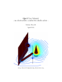
1
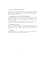
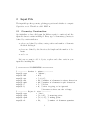
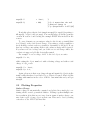
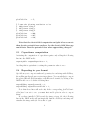
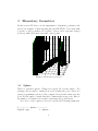
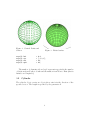
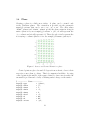
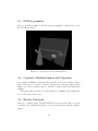
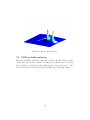
Qsci User Manual - an electrostatic conductive shells solver Stefano Boccelli April 2015 http://boccelliengineering.altervista.org Hi everybody! Qsci is a MATLAB script that compute the electrostatic field generated by conductive bodies. You can place spheres, cones, wires, planes, cylinders in the space, impose a voltage on them or let them float and impose an electric charge value; Qsci computes and plots the electric potential and electric field on planes, the charge density over the shells and capacities between conductors. Qsci may export Electric field, Potential and the geometry in POVray format. Qsci is under LGPLv3 license. Hope you enjoy! i Contents 1 Introduction 1 2 Input File 2.1 Geometry Construction . . 2.2 Plotting Properties . . . . 2.3 Capacitance computation . 2.4 Exporting in .pov format . . . . . 3 3 4 6 6 . . . . . . . 8 8 9 10 12 13 13 14 . . . . 3 Elementary Geometries 3.1 Sphere . . . . . . . . . . . . 3.2 Cylinder . . . . . . . . . . . 3.3 Cone . . . . . . . . . . . . . 3.4 Plane . . . . . . . . . . . . . 3.5 Line . . . . . . . . . . . . . 3.6 Wire Loop . . . . . . . . . . 3.7 Creating your own geometry . . . . . . . . . . . . . . . . . . . . . . . . . . . . . . . . . . . . . . . . . . . . . . . . . . . . . . . . . . . . . . . . . . . . . . . . . . . . . . . . . . . . . . . . . . . . . . . . . . . . . . . . . . . . . . . . . . . . . . . . . . . . . . . . . . . . . . . . . . . . . . . . . . . . . . . . . . . . . . . . . . . . . . . . . . . . . . . . . . . . . . . . . . . . . . . . . . . . . . 4 Numerical Method 16 4.1 Lumped Charges Method . . . . . . . . . . . . . . . . . . . . . 16 4.2 Capacity computation . . . . . . . . . . . . . . . . . . . . . . 17 5 Examples 5.1 Melting Pot . . . . . . . . . . . . . . . . . 5.2 Sharp Edge Effect . . . . . . . . . . . . . . 5.3 POVray geometry . . . . . . . . . . . . . . 5.4 Capacity of Isolated Sphere and Capacitor 5.5 Electric Field plot . . . . . . . . . . . . . . 5.6 POVray fields rendering . . . . . . . . . . ii . . . . . . . . . . . . . . . . . . . . . . . . . . . . . . . . . . . . . . . . . . . . . . . . . . . . . . . . . . . . . . . . . . 18 18 21 22 22 22 23 1 Introduction Well.. the first time I’ve been studying electromagnetism, I found a little weird that surface charge could eventually be non-uniformly distributed on a conducting surface. Of course, after some time and a little more knowledge it turned out to be a “why on Earth should it be otherwise??”, but still I find fascinating to watch at charge distribution, induced by other bodies.. and seeing how merging a floating voltage conductor into an electrostatic field can deflect the field lines to make its iso-potential dream true. Qsci was essentially born to quench this need for plotting. Since it didn’t want to be just a fashion tool, Qsci outputs the total charge and Voltage on every conductor. Qsci allows you to create some conductive shells or bodies via geometrycreating functions. You can assign to the surfaces a value for the electric potential or leave them floating and assign a total charge value, and Qsci calculates: • charge density on the surfaces (by default) • intensity of electric potential (on request) • electric potential (on request) • capacities between objects The electric field and potential are computed and plotted on three orthogonal planes. Also Qsci may export the fields and geometry to POVray .pov format. Geometry creation, plotting and exporting requests are managed through an input file called INPUT.m Which geometries can I create? At the moment, I’ve implemented spheres, planes, cones, cylinders, straight wires and loops. The firsts are surfaces and Qsci will output a surface density plot for them, while the latters are 1D elements and you will not see a linear density plot. You can implement your own geometry, see the appropriate chapter of this user manual. I’d really love to implement a cow or a cactus-like surface, so if someone would kindly implement that for me, I’d include him/her in the thanks to section! 1 What about the numerical magic? I really love lumped parameters methods: they are so intuitive and quickly implemented! Qsci disposes sources (electric charges) on the surfaces or lines and calculates the potential field in some control points. A linear system is solved and solution is served! Measuring Units - PAY ATTENTION HERE!!! Qsci works in IS units, but please be aware that to avoid working with values of 1E-12, every value for the charge is actually q/0 !!! That is, if you set a charge Q̃ = 20 units, you are actually setting a physical charge value of q = Q̃0 = 200 [C] ! Computed Capacities are typically huge: it’s because of the choice of not dividing by 0 . To obtain real capacities, multiply the output by 0 . What does Qsci mean? Since it was conceived as a script to plot surface charge distribution in electrostatics, “Qsci” is the contraction of Q, the universal symbol for charge and gusci, Italian word for “shells”. “Qsci” and “gusci” sound almost the same!! :) Licensing Qsci is a weekend project: I wouldn’t rely too much on Qsci results if I were you! Qsci is Open Source and is under LGPL license v3. 2 2 Input File The input file specifies geometry, plotting properties and whether to compute Capacities or not. This file is called INPUT.m. 2.1 Geometry Construction Qsci initializes a class called sups (in Italian superfici = surfaces) and the input file almost consists in filling it. Every type of elementary geometry is defined by certain attributes: • spheres are defined by radius, center position and number of elements in which dividing it. • planes are defined by the direction, the length and the number of elements • and so on Let’s say we want to add 2 objects, a sphere and a line: write in your input file something like % ============ MY CONDUCTORS ============ % ---------- Surface 1: sphere ---------sups(1).type = ’sphere’; sups(1).Rad = 0.6; sups(1).xyz = [-1,2,1]; sups(1).nth = 20; % number of elements in theta direction sups(1).nphi = 40; % number of elements in phi direction sups(1).V = 5; % Volts sups(1).Q = 0; % this is going to be ignored % because we have set the voltage % ---------- Object 2: wire ---------sups(2).type = ’line’; sups(2).xyzA = [2,-2,4]; % starting point sups(2).xyzB = [2,-2,-3]; % ending point sups(2).nL = 50; % number of elements spanwise 3 sups(2).V sups(2).Q = ’free’; = 300; % % Q = 3 means that the real % phisical charge is % q = Q*epsilon0 = 2.655 [nC] Don’t skip places, that is don’t jump from sups(1) to sups(3) forgetting to fill sups(2), or Qsci could get angry. You can find more about the geometry creation in section 3 and reading the example INPUT files included in the sources. To every element you can assign a value for the electric potential (that is a Voltage) or the total electric charge. Not setting a voltage results in a freely floating conductor whose potential is determined by the field. If you have set a voltage, any setting on the total conductor charge will be ignored. If you have not set a voltage and you didn’t set a total charge either, the conductor is supposed globally electrically neutral. For example: to set a voltage of 21V to the 3rd object, we write: sups(3).V = 21; while setting the object number 3 with a floating voltage and with a total charge of 3.4/0 reads: sups(3).V = ’free’; sups(3).Q = 3.4; Again, please note that every charge shown and inputted to Qsci is in the truth a value that have been divided by 0 . This is because I didn’t feel like working with numbers in the order of 1E-12. Just mind this and you’ll get straight. 2.2 Plotting Properties Surface Charge Surface charge is automatically computed and plotted in a single plot containing all the created geometrical entities. Plotting together multiple surfaces results in plots that are not very clear in terms of surface charge: you may desire a plot of some object on their own. This can be done by setting somewhere in the INPUT file lines like: 4 sups(4).plot_me_alone = 1; this will result in the production of a surface density plot for the object number 4. Note that surface density is implemented only for surface-like objects: setting plot me alone = 1 for a line object results in a plot of a completely black (and meaningless) line. Electrostatic field and Electrostatic Potential In order to plot the electrostatic field or the potential, you have to ask Qsci to do so. Qsci will show the fields on three planes merged in the volume and oriented as xy, yz and xz. First of all, tell Qsci that you want him to compute Potential and/or Electrostatic field, by writing the following in the INPUT file: plotField.plotPotential = 1; plotField.plotElectricField = 1; plotField.plotPotential enables a contour plot of the Electric Potential over planes. plotField.plotElectricField enables both a contour plot for the intensity of the the Electric field and also three cool surface plots. Not setting one of those variable is the same as setting them to zero. Then you must specify how long and where you want plot planes to be. In the INPUT file, set: % Put the intersection of the 3 planes in [-4,2,-1] plotField.xorig = -4; plotField.yorig = 2; plotField.zorig = -1; % % % % % The x coordinate must go from the origin (x=-4) ahead for Lx = 10 meters. The y coordinate must go from the origin (y=2), backwards for Ly = -10 meters The z coordinate starting from -1 forward for 5 m plotField.Lx plotField.Ly = 10; = -10; 5 plotField.Lz = -5; % I want the plotting resolution to be: % 100 points along x % 105 points along y % 130 points along x plotField.nx = 100; plotField.ny = 105; plotField.nz = 130; Note that the electric field computation and plot is less accurate than electric potential near surfaces, for the electric field blows up much faster than the potential does when approaching charges!! 2.3 Capacitance computation Activating the computation of capacities requires only adding the following line into the INPUT.m file: capacityCalc.computeCapacities = 1; Avoiding this is equivalent to setting the parameter value to zero. 2.4 Exporting in .pov format Qsci allows you to export results and geometry for renderings with POVray, the well known Open Source ray-tracing software. You can ask Qsci to export the plotted Electric Field intensity or the Electric Potential, by adding to the INPUT.m file one or both the following lines. exportPOVray.exportPotential = 1; exportPOVray.exportElectricField = 1; Note that those lines will work only if the corresponding plotField variables have been set to one: you must first enable plots in order to export them! If you have installed POVray and the image viewer feh, the following line in the INPUT.m file will automatically launch a POVray rendering and visualize the image with feh. Press Esc to quit. 6 exportPOVray.showMeResults = 1; PS: I’m not sure whether feh is available under Windows or not. In the Examples section, you can see the potential and electric field generated by a sphere and rendered with the exported POVray file. The exported file stores grid points and values for the solution on such points. Note that exported points are rescaled so that the biggest axis have a unitary length and the other axis is scaled accordingly. The solution is both rescaled and traslated: as a result, solution in POVray plot always goes from 0 to 1. This is simply to obtain a nice plot in many different situations.. To export the geometry, add in the INPUT.m file the following line: exportPOVray.exportGeo = 1; To modify camera, light, shining and color settings, you must modify a few parameters in the POVray geo export.m file. 7 3 Elementary Geometries In this section I’ll show you the implemented elementary geometries and provide an example of their inserting into the INPUT file. Let’s start with a picture of the geometries all together! Green circles represent charges (sources), while black stars represent control points. 4 3 2 Z 1 5 4 0 3 2 −1 1 0 −1 Figure 1: Elementary geometries 3.1 Sphere This is a generated sphere. Charges are spread all over the surface. For plotting reasons, surface density plots avoid plotting the poles: this is for purely programming reasons, for the computed area was inaccurate near the poles and the surface density thus had a numerically wrong peak. Exceed the number of elements if you want to investigate the polar regions. In order to create a sphere you need to specify the following parameters: % ---------- Sphere ---------sups(1).type = ’sphere’; 8 Figure 2: Control Points and Sources sups(1).Rad sups(1).xyz sups(1).nth sups(1).nphi = = = = Figure 3: Plotted surface 0.6; [-1,2,1]; 20; 40; The number of elements nth and nphi represent respectively the number of divisions from North to South and the number from West to East (that is latitude and longitude). 3.2 Cylinder The cylinder object creates an object whose axis is in the direction of the specified vector. The length is specified by the parameter L. 9 Figure 4: Sources and Control Points for the cylinder You create a cylinder by (here I gave it the number 2 but it’s arbitrary): % ---------- Cylinder ---------sups(2).type = ’cylinder’; sups(2).Rad = 0.3; % sups(2).Len = 6; % sups(2).xyz = [0,-2,-1]; % sups(2).nth = 10; % sups(2).nh = 40; % sups(2).vers = [0.7,2,0]; % 3.3 Radius Length Origin (mid point) # of angular divisions # of length divisions axis direction Cone Cones are pretty simple shapes for they have coarse grid at the base and very fine grid near the tip. The implemented cones are always truncated. If you want a sharp edge, you choose a very thin top radius. 10 Figure 5: Sources and Control Points for a sharp edge cone A cone is created by (here I choosed the number 4 but it’s arbitrary): % ---------- Surface 4 ---------sups(4).type = ’cone’; sups(4).Rbase = 0.7; sups(4).Rtop = 0.01; sups(4).Len = 4; sups(4).xyz = [2,1.5,0]; sups(4).nth = 20; sups(4).nh = 80; sups(4).vers = [0,0,1]; 11 % % % % % % % bottom radius radius for top length = height origin of the mid-height point # of angular divisions # of height divisions Axis direction 3.4 Plane Creating a plane is a little more tricky. A plane can be oriented only as the Cartesian planes. The orientation is specified via the parameter sups(jj).orient, that can be set to ‘xy’, ‘yz’ or ‘xz’. The other values ‘x1min’, ‘x1max’ and ’x2min’, ‘x2max’ specify the plane extension along its surface (that is if you set sups(jj).orient = ’yz’, x1 will represent the ‘y’ coordinate and x2 will represent ‘z’). Then, the vale ‘x3val’ represent the not varying coordinate (that is ‘x’ in our example). If unsure, just try it. Figure 6: Sources and Control Points for a plane Control points are placed around 45 degrees from each axis, closer to their respective source than to others. That’s for numerical stability: choosing control points in the middle of the square defined by four sources resulted in an unstable problem and a badly oscillating surface charge on the surface. % ---------- Plane ---------sups(3).type = ’plane’; sups(3).x1min = -5; sups(3).x1max = 5; sups(3).x2min = -3; sups(3).x2max = 4; sups(3).x3val = -2; sups(3).n1 = 60; sups(3).n2 = 40; sups(3).orient = ’yz’; 12 sups(3).d_cc = 0.02; This create a plane where ‘y’ goes from -5 to 5, ‘z’ from -3 to 4 and ‘x’ has the value -2. 3.5 Line Line objects are straightforward: A is the starting point and B the end. Figure 7: This is how a straight line looks like % ---------- Line ---------sups(5).type = ’line’; sups(5).xyzA = [2,-2,4]; % starting point sups(5).xyzB = [2,-2,-3]; % ending point sups(5).nL = 50; 3.6 Wire Loop Here are input parameters for a wire loop. 13 −0.5 −1 −1.5 −4 −3.5 2 −3 2.5 3 −2.5 −2 3.5 4 Figure 8: Wire Loop % ---------- Wire Loop ---------sups(6).type = ’loop’; sups(6).Rad = 1; sups(6).xyz = [3,-3,-1]; sups(6).nth = 50; sups(6).vers = [0,1,1]; 3.7 % % % % loop radius loop center number of elements orientation versor Creating your own geometry To create your own geometry, you have to write down a function returning: 1. position rq for sources, dimension Npoints ∗ 3 2. position rc for control points, dimension Npoints ∗ 3 3. matrices xxc, yyc, zzc of control points positions in meshgrid format (they will be used to plot surfaces) 4. matrix of element area Amat (or length Lmat for line elements) in the same format as xxc You can call this function something like my own geometry creator.m and modify the geometry creator.m file in order to take it into account. 14 Also, if you want a surface charge plot you have to create another function that reshapes the vector of charges generated by the solver, matching the same meshgrid format as xxc, yyc, zzc, Amat.. The dirty way - a hint There’s actually another way: if you are not interested in plotting the surface, you could simply add a surface from the input file and give it a type attribute: sups().type = ’666’. This will result in an unknown surface and thus will probably not generate errors. Then you must assign values for the sources and control points position to rq and rc attributes of your surface. Maybe you could write a little script to fill sups().rq and rc and place it in the MAIN.m file, right after the INPUT calling. The method should result in a conductor that is invisible in surface plots, but that affects the field: contour planes should be alright. Haven’t tried this out anyway. 15 4 4.1 Numerical Method Lumped Charges Method A brief overview of the numerical method. The underlying idea of the method is: “a conductor is an equipotential body, right? So, let’s place a number of charges on every conducting surface and then impose that the electric potential generated by all the charges on the control points of a the same surface be the same” Let’s place ourselves on the ith control point. The electric potential induced by all the charges follows the principle: superposition q1 q2 1 1 1 1 1 Vi = 4π0 r1i r2i r3i ... rN i q3 ... qN where rji represents the distance between the j th source and the ith control point. Now, if the control point belongs to an object whose potential was imposed (through the input file), then Vi is a known value, otherwise the voltage Vi will will be kept as unknown. Conductors whose voltage is not set require an additional condition, that is the value for total charge. This constraint for the k th body reads: k q1 q2k k k 1 1 1 ... 1 q3 = Q ... k qN k A C q Vimposed where We end up with a system in the form: = D 0 V Qimposed 1 1 A stores the influence coefficients 4π , C multiplies floating (and thus un0 rji known) potentials, D is made of ones for charges relative to floating potentials (and thus imposed total charge), picking only the charges belonging to the k th body and b is the right hand (known) term. NOTE THAT since I didn’t like to have a matrix storing values ranging from 1E12 (that is 1/0 ) to unitary values, I lumped the 0 coefficient into the charges value. In the input file you must enter a value that is the real physical charge you want to impose, divided by 0 ! 16 4.2 Capacity computation First of all note that Capacity computation may be quite expensive, for Qsci must solve the linear system N times, where N is the number of objects. Computing the capacity of our object is achieved by computing the so called elastance matrix, followed by it’s inversion and one last little step. Let’s say we have three objects with total charges q1 , q2 , q3 . We can write: V1 = s11 q1 + s12 q2 + s13 q3 V2 = s21 q1 + s22 q2 + s23 q3 V3 = s31 q1 + s32 q2 + s33 q3 that is: s11 s12 s13 q1 V1 V2 = s21 s22 s23 q2 V3 s31 s32 s33 q3 To compute the elastance matrix s, Qsci puts a unitary charge on a surface, null charge on the others and computes induced potentials. After finding s, Qsci inverts it: s = s−1 . This is called capacitance matrix. Then, Capacities are readily found: f or i 6= j Cij = −cij ,X Cij Cii = cii − j6=i The coefficients Cii represent the capacity of the ith object with respect to a reference huge sphere at the borders of the universe, while the coefficients Cij are the capacity of the capacitor made by the ith and j th objects. A Capacity matrix made with those capacities is displayed in the command window. Remember what I said about q and 0 ? The capacities must be multiplied by 0 in order to obtain the real physical value! 17 5 Examples In this section some colored plots!!! 5.1 Melting Pot Here’s a simulation of a melting pot of the objects that Qsci implements. Object Imposed Voltage [V] sphere 5 cylinder free free plane cone -10 0 line Resulting Voltage [V] -1.395 -0.034 - Table 1: Imposed and simulated electric potentials for objects. Figure 9: Charge density distribution on the plane Figure 10: Charge density distribution around the edge of the cone 18 Figure 11: Charge density distribution on the cylinder Figure 12: Charge density distribution upon the sphere Figure 13: Eletctostatic 19potential contour lines. Figure 14: Sources and control points. 20 5.2 Sharp Edge Effect Here’s a nice pic about the intensification of charge density around sharp corners! Figure 15: Charge density around a sharp edge. 21 5.3 POVray geometry Here’s a geometry, similar to the the previous example’s, exported in a .pov file and then rendered. Figure 16: A geometry rendered with POVray. 5.4 Capacity of Isolated Sphere and Capacitor As a quick benchmark, I calculated the capacity of an isolated sphere, whose value is known to be 4πR0 by theory. I’m proud to announce that on this simple case, Qsci’s result is exact to the 0.6%, with around 200 distributed charges! The plane plates capacitor is a little harder to simulate and results vary a lot.. 20% may be the case! 5.5 Electric Field plot Here’s a cool shaded plot of the Electric Field intensity near a wire loop and a cylinder. Note that the field tries to blow up near the wire and the cylinder surface! 22 Figure 17: Electric Field intensity. 5.6 POVray fields rendering This how a POVray rendering of the exported file looks like. Theese are the electric field and electric potential of a spherical conductive shell. Note that the potential is constant along the shell and the electric field is zero. Also note how faster the electric field blows up while approaching the surface! 23 Figure 18: Electric Potential of a sphere. Figure 19: Electric Field of a sphere. The sphere has 30 lumped charges distributed in equatorial direction. 24