Download The NIRISS Wide-Field Slitless Spectroscopy Cookbook

JWST-STScI-002949, SM-12
Revision -
Space Telescope Science Institute
JAMES WEBB SPACE TELESCOPE MISSION
SCIENCE AND OPERATIONS CENTER
The NIRISS Wide-Field Slitless Spectroscopy Cookbook
An Informal Guide to Data Simulation and Analysis
Technical Report
Revision Date: 11 December 2012
Operated by the Association of Universities for Research in Astronomy, Inc., for the National Aeronautics
and Space Administration under Contract NAS5-03127
Check with the JWST SOCCER Database at: https://soccer.stsci.edu
To verify that this is the current version.
NIRISS Wide-Field Spectroscopy Cookbook
JWST Mission Science & Operations Center
JWST-STScI-002949, SM-12
Revision -
CM Foreword
This document is an STScI JWST Configuration Management-controlled document. Changes to
this document require prior approval of the STScI JWST CCB. Proposed changes should be
submitted to the JWST Office of Configuration Management.
ii
Check with the JWST SOCCER Database at: https://soccer.stsci.edu
To verify that this is the current version.
NIRISS Wide-Field Spectroscopy Cookbook
JWST Mission Science & Operations Center
JWST-STScI-002949, SM-12
Revision -
Signature Page
Prepared by:
Electronic Signature
William Van Dyke Dixon
NIRISS Instrument Scientist
STScI/INS
6/18/2012
Reviewed by:
Alex Fullerton
NIRISS Branch Manager
STScI/INS
7/6/12
Tom Brown
7/6/12
WBS Manager
STScI/JWST Mission Office
Approved by:
David Hunter
Project Manager
STScI/JWST Mission Office
12/11/12
iii
Check with the JWST SOCCER Database at: https://soccer.stsci.edu
To verify that this is the current version.
NIRISS Wide-Field Spectroscopy Cookbook
JWST Mission Science & Operations Center
JWST-STScI-002949, SM-12
Revision -
STScI JWST Document Change Record
Title: NIRISS Wide-Field Spectroscopy Cookbook
STScI JWST CI No: JWST-STScI-002949
Change No./Date
Description of Change
Revision: Change Authorization/Release:
JWST-STScI-CR-002972
Baseline
CCB 12/11/12 (out-of-board)
iv
Check with the JWST SOCCER Database at: https://soccer.stsci.edu
To verify that this is the current version.
NIRISS Wide-Field Spectroscopy Cookbook
JWST Mission Science & Operations Center
JWST-STScI-002949, SM-12
Revision -
Table of Contents
1
2
3
4
5
6
7
Introduction ............................................................................................................................ 1-1
1.1 The Software ................................................................................................................... 1-1
1.2 The Instrument ................................................................................................................ 1-1
1.3 What’s New .................................................................................................................... 1-2
1.4 Reference Documents ..................................................................................................... 1-2
Setting Up .............................................................................................................................. 2-1
2.1 Retrieve the Necessary Software and Configuration Files ............................................. 2-1
2.2 Configure Your Environment ......................................................................................... 2-1
Generate Synthetic Data ........................................................................................................ 3-1
3.1 Input Files Provided by the NIRISS Team ..................................................................... 3-1
3.2 Input Files Provided by the User .................................................................................... 3-2
3.2.1 Model Object Table ................................................................................................. 3-2
3.2.2 Template Spectra and Images .................................................................................. 3-4
3.2.3 Scaling Spectra and Images ..................................................................................... 3-4
3.3 Running aXeSIM ............................................................................................................ 3-5
3.4 aXeSIM Output ............................................................................................................... 3-5
3.5 Reference Documents ..................................................................................................... 3-7
Prepare Input Files for Spectral Extraction ............................................................................ 4-1
4.1 Copy and Modify Image Files ........................................................................................ 4-1
4.2 Use SExtractor to Construct New MOT ......................................................................... 4-1
4.3 Construct Input Image List ............................................................................................. 4-3
4.4 Move Files into Position ................................................................................................. 4-3
Extract Spectra from Dispersed Image .................................................................................. 5-1
5.1 Preparing the Spectral Extraction: axeprep..................................................................... 5-1
5.2 Extracting Individual Spectra: axecore ........................................................................... 5-1
5.3 Reference Documents ..................................................................................................... 5-1
Creating Web Pages to Review Your Results........................................................................ 6-1
6.1 Reference Documents ..................................................................................................... 6-3
Simulating Observations with GR150C................................................................................. 7-1
7.1 Rotate the Catalog and Any Template Images ............................................................... 7-1
7.2 Rotate the Image Header ................................................................................................. 7-1
7.3 Further Analysis .............................................................................................................. 7-2
7.4 Reference Documents ..................................................................................................... 7-2
v
Check with the JWST SOCCER Database at: https://soccer.stsci.edu
To verify that this is the current version.
NIRISS Wide-Field Spectroscopy Cookbook
JWST Mission Science & Operations Center
JWST-STScI-002949, SM-12
Revision -
List of Figures
Figure 3-1 Zero- and first-order spectra of the seven objects in our example. ............................ 3-6
Figure 4-1 Detail of apertures.fits showing that SExtractor has identified our spiral galaxy as five
separate objects. ................................................................................................................... 4-2
Figure 6-1 Output of aXe2web, showing the direct image, the two-dimensional spectrum, and the
extracted spectrum in both counts and flux units for each object in the catalog. ................ 6-2
Figure 7-1 Detail of rotate_slitless.fits showing the overlap of object spectra. ........................... 7-2
List of Tables
Table 1-1 Bandpass and Backgrounds for NIRISS Filters .......................................................... 1-2
vi
Check with the JWST SOCCER Database at: https://soccer.stsci.edu
To verify that this is the current version.
NIRISS Wide-Field Spectroscopy Cookbook
JWST Mission Science & Operations Center
1
JWST-STScI-002949, SM-12
Revision -
Introduction
1.1
The Software
The purpose of this document is to provide a brief introduction to the software available to model
wide-field slitless spectroscopic observations with NIRISS and to extract and calibrate the
resulting spectra. The tools employed are the aXe package of programs (Kümmel et al. 2009),
which was developed to support slitless spectroscopy with ACS and WFC3 on the Hubble Space
Telescope, and Source Extractor (a.k.a. SExtractor; Bertin & Arnouts 1996), which builds a
catalog of objects from an astronomical image.
The aXe package includes three tools: aXeSIM is used to generate synthetic direct and
dispersed images of the sky, aXe extracts and calibrates spectra, and aXe2web displays the
resulting data in a convenient HTML format. (The web-based tool aXeSIMweb is not discussed
in this document, as it currently simulates only WFC3 data.)
This cookbook follows closely the format of The WFC3 IR Grism Data Reduction Cookbook,
version 1.15 (Kuntschner et al. 2012). Other useful documents are The aXeSIM Manual, version
1.4 (Kümmel, Walsh, & Kuntschner 2010) and the aXe User Manual, version 2.3 (Kümmel et al.
2011). Source Extractor is described in the SExtractor User’s Manual, version 2.13 (Bertin
2009), and Source Extractor for Dummies (Holwerda 2005). All of these documents are
included in the compressed tar file discussed in Section 2. Note that the WFC3 cookbook is
subject to frequent revision. The most recent version is available from the WFC3 Spectroscopy
Resource Page.
1.2
The Instrument
The Near Infrared Imager and Slitless Spectrograph (NIRISS; Doyon et al. 2012) offers widefield slitless spectroscopy (WFSS) with a resolving power R = 150 over the wavelength range
1.0 to 2.25 μm using either of two orthogonal grisms, GR150C and GR150R. The grisms are
named such that GR150C disperses into detector columns (i.e., vertically) and GR150R disperses
into rows (horizontally). If the grisms were used without a filter, their first-order spectra would
overlap those of higher orders, and the sky background would be unacceptably high. Table 1-1
lists the five filters available for WFSS, their bandpasses, and the estimated count rates for
zodiacal and stray light in each filter. 1
NIRISS employs a single HgCdTe detector with 2048 × 2048 pixels, each 18 μm across. The
outer 4 pixels on each side are reference pixels, insensitive to light, so the active area is 2040 ×
2040 pixels. The field of view is 134” × 135”; each pixel thus spans 65.4 mas × 65.8 mas. For
simplicity, our models assume a plate scale of 64 mas/pixel.
For additional information about NIRISS, its capabilities, and modes of operation, see the
NIRISS Operations Concept Document (Goudfrooij et al. 2012) and the NIRISS OSIM Test Plan
(Martel 2012).
1
See “A note about backgrounds” at the end of this section.
1-1
Check with the JWST SOCCER Database at: https://soccer.stsci.edu
To verify that this is the current version.
NIRISS Wide-Field Spectroscopy Cookbook
JWST Mission Science & Operations Center
JWST-STScI-002949, SM-12
Revision -
Table 1-1 Bandpass and Backgrounds for NIRISS Filters
Filter
Name
Pivot
Bandpass
Zodiacal
Stray Light
Wavelength
(μm)
Light
(e–/s/pix)
–
(nm)
(e /s/pix)
F090W
901
0.8 – 1.0
0.42
0.50
F115W
1150
1.0 – 1.3
0.43
0.47
F140M
1406
1.3 – 1.5
0.21
0.23
F150W
1498
1.3 – 1.7
0.44
0.48
F158M
1583
1.5 – 1.7
0.22
0.25
F200W
1984
1.75 – 2.25
0.39
0.44
Count rates represent the combination of a GR150 grism and the listed blocking filter.
A note about backgrounds: For sensitivity calculations, the JWST project uses a zodiacal-light
spectrum scaled to 1.2 times its minimum intensity on the sky. Stray light refers to light from all
objects (zodiacal dust, stars, Earth, and Moon) more than 1° from the line of sight that is
scattered into the field of view by dust on the optics. Stray-light values are taken from Mission
Requirement 121 (MR-121; Bussman 2011), which limits stray light to 0.091 and 0.070 MJy/sr
at wavelengths of 2.0 and 3.0 μm, respectively. The dark current of the NIRISS detector adds an
additional 0.015 e–/s to each pixel. The read noise is roughly 6 e–/pixel for a 1 ks exposure
(assuming the standard NIRISS observing mode).
A note about F090W: At wavelengths between 0.8 and 0.9 μm, representing half of the
F090W bandpass, the throughput of the GR150 grisms is higher in second order than in first.
1.3
What’s New
The WFC3 cookbook begins with the reduction of an archival data set, then demonstrates the
utility of aXeSIM in interpreting the resulting spectra. Lacking archival data for NIRISS, we
begin by using aXeSIM to create a pair of direct and dispersed images (Sections 2 and 3), then
use Source Extractor and aXe to identify the sources (Section 4) and extract their spectra
(Section 5). We display the resulting spectra in an HTML format using aXe2web (Section 6).
Because the aXe software can neither model nor extract spectra dispersed vertically on the
detector, we provide instructions for simulating observations with grism GR150C (Section 7).
We do not discuss the use of multidrizzle and axedrizzle to combine data from multiple
exposures.
The aXe software package, along with our understanding of the NIRISS instrument and its
operating modes, will evolve significantly in the years leading up to the launch of JWST. This
document and the associated NIRISS configuration and calibration files will be revised as
necessary to reflect these developments.
1.4
Reference Documents
Bertin, E. 2009, SExtractor User’s Manual, Version 2.13
Bertin, E. & Arnouts, S. 1996, Astronomy & Astrophysics Supplement, 317, 393
Bussman, M. 2011, “JWST Mission Requirements Document,” JWST-RQMT-000634, Rev. AD
1-2
Check with the JWST SOCCER Database at: https://soccer.stsci.edu
To verify that this is the current version.
NIRISS Wide-Field Spectroscopy Cookbook
JWST Mission Science & Operations Center
JWST-STScI-002949, SM-12
Revision -
Doyon, R., et al. 2012, in Space Telescopes and Instrumentation 2012: Optical, Infrared, and
Millimeter Wave Conference, Proceedings of SPIE Vol. 8442
Goudfrooij, P., et al. 2012, “NIRISS Operations Concept Document,” in preparation
Holwerda, B. W. 2005, Source Extractor for Dummies
Kuntschner, H., Kümmel, M., Walsh, J. R., & Lee, J. C. 2012, The WFC3 IR Grism Data
Reduction Cookbook, Version 1.15
Kümmel, M., Walsh, J. R., & Kuntschner, H. 2010, The aXe SIMulation Package aXeSIM: User
Manual, Version 1.4
Kümmel, M., Walsh, J. R., Kuntschner, H., & Bushouse, H. 2011, aXe User Manual, Version 2.3
Kümmel, M., Walsh, J. R., Pirzkal, N., Kuntschner, H., & Pasquali, A.J. 2009, PASP, 121, 59
Martel, A. 2012, “OSIM Test Plan for
”
NCSA‐
IRISS,JWST‐ PL‐ 0012
1-3
Check with the JWST SOCCER Database at: https://soccer.stsci.edu
To verify that this is the current version.
NIRISS Wide-Field Spectroscopy Cookbook
JWST Mission Science & Operations Center
2
2.1
JWST-STScI-002949, SM-12
Revision -
Setting Up
Retrieve the Necessary Software and Configuration Files
Both aXe and aXeSIM are included in the PyRAF/IRAF package STSDAS. If this package is
not available on your computer, the aXe software and its associated documentation can be
retrieved from the aXe website. The program aXe2web is not included in STSDAS, so must be
installed by hand. (Here is a direct link to the aXe distribution page.) The code and
documentation for Source Extractor are available from Astromatic.net.
The aXe programs require a number of calibration and configuration files, and they read and
write files into a particular set of subdirectories. All are available as a single compressed tar file
on the NIRISS web site. Unpack this file in a convenient workspace. We will do all of our work
within the resulting directory, called “cookbook.” Its subdirectories are
CONF
Configuration and calibration files
DATA
Input files used by aXe
DOCUMENTATION
User manuals
DRIZZLE
Required but not used by aXe
OUTPUT
Output files generated by aXe
OUTSIM
Output files generated by aXeSIM
SAVE
A safe copy of the input files used by aXe
SCRIPTS
Shell and Python scripts used by this cookbook
SIMDATA
Input files used by aXeSIM
VISUALIZATION
aXe2web works in this directory
2.2
Configure Your Environment
Define the following environment variables in the appropriate configuration file (.login,
.mysetenv, .setenv, or equivalent):
# Environment Variables used by aXe
setenv AXE_CONFIG_PATH ./CONF
setenv AXE_DRIZZLE_PATH ./DRIZZLE
setenv AXE_IMAGE_PATH ./DATA
setenv AXE_OUTPUT_PATH ./OUTPUT
setenv AXE_OUTSIM_PATH ./OUTSIM
setenv AXE_SIMDATA_PATH ./SIMDATA
We have written a number of shell and Python scripts to save you some typing as you work
through this cookbook. To use them, execute the following commands from within the
cookbook directory:
> setenv PATH ${PWD}/SCRIPTS:${PATH}
> rehash
If you are working at STScI, follow the instructions at http://stsdas.stsci.edu/configuration.html
to install and/or configure the latest version of STSDAS on your machine. Enter the command
> ssbrel
2-1
Check with the JWST SOCCER Database at: https://soccer.stsci.edu
To verify that this is the current version.
NIRISS Wide-Field Spectroscopy Cookbook
JWST Mission Science & Operations Center
JWST-STScI-002949, SM-12
Revision -
each time that you begin a session with this cookbook. Note that aXe2web (discussed in Section
6) is not installed on the STScI computers by default. You might want to go ahead and install it
now.
2-2
Check with the JWST SOCCER Database at: https://soccer.stsci.edu
To verify that this is the current version.
NIRISS Wide-Field Spectroscopy Cookbook
JWST Mission Science & Operations Center
3
JWST-STScI-002949, SM-12
Revision -
Generate Synthetic Data
We begin by generating a pair of direct and dispersed images using aXeSIM. For this exercise,
we consider only the F150W filter, but any of the other filters may be used.
3.1
Input Files Provided by the NIRISS Team
Both aXe and aXeSIM employ a suite of configuration and calibration files, most of which may
be found in the CONF directory. A brief description of each file follows. Separate
configuration, throughput, and sensitivity files are provided for each filter; the examples below
are for F150W. Eventually, we will have a complete set of files for each grism; for the moment,
we use one set of files for both.
NIRISS.F150W.conf – The configuration file, in ASCII format, describes the offset of each
spectral order from the source in the direct image, the shape of the trace (i.e., the variation in Y
as a function of X), and the dispersion solution of each order. All of these parameters may vary
across the field of view. Once NIRISS is launched, we will measure them for each combination
of grism and filter. For now, we model the position of each order, assuming that the offset is
independent of detector position, the trace is constant in Y, and the dispersion is linear. The file
also lists various instrument parameters, including the detector gain and read noise. The entry
for the gain is commented out as a reminder that the aXe package works with images in units of
e–/s.
NIRISS.F150W.tpass.V0.fits – The throughput files are used to construct direct images
of the field. They are FITS-format binary tables with two columns, wavelength and throughput.
Wavelength is in Ångstroms, and throughput is a real number between 0 and 1. The throughput
multiplied by the area of the telescope yields the instrumental effective area at each wavelength,
so the throughput includes everything from the shading by the secondary mirror to the detector
quantum efficiency. Because this file is used only by aXeSIM, it lives not in the CONF
directory but in SIMDATA.
NIRISS.F150W.1st.sens.V0.fits – The sensitivity files are used to construct spectra.
The sensitivity is the product of the instrumental effective area (computed above) and the grism
throughput, divided by the conversion from ergs to photons. The files are FITS-format binary
tables with three columns: wavelength, sensitivity, and error. Wavelength is in Ångstroms, and
both sensitivity and error are in e–/s/Å per erg/cm2/s/Å. (Section 6.1 of the aXe User Manual
incorrectly states that the sensitivity is in e–/s per erg/cm2/s/Å.) At present, errors are simply 3%
of the sensitivity. Separate files are provided for orders -1 through 3, for a total of five per filter.
(In the example given here, “1st” refers to first order.)
NIRISS.GR150R.flat.V0.fits – This is not the flat-field file used in the standard JWST
calibration pipeline. The response function of a detector is generally wavelength dependent. In
slitless spectroscopy, a pixel can receive flux from any wavelength. Thus, aXe employs a
wavelength-dependent flat-field correction. As we presently have no information about the flat
field of the NIRISS detector, our flat field is simply a two-dimensional array of 1’s. Note that
aXeSIM ignores this file completely; any flat-field features must be added to the model images
by hand.
NIRISS.GR150R.sky.V0.fits – When global subtraction of a master sky image is
requested, aXe identifies uncontaminated regions on the detector, determines the mean level in
3-1
Check with the JWST SOCCER Database at: https://soccer.stsci.edu
To verify that this is the current version.
NIRISS Wide-Field Spectroscopy Cookbook
JWST Mission Science & Operations Center
JWST-STScI-002949, SM-12
Revision -
those regions, and scales the master sky image to match that mean. Once NIRISS is launched,
we will construct a master sky image by combining grism images from multiple science
programs, masking the object spectra in each. In the mean time, we assume that the background
is uniform; our sky image is an array of 1’s.
We won’t actually feed the master sky image to aXeSIM. Instead, we will instruct the program
to use a uniform background. Note that aXeSIM ignores dark current; any detector background
must be included in the master sky image or added to the model images by hand.
3.2
Input Files Provided by the User
The aXeSIM Manual provides four examples of simulations with varying degrees of complexity.
Here we provide a single example, but include a variety of input options.
3.2.1
Model Object Table
The model is controlled by the model object table (MOT), which describes the coordinates,
magnitude, and shapes of all objects in the field. The MOT is an ASCII file in the form of a
SExtractor output catalog; its format is fully detailed in Section 1.2 of The aXeSIM Manual. It
lives in the DATA directory. Our MOT is called example.cat:
#
#
#
#
#
#
1
2
3
4
5
6
NUMBER
X_IMAGE
Y_IMAGE
A_IMAGE
B_IMAGE
THETA_IMAGE
Object number
X coordinate (pixels)
Y coordinate (pixels)
Length of semi-major axis (pixels)
Length of semi-minor axis (pixels)
Angle of major axis (counter-clockwise from +X axis)
#
#
#
#
7
8
9
10
1
2
3
4
5
6
7
MAG_F1537
SPECTEMP
Z
MODIMAGE
900.00
700.00
900.00
800.00
900.00
950.00
900.00 1050.00
900.00 1100.00
900.00 1150.00
900.00 1200.00
Magnitude at 1537 nm (WFC3 F160W)
Key to spectral template
Redshift
Key to model image
0.5
0.5
0.0 22.5 0 0.0
30.0 10.0 45.0 18.0 0 0.0
18.0 10.0 -30.0 18.0 1 0.0
5.0
2.0 60.0 18.0 2 0.0
5.0
2.0 60.0 18.0 2 0.075
5.0
2.0 60.0 18.0 2 0.15
5.0
2.0 60.0 18.0 2 0.22
0
0
1
0
0
0
0
The object number (column 1) is not terribly important to aXeSIM, but central to the
performance of aXe, as it is used to identify objects throughout the various stages of spectral
extraction and calibration.
For each object in the MOT, the user may either supply a template image or describe its shape
in terms of a 2-D Gaussian. If a template image is supplied, the object coordinates X_IMAGE
and Y_IMAGE (columns 2 and 3) represent the point to which the center of the template is
mapped. If a Gaussian is requested, they are the coordinates of the object centroid.
3-2
Check with the JWST SOCCER Database at: https://soccer.stsci.edu
To verify that this is the current version.
NIRISS Wide-Field Spectroscopy Cookbook
JWST Mission Science & Operations Center
JWST-STScI-002949, SM-12
Revision -
Columns 4, 5, and 6 list the object shape parameters. If a Gaussian is requested, then
A_IMAGE is the length of its semi-major axis, B_IMAGE is the length of its semi-minor axis,
and THETA_IMAGE is the angle between the major axis of the object and the X axis of the
image, measured counter clockwise. (A_IMAGE and B_IMAGE describe the width of a 2-D
Gaussian in the same way that σ does for a 1-D Gaussian.) These parameters should have
reasonable values even if a template image is supplied, as they are used by aXeSIM to perform a
toy extraction of the model spectrum.
Column 7 lists the total AB magnitude in one filter or at a particular wavelength. The column
name indicates the pivot wavelength of the filter or the wavelength at which the magnitude was
measured. In this case, MAG_F1537 corresponds to a wavelength of 1537 nm, the pivot
wavelength of the WFC3 F160W filter, through which (we will pretend) these galaxies have
been observed. Any number of magnitudes may be specified. How they are used depends on
whether a template spectrum is supplied.
If no template spectrum is supplied (the value in column 8 is 0), then a single magnitude value
will result in an object spectrum that is constant in fλ. Given two or more magnitudes, the
program will interpolate linearly between them. At wavelengths beyond those of the listed
magnitudes, the object spectrum is flat (i.e., constant in fλ).
If a template spectrum is supplied (the value in column 8 is greater than 0; see Section 3.2.2), it
is first redshifted, then rescaled to match the magnitude given in the MOT. In the current
example, object #3 has magAB = 18.0 at 1537 nm, which corresponds to a flux density of 3×10-17
erg/cm2/s/Å. The template spectrum will be averaged over the interval tpass_flux (specified
on the command line) and rescaled to have a mean flux density of 3×10-17 erg/cm2/s/Å in that
interval. The range of tpass_flux should match that of the magnitude given in the MOT. In
our example, magnitudes were measured though the WFC3 F160W filter, which has a bandpass
of 1400 to 1700 nm, so we set tpass_flux = '1400,1700'. If the wavelength of the input
magnitude lies outside of tpass_flux, then the spectral scaling will probably be incorrect, but
aXeSIM will not complain. If more than one magnitude is provided, the value closest to the
pivot wavelength of tpass_flux is used. It is an error if the redshifted template spectrum does
not span the wavelength interval tpass_flux.
This scaling algorithm can have a surprising effect: Two otherwise identical spectra will be
scaled by wildly different factors if one has a strong emission feature within tpass_flux and
the other does not.
If the requested redshift (column 9) is greater than zero, then the template spectrum is
redshifted as described above. If the template spectrum is already redshifted, then you should set
the value in the REDSHIFT column to zero. If no template spectrum is supplied, then the
redshift is ignored.
If a template image is supplied (the value in column 10 is greater than 0; see Section 3.2.2),
then the template image is centered on the point (X_IMAGE, Y_IMAGE) and dropped pixel-forpixel onto the output image of the field. If X_IMAGE and Y_IMAGE are not integers, then the
image is appropriately resampled. The user must apply any necessary convolution, shift,
rotation, or spatial scaling of the template image before running aXeSIM. In particular, aXeSIM
ignores all WCS information in the template-image header. If no template image is supplied (the
3-3
Check with the JWST SOCCER Database at: https://soccer.stsci.edu
To verify that this is the current version.
NIRISS Wide-Field Spectroscopy Cookbook
JWST Mission Science & Operations Center
JWST-STScI-002949, SM-12
Revision -
value in column 10 is 0), then a 2-D Gaussian described by the parameters A_IMAGE,
B_IMAGE, and THETA_IMAGE is centered at the coordinates (X_IMAGE, Y_IMAGE).
Note that these columns may appear in any order, as long as they are properly labeled in the
MOT header. Additional columns may be present, but they will be ignored by aXeSIM.
Now let us consider the seven objects in the MOT:
Object 1 is a star and thus unresolved. At 1.5 μm, the FWHM of the instrumental PSF is about
1.2 pixels, so we set both A_IMAGE and B_IMAGE = 0.5. The stellar magnitude is 22.5; the
resulting spectrum will be flat in fλ. We ignore the spectral and image templates by setting them
to zero.
Object 2 uses a 2-D Gaussian to construct an image of an elliptical galaxy. The requested
values of A_IMAGE, B_IMAGE, and THETA_IMAGE will produce an ellipse with a semimajor axis of 30 pixels, a semi-minor axis of 10 pixels, and a rotation angle of 45°.
Object 3 is a spiral galaxy. Here we employ both a template image (#1) and a template
spectrum (#1). The template image has been convolved with the NIRISS PSF.
Finally, objects 4 through 9 are small galaxies, described with Gaussians, all using the same
template spectrum (#2) but at a variety of redshifts. The spectrum is identical to that of object 3,
but with a strong emission feature at 1.35 μm; this line will march across the F150W bandpass as
the redshift increases.
3.2.2
Template Spectra and Images
Both object spectra and images can be supplied via external files. Spectra may be either ASCII
or binary FITS files containing two columns, the wavelength in Ångstroms and the flux density
in erg/cm2/s/Å. The wavelength must increase monotonically. Images must be stored in FITS
files with at most two extensions. If the file has two extensions, the first extension (i.e., the
primary HDU) must be empty and the second must contain the data. The files are stored in the
SIMDATA directory.
Lists of the template spectral and image files, here called template_spectra.txt and
template_images.txt, are provided in the main directory. The names of these lists are provided to
aXeSIM on the command line. The key used by the MOT to select a template from either list is
simply the line number of the file in that list (beginning with line 1). If no template is desired,
the key should be set to zero.
3.2.3
Scaling Spectra and Images
The spectrum of each object in the MOT is scaled according to the algorithm described in
Section 3.2.1. To make the dispersed image, that spectrum is converted from physical units into
e–/s using the sensitivity files for each order. At each wavelength step, a copy of the object
image is scaled to the appropriate intensity and dropped onto the output array. To make the
direct image, the spectrum is scaled by the effective-area curve (the product of the telescope area
and the throughput curve for the desired filter) and converted to units of e–/s. A copy of the
object image is then scaled and dropped onto the output array. Note that we have used input
parameters (magnitudes and bandpass) for the WFC3 F160W filter, but output parameters
(sensitivity and throughput curves) for the NIRISS F150W filter. The result is an (imaginary)
image obtained through the NIRISS F150W filter.
3-4
Check with the JWST SOCCER Database at: https://soccer.stsci.edu
To verify that this is the current version.
NIRISS Wide-Field Spectroscopy Cookbook
JWST Mission Science & Operations Center
3.3
JWST-STScI-002949, SM-12
Revision -
Running aXeSIM
Once the input files are in place, aXeSIM can be run directly from the command line using the
following python script:
> run_example.py
This script calls the program simdata with the following arguments:
simdata incat='example.cat' config='NIRISS.F150W.conf'
tpass_direct='NIRISS.F150W.tpass.V0.fits' tpass_flux='1400,1700'
inlist_spec='template_spectra.txt' inlist_ima='template_images.txt'
bck_flux_dir = 0.94 bck_flux_disp = 0.94
exptime_dir = 100 exptime_disp = 10000 extraction='YES'
nx_disp=2040 ny_disp=2040 nx_dir=2040 ny_dir=2040
The parameters on the first three lines have already been discussed. In the fourth line, a
uniform background is added to both the direct and dispersed images by setting the parameters
bck_flux_dir and bck_flux_disp to 0.94 e–/s, the sum of the zodiacal and scattered light
through the F150W filter (Table 1-1) and the dark current for the NIRISS detector. Either a
uniform background or a background image (in e–/s) can be added using these parameters.
Exposure times for the direct and dispersed images are set by specifying the parameters
exptime_dir and exptime_disp, respectively. aXeSIM scales the output image (sources
plus background) to the requested exposure time, adds Poisson noise (for both sources and
background) and read noise (from the configuration file), and divides by the exposure time to
produce an image with units of e–/s. While the EXPTIME keyword in the primary header will
reflect the requested exposure time, the image itself will always be in units of e–/s. If not
provided with an exposure time, aXeSIM produces a noise-free image in units of e–/s.
Note that the dispersed image has an exposure time of 10,000 seconds. In reality, such long
exposures will be achieved by combining multiple shorter exposures. Current estimates suggest
that, to minimize the data loss to cosmic rays, a single exposure should not exceed 1000 seconds
in length (Robberto 2009).
Setting extraction = yes instructs the program to extract and calibrate spectra for each
object in the field. The final four arguments insure that both the direct and dispersed images
have 2040 pixels on a side; the default is 512.
3.4
aXeSIM Output
Six output files are written to the OUTSIM directory:
example_direct.fits – This is the direct image as it would look through the F150W
filter. It is easily observed using a tool like SAOImage/DS9. Try using a logarithmic stretch.
The seven targets are aligned vertically. The image has a background level of about 1 e–/s and
Poisson noise, just as we requested.
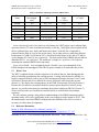
example_slitless.fits – This is the dispersed image through the F150W filter. Again,
it is best observed using a logarithmic scale. The X location of each target was chosen to place
all five orders (-1 to 3) on the chip. The zero- and first-order spectra are reproduced in Figure
3-1. The top four galaxies clearly show the emission feature in each redshifted spectrum.
3-5
Check with the JWST SOCCER Database at: https://soccer.stsci.edu
To verify that this is the current version.
NIRISS Wide-Field Spectroscopy Cookbook
JWST Mission Science & Operations Center
JWST-STScI-002949, SM-12
Revision -
Figure 3-1 Zero- and first-order spectra of the seven objects in our example.
The first object (bottom of figure) is a star with a flat spectrum, the second a galaxy generated with a 2-D
Gaussian, and the third a spiral galaxy using both a template image and a template spectrum. The last four
galaxies have identical spectra with a single emission feature, but with increasing redshifts that move the
emission feature across the bandpass.
Both the direct and dispersed images are normalized by the exposure time; that is, they have
units of e–/s. Both have the same toy file header with keywords appropriate for the
ACS/HRC/G800L, the default if aXeSIM does not recognize your instrument. We will modify
these keywords in Section 4.1.
example_slitless_2.SPC.fits – The SPC file contains the fully-calibrated, first-order
spectrum of each object in the field. It is a multi-extension FITS file; each spectrum is stored in
3-6
Check with the JWST SOCCER Database at: https://soccer.stsci.edu
To verify that this is the current version.
NIRISS Wide-Field Spectroscopy Cookbook
JWST Mission Science & Operations Center
JWST-STScI-002949, SM-12
Revision -
a separate FITS binary table extension with two columns, wavelength and flux density. The file
format is detailed in Section 4.9.1 of The WFC3 Cookbook. Note one cheat: aXeSIM performs
its spectral extraction on a version of the dispersed image with no sky background, so the
background subtraction is always perfect.
example_slitless_2.STP.fits – The STP file contains a two-dimensional image of
each first-order spectrum. It, too, is a multi-extension FITS file; each spectrum is stored in a
separate FITS image extension. The file format is detailed in Section 4.9.2 of The WFC3
Cookbook.
The SPC and STP files are standard output products of the aXe extraction routines. They were
generated by aXeSIM because we set the parameter extraction = yes. Because these
routines use the values of A_IMAGE, B_IMAGE, and THETA_IMAGE in the MOT, these
parameters should have reasonable values, even if a template image of the object is provided.
template_images.fits – This is an intermediate data product. Each image in the
template image list is normalized to an integrated intensity of 1.0 and stored in a separate FITS
image extension. Even if multiple entries in the MOT use a particular image, only one copy is
stored in this file.
template_spectra.fits – Another intermediate data product. Each spectrum in the
template image list is redshifted to the requested value, scaled to the requested magnitude, and
written to a separate FITS binary table extension. Because multiple entries in the MOT may use
the same spectrum with different redshifts or scalings, each entry in the MOT that uses a
template spectrum will generate a separate FITS binary extension.
Copies of template_images.fits and template_spectra.fits also appear in the
DATA directory.
A couple of files are modified by aXeSIM. In the DATA directory, half a dozen additional
columns are written to the MOT. These can be safely ignored, except for MODSPEC, which
lists, for each target that employs a template spectrum, the extension in the file
template_spectra.fits containing the redshifted and rescaled version of that spectrum. Note that
aXeSIM rounds the redshift values to a single decimal place, changing (0.0, 0.075, 0.15, 0.22) to
(0.0, 0.1, 0.1, 0.2).
In the CONF directory, a new copy of the configuration file has appeared with the suffix
.simul. It is merely a reformatted version of the original.
A note about redshifts: We have seen that aXeSIM rounds the redshift values to a single
decimal place in the modified version of the MOT. Figure 3-1 was generated using the script
run_example.py. If instead IRAF/PYRAF is run interactively and simdata called from the
command line (using the argument list in Section 3.3), aXeSIM will round the redshifts to a
single decimal place before generating the dispersed image. Of the four galaxies at the top of the
figure, the middle pair (objects 5 and 6) will have identical spectra with a redshift z = 0.1.
3.5
Reference Documents
Kümmel, M., Walsh, J. R., Kuntschner, H., & Bushouse, H. 2011, aXe User Manual, Version 2.3
Kuntschner, H., Kümmel, M., Walsh, J. R., & Lee, J. C. 2012, The WFC3 IR Grism Data
Reduction Cookbook, Version 1.15
3-7
Check with the JWST SOCCER Database at: https://soccer.stsci.edu
To verify that this is the current version.
NIRISS Wide-Field Spectroscopy Cookbook
JWST Mission Science & Operations Center
JWST-STScI-002949, SM-12
Revision -
Robberto, M. 2009, “A Library of Simulated Cosmic Ray Events Impacting JWST HgCdTe
Detectors,” JWST-STScI-001928
3-8
Check with the JWST SOCCER Database at: https://soccer.stsci.edu
To verify that this is the current version.
NIRISS Wide-Field Spectroscopy Cookbook
JWST Mission Science & Operations Center
4
JWST-STScI-002949, SM-12
Revision -
Prepare Input Files for Spectral Extraction
We move to the SAVE directory, where we will construct all of the input files required by aXe.
Some of the aXe routines modify their input files, so we will leave copies here for safekeeping.
4.1
Copy and Modify Image Files
Both the direct and dispersed images produced by aXeSIM have header keywords appropriate
for the ACS/HRC/G800L. We retrieve these images from the OUTSIM directory and modify
their file headers. Finally, we copy the FITS image extension containing the direct image into a
separate file.
>
>
>
>
>
>
cd SAVE
cp ../OUTSIM/example_direct.fits .
cp ../OUTSIM/example_slitless.fits .
modify_header.py example_direct.fits
modify_header.py example_slitless.fits
copy_extension.py example_direct.fits sci example_direct_sci.fits
All of the above steps have been combined into a single python script, which should be run from
within the SAVE directory.
> run_modify_files
4.2
Use SExtractor to Construct New MOT
When wide-field slitless spectroscopy is performed using HST, a direct image is always obtained
in the same visit as the dispersed image. A catalog derived from the direct image is used to
identify spectra for extraction with aXe. Assuming that JWST will be used in the same way, we
employ SExtractor to catalog the objects in our direct image.
SExtractor requires a pair of input files: a configuration file (example.sex) describing the data
and a parameter file (example.param) listing the object parameters that the program should
tabulate. The configuration file is described in Section 4.2 of the SExtractor User’s Manual,
while the list of parameters required by aXe is discussed in Section 7.2 of the aXe User Manual.
You can see which values in the configuration file we have changed by comparing our version
with the default:
> sex –d > default.sex
> diff default.sex example.sex
In particular, we have modified
DETECT_MINAREA
7
Default value is 5
DETECT_THRESH
3.0
Default value is 1.5
ANALYSIS_THRESH 3.0
MAG_ZEROPOINT
28.1844
Default value is 1.5
Yields 1 e-/s through F150W
GAIN
Exposure time; used in calculating magnitude errors
100.0
PIXEL_SCALE
0.064
SEEING_FWHM
0.08
CHECKIMAGE_TYPE APERTURES
Size of pixel in arcsec
Stellar FWHM in arcsec
4-1
Check with the JWST SOCCER Database at: https://soccer.stsci.edu
To verify that this is the current version.
NIRISS Wide-Field Spectroscopy Cookbook
JWST Mission Science & Operations Center
JWST-STScI-002949, SM-12
Revision -
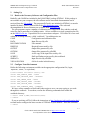
CHECKIMAGE_NAME apertures.fits
Figure 4-1 Detail of apertures.fits showing that SExtractor has identified our spiral galaxy as five separate
objects.
Setting the CHECKIMAGE keyword to APERTURES will cause SExtractor to generate a
copy of the input image with apertures drawn around the identified objects.
We have not changed FILTER_NAME, the kernel used to smooth the image before bright
regions of the image are separated into different objects. We use the default kernel, default.conv,
a pyramidal function with FWHM = 2. For this exercise, a more sophisticated kernel is
unnecessary, but you might try playing with others later on. If you are not using a machine at
STScI, you must edit FILTER_NAME, giving the full path to default.conv on your machine.
Now run SExtractor:
> sex -c example.sex example_direct_sci.fits
Output files are F150W.cat and apertures.fits. The catalog lists 11 (or more) objects, which is
odd, because we created only seven. A quick perusal of the image in apertures.fits (reproduced
in Figure 4-1) reveals that parts of our large spiral galaxy were identified as separate objects.
Rather than play with the detection parameters in the SExtractor configuration file, you can
simply delete the extra entries (those whose X coordinates differ from 900 by more than a couple
of pixels) from the catalog.
While you are modifying the catalog, please change the magnitude header keyword from
MAG_AUTO to MAG_F1498. One of the aXe routines will use the magnitude of each object to
4-2
Check with the JWST SOCCER Database at: https://soccer.stsci.edu
To verify that this is the current version.
NIRISS Wide-Field Spectroscopy Cookbook
JWST Mission Science & Operations Center
JWST-STScI-002949, SM-12
Revision -
compute its flux density, and it needs to know the wavelength at which the magnitude was
measured. Another aXe routine will use these magnitudes to estimate the contamination from
overlapping orders.
There may be other reasons to tinker with the output catalog. If SExtractor cannot estimate a
magnitude for an object, then it assigns a magnitude of 99. This value will lead to an error in the
aXe reduction software. Either replace the magnitude with a realistic number or remove the
object from the catalog.
4.3
Construct Input Image List
aXe requires an Input Image List that links together the various input files. The format is
[name of grism image] [object catalog] [name of direct image]
In our example, the file GR150R.lis contains the single line
example_slitless.fits F150W.cat example_direct.fits
4.4
Move Files into Position
We leave the files that we have just generated in the SAVE directory and place copies in the
directories where aXe expects to find them:
> cp GR150R.lis ..
> cp example_direct.fits example_slitless.fits F150W.cat ../DATA
or simply run this script:
> run_copy_files
4-3
Check with the JWST SOCCER Database at: https://soccer.stsci.edu
To verify that this is the current version.
NIRISS Wide-Field Spectroscopy Cookbook
JWST Mission Science & Operations Center
5
JWST-STScI-002949, SM-12
Revision -
Extract Spectra from Dispersed Image
Before running aXe itself, please return to the main cookbook directory.
5.1
Preparing the Spectral Extraction: axeprep
This program subtracts the background from the dispersed image. It also creates a file listing, for
each object in the catalog, the boundaries of each order and the flux therein. The fluxes will not
be computed if the catalog contains the header keyword MAG_AUTO, so double-check that you
have changed it to MAG_F1498. To run the program, enter
axeprep GR150R.lis NIRISS.F150W.conf backgr=’yes’
backims=’NIRISS.GR150R.sky.V0.fits’ norm=’no’
or use our handy Python script:
> run_axeprep.py
5.2
Extracting Individual Spectra: axecore
Finally, we run aXe itself, but with command-line arguments slightly different from those
employed by The WFC3 Cookbook:
axecore GR150R.lis NIRISS.F150W.conf extrfwhm=4.0 drzfwhm=3.0
back=’no’ backfwhm=0.0 orient=’yes’ slitless_geom=’yes’
cont_model=’gauss’ sampling=’drizzle’ lambda_mark=1500
We have changed the parameters orient and slitless_geom to “yes.” These commands tell aXe to
tilt the extraction window by the rotation angle THETA_IMAGE of the galaxy, thus improving
the resolution of the extracted spectrum.
Again, we provide a Python script to save you some typing:
> run_axecore.py
The output files generated by aXe are thoroughly documented in Section 4.9 of The WFC3
Cookbook, and we will not repeat that discussion here. In addition, we direct your attention to
the discussion of quality control in Section 5.1 of that document.
5.3
Reference Documents
Kuntschner, H., Kümmel, M., Walsh, J. R., & Lee, J. C. 2012, The WFC3 IR Grism Data
Reduction Cookbook, Version 1.15
5-1
Check with the JWST SOCCER Database at: https://soccer.stsci.edu
To verify that this is the current version.
NIRISS Wide-Field Spectroscopy Cookbook
JWST Mission Science & Operations Center
6
JWST-STScI-002949, SM-12
Revision -
Creating Web Pages to Review Your Results
The creators of aXe have provided a handy tool for displaying the program’s output products.
The program, aXe2web, constructs web pages showing the direct image, the two-dimensional
spectrum, and the extracted spectrum in units of both e–/s and erg/cm2/s/Å for each object in the
catalog. This tool is thoroughly documented in Section 5.2 of The WFC3 Cookbook, but we
supplement that discussion with information specific to our NIRISS simulation. In particular,
because we do not employ axedrizzle, we must use the output products of axecore directly.
• Step 1: Move to the visualization directory
> cd VISUALIZATION
•
>
>
>
>
Step 2: Copy all of the necessary files into place.
cp
cp
cp
cp
../SAVE/example_direct_sci.fits .
../DATA/F150W.cat .
../OUTPUT/example_slitless_2.SPC.fits .
../OUTPUT/example_slitless_2.STP.fits .
or just use our script
> get_vis_files
•
Step 3: Make a parameter file to control the program. Ours is GR150R.par:
#
# Example
#
pagename = GR150R
direct_image = example_direct_sci.fits
stamp_image = example_slitless_2.STP.fits
spectr_table = example_slitless_2.SPC.fits
sextract_cat = F150W.cat
sort_column = MAG_F1498
page_header = "aXe2web GR150R"
pagesize=50
error_bars=yes
mark_sources=yes
outputpath=web_pages
lambda_range=13000,17000
#
•
Step 4: Run aXe2web with the parameter file.
> aXe2web --parfile GR150R.par
If your computer replies, “Command not found,” then you must install aXe2web, which is
available from the aXe distribution page.
• Step 5: Review the output.
> open web_pages/GR150R.html
6-1
Check with the JWST SOCCER Database at: https://soccer.stsci.edu
To verify that this is the current version.
NIRISS Wide-Field Spectroscopy Cookbook
JWST Mission Science & Operations Center
JWST-STScI-002949, SM-12
Revision -
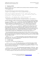
Figure 6-1 Output of aXe2web, showing the direct image, the two-dimensional spectrum, and the extracted
spectrum in both counts and flux units for each object in the catalog.
As shown in Figure 6-1, objects are sorted by magnitude and retain the object number from the
catalog. Our use of a tilted extraction window results in 2-D spectra in which the galaxies appear
to be aligned perpendicular to the spectral trace, resulting in much narrower emission features
than would otherwise be the case. If present, the blue line in the flux-calibrated spectral plots
represents aXe’s estimate of contamination due to background sources. It is zero for all of our
objects, so does not appear in these plots.
The count-rate spectra drop to zero at the edges of the filter bandpass, but the flux-calibrated
spectra rise sharply in the same regions. This discrepancy reflects a limitation in the sensitivity
curves, which are derived from observations of point sources (or in our case, from simulations of
point sources) but applied to extended objects. The effect can be reduced by setting the
parameter adj_sens=’yes’ in the call to axecore, which instructs aXe to smooth the
sensitivity function by convolving it with a Gaussian kernel scaled to the width of the object.
See the discussion of flux conversion in Section 1.11 of the aXe User Manual.
6-2
Check with the JWST SOCCER Database at: https://soccer.stsci.edu
To verify that this is the current version.
NIRISS Wide-Field Spectroscopy Cookbook
JWST Mission Science & Operations Center
6.1
JWST-STScI-002949, SM-12
Revision -
Reference Documents
Kümmel, M., Walsh, J. R., Kuntschner, H., & Bushouse, H. 2011, aXe User Manual, Version 2.3
Kuntschner, H., Kümmel, M., Walsh, J. R., & Lee, J. C. 2012, The WFC3 IR Grism Data
Reduction Cookbook, Version 1.15
6-3
Check with the JWST SOCCER Database at: https://soccer.stsci.edu
To verify that this is the current version.
NIRISS Wide-Field Spectroscopy Cookbook
JWST Mission Science & Operations Center
JWST-STScI-002949, SM-12
Revision -
7 Simulating Observations with GR150C
The configuration files used by the aXe programs describe the shape of the spectral trace, the
limits of each order, and the wavelength solution using functions of the horizontal axis X.
Because spectra dispersed vertically on the detector cannot be represented by such functions,
aXe cannot properly extract and calibrate them. To model vertically-dispersed spectra, we will
pretend that there is no grism GR150C and instead employ grism GR150R, combined with a
telescope rotation of 90°. To this end, we will rotate our model sky clockwise, which is
equivalent to rotating the telescope counter-clockwise.
7.1
Rotate the Catalog and Any Template Images
The following code fragment will rotate the input catalog by -90° (clockwise) about the center of
the detector:
x_rot = y_image
y_rot = 2041. - x_image
theta_rot = theta_image - 90.
if theta_rot < -90.:
theta_rot += 180.
This code is implemented in the Python script rotate_catalog.py. You can use it to rotate the
input catalog in the DATA directory. Since example.cat was modified by aXeSIM, use the copy
stored in example.save:
> cd DATA
> rotate_catalog.py example.save rotate.cat
Important: Suppose that your field is oriented with north on top. If you use horizontal
dispersion, then the spectra of the galaxies in the field are contaminated by the spectra of
galaxies that lie to the east and west of the field. If you use vertical dispersion, then the
contamination comes from galaxies to the north and south. If your input catalog is too small,
then your dispersed images will lack these overlapping spectra. Be sure that your input catalog
covers a sufficient area of the sky to provide these sources of contamination.
Because aXeSIM ignores the value of THETA_IMAGE when working with template images,
you must rotate each template image by hand. Here’s a little script to do that job:
> cd SIMDATA
> rotate_image.py spiral.fits spiral-90.fits
Be sure to modify the file cookbook/template_images.txt accordingly.
7.2
Rotate the Image Header
Now run aXeSIM as described in Section 3.3, but using the script run_rotate.py in place of
run_example.py. The resulting direct and dispersed images will appear as though the
telescope had been rotated by 90°. To complete the illusion, we must modify the World
Coordinate System keywords in the file header. To do this, simply add the argument “rotate” to
your call to modify_header.py, discussed in Section 4.1.
> modify_header.py rotate_direct.fits rotate
> modify_header.py rotate_slitless.fits rotate
7-1
Check with the JWST SOCCER Database at: https://soccer.stsci.edu
To verify that this is the current version.
NIRISS Wide-Field Spectroscopy Cookbook
JWST Mission Science & Operations Center
JWST-STScI-002949, SM-12
Revision -
Figure 7-1 Detail of rotate_slitless.fits showing the overlap of object spectra.
7.3
Further Analysis
You could proceed as before to extract and calibrate these spectra, but you may not want to. A
quick perusal of rotate_slitless.fits (reproduced in Figure 7-1) reveals that, because the
objects in our simulation are now aligned with the dispersion axis of the spectrograph, their
spectra (all five orders) overlap. Spectral overlaps occur on the real sky, of course, and aXe
provides tools for tracking and flagging them, but these tools are better explored using a less
toxic arrangement of sources.
It is possible to use drizzle routines to combine the horizontally- and vertically-dispersed
spectra. Instructions for doing so are provided in The WFC3 Cookbook. Keep in mind that, for
resolved objects like elliptical galaxies, the projection of the galaxy onto the dispersion axis –
and thus the spectral resolution – of the horizontally- and vertically-dispersed spectra may differ
significantly. You may find it better to model the two spectra separately, rather than combining
them.
7.4
Reference Documents
Kuntschner, H., Kümmel, M., Walsh, J. R., & Lee, J. C. 2012, The WFC3 IR Grism Data
Reduction Cookbook, Version 1.15
7-2
Check with the JWST SOCCER Database at: https://soccer.stsci.edu
To verify that this is the current version.