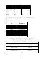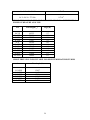
1
CORONAL DIAGNOSTIC SPECTROMETER
SOHO
CDS SOFTWARE NOTE No. 55
Version 5
August, 2003
SOHO CDS-GIS Analysis Guide
August 2003
Carl Foley
Solar and Stellar Physics Group,
Mullard Space Science Laboratory
University College London,
Holmbury St Mary, Dorking,
Surrey, RH5 6NT, UK
[email protected]
Revision list
Version 1, 19 May 1999
Original
Version 2, 1 July 1999
Converted to CDS software note 55
Version 3, 23 July 1999
Added approximate wavelength coverage;
added /cross_cor keyword to ghost_plot_one;
described ghost_info;
added /plot and /hardcopy keywords to ghost_buster;
ghost_buster prints wavelengths with the ghost cursor;
added section on saving and restoring ghost sessions;
gis_calib uses new calibration coefficients;
described gis_write_calib;
added the new routines to Appendix A.
Version 4, 11 Jan 2000
Expanded section on wavelength calibration
Version 5, August 2003
Added automatic option to ghost_buster and included associated ghost
information structures.
Added flat field files and correction to gis_calib.
Made photons/sec/arcsec2/cm2 default output from gis_calib, instead of
counts.
Included error tag to the calibrated qlds structure from gis_calib
Added new routine gis_fit which corrects, calibrates and fits the GIS data
non-interactively, providing the user with a simple entry into the analysis
of GIS data.
Included new gis_utplot plot routine.
Restructured and worded analysis guide throughout.
Put on web in HTML format with example programs etc.
2
Table of contents
1. Introduction ..............................................................................................................4
1.1 Related Documents......................................................................................5
1.2 GIS Observations........................................................................................5
2. Finding GIS Data.......................................................................................................6
2.1 Browsing the CDS Catalogue .....................................................................6
3. Reading and displaying GIS data..............................................................................7
4. Correcting GIS Data for Instrument Effects.............................................................8
4.1 Fixed Patterning ..........................................................................................9
4.2 Ghosts........................................................................................................10
4.2.1 Displaying GIS Ghost details.................................................................10
4.2.2 Finding Ghosts.......................................................................................10
4.2.3 Ghost Information files..........................................................................12
4.3 Ghost Correction.......................................................................................13
4.3.1 Ghost free mode.....................................................................................13
4.3.2 Manual mode .........................................................................................14
4.3.3 Saving and restoring ghost_buster sessions...........................................15
4.4 Edge effects...............................................................................................16
5. Calibrating GIS Data ..............................................................................................16
5.1 Wavelength Calibration.............................................................................17
5.2 Intensity Calibration..................................................................................17
5.2.1 Calibration details...................................................................................18
6. Using calibrated spectral data..................................................................................19
6.1 Extracting the data from the qlds ..............................................................19
6.2 Line fitting..................................................................................................20
6.3 GIS_FIT………………………………………………………………….21
6.4 GIS_UTPLOT……………………………………………………………21
Appendix A. List of useful routines.............................................................................23
Appendix B. Example Program....................................................................................24
Appendix C. Ghost free line lists ................................................................................25
3
1
Introduction
The objective of this document is to guide the user into the use of data obtained with the
Coronal Diagnostic Spectrometer’s Grazing Incidence detector, (GIS) which is part of the
SOHO payload. This document should be used in combination with the instrument guide
which contains more detailed information with regard to the detectors and their in-flight
characteristics. It is recommended that the instrument guide is read first, and then the analysis
process described here followed.
Reading and calibrating the GIS data is simplified greatly by using the Solarsoft IDL
library which is maintained and distributed at Lockheed Martin
(http://www.lmsal.com/solarsoft ). It is also available at the Solar UK research Facility at
MSSL ( http://surfwww.mssl.ucl.ac.uk/solarsoft ), where full instructions and support for
the installation and maintenance of the software is available. Some familiarity with the
IDL analysis package is assumed and Solarsoft is assumed.
To make the CDS libraries available on unix platforms and invoke IDL within SolarSoft use
the system commands:
setssw cds
sswidl
If using the CDS operations version of the IDL software (available from the Rutherford
Appleton Laboratory) then try the system command cidl, though this may vary at different
sites. Many routines are available within the CDS SolarSoft library (some useful ones are
summarized in Appendix A). To find which routines which are available for a particular task
use the IDL command (‘[ ]’s enclose optional inputs):
IDL> tftd,’search_string’ [, lines=lines, /prog, cat=cat]
This searches the CDS SolarSoft IDL directories for all occurrences of the search word in
routine descriptions. For more information about individual routines read the routine header
documentation with:
xdoc, ’routine_name’
or
doc_library,’routine_name’
In the following sections we describe the analysis techniques which may be used with the
GIS data. It is recommended that the ‘doc_library’ routine is used to investigate each of
these routines further since the headers contain a lot more information, and available
options which are omitted here for clarity.
4
1.1
Related Documents
The GIS software forms part of the CDS SolarSoft package put together at RAL, Oslo,
Goddard, MSSL, and other places.
The associated CDS Software notes are particularly useful and they come as part of the
CDS SolarSoft program library distribution. A few of them are listed below; all the notes
can be obtained from the web at
http://orpheus.nascom.nasa.gov/cds/software_notes.html.
CDS software note 54 - The GIS Instrument Guide, a detailed description of the
GIS instrument.
CDS software note 20 - CDS Quicklook Software User Manual is an introduction
to the general CDS software available.
CDS software note 22 - CDS on-line help utilities. To find your way about the
IDL software in the CDS SolarSoft distribution.
CDS software note 9 - The CDS Quicklook Data Structure. Gives more
information about the ‘quick look data structure’ (qlds) and the data within it.
CDS software note 47 - The Component Fitting System for IDL. For fitting
Gaussians/Voigt profiles etc. to spectra.
CDS software note 37 - Diagnostic Line Ratios (using CHIANTI) for CDS. Using
the CHIANTI atomic physics databases with CDS data.
CDS software note 33 - The CHIANTI Synthetic Spectrum Program for
CDS/SUMER.
CDS software note 50 - Differential Emission Measure analysis using CHIANTI.
5
1.2
GIS Observations
Unlike the NIS, observations with the GIS are astigmatic, and the whole of the
spectrometer slit is used to produce the spectra. To cover an area larger than the normal
GIS slits (2”_2”, 4”_4”, and for observations away from the solar disc 8”_50”) the scan
mirror and slit are moved over an area of up to 4 arc minutes. Data from all four detectors
are gathered simultaneously, and although the minimum integration time is 1 second per
pointing, it takes about 15 seconds to transmit the data. Thus to cover an area of 20”_20”,
using the 4”_4” slit and 50 second integration time per position takes just over 20
minutes. Because the GIS electronic encoding is sensitive to the incoming count rate,
different GIS set-up (GSET) parameters are needed for different expected count rates.
Much of this selection process is automated when the observation is uplinked to the
spacecraft, although the observer must specify the solar ‘zone’ beforehand. The zone is a
rough description of the solar activity expected in the observation. It can be one of:
•
•
•
off limb: not on the solar disk. The expected maximum detector count rates for
these areas are below 5 counts/second/pixel.
quiet sun: any quiet area of the sun, including coronal holes. The expected
maximum count rates are 20 counts/second/pixel.
active region: active regions, including those on the limb. The expected maximum
count rates are above 20 counts/second/pixel.
Once the zone and other observation parameters (raster size, slit, exposure time, exact
location, etc.) are determined, the CDS planner at the Experiment Operations Facility can
insert the GIS observation into the current plan. The combination of zone and slit selected
will prompt the CDS planner to choose an appropriate GSET. The GSETs themselves are
pre-determined from special (raw) observations made with the GIS. A number of raw
observations for each zone, each slit, each detector and for various high voltage settings,
are examined by the GIS team at MSSL and the best selected to produce the current set of
GSETs. The raw files associated with each GSET are also used to produce ghost
information structures and files. These enable likely ghosting regions to be identified, and
in many cases corrected for automatically, see section 4.3.
2 Finding GIS data
The CDS mission dataset can be browsed interactively using the powerful widget based
‘xcat’ routine.
IDL> xcat [, qlds, tstart=tstart, tend=tend]
A lot of progress can be made using this routine, such as displaying images and spectra. It is
a good idea to play with the menus at this stage if you haven’t already done so. For example
try selecting ‘GIS only’ from the ‘Detector’ menu, and put the required dates in the ‘Start
Time’ and ‘Stop Time’ fields, and try selecting each of the read file options.
6
It is also possible to investigate the databases directly using the ‘list_exper’ routine. This
route is particularly useful when you want to find data automatically within one of your own
IDL programs.
IDL> LIST_EXPER,’18:00 21-Jan-1998’,’21:00 21-Jan-1998’, OBS, N_FOUND
The output ‘obs’ is an IDL structure which contains full details of the observations which
CDS performed between the selected times. You can get an idea of the contents by typing:
IDL> help, obs, /str
You can use simple logic to select particular observations. For example to select all the GIS
observations performed in the selected time interval:
IDL> gis=where(OBS.detector eq 'G')
IDL> print, OBS.filename(gis)
3
Reading and displaying GIS data
The SOHO CDS data are stored and distributed in FITS format, which can be read into a
‘quick look data structure’ (qlds) using the ‘readcdsfits’ routine. For example, to read in the
GIS data set defined as study number s4384 raster r00:
IDL> qlds = readcdsfits(’s4384r00’)
The qlds contains the spectral data, some wavelength calibration information, ancillary
information about spacecraft pointing, and much more in a hierarchal structure similar to that
obtained using the LIST_EXPER routine (mentioned in the previous section). It is possible to
browse all the information in the qlds with the following
IDL> help, qlds, /str
This will display the following:
QL_ID
DOUBLE 1.0570199e+009 QL_NO
INT
HDRTEXT
STRING Array[481]
HEADER
STRUCT -> HDRX Array[1]
DETDESC
STRUCT -> GISXX3 Array[4]
BACKGROUND INT
0
WAVECAL
STRUCT -> GIS_WAVECAL Array[1]
DEL_TIMEDATA DOUBLE Array[20]
DEL_TIMEDESC STRUCT -> AUX2 Array[1]
INS_XDATA
FLOAT Array[20]
INS_XDESC
STRUCT -> AUX2 Array[1]
INS_YDATA
FLOAT Array[20]
INS_YDESC
STRUCT -> AUX2 Array[1]
…….
The structure can be investigated further in the following fashion.
IDL> help, qlds.header.gset_id
7
1
This will display the GSET for this observation. This embedding of information with the data
is a powerful method of distributing the data and greatly simplifies the analysis process,
making easy to quickly display and analyse the raw data. For example to plot all four GIS
data windows you can use the routine ‘cds_snapshot’:
IDL> cds_snapshot, qlds [/spectra, /log, window=window]
Figure 1: cds_snapshot of GIS data, using the /log switch. The salt and pepper noise which can
be seen over this data is due to fixed patterning (described in section 4.1). This plot displays
spectra since the G2AL study is a sit and stare study. For rasters, cds_snapshot will display an
image, unless the /spectra switch is used.
4. Correcting GIS Data for Instrument Effects
4.1 Fixed Patterning
Fixed patterning, is an effect caused by the interaction of the GIS digital electronics
with the analogue detector read-outs; it is very pronounced in some parts of the GIS
spectra. Figure 2 shows a subset of data from detector 1. A boxcar smooth of the
data will reduce the fixed patterning seen in the figure but increase the line widths
somewhat; the increase depending on the size of the boxcar used. Thus instead a
convolution with a Hanning function is used in the program gis_smooth. This
function preserves the total counts in the spectral lines, without introducing artifacts
in the background, or increasing the line widths.
8
Figure 2: A plot of the data around an Fe XI line from study 10716, showing fixed
patterning (left plot), where data shows large variations from pixel to pixel. The right plot
shows the same data after running gis_smooth.
To smooth the data within a qlds use:
IDL> gis_smooth, qlds [, smoothsize=size]
The option smoothsize exists to change the size of the function used, but the default
(smoothsize=7) works under normal circumstances. To assist with the smoothing
operation, any missing data in the data set are estimated automatically, the smooth
function is applied, and then the original missing data marked as missing again. It is not
recommended to replace missing GIS data separately before using any of the GIS
processing software; it is taken into account already by the programs.
9
4.2 Ghosts
An effect in the GIS detectors is the presence of ‘ghosts’. These are displaced spectral
lines, or parts thereof, caused by an ambiguity in the encoding used by the electronics.
The routine ghost_buster is used to remove or return ghosts in the GIS data.
When the GIS is in raw data mode, it transmits the data from one detector as a series of
coordinate pairs from the detectors. When these coordinates are plotted they form a spiral
(see the GIS Instrument Guide) where the spectral dimension lies along the length of the
spiral, and the intensity is the number of counts at each position along the spiral. To
translate these pairs into spectral position, a Look up Table (LUT) is used as part of the
on-board GIS processing. The parameters that define the LUT, plus the high voltage
setting, form the GSET mentioned earlier. Every GSET includes a different set of LUT
parameters, and the LUTs are calculated by the on-board GIS processor for each detector
immediately before the first observation using that GSET. The ambiguity (or ghosting) in
spectral data does not occur over the whole spectral range, but where the thin spiral arms
broaden and overlap each other. If a spectral line is ghosted, it is confined to occur only
at specific locations in adjacent spiral arms.
These characteristics are used in ghost_buster to restore the ghosts to their original
locations. The counts in a ghost must be added to the counts at the original location to
produce the correct line intensity. In ghosted areas, which cover 40% to 50% of the data,
it is easier to separate the original line from ghosts where there are no blends. Thus
ghosted areas in quiet sun observations are easier to correct than in an active region;
although the unghosted areas remain unaffected for all observation zones.
4.2.1 Displaying GIS Ghost details
The output from ghost_plot_one (e.g., Figure 3) displays the GIS data with an emphasis
on sorting ghosts from the original data:
ghost_plot_one, qlds, detector_no [,/sample, /nm, /angstroms,/logscale, /pixels, $
waverange=[min, max], /cross_cor]
This routine allows switches to modify how the data are plotted. For instance, waverange
can be used to zoom into a particular region of interest, by specifying a minimum and
maximum wavelength to be plotted; and sample plots a sample theoretical spectrum.
The routine first adds all the data from an observation into one spectrum per detector,
then plots the data with information to help find possible ghosts. Figure 3 was produced
using:
IDL> qlds = readcdsfits(’s10716r00’)
IDL> gis_smooth, qlds
IDL> ghost_plot_one, qlds, 1, /sample, /angstroms
10
Figure 3: output from ghost_plot_one, (top-top) theoretical quiet sun
spectrum, (top-middle) left shifted spectrum, (top-bottom) right shifted
spectrum. (Bottom) Spectrum to be de-ghosted, with likely ghosting
regions shaded.
The areas of the resulting plot are described from the top:
Theoretical quiet sun spectrum: This is the spectrum requested with the /sample
keyword. There are a number of warnings that come with the sample spectrum,
see xdoc, ’ghost_plot_sample’ for details. The spectrum is intended only as
an aid to ghost restoration; the intensities of lines are only approximate.
• left shifted spectrum and (correlation): The spectrum plotted is a copy of the
observed data, but shifted to the left by one spiral arm. Any ghost that occurs can
only be from an original line one arm to the left or to the right. As the ghosting
scale is not linear, the amount of shift varies across the detector.
• right shifted spectrum, a copy of the observed data shifted to the right, with the
optional correlation.
•
•
SPECTRUM: The lower part of the plot contains a summary of the data, where
all the exposures in the observation have been added together. The grey boxes
underlying the plot are information from ‘ghost information files’; which show
where the ghosts are expected. The vertical scale is in arbitrary units to show
11
most of the lines, but to enhance the weaker lines plot logarithmically with
logscale.
If the cross_cor keyword is used, the correlation between the original and shifted
spectra is displayed. If the absolute cross correlation coefficient is greater than 50% it
plots a thick bar. This is only a guide to where ghosts may be located, and is easily
confused by line blends. By default the correlation is not plotted. To summarise the data
from all four detectors in a similar way use
IDL> ghost_plot_all, qlds [ /angstroms, /nm]
4.2.2 Finding Ghosts
The output from ghost_plot_one (Figure 3) can be used to check whether a line is
ghosted, or itself is a ghost. Suppose we have seen a line, and want to check it; for
example there is a spectral line on the plot between 160 and 161Å (these ghosts are now
corrected automatically by default, since they are located in non blending regions – see
section 4.3). This line is in the ghosting region defined by the shaded region on the plot.
The first check is to look at the ‘theoretical quiet sun spectrum’; it shows that there are no
lines at this location. This may be a fault with the theory; however further checking
shows that the ‘left shifted spectrum’ also has a line at this point. This strongly suggests
that the line at about 160Å is a ghost and needs to be pushed to the right to correct the
line. The manual ghost correction software explains the process of moving the line in
more detail, as well as overlaying a ‘ghost cursor’ on the plot. This cursor shows exactly
where lines would come from if they are ghosts. Alternatively, if we are familiar with this
area on the solar spectrum we know there is a FeXIII line at 202Å (see Appendix C). To
see whether this line needs correcting, first notice that it is a clear area of the plot, i.e., not
in a ghosting area. Neither the left nor right shifted spectra show lines at this point, and
thus this line is free from ghosts.
4.2.3 Ghost Information files and structures
The ghost information files contain the pixel locations of ghosting regions which aren’t
corrected for automatically by ghost_buster. All GSETS have a ghost information file,
which is stored with the other GIS calibration files located in the $CDS_GIS_CAL_INT
directory. Also located in this directory are the ghost information structures, which are
used by ghost_buster to automatically restore ghosts.
12
4.3 Ghost Correction
There are now three modes for ghost correction: automatic, manual and ghost free. By
default ghost_buster works in automatic mode. This automatically corrects for most ghosts
where they are not coincident on other lines and are resolvable.
IDL> ghost_buster, qlds [,/plot ,/hardcopy ,/nm]
This corrects for about half of the ghosts (or 70% of the data, see Figure 4).
Figure 4: Ghost_buster automatic restoration of ghosts. (Left) uncorrected
averaged smoothed spectrum. (right) The same spectrum corrected using
ghost_buster in automatic mode. This works well for quiet sun observations,
restoring almost all lines.
To correct the remaining ghosts, where the ghost lands in the location of another line,
manual mode is required. This is described below. However, if from using
ghost_plot_one, the region of interest does not need correcting then use ghost free mode.
Once the ghosted areas have been removed with this mode, then the data can be further
calibrated without problems. If the region does need correcting, then run in manual
mode. Care must be taken with manually corrected data; it is possible to run
ghost_buster without making any changes, yet the software still allows further
calibration. Because the corrected count rates must be used for the count rate dependant
gain depression calibration (see below), it is important to replace the ghosts in any region
of interest before calibrating further. Only ghosts of the lines within the region of interest
need to be moved, all others can remain in place without affecting the calibration. If
spectral lines need to be fitted, it is recommended to correct for ghosts first, calibrate the
data, and then fit the lines. In either mode, it is possible to run ghost_buster again in the
same or a different mode, although if it is run on the same detector a warning will be
13
displayed. To reset all spectra to the uncorrected state it is necessary to re-read the qlds
from the data file.
4.3.1 Ghost free mode
This mode uses the ghost information files (section 4.2.3) to return only those areas of the
GIS spectra that show very little (less than about 5%) or no ghosting.
IDL> ghost_buster, qlds, /free [,/plot ,/hardcopy ,/nm]
About half of each spectrum is returned. Ghost free mode is available for all GSETs. Use
the plot or hardcopy switches to see the changes applied to the qlds. After using ghost free
mode, blocks of data from the known ghosting regions will be missing from the qlds. The
areas remaining can be used without needing ghost correction.
4.3.2 Manual mode
Manual mode allows the user to move ghosted lines within a single detector. To run in
manual mode supply two parameters, the qlds and a detector number.
IDL> ghost_buster, qlds, detector_no [,/hardcopy, /nm , /sample, /logscale, /plot,
/angstroms, save=save_struct]
Manual mode allows the user to specify which GIS spectral lines to relocate. The
program gives hints by using ghost_plot_one (Section 4.2.1) to show the spectrum with
overlying spectra shifted both to the left and to the right, a cross correlation with these
spectra, and an estimate of the amount of ghosting in each direction. It also uses a ‘ghost
cursor’ to show exactly where a spectral line would ghost. The main cursor is a solid
vertical line; either side of it is a dotted ghost cursor. The dotted lines are where any
selected data will be moved to (i.e., they correspond to the next or previous spiral arms).
The spacing between the dotted lines and the main cursor vary across the spectrum, as do
the shifted spectra. Below the dotted lines and main cursor are printed the corresponding
wavelengths for those points. To move a ghost that has been identified, position the
cursor to the left of the ghost and press and drag the left mouse button over the ghost. For
instance, to move the ghost previously identified at around 160Å (Section 4.2.2), press
the mouse button with the cursor just to the left of 160Å, keep it depressed and move to
about 162Å (see Figure 5).
14
Figure 5: Manual relocation of ghosts using ghost_buster in automatic mode.
(top) the region around the ghosted line located at 160_ has been selected, and
(bottom) relocated to its parent line at 175 _.
Let go of the mouse and enter r in the terminal window to move the line to the right.
Repeat this procedure until all the lines of interest have been corrected. When moving a
ghost, remember to include enough background for line fitting on either side of the line of
interest. It is possible to restore more ghosts by running the program again, on the same
detector or any other. Use the /plot or /hardcopy keywords to see the final result;
alternatively use gis_plot or ghost_plot_one when finished.
4.3.3 Saving and restoring ghost_buster sessions
By adding the save = save_struct keyword, it is possible to save the ghost corrections
made in manual mode into an IDL structure variable. It is then possible to restore these
corrections to uncorrected data with
ghost_buster, qlds, detno, restore = save_struct [,/plot, /hardcopy]
For example:
15
IDL> ghost_buster, qlds1, 1, save = save_struct
IDL> save, save_struct, filename=’qlds1_det1.save’
and then at a later time
IDL> restore, ’qlds1_det1.save’
IDL> ghost_buster, qlds2, 1, restore = save_struct
The first call to ghost_buster is in manual mode, and the software will prompt for
corrections to the data as outlined above. The corrections are stored in an IDL save file.
The second call uses the restored information to reapply the corrections to a second data
set. Note that both qlds1 and qlds2 must use the same GSET; and that the same
detector (number 1 in this case) must be used.
4.4 Edge effects
Most detectors show edge effects, both as spikes and a gradual increase in the
background. There are many causes for these effects, notably: a compression of the
wavelength scale, causing an increase in the background; end spoiling in the
microchannel plates, where the strong electric fields diverge at the ends of the detectors;
changes in the solar background, mainly from the HeII continuum; and some very bright
(solar) lines, seen especially in detector 2. Preliminary corrections for the non solar
sources are now included in gis_calib. These have relatively large errors associated with
them (which are passed into the output structure). These will reduce as we acquire more
observations to check the corrections.
5. Calibrating GIS Data
The GIS calibration has recently been updated using the results of workshops which were
held at the International Space Science Institute (ISSI) during 2001. These
workshops were used to determine (using intercalibration observations) to find an
absolute and relative intensity calibration for all the instruments on SOHO. This resulted
in an overall upward shift in the sensitivity of the GIS by 2.6.
More recently it has been found that the lines in GIS 1 and 2 were becoming degraded
due to the effects of Long term gain depression. For this reason new flat field files have
been generated to correct for this degradation. Because of the size of the corrections (as
much as 60%) and associated uncertainty, a pixel by pixel error array is now included in
the calibrated qlds structure. This can be extracted using the gis_error function
IDL> error=gis_error(qlds,detno)
16
5.1 Wavelength Calibration
Wavelength calibrations are read in automatically when the fits file is converted to a qlds.
The wavelength calibration can be accessed by the routines wave2pix, pix2wave, which
translate the GIS pixel co-ordinates as necessary.
pixel = wave2pix(spec_id, wavelength [,/limit])
Where, for the GIS, spec_id is a string containing GIS1 GIS2 GIS3 or wavelength
can be a single value or an array. See the example program B. Similarly
wavelength=pix2wave(spec_id, pixel)
Which will return the wavelengths of the pixel array for the spectrum. Again, the input
can be a single value or an array. Variations of about 20% of a line width are expected
between observations, caused mainly by GIS hardware temperature differences when
observing different areas of the sun, or very high count-rates (more than about 40
counts/second/pixel) causing distortions in the electronic processing. Note that the
wavelength calibration varies with each GIS setup (GSET) compare two GIS
observations that used different GSETs it is necessary wavelength calibration. This is
simplified with the routine restore_wavecal. For instance, below is part of an IDL session
to over plot two GIS observations:
IDL> qlds_1 = readcdsfits('s8965r00')
IDL> qlds_2 = readcdsfits('s8966r00')
IDL> gis_smooth, qlds_1
IDL> gis_smooth, qlds_2
IDL> print,restore_wavecal(qlds_1) ; prints “1” If restored
IDL> wave_1 = pix2wave('GIS1', findgen(2048))
IDL> data_1 = gt_windata(qlds_1, 0) ; window 0 is for detector 1
IDL> print,restore_wavecal(qlds_2)
IDL> wave_2 = pix2wave(’GIS1’, findgen(2048))
IDL> data_2 = gt_windata(qlds_2, 0) ; window 0 is for detector 1
IDL> plot, wave_1, data_1/max(data_1), xrange=[187,190], psym=10
IDL> oplot, wave_2, data_2/max(data_2)
5.2 Intensity Calibration
As well as the ghosts and fixed patterning, the detectors and their electronics have nonlinearities that need to be corrected. On the whole these corrections are small (less than
10%, but dependent on count-rate). gis_calib will correct for these (as well as correct for
gain depression); and calibrate from counts into photons using the updated GIS
calibration coefficients.
gis_calib, qlds [,errmsg=errmsg, /quiet, /steradian_m2, /counts]
17
By default the data will be returned in calibrated units of photons/sec/arcsec2/cm2.To
convert to photons per second per solid angle per area use the /steradian_m2 or (to leave in
counts) /counts switches. The routine checks to make sure the routine ghost_buster has
been run for all the detectors - if not the error for data in the regions likely to ghost is set
to 100% of the counts in the adjacent arms. Similarly, the error for regions which cannot
be calibrated for any other reason is also set; this might include the occasional strong line
that is too bright for the gain depression calibration (such as the HeII 304Å line), or
whole detector count rates too high for the electronic dead time corrections.
The GIS calibration coefficients used are those from the results of the SOHO radiometric
inter-calibration workshops which were held at the International Space Science
Institute (ISSI) during 2001. The coefficients can be viewed using the program
gis_write_calib.
5.2.1 Calibration details
The corrections and calibrations made by gis_calib include:
• FIFO dead time: The dead time is a straightforward correction for an on-board
First in First out (FIFO) event queuing chip. It applies to all four detectors
simultaneously, and involves a constant non extending dead time allowing 105
counts per second through unhindered, with small corrections for higher rates.
• Simple correction for Quiz-show dead time: The programmed Quiz-show
correction is simply an upper limit on the rates; if photon events are less than 6
microseconds apart then the data are marked as uncalibratable. The maximum
rate is then 1.0/(6.0_10-6) or approximately 1.7_105 over all four detectors.
• Analogue dead time: This involves an extending dead time of approximately 2_
microseconds. The data used to correct for this were measured before launch
using the flight electronics and are read from a data file.
• Count rate dependant gain depression (also known as short term gain
depression). If more than 5% error would occur in the measured rates, then the
datum (at that point only) is marked as uncalibratable.
• Long term gain depression and flat field: The correction is based on the total
accumulated charge extracted from the MCP’s.
• Detector / grating / telescope effective area. The calculations are based on a
ground based calibration exercise for the whole of CDS. The relative calibration
coefficients have since been verified in flight2, but please note that there is
currently a very large uncertainty in the absolute values.
18
6. Using calibrated spectral data
Various CDS and other SolarSoft routines exist to use the data once calibrated; most of
these can be used with both NIS and GIS data. The generic dsp_menu program will work
with both calibrated and un-calibrated data,
dsp_menu, qlds [, qlds2, qlds3, ..., /delete, /nocheck]
6.1 Extracting the data from the qlds
To extract the spectral data from a qlds always use gt_windata or gt_spectrum
data = gt_windata(qlds, window [,/nocheck, /quick, /nocopy, $
/nopadding ,errmsg=errmsg])
These routines will work with all storage schemes used for CDS qlds data. With GIS
data, specify the qlds and the ‘window’, which is one less than the detector number.
For example, to extract detector 3 data from a pre-defined qlds use
IDL> GIS3data = gt_windata(qlds, 2)
The returned data are a floating point array of up to 4 dimensions: spectrum (always 2048
pixels for the GIS), solar x, solar y, and time. The time dimension is only used for data
that have multiple exposures at the same solar x, y point. To get information about the
extracted data use
gt_windesc(qlds, window [,/nocheck, /quick, /errmsg]
For example:
IDL> GIS3desc = gt_windesc(qlds, 2)
The returned structure tells us which units the data use (GIS3desc.units), the missing
data flag (GIS3desc.missing), the wavelength range (GIS3desc.wavemin,
GIS3desc.wavemax), etc. The command
IDL> xshow_struct, GIS3desc
will display all the information available in the structure. Also available is
gt_spectrum, to get individual spectra from a raster:
result = gt_spectrum(qlds, window=window, yix=yix, xix=xix, $
[tix=tix, lambda=lambda, xsolar=xsolar, ysolar=ysolar, time=time]
Where window, yix, xix, tix are the user supplied window (i.e., the detector
number-1), and for each raster position the x, y and time indices. The time index is not
normally used unless the raster has repeated exposures at the same position. If supplied,
lambda will return the wavelength for each pixel in the spectrum, xsolar and ysolar
19
are the locations on the sun in arc seconds from the sun centre and time is the time of the
start of the exposure.
6.2 Line fitting
Many fitting procedures are available (see tftd, ‘gauss’ and tftd, ‘voigt’)
which can be used to fit various profiles and backgrounds to ghost free or ghost
corrected GIS spectra. One of these is ezfit:
ezfit, wavescale, data, waverange, k=k
where wavescale and data are the X and Y variables, waverange can be used to
limit the fit to a particular line, and k is the polynomial order of the background. Thus
to fit a Gaussian plus background to a region in the first exposure of the above GIS
detector 3 data:
IDL> wavescale = pix2wave('GIS3', indgen(2048))
IDL> data = GIS3data[*, 0, 0, 0]
IDL> waverange = [415, 420]
IDL> ezfit, wavescale, data, waverange, k=1
Another routine, cds_gauss, has been developed for use with CDS data:
yfit = cds_gauss(x, y, [a, k])
Where x is the independent vector; y is dependent variable; a contains the returned
coefficients and k defines the order of the polynomial to be fitted to the background.
A more complicated but very comprehensive fitting routine is cfit
yfit = cfit(x, y, a, fit [,sigmaa] [+keywords])
Where x, y are the data to be fitted, a is an array of (nominal) parameter values – if
defined then used as an initial guess to the fit; fit is a structure containing one tag for
each component in the fit; sigma contains the errors for each of the parameter values
in a. For detailed information about cfit see CDS software note 47 – The Component
Fitting System for IDL.
20
6.3
GIS_FIT
GIS_FIT uses predefined cfit structures to automatically fit most regions of the GIS spectra.
IDL> gisfit=gis_fit(qlds, [/plot],gisfit=gisfit)
This routine works on calibrated and uncalibrated data. Un-calibrated data is corrected and
calibrated automatically using the individual routines described in the previous sections of
the analysis guide (Gis_smooth, Ghost_buster, gis_calib etc). The visible identified lines
are then fitted, using the cfit line fitting routine. The output structure contains the fitted line
positions, widths, intensities, errors, and total line counts in photons/sec/arcsec2, along with
ancillary data such as the location and time of observation. The gisfit structure can be used to
quickly produce light curves, images and DEM maps
6.4
GIS_UTPLOT
To display a quick time series of data acquired with GIS you can use the routine
gis_utplot. This is a wrapper to the Solarsoft utplot program, which displays a time series
of the data acquired. To call:
IDL> gis_utplot, qlds, det_no [,uttime=uttime,gisfit=gisfit ]
This plots a time series of the raw accumulated counts for the selected detector (see
Figure 6).
Figure 6: The output from gis_utplot, for a series of sit and stare
observations in an active region located at the limb. Note the dimming
periods around 17:00 and 20:00 UT. This is investigated in Figure 7 where
individual lines are plotted.
21
This routine also works with arrays of qlds structures. So if you have a series of qlds from
a particular observation you can combine these in the following way:
IDL> gis_utplot,[qlds, qlds1, qlds2, qlds3], det_no [, lines=lines, gisfit=gisfit]
Or alternatively a string array of program numbers for example:
IDL> gis_utplot,[‘26320’,’26322’,’26324’], 1 [, lines=lines, gisfit=gisfit]
This will read, correct, calibrate and then plot the data, In this case from a sit and stare
observation which is displayed in Figure 6. The calibrated and fitted data is saved into
the gisfit structure if this variable is passed on the command line. If it already exists it is
updated. The gisfit structure can then be used to plot the corrected, calibrated and fitted
lines from the observations.
IDL> gis_utplot, gisfit
Calling gis_utplot in this fashion will result in a prompt for you to select a particular line
from a list of available present in the structure to plot. Alternatively, the specific line id
can be entered.
Figure 7: Output from gis_utplot, for specific lines contained in the gisfit
structure.
GIS specific software for determining, temperatures, emission measures, densities, and
DEM’s, based on the output gisfit structure, are under development. To find the latest
routines, browse using
IDL> doc_library,’gis*’
22
Appendix A. List of useful routines
Some useful CDS and other SolarSoft routines, along with one-line descriptions. For
detailed information examine the routine headers with xdoc, ’routine_name’.
cds_fill_missing
cds_gauss
cds_snapshot
chianti_ne
chianti_ss
chianti_te
cfit
dsp_menu
Ezfit
Ghost_buster
Ghost_info
Ghost_plot_all
Ghost_plot_sample
Ghost_plot_one
gis_calib
gis_plot
gis_smooth
gis_write_calib
gt_bimage
gt_spectrum
gt_windata
gt_windesc
integral_calc
mk_cds_map
pix2wave
plot_map
readcdsfits
show_struct
tftd
utplot
wave2pix
xcat
xcds_snapshot
xdoc
Fills MISSING pixels in QLDS.
Fits Gaussian with constant, linear or quadratic background
Makes a thumbnail sketch of images from a CDS study
Calculate and plot CHIANTI density sensitive line ratios
Calculates and plots CHIANTI synthetic spectrum
Calculate and plot CHIANTI temperature sensitive line ratios
Make a best fit of the sum of components to the supplied data
Selection of display modes for CDS QL data
Easy Gauss fit to data
Move GIS detector ghosts.*
Display the ghosting information associated with a QLDS*
Plots all 4 GIS detector data with likely ghost regions*
Plots (or returns) a theoretical sample GIS spectrum*
Plots a GIS detector data with likely ghost regions*
Applies calibration factors to GIS spectra.*
Summarise data from one GIS detector*
Smoothes GIS spectra to ’remove’ fixed patterning*
Prints calibration factors for GIS spectra*
Return wavelength band integrated image.
Returns one-dimensional spectrum at specified point
Return block of detector data from one detector window.
Return descriptor structure for one detector window
To compute the atomic data integral for use in column or volume
emission measure work.
Make an image map from a CDS QL structure
Calculate CDS wavelength given a detector pixel location.
Plot an image map
Read and return the contents of a CDS FITS level-1 file.
Display contents and breakdown of an IDL structure
Search for a string in header documentation
Plot X vs. Y with Universal time labels on bottom X axis.
Calculate detector pixel location given a CDS wavelength.
widget interface to CDS AS-RUN catalogue
Widget interface to CDS_SNAPSHOT
Front end to online documentation software.
23
Appendix B. Example Program
Below is an example program that combines a series of exposures, and plots the total
spectrum. The count rates within a section of the spectra are then plotted as an image.
pro example, study, detno, lam1, lam2
;
; study: study filename (string)
; detno: detector number, from 1 to 4
; lam1, lam2: wavelength range to integrate over (in Angstroms)
;
; e.g. to pick the 277A line in detector 2 in study s7060r00 type:
; IDL> example, ’s10716r00’, 2, 276, 278
;
; [email protected], 17 Feb 1999
;
print, ’Reading ’ + study, + ’, detector number’, + detno
print, ’Plotting between wavelengths ’, lam1, lam2
;
qlds = readcdsfits (study) ; read in the qlds
ghost_buster, qlds ; ghost free areas
gis_calib, qlds, /arcsec2_cm2 ; calibrate
cds_fill_missing, qlds ; guess missing data
;
; plot an average spectrum
;
window, 0
ghost_plot_one, qlds, detno, /angstroms
;
; Take a slice of the data
;
int_spec = gt_bimage(qlds, lam1, lam2, xsolar=xsolar, $
ysolar=ysolar)
;
spec_id = ’GIS’ + trim(detno)
print, ’Pixels chosen:’, wave2pix(spec_id, [lam1, lam2])
print, ’Bottom left position on the sun:’, $
min(xsolar), min(ysolar)
;
; plot the image
;
window, 1
loadct, 0
tvscl, congrid(int_spec, 512, 512)
;
return
end
24
Appendix C. Ghost free line lists
Below are tables of expected count rates per second for lines, for slit 1 (2”x2”), in
ghost-free areas in the four GIS detectors. The lists are originally from the CDS Scientific
Report (‘Blue Book’) by Richard Harrison, Tables 2.1-2.6 and 3.3-3.7 with lines in
ghosted areas removed. Note that this list is specifically for the ghost free areas of
observations taken with GSET 41 (quiet Sun, 2"_2" slit), although the positions of
ghosting are similar for all the GSETs. A detailed check of ghosting in an observation can
be made with ’ghost_plot_one, qlds, detno’
DETECTOR 1
Ion
Wavelength (Å)
Quiet Sun Intensity
Ni XIV
Ar X
Fe VIII
Ni XIV
Fe IX
OV
O VI
O VI
Fe X
Fe XI
Fe VIII/Ni XVI
Fe VIII
Fe XII
Fe VIII
Fe XI
S XI
Fe X
Fe XIII/SXI
Fe XIII
Fe XII/XIII
Fe XIII
S VIII
Fe XIII
Fe XIII
Fe XIII
SX
Fe XIII
Fe XIII
164.13
165.49
167 - 168
169.68
171.07
172.17
172.93 - 173.08
183.94 - 184.11
184.54
184.79
185.22
186.60
186.88
187.23
188.22
188.67
190.04
191.26
200.02
201.12
202.04
202.61
203.79
204.26
204.94
208.32
208.68
209.62
0.4
0.0
2.0
0.0
8.8
0.1
0.7
0.4
2.2
0.2
0.8
0.5
2.4
0.0
8.2
0.3
1.3
0.3
0.7
2.0
0.9
0.4
3.7
0.0
0.6
0.0
0.0
0.0
25
Si VIII / Si XII
Si VIII
Fe XII
S XII
Fe XIV
Fe XIV
214.76 - 215.15
216.90
217.27
218.18
219.12
220.08
0.8
0.6
0.0
0.4
2.0
2.6
DETECTOR 2
Ion
Wavelength (Å)
Quiet Sun
Intensity
Active Sun
Intensity
Si X
261.06
1.5
Fe XVI
262.98
1.3
Fe XIV
274.20
5.7
Si VII
275.37 - 275.76
0.5
Mg VII
276.15
0.2
Si VII / Si VII
276.77 - 276.85
0.2
Mg VII / Si X
277.04 - 277.27
2.3
Mg VII / Si VII
278.40
0.5
S XI
281.42
0.5
S XI
281.83
0.0
S XII
299.50
0.2
Fe XI
308.54
0.0
0.0
Fe XIII
318.14
0.9
2.9
Si VIII
319.83
1.3
2.5
Fe XIII
320.80
3.5
11.5
Fe XV
321.78
2.3
7.9
Fe XV
327.02
2.4
8.0
Fe XII
338.26
1.2
4.2
Note that the He II and blended Si XI lines at 304Å are not included because the
intensity of these excessively bright lines cannot be calibrated.
DETECTOR 3
Ion
Wavelength (Å)
Quiet Sun
Intensity
Active Sun
Intensity
Ne V
Fe XV
S XIV
C IV / Ca X
416.20
417.26
417.60
419.50 - 419.74
0.2
1.1
3.9
0.7
0.8
34.6
32.4
3.0
26
Mg IX
Mg IX
Ca XV
S XIV
Si IX * / Mg VII
Ne VII
Ca IX
Ne IV
Ne III
438.60
444.03
445.00
445.70
450.73
465.22
466.23
469.80
489.50
0.2
0.4
0.0
0.2
0.0
4.4
0.0
0.3
0.2
0.8
2.8
3.6
3.0
0.0
36.1
2.7
1.2
1.2
* Second order line blend
DETECTOR 4
Ion
Wavelength (Å)
Quiet Sun
Intensity
Active Sun
Intensity
N III
C II
Ca IX
Al III
Mg IX * / Ne I
OV
OV
OV
OV
N III
Ne VIII
S XI
Mg VIII
685.83
687.20
693.80
696.00
735.90
758.60
759.44
760.40
762.00
764.00
780.30
782.00
783.00
1.1
0.3
0.3
0.0
0.4
0.4
0.0
0.9
0.0
0.0
1.4
0.0
0.2
2.2
0.5
1.6
0.1
2.6
2.1
0.0
4.4
0.0
0.0
16.1
0.2
0.7
* Second order line blend
BRIGHTEST GHOST FREE LINES VISIBLE WITH THE GIS
The Si XI 303Å and He II 304Å line are not included because the intensity of these
excessively bright lines cannot be calibrated.
Ion
Wavelength (Å)
Fe IX
171.07
Quiet Sun
Intensity(counts/second)
8.8
27
Fe XI
Fe XIII
Fe XIV
Fe XIV
Fe XIV / Si VII
Fe XV / Al IX
Fe XIII
S XIV
Ne VII
188.22
203.79
220.08
264.79
274.20
284.16
320.80
417.60
465.22
8.2
3.7
2.6
4.2
5.7
22.3
3.5
3.9
4.4
GIS PRIME DENSITY SENSITIVE PAIRS IN GHOST-FREE REGIONS
Note the lines marked with 'n' are NIS lines
Ion
Wavelengths (Å)
Mg VII
S XI
S XI
S XI
Fe XII
Fe XIII
Fe XIII
Fe XIII
Fe XIII
Fe XIII
Fe XIII
280.74 / 278.40
215.93 / 281.42
190.37 / 281.42
217.64 / 281.42
338.27 / 364.47n
202.04 / 200.02
201.12 / 200.02
202.04 / 203.79
318.12 / 320.80
320.80 / 348.18n
318.12 / 348.18n
GIS GHOST-FREE TEMPERATURE SENSITIVE LINE RATIOS
Note that ’n’ is for NIS lines and ’s’ for SUMER lines
Ion and Ratio
Range of Sensitivity (K)
O V 172.17 / 629.73n
< 1.0 x 10⁶
O VI 173 / 1032s
< few x 106
O VI 184 / 1032s
< few x 106
28
105-106
Ne V 416.20 / 569.20n
105-106
Ne V 416.20 / 572.20n
GHOST-FREE LINES IN THE GIS RANGE SUITABLE FOR A DIFFERENTIAL
EMISSION MEASURE ANALYSIS
Ion
Wavelength (_)
LogT(K)
Ne VII
Ne VIII
Si VII
Si VIII
Si X
Fe VIII
Fe IX
Fe XI
Fe XIII
Fe XIV
Fe XVII
465.22
780.30
275.37
319.83
261.06
168.18
171.07
188.22
203.79
220.08
200.80
5.7
5.8
5.8
5.9
6.0
5.6
6.0
6.1
6.2
6.3
6.5
GHOST-FREE GIS LINES SUITABLE FOR HIGH TEMPERATURE STUDIES
Ion
Wavelength (Å)
Fe XXIII
Fe XXIII
Fe XXIII
Fe XXIV
Fe XXIII
Fe XXII
154.27
166.74
173.31
192.02
263.76
217.30
29