Download User`s Manual

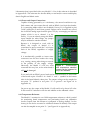
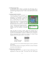
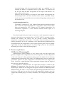
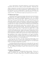
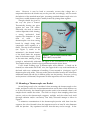
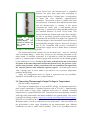
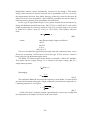
Glitch Laboratories
Thermocouple Sensor Board
Model 1.3
User Manual
Glitch Laboratories
“If it works, it’s a Glitch!”
v1.31 9/17/2004
i
Note: Glitch Laboratories is a fictiteous company.
It has no web site,
buildings, or other physical presence (though there are some mass spectrometers
at NASA that are/were using Glitch Laboratories controllers). It merely exists for
those moments when I get to putter at the electronics bench in my apartment.
Consequently, it cannot extend any kind of formal warrantee. But, I will do my
best to offer one:
Product warranty
I warrant that the Model 1.3 unit is free of defects and that it will operate at a satisfactory level of
performance for a period of one year from the original date of purchase. If the unit fails to operate as
specified, notify me within the warranty period. Modifications to the unit void the warranty.
On the other hand, I have tried really hard to produce something robust, useful,
(and worthy of the Glitch name… er, well, anyway). So, if you have a problem
with a Model 1.3 sensor board, please let me know. I will do all I can within
reason to make it better, especially if I like you and you seem to be intent on
having fun. (This is a hobby, after all.) However, here is some more legalese:
Product disclaimer and limit of liability
The Model 1.3 unit is intended for use in model, high power rockets only. Do not use this device for any
other purpose than specified in this manual.
Because the use and application of the Model 1.3 unit is beyond my control, the purchaser or user agrees to
hold me, Robert Brigham, harmless from any and all claims, demands, actions, debts, liabilities, judgments,
costs, and attorney fees arising out of, claimed on account of, or in any manner predicated upon loss or
damage to property of, or injuries to or the death of any and all persons arising out of the use of this
equipment. Due to the nature of electronic devices, the application and environments for those devices, the
possibility of failure can never be totally ruled out.
Life support applications
This product is not designed for use in life support appliances, devices, or systems where malfunction of
this product can reasonable be expected to result in personal injury. My customers using or selling this
product for use in such applications do so at their own risk and agree to fully indemnify me for any
damages resulting from such improper use or sale.
If you need to contact me, your best bet is by e-mail. I have been slogging along
with the same Compuserve account ( [email protected] ) for over 12 years and
don’t feel like changing just yet.
Robert Brigham
26500 Agoura Road PMB 336
Calabasas CA 91302
June 2004
NAR 79579 L2
ii
Table of Contents
1. INTRODUCTION................................................................................. - 1 2. MODEL 1.3 THERMOCOUPLE SENSOR BOARD................................. - 2 2.1 Overview................................................................................................................................................... - 2 2.2.1 Power and Output Connections ...................................................................................................... - 4 2.2.2 Temperature Reference...................................................................................................................... - 4 2.2.3 Thermocouple Status.......................................................................................................................... - 5 2.2.4 Thermocouple Connections.............................................................................................................. - 5 2.2.5 Placement of the Model 1.3............................................................................................................... - 5 2.2.6 Mounting the Model 1.3 .................................................................................................................... - 6 -
3. THERMOCOUPLE BASICS................................................................... - 6 3.1 What is a Thermocouple? ..................................................................................................................... - 6 3.2 Thermocouple Types ............................................................................................................................. - 7 3.2 Making a Thermocouple ...................................................................................................................... - 7 3.3 Mounting a Thermocouple on a Rocket ........................................................................................... - 8 3.4 Converting Thermocouple Output Voltage to Temperature...................................................... - 9 3.5 Examples of Rocket-borne Temperature Profiles ........................................................................ - 11 -
APPENDIX A: CALIBRATION PROCEDURE......................................... - 13 APPENDIX B: DISPLAYDATA SOFTWARE........................................... - 15 B1. DISPLAYDATA PROGRAM............................................................. - 15 B1.1 Loading the DisplayData Program................................................................................................ - 15 B1.2 Loading Data....................................................................................................................................... - 16 B1.3 Select Thermocouple Type.............................................................................................................. - 16 -
iii
B1.4 Enter Calibration Values ................................................................................................................. - 17 B1.5 Select Data to be Displayed ............................................................................................................ - 17 B1.6 Produce Data Plot .............................................................................................................................. - 18 B1.7 Enlarge Plot Area ............................................................................................................................... - 18 B1.8 Enable Cursor ..................................................................................................................................... - 19 B1.9 Plot Units.............................................................................................................................................. - 20 B1.10 Plot Title ............................................................................................................................................. - 20 B1.11 Plot Colors ......................................................................................................................................... - 20 B1.12 Smoothing Data ............................................................................................................................... - 20 B1.13 Saving Plots....................................................................................................................................... - 21 B1.14 Saving Data ....................................................................................................................................... - 21 B1.15 Saving Settings ................................................................................................................................. - 21 B1.16 Exit ....................................................................................................................................................... - 21 -
APPENDIX C: MOUNTING TEMPLATES .............................................. - 22 -
iv
1. Introduction
The Glitch Laboratories Model 1.3 temperature sensor board is designed to be used in
high power rockets as a means of gathering temperature data. It has a very fast
response time, on the order of a tenth of a second, is small, and light. Without offset, the
board produces a voltage resembling temperature in °F for both type T and K
thermocouples (i.e., 45°F produces a nominal signal level of 0.45 volts). The board
operates from a single-sided power supply, so it cannot pr oduce a negative voltage for a
negative temperature. This is circumvented by adding 1 volt to the output offset (so in
the example above 45°F actually produces a nominal value of 1.45 volts.). Allowing for
the non-linearities of thermocouple response, this allows measurement of temperatures
below -100°F (-73°C).
The Model 1.3 is a product, first, of my desire to put a high power rocket to good use,
and second, my curiosity about the weather and atmosphere borne of my experience as
a pilot.
My high power rocketry activities have been carried out at Lucerne Dry Lake in Lucerne
Figure 1. Lucerne Dry Lake, Lucerne Valley, CA. It’s big and it’s flat.
Valley, California. This location (Figure 1) at the edge of the Mojave Desert, lies at an
elevation of 2900’ (880m) is surrounded on three sides by mountains of varying heights
(note background in Figure 2), the highest being the San Bernardino Mountains to the
south which reach over 8000’ (2400m). Except during occasional winter storms, weather
at this location is marked by calm conditions that extend from the early morning hours
to early afternoon, at which time cooler air flowing from the coast through Cajon Pass
moves in to displace warmer desert air. In the winter the temperature difference is small
and little or no afternoon breeze arises. In the summer months, the afternoon zephyr
can be ferocious.
-1-
Meteorologists and pilots will tell you that
an enclosed basin under still, clear, starry
skies, will fill up with cold stable air as the
night progresses. This gives rise to a
temperature inversion, i.e., temperature
goes up with altitude, not down. Noticing
the slow and often complex drift of rocket
exhaust plumes in the almost dead calm air
of many Lucerne Valley mornings, I
became curious about the air that was
moving them.
Thus was born the idea of flying a
sensor that could measure and record air
temperature during flight. (Have you
figured out by now I’m a geek.) The sensor
had to be light, simple, stable, and fast.
The
average
semiconductor
temperature sensor, while possessing most
Figure 2. Gratuitous photo of my
of these qualities, is quite slow. Response
Ultimate Endeavor flying on an
time of these devices is drastically reduced
Aerotech K700 at Lucerne Dry
by the thermal inertia of the encapsulation
Lake, Dec/2002.
material and housing. For example, a LM34
in a plastic TO-92 housing make take in excess of 8 minutes to thermally equilibrate
with its surroundings. A typical high power rocket flight, from ascent to touchdown,
is usually over in half this time. The best type of temperature sensor that is simple,
rugged, and fast enough to work in a rocket borne probe is a thermocouple.
2. Model 1.3 Thermocouple Sensor Board
2.1 Overview
A thermocouple consists simply of the junction
of two pieces of wire made from different metals.
Change the temperature around the junction, and a
DC voltage appears at the end of the wires. A small
DC voltage. The Model 1.3 Thermocouple Sensor
Board is the result of experimentation over more
than two years with various circuits that could
stably amplify this small input voltage into a larger,
more convenient output voltage. Many different
configurations were tried, but I finally settled on a
circuit based on the Analog Devices AD595
thermocouple sensor chip.
Since I already had an RDAS, it was a simple
matter to route this output voltage to one of the six
-2-
Figure 3. Model 1.3
Thermocouple Sensor Board.
recording analog input channels of the RDAS. The RDAS also supplies power to run
the sensor.
2.2 Features
The specifications for the Model 1.3 are listed in Table 1. At 1.5”, the board is
slightly wider than an RDAS Compact, is 2” long, and weighs (unconnected) 0.5 oz.
Table 1. Model 1.3 Thermocouple Board Specifications
Model Number
Width
Length
Height (nominal)
Weight
Supply: Single sided
Supply Load @ 9v
Supply Load @ 16v
Input
32°F (0°C)
Output (DC)
83°F (28°C)
(nominal
Min. <-100°F (-73°C)
values) :
Max.>220°F (105°C)
Max Output Load
Accuracy
Operating Temperature Range (electronics)
Standard (LM34) Output Range
Standard (LM34) Output
Standard (LM34) Output Accuracy
Standard Max Output Load
The Model 1.3 can amplify the output from
any thermocouple. It is designed to provide an
output voltage from a type T or K
thermocouple input that is easily deciphered
in the field: The voltage out is 1 volt plus the
temperature. More accurate results can be had
by calibration and conversion of the output
with standard thermocouple formulas. This
can be done by setting up a spreadsheet in
Excel or similar program (tedious) or by using
the DisplayData Program from Glitch
Figure 4. Model 1.3 14-pin box header plan.
-3-
1.3
Units
1.5 (38)
In. (mm)
2.0 (51)
In. (mm)
0.625 (16)
In. (mm)
0.5 (15)
Oz. (gm)
7-16
Volts
4
mA
11
mA
T- or K-type Thermocouple
1.31
Volts
1.85
Volts
0.05
Volts
3.7
Volts
5
mA
1 (0.6)
°F (°C)
32-120 (0-50)
°F (°C)
0-3
Volts
°F/100 in Volts
0.8°F (0.5°C) @ 77°F (25°C)
10
mA
13 11
9
7
5
3
1
14 12 10
8
6
4
2
1-2
3-6
7-12
13-14
+7 to16 VDC
NC
RDAS Analog Channels 1-6
Ground
Laboratories that is provided with every Model 1.3. Use of this software is described
in Appendix B. This software also has the ability to read and/or convert and display
data in English and Metric units.
2.2.1 Power and Output Connections
Capable of being powered by a 9 volt battery, the sensor board draws very
little current, and can connect directly with an RDAS via a 14 pin box header,
J1 (a connecting ribbon cable is not included). Power (V+) is supplied to pins
1 and 2 while pins 13 and 14 are ground. Output can be routed to any one of
the six RDAS analog input channels (pins 7-12) by re-arranging an onboard
jumper which is set to channel 1 at the
factory. If you are already using this RDAS
input channel for other things, the jumper
may be soldered to another channel.
Because it is designed to work with an
RDAS, the output of Model 1.3 is
constrained to never exceed the 5 volt input
limit of the RDAS, regardless of supply
voltage.
It is mechanically possible to insert some
connectors into the box header the wrong
way, causing, among other things a reversal
in the polarity of the supply voltage.
Obviously, the Model 1.3 will not work
connected this way, but, on the other hand, it
will not be damaged.
Figure 5. Thermocouple
and temperature standard
outputs can be jumpered to
any of six channels.
If not used with an RDAS, power leads can be soldered directly to the bottom
of the board at pins 1-2 and 13-14. Small “+” and “-“ symbols on the bottom
side of the board identify these pins. The output voltage can be sampled at
test point “T o ” (relative to test point “G” or ground – see Figure A1 in
Appendix A).
On power up, the output of the Model 1.3 will read low by about 0.02 volts.
In the course of 5 minutes it will rise and stabilize to the calibrated values.
2.2.2 Temperature Reference
The Model 1.3 contains its own LM34 temperature reference, which is useful
for monitoring board temperature and performing bench top calibration
checks. Output from this referen ce is jumpered to analog channel 2 at the
factory (it can also be re-routed to a different channel if desired). This output
can also be sampled at test point “S o ” (see Figure A1 in Appendix A).
-4-
2.2.3 Thermocouple Status
A thermocouple status indicator is included. This LED lights when a
thermocouple is absent, or if the temperature sensed by the thermocouple
exceeds the upper temperature limit – which is about 220°F (105°C) in this
design.
2.2.4 Thermocouple Connections
The thermocouple connects to the Model 1.3 via
a 5mm terminal block, J2 (Figure 6). For proper
functioning it is important to connect the
thermocouple with the proper polarity. For a
type T thermocouple (see section 3.2 on
thermocouple types), this means connecting the
copper wire to the “+” terminal and the
Constantin lead to the “-“ terminal. For a type
K thermocouple, the Chromel wire is connected
to the “+” terminal and the Alumel lead to the “-“
terminal. Inverting the polarity will not hurt
anything. It just won’t generate a meaningful
output.
Figure 6. Model 1.3
thermocouple terminal
block.
Three feet (about one meter) of 0.005” copper and Constantin (type T
thermocouple) wire are provided with each Model 1.3 Sensor Board, unless
type K wire (chromel/alumel) is requested. Additional wire is inexpensive
and may be purchased from a vendor such as Omega. For example, Omega
designates their 50 foot spools of 0.005” wire as follows:
Metal
Copper
Constantin
Chromega (Chromel)
Alomega (Alumel)
Part Number
SPCP-005-50
SPCC-005-50
SPCH-005-50
SPAL-005-50
I have not done this yet, but finished thermocouples can also be purchased
from Omega.
Note: if you like to make your own igniters, SPCH-005- is a form of Nichrome
that makes excellent bridge wire.
2.2.5 Placement of the Model 1.3
Thermocouple signal levels are very small and require stable high gain DC
amplification to make them usable. This means that other small signals
-5-
introduced along with the thermocouple signal get amplified too. For
example, the RDAS is a significant source of pulse noise. To offset this, an
RC low pass filter has been incorporated into the input of the Model 1.3 to
remove much of this noise.
However, the best remedy is to keep the sensor board and especially the
thermocouple leads as far from electronic noise sources as possible. It may
even be necessary to shield the leads or the board, depending on the layout of
the electronics bay.
2.2.6 Mounting the Model 1.3
The Model 1.3 measures 1.5”x2.0” (38mmx51mm) and has mounting holes at
all 4 corners that will accommodate #4 or #6 (2.5mm or 3mm) screws. These
holes are separated by 1.25” (32mm) and 1.75” (44mm), respectively. For
convenience, Appendix C of this manual contains several copies of a
mounting template.
Note that though the thermocouple can measure a wide temperature range, the
electronics themselves must remain within a 32-120°F (0-50°C) operating window.
Outside this window, the AD595 will not provide accurate cold-junction
temperature compensation (see below). However, unless launching in belowfreezing conditions, this is not a problem : even if below-freezing temperatures are
encountered aloft the temperature of the typical electronics bay does not change
significantly during the brief interval of a rocket flight. (This can be verified by
monitoring the output of the LM34 during flight.)
3. Thermocouple Basics
3.1 What is a Thermocouple?
Thermocouples consist basically of two joined wires, and the signal they
generate, though small, is dependent only on the temperature and the composition
of the wires (since it is these parameters that govern the number of free electrons
roaming around in the metal of the wire). Two different metal wires in contact will
generate no signal if the same temperature is maintained down the length of the
wires. However, a signal develops if the tem perature changes along the length of
the wires away from the junction.
It is important to understand that the signal that develops is related to the
difference in temperature along the wires, not the absolute temperature of the
thermocouple. Moreover, the strength of this signal is related to the net temperature
difference along the wires. If one or both wires pass through (in and back out of) a
local hot or cold spot, the net effect of this local temperature change is zero; the
voltage shift induced going in is exactly cancelled by the voltage shift coming back
out.
-6-
To get a signal related to the absolute temperature a second junction must be
inserted into the circuit that is held at a known temperature. Historically, this
reference temperature was usu ally 32°F (0°C) because making crushed ice baths
(using pure water) was easily done in the laboratory. Outside the laboratory it was
less convenient. The use of thermocouples in the field was accelerated by the
development of semiconductor devices that can mimic the behavior of a 32°F (0°C)
reference junction. The AD595 thermocouple chip incorporates just such a device.
3.2 Thermocouple Types
Useful thermocouples are made from highly refined metals so that their behavior
will match those of standard thermocouples that have been very carefully
characterized by national and international organizations, such as the National
Institute of Science and Technology (NIST). Metals for thermocouples have been
selected that can be highly and easily refined, easily worked, and are chemically and
mechanically stable in a variety of environments. Thermocouple types correspond
to a particular pair of metals, and, by international agreement, are designated by a
particular letter. For example, a particular alloy of chromium (10%) and nickel (90%)
called Chromel when joined with another alloy of nickel (95% -Mn 2% - Al 2%)
called Alumel, forms a type K thermocouple. This metal pair is easily fabricated to
high purity, is inexpensive, resists corrosion, and is good to temperatures in excess
of 2500°F (1390°C). Another alloy of nickel (45%) and copper (55%) is called
Constantin. When joined with pure copper it forms a type T thermocouple. Because
of the ease with which high purity copper and Constantin are fabricated the type T
thermocouple gives very good accuracy at low, even cryogenic, temperatures. The
fact that copper melts at 1980°F (1083°C) prevents the use of type T thermocouples at
high temperatures. Other common thermocouples are the type E (ConstantinChromel) which produces the highest signal level of any standard metal pair, the
type J (Iron-Constantin), as well as the types S, R, and B using Platinum and
Rhodium alloys that find use at very high temperatures.
The size of the wire matters very little, meaning that thermocouples can be
routinely made from wire as small as 0.001” (25µm) which is the diameter of a
human hair! This small size means that the thermocouple has very little thermal
inertia- it can change it’s temperature very quickly.
To minimize thermal inertia my initial work was done with 0.001” wire type T
thermocouples. Though successful, I found the fine wire difficult to handle. On one
occasion I dropped a short length of 0.001”Constantin wire on the bench in front of
me. After searching for 10 minutes, I found it, only to discover you can’t solder
human hair.
3.2 Making a Thermocouple
Making a thermocouple is a fundamentally simple procedure. Take any two
chunks of dissimilar wire and connect them together. Bingo, you have a
thermocouple. You will get a voltage if there is a difference in temperature along the
-7-
wires. However, it may be hard to accurately convert that voltage into a
temperature because the metals may not be pure and, accordingly, will not match
the behavior of the standard metal pair. Assuming standard thermocouple wire is in
hand, then a usable thermocouple is readily formed by joining them together.
Thought should be given to
the way the joint is formed.
Theoretically, butting one pi ece
against the next will suffice.
Practically, the need to remove
Soldered
surface impurities while forming
Type T
a strong mechanical bond
requires the formation of some
form
of
weld.
Most
thermocouples can form strong
bonds by simply fusing their
component wires together in a
flame. The size of the weld bea d
Welded
(see Figure 7) needs to be
Type K
minimized – the thermal inertia
of the bead limits the response
Figure 7. Thermocouple junctions made
time of the thermocouple – while
from 0.005” (130µm) wire.
at the same time, making it large
enough to mechanically withstand the rigors of the environment to be measured.
This simple technique works for the type K thermocouple shown above.
I have found welding type T thermocouples more difficult. A bead can be
formed, but when made with 0.005” wire, the copper lead is very weak and breaks at
the bead with even a minimum of handling. I have resorted to joining my type T
thermocouples with solder. This may make purists shudder because this introduces
additional metals (Pb and Sn) of dubious purity into the junction. However, so long
as the junction is isothermal, the presence of these impurities will have little effect.
3.3 Mounting a Thermocouple on a Rocket
Several things need to be considered when mounting the thermocouple on the
rocket, and there is still a lot of experimentation that can be done to find the best way
to do this. Obviou sly, the thermocouple junction needs to be mounted where it can
sample the air outside the rocket. The trick is to keep it from sampling other heat
sources, such as the thermocouple supports, sunlight, and the rocket body itself
(through radiation and/or convection). One fairly successful attempt is shown in
Figure 8.
To minimize contamination of the thermocouple junction with heat from the
supports, the rule of thumb is that the supports must be at least 20 wire diameters
from the junction. My experience has been that this may not be enough. In the
-8-
mount shown here, the thermocouple is suspended
between two posts (here made from toothpicks) of
unequal length about 1” (25mm) apart – corresponding
to about 100 wire diameters support/junction
separation. The junction is about ¼” (6mm) away from
the rocket body to minimize heat transfer from the body
into the thermocouple. A variation of this mount
surrounds the sensor with a white-painted shroud
made from ¼” (6mm) brass tubing aligned parallel with
the intended direction of travel of the rocket. This
shroud shields the thermocouple from direct sunlight,
as well as providing protection from impact during
Figure
8.
Rocket
preparation and at the end of the flight. The supports are
mounted
type
T
thermocouple.
The
of unequal length so that the airflow across the sensor is
junction is visible near
not impeded by the upper support. Moreover, the upper
the center of the
wire is the Constantin lead because Constantin is
sensor.
stronger than copper and so is better able to withstand
the high G’s and drag during ascent.
The thermocouple leads continue into the electronics bay – they are insulated
with heat-shrink tubing – where they connect to the mounting terminals on the
sensor board. To facilitate connection, it is advisable to solder the thermocouple
leads to ¼” (6mm) lengths of heavier gauge solid wire which can be reliably gripped
by the terminal set screws. So long as the leads, terminal block, and sensor board
all remain at the same temperature within the electronics bay, the presence of dissimilar metal junctions at these connections will not contaminate the signal from
the external junction with additional spurious signals. Surrounding the board
with a spongy piece of foam rubber is an effective way to prevent temperature
gradients during flight.
Again, the arrangement shown in Figure 8 represents just one possibility.
Experience will doubtless give rise to improvem ents.
3.4 Converting Thermocouple Output Voltage to Temperature
(Uh-Oh, lookout. Equations!)
The output of thermocouples is very small DC voltage. All thermocouples have
their output referenced to a standard junction held at 32°F (0°C). Measurements
have been made of high purity standard metal pairs at carefully controlled
temperatures by organizations like NIST. These data have been tabulated, modeled
with high order polynomials, and made available to the general public. One source
is through the Omega website: http://www.omega.com/temperature/Z/zsection.asp .
PDF files are included on the CD with this manual that include tables for type T and
K thermocouples, as well as coefficients for the polynomials. One inconvenience of
the polynomials is their range. Depending on the thermocouple type, different
coefficients are used on either side of freezing. (This is not a problem with the
-9-
DisplayData software which automatically accounts for the change.) This makes
things a little awkward if data are reduced with a spreadsheet since, on a cool day,
the temperatures aloft may drop below freezing, producing a data set that must be
reduced with two sets of equations. (The following comments are directed more to
folks interested in playing with spreadsheet data reduction.)
For the type T type thermocouple, I have gotten around this inconvenience by
fitting the tabulated standard data from -100°F (-73°C) to +200°F (93°C) with a fairly
simple equation that is accurate to within 0.5°F (0.3°C) over this range. It is accurate
to within 0.1°F (0.06°C) from 3°F (-16°C) to 174°F (79°C). This equation takes the
form:
T
A⋅ mv + C − B
(Eq.1
…where:
mv=Thermocouple output in millivolts.
A=271
B=753.4
C=8.4
and T is in °F.
I have not modeled the type K thermocouple with this equation because, one, it
doesn’t fit an equation of this form as well as the type T does, and two, I haven’t
been using the type K thermocouples much.
The Model 1.3 Thermocouple Sensor Board is essentially a linear DC amplifier.
This means that the output voltage, V, is related to the input voltage, mv, by a
simple linear equation:
V
M⋅ mv + b
Rearranging:
V− b
mv
M
(Eq. 2
The coefficients M and b are unique (but similar) to each Model 1.3 sensor board
and must be determined through a simple calibration procedure (see Appendix A).
Combining equations 1 and 2 gives:
T
A
V− b
M
+ C−B
(Eq. 3
...which is the form I routinely used (in a spreadsheet) to convert my voltage data
into temperatures. Examples are shown in the next section.
- 10 -
3.5 Examples of Rocket-borne Temperature Profiles
In February of 2004 I made two flights that recorded
atmospheric temperature profiles. The first took place at
about 9AM. Conditions at the surface were dead calm and
chilly but warming quickly under a clear sky.
The
temperature sensing payload was carried aloft in an airframe
made from standard 2.5” hardware (Figure 9) and was
powered by an Aerotech I366 Redline motor. The
thermocouple assembly (Figure 8) protruded from the side
of the electronics bay and was protected by a metal shroud
(omitted here to show the structure of the thermocouple)
resembling ¼” launch lug. The white painted metal shroud
is designed to limit heating of the thermocouple by direct
sunlight. However, in this instance, I forgot to orient the
electronics bay with the thermocouple in the shade: the
rocket sat on the pad long enough for the sun to heat the
shroud causing readings at liftoff to be about 13°F too high.
Upon liftoff, temperature readings dropped abruptly as
ambient air moved past the accelerating rocket-borne sensor
Figure 9. Apparent temperature rose quickly as the rocket
accelerated due to frictional heating of the thermocouple by
the air.
The RDAS deployed the main at apogee just shy of 3000’
(910m) above ground. The rocket then descended at a rate of
about 20’/sec (6m/sec). Frictional heating of the
thermocouple is negligible at this speed, so data acquired
Figure 9. Rocket
during the descent (magenta) is the most accurate. Several
used to gather
temperature data
inversion layers are evident in the cool air that had
in Figures 10 and
accumulated in the basin overnight. By noon the surface had
11.
warmed up to 55°F (13°C), and a light breeze was blowing in
from Cajon Pass, stirring the air column. A second flight on an Aerotech J420 Redline
took the rocket to almost 5000’ (1500m). The descent data shown in Figure 11 show
that the cool inversion layers had warmed and or been swept out of the basin. The
ascent data are dominated by frictional heating of the thermocouple (and, with
calibration, could be used as a direct record of the rocket’s velocity, which in this
case, was estimated to be in excess of 500mph (800 kM/hr) 1.5 seconds after liftoff).
- 11 -
9:15Am 2/14/04 Lucerne Dry Lake, CA
3000
Altitude(AGL)
2500
2000
1500
1000
500
Ascent T.
Descent T
0
30.0
35.0
40.0
45.0
50.0
55.0
60.0
T (F)
Figure 10. Data collected at 9am. Air column below 900’ is cooler and highly
stratified. Plot produced in a spreadsheet program.
Noon 2/14/04 Lucerne Dry Lake, CA
5000
4500
4000
Altitude(AGL)
3500
3000
2500
2000
1500
9
1000
500
0
Ascent T.
Descent T
30
40
50
60
70
80
T (F)
Figure 11. Data collected at noon. Air stratification is gone.
- 12 -
90
100
APPENDIX A: Calibration Procedure
Calibrating the Model 1.3
Temperature Sensor board is a
fairly simple procedure if the
following materials are at hand:
1) Crushed ice bath (best if in a
thermos bottle).
2) Volt meter.
3) Isothermal workspace (i.e.,
not in the sun, near a
radiator, or open window).
Ground
Thermocouple
Output
Standard
Temperature
Output
The following steps assume
the Model 1.3 circuit board has
reached the same temperature as
it’s surroundings and that the
surroundings are not changing
temperature. (Tip: Don’t breath
on the board unless you are
working in a 95°F (37°C) or so
environment.)
Step
Thermocouple
LM34
Temperature
Reference
1.
Attach a type T1
thermocouple to the
Model 1.3 and place
the thermocouple junction in the vicinity of the LM34 reference as shown
in Figure A1. Be
Figure A1. Calibration of Model 1.3
careful not to let the
Thermocouple Sensor Board. Note position of
bare
thermocouple
thermocouple and test point locations.
wires touch any of
the component leads.
Step 2. Power up the board, wait 5 minutes, and read and record the voltage
(relative to ground) of the LM34 at test point “S o ”. The output of the
LM34, by devious design, corresponds to the temperature in °F. For
example, an output of 0.67 volts corresponds to a temperature of 67°F. An
output of 1 volt means the air conditioner isn’t working.
Step 3. Being careful not to touch or breath on the thermocouple, read the output
voltage at test point “T o ”. Note, for example, that if the temperature is
1
Calibration may also be performed with a type K thermocouple, but the resulting values are best used
with the DisplayData program (see Appendix B, section B1.4 ) since an equation of the form shown in
Equation 3 does not provide a great fit to the type K thermocouple calibration curve.
- 13 -
67°F, then an output voltage around 1.67 volts can be expected. Record
this value.
Step 4. You may want to repeat steps 2 and 3 a few times just to be sure
temperatures are stable. If you are satisfied you have a good
temperature/voltage pair, go on to step 5.
Step 5. Prepare a crushed ice slush. It is best if pure water is used, and only a small
amount of water exists between the lumps of ice. This ice bath serves as a
32°F (0°C) reference. While observing the thermocouple output voltage at
test point “T o ”, place the thermocouple into the ice bath. Look for and
record the lowest output voltage. This will correspond to 32°F (0°C) and
will be found right at the surface of the ice where it is in contact with the
water. Water away from the ice surface can be measurably warmer.
You now have all the data you need to calibrate your Model 1.3 sensor board.
Recall equation 3:
T
A
V− b
M
+ C−B
(Eq.3
Given two pairs of temperature and voltage measurements (T1,V1) and (T2,V2) this
equation can be rearranged and solved for M:
( 1 2)
(T1 + B)2 − (T2 + B)2
2
A ⋅ V −V
M
(Eq.4
…and then b:
 T1 +
b V − M 
1
 A

 − C


B
2
(Eq.5
The Excel spreadsheet I used for data reduction has equations 4 and 5 built into
it. I just plug in the temperature and voltage pairs and the spreadsheet does the rest.
The DisplayData program also accepts the same calibration data.
The Model 1.3 sensor board is designed to be mechanically rugged and
electronically stable (that is why trimming potentiometers and dip switches were
omitted from it’s design), so the calibration obtained in this way should be valid for a
considerable length of time.
Intrinsic accuracy of this technique is limited by the 0.8°F accuracy of the
LM34CAZ reference, the purity of the thermocouple wire, and the intrinsic error of
equation 3 relative to the actual response (only about 0.1°F in this temperature
range). Additional error might creep in if the board was changing temperature
during the calibration.
- 14 -
APPENDIX B: DisplayData Software
B1. DisplayData Program
Data gathered using the Model 1.3 Temperature Sensor Board connected to an
RDAS unit can be processed and plotted using a standard spreadsheet program such
as Excel, but the conversion process can take in excess of half an hour and is subject
to error. The DisplayData program was written to streamline this pr ocess, as well as
provide a way to save the data and plots for use by other programs.
B1.1 Loading the DisplayData Program
The DisplayData program is supplied on the included CD and has been written
in Visual Basic. I have tested it on several computers running Windows XP and
Windows 2000 and encountered no problems. It is small and consists of two parts:
the executable file DisplayData.exe and the interface support file COMDLG32.ocx.
The executable may be placed in any convenient location on your computer. The
COMDLG32.ocx file should be placed in the system folder which will have a path
something like this:
C:\WINDOWS\system32\
…although, in my experience, just having it in the
vicinity of (same folder as) the DisplayData.exe file was enough on some machines.
Once the program is on your computer, start it by double-clicking the icon. The
main Plot Temperature Data window will appear:
Figure B1. DisplayData
main window at startup.
- 15 -
B1.2 Loading Data
The DisplayData program can only read text
files exported by the RDAS software. It will get
confused by other text files and tell you to try
again. This is because it wants to see specific bits
of information in the RDAS file header so it knows
how to read the rest of the data. If it can’t find
these bits of information, it gives up and pouts.
Two types of data can be exported by the
RDAS software: Raw and Interpreted. The
DisplayData program only reads Interpreted
Data.
To load data select Files, then Open. A dialog
box will appear that allows location and selection
of the interpreted data text file to be displayed.
Files of the wrong type or format cannot be
loaded.
After data are loaded, the program determines
which channels contain analog data and highlights
them, as shown in Figure B2. The data set shown
here contained records on channels 0 and 1 but the
program has no way of knowing the source of the
data. In this example channel 0 contained the
thermocouple data, while channel 1 contained
standard temperature data from the LM34.
Clicking the ADC(1) button in the standard
channel window is required to tell the program
that the standard temperature data are on this
channel.
B1.3 Select Thermocouple Type
Figure B2. DisplayData main
window after loading data.
Channels containing data are
highlighted.
The type of thermocouple that produced the data must be specified. Click Select
Thermocouple Type in the main menu or just click on the box indicating the type of
thermocouple selected. A dialog box will appear allowing selection of either a type T
or K thermocouple. If needed, later versions of this program can be written to
accommodate additional types of thermocouples.
- 16 -
B1.4 Enter Calibration Values
The voltage and temperature values from the calibration procedure (Appendix
A) must be entered before temperature plots can be produced. Be sure the type of
thermocouple selected matches the type used for the calibration. (See also section
B1.7 Plot Units to set temperature units.) Select Set Calibration from the menu bar
and enter the values. Selecting Calculate will show the calculated values of m and b
from Equation 2 above. Selecting Ok performs the same calculation but promptly
closes the dialog box.
Figure B3. Entry of calibration values. The procedure for measuring the
calibration values is given in Appendix A.
For reference, the calibration values are shown in the main window above the
Exit button. Note that calibration values cannot be edited in the main window.
Standard data do not need to be calibrated to be
displayed.
B1.5 Select Data to be Displayed
It is often useful to distinguish between the data
acquired during ascent from those acquired during
descent. Checking the appropriate Ascent and Descent
boxes in the Thermocouple and Standard channel
windows determines which data are plotted. In the
example in Figure B4 both the Ascent and Descent
thermocouple
data
are
selected. The Standard data
Figure B4. Select
are not selected an d will not
which data are to be
displayed.
be plotted.
- 17 -
B1.6 Produce Data Plot
Once valid calibration data are loaded and data are selected for display, the
Plot/Reset button becomes active. Click to plot the selected data. Figure B5 shows a
plot of the same data set plotted in Figure 10. Differences in smoothing (see section
B2.0) cause differences in the appearance of the two plots.
Figure B5. Plot of Ascending and descending thermocouple temperature data.
To add or delete data from the plot, select or deselect the data of choice and then
click the Plot/Reset button again.
B1.7 Enlarge Plot Area
To look at a subset of data, click on the Select button. A rectangular area of the
plot can be selected by holding down the mouse and dragging. A box appears
showing the selected area. Releasing the mouse fixes the box dimensions. If a
different box is required, just click and drag the mouse again.
- 18 -
To enlarge the area in the box select Zoom. Select Plot/Reset to redisplay all of
the data. To replot an enlarged area without resetting the plot ranges (useful if you
are selecting or deselecting data), click successively on Select and then Zoom
(without using the mouse to create an enlargement box).
B1.8 Enable Cursor
To read temperature values at specific altitudes select the Enable Cursor button.
Windows will appear showing Cursor Altitude, and the Time and Temperature of
whatever data curves are plotted. An example is shown below. The cursor consists of
a horizontal line. The mouse controls the vertical position of the cursor so long as the
mouse points to a location within the plot. The cursor freezes if 1) the mouse is
dragged out of the plot area, or 2) the left mouse button is clicked. (Clicking the left
mouse button again unfreezes the cursor.)
Figure B6. The cursor line can be used to read time, temperature and altitude data.
- 19 -
B1.9 Plot Units
Default altitude units are determined by the units specified in the original data
file. Once loaded, however, they may be changed at will by selecting the Feet or
Meters option at the bottom of the main window.
The average of the first 100 altitude measurements (corresponding to all or part
of the data baseline before liftoff) is calculated and shown in the Launch Site
Elevation box. If it is within 20’ (6m) of 0, the DisplayData program assumes that the
altitude measurements are referenced to the local surface (Above Ground Level or
AGL). If the launch site elevation is known, it can be entered into the Launch Site
Elevation box. Selecting MSL (Mean Sea Level) in the Select Elevation Reference
box recalculates and displays altitudes relative to sea level.
On the other hand, if the average of the first 100 values is greater than 20’ (6m),
the DisplayData program assumes that the altitude data are referenced to MSL.
Selecting AGL in the Select Elevation Reference box recalculates and displays
altitudes relative to local ground level.
The units of temperature can be changed at will between °F to °C by appropriate
selection of the Temperature Units buttons. It is important that the correct units are
selected before entering calibration values.
B1.10 Plot Title
A title can be entered on the plot. Under the Plot Properties menu item is the
option to Enter Plot Title. Titles up to 30 characters long will be displayed at the top
of the plot.
B1.11 Plot Colors
Colors used in the plot can be changed from their default values. Colors of the
Plot Background, Plot Frame, Plot Ascent, Plot Descent and Plot Cursor can all be
changed by selecting the desired option under the Plot Properties menu item. Sorry,
your stuck with the colors on the rest of the window.
B1.12 Smoothing Data
There is usually significant random noise in the altitude and especially the
thermocouple data. Display of the data is improved by smoothing the data using a
running average technique. The number of data points to be averaged depends on,
first, whether ascending or descending data are being smoothed since the data
density per foot (meter) of altitude is usually much sparser on the way up than on
the way down. Second, data sampled at 200Hz or 100Hz can be averaged over a
wider interval than 50Hz data. Third, personal aesthetics or experimental needs may
dictate more or less smoothing.
- 20 -
To change the smoothing intervals from their default values select Smooth Data
from the menu. A dialog box will appear allowing you to specify smoothing
intervals for the ascending and descending altitude and temperature data.
B1.13 Saving Plots
The contents of the Plot Window (not the whole window) may be saved as a
bitmapped graphic file. Select Files from the menu, then Save, then Plot. A dialog
box will appear allowing the location and name of the plot graphic to be specified.
B1.14 Saving Data
The raw and processed altitude and selected temperature data can be stored as a
.csv file for further work in a spreadsheet program. Temperature data are stored if
either the ascending or descending data for the temperature source (thermocouple or
standard) are checked for display. I have found that .csv (comma separated value)
files are much easier to import into spreadsheets than the space-delimited text files
exported by the RDAS software.
B1.15 Saving Settings
After you have gone to all the trouble of setting up the DisplayData program
with your preferred RDAS data channels, altitude and temperature units,
calibration, launch elevation, and plot colors, it seems a shame to lose it when you
close down the program. Well, you don’t have to. When you have thin gs just the
way you like it, under the Files menu option, select Save and then Save Settings. A
small file named Settings.txt containing your preferences is loaded into the same
directory as your data. Any time you go to load in data from that directory, these
preferred settings are read in too. Note, the DisplayData program will leave a
Settings.txt file in any directory you access data from. However, unless you actually
choose to save your preferences in that directory, the settings file is empty and can
be deleted.
B1.16 Exit
When you are done select the big Exit button in the lower left corner of the main
window. It will take you out of the DisplayData program and back to reality, or the
Windows version thereof. Good Luck!
- 21 -
APPENDIX C: Mounting Templates
The templates below may be cut out and used to drill mounting holes for the
Model 1.3 sensor board.
MODEL 1.3
MOUNTING
TEMPLATE
MODEL 1.3
MOUNTING
TEMPLATE
MODEL 1.3
MOUNTING
TEMPLATE
MODEL 1.3
MOUNTING
TEMPLATE
- 22 -