Download USER MANUAL - Boat Design Net

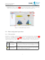
U SER M ANUAL
Version
Author
jSDN 2.0a Revision October 29, 2009
Humberto Martı́nez Barberá
jSDN Yacht Design
Contents
1 Introduction
1.1 Coordinate system . . . .
1.2 Design elements . . . . . .
1.2.1 Element classes . .
1.2.2 Element properties
1.3 Text input fields . . . . .
.
.
.
.
.
.
.
.
.
.
.
.
.
.
.
.
.
.
.
.
2 Designer Module
2.1 Module overview . . . . . . . . .
2.2 Basic and general operations . .
2.2.1 File operations . . . . . .
2.2.2 Design identification . . .
2.2.3 Printing . . . . . . . . . .
2.2.4 Other functionalities . . .
2.3 Design visualisation . . . . . . .
2.3.1 2D views . . . . . . . . .
2.3.2 3D view . . . . . . . . . .
2.3.3 Views layout . . . . . . .
2.4 Design organisation . . . . . . . .
2.4.1 Design structure . . . . .
2.4.2 Element selection . . . . .
2.4.3 Multiple element selection
.
.
.
.
.
.
.
.
.
.
.
.
.
.
.
.
.
.
.
.
.
.
.
.
.
.
.
.
.
.
.
.
.
.
.
.
.
.
.
.
.
.
.
.
.
.
.
.
.
.
.
.
.
.
.
.
.
.
.
.
.
.
.
.
.
.
.
.
.
.
.
.
.
.
.
.
.
.
.
.
.
.
.
.
.
.
.
.
.
.
.
.
.
.
.
.
.
.
.
.
.
.
.
.
.
.
.
.
.
.
.
.
.
.
.
.
.
.
.
.
.
.
.
.
.
.
.
.
.
.
.
.
.
.
.
.
.
.
.
.
.
.
.
.
.
.
.
.
.
.
.
.
.
.
.
.
.
.
.
.
.
.
.
.
.
.
.
.
.
.
.
.
.
.
.
.
.
.
.
.
.
.
.
.
.
.
.
.
.
.
.
.
.
.
.
.
.
.
.
.
.
.
.
.
.
.
.
.
.
.
.
.
.
.
.
.
.
.
.
.
.
.
.
.
.
.
.
.
.
.
.
.
.
.
.
.
.
.
.
.
.
.
.
.
.
.
.
.
.
.
.
.
.
.
.
.
.
.
.
.
.
.
.
.
.
.
.
.
.
.
.
.
.
.
.
.
.
.
.
.
.
.
.
.
.
.
.
.
.
.
.
.
.
.
.
.
.
.
.
.
.
.
.
.
.
.
.
.
.
.
.
.
.
.
.
.
.
.
.
.
.
.
.
.
.
.
.
.
.
.
.
.
.
.
.
.
.
.
.
.
.
.
.
.
.
.
.
.
.
.
.
.
.
.
.
.
.
.
.
.
.
.
.
.
.
.
.
.
.
.
.
.
.
.
.
.
.
.
.
.
.
.
.
.
.
.
.
.
.
.
.
.
.
.
.
.
.
.
.
.
.
.
.
.
.
.
.
.
.
.
.
.
.
.
.
.
.
.
.
.
.
.
.
.
.
.
.
.
.
.
.
.
.
.
.
.
.
.
.
.
.
.
.
.
.
.
.
.
.
.
.
.
.
.
.
.
.
.
.
.
.
.
.
.
.
.
.
.
.
.
.
.
.
.
.
.
.
.
.
.
.
.
.
.
.
.
.
.
.
.
.
.
.
.
.
.
.
.
.
1
2
2
2
4
4
.
.
.
.
.
.
.
.
.
.
.
.
.
.
7
7
8
8
10
11
14
15
15
17
22
23
23
24
25
A Introduction to NURBS
27
B Platform and OS specifics
B.1 MacOS X Specifics . . . . . . . . . . . . . . . . . . . . . . . . . . . . . . . . . . .
B.1.1 General usage . . . . . . . . . . . . . . . . . . . . . . . . . . . . . . . . . .
B.1.2 Printing . . . . . . . . . . . . . . . . . . . . . . . . . . . . . . . . . . . . .
31
31
31
32
C IGES support
33
i
jSDN Yacht Design
ii
jSDN Yacht Design
Introduction
Chapter 1
Introduction
jSDN is a NURBS based yacht modelling and analysis software. While it is based on and is
a follow up of the former SDN, it has been redesigned and recoded from scratch and includes
many new functionalities and much more accurate calculations, which has been and are being
validated with real designs. The main goal of jSDN is to allow the designer to fast prototype
any kind of sailing yacht, including elements like hull, spars, sails and appendages. Although it
is not limited to sailing boats, both the working procedure and tools are targeted and optimised
for those. jSDN is comprised of the following modules:
Icon
Module
Designer
Hydro
Performance
Description
Module that allows the modelling of the different elements
of the design. It includes a full NURBS curves and surfaces
editor.
This module, also referred as lines processing module (LPP),
is used to perform naval architecture calculations, wich
include hydrostatics, KN curves, and longitudinal and
transversal GZ curves.
This module, also referred as velocity prediction program
(VPP), uses aero and hydrodynamic models in order to perform a performance prediction of a given hull and sail geometry.
Tabla 1.1: jSDN modules
The Hydro and Performance modules can be executed either standalone or from within the
Designer module. In the later case, they use as input the current design of the editor.
For the interaction with other CAD systems, jSDN supports importing objects from and
exporting objects to different 3D formats like: IGES, DXF, STL, 3DS, AC3D, VRML.
1
jSDN Yacht Design
Introduction
1.1
Coordinate system
The jSDN environment makes use of the standard Naval Architecture coordinate system, as
shown in figure 1.1.
Figure 1.1: jSDN coordinate system
Unless otherwise specified, the default waterplane is assumed to be the XY plane at z = 0.
This can be modified for hydrostatic calculations.
Three different 2D projections and views are defined and used in jSDN, as described in table
1.2.
Projection
Top
Front
Side
Description
Looking from below, starboard above the centreline (XY axis).
Looking forward from the stern (YZ axis).
Looking from starboard, bow to the right (XZ axis).
Tabla 1.2: 2D projections
1.2
1.2.1
Design elements
Element classes
jSDN supports different geometric elements for modelling. Currently, the jSDN editor fully supports NURBS curves and surfaces (see appendix A for an introduction) and allows partial edition
of lines and polygonally defined surfaces.The elements of a design can be organised hierarchically, allowing grouping, which makes manageable large designs. Geometric transformations
(translation, rotation, or scaling) can be applied to all types of elements. jSDN supports the
following element classes:
• Group. This element is a container of different element types, including other group
2
jSDN Yacht Design
Introduction
elements (figure 1.3a). This allows for an effective hierarchical organisation of a design.
When a geometrical transformation is applied to a group element, it is effectively applied
to any of the elements that it contains.
• NURBS Curve. This element represents a NURBS curve (figure 1.2a), which can be
modified by varying the control points coordinates. Specific operations include: degree
elevation, knot reduction, tessellation, curve sweeping and delaunay triangulation.
• NURBS Interpolation Curve. This element represents a NURBS curve (figure 1.2b),
which can be modified by varying the interpolation points coordinates. jSDN automatically
computes the NURBS curve control points that interpolate the specified points. The
specific operations are similar to standard NURBS curve elements.
• NURBS Surface. This element represents a NURBS surface (figure 1.3b), which can
be modified by varying the control points coordinates. Specific operations include: knot
reduction, tessellation, knot transposition, and polygonal surface extraction. If specified,
NURBS surfaces can be made automatically symmetrical around the XZ plane.
• POLY Surface. This element represents a polygonal surface (figure 1.3c), lines and 3faceted and 4-faceted polyhedrals. jSDN has partial edition support of these elements.
In any case, they can be modified by varying vertexes coordinates. Specific operations
include: duplicate vertex pruning, convex hull computation, face normals inversion.
Figure 1.2: Elements a) NURBS curve b) NURBS interpolation curve
Figure 1.3: Elements a) group b) NURBS surface c) POLY surface
jSDN allows different visualisation options of the different elements. In the case of NURBS
surfaces, the control polygon can be shown or hidden, and control points can be fully shown, or
just selected U or V rows, which helps on the edition of control points.
3
jSDN Yacht Design
Introduction
1.2.2
Element properties
Each jSDN element has properties that allow to customise how the element is visualised, how the
element is edited, and finally, how the element should be treated when computing calculations
(functional properties). The following is the list of element properties:
• Name. This property is used for identifying the element in management interfaces, like
the design elements panel (see section 2.1).
• Color. This property specifies the visualisation color of the element, which is the color
used for drawing lines (wireframe) or polygons (solid or shaded). Additionally, for the
3D view, additional color related parameters can be further specified (diffuse and specular
colors, and transparency).
• Visibility. In order top help during modelling, elements can be specified to be visible or
invisible. Irrespective of the visibility state of an element, it is still listed in the design
elements panel.
• Editability. In the case of composite elements, sometimes it is desirable to treat them
as a single object, thus disallowing the edition of its internal details. This is referred as a
locked element. In other case, it is an unlocked element.
• Type/Subtype. This properties identify the main functional task of the given element.
While it is irrelevant for displaying, this allows applying specific calculations depending
on the element’s functionality. The following types and subtypes (table 1.3) are currently
supported:
Symbols
Types
HULL
Subtypes
HULL, DECK
APPENDAGE
RUDDER, KEEL, BULB
SAIL
MAINSAIL, JIB/GENOA, SPINNAKER, WINGSAIL
RIG
MAST, BOOM, POLE
PART
Tabla 1.3: Functional properties
• HullSet. This property attaches the given element to a given hull. This allows the
definition of a hull by composing different surfaces or panels. In the same way, the number
of different HullSets defines the number of hulls that will be used during calculations. If
a HullSet is not specified for a given element, it is assumed to belong to a HullSet named
Default.
1.3
Text input fields
In order to allow the designer to understand at any moment which text values (be them free
text values or numerical values) have been accepted by the program or which values are wrong
4
jSDN Yacht Design
Introduction
or outside its range, a color coding mechanism is employed. At any moment, an input text field
can be in any of the following four states:
• Accepted. When a text field is in this state (figure 1.4), the value shown is the one that
jSDN is using or will be using in its calculations. This is the default state of the text input
fields.
Figure 1.4: Text field in accepted state
• Edited. When a text field has been modified, its background color changes to yellow
(figure 1.5). In this state the changed are not acquired by jSDN until the user presses the
Intro key, in which case the input state will change to Accepted. Otherwise the value is
not known to jSDN.
Figure 1.5: Text field in edited state
• Error. In certain cases, like numerical input or ranged input, if the users types an incorrect
or out of range text, the background color changes to red, and the value shown will be the
last correct inputted value or the closest one (figure 1.6). This value is known to jSDN
and will be further used.
Figure 1.6: Text field in error state
• Disabled. A text field whose background color is grey cannot be edited (figure 1.7), and
its value is either informative or unavailable at that moment.
5
jSDN Yacht Design
Introduction
Figure 1.7: Text field in disabled state
6
jSDN Yacht Design
Designer Module
Chapter 2
Designer Module
2.1
Module overview
When jSDN Designer is executed, the main window displays as follows (figure 2.1). The main
window is divided into several panels and parts, the are described below:
• Design visualisation panels. This area (figure 2.1, caption 1) shows different views of
the design (front, top, side, three dimensions). Each view includes a toolbar that allows
to define and control its visualisation properties (see section 2.3.1 and 2.3.2). The layout
of the design view area can be modified to display a single view (either 2D or 3D) or all
the views.
• Design tree panel. This panel (figure 2.1, caption 2) shows the list of elements that
compose the design, together with a graphical representation of some of their properties.
In certain cases, this tree panel also includes a tool-specific area in the bottom. This occurs
when some element toolbars are selected (i.e. element translation).
• Toolbars. There are four toolbars, which are composed of buttons and are a handy way
of accessing to common or habitual operations with the design, the visualisation or the
current element. These toolbars are:
◦ The general toolbar (figure 2.1, caption 3.1) allows typical file and edition actions,
like saving, printing, copying, etc.
◦ The floating toolbar (figure 2.1, caption 3.2) gives access to different tools that
display their result in floating windows, like load and tank management, simple hydrostatics, etc.
◦ The modules toolbar (figure 2.1, caption 3.3) gives access to other jSDN modules
(hydrostatics, velocity prediction, optimisation, etc).
◦ The element toolbar (figure 2.1, caption 3.4) provides several tools for shaping
elements (edition, translation, rotation, scaling, etc).
• Menus. Menus (figure 2.1, caption 4) offer access to different features and commands.
Depending on the current selected element, different menus are enabled or disabled.
7
jSDN Yacht Design
Designer Module
• Status bar. This area (figure 2.1, caption 5) shows the design coordinates of the cursor
in the active view, and positioning information of the different element tools.
Figure 2.1: Main jSDN Designer window
2.2
2.2.1
Basic and general operations
File operations
Standard project and file operations can be accessed either from the general toolbar (figure 2.1,
caption 3.1), or the File menu (figure 2.1, caption 4), or through keyboard shortcuts. These
operations are described in table 2.1. The main window always shows the name of the current
design file (right after the window title, between brackets), relative to the program directory.
Tool
Submenu
New Design
Load Design
Description
Creates a new design, sets the current design name to untitled.sdn, erases all design-dependent information, and clears
the design views. It keeps the current visualisation properties.
Opens a file dialog in order to select the desired design. Then
clears the existing design, starts using the newly loaded design, and updates the design views.
Continued on next page
8
jSDN Yacht Design
Designer Module
Tool
Submenu
Merge Design
Save Design
Save Design As
Import
Export
Continued from previous page
Description
Opens a dialog in order to select the design that will be
merged. After design selection, a element selection dialog appears, which allows to specify which elements are to
be merged (see section 2.4.3 for usage information). Then,
these selected elements are incorporated into the current design, and the design views are updated accordingly.
Saves the current design with its current file name (the one
that is shown in the window title bar).
Opens a file dialog in order to select a name for the current
design. Then, it saves the design with the desired file name.
After selection of the desired format, it opens a file dialog in
order to select the desired file. The file is imported and converted into jSDN format, and the resulting design is merged
to the current one in a new GROUP element with the name
of the imported design. The design views are updated accordingly.
After selection of the desired format, it opens a file dialog
in order to select a name for the exported design. Then, it
exports the design with the desired file name.
Tabla 2.1: File operations
Some of the previously described actions are destructive (like New Design, Load Design,
Quit), that is, the current design will be lost after issuing the action. In those cases, the editor
displays an alert (figure 2.2) in order to remind the user of this situation, and allows the user
to reconsider the action (Cancel option), save the current design (Save option), or discard the
command (Discard option).
Figure 2.2: Design modified alert
The list of supported import/export formats is presented in table 2.2. For each format
it shows whether import or export is supported and some format-relevant information. See
appendix C for a more detailed description of IGES support.
9
jSDN Yacht Design
Designer Module
Format
IGES 5.3
IMS Offsets
MARNET Offsets
STL
VRML 2.0
3DS
AC3D
DXF R14
Import
x
x
x
x
x
x
x
x
Export
x
Comment
Standard format for CAD exchange.
ORC hull offsets file format.
Hull format of the MARNET-CFD database.
Standard for stereo lithography rapid prototyping.
Standard format for 3D web publishing.
AutoDesk 3D Studio file format.
Inivis AC3D file format.
AutoDesk AutoCAD file format.
Tabla 2.2: Import and export file formats
2.2.2
Design identification
jSDN keeps some information related to the design, to be later displayed in certain operations.
When a new design is created, all the information fields are empty. Although it is not required,
it is strongly recommended to fill this fields. They can be modified using the menu Project →
Design Info. This menu opens a dialog window as shown in figure 2.3.
Figure 2.3: Design information dialog
The information introduced in this dialog is not parsed by jSDN, which means the user is
free to use the fields at his/her will. Moreover, jSDN does not check text length boundaries, and
so the user has to trim the text depending on its use. The operations where this information is
used are:
• Printing. All CAD-printing operations draw a box on the bottom-right side of the paper,
which includes all the project information. The information introduced in the dialog shown
in figure 2.3 is printed as shown in figure 2.4. See section 2.2.3 for more information.
Figure 2.4: Design information in printing
10
jSDN Yacht Design
Designer Module
• Calculations. Calculation modules (hydrostatics, velocity prediction, etc) create a report
which contains a header with the project information, as shown in figure 2.5. See next
chapter for more information.
Figure 2.5: Design information in hydrostatics
2.2.3
Printing
Printing operations can be accessed either from the general toolbar (figure 2.1, caption 3.1),
or the File menu (figure 2.1, caption 4), or through keyboard shortcuts. These operations are
described in table 2.3.
Tool
Submenu
Page Setup
Print Preview
Description
Opens a dialog that allows to configure general options of the
printing process: paper size, paper orientation, etc. These
options are kept for later use while printing. The actual
appearance of this dialog depends on the current operating
system (see appendix B for your specific OS).
Opens the Print Preview window which allows the user to
specify which portions of the design are to be printed and
in which format, before actually printing the design.
Tabla 2.3: Print operations
The Print Preview window is shown in figure 2.6. It includes its own menu bar, with three
menus: a File menu, which includes the printing operations described above, a View menu,
which includes 2D options of the View menu of the main window (see section 2.3.1), and the
Window menu (see section 2.2.4).
The Print Preview window shows a three-view projection of the current printing selection,
rendered with the current 2D rendering method, as selected in the View menu. The window
includes a text input field named Comment, which allows the user to enter as text which will
be printed just under the design name, in the info box, as shown in figure 2.4. If no text is
introduced (that is, the text field shows the ’N/A’ value), nothing is printed under the design
11
jSDN Yacht Design
Designer Module
namae. In the bottom-right corner of the window, there is a button which sends the print job
to the printer. After pressing the button, the design shown in figure 2.6 is printed as shown in
figure 2.7.
Figure 2.6: Print Preview window
12
jSDN Yacht Design
Designer Module
Figure 2.7: Actual printing output
13
jSDN Yacht Design
Designer Module
2.2.4
Other functionalities
14
jSDN Yacht Design
Designer Module
2.3
Design visualisation
A jSDN design can be displayed using a combination of powerful 2D and 3D views, that can
be combined in different ways. The following sections describe the 2D and 3D views, and their
onscreen layouts.
2.3.1
2D views
The 2D projection panels are as shown in figure 2.8. These views allow several customisation
and commands in order to change global appearance, rendering, point of view, edition and the
like. All of them are described in this section.
Figure 2.8: 2D design panel
The projection views can be configured to render the elements in one of the three different
modes described below. Depending on the design task we are performing, a rendering mode
or other can be more suitable. All 2D projections use the same rendering mode, it is a global
property to all of them. This property can be changed at any time with the menu View →
2D Rendering, and it is persistent from session to session. It is stored in the editor.conf
configuration file.
• The wireframe mode (figure 2.9) displays elements using lines in the element’s color.
This is the fastest rendering method, and the only responsive enough when running on
slow processors. Use menu item View → 2D Rendering → Wireframe to select this
mode.
• The solid mode (figure 2.10) displays elements using polygons of the element’s color. This
rendering is a little bit slower than wireframe, but, on the other hand, it implements what
is called a z-buffer, that is, elements closer to the observer are drawn on top of those
further. Use menu item View → 2D Rendering → Solid to select this mode.
• The shaded mode (figure 2.11) displays elements using polygons of the element’s color,
but taking into account lighting. This rendering is much slower than wireframe, and should
15
jSDN Yacht Design
Designer Module
Figure 2.9: Wireframe drawing mode
Figure 2.10: Solid drawing mode
be used on fast processors. It implements what is called Gouraud shading in addition to
the z-buffer, which allows displaying ordered polygons in different shades. Use menu item
View → 2D Rendering → Shaded to select this mode.
Figure 2.11: Shaded drawing mode
Each visible projection view includes its own toolbar and a display area, which is used for
editing elements. The toolbar (table 2.4) has the following options, which may be enabled or
disabled depending on the current selected element:
Tool
Description
When this tool is selected, the panel is in editing mode. In this mode, any
mouse movement or left-button click will be processed by the current
element tool (figure 2.1, caption 3.4).
This tool allows to pan the current design view in conjunction with a
left-click. No edition is performed.
This tool allows to zoom in or zoom out in conjunction with a left-click.
No edition is performed.
This tool changes the current zoom in order to include the full visible
part of the whole design.
Continued on next page
16
jSDN Yacht Design
Designer Module
Tool
Continued from previous page
Description
This tool is only active with depth-ordered rendering, as in solid
or shaded rendering.
Changing the state of the button (selected/unselected) modifies the ordering of the polygons, that is, showing
on top those closer to the observer or those further from the observer.
This tool enables/disables displaying the control net or control curve
in NURBS surfaces and curves. It is only available with these kind of
elements.
This tool enables/disables displaying the derivatives of the current
NURBS curve or surface. It is only available with these kind of elements.
This tool enables/disables displaying a reference grid in the design area.
This grid dynamically adapts to the extent of the zoom, and includes
the coordinates of the grid lines
This tool changes the control point visualisation style for the current
NURBS surface. If no NURBS surface is selected, the tool is disabled.
There are three possible options:
• All. Shows all the NURBS surface control points.
• V Row. Enables V-only control point displaying. This is the
typical ordering of longitudinal rows of control points in a jSDN
created hull.
• U Row. Enables U-only control point displaying. This is the
typical ordering of transversal columns of control points in a jSDN
created hull.
This tool allows the selection of the current U or V row of control points.
It is only enabled for NURBS surfaces.
Tabla 2.4: 2D projection toolbar
2.3.2
3D view
The 3D view panel is as shown in figure 2.12. This view allows several customisation and
commands in order to change global appearance, lighting, point of view, coloring and the like.
All of them are described in this section.
The 3D view can be configured to render the elements in one of seven different coloring
modes described below. The 3D coloring property can be changed at any time with the menu
View → 3D Coloring.
• The design mode is the default coloring mode, which renders each element with is userdefined color. Use menu item View → 3D Coloring → Design Colors to select this
mode. This is the default 3D coloring mode.
• The checkers mode (figure 2.13) renders each element using a checkers pattern based on
17
jSDN Yacht Design
Designer Module
Figure 2.12: 3D design panel
the element’s design color. Use menu item View → 3D Coloring → Checkers Pattern
to select this mode.
Figure 2.13: Checkers pattern coloring
• The curvature mode renders each element using shades of colors which represent values of
the discrete surface curvature at each point. A surface is typically curved in two directions,
called the principal curvatures, P C1 and P C2 . Depending on how these curvatures are
combined, there are different curvature displays, which are selected in the menu View →
3D Coloring → Curvature. Curvature coloring is only available to NURBS surfaces.
For any other type of element, the design colors are used instead. The different curvature
options are described below.
The Gaussian mode (figure 2.14) shows the Gaussian curvature at each point
of the surface, which is computed as the product of the two principal curvatures
P C1 × P C2 . Use menu item View → 3D Coloring → Curvature →Gaussian
to select this mode. The Gaussian curvature is very important for assessing
surface developability, and, although it is not a direct measure of it, for checking
surface fairness. Gaussian curvatures are shaded as one of either of three colors:
◦ Blue corresponds to negative values of the Gaussian curvature, presenting the shape of a saddle. In this case the curvature is positive in one
direction and negative in the other.
◦ Red corresponds to positive values of the Gaussian curvature, representing convex or concave shapes. In this case either both curvatures are
positive of both are negative, that is, both have the same sign.
18
jSDN Yacht Design
Designer Module
◦ Green corresponds to a zero value of the Gaussian curvature, representing surfaces that are flat or curved in one direction. In this case one
principal curvature must be zero, while the other can have any value.
This is a condition for developable surfaces.
Figure 2.14: Gaussian curvature coloring
The mean curvature mode (figure 2.15) shows the mean curvature at each point
of the surface, which is computed as the average of both principal curvatures
(P C1 + P C2 ) × 0.5. Use menu item View → 3D Coloring → Curvature →
Mean Curvature to select this mode.
Figure 2.15: Mean curvature coloring
The principal curvature 1 mode (figure 2.16) shows the transversal curvature
P C1 at each point of the surface. Use menu item View → 3D Coloring →
Curvature → Principal Curvature 1 to select this mode.
Figure 2.16: Principal curvature 1 coloring
The principal curvature 2 mode (figure 2.17) shows the longitudinal curvature
P C2 at each point of the surface. Use menu item View → 3D Coloring →
Curvature → Principal Curvature 2 to select this mode.
The surface element mode (figure 2.18) shows the surface element curvature
at each point of the surface, which is computed as the norm of the dot product
of both curvature vectors k P~C1 · P~C2 k. Use menu item View → 3D Coloring
→ Curvature → Surface Element to select this mode.
The 3D view includes a toolbar which allows to control the visualisation of the elements, as
described in table 2.5.
19
jSDN Yacht Design
Designer Module
Figure 2.17: Principal curvature 2 coloring
Figure 2.18: Surface element coloring
Tool
Description
This tool allows to pan the current design view horizontally in conjunction with a left-click.
This tool allows to pan the current design view vertically in conjunction
with a left-click. No edition is performed.
This tool allows to rotate the design in conjunction with a left-click.
The center of rotation is the current point of view. It can be changed
by panning either vertically or horizontally.
This tool allows to zoom in or zoom out in conjunction with a left-click.
Zooming is achieved by separating or getting close to the current point
of view. Because of the rendering engine, there is a limit on how close
to the view point we can get. Parts of objects behind the eye point are
not displayed.
This tool changes the current zoom in order to include the full visible
part of the whole design.
This tool opens a preferences floating panel that allows the configuration
of some parameters of the 3D view, like lighting, sea texture, rotation
method, etc.
This tool enables/disables displaying the control net or control curve
in NURBS surfaces and curves. It is only available with these kind of
elements.
This tool enables/disables displaying the derivatives of the current
NURBS curve or surface. It is only available with these kind of elements.
This tool enables/disables displaying a reference grid in the design area.
This grid dynamically adapts to the extent of the zoom, and includes
the coordinates of the grid lines
Continued on next page
20
jSDN Yacht Design
Designer Module
Tool
Continued from previous page
Description
This tool changes the control point visualisation style for the current
NURBS surface. If no NURBS surface is selected, the tool is disabled.
There are three possible options:
This tool allows the selection of the current U or V row of control points.
It is only enabled for NURBS surfaces.
This tool allows the selection of the current U or V row of control points.
It is only enabled for NURBS surfaces.
Tabla 2.5: 3D view toolbar
When the preferences toolbar button is selected, a floating panel appears as shown in figure
2.19. The panel can be later hidden by unselecting the button or by closing the panel. This
panel presents four different sections:
• Lighting properties. The 3D view is lighted by three independent directional lights and
an ambient light source. These can be enable or disabled. For each enabled light source,
its intensity can be modified so that it is brighter or darker.
• Viewing options. These options allows displaying viewing aids, like the 3D reference
axis, the surface grid (whose size and extent can be customised with two text fields),
and the surface texture (which can be selected from several available in the combo box).
The light sources can be displayed and are represented as white spheres. By default light
sources are not rotated with the design. But they can be selected to do so.
• Curvature options. This option allows changing the brightness of the curvature rendering. The practical effect of this control is to modify the contrast between the three
curvature shades (red, green, blue).
• Input options. For 3D rotation control there are two control methods, which are described below. Both methods rotate the current design with respect to the current point
of view. This can be modified by way of translation (either horizontal or vertical).
Elevation-Azimuth. This input method independently controls the elevation
(vertical mouse movement) and azimuth (horizontal mouse movement) angles.
The azimuth control is continuous (the design can be rotated indefinitely both
clockwise or counter-clockwise), while the elevation control is limited to ±90◦
degrees. This is the default rotation method.
ArcBall. This input method couples elevation and azimuth angle change by
mapping the on screen mouse movement onto a sphere. In this case both azimuth
and elevation control is continuous. While this mode allows for easily reaching
any face of the design, it is however much more responsive, and thus it is not
easy to fine-tune rotation control.
21
jSDN Yacht Design
Designer Module
Figure 2.19: 3D preferences floating panel
2.3.3
Views layout
Three methods are available in jSDN to change the layout of the design views: using the main
menu (figure 2.1, caption 4), using the general toolbar (figure 2.1, caption 3.1), and using
keyboard shortcuts. This allows for a quick change between views as needed during the design
tasks. The different layouts are summarised in table 2.6, including their corresponding menus,
tool icons and shortcuts. By default, a four view is used.
Layout
All views
Front view
Top view
Side view
3D view
Menu
View →
View →
View →
View →
View →
Toolbar
Layout
Layout
Layout
Layout
Layout
→
→
→
→
→
All views
Front view
Top view
Side view
3D view
Tabla 2.6: Design views layout
22
Keyboard shortcut
F1
F2
F3
F4
F5
jSDN Yacht Design
Designer Module
2.4
Design organisation
A central and important tool in the design activity is the design tree, which is shown in figure
2.20. This tree panel is a floating toolbar that, by default, is located on the left side of the jSDN
Editor window. At any time it can be dragged out of that position and be situated floating over
any portion of the screen, allowing a larger view of the visualisation panels. It can be positioned
back into its normal state by pressing the close button of the floating panel. The functionalities
of the design tree are described in the following subsections.
Figure 2.20: Design tree panel
2.4.1
Design structure
The tree shows the structure of the current design and properties of the elements that constitute
it. Elements are displayed each in a different row, and are arranged so that they are indented
by tree levels: elements closer to the left side of the panel are placed higher in the design
hierarchy, while elements closer to the right side of the panel are placed lower in the hierarchy.
Because the hierarchy is organised through GROUP elements, these are identified with the
icon. GROUP elements that are editable and contain elements include tree handles that allow
to collapse ( ) or expand ( ) their corresponding subtrees. Clicking on a handle changes the
state from collapsed to expanded and vice-versa. Tree collapsing and expanding is independent
of the visibility property of the elements.
Each tree element is identified by its name, and each row also includes a graphical representation of some of their properties, in the following order:
• Visibility. Shows whether the element is visible
or not .
• Editability. Shows whether the element is editable
• Color. Shows the design color of the element .
23
or not
.
jSDN Yacht Design
Designer Module
• Type. Shows the type of the element using its icon
,
, ...
The tree structure can be modified at any time by drag and drop operations. In order to
drag an element, first select it by pressing left button onto the corresponding tree row, and
without releasing the button move the mouse over the tree. When the mouse reaches the top
or bottom part, the tree is automatically scrolled. In order to drop the element, simply release
the left button.
2.4.2
Element selection
The tree also show the current element, that is, the element that can be edited and can receive
edition tool commands, and so it is reflected in the 2D panels. The selected element is shown
in the tree with a blue background and the element name in red. This element is also drawn in
the 2D panels with a yellow box around it and some handles to edit or modify the element.
The design tree implements contextual menus for the selected element. These contextual
menus include information and operations that can be performed over the selected element, like
changing element’s name or editing its properties. A contextual menu displays after pressing the
right button, as shows figure 2.21. Actions are then selected as in normal menus, by pressing left
button. The contextual menu is divided into different sections, and offers the following options:
Figure 2.21: Design tree contextual menu
• The first sections displays information relative to the selected element as: element class
(NURBS curve, NURBS surface, etc), number of vertexes (only for group and POLY
elements), and type, subtype and hullset properties.
• The next section includes standard edition operations as: copy, cut and paste.
• The next section allows the modification of different element properties as: name, type
and subtype, hullset and color.
24
jSDN Yacht Design
Designer Module
• The last section graphically displays whether the element visibility and editability properties.
2.4.3
Multiple element selection
In certain operations, like design merging or multiple element deleting, the user has to select
a number of elements from either the current or an external jSDN design file. In these cases,
the editor displays a multiple element selection window (figure 2.22). The window is divided in
two parts: the upper one shows three 2D views (see section 2.3.1) and one 3D view (see section
2.3.2), while the lower one shows an element selection table. Independently of the current user
selection, the 2D views are configured in wireframe mode. The selection table shows all the
elements that are not of class GROUP, and for each element, the most relevant properties are
shown: visibility state, name, color, type/subtype, and class. In addition to these, each element
also includes a check box in order to include (selected) or exclude (unselected) the element
from the selection. When an element row is selected, by left clicking on the row, the element
is shown in the upper part views. The window includes commodity buttons for speeding up
selection operations: Select All button, selects all element in the table, and Select None
button, unselects all elements in the table.
Figure 2.22: Multiple element selection window
25
jSDN Yacht Design
Designer Module
26
jSDN Yacht Design
Introduction to NURBS
Appendix A
Introduction to NURBS
A three-dimensional object is made up of curves and surfaces. Common methods of representing
curves and surfaces are the implicit method and the parametric method. The implicit method
utilizes a mathematical function which depends on the variables of the axes, and is even to zero.
It describes a relation between the different variables from the axes. For example, the function:
f (x, y) = x2 + y2 − 1 = 0
(A.1)
In the parametric method, each variable is a function of an independent parameter. Here,
curves could be defined with the independent variable such as:
C(u) = (x(u), y(u)) , a ≤ u ≤ b
(A.2)
In order to represent the first quadrant of a circle in parametric form, we can write in several
forms, for example
C(u) = (cos u, sin u) , 0 ≤ u ≤ π/2
(A.3)
or as
C(u) =
1 − u2
2u
,
2
1 + u 1 + u2
!
,0 ≤ u ≤ 1
(A.4)
That is to say, the representation of a curve in parametric form is not unique.
A parametrical class of curves and surfaces are Non-Uniform Rational B-Spline (NURBS).
NURBS are desirable for computational reasons, because of the ease of processing by a computer,
stability with regard to floating front errors, their requirement of little memory, and their ability
to represent a wide variety of curves and surfaces. NURBS are the generalization of nonrational
B-Splines, which are based on the Bezier rational curves. These in turn are a generalisation of
Bezeir curves. The important characteristics of Bezier curves are:
27
jSDN Yacht Design
Introduction to NURBS
• Control polygons may be used to control the curves.
• The extreme control points agree with the value of the curve for u = 0 and u = 1.
• The tangent in P0 and Pn are parallel to P0 − P1 and Pn−1 − Pn .
The problem with Bezier curves is that they are not able to represent conical cambers (curves
originating from the cut of a cone with a plane). Conical cambers can however be represented
using a rational functions, defined as the quotient between two polynomials according to
x(u) =
Y (u)
Z(u)
X(u)
=
=
W (u)y(u)
W (u)z(u)
W (u)
(A.5)
wi may be interpreted as scalable weights. When the weights are varied, control points may
attract/repulse the curve. A curve formed by a single segment of a rational Bezier curve is
often inadequate. A single segment requires a high degree to define a complex form, which is
inefficient to process, and numerically unstable.
Curves using single segments have limitations in making local forms. This is solved by
defining the curve in pieces. A Bezier curve or a B-Spline when formed by pieces is constructed
with several curves united at points of rupture with continuity of alignment between them.
To create points of rupture in B-Splines one inserts knots in them. A sequence of knots form
a vector of knots, and is defined by U = u0 , . . . , um , which must fulfill that it is a sequence of
nondecreasing numbers; that is to say, ui ≤ ui+1 for all i = 0, . . . , m. The knots are, therefore,
where the curve parts connect.
In Figure A.1, one may observe the knots of the curve (u0 , u1 , u2 , u3 ), the parts into which
curve is divided (C1 (u), C2 (u), C3 (u)), the control points (open circles at the ends of the curves)
and control polygons (formed by the straight lines joining the control points).
Figure A.1: B-Spline Curve
We are introducing now the minimum parameters needed to work with this kind of surfaces.
The working surfaces are NURBS, although the program at the moment does not allow modification of the distribution of knots; these are redistributed nonuniformly when control points
are inserted or eliminated. NURBS curves have four fundamental elements in their definition:
control points, weights, knot vectors, and degree (in general, one only speaks of the degree of
functions with orders greater than one):
28
jSDN Yacht Design
Introduction to NURBS
• Control points define an approach to the curve. These control points are capable of
being moved in space, and thus can modify the form of the surface. The control points
form a vector of points if it is a curve, and together in the established order form a denoted
a control polygon. Control polygons have an important property that the designer must
understand: all the points are on the curve.
• Weights correspond mathematically to the homogeneous coordinates in a space of four
dimensions (x, y, z, w), present in each curve and rational surface. The associated weights
are at the control points. Intuitively, the greater the weight of a control point, the greater
the attraction that point exerts on the curve. The increase (or decrease) in weight produces
a change in approach (distance) to the associated control point. A weight value does not
modify the curve with respect to the nonrational curve. With weight values greater than
one, the curve approaches the control point. With values smaller than one, the curve moves
away, with the limit being a straight line uniting the points before and after the control
point. One does not normally work with negative weights. Together the modification of
weights and control points allows to local modifications of the curves and surfaces.
• The knot vector divides the curve in parts so that the base functions (functions defining
the curve) are amplified according to the interval between knots and where they are located.
If a curve is a B-Spline, it by definition has all its knots uniformly distributed. A NURBS
is a Non Uniform Rational B-Spline; that is to say, it is a B-Spline that being rational
implies that it has weights and can be acted on them, and that its knots are not distributed
uniformly. If it is a curve, single a vector of knots in the direction or when is a surface,
work with two vectors U and V, one for each direction. These directions are parametrical,
so that the directions in 3D space are defined by the control points.
• The degree of the curve indicates if it is linear, parabolic, quadratic, etc. To a great degree,
maintaining the polygon points of constant control, the curve smoothes more with respect
to the control polygon, being degree the zero points of control and degree the one polygon
of control.
It is important to note that modifying the position of a control point produces a local
modification of the surface. The area affected by this modification is given by the degree of the
surface and the location of other control points, if the vector knots stay unchanged. That is, it is
possible to modify an area by inserting rows and columns of control points in the area, and later,
moving the points as necessary. When inserting new control points, the curve remains invariant;
nevertheless, eliminating control points causes variations in the curve, allowing a resulting curve
very different from the initial curve.
29
jSDN Yacht Design
Introduction to NURBS
30
jSDN Yacht Design
Platform and OS specifics
Appendix B
Platform and OS specifics
jSDN has been developed using the Java 1 programming language, so that it can be run on many
operating systems and hardware platforms. Current jSDN has been tested and works correctly
in the configurations shown in table B.1 (this does not prevent jSDN from working on other
OS/platform combination).
Operating System
Apple OSX 10.5.6
Apple OSX 10.4.11
Windows Vista
Windows XP SP3
Processor
Intel CoreDuo
PPC G4
Intel CoreDuo
AMD Athlon
Java Virtual Machine
JDK 1.5.0
JDK 1.5.0
JDK 1.6.0
JDK 1.6.0
Tabla B.1: jSDN tested platforms
Although the operation and use of jSDN is similar on the different platforms, there are
small and minor differences between them. The following sections introduce and describe those
differences.
B.1
B.1.1
MacOS X Specifics
General usage
When jSDN Designer is executed under the MacOS X operating system, the screen looks like
figure B.1. One characteristic of the MacOS X system is that the menu bar of the applications
is always placed on the top part of the screen, and it is switched or replaced when a different
application is focused (a focused application is the one with the user input). In addition,
applications include a menu with the name of the application (actually, it is the first menu in
the menu bar). This menu is named jSDN, and includes standard Apple submenus together
with an About submenu, which opens the about dialog, and the Quit submenu, which exists
the application (in the MacOS X version, the File menu does not contain the Quit submenu).
1
http://java.sun.com
31
jSDN Yacht Design
Platform and OS specifics
Figure B.1: MacOS X main window
While MacOS X supports most 1, 2, and 3-button mouses, many of the standard Apple
mouses only have a button. The typical action of the button corresponds to a left click. There
are some operations in jSDN that require a right click. These can be performed on theses mouses
by clicking the single button while pressing the control key on the keyboard. This is a standard
MacOS X functionality.
B.1.2
Printing
The page setup dialog on MacOS X is as shown in figure B.2.
Figure B.2: MacOS X page setup dialog
32
jSDN Yacht Design
IGES support
Appendix C
IGES support
IGES1 stands for Initial Graphics Exchange Specification, and defines a neutral (that is, vendor
independent) data format that allows the digital exchange of information among Computer-aided
design (CAD) systems. The official title of IGES is Digital Representation for Communication of
Product Definition Data, first published in January, 1980 by the National Bureau of Standards
as NBSIR 80-1978. Many documents (like the Defense Standards MIL-PRF-28000B and MILSTD-1840C) refer to it as ASME Y14.26M, the designation of the ANSI committee that approved
IGES Version 1.0.
After the initial release of STEP (ISO 10303) in 1994, interest in further development of IGES
declined, and Version 5.3 (1996) was the last published standard, and it is the one supported in
jSDN. A decade later, STEP has yet to fulfill its promise of replacing IGES, which remains the
most widely used standard for CAD interoperability.
The fundamental unit of data in the file is the entity. Entities are categorized as geometry
and non-geometry. Geometry entities represent the definition of the physical shape and include
points, curves, surfaces, solids, and relations which are collections of similarly structured entities.
Non-geometry entities typically serve to enrich the model by providing a viewing perspective
in which a planar drawing may be composed and by providing annotation and dimensioning
appropriate to the drawing. Non-geometry entities further serve to provide specific attributes
or characteristics for individual or groups of entities and to provide definitions and instances for
groupings of entities. The definitions of these groupings may reside in another file. Typical nongeometry entities for drawing definition, annotation, and dimensioning are the view, drawing,
general note, witness line, and leader. Typical non-geometry entities for attributes and groupings
are the property and associativity entities.
An IGES file is composed of 80-character ASCII records, and consists of different sections:
Start, Global, Directory Entry, Parameter Data, and Terminate. The IGES standard defines a
large number of entity types. jSDN support a number of IGES entities, most of them related
to NURBS curves and surfaces and data organisation. Table C.1 shows which IGES entities are
available either for import or export operations.
The IGES support is geometrically closed with respect to jSDN designs (only NURBS curves
1
http://ts.nist.gov/standards/iges/
33
jSDN Yacht Design
IGES support
Entity
100
102
110
120
126
128
141
143
308
314
406
408
Import
x
x
x
x
x
x
x
x
x
x
x
x
Export
x
x
x
x
x
x
Description
Circular arc
Composite curve
Line
Surface of revolution
Rational B-spline curve
Rational B-spline surface
Boundary entity
Bounded surface
Subfigure definition entity
Color definition entity
Property entity
Singular subfigure instance entity
Tabla C.1: Supported IGES entities
and surfaces): if a design is exported to IGES and then reimported to jSDN, the user obtains a
geometrically identical design: element types and color properties are preserved. Unfortunately,
element properties but color are not preserved (like visibility, type, etc). While importing,
element properties are set to their default values (visible, editable, HULL, default hullset, etc).
When a design is exported as IGES, a dialog is displayed (figure C.1) which allows the
user to fine-tune the export process. The user can select how the design hierarchy is exported.
By default elements are exported as a flat structure (no hierarchy). If the option is selected,
elements in a group are exported as a 308 entity, which allows to preserve the hierarchy. Use
this option depending on the program you will be importing the design to. In the particular
case of symmetrical NURBS surfaces, they are exported as two different elements: the original
element and its symmetrical (renamed with the base name and the ’SYM ’ suffix).
Figure C.1: IGES export options dialog
34