Download MICHPAVE User`s Manual - Michigan State University

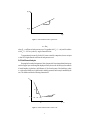
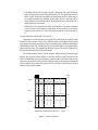
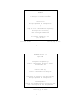
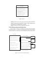
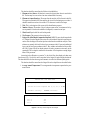
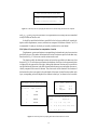
MICHPAVE
User’s Manual
(Version 1.2 for DOS)
Asphalt
Base
Roadbed
Ronald S. Harichandran
Gilbert Y. Baladi
MICHPAVE USER’S MANUAL
(Version 1.2 for DOS)
by
Ronald S. Harichandran
Associate Professor
and
Gilbert Y. Baladi
Professor
Department of Civil and Environmental Engineering
Michigan State University
East Lansing, MI 48824-1226
January 2000
 1995 Michigan State University Board of Trustees
ii
Table of Contents
1.
2.
3.
4.
5.
6.
6.
Introduction.................................................................................................................1
Summary of Modeling and Analysis ..........................................................................1
2.1
Modeling of the Pavement ........................................................................1
2.2
Granular and Cohesive Material Models ..................................................1
2.3
Gravity and Lateral Stresses .....................................................................1
2.4
Finite Element Analysis............................................................................2
2.5
Computation of Stresses and Strains at Layer Interfaces..........................4
2.6
Estimated Equivalent Resilient Moduli ....................................................4
2.7
Fatigue and Rut Depth Prediction.............................................................4
System Requirements..................................................................................................4
Configuring the Computer ..........................................................................................5
4.1
Installation Procedure ...............................................................................5
4.2
The CONFIG.SYS File.............................................................................5
4.3
Required Amount of Free Memory...........................................................5
4.4
Printing Graphics ......................................................................................5
4.5
Running MICHPAVE for the First Time..................................................6
Using MICHPAVE .....................................................................................................6
5.1
Filenames ..................................................................................................6
5.2
Cursor Movement and Editing Keys.........................................................6
5.3
Title Screen ...............................................................................................7
5.4
Main Menu................................................................................................7
5.5
Data File Menus and Associated Data-Entry Forms.................................9
5.6
Performing Analysis ...............................................................................16
5.7
Plotting the Results .................................................................................18
5.8
Printing the Results .................................................................................20
Problem Reporting ....................................................................................................20
References.................................................................................................................20
iii
List of Figures
Figure 1.
Figure 2.
Figure 3.
Figure 4.
Figure 5.
Figure 6.
Figure 7.
Figure 8.
Figure 9.
Figure 10.
Figure 11.
Figure 12.
Figure 13.
Figure 14.
Figure 15.
Figure 16.
Figure 17.
Figure 18.
Figure 19.
Figure 20.
Figure 21.
Figure 22.
Figure 23.
Figure 24.
Resilient modulus model for granular soils ................................................................2
Resilient modulus model for cohesive soils................................................................2
Typical finite element mesh........................................................................................3
Title screen..................................................................................................................8
Credits screen..............................................................................................................8
Main menu ..................................................................................................................9
Overview flowchart of the MICHPAVE program......................................................9
New data file menu ...................................................................................................10
Data-entry form for initial data .................................................................................10
Data-entry form for fatigue life and rut depth ..........................................................11
Data-entry form for layer type ..................................................................................12
Data-entry form for linear elastic (type 1) material properties ................................12
Data-entry form for granular (type 2) material properties ........................................13
Data-entry form for cohesive (type 3) material properties ......................................13
Data-entry form for specifying the number of cross sections along which
results are computed .................................................................................................14
Data-entry form for specifying the location of horizontal cross sections.................14
Data-entry form for specifying the location of vertical cross sections .....................15
Data-entry form for modifying the number of elements in the vertical
direction ....................................................................................................................16
Data-entry form for modifying the number of elements in the
horizontal direction ...................................................................................................16
Typical display during computation .........................................................................17
Typical design summary ...........................................................................................17
Plot menu for selecting sections ...............................................................................18
Menu for plots along vertical cross sections.............................................................19
Menu for plots along horizontal cross sections........................................................19
List of Tables
Table 1.
Keypad functions within data-entry forms .................................................................7
iv
1. Introduction
MICHPAVE is a user-friendly, non-linear finite element program for the analysis of flexible
pavements. The program computes displacements, stresses and strains within the pavement due to
a single circular wheel load. Useful design information such as fatigue life and rut depth are also
estimated through empirical equations.
Most of MICHPAVE is written in FORTRAN 77. Graphics and screen manipulations are
performed using the FORTRAN callable GRAFMATIC graphics library, marketed by Microcompatibles Inc., 301 Prelude Drive, Silver Spring, MD 20901.
2. Summary of Modeling and Analysis
This section gives a summary of the modeling and analysis so that the user is aware of the
capabilities and limitations of the MICHPAVE program. Further details about the modeling and
analysis, and various sensitivity studies, are given in the works by Yeh (1989), and Harichandran,
et. al. (1989, 1990).
2.1 Modeling of the Pavement
Each layer in a pavement cross section is assumed to extend infinitely in the horizontal directions, and the last layer is assumed to be infinitely deep. All the pavement layers are assumed to be
fully bonded so that no slip occurs due to applied load. Displacements, stresses and strains due to
a single circular wheel load are computed. Due to the assumptions used, the problem is reduced to
an axisymmetric one.
2.2 Granular and Cohesive Material Models
The so-called K-θ model is used to characterize the resilient moduli of granular (type 2) materials. This model is of the form
M R = K 1θK 2
in which θ = σ1 + σ2 + σ3 = bulk stress and MR = resilient modulus, and K1 and K2 are material
properties. For this model, log MR varies linearly with log θ as shown in Fig. 1.
The resilient modulus for cohesive soils is specified in terms of the deviatoric stress through
the bilinear model:
 K 2 + K 3 [ K 1 – ( σ 1 – σ 3 ) ],
MR = 
 K 2 + K 4 [ ( σ 1 – σ 3 ) – K 1 ],
when ( σ 1 – σ 3 ) ≤ K 1
when ( σ 1 – σ 3 ) > K 1
This model is illustrated in Fig. 2.
2.3 Gravity and Lateral Stresses
The MICHPAVE program includes the effect of gravity and lateral stresses arising from the
weight of the materials. At any location within the pavements, the vertical gravity stress (σg) is
computed as the accumulation of the layer thicknesses multiplied by the appropriate unit weights.
The lateral stress is taken as
1
log MR
K2
1
log K1
log θ
Figure 1
Resilient modulus model for granular soils
σh = K0σg
where K0 = coefficient of earth pressure at rest. For granular soils K0 = 1 − sin φ and for cohesive
soils K0 = 1 − 0.95 sin φ, where φ = angle of internal friction.
To approximately account for “locked-in” stresses caused by compaction, the user can input
a value for K0 higher than the coefficient of earth pressure at rest.
2.4 Finite Element Analysis
Rectangular four-noded axisymmetric finite elements with linear interpolation functions are
used in all upper layers and through the depth specified by the user for the last layer (the roadbed).
A lateral boundary is placed at a radial distance of 10a from the center of the loaded area, where
a = radius of the loaded area. A default mesh is initially generated, but this may be modified by the
user. The default mesh has the following characteristics:
MR
K3
1
K4
K2
1
σ1 − σ3
K1
Figure 2
Resilient modulus model for cohesive soils
2
• In the radial direction, the total width of 10 radii is divided into four regions. Within any
region, all elements have the same horizontal dimension. The first region, between 0 and 1
radius, is equally divided into four elements; the second region, between 1 radius and 3 radii, is equally divided into four elements; the third region, between 3 radii and 6 radii, is
equally divided into three elements; and the fourth region, between 6 radii and 10 radii, is
equally divided into two elements.
• Within any layer, all elements have the same vertical dimension. The number of elements
in each layer in the vertical direction is dependent on the layer thickness, but at least four
elements are used in the top (AC) layer, and at least two elements are used in all other layers.
A typical default finite element mesh is shown in Fig. 3.
Displacements, stresses and strains are computed only within the region modeled by finite
elements. In order to increase accuracy, and to reduce the memory and computation time required
by the program, the infinite extent of the last layer is modeled by using a flexible bottom boundary
(Harichandran and Yeh 1989). The half-space below the bottom boundary is assumed to be homogeneous and linear elastic. The modulus of the half-space is taken as the average moduli of the finite elements immediately above the bottom boundary.
The non-linear analysis consists of several iterations. A linear analysis is performed in each
iteration, after which the resilient modulus of each finite element is revised if necessary. If the
Mohr-Coulomb failure criterion is violated in any granular or cohesive soil element, then the principal stresses are modified to reflect the failure condition, and the resilient moduli are determined
from the modified stresses (Raad and Figueroa 1980). The iteration is repeated until the resilient
moduli of all the elements stabilize.
Depth
0.0"
Asphalt
10.0"
Base
30.0"
Roadbed
0
a
3a
6a
50.0"
10 a
Radial Distance in Radii (Radius of loaded area, a = 5.35 in.)
Figure 3
Typical finite element mesh
3
2.5 Computation of Stresses and Strains at Layer Interfaces
For the interpolation functions used in the finite element approach, stresses and strains are
most accurate at the center of elements. The following techniques are used to obtain improved estimates of some stresses and strains at layer interfaces:
• The vertical stress is obtained from the vertical stresses at the center of the two elements
above and the two elements below the interface by using cubic interpolation.
• The radial, tangential and shear stresses and vertical strain are obtained using extrapolation
of the corresponding quantity at the center of the elements on one side of the interface. If
at least four elements are available then cubic extrapolation is used, if three elements are
available then quadratic extrapolation is used, and if only two elements are available then
linear extrapolation is used.
2.6 Estimated Equivalent Resilient Moduli
At the end of the analysis, MICHPAVE outputs an equivalent resilient modulus for each
pavement layer. These equivalent moduli may be useful if further analyses is to be performed using
other programs that assume linear elastic materials. The equivalent moduli for each layer is computed as the average of the moduli of the finite elements in that layer that lie within an assumed 2:1
load distribution zone (Harichandran et. al. 1990).
2.7 Fatigue and Rut Depth Prediction
Results from the non-linear mechanistic analysis, together with other parameters, are used as
input to two performance models derived on the basis of field data (Baladi 1989), to predict the
fatigue life and rut depth. These performance models are currently restricted to three-layer pavements with asphalt concrete (AC) surface, base and roadbed soil, and four-layer pavements with
AC surface, base, subbase and roadbed soil. Fatigue life and rut depth estimates for other types of
sections may be meaningless. The models relate the fatigue life and rut depth to the number of
equivalent 18-kip single-axle loads, surface deflection, moduli and thicknesses of the layers, percent air voids in the asphalt, tensile strain at the bottom of the asphalt layer, average compressive
strain in the asphalt layer, kinematic viscosity of the asphalt binder, and average annual air temperature.
3. System Requirements
The MICHPAVE program was originally written for IBM compatible personal computers
running under DOS. Presently it is also available for Sun and Hewlett-Packard workstations running under UNIX. For DOS systems, the following hardware and software are required:
• PC-DOS or MS-DOS version 3.0 or higher
• 640 KB of random access memory (RAM)
• A hard disk
• A color graphics adapter (CGA, EGA or VGA) and compatible monitor
Although not strictly required for the use of the program, the following hardware is strongly
recommended:
4
• A math co-processor (8087, 80287 or 80387). Running time will be greatly increased if a
math co-processor is not installed.
• A printer for obtaining hardcopies of plots and output.
4. Configuring the Computer
4.1 Installation Procedure
The MICHPAVE program is initially supplied a diskettes. To install the program on a hard
disk, first make a subdirectory to hold the program (e.g., MD \MPAVE), change to this directory (e.g.
CD \MPAVE), insert the diskette in drive A:, and type COPY A:*.*.
4.2 The CONFIG.SYS File
In the root directory, there is a file named CONFIG.SYS which configures the PC system and
loads any requested device drivers when the computer is turned on. The following statement will
need to be added to the CONFIG.SYS file, if it does not already exist:
FILES=20
The MICHPAVE program uses a FORTRAN callable graphics package called
GRAFMATIC. Unfortunately, this package is not compatible with the ANSI.SYS device driver
used by some other programs for screen manipulations. Thus, if the CONFIG.SYS file has the
statement
DEVICE=ANSI.SYS
then this statement will need to be removed and the computer re-booted (by simultaneously pressing the CTRL, ALT and DEL keys) before running MICHPAVE. If available, use of an ANSI.SYS
compatible device driver that can be unloaded from memory on demand is convenient since it eliminates the need to re-boot the computer.
4.3 Required Amount of Free Memory
The MICHPAVE program requires about 515 KB of free memory to run. DOS and memory
resident programs (such as SIDEKICK) reduce the amount of free memory for use by other programs. The amount of free memory available can be checked by using the DOS command
CHKDSK. If there is insufficient free memory, then memory resident programs will need to be removed before running MICHPAVE.
If there is insufficient memory to load the program, the following message will be displayed:
Program too big to fit in memory.
Sometimes the program may load into memory without any problem, but the following error message may be displayed during computations:
Run-time error F6700:
-heap space limit exceeded.
This also indicates that there is insufficient free memory.
4.4 Printing Graphics
Graphic screens produced by MICHPAVE can be dumped onto an attached printer if the
DOS command GRAPHICS.COM is issued after the computer is turned on and before MICHPAVE is used. It may be convenient to include the command in the AUTOEXEC.BAT file so that
5
it is issued every time the computer is turned on. To download graphics that are on the screen to
the printer simply press the SHIFT and PrScr keys simultaneously.
4.5 Running MICHPAVE for the First Time
To run MICHPAVE simply type: MICHPAVE. When running for the first time, the program
will request the following information about the computer system:
Which graphics adapter and monitor do you have (MONO/CGA/EGA)?
Is your computer strictly IBM compatible (Y/N)?
Is your printer EPSON or EPSON compatible (Y/N)?
The response to the above prompts are stored in a file named SYSTEM.DAT. When running
MICHPAVE subsequently, the system information is read from this file. In case a mistake is made
when specifying this information, or if the graphics adapter in the computer or the printer is
changed at a later time, the file SYSTEM.DAT should be deleted before running MICHPAVE so
that it will prompt again for a description of the new hardware.
The graphics resolution for EGA systems will be substantially higher than for CGA systems.
For VGA systems, specify EGA.
If the computer is not strictly IBM compatible, then problems may be encountered with the
data-entry forms due to incompatibility with the graphics software, if the computer had originally
been specified as being fully IBM compatible. By defining the computer to be not strictly IBM
compatible MICHPAVE can still be used, but some of the color used to enhance the data-entry
forms will be lost.
For EPSON compatible printers MICHPAVE automatically sets the print mode to condensed
when printing the output after an analysis, so that the 132-column wide output file is printed properly. If the printer is not EPSON compatible, then its print mode will need to be set externally before printing the output. For an EPSON printer with a wide carriage capable of printing 132
characters per line in normal mode, specify the printer to be non-EPSON compatible.
5. Using MICHPAVE
MICHPAVE is designed to be user-friendly. Menus are used to perform the required steps in
pavement analysis, and data-entry forms facilitate data input. In addition, extensive checking of input data is performed and appropriate error messages are displayed upon completion of each dataentry form.
5.1 Filenames
The names of files in which the data and results are saved may include a pathname if necessary (e.g., A:I-96.DAT to save the file I-96.DAT on the diskette in drive A:, \JOB1\I-96.DAT to
save the file in subdirectory JOB1, etc.). If no path is specified, the file will be saved in the default
subdirectory.
5.2 Cursor Movement and Editing Keys
The data-entry forms have several fields into which data is typed. The field in which the cursor resides is highlighted on IBM compatible systems. The functions of the cursor movement and
editing keys within a data-entry form are described in Table 1.
6
TABLE 1
KEYPAD FUNCTIONS WITHIN DATA-ENTRY FORMS
Function
KEY
Return/Enter
Tab
Shift Tab
Move cursor to next field
Move cursor to next field on the right
Move cursor to previous field on the left
Home
Move cursor to first field in the form
End
Move cursor to last field in the form
↑ or PgUp
Move cursor to field above current one
↓ or PgDn
Move cursor to field below current one
Backspace
Delete character before cursor
Del
Delete character at cursor
Ins
Insert space at cursor
→
Move cursor one space to the right
←
Move cursor one space to the left
F1
Check validity of entries in each field and save data. If some
of the data is invalid prompts will be issued for corrections.
Esc
Discards any changes made on the current screen and return
to previous screen.
5.3 Title Screen
When MICHPAVE is loaded the title screen shown in Fig. 4 is displayed. Pressing the F1 key
displays the credits screen shown in Fig. 5, while pressing any other key displays the main menu.
5.4 Main Menu
The main menu is shown in Fig. 6. Any one of the nine options shown on the menu may be
selected by typing a number from 1 to 9. These options are described below:
• Option 1: Displays the overview flowchart of the MICHPAVE program shown in Fig. 7.
• Option 2: Used to input data relating to a new pavement analysis problem.
• Option 3: Used to change data for the problem currently being worked on.
• Option 4: Used to read the data from a previously defined problem, and modify it if necessary. The name of the file in which the previous data was saved will be requested.
• Option 5: Performs non-linear finite element analysis after all the required data has been
specified. MICHPAVE creates two files named V.PLT and R.PLT after an analysis. These
files contain results used in subsequent plots.
• Option 6: Displays a summary screen containing the results commonly used in design.
This option can only be used following an analysis.
• Option 7: Plots displacements, stresses and strains on the screen along requested vertical
and horizontal sections. This option is normally selected after an analysis. If chosen before
an analysis, the results from the previous analysis are plotted if the files V.PLT and R.PLT
have not been erased.
7
Version 1.2
MICHPAVE
Nonlinear Finite Element Program
for Analysis of Flexible Pavements
Developed for
Michigan Department of Transportation
by
Dept. of Civil & Environmental Engineering
Michigan State University
East Lansing, MI 48824-1226
For further information, call:
(517) 355-5107
F1 to list credits
Press any key to start
Figure 4
Title screen
MICHPAVE Version 1.2
April 1994
Conceptual Development by:
Ronald S. Harichandran, Gilbert Y. Baladi,
and Ming-Shan Yeh
Ported to UNIX by:
Ronald S. Harichandran and Baoyan Wu
Development of Version 1.0 for DOS Funded by:
Michigan Department of Transportation
Acknowledgement:
Various State Highway Agencies provided the data
used to develop the rut and fatigue models
Press any key to start
Figure 5
Credits screen
8
MAIN MENU
1.
2.
3.
4.
5.
6.
7.
8.
9.
Overview
Create a New Data File
Change Current Data File
Modify an Existing Data File
Perform Analysis
Type summary results on screen
Plot Results on screen
Print Results on printer
Exit-Return to DOS
Selection:
Figure 6
Main menu
• Option 8: Used after analysis to print results on the printer from within the MICHPAVE
program. The output requires a line width of 132 characters. EPSON compatible printers
are automatically set to condensed mode by the program.
• Option 9: Terminates the MICHPAVE program and returns to DOS.
5.5 Data File Menus and Associated Data-Entry Forms
Data File, Modify Current Data File, and Modify Existing Data File menus are displayed
when selecting options 2, 3 or 4, respectively, from the main menu. All three menus are identical
in structure, and the first is shown in Fig. 8. The only difference between these menus is that in
MAIN MENU
SUBMENUS
1.Overview
DATA FILE MENU
Fatigue
Data
2.Create a New Data File
1.Initial Data 
3.Change Current Data File
2.Layer Type
1.Asphalt
4.Modify an Existing Data File
3.Material Properties 
5.Perform Analysis
4.No. of Cross Section for 
Comput. of Stress & Disp.
2.Granular
3.Cohesive
6.Summary Results on Screen
5.Plot Finite Element Mesh
7.Plot Results on Screen
6.Modify Finite Element Mesh
8.Print Results on Printer
7.Return to Main Menu
9.Exit-Return to DOS
Press any key to return to main menu
Figure 7 Overview flowchart of the MICHPAVE program
9
Cross
Section
Locations
DATA FILE MENU
1.
Initial Data (Load, No. of Layers, Output Filename, etc.)
2.
Specify Layer Type
3.
Specify Material Properties
4.
Specify Cross Sections for Computation of Stresses & Displacements
5.
Plot Finite Element Mesh
6.
Modify Finite Element Mesh
7.
Return to Main Menu
Selection:
Figure 8
New data file menu
those used for modifying data files, existing data is modified instead of specifying new data. It is
recommended that the options in the data file menu be followed in sequence.
When modifying an existing file it is mandatory to first use option 1 and specify new names
for the required filenames, or to indicate that the input and output files used earlier should be overwritten. The other options may be performed in any sequence.
5.5.1 Option 1: Initial, fatigue life and rut depth data
This option displays the data-entry form shown in Fig. 9 (typical data is also shown in bold
typeface).
INITIAL DATA
1.
Filename to Save Data to: I-96.dat
2.
Filename to Output Results to: I-96.out
3.
Title: Section of I-96 at Williamston
4.
Number of Layers: 3
5.
Wheel Load:
6.
Tire Pressure: 100.00
7.
Fatigue Life & Rut Depth Computation Required (Y/N)? Y
(max. 6)
9000.0 (lb.)
Figure 9
(psi)
Data-entry form for initial data
10
The data that should be entered into the fields are described below:
1. Filename to Save Data to: All data that is entered in this and other forms is stored in this
file. The data may be recovered at a later time and modified if necessary.
2. Filename to Output Results to: The output from the analysis will be directed to this file.
The output is in standard ASCII form and may be viewed or edited using any text editor. It
should be noted however that a line width of 132 characters is used for the output.
3. Title: This is a description of the current job for identification purposes.
4. Number of Layers: The number of layers in the pavement section. A maximum of six layers are permitted. Note that the roadbed soil (subgrade) is counted as one layer.
5. Wheel Load: Equal to half the axle load in pounds.
6. Tire Pressure: The pressure in the truck tire in psi.
7. Fatigue Life & Rut Depth Computation Required (Y/N)? The user should respond with
a Y if fatigue life and rut depth in the section are to be estimated. Empirical expressions are
used to relate the fatigue life and rut depth to results from the mechanistic analysis. These
relations are currently valid only for three-layer pavements with AC, base and roadbed soil
layers, and for four-layer pavements with AC, base, subbase and roadbed soil layers (Baladi 1989). Fatigue life and rut depth estimates for other pavement sections may not be
meaningful. The rut depth is estimated for the number of load repetitions causing fatigue
failure of the pavement.
Answering in the affirmative to question 7 in the Initial Data form displays the data-entry
form shown in Fig. 10, which is used to enter data for the fatigue life and rut depth calculations.
The data table below the form shows typical kinematic viscosities for different asphalt grades.
The data that should be entered into the fatigue life and rut depth form are described below:
1. Average Annual Temperature: The average annual air temperature expected at the pavement location.
FATIGUE LIFE & RUT DEPTH DATA
1.
Average Annual Temperature:
2.
Percent Air Voids in Asphalt Mix (1,3.5, etc.):
3.
Kinematic Viscosity:
Asphalt Grade
77.00
(Fahrenheit)
3.00
270.00 (centistoke)
Typical Kinematic Viscosity (centistokes)
AC 2.5
AC 5.0
AC 10
159
212
270
Figure 10
Data-entry form for fatigue life and rut depth
11
LAYER TYPE
1 Asphalt or Linear; 2 Granular; 3 Cohesive
Layer number (from top)
Type (1,2, or 3)
1
1
2
2
3
3
Figure 11
Data-entry form for layer type
2. Percent Air Voids in Asphalt Mix: The percent air voids in the asphalt mix as expected
in the field.
3. Kinematic Viscosity: The kinematic viscosity of the asphalt binder.
5.5.2 Option 2: Layer type
The type of material used for each layer in the pavement section is identified by typing 1, 2
or 3 for asphalt, granular or cohesive soil layers, respectively, into the form shown in Fig. 11. Asphalt is treated as a linear elastic material in the analysis. Lime asphalt or cement treated materials
may be specified as type 3. To perform a linear analysis of the entire pavement section specify all
layers to be of type 1. Specifying types 2 or 3 implies non-linear analysis.
5.5.3 Option 3: Material properties
Three different sets of material properties are required for the three material types 1, 2 and 3.
Properties for layers with asphalt or linear elastic materials, including the names of the layers,
thicknesses, resilient moduli, Poisson's ratios, densities, and coefficients of lateral earth pressure
(K0), are specified in the form shown in Fig. 12. For compacted layers, the “locked-in” lateral
stresses can be approximately accounted for by specifying a relatively large value for K0 (e.g., larger than 0.4).
ASPHALT MATERIAL PROPERTIES
Layer
1
Name of Layer
Asphalt
Thickness
(inches)
Modulus
(psi)
10.0
500000.0
Poisson's
Density
Ratio
(lb/cu.ft)
.35
150.0
Ko
.40
Note: Typical values for Ko are .4 (undisturbed) to 3 (heavily compacted layer)
Figure 12
Data-entry form for linear elastic (type 1) material properties
12
GRANULAR MATERIAL PROPERTIES
Layer
2
Name of Layer Thick.
(in.)
Base
20.0
Ko
K1
(psi)
K2
.40
9000.0
µ
Cohesion
φ
Density
(psf)
(degree) (pcf)
.35 .40
.0
30.0
120.0
Resilient Modulus = K1 * (σ1 + σ2 + σ3)**K2
Material Type
K1
Silty Sand
Sand Gravel
Crushed Gravel
Slag
1620
4480
7210
24250
K2
Material Type
K1
.62
.53
.45
.37
Sand/Aggregate
4350
Partially Crushed Gravel 5967
Limerock
14030
K2
.59
.52
.40
Warning: Values of K1 are dependent on the degree of saturation
Figure 13
Data-entry form for granular (type 2) material properties
Properties for granular layers, including the names of the layers, thicknesses, coefficients of
lateral earth pressure (K0), K1 and K2 parameters, Poisson's ratios (µ), cohesions, friction angles
(φ), and densities are specified in the form shown in Fig. 13. Typical values of the parameters K1
and K2 for a variety of granular soils are displayed in the table below the form.
Properties for cohesive layers, including the names of the layers, thicknesses, coefficients of
lateral earth pressure (K0), K1, K2, K3 and K4 parameters, Poisson’s ratios (µ), cohesions, friction
angles (φ), and densities are specified in the form shown in Fig. 14. Typical values of the parame-
COHESIVE MATERIAL PROPERTIES
Layer
3
Name of Thick. Ko K1
K2
Layer
(in.)
(psi) (psi)
Roadbed
20.0 .40
6.0
K3
3020.0
1110.0
K4
µ
178. .45
Coh.
φ
(psf) (deg)
800.0
.0
Dens.
(pcf)
120.0
Note:- 1. Typical values for K1, K2, K3, K4:
K1 = 6 psi, K2 = 3020 psi, K3 = 1110, K4 = 178
2. Resilient Modulus = K2 + K3 * [K1 - (σ1 - σ3)]; K1 > (σ1 - σ3)
Resilient Modulus = K2 + K4 * [(σ1 - σ3) - k1]; K1 < (σ1 - σ3)
3. µ = Poisson's Ratio 0 < µ < .5
4. Layer 3 actually semi-infinite, but thickness controls depth
to which displacements/stresses are computed.
Figure 14
Data-entry form for cohesive (type 3) material properties
13
CROSS SECTION SPECIFICATION MENU
Figure 15
Number of Horizontal Sections:
4
Number of Vertical Sections:
2
Data-entry form for specifying the number of cross sections along which results are computed
ters K1, K2, K3 and K4 are given in the notes. These parameters have currently not been established
widely for different cohesive soils.
It should be noted that the thickness specified for the last layer (roadbed soil) controls the
depth to which displacements, stresses, and strains are computed. A thickness of about 6" to 12" is
recommended. For analysis, the last layer is actually considered to be semi-infinite.
5.5.4 Option 4: Cross sections for computation of results
Displacements, stresses and strains are computed along horizontal and vertical cross sections
specified by the user. The number of horizontal and vertical sections are specified in the data-entry
form shown in Fig. 15. At least one vertical section must be used.
The depths at which the horizontal sections are located are specified in the data-entry form
shown in Fig. 16. To aid in these specifications the thickness of each layer in the pavement section
is displayed in the upper table on the right. Although the horizontal sections may be specified at
any depth within the pavement, in the finite element method some stresses and strains are most accurately computed at the center of elements. Thus, best results will be obtained if the locations of
the horizontal sections correspond to the mid-depths of elements. Optimal locations within each
layer, corresponding to the mid-depths of the elements in that layer, are shown in the lower table
HORIZONTAL SECTION SPECIFICATIONS
Section No.
Depth (inches)
1
.00
2
10.00
3
28.00
4
33.30
Figure 16
Layer
Name
Thick (in.)
1.
2.
3.
Asphalt
Base
Subgrade
10.0
20.0
20.0
Optimal Locations for stress & strain
Layer
Depths(in.)
1.
1.3,
3.8,
6.3,
8.8
2.
12.0, 16.0, 20.0, 24.0, 28.0
3.
33.3, 40.0, 46.7
Data-entry form for specifying the location of horizontal cross sections
14
on the right. Nevertheless, it is strongly recommended that horizontal sections be specified at each
layer interface. Note that the most critical stresses are compression at the top and tension at the bottom of the AC surface, and compression at the top of the roadbed soil.
The radial distances at which the vertical sections are located are specified in the data-entry
form shown in Fig. 17. The first section must be located at the center of the loaded area (r = 0").
Although the other vertical sections may be specified at any radial distance within the pavement
modeled by finite elements (0 to 10 radii of the loaded area), some stresses and strains are most
accurately computed at the center of elements. Thus, best results will be obtained if the locations
of the vertical sections correspond to the middle of an element. In MICHPAVE, the elements are
grouped into three regions in the radial direction, from 0 to a, a to 3a, 3a to 6a, and 6a to 10a, where
a = radius of loaded area. Optimal radial locations, corresponding to the middle of the elements,
are shown in the table on the right. Due to edge effects of the right boundary, it is recommended
that vertical section not be specified in the last region from 6a to 10a. The radius of the loaded area
is shown in the note below the tables.
5.5.5 Option 5: Plot finite element mesh
This option plots the current finite element mesh on the screen. The loaded region and the
radius of the loaded area, a, are also shown. (Fig. 3 shows a typical finite element mesh for the
mesh parameters given in bold typeface in Figs. 18 and 19.)
5.5.6 Option 6: Modify finite element mesh
This option is used to modify the current finite element mesh. MICHPAVE automatically
generates a default mesh that should be sufficient for most purposes. However, for greater accuracy, or for unusual situations, the user may wish to modify the default mesh. Memory limitations
may, however, preclude the use of a very fine (large) mesh. First, the data-entry form shown in Fig.
18 is displayed for modifying the number of elements in the vertical direction, and the current number of elements within each layer are shown. All elements within a given layer have the same vertical dimension. For the default number of elements in the horizontal direction (13), the maximum
number of elements in the vertical direction are currently limited to 24.
VERTICAL SECTION SPECIFICATIONS
Section
1
2
Rad. Dist.(in.)
.00
4.7
Optimal Locations for stress & strain
Region
Radial Distance(in.)
0 -
a
.7,
a - 3a
6.7,
3a - 6a
2.0,
3.3,
9.4, 12.0, 14.7
18.7, 24.1, 29.4
Note: 1. Radius of Loaded area a = 5.35 inches
2. Optimal points for current finite element mesh
Figure 17
Data-entry form for specifying the location of vertical cross sections
15
4.7
MODIFY NUMBER OF ELEMENTS IN VERTICAL DIRECTION
Layer
Thickness
Number of Elements
1.
Asphalt
10.0
4
2.
Base
20.0
5
3.
Subgrade
20.0
3
Total vertical elements ≤ 24; when total hori. elements = 13 (default value).
Figure 18 Data-entry form for modifying the number of elements in the vertical direction
After the required changes are made, the data-entry form shown in Fig. 19 is displayed for
modifying the number of elements in the horizontal direction, and the current number of elements
in the ranges 0 to a, a to 3a, 3a to 6a, and 6a to 10a, where a = radius of loaded area, are shown.
All elements within a given range have the same horizontal dimension.
5.6 Performing Analysis
The analysis portion of MICHPAVE consists of an initialization part, several iterations (for
non-linear material), and a concluding part. The number of iterations required for convergence of
the non-linear solution depends on the properties of the pavement section being analyzed, and on
the magnitude of the wheel load. Weaker sections will in general require a larger number of iterations for convergence. The maximum number of iterations allowed is 25. Pavements requiring
more iterations than this will probably be too weak to be practicable. The stage of analysis and the
time required for the previous stages are displayed on the screen during computation. A typical dis-
MODIFY NUMBER OF ELEMENTS IN HORIZONTAL DIRECTION
Range (a: contact radius)
Number of Elements
1. R =
0 -
a
4
2. R =
a -
3a
4
3. R = 3a -
6a
3
4. R = 6a - 10a
2
Note: Radius of loaded area a =
5.35 inches
Figure 19 Data-entry form for modifying the number of elements in the horizontal direction
16
CALCULATION IN PROGRESS - PLEASE WAIT
Initialization (Completion time =
0 min 24 sec)
Iteration 1
(Completion time =
0 min 50 sec)
Iteration 2
(Completion time =
1 min
Conclusion
(Completion time =
0 min 24 sec)
Total computation time =
2 sec)
2 min 40 sec
Press any key to continue
Figure 20
Typical display during computation
play is shown in Fig. 20 (the times shown were obtained on a PC with 80286 and 80287 processors).
After the analysis is completed a design summary is displayed, showing key design information such as the maximum tensile strain at the bottom of the asphalt layer, the average compressive
strain in the asphalt layer, the maximum compressive strain at the top of the roadbed soil, the number of equivalent standard axle loads required to cause fatigue failure, and the rut depth at the fatigue life. A typical summary is shown in Fig. 21. The caution statement at the bottom of the table
is a warning that if the estimated fatigue life is greater than 20 million load repetitions, then failure
would most probably occur due to thermal cracking rather than fatigue. The implication here is that
20 million ESAL will span a period of greater than 15 to 20 years. Hence asphalt hardening and
block cracking should be considered.
DESIGN SUMMARY
1. Max. Tensile strain in the asphalt layer =
1.116e-04
2. Average compressive strain in the asphalt layer =
8.947e-05
3. Max. compressive strain at top of subgrade =
1.112e-04
4. Fatigue life of asphalt pavement =
1.204e+08 ESAL
5. Total expected rut depth of the pavement =
1.885e-01 (in)
6. Expected rut depth in the asphalt course =
6.966e-02 (in)
7. Expected rut depth in the base and/or subbase course = 9.097e-02 (in)
8. Expected rut depth in the roadbed soil =
2.791e-02 (in)
Caution: Thermal cracking of the pavement needs to be evaluated
Figure 21
Typical design summary
17
PLOT RESULTS MENU
1.
Plot results at vertical sections
2.
Plot results at horizontal sections
3.
Return to main menu
Selection:
Figure 22
Plot menu for selecting sections
Following the summary results the following questions will be asked:
Output fatigue life and summary results to printer (Y/N)?
Recompute fatigue life and rut depth with different data (Y/N)?
These questions allow the user to output the summary results to the printer, and to recompute new
fatigue life and rut depth estimates for different values of annual temperature, and kinematic viscosity of the asphalt binder. Answering in the affirmative to the second question displays the Fatigue Life and Rut Depth data-entry form (see Fig. 10) on which these input data may be changed.
Note that the re-estimation of the fatigue life and rut depth for changes in this data is done using
empirical equations, and does not require a re-analysis. Also note that this is the only stage at which
fatigue life and rut depth may be estimated for the pavement for new input data, without performing a re-analysis. If the fatigue life and rut depth are not recomputed at this stage, but are desired
at a later time for the same pavement section, then the analysis will need to be performed again.
All calculations of the fatigue life and rut depth will be saved in the output file.
5.7 Plotting the Results
After an analysis, the results may be plotted. When this option is chosen before an analysis,
the results from the previous analysis will be plotted provided the files V.PLT and R.PLT which
contain the data for plots have not been deleted. Every analysis overwrites these plot files, so that
only one set is maintained at any given time. Results may be plotted along the vertical and horizontal sections previously specified by the user by selecting from the menu shown in Fig. 22.
The menu in Fig. 23 is used to select the quantities that may be plotted along vertical sections.
The vertical compressive and radial tensile stresses and the radial tensile strains are the quantities
that are commonly plotted. These are grouped together, and other quantities that may be plotted
are grouped below them.
The menu in Fig. 24 is used to select the quantities that may be plotted along horizontal sections. The vertical compressive stresses and the vertical deflections are the quantities that are commonly plotted. These are grouped together, and other quantities that may be plotted are grouped
below them.
18
PLOT RESULTS AT VERTICAL SECTIONS MENU
1.
Compressive (Vertical) stresses
2.
Tensile (Radial) stresses
3.
Tensile (Radial) strains
4.
Compressive (Vertical) strains
5.
Vertical deflections
6.
Radial displacements
7.
Shear stresses
8.
Tangential stresses
9.
Return to plot results menu
Selection:
Figure 23 Menu for plots along vertical cross sections
PLOT RESULTS AT HORIZONTAL SECTIONS MENU
1.
Compressive (Vertical) stresses
2.
Vertical deflections
3.
Tensile (Radial) stresses
4.
Tensile (Radial) strains
5.
Compressive (Vertical) strains
6.
Radial displacements
7.
Shear stresses
8.
Tangential stresses
9.
Return to plot results menu
Selection:
Figure 24
Menu for plots along horizontal cross sections
19
5.8 Printing the Results
The output from the analysis stored in the file specified by the user may be printed from within MICHPAVE, or from the DOS environment. When the printing option is chosen from within
MICHPAVE, EPSON compatible printers are automatically set to condensed mode so that the 132
character wide lines in the output file can be printed. For printers whose code for setting condensed
mode differs from that used for EPSON printers, the print mode should be set externally by the
user. The DOS command MODE, LPT1:132 can be used to set the line width of the printer on the
parallel port LPT1 to 132 characters. It may be desirable to create a batch file to do this every time
before running MICHPAVE, and to reset the printer upon exit from MICHPAVE.
To print from the DOS environment, set the printer width as outlined above, and then simply
use the PRINT command.
Any text editor can also be used to view the ASCII output files.
6. Problem Reporting
Although MICHPAVE has been tested quite extensively, it is possible that errors causing the
program to terminate abnormally may still be encountered if a haphazard sequence of options is
used. To report a problem, note down the number and message displayed when the program terminates abnormally, and send it along with a diskette containing the input data file to:
Dr. Ronald Harichandran or Dr. Gilbert Baladi
Department of Civil & Environmental Engineering
Michigan State University
East Lansing, MI 48824-1226
Alternatively, report the problem by e-mail to [email protected] or [email protected].
References
Baladi, G.Y. (1989). “Fatigue life and permanent deformation characteristics of asphalt concrete mixes,” Transportation Research Record, 1227, 75–86.
Harichandran, R.S., Baladi, G. Y., and Yeh, M-S. (1989). “Development of a computer program for design of pavement systems consisting of layers of bound and unbound materials,” Report No. FHWA-MI-RD-89-02, Michigan Department of Transportation, Lansing, Michigan.
Harichandran, R.S. and Yeh, M-S. (1989). “Flexible boundary in finite element analysis of pavements,” Transportation Research Record, 1207, 50–60.
Harichandran, R. S., Yeh, M-S., and Baladi, G. Y. (1990). “MICH-PAVE: A nonlinear finite element program for the
analysis of flexible pavements.” Transportation Research Record, 1286, 123–131.
Raad, L., and Figueroa, J. L. (1980). “Load response of transportation support system,” Journal of Transportation Engineering, ASCE, 106, 111–128.
Yeh, M-S. (1989). “Nonlinear finite element analysis of flexible pavements,” dissertation submitted in partial fulfillment of the degree of Doctor of Philosophy, Michigan State University, East Lansing, Michigan.
20