Download EasySDE User Guide - University of Northern British Columbia

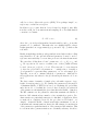
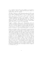
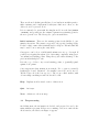
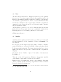
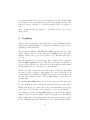
EasySDE User Guide
Oscar Garcı́a
University of Northern British Columbia
[email protected]
July 2003
Contents
1 What
2
2 Theory
3
2.1
Growth, height, and site . . . . . . . . . . . . . . . . . . . . .
3
2.2
Site index . . . . . . . . . . . . . . . . . . . . . . . . . . . . .
4
2.3
Estimation . . . . . . . . . . . . . . . . . . . . . . . . . . . .
6
2.4
Model selection and hypothesis testing . . . . . . . . . . . . .
9
3 Program usage
9
3.1
Data format . . . . . . . . . . . . . . . . . . . . . . . . . . . .
9
3.2
Model specification . . . . . . . . . . . . . . . . . . . . . . . .
10
3.3
Pre-processing
. . . . . . . . . . . . . . . . . . . . . . . . . .
12
3.4
Run . . . . . . . . . . . . . . . . . . . . . . . . . . . . . . . .
14
3.5
Results . . . . . . . . . . . . . . . . . . . . . . . . . . . . . . .
14
4 Graphing
15
1
1
What
EasySDE is essentially a GUI front-end to some old software for developing
forest height growth (or site index) models. Fairly sophisticated and statistically efficient methods are used, making good use of almost any kind of
remeasurement data. The old software was not particularly user-friendly,
which undoubtedly limited its popularity. EasySDE greatly simplifies the
process. Its ease of use should compare favourably to most other site modelling procedures.
In short, various parameterizations of the Richards equation can be used.
For estimation, environmental and measurement error sources are modelled
through a stochastic differential equation (SDE). All parameters are estimated simultaneously by maximum likelihood (don’t panic, all this will be
explained shortly). Data can be two or more height-age measurements on
any number of sample plots. Measurement intervals can vary, and may be
of any length. Either permanent sample plot or stem analysis data can be
used.
Some methodological background is given in the next section. EasySDE
user instructions follow. This should be more than sufficient for model
development using the variants that past experience has shown to be the
most useful. If you really know what you are doing, and feel adventurous,
for added flexibility you might want to run directly the underlying programs.
Or even hack into the code, or use some of its components for other purposes.
Details are contained in the Advanced and Programmer Notes included in
this distribution. All sources are freely available under the MIT license
(www.opensource.org/licenses).
The models and methods are described formally in Garcı́a (1983), and
Seber and Wild (1989, pp. 354–356 and Appendix C), but what follows
should be enough to get you started. Extensive experimental results are
reported in Garcı́a (1999). Similar methods were used by Rennolls (1995).
2
2
2.1
Theory
Growth, height, and site
On a given site, and under “average” weather conditions, the expected height
growth depends on the current height:
dH
= f (H) ,
dt
(1)
where H is top height and t is time (or age). It is usually assumed that,
within limits, other stand variables such as density do not significantly affect
top height. It might be argued that growth also depends on age. But in fact,
age, as elapsed time since birth, does not have a physical presence at any
given time — other than perhaps in the number of growth rings. Therefore,
it can hardly have a direct causal effect. Only accumulated changes reflected
in the current state of the stand can be causes. In principle, physiological
tissue aging might have some influence on growth rates. For the most part,
however, tree size must be the dominant variable.
Starting from some initial height H0 at time t0 , accumulation (i.e., integration) of the growth rate in (1) produces the height H1 at some other
time t1 . This can be calculated taking advantage of (1) being a “separable
differential equation”:
H1
H0
dH
f (H)
dH
f (H)
=
=
dt
t1
t0
dt = t1 − t0 .
If we can analytically integrate the left-hand side, and then solve for H1 , we
obtain a formula for H1 as a function of t1 , t0 , and H0 .
A flexible and commonly used model has f (H) = ηH m − κH. It was proposed in this form by von Bertalanffy in the 1930’s, not just with m = 2/3 as
is often thought (von Bertalanffy, 1938, 1949), and was popularized for plant
growth by Richards (1959). Introduced in forestry by Pienaar and Turnbull
(1973), for some reason it is sometimes called the “Chapman-Richards”
3
model. It will be convenient to use a power transformation H c , with
c = 1 − m, and write it as
dH c
= b(ac − H c ) .
dt
(2)
The equivalence can be verified by differentiating on the left-hand side, and
re-arranging. Integrating and solving for H, as explained above, gives the
height-over-age equation:
H = a[1 − (1 − H0c /ac )e−b(t−t0 ) ]1/c .
(3)
I have omitted the subscript 1 to simplify. We shall also refer to t as age,
although it only needs to be a relative time or nominal age; shifting by a
constant does not make any difference.
In (3), often H0 and t0 are taken as zero, forcing the curve to go through the
origin. More generally, they may represent some initial size at a certain age.
This is a typical sigmoid curve. The parameter a is the asymptote, b is a
“speed” factor, scaling the time axis, and c is a shape parameter determining
the relative height of the inflection point.
2.2
Site index
Top height growth is widely used as an indicator of site productivity. The
advantage over more direct measures, such as volume production, is that it
is less affected by stand density management treatments. It is assumed that
height-age curves, e.g. (3), vary across sites. Depending on site quality, the
curves lie at different levels, without intersecting each other. The curves
may be labeled in various ways, a common one being by the height reached
at some specified reference or base age: the site index.
Mathematically, this corresponds to a one-parameter family of curves. That
is, the curve equations for different sites differ only in the value of one scalar
parameter. For instance, in (2) and (3) one of the parameters a, b, or c, may
change with site quality, while the others are common to all sites. More
generally, this may happen after a re-parameterization: any or all of a, b
and c can be fixed functions of some other parameter that varies with site.
4
We call a site-dependent parameter local, being specific to a sample plot,
and the others global, pertaining to the model as a whole.
The relationship between the local parameter and the conventional site index
S is found by substituting the base age ts in (3):
S = a[1 − (1 − H0c /ac )e−b(ts −t0 ) ]1/c .
(4)
In simpler cases (4) can be algebraically solved for the local parameter, and
this substituted in (3) to obtain a height-age equation indexed by S. A
numerical solution may be needed in other instances.
All this is fairly straightforward in a deterministic world, or when dealing
with “expected” trends as up to here. With actual stand data we need to be
more precise. Implicit in the traditional concept seems to be the idea that
site curves and site index represent some sort of average over hypothetical
stands that might grow in the site. That is, site index is a property of the
site. More recently, some researchers have been thinking of site index as
the actual height reached by a specific stand at the base age. A property
of the stand. Failing to distinguish between these two different definitions,
which we might dub “site site-index” and “stand site-index”, has caused
a great deal of confusion and unnecessary controversy (see, for instance,
Bailey and Cieszewski, 2000, and references therein).
We take the site site-index view. Specifically, Site index is the most likely
top height at a base age among any hypothetical stands (of a given species,
etc.) that could grow in a site 1 . And similarly for other ages.
At least in this view, the site index base age is essentially arbitrary, a device for assigning a number to each curve in the family. Therefore, modelling approaches where results change with the chosen reference age are,
at best, ugly. Our methods are strictly base-age invariant, in the sense of
Bailey and Clutter (1974).
Warning: As with any single-number measure, the concept of site index
can fail if pushed too far. It can be a good indicator of relative productivity
within biogeoclimatic regions where growth patterns and limiting factors are
similar. Otherwise, not just the level, but also curve shape may vary in such
1
I could have said “expected” instead of “most likely”. Mean and mode converge to
the same value as sample size increases, so, presuming an infinite number of hypothetical stands, it makes no difference in the definition. There are differences in estimation
situations, as discussed later.
5
a way that crossings occur. An appropriate stratification should be used.
Alternatively, multidimensional indicators might be possible, although little
or no research in this direction appears to have been done. An experimental
model variant with two local parameters is included in this package.
2.3
Estimation
Rational parameter estimation requires some sort of model for the variability
of the observations. Experience suggests that moderate deviations from
the assumptions — e.g., additive errors, uniform variance, independence,
normality, etc. in regression — may not be overly critical for the quality of
the estimates. A rough characterization of the error structure is nevertheless
desirable.
It is clear, for instance, that the deviations of a stand from the model of
equation (3) would tend to increase with time, and that they are not statistically independent. This because the “error”, due among other things
to weather fluctuations, accumulates over time. Ordinary least-squares is
therefore relatively inefficient. Seber and Wild (1989, Ch. 7) review approaches to modelling this kind of data, and others are found in the forestry
literature. Many, such as autoregressive and mixed effects models, trade a
somewhat crude representation of error structure for the convenience of using standard statistical packages. We try a more realistic stochastic model
that requires special-purpose software. Hopefully, EasySDE now makes its
application not more difficult than other methods.
For each sample plot, we represent the effects of “environmental noise”,
mostly weather, as a perturbation added to the right-hand side of (2). The
perturbation is assumed to be a continuous random process, with values that
are independent for non-overlapping intervals. Technically, what is called a
Wiener, white noise, or Brownian motion process:
√
dH c
= b(ac − H c ) + 2bσ ẇ(t) .
dt
(5)
Here ẇ(t) is the standard (mean 0, variance 1) Wiener process, and σ is a
new parameter determining the perturbation intensity or variance2 . This is
√
The factor 2b does not appear in Garcı́a (1983). If I remember correctly, it was
introduced here to simplify the programming, or maybe for some other obscure reason.
2
6
called a stochastic differential equation (SDE). To keep things “simple”, we
neglect any correlations across plots.
In addition, we recognize that an observed stand top height hi may differ
from the real Hi due to measurement and sampling error. For mathematical
convenience we assume
hci = Hic + σm i ,
(6)
where the i are independent standard normal variables, and σm is another
parameter to be estimated. This makes the error slightly higher for larger
heights (standard error approximately proportional to Hi1−c ), which seems
reasonable.
Finally, it might happen that growth perturbations are higher at the seedling
stage than later on. An optional additional parameter σ0 may be used to
represent extra variability over some time previous to the first measurement.
The general model has then 8 “basic” parameters: a, b, c, t0 , H0 , σ, σm , and
σ0 . In a specific model version or variant, some of these parameters may
be fixed (often zero), global, or local. They may also be some function
of other new global and local parameters — examples later. Actually, a
“local parameter” represents many parameters, one for each sample plot.
Typically, one needs to estimate hundreds of parameters. Although for
most applications only values for the globals among the first five above are
used.
The data consists of a number of sample plots, each with a sequence of ageheight observation pairs (ti , hi ). We estimate the parameters by the method
of maximum likelihood (ML). It in based on calculating the probability,
under the model, of obtaining the observed data. Considered as a function
of the parameters, substituting the given data, this is the likelihood function.
The ML estimates are the parameter values that maximize the likelihood
function. ML estimation has a number of nice statistical properties. Two
characteristics are particularly attractive for this kind of application. First,
no matter how complicated a model, the procedure is well defined: one
“simply” obtains the likelihood function and finds a maximum. Second, it
is invariant under transformations, that is, the ML estimate for any function
of the parameters equals that function of the parameter ML estimates. This
is convenient where parameterizations are essentially arbitrary: should we
7
get good estimates for the site index, for its logarithm, for a local parameter,
for the height at a certain age? Unlike with other methods, all these are
simultaneously possible and compatible.
The likelihood function is obtained through integrating the SDE (5), and
incorporating the distributions implied by (6). If you must, see Garcı́a
(1983) or Seber and Wild (1989) for the gory details. A modified full Newton
method, using first and second derivatives, is used to improve efficiency and
reliability in minimizing the negative of the log-likelihood over hundreds
of variables (parameters). The implementation makes use of the special
structure of the problem, with partitioning strategies to take advantage of
sparsity in the matrix of second derivatives. For details see Garcı́a (1980),
and the Advanced and Programmer Notes in this package.
It might be worthwhile to clarify a couple of things that have caused some
confusion. I probably shot myself in the foot by delving in the Biometrics
paper in theoretically interesting but practically less important limitations
of the model. Some have misunderstood this and dismissed the whole approach as useless, so let us try to keep things in perspective. No model is
perfect, nor it should be: perfection has an unacceptable cost in terms of
parsimony and estimation efficiency. The first quibble was mentioning that
(5) cannot be strictly correct; the additive random perturbation could conceivably make the (transformed) height to go negative. True, but in reality
unlikely and inconsequential. The same thing is routinely ignored without
a second thought when using regressions with non-negative variables. The
second issue may be a little more troubling, at least from a methodological point of view: Often, although not always, the estimate of either σ or
σm turns out to be zero. Apparently the data does not provide sufficient
information to separate the different variance components. Of course, the
problem would go away if either one of the two sources of variability is ignored, as has been done in all the other methods I know off. At any rate,
this does not seem to have an appreciable impact on the estimates for the
parameters of interest (a, b, c, t0 ), and might be taken as a warning against
the temptation of introducing even more “realistic” error structures. Actually, measurement/sampling error in stem analysis is small relative to that
in sample plots (although the risk of bias is higher), and there it might not
be a bad idea to fix σm = 0.
8
2.4
Model selection and hypothesis testing
Models with the same number of parameters can be compared and chosen
according to the highest value of the computed likelihood, or of its logarithm,
the log-likelihood. In comparing models with different number of parameters, extra flexibility needs to be penalized. Various theories suggest adding
penalties of one-half to three log-likelihood units per parameter. Akaike’s
information criterion (AIC), perhaps the most popular, prescribes one unit.
Note that the likelihood value by itself is essentially meaningless, it is the
relative values, or differences in the logarithms, that are important.
For hypothesis testing, one approach considers a log-likelihood difference of
about two units as “significant”. More orthodox is a likelihood-ratio test. It
is based on the fact that twice the log-likelihood difference is asymptotically
distributed as a χ2 with degrees-of-freedom equal to the difference in number
of parameters. For examples see Garcı́a (1999).
3
3.1
Program usage
Data format
The data must be arranged in a text file with three columns: plot number,
age, and top height. Plot numbers must be integers, with up to 9 digits.
The other values are free format, and columns may be separated by any
number of spaces and/or tabs.
Each row corresponds to one measurement date, with the sequence of plot
measurements ordered by increasing age. Different plots must be separated
by a blank line. See test.dat for an example.
Before going any further, it is a good idea to plot the data to check for
“funnies”. SitePlot may be used for this. A detailed description is in Section
4, but for plotting just data it should be self-explanatory.
A note on stem analysis data. Often heights are interpolated for every
year, using methods such as those described by Dyer and Bailey (1987).
Only values for the actual crosscuts should be used here. Because in general
the tree tip corresponding to the ring count at a crosscut is located some
9
distance above the crosscut, crosscut heights may be adjusted as shown by
Dyer and Bailey (1987). However, as suggested by Jim Goudie (BC Ministry
of Forests, quoted by Nigh (1995)), a simpler and probably better method
is to use the crosscut height, reducing the ring count by 0.5 years.
3.2
Model specification
On running EasySDE, the window in Figure 1 appears. The items in it are
as follows:
Figure 1: Stage 1: Model specification window
Title. One line of optional descriptive information to be printed at the
top of the program output.
10
Binary files. If checked, the data and local parameter estimates from the
last run are used. The model version in the new run must use the same local
parameter(s).
File.
Name of the input data file.
Scaling. The ages and heights in the data file are divided by these values.
Convergence is usually faster and more reliable if the scaled ages and heights
are not too far from unity. If the scale factors are different from one, the
initial estimates and the output correspond to the scaled model. Values such
as 10 or 100 make easy the scaling back.
Model. Click to select a model version. The Gi stand for global parameters, and the Li for local parameters. A number of models are available in
EasySDE:
ALOCAL has a as local parameter, and is forced to pass through the origin.
It produces anamorphic site index curves. A-T0 to A-T0S0 include non-zero
origin parameters, and/or the additional initial variance σ0 . ALOCBH is for
data using breast-height age; it forces a height of 1.3 at age zero (before
scaling).
BLOCAL to BLOCBH are similar, but taking b as the local parameter. The
resulting curves are “polymorphic”. Actually, proportional along the t axis.
LINEAR and COMP are more general models, where curve shape varies in a
more flexible way with site. At the cost of an extra parameter. Unfortunately, only a numerical solution for the local as a function of site is possible,
so they are not as convenient for many uses3 . They can be useful for assessing the adequacy of the simpler models, and as a last resort if the others do
not work. COMP was used in Garcı́a (1996).
Finally, ABLOCALS has both a and b as local parameters, so it does not
produce traditional site index curves. It may be useful for hypothesis testing
and experimentation. Graphing the relationship between the estimated a
and b might suggest appropriate re-parameterizations.
3
Conjecture: there are no “truly” polymorphic models with a base-age invariant explicit expression for the indexing parameter in terms of site index.
11
These are the models that generally have been found most useful in practice.
Other variants can be implemented with just a little more effort; see the
Advanced and Programmer Notes.
It is recommended to start with the simplest model in each class (ALOCAL
or BLOCAL), and possibly use the estimated parameters as starting point for
the more general ones. The Binary files option is useful there.
Initial estimates. These are the starting points for the likelihood optimization iterations. They must correspond to the specified scaling, if any.
For the local(s), a same value is initially used for all plots. Tab and Shift-Tab
may be used to move among the entry fields.
Convergence can be slow or fail if initial estimates are not good enough. If
possibly, try stepping through models of increasing complexity, using previous estimates as starting points. Using Binary files takes advantage of the
previous individual-plot locals.
It is also a good idea to try several starting points, to (partially) guard
against local optima.
Some suggestions when starting from scratch: For a, guess a reasonable
height upper bound. Parameter c lies usually between 0.5 and 1; try 0.7.
Try the reciprocal of the base age for b. The σ’s are a little trickier; with
decent scaling something around 0.05 should be OK.
Help.
Displays an abbreviated version of this section.
Quit.
As it says.
Next. Advances to the next stage.
3.3
Pre-processing
On clicking Next, the information is checked, and prepared for use by the
main estimation program. If there are no missing or incorrect entries in the
Model window, the window in Figure 2 appears.
12
Figure 2: Stage 2: Data pre-processing window.
No user input is required. The input data file is checked for consistent plot
numbers and increasing ages. If there are no error messages, the number of
plots is displayed, and we can go to the next stage by clicking Next. The
contents of the message window can be saved to a file through the Save
button.
If you must know, the front-end runs DataPrep.exe, which reads the input
data file and generates intermediate files with the data (DATA.$$$, binary),
the locals (PARS.$$$, binary), and other info (CTRL.$$$, text). If everything
goes well, these are then passed on to SDEfit.exe, which does the hard work.
The final local estimates and other information are left in PARS.$$$, and
results in REPORT.$$$ (a text file). There is a little more flexibility when
running these programs manually, specifically, a list of plot-specific local
initial estimates can be used; see the advanced notes.
13
3.4
Run
The same window is then used to display the iteration log as the optimization proceeds. To monitor progress, values for the parameters and for the
function being minimized (which is -2 times the log-likelihood) are shown for
each iteration, together with some other more esoteric information. Most
relevant, the contribution to the objective function and the local parameter
estimates for a few plots are shown, followed by iteration number, function,
and global parameter values.
The run should be possible to be aborted by clicking the Quit button (but it
isn’t!). Otherwise, the program runs for up to a maximum of 200 iterations.
If this happens try a better starting point and/or better scaling.
Clicking Next takes us to:
3.5
Results
A similar window displays the final results report. The report starts with
the run identification, and the termination condition: “CONVERGED” for a
successful run.
For each plot, the following is shown: Plot number. Number of measurements. Contribution to -2 times the log-likelihood (large values flag outliers).
Local parameter(s) estimate(s). Their approximate standard error. An estimated site index for each plot can be obtained from the local parameter
using (4).
General info follows: Number of plots. Total number of measurements.
Log-likelihood.
Then, info on the global parameters: Estimates. Approximate standard
errors. Matrix of approximate correlations between them4 .
Finally, for the local parameter(s): Average of the estimates. Mean standard error. Mean correlations among local parameters. Mean correlations
between local and global parameters.
4
As mentioned at the end of Section 2.3, often one of the variance estimates turns out
to be zero. Take with a pinch of salt.
14
Note that all results involve the specified scaling factors, if any. Back scaling
can be figured-out by substituting in (5) the age and height divided by the
respective factors. Can also be obtained from the SitePlot program, see
below.
Before exiting, the user is prompted to optionally save the report, if not
already saved.
4
Graphing
SitePlot aids in plotting the data and site index curves. Running SitePlot
brings up the window in Figure 3. It generates commands for gnuplot, a free
graphing program (included).
The first part is similar to EasySDE. The Title appears at the top of the
graph. Only models 1 to 12 are supported. Scaling factors and scaled
parameter values can be used. It is possibly to plot just data, just curves,
or both.
Once the parameters are given, the site index equation can be displayed
with the Show equation button. This gives top height as a function of
age, site index, and index age (Section 2.2). It is in gnuplot format, which
is fairly standard except for using ** for exponentiation.
On the lower part of the window, labels and ranges for the Age and Height
axes can be given or changed. Any strings can be used for the labels. If
a range limit is left blank it is calculated by gnuplot automatically from
the data and/or function values. The age limits must be given when not
plotting data.
For plotting site index curves one needs the index age, the range from
lowest to highest site index, and the site index interval between the curves.
Finally, we may choose to draw a grid or not, and different line types for the
curves can be selected (enter test in gnuplot to see the types available).
If everything goes well, on clicking OK gnuplot is executed, and the graph is
displayed. The user is left in gnuplot, where the graph can be embellished,
printed (right-click on the graph window), saved in various formats, etc. Enter set terminal and help terminal to see the output formats available.
15
Figure 3: Graphing with SitePlot.
For instance, entering set output ’filename.eps’, followed by set term
post eps 20 and replot, produces a good quality Encapsulated PostScript
file.
Gnuplot is an excellent general-purpose graphing program, well worth
learning. See www.gnuplot.info. There is a good brief tutorial at
www.duke.edu/˜hpgavin/gnuplot.html.
The gnuplot commands are left in the file siteplot.plt. This can be loaded
from gnuplot, possibly after manual editing. The gnuplot executable is
Wgnuplot.exe.
16
References
Bailey, R. L., Cieszewski, C. J., 2000. Development of a well-behaved siteindex equation: jack pine in north-central Ontario: Comment. Canadian
Journal of Forest Research 30, 1667–1668.
Bailey, R. L., Clutter, J. L., 1974. Base-age invariant polymorphic site
curves. Forest Science 20, 155–159.
Dyer, M. E., Bailey, R. L., 1987. A test of six methods for estimating true
heights from stem analysis data. Forest Science 33, 3–13.
Garcı́a, O., 1980. A stochastic differential equation model for the height
growth of forest stands. Presented at the 5th Australian Statistical Conference, Sydney. http://web.unbc.ca/˜garcia/unpub/oz80.pdf.
Garcı́a, O., 1983. A stochastic differential equation model for the height
growth of forest stands. Biometrics 39, 1059–1072.
Garcı́a, O., 1996. Toward new site index curves for Douglas-fir in the Netherlands. Working paper, Royal Veterinary and Agricultural University, Unit
of Forestry. http://web.unbc.ca/˜garcia/unpub/dfsite.pdf.
Garcı́a, O., 1999. Height growth of Pinus radiata in New Zealand. New
Zealand Journal of Forestry Science 29 (1), 131–145.
Nigh, G. D., 1995. Compatibility improvements and bias reduction in heightage models. Research Report 03, British Columbia Ministry of Forests,
Research Branch.
Pienaar, L. V., Turnbull, K. J., 1973. The Chapman-Richards generalization
of von Bertalanffy’s growth model for basal area growth and yield in evenaged stands. Forest Science 19, 2–22.
Rennolls, K., 1995. Forest height growth modelling. Forest Ecology and
Management 71 (3), 217–225.
Richards, F. J., 1959. A flexible growth function for empirical use. Journal
of Experimental Botany 10, 290–300.
Seber, G. A. F., Wild, C. J., 1989. Nonlinear Regression. Wiley.
von Bertalanffy, L., 1938. A quantitative theory of organic growth (Inquiries
on growth laws. II). Human Biology 10, 181–213.
von Bertalanffy, L., 1949. Problems of organic growth. Nature 163, 156–158.
17