1
Errata
Title & Document Type: 16500A/16501A Logic Analysis System User's Guide
Manual Part Number: 16500-97007
Revision Date: February 1994
HP References in this Manual
This manual may contain references to HP or Hewlett-Packard. Please note that HewlettPackard's former test and measurement, semiconductor products and chemical analysis
businesses are now part of Agilent Technologies. We have made no changes to this
manual copy. The HP XXXX referred to in this document is now the Agilent XXXX.
For example, model number HP8648A is now model number Agilent 8648A.
About this Manual
We’ve added this manual to the Agilent website in an effort to help you support your
product. This manual provides the best information we could find. It may be incomplete
or contain dated information, and the scan quality may not be ideal. If we find a better
copy in the future, we will add it to the Agilent website.
Support for Your Product
Agilent no longer sells or supports this product. You will find any other available
product information on the Agilent Test & Measurement website:
www.tm.agilent.com
Search for the model number of this product, and the resulting product page will guide
you to any available information. Our service centers may be able to perform calibration
if no repair parts are needed, but no other support from Agilent is available.
User’s Guide
Publication number 16500-97007
First Edition, February 1994
For Safety information, Warranties, and Regulatory
information, see the pages behind the index
© Copyright Hewlett-Packard Company 1987, 1990, 1993, 1994
All Rights Reserved
HP 16500B /16501A Logic
Analysis System
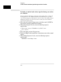
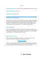
HP 16500B—At a Glance
A system of measurement modules
The HP 16500B is the mainframe of the
Hewlett-Packard Logic Analysis System.
It offers a modular structure for plug-in
cards with a wide range of state, timing,
oscilloscope, and pattern generator
capabilities.
ii
A powerful, easy-to-use interface
The touchscreen interface offers popup menus and color graphics to lead
you through measurement
configurations without having to
remember lots of steps. You can add a
keyboard or mouse to speed data input
and measurement configuration.
The HP 16501A expands module
capacity
The HP 16501A is the add-on mainframe
for expanding the module capacity of
the HP 16500B. When the two are
connected, they form a single ten-card
system that is turned on and controlled
by the HP 16500B.
Intermodule measusurement capability
The HP 16500B offers intermodule
measurement features that allow you to
capture complex system activity.
Modules can
• be armed by an external instrument,
• be armed by another module in the
HP16500B or HP16501A frames, or
• be used to arm an external
instrument.
iii
Install measurement modules in any
slot
Single card analyzers, oscilloscopes,
and other options can go in any slot of
the HP 16500B or HP 16501A. You should
generally begin installing cards starting
with the bottom-most slot and working
up.
Some measurement modules have
multiple cards. A multiple-card module
must be installed into adjacent slots in
the same mainframe—that is, you
cannot install one card of the module
into the HP 16500B and the other into
the HP 16501A.
iv
Calibrate measurement modules after
installation
Some measurement modules are
sensitive to temperature and voltage
variations between different
mainframes. Thus, when you install
such a module in the mainframe, you
should calibrate it before using it to
ensure maximum measurement
precision and accuracy.
See the Service Guide for each
measurement module for installation
and calibration procedures.
In This Book
This User’s Guide shows you how to use
the HP 16500B Logic Analysis System in
your everyday debugging work.
Chapter 1, “Triggering,” shows you how to
set up the analyzer to trigger on the
various kinds of events present in your
system. Advanced triggering capability
allows you to look at only the program
states of interest when you are solving a
particular problem.
Chapter 2, “Intermodule Measurements,”
shows you how to configure multiple
HP 16500 modules and external
measurement instruments into a single
measurement system in which modules
trigger each other.
1
Triggering
2
Intermodule Measurements
3
File Management
4
Concepts
5
Solving Problems
6
Application Notes
Glossary
Index
Chapter 3, “File Management,” shows you
how to transfer files to and from the
HP 16500B using flexible disks, LAN
interfaces, and other interfaces.
Chapter 4,“Concepts,” gives you a brief
introduction to the ideas underlying the
trigger sequencer and the inverse
assembler, two important components of
sophisticated logic analysis.
Chapter 5, “Solving Problems,” shows you
how to diagnose and correct the more
common types of problems that might
occur while you are making a
measurement.
Chapter 6, “Application Notes,” lists the
various application notes that HP has
published regarding the HP 16500B and
other similar HP logic analyzers. These
v
notes will give you more information about specific application problems and
how to solve them using an HP logic analyzer.
See Also
For general information on setup and operation of the HP 16500B, see the
HP 16500B /16501A Logic Analysis System User’s Reference.
For information on programming the HP 16500B using a computer controller
such as a workstation or personal computer, see the HP 16500B/16501A
Logic Analysis System Programmer’s Guide.
For information on logic analyzers, oscilloscopes, preprocessors, and other
logic analysis system options, see the User’s Reference manual for those
options.
vi
Contents
1 Triggering
To store and time the execution of a subroutine 1–3
To trigger on the nth iteration of a loop 1–5
To trigger on the nth recursive call of a recursive function 1–7
To trigger on entry to a function 1–9
To capture a trace of activity associated with a write of known bad data to a
particular variable 1–11
To trigger on a loop that occasionally runs too long 1–12
To verify that all stacks and registers are restored correctly before exiting a
subroutine 1–13
To trigger after all status bus lines finish transitioning 1–15
To find the nth occurrence of asserting a chip select line 1–16
To verify that the chip select line of a memory chip is strobed after the address on the address bus is stable 1–17
To trigger when expected data does not appear on the data bus from a remote device when requested 1–18
To test minimum and maximum pulse limits 1–20
To detect a handshake violation 1–22
To detect bus contention 1–23
Cross-Arming Trigger Examples
1–24
To examine software execution when a timing violation occurs 1–25
To look at control and status signals during execution of a routine 1–26
2 Intermodule Measurements
Intermodule Measurement Examples
2–4
To set up a group run of modules within the HP 16500B 2–5
To start a group run of modules from an external trigger source 2–7
To start an external instrument on command from a module within the HP
16500 and 16501 mainframe 2–9
To see the status of a module within an intermodule measurement 2–11
o see time correlation of each module within an intermodule measurement
2–12
To use a timing analyzer to detect a glitch 2–13
vii
Contents
To capture the waveform of a glitch 2–14
o capture state flow showing how your target system processes an interrupt
2–15
Using stimulus-response to test a cir cuit 2–17
To use a state analyzer to trigger timing analysis of a count-down on a set of
data lines 2–19
To use two state analyzers to monitor the activity of coprocessors in a target
system 2–20
Special displays 2–21
To interleave trace lists 2–22
To view trace lists and waveforms together on the same display 2–24
Skew Adjustment 2–26
To adjust for minimum skew between two modules involved in an intermodule measurement 2–27
3 File Management
Transferring Files Using the Flexible Disk Drive
3–3
To save a measurement configuration 3–4
To load a measurement configuration 3–6
To save a trace list in ASCII format 3–8
To save a menu or measurement as a graphic image 3–10
To load system software 3–12
Using the HP 16500L LAN Interface 3–13
To set up the HP 16500B 3–14
To transfer data files from the HP 16500B system to your computer 3–16
To transfer graphics files from the HP 16500B system to your computer
3–18
4 Concepts
The Trigger Sequencer
viii
4–3
Contents
The Inverse Assembler
4–10
Configuration Translation for Analyzer Modules
4–13
5 If You Have a Problem
Analyzer Problems
5–3
Intermittent data errors 5–3
Unwanted triggers 5–3
No Setup/Hold field on format screen 5–4
No activity on activity indicators 5–4
Capacitive loading 5–4
No trace list display 5–5
Preprocessor Problems 5–6
Target system will not boot up 5–6
Slow clock 5–7
Erratic trace measurements 5–7
Inverse Assembler Problems
5–9
No inverse assembly or incorrect inverse assembly
Inverse assembler will not load or run 5–10
5–9
Intermodule Measurement Problems 5–11
An event wasn't captured by one of the modules 5–11
Messages
5–12
“Default Calibration Factors Loaded” (HP 16540, 16541, and 16542)
“. . . Inverse Assembler Not Found” 5–12
“Measurement Initialization Error” 5–13
“No Configuration File Loaded” 5–14
“Selected File is Incompatible” 5–14
“Slow or Missing Clock” 5–14
“State Clock Violates Overdrive Specification” 5–15
“Time from Arm Greater Than 41.93 ms” 5–15
5–12
ix
Contents
“Waiting for Trigger” 5–15
6 Application Notes
x
1
Triggering
Triggering
As you begin to understand a problem in your system, you may realize
that certain conditions must occur before the problem occurs. You can
use sequential triggering to ensure that those conditions have
occurred before the analyzer recognizes its trigger and captures
information.
You set up sequential triggering as follows:
• Select the Trigger menu for the module you are using.
• In the Trigger menu, define terms and associated values to be used
when searching through the sequence.
• In the Trigger menu, select the number of the state sequence level
you want to modify, and enter the appropriate store qualification,
sequence-advance specification, and sequence-Else specification.
If you aren’t familiar with the trigger menus, try working through the
examples in the Logic Analyzer Training Kit manual, or refer to the
User’s Reference for your analyzer.
12
Triggering
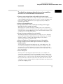
To store and time the execution of a subroutine
To store and time the execution of a subroutine
Most systems software of any kind is composed of a hierarchy of functions
and procedures. During integration, testing, and performance evaluation, you
will want to look at specific procedures to verify that they are executing
correctly and that the implementation is efficient. The analyzer allows you to
do this by triggering on entry to the address range of the subroutine and
counting the elapsed time since the trigger state.
1 Select the state analyzer Trigger menu.
2 Set Count to Time.
Setting the Count to Time causes the state analyzer to store a time stamp for
each data point that is stored in trace memory. The trace list will show these
time stamps next to each state.
3 Define a range term, such as Range1, to represent the address range
of the subroutine of interest.
You may need to examine the structure of your code to help determine this. If
your subroutine calls are really procedure calls, then there is likely to be
some code at the beginning of the routine that adjusts the stack for local
variable allocation. This will precede the address of the first statement in the
procedure. If your subroutine has no local storage and is called by a jump or
branch, then the first statement will also be the entry address.
4 Under State Sequence Levels, enter the following sequence
specification:
• While storing “no state” Trigger on “In_range1” 1 time
• While storing “In_range1” Then find “Out_range1” 1 time
• Store “no state”
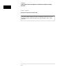
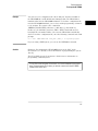
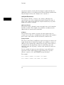
Example
Suppose you want to trigger on entry to a routine called MY_SUB. You can
define the address of MY_SUB in the Format menu, allowing you to reference
the symbol name when setting up the trace specification. Assume that
MY_SUB extends for 0A hex locations. You can set up the trigger sequencer
as shown in the display.
13
Triggering
To store and time the execution of a subroutine
Trigger Setup for Storing Execution of a Subroutine
For processors that do prefetching of instructions or have pipelined
architectures, you may want to add part or all of the depth of the pipeline to the
start address for In_Range1 to ensure that the analyzer does not trigger on a
prefetched but unexecuted state.
14
Triggering
To trigger on the nth iteration of a loop
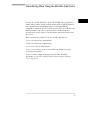
To trigger on the nth iteration of a loop
Traditional debugging requires print statements around the area of interest.
This is not possible in most embedded systems designs. But, the analyzer
allows you to view the system’s behavior when a particular event occurs.
Suppose that your system behaves incorrectly on the last iteration of a loop,
which, in this instance, happens to be the 10th iteration. You can use the
analyzer’s triggering capabilities to capture that iteration and subsequent
processor activity.
1 Select the state analyzer Trigger menu.
2 Define the terms LP_START and LP_END to represent the start and
end addresses of statements in the loop, and LP_EXIT to represent
the first statement executed after the loop terminates.
3 Under State Sequence Levels, enter the following sequence
specification:
• While storing “no state” Find LP_END 1 time
• While storing “anystate” TRIGGER on LP_START 9 times; Else on
“LP_EXIT” go to level 1
• Store “anystate”
The above sequence specification has some advantages and a potential
problem. The advantages are that a pipelined processor won't trigger until it
has executed the loop 10 times. Requiring LP_END to be seen at least once
first ensures that the processor actually entered the loop; then, 9 more
iterations of LP_START is really the 10th iteration of the loop. Also, no
trigger occurs if the loop executes less than 10 times: the analyzer sees
LP_EXIT and restarts the trigger sequence. The potential problem is that
LP_EXIT may be too near LP_END and thus appear on the bus during a
prefetch. The analyzer will constantly restart the sequence and will never
trigger. The solution to this problem depends on the structure of your code.
You may need to experiment with different trigger sequences to find one that
captures only the data you wish to view.
15
Triggering
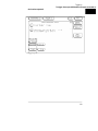
To trigger on the nth iteration of a loop
Trigger Setup for Triggering on the 10th Iteration of a Loop
16
Triggering
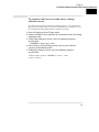
To trigger on the nth recursive call of a recursive function
To trigger on the nth recursive call of a recursive
function
1 Select the state analyzer Trigger menu.
2 Define the terms CALL_ADD, F_START, and F_END to represent the
called address of the recursive function, and the start and end
addresses of the function. Define F_EXIT to represent the address of
the first program statement executed after the original recursive call
has terminated.
Typically, CALL_ADD is the address of the code that sets up the activation
record on the stack, F_START is the address of the first statement in the
function, and F_END is the address of the last instruction of the function,
which does not necessarily correspond to the address of the last statement. If
the start of the function and the address called by recursive calls are the
same, or you are not interested in the function initialization code, you can use
F_START for both CALL_ADD and F_START.
3 Under State Sequence Levels, enter the following sequence
specification:
• While storing “no state” Find “F_END” 1 time
• While storing “anystate” Then find “F_START” 1 time
• While storing “anystate” TRIGGER on “CALL_ADD” 20 times Else on
“F_EXIT” go to level 1
• Store “anystate”
As with the trigger specification for “To trigger on the nth iteration of a loop,”
this specification helps avoid potential problems on pipelined processors by
requiring that the processor already be in the first recursive call before
advancing the sequencer. Depending on the exact code used for the calls, you
may need to experiment with different trigger sequences to find one that
captures only the data you wish to view.
17
Triggering
To trigger on the nth recursive call of a recursive function
Triggering on the 22nd Call of a Recursive Function
18
Triggering
To trigger on entry to a function
To trigger on entry to a function
This sequence triggers on entry to a function only when it is called by one
particular function.
1 Select the state analyzer Trigger menu.
2 Define the terms F1_START and F1_END to represent the start and
end addresses of the calling function. Define F2_START to represent
the start address of the called function.
3 Under State Sequence Levels, enter the following sequence
specification:
• While storing “anystate” Find “F1_START” 1 time
• While storing “anystate” TRIGGER on “F2_START” 1 time Else on
“F1_END” go to level 1
• Store “anystate”
This sequence specification assumes there is some conditional logic in
function F1 that chooses whether or not to call function F2. Thus, if F1 ends
without the analyzer having seen F2, the sequence restarts.
The specification also stores all execution inside function F1, whether or not
F2 was called. If you are interested only in the execution of F1, without the
code that led to its invocation, you can change the storage specification from
“anystate” to “nostate” for the second sequence term.
19
Triggering
To trigger on entry to a function
Triggering on Entry to a Function
110
Triggering
To capture a trace of activity associated with a write of know
particular variable
To capture a trace of activity associated with a write
of known bad data to a particular variable
The trigger specification ANDs the bad data on the data bus, write
transaction on the status bus, and address of the variable on the address bus.
1 Select the state analyzer Trigger menu.
2 Define the terms BAD_DATA, WRITE, and VAR_ADDR to represent
the bad data value, write status, and the address of the variable.
3 Under State Sequence Levels, enter the following sequence
specification:
• While storing “anystate” TRIGGER on “BAD_DATA • WRITE •
VAR_ADDR” one time (you use the Combination trigger term to do this)
• Store “anystate”
Capturing a Bad Write to a Variable
111
Triggering
To trigger on a loop that occasionally runs too long
To trigger on a loop that occasionally runs too long
This example assumes the loop normally executes in 14 µs.
1 Select the state analyzer Trigger menu.
2 Define terms LP_START, LP_END, and Timer1 to represent the start
and end addresses of the loop, and the normal duration of the loop.
You can make the sequence specification closer to the problem domain by
renaming Timer1 to LOOP_DUR.
3 Under State Sequence Levels, enter the following sequence
specification:
• While storing “anystate” Find “LP_START” 1 time
• While storing “anystate” TRIGGER on “LOOP_DUR 14.00 µs” 1 time Else
on “LP_END” go to level 1
You will need to start the LOOP_DUR timer (Timer1) upon entering
this state. You do this using the Timer Control field in the menu for
sequence level 2.
• Store “anystate”
112
Triggering
To verify that all stacks and registers are restored correctly be
subroutine
Triggering on a Loop Overrun
To verify that all stacks and registers are restored
correctly before exiting a subroutine
The exit code for a function will often contain instructions for deallocating
stack storage for local variables and restoring registers that were saved
during the function call. Some language implementations vary on these
points, with the calling function doing some of this work, so you may need to
adapt the procedure to suit your system.
1 Select the state analyzer Trigger menu.
2 Define terms SR_START and SR_END to represent the start and end
addresses of the subroutine.
3 Under State Sequence Levels, enter the following sequence
specification:
• While storing “anystate” Find “SR_START” 1 time
• While storing “anystate” Then find “SR_END” 1 time
• While storing “anystate” TRIGGER on “≠ SR_START” 1 time Else on
“SR_START” go to level 2
113
Triggering
To verify that all stacks and registers are restored correctly before exiting a
subroutine
• Store “anystate”
Verifying Correct Return from a Function Call
Only three sequence terms are shown on the display at a time. You can scroll
through the terms using the knob when the “State Sequence Levels” field is
light blue.
114
Triggering
To trigger after all status bus lines finish transitioning
To trigger after all status bus lines finish transitioning
In some applications, you will want to trigger a measurement when a
particular pattern has become stable. For example, you might want to trigger
the analyzer when a microprocessor’s status bus has become stable during
the bus cycle.
1 Select the timing analyzer Trigger menu and define a term called
PATTERN to represent the value to be found on the label
representing the status bus lines.
2 Under Timing Sequence Levels, enter the following sequence
specification:
TRIGGER on “PATTERN” > 40 ns
115
Triggering
To find the nth occurrence of asserting a chip select line
To find the nth occurrence of asserting a chip select
line
1 Select the timing analyzer Trigger menu.
2 Define the glitch/edge1 term to represent the asserting transition on
the chip select line.
You can rename the Edge1 term to make it correspond more closely to the
problem domain, for example, to CHIP_SEL.
3 Under Timing Sequence Levels, enter the following sequence
specification:
TRIGGER on “CHIP_SEL” 10 times
Triggering on the 10th Assertion of a Chip Select Line
116
Triggering
To verify that the chip select line of a memory chip is strob
on the address bus is stable
To verify that the chip select line of a memory chip is
strobed after the address on the address bus is stable
1 Select the timing analyzer Trigger menu.
2 Define a term called ADDRESS to represent the address in question
and the Edge1 term to represent the asserting transition on the chip
select line.
You can rename the Edge1 term to suit the problem, for example, to
MEM_SEL.
3 Under Timing Sequence Levels, enter the following sequence
specification:
• Find “ADDRESS” > 80 ns
• TRIGGER on “MEM_SEL” 1 time Else on “≠ ADDRESS” go to level 1
Verifying Setup Time for Memory Address
117
Triggering
To trigger when expected data does not appear on the data bus from a remote
device when requested
To trigger when expected data does not appear on the
data bus from a remote device when requested
1 Select the timing analyzer Trigger menu.
2 Define a term called DATA to represent the expected data, the Edge1
term to represent the chip select line of the remote device, and the
Timer1 term to identify the time limit for receiving expected data.
You can rename the Edge1 and Timer1 terms to match the problem domain,
for example, to REM_SEL and ACK_TIME.
3 Under Timing Sequence Levels, enter the following sequence
specification:
• Find “REM_SEL” 1 time
• TRIGGER on “ACK_TIME > 16.00 µs” 1 time Else on “DATA” go to level 1
You will need to use the Timer Control field in the sequence setup for
sequence level 2 to start the ACK_TIME timer upon entering that sequence
level.
This sequence specification causes the analyzer to trigger when the data does
not occur in 16 µs or less. If it does occur within 16 µs, the sequence restarts.
Specifications of this type are useful in finding intermittent problems. You
can set up and run the trace, then cycle the system through temperature and
voltage variations, using automatic equipment if necessary. The failure will be
captured and saved for later review.
118
Triggering
To trigger when expected data does not appear on the data b
device when requested
Triggering When I/O Data Not Returned
119
Triggering
To test minimum and maximum pulse limits
To test minimum and maximum pulse limits
1 Select the timing analyzer Trigger menu.
2 Define the Edge1 term to represent the positive-going transition, and
define the Edge2 term to represent the negative-going transition on
the line with the pulse to be tested.
You can rename these terms to POS_EDGE and NEG_EDGE.
3 Define the Timer1 term to represent the minimum pulse width, and
the Timer2 term to represent the maximum pulse width.
You can rename these terms to MIN_WID and MAX_WID. In this example,
Timer1 was set to 496 ns and Timer2 was set to 1 µs. Both timers start when
sequence level 2 is active.
4 Under Timing Sequence Levels, enter the following sequence
specification:
• Find “POS_EDGE” 1 time
• Then find “NEG_EDGE” 1 time
• TRIGGER on “MIN_WID 496 ns + MAX_WID 1.00 µs” 1 time Else on
“anystate” go to level 1
Because both timers start when entering sequence level 2, they start as soon
as the positive edge of the pulse occurs. Once the negative edge occurs, the
sequencer transitions to level 3. If at that point, the MIN_WID timer is less
than 496 ns or the MAX_WID timer is greater than 1 µs, the pulse width has
been violated and the analyzer should trigger. Otherwise, the sequence is
restarted.
Measurement of Minimum and Maximum Pulse Width Limits
120
Triggering
To test minimum and maximum pulse limits
Triggering when a Pulse Exceeds Minimum or Maximum Limits
121
Triggering
To detect a handshake violation
To detect a handshake violation
1 Select the timing analyzer Trigger menu.
2 Define the Edge1 term to represent either transition on the first
handshake line, and the Edge2 term to represent either transition on
the second handshake line.
You can rename these terms to match your problem, for example, to REQ and
ACK.
3 Under Timing Sequence Levels, enter the following sequence
specification:
• Find “REQ” 1 time
• TRIGGER on “REQ” 1 time Else on “ACK” go to level 1
Triggering on a Handshake Violation
122
Triggering
To detect bus contention
To detect bus contention
In this sequencer setup, the trigger occurs only if both devices assert their
bus transfer acknowledge lines at the same time.
1 Select the timing analyzer Trigger menu.
2 Define the Edge1 term to represent assertion of the bus transfer
acknowledge line of one device, and Edge2 term to represent
assertion of the bus transfer acknowledge line of the other device.
You can rename these to BTACK1 and BTACK2.
3 Under Timing Sequence Levels, enter the following sequence
specification:
TRIGGER on “BTACK1 • BTACK2” 1 time
Triggering on Bus Contention
123
Cross-Arming Trigger Examples
The following examples use cross arming to coordinate measurements
between two instruments. The cross-arming is set up in the Arming
Control menu (obtained by selecting Arming Control in the Trigger
menu). When coordinating measurements between two or more
analyzers, select Count Time so you can correlate the measurements
made by the two analyzers.
See Also
Chapter 2, “Intermodule Measurements.”
124
Triggering
To examine software execution when a timing violation occu
To examine software execution when a timing
violation occurs
The timing analyzer triggers when the timing violation occurs, and when it
triggers, it also sets its “arm” level to true. When the state analyzer receives
the arm signal, it triggers immediately on the present state.
1 Select the timing analyzer Trigger menu.
2 Define the Edge1 term to represent the control line where the timing
violation occurs.
3 Under Timing Sequence Levels, enter the following sequence
specification:
TRIGGER on “glitch/edge1” 1 time
4 Select the state analyzer Trigger menu and accept the default
(anystate) definition for term a.
5 Under State Sequence Levels, enter the following sequence
specification:
• While storing “anystate” TRIGGER on “arm • a” 1 time
• Store “anystate”
125
Triggering
To look at control and status signals during execution of a routine
To look at control and status signals during execution
of a routine
The state analyzer will trigger on the start of the routine whose control and
status signals are to be examined with finer resolution than once per bus
cycle. When it triggers, it will switch its “arm” level true. The timing analyzer
will trigger when it receives the true arm level and detects the transition
represented by glitch/edge1.
1 Select the state analyzer Trigger menu and define term R_START to
represent the starting address of the routine.
2 Under State Sequence Levels, enter the following sequence
specification:
• While storing “anystate” TRIGGER on “R_START” 1 time
• Store “anystate”
3 Select the timing analyzer Trigger menu.
4 Define the Edge1 term to represent a transition on one of the control
signals.
5 Under Timing Sequence Levels, enter the following sequence
specification:
TRIGGER on “arm • Edge1” 1 time
126
2
Intermodule Measurements
Intermodule Measurements
An intermodule measurement is a measurement that is coordinated
between two or more modules to capture different types of
information related to a problem you are trying to solve. This chapter
shows you how to make several kinds of intermodule measurements.
Intermodule measurements can involve state analyzers, timing
analyzers, oscilloscopes, and pattern generators. The measurement
may be as simple as coordinating the startup of several modules
during a measurement; it may be quite complex and include multiple
arming sequences between modules and external equipment.
For example, you may have a timing analyzer detect the occurrence of
a glitch, and at the same time, have an oscilloscope capture the glitch
waveform and a state analyzer capture the program flow before and
after the occurrence of the glitch. With several types of information
obtained from various analysis modules, you can discover problems
that would otherwise be difficult to identify.
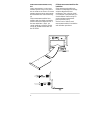
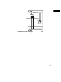
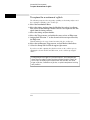
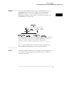
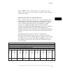
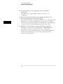
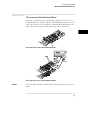
The figure on the opposite page shows how intermodule bus arming
signals are connected between modules inside the HP 16500B and
HP 16501A. Note that any arm input can be driven by any slot, and
that the port input line can drive any slot.
If you are unfamiliar with the basic operation of the Intermodule
Menu, try working the examples in the Logic Analyzer Training Kit.
22
Intermodule Measurements
Intermodule Bus Block Functional Diagram
23
Intermodule Measurement Examples
To set up an intermodule measurement, you must use the Intermodule
menu. All modules that will participate in the intermodule
measurement must be represented in this menu and their
relationships must be shown under the Group Run field.
24
Intermodule Measurements
To set up a group run of modules within the HP 16500B
To set up a group run of modules within the
HP 16500B
Modules are armed in the configuration tree by either an individual module or
the Group Run field. When armed, a module begins searching for the input
that will satisfy its trigger specification. To obtain a specification that triggers
on the arm signal, specify to trigger on “anystate.”
1 Select the Intermodule menu.
2 Select the second field down from the top on the left, then select
Group Run.
3 Select the name of each module you want to include in the
measurement.
The modules are listed under “Modules” on the right side of the menu.
a Select Group Run if you want to arm this module immediately when
the Group Run begins.
b Select the name of another module if you want the other module to
arm the present one when the other module finds its trigger.
c Select Independent if this module should not be included in the
intermodule measurement.
4 Select the Group Run field in the upper right hand corner.
The group run begins. The modules attached directly to the Group Run field
immediately begin searching for their respective trigger conditions. When a
module finds its trigger, it arms any modules attached to it in the Group Run
tree.
25
Intermodule Measurements
To set up a group run of modules within the HP 16500B
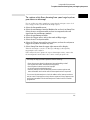
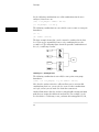
The analyzer in slot
B is armed when
the oscilloscope in
slot D finds its
trigger condition.
Oscilloscope Arms State Analyzer in Group Run
26
Intermodule Measurements
To start a group run of modules from an external trigger sour
To start a group run of modules from an external
trigger source
1 Connect the arm signal from the external instrument or system to the
PORT IN BNC connector on the rear panel of the HP 16500 frame.
2 Select the Intermodule menu.
3 Set up the group run specification.
4 Select the PORT IN/OUT field.
a Select the field under PORT IN Level, then select the level that
matches the external signal that will be applied to the PORT IN BNC
on the HP 16500B rear panel.
The choices are TTL, ECL, and User. The latter allows you to specify a
voltage from −4.00 V to +5.00 V using an onscreen keypad.
b Select the field under PORT IN Edge to change from Rising to Falling
edge and vice-versa for the rear-panel input signal.
c Select Done to leave the PORT IN/OUT Setup menu.
5 Select the Group Run field in the upper right hand corner.
The modules attached directly to the Group Run Armed from PORT IN field
wait for a signal from the PORT IN field.
6 Start the external instrument or system.
When the external instrument sends the proper signal to the PORT IN BNC,
the internal modules attached directly to the Group Run Armed from PORT
IN field are armed and begin searching for their respective trigger conditions.
Modules are armed by modules above them, either an individual module or the
field named Group Run Armed from PORT IN. That is, in the intermodule display,
an arrow pointing to a module to be armed originates in the module providing
the arm signal. See the figure “Oscilloscope Arms State Analyzer in Group Run”
on page 2-6. When armed, a module begins searching for the input that will
satisfy its trigger specification. To obtain a specification of “trigger on the arm
signal,” specify a trigger that equates to “trigger on anything.”
See Also
“To set up a group run of modules within the HP 16500B.”
27
Intermodule Measurements
To start a group run of modules from an external trigger source
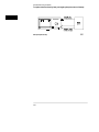
Both the analyzer
in slot B and the
oscilloscope in
slot D are armed
when the PORT IN
signal arrives.
State Analyzer and Oscilloscope armed from PORT IN
See Also
“To set up a group run of modules within the HP 16500B” in this chapter.
28
Intermodule Measurements
To start an external instrument on command from a mod
HP 16500 and 16501 mainframe
To start an external instrument on command from a
module within the HP 16500 and 16501 mainframe
You can set up a module in a group run so that it sends a pulse through the
PORT OUT rear panel BNC. The pulse can be used to start or stop a
measurement in an external instrument or system.
1 Set up the group run specification.
See “To start a group run of modules within the HP 16500B” or “To start a
group run of modules from an external trigger source.”
2 Select PORT IN/OUT.
The PORT IN/OUT Setup menu appears.
3 Select the PORT OUT field.
• Select Off if no module should drive PORT OUT.
or
• Select the name of the module you want to have drive PORT OUT.
4 Select Done in the PORT IN/OUT Setup menu.
The output from the PORT OUT BNC is an active high TTL level.
See Also
“To set up a group run of modules within the HP 16500B” or “To start a group
run of modules from an external trigger source” in this chapter.
29
Intermodule Measurements
To start an external instrument on command from a module within the HP 16500
and 16501 mainframe
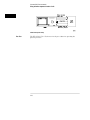
The analyzer in
slot B drives port
out after finding its
trigger.
Driving the Port Out BNC in an Intermodule Measurement
210
Intermodule Measurements
To see the status of a module within an intermodule measure
To see the status of a module within an intermodule
measurement
1 Select the Intermodule menu.
2 Find the name of the module under the “Modules” list, and read the
status under the module name.
The status can be either Running or Stopped. You can interpret these
indications as follows:
• If a module was running and is now stopped, assume it received its arming
signal, triggered, and finished its measurement properly.
• If a module located below a stopped module on the intermodule
configuration tree has received an arming signal and is still running, either
it is still waiting to satisfy its trigger specification or it has not captured
enough information to fill its memory.
• If a module below a running module on the intermodule configuration tree
has not received its arming signal, it will not begin running until the upper
module finds its trigger condition.
Both modules are
running because
neither has found
its respective
trigger condition.
Module Status
211
Intermodule Measurements
To see time correlation of each module within an intermodule measurement
To see time correlation of each module within an
intermodule measurement
Time correlation in the intermodule menu can help you see when the trigger
occurred for each module and the relative time range of data captured by
that module.
1 Select Time in the Count field of the trigger menu of each logic state
analyzer whose measurement will be time-correlated with the other
modules.
Timing analyzers and digitizing oscilloscopes implicitly count time because
their sampling is driven by an internal clock, rather than an external state
clock. See the User’s Reference for your logic state analyzer for details on
how to count time with the analyzer.
2 Select the Intermodule menu.
3 Select the Group Run field in the upper right hand corner.
Once the measurement has started, view the time correlation bars at the
bottom of the Intermodule Menu. The “T” in each bar indicates the relative
time at which that module found its trigger condition. The yellow portion of
each bar indicates the start and stop points of the acquisition window of the
associated module relative to the other modules in the measurement.
This portion of the bar
indicates the relative
time range of data
acquired by this
module.
T indicates the time at
which the trigger was
found.
212
Intermodule Measurements
To use a timing analyzer to detect a glitch
To use a timing analyzer to detect a glitch
The following setup uses a state analyzer to capture state flow occurring at
the time of the glitch. This can be useful in troubleshooting. For example, you
might find that the glitch is ground bounce caused by a number of
simultaneous signal transitions.
1 Select the Intermodule menu.
2 Select the timing analyzer from the Modules list and set it to Group
Run. Select the state analyzer and set it to respond to the arm signal
from the timing analyzer.
You must have fully independent state and timing analyzers to make this type
of measurement. For example, though the HP 16550A can be configured to
use some of its channels for a state analyzer and some for a timing analyzer, it
cannot present those analyzers independently for intermodule
measurements.
3 Select the timing analyzer Trigger menu.
4 Select an Edge term. Then assign glitch detection “*” to the channels
of interest represented by the Edge term.
5 Select the state analyzer Trigger menu.
6 Set the analyzer to trigger on any state and store any state.
7 Select Group Run in the upper right corner of the display.
If you don’t see the activity of interest in the state trace, try changing the
trigger position using the Acquisition Control field in the Trigger menu of the
state analyzer. By changing the Acquisition mode to manual, you can position
the trigger at any state relative to analyzer memory.
The timing analyzer can detect glitch activity on a waveform. A glitch is defined
as two or more transitions across the logic threshold between adjacent timing
analyzer samples.
213
Intermodule Measurements
To capture the waveform of a glitch
To capture the waveform of a glitch
The following setup uses the triggering capability of the timing analyzer and
the acquisition capability of the oscilloscope.
1 Select the Intermodule Menu.
2 Select the timing analyzer from the Modules list and set it to Group
Run. Select the oscilloscope module and set it to respond to the arm
signal from the timing analyzer.
3 Select the timing analyzer module.
4 Select the Trigger menu, and within the menu, select an Edge term.
5 Assign glitch detection “*” to the channel of interest represented by
the Edge term.
This will usually be the same channel monitored by the oscilloscope.
6 Select the oscilloscope Trigger menu, and set Mode to Immediate.
7 Select the Group Run field in the upper right corner.
If you have trouble capturing the glitch waveform on the oscilloscope, try
adjusting the skew in the Intermodule menu, so the oscilloscope triggers
earlier.
A timing analyzer can trigger on a glitch and capture it, but a timing analyzer
doesn’t have the voltage or timing resolution to display the glitch in detail. An
oscilloscope can display a glitch waveform with fine resolution, but cannot
trigger on glitches, combinations of glitches, or sophisticated patterns involving
many channels.
214
Intermodule Measurements
To capture state flow showing how your target system proces
To capture state flow showing how your target system
processes an interrupt
Use an oscilloscope with a sample rate faster than the microprocessor clock
rate to trigger on the asynchronous interrupt request.
1 Select the Intermodule menu.
2 Select the oscilloscope from the Modules list and set it to Group Run.
3
4
5
6
7
Select the state analyzer module and set it to respond to the arm
signal from the oscilloscope module.
Select the oscilloscope module.
Select the Trigger menu, and set the mode to Edge trigger.
Select the state analyzer module.
Select the Trigger menu of the state analyzer, and set the analyzer to
trigger on any state and store any state.
Select Group Run from the upper right corner of the display.
When the interrupt occurs, the oscilloscope will trigger, subsequently
triggering the state analyzer.
If the analyzer doesn’t capture the expected interrupt activity, ensure that
the interrupt isn’t masked due to the actions of other program code.
This setup can help you answer questions like the following:
•
•
•
•
•
Does the processor branch to the proper interrupt handling routine?
Are registers and status information saved properly?
How long does it take to service the interrupt?
Is the interrupt acknowledged properly?
After the interrupt is serviced, does the processor restore registers and
status information and continue with the interrupted routine as expected?
You can use the state analyzer to check the address of the interrupt routine as
well as to see if interrupt processing is done as expected. Using a preprocessor
and inverse assembler with the state analyzer will make it easier to read the
program flow.
215
Intermodule Measurements
To capture state flow showing how your target system processes an interrupt
Interrupt Capture Setup
216
Intermodule Measurements
Using stimulus-response to test a circuit
Using stimulus-response to test a circuit
1 Select the Intermodule menu.
2 Select the pattern generator from the Modules list and set it to Group
Run. Select the oscilloscope module and set it to respond to the arm
signal from the pattern generator. Select the state analyzer and set it
to respond to the arm signal from the pattern generator.
3 Load the pattern generator with the proper patterns to simulate the
signals from the driving hardware.
4 Insert the “Signal IMB” instruction at the desired point in the pattern
generator program.
The arm signal is programmable. It can occur anywhere in the pattern
generator cycle.
5 Select the oscilloscope Trigger Menu. Set the oscilloscope to trigger
on signals of interest in the circuit under test.
6 Select the state analyzer Trigger Menu. Set the analyzer to trigger on
addresses, data, or status conditions of interest, and to store any state
or states of interest.
7 Select Group Run from the upper right corner of the display.
The pattern generator will begin its cycle, and will arm the oscilloscope and
state analyzer.
In the early stages of system design and integration, you may want to test a
circuit when the driving hardware that will stimulate it has not yet been
designed or fabricated. You can also use the pattern generators with the logic
analyzer to test PC boards when no board-test system is available.
The HP 16520A and HP 16521A pattern generators for the HP 16500B avoid the
inconvenience of having to stack several signal generators on top of each
other, with all of the cable connections required for those signal generators.
Additionally, you have a single interface to access all the test modules in your
measurement.
217
Intermodule Measurements
Using stimulus-response to test a circuit
Stimulus-Response Setup
See Also
The HP 16520A User’s Reference for the procedures for operating the
pattern generator.
218
Intermodule Measurements
To use a state analyzer to trigger timing analysis of a count-d
data lines
To use a state analyzer to trigger timing analysis of a
count-down on a set of data lines
1 Select the Intermodule menu.
2 Select the state analyzer from the Modules list and set it to Group
Run. Select the timing analyzer and set it to respond to the arm signal
from the state analyzer.
3 Select the state analyzer Trigger menu.
4 Set the state analyzer to trigger on the label and term that identify the
start of the count-down routine.
If you are not familiar with the procedures for setting up a trigger condition,
see chapter 1.
5 In the timing analyzer Trigger Menu, set the timing analyzer to trigger
on any state and store any state.
6 Select Group Run from the upper right corner of the display.
Your target system may include various state machines that are started by
system events: interrupt processing, I/O activity, and the like. The state analyzer
is ideal for recognizing the system events; the timing analyzer is ideal for
examining the step-by-step operation of the state machines.
219
Intermodule Measurements
To use two state analyzers to monitor the activity of coprocessors in a target
system
To use two state analyzers to monitor the activity of
coprocessors in a target system
1 Select the Intermodule menu.
2 Select the first state analyzer from the Modules list and set it to
Group Run. Select the second state analyzer and set it to respond to
the arm signal from the first analyzer.
3 Select the Trigger menu of the first analyzer.
4 Set the first analyzer to trigger on the problem condition.
Some problems may involve complex sequences of conditions. See chapter 1,
“Triggering,” for more information on defining a trigger sequence.
5 Select the Trigger menu of the second analyzer.
6 Set the second analyzer to trigger on any state and store any state.
7 Select Group Run from the upper right corner of the display.
After the measurement is complete, you can interleave the trace lists of both
state analyzers to see the activity executed by both coprocessors during
related clock cycles.
You can use a similar procedure if you have only one processor, but wish to
monitor its activity with that of other system nodes, such as chip-select lines,
I/O activity, or behavior of a watchdog timer. In some instances it may be
easier to look at related activity with a timing analyzer.
See Also
“Special Displays” in this chapter.
“To use a state analyzer to trigger timing analysis of a count-down on a set of
data lines” in this chapter.
Debugging coprocessor systems can be a complex task. Replicated systems
and contention for shared resources increase the potential problems. Using
two state analyzers with preprocessors can make it much easier to discover
the source of such problems. For example, you may wish to set up one analyzer
to trigger only when a certain problem occurs, and set up the other analyzer to
be armed by the first analyzer so that it takes its trace only when the first
analyzer recognizes its trigger. This will let you observe the behavior of both
coprocessors during the occurrence of a problem.
220
Special displays
Interleaved Trace Lists
Interleaved trace lists allow you to view data captured by two or more
analyzers in a single trace list. When you interleave the traces, you see
each state that was captured by each analyzer. These states are shown
on consecutive lines.
You can interleave state listings from HP 16510B, 16540A, 16540D,
and 16550A state analyzers, when two or more are used together in a
group run. Interleaved state listings are useful when you are using
multiple analyzers to look at interaction between two or more
processors. They are also useful when you need more analysis width
than is available in one analyzer.
Mixed Display Mode
The Mixed Display mode allows you to show state listings and
waveforms together on screen, if all were obtained by modules within
the HP 16500B and 16501A frame. State listings are shown at the top
of the screen and waveform displays are shown at the bottom. You can
interleave state listings from two analyzers at the top of the screen, if
desired. You can display waveforms from two oscilloscopes or timing
analyzers at the bottom of the screen.
221
Intermodule Measurements
To interleave trace lists
To interleave trace lists
1 Set up the analyzers whose data you wish to interleave as part of a
group run.
You won’t need to do this if the two measurement modules for which you
want mixed display are really part of the same module. For example, you
might have an HP 16550A state/timing analyzer configured as two separate
analyzers, one a state analyzer, the other a timing analyzer. You can use
mixed display to view the timing analyzer waveform with the trace lists from
the state analyzer.
2 Select the first state analyzer whose trace list will be shown in the
interleaved display.
3 Select Trigger from the menu field and set Count to Time.
The system uses the time stamps stored with each state to determine the
ordering of states shown in an interleaved trace list.
4 Repeat steps 2 and 3 for the second state analyzer.
5 Select Listing Display from the Menu field.
6 Select one of the label fields in the trace list display, then select
Interleave.
7 Select the name of the analyzer whose trace list will be interleaved
with the first analyzer. Then choose the label that you want to
interleave from the selected analyzer.
Interleaved data is displayed in yellow. Trace list line numbers of interleaved
data are indented. The labels identifying the interleaved data are shown
above the labels for the current analyzer, and are displayed in yellow.
If you have problems with the procedure, and you are using two independent
analyzers, first ensure that the analyzers are set up as part of a group run.
Ensure that each analyzer is set to Count Time and that each analyzer has an
independent clock from the target system.
You can interleave trace lists from state analyzers that were configured as part
of a group run or from state analyzers that are configured as separate analyzers
within the same measurement module. In the first case, you might have two
HP 16550A analyzers configured in a group run; in the second, you might have a
single HP 16550A configured as two state analyzers. The interleaved trace lists
are shown as a time-correlated, state-to-state display.
222
Intermodule Measurements
To interleave trace lists
Labels for the
interleaved states are
shown above those for
the primary analyzer.
Interleaved states are
shown in yellow with
line numbers indented
from those of the
primary analyzer.
Interleaved Trace Lists on the HP 16550A
See Also
“To set up a group run of modules within the HP 16500B” in this chapter.
223
Intermodule Measurements
To view trace lists and waveforms together on the same display
To view trace lists and waveforms together on the
same display
1 Set up the modules whose data you wish to view as part of a group
run.
You won’t need to do this if the two measurement modules for which you
want mixed display are really part of the same module. For example, you
might have an HP 16550A state/timing analyzer configured as two separate
analyzers, one a state analyzer, the other a timing analyzer. You can use
mixed display to view the timing analyzer waveform with the trace lists from
the state analyzer.
2 Select the module for which you wish to show waveforms.
This might be an oscilloscope module or a timing analyzer.
3 Select the label field to the left of the waveform display area twice,
then choose the waveforms to be shown.
When you double-select the label field to the left of the waveform display
area, a new menu appears that allows you to insert and delete signals and
choose the relative display size and position for the signals.
4 Select the state analyzer.
5 Set the Trigger menu of the state analyzer and set the Count field to
Time.
Timing analyzers and digitizing oscilloscopes implicitly count time because
their sampling is driven by an internal clock, rather than an external state
clock. See the manual for your logic state analyzer for details on how to count
time with the analyzer.
6 To insert state listings, select any label field from the state listing.
From the popup that appears, select the desired label to insert.
7 Select Mixed Display from the menu field.
8 Select Group Run from the upper right corner of the display.
You can position X and O Time markers on the waveform display, if desired.
Once set, the time markers will be displayed in both the listing and the
waveform display areas. Note that even if you set X and O Time markers in
another display, you must also set the Time markers in the Mixed Display if
Time markers are desired.
224
Intermodule Measurements
To view trace lists and waveforms together on the same
You can use the Mixed Display feature in the state analyzer menus to show
both waveforms and trace lists in the same display, making it easier to correlate
the events of interest.
If you are using mixed display as part of a group run, you may need to adjust
intermodule skew to ensure proper time correlation and display results.
Mixed Display using the HP 16550A and HP 16532A
See Also
X and O markers from
the waveform display
are shown in their
relative position on the
state display.
“To set up a group run of modules within the HP 16500B” in this chapter.
“Skew Adjustment” in this chapter.
225
Skew Adjustment
You can modify the skew or timing deviation between modules within
the intermodule measurement. This allows you to compensate for any
known delay of the system under test, or to compare two signals by
first removing any displayed skew between the signal channels.
Skew adjustments can correct module delays to within 2 ns of other
modules. Note that the module or channel that is used as the trigger is
normally the reference channel, and adjustments are normally made to
deskew the nonreference channels.
226
Intermodule Measurements
To adjust for minimum skew between two modules involve
measurement
To adjust for minimum skew between two modules
involved in an intermodule measurement
1 Connect an input signal from each module to the same signal.
An ideal signal for testing skew is a single-shot signal with fast risetime. Such
a signal simplifies triggering and makes it easier to correlate the input event
between the modules. Ensure that you use proper probe grounding for
maximum signal fidelity.
2 Select the Intermodule menu.
3 Set up both modules so they will begin searching for the trigger
immediately when a group run begins.
This setup focuses mostly on trying to eliminate probe skew and internal
triggering delays. You can use other intermodule setups as well. For example,
you may be interested in nullifying the effects of the internal arming delay in
a setup where one module arms another.
4 Set up the trigger conditions for each module.
This will depend upon your input signal. For example, if you are adjusting
intermodule skew using a single-shot pulse with a rising edge, set a timing
analyzer to trigger on a rising edge using the Edge1 term, and the
oscilloscope to trigger on a positive slope.
5 Select the Display or Waveform menu in one of the modules.
6 Set up the display so that both input waveforms are displayed
simultaneously.
You do this by selecting the label field to the left of the display twice. The
second selection brings up a new menu that allows you to insert or delete
waveforms. You can delete all but the waveform of interest from the first
module, then add the waveform of interest from the second module. Select
Done when finished.
7 Select Group Run.
You may now need to trigger the signal of interest, if, for example, it is
activated by a push button. You may need multiple events to capture good
waveforms for both measurement modules. Remember that the oscilloscope
captures far more accurate waveform data than the timing analyzer. Thus, if
the waveforms do not match exactly, it may only be because the waveform
edge did not meet the timing analyzer’s setup and hold time specifications for
a particular sampling period.
227
Intermodule Measurements
To adjust for minimum skew between two modules involved in an intermodule
measurement
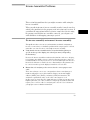
8 Record the difference between waveform events shown by the two
modules.
You can use the X and O markers to measure the differences in delays.
9 Select the Intermodule Menu.
10 Select Skew, then enter a skew correction value for one of the
modules using the knob or the keyboard.
11 Return to the module waveform display and recheck the skew
adjustment.
You will need to repeat steps 7 through 11 as needed until the trigger events
on the two waveforms match as closely as possible.
Before making an intermodule measurement, you should remove skew between
the modules to ensure that a simultaneous arm signal to both modules results in
captures of the same events around the trigger.
Skew Removal Between Timing Analyzer and Oscilloscope
228
3
File Management
File Management
A host computer such as a PC or UNIX workstation can enhance the
HP 16500B in many ways. You can use the host to store configuration
files or measurement results for later review. Screen images from the
HP 16500B can be saved in bitmap files for inclusion in reports
developed using word processors or desktop publishing tools. Or, you
can develop programs on the PC that manipulate measurement results
to satisfy your problem-solving needs.
This chapter shows you some examples of how to transfer files
between a host computer and the HP 16500B, using the flexible disk
drive and the optional HP 16500L LAN Interface. If you aren’t familiar
with basic flexible disk drive operations, see the HP 16500B/16501A
User’s Reference. If you need help setting up or understanding the
use of the HP 16500L LAN Interface, see the HP 16500L LAN
Interface User’s Guide.
You can also use a host computer to send the HP 16500B complex
command sequences—allowing you to automate your measurement
tasks. If you want to program the HP 16500B using a host computer,
see the HP 16500B/16501A Logic Analysis System Programmer’s
Guide and the HP 16500L LAN User’s Guide.
32
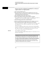
Transferring Files Using the Flexible Disk Drive
Because the flexible disk drive on the HP 16500B will read and write
double-sided, double density or high-density disks in MS-DOS format,
it is a useful tool for transferring images to and from IBM PCcompatible computers as well as other systems that can read and write
MS-DOS format. You can save measurement configuration files,
measurement results, and even menu and measurement images from
the screen.
This section shows you how to use the flexible disk drive to:
• save a measurement configuration
• load a measurement configuration
• save a trace list in ASCII format
• save a screen image (such as an oscilloscope display or menu)
• load system software
If you need more information on the basic flexible disk drive
operations, see the HP 16500B/16501A Logic Analysis System
User’s Reference.
33
File Management
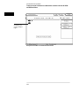
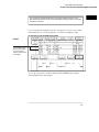
To save a measurement configuration
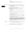
To save a measurement configuration
You can save measurement configurations on a 3.5" disk or on the internal
hard disk for later use. This is especially useful for automating repetitive
measurements for production testing.
1 Select System from the module field.
2 Select Hard Disk or Flexible Disk from the menu field.
3 Select Store from the disk operations field.
4 Select the module for which you want to save the configuration from
the module list.
You can save the configuration for individual modules. The choice “System”
saves only the mainframe configuration. The choice “All” saves the mainframe
configuration and that of all measurement modules.
5 Specify a file name into which to save the configuration using the “to
file” field.
6 Specify a descriptive comment for the file using the “file description”
field.
7 Select Execute.
Saving the Oscilloscope Configuration for Skew Testing
34
File Management
To save a measurement configuration
If you want to save your file in a directory other than the root, you can select
Change Directory from the disk operations field. Then type the name of the
desired directory in the directory name field, or select it from the list of visible
directories using the knob.
35
File Management
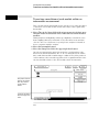
To load a measurement configuration
To load a measurement configuration
You can quickly load a previously saved measurement configuration, saving
the trouble of manually setting up the measurement parameters for each
module.
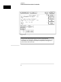
1 Select System from the module field.
2 Select Hard Disk or Flexible Disk from the Menu field.
Your choice here depends on where you saved the configuration.
3 Select Load from the disk operations field.
4 Select the module for which you want to load a configuration from
the module list.
You can load configurations for individual modules. The choice “System”
loads only the mainframe configuration. The choice “All” loads the mainframe
configuration and that of all measurement modules.
However, you can only load configurations that are defined in the
configuration file itself. Thus, if you select System, then select a file that
contains only an analyzer configuration, the configuration will fail.
If you save an analyzer configuration as “All,” then attempt to reload that
configuration into a particular measurement module, configuration will fail.
Also, configurations are slot dependent. If you save a configuration for a
particular module, rearrange the modules within the HP 16500B, then try to
reload the configuration, the configuration will not load.
5 Specify a file name from which to load the configuration using the
“from file” field.
6 Select Execute.
36
File Management
To load a measurement configuration
Loading Configuration for all HP 16500B Modules and the System
37
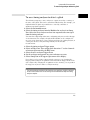
File Management
To save a trace list in ASCII format
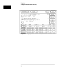
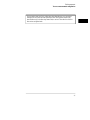
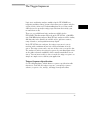
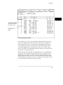
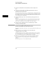
To save a trace list in ASCII format
Some HP 16500B displays, such as file lists and trace lists, contain columns of
ASCII data that you may want to move to a PC for further manipulation or
analysis. You can save these displays as ASCII files, using a procedure similar
to that for creating graphics images. While a graphics capture saves only the
data shown onscreen, saving the display as an ASCII file captures all data in
the list, even if it is offscreen.
1 Insert a DOS-formatted 3.5" disk in the flexible disk drive.
2 Set up the menu you want to capture, or run a measurement from
which you want to save data.
Remember that only displays that present lists of textual data can be
captured as ASCII files.
3 Select Print Disk from the Print menu.
4 Select the Filename field and specify a file name to which the screen
will be printed.
5 Select ASCII (ALL) from the Output Format field.
If the current display contents can’t be saved as an ASCII file, this option will
not be present in the Output Format field.
6 Select Flexible Disk from the Output Disk menu.
7 Select Execute.
38
File Management
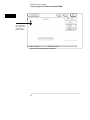
To save a trace list in ASCII format
68332EVS
-
State Listing
Label
ADDR
CPU32 Mnemonic
STAT
__________ _____ ______________________________________ _________________
0
1
2
3
4
5
6
7
8
9
10
11
12
13
14
15
16
17
18
19
20
21
22
406F4
ANDI.L
#********,(A6)+
0FF7A
0004 data write
0FF7C
06F6 data write
40992
BSR.B
0004093E
40994 nu MOVE.B
********,(****,A7)
0FF76
0004 data write
0FF78
0994 data write
4093E
MOVE.W
#03FF,00FFFA46
40940
03FF pgm read
40942
00FF pgm read
40944
FA46 pgm read
40946
MOVE.W
#6B70,00FFFA72
40948
6B70 pgm read
4094A
00FF pgm read
4094C
FA72 pgm read
4094E
RTS
40950 nu MOVE.L
D1,-(A7)
0FF76
0004 data read
0FF78
0994 data read
40994
MOVE.B
00020001,(0004,A7)
40996
0002 pgm read
40998
0001 pgm read
4099A
0004 pgm read
Opcode Fetch
Data Write
Data Write
Opcode Fetch
Opcode Fetch
Data Write
Data Write
Opcode Fetch
Opcode Fetch
Opcode Fetch
Opcode Fetch
Opcode Fetch
Opcode Fetch
Opcode Fetch
Opcode Fetch
Opcode Fetch
Opcode Fetch
Data Read
Data Read
Opcode Fetch
Opcode Fetch
Opcode Fetch
Opcode Fetch
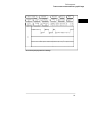
Part of a Trace Listing Saved as an ASCII File
39
File Management
To save a menu or measurement as a graphic image
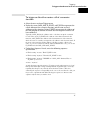
To save a menu or measurement as a graphic image
You can save menus and measurements to disk in one of four different
graphics formats.
1 Insert a DOS-formatted flexible disk in the flexible disk drive.
2 Set up the menu whose image you want to capture, or run a
measurement from which you want to save data.
3 Select Print Disk from the Print menu.
4 Select the Filename field and specify a file name to which the screen
will be printed.
5 Select the Output Format field and specify the output format for the
graphics file.
Choose one of the following formats:
• B/W TIF (SCREEN) is a black and white Tagged Image File Format file in
TIFF version 5.0 format
• Color TIF (SCREEN) is a color TIFF file in TIFF version 5.0 format
• PCX (SCREEN) is a color PCX file (PCX is the PC Paintbrush and
Publisher’s Paintbrush format from ZSoft)
• EPS (SCREEN) is a black and white Encapsulated PostScript file
6 Select Flexible Disk from the Output Disk menu.
7 Select Execute.
310
File Management
To save a menu or measurement as a graphic image
An Oscilloscope Display Saved as a TIF Image
311
File Management
To load system software
To load system software
1 Insert the first disk containing the system software.
2 Select System from the module field.
3 Select Hard Disk from the menu field.
4 Select Change Directory from the disk operation field.
5 Select the directory SYSTEM using the knob, and select Execute.
6 Select Flexible Disk from the menu field.
7 Select Copy from the disk operation field.
8 Select the file you want to update using the knob, then select
Execute.
The selected file is copied to the \SYSTEM directory on the hard disk.
Repeat steps 7 and 8 for all files you need to update. If you have more than
one disk from which you want to copy files, turn the knob after changing
disks. This ensures that the HP 16500B will read the directory on the new
disk.
312
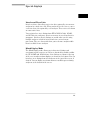
Using the HP 16500L LAN Interface
The HP 16500L LAN Interface option for the HP 16500B extends the
Logic Analysis System by making it look like a NFS (Network File
System) node. Using NFS utilities for the PC or NFS on a UNIX
workstation, you can transfer files to and from the HP 16500B as if it
were a disk drive attached to your machine. The LAN Interface also
creates virtual directories and files for measurement configurations
and measurement results, so you can store and retrieve these as
though they were ordinary files.
This section shows you how to use the HP 16500L to do the following:
• set up the HP 16500B configuration
• retrieve measurement data from a module in the HP 16500B
• transfer images of HP 16500B menu and result screens to your host
computer
If you have not connected your HP 16500B to the network, installed
network software, or learned basic network commands, see the
HP 16500L User’s Guide and the HP 16500L System
Administrator’s Guide before performing the tasks in this chapter.
313
File Management
To set up the HP 16500B
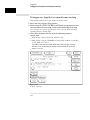
To set up the HP 16500B
You can set up the HP 16500B from the front panel, or via the LAN. To set up
the system via the LAN, you can use one of three methods:
• Copy a configuration file from your PC or workstation to one of the files
called setup.raw in the HP 16500B directory tree.
• Remotely load a configuration file into the system from one of the local
disk drives of the HP 16500B.
• Program the system directly, using the programming commands described
in the HP 16500B System Programmer’s Guide.
Example
You want to load a configuration file called “486_bus” from your local
computer into an HP 16550A state/timing module. The HP 16550A is installed
in slot B of the HP 16500B mainframe. The mainframe is mounted on your
network as disk drive L: (assuming you are using a PC as the host).
To load the configuration file, enter the following at the DOS prompt:
C:\> copy 486_bus L:\slot_b\setup.raw
If you are using a UNIX system, you might use the cp command. In the
Microsoft Windows environment, you can use the File Manager.
314
File Management
To set up the HP 16500B
Example
You want to load a configuration file called “486_bus” from the hard disk of
the HP 16500B into an HP 16550A state/timing module. The HP 16550A is
installed in slot B of the HP 16500B mainframe. To load the configuration file
from the HP 16500B hard disk, you need to send the programming command
to the analyzer. The syntax of the command is:
:MMEMory:LOAD:CONFig <filename>[,<disk drive>][,<slot number>]
In this case, the disk drive parameter, will be “INT0,” which indicates the
hard disk. The slot number will be 2, because the HP 16550A is installed in
slot B. To load the configuration file, enter the following command at the DOS
prompt:
C:\> echo :MEM:LOAD:CON ’486_BUS’,INT0,2
L:\system\program
If you are using a UNIX system, you can use the UNIX echo command.
See Also
Chapter 4, “Programming the HP 16500B System via the LAN,” in the
HP 16500L User’s Guide, for more information on programming the system
directly.
The HP 16500B System Programmer’s Guide for more information on
programming command syntax.
To copy files to the setup.raw file locations, or to send commands to the system
at the \system\program file location, you must be connected to the HP 16500B
system as the control user.
315
File Management
To transfer data files from the HP 16500B system to your computer
To transfer data files from the HP 16500B system to
your computer
You can transfer data from the HP 16500B system to your PC or workstation
by copying files. Data files in binary format are available in file locations
\slot_x\data.raw. These binary files can be transferred to your computer and
then reloaded into the HP 16500B system later.
For some types of measurement modules, data files in ASCII format are also
available. The ASCII data files are in file locations
\slot_x\data.asc\{analyzer name}\{label name}.txt
Depending on which measurement module you are using, there might not be
a subdirectory corresponding to an analyzer name. There is an ASCII data file
corresponding to each label name you have created in the measurement
module.
1 Set up the system for the measurement you want to make.
You can do this from the front panel or remotely.
2 Run the analyzer to acquire data.
You can do this from the front panel or remotely.
3 If you would like the data in binary format, copy the file data.raw to
your computer from the file location \slot_{x}\data.raw
The x represents the slot in which the measurement module is installed.
4 If you would like the data in ASCII format, copy the files
corresponding to the labels you want to view from the file location
\slot_{x}\data.asc\{analyzer name}\{label name}.txt
Depending on which measurement module you are using, there might not be
a subdirectory corresponding to an analyzer name.
See Also
Chapter 3 of the HP 16500L LAN User’s Guide describes the contents of the
binary data.raw file.
316
File Management
To transfer data files from the HP 16500B system to your comp
Example
You have an HP 16550A state/timing analyzer installed in slot C of your
HP 16500B mainframe. The name of analyzer 1 of the HP 16550A is
68000_BUS. You have created some labels under analyzer 1 of the
HP 16550A, including one called “addr_lo.” The directory structure of the
HP 16500B system looks like this:
After setting up a measurement and acquiring data, you want to analyze the
data for label addr_lo on your PC. To copy the ASCII data to your local
computer, enter the following command at the DOS prompt:
C:\ copy L:\slot_c\data.asc\68000_bus\addr_lo {local path
name}
If you are using a UNIX system, you might use the cp command. In the
Microsoft Windows environment, you can use the File Manager.
See Also
“Measurement Module Subdirectories,” in chapter 3 of the HP 16500L LAN
User’s Guide, for more information about the files that are available for
measurement modules.
317
File Management
To transfer graphics files from the HP 16500B system to your computer
To transfer graphics files from the HP 16500B system
to your computer
The current display of the HP 16500B is available in four different formats.
1 Set up the display you want to transfer.
2 Copy the file in the format of your choice from the directory
\system\graphics.
• The file screen.tif is a color Tagged Image File Format file, in TIFF version
5.0 format.
• The file screenbw.tif is a black and white TIFF file in TIFF version 5.0
format.
• The file screen.pcx is a color PCX file. (PCX is the standard format of PC
Paintbrush and Publisher’s Paintbrush.)
• The file screenbw.epi is a black and white Encapsulated PostScript file in
EPS version 3.0 format.
You can also save the current display to a file on one of the local HP 16500B
disk drives, using the Print to Disk function. You can then transfer the file
from the HP 16500B drive to your computer.
These graphics files contain the current display on the HP 16500B screen. The
contents of the files change whenever you change the display. When you copy
one of the graphics files, the display will freeze for a few moments while the
HP 16500B is copying the current display.
Example
To copy a PCX picture of the current screen display to your computer, enter
the following command at the UNIX command prompt:
$ cp /logic/system/graphics/screen.pcx {local path name}
If you are using a DOS system, you can use the copy command. In the
Microsoft Windows environment, you can use the File Manager.
318
4
Concepts
Concepts
Understanding how the analyzer does its job will help you use it more
effectively and minimize measurement problems. This chapter
explains the general operation of the trigger sequencer and the
inverse assembler.
42
The Trigger Sequencer
Logic state and timing analyzer modules for the HP 16500B have
triggering and data storage features that allow you to capture only the
system activity of interest. Understanding how these features work
will help you set up analyzer trigger specifications that satisfy your
measurement needs.
There are several different logic analyzers available for the
HP 16500B. This discussion will focus on the HP 16550A, a 100-MHz
state/500-MHz timing analyzer. Most HP logic analyzers will be similar,
differing only in the number of available states, pattern resources,
range resources, and acquisition memory depth.
In the HP 16550A state analyzer, the trigger sequencer is a state
machine with a minimum of two states and a maximum of twelve
states. The trigger term can be any one of these states except the last.
The analyzer searches for a trigger sequence by matching input values
on the pods to branch conditions, which control transitions between
states. You can insert or delete states to make the trigger sequence as
simple or complex as needed for your application.
Trigger Sequence Specification
See the following figure, which shows a sequence specification with
four states. To define the trigger sequence, you specify sequenceadvance, sequence-else, storage, and trigger-on specifications.
43
Concepts
A sequence-else specification can
branch to the same state...
Sequence-advance
specifications always
branch to the next state.
to a previous state...
or a later state.
Each state can have a
unique storage
specification.
State Analyzer Sequencer with Four States
Each state, except for the last, has two branch conditions. These are
the sequence-advance and sequence-else specification. (The triggeron specification is a special sequence-advance specification that is
described in the section “TRIGGER On Specification.”)
Sequence-Advance Specification
The sequence-advance branch, sometimes called the “if” branch or
primary branch, always branches to the next higher-numbered state.
You can specify the following kinds of sequence-advance
specifications:
Find (or Then find) “<TERM>” <OCCURS> time(S)
Find (or Then find) “<TERM>” <TIME PERIOD>
If the Find (or Then find) “<TERM>” is found <OCCURS> number of
times, the sequencer advances to the next sequence level.
If the <TERM> remains stable for <TIME PERIOD>, the sequencer
advances to the next sequence level.
44
Concepts
Sequence-Else Specification
The sequence-else branch, sometimes called the “else if” branch or
secondary branch, may branch to any other state, including the
current state, a previous state, or a later state. The sequence-else
specification looks like the following:
Else on “<TERM>” go to level <sequence level>
If the Sequence-Else specification is satisfied before the sequenceadvance specification is satisfied, the sequencer begins at <sequence
level>.
The last state may only have a sequence-else branch specification,
which may branch to the same state or a prior state.
Storage Specification
In each state, a storage specification determines the data stored by the
analyzer while it is searching for the sequence-advance, sequenceelse, and trigger specifications. Storage specifications are defined
using the same pattern, range, and timer resources available for
defining branching specifications.
While storing “anystate”, “no state”, or “<TERM>”
Note that if you specify “no state,” the analyzer still stores sequenceadvance terms and TRIGGER terms.
TRIGGER On Specification
If there are branch and storage specifications for each sequence level,
what does the trigger term mean? The trigger term is a special
sequence-advance specification in that, when found, it locks the
contents of analyzer acquisition memory. The trigger can be
positioned at the beginning, middle, or end of acquisition memory.
The trigger specification can look like the following:
TRIGGER on “<TERM>” <OCCURS> times
TRIGGER on “<TERM>” <TIME PERIOD>
If the trigger term is found <OCCURS> times, or if the trigger term
remains stable for <TIME PERIOD>, the trigger is captured in
memory. Then the sequencer advances to the next sequence level. If
45
Concepts
you want to capture activity after the trigger is captured, define an
additional sequence level and specify the desired storage qualification
for post-trigger activity (for example, store “anystate”).
Analyzer Resources
The sequence-advance, sequence-else, storage, and trigger-on
specifications are set by a combination of up to 10 pattern terms, 2
range terms, and 2 timers. Different analyzer models may vary in the
number of resources available.
10 Pattern Terms
The pattern terms, a through j, represent single states to be found on
labeled sets of bits. For example, you could have an address on the
address bits or a status on the status bits.
2 Timers
You can start, stop, continue, or pause the timers upon entry to a
sequence state, then use a comparison of current timer value against a
preset value to determine whether to branch to another state.
2 Range Terms
The range terms, Range1 and Range2, represent ranges of values to be
found on labeled sets of bits. For example, you could have a range of
addresses to be found on the address bus or a range of data values to
be found on the data bus. Range terms are satisfied by any value
within the range for “In_Range,” and any value outside the range for
“Out_Range.”
You can combine the pattern terms and range terms with logical
operators to form complex pattern expressions in the sequenceadvance, sequence-else, and TRIGGER on specifications.
For example,
Find “<TERM1>+<TERM2>” OR <TERM1> and <TERM2>
Find “<TERM1>.<TERM2>” AND <TERM1> and <TERM2>
46
Concepts
Where <TERM> can be a single value on a set of labels, any value
within a range of values on a set of labels, or a glitch or edge transition
on a bit or set of bits.
Limitations Affecting Use of Analyzer Resources
There are limitations on the way resources can be combined to form
complex pattern expressions. Resources are combined in a four-level
hierarchy. First, resources are divided into two groups. The groups
can be combined with AND or OR. Second, within these groups,
resources are combined into pairs. Pairs can also be logically
combined using AND or OR. Third, individual resources are combined
into pairs using AND, NAND, OR, NOR, XOR, NXOR. Fourth,
individual resources may be included or excluded from participating in
a pattern expression. You can also include the logical negation of the
resource.
The following table shows how resources are divided in the
HP 16550A. Remember that some resources may not be available,
depending on the analyzer configuration. For example, if you are using
the analyzer as a state analyzer, the Edge1 and Edge2 resources are
not available. If the timers are off, the Timer1 and Timer2 resources
are not available.
Can combine groups with AND or OR
Group 1
Group 2
Can combine pairs with AND or OR within a group
Pair 1
Pair 2
Pair 3
Pair 4
Pair 1
Combine Resources into pairs using AND, NAND, OR, NOR, NXOR
Include or ExcludeResources
on,
on,
on,
off,
on,
on,
on,
on,
on,
off,
off,
off,
off,
>, <
off,
off,
off,
off,
off,
in
neg
neg
neg
neg
neg
neg
neg
neg
ran
ate
ate
ate
ate
ate
ate
ate
ate
ge,
out
of
ran
ge
a
b
c
Ran
d
Edg
e
Tim
f
g
ge1
e1
er1
Pair 2
on,
off,
neg
ate
h
Pair 3
off,
in
ran
ge,
out
of
ran
ge
Ran
ge2
Pair 4
on,
off,
neg
ate
on,
off,
neg
ate
on,
off,
neg
ate
off,
>, <
i
Edg
e2
j
Tim
er2
47
Concepts
So, the following combinations are valid combinations for the state
analyzer, if timers are on:
(a+b) • (In_Range2 + Timer2 > 400 ns)
(c • Out_Range1) + (f xor g)
The following combinations are not valid, because resources cross pair
boundaries:
(a + c)
(d + Timer1 < 400 ns)
The first example shows that a and c cannot be combined at the first
level. You can get around this, however, by combining them at the
second level. The following figure shows the possible combinations of
the a, b, c and Range1 terms:
Combining a, b, c, and Range1 Terms
The following combination is not valid, because pairs cross group
boundaries:
((a+b) + (h • In_Range2)) • (j xor Timer2 > 400 ns)
Note that the analyzer interface will not allow you to enter invalid
combinations, however, you need to be aware of what combinations
are legal, so that you can make the desired measurement.
Another limitation is that the analyzer cannot handle ranging for input
pods that are assigned to different analysis IC’s. For example, if you
need to define a 32-bit range term, you must do it using pods 1/2, 3/4,
48
Concepts
or 5/6. Trying to define a range across pods 2/3, 4/5, or 1/6 will not
work.
The Timing Analyzer
When you configure the HP 16550A as a timing analyzer, the trigger
sequencer is similar. However, there are between 1 and 10 states
available. The trigger term is always the last state. There are two
additional resources, Edge1 and Edge2. These can recognize
occurrences of a glitch, or occurrences of a rising edge, falling edge,
either edge, or no edge on a bit or ORed set of bits represented by a
glitch/edge term.
49
The Inverse Assembler
When the analyzer captures a trace, it captures binary information.
The analyzer can then present this information in binary, octal,
decimal, hexadecimal, or ASCII. Or, if given information about the
meaning of the data captured, the analyzer can inverse assemble the
trace. The inverse assembler makes the trace list more readable by
presenting the trace results in terms of processor opcodes and data
transactions.
The inverse assembly software needs five pieces of information:
• Address bus. The inverse assembler expects to see the label ADDR,
with bits ordered in a particular sequence.
• Data bus. The inverse assembler expects to see the label DATA,
with bits ordered in a particular sequence.
• Status. The inverse assembler expects to see the label STAT, with
bits ordered in a particular sequence.
• Start state for disassembly. This is the first displayed state in the
trace list, not the cursor position. See the figure below.
• Tables indicating the meaning of particular status and data
combinations.
When you press the Invasm key to begin inverse assembly of a trace,
the inverse assembler begins with the first displayed state in the trace
list. This is called synchronization. It looks at the status bits (STAT)
and determines the type of processor operation, which is then
displayed under the STAT label. If the operation is an opcode fetch,
the inverse assembler uses the information on the data bus to look up
the corresponding opcode in a table, which is displayed under the
DATA label. If the operation is a data transfer, the data and
corresponding operation are displayed under the DATA label. This
continues for all subsequent states in the trace list.
410
Concepts
The inverse assembler
synchronizes at the first
line in the trace list...
not at the cursor
position
Inverse Assembly Synchronization
If you roll the trace list to a new position and press Invasm again, the
inverse assembler repeats the above process. However, it does not
work backward in the trace list from the starting position. This may
cause differences in the trace list above and below the point where
you synchronized inverse assembly. The best way to ensure correct
inverse assembly is to synchronize using the first state you know to be
the first byte of an opcode fetch.
For processors with a pipeline or instruction queue, the information
presented to the analyzer can potentially become confusing. Was an
instruction executed or not? Active circuitry on some preprocessor
models helps by sorting out the order of execution before presenting
information to the analyzer. You can set switches on the preprocessor
to control whether this dequeueing is enabled.
411
Concepts
Symbols
When you specify symbols as the format for displaying the address bus in the
trace list, the symbol lookup happens independently of inverse assembly. Thus,
you can have symbols in the address field without inverse-assembled data and
status. The HP E2450A symbol download utility allows you to download symbols
from OMF (Object Module Format) files.
See Also
The Preprocessor User’s Guide for more information on switch
settings.
Chapter 5, “If You Have a Problem,” if you have problems using the
inverse assembler.
412
Configuration Translation for Analyzer Modules
Configuration files provide an easy way for you to save and restore
measurement setups, simplifying repeated measurements. However,
sometimes you might change analyzer modules in the HP 16500B
Logic Analysis System to gain additional measurement features. Or,
you might want to use a configuration file from one HP 16500B system
on another HP 16500B with a different analyzer module. But, the
analyzer configuration files cannot be transferred directly from one
type of analyzer to the next. Each analyzer has internal architectural
differences, reflected in the number of pods, clock configurations,
trigger sequencer features, analyzer resources, and so on.
To help you move configuration files from one analyzer to another,
some analyzer measurement modules for the HP 16500B Logic
Analysis System support automatic translation of analyzer
configurations. If you save an analyzer configuration from one kind of
analyzer module, then load that configuration into a module that
supports configuration translation, the translator will adjust the
configuration as required to account for differences between the
modules.
The configuration translator needs to account for many aspects of the
analyzer architecture. Some of the considerations are as follows:
• For some analyzers, demultiplexing data will require separate
analyzer pods, because a master clock and a slave clock can’t be
assigned on the same pod to perform the demultiplexing. The
translator may display messages on the analyzer screen that ask you
to reconnect pod cables in a different configuration.
• When a range term is split across multiple pods, the term must span
adjacent odd/even pairs, starting with 1. Thus, terms could span
pods 1 and 2, 3 and 4, 5 and 6, or 7 and 8, but not 2 and 3. Again,
the translator may display messages asking you to reconnect cables
in a different configuration.
• When loading a configuration into an analyzer with fewer pods than
the one on which the configuration was saved, the translator must
413
Concepts
remove pod assignments. Which pods are removed from the
configuration will depend on the widths of each pod in the original
analyzer and new analyzer.
The configuration translation also needs to account for many
differences in the format and trace menus between the analyzers,
including
• label names,
• polarities,
• thresholds,
• symbols,
• clocking,
• number of sequence levels,
• branch conditions, and
• patterns,
among others.
To ensure that trace measurements act as expected when you move
configuration files from one analyzer to another, follow these
recommendations:
• Ensure that the analyzer pods are hooked up as required by the
configuration translation and the new analyzer. The onscreen
messages given by the translator will help you identify which
analyzer pods must be swapped. If you are using an HP
preprocessor, the Preprocessor User’s Guide may contain
information showing the cable connections for different analyzer
modules.
• Review all trace format and trigger menu settings to verify that they
will meet your measurement requirements. You should check label
assignments, channel masks, pattern and range definitions,
sequencer setup, and general analyzer configuration (which pods
are mapped to each analyzer).
414
Concepts
When you move a configuration file from one analyzer to another, the trace
data from previous measurements is not moved. If you need to store trace data
for future reference, see “To save a trace list in ASCII format” in chapter 3.
415
416
5
If You Have a Problem
If You Have a Problem
Occasionally, a measurement may not give the expected results. If you
encounter difficulties while making measurements, use this chapter to
guide you through some possible solutions. Each heading lists a
problem you may encounter, along with some possible solutions. Error
messages which may appear on the logic analyzer are listed below in
quotes “ ”. Symptoms are listed without quotes.
If you still have difficulty using the analyzer after trying the
suggestions in this chapter, please contact your local Hewlett-Packard
service center.
CAUTION
When you are working with the analyzer, be sure to power down both the
analyzer and the target system before disconnecting or connecting cables,
probes, and preprocessors. Otherwise, you may damage circuitry in the
analyzer, preprocessor, or target system.
52
Analyzer Problems
This section lists general problems that you might encounter while
using the analyzer.
Intermittent data errors
This problem is usually caused by poor connections, incorrect signal levels, or
marginal timing.
q
q
q
Remove and reseat all cables and probes; ensure that there are no bent
pins on the preprocessor interface or poor probe connections.
Adjust the threshold level of the data pod to match the logic levels in the
system under test.
Use an oscilloscope to check the signal integrity of the data lines.
Clock signals for the state analyzer must meet particular pulse shape and
timing requirements. Data inputs for the analyzer must meet pulse shape and
setup and hold time requirements.
See Also
See “Capacitive Loading” in this chapter for information on other sources of
intermittent data errors.
Unwanted triggers
Unwanted triggers can be caused by instructions that were fetched but not
executed.
q
Add the prefetch queue or pipeline depth to the trigger address to avoid
this problem.
The depth of the prefetch queue depends on the processor that you are
analyzing. Suppose you are analyzing a pipelined processor having fetch,
decode, execute, and memory stages. The processor fetches 32-bit words. To
ensure that the processor has begun executing a particular routine when the
trigger occurs, set the trigger to the module entry address plus 08 hex. (This
assumes that there is no immediate data in the instruction stream.)
53
If You Have a Problem
No Setup/Hold field on format screen
No Setup/Hold field on format screen
The HP 16540 and 16541 (A and D models), or HP 16542A logic analyzer
cards are not calibrated. Refer to your logic analyzer reference manual for
procedures to calibrate the cards.
No activity on activity indicators
q
q
q
On the HP 16510A Logic Analyzer, check the fuse that allows power to
the preprocessor interface.
On other logic analyzers, check for loose cables, board connections, and
preprocessor interface connections.
Check for bent or damaged pins on the preprocessor probe.
Capacitive loading
Excessive capacitive loading can degrade signals, resulting in incorrect
capture by the preprocessor interface, or system lockup in the
microprocessor. All preprocessor interfaces add additional capacitive loading,
as can custom probe fixtures you design for your application.
Careful layout of your target system can minimize loading problems and
result in better margins for your design. This is especially important for
systems that are running at frequencies greater than 50 MHz.
q
q
See Also
Remove as many pin protectors, extenders, and adapters as possible.
If multiple preprocessor interface solutions are available, try using one
with lower capacitive loading.
Chapter 6 lists some application notes that discuss the problems of probing
high-speed digital systems.
No trace list display
54
If You Have a Problem
No trace list display
If there is no trace list display, it may be that your analysis specification is not
correct for the data you want to capture, or that the trace memory is only
partially filled.
q
q
Check your analysis sequencer specification to ensure that it will
capture the events of interest.
Try stopping the analyzer; if the trace list is partially filled, this should
display the contents of trace memory.
55
Preprocessor Problems
This section lists problems that you might encounter when using a
preprocessor. If the solutions suggested here do not correct the
problem, you may have a defective preprocessor. Refer to the User’s
Guide for your preprocessor for test procedures. Contact your local
Hewlett-Packard Sales Office if you need further assistance.
Target system will not boot up
If the target system will not boot up after connecting the preprocessor
interface, the microprocessor or the preprocessor interface may not be
installed properly, or they may not be making electrical contact.
q
Ensure that you are following the correct power-on sequence for the
preprocessor and target system.
1 Power up the analyzer and preprocessor.
2 Power up the target system.
If you power up the target system before you power up the preprocessor,
interface circuitry in the preprocessor may latch up, preventing proper target
system operation.
q
q
q
q
See Also
Verify that the microprocessor and the preprocessor interface are
properly rotated and aligned, so that the index pin on the
microprocessor (such as pin 1 or A1) matches the index pin on the
preprocessor interface.
Verify that the microprocessor and the preprocessor interface are
securely inserted into their respective sockets.
Verify that the logic analyzer cables are in the proper sockets of the
preprocessor interface and are firmly inserted.
Reduce the number of extender sockets.
“Capacitive Loading” in this chapter.
56
If You Have a Problem
Slow clock
Slow clock
If you have the preprocessor interface hooked up and running and observe a
slow clock or no activity from the interface board, the +5 V supply coming
from the analyzer may not be getting to the interface board.
q
To check the +5 V supply coming from the analyzer, disconnect one of
the logic analyzer cables from the preprocessor and measure across pins
1 and 2 or pins 39 and 40.
• If +5 V is not present, check the internal preprocessor fuse or current
limiting circuit on the logic analyzer. For information on checking this fuse
or circuit, refer to the Service Guide for your logic analyzer.
• If +5 V is present and the cable connection to the preprocessor appears
sound, contact your nearest Hewlett-Packard Sales Office for information
on servicing the board.
Erratic trace measurements
There are several general problems that can cause erratic variations in trace
lists and inverse assembly failures.
q
Ensure that the preprocessor configuration switches are correctly set
for the measurement you are trying to make.
Some preprocessors include configuration switches for various features (for
example, to allow dequeueing of the trace list). See your Preprocessor User’s
Guide for more information.
57
If You Have a Problem
Erratic trace measurements
q
Try doing a full reset of the target system before beginning the
measurement.
Some preprocessor designs require a full reset to ensure correct
configuration.
q
Ensure that your target system meets the timing requirements of the
processor with the preprocessor probe installed.
See “Capacitive Loading” in this chapter. While preprocessor loading is slight,
pin protectors, extenders, and adapters may increase it to unacceptable
levels. If the target system design has poor timing margins, such loading may
cause incorrect processor functioning, giving erratic trace results.
q
Ensure that you have sufficient cooling for the preprocessor probe.
Current processors such as the i486, Pentium™, and MC68040 generate
substantial heat. This is exacerbated by the active circuitry on the
preprocessor board. You should ensure that you have ambient temperature
conditions and airflow that meet or exceed the requirements of the
microprocessor manufacturer.
58
Inverse Assembler Problems
This section lists problems that you might encounter while using the
inverse assembler.
When you obtain incorrect inverse assembly results, it may be unclear
whether the problem is in the preprocessor or in your target system. If
you follow the suggestions in this section to ensure that you are using
the preprocessor and inverse assembler correctly, you can proceed
with confidence in debugging your target system.
No inverse assembly or incorrect inverse assembly
This problem is due to incorrect synchronization, modified configuration,
incorrect connections, or a hardware problem in the target system. A locked
status line can cause incorrect or incomplete inverse assembly.
q
Verify that the inverse assembler has been synchronized by placing an
opcode at the top of the display (not at the input cursor) and pressing
the Invasm key.
Because the inverse assembler works from the first line of the trace display,
if you jump to the middle of a trace and select Invasm, prior trace states are
not disassembled correctly. If you move to several random places in the trace
list and select Invasm each time, the trace disassembly is only guaranteed to
be correct from the top of the display forward for each selection.
q
Ensure that each analyzer pod is connected to the correct preprocessor
cable.
There is not always a one-to-one correspondence between analyzer pod
numbers and preprocessor cable numbers. Preprocessors must supply
address (ADDR), data (DATA), and status (STAT) information to the
analyzer in a predefined order, so the cable connections for each
preprocessor are often altered to support that need. Thus, one preprocessor
might require that you connect cable 2 to analyzer pod 2, while another will
require you to connect cable 5 to analyzer pod 2. See the User’s Guide for
your preprocessor for further information.
59
If You Have a Problem
Inverse assembler will not load or run
q
q
Check the activity indicators for status lines locked in a high or low
state.
Verify that the STAT, DATA, and ADDR format labels have not been
modified from their default values.
These labels must remain as they are configured by the configuration file. Do
not change the names of these labels or the bit assignments within the labels.
Some preprocessors also require other data labels; check your Preprocessor
User’s Guide for more information.
q
Verify that all microprocessor caches and memory managers have been
disabled.
In most cases, if the microprocessor caches and memory managers remain
enabled you should still get inverse assembly, but it may be incorrect since
some of the execution trace was not visible to the logic analyzer.
q
Verify that storage qualification has not excluded storage of all the
needed opcodes and operands.
Inverse assembler will not load or run
You need to ensure that you have the correct system software loaded on your
analyzer.
q
Ensure that the inverse assembler is on the same disk as the
configuration files you are loading.
Configuration files for the state analyzer contain a pointer to the location of
the corresponding inverse assembler. If you delete the inverse assembler or
move it to another location, the configuration process will fail.
q
Make sure you are using the version of the inverse assembler software
that corresponds to the operating system revision installed on your
analyzer.
See your Preprocessor User’s Guide for details.
510
Intermodule Measurement Problems
Some problems occur only when you are trying to make a
measurement involving multiple modules.
An event wasn’t captured by one of the modules
If you are trying to capture an event that occurs very shortly after the event
that arms one of the measurement modules, it may be missed, due to internal
analyzer delays. For example, suppose you set the oscilloscope to trigger
upon receiving a trigger signal from the logic analyzer, because you are trying
to capture a pulse that occurs right after the analyzer’s trigger state. If the
pulse occurs too soon after the analyzer’s trigger state, the oscilloscope will
miss the pulse.
q
Adjust the skew in the Intermodule menu.
You may be able to specify a skew value that enables the event to be
captured.
q
Change the trigger specification for modules upstream of the one with
the problem.
If you’re using a logic analyzer to trigger the scope, try specifying a trigger
state one state before the one you are using. This may be more difficult than
working with the skew, because the prior state may occur more often and not
always be related to the event you’re trying to capture with the oscilloscope.
511
Messages
This section lists some of the messages that the analyzer displays
when it encounters a problem.
“Default Calibration Factors Loaded” (HP 16540,
16541, and 16542)
The default calibration file for the logic analyzer was loaded. The logic
analyzer must be calibrated when using HP 16540A,D, HP 16541A,D or
HP 16542A cards. Refer to the Logic Analyzer Reference for procedures to
calibrate the master clocking system, and ensure that the “cal factors” file is
saved. Refer to the Logic Analyzer Reference manual for procedures to
calibrate the cards.
“. . . Inverse Assembler Not Found”
This error occurs if you rename or delete the inverse assembler file that is
attached to the configuration file. Ensure that the inverse assembler file is
not renamed or deleted.
512
If You Have a Problem
“Measurement Initialization Error”
“Measurement Initialization Error”
This error occurs when you have installed the cables incorrectly for one or
two HP 16550A logic analysis cards. The following diagrams show the correct
cable connections for one-card and two-card installations. Ensure that your
cable connections match the drawing, then repeat the measurement.
Cable Connections for One-Card HP 16550A Installations
Cable Connections for Two-Card HP 16550A Installations
See Also
The HP 16550A 100-MHz State/500-MHz Timing Logic Analyzer Service
Guide.
513
If You Have a Problem
“No Configuration File Loaded”
“No Configuration File Loaded”
This is usually caused by trying to load a configuration file for one type of
module or the system into a different type of module.
q
See Also
Verify that the appropriate module has been selected from the Load
{module} from File {filename} in the HP 16500A,B disk operation menu.
Selecting Load {All} will cause incorrect operation when loading most
preprocessor interface configuration files.
“To Load a Configuration File” in chapter 3, “File Management.”
“Selected File is Incompatible”
This occurs when you try to load a configuration file for the wrong module.
Ensure that you are loading the appropriate configuration file for your logic
analyzer.
“Slow or Missing Clock”
q
q
q
q
This error message might occur if the logic analyzer cards are not firmly
seated in the HP 16500A/B or HP 16501A frame. Ensure that the cards
are firmly seated.
This error might occur if the target system is not running properly.
Ensure that the target system is on and operating properly.
If the error message persists, check that the logic analyzer pods are
connected to the proper connectors. See the User’s Guide for your
preprocessor interface to determine the proper connections.
For HP 16510A Logic Analyzers, check the preprocessor interface power
fuse in the logic analyzer.
514
If You Have a Problem
“State Clock Violates Overdrive Specification”
“State Clock Violates Overdrive Specification”
At least one 16-channel pod in the state analysis measurement stored a
different number of states before trigger than the other pods. This is usually
caused by sending a clocking signal to the state analyzer that does not meet
all of the specified conditions, such as minimum period, minimum pulse
width, or minimum amplitude. Poor pulse shaping could also cause this
problem.
The error message “State Clock Violates Overdrive Specification” should occur
only for HP 16510A,B, and HP 16511B Logic Analyzers with the Clock Period field
set to <60 ns. If this error message is observed with the Clock Period set to >60
ns, you may have a faulty logic analyzer. If a failure is suspected in your logic
analyzer, contact your nearest Hewlett-Packard Sales Office for information on
servicing the instrument.
“Time from Arm Greater Than 41.93 ms”
The state/timing analyzers have a counter to keep track of the time from
when an analyzer is armed to when it triggers. The width and clock rate of
this counter allow it to count for up to 41.93 ms before it overflows. Once the
counter has overflowed, the system does not have the data it needs to
calculate the time between module triggers. The system must know this time
to be able to display data from multiple modules on a single screen.
“Waiting for Trigger”
If a trigger pattern is specified, this message indicates that the specified
trigger pattern has not occurred. Verify that the triggering pattern is
correctly set.
q
When analyzing microprocessors that fetch only from long-word aligned
addresses, if the trigger condition is set to look for an opcode fetch at an
address not corresponding to a long-word boundary, the trigger will
never be found.
515
If You Have a Problem
“Waiting for Trigger”
If a “don't care” trigger condition is set, this message indicates:
q
q
For an HP 16511B Logic Analyzer, only one of the two cards is receiving
its state clock. Refer to “Slow or Missing Clock.”
For an HP 16510A,B Logic Analyzer, the pattern duration is probably set
to less than (<) instead of greater than (>). Since a “don't care” pattern is
always true, the “less than” condition is never satisfied. Set the trigger
correctly for the measurement that is desired.
516
6
Application Notes
Application Notes
Hewlett-Packard has prepared several application notes and product
notes that show you how to get more out of your HP 16500B Logic
Analysis System. Each note focuses on a particular application or
problem, showing you the components of the problem, the approach
required to solve it, the instrumentation, and the measurement
results.
The following table lists the application notes and product notes
relevant to the HP 16500B Logic Analysis System. To order, contact
your local Hewlett-Packard Sales Office.
Application Notes and Product Notes
Note Number
Application Note 392-1
HP Part Number
5952-3056
Title
Aerospace and Defense
Applications: How the Right
Preprocessor Interface Can
Simplify Logic Analysis
Application Note 392-3
5952-3058
Application Note 392-5
5952-3060
Application Note 392-6
5952-3284
Application Note 1210-2
5091-1800E
VME/VXI Applications: How the
Right Preprocessor Interface
Can Simplify Logic Analysis
Computer Peripheral
Applications: How the Right
Preprocessor Interface Can
Simplify Logic Analysis
Industrial/Automotive
Applications: How the Right
Preprocessor Interface Can
Simplify Logic Analysis
Understanding and Minimizing
Probing Effects
Application Note 1223
5091-4121E
62
Logic Analyzer Triggering
Applications
Description
These four notes in the 392
series discuss how using a
preprocessor with your logic
analyzer can simplify
measurements; each is related
to a different application domain.
Discusses probe loading effects
in a digitizing oscilloscope
measurement. Also applys to
logic analyzers.
Shows a variety of different
triggering examples using the
HP 16550A state/timing analyzer.
Application Notes
Note Number
Application Note 1225-1
HP Part Number
5091-5445E
Title
Imaging and DSP Testing with
the HP 16542A
Application Note 1225-2
5091-5446E
Cache Hit or Miss Analysis with
the HP 16542A
Application Note 1225-3
5091-5447E
Digital Video Testing with the
HP 16542A
Application Note 1225-4
5091-5448E
Analog-to-Digital Converter
Testing With the HP 16542A
Application Note 1244-1
5091-6802E
Minimizing Intrusion Effects
When Probing with a Logic
Analyzer
Product Note
16520A/21A-1
5952-1676
Digital Verification with the
HP 16520/21A Pattern Generator
Product Note 54720A-3
5091-3758E
Selecting Oscilloscope Probes
for High-Speed Digital Circuit
Measurements
(Preliminary: contact HP
for details)
N/A
PC Network Connectivity with
the HP 16500L Interface
Description
Shows how to use the
HP 16542A deep memory state
and timing module in digital
signal processing applications,
such as verifying a digital filter
and troubleshooting distortion on
a video display.
Shows how to analyze cache hit
rate using the HP 16520A Pattern
Generator with the HP 16542A
deep memory state and timing
module.
Uses the deep memory of the
HP 16542A with the complex
triggering capabilities of that
module and of the 16550A
state/timing analyzer to capture
and analyze data from a digital
video stream.
Uses the deep memory and highspeed capture capabilities of the
HP 16542A to do differential nonlinearity testing of an analog-todigital converter.
Discusses physical and
electrical considerations for
probing circuits with an
analyzer.
Shows how to use the pattern
generator with the timing
analyzer to do board verification.
Discusses loading effects of
probes on digital circuitry. Very
relevant to probing for logic
state and timing analysis as well.
Explains how to connect the
HP 16500B to networks
supporting the TCP/IP and NFS
protocols.
63
64
Glossary
acquisition
arm
Denotes one
complete
cycle of data
gathering by a
module. For
example, in
the HP 16532
oscilloscope,
one complete
cycle gathers
8000 samples
of information
and stores
them in
acquisition
memory.
The arm
output from a
module is set
false when the
module begins
running and is
set true when
the module
finds its
trigger
condition.
Other
measurement
modules that
take the arm
signal as an
input are
unable to
capture data
or search for
their triggers
until they
receive their
arm signal.
The arm
signal is
usually used
to coordinate
measurement
start between
two or more
measurement
modules.
attenuation factor See probe
field.
autoscale algorithmAn algorithm
for
oscilloscope
modules that,
based on the
amplitude and
period of the
signals found,
sets the
vertical
sensitivity in
volts per
division,
offset,
horizontal
sweep speed
in seconds per
division,
trigger level,
and trigger
slope for the
trigger input.
Its purpose is
to set up the
Glossary1
Glossary
system so that
two to five
cycles of the
input
waveform are
displayed on
the screen.
The waveform
is from the
lowest
numbered and
lettered
channel with a
signal.
cancel autoscale
Glossary2
The field that
allows you to
cancel an
autoscale
command.
This field is
particularly
important if
you
inadvertently
select the
Autoscale
field when
you have your
measurement
configuration
set.
Automatically
scaling your
signals at this
point could
change your
present
configuration.
cancel run
coupling field
cross triggering
The field that
allows you to
cancel making
an
oscilloscope
run for any
reason once
you have
selected the
Run field.
The field that
sets the input
impedance for
the signal
applied to
oscilloscope
channels. For
example, in
the
HP 16532A,
the input
coupling can
be set to 1
Mohm/DC, 1
Mohm/AC,
and 50
ohm/DC.
Using
intermodule
capabilities to
have
measurement
modules
trigger each
Glossary
other. For
example, you
can have an
external
instrument
arm a logic
analyzer,
which
subsequently
triggers an
oscilloscope
when it finds
the trigger
state.
delay field
The field that
sets the
horizontal
position of the
waveform on
the screen for
the
oscilloscope
and timing
analyzer.
Delay time is
measured
from the
trigger point.
It is measured
in seconds,
can be viewed
in the Delay
field, and is
set by using
the knob or
the keypad.
deskewing
To cancel or
nullify the
effects of
differences
between two
different
internal delay
paths for a
signal.
Deskewing is
normally done
by routing a
single test
signal to the
inputs of two
different
modules, then
adjusting the
delay path to
one of the
modules so
that both
modules
recognize the
signal at the
same state at
the same
time.
don’t care
Signifies that
the state of
the signal,
high or low, is
not relevant
to the
measurement.
That is, the
analyzer will
Glossary3
Glossary
ignore the
state of this
signal when
determining
whether a
match occurs
on an input
label. Don’t
cares are
represented
by the X
character in
analyzer
resource
terms.
edge mode
glitch/edge terms
Glossary4
In the
oscilloscope,
this is the
trigger mode
that causes a
trigger based
on a single
channel edge
(either rising
or falling).
Timing
analyzer
resources that
allow
detection of
transitions on
a signal. A
glitch/edge
term can be
set to detect a
rising edge,
falling edge,
either edge,
no edge, or
glitch (very
short duration
pulse) on an
input signal.
See also
glitch.
glitch
A glitch is
defined as two
or more
transitions
crossing the
logic
threshold
between
consecutive
timing
analyzer
samples.
high
The mostpositive
portion of a
logic signal. In
pattern
trigger
measurement
s for the
oscilloscope,
it is
represented
by an H in the
pattern
selector.
horizontal position See delay
field.
Glossary
horizontal sweep speed
In the
oscilloscope,
the time value
that
determines
horizontal
scaling of the
waveform to
be displayed
on the screen.
It is measured
in seconds per
division and is
viewed in the
s/Div field. It
is set by using
the knob or
the keypad.
immediate mode
In the
oscilloscope,
the trigger
mode that
does not
require a
specific
trigger
condition
(that is, an
edge or a
pattern).
input field
In the
oscilloscope,
the field that
allows you to
select a
channel for
vertical
scaling.
input impedance
See coupling
field.
intermodule menu The menu
that allows
you to set up
the
instrument to
make
interactive
measurement
s, either with
other modules
in the
mainframe or
with external
modules.
labels
low
Labels are the
names of
pods/bits that
are used to
identify signal
channels or
buses. A label
is assigned to
identify a bit
or set of bits.
The mostnegative
portion of a
logic signal.
Used in
pattern
trigger
measurement
Glossary5
Glossary
s, it is
represented
by an L in the
pattern
selector.
manual markers mode
The marker
mode for the
timing
analyzer and
oscilloscope
that lets you
manually
move the
markers using
the knob or
the keypad. It
is accessed by
selecting the
Markers field.
menu field
The field to
the immediate
right of the
module field
(see module
field). It
allows you to
choose the
menus related
to the module
shown in the
module field.
module field
The field in
the upper-left
corner of the
screen. It
allows you to
Glossary6
choose any of
the modules
in the
mainframe as
the working
module. It
also allows
you to choose
system
options and
intermodule
options.
offset field
panning
For the
oscilloscope,
the field that
sets the
vertical
position of the
waveform on
the screen.
Offset is the
voltage
represented
at the center
vertical tick
mark in the
waveform
display. It is
measured in
volts and is
viewed in the
Offset field. It
is set by using
the knob or
the keypad.
The action of
moving the
Glossary
waveform
along the
timebase by
varying the
delay value in
the Delay
field. This
action allows
you to control
the portion of
acquisition
memory that
will be
displayed on
the screen. If
you choose,
you can view
the entire
waveform
record in
acquisition
memory. This
is normally
done in singleshot mode.
pattern mode
For the
oscilloscope,
the trigger
mode that
allows you to
set
oscilloscope
to trigger on a
specified
combination
of input signal
levels.
Contrast
pattern
terms.
pattern terms
probe field
range terms
Analyzer
resources that
represent
single states
to be found on
labeled sets of
bits; for
example, an
address on
the address
bus or a status
on the status
lines.
For the
oscilloscope,
the field that
sets the probe
attenuation
factor. For
example, in
the
HP 16532A,
the input
attenuation
can be set
from 1:1 to
1000:1 in
increments of
1.
In the
analyzer, the
range terms
represent
Glossary7
ranges of
values to be
found on
labeled sets of
bits. For
example, a
range of
addresses to
be found on
the address
bus or a range
of data values
to be found on
the data bus.
Range terms
are satisfied
by any value
within the
range for
“In_Range,”
and by any
value outside
the range for
“Out_Range.”
repetitive mode
The field that
causes the
selected
measurement
modules to
begin the next
acquisition as
soon as the
previous
acquisition is
completed
and displayed.
run, repetitive modeSee repetitive
mode.
run, single mode
See single
mode.
See horizontal
sweep speed.
sequence-advance specification
In the
s/Div
Glossary8
analyzers, the
combination
of patterns,
occurrences,
and time that
must be
satisfied
before the
trigger
sequencer will
advance from
the current
sequencer
state to the
next highernumbered
sequencer
state.
sequence-else specification
In the
analyzers, the
combination
of patterns
that will cause
the trigger
sequencer to
transition to
another
sequencer
state from the
current state,
if the
sequenceadvance
specification
has not been
found to this
point.
sequence
The logic
analyzer
trigger
sequencer is a
state machine
that
determines
when the
analyzer will
Glossary
trigger. All of
the transition
matches that
lead to the
trigger state
must be
satisfied
before the
analyzer will
trigger. The
sequence is
defined by the
sequenceadvance,
sequenceelse, and
storage
specifications
currently in
effect.
single mode
The field that
causes a
measurement
module or
system of
measurement
modules to
make a single
data
acquisition,
then display
the results of
that
acquisition on
the screen. In
this mode,
you must
select the Run
field each
time you want
a new
acquisition
and
corresponding
screen
update.
skew
Skew is the
difference in
channel
delays
between
measurement
channels.
Typically,
skew between
modules is
caused by
differences in
designs of
measurement
channels, and
differences in
characteristic
s of the
electronic
components
within those
channels. You
should adjust
measurement
modules to
eliminate as
much skew as
possible so
Glossary9
Glossary
that it does
not affect the
accuracy of
your
measurement
s.
In the
oscilloscope,
the field that
allows you to
select a
channel for
edge
triggering and
trigger level
setting.
state sequence levels
The individual
states for the
trigger
sequencer in
the state
analyzer. For
example, the
HP 16550A
has twelve
states in its
trigger
sequencer.
Each state has
a sequenceadvance
specification
and sequenceelse
specification,
which specify
the conditions
source field
Glossary10
the analyzer
must find to
transition
from state to
state. One of
the states is
the trigger
term (see
trigger). Each
state also
specifies the
data which
the analyzer
will store
while in that
state looking
for the
sequenceadvance and
sequence-else
specifications.
storage qualificationStore
qualification
allows you to
specify the
type of
information to
be stored in
memory. Use
store
qualification
to prevent
memory from
being filled
with
unwanted
activity. When
Glossary
touch-sensitive screen
Any dark-blue
field on the
screen is a
“selectable”
field. When
you touch a
dark-blue
field, the field
toggles to
another
option, a popup menu
appears, or
the field turns
light-blue to
activate the
control knob
on that field.
trigger
Trigger is a
reference
event around
which you
want to gather
information.
In the
analyzer, you
might want to
trigger on a
glitch in
hardware or
entry to a
subroutine in
software.
When
beginning,
you might
want to
Glossary12
trigger on the
first
occurrence of
any kind
(trigger on
“anystate”).
As you learn
more about
the problem
you are trying
to isolate, you
may enter
more specific
trigger
conditions.
When you
want to gather
a continuous
stream of
activity
leading up to
a system
crash, you will
want to
trigger on “no
state.” Note
that some
microprocesso
rs fetch
instructions
on 32-bit
boundaries. If
you are
tracing
activity of one
of these
processors,
Glossary
and you
specify trigger
on an address
that is not on
a 32-bit
boundary,
that address
will never
appear on the
address bus;
therefore, the
analyzer will
never find its
trigger. Make
sure you
specify
triggers that
the analyzer
will find. The
state analyzer,
timing
analyzer, and
oscilloscope
cannot
complete their
measurement
unless they
find a trigger.
TRIGGER on specification
A special kind
of sequenceadvance
specification
for the
analyzer.
When the
analyzer finds
combination
of patterns,
occurrences,
and time
matching the
trigger on
term, it locks
the contents
of acquisition
memory to
this point and
fills remaining
locations with
subsequent
states, then
stops
acquiring
data.
trigger point
trigger position
In the
oscilloscope,
the point at
which the
voltage on the
input
waveform
equals the
trigger level
voltage value
set in the
Level field of
the trigger
menu.
Trigger
position
specifies
where you
want the
trigger to be
Glossary13
Glossary
you begin to
troubleshoot a
problem, you
will probably
want to
qualify
storage of all
activity. As
you
understand
the problem
better, you
may want to
qualify only
storage of a
routine of
interest, or
qualify only
writes to a
variable.
terms
Terms are the
names of
values that
can be used in
trigger
sequences. A
term can be a
single value
on a label or
set of labels,
any value
within a range
of values on a
label or set of
labels, or a
glitch or edge
transition on a
bit or set of
bits. See Also
pattern terms,
range terms,
and
glitch/edge
terms.
timing sequence levels
Similar to
state
sequence
levels.
However, the
analyzer
configuration
may be such
that there are
different
numbers of
state and
timing
sequence
levels. See
also state
sequence
levels.
toggle field
A dark-blue
field that has
only two
options. When
you select the
field, the
current option
in that field
will change
(toggle) to its
other option.
Glossary11
Glossary
placed in
memory.
“Start” places
the trigger at
the start of
memory and
fills the
remainder of
memory with
activity that
occurs after
the trigger is
captured.
“Center”
places the
trigger in the
center of
memory and
fills the first
half of
memory with
activity that
occurs before
the trigger,
and the last
half of
memory with
activity that
occurs after
the trigger.
“End” places
the trigger at
the end of
memory and
fills the
remainder of
memory with
Glossary14
activity that
occurs before
the trigger.
“UserDefined” lets
you specify
capture of a
desired
amount of
posttrigger
activity. Once
a trigger is
found by a
state or timing
analyzer, it is
identified as
the
occurrence at
analyzer
memory
location 0. All
other states in
memory are
numbered to
show their
occurrence
relative to the
trigger
location:
states
captured
before the
trigger are
numbered
with negative
numbers (001, -002,
Glossary
etc), and
states
captured after
the trigger are
numbered
with positive
numbers (001,
002, etc).
vertical position
V/div
See offset
field.
See vertical
sensitivity
vertical sensitivity In the
oscilloscope,
the voltage
value that
determines
the amplitude
of the
waveform on
the screen. It
is measured in
volts per
division and is
viewed in the
V/div field.
You change
the vertical
sensitivity
using the
knob or the
keypad.
when field
In the
oscilloscope,
part of the
Pattern Mode
menu. It is a
toggle field
that allows
you to choose
whether to
trigger on the
selected
pattern when
it is entered
or exited.
zooming
In the
oscilloscope
or timing
analyzer, to
expand and
contract the
waveform
along the time
base by
varying the
value in the
s/Div field.
This action
allows you to
select specific
portions of a
particular
waveform in
acquisition
memory that
will be
displayed on
the screen.
You can view
any portion of
the waveform
record in
Glossary15
Glossary
acquisition
memory.
Zooming and
panning are
useful in
displaying
single-shot
waveforms.
Glossary16
Index
A
Activation record, 1–7
Address bus, 4–10
Address ranges, 1–3
Analyzer
concepts, 4–2
Analyzer problems, 5–3
capacitive loading, 5–4
intermittent data errors, 5–3
no activity on activity indicators, 5–4
no setup/hold field on format screen,
5–4
unwanted triggers, 5–3
anystate, 1–5, 2–5, 4–5
Arm input, 2–2
Arm level, 1–26
Arm signal, 1–25
Arming Control menu
See Intermodule Measurements
ASCII format, 3–16
files, 3–16
Asynchronous interrupt request
trigger on, 2–15
E
else-if branch, 4–5
Encapsulated PostScript files, 3–10
Entry address, 1–3
Error Messages, 5–12
External instrument
starting or stopping, 2–9
F
Falling edge, 2–7
File description, 3–4
File management, 3–2
File manager, 3–18
File name, 3–4
First statement, 1–3
Flexible disk, 3–8
Flexible disk actions, 3–3
Function entry triggering, 1–9
G
Glitch detection
“*”, 2–13 to 2–14
timing analyzer, 2–13
Glitch waveforms, 2–2, 2–14
B
Graphics files
Binary format, 3–16
B/W TIF, 3–10
Branch conditions, 4–4
color TIF, 3–10
Bus contention, 1–23
EPS, 3–10
PCX, 3–10
transferring, 3–18
C
Graphics images, 3–10
Cautions
power down analyzer and target system, Ground bounce, 2–13
Group boundaries, 4–8
5–2
Group Run Armed from PORT IN field,
Chip select lines, 2–20
2–7
Configuration tree
Group Run field, 2–4
arming modules, 2–5
Group Run tree
Control signals, 1–26
arming modules, 2–5
Coprocessor systems
Group runs, 2–7
debugging, 2–20
Groups, 4–7
Cross arming
See Intermodule Measurements
H
Handshake violation, 1–22
D
Data
triggering on bad, 1–11
Data bus, 4–10
Data files
in ASCII format, 3–16
in binary format, 3–16
I
I/O activity, 2–20
if branch, 4–4
Independent clocks, 2–22
Independent lookup, 4–12
Independent modules, 2–5
Initialization code, 1–7
Interleaved trace lists, 2–21
Intermodule bus arming signals, 2–2
Intermodule Measurement problems, 5–11
an event wasn't captured, 5–11
Intermodule Measurements, 2–2
adjust for minimum skew, 2–28
independent state and timing analyzers,
2–13
seeing the status of a module, 2–11
time correlation, 2–12
Intermodule menu, 2–4
Internal clock, 2–12
Interrupt processing, 2–15
Invasm key, 4–10
Inverse assembler, 4–2, 4–10
Inverse Assembler problems, 5–9
incorrect inverse assembly, 5–9
inverse assembler will not load or run,
5–10
no inverse assembly, 5–9
L
LAN Interface files, 3–13
Loop iteration triggering, 1–5
M
Manual acquisition mode, 2–13
Masked interrupts, 2–15
Maximum states, 4–3
Measurement configurations
loading, 3–6
saving, 3–4
Menus
saving as graphics images, 3–10
Minimum states, 4–3
Mixed Display mode, 2–21
Module delays
skew adjustment accuracy, 2–26
Modules
Running status, 2–11
status interpretation, 2–11
Stopped status, 2–11
Index1
Index
N
NFS node, 3–13
no state, 1–3, 4–5
Non-reference channel, 2–26
not, 4–5
O
Onscreen keypad, 2–7
Output Disk menu, 3–8
Output Format field, 3–8
P
Pair boundaries, 4–8
Pairs, 4–7
Pattern expression, 4–7
Pattern generators, 2–17
Pattern terms, 4–6
PC Paintbrush files, 3–10
Pipelining
add depth to start address, 1–4
PORT IN BNC connector, 2–7
PORT IN BNC level, 2–7
PORT IN/OUT Field, 2–7
Port input line, 2–2
PORT OUT choices, 2–9
Preprocessor problems, 5–6
erratic trace measurements, 5–7
slow clock, 5–7
target system will not boot up, 5–6
Print to disk, 3–18
Problems, 5–2
Product Notes, 6–2
Pulse limits
test minimum and maximum, 1–20
R
Range terms, 4–6
Rear panel input signal, 2–7
Recursive call triggering, 1–7
Reference channel, 2–26
Registers
verifying correct storage, 1–13
Repetitive measurements
automating, 3–4
Resources, 4–7
Rising edge, 2–7
Index2
S
Saving
menus or measurements as graphics
images, 3–10
to a flexible disk or internal drive, 3–4
Screen display
graphics files, 3–18
Screen images, 3–2
Secondary branch, 4–5
Sequence-advance specification, 1–2
Sequence-Else specification, 1–2
Sequential trigger, 1–2
Set up
HP 16500B, 3–14
Signals
inserting and deleting, 2–24
Skew, 2–26
adjust for minimum, 2–28
comparison, 2–28
removal, 2–28
testing signal, 2–27
Stacks
verifying correct storage, 1–13
Start state, 4–10
State analyzer
invalid combinations, 4–8
valid combinations, 4–8
State analyzers
using two to monitor coprocessors, 2–20
State flow, 2–15
State listings
inserting, 2–24
State sequence level, 1–2
Status, 4–10
Status signals, 1–26
Stimulus response, 2–17
Store qualification, 1–2
Storing
configuration files, 3–2
Subroutine execution
storing and timing, 1–3
Subroutines
triggering on execution, 1–3
verifying storage before exiting, 1–13
Symbols, 4–12
Synchronization, 4–10
T
Test PC boards
when no board-test system is available,
2–17
TIFF files, 3–10
Time
counted implicitly, 2–24
Time correlation, 2–12
Time correlation bars, 2–12
Time markers, 2–24
Time stamps, 2–22
Timer Control Field, 1–12, 1–18
Timers, 4–6
Trace lists
indented line numbers, 2–22
interleaving, 2–20 to 2–22
saving in ASCII format, 3–8
viewing with waveforms, 2–25
Transferring
graphics files, 3–18
Trigger sequencer, 4–2 to 4–3
Trigger term, 4–5
Triggering
after status bus lines finish transitioning,
1–15
menus, 1–2
on a count down of a set of data lines,
2–19
on a handshake violation, 1–22
on a loop that runs too long, 1–12
on a timing violation, 1–25
on anything, 2–7
on asserting chip select lines, 1–16
on bad data, 1–11
on bus contention, 1–23
on control and status signals, 1–26
on entry to a function, 1–9
on interrupt request, 2–15
on loop iteration, 1–5
on pulse limits, 1–20
on recursive function call, 1–7
on subroutine execution, 1–3
on the arm signal, 2–7
when expected data does not appear,
1–18
Triggers
position at any state, 2–13
Index
V
Verifying
chip select line is strobed, 1–17
correct execution, 1–3
correct storage, 1–13
efficiency, 1–3
Viewing
trace lists and waveforms together, 2–25
W
Watchdog timer behavior, 2–20
Waveforms
deleting, 2–27
inserting, 2–27
viewing with trace lists, 2–25
Index3