1
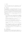
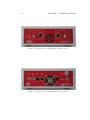
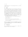
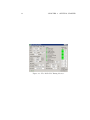
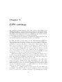
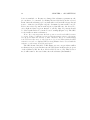
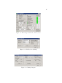
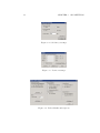
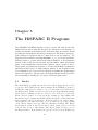
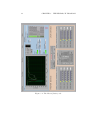
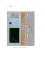
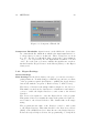
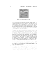
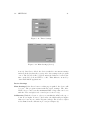
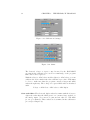
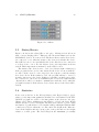
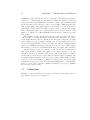
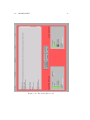
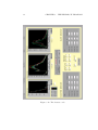
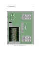
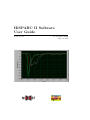
HiSPARC II Software
User Guide
Version 2.1.1
Jeroen van Leerdam
May 28, 2008
2
For information about the HiSPARC project, visit:
http://www.hisparc.nl
This user guide, the HiSPARC II software and other
HiSPARC II information can be found on:
http://www.nikhef.nl/∼jleerdam
Contents
1 Introduction
2 Getting Started
2.1 Hardware . . . . . .
2.2 Software . . . . . . .
2.3 Software Installation
2.4 Databases . . . . . .
2.5 Devices . . . . . . .
2.6 USB Drivers . . . . .
2.7 GPS . . . . . . . . .
2.8 Calibration . . . . .
5
.
.
.
.
.
.
.
.
.
.
.
.
.
.
.
.
.
.
.
.
.
.
.
.
.
.
.
.
.
.
.
.
.
.
.
.
.
.
.
.
.
.
.
.
.
.
.
.
.
.
.
.
.
.
.
.
.
.
.
.
.
.
.
.
.
.
.
.
.
.
.
.
.
.
.
.
.
.
.
.
.
.
.
.
.
.
.
.
.
.
.
.
.
.
.
.
.
.
.
.
.
.
.
.
.
.
.
.
.
.
.
.
.
.
.
.
.
.
.
.
.
.
.
.
.
.
.
.
.
.
.
.
.
.
.
.
.
.
.
.
.
.
.
.
.
.
.
.
.
.
.
.
.
.
.
.
.
.
.
.
.
.
.
.
.
.
.
.
.
.
.
.
.
.
.
.
.
.
.
.
.
.
.
.
3 GPS settings
7
7
8
8
8
9
9
11
11
13
4 Calibration
17
4.1 ADC Alignment . . . . . . . . . . . . . . . . . . . . . . . . . 17
4.2 ADC Calibration . . . . . . . . . . . . . . . . . . . . . . . . . 18
4.3 PMT Calibration . . . . . . . . . . . . . . . . . . . . . . . . . 19
5 The
5.1
5.2
5.3
5.4
5.5
5.6
5.7
HiSPARC II Program
Modes . . . . . . . . . . .
Buttons . . . . . . . . . .
Events . . . . . . . . . . .
Settings . . . . . . . . . .
5.4.1 Events/Settings . .
5.4.2 Expert Settings . .
Status/Errors . . . . . . .
Statistics . . . . . . . . .
Calibration . . . . . . . .
.
.
.
.
.
.
.
.
.
.
.
.
.
.
.
.
.
.
3
.
.
.
.
.
.
.
.
.
.
.
.
.
.
.
.
.
.
.
.
.
.
.
.
.
.
.
.
.
.
.
.
.
.
.
.
.
.
.
.
.
.
.
.
.
.
.
.
.
.
.
.
.
.
.
.
.
.
.
.
.
.
.
.
.
.
.
.
.
.
.
.
.
.
.
.
.
.
.
.
.
.
.
.
.
.
.
.
.
.
.
.
.
.
.
.
.
.
.
.
.
.
.
.
.
.
.
.
.
.
.
.
.
.
.
.
.
.
.
.
.
.
.
.
.
.
.
.
.
.
.
.
.
.
.
.
.
.
.
.
.
.
.
.
.
.
.
.
.
.
.
.
.
.
.
.
.
.
.
.
.
.
21
21
24
25
25
26
29
33
33
34
4
CONTENTS
Chapter 1
Introduction
The HiSPARC project measures muons from cosmic rays on the earth’s
surface with scintillator detectors. The signals from these scintillators are
converted into electrical signals by Photomultiplier Tubes (PMTs). HiSPARC electronics are used in combination with a (personal) computer to
read the PMTs out. In the original setup, the HiSPARC electronics consisted of multiple components and the settings had to be entered with dials
and buttons on the hardware. All the PC had to do, was read out the
(digitised) data and send it to the database.
The components of the HiSPARC electronics are now merged into a
single device. This HiSPARC II device is still read out by a PC, but in the
new setup, the electronics are also controlled by the PC. The settings can
be entered in the LabVIEW software, that sends them to the HiSPARC II
device. One device reads out two PMTs and the HiSPARC II software
can handle two devices at a time (a Master and a Slave), so we can build
detectors with four scintillators.
In this user guide, we describe how to install the HiSPARC II hardware
and software (Chapters 2, 3 and 4) and how to use the software (Chapter 5).
It is assumed that the rest of the detector is already installed—i.e., the
scintillators, PMTs, high voltage cables, signal cables, GPS antenna and
antenna cable are there and are ready to use.
5
6
CHAPTER 1. INTRODUCTION
Chapter 2
Getting Started
This chapter describes how to install and initialise the HiSPARC II hardware and
software. The procedures for initialisation of the GPS receiver and calibration of
the detector are explained in more detail in Chapters 3 and 4, respectively. The
HiSPARC II program can be used with either one or two HiSPARC II devices.
With one device you can use two channels/scintillators and with two devices
you can use four. The installation procedure is the same for both options.
Note: To install the LabVIEW program and device drivers, you must have
administrator rights in Windows.
2.1
Hardware
To use the HiSPARC II hardware, you need:
• a HiSPARC II Master device with power and USB cables
• a HiSPARC II Slave device with power and USB cables (optional)
• two short UTP cables to connect Master and Slave (optional, only if
Slave is used)
• an extra USB cable for the GPS receiver (in the Master )
• a GPS antenna with cable
• a PC with Microsoft Windows XP installed
If you use two HiSPARC II devices, make sure that one of them is a Master
device and the other one is a Slave. The electronics and the software will not
work properly with two Master devices or two Slave devices. The difference
between them is a GPS receiver: The Master has one and the Slave hasn’t.
The GPS antenna connection (Figure 2.2) should not be there on a Slave
device.
7
8
CHAPTER 2. GETTING STARTED
2.2
Software
To control and read out the HiSPARC II hardware, you need the following
software, that is all included in the HiSPARC II software package:
• the HiSPARC II LabVIEW program
• the DSP GPS Timing Monitor software
• FTDI USB drivers
2.3
Software Installation
To install the LabVIEW software (or actually the LabVIEW runtime engine), unzip the HiSPARC II software and go to the Installer directory.
Execute setup.exe and follow the instructions. You have to enter the installation directory for the software here. After installation, you can start
the HiSPARC II program by executing HISPARCII_x_y_z.exe in the installation directory (where x, y and z are the version numbers). The installer
creates a link to this file in the Start Menu.
Note: To use the HiSPARCII software properly, the user that runs the
program must have write permissions for the files in the installation directory and files in the GPS subdirectory. The administrator must either intall
the program in a directory where this is the case, or give the user these
permissions in another directory.
2.4
Databases
Data from a HiSPARC II detector can be stored in two different databases.
There is a Central Database that is located on the Nikhef institute and it is
possible to have a Local Database at the location of the detector, although
the latter is optional. If a Local Database is used, it is recommended to
install it on a machine different from the detector’s. Data from all HiSPARC
detectors in the Central Database can be accessed through the HiSPARC
website. The Local Database is only locally accessible. In general, data
from the devices is sent to both the Local and the Central Database. As
an intermediate step, it is stored in a Buffer Database, that is located on
the same PC as the LabVIEW program. From there it is sent to the other
databases.
To enable LabVIEW to write to this Buffer Database, MySQL must be
installed on the PC to act as a database server and the database should be
created, along with an ODBC Data Source that directs to it. In the future,
all this will be done by the HiSPARC II installer, but for the moment it
has to be done manually. In the rest of this guide, we will assume that the
2.5. DEVICES
9
connection with the Buffer Database is there, although this is not necessary
to run the program and read out the detectors without storing the data.
2.5
Devices
Important: Never plug or unplug the Module I/O USB cables that connect
the HiSPARCII devices to the PC with the device power on. This causes
errors in the operating system USB drivers that Windows cannot handle.
First connect the cables and wait until Windows has started and then swich
the device power on. Switch the power off before unplugging the cables again.
For the USB cable to the GPS receiver, it is the other way around. This cable
must be connected with power on and disconnected before switching off the
Master device.
The following has to be done to install the HiSPARC II devices (see also
Figures 2.1 and 2.2):
1. If you are using two devices, connect them with the two small UTP
cables: One cable from Master LVDS Data Out to Slave LVDS Data
In and the other cable from Slave LVDS Data Out to Master LVDS
Data In.
2. Connect the Module I/O USB port on the device with a USB cable to
the PC. If you are using two devices, connect both.
3. Connect the cable from the GPS antenna to the Master device.
4. Switch the device(s) on: Wait until Windows has started and connect
the power cable from the adaptor to Power In on the device.
5. Connect the GPS Receiver USB port on the Master with a USB cable
to the PC.
6. After the ADC calibration (see Chapter 4), connect the PMT signal
cables to the PMT Inputs on the front of the device: PMT 1 to Master input 1, PMT 2 to Master input 2 and if you are using a Slave
device, PMT 3 to Slave input 1 and PMT 4 to Slave input 2.
7. After the ADC calibration and step 6, connect the PMT control cables
to the PMT Controls.
2.6
USB Drivers
When the devices are used for the first time and the USB cables are connected, Windows will notice and starts a wizard to install the device. If
this wizard asks for a location of the driver files, enter the directory where
10
CHAPTER 2. GETTING STARTED
Figure 2.1: The front of a HiSPARC II (Master ) device
Figure 2.2: The back of a HiSPARC II (Master ) device
2.7. GPS
11
the FTDI USB drivers are located (the USB_drivers directory of the HiSPARC II software).
2.7
GPS
If the HiSPARC II hardware is used for the first time, the GPS receiver
needs to be configured. This process is described in Chapter 3. After this,
every time the Master device is switched on, the GPS receiver needs some
time to track the available satellites and calculate UTC time. You can watch
the status of this process with the DSP GPS Timing Monitor software (see
Figure 2.3). For this you should have connected the GPS receiver port of the
Master device to the PC (as described in Section 2.5). To start the program,
execute GPS\DSPMon.exe in the installation directory. After installation of
the LabVIEW software, there should be a link in the Start Menu. The
monitoring program needs the number of the GPS receiver COM port. You
can change this number by clicking the right mouse button in the lower right
corner of the window (COM6 9600 8-O-1 in Figure 2.3).
The LabVIEW program only receives the right GPS information if:
• all Status lights are green
• the Time is UTC
• the Rcvr Mode in GPS Status is (7) Overdet Clock (Time)
• at least four of the satellite (SV ) numbers in Signal Levels are green
(more is recommended)
Make sure you check this every time you restart the Master device and before
you start the LabVIEW program to take data. The GPS information is not
needed for the calibration procedure, so you don’t have to check this before
starting the calibration process.
2.8
Calibration
Before a HiSPARC II device can be used, it needs to be calibrated. The
calibration procedure is described in Chapter 4.
12
CHAPTER 2. GETTING STARTED
Figure 2.3: The DSP GPS Timing Monitor
Chapter 3
GPS settings
For comparison between detectors, each event is given a time stamp by the
HiSPARC II hardware. To ensure that each event receives a correct time stamp,
the Global Positioning System is used for synchronisation of the detector clocks.
Each Master device has a GPS receiver to communicate with the GPS satellites.
In this chapter we describe how to configure this receiver.
It is assumed that the installation, as described in Chapter 2, is done. We
will use the information from Sections 2.3 and 2.7 in particular.
To change the GPS receiver settings, both the HiSPARC II LabVIEW software and the DSP GPS Timing Monitor are needed. The LabVIEW program runs immediately after the executable is started. A dialog box appears,
in which you can select the mode for this session. This should be Expert
Mode. You are prompted for a password, but if there is no password set yet,
you can just click OK here. After the GPS configuration is done, you can
exit the program by clicking the Stop Program button (see Figures 5.1 and
5.2 on pages 22 and 23). Do not save settings at exit. See Chapter 2, Section 2.3 and Chapter 5 for more information about the LabVIEW program
and Chapter 2, Section 2.7 for the DSP GPS Timing Monitor.
Changes in the GPS settings can be made by pushing the Enable writing
to GPS receiver and the Apply Settings buttons on the Expert Settings page
in the HiSPARC II LabVIEW program (Figure 5.2). The GPS settings can
now be written with the GPS monitoring program.
Set the GPS Receiver, Timing Outputs, Self-Survey, Position and Packet
Masks and Options settings in the Setup menu (Figure 3.1) to the values
indicated in Figures 3.2 to 3.6. If you change any values (most of the default
values should be correct), do not forget to push the save buttons (Set SV, Set
Receiver, Set PPS, Set Qualifier, . . . ). When this is done, save the settings
with Save Configuration in the Setup menu.
In the Position settings, we did not set an Accurate Position. This position must be determined by the receiver in a self-survey. If the receiver has
never been used before, a self-survey is started automatically if the Master
13
14
CHAPTER 3. GPS SETTINGS
device is switched on. Because we changed the self-survey parameters, the
process has to be restarted by clicking Restart Self-Survey in the Control
menu. After the self-survey process, that takes one hour if the Survey-Length
is set to 3600 fixes (see Figure 3.4), the determined position will be stored.
If for some reason a position is already stored (in this case, the Stored Position light in Status is green instead of yellow), this old position should
be deleted with Delete Pos in the Position settings (Figure 3.5). The GPS
receiver will now start a self-survey.
Note: It is very important that the position stored in the GPS receiver
is correct. If the coordinates are wrong, the timestamps given to the events
are off by an unknown amount of time. However, this is not immediately
noticed, because the error is only a fraction of a second. Every time the GPS
antenna is moved or a different GPS receiver/ Master device is used with the
antenna, a self-survey should be performed.
The GPS monitor should look like Figure 2.3 now, except if there still is
a self-survey in progress. In that case the GPS Status indicates the progress
of the self-survey and the Rcvr Mode is Full Position (3D). This receiver
mode will return to the saved value after the self-survey has finished.
15
Figure 3.1: The Setup menu in the GPS monitor
Figure 3.2: GPS Receiver settings
Figure 3.3: Timing Outputs
16
CHAPTER 3. GPS SETTINGS
Figure 3.4: Self Survey settings
Figure 3.5: Position settings
Figure 3.6: Packet Masks and Options
Chapter 4
Calibration
To send the signal on the analog inputs of a device to the computer, it needs to
be digitised. This is done with four 12-bit ADCs (two per channel), that measure voltages from approximately 0 to 2 V 1 . To make sure all ADCs give the
same digital value for a certain voltage applied to the inputs and to determine
what that particular value is, the device needs to be calibrated. This has to be
done for both the Master and the Slave device (if you are using one). After
the calibration is completed, it is necessary to make sure that all the scintillator/PMT combinations give the same response for a given particle that goes
through the detector. This is done by adjusting the PMT high voltages.
To get the best results, the PMT calibration (Section 4.3) should be performed after the ADC alignment (Section 4.1), with the default values for the
ADC calibration (Section 4.2). Then, after the device(s) has (have) been taking
data for several hours (without writing to the database), the full ADC calibration should be done and the PMT calibration should be done again. This makes
sure that the whole detector is on “operation temperature” during calibration.
In this chapter it is again assumed that the installation as described in Chapter 2
has been completed.
4.1
ADC Alignment
To make sure that all the ADCs (in one device) have the same scale and give
the same value for a given voltage, they have to be aligned. This alignment
can be performed with the HiSPARC II LabVIEW program. When the
program is started, it runs immediately and a dialog box appears, in which
the user can select the mode to run in. This mode should be Expert Mode
for the calibration procedure. You are now prompted for a password, but if
no password is set yet, you can just click OK here. After the calibration,
1
The signal from the PMTs is actually a negative voltage, but before it is digitised, it
is converted to a positive voltage. −1 V at the analog input corresponds to +1 V at the
ADC.
17
18
CHAPTER 4. CALIBRATION
you can exit the program with the Stop Program button (see Figures 5.1
and 5.2 on pages 22 and 23).
Now first make sure that nothing is connected to the analog inputs of the
devices (the PMT Inputs in Figure 2.1 on page 10). Go to the Calibration
tab page of the program (Figure 5.18 on page 37) and push the Start Calibration button. The alignment process is now started and the calibration
parameters in the lower left and lower right corners of the screen should
be changing. (Obviously, if only a Master is used, only the Master values
change.) The alignment is performed in six steps, so it finishes when the
Calibration Steps in the upper right corner of the screen reach seven. Select
Yes (save calibration settings) in the dialog box that appears.
Note: the settings are not saved to the device, but on the PC hard disk.
If you use another device with the same PC, the calibration procedure must
be repeated.
4.2
ADC Calibration
After the alignment process, one has to determine the scale and offset of
the ADCs. These quantities are represented by the Gain for ADC values
and Offset for ADC values controls on the Calibration tabs on the Expert
Settings tabpage (see Figure 5.2 on page 23 and Figure 5.13 on page 32).
These controls have to be set for each channel (so two times for each device).
After alignment the values should be approximately −0.57 mV and 114 mV ,
respectively, which are the default values. The voltage on the analog input
on the device is calculated with:
Voltage = ADC Gain · ADC value + ADC Offset
(4.1)
The Gain for ADC values and Offset for ADC values should be set
correctly on the Calibration tab pages, because the HiSPARC II program
uses these values to calculate other device settings and to display events.
If it is for some reason impossible to perform the calibration procedure
described in this section, you can use the default values (after aligning with
the HiSPARC II program), although this is not recommended.
The ADC calibration values can be determined by applying a (known)
voltage to the analog inputs of the device and reading off the corresponding
ADC value from the output of the HiSPARC II program. After (a minimum
of) two of these measurements (at different voltages), the Gain for ADC
values and the Offset for ADC values can be calculated with Equation 4.1.
For the voltage–ADC measurements, the Gain for ADC values should
be temporarily set to 1.0000 and the Offset for ADC values to 0.0. To do
this, enter the values in the controls and push the Apply Settings button
(see Figure 5.2 on page 23 and Figure 5.3 on page 25). For these settings,
the voltage that is displayed in the graphs on the Events/Settings tab and
4.3. PMT CALIBRATION
19
the Expert Settings tab is equal in value to the ADC output. If a DC voltage
is applied to the inputs, this will appear in the graphs as a line at a certain
ADC value. The device(s) should be triggered to show this line in events. To
do this, set the Trigger Condition on the Events/Settings–Trigger Settings
tab page (Figures 5.1 and 5.4 on pages 22 and 26) to Use only the external
trigger and push the Apply Settings button again. Now apply a positive
pulse between 0 and 3 V and a length in the order of microseconds to the
Ext. Trig. In input at the back of the Master device (see Figure 2.2 on
page 10). Repeat the pulse every second or so. Each time this trigger is
given, an event should appear on the screen and the ADC value can be read
off. Use values for the DC voltage of ≈ −30 mV and ≈ −2000 mV and if you
want more measurements, values in between. After calculating the ADC
calibration values, do not forget to enter them on the Expert Settings tab
page (and to push the Apply Settings button). The settings can be saved
by pushing the Save Settings button.
4.3
PMT Calibration
Now that the devices are calibrated, we can take a look at the signals from
the scintillators/PMTs. We have to calibrate this part of the detector as
well, because each PMT behaves differently for a given high voltage applied
to it. When a muon goes through a scintillator plate, it causes a pulse at
the output of the PMT. For the calibration we will assume that this pulse is
completely characterised by the maximum height it reaches (or actually the
maximum depth, because the PMT’s pulses are negative). Because we deal
with statistical processes and this pulse height depends on the energy of the
muon, the signal will be different for each particle that goes through the
detector. However, a histogram of pulse heights over a long enough time,
should always be the same. In approximation, these histograms only depend
on the high voltage applied to the PMT; the higher the voltage, the more
“high pulses” we get and the more the histogram shifts to the right. What
we want to do now is making sure that we get the same histogram for all
the PMTs.
If we would count the number of pulses that exceed a certain threshold
pulse height in a given amount of time, we are actually measuring the surface
of the pulse height histogram to the right of this threshold. If we make sure
that the count/surface for a given threshold is the same for each PMT, the
pulse height histograms are the same. We can adjust the count/surface by
adjusting the PMT high voltage. The higher the voltage, the more counts
we get.
Connect the cables from the PMTs to the front of the device(s), as
described in Chapter 2, Section 2.5. Set the trigger to Use only the external
trigger again (as in Section 4.2). We can set our theshold pulse height
20
CHAPTER 4. CALIBRATION
on the Events/Settings–Thresholds tab pages (Figure 5.6 on page 28). The
program uses two thresholds: a low one and a high one. Set the low threshold
to 250 mV and the high threshold to 300 mV . (You can enter these values
in the boxes to the right of the slide controls.) Do this for each channel (so
two times for each device). Now go to the Events/Settings–Photomultiplier
Tube tabs (Figure 5.8 on page 28) and set the PMT High Voltage Adjusts to
800 mV (this corresponds to approximately 800 V at the PMT). Push the
Apply Settings button to send these values to the device(s).
On the Statistics tab page (Figure 5.17 on page 36) you can count the
number of times each channel went over the thresholds. The grey panels
at the bottom of the page show in the left column the number of times the
signal went over the thresholds in the last second. If you push the Start
Counting button in the middle, the middle column shows the total number
of counts and the right column the average per second. You can set the
number of seconds to count with the Time to count control.
Count for about 30 seconds and check the averages. For the low thresholds (250 mV ) this should be between 50 and 60 counts/s and for the high
thresholds (300 mV ) between 30 and 40 counts/s. If this is not the case,
adjust the PMT High Voltage Adjusts (do not forget the Apply Settings
button) and repeat the measurement until all averages are within the given
range. Now count again for 300 seconds and check if the averages are still
right.
When the calibration is finished, push the Save Settings button to save
all settings to the hard disk. You can exit the program by pushing the
Stop Program button. Check the values for the high voltage again when
the program is taking data: If the trigger is set to At least 2 low signals or
At least 2 high signals (4 low and 4 high if you are using two devices), the
Pulse Height Histograms on the Statistics page should be the same for all
the channels and have a peak at ≈ 400 counts (≈ 230 mV ). You can find an
example of the Pulse Height Histograms in Figure 5.17, although this is for
a different trigger condition, so the Master –Channel 2 histogram is not the
same as the histograms for the other channels.
Chapter 5
The HiSPARC II Program
The HiSPARC II LabVIEW program is used to control and read out the HiSPARC II devices and to send the data from the detectors to the database. It
needs to be installed on the detector’s PC and before usage, the detector should
be calibrated as described in the previous chapters. In this chapter, all the program settings are explained and it is shown how to use the software. The
program can be started by executing HISPARCII_x_y_z.exe in the installation
directory (where x, y and z stand for the version numbers). In the installation
process, a link to this file was created in the Start Menu. When the program
starts, it runs immediately and the user is asked to select a mode to run in.
These modes are explained in Section 5.1. For the Expert Mode a password is
required, but this is set to an empty string by default, so just click OK if there
is no password set yet. You can exit the program by pushing the Stop Program
button (see Figure 5.1). After the exit, the program window is still open and it
can be restarted by clicking the “run arrow” in the left upper corner.
5.1
Modes
The HiSPARC II program can run in Normal Mode, Expert Mode or Data
Acquisition Mode (DAQ Mode). After starting the LabVIEW program (or
clicking the “run arrow”) you have to choose between the Normal Mode and
the Expert Mode. When you select a version, the program will start running
(after it gives a warning if only one device is or no devices are connected).
In the Normal version, you can set all the settings for data taking, like
thresholds, trigger settings and PMT settings and write events taken with
these settings to the Local Database. In Normal Mode you cannot change
any settings for the DAQ Mode and you do not have access to the settings
on the Expert Settings tab page, like the calibration settings. The Expert
Mode runs the same as the Normal Mode, but is password protected and
now you have access to all settings. The Expert password can be set on
the Expert Settings–Main Settings tab page (see Section 5.4.2). Finally, the
21
22
CHAPTER 5. THE HISPARC II PROGRAM
Figure 5.1: The Events/Settings tab
5.1. MODES
23
Figure 5.2: The Expert Settings tab
24
CHAPTER 5. THE HISPARC II PROGRAM
DAQ Mode is for long term data taking. In this mode the events are written
to both the Central and the Local Database (if there is one) and it is not
possible to change any settings while the program is in DAQ Mode.
The Normal Mode and the Expert Mode each have their own settings file
on the hard disk to which settings can be saved. When the Save Settings
button is pushed, it depends on the mode the program runs in to which
file the settings are saved. The Expert, however, is able to write to the
Normal file as well (see also Section 5.2). When the program starts, it loads
the settings of the mode it is started in. The DAQ Mode uses the Expert
Settings.
5.2
Buttons
In Figures 5.1 and 5.2 the Settings tabs of the program are shown. In the
middle you can see a panel with six buttons. (Figure 5.3) This panel is
visible at all the tabs and contains the main controls of the program.
Stop Program This button stops the running of the program. After pushing it, a dialog is shown in which you can choose to run again or to
exit the program.
DAQ Mode After pushing this button, the program will restart and go
into DAQ Mode. Data will be written to all databases. Pushing the
DAQ Mode button while the program is in DAQ Mode will result in
a restart to the “select mode dialog”.
Apply Settings All settings values (with the exception of the Write to
local DBase button) can be changed without having immediate effect.
Only after pushing Apply Settings, the new settings are processed and
sent to the device(s).
Save Settings Pushing this button will save all current settings to the hard
disk. When you restart after saving, the saved settings are restored.
Save Settings writes the settings as they were at the last time that
Apply Settings was pushed, so always apply first and then save.
Reset This button restores the default factory settings. Pushing it results
in loss of all current settings. (This only affects the settings of the
mode you are in.)
Write to local DBase? If this button is pushed and the light is on, all
measured and processed data is written to the Local Database. Pushing
this button has immediate effect, so there is no need to push the Apply
Settings button, except if you want to save the Write to local DBase
setting (see also Save Settings).
5.3. EVENTS
25
Figure 5.3: Buttons
On the Expert Settings tab page (Figure 5.2) there is another Save Settings button, to the right of the main six:
Save Settings (to Normal Settings) This second Save Settings button,
that is only on the Expert Settings page, saves the current Expert
Settings to the Normal Settings. This has no effect on the saved Expert
Settings, but the old Normal Settings will be lost.
5.3
Events
Every time there has been a trigger and the device recorded the input signals
for a number of microseconds (see also Section 5.4.1), an event is shown on
the Events/Settings and Expert Settings tab pages and is written to the
database (if the program is in DAQ Mode or if it is writing to the Local
Database). An event consists of two or four traces (dependent on whether
you are using two devices or not), a GPS time stamp, a trigger pattern and
a detector number.
The Traces contain the measured ADC data and this is plotted on the
screen. The GPS timestamp shows the date and time of the event. The
Trigger pattern shows over which thresholds the input signal went at the
time of the trigger and whether there was a Slave device present or not.
The Detector number is the unique number set on the Expert Settings–
Detector Settings tab. On the Events panels the current Status, the harware
and software Version numbers and the coordinates of the GPS antenna are
shown as well.
5.4
Settings
Besides displaying recorded events, the Events/Settings and Expert Settings
tabs also contain the controls for all the settings of the device(s). There
are two types of settings: general settings and device settings. You can set
the same settings on the Slave device as you can set on the Master, but
the values can be different. The general settings apply to both the Master
and the Slave device, or only to the HiSPARC II program itself. You can
change the settings on the Events/Settings tab in both the Normal Mode as
26
CHAPTER 5. THE HISPARC II PROGRAM
Figure 5.4: Trigger Settings
the Expert Mode and the settings on the Expert Settings tab only in Expert
Mode.
5.4.1
Events/Settings
General Settings
Trigger Settings If a signal at the analog input exceeds its threshold value
(see the Thresholds tab), a signal is sent to the trigger system, which
decides whether to record an event or not. At this tab you can set
under which condition this happens. You can use the internal (thresholds) system, the external trigger (an input on the devices) or both.
For the internal trigger you can set the minimum number of high and
low over-threshold signals there must be before the device starts taking data. If you use only a master device the maximum number of
signals you can get is obviously two. With the and/or switch you can
set whether you want at least n low signals and m high signals or at
least n low signals or at least m high signals.
Time Window If there is a trigger, the device starts recording the input
signals for a specified time. On this tab you can set the time it records
before the time of the trigger (Pre Coincidence Time), the time within
which all over-threshold signals must come to cause a trigger (Coincidence Time or Trigger Window ) and the time it measures after the
Coincidence timewindow (Post Coincidence Time). The Coincidence
Time also counts for the total measuring time, so the total time is the
sum of these three. The Pre Coincidence Time can be set from 0 to
2 µs, the Coincidence Time from 0 to 5 µs and the Post Coincidence
Time from 0 to 8 µs. The total time cannot be more than 10 µs. Although it is possible to use a Pre Coincidence Time down to zero, this
is not recommended. If the Pre Time is smaller than 0.125 µs, the
5.4. SETTINGS
27
Figure 5.5: Time Windows
baseline of the signal cannot be determined and the histograms on the
Statistics page will not be filled (see also Section 5.6).
Device Settings
Thresholds The thresholds give the values above which (or actually below
which, because all voltages are negative) the signals on the analog
inputs of the device(s) cause a signal in the trigger system. The trigger
system then decides whether the device starts recording data or not.
Each channel has its own threshold values and you can set both a low
value and a high value. (See Trigger Settings for more information
about the low and high values.) The Statistics tab page (Section 5.6
and Figure 5.17) shows how many times the input signal was above
the threshold in the last second.
Warning: The threshold values are set in mV , but this is only correct
if the device is calibrated and the right gain and offset values are set on
the Expert Settings–Calibration tabs (see Chapter 4 for calibration).
Integrator Times Here the RC time constant of the integrator circuit at
the analog inputs can be set. The controls can be set from 0 to 255,
where 0 corresponds to a large RC time and 255 to a short RC time.
Photomultiplier Tube On the photomultiplier tube page the high voltage
that is applied to the tube can be set. The voltage supplied by the
HiSPARC II device is set in mV and transformed at the tube to a high
voltage. The factor between the voltage at the device and the high
voltage is approximately 1000. The voltage can vary from 300 mV to
1500 mV , but the maximum voltage you can apply is set on the Expert
Settings–Main Settings tab. This tab also shows the supply current
for each tube.
28
CHAPTER 5. THE HISPARC II PROGRAM
Figure 5.6: Thresholds
Figure 5.7: Integrator Times
Figure 5.8: Photomultiplier Tube
5.4. SETTINGS
29
Figure 5.9: Comparator Thresholds
Comparator Thresholds Apart from two at the ADCs, the devices have
two extra thresholds, which show whether the input signal was above
a voltage that you can set on this tab. These voltages are set from
0 to 255. For the low threshold, this corresponds to approximately
−2 V to −7 V , respectively. For the high threshold, this is −2 V and
−11 V . For each event, you can see whether the signal went over these
thresholds in the Trigger Pattern on the Events/Settings or the Expert
Settings tab.
5.4.2
Expert Settings
General Settings
Main Settings On the Main Settings tab page, you can set several program parameters. To make changes on this tab page effective, a restart
of the program is required (in addition to pushing the Apply Settings
button and with the exception of Enable writing to GPS receiver ).
The Detector Number is the unique number assigned to the detector.
This number is used in the databases for identification and must be
correct to enable the Buffer Database to send events to the Central
Database.
The Password is required to enter the Expert Mode of the program.
This password is not necessarily the same as the password required to
send events to the Central Database. The default value is an empty
string.
The program uses the value of the Database control to send events
to the Buffer Database. This value should be the Data Source Name
(DSN ) of the ODBC Data Source that directs to the Buffer Database.
If Start directly in DAQ mode is set, the program will go to DAQ Mode
30
CHAPTER 5. THE HISPARC II PROGRAM
Figure 5.10: Main Settings (general)
as soon as it is started and skips the dialogs that usually appear. You
can use this setting if the PC is configured to automatically logon to
Windows and to start the HiSPARC II program at logon. This way,
the program will automatically resume taking data after a restart of
the PC. This is often desirable for long term data taking, as Windows
has a habit of forcing a reboot after an automatic update. If the PC
can also be configured to automatically power up after a power failure,
only a crash can stop the data acquisition.
The Filter data? and Use filter threshold checkboxes control the filtering of the digital signals in the HiSPARC II software. Filtering is
necessary for a number of HiSPARC II devices that have a flaw in
the electronics. This flaw causes an oscillation in the analog input
signal that is filtered out if Filter data? is set. Because the filtering
has not the desired effect for large fluctuations of the input signal, a
filter threshold is used. This threshold is controlled by the Use filter
threshold checkbox. The software stops filtering if the fluctuation in
the signal exceeds the threshold. If a device with the flaw is used,
the filter should be used with a threshold, i.e.—both boxes should be
checked. For devices without the flaw, the filter should not be used.
Enable writing to GPS receiver is the only control for which a change
is effective immediately after pushing the Apply Settings button. This
control enables or disables writing the GPS receiver settings (see Chapter 3). If you are not adjusting these settings, writing should be disabled (light on the button off ).
Timer Settings On this tab page you can set the minimum time between
Screen Updates, between Device Checks (both in seconds) and between
PC Clock Error Updates (in minutes). The screen is only updated if
there are new events or new Second Messages from the device, which
contain the Singles information on the Statistics tab page (see Sec-
5.4. SETTINGS
31
Figure 5.11: Timer Settings
Figure 5.12: Main Settings (device)
tion 5.6). In a Device Check, the device is asked for its current settings
and it is checked wether they correspond to the settings of the program
or not. The PC Clock Error Update writes the difference between the
time on the PC clock and UTC to a file. This difference is used by
other HiSPARC II applications.
Device Settings
Main Settings If the Reset button on this page is pushed, the device will
be reset. The program restarts with the saved settings. The Max.
PMT voltage control sets the maximum PMT voltage that can be set
with the Photomultiplier tube controls (see Section 5.4.1).
Calibration With the Common offset you can shift the ADC scale up or
down. For a higher Common offset value, the ADCs will give higher
values (or lower if you consider negative values). The Common Offset
is determined in the calibration process (see Chapter 4).
32
CHAPTER 5. THE HISPARC II PROGRAM
Figure 5.13: Calibration Settings
Figure 5.14: Gains
The Internal voltage on inputs control is used by the HiSPARC II
program in the calibration process. For normal usage of the program
this control can be ignored.
With the Gain for ADC values and the Offset for ADC values, you can
calibrate the device further after the calibration procedure. This must
be done to make sure that the program converts voltages and ADC
values the right way. The voltage for a given ADC value is calculated
with:
Voltage = ADC Gain · ADC value + ADC Offset
Gain and Offset The Gain and Offset values determine with the Common
Offset the value that the ADC gives for a certain voltage applied on
the analog input. You can set a gain and an offset for each ADC
(so two per channel). These values are determined in the calibration
process (see Chapter 4).
5.5. STATUS/ERRORS
33
Figure 5.15: Offsets
5.5
Status/Errors
Figure 5.16 shows the Status/Errors tab page. Messages from all errors
that occur are displayed here. This page also shows information about the
HiSPARC II devices. You can see here whether a Master and a Slave device
are connected or not, what the status of the devices is, whether the device
has a GPS receiver or not and whether the device has detected a connection
to a Slave device or not. For the Master device, its temperature is shown
as well. This temperature is measured on the GPS receiver.
The status of the device is set to “bad” (a red Status light on this page)
if the program did not receive any data from the device for more than two
seconds or if the device does not respond to the request to send its settings
in a device check. If the status is “bad” the program will try to restore a
normal connection to the devics. If this process times out after ten seconds,
the connection to the device is terminated (the Connected? light switches
off) and there will be no further communication with the device until the
program is restarted. If the Master device is disconnected, the Slave will be
as well.
5.6
Statistics
If an event is shown on the Events/Settings and Expert Settings pages,
values of a few important quantities calculated for each channel by the HiSPARC II program are added to the histograms on the Statistics tab page
(Figure 5.17). These quantities are the Number of Peaks, the Pulse Height
and the Integral of a recorded signal. The Histogram number of peaks counts
the number of peaks in the recorded signal. Only peaks higher than 60 ADC
counts (≈ 35 mV ) are taken into account, where the height is the difference
between the highest and the lowest point of the peak and not the height
relative to a fixed point. The Pulse Height is the maximum (or actually
34
CHAPTER 5. THE HISPARC II PROGRAM
minimum) of the signal in the full recorded time. This value is calculated
relative to a baseline, that is determined by taking the average of the first
data points, where the PMT still is at its base voltage. The third histogram
shows the values of the Integral of the recorded signal. This integral is the
sum of the heights of the signal relative to the baseline, for each point where
this height is larger than four ADC counts (≈ 2 mV ). All the histograms
have a maximum value, above which entries are no longer plotted. The
number of entries above this maximum is shown in the counters below the
histograms.
The baselines are also shown on the Statistics page for each event. These
values should be around 200 ADC counts after the calibration procedure.
If the signal already varies too much in the first data points, the program
can’t calculate a proper baseline. In that case, it tries again at the end of
the recorded signal. If this doesn’t work either, the values for the histograms
cannot be calculated and the program gives an error for the baseline (-999).
The number of errors for each channel is shown to the right of the baselines.
On the Statistics page you can also see the Singles for each threshold.
This is the number of times the signal on the analog inputs exceeds the
threshold. In the left column on the Singles panel, the number of singles
in the last second is shown. If the Start Counting button is pushed, the
program counts the singles for a longer period of time. In the middle column,
you can see the total number of singles over this period and in the right
column the average per second. You can set maximum time to count with the
Time to count control, but the counting can always be stopped by pushing
the Counting button again.
5.7
Calibration
In Figure 5.18, the Calibration tab page is shown. For information about
the calibration process, see Chapter 4.
5.7. CALIBRATION
Figure 5.16: The Status/Errors tab
35
36
CHAPTER 5. THE HISPARC II PROGRAM
Figure 5.17: The Statistics tab
5.7. CALIBRATION
Figure 5.18: The Calibration tab
37