1
MRT User Manual
Politecnico di Milano, Dept. of Electronics and Information
AIRLab, Artificial Intelligence and Robotics Laboratory
Luigi Malag`o
September 15, 2007
Contents
1 Introduction
6
2 Modular Robotic Toolkit
2.1 Functional Modules . . . . . . . . . .
2.2 Middleware for Modules Integration
2.3 Applications . . . . . . . . . . . . . .
2.3.1 Roby . . . . . . . . . . . . . .
2.3.2 FollowMe . . . . . . . . . . .
2.3.3 Milan RoboCup Team . . . .
.
.
.
.
.
.
.
.
.
.
.
.
.
.
.
.
.
.
.
.
.
.
.
.
3 Device Communities Development Toolkit
3.1 Agora and Members . . . . . . . . . . . . .
3.2 Messages . . . . . . . . . . . . . . . . . . .
3.3 Configuration Files and Examples . . . . .
3.3.1 Agora . . . . . . . . . . . . . . . . .
3.3.2 Members . . . . . . . . . . . . . . .
3.3.3 Messages . . . . . . . . . . . . . . .
.
.
.
.
.
.
.
.
.
.
.
.
.
.
.
.
.
.
.
.
.
.
.
.
.
.
.
.
.
.
.
.
.
.
.
.
.
.
.
.
.
.
.
.
.
.
.
.
.
.
.
.
.
.
.
.
.
.
.
.
.
.
.
.
.
.
.
.
.
.
.
.
.
.
.
.
.
.
.
.
.
.
.
.
.
.
.
.
.
.
.
.
.
.
.
.
.
.
.
.
.
.
.
.
.
.
.
.
.
.
.
.
.
.
7
8
10
11
11
13
13
.
.
.
.
.
.
17
17
19
20
20
23
26
4 Mice
27
4.1 The Odometry Sensor and Pose Estimation . . . . . . . . . . 28
4.2 Sensor Error Detection and Reduction . . . . . . . . . . . . . 31
4.3 TODO Configuration Files and Examples . . . . . . . . . . . 32
5 AIRBoard
5.1 Hardware and
5.2 The board . .
5.3 Control . . .
5.4 The driver . .
Sotfware Design
. . . . . . . . . .
. . . . . . . . . .
. . . . . . . . . .
.
.
.
.
.
.
.
.
.
.
.
.
.
.
.
.
.
.
.
.
.
.
.
.
.
.
.
.
.
.
.
.
.
.
.
.
.
.
.
.
.
.
.
.
.
.
.
.
.
.
.
.
.
.
.
.
.
.
.
.
.
.
.
.
.
.
.
.
33
34
34
35
35
6 RecVision
36
7 MUlti-Resolution Evidence Accumulation
37
8 Map Anchors Percepts
38
1
9 Spike Plans in Known Environments
39
10 Multilevel Ruling Brian Reacts by Inferential ActioNs
10.1 The Behavior-based Paradigm . . . . . . . . . . . . . . . . . .
10.2 The Overall Architecture . . . . . . . . . . . . . . . . . . . .
10.2.1 Fuzzy predicates . . . . . . . . . . . . . . . . . . . . .
10.2.2 CANDO and WANT Conditions . . . . . . . . . . . .
10.2.3 Informed Hierarchical Composition . . . . . . . . . . .
10.2.4 Output Generation [—–questa sezione ci sta o no? e’
una ripetizione di cose appena dette? e’ coerente con
quanto c’e’ sopra per le formule e le convenzioni nei
nomi delle variabili?——] . . . . . . . . . . . . . . . .
10.3 Modules??? [———-vanno bene anche per Mr. BRIAN?? il
disegno e il flusso dei dati e’ corretto?——–] . . . . . . . . . .
10.3.1 Fuzzyfier . . . . . . . . . . . . . . . . . . . . . . . . .
10.3.2 Preacher . . . . . . . . . . . . . . . . . . . . . . . . . .
10.3.3 Predicate Actions [——-questo capitolo e’ qui, anche se non corrisponde ad un particolare modulo di
Mr.Brian. Chi si occupa delle predicate actions? Lo
lascio qui o lo sposto? Se lo sposto, dove lo metto?——]
10.3.4 Candoer . . . . . . . . . . . . . . . . . . . . . . . . . .
10.3.5 Wanter . . . . . . . . . . . . . . . . . . . . . . . . . .
10.3.6 Behavior Engine . . . . . . . . . . . . . . . . . . . . .
10.3.7 Rules Behavior . . . . . . . . . . . . . . . . . . . . . .
10.3.8 Composer . . . . . . . . . . . . . . . . . . . . . . . . .
10.3.9 Defuzzyfier . . . . . . . . . . . . . . . . . . . . . . . .
10.3.10 Parser and Messenger . . . . . . . . . . . . . . . . . .
10.4 Configuration Files and Examples . . . . . . . . . . . . . . .
10.4.1 Fuzzy Sets . . . . . . . . . . . . . . . . . . . . . . . . .
10.4.2 Fuzzy Predicates . . . . . . . . . . . . . . . . . . . . .
10.4.3 Predicate Actions . . . . . . . . . . . . . . . . . . . . .
10.4.4 CANDO and WANT Conditions . . . . . . . . . . . .
10.4.5 Playing with activations TODO . . . . . . . . . . . . .
10.4.6 Defuzzyfication . . . . . . . . . . . . . . . . . . . . . .
10.4.7 Behavior Rules . . . . . . . . . . . . . . . . . . . . . .
10.4.8 Behavior List . . . . . . . . . . . . . . . . . . . . . . .
10.4.9 Behavior Composition . . . . . . . . . . . . . . . . . .
10.4.10 Parser and Messenger . . . . . . . . . . . . . . . . . .
10.4.11 Using Mr. BRIAN . . . . . . . . . . . . . . . . . . . .
40
41
41
43
44
46
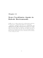
11 Scare Coordinates Agents in Robotic Environments
79
2
47
48
51
52
52
53
54
54
55
56
57
58
58
60
62
64
66
67
68
70
71
72
73
76
12 Milan RoboCup Team ?????? per adesso rimane in
12.1 RoboCup Soccer . . . . . . . . . . . . . . . . . . . .
12.2 Leagues . . . . . . . . . . . . . . . . . . . . . . . . .
12.3 Middle Size League Regulation and Rules . . . . . .
12.4 The Robot Team . . . . . . . . . . . . . . . . . . . .
12.5 The IANUS3 base . . . . . . . . . . . . . . . . . . .
12.6 The Triskar base . . . . . . . . . . . . . . . . . . . .
12.7 Sensors . . . . . . . . . . . . . . . . . . . . . . . . .
3
sospeso
. . . . .
. . . . .
. . . . .
. . . . .
. . . . .
. . . . .
. . . . .
80
81
82
83
83
84
85
85
List of Figures
2.1
2.2
2.3
2.4
The general architecture implemented by the MTR . . . . . . 10
MRT modules involved in the Roby case study . . . . . . . . 12
Modules involved in the FollowMe architecture . . . . . . . 14
Modules involved in the MRT architecture for the Milan RoboCup
Team . . . . . . . . . . . . . . . . . . . . . . . . . . . . . . . . 15
3.1
3.2
Structure of the Agora . . . . . . . . . . . . . . . . . . . . . .
Inter Agora communication. [——–questa figura probabilmente non va bene... mancano dei componenti forse, tipo
LinkTX e LinkRx in Agora1. Inoltre le Agora vanno scritte
con il numero attaccato al nome, es Agora1 e non Agora 1—
—-] . . . . . . . . . . . . . . . . . . . . . . . . . . . . . . . . .
4.1
4.2
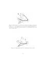
The angle arc of each mouse is equal to the change in orientation of the robot [—–forse angle arc non va bene, ma la stessa
didascalia che c’ in un articolo di Bonarini e Restelli e Matteucci, A kinematic-independent dead-reckoning sensor...—-] .
The triangle made up of joining lines and two radii . . . . . .
10.1
10.2
10.3
10.4
10.5
Mr. BRIAN architecture . . . . . . . . . . . . . . . . . . . . .
Mr. BRIAN module functional structure . . . . . . . . . . . .
Mr. BRIAN modules working structure . . . . . . . . . . . .
Fuzzy sets available in Mr. BRIAN . . . . . . . . . . . . . . .
The predicate actions flow of information between the hierarchy of levels . . . . . . . . . . . . . . . . . . . . . . . . . .
10.6 Behavior Engine structure . . . . . . . . . . . . . . . . . . . .
10.7 Composer working structure . . . . . . . . . . . . . . . . . . .
10.8 Barycenter defuzzyfication . . . . . . . . . . . . . . . . . . . .
10.9 Representation of the Distance shape and example of fuzzification . . . . . . . . . . . . . . . . . . . . . . . . . . . . . . .
10.10Representation of a complex predicate . . . . . . . . . . . . .
10.11(a) GoToTarget trajectory (b) GoToTarget and AvoidObstacle trajectory . . . . . . . . . . . . . . . . . . . . . . . . . . .
4
18
22
29
29
42
49
50
51
53
54
56
57
62
64
68
10.12Representation of the SPEEDMODULE shape and example
of defuzzyfication . . . . . . . . . . . . . . . . . . . . . . . . .
70
12.1
12.2
12.3
12.4
12.5
84
85
86
86
86
The
The
The
The
The
IANUS3 base . . . . . . . . . . . . . .
Triskar base: front side . . . . . . . . .
Triskar base: back side . . . . . . . . .
omnidirectional vision system . . . . .
two USB optical mice on the bottom of
5
. . . . .
. . . . .
. . . . .
. . . . .
the base
.
.
.
.
.
.
.
.
.
.
.
.
.
.
.
.
.
.
.
.
.
.
.
.
.
Chapter 1
Introduction
This is the Modular Robotic Toolkit user manual, a comprehensive guide to
the software architecture for autonomous robots developed by the AIRLab,
Artificial Intelligence and Robotic Laboratory of the Dept. of Electronics
and Information at Politecnico di Milano.
MRT, Modular Robotic Toolkit, is a framework where a set of off-theshelf modules can be easily combined and customized to realize robotic applications with minimal effort and time. The framework has been designed to
be used in different applications where a distributed set of robot and sensors
interact to accomplish tasks, such as: playing soccer in RoboCup, guiding
people in indoor environments, and exploring unknown environments in a
space setting.
The aim of this manual is to present the software architecture and make
the user comfortable with the use and configuration of the different modules
that can be integrated in the framework, so that it will be easy to develop
robotic applications using MRT. For this reason, each chapter will include
some examples of code and configuration files.
Chapter 2 of this manual will introduce the software architecture implemented in MRT, where functional modules interact using a common language within a message-passing environment.
Chapter 3 will focus on DCDT, Device Communities Development Toolkit.
This middleware, used to integrate all the modules in the MRT architecture,
hides the physical distribution of the modules, making possible to implement
multi-agent and multi-sensors systems integrated in a unique network.
Next chapters will present all the functional modules used in MRT, such
as localization modules, world modelling modules, planning modules, sequencing modules, controlling modules and coordination modules.
Chapter 12 will present a complete case study on how MRT has been
successfully applied in the RoboCup competition, where autonomous robots
play soccer in a domain with both cooperative and adversarial aspects.
6
Chapter 2
Modular Robotic Toolkit
MRT, Modular Robotic Toolkit [9], is a software architecture for autonomous
robots, where a set of off-the-shelf modules can be easily combined and customized to realize robotic applications with minimal effort and time. This
framework is based on a modular architecture, where functional modules
interact using a common language within a message-passing environment.
The use of a modular approach grants benefits in terms of flexibility and
reusability.
The system is decomposed into simpler functional units, called modules,
so that it’s possible to separate responsibilities and parallelize efforts. The
use of a modular approach allows the reuse of functional units in different
applications, such as guiding people in indoor environments and exploring
unknown environments in a space setting. The research effort in modular
software for robotics starts from the experience made developing the Milan
RoboCup Team, a team of soccer robots for the RoboCup competition1 .
In the following sections, each module that has been implemented to be
combined and customized in the MRT framework will be presented in details,
but before understanding how the units accomplish their task, you need to
be aware of the whole underlying architecture and the way the modules can
interact.
The MRT is based on the principle that each specific module can interact
with others by simply exchanging messages in a distributed setting. Within
this framework, different modules run on different machines, and data is
integrated by modules providing aggregated information.
The middleware used to make possible the interaction among modules is
called DTCT, Device Communities Development Toolkit. One of the most
important features of this integration layer is that it makes the interaction
between the modules transparent with respect to their physical distribution, this makes also possible to implemented multi-agent and multi-sensors
1
See Chapter 12 for a complete description of how the framework has been successfully
applied in the RoboCup competition.
7
system integrated in a unique network.
2.1
Functional Modules
The modules used in a typical robotic application can be classified into three
main categories: sensing modules, reasoning modules and acting modules.
Sensing modules are directly interfaced with physical sensors, such as sonars,
laser range finders, gyroscopes. Their aim is acquiring raw data, processing
them and producing higher level information for the reasoning modules. For
example, consider robots provided with a vision system and a set of encoders
for the wheels. In this case the framework will integrate a set of modules
related to the manipulation of images and raw data from the sensors in order
to extract information about localization and odometry.
On the other way, acting modules are responsible to control a group of
actuators, following the dispositions of reasoning modules. In this way, the
reasoning modules need to know neither which sensors nor which actuators
are actually mounted on the robot.
Each sensing and each acting module may be decomposed into two submodules: the drivers sub-module, that directly interacts with the physical
device, and the processing sub-module, that is interfaced on one side with
a driver sub-module, and on the other with some reasoning modules. So,
thanks to driver sub-modules, a processing sub-module may abstract from
the physical characteristics of the specific sensor/actuator, and it can be
reused with different devices of the same kind. For instance, let us consider
a mobile robot equipped with a firewire camera. The driver sub-module
should implement some functionalities such as the interface for changing
the camera settings and the possibility to capture the most recent frame.
The processing sub-module should extract from the acquired image the most
relevant features, that will be used by reasoning modules like localization
and planning. If you decide to change the firewire camera with an USB
or an analog camera, or if you have several robots equipped with different
cameras, you should re-implement the driver sub-module, but you might
reuse the same processing sub-module.
Reasoning modules represent the core of the robotic software, since they
code the decisional processes that determine the robot behavior. The idea
behind MRT is that reasoning modules should abstract from the kind of
sensors that have been used in the specific application. In this way, all
the information gathered through different sensors can be integrated into a
world representation on which the other modules may perform their inferential processes. The outcomes of reasoning modules are high level commands
to be executed by actuators, after being processed by acting modules. Here
is a list of all the modules that can be used in the software architecture
implemented with MRT.
8
[forse questa breve descrizione di ogni modulo che segue potrebbe essere
integrata con pi dettagli...]
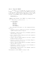
Sensing modules:
• Mice: a dead reckoning sensor for indoor mobile robotics, it supports
reliable odometry using a set of optical mice connected to the robot
body as in Figure 12.5;
• RecVision: [?] todo...
• MUREA: the localization module, its aim is to estimate the robot pose
with respect to a global reference frame from sensor data, using a map
of the environment;
• MAP : the world modelling module, it builds and keeps a representation of the external world inside the intelligence of the robot, integrating the information gathered through its sensors;
Acting module:
• AirBoard : description...
Reasoning modules:
• MrBRIAN : the controlling module, it manages all the primitive actions, typically implemented as reactive behaviors, that can be executed by the robot;
• SPIKE : the trajectory planning module based on the geometric map
of the environment, this module selects a proper path from a starting
position to the requested goal;
• SCARE : the coordination and sequencing module, it allows robots to
share perceptions and to communicate intentions in order to perform
effective task allocation, this module is also responsible for the execution of a given plan, monitor its progress, and handling exceptions as
they arise.
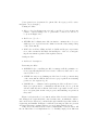
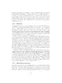
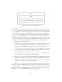
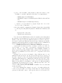
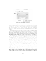
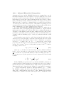
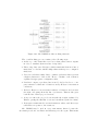
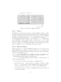
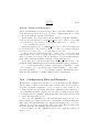
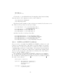
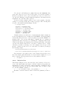
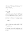
Figure 2.4 depicts the robotic functional modules described in this manual, arranged in a typical hybrid control architecture, in which the deliberative and reactive layers are combined through a middle layer that realize a
sequencing mechanism. In Figure 2.4 all the reasoning modules are present
and typical message passing path are reported using dashed arrows.
A key factor in software reuse is the configurability of the modules. All
the modules have been implemented to be usefully employed in different
9
The Modular Robotics Toolkit
Localization
-- MUREA --
Planning
-- SPIKE --
Coordination
& Sequencing
-- SCARE --
World
Modelling
-- MAP --
Controlling
-- MrBRIAN --
Sensors
Modules
Actuator
Modules
Communication
with other robots
or human users
Network
Interface
Environment, Other Robots and User
Figure 2.1: The general architecture implemented by the MTR
applications besides RoboCup, as described in [9]. For this reasons, each
module requires some configuration files to define those parameters that are
application specific. In the following chapters, each module will be presented
along with same examples of configuration files.
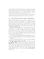
2.2
Middleware for Modules Integration
Having different modules that cooperate to obtain a complex control architecture requires a flexible distributed approach. At the same time, autonomous robotic systems, particularly those involving multiple robots and
environmental sensors, such as RoboCup, are becoming increasingly distributed and networked. For this reasons, a distributed, concurrent and
modular middleware to support integration and communication is required.
The DCDT middleware supports a publish/subscribe architectures hiding the physical distribution of the modules. In this model, data providers
publish data and consumers subscribe to the information they require, receiving updates from the providers as soon as this information has been
published.
This paradigm is based on the notion of event or message. Components
interested in some class of events subscribe expressing their interests. Components providing information publish it to the rest of the system as event
notification. This model introduces a decoupling between producers and
10
subscribers through the fact that publishers and subscribers do not know
each others.
This model offers significant advantages essentially to time-changing values of an otherwise continuous signal, such as the senses data and the control
signals of the robots of the Milan RoboCup Team. For further details about
the advantages of a publish/subscribe architecture compared to other strategies, take a look at [9]. Next chapter will focus on DCDT, the middleware
that makes possible the interaction and the communication between all the
modules in the MRT architecture.
2.3
Applications
[—valutare se mettere in questo paragrafo una descrizione del flusso di informazione tra i vari moduli: es: dal modulo mice si hanno dei dati che vanno
in ingresso al modulo brian (per assurdo) e anche al modulo MUREA i cui
output, ecc ecc, facendo riferimento alla figura con il flusso tra i moduli in
questo capitolo————————-]
The MRT framework has been used to develop robotic applications with
different robot platforms and in a few contexts. The general structure of
the Modular Robotics Toolkit is reported in Figure 2.4 including all the
implemented modules and the typical message passing connections between
them.
Since different platforms have been used, from custom bases with differential drive or omnidirectional wheels to commercial all-terrain platforms,
the use of a proper abstraction layer in sensing and actuation modules allowed us to focus mainly on the development of robot intelligence.
Typical user might not need all of the modules implemented in MRT so it
is possible to select the subset that suits the needs of the specific application.
In the following, three different architectures will be presented. They are
three case studies where MRT was successfully used to reduce in a sensible
way the “time to market” for the requested application.
2.3.1
Roby
Roby is a project part of the framework of the European project GALILEO.
It has been developed in collaboration with the Italian company InfoSolution. In this project, a robot, equipped with a Differential GPS device, must
travel between two points, chosen over a pre-compiled map of an outdoor
environment. An external path planner computes the sequence of points
which describe a free path and sends the set of way points to the robot
through a wireless connection.
The map of the external planner contains only information about static
objects such as buildings, bridges, etc.; for this reason, the robot is also
11
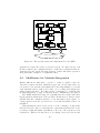
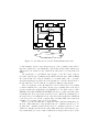
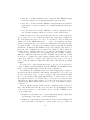
Roby
Localization
-- MUREA --
Planning
-- SPIKE --
Sequencing
-- SCARE --
World
Modelling
-- MAP --
Communication
with remote user
Controlling
-- MrBRIAN --
Encoders
Sonar belt
DGPS
ActiveMedia
P3-AT Control
Wireless
Network
Outdoor Environment and
External Planner
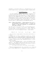
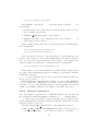
Figure 2.2: MRT modules involved in the Roby case study
equipped with a sonar belt in order to detect obstacles, so that it can handle situations in which the trajectory produced by the planner is obstructed
by something, for example cars, trees, people, etc. The robot used in this
application is an ActiveMedia P3-AT platform with a differential drive kinematics.
In Figure 2.2 you can see the architecture of the Roby case study. Only
few modules are used since the planner is external and it is simply requested
a path-following behavior. No complex world modelling is needed since the
Differential GPS provides already a good estimation of robot position and
this is sufficient to accomplish the task. Even if this is a single robot domain,
the coordination level, implemented in SCARE, has been used in order to
allow Mr-BRIAN to follow the sequence of path-points with a simple reactive
behavior.
Each task ReachPathPoint terminates when either the robot reaches the
related path point (success condition), or a timeout expires (failure condition). In the former case, the current task ends, and the ReachPathPoint
task related to the next path point is activated. In the latter case, the whole
task is aborted, and the planning module is requested to produce, starting
from the current robot position, a new sequence of path points.
During navigation, data collected from the sonar belt are used directly
by the behavior engine in the reactive AvoidObstacle behavior, since we
want our robot to promptly react in avoiding collisions. Although the im12
plemented structure is very simple, we have obtained satisfactory results in
several trials with different conditions, and the robot was always able to
reach the goal point dealing with unforeseen obstacles. The wireless connection has been also used by a person to drive the robot in a tele-operated
fashion while keeping active sensing modules to implement safety obstacle
avoidance. You can see some sample movies on the real robot on the InfoSolution web site [1].
2.3.2
FollowMe
FollowMe is a project to develop a guide robot to be deployed at the Science
and Technology museum in Milan. In this case, the task to be accomplished
is more complex with respect to Roby: the robot has to guide a visitor in
the museum, whenever the visitor stops next to an exhibit, it has to wait
and move again on the tour as the visitor starts moving again. Sometimes
it may happen that the visitor moves away attracted by some interesting
piece and in this case the robot has to follow him, re-plan the tour and start
again the visit as soon as the visitor is ready.
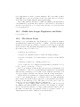
The robot used in this indoor application has a differential drive kinematics with shaft encoders and it is provided with an omnidirectional vision
system able to detect obstacles as well as landmarks in the environment.
Not having a reliable positioning sensor like the Differential GPS, this application requires a more complex set-up for the localization module that
has to fuse sensor information and proposed actuation to get a reliable positioning. MUREA has thus a twofold role in this application: sensor fusion
and self localization. Information coming from different sources is fused by
using the framework of evidence and the robot position is estimated as the
pose that accumulate the most evidence.
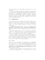
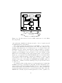
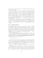
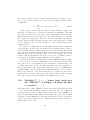
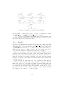
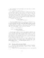
Figure 2.3 describes the MRT modules involved in the FollowMe application. In this case the architecture includes also the trajectory planner
SPIKE triggered by the sequencing module SCARE whenever a new tour
is required. Almost any behavior used in MR-BRIAN and job in SCARE
for the Roby application have been reused, as the message containing points
generated by the planner is equivalent to the message transmitted through
the wireless network in that application. This time the coordination is limited to the interface with the user while acquiring the characteristics of the
tour, such as destination, object of interests and so on.
2.3.3
Milan RoboCup Team
The third case study shows how MRT has been successfully applied in the
RoboCup competition, where autonomous robots play soccer in a domain
with both cooperative and adversarial aspects. In this section only a brief
description will be presented, since this application will be the case study
13
FollowMe
Localization
-- MUREA --
Planning
-- SPIKE --
Coordination
-- SCARE --
World
Modelling
-- MAP --
Communication
with human user
Controlling
-- MrBRIAN --
Encoders
Omni-Vision
Custom
Differential
Drive Control
Wireless
Network
Environment and User
Figure 2.3: Modules involved in the FollowMe architecture
of this manual. In the next chapters most of the examples that will be
introduced will refer to the Milan RoboCup Team. Besides that, Chapter 12
will describe in detail how the different modules have been integrated in
MRT.
We participate to the Middle Size League of the RoboCup competition since 1998 at the beginning in the ART team and since 2001 as Milan
RoboCup Team. RoboCup is a multi-robot domain with both cooperative
and adversarial aspects, and it is perfectly suited to test the effectiveness of
the Modular Robotics Toolkit in a completely different environment.
The development of the Modular Robotics Toolkit followed a parallel
evolution with the Robocup Team. At the very beginning there was only a
reactive architecture implemented by BRIAN (i.e., the first version of MrBRIAN), after that SCARE and MUREA followed to realize an architecture
resembling the Roby case study presented before. While the planning module was developed to fullfil the needs of the FollowMe application, MAP has
been developed to model the complex task of dealing with sensor fusion in
a multy-robot scenario and opponed modelling.
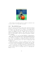
The robots used in this indoor application have different kinematics; we
used two differential drive custom platforms, two omnidirectional robot exploiting three omnidirectional wheels and one omnidirectional robot base
with four omnidirectional wheels. Only differential drive platforms are provided with shaft encoders so that localization is entirely vision based on the
14
Milan Robocup Team
Localization
-- MUREA --
Planning
-- SPIKE --
Coordination
& Sequencing
-- SCARE --
World
Modelling
-- MAP --
Controlling
-- MrBRIAN --
Encoders
Omnivision
Custom
Omnidir
Control
Communication
with teammates,
monitor or referees
Wireless
Network
Environment, Teammates,
Monitor and Referees
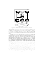
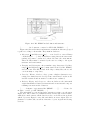
Figure 2.4: Modules involved in the MRT architecture for the Milan
RoboCup Team
other platforms. Omnidirectional vision is used to detect obstacles as well
as landmarks in the environment.
The software architecture implemented with MRT to be used in these
robots is quite different from the previous ones. Since RoboCup is a very
dynamic environment the robot behaviors need to be mostly reactive and
planning is not used. On the other hand, RoboCup is a multi-robot application and coordination is needed to exploit an effective team play. From the
schema reported in Figure 2.4 it is possible to notice the central role that
MAP, the world modelling module, plays in this scenario. Sensor measurements (i.e., perceptions about visual landmarks and encoders when available) are fused with information coming from teammates to build a robust
representation of the world. This sensor fusion provide a stable, enriched
and up-to-date source of information for MrBRIAN and SCARE so that controlling and coordination can take advantage from perceptions and believes
of other robots.
Coordination plays an important role in this application domain thus
SCARE is used more extensively for this task. We have implemented several jobs (RecoverWanderingBall, BringBall, Defense, etc.) and schemata
(DefensiveDoubling, PassageToMate, Blocking, etc.). These activities are
executed through the interactions of several behavioral modules. Also MrBRIAN has been fully exploited in this application; we have organized our
15
behaviors (i.e., basically macro actions) in a complex hierarchy. At the first
level we have put those behavioral modules whose activation is determined
also by the information coming from the coordination module. At this level
we find both purely reactive modules and parametric modules (i.e., modules that use coordination information introduced in MAP by SCARE). The
higher levels contain only purely reactive behavioral modules, whose aim is
to manage critical situations (e.g., avoiding collisions, or leaving the area
after a timeout). For more details about the different modules implemented
in MRT refer to the following chapters, and in particular see Chapter 12
for a detailed discussion about how MRT has been applied in the RoboCup
competition.
16
Chapter 3
Device Communities
Development Toolkit
DCDT, Device Communities Development Toolkit, is the framework used to
integrate all the modules in MRT. This middleware has been implemented
to simplify the development of applications where different tasks run simultaneously and need to exchange messages. DCDT is a publish/subscribe framework able to exploit different physical communication means in
a transparent and easy way.
The use of this toolkit helps the user dealing with processes and inter
process communication, since it makes the interaction between the processes
transparent with respect to their allocation. This means that the user does
not have to take care whether the processes run on the same machine or on
a distributed environment.
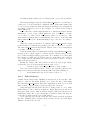
DCDT is a multi-threaded architecture consisting in a main active object, called Agora, hosting and managing various software modules, called
Members. Members are basically concurrent programs/threads executed periodically or on the notification of an event. Each Member of the Agora can
exchange messages with other Members of the same Agora or with other
Agoras on different machines.
The peculiar attitude of DCDT toward different physical communication
channels, such as RS-232 serial connections, USB, Ethernet or IEEE 802.11b,
is one of the main characteristics of this publish/subscribe middleware.
3.1
Agora and Members
An Agora is a process composed of more threads and data structures required to manage processes and messages. Each single thread, called Member in the DCDT terminology, is responsible for the execution of an instance
of an object derived from the DCDT Member class.
It is possible to realize distributed applications running different Agoras
17
Figure 3.1: Structure of the Agora
on different devices/machines, each of them hosting many Members. It is
also possible to have on the same machine more than one Agora that hosts
its own Members. In this way you can emulate the presence of different
robots without the need of actually having them connected and running.
There are two different type of Members, User Members and System
Members. The main difference between the two is that System Members are
responsible for the management of the infrastructure of the data structures
of the Agora, while User Members are implemented by the user according
to his needs. Moreover System Member are invisible to User Members.
The main System Members are:
• Finder : it is responsible for searching for other Agoras on local and
remote machines dynamically with short messages via multicast;
• MsgManager : this Member manages all the messages that are exchanged along several members. In case each single Member handles
its own message queue locally, the MsgManager takes care of moving
messages from the main queue to the correct one;
• InnerLinkManager : its role is to arrange inter Agora communication
in case they are executed on the same machine;
• Link : those Members handle communication channels between two
Agoras, so that they messages can be exchanged. Each link is responsible for the communication flow in one direction, so there are separate
Members for message receiving and sending;
Members of the Agora can exchange messages through the PostOffice,
using a typical a publish/subscribe approach. Each Member can subscribe
to the PostOffice of its Agora for a specific type of messages. Whenever a
Member wants to publish a message, it has to notify the PostOffice, without
taking into accont the final destinations of the deliveries.
18
3.2
Messages
DCDT Messages are characterized by header and payload fields. The header
contains the unique identifier of the message type, the size of the data contained in the payload and some information regarding the producer.
Members use unique identification types to subscribe and unsubscribe
messages available throughout the community. Messages can be shared basically according to three modalities: without any guaranty (e.g. UDP),
with some retransmissions (e.g. UDP retransmitted), with absolute receipt
guaranty (e.g. TCP).
Sometimes the payload of a Message can be empty. For example you
can use Messages to notify events, in this case the only information is the
specific event that matches a particular Message type. This implies that all
the Agoras must share the same list of Message types.
In MRT, the interfaces among different modules are realized through
messages. According to the publish/subscribe paradigm, each module may
produce messages that are received by those modules that have expressed
interest in them. In order to grant independence among modules, each module knows neither which modules will receive its messages nor the senders
of the messages it has requested. In fact, typically, it does not matter which
module has produced an information, since modules are interested in the
information itself.
For instance, the localization module may benefit from knowing that
in front of the robot there is a wall at the distance of 2.4 m, but it is
not relevant which sensors has perceived this information or whether this
is coming from another robot. For this reason, our modules communicate
through XML (eXtensible Markup Language) messages whose structure is
defined by a shared DTD (Document Type Definitions). Each message
contains some general information, such as the time-stamp, and a list of
objects characterized by a name and its membership class.
For each object may be defined a number of attributes, that are tuples
of name, value, variability, and reliability. In order to correctly parse the
content of the messages, modules share a common ontology that defines the
semantic of the used symbols.
The advantages of using XML messages, instead of messages in a binary
format, are: the possibility of being readable by humans and of being edited
by any text editor, well-structured by the use of DTDs, easy to change and
extend, the existence of standard modules for the syntactic parsing. These
advantages are paid by an increase in the amount of transferred data, parsing
may need more time, binary data can not be included directly.
The middleware encapsulates all the functionalities to handle Members
and Messages in the Agora, so that the user does not have to take care of
executing each single thread neither handling message delivery. This results
in making the use of this middleware very easy.
19
3.3
Configuration Files and Examples
The Agora is the main object instantiated in every application that makes
use of DCDT. Each Agora is composed of threads, called Members, that
execute specific tasks and communicate through messages.
The Agora can be instantiated using two different options called STANDALONE and NETWORK, according to the physical distribution of the
Members. If you want Members to exchange messages from different machines, you need to use the NETWORK option, otherwise you can use the
STANDALONE. Both allow the communication along Members of the same
Agora and between Agoras on the same machine.
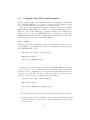
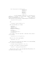
3.3.1
Agora
Different Agoras can communicate on the same machine through local sockets, this simple code fragment shows how you can instantiate an Agora using
the STANDALONE option.
int main (int argc, char *argv[]) {
DCDT_Agora *agora;
agora = new DCDT_Agora();
....
}
Otherwise you can create an Agora using the NETWORK option. In this
case you need to write a configuration file with all the network parameters
required to allow communication between the different machines where the
Agoras are executed. The following code lines show the use of the overloaded
constructor that takes the configuration file as parameter.
int main (int argc, char *argv[]) {
DCDT_Agora *agora;
agora = new DCDT_Agora("dcdt.cfg");
....
}
The configuration file for the Agora includes the following information:
• network parameters of the machine: these parameters define the TCP/IP
address and the port of the Agora, plus the multicast address of the
local network;
20
• policy of the PostOffice: this parameter define the behavior of the
PostOffice, so far three different policies have been implemented:
– SLWB: Single Lock With Buffer;
– SLWDWCV: Single Lock With Dispatcher With Conditional Variable;
– SLWSM: Single Lock With Single Message;
[—-Queste voci sopra andrebbero spiegate meglio ma c’ da cercare
dove sono state documentate——-]
• list of the available communication channels: this is a list of static links
to other Agoras, using different physical communication channels, such
as:
– RS-232 serial connections;
– TCP/IP network addresses
You can use the DCDT framework also in dynamic environment when
the addresses of the machines are not known a priori, in this case the Finder
Member of the Agora can use the multicast address to search for other Agoras on the local network. When the Agoras belong to different networks the
multicast address and the Finder are useless. In this case the communication
involves directly the Members, as it will be described below.
[——-INIZIO parte da rivedere (continua fino a FINE parte da rivedere)—
—– questa parte va rivista a tavolino con matteo, perch ci ono delle cose
che non vanno. es: non chiaro cosa si intende con memeberche che iteragiscono ”directly”. vanno spiegati meglio i thread LinkRx e LinkTx. va
spieato meglio la differenza tra link e bridge. quando si dice the tutti i messaggi vengono transmitted, non viene detto dove. e la questione del level va
chiarita.——–]
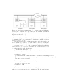
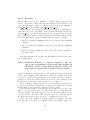
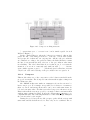
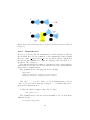
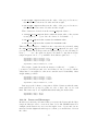
In Figure 3.2 you can see an example of three different types of communications among Agoras. Agora1, Agora2 and Agora3 are executed on
the same computer, so they can exchange messages through the InnerLinkerManager that handles the communication when the Agoras reside on the
same machine; Agoras1 and Agora4 belong to the same network and the
Finder is responsible for searching for other Agoras on different machines
dynamically; Agora4 and Agora5 belong to different networks, so the communication involves the Members directly.
[——– che cosa sono i moduli LinkRx e LinkTx? Non sono mai stati
menzionati prima...——-]
For each communication channel, you need to determine whether the
local node acts as a link or as a bridge. In the first case only the messages
generated locally will be sent to other Agoras, in the second case the node
21
Figure 3.2: Inter Agora communication. [——–questa figura probabilmente
non va bene... mancano dei componenti forse, tipo LinkTX e LinkRx in
Agora1. Inoltre le Agora vanno scritte con il numero attaccato al nome, es
Agora1 e non Agora 1——-]
will work as a bridge, and all the messages, both received an generated, will
be transmitted. A proper configuration of the channels as links or bridges
grants the absence of loops.
If the Agoras are executed on different machines on a local network, you
need to list all the IP address. For each channel, you need to identify the
local and remote IP address, the local and remote port, and the level. [—
——cos’ questo level?———–]. If the communication channel is a RS-232
serial connection, you only need to determine the level and the device used
to exchange messages with other Agoras.
[——-FINE parte da rivedere——–]
This is the complete template for the configuration file of the Agora:
<local IP addr> <multicast addr> <port>
PostOffice: <type>
[---controllare il formato del file: dove metto link|bridge???????]
[ip <mod> <lev> <local addr> <local port> <remote addr> <remote port>]*
[ser <mod> <lev> <device>]*
This an example of a specific instance of an Agora:
192.168.0.1 225.0.0.1 2003
PostOffice: SLWB
ip link 0 192.168.0.1 3000 192.168.1.1 3000
The first line states that the local network IP address of the machine
where the Agora is executed is set to 192.168.0.1. The Agora is listening
22
on port 2003, and the multicast address is 225.0.0.1. The PostOffice, it has
been implemented using a Single Lock With Buffer policy. The last line
states that the local Agora is connected with a remote machine through a
TCP/IP network. The remote host has the IP address set to 192.168.1.1,
both local and remote Agoras use port 3000.
Since you can run more than one Agora on the same machine and considering that the Agora allocation is completely transparent with respect the
physical distribution, you can easily test a system locally and then switch
from STANDALONE to NETWORK to test a distributed environment.
3.3.2
Members
You can easily add a Member to an Agora, using the method AddMember(Member
member). This action causes the creation of the data structures responsible
for the management of the Member inside the Agora. When you want to
activate the Member, you have to call the method ActivateMember(Member
member). As a consequence the thread that will execute the Member will be
created. This simple example shows how to add an instance of MemberZero
to the Agora.
int main(int argc, char **argv) {
DCDT_Agora *agora;
MemberZero *member0;
agora = new DCDT_Agora("dcdt.conf");
member0 = new MemberZero(agora);
agora->AddMember(member0);
agora->ActivateMember(member0);
.....
}
Using the method LetsWork() you can start the execution of all the
active Members of the Agora. The call is synchronous and will return when
the Agora will be terminated. This happens when all the Members of the
Agora are in the TERMINATING state, or when one of the Members call
the method Shutdown(). This causes the the Agora to terminate all the
Members within the current activity cycle.
The User Members are implemented by the user to accomplish specific
tasks. According to the DCDT architecture the Members are executed in
parallel and each Member corresponds to a particular thread. In this way
all the Members can share the same variables, this allows the exchange of
messages between all the participants of the Agora.
23
There are two different kind of Members:
• Periodic Execution Members: in this kind of Members the method
DoYourJob() is executed periodically, and the period is set by the
user when the Member is initialized;
• Cyclic Execution Members: in this case the method DoYourJob() is
called cyclically without delay.
The following example show how you can implement a Periodic Execution Member. The constructor of the DCDT Member class takes two
parameters, the Agora and the number of milliseconds of the period. If you
want to create a Cyclic Execution Member you have to drop the second
parameter of the constructor of the base class. As you can see, each instance of a Member must implement the class DCDT Members or one of its
subclasses.
class MemberZero : public DCDT_Member {
public:
MemberZero (DCDT_Agora*);
MemberZero();
void Init();
void Close();
void DoYourJob(int);
};
MemberZero::MemberZero (DCDT_Agora* agora)
:DCDT_Member(agora,20000){};
Actually, you can create a third kind of Member, combining Messages
and Members, for example you can create a Member that is executed whenever a particular type of Message is received. You can accomplish this behavior subscribing for a particular type of message inside the method Init()
of a Member.
[———questo esempio appena menzionato andrebbe presentato per esteso—
—]
Each Member can subscribe for a specific type of Message using the
following method:
void SubscribeMsgType(int type,
DCDT_RequestType ReqType=DCDT_ALL_MSG)
24
The second parameter of the method allows to set the request type. If
it is set to DCDT LOCAL MSG, the Member will receive only the Message sent from local Agoras or from Agoras linked though a channel set to
BRIDGE. Using the DCDT REMOTE MSG request type, the Member will
receive only the Messages sent from Member belonging to Agoras linked using a LINK channel. Otherwise, if the parameter is set to DCDT ALL MSG,
all Messages will be received.
You can either unsubscribe from a particular Message type:
void UnSubscribeMsgType(int type,
DCDT_RequestType ReqType=DCDT_ALL_MSG)
or unsubscribe from all the Messages:
void UnSubscribeAll()
Each Member can create a Messages using these methods:
DCDT_Msg* CreateMsg(int type, int delivery_warranty)
DCDT_Msg* CreateMsg(int type)
The current Message can be removed form the Message queue with
void RemoveCurrMsg()
The destructor will be invoked unless other Members are waiting to
receive the Message. Members can send Messages to the PostOffice using
the method:
void ShareMsg(DCDT_Msg *msg)
Thanks to the PostOffice, that handles the queue of Messages, the Message will be delivered to all the Agoras that contain Members that subscribed
to a particular Message type.
Members can receive Messages they subscribed for using the method:
DCDT_Msg* ReceiveMsg(void)
To learn more about how to handle Agoras and Members, take a look at
[15] for the DCDT User Manual.
25
3.3.3
Messages
Messages in the DCDT middleware are composed of two parts:
• Header : it includes all the information about the message such as:
– Type: a number that identifies unequivocally the type of Message;
– MemberID: a number that identifies the Member that created the
Message
– AgoraID: a number that identifies the Agora where the Message
has been created;
– Priority: the priority of the Message (not yet supported);
– Delivery warranty: the warranty that the Message has been sent
though the channel (not yet supported).
• Payload : the body of the message, it contains the data exchanged
among the Members. There is no marshaling policy, so the user has
to handle complex data structures to ensure that they are allocated in
contiguous memory areas.
Each Message has some methods that allow the user to get some information about the Message itself. For example you can get the Agora ID
using:
int ReadAgoraID()
The following method returns the Payload of the Message:
void *GetPayload()
You can also know when the Message has been create using:
DCDT_TIME ReadCreationTime()
Finally you can get the size of the Payload of the Message with:
int ReadPayloadLen()
This chapter aimed to introduce the toolkit, for a comprehensive guide
to DCDT, see the User Manual [15] and the ..........
[———-esiste della documentazione sul codice di DCDT (tipo javadoc?)—
] [———-rimangono fuori i dettagli sul PostOffice———-]
26
Chapter 4
Mice
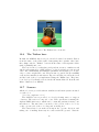
Some of the robots developed withing the AIRLab, for example the IANUS3
base for the robots of Milan RoboCup Team, are provided with a dead reckoning sensor in order to support reliable odometry. The sensor is composed
of two optical mice to estimate the robot pose. Refer to Chapter 12 for some
pictures of the robot base.
Dead reckoning is a navigation method based on measurements of distance traveled from a known point used to incrementally update the robot
pose. This leads to a relative positioning method, which is simple, cheap and
easy to accomplish in real-time. The main disadvantage of dead reckoning
is its unbounded accumulation of errors.
The majority of mobile robots use dead reckoning based on wheels velocity in order to perform their navigation tasks. Typically odometry relies on
measures of the space covered by the wheels gathered by encoders which can
be placed directly on the wheels or on the engine-axis, and then combined in
order to compute robot movement along the x and y coordinates of a global
frame of reference and its change in orientation.
It is well-known that this approach to odometry is subject to errors
caused by factors such as unequal wheel-diameters, imprecisely measured
wheel diameters or wheel distance, irregularities of the floor, bumps, cracks
or by wheel-slippage.
The localization system used for the robots is based on the measures
taken by two optical mice fixed on the bottom of the robots as you can see
in Figure 12.5. Such sensor is very robust towards non-systematic errors,
and independent from robots kinematics, since it is not coupled with the
driving wheels and it measures the effective robot displacement.
Furthermore, this is a very low-cost system which can be easily interfaced with any platform, thus can be used to integrate standard odometry
methods. In fact, it requires only two optical mice which can be placed in
any position under the robot, and can be connected using the USB interface.
One of the problems of this sensor, is that it can be used only in an
27
environment with a ground that allows the mice to measure the movements.
As to RoboCup, where the sensors is extensively used, usually the fields meet
this requirement. In fact, the only issue by using this method is related to
excessive missing readings due to a floor with a bad surface or when the
distance between the mouse and the ground becomes too large.
In the next sections, the sensor will we briefly introduced, you will see
the main aspects of geometrical derivation that allows to compute the robot
movement, along with a simple procedure to perform error detection.
4.1
The Odometry Sensor and Pose Estimation
From the readings of the two mice it is possible to compute the pose of a
mobile robot independently from its kinematics. For example, let us suppose
that the mice are placed at a certain distance D, so that they are parallel
between them and orthogonal with respect to their joining line. Consider
their mid-point as the position of the robot and their direction, for example
their longitudinal axis pointing toward their buttons, as its orientation. This
initial hypothesis simplifies many of the following considerations, but it can
be easily relaxed as shown in [8].
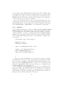
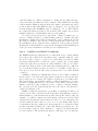
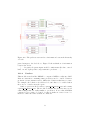
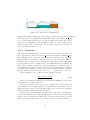
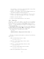
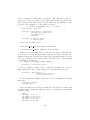
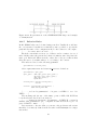
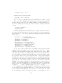
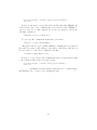
Each mouse measures its movement along its horizontal and vertical
axes. Whenever the robot makes an arc of circumference, also each mouse
will make an arc of circumference, which are characterized by the same
center and the same arc angle, but different radius. During the sampling
time, the angle α between the x-axis of the mouse and the tangent to its
trajectory does not change. This implies that, when a mouse moves along
an arc of length l, it measures always the same values independently from
the radius of the arc, as in Figure 4.1.
You can easily assume that, during the short sampling period, the robot
moves with constant tangential and rotational speeds. This implies that the
robot movement during a sampling period can be approximated by an arc
of circumference.
Given the 4 readings taken from the two mice, the arc of circumference
can be described using 3 parameters, the x and y coordinates of the center
of instantaneous rotation and the rotation angle.
We call xr and y r the measures taken by the mouse on the right, while
xl and y l are those taken by the mouse on the left. Notice that the are only
3 independent data; in fact, there’s the the constraint that the respective
position of the two mice cannot change. This means that the mice should
read always the same displacement along the line that joins the centers of
the two sensors. In particular, if the mice are placed as in Figure 4.1, the
x values measured by the two mice should be always equal: xr = xl . This
redundancy will be used for error detection and reduction in case of wrong
measurements.
28
Figure 4.1: The angle arc of each mouse is equal to the change in orientation
of the robot [—–forse angle arc non va bene, ma la stessa didascalia che c’
in un articolo di Bonarini e Restelli e Matteucci, A kinematic-independent
dead-reckoning sensor...—-]
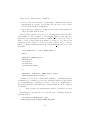
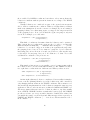
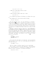
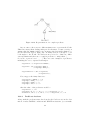
Figure 4.2: The triangle made up of joining lines and two radii
29
You can compute how much the robot pose has changed in terms of ∆x,
∆y, and ∆θ. In order to compute the orientation variation ∆θ you can
apply the cosine rule to the triangle made by the joining line between the
two mice and the two radii between the mice and the center of their arcs,
as in Figure 4.2:
D2 = rr2 + rl2 − 2 cos(γ)rr rl ,
(4.1)
where rr and rl are the radii related to the arc of circumferences described
respectively by the mouse on the right and the mouse on the left, while γ
is the angle between rr and rl . It is easy to show that γ can be computed
by the absolute value of the difference between αr and αl , where αi is the
angle between the x-axis of the ith mouse and the tangent to its trajectory.
The radius r of an arc of circumference can be computed by the ratio
between the arc length l and the arc angle θ. In this case, the two mice are
associated to arcs under the same angle, which corresponds to the change
in the orientation made by the robot.
With simple substitutions, you can get the following expression for the
orientation variation:
q
rl2 + rr2 − 2 cos(γ)lr ll
· sign(y r − y l )
(4.2)
D
The movement along the x and y axes can be derived by considering
the new positions reached by the mice with respect to the reference system
centered in the old robot position, and then computing the coordinates of
their mid-point.
From the mice positions, you can compute the movement executed by
the robot during the sampling time with respect to the reference system
centered in the old pose.
The absolute coordinates of the robot at time t + 1 (Xt+1 , Yt+1 , Θt+1 )
can thus be computed by knowing the absolute coordinates at time t and
the relative movement carried out during the period (t; t + 1] (∆x, ∆y, ∆θ)
through these equations:
∆θ =
Xt+1 = Xt +
Yt+1 = Yt +
q
∆x2 + ∆y 2 + cos Θt + arctan
q
∆x2 + ∆y 2 + sin Θt + arctan
∆y
∆x
∆y
∆x
Θt+1 = Θt + ∆θ
More details about the expressions above can be found in [6].
30
(4.3)
(4.4)
(4.5)
4.2
Sensor Error Detection and Reduction
Odometry is affected by two kind of errors: systematic and non-systematic.
The systematic errors that can affect this odometric sensor are:
• imperfections in the measurements of the positions and orientations of
the two mice with respect to the robot;
• the resolution of the mouse, which depends from the surface on which
the robot must travel;
• different resolutions of the two mice.
Most of these systematic errors can be corrected through calibration.
The odometric system needs to know the value of some parameters related
to the positioning of the two mice: the distance between the two mice D,
the orientation σr and σl with respect to the robot heading, and the angle δ
between the robot heading and the direction orthogonal to the mice joining
line. If these parameters are not correctly estimated, systematic errors will
be introduced. In order to identify the parameters of the odometric sensor,
you need to perform the calibration procedure described in [8].
The calibration procedure consistes in two practical measurements: the
translational measurement and the rotational measurement. The translational measurement consists in making the robot travel (manually) 500 mm
forward for ten times, and, for each time, storing the mice readings. At the
end of the measurement the averages of the four readings can be computed,
which allows to estimate the mice resolutions and the angle between the
robot and the mouse heading.
In the rotational measurement the mice readings are taken after a counterclockwise 360◦ revolution that the robot makes around its rotational axis;
this process is repeated five times. The averages of these readings allow
to estimate the distances between the center of rotation and the two mice,
the angle between the mouse heading and the tangential to the circumference described during the revolution, and the distance between the two mice
projected to the x and y-axes.
As to non systematic errors, there are two main sources of errors:
• slipping: it occurs when the encoders measure a movement which is
larger the the actually performed one, such as when the wheels lose
the grip with the ground;
• crawling: it is related to a robot movement that is not measured by
the encoders, for example when the robot is pushed by an external
force.
They can be reduced considering that the parameters required for estimating the robot pose, according to the initial hypotheses, are 3 and the
31
two mice give 4 readings, the redundancy of the input data can exploited
in order to detect if they are consistent with the model. This can be used
to detect non-systematic errors in mice readings due to uneven surface or
homogeneous areas. To detect such errors, you can use the constraint that
the distance between the two mice has to be constant.
If the equality of is not verified it means that one or more of the mice
readings are erroneous. On the other hand, if the constraint is verified you
cannot assert that the input data are correct, but only that they satisfy the
model.
Since there is only one constraint, once we detect an error, you cannot
know which of the four measures are wrong. Nevertheless, if you make some
hypotheses on the kind of errors which affect the mice readings, the error
can be reduced.
In general, a measure is never greater than the movement actually performed by the mouse, the reason for this is that, typically, the errors made by
an optical mouse are caused by a change in the distance between the mouse
and the ground or by a surface which is homogeneous. In these cases, it can
happen that during the sampling time t the mouse does not perceive the
actual movement for a time t0 ≤ t.
Due to the hypothesis that during the sampling time the translational
and rotational velocities of the robot are constant, it follows that also the
velocities of the mouse along its axes are constant. This implies that the
errors affect only the measure of the length of the path covered by the mice
(lr and ll ), and not the angle with which they travel along their trajectory
(αr and αl ). In this way, the number of variables has been decreased from
4 to 2.
If at least one mouse is not affected by errors, the errors of the other
mouse can be corrected, otherwise you can only reduce the erroneous readings of one mouse.
4.3
TODO Configuration Files and Examples
TODO
32
Chapter 5
AIRBoard
[—————-in tutto il manuale c’ da controllare le voci degli indici e uniformare il posto in cui vengono fatte le citazioni agli articoli————-]
The main acting module developed within the MRT framework is called
AIRBoard. This unit is responsible to control a set of actuators for many
of the robots designed within the AIRLab, both those with omnidirectional
wheels and the ones with differential drive. The actuators of the robots
are the motors directly connected to the wheels of the platform. As you
learned in Chapter 2, each acting module can be divided into two parts,
the drivers sub-module that directly interacts with the physical device, and
the processing sub-module that is interfaced on one side with a driver submodule, and on the other with some reasoning modules. [—sto dicendo
una cosa corretta nella frase che segue?———-] Before going through the
description of the architecture, notice that AIRBoard is not only the name
of the module, but also the name of the printed circuit boards that hosts the
embedded system for the low-level control of the motors. In this case the
physical device cannot be directly connected to the personal computer as
with USB or firewire peripherals, an electronic circuit to control the motors.
[———–qui metterei una figura in cui mostrare come hardware il collegamento PC-scheda-motori e come software il modulo associato al PC e il
systema embedded asociato alla scheda——–]
Figure ?? shows.... [———in base alla figura segue una descrizione
dell’immagine.——–]
In this chapter you will learn about the design choices underneath the
AIRBoard, including both the module and the embedded system developed
on the board, and how it can be used to send set points to the different
actuators.
33
5.1
Hardware and Sotfware Design
In the first part of this section you will learn about the electronic board
that makes possible for the AIRBoard module to control the motors of the
robots. The PCB can be logically and physically divided into two parts, the
digital circuit that handles the communication with the PC and interprets
the commands coming from the bus, and the analog power circuit that
directly drives the motors [——-forse quest’ultimo punto si pu sistemare
meglio———-].
[———-Figura di uno schema a blocchi concettuale della scheda———–
digital microcontroller, analog power circuit, encoders, serial line interface,
ecc ecc———–] [———-Domanda: con ’sistema embedded’ si intende sola
una parte della scheda, quella che gestisce la logica di controllo, o tutta la
scheda, compresa la parte di potenza?———–]
Figure ?? shows the block the board is make of, and how they are connected to each other.
[———-Segue descrizione dei macroblocchi della scheda———–Ad esempio per il microcontrollore: considered embedded system, its core is a
microcontroller that has been programmed to perform a specific task. As
you will see the firmware, the software of the microcontroller, handles the.....]
Pulse Width Modulation (PWM) is a common and simple way for interfacing digital and analog devices. Since in AIRboard the control logic is
programmed with a digital microcontroller and the DC motor is driven by
an analog power circuit, we use PWM to connect them
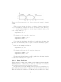
A PWM signal is a periodic signal made up of pulses with a variable
width. Period and duty cicle that is the width of the pulses in time units
are the characteristic parameters of such a signal (see figure 1.1). Period is
fixed during the operation of the system and the main considerations that
must be addressed regarding its choice are: Audible frequency band: the
PWM frequency must be outside the audible frequency band, otherwise a
disturbing noise would be heard.
Compatibility with analog circuits: the PWM frequency must be chosen
so that analog circuits (that will receive that signal as input) would be able
to process it.
The board consists of a PIC (PIC18F252) -
5.2
The board
Since the oscillator frequency is correlated with the clock frequency according to the following formula: Fclock = 1 4Fosc we have chosen the maximum
oscillator frequency allowed, which is 40 Mhz1. Notice that, in order to obtain this frequency, a particular oscillator configuartion must be used: 10
Mhz cristal and HS/PLL oscillator mode2.
34
(vedi datasheet)
5.3
Control
5.4
The driver
On the other way, acting modules are responsible to control a group of
actuators, following the dispositions of reasoning modules. In this way, the
reasoning modules need to know neither which sensors nor which actuators
are actually mounted on the robot.
Each sensing and each acting module may be decomposed into two submodules: the drivers sub-module, that directly interacts with the physical
device, and the processing sub-module, that is interfaced on one side with
driver sub-module, and on the other with some reasoning modules. So,
thanks to driver sub-modules, a processing sub-module may abstract from
the physical characteristics of the specific sensor/actuator, and it can be
reused with different devices of the same kind.
35
Chapter 6
RecVision
36
Chapter 7
MUlti-Resolution Evidence
Accumulation
MUREA, MUlti-Resolution Evidence Accumulation, is a module that implements a localization algoritm.
This module has several configurable parameters that allow its reuse in
different context.
Eg: the map of the environment, the required accuracy, a timeout.
MUREA completely abstracts from the sensors used for acquiring localization information, since its interface relies on the concept or perception,
which is shared with the processing sub-module of each sensor
37
Chapter 8
Map Anchors Percepts
MAP, Map Anchors Percepts, is the module that takes care of world modelling. This module builds and maintain in time, through an anchoring
process, the environment model on the basis of the data acquired through
sensors.
MAP contains a hierarchical conceptual model, that must be specified
for each application, in which are defined the classes of objects that can be
perceived and their attributes.
The MAP module is divided into three sub-modules:
Classifier: from perceptions generates perceived objects according to the
conceptual model
Merger: perceives objects related to the same real object, but produced
by different sensors, are merged
Tracker: update the information contained in the model with latest information produced by the merger, using a Kalman filtering technique.
38
Chapter 9
Spike Plans in Known
Environments
SPIKE, Spike Plans in Known Environments, is a fast trajectory planner
based on a geometrical representation of fixed objects in the environment.
SPIKE exploits a multi-resolution grid over the environment representation to seek a proper path from a starting position to the requested goal.
This planner can handle also door or small (w.r.t the grid resolution)
passages as well as moving objects if detected by the robot.
The resolution of the plan is customizable and computation simply requires a description of the environment, the starting point and the goal
point; the output is a trajectory (i.e. a sequence of poses the robot has to
reach) from the starting point to the goal, Path computation can be easily
customized by taking into account robot size, the required accuracy, and a
safety distance from obstacles.
39
Chapter 10
Multilevel Ruling Brian
Reacts by Inferential
ActioNs
Mr. BRIAN, Multilevel Ruling BRIAN [16, 4, 10, 5] [——–metto tutte
queste citazioni, o specifico quali di queste fanno rifermimento solo a Brian
?——]and [7, 3] [——–queste due ultime citazioni le lascio o no?——] and
[14, 13, 12, 11] [——questo gruppo di documenti con gli esempi li metto gia’
qui’ o li metto solo dopo?———], is the controlling module used in MTR.
It’s the core of each robotic software architecture, since it manages the
decisional processes that determine the behaviors of an autonomous robot.
This module is an extension of a previous architecture called BRIAN, Brian
Reacts by Inferring ActioNs, developed within the AIRLab.
Mr. BRIAN is an engine for behavior-based agents. In complex systems,
autonomous agents have to deal with more than one behavior in order to
achieve a particular set of tasks. This module has been developed to select
and execute the desired behaviors according to the situation. The robot
controller is obtained by the cooperative activity of behavioral modules,
each implementing a quite simple mapping from sensorial input to actions.
Each module operates on a small subset of the input space to implement a
specific behavior; the global behavior comes from the interaction among all
these modules.
As introduce in Chapter 2, the reasoning modules perform their inferential processes on world representation. In MTR, the module MAP builds
and maintain in time, though an anchoring process, the environment model
on the basis of the data acquired from all the sensors of the robots. Mr.
BRIAN’s uses this world representation to evaluate activation and motivations conditions, in order to select the desired outputs. Mr. BRIAN’s
outcome are high level commands that have a correspondence to specific
set-points for the actuators of the robot.
40
[———come va l’ultima frase sopra del paragrafo?———]
This module was designed to be as general as possible, and to be used
in many different situations. You will find no assumptions on application
environments or agent structures, except that they must be behavior-based.
Mobile robots, as well as software agents, can use Mr. BRIAN’s behaviors
for different tasks, from playing soccer, see Chapter 12, to document delivery
and surveillance.
10.1
The Behavior-based Paradigm
Mr. BRIAN is an extension of a previous module called BRIAN. There’s
a main difference between the two: in the newer version of the module
the behaviors are organized into a hierarchical structure, while in the first
version all the behaviors were located at the same logical level.
As already mentioned, Mr. BRIAN is based on a behavior-based paradigm.
In principle, a behavior is a simple functional unit that takes care only of the
achievement of an elementary goal, on the basis of a small subset of information coming from the input space. The behavior-based approach allows to
design complex robot controllers in a modular way, by a suited combination
of different behaviors.
Behaviors should be designed independently from each other according
to the independent design principle. The main issue of this approach is that,
in large applications, having a large number of heterogeneous goals, it may
be difficult to design the correspondingly large number of behaviors so that
their interaction brings the desired results.
10.2
The Overall Architecture
Mr. BRIAN’s output is based on the composition of actions according to
the value of fuzzy predicates matching the context description. In order to
reduce the design complexity and to increase the modularity of the approach,
the behaviors are organized into a hierarchical structure as in Figure 10.1.
Behaviors are placed in the hierarchy according to their priority, so that
each behavior reacts not only to context information, but also to actions
that potentially interfere with its goals, and that may have been proposed
by the lower-level, less critical, behaviors. In this way, a behavior knows
what the other lower-level behaviors would like to do, and it can try to
achieve its goal while trying to preserve, as much as possible, the actions
proposed by others.
The flow of this kind of information allows behaviors to implicitly communicate their goals to higher-level behaviors. This interface makes easier to
build behaviors in a modular way, since each behavior can be unaware what
the other behaviors are designed for, and of which are the behaviors that
41
Figure 10.1: Mr. BRIAN architecture
are proposing actions. The actions taken into consideration when designing
a behavior are those that could potentially interact with the actions that
the behavior would propose to achieve its goals. There is no assumption
about the possibility that these actions are actually proposed by some other
behavior.
The designer is free to add or remove behaviors without changing nothing
else in the system. Whenever a behavior receives as input proposed actions
that are in contrast with its own goal, the behavior can inhibit the received
actions and propose others. This implies that behaviors at the higher levels
have higher priority, so that they can impose their wishes by overriding the
actions proposed by others.
In this architecture the hierarchical approach deals with the command
fusion problem, that’s to say how to combine the actions proposed by different behaviors into one command. The hierarchy has not been introduced
to solve the arbitration problem, that’s to say to determine which behavior
should be activated at any moment. Mr. BRIAN hierarchy is made up only
of primitive behaviors, which can solve possible conflicts by reasoning on
actions potentially proposed by others.
The arbitration problem is faced by planning and coordination activities,
carried out by other modules such as SPIKE and SCARE as in Chapter ??
and Chapter ??.
[———-controllare da adesso in poi se i nomi delle classi sono rimasti
gli stessi...—————-]
Mr. BRAIN can be used at various conceptual levels. In the first one
you only need the default package composed in class Brian. Its method
Brian::run() receives as input the list of values from sensors, and gives
back set-points for actuators. As you will see in Section 10.4, you will need
42
very few effort for this: the only code you must write is the interface with
the agent environment.
The second level let you decide how to handle some inner Mr. BRIAN’s
elaboration. You may decide you don’t like the way the Brian class treats
activation and motivations conditions, or the way it composes actions from
different behaviors. It is up to you to assemble all Mr. BRIAN’s modules
in the way you want them to work. This implies that you must rewrite, or
redefine, the Brian class according to your needs. Your effort is to write
code for the new assembling class, for new object-handling classes and for
the way modules are instantiated. [——-questa frase e’ corretta? si pu
scrivere meglio?—–]
In the last level you might only need to use part of Mr. BRIAN’s modules
for your purpouse. For example you might only be interested in the predicate
evaluator or in the fuzzy translator module. Since all of them have been
designed to be used separately, you can pick one up and using them without
problem.
10.2.1
Fuzzy predicates
Mr. BRIAN uses fuzzy predicates to represent the activation conditions,
the motivation conditions and the internal knowledge. Symbolic concepts
are represented by fuzzy models to face the issue of uncertain and imprecise perceptions. A fuzzy model implements a classification of the available
information and knowledge in terms of fuzzy predicates, which have been
demonstrated to be a powerful and robust modelling paradigm. [——-metto
il riferimento al famoso articolo??——]
In Mr. BRIAN fuzzy predicates may represent aspects of the world,
goals, and information coming from other agents. They are represented by
a label λ, its truth value µλ , computed by fuzzy evaluation of the input, and
a reliability value ξλ to take into account the quality of the data source. For
example a predicate can be represented as:
<ObstacleInFront, 0.8, 0.9>
which can be expressed as: “It is quite true (µλ , coming from the fuzzyfication of the incoming real-valued data) that there is an obstacle in front of
the robot, and this statement has a reliability quite high (ξλ = 0.9, due to the
reliability of the sensing conditions)”. For a brief and concise introduction
to fuzzy logic and fuzzy rules see [16], on Chapter 2.
[—————-va bene come citazione ad un particolare capitolo di un
documento?———-]
Mr. BRIAN defines two different types of predicates: ground and complex fuzzy predicates. Ground fuzzy predicates range on data directly available to the agent through the input interface, these predicates have truth
value corresponding to the degree of membership of the incoming data to
43
a labelled fuzzy set. This is equivalent to classify the incoming data into
categories defined by fuzzy sets, and to assign to this classification a weight
between 0 and 1. Fuzzy ground predicates are defined on features elaborated
by the world modeller (the MAP module, see Chapter[—ref—]), and goals
from the planner (the SCARE module, see Chapter[—ref—-]). The reliability of sensorial data is provided by the world modeller basing on perception
analysis, while the goal reliability is stated by the planner.
A complex fuzzy predicate is a composition, obtained by fuzzy logic operators, of fuzzy predicates. Complex fuzzy preficates organize the basic
information contained in ground predicates into a more abstract model. In
RoboCup, for instance, the concept of ball possession has been modeled by
the OwnBall predicate, defined by the conjunction of the ground predicates
BallVeryClose and BallInFront, respectively deriving from the fuzzyfication
of the perceived ball distance, and the perceived ball direction.
10.2.2
CANDO and WANT Conditions
Mr. BRIAN defines two different sets of conditions in order to enable, inhibit
and compose the behaviors in a non-linear way, compatible with the cognitive model. The activation conditions for each behavior module are fuzzy
predicates which should be verified in order to activate the corresponding
behavior module; these predicates are called CANDO conditions. Coordination among behaviors active at the same time is implemented by a different
set of predicates which represent motivations to actually execute the actions proposed by each module; these predicate have been called WANT
conditions.
CANDO conditions are intrinsically related to the behavior definition
and are used to select the most appropriate behaviors for the specific situation: if they are not verified, the behavior activations do not make sense.
The designer has to put in this set all the conditions which have to be true,
at least to a significant extend, to give sense to the behavior activation. For
instance, in the RoboCup domain, in order to consider to kick the ball into
the opponent goal, the agent should have the ball control, ad it should be
oriented towards the goal.
WANT conditions represent the opportunity of activating a behavior on
a given context. The context is described in terms of internal state, environmental situation, goals, and interaction with other agents. In RoboCup, an
example of condition coming from environment context is a predicate that
expresses the fact that the target is in front of the robot; as to internal goals,
you know that the aim of the robot is to score a goal; finally, with respect
to information directly coming from other agents, the robot may know that
another team mate is taking care of the ball. All these predicates are composed by fuzzy operators, and contribute to compute a motivational state
for each behavior. The agent knows that it could play a set of behaviors,
44
those enabled by CANDO conditions, but it has to select among them, the
behaviors consistent with its present motivations, according to the WANT
conditions.
Usually behaviors are considered as part of the agent decision system,
able to achieve a task in some condition. When you design them you always
make some assumption about the context: for example, if you are writing a
grasping behavior for a harvesting agent, you suppose the target is in front
of the grasping device. It is obvious that the agent can grasp it only if it
sees it. For example, you could write:
GraspBehavior = (AND (P TargetInGrasper)
(P TargetVisible));
This kind of conditions determine when the behavior can be activated.
They express the precondition the agent needs to be able to end its task.
Without them it is unuseful [——-unuseful esiste in inglese?———] for the
behavior to be executed. Suppose now that your agent has the target into
the grasping device, but you do not want it to grasp the object because the
harvesting place is not in front of it and you prefer it to take another way
to the target. It can grasp, but you do not want it to do that. You could
add this new condition to the previous one:
GraspBehavior = (AND (AND (P TargetInGrasper)
(P TargetVisible));
(P HarvestHomeFront));
This simple solution is not conceptually correct, because it mixes when
the behavior can be executed with when it must be. Mr. BRIAN’s solution
is to split these conditions in two different sets. What you have now is:
CANDO: GraspBehavior = (AND (P TargetInGrasper)
(P TargetVisible));
WANT: GraspBehavior = (P HarvestHomeFront);
At first sight, this may look more complicated, but actually it’s simpler,
for two reasons. Splitting them let you reuse behaviors in other contexts by
only changing their motivations, the WANT conditions. The activation conditions and the implementations of the behaviors remain the same in every
application. The second reason is more technical: CANDO and WANT conditions are fuzzy values associated to behaviors, that’s to say they usually
are not TRUE or FALSE, but have a truth value between [0,1]. Mr. BRIAN
provides you basic, yet very powerful, solutions to handle these values, but
you might also want to try new ideas and different approaches separately on
CANDO and WANT conditions. [——forse la seconda motivazione non e’
molto chiara?——]
45
10.2.3
Informed Hierarchical Composition
As mentioned before, in Mr. BRIAN behaviors are organized into a novel
hierarchical structure and each behavior receives as input also the actions
proposed by the lower-priority behaviors. In this way, higher-priority behaviors know lower-priority behaviors intentions and they can try to achieve
their goals while preserving, as much as possible, actions proposed by others.
This approach to behaviors coordination has been called Informed Hierarchical Composition since there is a flow of information regarding proposed
actions from lower-priority to higher-priority behaviors that allows an implicit communication of goals to higher-priority behaviors.
To better understand Mr. BRIAN interaction model, consider the ith
behavioral module as a mapping from input variables to output variables
implemented as a fuzzy logic controller, FLC. A set of fuzzy rules matches a
description of the situation given in terms of fuzzy predicates, and produces
predicates representing actions aki with associated a desirability value µak
i
obtained from the matching degree of rule preconditions with the actual
situation.
A level number is associated to each behavioral module and any module
l
Bi at level l receives as input, besides the sensorial data, also the actions
proposed by the modules which belong to level l−1. Behaviors, except those
at level 0 [——-il livello base e’ 0 o 1?——-], can predicate on the actions
proposed by modules at lower levels, discard some actions, and propose other
S
actions. Let A = k ak the set of all possible actions, for the ith behavior
belonging to the lth level
l
Bil : Ii × Al−1 7→ Ali ∪ Ai
(10.1)
where Al−1
⊂ A is the set of the actions proposed by all the modules at
i
l
level l − 1, Ai ⊂ A is the set of the action proposed by the behavior, while
l
Ai ⊂ A is the set of actions that should be removed. Thus, given A0 = ,
the actions proposed by the generic level l can be expressed by the following
formula:
l
A :
l−1
A
\
[
i
l
Ai
!
∪
[
Al
(10.2)
i
In Mr. BRIAN perception-action loop, first the CANDO conditions are
computed and the behaviors that can be activated are selected according to
the fact that they have a CANDO value µC
i higher than a given threshold τ .
This threshold can be defined by the designer or even learned by experience
[——–mettere il riferimento all’articolo sull’apprendimento [3]?——–] Then,
Mr. BRIAN computes the Ali produced by the selected behaviors, associating each of them with the respective µC
i value. Finally, the motivation
conditions are evaluated, and the result µW
i is used to weight the action
46
C
K comes
desirability for each behavior using µW
i · µi . The final actions a
from the weighted average of proposed actions with these weighting values:
K
a
P
=
ak
k
k
maxi (µW
i · µai ) · a
W
k
ak maxi (µi · µai )
P
(10.3)
You can use CANDO and WANT conditions to create a dynamic network
of behavior modules defined through context predicates. With respect to
usual hierarchical behavior-based architectures, for example subsumption
architecture, in Mr. BRAIN there is not a complex predefined interaction
schema that has to take into account all possible execution contexts. In fact,
at any instant, the agent knows that it could play a limited set of behaviors,
those enabled by the CANDO conditions, and it has just to select among
them those that are consistent with the present WANT motivations.
10.2.4
Output Generation [—–questa sezione ci sta o no? e’
una ripetizione di cose appena dette? e’ coerente con
quanto c’e’ sopra per le formule e le convenzioni nei
nomi delle variabili?——]
As you have learned, each behavior module receives data in input and provides an output to be addressed to the actuators. In Mr. BRIAN, no
hypothesis is made about the implementation of a behavior module. In
general, it can be viewed as a mapping from input to output variables:
Bi (Ii ) : Ii 7→ Ai
Ii ⊆ I = {ij },
Ai ⊆ A = {~ak }
(10.4)
where Ii is the set of input variables for the module, and Ai is the set of
its actions.
Usually behavior modules are implemented as fuzzy logic controller,
FLC. In this case, a set of fuzzy rules matches a fuzzy description of the
situation and produces actions for the actuators, composing the output proposed by each rule by a T-conorm. Other implementations are possible,
for instance neural networks modules, mathematical methods, or generic
computer programs.
As you can see in the Equation 10.3 [—–va bene come riferimento per una
equazione?—–] Mr. BRIAN computes the final action aK produced by the
selected behaviors weighting the respective µC
i values with the motivation
W
conditions values µi and the proposed actions.
[——–temo la frase sopra non sia corretta, qual e’ la versione giusta?—
—]
This is the default implementation, the one used in Robocup, see Chapter12.
However in Mr. BRIAN there’s no commitment about the composition of
47
the output from the behavior modules. Alternatively, it would also be possible to select the best action, according to the motivation values, with a
formula like:
~af =
X
W
~aik : argmaxi (µC
i · µi )
(10.5)
~aif ∈Ai
where argmaxi , is the standard function that returns the value of its
subindex, i in this case, for which its argument is maximum. The first
approach is followed by the majority of the existing fuzzy behaviors management system, since it is analogous to the traditional way of composing
the output from fuzzy rules. However, at least in principle, in behavior
design, all the possible interactions with other behaviors should be taken
into account since the vectorial combination of two actions may produce
undesired effects.
For instance, consider the action that may result from the combination
of the actions proposed by the AvoidObstaclesFromLeft and the AvoidObstaclesFromRight behaviors, when facing an obstacle. In principle, this design
approach is in contrast with the behavior-independency principle, fundamental in the behavior-based approach to robot control design. The second
solution, that is selecting the action proposed by the best fitting behavior,
prevents the possibility to pursue multiple goals in parallel.
Both the approaches are implemented in Mr. BRIAN and it is possible
to select the best one for the application; the behaviors used in RoboCup
are composed by vectorial sum, but the motivation conditions have been
carefully designed in order to avoid the activation of two incompatible behaviors at the same time. In fact this could lead to the accomplishment of
partially fulfilled opposite requirements. This implements a sort of compromise between the two composition methods above mentioned, and can be
applied in any domain to have at the same time behaviors whose outputs
are composed, and behaviors which are incompatible each other.
10.3
Modules??? [———-vanno bene anche per
Mr. BRIAN?? il disegno e il flusso dei dati
e’ corretto?——–]
The architecture of Mr. BRIAN is based on modules, this allows the user
to use only the functionalities required for his purposes. For example if
you need just a predicate evaluator and not the rest of Mr. BRIAN, you
can select only that module. This section will provide you a more detailed
description of Mr. BRIAN’s modules and how they work. For a description
of the objects each modules uses to communicate with others, and how to
handle them, refer to [16].
48
Figure 10.2: Mr. BRIAN module functional structure
[—————che documento contiene le API di Mr. BRIAN?——-]
Figures 10.5 shows the functional structure, in which modules are grouped
together according to their tasks. They main modules are:
• Messenger In and Messenger Out [——-non dovrebbero essere il Parser
e il Messenger?——-]: they deal with receiving data from sensors and
sending set-points to actuators, both modeled into the environment.
These modules must be written by the user according to the agent
structure and environment;
• Fuzzyfier and Defuzzyfier : they translate crisp data treated by Messenger In and Messenger Out to fuzzy symbols used by Mr. BRIAN,
and vice versa. The first module from crisp to fuzzy data, the second
one from fuzzy to crisp data;
• Preacher, Wanter, Candoer : they operate a higher abstraction reasoning; here fuzzy data are developed into assertions about the world
and the activation and motivation conditions are evaluated;
• Behavior Engine and Composer : these modules are the inferential
engine that handles behaviors activations and executions and composes
resulting actions from the behaviors.
[———-la figura e’ aggiornata a Mr. BRIAN?——–] [———-l’elenco dei
moduli e’ corretto per Mr. BRIAN?——–]
The inferential process and modules activation sequence are shown in
Figure 10.3. The rounded box illustrates that each module reads from file,
with ad-hoc made parsers, all the data it needs to work. Every arrow shows
which objects are input for a module and which one is its output. The explanation of each module, as well as of interface objects, is given in following
sections.
49
Figure 10.3: Mr. BRIAN modules working structure
The overall working process consists of the following steps:
1. At the top of the chain there is a Parser that parses sensors outputs
in order to translate them in a list of crisp data;
2. These crisp data enter Fuzzyfier, which transforms them in a list of
fuzzy data, i.e. the list of membership values with respect to configured
fuzzy sets;
3. Preacher reads these fuzzy data to evaluate predicates that represent
a higher abstraction of the world. How to calculate each of them is
explained in appropriate configuration files;
4. Preacher’s output, a predicate list, is used both by Candoer to compute activation conditions for behaviors, and by Wanter for motivation
conditions;
5. Behavior Engine receives activation values for behaviors, and executes
the right ones giving them the list of predicates. This module gives
back the list of their proposed actions;
6. Composer tunes the proposed actions with the weight evaluated by
Wanter, getting the final list of actions, but still in a symbolic format;
7. Defuzzyfier transforms the actions in numeric values, and Messenger
sends these set-points to the actuators;
Mr. BRIAN may be used in every environment, this is because the
user must provide its own Parser and Messenger for the agent. This means
50
Figure 10.4: Fuzzy sets available in Mr. BRIAN
the user must be acknowledged how [—on how?–] to handle the classes
crisp data list, crisp data, command list and command.
[———–pagina 21 del manuale di BRIAN, mettere la descrizione degli
oggetti usati per la comunicazione? Crisp data list, fuzzy data list, predicate
list, active behavior list, weight want list..]
10.3.1
Fuzzyfier
The task of the Fuzzyfier is to transform crisp data into fuzzy data. This
module gets from the environment a crisp data list and computes a
fuzzy data list. It gets a different crisp datum each time from the list
and calculates its membership to a continuous set of values called fuzzy set.
Each fuzzy set belongs to a shape, that is a collection of fuzzy sets, used to
cover a specified interval of values, such as the range of a sensor.
There are seven types of fuzzy sets available in Mr. BRIAN, as shown
in Figure 10.4. Each fuzzy set, given a crisp data, returns a value in the
[0,1] range that represents its membership to the interval. The value returned from a fuzzy set, with the reliability of the crisp data that remains
unchanged, is used to build a fuzzy data. All the fuzzy data are pushed into
the fuzzy data list.
Notice that, in the same shape two or more fuzzy sets with different
labels may cover the same interval of values and this corresponds to different
fuzzy data. Moreover, if a fuzzy set returns a 0 membership value and
the correspondent crisp datum has reliability equal to 1 the fuzzy data is
not pushed into the fuzzy data list. The reliability, in this choice, is very
important because we want to under meaning [—–questo under meaning
non e’ inglese.. che ci metto?—–] only sure data.
51
10.3.2
Preacher
This module is used in Mr. BRIAN to compute fuzzy predicates, that
are the composition of fuzzy data and often fuzzy predicates already computed through fuzzy operators. This module gets from the fuzzyfier a
fuzzy data list and returns a pred beh parent list.
Each predicate is represented in the Preacher as an auto-evaluating tree
where the nodes can be the fuzzy operators AND, OR, NOT, while leaves
are fuzzy data or predicates. Every time is needed, the Preacher scrolls the
list to make the predicates to evaluate themselves and build, with the result,
a new list. Each fuzzy operator returns a different value, for example:
• AND: it returns the minimum between two data and the minimum
reliability;
• OR: it returns the maximum between two data and the maximum
reliability;
• NOT : it returns 1 minus the value of the data and the reliability of
the denied data.
Like in the Fuzzyfier, the Preacher discards all the predicates whose value
is 0 and reliability 1.
10.3.3
Predicate Actions [——-questo capitolo e’ qui, anche se non corrisponde ad un particolare modulo di
Mr.Brian. Chi si occupa delle predicate actions? Lo
lascio qui o lo sposto? Se lo sposto, dove lo metto?—
—]
As already mentioned, the hierarchy of the behaviors in the overall architecture of Mr. BRIAN allows higher-level behaviors to inhibit the actions
proposed by lower-level behaviors and propose others. In order to allow the
behaviors to know the actions already proposed by other behaviors down
the hierarchy, a new kind of predicates need to be defined.
Those predicates, called predicate actions, represent the actions proposed
by lower-level behaviors. In this way, a behavior can evaluate those actions
such as all the other predicates computed by the Preacher.
The predicates defined by the Preacher are evaluated once at the beginning of every perception-action loop, since inside the loop, their values are
constants. On the other hand, predicate actions can change values between
one level and the other, since each behavior can propose different actions.
For this reason predicate actions need to be evaluated at every level.
At the end of the evaluation of all the behaviors belonging to the same
level, the proposed actions get defuzzified and then fuzzified again to be
52
Figure 10.5: The predicate actions flow of information between the hierarchy
of levels
passed as input to the level above. Figure ?? shows this flow of information
between the levels.
[——-la grafica di questa figura andrebbe uniformata alle altre, cancellando i nome degli specifici comportamenti e predicati——]
10.3.4
Candoer
This module is used in Mr. BRIAN to compute CANDO conditions. CANDOs are structures containing fuzzy predicates used to enable behaviors
profits in one sure situation and to inhibit the behaviors that have no sense.
For example, the behavior AvoidObstacle doesn’t have to be enabled when
there are no obstacles near the agent.
Candoer gets from the Preacher a pred beh parent list and returns
a pred beh parent list. The module works like the Preacher since it calculates things that are really similar to predicates. Notice that CANDOs
computed before cannot be reused, because it makes no sense for two behaviors to share the same activation conditions.
53
Figure 10.6: Behavior Engine structure
10.3.5
Wanter
The Wanter module is used into Brian to compute WANT conditions. At the
moment, this module works exactly as the Candoer. It calculates the value of
structure containing fuzzy predicates. The real difference between CANDO
and WANT conditions is much more conceptual than implementative [——non esiste implementative in inglese, come lo traduco?——–]. The meaning
of the CANDOs is “when can the agent do that behavior?”, on the other
side, the meaning of the WANTs is “when does the agent want to run that
behavior”. On the conceptual plan, this difference is very important because
it lets you think about two totally different activation rules.
10.3.6
Behavior Engine
This module is the core of the Mr. BRIAN architecture, it receives predicates
and CANDO values as input, it selects the behaviors to be activated, and
finally it collects and gives back their results. You can see the basic structure
of the module in Figure 10.3.6.
[————qui sopra va indicato un riferimento al fatto che la struttura dei
comportamenti e’ gerarchica? come centrano le predicate actions?———]
Basically, the Behavior Engine works this way:
[————anche questa lista di azioni va rivista con l’introduzione dei
comportamenti gerarchici?———]
1. it creates the behaviors base, parsing a configuration file;
2. when the module [—–quale modulo? si intende il behavior engine
stesso?——-]is activated, it calls a CANDO filter, that selects the behaviors that must be activated, according to the CANDO values;
3. it activates the selected behaviors, passing them the predicates list, an
collects their results;
54
4. finally, it pushes all the selected behaviors into a proposed actions list.
The Behavior Engine uses the class behavior parser to read the list of
behaviors to be loaded and their configuration files. This class returns a list
of objects of type behavior, that’s an abstract class that lets you implement
every kind of behavior you need. For example, one of those derived class is
rules behavior.
Notice that the current implementation of behavior parser already
instantiates objects of type rules behavior. For a new kind of behavior, you have to define a new child parser class for your purpose. The
class behavior parser has been implemented in order to work only with
rules behavior objects. Reimplementing it up to the user, according to
the task.
When the engine is activated, it calls the class can do filter, giving
it the activation conditions and getting back a list of behaviors to execute.
The class can do filter is an abstract class in order to let you implement
every kind of filtering you need.
A threshold filter has been implemented in the class threshold filter,
its purpose is to tell the engine to activate only the behaviors whose activation condition is higher than a given value. For example, if you have that
the activation condition for GoToTarget is set to 0.467 and for AvoidObstacle to 0.679, and the threshold is 0.5, then AvoidObstacle will be executed
while GoToTarget will not.
Finally the engine calls each behavior it was told, and groups all the
actions they propose in a proposed action list object.
[————la parte sopra potrebbe essere diversa con mr. brian!———]
As to the several behaviors list we dealt so far, remember that if something is not found in a list, this means its value is 0 with reliability 1.
[————quest’ultima frase si potrebbe anche togliere...!?———]
10.3.7
Rules Behavior
Usually all the rules in Mr. BRIAN are interpreted from text files. The
purpose of the module Rules Behavior is to parse the list of rules using
the class rules file parser. Each rule, implemented as an object of class
rule, is made of a precondition predicate and a list of actions.
Using this approach allows the user not to change a line of code to make
small changes to the behaviors definitions. Rules Behaviors module is an
interpreter that execute what is written in files. When the interpreter is
instantiated with a file, it acts exactly like a behaviors, that’s why they are
both called behaviors in the rest of this chapter.
Notice that the user can also write his own behaviors and the put them
into Mr. BRIAN with very little effort, in this case the provided Rules
Behavior module is not needed.
55
Figure 10.7: Composer working structure
[—-questa frase sotto e’ corretta? non e’ molto simile a quello che fa il
Behavior Engine?—–]
Back to Rules Behavior, when the behavior is activated, this module
passes the list of incoming predicates to each rule, collects their results
and groups all of them into an outgoing list. All the rule preconditions
are evaluated according to the predicate values, the Rules Behavior returns
the list of actions with the field value set to the precondition value times
its reliability. The idea behind this choice is that if you do not trust the
situation, you act more cautiously and with less will. [————lasciare
questo ultimo appunto sopra??———] Each rule gives back its list of actions
only if both value and reliability of the precondition are not equal to 0.
10.3.8
Composer
This module takes care of the composition of the behaviors included in the
proposed actions list. The Composer tunes them with weights coming from
the Wanter module.
Mr. BRIAN architecture makes no assumption about the actions a behavior can propose. For example, it is possible for a behavior to return more
than one action, and among them, there can be more with same name, label, and even same value. For this reason the Composer works in two steps.
First it takes all the actions proposed by one single behavior and tunes them
with its want-evaluated weights. It uses the class weight composer to accomplish this task. The basic implementation of this class simply multiplies
the action’s value by the weight.
During the second step the module groups together all the actions with
same name and labels them in order to have only one for each kind. The re56
Figure 10.8: Barycenter defuzzyfication
sulting value is then evaluated from incoming actions by the class float composer.
The basic way to accomplish this is using their mean value. When the Composer ends its task, there is only one action with a given name and a label.
Next step, accomplished by the Defuzzifier, will be to group all the actions
with the same name. Despite all other modules, outgoing actions list can
have actions whit value set to 0.
10.3.9
Defuzzyfier
The task of the Defuzzyfier is to transform actions into crisp data. The module gets from the composer an action list and calculates a command list.
Mr. BRIAN has two ways for converting fuzzy data into crisp data: the
default method, by singleton, and the other one, by barycenter. Like the
Fuzzyfier, the conversion between fuzzy and crisp data is made using fuzzy
sets and shapes. In the default method for defuzzyfication, the shapes are
made only by singleton fuzzy sets, as shown in Figure 10.4, and the value of
a command is computed composing the actions corresponding to a particular shape with its singleton. The association between the singleton and the
shape is made by the label of the action. [———-questa frase corretta?—
—–] The formula used to do this conversion is the following:
P
(weight × value)
P
(weight)
(10.6)
where the weights are taken from the actions and multiplied for the value
of the fuzzy set to which they refer.
The second method is the barycenter defuzzyfication. The method is
very similar to the default singleton defuzzyfication, but in this case the
shapes are made only by polygons. The fuzzy sets you can use are triangles,
divided triangles, trapeziums and rectangles.
In this case, the Defuzzyfier calculates the crisp value computing the
area shown in Figure 10.8 using the intersections between the membership
values of the actions and the fuzzy sets. The area is then divided by the
sum of the membership values as you can see in the following formula:
57
P
Areas
P
weight
10.3.10
(10.7)
Parser and Messenger
Parser and Messenger are the modules that connect Mr. BRAIN to the
environment it works in. It is up to the user to implement them according
to the agent structure and the environment.
Parser must collect from sensors all the data you want Mr. BRAIN to
work on, and put them in a crisp data list object. How to create this
object and how to add element to it is explained in section —– on page —-.
[——–da controllare la reference——-].
Messenger must receive a command list object, collect set-points from
it, and send them to the actuators. How to look for set-points is explained
in section 5.2 on page 54.[——–da controllare la reference——-].
Sensors can give back data directly, or there can be some layer that
takes features out of sensor output. Moreover, data can be retrieved from
memory, serial port, network connections, and so on. Parser must make the
right calls to take and translate them into crisp data objects.
Set-points can be sent in the same ways. Messenger must retrieve commands from Mr. BRAIN and send them through right paths to actuators.
[——-e’ qui che interviene lo scambio di messaggi con DCDT? c’e’ qualcosa a riguardo per come mettere giu’ il funzionamento, o scrivo una o
due frasi generiche?——] [——–devo indicare quali moduli mandano informazioni a Mr. BRIAN e a chi Mr. BRIAN invia le informazioni——-]
10.4
Configuration Files and Examples
Behaviors are configured by text files to be read at startup by Mr. BRIAN.
The predefined behavior, that is the rules behavior, introduced in Subsection 10.3.7 is highly configurable, you do not have to write a line of code
to change it since it reads all the rules from configuration files. Interpreted
code is much slower than compiled one, but lets you easily modify it, without wasting time in compiling. This means that developing behaviors will
be easier and faster then before.
Moreover, Mr. BRIAN is not only an inferential engine but also a behaviors interpreter. This lets the user concentrating on implementing and
improving behaviors rather than on compiling and testing source code. Nevertheless, if you prefer, you can also write your own behaviors classes and
then put them into Mr. BRIAN with very little effort.
If you want to use Mr. BRIAN in your robotic application what you
have to do is:
58
• write the code that translates sensor output into Mr. BRIAN’s input
structures: this is done by implementing the Parser module;
• write the code that reads Mr. BRIAN output structures and send the
right values to actuators: this is done by implementing the Messenger
module.
• write all data needed by Mr. BRIAN to work in configuration files:
the following examples will show you how to write all those files;
Unlike the last step of the previous list, the first two points require the
user to write C++ code to handle the input and output data coming from
the environment and directed to the robot actuators. As you learned in
Chapter ?? in the MRT framework, [——-qui c’ da aggiungere un paragrafino che spiega meglio come avviene la comunicazione, in particolare dire
tra quali moduli—–] modules can exchange messages through the DCDT
middleware. In this way Mr. BRIAN can get crisp values for the sensors of
the agent, and communicates set-points to the actuators. Those values are
handled in C++ variables that need to be passed to the Fuzzifier module.
This section will introduce the grammar and the meaning of all the
different configuration files used by Mr. BRIAN. Along with the details
about how to configure the engine, simple examples will be introduced. Of
course they cannot be complete, since right now the purpose is to show
how to write the different configuration files rather then present a working
example.
For some more complex application refer to [16, 14, 13, 12, 11] and of
course to Chapter 12 that will show how Mr. BRAIN and the MRT toolkit
have been successfully applied in the RoboCup competition.
Let’s think about a grasping behavior for a harvesting agent, you suppose
the targets are all around in the environment, and that the robot needs to get
closer to a target in order to be able to grasp it. The environment in which
the robot is working is filled with different kind of obstacles and of course
the agent should try to avoid them. The robot is powered by batteries, and
when they are almost empty it has to go back to the home base in order to
recharge them. This example will be used to develop some simple behaviors
for the robot.
Before going through the details of all the configuration files of the modules of the architecture introduce in Section 10.1, let us summarize the list
of the steps you have to go through in order to use Mr. BRIAN in your
robotic architecture:
1. Definition of the fuzzy sets to convert crisp input data into fuzzy data
and mapping of the input over the fuzzy shapes;
2. Definition of the fuzzy predicates and predicate actions starting from
the logical values of the shapes [—–questo punto forse poco chiaro: la
59
frase da tradurre e’: Creare una corrispondenza biunivoca tra predicati
nominali e i livelli logici dei vari Fuzzy Set—–];
3. Definition of the CANDO conditions and the WANT motivations for
each behaviors, using the predicates defined above;
4. Definition of the fuzzy sets for the defuzzification of the proposed actions into crisp output and mapping of the output over the shapes;
5. Definition of the rule behaviors;
6. Creation of the hierarchical structure of the behaviors.
10.4.1
Fuzzy Sets
The first step consists of the definition of the fuzzy sets for the Fuzzifier
module. In order to work properly, the fuzzificator loads at startup two
files, whose name can be specified to the Mr. BRAIN constructor, see [——
-reference——-]. Those files include the definition of the fuzzification rules
for the crisp input data.
In the first file, usually called shape ctof.txt, there are the definitions of
the shapes; while the second, usually called ctof.txt, includes the associations
between the crisp data and the shapes used to fuzzify them.
The grammar used for the shapes is the following:
(<shape_name>)
(<fuzzy_set_identifier1) (<fuzzy_set_label1> <value1> <value2> ...))
(<fuzzy_set_identifier2) (<fuzzy_set_label2> <value3> <value4> ...))
...
)
The fuzzy set identifiers and the numbers of values used by the different
fuzzy sets are:
• TRI : the triangle fuzzy set has tree values:
(TRI (<label> <a> <b> <c>))
• TOL: the open left triangle fuzzy set has two values:
(TOL (<label> <a> <d>))
• TOR: the open right triangle fuzzy set has two values:
(TOR (<label> <a> <b>))
• DIV : the divided triangle fuzzy set has four values:
(DIV (<label> <a> <b> <c> <d>))
• TRA: the trapezium fuzzy set has four values:
60
(TRA (<label> <a> <b> <c> <d>))
• REC : the rectangle fuzzy set has two values:
(REC (<label> <b> <c>))
• SNG: the singleton fuzzy set has only one value:
(SNG (<label> <a>))
For a graphical representation of the fuzzy set, see Figure 10.4 on page
51.
The grammar used for the associations is the following:
(<data_name> <shape_name>)
The field data name refers to the crisp datum that we would like to
fuzzify while shape name refers to the shape used to make the conversion.
Here is a short example of a fuzzy set definition and an association
between the crisp data and the shapes. The task is to fuzzify the distance
between the robot and a specific target. First you have to decide the type
of the shape used to fuzzify and its name, in this case the shape is called
Distance.
The shape contains tree fuzzy sets. The first one, called NEAREST, is
a trapezium and it is used to fuzzify distances closer than 60 cm, then we
have another trapezium, called NEAR, to fuzzify distances between 40 cm
and 120 cm, finally a triangle open on the right side, called FAR, to fuzzify
distances farther than 100 cm. See Figure 10.9 for a graphical representation
of the shape. According to this definition, the file shape ctof.txt should
include the following lines:
(Distance
(TRA (NEAREST 0 0.1 40 60))
(TRA (NEAR 40 60 100 120))
(TOR (FAR 100 120))
)
Notice that in the first fuzzy set, the first side of the trapezium has
different values, in order to have a zero membership when the distance is
zero. If the values were:
(TRA (NEAREST 0 0 40 60))
then a zero distance would have returned a non zero membership.
Next, you have to associate the crisp datum used to represent this distance, called TargetDistance to the shape used to fuzzify it. In order to do
this step you have to add in the ctof.txt file the following line:
(TargetDistance Distance)
61
Figure 10.9: Representation of the Distance shape and example of fuzzification
When you put data into the shape, you always obtain tree fuzzy data,
one for each fuzzy set, as Figure 10.9 shows. For instance, if the data were:
[——nei successivi esempi per i dati sia crisp che fuzzy ho usato ¡¿. Va
bene o meglio usare ()?—–]
<TargetDistance, 45, 1>
The fuzzifier would return three fuzzy data:
<TargetDistance, NEAREST, 0.25, 1>
<TargetDistance, NEAR, 0.75, 1>
<TargetDistance, FAR, 0, 1>
Notice that the third fuzzy data will not be pushed into the fuzzy data
list, since the membership value is equal to 0 and the reliability is equal to
1.
In the second example, the data is:
<TargetDistance, 80, 0.4>
The fuzzifier will return the following three fuzzy sets:
<TargetDistance, NEAREST, 0, 0.4>
<TargetDistance, NEAR, 1, 0.4>
<TargetDistance, FAR, 0, 0.4>
The first and the third fuzzy set will be pushed into the fuzzy data list
because their reliability is not equal to 1.
10.4.2
Fuzzy Predicates
The second step consists of the definition of the fuzzy predicates that Mr.
BRIAN will use to evaluate the preconditions of the rules of a behavior,
along with its activation and motivations conditions.
The Preacher needs a file, usually called Predicate.ini, in which are defined all the predicates it has to compute, as described in Subsection 10.3.2.
Each line includes the definition of a different predicate which can be made
62
by the conjunction of data and/or predicates. The only rule you have to
respect is to define a predicate before using it into another predicate. The
basic predicate structure is made by the name and the definition of the
predicate. The grammar to be used is the following:
[————-controllare la grammatica sotto, e’ corretta?——–]
<predicate_name> = <predicate>;
<predicate> = (AND (<predicate>) (<predicate>)) |
(OR (<predicate>) (<predicate>)) |
(NOT (<predicate>)) |
<operating>
<operating> = (D <data_name_label>) |
(P <predicate_name>)
where each operating can be:
• (D <data name label>), which is a fuzzy data;
• (P <predicate name>), which is a predicate data.
When you deal with fuzzy data, you can drop the operator, this structure
is often used to transform single fuzzy data into predicates. In this case,
starting from the associations between the crisp data and the shapes, you can
get a set of predicates, whose function is to define the degree of membership
of a variable to a fuzzy set.
For example look at this predicate definition:
<predicate1> = (D <data_name1> <label>);
A more complex predicate can be obtained by nesting more operators.
Figure 10.10 shows the corresponding tree for the following predicate:
<predicate2> = (AND (P <pred_1>)
(OR (NOT (D <data_1> <label_1>))
(D <data_2> <label_2>)));
Let us continue the example we introduced before, defininig the following
fuzzy data:
(TargetDistance Distance);
(TargetAngle Angle);
where the shape Distance has been introduced in Subsection 10.4.1, and
the shape Angle contains five fuzzy sets, used to represents the four cardinal
compass points:
(Angle
(TRA (NORD_1 0 0 30 60))
(TRA (NORD_2 300 330 360 360))
(TRA (SOUTH 120 150 210 240))
(TRA (WEST 30 60 120 150))
(TRA (EST 210 240 300 330))
)
63
Figure 10.10: Representation of a complex predicate
As you can see, there are two different fuzzy sets to represent the North.
This is necessary when dealing with periodic measures, because even if you
assume that the fuzzifier will receive as input crisp data angles limited between 0 and 360 degrees, using only one fuzzy set is not enough to cover
both angles to the North. For this reasons you need to define two different trapeziums and then use a complex predicate to unify them. [———
il concetto sopra va bene?———–] Here are some examples of predicates,
including the one to express North angles:
TargetNearest = (D TargetDistance NEAREST);
TargetNorth = (OR (D TargetAngle NORTH_1)
(D TargetAngle NORTH_2));
TargetNorthNearest = (AND (P TargetNorth)
(P TargetNearest));
Now, suppose the fuzzy data were:
<TargetDistance, NEAREST, 1, 0.4>
<TargetAngle, NORTH_1, 0.9, 0.7>
<TargetAngle, NORTH_2, 0, 1>
<TargetAngle, WEST, 0.1, 0.7>
then the value of the predicates would be:
<TargetNearest, 1, 0.4>
<TargetNorth, OR (0.9, 0), OR (0.7, 1 )> = <TargetNorth, 0.9, 1>
<NorthNearest, AND (0.9, 1), AND (1, 0.4 )> = <TargetNorth, 0.9, 0.4>
10.4.3
Predicate Actions
Along with the predicates introduced in the file Predicate.ini, in the definition of rules, CANDO conditions and WANT motivations, you can make
64
use of another kind of predicates. As you learned in Subsection 10.3.3,
those predicate, called predicate actions, represent the actions proposed by
lower-level behaviors.
In order to be able to use these predicates, first you have to define the associations between the output variables and the appropriate shapes. These
steps are the same for both the fuzzyfication of the crisp data used in predicates and predicate actions, this means you can use the same files and the
same grammars, introduced in Subsection 10.4.1. In the file shape ctof.txt
you can define new shapes, while in the file ctof.txt you can introduce new
associations between the crisp data and the shapes used to fuzzify them.
Notice that, the main difference between the variables used by predicates
and those used by predicate actions is that first are input variables coming from the sensors, while the seconds are output variables directed to the
actuators.
As to the predicate actions definition, you have to add them in a separate
file. For this purpose you can use a file called PredicateActions.ini, where
you can add all those predicates that will be evaluated more than once in
every perception-action loop. The grammar for the predicate actions is the
same introduced in Subsection 10.4.2, the only difference is that [————
c’e’ qualche differenza, o no? nella definitione di un predicato complesso,
posso usare un predicate actions? ci sono altre cose da mettere qui?——-]
Let us introduce a simple example. The AvoidObstacle behavior has
a key role in the agent controlling architecture, since it takes care of the
robot hardware integrity trying to make the harvesting robot to avoid the
obstacles it will find on its road. For this reason, in the level hierarchy, this
behavior will be located at a higher level than the GoToTarget behavior.
It’s quite clear that if GoToTarget proposes to go straight, but this will
cause the robot to hurt an object, then AvoidObstacle will have to inhibit
the lower-level behavior and tell the robot to move left or right according to
the situation.
In this case, you need to take into account the variables with respect to
the actions proposed by other behaviors. Suppose the actuator module of
the robot accepts high level commands, such as module and angle of the
velocity vector [—–o speed vector?——–]: in this case the output variables
used in Mr. BRIAN will be only two.
As to the angle you can use the ANGLE [———–posso veramente?
o e’ meglio definire PSPEEDANGLE————-] shape already defined in
Subsection 10.4.1 while for the module, you can use the following shape:
[———–anche questa, devo differenziarla con una P davanti PSPEEDMODULE, o posso usarla cosi’ come dentro il file s shape.txt?————-]
(SPEEDMODULE
(SNG (STEADY 0))
(SNG (VERY_SLOW 10))
(SNG (SLOW 25))
65
(SNG (FAST 75))
(SNG (VERY_FAST 100))
)
Now the file, ctof.txt will include the following lines, that define the fuzzy
data associated to the output proposed by other behaviors:
(ProposedSpeedModule SPEEDMODULE)
(ProposedSpeedAngle ANGLE)
The last step is the definition of the predicate actions in the PredicateActions.ini
file. These are the predicates for the speed angle:
ProposedSpeedAngleN = (OR (D ProposedSpeedAngle NORD_1)
(D ProposedSpeedAngle NORD_2));
ProposedSpeedAngleW = (D ProposedSpeedAngle W);
ProposedSpeedAngleS = (D ProposedSpeedAngle S);
ProposedSpeedAngleE = (D ProposedSpeedAngle E);
and these are those for the speed module:
ProposedSpeedModuleSteady = (D ProposedSpeedAngle STEADY);
ProposedSpeedModuleVerySlow = (D ProposedSpeedAngle VERY_SLOW);
ProposedSpeedModuleSlow = (D ProposedSpeedAngle VERY_SLOW);
ProposedSpeedModuleFast = (D ProposedSpeedAngle FAST);
ProposedSpeedModuleVeryFast = (D ProposedSpeedAngle VERY_FAST);
10.4.4
CANDO and WANT Conditions
Now you need to determine the CANDO and WANT conditions for each
behavior you will define later. The Candoer and the Wanter get from the
Preacher a list of behaviors and then they calculate the values of structures
containing fuzzy predicates corresponding to the activation and motivation
conditions. These conditions are defined in two different files, usually called
Cando.ini and want.txt, those file names are arbitrary, since they must be
passed to the Mr. BRIAN contructor.
The grammar for the CANDO and WANT conditions is very similar to
the one used in the Preacher for predicate and predicate actions definition,
the only difference is that <predicate name> is replaced by <behavior name>,
the name of the behavior:
<behavior_name> = <predicate>;
<predicate> = (AND (<predicate>) (<predicate>)) |
(OR (<predicate>) (<predicate>)) |
(NOT (<predicate>)) |
<operating>
<operating> = (D <data_name_label>) |
(P <predicate_name>)
66
where <predicate> and <operating> are the same as the one defined
in Subsection 10.4.2.
[———-va bene come esempio sotto?————]
For example, let us define some activation conditions for the behavior
GoToTarget and GoToHome. Suppose the robot can reach the target only
if it sees it. In case the target is very far, the robot can go to the target
only when the batteries are fully or almost recharged in order to be able to
come back home. For this reason you can add the following CANDO for the
GoToTarget behavior. To better understand the following logical predicate,
remember that (A ⇒ B) ⇔ (¬A ∨ B):
GoToTarget = (AND (P SeeTheTarget)
(OR (NOT (P TargetFar))
(P BatteriesAtLeastAlmostFull)));
As far as the WANT motivations are concerned, you want the robot to
go to target only when the arm is not grasping anything, so the robot could
be able to pick up an object. As to the second behavior, when the batteries
are almost empty the robot must go to home, but even if the batteries are
almost full and the home is far the robot has to find its way home. You can
define the following WANT conditions for the two behaviors:
GoToTarget = (P NotGraspingAnyObjects);
GoToHome = (OR (P BatteriesAlmostEmpty)
(OR (NOT (P HomeFar ))
(P BatteriesAlmostFull))));
From this simple example, you can see that CANDO and WANT conditions are very different in meaning. The first CANDO expresses a constrain
to the GoToTarget behavior, since it makes no sense for the robot to go to
a far target if it doesn’t see it and if wont we able to come back later. On
the other hand, as to the WANT motivations, they express an opportunity
that can change according to the context.
As you learned in Subsection 10.3.6, the Behavior Engine filters the
behaviors according to the activation value. The default value for the
threshold is 0.49, but you can change it using the following method of the
BehaviorEngine class [———che classe ha questo metodo?————-]:
set_threshold(float value);
10.4.5
Playing with activations TODO
[———–questa sezione riprende pari pari l’esempio di pagina 50 del manuale
di brian, con gli opportuni cambiamenti per adattare l’esempio e la figura
al caso dell’harvesting robot!————–]
[——–la figura, se va bene, va rifatta cambiando il nome dei comportamenti!—
——-]
67
Figure 10.11: (a) GoToTarget trajectory (b) GoToTarget and AvoidObstacle
trajectory
10.4.6
Defuzzyfication
In order to work properly, the Defuzzyficator loads at startup two different
files in which there are the definitions of the defuzzyfication rules, usually
these are called s shape.txt and s ftoc.txt. As almost all the configuration
files used in Mr. BRAIN, those name are arbitrary, since they have to be
specified to the constructor.
The first file includes the definition of the shapes for the output variables,
while in the second there are the associations between the actions and the
shapes used to defuzzyfy them.
The grammar used for the shape file is the following:
(<shape_name>)
(<fuzzy_set_identifier1) (<fuzzy_set_label1> <value1>))
(<fuzzy_set_identifier2) (<fuzzy_set_label2> <value2>))
...
)
The only [——e’ vero che e’ l’unico? se uso la defuzzificazione con baricentro, posso usare anche altri tipi di shapes?——-] identifier that can be
used in the defuzzyfication is:
• SNG: the singleton fuzzy set has only one value:
(SNG (<label> <a>))
The grammar used for the associations is similar to the one used in the
Fuzzyfier module:
(<action_name> <shape_name>)
68
where the field <action name> refers to the action that you would like
to defuzzyfy while <shape name> refers to the shape used to make the conversion. Notice that the names of the shapes in the two files, s shape.txt
and s ftoc.txt, must be the same: this means that you cannot define an
action if you first didn’t define the corresponding shape. [——–va bene
corresponding?—–].
Let’s make a short example to show you how the Defuzzyfier works. The
task is to defuzzyfy the values for the SpeedModule variable of the robot.
First you have to decide the type of the shape used to defuzzyfy and
its name. In this case the shape is called SPEEDMODULE, it has already
been defined in the file shape ctof.txt for the predicate actions, in Subsection 10.4.3. If you want to use the same shape you used to fuzzyfy the output
variables for the predicate actions, you have to copy the shape definition in
the file s shape.txt, since now you ar dealing with defuzzyfication.
The shape is defined as follows [———- inglese quel as follows?———
]: it contains five singletons for the five different speeds you want for the
robot: from 0 cm/s (the robot is still [——still o steady?——]) to 100 cm/s
(maximum speed). So, the file s shape.txt will include the following lines:
(SPEEDMODULE
(SNG (STEADY 0))
(SNG (VERY_SLOW 10))
(SNG (SLOW 25))
(SNG (FAST 75))
(SNG (VERY_FAST 100))
)
Then, you have to associate the action to the shape. Every action called
SpeedModule that will come out from the Composer will be filtered by this
shape. In order to do this step you have to write in the s ftoc.txt file this
line:
(SpeedModule SPEEDMODULE)
Let’s see how the Defuzzifier converts some fuzzy values for the actions
to crisp data. Now some actions will be introduced in the shape in order to
see how the result will be obtained. The actions are:
<SpeedModule, VERY_FAST, 0.8>
<SpeedModule, FAST, 0.6>
<SpeedModule, SLOW, 0.9>
[———-va bene come esempio? se si l’immagine verra’ realizzata coerentemente con l’esempio————–]
Figure 10.12 represents the SPEEDMODULE shape and the example
of defuzzyfycation introduced above. The result, using the Formula 10.7
[———Formula va con la maiuscola o no?——] for the default conversion
from fuzzy data to crisp data, will be:
100 ∗ 0.8 + 75 ∗ 0.6 + 25 ∗ 0.9
= 64.13cm/s
0.8 + 0.6 + 0.9
69
Figure 10.12: Representation of the SPEEDMODULE shape and example
of defuzzyfication
10.4.7
Behavior Rules
In Mr. BRIAN rules can be defined using text files. Usually those file have
the .rul extension, but this is not mandatory, since you have to specify the
path and the name of the configuration file for the behavior to the engine.
[———–ho scritto una cosa vera?——–]
Each file can include at most one behavior and it consists of a set of
rules. All the rules take part in the behavior definition, since they have the
same goal. Each rule differs from the others due to the preconditions that
allow the user to determine what to do according to the context.
The rules are based on the following grammar:
<precondition> => <actions_list>;
where <precondition> and <actions list> are defined as:
<precondition> = <prec_oper>
<prec_oper> =
(AND (<prec_oper>) (<prec_oper>)) |
(OR (<prec_oper>) (<prec_oper>)) |
(NOT (<prec_oper>)) |
<predicate>
<actions_list> = <action> <actions_list> |
<action>
<action> = (<action_name> <action_label>) |
(&DEL.<action_name> ANY)
[———- va bene la grammatica? e la parte con DEL.??? sono ok i
PIPE?——–]
The meaning and the use of the fuzzy operator AND, OR, NOT has
been already introduced in Section 10.3.2.
[————manca la spiegazione del significato del DEL. E’ corretta la
sintassi della grammatica? puo’ comparire in altri modi nelle regole? la
parte dell’ANY e’ fissa?———–]
Pay attention to the fact that you can use only predicates and actions
that have been already defined in the Preacher’s and Dufuzzyfier’s configuration files.
70
You can use both blank spaces, <TAB> characters and <NEWLINE> characters, since they are not processed by the parser. You can use as many of
them as you want in order to give your rules base a nice look. Moreover,
you can add comments to the file, using the # character: all characters from
it untill the end of the line will be ignored.
Let us now define a simple behavior, based on the example of the harvesting robot moving around and looking for targets. The following lines
are part of the behaviors/GoToTarget.rul file.
#
GoToTarget behavior
(TargetFar) => (SpeedModule FAST)
(TargetClose) => (SpeedModule SLOW)
(TargetInContact) => (SpeedModule STEADY)
(TargetNord) = > (SpeedAngle NORD)
(TargetSouth) = > (SpeedAngle SOUTH)
(TargetWest) = > (SpeedAngle WEST)
(TargetEst) = > (SpeedAngle EST)
Usually behaviors are much more complex than the simple example introduced in this subsection, for this reason, Mr BRAIN comes with a simple
checker that allows the user to check for syntax errors in Mr. BRAIN configuration files. You can use this simple command line tool, passing as
argument the path of the directory containing the configuration files for the
behaviors, the shapes, the fuzzysets, the predicates and all the others files
you saw so far. If the behaviors are correct the tool will produce no output,
otherwise you will see a message error. For example, if you forget to add
the the ; character at the end of one of the rules of a behavior you will get
the following output:
user@tux /mrt/mrbrian/behaviors $ /mrt/checker .
# error in file /mrt/mrbrian/behaviors/GoToTarget.rul at line 17: syntax error
Pay attention to the path you use for the behavior file in behaviors.txt.
If you use relative path, such as the one we used in the example above, you
have to run the checker from the directory the paths are related to.
[——-si capisce?——]
10.4.8
Behavior List
The Behavior Engine needs to know the list of the behaviors. You need to
create a file that includes the name of all the behaviors along with some
information about the level in the behavior hierarchy. Usually the file is
called behavior.txt, but you can chose another name, since you have to pass
it to the Mr. BRIAN constructor.
[———- vero che il file lo indico come parametro? —————–]
Each line of the file defines a behavior, this is the grammar you have to
use:
71
(level <level> <behavior_name> <path>)
The meaning of the labels [———-si pu dire meglio di labels?———] is
the following:
• <level> is the level of the behavior in the hierarchy, where level 1 is
the one with lowest priority;
• <behavior name> is the name of the behavior;
• <path> is the path to the configuration file for the behavior.[———il
path relativo da dove parte?———]
In the example we have introduce so far, the file behavior.txt must include
the following lines:
(level 1 GoToTarget behaviors/GoToTarget.rul)
(level 1 GoToHome behaviors/GoToHome.rul)
....
where the directory behaviors includes all the .rul files with the definitions of the behaviors. Notice that in this simple case all the behaviors
are located at level 1 in the hierarchy. If you want to add a higher-level
behavior, such as AvoidObstable, you should add the following line:
(level 2 AvoidObstacle behaviors/AvoidObstacle.rul)
This behavior, located at the highest level, ensures that no matter what
the other behaviors will suggest, the robot will try to avoid all the obstacles
it will find on its way.
[——–ho letto una frase che dice che non si possono lasciare livelli vuoti.
E’ vero? Se si, perche’ ?———]
This was the last configuration file you had to provide to Mr. BRIAN in
order to complete the configuration. Now that you wrote all the files, what
you have to do is to play with the behaviors, test the results, and perform
a kind of performance tuning, in order improve the skills of the robot.
10.4.9
Behavior Composition
As to the behavior composition, no configuration files are needed, since all
the options are set when invoking the constructor. [———-di quale classe?—
——–]. The Composer module, to achieve its task, uses two different submodules implemented as abstract classes. For further details take a look at
Subsection 10.3.8 on page 56.
From the class weight composer three other classes are derived:
• mult weight composer that multiplies the value of the proposed action times its weight;[——-posso dire che il metodo di default?——-]
72
• max weight composer that sets the value of the proposed action to
the maximum between its old value and the weight;
• min weight composer that sets the value of the proposed action to
the minimum between its old value and the weight.
Three classes are derived from the float composer class too:
• average float composer that returns the mean value of the actions
it was passed; [——-posso dire che il metodo di default?——-]
• min float composer that returns the minimum value;
• max float composer that returns the maximum value.
This is a small example to clarify how the composition is performed, using
the mult weight composer and average float composer are used. Suppose the behavior GoToTarget and AvoidObstacle propose the following actions: [———–devo dire qualcosa di piu’ ? la behavior composition avviene
sempre in questo modo, c’e’ possibilita’ di modificare qualcosa?———-]
<SpeedModule, FAST, GoToTarget, 0.57>
<SpeedModule, FAST, GoToTarget, 0.478>
<SpeedModule, SLOW, GoToTarget, 0.968>
<SpeedModule, SLOW, AvoidObstacle, 0.354>
The weight, obtained from the motivation conditions [——e’ giusto?—–
], is 0.67 for GoToTarget and 1 for AvoidObstacle. As you can see, all the
values have been weighted to take in account the action desirability. After
weight tuning you have:
<SpeedModule, FAST, GoToTarget, 0.3752>
<SpeedModule, FAST, GoToTarget, 0.32026>
<SpeedModule, SLOW, GoToTarget, 0.64856>
<SpeedModule, SLOW, AvoidObstacle, 0.354>
Last step is the behavior composition, all the behaviors with the same
name and label are grouped together, in order to have only one for each
kind. The basic way to accomplish this task is using the mean value:
<SpeedModule, FAST, 0.34773>
<SpeedModule, SLOW, 0.50128>
10.4.10
Parser and Messenger
In Subsection 10.3.10 you learned that you can use the Parser and the Messenger modules in order to create new data, before Mr. BRAIN starts. For
example, in the Parser, if you receive the angles of two objects, and you are
interested in the alignment with respect to them, you can subtract one from
the other:
73
AlignAngle = Angles - Angle2
and then create a new crisp data:
<AlignAngle, value, reliability>
Moreover, if you group the Parser and the Messenger together, you will
be able to give Mr. BRAIN some information about the output and the
actions of the previous cycle. For example, think about the harvesting robot
and let us defining the following associations for these variables in the file
ctof.txt:
(SpeedModule SPEEDMODULE)
(SpeedAngle ANGLE)
Actually, SpeedModule and SpeedAngle are output variables, but since
the Parser and the Messenger are grouped together, you can treat them as
input variables too. Let us now define the following predicates in the file
Predicate.ini :
SpeedAngleN = (OR (D SpeedAngle NORD_1)
(D ProposedSpeedAngle NORD_2));
SpeedAngleW = (D SpeedAngle W);
SpeedAngleS = (D SpeedAngle S);
SpeedAngleE = (D SpeedAngle E);
SpeedModuleSteady = (D SpeedAngle STEADY);
SpeedModuleVerySlow = (D SpeedAngle VERY_SLOW);
SpeedModuleSlow = (D SpeedAngle VERY_SLOW);
SpeedModuleFast = (D SpeedAngle FAST);
SpeedModuleVeryFast = (D SpeedAngle VERY_FAST);
As you can see those predicates are very similar to the predicate actions
defined in Subsection 10.4.3 on page 64, since they both refer to output
variables, and are fuzzyfied as input data. But there’s also a great difference, since they belong to two different files: Predicate.ini and PredicateActions.ini. On the conceptual plan, this difference is very important because
the predicates defined above represent the values of the output variables
after the last execution of the perception-action loop, while the predicates
actions refer to the output proposed by lower-level behaviors inside the same
cycle. The use of the output variables of the previous execution of the Mr.
BRIAN cycle as input variables to current executions of the perceptionaction loop is very important since it determines the creation of a state and
makes possible the communication between the current loop and the next
execution. [———-si puo’ esprimere meglio il concetto o va bene?————
—]. For example, you can use this kind of information in behaviors such
as AvoidObstacle, since knowing what the robot was doing at the previous
cycle could help determining the best action to do. In other words, think
about avoiding an obstacle, sometimes you have to decide whether to move
74
on left or on the right. But if the robot was moving on one direction, it
could be unuseful [——-un altro aggettivo al posto di unuseful?———] to
change direction. In this case, it’s very important to know the value of the
output of the previous cycle.
Another interesting feature, is the use of actions like flags. You can do
that defining outgoing shapes like:
(FLAG
(SNG (TRUE 1.0))
)
and associations like:
(myflag
FLAG)
Now a rule can propose (myflag TRUE) or nothing at all. The result will
be the presence of a command with value either 0 or 1. This is accomplished
by storing this result in a common variable, let the parsing step read it and
put it back in Mr. BRIAN’s inferential cycle. Using this workaround, you
can add a state to the behaviors and play with activations conditions.
A good example is the introduction of a boolean predicate in order to
switch from remote manual control of the robot to the autonomous behaviors
implemented with Mr. BRIAN and vice versa. Let us define the shape in the
file shape ctof.txt, the association in the file ctof.txt and the corresponding
predicate in the file Predicate.ini for this variable:
(STATUS
(SNG (MANUAL 0.0))
(SNG (AUTO 1.0))
)
(Status STATUS)
Auto = (D Status AUTO);
Now, for all the behaviors, you can add to every CANDO and WANT
condition, the fact that the predicate Auto must be true. Only one behavior,
usually called ManualMove will differ, since it will have the CANDO and
WANT conditions set to:
ManualMove = (NOT (P Auto));
This will ensure that when the variable ManualMove is set to false, all
the behaviors will be deactivated except for ManualMove. This behavior
allows the remote control of the robot since it makes a direct link from the
input variables coming from a remote controller to the output variables of
the actuators.
75
10.4.11
Using Mr. BRIAN
[————-da qui in poi c’e’ da controllare tutto, per vedere se ci sono state
modifiche———–] Now that you learned how Mr. BRAIN works and how
to write appropriate configuration files, you are ready to see how to use this
module and how to integrate it inside the MRT framework. First of all, if
you want to run Mr. BRIAN you have to include the following files:
#include <brian.h>
#include <interf_obj.h>
Then you must instantiate a Mr. BRIAN object, using the following
constructor:
[——–manca il file per i predicate actions———]
Brian(char*
char*
char*
char*
char*
char*
char*
char*
fuzzyassoc,
fuzzyshapes,
pries,
candoes,
behaviors,
wanters,
defuzzyassoc
defuzzyshapes);
where each parameter is the name of one of the configuration files introduced above:
• fuzzyassoc is the file containing the associations for the Fuzzyfier
explained in Subsection 10.4.1, on page 60;
• fuzzyshapes contains the shapes used by the Fuzzyfier explained in
Subsection 10.4.1, on page 60;
• pries contains the predicate definitions for the Preacher explained in
Subsection 10.4.2, on page 62;
• candoes contains the CANDO definitions for the Candoer explained
in Subsection 10.4.4, on page 66;
• behaviors contains the behaviors base for the Behavior Engine explained in Subsection 10.4.8, on page 71;
• wanters contains the WANT definitions for the Wanter explained in
Subsection 10.4.4, on page 66;
• defuzzyassoc contains the associations for the the Defuzzifier explained in Subsection 10.4.6, on page 68;
• defuzzyshapes contains the shapes for the Defuzzifier explained in
Subsection 10.4.6, on page 68.
The instantiation of the Mr. BRIAN object may look like:
76
Brian * brian_the_brain = new Brian("ctof.txt",
"shape_ctof.txt",
"Predicate.ini",
"Cando.ini",
"behavior.txt",
"want.txt",
"s_ftoc.txt",
"s_shape.txt");
[—————-secondo il manuale di brian pag 57, se voglio usare la defuzzificazione con baricentro, devo usare un altro costruttore, e istanziare
tutti gli oggetti manualmente. E’ corretto?——————-] Now, suppose you
defined the Parser and the Messenger, implementing the following methods:
crisp_data_list* Parser::get_data();
and
void Messenger::send_data(command_list* com);
The basic inferential cycle looks like:
//definitions
crisp_data_list *cl;
command_list *com;
Parser *p = new Parser();
Messenger *m = new Messenger();
//main cycle
cl = p->get_data();
com = brian_the_brain->run(cl);
m->send_data(com);
If you want to add a new crisp data to a list, first of all, you have to
create a new list:
crisp_data_list* cdl = new crisp_data_list();
Then, in order to add a crisp data like:
<TargetDistance, 35.56, 0.8>
that expresses the fact that the target distance is 35.56 with reliability
0.8, you can use the following method:
cdl->add(new crisp_data("TargetDistance", 35.56, 0.8));
To retrieve a stored data, you can use the method:
crisp-data *c = cdl->get_by_name("TargetDistance");
that gives back a pointer to the crisp datum named TargetDistance. To
clear and delete the list you can use:
77
for_each(cdl->begin(), cdl->end(), destroy_object<crisp-data>());
delete cdl;
It is up to the user to create and delete the list, since Mr. BRIAN only
reads from it. As to the command list, it is created by Mr. BRIAN, so
you do not need to do that. Just in case you need, you have to invoke the
following constructor:
command_list *com = new command_list();
To get a specific command from the list, you can use:
command *c = com->get_command("Engine");
that gives back an object of kind command, containing the set-points for
the symbolic actuator called Engine. And just for knowledge sake, here is
how you can do to add a new command to the list:
com->add(new command("Engine",68.56));
It is up to you to destroy the command list after you sent all set-points
to the actuators. Here is how you can do that:
for_each(com->begin(), com->end(), destroy_object<command>());
delete com;
[————–il manuale di brian, pagina 59-60 sezione 6.5, contiene alcune
informazioni: sono corrette? posso aggiungerle qui?————————–]
78
Chapter 11
Scare Coordinates Agents in
Robotic Environments
SCARE, Scare Coordinates Agents in Robotic Environments, implements
the sequencer and coordination functionalities as two sub-modules.
Through the communication with other robots, SCARE assigns, with
a distributed process, tasks to each team member, on the basis of several
parameters such as the physical attitude (e.g. how much he robot is physically suited for the task), the opportunity (e.g. How much, in the current
situation, the task is useful for the team). Once the task allocation has been
performed, the sequencing sub-module decomposes the assigned task into
simpler subtasks, schedules their execution, and monitors the environment
to react to unexpected events.
79
Chapter 12
Milan RoboCup Team ??????
per adesso rimane in sospeso
vedi X 7 brian - Movimentazione di robot autonomi tramite controllo fuzzy
Robaldo & Ribaldo.pdf X 7 brian - Movimentazione di un robot autonomo
omnidirezionale tramite controllo fuzzy Ringhio.pdf X 7 brian - Progetto e
implementazione di comportamenti fuzzy per robot anolonomi bidirezionali.pdf -sia per la descrizione dei robot -sia per il flusso dei dati che c’ da
una parte all’altra
per una descrizione di come avviene il flusso dei dati nel robot.
link: http://www.findarticles.com/p/articles/mi m2483/is 3 21/ai 66307034
http://www.er.ams.eng.osaka-u.ac.jp/rc2004msl/index.cgi?page=Regulations+and+Rules
In [2] we have presented a very low-cost system which can be easily
interfaced with any platform. This sensor requires only two optical mice
which can be placed in any position under the robot, and can be connected
using the USB interface
The team is composed of robots with different kinematics, there are two
different driver custom platforms, one with three omnidirectional wheels and
the other one with four wheels. The driver sub-modules implement some
functionalities such as the interface for controlling the electric motors. In the
case, the driver sub-modules have to be re-implemented, since the robots are
equipped with different kind of hardware. On the other hand the processing
sub-module for ... can be reused.
———This is the Milan RoboCup Team User Manual, a brief guide to the
software architecture implemented with the robots that participate to the
RoboCup competition. Both the robots and the software that makes possible for them to play soccer have been developed by the AIRLab, Artificial
Intelligence and Robotics Laboratory of the Dept. of Electronics and Information at the Politecnico of Milano.
RoboCup is a world wide research initiative aimed at the improvement
80
and diffusion of autonomous robotics through the organization of competitions that bring together the best roboticists in the world. Competitions are
a way to focus on common problems, propose solutions and compare them
in the same environment.
The first chapter of this manual will introduce the RoboCup soccer competition, you will learn about the different leagues and the main details concerning rules and regulations. Then follows a short description of the hardware of the robots playing in the Milan RoboCup Team, you will see the the
sensors and the actuators the robots are provided with. Next chapter will
focus on the software middleware used to control the robot behaviors, called
MTR, Modular Robotic Toolkit. MTR is a modular architecture, where
functional modules interact using a common language within a messagepassing environment. The framework has been designed to be used in different applications where a distributed set of robot and sensors interact.
Next you will see DCDT, Device Communities Development Toolkit, the
midleware used to integrate all the modules in the MRT architecture. The
remaining chapters will present all the functional modules used in MTR,
such as localization modules, world modelling modules, planning modules,
sequencing modules, controlling modules and coordination modules. Each
chapter will include some examples of code and configuration files, for further details refer to specific manuals of the different modules.
The aim of this manual is to present the software architecture and make
the user comfortable with the use and configuration of the different modules,
so that it will be easier for the reader to join the project both for RoboCup
and other robotic applications based on MTR.
12.1
RoboCup Soccer
RoboCup is an international joint project to promote artificial intelligence
(AI), mobile robotics, and related field. It is an attempt to foster AI and
robotics research by providing a standard problem where wide range of technologies can be integrated and examined. RoboCup chose to use soccer game
as a central topic of research, aiming at innovations to be applied for socially
significant problems and industries.
In order for a robot team to actually perform a soccer game, various technologies must be incorporated including: design principles of autonomous
agents, multi-agent collaboration, strategy acquisition, real-time sensor data
processing, real-time reasoning, robotics, and sensor-fusion. RoboCup is a
task for a team of multiple fast-moving robots under a dynamic environment.
The ultimate goal of the RoboCup project is By 2050, develop a team of
fully autonomous humanoid robots that can win against the human world
champion team in soccer.
81
12.2
Leagues
RoboCup is divided into five leagues:
• Simulation League: two teams of 11 eleven virtual agents each play
with each other, based on a computer simulator that provides a realistic simulation of soccer robot sensors and actions. Each agent is a
separate process that sends the simulation server communication and
motion commands regarding the player it represents, and receives back
information about its state, including the (noisy and partial) sensor
observations of the surrounding environment;
• Small Size League: in this league, both teams have five robots that
each must physically fit inside a cylinder with a diameter of 180mm and
a height of 150mm. Devices to dribble and kick the ball are permitted
as long as they do not hold the ball and 80% of the ball is kept outside
of the convex hull of the robot. The dimensions of the field are 4 x 5.5
meters, with an orange golf ball acting as the soccer ball. The rules
are similar to the human (FIFA) version of the game, with exceptions
such as the elimination of the offside rule and changes required to
make sense for wheeled robots. The robots are fully autonomous in
the sense that no strategy or control input is allowed by the human
operators during play. The games are refereed by a human;
• Middle Size League: two teams of 4 mid-sized robots with all sensors
on-board play soccer on a field. Relevant objects are distinguished by
colors. Communication among robots (if any) is supported on wireless communications. No external intervention by humans is allowed,
except to insert or remove robots in/from the field;
• 4 Legged League: two teams of up to 4 four-legged robots (SONY’s specially programmed AIBO robots) with all sensors on-board play soccer
on a field. Relevant objects are distinguished by colors. Communication among robots (if any) is supported on wireless communications.
No external intervention by humans is allowed, except to insert or
remove robots in/from the field;
• Humanoid League: humanoid robots show basic skills of soccer players,
such as shooting a ball, or defending a goal. Relevant objects are
distinguished by colors. External intervention by humans is allowed,
as some of the humanoid robots are tele-operated;
From 1998 to 2000, the Politecnico of Milan participated to the Robocup
Middle Size League competition with the Italian National team ART (Azzurra Robocup Team), together with other university labs in Italy, in a
unique collaboration setting, which improved our knowledge and scientific
82
level, with almost no public or private fundings. The best results obtained
with ART have been a second place at Robocup 1999, and a second place
at the European championship in Amsterdam in 2000.
Since 2001, with the dissolution of ART, the AIRLab has implemented
a new Milan Robocup Team, whose aim is to exploit in Robocup advanced
and low-cost technology, to be adopted also in service robotics, and other
robotic applications.
12.3
Middle Size League Regulation and Rules
[?????vedi sito????]
12.4
The Robot Team
All the robots of the Milan RoboCup Team have been completely designed
and implemented within the Politecnico of Milano. Both the mechanical
and the electronic aspects of all the robots have been developed by students
and researchers of the Mechanics Department and of the AIRLab. Actually,
the team is composed of six robots:
• Rabbiati : the goal-keeper;
• Reseghe: an omnidirectional robot that can change its shape;
• Robaldo and Ribaldo; two bidirectional robots based on the IANUS
base;
• Reckham and Rieri ; two omnidirectional robots;
[?????? nomi dei robor? Maggiori dettagli sulla progettazione???????]
[?????? ogni robot di che tipo e ???????]
The robots weight is around 30 Kg each, and as you can imagine, it is
quite difficult to control robots with this mass distribution, in particular
when moving at high speed. For this reasons, different bases have been
developed, trying to find the best solution for the RoboCup environment.
All the latest developments are equipped with portable computers on
board, to save weight and space of batteries. Moreover, high modularity
has been introduce in the design, being able to reuse hardware and software
modules on the different robots. The same robot bases can be used for
service robots, also in slightly different configurations.
All the robots are equipped with control and power cards developed in
the AIRLab, and either an ITX low-power PC board, hosting low-cost frame
grabber and wireless ethernet, or a laptop with a firewire camera. One of
the main concerns in the development of these robots has been the cost,
which ranges from 1,100 to 4,000 euros each, all included.
83
Figure 12.1: The IANUS3 base
The following sections will present some details about main the bases
developed for the robots, along with some pictures.
12.5
The IANUS3 base
The bi-directional base IANUS has two independent, central, traction wheels
and most of the mass placed on them. The name comes from the Roman
God with two faces, since this robot is designed to work indifferently in
one of the two main directions. The first version had been developed by
students of the AIRLab at Politecnico of Milano, under the supervision of
Andrea Bonarini and Matteo Matteucci. The current version of the hardware base, version number 3, has been designed and mounted by Claudio
Caccia (AIRLab).
[??????vedi http://robocup.elet.polimi.it/MRT/Robots/Ianus3.html che
versione : 2.1 o 3?????] [????nomi dei robots: Robaldo and Ribaldo???????]
The IANUS 3 bases have two wheels, each actuated by a 70W/12V
motor. The robots can run up to 1.2 m/s. The wheels are aligned at the
center of the body and kickers are pneumatic and mounted on both front
and back. Fig. 12.1 shows a picture of one of the robots implemented with
the IANUS 3 base.
Behaviors are designed to exploit the possibilities given by the omnidirectional vision system and the intrinsic bi-directionality of the bases. The
robots of the 3rd version of the IANUS base are called Robaldo and Ribaldo.
[???????? questa parte come si integra -Mo2Ro no perch squadra vecchia
-achille no perch non adatta (?) -ringhio, no perch non va bene per regole
robocup? -resegue ? Ci va o no? -rabbiati ? Ci va o no? -tristar (Recam e
Ridan)? ????????]
84
Figure 12.2: The Triskar base: front side
12.6
The Triskar base
In 2004, the AIRLAb has developed a new holonomic base named Triskar
from the name of the Celtic symbol integrating three spirals: these have
three kamro wheels. ”Triskar” comes from the name of the tripartite Celtic
symbol (Triskell) and ”car”.
The base for the robots has three independent, traction, omnidirectional
wheels, each actuated by a 70W/24V motor, placed at 120 degrees from each
other. The ball-handling mechanism is pneumatic and mounted on one side
only, to reduce weight and costs. They mount a portable PC (P4 2.4GHz)
each, and an omnidirectional camera. Fig. 12.2 and Fig. 12.3 show the front
and the back of the robots implemented using the Triskar base. They have
been developed by Claudio Caccia, Andrea Bonarini, Marcello Restelli, and
Matteo Matteucci, at AIRLab.
12.7
Sensors
All the robots are provided with an omnidirectional vision system, mounted
on each robot.
[????? da completare ?????]
The IANUS3 base is provided of a dead reckoning sensor to support
odometry. The sensor is composed of two USB optical mice featuring the
Agilent ADNS-2051 sensor, which can be commonly purchased in any commercial store. The mice have been fixed to the bottom of the robot body,
on the opposite side of the robot diagonal, as in Fig 12.5.
The sensors have been anchored facing in the opposite direction, and
taking care of making them stay in contact with the ground. Visit the
85
Figure 12.3: The Triskar base: back side
Figure 12.4: The omnidirectional vision system
Figure 12.5: The two USB optical mice on the bottom of the base
86
Milan RoboCup Team website at [2] for more pictures and videos about the
robots.
87
Bibliography
[1] InfoSolution web site. http://www.infosol.it/Movies/offer roby movies.htm.
[2] Milan Robocup Team web site. http://robocup.elet.polimi.it/MRT/index.html.
Politecnico di Milano, Dept. of Electronics and Information, AIRLab
Artificial Intelligence and Robotics Laboratory.
[3] Andrea Bonarini and Matteo Matteucci. Learning context motivation
in coordinated behaviors. X, 0000.
[4] Andrea Bonarini, Matteo Matteucci, Giovanni Invernizzi, and
Thomas Halva Labella. An architecture to coordinate fuzzy behaviors
to control an autonomous robot. X?, 0000.
[5] Andrea Bonarini, Matteo Matteucci, Giovanni Invernizzi, and
Thomas Halva Labella. Context and motivation in coordinating fuzzy
behaviors. X?, 0000.
[6] Andrea Bonarini, Matteo Matteucci, and Matteo Restelli. Automatic
error detection and reduction for an odometric sensor based on two
optical mice. X, 0000.
[7] Andrea Bonarini, Matteo Matteucci, and Matteo Restelli. Filling the
gap among coordination, planning, and reaction using a fuzzy cognitive
model. X, 0000.
[8] Andrea Bonarini, Matteo Matteucci, and Matteo Restelli. A kinematicindependent dead-reckoning sensor for indoor mobile robotics. X, 0000.
[9] Andrea Bonarini, Matteo Matteucci, and Matteo Restelli. MRT:
Robotics off-the-shelf with the Modular Robotic Toolkit. X, 0000.
[10] Andrea Bonarini, Matteo Matteucci, and Matteo Restelli. A novel
model to rule behavior interaction. X?, 0000.
[11] Nicola Bosisio and Paolo Cardinale. Movimentazione di robot autonomi
tramite controllo fuzzy - robaldo e ribaldo. X?, 2003.
88
[12] Nicola Bosisio and Paolo Cardinale. Movimentazione di un robot autonomo omnidirezionale tramite controllo fuzzy - ringhio. X?, 2003.
[13] Orsola Caccia Dominioni, Lamberto Dal Seno, and Samantha Mineman. Progetto e implmentazione di comportamenti fuzzy per robot
anolonomi bidirezionali. X?, 2005.
[14] Emanuele Fischetti. Progetto e sviluppo di comportamenti fuzzy per
un robot mobile omnidirezionale. X?, 2005.
[15] Cristian Giussani. DCDT - guida per l’utente. X, 0000.
[16] Brian Team. Brian manual. X? un articolo? no, un manuale!, 0000.
89