1
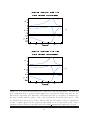
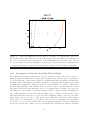
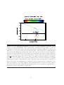
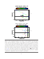
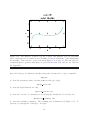
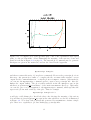
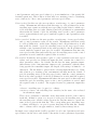
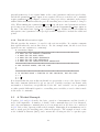
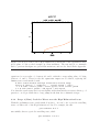
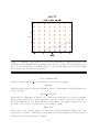
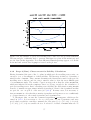
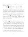
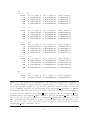
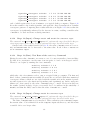
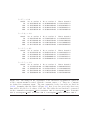
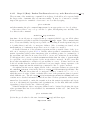
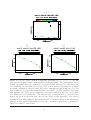
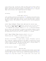
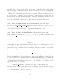
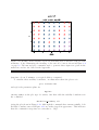
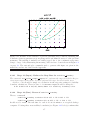
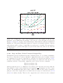
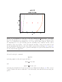
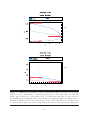
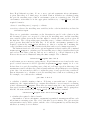
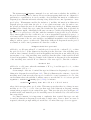
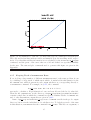
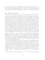
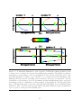
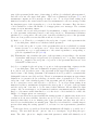
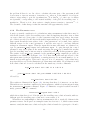
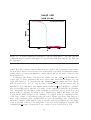
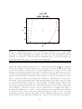
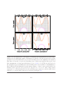
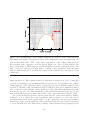
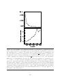
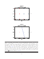
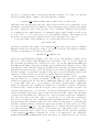
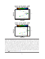
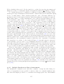
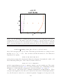
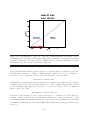
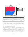
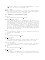
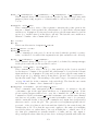
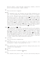
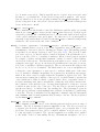
Figure 2.5: The Hopf bifurcation locus and two contours of constant wave period for
the problem demo, superimposed on a plot showing periodic travelling wave existence in
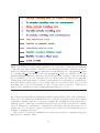
the control parameter–wave speed plane. A key illustrating the meaning of the various
colours and symbols is shown in Figure 2.4 on page 18. The run and plot commands used
to generate this figure are given in the main text, and are also listed in the Appendix.
2.1.2
Investigation of Periodic Travelling Wave Stability
The calculations and plots described above give a detailed account of the region of the A–c
parameter plane in which there are periodic travelling waves, but they give no information
about the stability of these waves, which is a fundamental issue in applications (Sherratt
& Smith, 2008). Wavetrain determines stability by calculating the eigenvalue spectrum
via numerical continuation, using the method of Rademacher et al (2007). Although a
detailed understanding of the method is not needed in order to use wavetrain, a brief
introduction will help users with their choice of computational constants. For a periodic
travelling wave, the system of equations satisfied by the (complex-valued) eigenfunctions
has coefficients that are periodic in the travelling wave coordinate. However, the eigenfunctions themselves need not be periodic; their amplitude must be periodic, but their
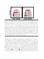
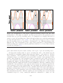
phase shift γ across one period of the wave is not constrained, and is the central player
in the method of Rademacher et al (2007). One begins by calculating the eigenvalues
for which γ = 0, i.e. those for which the corresponding eigenfunction is periodic with the
same period as the wave. This is done by discretising the eigenfunction equation and then
21