
1
AUTO-07P :
CONTINUATION AND BIFURCATION SOFTWARE
FOR ORDINARY DIFFERENTIAL EQUATIONS
Eusebius J. Doedel and Bart E. Oldeman
Concordia University
Montreal, Canada
with major contributions by
Alan R. Champneys (Bristol), Fabio Dercole (Milano), Thomas Fairgrieve (Toronto),
Yuri Kuznetsov (Utrecht), Randy Paffenroth (Pasadena),
Björn Sandstede (Brown), Xianjun Wang, and Chenghai Zhang.
January 2012
Contents
1 Installing AUTO.
1.1 Installation. . . . . . . . . . . . . . .
1.1.1 Installation on Linux/Unix . .
1.1.2 Installation on Mac OS X . .
1.1.3 Installation on Windows . . .
1.2 Restrictions on Problem Size. . . . .
1.3 Compatibility with Earlier Versions.
1.4 Parallel Version. . . . . . . . . . . .
2
3
4
Overview of Capabilities.
2.1 Summary. . . . . . . . . . . . . .
2.2 Algebraic Systems. . . . . . . . .
2.3 Ordinary Differential Equations.
2.4 Parabolic PDEs. . . . . . . . . .
2.5 Discretization. . . . . . . . . . .
User-Supplied Files.
3.1 The Equations-File xxx.f90, or
3.2 The Constants-File c.xxx . . .
3.3 User-Supplied Routines. . . . .
3.4 User-Supplied Derivatives. . . .
.
.
.
.
.
.
.
.
.
.
.
.
.
.
.
.
.
.
.
.
.
.
.
.
.
.
.
.
.
.
.
.
.
.
.
.
.
.
.
.
.
.
.
.
.
.
.
.
.
.
.
.
.
.
.
.
.
.
.
.
.
.
.
.
.
.
.
.
.
.
.
.
.
.
.
.
.
.
.
.
.
.
.
.
.
.
.
.
.
.
.
.
.
.
.
.
.
.
.
.
.
.
.
.
.
.
.
.
.
.
.
.
.
.
.
.
.
.
.
.
.
.
.
.
.
.
.
.
.
.
.
.
.
.
.
.
.
.
.
.
.
.
.
.
.
.
.
.
.
.
.
.
.
.
.
.
.
.
.
.
.
.
.
.
.
.
.
.
11
11
12
13
14
15
15
16
.
.
.
.
.
.
.
.
.
.
.
.
.
.
.
.
.
.
.
.
.
.
.
.
.
.
.
.
.
.
.
.
.
.
.
.
.
.
.
.
.
.
.
.
.
.
.
.
.
.
.
.
.
.
.
.
.
.
.
.
.
.
.
.
.
.
.
.
.
.
.
.
.
.
.
.
.
.
.
.
.
.
.
.
.
.
.
.
.
.
18
18
18
19
20
21
xxx.f, or xxx.c
. . . . . . . . . .
. . . . . . . . . .
. . . . . . . . . .
.
.
.
.
.
.
.
.
.
.
.
.
.
.
.
.
.
.
.
.
.
.
.
.
.
.
.
.
.
.
.
.
.
.
.
.
.
.
.
.
.
.
.
.
.
.
.
.
.
.
.
.
.
.
.
.
.
.
.
.
.
.
.
.
.
.
.
.
22
22
22
23
23
. . . . . . . . . . .
. . . . . . . . . . .
. . . . . . . . . . .
. . . . . . . . . . .
. . . . . . . . . . .
. . . . . . . . . . .
. . . . . . . . . . .
. . . . . . . . . . .
. . . . . . . . . . .
. . . . . . . . . . .
visualization tools.
. . . . . . . . . . .
.
.
.
.
.
.
.
.
.
.
.
.
.
.
.
.
.
.
.
.
.
.
.
.
.
.
.
.
.
.
.
.
.
.
.
.
.
.
.
.
.
.
.
.
.
.
.
.
25
25
25
26
30
30
34
37
41
45
46
46
46
.
.
.
.
.
.
.
.
.
.
.
.
.
.
.
.
.
.
.
.
.
.
.
.
.
.
.
.
.
.
.
.
.
.
.
.
.
.
.
.
Running AUTO using Python Commands.
4.1 Typographical Conventions . . . . . . . . . . . . . .
4.2 General Overview. . . . . . . . . . . . . . . . . . . .
4.3 First Example . . . . . . . . . . . . . . . . . . . . .
4.4 Scripting . . . . . . . . . . . . . . . . . . . . . . . .
4.5 Second Example . . . . . . . . . . . . . . . . . . . .
4.6 Extending the AUTO CLUI . . . . . . . . . . . . .
4.7 Bifurcation Diagram Objects . . . . . . . . . . . . .
4.7.1 Solutions . . . . . . . . . . . . . . . . . . . .
4.7.2 Summary and reference . . . . . . . . . . . . .
4.8 Importing data from Python or external tools. . . .
4.9 Exporting output data for use by Python or external
4.10 The .autorc or autorc File . . . . . . . . . . . . . . .
1
4.11
4.12
4.13
4.14
5
6
7
8
Plotting Tool . . . . . . . . . . . . . . . . . . . . . .
The Plotting Tool PLAUT04 . . . . . . . . . . . . .
Quick Reference . . . . . . . . . . . . . . . . . . . .
Reference . . . . . . . . . . . . . . . . . . . . . . .
4.14.1 Basic commands. . . . . . . . . . . . . . . . .
4.14.2 Plotting commands. . . . . . . . . . . . . . .
4.14.3 File-manipulation. . . . . . . . . . . . . . . .
4.14.4 Diagnostics. . . . . . . . . . . . . . . . . . . .
4.14.5 File-maintenance. . . . . . . . . . . . . . . . .
4.14.6 Copying a demo. . . . . . . . . . . . . . . . .
4.14.7 Python data structure manipulation functions.
4.14.8 Shell Commands. . . . . . . . . . . . . . . . .
Running AUTO using Unix Commands.
5.1 Basic commands. . . . . . . . . . . . . . .
5.2 Plotting commands. . . . . . . . . . . . .
5.3 File-manipulation. . . . . . . . . . . . . .
5.4 Diagnostics. . . . . . . . . . . . . . . . . .
5.5 File-editing. . . . . . . . . . . . . . . . . .
5.6 File-maintenance. . . . . . . . . . . . . .
5.7 HomCont commands. . . . . . . . . . . .
5.8 Copying a demo. . . . . . . . . . . . . . .
5.9 Viewing the manual. . . . . . . . . . . . .
.
.
.
.
.
.
.
.
.
.
.
.
.
.
.
.
.
.
.
.
.
.
.
.
.
.
.
.
.
.
.
.
.
.
.
.
.
.
.
.
.
.
.
.
.
.
.
.
.
.
.
.
.
.
.
.
.
.
.
.
.
.
.
.
.
.
.
.
.
.
.
.
.
.
.
.
.
.
.
.
.
.
.
.
.
.
.
.
.
.
.
.
.
.
.
.
.
.
.
.
.
.
.
.
.
.
.
.
.
.
.
.
.
.
.
.
.
.
.
.
.
.
.
.
.
.
.
.
.
.
.
.
.
.
.
.
.
.
.
.
.
.
.
.
.
.
.
.
.
.
.
.
.
.
.
.
.
.
.
.
.
.
.
.
.
.
.
.
.
.
.
.
.
.
.
.
.
.
.
.
.
.
.
.
.
.
.
.
.
.
.
.
.
.
.
.
.
.
.
.
.
.
.
.
.
.
.
.
.
.
.
.
.
.
.
.
.
.
.
.
.
.
.
.
.
.
.
.
.
.
.
.
.
.
.
.
.
.
.
.
.
.
.
.
.
.
.
.
.
.
.
.
.
.
.
.
.
.
.
.
.
.
.
.
.
.
.
.
.
.
.
.
.
.
.
.
.
.
.
.
.
.
.
.
.
.
.
.
.
.
.
.
.
.
.
.
.
.
.
.
.
.
.
.
.
.
.
.
.
.
.
.
.
.
.
.
.
.
.
.
.
.
.
.
.
.
.
.
.
.
.
.
.
.
.
.
.
.
.
.
.
.
.
.
.
.
.
.
.
.
.
.
.
.
.
.
.
.
.
.
47
50
50
53
53
56
56
57
59
63
63
65
.
.
.
.
.
.
.
.
.
66
66
67
67
68
70
70
72
72
72
Output Files.
73
The Graphics Programs PLAUT and PyPLAUT.
7.1 Basic PLAUT-Commands. . . . . . . . . . . . . .
7.2 Default Options. . . . . . . . . . . . . . . . . . . .
7.3 Other PLAUT-Commands. . . . . . . . . . . . . .
7.4 Printing PLAUT Files. . . . . . . . . . . . . . . .
.
.
.
.
.
.
.
.
.
.
.
.
.
.
.
.
.
.
.
.
.
.
.
.
.
.
.
.
.
.
.
.
.
.
.
.
.
.
.
.
.
.
.
.
.
.
.
.
.
.
.
.
.
.
.
.
.
.
.
.
.
.
.
.
76
76
77
78
78
The Graphics Program PLAUT04.
8.1 Quick start . . . . . . . . . . . . . . .
8.1.1 Starting and stopping Plaut04
8.1.2 Changing the “Type” . . . . . .
8.1.3 Changing the “Style” . . . . . .
8.1.4 Coordinate axes . . . . . . . . .
8.1.5 Options . . . . . . . . . . . . .
8.1.6 CR3BP animation . . . . . . .
8.1.7 Help . . . . . . . . . . . . . . .
8.1.8 Picking a point in the diagram .
8.1.9 Choosing the variables . . . . .
8.1.10 Choosing labels . . . . . . . . .
8.1.11 Coloring . . . . . . . . . . . . .
.
.
.
.
.
.
.
.
.
.
.
.
.
.
.
.
.
.
.
.
.
.
.
.
.
.
.
.
.
.
.
.
.
.
.
.
.
.
.
.
.
.
.
.
.
.
.
.
.
.
.
.
.
.
.
.
.
.
.
.
.
.
.
.
.
.
.
.
.
.
.
.
.
.
.
.
.
.
.
.
.
.
.
.
.
.
.
.
.
.
.
.
.
.
.
.
.
.
.
.
.
.
.
.
.
.
.
.
.
.
.
.
.
.
.
.
.
.
.
.
.
.
.
.
.
.
.
.
.
.
.
.
.
.
.
.
.
.
.
.
.
.
.
.
.
.
.
.
.
.
.
.
.
.
.
.
.
.
.
.
.
.
.
.
.
.
.
.
.
.
.
.
.
.
.
.
.
.
.
.
.
.
.
.
.
.
.
.
.
.
.
.
79
79
79
80
80
80
80
80
81
81
83
84
84
2
.
.
.
.
.
.
.
.
.
.
.
.
.
.
.
.
.
.
.
.
.
.
.
.
.
.
.
.
.
.
.
.
.
.
.
.
.
.
.
.
.
.
.
.
.
.
.
.
.
.
.
.
.
.
.
.
.
.
.
.
.
.
.
.
.
.
.
.
.
.
.
.
.
.
.
.
.
.
.
.
.
.
.
.
8.2
8.3
9
8.1.12 Number of periods to be animated
8.1.13 Changing the line/tube thickness .
8.1.14 Changing the animation speed . . .
8.1.15 Changing the background picture .
Setting up the resource file . . . . . . . . .
Example . . . . . . . . . . . . . . . . . . .
The Graphical User Interface GUI94.
9.1 General Overview. . . . . . . . . . . .
9.1.1 The Menu bar. . . . . . . . . .
9.1.2 The Define-Constants-buttons.
9.1.3 The Load-Constants-buttons. .
9.1.4 The Stop- and Exit-buttons. .
9.2 The Menu Bar. . . . . . . . . . . . . .
9.2.1 Equations-button. . . . . . . .
9.2.2 Edit-button. . . . . . . . . . .
9.2.3 Write-button. . . . . . . . . . .
9.2.4 Define-button. . . . . . . . . .
9.2.5 Run-button. . . . . . . . . . .
9.2.6 Save-button. . . . . . . . . . .
9.2.7 Append-button. . . . . . . . .
9.2.8 Plot-button. . . . . . . . . . .
9.2.9 Files-button. . . . . . . . . . .
9.2.10 Demos-button. . . . . . . . . .
9.2.11 Misc.-button. . . . . . . . . . .
9.2.12 Help-button. . . . . . . . . . .
9.3 Using the GUI. . . . . . . . . . . . . .
9.4 Customizing the GUI. . . . . . . . . .
9.4.1 Print-button. . . . . . . . . . .
9.4.2 GUI colors. . . . . . . . . . . .
9.4.3 On-line help. . . . . . . . . . .
10 Description of AUTO-Constants.
10.1 The AUTO-Constants File. . . .
10.2 Problem Constants. . . . . . . .
10.2.1 NDIM . . . . . . . . . . . .
10.2.2 NBC . . . . . . . . . . . . .
10.2.3 NINT . . . . . . . . . . . .
10.2.4 NPAR . . . . . . . . . . . .
10.2.5 JAC . . . . . . . . . . . . .
10.3 Discretization Constants. . . . .
10.3.1 NTST . . . . . . . . . . . .
10.3.2 NCOL . . . . . . . . . . . .
10.3.3 IAD . . . . . . . . . . . . .
10.4 Tolerances. . . . . . . . . . . . .
.
.
.
.
.
.
.
.
.
.
.
.
.
.
.
.
.
.
.
.
.
.
.
.
.
.
.
.
.
.
.
.
.
.
.
.
3
.
.
.
.
.
.
.
.
.
.
.
.
.
.
.
.
.
.
.
.
.
.
.
.
.
.
.
.
.
.
.
.
.
.
.
.
.
.
.
.
.
.
.
.
.
.
.
.
.
.
.
.
.
.
.
.
.
.
.
.
.
.
.
.
.
.
.
.
.
.
.
.
.
.
.
.
.
.
.
.
.
.
.
.
.
.
.
.
.
.
.
.
.
.
.
.
.
.
.
.
.
.
.
.
.
.
.
.
.
.
.
.
.
.
.
.
.
.
.
.
.
.
.
.
.
.
.
.
.
.
.
.
.
.
.
.
.
.
.
.
.
.
.
.
.
.
.
.
.
.
.
.
.
.
.
.
.
.
.
.
.
.
.
.
.
.
.
.
.
.
.
.
.
.
.
.
.
.
.
.
.
.
.
.
.
.
.
.
.
.
.
.
.
.
.
.
.
.
.
.
.
.
.
.
.
.
.
.
.
.
.
.
.
.
.
.
.
.
.
.
.
.
.
.
.
.
.
.
.
.
.
.
.
.
.
.
.
.
.
.
.
.
.
.
.
.
.
.
.
.
.
.
.
.
.
.
.
.
.
.
.
.
.
.
.
.
.
.
.
.
.
.
.
.
.
.
.
.
.
.
.
.
.
.
.
.
.
.
.
.
.
.
.
.
.
.
.
.
.
.
.
.
.
.
.
.
.
.
.
.
.
.
.
.
.
.
.
.
.
.
.
.
.
.
.
.
.
.
.
.
.
.
.
.
.
.
.
.
.
.
.
.
.
.
.
.
.
.
.
.
.
.
.
.
.
.
.
.
.
.
.
.
.
.
.
.
.
.
.
.
.
.
.
.
.
.
.
.
.
.
.
.
.
.
.
.
.
.
.
.
.
.
.
.
.
.
.
.
.
.
.
.
.
.
.
.
.
.
.
.
.
.
.
.
.
.
.
.
.
.
.
.
.
.
.
.
.
.
.
.
.
.
.
.
.
.
.
.
.
.
.
.
.
.
.
.
.
.
.
.
.
.
.
.
.
.
.
.
.
.
.
.
.
.
.
.
.
.
.
.
.
.
.
.
.
.
.
.
.
.
.
.
.
.
.
.
.
.
.
.
.
.
.
.
.
.
.
.
.
.
.
.
.
.
.
.
.
.
.
.
.
.
.
.
.
.
.
.
.
.
.
.
.
.
.
.
.
.
.
.
.
.
.
.
.
.
.
.
.
.
.
.
.
.
.
.
.
.
.
.
.
.
.
.
.
.
.
.
.
.
.
.
.
.
.
.
.
.
.
.
.
.
.
.
.
.
.
.
.
.
.
.
.
.
.
.
.
.
.
.
.
.
.
.
.
.
.
.
.
.
.
.
.
.
.
.
.
.
.
.
.
.
.
.
.
.
.
.
.
.
.
.
.
.
.
.
.
.
.
.
.
.
.
.
.
.
.
.
.
.
.
.
.
.
.
.
.
.
.
.
.
.
.
.
.
.
.
.
.
.
.
.
.
.
.
.
.
.
.
.
.
.
.
.
.
.
.
.
.
.
.
.
.
.
.
.
.
.
.
.
.
.
.
.
.
.
.
.
.
.
.
.
.
.
.
.
.
.
.
.
.
.
.
.
.
.
.
.
.
.
.
.
.
.
.
.
.
.
.
.
.
.
.
.
.
.
.
.
.
.
.
.
.
.
.
.
.
.
.
.
.
.
.
.
.
.
.
.
.
.
.
.
.
.
.
.
.
.
.
.
.
.
.
.
.
.
.
.
.
.
.
.
.
.
.
.
.
.
.
.
.
.
.
.
.
.
.
.
.
.
.
.
.
.
.
.
.
.
.
.
.
.
.
.
.
.
.
.
.
.
.
.
.
.
.
.
.
.
.
.
.
.
.
.
.
.
.
.
.
.
.
.
.
.
.
.
.
.
.
.
.
.
.
.
.
.
.
.
.
.
.
.
.
.
.
.
.
.
.
.
.
.
.
.
.
.
.
.
.
.
.
.
.
.
.
.
.
.
.
.
.
.
.
.
.
.
84
85
85
85
85
89
.
.
.
.
.
.
.
.
.
.
.
.
.
.
.
.
.
.
.
.
.
.
.
92
92
92
92
93
93
93
93
93
93
93
94
94
94
94
94
94
95
95
95
95
95
95
96
.
.
.
.
.
.
.
.
.
.
.
.
97
97
98
98
98
98
98
98
98
98
99
99
99
10.5
10.6
10.7
10.8
10.9
10.4.1 EPSL . . . . . . . . . . . . . . . .
10.4.2 EPSU . . . . . . . . . . . . . . . .
10.4.3 EPSS . . . . . . . . . . . . . . . .
10.4.4 ITMX . . . . . . . . . . . . . . . .
10.4.5 NWTN . . . . . . . . . . . . . . . .
10.4.6 ITNW . . . . . . . . . . . . . . . .
Continuation Step Size. . . . . . . . . .
10.5.1 DS . . . . . . . . . . . . . . . . .
10.5.2 DSMIN . . . . . . . . . . . . . . .
10.5.3 DSMAX . . . . . . . . . . . . . . .
10.5.4 IADS . . . . . . . . . . . . . . . .
10.5.5 THL . . . . . . . . . . . . . . . . .
10.5.6 THU . . . . . . . . . . . . . . . . .
Diagram Limits. . . . . . . . . . . . . .
10.6.1 STOP . . . . . . . . . . . . . . . .
10.6.2 NMX . . . . . . . . . . . . . . . . .
10.6.3 RL0 . . . . . . . . . . . . . . . . .
10.6.4 RL1 . . . . . . . . . . . . . . . . .
10.6.5 A0 . . . . . . . . . . . . . . . . .
10.6.6 A1 . . . . . . . . . . . . . . . . .
Free Parameters. . . . . . . . . . . . . .
10.7.1 ICP . . . . . . . . . . . . . . . . .
10.7.2 Fixed points. . . . . . . . . . . .
10.7.3 Periodic solutions and rotations.
10.7.4 Folds and Hopf bifurcations. . .
10.7.5 Folds and period-doublings. . . .
10.7.6 Boundary value problems. . . . .
10.7.7 Boundary value folds. . . . . . .
10.7.8 Optimization problems. . . . . .
10.7.9 Internal free parameters. . . . .
10.7.10 Parameter overspecification. . . .
Computation Constants. . . . . . . . . .
10.8.1 ILP . . . . . . . . . . . . . . . . .
10.8.2 SP . . . . . . . . . . . . . . . . .
10.8.3 ISP . . . . . . . . . . . . . . . . .
10.8.4 ISW . . . . . . . . . . . . . . . . .
10.8.5 MXBF . . . . . . . . . . . . . . . .
10.8.6 s . . . . . . . . . . . . . . . . . .
10.8.7 dat . . . . . . . . . . . . . . . . .
10.8.8 U . . . . . . . . . . . . . . . . . .
10.8.9 PAR . . . . . . . . . . . . . . . . .
10.8.10 IRS . . . . . . . . . . . . . . . . .
10.8.11 TY . . . . . . . . . . . . . . . . .
10.8.12 IPS . . . . . . . . . . . . . . . . .
Output Control. . . . . . . . . . . . . .
4
.
.
.
.
.
.
.
.
.
.
.
.
.
.
.
.
.
.
.
.
.
.
.
.
.
.
.
.
.
.
.
.
.
.
.
.
.
.
.
.
.
.
.
.
.
.
.
.
.
.
.
.
.
.
.
.
.
.
.
.
.
.
.
.
.
.
.
.
.
.
.
.
.
.
.
.
.
.
.
.
.
.
.
.
.
.
.
.
.
.
.
.
.
.
.
.
.
.
.
.
.
.
.
.
.
.
.
.
.
.
.
.
.
.
.
.
.
.
.
.
.
.
.
.
.
.
.
.
.
.
.
.
.
.
.
.
.
.
.
.
.
.
.
.
.
.
.
.
.
.
.
.
.
.
.
.
.
.
.
.
.
.
.
.
.
.
.
.
.
.
.
.
.
.
.
.
.
.
.
.
.
.
.
.
.
.
.
.
.
.
.
.
.
.
.
.
.
.
.
.
.
.
.
.
.
.
.
.
.
.
.
.
.
.
.
.
.
.
.
.
.
.
.
.
.
.
.
.
.
.
.
.
.
.
.
.
.
.
.
.
.
.
.
.
.
.
.
.
.
.
.
.
.
.
.
.
.
.
.
.
.
.
.
.
.
.
.
.
.
.
.
.
.
.
.
.
.
.
.
.
.
.
.
.
.
.
.
.
.
.
.
.
.
.
.
.
.
.
.
.
.
.
.
.
.
.
.
.
.
.
.
.
.
.
.
.
.
.
.
.
.
.
.
.
.
.
.
.
.
.
.
.
.
.
.
.
.
.
.
.
.
.
.
.
.
.
.
.
.
.
.
.
.
.
.
.
.
.
.
.
.
.
.
.
.
.
.
.
.
.
.
.
.
.
.
.
.
.
.
.
.
.
.
.
.
.
.
.
.
.
.
.
.
.
.
.
.
.
.
.
.
.
.
.
.
.
.
.
.
.
.
.
.
.
.
.
.
.
.
.
.
.
.
.
.
.
.
.
.
.
.
.
.
.
.
.
.
.
.
.
.
.
.
.
.
.
.
.
.
.
.
.
.
.
.
.
.
.
.
.
.
.
.
.
.
.
.
.
.
.
.
.
.
.
.
.
.
.
.
.
.
.
.
.
.
.
.
.
.
.
.
.
.
.
.
.
.
.
.
.
.
.
.
.
.
.
.
.
.
.
.
.
.
.
.
.
.
.
.
.
.
.
.
.
.
.
.
.
.
.
.
.
.
.
.
.
.
.
.
.
.
.
.
.
.
.
.
.
.
.
.
.
.
.
.
.
.
.
.
.
.
.
.
.
.
.
.
.
.
.
.
.
.
.
.
.
.
.
.
.
.
.
.
.
.
.
.
.
.
.
.
.
.
.
.
.
.
.
.
.
.
.
.
.
.
.
.
.
.
.
.
.
.
.
.
.
.
.
.
.
.
.
.
.
.
.
.
.
.
.
.
.
.
.
.
.
.
.
.
.
.
.
.
.
.
.
.
.
.
.
.
.
.
.
.
.
.
.
.
.
.
.
.
.
.
.
.
.
.
.
.
.
.
.
.
.
.
.
.
.
.
.
.
.
.
.
.
.
.
.
.
.
.
.
.
.
.
.
.
.
.
.
.
.
.
.
.
.
.
.
.
.
.
.
.
.
.
.
.
.
.
.
.
.
.
.
.
.
.
.
.
.
.
.
.
.
.
.
.
.
.
.
.
.
.
.
.
.
.
.
.
.
.
.
.
.
.
.
.
.
.
.
.
.
.
.
.
.
.
.
.
.
.
.
.
.
.
.
.
.
.
.
.
.
.
.
.
.
.
.
.
.
.
.
.
.
.
.
.
.
.
.
.
.
.
.
.
.
.
.
.
.
.
.
.
.
.
.
.
.
.
.
.
.
.
.
.
.
.
.
.
.
.
.
.
.
.
.
.
.
.
.
.
.
.
.
.
.
.
.
.
.
.
.
.
.
.
.
.
.
.
.
.
.
.
.
.
.
.
.
.
.
.
.
.
.
.
.
.
.
.
.
.
.
.
.
.
.
.
.
.
.
.
.
.
.
.
.
.
.
.
.
.
.
.
.
.
.
.
.
.
.
.
.
.
.
.
.
.
.
.
.
.
.
.
.
.
.
.
.
.
.
.
.
.
.
.
.
.
.
.
.
.
.
.
.
.
.
.
.
.
.
.
.
.
.
.
.
.
.
.
.
.
.
.
.
.
.
.
.
.
.
.
.
.
.
.
.
.
.
.
.
.
.
.
.
.
.
.
.
99
99
99
99
100
100
100
100
100
100
101
101
101
101
102
102
102
102
102
102
103
103
103
103
103
104
104
104
104
105
105
105
105
106
106
106
107
107
107
107
108
108
108
108
110
10.9.1 unames . .
10.9.2 parnames
10.9.3 e . . . . .
10.9.4 sv . . . .
10.9.5 NPR . . . .
10.9.6 IBR . . . .
10.9.7 LAB . . . .
10.9.8 IIS . . . .
10.9.9 IID . . . .
10.9.10 IPLT . . .
10.9.11 UZR . . . .
10.9.12 UZSTOP . .
10.10 Quick reference .
.
.
.
.
.
.
.
.
.
.
.
.
.
.
.
.
.
.
.
.
.
.
.
.
.
.
.
.
.
.
.
.
.
.
.
.
.
.
.
.
.
.
.
.
.
.
.
.
.
.
.
.
.
.
.
.
.
.
.
.
.
.
.
.
.
.
.
.
.
.
.
.
.
.
.
.
.
.
.
.
.
.
.
.
.
.
.
.
.
.
.
.
.
.
.
.
.
.
.
.
.
.
.
.
.
.
.
.
.
.
.
.
.
.
.
.
.
.
.
.
.
.
.
.
.
.
.
.
.
.
.
.
.
.
.
.
.
.
.
.
.
.
.
.
.
.
.
.
.
.
.
.
.
.
.
.
.
.
.
.
.
.
.
.
.
.
.
.
.
.
.
.
.
.
.
.
.
.
.
.
.
.
.
.
.
.
.
.
.
.
.
.
.
.
.
.
.
.
.
.
.
.
.
.
.
.
.
.
.
.
.
.
.
.
.
.
.
.
.
.
.
.
.
.
.
.
.
.
.
.
.
.
.
.
.
.
.
.
.
.
.
.
.
.
.
.
.
.
.
.
.
.
.
.
.
.
.
.
.
.
.
.
.
.
.
.
.
.
.
.
.
.
.
.
.
.
.
.
.
.
.
.
.
.
.
.
.
.
.
.
.
.
.
.
.
.
.
.
.
.
.
.
.
.
.
.
.
.
.
.
.
.
.
.
.
.
.
.
.
.
.
.
.
.
.
.
.
.
.
.
.
.
.
.
.
.
.
.
.
.
.
.
.
.
.
.
.
.
.
.
.
.
.
.
.
.
.
.
.
.
.
.
.
.
.
.
.
.
.
.
.
.
.
.
.
.
.
.
.
.
.
.
.
.
.
.
.
.
.
.
.
.
.
.
.
.
.
.
.
.
.
.
.
.
.
.
.
.
.
.
.
.
.
.
.
.
.
.
.
.
.
.
.
.
.
.
.
.
.
.
.
.
.
.
.
.
.
.
.
.
.
.
.
.
.
.
.
.
.
.
.
.
.
.
.
110
110
110
110
111
111
111
111
111
112
113
113
115
11 Notes on Using AUTO.
11.1 Restrictions on the Use of PAR.
11.2 Efficiency. . . . . . . . . . . . .
11.3 Correctness of Results. . . . . .
11.4 Bifurcation Points and Folds. .
11.5 Floquet Multipliers. . . . . . .
11.6 Memory Requirements. . . . .
.
.
.
.
.
.
.
.
.
.
.
.
.
.
.
.
.
.
.
.
.
.
.
.
.
.
.
.
.
.
.
.
.
.
.
.
.
.
.
.
.
.
.
.
.
.
.
.
.
.
.
.
.
.
.
.
.
.
.
.
.
.
.
.
.
.
.
.
.
.
.
.
.
.
.
.
.
.
.
.
.
.
.
.
.
.
.
.
.
.
.
.
.
.
.
.
.
.
.
.
.
.
.
.
.
.
.
.
.
.
.
.
.
.
.
.
.
.
.
.
.
.
.
.
.
.
.
.
.
.
.
.
.
.
.
.
.
.
.
.
.
.
.
.
.
.
.
.
.
.
.
.
.
.
.
.
.
.
.
.
.
.
116
116
117
117
117
118
118
12 AUTO Demos : Tutorial.
12.1 Introduction. . . . . . . . . . . . . . . . . .
12.2 cusp : A Tutorial Demo. . . . . . . . . . . .
12.3 Copying the Demo Files. . . . . . . . . . .
12.4 Executing all Runs Automatically. . . . . .
12.5 Plotting the Results with AUTO. . . . . . .
12.6 Plotting the Results with AUTO in 3D. . .
12.7 Exporting the Results for different plotters.
12.8 ab : A Programmed Demo. . . . . . . . . .
.
.
.
.
.
.
.
.
.
.
.
.
.
.
.
.
.
.
.
.
.
.
.
.
.
.
.
.
.
.
.
.
.
.
.
.
.
.
.
.
.
.
.
.
.
.
.
.
.
.
.
.
.
.
.
.
.
.
.
.
.
.
.
.
.
.
.
.
.
.
.
.
.
.
.
.
.
.
.
.
.
.
.
.
.
.
.
.
.
.
.
.
.
.
.
.
.
.
.
.
.
.
.
.
.
.
.
.
.
.
.
.
.
.
.
.
.
.
.
.
.
.
.
.
.
.
.
.
.
.
.
.
.
.
.
.
.
.
.
.
.
.
.
.
.
.
.
.
.
.
.
.
.
.
.
.
.
.
.
.
119
120
120
120
121
123
124
124
126
.
.
.
.
127
127
128
129
130
.
.
.
.
.
.
131
132
133
137
140
141
142
13 AUTO Demos : Fixed points.
13.1 enz : Stationary Solutions of an Enzyme Model. . .
13.2 dd2 : Fixed Points of a Discrete Dynamical System.
13.3 log : The Logistic Map. . . . . . . . . . . . . . . . .
13.4 hen: The Hénon Map. . . . . . . . . . . . . . . . . .
14 AUTO Demos : Periodic solutions.
14.1 lrz : The Lorenz Equations. . . . . . . . . . .
14.2 abc : The A → B → C Reaction. . . . . . . .
14.3 pp2 : A 2D Predator-Prey Model. . . . . . .
14.4 lor : Starting an Orbit from Numerical Data.
14.5 frc : A Periodically Forced System. . . . . . .
14.6 ppp : Continuation of Hopf Bifurcations. . . .
5
.
.
.
.
.
.
.
.
.
.
.
.
.
.
.
.
.
.
.
.
.
.
.
.
.
.
.
.
.
.
.
.
.
.
.
.
.
.
.
.
.
.
.
.
.
.
.
.
.
.
.
.
.
.
.
.
.
.
.
.
.
.
.
.
.
.
.
.
.
.
.
.
.
.
.
.
.
.
.
.
.
.
.
.
.
.
.
.
.
.
.
.
.
.
.
.
.
.
.
.
.
.
.
.
.
.
.
.
.
.
.
.
.
.
.
.
.
.
.
.
.
.
.
.
.
.
.
.
.
.
.
.
.
.
.
.
.
.
.
.
.
.
.
.
.
.
.
.
.
.
.
.
.
.
.
.
.
.
.
.
.
.
.
.
14.7
14.8
14.9
14.10
14.11
14.12
14.13
14.14
14.15
plp : Fold Continuation for Periodic Solutions. . . . . . . . . . . . . . .
ph1 : Phase-Shifting using Continuation. . . . . . . . . . . . . . . . . . .
pp3 : Periodic Families and Loci of Hopf Points. . . . . . . . . . . . . .
tor : Detection of Torus Bifurcations. . . . . . . . . . . . . . . . . . . .
pen : Rotations of Coupled Pendula. . . . . . . . . . . . . . . . . . . . .
chu : A Non-Smooth System (Chua’s Circuit). . . . . . . . . . . . . . .
phs : Effect of the Phase Condition. . . . . . . . . . . . . . . . . . . . .
ivp : Time Integration with Euler’s Method. . . . . . . . . . . . . . . . .
r3b : The Circular Restricted 3-Body Problem (CR3BP). . . . . . . . .
14.15.1 Computation of Periodic Solutions of the CR3BP . . . . . . . . .
14.15.2 Computing Unstable Manifolds of Periodic Orbits in the CR3BP .
15 AUTO Demos : BVP.
15.1 exp : Bratu’s Equation. . . . . . . . . . . . . . . . . . . . . .
15.2 int : Boundary and Integral Constraints. . . . . . . . . . . . .
15.3 bvp : A Nonlinear ODE Eigenvalue Problem. . . . . . . . . .
15.4 lin : A Linear ODE Eigenvalue Problem. . . . . . . . . . . . .
15.5 non : A Non-Autonomous BVP. . . . . . . . . . . . . . . . .
15.6 kar : The Von Karman Swirling Flows. . . . . . . . . . . . . .
15.7 spb : A Singularly-Perturbed BVP. . . . . . . . . . . . . . . .
15.8 ezp : Complex Bifurcation in a BVP. . . . . . . . . . . . . . .
15.9 um2 : Basic computation of a 2D unstable manifold. . . . . .
15.10 um3 : A 2D unstable manifold in 3D. . . . . . . . . . . . . .
15.11 p2c : Point to cycle connections. . . . . . . . . . . . . . . . .
15.12 c2c : Cycle to cycle connections. . . . . . . . . . . . . . . . .
15.13 pcl : Lorenz: Point-to-cycle connections with Lin’s method. .
15.14 snh : SNH with Global reinjection: Point-to-cycle connections
15.14.1 The homoclinic point-to-point connection. . . . . . . .
15.14.2 The codimension-one point-to-cycle connection. . . . .
15.14.3 The codimension-zero point-to-cycle connection. . . . .
15.15 fnc : Canards in the FitzHugh-Nagumo system. . . . . . . . .
16 AUTO Demos : Parabolic PDEs.
16.1 pd1 : Stationary States (1D Problem). . . . . .
16.2 pd2 : Stationary States (2D Problem). . . . . .
16.3 wav : Periodic Waves. . . . . . . . . . . . . . .
16.4 brc : Chebyshev Collocation in Space. . . . . .
16.5 brf : Finite Differences in Space. . . . . . . . .
16.6 bru : Euler Time Integration (the Brusselator).
.
.
.
.
.
.
.
.
.
.
.
.
.
.
.
.
.
.
.
.
.
.
.
.
.
.
.
.
.
.
.
.
.
.
.
.
.
.
.
.
.
.
.
.
.
.
.
.
. . . . . .
. . . . . .
. . . . . .
. . . . . .
. . . . . .
. . . . . .
. . . . . .
. . . . . .
. . . . . .
. . . . . .
. . . . . .
. . . . . .
. . . . . .
with Lin’s
. . . . . .
. . . . . .
. . . . . .
. . . . . .
.
.
.
.
.
.
.
.
.
.
.
.
.
.
.
.
.
.
.
.
.
.
.
.
.
.
.
.
.
.
.
.
.
.
.
.
.
.
.
.
.
.
.
.
.
.
.
.
.
.
.
.
.
.
.
.
.
.
.
.
.
.
.
.
.
.
.
.
.
.
.
.
.
.
.
.
.
.
.
.
143
144
145
147
148
150
151
152
153
153
154
161
. . . . 161
. . . . 162
. . . . 163
. . . . 164
. . . . 165
. . . . 166
. . . . 167
. . . . 168
. . . . 169
. . . . 170
. . . . 171
. . . . 171
. . . . 172
method.174
. . . . 174
. . . . 175
. . . . 176
. . . . 178
.
.
.
.
.
.
.
.
.
.
.
.
.
.
.
.
.
.
.
.
.
.
.
.
181
182
183
184
185
186
187
17 AUTO Demos : Optimization.
188
17.1 opt : A Model Algebraic Optimization Problem. . . . . . . . . . . . . . . . . . 189
17.2 ops : Optimization of Periodic Solutions. . . . . . . . . . . . . . . . . . . . . . . 190
17.3 obv : Optimization for a BVP. . . . . . . . . . . . . . . . . . . . . . . . . . . . 194
6
18 AUTO Demos : Connecting orbits.
196
18.1 fsh : A Saddle-Node Connection. . . . . . . . . . . . . . . . . . . . . . . . . . . 197
18.2 nag : A Saddle-Saddle Connection. . . . . . . . . . . . . . . . . . . . . . . . . . 198
18.3 stw : Continuation of Sharp Traveling Waves. . . . . . . . . . . . . . . . . . . . 199
19 AUTO Demos : Miscellaneous.
19.1 pvl : Use of the Routine PVLS. . . . . . . . . . . . . . . . . . . . . . . . . . .
19.2 ext : Spurious Solutions to BVP. . . . . . . . . . . . . . . . . . . . . . . . . . .
19.3 tim : A Test Problem for Timing AUTO. . . . . . . . . . . . . . . . . . . . . .
201
202
203
204
20 HomCont.
20.1 Introduction. . . . . . . . . . . . . .
20.2 HomCont Files and Routines. . . . .
20.3 HomCont-Constants. . . . . . . . . .
20.3.1 NUNSTAB . . . . . . . . . . . .
20.3.2 NSTAB . . . . . . . . . . . . .
20.3.3 IEQUIB . . . . . . . . . . . . .
20.3.4 ITWIST . . . . . . . . . . . . .
20.3.5 ISTART . . . . . . . . . . . . .
20.3.6 IREV . . . . . . . . . . . . . .
20.3.7 IFIXED . . . . . . . . . . . . .
20.3.8 IPSI . . . . . . . . . . . . . .
20.4 Restrictions on HomCont Constants.
20.5 Restrictions on the Use of PAR. . . .
20.6 Test Functions. . . . . . . . . . . . .
20.7 Starting Strategies. . . . . . . . . . .
20.8 Notes on Running HomCont Demos.
.
.
.
.
.
.
.
.
.
.
.
.
.
.
.
.
.
.
.
.
.
.
.
.
.
.
.
.
.
.
.
.
.
.
.
.
.
.
.
.
.
.
.
.
.
.
.
.
.
.
.
.
.
.
.
.
.
.
.
.
.
.
.
.
.
.
.
.
.
.
.
.
.
.
.
.
.
.
.
.
.
.
.
.
.
.
.
.
.
.
.
.
.
.
.
.
.
.
.
.
.
.
.
.
.
.
.
.
.
.
.
.
.
.
.
.
.
.
.
.
.
.
.
.
.
.
.
.
.
.
.
.
.
.
.
.
.
.
.
.
.
.
.
.
.
.
.
.
.
.
.
.
.
.
.
.
.
.
.
.
.
.
.
.
.
.
.
.
.
.
.
.
.
.
.
.
.
.
.
.
.
.
.
.
.
.
.
.
.
.
.
.
.
.
.
.
.
.
.
.
.
.
.
.
.
.
.
.
.
.
.
.
.
.
.
.
.
.
.
.
.
.
.
.
.
.
.
.
.
.
.
.
.
.
.
.
.
.
.
.
.
.
.
.
.
.
.
.
.
.
.
.
.
.
.
.
.
.
.
.
.
.
.
.
.
.
.
.
.
.
.
.
.
.
.
.
.
.
.
.
.
.
.
.
.
.
.
.
.
.
.
.
.
.
.
.
.
.
.
.
.
.
.
.
.
.
.
.
.
.
.
.
.
.
.
.
.
.
.
.
.
.
.
.
.
.
.
.
.
.
.
.
.
.
.
.
.
.
.
.
.
.
.
.
.
.
.
.
.
.
.
.
.
.
.
.
.
.
.
.
.
.
.
.
.
.
.
.
.
.
.
.
.
.
.
.
.
.
.
.
.
.
.
.
205
205
205
206
206
206
206
207
207
208
208
208
208
209
209
211
212
21 HomCont Demo : san.
21.1 Sandstede’s Model. . . . . . . . . . .
21.2 Inclination Flip. . . . . . . . . . . . .
21.3 Non-orientable Resonant Eigenvalues.
21.4 Orbit Flip. . . . . . . . . . . . . . . .
21.5 Detailed AUTO-Commands. . . . .
.
.
.
.
.
.
.
.
.
.
.
.
.
.
.
.
.
.
.
.
.
.
.
.
.
.
.
.
.
.
.
.
.
.
.
.
.
.
.
.
.
.
.
.
.
.
.
.
.
.
.
.
.
.
.
.
.
.
.
.
.
.
.
.
.
.
.
.
.
.
.
.
.
.
.
.
.
.
.
.
.
.
.
.
.
.
.
.
.
.
.
.
.
.
.
.
.
.
.
.
.
.
.
.
.
.
.
.
.
.
.
.
.
.
.
.
.
.
.
.
214
214
214
216
216
217
.
.
.
.
.
220
220
220
222
223
223
22 HomCont Demo : mtn.
22.1 A Predator-Prey Model with Immigration. . . . . . . .
22.2 Continuation of Central Saddle-Node Homoclinics. . . .
22.3 Switching between Saddle-Node and Saddle Homoclinic
22.4 Three-Parameter Continuation. . . . . . . . . . . . . .
22.5 Detailed AUTO-Commands. . . . . . . . . . . . . . .
. . . . .
. . . . .
Orbits. .
. . . . .
. . . . .
.
.
.
.
.
.
.
.
.
.
.
.
.
.
.
.
.
.
.
.
.
.
.
.
.
.
.
.
.
.
.
.
.
.
.
.
.
.
.
.
23 HomCont Demo : kpr.
226
23.1 Koper’s Extended Van der Pol Model. . . . . . . . . . . . . . . . . . . . . . . . 226
23.2 The Primary Branch of Homoclinics. . . . . . . . . . . . . . . . . . . . . . . . . 226
7
23.3 More Accuracy and Saddle-Node Homoclinic Orbits. . . . . . . . . . . . . . . . 230
23.4 Three-Parameter Continuation. . . . . . . . . . . . . . . . . . . . . . . . . . . . 233
23.5 Detailed AUTO-Commands. . . . . . . . . . . . . . . . . . . . . . . . . . . . . 234
24 HomCont Demo : cir.
236
24.1 Electronic Circuit of Freire et al. . . . . . . . . . . . . . . . . . . . . . . . . . . 236
24.2 Detailed AUTO-Commands. . . . . . . . . . . . . . . . . . . . . . . . . . . . . 239
25 HomCont Demo : she.
240
25.1 A Heteroclinic Example. . . . . . . . . . . . . . . . . . . . . . . . . . . . . . . . 240
25.2 Detailed AUTO-Commands. . . . . . . . . . . . . . . . . . . . . . . . . . . . . 241
26 HomCont Demo : rev.
26.1 A Reversible System. . . . . . . . . .
26.2 An R1 -Reversible Homoclinic Solution.
26.3 An R2 -Reversible Homoclinic Solution.
26.4 Detailed AUTO-Commands. . . . . .
.
.
.
.
.
.
.
.
.
.
.
.
.
.
.
.
.
.
.
.
.
.
.
.
.
.
.
.
.
.
.
.
.
.
.
.
.
.
.
.
.
.
.
.
.
.
.
.
.
.
.
.
.
.
.
.
.
.
.
.
.
.
.
.
.
.
.
.
.
.
.
.
.
.
.
.
.
.
.
.
.
.
.
.
.
.
.
.
.
.
.
.
243
243
243
244
246
27 HomCont Demo : Homoclinic branch switching.
248
27.1 Branch switching at an inclination flip in Sandstede’s model. . . . . . . . . . . 248
27.2 Branch switching for a Shil’nikov type homoclinic orbit in the FitzHugh-Nagumo
equations. . . . . . . . . . . . . . . . . . . . . . . . . . . . . . . . . . . . . . . . 255
27.3 Branch switching to a 3-homoclinic orbit in a 5th-order Korteweg-De Vries model258
8
Preface
This is a guide to the software package AUTO for continuation and bifurcation problems in ordinary differential equations. Earlier versions of AUTO were described in Doedel (1981), Doedel
& Kernévez (1986a), Doedel & Wang (1995), Wang & Doedel (1995), Doedel, Champneys,
Fairgrieve, Kuznetsov, Sandstede & Wang (1997), Doedel, Paffenroth, Champneys, Fairgrieve,
Kuznetsov, Oldeman, Sandstede & Wang (2000). For a description of the basic algorithms see
Doedel, Keller & Kernévez (1991a), Doedel, Keller & Kernévez (1991b). AUTO incorporates the
HomCont algorithms of Champneys & Kuznetsov (1994), Champneys, Kuznetsov & Sandstede
(1996) for the bifurcation analysis of homoclinic orbits, and the BPcont algorithms of Dercole
(2008) for the continuation of branch points in both symmetric and non-symmetric problems.
The Floquet multiplier algorithms were written by Fairgrieve (1994), Fairgrieve & Jepson (1991).
A GUI was written by Wang (1994). The Python CLUI is the work of Randy Paffenroth.
Acknowledgments
The first author is much indebted to H. B. Keller of the California Institute of Technology for
his inspiration, encouragement and support. He is also thankful to AUTO users and research
collaborators who have directly or indirectly contributed to its development, in particular, Jean
Pierre Kernévez, UTC, Compiègne, France; Don Aronson, University of Minnesota, Minneapolis;
Hans Othmer, University of Utah; and Frank Schilder, University of Surrey. Some material
in this document related to the computation of connecting orbits was developed with Mark
Friedman, University of Alabama, Huntsville. Also acknowledged is the work of Nguyen Thanh
Long, Concordia University, Montreal, on the graphics program PLAUT. Special thanks are due
to Sheila Shull, California Institute of Technology, for her cheerful assistance in the distribution
of AUTO over a long period of time. Over the years, the development of AUTO has been
supported by various agencies through the California Institute of Technology, and by research
grants from NSERC (Canada).
The development of HomCont has benefitted from help and advice from, among others, W.J. Beyn, Universität Bielefeld, M. J. Friedman, University of Alabama, A. Rucklidge, University
of Cambridge, M. Koper, University of Utrecht, C. J. Budd, University of Bath, and Financial
support for this collaboration was also received from the U.K. Engineering and Physical Science
Research Council and the Nuffield Foundation.
9
License
AUTO is available under the terms of the BSD license:
c 1979–2007, E. J. Doedel, California Institute of Technology, and Concordia University. All rights
Copyright reserved.
Redistribution and use in source and binary forms, with or without modification, are permitted provided that
the following conditions are met:
• Redistributions of source code must retain the above copyright notice, this list of conditions and the
following disclaimer.
• Redistributions in binary form must reproduce the above copyright notice, this list of conditions and the
following disclaimer listed in this license in the documentation and/or other materials provided with the
distribution.
• Neither the name of the copyright holders nor the names of its contributors may be used to endorse or
promote products derived from this software without specific prior written permission.
THIS SOFTWARE IS PROVIDED BY THE COPYRIGHT HOLDERS AND CONTRIBUTORS ”AS IS” AND
ANY EXPRESS OR IMPLIED WARRANTIES, INCLUDING, BUT NOT LIMITED TO, THE IMPLIED WARRANTIES OF MERCHANTABILITY AND FITNESS FOR A PARTICULAR PURPOSE ARE DISCLAIMED.
IN NO EVENT SHALL THE COPYRIGHT OWNER OR CONTRIBUTORS BE LIABLE FOR ANY DIRECT,
INDIRECT, INCIDENTAL, SPECIAL, EXEMPLARY, OR CONSEQUENTIAL DAMAGES (INCLUDING,
BUT NOT LIMITED TO, PROCUREMENT OF SUBSTITUTE GOODS OR SERVICES; LOSS OF USE,
DATA, OR PROFITS; OR BUSINESS INTERRUPTION) HOWEVER CAUSED AND ON ANY THEORY
OF LIABILITY, WHETHER IN CONTRACT, STRICT LIABILITY, OR TORT (INCLUDING NEGLIGENCE
OR OTHERWISE) ARISING IN ANY WAY OUT OF THE USE OF THIS SOFTWARE, EVEN IF ADVISED
OF THE POSSIBILITY OF SUCH DAMAGE.
Note that the three-dimensional plotting tool PLAUT04 optionally depends on libraries that
are covered by the GNU General Public License (GPL), in particular, Coin, SoQt and Qt. In
that case the PLAUT04 binaries are also covered by the GPL.
10
Chapter 1
Installing AUTO.
1.1
Installation.
The AUTO file auto07p-0.9.1.tar.gz is available via http://cmvl.cs.concordia.ca/auto. Here
it is assumed that you are using the Unix (e.g. bash) shell and that the file auto07p-0.9.1.tar.gz
is in your main directory. See below for OS-specific notes.
While in your main directory, enter the commands gunzip auto07p-0.9.1.tar.gz, followed
by tar xvfo auto07p-0.9.1.tar. This will result in a directory auto, with one subdirectory,
auto/07p. Type cd auto/07p to change directory to auto/07p. Then type ./configure , to
check your system for required compilers and libraries. Once the configure script has finished
you may then type make to compile AUTO and its ancillary software. The configure script is
designed to detect the details of your system which AUTO requires to compile successfully. If
either the configure script or the make command should fail, you may assist the configure script
by giving it various command line options. Please type ./configure --help for more details.
Upon compilation, you may type make clean to remove unnecessary files.
To run AUTO you need to set your environment variables correctly. Assuming AUTO
is installed in your home directory, the following commands set your environment variables
so that you will be able to run the AUTO commands, and may be placed into your .login,
.profile, or .cshrc file, as appropriate. If you are using a sh compatible shell, such as sh,
bash, ksh, or ash enter the command source $HOME/auto/07p/cmds/auto.env.sh. On the
other hand, if you are using a csh compatible shell, such as csh or tcsh, enter the command
source $HOME/auto/07p/cmds/auto.env.
The Graphical User Interface (GUI94) requires the X-Window system and Motif or LessTif.
Note that the GUI is not strictly necessary, since AUTO can be run very effectively using the
Unix Command Language User Interface (CLUI). Moreover, long or complicated sequences of
AUTO calculations can be programmed using the alternative Python CLUI. The GUI is not
compiled by default. To compile AUTO with the GUI, type ./configure --enable-gui and
then make in the directory auto/07p.
To use the Python CLUI and the “@pp” PyPLAUT plotter it is strongly recommended
to install NumPy (http://numpy.scipy.org), TkInter, and Matplotlib (http://matplotlib.
sourceforge.net/). Note that Matplotlib 0.99 or higher is recommended because it supports
3D plotting in addition to 2D plotting. Python itself needs to be at least version 2.3 or higher,
11
but 2.4 or higher is strongly recommended and required for NumPy and Matplotlib. As of
this writing Python 3.x is not yet supported by Matplotlib, and therefore not recommended.
For enhanced interactive use of the Python CLUI it is also worth installing IPython (http:
//ipython.scipy.org).
The graphic tool for 3D AUTO data visualization, PLAUT04, is compiled by default, but
depends on a few libraries that may not be in a standard installation of a typical Unix-like
system. These libraries may be available as optional packages, though. In order of preference
these are:
1. Coin3D (version 2.2 or higher), SoQt (1.1.0 or higher), and simage (1.6 or higher). With
SoQt 1.5.0 or higher, simage is no longer required.
2. Coin3D with the SoXt library, which interfaces with (Open)Motif or LessTif (version 2.0
or higher) instead of Qt. The user interface has a few problems with LessTif though, in
particular it is likely to crash on 64-bit machines, so the Qt version or (Open)Motif is
recommended.
3. One can download SGI’s implementation of the Open Inventor libraries from: ftp://oss.
sgi.com/projects/inventor/download/ Because SGI’s implementation for Linux cannot show text correctly, we recommend that Coin is used instead of SGI’s implementation.
The configure script checks for these libraries and outputs a warning if any of these libraries
cannot be found. It first checks for SoQt, and then for SoXt, unless you pass --disableplaut04-qt as an option to configure. If the libraries are not available you can still compile all
other components of AUTO using make.
The Fortran code uses several routines that were not standardardized prior to the Fortran
2003 standard, for timing, flushing output, and accessing command-line arguments. The configure script first looks if the F2003 routines are supported (src/f2003.f90), then checks for a set
of routines that are widely implemented across Unix compilers (src/unix.f90), and if that fails
too, uses a set of dummy replacement routines (src/compat.f90), which could be edited for some
obscure installations.
The PostScript conversion command @ps is compiled by default. Alternatively you can
type make in the directory auto/07p/tek2ps. To generate the on-line manual, type make in
auto/07p/doc, which depends on the presence of xfig’s (transfig) fig2dev utility.
To prepare AUTO for transfer to another machine, type make superclean in the directory
auto/07p before creating the tar-file. This will remove all executable, object, and other nonessential files, and thereby reduce the size of the package.
Some LAPACK routines used by AUTO for computing eigenvalues and Floquet multipliers
are included in the package (Anderson, Bai, Bischof, Blackford, Demmel, Dongarra, Du Croz,
Greenbaum, Hammarling, McKenney & Sorensen (1999)). The Python CLUI includes a slightly
modified version of the Pointset and Point classes from PyDSTool by R. Clewley, M.D. LaMar,
and E. Sherwood (http://pydstool.sourceforge.net)
1.1.1
Installation on Linux/Unix
A free Fortran 95 compiler, Gfortran, is shipped with most recent Linux distributions, or can
be obtained at http://gcc.gnu.org/wiki/Gfortran. The following packages (and their de12
pendencies) are recommended for Fedora:
• Python: python-matplotlib-tk and ipython.
• PLAUT04: SoQt-devel. For SoQt versions older than 1.5.0, to see pictures of stars, the
earth and the moon instead of white blobs, compile simage from source (see www.coin3d.
org; needs libjpeg-devel).
• PLAUT: xterm.
• GUI94: lesstif-devel or openmotif-devel.
• manual: LATEX(tetex or texlive) and transfig.
and the following for Ubuntu and Debian:
• Python: python-matplotlib and ipython.
• PLAUT04: SoQt (libsoqt-dev or libsoqt4-dev) and libsimage-dev.
• PLAUT: xterm
• GUI94: lesstif2-dev or libmotif-dev.
• manual: LATEX(tetex or texlive) and transfig.
Other distributions may have packages with similar names.
If you need to compile and install one of the above PLAUT04 libraries from the source code
available at the above web site, and you find that, after that, PLAUT04 still does not work then
you might need to adjust the environment variable LD LIBRARY PATH to include the location of
these libraries, for instance /usr/local/lib.
1.1.2
Installation on Mac OS X
AUTO runs on Mac OS X using the above instructions provided that you have the development
tools installed (see the Mac OS X Install DVD, Optional Installs, Xcode). You do not need to
start an X server to run AUTO. Furthermore, the following packages are recommended:
• Gfortran: See http://gcc.gnu.org/wiki/GFortranBinaries. Alternatively, see hpc.
sourceforge.net or r.research.att.com/tools/. At the time of writing the first of
these is recommended to be able to benefit from parallelization.
• Python: you can install 32-bit Python 2.7, NumPy, and Matplotlib .dmg files from
www.python.org, numpy.scipy.org, and matplotlib.sf.net, respectively.
For example, download from
http://www.python.org/ftp/python/2.7.2/python-2.7.2-macosx10.3.dmg,
http://sourceforge.net/projects/numpy/files/NumPy/1.6.1/numpy-1.6.1-py2.7-python.
org-macosx10.3.dmg/download,
and http://sourceforge.net/projects/matplotlib/files/matplotlib/matplotlib-1.
1.0/matplotlib-1.1.0-py2.7-python.org-macosx10.3.dmg/download
13
The default system Python in Mac OS X is usable, but may be too old for Matplotlib and
NumPy. There are other alternatives, for instance the Enthought Python Distribution
at www.enthought.com. Fink should work but native graphics provided by the previous
alternatives seem to work better.
To be able to plot in the Python CLUI in some versions of OS X, AUTO uses pythonw
instead of python. This should happen automatically.
• PLAUT04: Get a Qt .dmg from
http://qt.nokia.com/downloads/qt-for-open-source-cpp-development-on-mac-os-x.
Similarly, you can get a binary Coin package from coin3d.org. After that you can compile
SoQt (at least version 1.5.0) from the source code at coin3d.org. For example, download http://ftp.coin3d.org/coin/bin/macosx/all/Coin-3.1.3-gcc4.dmg, http://
get.qt.nokia.com/qt/source/qt-mac-opensource-4.8.0.dmg, and http://ftp.coin3d.
org/coin/src/all/SoQt-1.5.0.tar.gz.
Try to make sure that the native (Aqua) Qt is used by setting $QTDIR, if you also have
fink installed.
• PLAUT: In pre-Leopard OS X it appears that you do not see fonts. To solve this issue
you need to obtain a different version of xterm; see http://sourceforge.net/project/
showfiles.php?group_id=21781.
• GUI94: Perhaps possible using Fink but not attempted.
• manual: LATEX and transfig (comes with xfig).
Notes for 64-bit Snow Leopard to be able to compile PLAUT04:
• To compile and install SoQt, after installing Qt and Coin3D, run
./configure CFLAGS="-m32" CXXFLAGS="-m32" LDFLAGS="-m32" FFLAGS="-m32"
make
sudo make install
• Then, in the AUTO-07p folder configure and compile AUTO as described above.
1.1.3
Installation on Windows
A native, light-weight solution for running AUTO on Windows is to use GFortran, MSYS
1.0.11 or higher (see http://www.mingw.org), combined with a native Win32 version of Python,
obtained at http://www.python.org. To install this setup:
• Install Python (as of this writing, preferably version 2.7, not 3.2!) from www.python.org,
NumPy from numpy.scipy.org, and Matplotlib from matplotlib.sf.net, which all come
with installers.
• Install MinGW (make sure to include msys-base, gcc and fortran) using the MinGW
Graphical Installer at http://www.mingw.org.
14
• Start MSYS using the Start menu (Start > All Programs → MinGW → MinGW Shell) or
by clicking on its desktop icon, which puts you in a home directory, where you can unpack
AUTO using gunzip and tar, as described above.
• Make sure that the gfortran and python binaries are in your PATH, and that their directories are at the front of it. You can do this, for instance, using the shell command export
PATH="/c/Python27:/bin:/c/Program Files/gfortran/bin:$PATH" . You can also inspect, edit and then source the file auto/07p/cmds/auto.env.sh to achieve this.
• Now you should be able to run configure and make to compile AUTO as shown above.
You can use AUTO using shell commands from the default MSYS shell environment. You
can also start the CLUI by double clicking on the file auto.py in the python folder of AUTO in
Windows Explorer, or by creating a shortcut to it.
Alternatively, AUTO runs on Windows as above using the Unix-like environment Cygwin
(see http://www.cygwin.com), but the non-Cygwin setup is more responsive and is much easier
to setup for Matplotlib. You can however use its X server and lesstif to compile and run the old
PLAUT and GUI94, if you so desire.
With some effort it is possible to compile PLAUT04 on Windows (without an X server) using
Coin, SoQt, and Qt. You can also find precompiled PLAUT04 binaries at http://sourceforge.
net/projects/auto-07p/files.
1.2
Restrictions on Problem Size.
There are no size restrictions in the file auto/07p/include/auto.h any more. This file now contains
the default effective number of equation parameters NPAR, set to 36 upon installation. It can
be overridden in constant files. See also Section 11.1. The default can be changed by editing
auto.h. This must be followed by recompilation by typing make in the directory auto/07p/src.
Note that in certain cases the effective dimension may be greater than the user dimension.
For example, for the continuation of folds, the effective dimension is 2NDIM+1 for algebraic equations, and 2NDIM for ordinary differential equations, respectively. Similarly, for the continuation
of Hopf bifurcations, the effective dimension is 3NDIM+2.
1.3
Compatibility with Earlier Versions.
Unlike earlier versions, AUTO can no longer be compiled using a pure Fortran 77 compiler, but
you need at least a Fortran 90 compiler. A free Fortran 95 compiler, GFortran, is shipped with
most recent Linux distributions, or can be obtained at http://gcc.gnu.org/wiki/GFortran,
which contains binaries for Linux, Mac OS X and Windows. AUTO was also tested with the
free compiler g95, and there exist various commercial Fortran 9x compilers as well.
The AUTO input files are now called c.xxx (the constants file), and h.xxx (the HomCont
constants file, only used with HomCont); the output files are called b.xxx (the bifurcationdiagram-file), s.xxx (the solution-file), and d.xxx (the diagnostics-file). The command @rn
can be used to rename all these files from their old names. There are also minor changes in the
formatting of these files compared to recent versions of AUTO, such as AUTO97 and AUTO2000.
15
The main change compared to AUTO97 is that there is now a programmable Python CLUI. The
constants file can be written using a completely new, more flexible syntax, but the old syntax
is still accepted, and files can be converted using the command @cnvc (see Section 5).
Due to the replacement of EISPACK routines by LAPACK routines for the computation
of eigenvalues and eigenvectors, the sign of the eigenvectors may have flipped sometimes with
respect to earlier versions. This affects the sign of some HomCont test functions and the initial
direction when using the homotopy method (you may have to flip the sign of the starting distance
in the routine STPNT). Eigenvectors are now normalized to avoid future problems and improve
consistency.
Parameter derivatives in DFDP are now significant when using HomCont. If only the derivatives with respect to phase space variables are specified in DFDU, please use the setting JAC=-1.
When upgrading from AUTO2000, you can continue to use equations-files written in C.
However, there is now a strict difference between indexing of the array par[] in the C file
and the references to it using PAR() in constants files and output, using par[i]=PAR(I+1). In
practise this means that you do not have to change the C file, but need to add 1 to all parameter
indices in the constant files, namely ICP, THL, and UZR. For example, the period is referenced
by par[10] in the C file, but by PAR(11) in the constants file. Equation files written in C are
used in the homoclinic branch switching demo in Chapter 27.
A detailed list of user-visible changes can be found in the file $AUTO DIR/CHANGELOG.
1.4
Parallel Version.
AUTO contains code which allows it to run in on parallel computers. Namely, it can use either
OpenMP to run most of its code in parallel on shared-memory multi-processors, or the MPI
message passing library. When the configure script is run it will try to detect if the Fortran
compiler supports OpenMP; examples are Gfortran 4.2 or later and the Intel Fortran Compiler.
If it is successful the necessary compiler flags are used to enable OpenMP in AUTO. To force
the configure script not to use OpenMP, one may type ./configure --without-openmp, and
then type make. On the other hand, unless there is some particular difficulty, we recommend
that that the configure script be used without arguments, since the parallel version of AUTO
may easily be controlled, and even run in a serial mode, through the use of the environment
variable OMP NUM THREADS.
For example, to run the AUTO executable auto.exe in serial mode you just type export
OMP NUM THREADS=1. To run the same command in parallel on 4 processors you type export
OMP NUM THREADS=4. Without any OMP NUM THREADS set the number of processors that AUTO
will use can be equal to the actual number of processors on the system, or can be equal to one;
this is system-dependent.
The MPI message passing library is not used by default. You can enable it by typing
./configure --with-mpi. If OpenMP and MPI are both used then AUTO uses mixed mode,
with MPI parallelisation occurring at the top level.
Running the MPI version is somewhat more complex because of the fact that MPI normally
uses some external program for starting the computational processes. The exact name and
command line options of this external program depends on your MPI installation. A common
name for this MPI external program is mpirun, and a common command line option which
16
defines the number of computational processes is -np. Accordingly, if you wanted to run the
MPI version of AUTO on four processors, with the above external program, you would type
mpirun -np 4 file.exe. Please see your local MPI documentation for more detail.
Both the Python CLUI and the commands in the auto/07p/cmds directory described in
Chapter 5 may be used with the MPI version as well, by setting the AUTO COMMAND PREFIX
environment variable. For example, to run AUTO in parallel using the MPI library on 4 processors just type export AUTO COMMAND PREFIX=’mpirun -np 4’ before you run the Python
CLUI auto or the commands in auto/07p/cmds normally. The previous example assumed you
are using the sh shell or the bash shell; for other shells you should modify the commands appropriately, for example setenv AUTO COMMAND PREFIX ’mpirun -np 4’ for the csh and tcsh
shells. Alternatively, inside the Python CLUI and scripts you can use import os followed by
os.environ["AUTO COMMAND PREFIX"]="mpirun -np 4".
17
Chapter 2
Overview of Capabilities.
2.1
Summary.
AUTO can do a limited bifurcation analysis of algebraic systems
f (u, p) = 0,
f (·, ·), u ∈ Rn .
(2.1)
The main algorithms in AUTO, however, are aimed at the continuation of solutions of systems
of ordinary differential equation (ODEs) of the form
u0 (t) = f u(t), p ,
f (·, ·), u(·) ∈ Rn ,
(2.2)
subject to boundary (including initial) conditions and integral constraints. Above, p denotes
one or more free parameters.
These boundary value algorithms also allow AUTO to do certain stationary solution and
wave calculations for the partial differential equation (PDE)
ut = Duxx + f (u, p),
f (·, ·), u(·) ∈ Rn ,
(2.3)
where D denotes a diagonal matrix of diffusion constants.
The basic algorithms used in AUTO, as well as related algorithms, can be found in Keller
(1977), Keller (1986), Doedel, Keller & Kernévez (1991a), Doedel, Keller & Kernévez (1991b).
Below, the basic capabilities of AUTO are specified in more detail. Some representative
demos are also indicated.
2.2
Algebraic Systems.
Specifically, for (2.1) AUTO can :
- Compute solution families.
(Demo ab; Run 2.)
- Locate branch points, continue these in two or three parameters, and automatically compute bifurcating families.
(Demos pp2; Run 1, and apbp.)
18
- Locate Hopf bifurcation points, continue these in two parameters, detect whether the
Hopf bifurcation is sub- or supercritical, and detect zero-Hopf, Bogdanov-Takens, and
generalized Hopf (Bautin) bifurcations.
(Demos pp3 and ppp.)
- Locate folds (limit points), continue these in two parameters, and detect cusp, zero-Hopf,
and Bogdanov-Takens bifurcations.
- Locate branch points, folds, period-doubling, and torus (Neimark-Sacker) bifurcations,
continue these in two or three parameters, and switch branches at branch points and
period-doubling bifurcations for fixed points of the discrete dynamical system u(k+1) =
f (u(k) , p)
(Demo dd2.)
- Find extrema of an objective function along solution families and successively continue
such extrema in more parameters.
(Demo opt.)
2.3
Ordinary Differential Equations.
For the ODE (2.2) the program can :
- Compute families of stable and unstable periodic solutions and compute the Floquet multipliers, that determine stability, along these families. Starting data for the computation
of periodic orbits are generated automatically at Hopf bifurcation points.
(Demo ab; Run 2.)
- Locate folds, branch points, period doubling bifurcations, and bifurcations to tori, along
families of periodic solutions. Branch switching is possible at branch points and at period
doubling bifurcations.
(Demos tor, lor.)
- Continue folds, period-doubling bifurcations, and bifurcations to tori, in two parameters,
detecting 1:1, 1:2, 1:3 and 1:4 resonances.
(Demos plp, pp3, tor.)
The continuation of orbits of fixed period is also possible. This is the simplest way to
compute curves of homoclinic orbits, if the period is sufficiently large.
(Demo pp2.)
The continuation of branch points in two parameters is only possible in non-generic problems, characterized by problem-specific symmetries.
(Demo lcbp, Run 2.)
Generically, in non-symmetric problems, branch points are continued in three parameters.
(Demos lcbp, Run 3, and abcb.)
19
- Do each of the above for rotations, i.e., when some of the solution components are periodic
modulo a phase gain of a multiple of 2π.
(Demo pen.)
- Follow curves of homoclinic orbits and detect and continue various codimension-2 bifurcations, using the HomCont algorithms of Champneys & Kuznetsov (1994), Champneys,
Kuznetsov & Sandstede (1996).
(Demos san, mnt, kpr, cir, she, rev.)
- Locate extrema of an integral objective functional along a family of periodic solutions and
successively continue such extrema in more parameters.
(Demo ops.)
- Compute curves of solutions to (2.2) on [0, 1], subject to general nonlinear boundary and
integral conditions. The boundary conditions need not be separated, i.e., they may involve
both u(0) and u(1) simultaneously. The side conditions may also depend on parameters.
The number of boundary conditions plus the number of integral conditions need not equal
the dimension of the ODE, provided there is a corresponding number of additional parameter variables.
(Demos exp, int.)
- Determine folds and branch points along solution families to the above boundary value
problem. Branch switching is possible at branch points. Curves of folds and branch points
can be computed.
(Demos bvp, int, sspg.)
2.4
Parabolic PDEs.
For (2.3) the program can :
- Trace out families of spatially homogeneous solutions. This amounts to a bifurcation
analysis of the algebraic system (2.1). However, AUTO uses a related system instead, in
order to enable the detection of bifurcations to wave train solutions of given wave speed.
More precisely, bifurcations to wave trains are detected as Hopf bifurcations along fixed
point families of the related ODE
u0 (z) = v(z), v 0 (z) = −D−1 c v(z) + f u(z), p ,
(2.4)
where z = x − ct , with the wave speed c specified by the user.
(Demo wav; Run 2.)
- Trace out families of periodic wave solutions to (2.3) that emanate from a Hopf bifurcation
point of Equation 2.4. The wave speed c is fixed along such a family, but the wave length
L, i.e., the period of periodic solutions to (2.4), will normally vary. If the wave length
L becomes large, i.e., if a homoclinic orbit of Equation 2.4 is approached, then the wave
tends to a solitary wave solution of (2.3).
(Demo wav; Run 3.)
20
- Trace out families of waves of fixed wave length L in two parameters. The wave speed c
may be chosen as one of these parameters. If L is large then such a continuation gives a
family of approximate solitary wave solutions to (2.3).
(Demo wav; Run 4.)
- Do time evolution calculations for (2.3), given periodic initial data on the interval [0, L].
The initial data must be specified on [0, 1] and L must be set separately because of internal
scaling. The initial data may be given analytically or obtained from a previous computation of wave trains, solitary waves, or from a previous evolution calculation. Conversely, if
an evolution calculation results in a stationary wave then this wave can be used as starting
data for a wave continuation calculation.
(Demo wav; Run 5.)
- Do time evolution calculations for (2.3) subject to user-specified boundary conditions. As
above, the initial data must be specified on [0, 1] and the space interval length L must
be specified separately. Time evolution computations of (2.3) are adaptive in space and
in time. Discretization in time is not very accurate : only implicit Euler. Indeed, time
integration of (2.3) has only been included as a convenience and it is not very efficient.
(Demos pd1, pd2.)
- Compute curves of stationary solutions to (2.3) subject to user-specified boundary conditions. The initial data may be given analytically, obtained from a previous stationary
solution computation, or from a time evolution calculation.
(Demos pd1, pd2.)
In connection with periodic waves, note that (2.4) is just a special case of (2.2) and that its
fixed point analysis is a special case of (2.1). One advantage of the built-in capacity of AUTO
to deal with problem (2.3) is that the user need only specify f , D, and c. Another advantage
is the compatibility of output data for restart purposes. This allows switching back and forth
between evolution calculations and wave computations.
2.5
Discretization.
AUTO discretizes ODE boundary value problems (which includes periodic solutions) by the
method of orthogonal collocation using piecewise polynomials with 2-7 collocation points per
mesh interval (de Boor & Swartz (1973)). The mesh automatically adapts to the solution to
equidistribute the local discretization error (Russell & Christiansen (1978)). The number of
mesh intervals and the number of collocation points remain constant during any given run,
although they may be changed at restart points. The implementation is AUTO-specific. In
particular, the choice of local polynomial basis and the algorithm for solving the linearized
collocation systems were specifically designed for use in numerical bifurcation analysis.
21
Chapter 3
User-Supplied Files.
The user must prepare the two files described below. This can be done with the GUI described
in Chapter 9, or independently.
3.1
The Equations-File xxx.f90, or xxx.f, or xxx.c
A source file xxx.f90 containing the Fortran routines FUNC, STPNT, BCND, ICND, FOPT, and PVLS.
Here xxx stands for a user-selected name. If any of these routines is irrelevant to the problem
then its body need not be completed. Examples are in auto/07p/demos, where, e.g., the file
ab/ab.f90 defines a two-dimensional dynamical system, and the file exp/exp.f90 defines a
boundary value problem. The simplest way to create a new equations-file is to copy an appropriate demo file. For a fully documented equations-file see auto/07p/demos/cusp/cusp.f90 or
auto/07p/gui/aut.f90. In GUI mode, this file can be directly loaded with the GUI-button
Equations/New; see Section 9.2.
The equations-file can either be written in fixed-form (old-style) Fortran (.f), free-form Fortran (.f90) or in C (.c).
3.2
The Constants-File c.xxx
AUTO-constants for xxx.{f,f90,c} are normally expected in a corresponding file c.xxx. Specific examples include ab/c.ab and exp/c.exp in auto/07p/demos. See Chapter 10 for the
significance of each constant.
22
3.3
User-Supplied Routines.
The purpose of each of the user-supplied routines in the file xxx.{f90,f} is described below.
- FUNC : defines the function f (u, p) in (2.1), (2.2), or (2.3).
- STPNT : This routine is called only if IRS=0 (see Section 10.8.10 for IRS), which typically
is the case for the first run, or when a system is manually extended. A system is extended
if NDIM (see Section 10.2.1) increases between runs. It defines a starting solution (u, p) of
(2.1) or (2.2). The starting solution should not be a branch point.
(Demos ab, exp, frc, lor.)
It extends an existing solution into higher dimensions in the demos p2c and c2c.
- BCND : A routine BCND that defines the boundary conditions.
(Demo exp, kar.)
- ICND : A routine ICND that defines the integral conditions.
(Demos int, lin.)
- FOPT : A routine FOPT that defines the objective functional.
(Demos opt, ops.)
- PVLS : A routine PVLS for defining “solution measures”. This routine, using a “LOGICAL,
SAVE :: first = .TRUE.” variable can also be used for initialization, as it is called first.
(Demo pvl.)
In a C language equation file, these routines are written using lowercase letters; with Fortran
you can use any case.
3.4
User-Supplied Derivatives.
If AUTO-constant JAC equals 0 then derivatives need not be specified in FUNC, BCND, ICND,
and FOPT; see Section 10.2.5. If JAC=1 then derivatives must be given. If JAC=-1 then the
parameter derivatives may be omitted in FUNC. This may be necessary for sensitive problems, and
is recommended for computations in which AUTO generates an extended system. Derivatives
are specified as follows, where zero entries may be omitted:
FUNC
– Derivatives with respect to phase space variables are specified in DFDU(1:NDIM,
1:NDIM).
– Parameter derivatives go into DFDP(1:NDIM, 1:NPAR).
BCND
– Derivatives with respect to the two boundary conditions are specified in DBC(1:NBC,
1:NBC) and DBC(1:NBC, NBC+1:2*NBC), respectively.
– Parameter derivatives go into DBC(1:NBC, 2*NBC+1:2*NBC+NPAR).
ICND
– Derivatives with respect to the integral conditions are specified in DINT(1:NINT,
1:NINT).
23
– Parameter derivatives go into DINT(1:NINT, NINT+1:NINT+NPAR).
Examples of user-supplied derivatives can be found in demos dd2, int, plp, opt, and ops.
24
Chapter 4
Running AUTO using Python
Commands.
4.1
Typographical Conventions
This chapter uses the following conventions. All code examples will be in in the following font.
AUTO> copydemo("ab")
Copying demo ab ... done
To distinguish commands which are typed to the Unix shell from those which are typed to
the AUTO command line user interface (CLUI) we will use the following two prompts.
>
Commands which follow this prompt are for the Unix shell.
AUTO> Commands which follow this prompt are for the AUTO CLUI.
4.2
General Overview.
The AUTO command line user interface (CLUI) is similar to the command language described in
Section 5 in that it facilitates the interactive creating and editing of equations-files and constantsfiles. It differs from the other command language in that it is based on the object-oriented
scripting language Python (see Lutz (1996)) and provides extensive programming capabilities.
This chapter will provide documentation for the AUTO CLUI commands, but is not intended
as a tutorial for the Python language. We will attempt to make this chapter self contained
by describing all Python constructs that we use in the examples, but for more extensive documentation on the Python language, including tutorials and pointers to further documentation,
please see Lutz (1996) or the web page http://www.python.org which contains an excellent
tutorial at http://www.python.org/doc/current/tut/tut.html.
To use the CLUI for a new equation, change to an empty directory. For an existing equationsfile, change to its directory. (Do not activate the CLUI in the directory auto/07p or in any of
its subdirectories.) Then type
auto.
25
> auto
Python 2.5.2 (r252:60911, Nov 14 2008, 19:46:32)
[GCC 4.3.2] on linux2
Type "help", "copyright", "credits" or "license" for more information.
(AUTOInteractiveConsole)
AUTO>
Figure 4.1: Typing auto at the Unix shell prompt starts the AUTO CLUI.
If your command search path has been correctly set (see Section 1.1), this command will
start the AUTO CLUI interactive interpretor and provide you with the AUTO CLUI prompt.
If you have IPython installed (http://ipython.scipy.org), then you can get a friendlier
interface using the command auto -i, enabling TAB completion, persistent command-line history and other features.
In addition to the examples in the following sections there are several example scripts which
can be found in auto/07p/demos/python and are listed in Table 4.1. These scripts are fully
annotated and provide good examples of how AUTO CLUI scripts are written. The scripts in
auto/07p/demos/python/n-body are especially lucid examples and perform various related parts
of a calculation involving the gravitational N-body problem. Scripts which end in the suffix
.auto are called “basic” scripts and can be run by typing auto scriptname.auto. The scripts
shown in Section 4.3 and Section 4.5 are examples of basic scripts. Scripts which end in the
suffix .xauto are called “expert” scripts and can be run by typing autox scriptname.xauto.
More information on expert scripts can be found in Section 4.6. See the README file in that
directory for more information.
4.3
First Example
We begin with a simple example of the AUTO CLUI. In this example we copy the ab demo
from the AUTO installation directory and run it. For more information on the ab demo see
Section 12.8. The commands listed in Table 4.2 will copy the demo files to your work directory
and run the first part of the demo. The results of running these commands are shown in
Figure 4.2.
Let us examine more closely what action each of the commands performs. First, demo(’ab’)
(Section 4.14.6 in the reference) copies the files in $AUTO DIR/demo/ab into the work directory.
Next, ab = load(equation=’ab’) (Section 4.14.1 in the reference) informs the AUTO CLUI
that the name of the user defined function file is ab.f90. The commands load, and the closely
related run, are two of the most commonly used commands in the AUTO CLUI, since they read
and parse the user files which are manipulated by other commands. The AUTO CLUI stores
this setting in the variable ab until it is changed by a command, such as another load command.
The idea of storing information is one of the ideas that sets the CLUI apart from the command
language described in Section 5.
Next, ab = load(ab, constants=’ab.1’) parses the AUTO constants file c.ab.1 and reads
it into memory. Note that changes to the file c.ab.1 after it has been loaded in will not be used
26
Script
demo1.auto
demo2.auto, demo3.auto, and demo4.auto
userScript.xauto
userScript.py
branches.auto
fullTest.auto
plotter.auto
tutorial.auto
n-body/compute lagrange points family.auto
n-body/compute lagrange points 0.5.auto
n-body/compute periodic family.xauto
n-body/to matlab.xauto
Description
The demo script from Section 4.3.
The demo scripts from Section 4.5.
The expert demo script from Figure 4.14.
The loadable expert demo script from Figure 4.15.
The branch manipulating script from Figure 4.18.
A script which uses the entire AUTO command set, except for the plotting commands.
A demonstration of some of the plotting
capabilities of AUTO.
A script which implements the tutorial
from Section 12.8.
A basic script which computes and plots all
of the “Lagrange points” as a function of
the ratio of the masses of the two planets.
A basic script which computes all of the
“Lagrange points” for the case where the
masses of the two planets are equal, and
saves the data.
An expert script which starts at a
“Lagrange point” computed by compute lagrange points 0.5.auto and continues in the ratio of the masses until a specified mass ratio is reached. It then computes a family of periodic orbits for each
pair of purely complex eigenvalues.
A script which takes a set of AUTO data
files and creates a set of files formatted for
importing into Matlab for either plotting
or further calculations.
Table 4.1: The various demonstration scripts for the AUTO CLUI.
27
Unix-COMMAND
auto
AUTO CLUI COMMAND
demo(’ab’)
ab = load(equation=’ab’)
ab = load(ab, constants=’ab.1’)
run(ab)
ACTION
start the AUTO CLUI
ACTION
copy the demo files to the work directory
load the filename ab.f90 into the variable ab
load the contents of the file c.ab.1 into the variable ab
run AUTO with the current set of files
Table 4.2: Running the demo ab files.
> auto
Python 2.5.2 (r252:60911, Nov 14 2008, 19:46:32)
[GCC 4.3.2] on linux2
Type "help", "copyright", "credits" or "license" for more information.
(AUTOInteractiveConsole)
AUTO> demo(’ab’)
Copying demo ab ... done
Runner configured
AUTO> ab = load(equation=’ab’)
Runner configured
AUTO> ab = load(ab,constants=’ab.1’)
Runner configured
AUTO> run(ab)
gfortran -fopenmp -O -c ab.f90 -o ab.o
gfortran -fopenmp -O ab.o -o ab.exe /home/bart/auto/07p/lib/*.o
Starting ab ...
BR
1
1
1
1
1
1
PT
1
31
36
41
46
51
TY
EP
UZ
UZ
UZ
UZ
UZ
LAB
1
2
3
4
5
6
PAR(2)
8.00000E+00
1.40000E+01
1.50000E+01
1.60000E+01
1.70000E+01
1.80000E+01
L2-NORM
0.00000E+00
0.00000E+00
0.00000E+00
0.00000E+00
0.00000E+00
0.00000E+00
U(1)
0.00000E+00
0.00000E+00
0.00000E+00
0.00000E+00
0.00000E+00
0.00000E+00
U(2)
0.00000E+00
0.00000E+00
0.00000E+00
0.00000E+00
0.00000E+00
0.00000E+00
Total Time
0.181E-01
ab ... done
<_=bifDiag instance at 0x0972198c>
AUTO>
Figure 4.2: Typing auto at the Unix shell prompt starts the AUTO CLUI. The rest of the
commands are interpreted by the AUTO CLUI.
28
by AUTO unless it is loaded in again after the changes are made.
Finally, run(ab) (Section 4.14.1 in the reference) uses the user defined functions loaded
by the load(equation=’ab’) command, and the AUTO constants loaded by the load(ab,
constants = ’ab.1’) to run AUTO.
The run command returns a bifurcation diagram structure. It can be referenced using the
special variable in interactive sessions, or assigned as result=run(ab). The result can then
be referred to in further calculations, plotted, and saved.
Figure 4.2 showed two of the file types that the load command can read into memory,
namely the user defined function file and the AUTO constants file (Section 3). There are two
other files types that can be read in using the load command, and they are the restart solution
file (Section 6) and the HomCont parameter file (Section 20.2). The load command can also
directly load AUTO constants.
Note that the name given to the load command is not the same as the filename which is read
in, for example load(constants=’ab.1’) reads in the file c.ab.1. This difference is a result
of the automatic transformation of the filenames by the AUTO CLUI into the standard names
used by AUTO. The standard filename transformations are shown in Table 4.3.
Long name
equation
constants
solution
bifurcationDiagram
diagnostics
homcont
Short name
e
c
s
b
d
h
Name entered Transformed file name
foo
foo.f90/foo.f/foo.c
foo
c.foo
foo
s.foo
foo
b.foo
foo
d.foo
foo
h.foo
Table 4.3: This table shows the standard AUTO CLUI filename translations. In load and run
commands either the long name or the short name may be used for loading the appropriate files.
Since the load command is so common, there are various shorthand versions of it. First, there
are short versions of the various arguments as shown in Table 4.3. For example, the command
load(constants=’ab.1’) can be shortened to load(c=’ab.1’). Next, several different files
may be loaded at once using the same load command. For example, the two commands in
Figure 4.3 have the same effect as the single command in Figure 4.4. Last, you can bypass the
load command, unless the intermediate result is needed, and use the run command directly on
the load arguments, as in Figure 4.5.
AUTO> ab = load(e=’ab’)
Runner configured
AUTO> ab = load(ab,c=’ab.1)
Runner configured
Figure 4.3: Loading two files individually.
29
AUTO> ab = load(e=’ab’,c=’ab.1’)
Runner configured
Figure 4.4: Loading two files at the same time.
AUTO> runab1 = run(e=’ab’,c=’ab.1’)
Runner configured
Figure 4.5: Loading two files at the same time and run using them.
Also, since it is common that several files will be loaded that have the same base name
load(’ab’) performs the same action as load(e=’ab’, c=’ab’, s=’ab’, h=’ab’). Note, for
the command load(’ab’) it is not required that all of the files exist. Information from all
existing files is used only if they exist, and no error message will be given for non-existing files.
However, later run commands may cause AUTO to err with incomplete information.
4.4
Scripting
Section 4.3 showed commands being interactively entered at the AUTO CLUI prompt, but since
the AUTO CLUI is based on Python one has the ability to write scripts for performing sequences
of commands automatically. A Python script is very similar to the interactive mode shown in
Section 4.3 except that the commands are placed in a file and read all at once. For example,
if the commands from Figure 4.2 where placed into the file demo1.auto, in the format shown
in Figure 4.6, then the commands could be run all at once by typing auto demo1.auto. See
Figure 4.7 for the full output.
demo(’ab’)
ab = load(equation=’ab’)
ab = load(ab, constants=’ab.1’)
run(ab)
Figure 4.6: The commands from Figure 4.2 and they would appear in a AUTO CLUI script file.
The source for this script can be found in $AUTO DIR/demos/python/demo1.auto.
4.5
Second Example
In Section 4.3 we showed a very simple AUTO CLUI script, in this Section we will describe
a more complex example, which introduces several new AUTO CLUI commands as well as a
30
> cat demo1.auto
demo(’ab’)
ab = load(equation=’ab’)
ab = load(ab, constants=’ab.1’)
run(ab)
> auto demo1.auto
Copying demo ab ... done
Runner configured
Runner configured
Runner configured
gfortran -fopenmp -O -c ab.f90 -o ab.o
gfortran -fopenmp -O ab.o -o ab.exe /home/bart/auto/07p/lib/*.o
Starting ab ...
BR
1
1
1
1
1
1
PT
1
31
36
41
46
51
Total Time
ab ... done
>
TY
EP
UZ
UZ
UZ
UZ
EP
LAB
1
2
3
4
5
6
PAR(2)
8.00000E+00
1.40000E+01
1.50000E+01
1.60000E+01
1.70000E+01
1.80000E+01
L2-NORM
0.00000E+00
0.00000E+00
0.00000E+00
0.00000E+00
0.00000E+00
0.00000E+00
U(1)
0.00000E+00
0.00000E+00
0.00000E+00
0.00000E+00
0.00000E+00
0.00000E+00
U(2)
0.00000E+00
0.00000E+00
0.00000E+00
0.00000E+00
0.00000E+00
0.00000E+00
0.193E-01
Figure 4.7: This Figure starts by listing the contents of the demo1.auto file using the Unix cat
command. The file is then run through the AUTO CLUI by typing auto demo1.auto and the
output is shown.
basic Python construct for looping. We will not provide an exhaustive reference for the Python
language, but only the very basics. For more extensive documentation we refer the reader to
Lutz (1996) or the web page http://www.python.org. In this section we will describe each line
of the script in detail, and the full text of the script is in Figure 4.8.
The script begins with a section, extracted into Figure 4.9, which performs a task identical
to that shown in Figure 4.2 except that the shorthand discussed in Section 4.3 is used for the
run command.
Up to this point all of the commands presented have had analogs in the command language
discussed in Section 5, and the AUTO CLUI has been designed in this way to make it easy
for users to migrate from the old command language to the AUTO CLUI. The next section
of the script extracted into Figure 4.9, introduces a new command, namely branchpoints =
bvp("BP"), which is the first command which has no analog in the old command language. The
command bvp("BP"), given the output variable bvp from the first run, returns a Python object
31
demo(’bvp’)
bvp = run(’bvp’)
branchpoints = bvp("BP")
for solution in branchpoints:
bp = load(solution, ISW=-1, NTST=50)
# Compute forwards
print "Solution label", bp["LAB"], "forwards"
fw = run(bp)
# Compute backwards
print "Solution label", bp["LAB"], "backwards"
bw = run(bp,DS=’-’)
both = fw + bw
merged = merge(both)
bvp = bvp + merged
bvp=relabel(bvp)
save(bvp, ’bvp’)
plot(bvp)
wait()
Figure 4.8: This Figure shows a more complex AUTO CLUI script. The source for this script
can be found in $AUTO DIR/demos/python/demo2.auto.
demo(’bvp’)
bvp = run(’bvp’)
Figure 4.9: The first part of the complex AUTO CLUI script.
32
which represents a list of all branchpoint solutions. Accordingly, this list is stored in the Python
variable branchpoints. Note, variables in Python are different from those in languages such as
C in that their type does not have to be declared before they are created.
branchpoints = bvp("BP")
for solution in branchpoints:
bp = load(solution, ISW=-1, NTST=50)
# Compute forwards
print "Solution label", bp["LAB"], "forwards"
fw = run(bp)
# Compute backwards
print "Solution label", bp["LAB"], "backwards"
bw = run(bp,DS=’-’)
both = fw + bw
merged = merge(both)
bvp = bvp + merged
Figure 4.10: The second part of the complex AUTO CLUI script.
The next command, for solution in branchpoints: is the Python syntax for loops. The
branchpoints object is a list of the branch point solutions from the first run. The command for
solution in branchpoints: is used to loop over all solutions in the branchpoints variable by
setting the variable solution to be one of the solutions in branchpoints and then calling the
rest of the code in the block.
Python differs from most other computer languages in that blocks of code are not defined
by some delimiter, such as END DO in Fortran, but by indentation. In Figure 4.8 the commands
starting with bvp=relabel(bvp) are not part of the loop, because they are indented differently.
This can be confusing first time users of Python, but it has the advantage that the code is forced
to have a consistent indentation style.
The next command in the script, bp = load(solution, ISW=-1, NTST=50) loads a solution
with modified AUTO constants. All other constants are the same as they were in the first run.
The ISW value is changed to -1 (see Section 10.8.4), so that a branch switch is performed, and
the NTST value is changed to 50 (see Section 10.3.1). Only “in memory” versions of the AUTO
constants are modified; the original file c.bvp is not modified.
Some diagnostics are then printed to the screen using a standard Python print command:
the label number of the branch point that we switch at can be found by using bp["LAB"]. In
addition, as can be seen in Figure 4.10, the # character is the Python comment character. When
the Python interpretor encounters a # character it ignores everything from that character to the
end of the line.
We then use a fw=run(bp) command to perform the calculation of the bifurcating branch
from solution bp. We print additional information and use the command bw = run(bp,DS=’-’)
to change the AUTO initial step size from positive to negative, which causes AUTO to compute
the bifurcating branch in the other direction (see Section 10.5.1). This output is appended to
the existing output in the Python variable bvp after some more processing. First the command
33
both = fw + bw concatenates, using standard Python list syntax, the forwards and backwards
branches. Subsequently merged = merge(both) merges the two branches into one continuous
branch where the backwards branch is flipped. Finally, the command bvp = bvp + merged
appends the merged branch to the existing results.
bvp=relabel(bvp)
save(bvp, ’bvp’)
plot(bvp)
wait()
Figure 4.11: The third part of the complex AUTO CLUI script.
The last section of the script, extracted into Figure 4.11, does some postprocessing and
plotting. First, the command bvp=relabel(bvp) relabels so all solutions in the bvp object have
unique labels starting at 1. The command save(bvp,’bvp’) (Section 4.14.1 in the reference)
saves the results of the AUTO runs into files using the base name bvp and the filename extensions
in Table 4.3. For example, in this case the bifurcation diagram will be saved as b.bvp, the solution
will be saved as s.bvp, and the diagnostics will be saved as d.bvp.
Now that the section of script shown in Figure 4.11 has finished computing the bifurcation
diagram, the command plot(bvp) brings up a plotting window (Section 4.14.2 in the reference),
and the command wait() causes the AUTO CLUI to wait for input. You may now exit the
AUTO CLUI by pressing any key in the window in which you started the AUTO CLUI.
For convenience, some of these commands have shorter forms. For instance, the load, run,
merge, relabel, save, and plot commands have the shorter forms ld, r, mb, rl, sv, and
pl, respectively. All algebraic and functional expressions can be combined in the usual way.
Combining these techniques, a shorter version of the complex AUTO CLUI script is given in
Figure 4.12.
Even shorter forms are possible to save you typing using features borrowed from ipython,
both in auto -i and in plain auto. Those forms use auto-parentheses and auto-quotes: for a
command that does not assign to a variable you can skip the parentheses, and by using a “,”
on the first character of a line you force all parameters to be quoted. For example, you can just
type pl bvp to plot the bifurcation diagram and solutions in the object bvp. Beware that these
extra short forms are only possible in normal auto scripts and at the AUTO CLUI prompt,
and only if they start in the first column, but not in the “expert” scripts described in the next
section. The even shorter version of the complex AUTO CLUI script is given in Figure 4.13. It
should be clear that these super-short forms save you typing at the command prompt but do
not help readability in scripts.
4.6
Extending the AUTO CLUI
The code in Figure 4.8 performed a very useful and common procedure, it started an AUTO
calculation and performed additional continuations at every point which AUTO detected as a
bifurcation. Unfortunately, the script as written can only be used for the bvp demo. In this
34
demo(’bvp’)
bvp=r(’bvp’)
for solution in bvp(’BP’):
bp = ld(solution,NTST=50,ISW=-1)
# Compute forwards and backwards
bvp = bvp + mb(r(bp)+r(bp,DS=’-’))
bvp=rl(bvp)
pl(bvp)
sv(bvp,’bvp’)
wait()
Figure 4.12: This Figure shows a shorter version of the more complex AUTO CLUI script given
above. The source for this script can be found in $AUTO DIR/demos/python/demo3.auto.
,demo bvp
bvp=r(’bvp’)
for solution in bvp(’BP’):
bp = ld(solution,NTST=50,ISW=-1)
# Compute forwards and backwards
bvp = bvp + mb(r(bp)+r(bp,DS=’-’))
bvp=rl(bvp)
pl bvp
sv bvp, ’bvp’
wait
Figure 4.13: This Figure shows an even shorter version of the more complex AUTO CLUI script
given above. The source for this script can be found in $AUTO DIR/demos/python/demo4.auto.
35
section we will generalize the script in Figure 4.8 for use with any demo, and demonstrate how it
can be imported back into the interactive mode to create a new command for the AUTO CLUI.
Several examples of such “expert” scripts can be found in auto/07p/demos/python/n-body.
Just as loops and conditionals can be used in Python, one can also define functions. For
example, Figure 4.14 is a functional version of script from Figure 4.8. The changes are actually
quite minor. The first line, from auto import *, includes the definitions of the AUTO CLUI
commands, and must be included in all AUTO CLUI scripts which define functions. The next
line, def myRun(demoname):, begins the function definition, and creates a function named myRun
which takes one argument demoname. The rest of the script is the same except that it has been
indented to indicate that it is part of the function definition, all occurrences of string ’bvp’ have
been replaced with the variable demoname, and the variable bvp was replaced by the variable r.
Finally we have added a line myRun(’bvp’) which actually calls the function we have created
and runs the same computation as the original script.
from auto import *
def myRun(demoname):
demo(demoname)
r = run(demoname)
branchpoints = r("BP")
for solution in branchpoints:
bp = load(solution, ISW=-1, NTST=50)
# Compute forwards
print "Solution label", bp["LAB"], "forwards"
fw = run(bp)
# Compute backwards
print "Solution label", bp["LAB"], "backwards"
bw = run(bp,DS=’-’)
both = fw + bw
merged = merge(both)
r = r + merged
r=relabel(r)
save(r, demoname)
plot(r)
wait()
myRun(’bvp’)
Figure 4.14: This Figure shows a complex AUTO CLUI script written as a function. The source
for this script can be found in $AUTO DIR/demos/python/userScript.xauto.
36
While the script in Figure 4.14 is only slightly different then the one showed in Figure 4.8 it
is much more powerful. Not only can it be used as a script for running any demo by modifying
the last line, it can be read back into the interactive mode of the AUTO CLUI and used to create
a new command, as in Figure 4.15. First, we create a file called userScript.py which contains
the script from Figure 4.14, with one minor modification. We want the function only to run
when we use it interactively, not when the file userScript.py is read in, so we remove the last
line where the function is called. We start the AUTO CLUI with the Unix command auto, and
once the AUTO CLUI is running we use the command from userScript import *, to import
the file userScript.py into the AUTO CLUI. The import command makes all functions in that
file available for our use (in this case myRun is the only one). It is important to note that from
userScript import * does not use the .py extension on the file name. After importing our
new function, we may use it just like any other function in the AUTO CLUI, for example by
typing myRun(’bvp’).
4.7
Bifurcation Diagram Objects
The run and loadbd commands (see Section 4.14.1 in the reference for details) return a Python
structure which we refer to as a bifurcation diagram object. It represents the information that is
also stored in AUTO’s output files (fort.7, fort.8, and fort.9, or b.*, s.*, and d.*), and in AUTO’s
constant files. For example, the command loadbd(’ab’) returns an object corresponding to the
files b.ab, s.ab, and d.ab. (if you are using the standard filename translations from Table 4.3).
The command run(’ab’) returns an object corresponding to the output of the run.
The bifurcation diagram object encapsulates all this information in an easy to use form.
This object is a list of all of the branches in the appropriate bifurcation diagram file, and each
branch behaves like an array (a PyDSTool Pointset subclass, to be precise). This array can be
viewed as a list of all of the points in the appropriate bifurcation diagram file, and each point is
a Python dictionary with entries for each piece of data for the point. For example, the sequence
of commands in Figure 4.16, prints out the label of the first point of a branch in a bifurcation
diagram. The query-able parts of the object are listed in Table 4.4.
The individual elements of the array may be accessed in a number of ways: by index of the
point using the [] syntax, a column using [’columnname’] syntax, or by label number or type
name plus one-based index using the () syntax. For example, assume that the parsed object is
contained in a variable data, and the first branch is in a variable br=data[0]. The first point
may then be accessed using the command br[0], while the column with label PAR(1) may be
accessed using the command br[’PAR(1)’]. The point with label 57 may be accessed using
the command br(57), and the second Hopf bifurcation point using the command br(’HB2’)
Using the () syntax you can also obtain new lists of points: br(’HB’) gives a list of all Hopf
bifurcation points, br([1,4]) gives the points with labels 1 and 4, and br([’UZ’,4]) gives all
user defined points and label 4.
The [’columnname’] syntax is especially useful for plotting, as is illustrated in Figure 4.17.
Here the Python package matplotlib is directly used to plot a branch. Of course, the command
plot may also be used, but sometimes more control may be needed.
Additionally three special keys can be used to query a branch: use br[’BR’] to obtain the
branch number, br[’TY’] for the branch type, and br[’TY number’] for the corresponding
37
> cp \$AUTO\_DIR/python/demo/userScript.py .
> ls
userScript.py
> cat userScript.py
# This is an example script for the AUTO07p command line user
# interface. See the "Command Line User Interface" chapter in the
# manual for more details.
from auto import *
def myRun(demoname):
demo(demoname)
r = run(demoname)
branchpoints = r("BP")
for solution in branchpoints:
bp = load(solution, ISW=-1, NTST=50)
# Compute forwards
print "Solution label", bp["LAB"], "forwards"
fw = run(bp)
# Compute backwards
print "Solution label", bp["LAB"], "backwards"
bw = run(bp,DS=’-’)
both = fw + bw
merged = merge(both)
r = r + merged
r=relabel(r)
save(r, demoname)
plot(r)
wait()
> auto
Python 2.5.2 (r252:60911, Nov 14 2008, 19:46:32)
[GCC 4.3.2] on linux2
Type "help", "copyright", "credits" or "license" for more information.
(AUTOInteractiveConsole)
AUTO> from userScript import *
AUTO> myRun(’bvp’)
...
Figure 4.15: This Figure shows the functional version of the AUTO CLUI from Figure 4.14
being used as an extension to the AUTO CLUI. The source code for this script can be found in
$AUTO DIR/python/demo/userScript.py
38
AUTO> demo(’lrz’)
Copying demo lrz ... done
Runner configured
AUTO> data=run(’lrz’)
gfortran -fopenmp -O -c lrz.f -o lrz.o
gfortran -fopenmp -O lrz.o -o lrz.exe /home/bart/auto/07p/lib/*.o
Starting lrz ...
(...)
lrz ... done
AUTO> print data
BR
1
1
1
PT
1
5
13
TY
EP
BP
EP
LAB
1
2
3
PAR(1)
0.00000E+00
1.00000E+00
3.16000E+01
L2-NORM
0.00000E+00
0.00000E+00
0.00000E+00
U(1)
0.00000E+00
0.00000E+00
0.00000E+00
U(2)
0.00000E+00
0.00000E+00
0.00000E+00
U(3)
0.00000E+00
0.00000E+00
0.00000E+00
BR
2
2
PT
42
45
TY
HB
EP
LAB
4
5
PAR(1)
2.47368E+01
3.26008E+01
L2-NORM
2.62685E+01
3.41635E+01
U(1)
7.95602E+00
9.17980E+00
U(2)
7.95602E+00
9.17980E+00
U(3)
2.37368E+01
3.16008E+01
BR
2
2
PT
42
45
TY
HB
EP
LAB
6
7
PAR(1)
2.47368E+01
3.26008E+01
L2-NORM
2.62685E+01
3.41635E+01
U(1)
-7.95602E+00
-9.17980E+00
U(2)
-7.95602E+00
-9.17980E+00
U(3)
2.37368E+01
3.16008E+01
AUTO> br=data[1]
AUTO> print br
BR
PT TY LAB
PAR(1)
L2-NORM
U(1)
U(2)
2
42 HB
4
2.47368E+01
2.62685E+01
7.95602E+00
7.95602E+00
2
45 EP
5
3.26008E+01
3.41635E+01
9.17980E+00
9.17980E+00
AUTO> print br[0]
{’TY number’: 0, ’PT’: -1, ’index’: 0, ’section’: 0, ’LAB’: 0, ’BR’: 2,
’data’: [0.99999994000000003, 0.0, 0.0, 0.0, 0.0], ’TY name’: ’No Label’}
AUTO> print br[’PAR(1)’]
[ 0.99999994
1.001875
1.00747645
1.01786791
1.03426011
1.05801491
1.08738983
1.12195713
1.16544975
1.21923418
(...)
13.69994168 15.15715248 16.76398367 18.53533839 20.48761501
22.63885621 24.73684367 27.10974373 29.72303281 32.60076345]
AUTO> print br(4)
{’TY number’: 3, ’PT’: 42, ’index’: 41, ’section’: 0, ’LAB’: 4, ’BR’: 2,
’data’: [24.736843667999999, 26.268502943000001, 7.9560197197999996,
7.9560197197999996, 23.736843667999999], ’TY name’: ’HB’}
U(3)
2.37368E+01
3.16008E+01
Figure 4.16: This figure shows an example of parsing a bifurcation diagram. First the demo
involving the Lorenz equations named ’lrz’ is copied and we perform its first run. We then
print the result, its second branch, the first point on this branch, the column corresponding to
’PAR(1)’, and the point with label 4 on this branch.
39
AUTO> import pylab
AUTO> pylab.plot(br[’PAR(1)’],br[’U(1)’])
[<matplotlib.lines.Line2D object at 0x9b1356c>]
AUTO> pylab.show()
Figure 4.17: Following the example in Figure 4.16 we can plot a subset of the bifurcation
diagram, that is, the second branch, directly using matplotlib.
Query string
TY name
TY number
BR
PT
LAB
section
data
Meaning
The short name for the solution type (see Table 4.5).
The number of the solution type (see Table 4.5).
The branch number.
The point number.
The solution label, if any.
A unique identifier for each branch in a file with multiple branches.
An array which contains the AUTO output.
Table 4.4: This table shows the strings that can be used to query a bifurcation diagram object
and their meanings.
Type
No Label
Branch point (algebraic problem)
Fold (algebraic problem)
Hopf bifurcation (algebraic problem)
Regular point (every NPR steps)
User requested point
Fold (ODE)
Bifurcation point (ODE)
Period doubling bifurcation (ODE)
Bifurcation to invariant torus (ODE)
Normal begin or end
Abnormal termination
Short Name
No Label
BP
LP
HB
RG
UZ
LP
BP
PD
TR
EP
MX
Number
1
2
3
4
-4
5
6
7
8
9
-9
Table 4.5: This table shows the various types of points that can be in solution and bifurcation
diagram files, with their short names and numbers.
40
Type
Bogdanov-Takens bifurcation (algebraic problem)
Cusp (algebraic problem)
Generalized Hopf bifurcation (algebraic problem)
Zero-Hopf bifurcation (algebraic problem)
1:1 Resonance bifurcation (ODE, maps)
1:2 Resonance bifurcation (ODE, maps)
1:3 Resonance bifurcation (ODE, maps)
1:4 Resonance bifurcation (ODE, maps)
Fold-flip bifurcation (maps)
Fold-torus bifurcation (maps)
Flip-torus bifurcation (maps)
Torus-torus bifurcation (maps)
Short Name
BT
CP
GH
ZH
R1
R2
R3
R4
LPD
LTR
PTR
TTR
Number
-21, -31
-22
-32
-13, -23, -33
-25, -55, -85
-76, -86
-87
-88
28, 78
23, 83
77, 87
88
Table 4.6: This table shows the various types of codimension-two points as in Table 4.5. The absolute value of the number divided by 10 gives the type of the branch on which the codimensiontwo bifurcation occurs.
number. These keys are also useful to change bifurcation diagram files, as is illustrated in
Figure 4.18. Note that you can interactively change branch numbers, solution numbers and
delete branches and solutions using the @lb command (see Chapter 5).
4.7.1
Solutions
You can also obtain solutions from a bifurcation diagram structure, by using the () syntax
directly on the diagram instead of on individual branches. For example, in the above example
the command s=data() returns an object which encapsulates all solutions in a easy to use form.
The object returned in this way is a list of all of the solutions in the appropriate bifurcation
solution file, and each solution is a Python dictionary with entries for each piece of data for the
solution. For example, the sequence of commands in Figure 4.19, prints out the label of the first
solution in a bifurcation solution. The query-able parts of the object are listed in Table 4.7.
The individual elements of the list may, again, be accessed in two ways, either by the index
of the solution using the [] syntax or by label number or type name using the () syntax. For
example, assume that the parsed object is contained in a variable s=data(). The first solution
may be accessed using the command s[0], while the solution with label 57 may be accessed
using the command s(57).
Individual solutions can be also be obtained directly from the bifurcation diagram object
data in the same way as for individual points above, by using s=data(label). For example,
the solution with label 57 may be accessed using the command data(57), and the second Hopf
bifurcation solution using the command data(’HB2’). All individual solutions can then be used
as a starting point for a new run.
Similarly, using the () syntax you can also obtain new lists of solutions: data(’HB’) gives
a list of all Hopf bifurcation solutions, data([1,4]) gives the solutions with labels 1 and 4, and
data([’UZ’,4]) gives all user defined solutions and label 4. A for loop can then iterate through
41
# get and run the ab demo
demo(’ab’)
auto(’ab.auto’)
# load data from b.ab, s.ab, and d.ab
ab = loadbd(’ab’)
# change the branch number to either 1 or 2 depending on IPS
for branch in ab:
branch[’BR’] = branch.c[’IPS’]
# delete the last branch
del ab[-1]
# subtract the first branch from all other branches with respect to PAR(1)
ab = subtract(ab, ab, ’PAR(1)’)
# plot the branches, coloring by branch number
plot(ab, coloring_method=’branch’, color_list=’black red’)
wait()
# save data to b.abnew, s.abnew, and d.abnew
save(ab, ’abnew’)
Figure 4.18: This example shows how to change branch numbers and delete a branch in the ’ab’
demo output file. Using the coloring method=’branch’ setting you can then give one color to
all branches of fixed points and one other color to all branches of periodic orbits. The source
for this script can be found in $AUTO DIR/demos/python/branches.auto.
42
AUTO> s=data()
AUTO> sol=s[3] #or s(4), data(4), s(’HB1’), or data(’HB1’)
AUTO> print sol
BR
PT TY LAB ISW NTST NCOL NDIM IPS IPRIV
2
42 HB
4
1
1
0
3
1
0
Pointset lrz (parameterized)
Independent variable:
t: [ 0.]
Coordinates:
U(1): [ 7.95601972]
U(2): [ 7.95601972]
U(3): [ 23.73684367]
Labels by index: Empty
Active ICP: [1]
rldot: [0.69738311435]
udotps: Pointset lrz (non-parameterized)
Coordinates:
UDOT(1): [ 0.11686228]
UDOT(2): [ 0.11686228]
UDOT(3): [ 0.69738311]
Labels by index: Empty
PAR(1:5):
2.4736843668E+01
2.6666666667E+00
1.0000000000E+01
PAR(6:10):
0.0000000000E+00
0.0000000000E+00
0.0000000000E+00
PAR(11:11):
6.5283032822E-01
AUTO> print sol[’LAB’]
4
AUTO> print sol[’L2-NORM’] # or sol.b[’L2-NORM’]
26.268502943
AUTO> sol[0]
{’u’: [7.9560197197999996, 7.9560197197999996, 23.736843667999999],
’t’: 0.0, ’u dot’: [0.11686227712, 0.11686227712, 0.69738311435]}
AUTO> sol[’t’]
array([ 0.])
AUTO> sol[’U(1)’]
array([ 7.95601972])
AUTO> sol.PAR(1) # or sol[’PAR(1)’]
24.736843667999999
AUTO> pylab.plot(sol[’U(1)’],sol[’U(2)’],’+’)
[<matplotlib.lines.Line2D object at 0x9c3348c>]
AUTO> pylab.show()
0
0
0
0
Figure 4.19: This figure shows an example of parsing solutions. The first command, s=data(),
extracts a list of all solutions stored in the bifurcation diagram object data from the ’lrz’ demo in
Figure 4.16 and puts it into the variable s. The command sol=s[3] obtains the fourth solution.
Next, print sol displays it. The last commands illustrate how to extract components from
this fourth solution: its label, its first point, its time array, its first coordinate array, its first
parameter, and a plot of the first two coordinates.
43
Query string
data
BR
IPRIV
IPS
ISW
LAB
NCOL
NDIM
NTST
Parameters
parameters
p
PT
TY
TY number
Active ICP
rldot
Meaning
An array which contains the AUTO output. Each array
entry is a Python dictionary with a scalar entry ’t’ denoting time, and sub-arrays for the solution vector ’u’ and
the solution direction vector ’u dot’.
Other syntax: s[0], s[’t’], s[’U(1)’].
The number of the branch to which the solution belongs.
A private field for use by toolboxes.
The user-specified problem type. See Section 10.8.12.
The ISW value used to start the calculation. See Section 10.8.4.
The label of the solution.
The number of collocation points used to compute the
solution. See Section 10.3.2.
The user-specified number of dimensions. See Section 10.2.1.
The number of mesh intervals used to compute the solution. See Section 10.3.1.
The value of all of the parameters for the solution.
’p’ and ’parameters’ are aliases.
Other syntax: s.PAR(1), s[’PAR(1)’]
The number of the point in the given branch.
A short string which describes the type of the solution
(see Table 4.5).
A number which describes the type of the solution (see
Table 4.5).
The values of the (one-based) indices of the free parameters.
The values of the parameter direction vector.
Table 4.7: This table shows the strings that can be used to query a solution object and their
meanings.
44
the list and provide new starting solutions.
Solutions can be deleted using the commands dlb, dsp, klb, and ksp, described in the
reference, Section 4.14.5. The command relabel, as described before, gives each solution a
unique label starting at 1. Finally, you can change individual solution labels using the relabel
method : data.relabel(9, 57) relabels label 9 to label 57, making sure that the label changes
both in the bifurcation diagram and in the solution.
4.7.2
Summary and reference
We have defined the following objects:
Bifurcation diagram object : bd=run(...), bd=loadbd(...).
Branch : bd[0], bd[1], bd[2], ....
Branch AUTO constants : bd[0].c, bd[1].c, bd[2].c, ....
bd.c refers to bd[0].c.
Branch column : bd[’PAR(1’)], bd[0][’PAR(1)’], bd[1][’L2-NORM’], ....
Here bd[’PAR(1)’] is a shortcut for bd[0][’PAR(1)’].
Point : bd[0][0], bd[1](5), bd[1](’UZ1’), bd(1).b, bd(’UZ1’).b, ....
Point list : bd[0](’UZ’), bd[0]([1,2]), bd[0]([’UZ’,’HB1’,7]), ....
Solution : bd(5), bd(’UZ1’), bd()[0], ....
Solution list : s=bd(), s(’UZ’), bd(’UZ’), bd([1,2]), bd([’UZ’,’HB1’,7]), ....
Solution column : bd(’UZ1’)[’t’], bd(’UZ1’)[’U(1)’], ....
Solution measures : bd(’UZ1’)[’L2-NORM’], ....
This example is a shortcut for bd(’UZ1’).b[’L2-NORM’]: here you can use any column
name from the bifurcation diagram.
Solution point : bd(’UZ1’)(0), bd(’UZ1’)[0], ....
Here the bd(’UZ1’)(t) notation gives the point at time t.
Solution AUTO constants : bd(5).c, bd(’UZ1’).c, bd()[0].c, ....
These constants are copied from the corresponding branch constants, removing the constants IRS, PAR, U, sv, s, and dat, because those constants need to change between runs.
The AUTO constant IRS is automatically set to the solution label.
45
4.8
Importing data from Python or external tools.
A solution can be created from a Python list or Numerical Python array using the load command. The syntax is slightly different depending on whether you create a point or an orbit.
Use s = load(u,PAR=p) where u is a Python list or a numpy array representing a solution.
For a point such an array is just the point itself, for example, u = [x, y, z] or u = [0, 0, 0].
For an orbit such an array must be given column-wise, as u = [[t0, ..., tn], [x0, ...,
xn], [y0, ..., yn], ...]. The PAR=p keyword argument takes a dictionary p as described
in Section 10.8.9, for instance, PAR={1:5.0, 2:0.0} to set PAR(1)=5.0 and PAR(2)=0.0.
You can check your new solution using the command print s.
An external orbit from an ASCII file can be directly imported by AUTO via the dat AUTO
constant, see Section 10.8.7.
4.9
Exporting output data for use by Python or external
visualization tools.
The bifurcation and solution file classes have three methods that are particularily useful for
creating data which can be used in other programs. First, there is a method called toArray which
takes a bifurcation diagram or solution and returns a Python array (a list of lists). Second, the
method toarray returns a Numerical Python (numpy) array, which works for branches, points
and solutions (but not for lists of branches). Third, there is a method called writeRawFilename
which will create a standard ASCII file which contains the bifurcation diagram or the solution.
In the solution ASCII file, the first element of each row will be the ’t’ value and the following
elements will be the values of the components at that ’t’ value. Such ASCII files can be readily
parsed and plotted by external tools such as Gnuplot and MATLAB.
For example, we assume that a bifurcation diagram object is contained in a variable bd, for
instance, using bd=loadbd(’ab’). If one wanted to have the bifurcation diagram returned as a
Python list one would type bd.toArray(). Similarily, if one wanted to write out the bifurcation
diagram to the file outputfile one would type bd.writeRawFilename(’outputfile’).
To get the solution with label 57 returned as a numpy array one would type bd(57).toarray().
Similarily, if one wanted to write out the solution to the file outputfile one would type
bd(57).writeRawFilename(’outputfile’).
4.10
The .autorc or autorc File
Much of the default behavior of the AUTO CLUI can be controlled by the .autorc file. The
.autorc file can exist in either the main AUTO directory, the users home directory, or the current
directory. In the current directory it can also have the name autorc, that is, without the dot.
For any option which is defined in more then one file, the .autorc file in the current directory (if
it exists) takes precedence, followed by the .autorc file in the users home directory (if it exists),
and then the .autorc file in the main AUTO directory. Hence, options may be defined on either
a per directory, per user, or global basis.
46
The first section of the .autorc file begins with the line [AUTO command aliases] and this
section defines short names, or aliases, for the AUTO CLUI commands. Each line thereafter
is a definition of a command, similiar to branchPoint =commandQueryBranchPoint. The right
hand side of the assignment is the internal AUTO CLUI name for the command, while the left
hand side is the desired alias. Aliases and internal names may be used interchangably, but the
intention is that the aliases will be more commonly used. A default set of aliases is provided,
and these aliases will be used in the examples in the rest of this Chapter. The default aliases
are listed in the reference in Section 4.14.
NOTE: Defaults for the plotting tool may be included in the .autorc file as well.
4.11
Plotting Tool
The plotting tool can be run by using the command plot(bd) to plot a bifurcation diagram
object bd after a calculation has been run, or using the command plot() to plot the files fort.7
and fort.8, or using the command plot(’foo’) to plote the data in the files s.foo and b.foo.
The menu bar provides two buttons. The File button brings up a menu which allows the
user to save the current plot as a Postscript file or to quit the plotting tool. The Options button
allows the plotter configuration options to be modified. The available options are decribed in
Table 4.8. In addition, the options can be set and figures can be saved from within the CLUI. For
example, the set of commands in Figure 4.20 shows how to create a plot, change its background
color to black, and save it. The demo script auto/07p/demo/python/plotter.py contains several
examples of changing options in plotters. The special argument hide=True to plot does not
produce an on-screen plot, which is useful for quick automatic generation of saved figure files.
If you are using matplotlib, then you will find seven icons that allow you to use various zoom
functions: a home button to go back to the original plot, back and forward buttons to go back
and forwards between zooms, a button to select pan/zoom mode, a button to select rectangular
zoom mode, a button to which brings up sliders that adjust margins, and a floppy disk button
that you can use to save the plot to a file. In “zoom to rect” mode, the left mouse button may
be held down to create a box in the plot. When the left button is released the plot will zoom
to the selected portion of the diagram. Similarly, the right mouse button can be used to zoom
out. In “pan/zoom” mode, dragging with the left mouse button pressed pans (shifts) the graph,
whereas dragging with the right mouse button zooms in and out.
If you are not using matplotlib, then pressing the right mouse button in the plotting window
brings up a menu of buttons which control several aspects of the plotting window. The top two
toggle buttons control what function the left button performs. The print value button causes
the left button to print out the numerical value underneath the pointer when it is clicked. When
zoom button is checked the left mouse button may be held down to create a box in the plot.
When the left button is released the plot will zoom to the selected portion of the diagram. The
unzoom button returns the diagram to the default zoom. The Postscript button allows the
user to save the plot as a Postscript file. The Configure... button brings up the dialog for
setting configuration options.
Query string
1 1 resonance symbol
Meaning
The symbol to use for 1:1 resonance points.
47
1 2 resonance symbol
1 3 resonance symbol
1 4 resonance symbol
azimuth
background
bifurcation column defaults
bifurcation coordnames
bifurcation diagram
bifurcation diagram filename
bifurcation symbol
bifurcation x
bifurcation y
bifurcation z
bogdanov takens symbol
bottom margin
color list
coloring method
cusp symbol
d0, d1, d2, d3, d4
dashes
decorations
default option
elevation
error symbol
even tick length
flip torus symbol
fold flip symbol
fold torus symbol
foreground
generalized hopf symbol
grid
height
hopf symbol
index
label
labelnames
label defaults
left margin
letter symbols
limit point symbol
line width
mark t
The symbol to use for 1:2 resonance points.
The symbol to use for 1:3 resonance points.
The symbol to use for 1:4 resonance points.
Azimuth of the axes in 3D plots.
The background color of the plot.
A set of bifurcation columns the user is likely to use.
Names to use instead of PAR(1),... for bifurcation diagrams.
A parsed bifurcation diagram file to plot.
The filename of the bifurcation diagram to plot.
The symbol to use for bifurcation points.
The column to plot along the X-axis for bifurcation diagrams.
The column to plot along the Y-axis for bifurcation diagrams.
The column to plot along the Z-axis for bifurcation diagrams.
The symbol to use for Bogdanov-Takens points.
The margin between the graph and the bottom edge.
A list of colors to use for multiple plots.
color list index: ’branch’ (BR), ’type’ (TY), or ’curve’ (seq.).
The symbol to use for Cusp points.
Redefine d0, d1, d2, etc. setting to use with PyPLAUT (@pp).
List of dash, no-dash lengths for dashed lines.
Turn on or off the axis, tick marks, etc.
Default d0, d1, d2, etc. setting to use with PyPLAUT (@pp).
Elevation of the axes in 3D plots.
The symbol to use for error points.
The length of the even tick marks.
The symbol to use for flip-torus points.
The symbol to use for fold-flip points.
The symbol to use for fold-torus points.
The background color of the plot.
The symbol to use for Generalized Hopf points.
Turn on or off the grid.
Height of the graph.
The symbol to use for Hopf bifurcation points.
An array of indices to plot.
An array of labels to plot, or ’all’ for all labels.
A dictionary mapping names in fort.7 to axis labels.
A set of labels that the user is likely to use.
The margin between the graph and the left edge.
Whether to use letter (True) or symbols (False) for special points.
The symbol to use for limit points.
Width to use for lines and curves.
The t value to marker with a small ball.
48
maxx
maxy
maxz
minx
miny
minz
odd tick length
period doubling symbol
ps colormode
right margin
runner
smart label
special point colors
special point radius
solution
solution column defaults
solution coordnames
solution filename
solution indepvarname
solution x
solution y
solution z
stability
symbol font
symbol color
tick label template
tick length
top margin
top title
top title fontsize
torus symbol
torus torus symbol
type
use labels
use symbols
user point symbol
width
xlabel
xlabel fontsize
xticks
ylabel
ylabel fontsize
The upper bound for the x-axis of the plot.
The upper bound for the y-axis of the plot.
The upper bound for the z-axis of the plot.
The lower bound for the x-axis of the plot.
The lower bound for the y-axis of the plot.
The lower bound for the z-axis of the plot.
The length of the odd tick marks.
The symbol to use for period doubling bifurcation points.
The PostScript output mode: ’color’, ’gray’ or ’monochrome’.
The margin between the graph and the left edge.
The runner object from which to get data.
Whether to use a smart but slower label placement algorithm.
An array of colors used to mark special points.
The radius of the spheres used to mark special points.
A parsed solution file to plot.
A set of solution columns the user is likely to use.
Variable names to use instead of U(1),... for solutions.
The filename of the solution to plot.
Variable name to use instead of ’t’ for solutions.
The column to plot along the X-axis for solutions.
The column to plot along the Y-axis for solutions.
The column to plot along the Z-axis for solutions.
Turn on or off stability information using dashed curves.
The font to use for marker symbols.
The color to use for the marker symbols.
A string which defines the format of the tick labels.
The length of the tick marks.
The margin between the graph and the top edge.
The label for the top title.
The font size for the top title.
The symbol to use for torus bifurcation points.
The symbol to use for torus-torus points.
The type of the plot, either “solution” or “bifurcation”.
Whether or not to display label numbers in the graph.
Whether or not to display bifurcation symbols in the graph.
The symbol to use for user defined output points.
Width of the graph.
The label for the x-axis.
The font size for the x-axis label.
The number of ticks on the x-axis.
The label for the y-axis.
The font size for the y-axis label.
49
yticks
zero hopf symbol
zlabel
zlabel fontsize
zticks
4.12
The number of ticks on the y-axis.
The symbol to use for zero-Hopf points.
The label for the z-axis.
The font size for the z-axis label.
The number of ticks on the z-axis.
Table 4.8: This table shows the options that can be set
for the PyPLAUT plotting window and their meanings.
The Plotting Tool PLAUT04
The AUTO plotting tool PLAUT04 as described in Chapter 8, can be run from the Python
CLUI using the command plot3 or commandPlotter3D, in a similar fashion to plot. It does
not use the options that are used for the plotting window produced by plot.
4.13
Quick Reference
In this section we have created a table of all of the AUTO CLUI commands, their abbreviations,
and a one line description of what function they perform. Each command may be entered using
its full name or any of its aliases.
Command,
Aliases
append ap
cat
cd
clean cl
demo dm
Long name
Description
commandAppend
commandCat
commandCd
commandClean
commandCopyAndLoadDemo
copy cp
copydemo
commandCopyDataFiles
commandCopyDemo
save sv
gui
commandCopyFortFiles
commandCreateGUI
delete, dl
df deletefort
commandDeleteDataFiles
commandDeleteFortFiles
dlb
dsp
double
man
commandDeleteLabels
commandDeleteSpecialPoints
commandDouble
commandInteractiveHelp
Append data files.
Print the contents of a file
Change directories.
Clean the current directory.
Copy a demo into the current directory and load it.
Copy data files.
Copy a demo into the current directory.
Save data files.
Show AUTOs graphical user interface.
Delete data files.
Clear the current directory of fort
files.
Delete special labels.
Delete special points.
Double a solution.
Get help on the AUTO commands.
50
klb
ksp
ls
merge mb
move mv
cn constantsget
commandKeepLabels
commandKeepSpecialPoints
commandLs
commandMergeBranches
commandMoveFiles
commandParseConstantsFile
bt diagramandsolutionget
dg diagramget
sl solutionget
plot p2 pl
plot3 p3
branchpoint br
bp
eigenvalue ev
eg
floquet fl
hopf hb hp
commandParseDiagramAndSolutionFile
iterations it
commandQueryIterations
commandParseDiagramFile
commandParseSolutionFile
commandPlotter
commandPlotter3D
commandQueryBranchPoint
commandQueryEigenvalue
commandQueryFloquet
commandQueryHopf
limitpoint lm lp commandQueryLimitpoint
note nt
secondaryperiod
sc sp
stepsize ss st
quit q
relabel rl
run r rn
ch changeconstant cc
hch
commandQueryNote
commandQuerySecondaryPeriod
load ld
printconstant
pc pr
hpr
commandRunnerLoadName
commandRunnerPrintFort2
shell
splabs
subtract sb
commandShell
commandSpecialPointLabels
commandSubtractBranches
commandQueryStepsize
commandQuit
commandRelabel
commandRun
commandRunnerConfigFort2
commandRunnerConfigFort12
commandRunnerPrintFort12
51
Keep special labels.
Keep special points.
List the current directory.
Merge branches in data files.
Move data-files to a new name.
Get the current continuation constants.
Parse both bifurcation diagram and
solution.
Parse a bifurcation diagram.
Parse solution file:
plotting of data.
PLAUT04 plotting of data.
Print the “branch-point function”.
Print eigenvalues of Jacobian (algebraic case).
Print the Floquet multipliers.
Print the value of the “Hopf function”.
Print the number of Newton interations.
Print the value of the “limit point
function”.
Print notes in info file.
Print value of “secondary-periodic
bif. fcn”.
Print continuation step sizes.
Quit the AUTO CLUI.
Relabel data files.
Run AUTO.
Modify continuation constants.
Modify HomCont continuation constants.
Load files into the AUTO runner.
Print continuation parameters.
Print HomCont continuation parameters.
Run a shell command.
Return special labels.
Subtract branches in data files.
triple tr
us userdata
wait
auto execfile ex
demofile dmf
commandTriple
commandUserData
commandWait
Triple a solution.
Covert user-supplied data files.
Wait for the user to enter a key.
Execute an AUTO CLUI script.
Execute an AUTO CLUI script,
line by line (demo mode).
For convenience, you can use “!” to run a shell command. Moreover the common shell commands clear, less, mkdir, rmdir, cp, mv, rm, ls, cd, and cat, and all AUTO Unix commands
that are described in Chapter 5 and start with an “@”-sign can be entered directly, without the
“!”.
52
AUTO> p=plot()
Created plot
AUTO> p.config(bg="black")
AUTO> p.savefig("black.eps")
AUTO> p=plot(hide=True)
Created plot
AUTO> p.savefig("white.eps")
Figure 4.20: This example shows how a plotter is created, how the background color may be
changed to black, how a figure is saved, and how an invisible plot is saved to a file. All other
configuration options are set similarily. Note, the above commands assume that the files fort.7
and fort.8 exist in the current directory.
4.14
Reference
4.14.1
Basic commands.
run Run AUTO.
Type r=run([data],[options]) to run AUTO from solution data with the given AUTO
constants or file keyword options.
The results are stored in the bifurcation diagram r which you can later print with print
r, obtain branches from via r[0], r[1], ..., and obtain solutions from via r(3), r(5), r(’LP2’),
where 3 and 5 are label numbers, and ’LP2’ refers to the second LP label.
run(data) runs AUTO in the following way for different types of data:
• A solution: AUTO starts from solution data, with AUTO constants data.c.
• A bifurcation diagram: AUTO start from the solution specified by the AUTO constant IRS, or if IRS is not specified, the last solution in data, data()[-1], with
AUTO constants data()[-1].c.
• A string: AUTO uses the solution in the file s.data together with the constants in the
files c.data, and h.data. Not all of these files need to be present.
If no solution data is specified, then the global values from the load command (below)
are used instead, where options which are not explicitly set retain their previous value.
Keyword argument options can be AUTO constants, such as DS=0.05, or ISW=-1, or
specify a constant or solution file. These override the constants in s.c, where applicable.
See load:
run(s,options) is equivalent to run(load(s,options))
Example: given a bifurcation diagram bd, with a branch point solution, switch branches
and stop at the first Hopf bifurcation:
hb = run(bd(’BP1’),ISW=-1,STOP=’HB1’)
53
Special keyword arguments are sv and ap; sv is also an AUTO constant:
run(bd(’BP1’),ISW=-1,STOP=’HB1’,sv=’hb’,ap=’all’)
saves to the files b.hb, s.hb and d.hb, and appends to b.all, s.all, and d.all.
Aliases: r rn commandRun
load Load files into the AUTO runner or return modified solution data.
Type result=load([options]) to modify the AUTO runner.
Type result=load(data,[options]) to return possibly modified solution data.
The type of the result is a solution object.
load(data,[options]) returns a solution in the following way for different types of data:
• A solution: load returns the solution data, with AUTO constants modified by options.
• A bifurcation diagram or a solution list: returns the solution specified by the AUTO
constant IRS, or if IRS is not specified, the last solution in s.
• A string: AUTO uses the solution in the file ’s.s’ together with the constants in the
files ’c.s’, and ’h.s’. Not all of these files need to be present.
• A Python list array or a numpy array representing a solution, returns a solution with
the given contents. Such an array must be given column-wise, as [[t0, ..., tn], [x0, ...,
xn], [y0, ..., yn], ...], or for a point solution as [x, y, z, ...].
There are many possible options:
Long name
Short name
Description
------------------------------------------equation
e
The equations file
constants
c
The AUTO constants file
homcont
h
The Homcont parameter file
solution
s
The restart solution file
NDIM,IPS,etc AUTO constants.
BR,PT,TY,LAB Solution constants.
If data is not specified or data is a string then options which are not explicitly set retain
their previous value. For example one may type: s=load(e=’ab’,c=’ab.1’) to use ab.f90,
ab.f, or ab.c as the equations file and c.ab.1 as the constants file.
Type s=load(’name’) to load all files with base ’name’. This does the same thing as
running s=load(e=’name’,c=’name,h=’name’,s=’name’).
You can also specify AUTO Constants, e.g., DS=0.05, or IRS=2. Special values for DS are
’+’ (forwards) and ’-’ (backwards).
Example: s = load(s,DS=’-’) changes s.c[’DS’] to -s.c[’DS’].
Aliases: ld commandRunnerLoadName
54
loadbd Load bifurcation diagram files.
Type b=loadbd([options]) to load output files or output data. There are three possible
options:
Long name
Short name
Description
------------------------------------------bifurcationdiagram
b
The bifurcation diagram file
solution
s
The solution file or list of solutions
diagnostics d
The diagnostics file
Type loadbd(’name’) to load all files with base ’name’. This does the same thing as
running
loadbd(b=’name’,s=’name,d=’name’).
plot(b) will then plot the ’b’ and ’s’ components.
Returns a bifurcation diagram object representing the files in b.
Aliases: bd commandParseOutputFiles
save Save data files.
Type save(x,’xxx’) to save bifurcation diagram x to the files b.xxx, s.xxx, d.xxx. Existing
files with these names will be overwritten. If x is a solution, a list of solutions, or does not
contain any bifurcation diagram or diagnostics data, then only the file s.xxx is saved to.
Type save(’xxx’) to save the output-files fort.7, fort.8, fort.9, to b.xxx, s.xxx, d.xxx. Existing files with these names will be overwritten.
Aliases: commandCopyFortFiles
append Append data files.
Type append(x,’xxx’) to append bifurcation diagram x to the data-files b.xxx, s.xxx, and
d.xxx. This is equivalent to the command
save(x+load(’xxx’),’xxx’)
Type append(’xxx’,xxx) to append existing data-files s.xxx, b.xxx, and d.xxx to bifurcation diagram x. This is equivalent to the command
x=load(’xxx’)+x
Type append(’xxx’) to append the output-files fort.7, fort.8, fort.9, to existing data-files
s.xxx, b.xxx, and d.xxx.
Type append(’xxx’,’yyy’) to append existing data-files s.xxx, b.xxx, and d.xxx to datafiles s.yyy, b.yyy, and d.yyy.
Aliases: ap commandAppend
55
4.14.2
Plotting commands.
plot Plotting of data.
Type plot(x) to run the graphics program PyPLAUT for the graphical inspection of
bifurcation diagram or solution data in x.
Type plot(’xxx’) to run the graphics program PyPLAUT for the graphical inspection
of the data-files b.xxx and s.xxx.
Type plot() to run the graphics program for the graphical inspection of the output-files
fort.7 and fort.8.
Values also present in the file autorc, such as color list = "black green red blue
orange" can be provided as keyword arguments, as well as hide=True which hides the
on-screen plot.
The return value, for instance, p for p=plot(x) will be the handle for the graphics window.
It has p.config() and p.savefig() methods that allow you to configure and save the plot.
When plotting, see help(p.config) and help(p.savefig) for details.
Aliases: p2 pl commandPlotter
plot3 Plotting of data using PLAUT04.
Type plot3(x) to run the graphics program PLAUT04 for the graphical inspection of
bifurcation diagram or solution data in x.
Type plot3(’xxx’) to run the graphics program PLAUT04 for the graphical inspection
of the data-files b.xxx and s.xxx.
Type plot3() to run the graphics program PLAUT04 for the graphical inspection of the
output-files fort.7 and fort.8.
Type plot3(...,r3b=True) to run PLAUT04 in restricted three body problem mode.
Aliases: p3 commandPlotter3D
4.14.3
File-manipulation.
copy Copy data files.
Type copy(name1, name2), or copy(name1, name2, name3), or copy(name1, name2,
name3, name4) to copy the data-files dir1/c.xxx, dir1/b.xxx, dir1/s.xxx, and dir1/d.xxx, to
dir2/c.yyy, dir2/b.yyy, dir2/s.yyy, and dir2/d.yyy.
Type copy(’xxx’,’yyy’) to copy the data-files c.xxx, d.xxx, b.xxx, and h.xxx to c.yyy,
d.yyy, b.yyy, and h.yyy.
The values of dir1/?.xxx and dir2/?.yyy are as follows, depending on whether name1 is a
directory or name2 is a directory:
copy(name1, name2)
no directory names: ./?.name1 and ./?.name2
name1 is a directory: name1/?.name2 and ./?.name2
name2 is a directory: ./?.name1 and name2/?.name1
56
copy(name1, name2, name3)
name1 is a directory: name1/?.name2 and ./?.name3
name2 is a directory: ./?.name1 and name2/?.name3
copy(name1, name2, name3, name4)
name1/?.name2 and name3/?.name4
Aliases: cp commandCopyDataFiles
move Move data-files to a new name.
Type move(name1, name2), or move(name1, name2, name3), or move(name1, name2,
name3, name4) to move the data-files dir1/b.xxx, dir1/s.xxx, and dir1/d.xxx, to dir2/b.yyy,
dir2/s.yyy, and dir2/d.yyy, and copy the constants file dir1/c.xxx to dir2/c.yyy.
The values of dir1/?.xxx and dir2/?.yyy are determined in the same way as for copy above.
Aliases: mv commandMoveFiles
df Clear the current directory of fort files.
Type df() to clean the current directory. This command will delete all files of the form
fort.*.
Aliases: deletefort commandDeleteFortFiles
clean Clean the current directory.
Type clean() to clean the current directory. This command will delete all files of the
form fort.*, *.*˜, *.o, and *.exe.
Aliases: cl commandClean
delete Delete data files.
Type delete(’xxx’) to delete the data-files d.xxx, b.xxx, and s.xxx (if you are using the
default filename templates).
Aliases: dl commandDeleteDataFiles
4.14.4
Diagnostics.
limitpoint Print the value of the “limit point function”.
Type limitpoint(x) to list the value of the “limit point function” in the diagnostics of
the bifurcation diagram object x. This function vanishes at a limit point (fold).
Type limitpoint() to list the value of the “limit point function” in the output-file fort.9.
Type limitpoint(’xxx’) to list the value of the “limit point function” in the info file
d.xxx.
Aliases: lm lp commandQueryLimitpoint
57
branchpoint Print the “branch-point function”.
Type branchpoint(x) to list the value of the “branch-point function” in the diagnostics
of the bifurcation diagram object x. This function vanishes at a branch point.
Type branchpoint() to list the value of the “branch-point function” in the output-file
fort.9.
Type branchpoint(’xxx’) to list the value of the “branch-point function” in the info file
d.xxx.
Aliases: br bp commandQueryBranchPoint
hopf Print the value of the “Hopf function”.
Type hopf(x) to list the value of the “Hopf function” in the diagnostics of the bifurcation
diagram object x. This function vanishes at a Hopf bifurcation point.
Type hopf() to list the value of the “Hopf function” in the output-file fort.9.
Type hopf(’xxx’) to list the value of the “Hopf function” in the info file d.xxx.
Aliases: hb hp commandQueryHopf
secondaryperiod Print value of “secondary-periodic bif. fcn”.
Type secondaryperiod(x) to list the value of the “secondary-periodic bifurcation function” in the diagnostics of the bifurcation diagram object x. This function vanishes at
period-doubling and torus bifurcations.
Type secondaryperiod() to list the value of the “secondary-periodic bifurcation function”
in the output-file fort.9.
Type secondaryperiod(’xxx’) to list the value of the “secondary-periodic bifurcation
function” in the info file d.xxx.
Aliases: sc sp commandQuerySecondaryPeriod
iterations Print the number of Newton interations.
Type iterations(x) to list the number of Newton iterations per continuation step in the
diagnostics of the bifurcation diagram object x.
Type iterations() to list the number of Newton iterations per continuation step in fort.9.
Type iterations(’xxx’) to list the number of Newton iterations per continuation step
in the info file d.xxx.
Aliases: it commandQueryIterations
note Print notes in info file.
Type note(x) to show any notes in the diagnostics of the bifurcation diagram object x.
Type note() to show any notes in the output-file fort.9.
Type note(’xxx’) to show any notes in the info file d.xxx.
Aliases: nt commandQueryNote
58
stepsize Print continuation step sizes.
Type stepsize(x) to list the continuation step size for each continuation step in the
diagnostics of the bifurcation diagram object x.
Type stepsize() to list the continuation step size for each continuation step in fort.9.
Type stepsize(’xxx’) to list the continuation step size for each continuation step in the
info file d.xxx.
Aliases: ss st commandQueryStepsize
eigenvalue Print eigenvalues of Jacobian (algebraic case).
Type eigenvalue(x) to list the eigenvalues of the Jacobian in the diagnostics of the
bifurcation diagram object x. (Algebraic problems.)
Type eigenvalue() to list the eigenvalues of the Jacobian in fort.9.
Type eigenvalue(’xxx’) to list the eigenvalues of the Jacobian in the info file d.xxx.
Aliases: ev eg commandQueryEigenvalue
floquet Print the Floquet multipliers.
Type floquet(x) to list the Floquet multipliers in the diagnostics of the bifurcation
diagram object x. (Differential equations.)
Type floquet() to list the in the output-file fort.9.
Type floquet(’xxx’) to list the Floquet multipliers in the info file d.xxx.
Aliases: fl commandQueryFloquet
4.14.5
File-maintenance.
relabel Relabel data files.
Type y=relabel(x) to return the python object x, with the solution labels sequentially
relabelled starting at 1, as a new object y.
Type relabel(’xxx’) to relabel s.xxx and b.xxx. Backups of the original files are saved.
Type relabel(’xxx’,’yyy’) to relabel the existing data-files s.xxx and b.xxx and save
then to s.yyy and b.yyy; d.xxx is copied to d.yyy.
Aliases: rl commandRelabel
double Double a solution.
Type double() to double the solution in fort.8.
Type double(’xxx’) to double the solution in s.xxx.
Aliases: db commandDouble
59
triple Triple a solution.
Type triple() to triple the solution in fort.8.
Type triple(’xxx’) to triple the solution in s.xxx.
Aliases: tr commandTriple
us Convert user-supplied data files.
Type us(’xxx’) to convert a user-supplied data file ’xxx.dat’ to AUTO format. The
converted file is called ’s.dat’. The original file is left unchanged. AUTO automatically
sets the period in PAR(11). Other parameter values must be set in ’STPNT’. (When
necessary, PAR(11) may also be redefined there.) The constants-file file ’c.xxx’ must be
present, as the AUTO-constants ’NTST’ and ’NCOL’ are used to define the new mesh.
Note: this technique has been obsoleted by the ’dat’ AUTO constant in Section 10.8.7.
Aliases: userdata commandUserData
dlb Delete special labels.
Type dlb(x,list) to delete the special points in list from the Python object x, which
must be a solution list or a bifurcation diagram.
Type dlb(list,’xxx’) to delete from the data-files b.xxx and s.xxx.
Type dlb(list,’xxx’,’yyy’) to save to b.yyy and s.yyy instead of ?.xxx.
Type dlb(list) to delete from fort.7 and fort.8.
list is a label number or type name code, or a list of those, such as 1, or [2, 3], or ’UZ’
or [’BP’, ’LP’], or it can be None or omitted to mean the special points [’BP’, ’LP’, ’HB’,
’PD’, ’TR’, ’EP’, ’MX’]
Alternatively a boolean user-defined function f that takes a solution can be specified for
list, such as
def f(s):
return s["PAR(9)"]<0
where all solutions are deleted that satisfy the given condition, or
def f(s1,s2):
return abs(s1["L2-NORM"] - s2["L2-NORM"]) < 1e-4
where all solutions are compared with each other and s2 is deleted if the given condition
is satisfied, which causes pruning of solutions that are close to each other.
Type information is kept in the bifurcation diagram for plotting.
Alias: commandDeleteLabels
60
klb Keep special labels.
Type klb(x,list) to only keep the special points in list in the Python object x, which
must be a solution list or a bifurcation diagram.
Type klb(list,’xxx’) to keep them in the data-files b.xxx and s.xxx.
Type klb(list,’xxx’,’yyy’) to save to b.yyy and s.yyy instead of ?.xxx.
Type klb(list) to keep them in fort.7 and fort.8.
list is a label number or type name code, or a list of those, such as 1, or [2, 3], or ’UZ’
or [’BP’, ’LP’], or it can be None or omitted to mean [’BP’, ’LP’, ’HB’, ’PD’, ’TR’, ’EP’,
’MX’], deleting ’UZ’ and regular points.
Alternatively a boolean user-defined function f that takes a solution can be specified for
list, such as
def f(s):
return s["PAR(9)"]<0
where only solutions are kept that satisfy the given condition.
Type information is kept in the bifurcation diagram for plotting.
Alias: commandKeepLabels
dsp Delete special points.
Type dsp(x,list) to delete the special points in list from the Python object x, which
must be a solution list or a bifurcation diagram.
Type dsp(list,’xxx’) to delete from the data-files b.xxx, and s.xxx.
Type dsp(list,’xxx’,’yyy’) to save to b.yyy and s.yyy instead of ?.xxx.
Type dsp(list) to delete from fort.7 and fort.8.
list is a label number or type name code, or a list of those, such as 1, or [2, 3], or ’UZ’
or [’BP’, ’LP’], or it can be None or omitted to mean the special points [’BP’, ’LP’, ’HB’,
’PD’, ’TR’, ’EP’, ’MX’]
Alternatively a boolean user-defined function f that takes a solution can be specified for
list, such as
def f(s):
return s["PAR(9)"]<0
where all solutions are deleted that satisfy the given condition, or
def f(s1,s2):
return abs(s1["L2-NORM"] - s2["L2-NORM"]) < 1e-4
where all solutions are compared with each other and s2 is deleted if the given condition
is satisfied, which causes pruning of solutions that are close to each other.
Type information is not kept in the bifurcation diagram.
Alias: commandDeleteSpecialPoints
61
ksp Keep special points.
Type ksp(x,list) to only keep the special points in list in the Python object x, which
must be a solution list or a bifurcation diagram.
Type ksp(list,’xxx’) to keep them in the data-files b.xxx, and s.xxx.
Type ksp(list,’xxx’,’yyy’) to save to b.yyy and s.yyy instead of ?.xxx.
Type ksp(list) to keep them in fort.7 and fort.8.
list is a label number or type name code, or a list of those, such as 1, or [2, 3], or ’UZ’
or [’BP’, ’LP’], or it can be None or omitted to mean [’BP’, ’LP’, ’HB’, ’PD’, ’TR’, ’EP’,
’MX’], deleting ’UZ’ and regular points.
Alternatively a boolean user-defined function f that takes a solution can be specified for
list, such as
def f(s):
return s["PAR(9)"]<0
where only solutions are kept that satisfy the given condition.
Type information is not kept in the bifurcation diagram.
Alias: commandKeepSpecialPoints
merge Merge branches in data files.
Type y=merge(x) to return the python object x, with its branches merged into continuous
curves, as a new object y.
Type merge(’xxx’) to merge branches in s.xxx, b.xxx, and d.xxx. Backups of the original
files are saved.
Type merge(’xxx’,’yyy’) to merge branches in the existing data-files s.xxx, b.xxx, and
d.xxx and save them to s.yyy, b.yyy, and d.yyy.
Aliases: mb commandMergeBranches
subtract Subtract branches in data files.
Type z=subtract(x,y,ref) to return the python object x, where, using interpolation,
the first branch in y is subtracted from all branches in x, as a new object z. Use ’ref’
(e.g., ’PAR(1)’) as the reference column in y (only the first monotonically increasing or
decreasing part is used).
Type subtract(’xxx’,’yyy’,’ref’) to subtract, using interpolation, the first branch in
b.yyy from all branches in b.xxx, and save the result in b.xxx. A Backup of the original file
is saved.
Use optional arguments branch=m, and point=n, to denote the branch and first point on
that branch within y or b.yyy, where m,n are in 1,2,3,....
Aliases: sb commandSubtractBranches
62
4.14.6
Copying a demo.
demo Copy a demo into the current directory and load it.
Type demo(’xxx’) to copy all files from auto/07p/demos/xxx to the current user directory.
Here ’xxx’ denotes a demo name; e.g., ’abc’. To avoid the overwriting of existing files,
always run demos in a clean work directory. NOTE: This command automatically performs
the load command as well.
Aliases: dm commandCopyAndLoadDemo
copydemo Copy a demo into the current directory.
Type copydemo(’xxx’) to copy all files from auto/07p/demos/xxx to the current user
directory. Here ’xxx’ denotes a demo name; e.g., ’abc’. To avoid the overwriting of
existing files, always run demos in a clean work directory.
Aliases: copydemo commandCopyDemo
4.14.7
Python data structure manipulation functions.
All commands here, except for ’man’, ’gui’, and ’wait’ are only provided for backwards compatibility. Alternatives are given.
man Get help on the AUTO commands.
Type man to list all commands with a online help. Type man xxx or help xxx to get help
for command xxx.
Aliases: commandInteractiveHelp
cn Get the current continuation constants.
Type cn(’xxx’) to get a parsed version of the constants file c.xxx. This is equivalent to
the command
loadbd(’xxx’).c
Aliases: constantsget commandParseConstantsFile
dg Parse a bifurcation diagram.
Type dg(’xxx’) to get a parsed version of the diagram file b.xxx. This is equivalent to the
command loadbd(’xxx’) but without the solutions in s.xxx and without the diagnostics
in d.xxx.
Aliases: diagramget commandParseDiagramFile
sl Parse solution file:
Type sl(’xxx’) to get a parsed version of the solution file s.xxx. This is equivalent to the
command
loadbd(’xxx’)()
Aliases: solutionget commandParseSolutionFile
63
bt Parse both bifurcation diagram and solution.
Type bt(’xxx’) to get a parsed version of the diagram file b.xxx and solution file s.xxx.
This is equivalent to the command loadbd(’xxx’) but without the diagnostics in d.xxx.
Aliases: diagramandsolutionget commandParseDiagramAndSolutionFile
ch Modify continuation constants.
Type ch(’xxx’,yyy) to change the constant ’xxx’ to have value yyy. This is equivalent
to the command
s=load(s,xxx=yyy)
where s is a solution.
Aliases: changeconstant cc commandRunnerConfigFort2
hch Modify HomCont continuation constants.
Type hch(’xxx’,yyy) to change the HomCont constant ’xxx’ to have value yyy. This
is equivalent to the command
s=load(s,xxx=yyy)
where s is a solution.
Aliases: commandRunnerConfigFort12
pr Print continuation parameters.
Type pr() to print all the parameters. Type pr(’xxx’) to return the parameter ’xxx’.
These commands are equivalent to the commands
print s.c
print s.c[’xxx’]
where s is a solution.
Aliases: pc pr printconstant commandRunnerPrintFort2
hpr Print HomCont continuation parameters.
Type hpr() to print all the HomCont parameters. Type hpr(’xxx’) to return the HomCont parameter ’xxx’. These commands are equivalent to the commands
print s.c
print s.c[’xxx’]
where s is a solution.
Aliases: commandRunnerPrintFort12
splabs Return special labels.
Type splabs(’xxx’,typename) to get a list of labels with the specified typename, where
typename can be one of ’EP’, ’MX’, ’BP’, ’LP’, ’UZ’, ’HB’, ’PD’, ’TR’, or ’RG’. This is
equivalent to the command
load(’xxx’)(typename)
which gives a list of the solutions themselves; load(’xxx’)(typename).getLabels()
returns the list of labels.
64
Or use splabs(s,typename) where s is a parsed solution from sl(). This is equivalent
to the command
s(typename).getLabels()
Aliases: commandSpecialPointLabels
wait Wait for the user to enter a key.
Type wait() to have the AUTO interface wait until the user hits any key (mainly used in
scripts).
Aliases: commandWait
quit Quits the AUTO CLUI
Aliases: q commandQuit
gui Show AUTO’s graphical user interface.
Type gui() to start AUTO’s graphical user interface.
NOTE: This command is not implemented yet.
Aliases: commandCreateGUI
4.14.8
Shell Commands.
cat Print the contents of a file
Type cat xxx to list the contents of the file xxx.
Aliases: commandCat
cd Change directories.
Type cd xxx to change to the directory xxx. This command understands both shell variables and home directory expansion.
Aliases: commandCd
ls List the current directory.
Type ls to run the system ls command in the current directory. This command will
accept whatever arguments are accepted by the Unix command ls.
Aliases: commandLs
shell Run a shell command.
Type shell(’xxx’) to run the command xxx in the Unix shell and display the results in
the AUTO command line user interface.
Aliases: commandShell
65
Chapter 5
Running AUTO using Unix
Commands.
Apart from the Python commands described in the previous chapter, AUTO can also be run
with the GUI described in Chapter 9, or using the Unix commands described below. These Unix
commands run both directly in the shell and at the AUTO Python prompt. The AUTO aliases
must have been activated; see Section 1.1; and an equations-file xxx.f90 and a corresponding
constants-file c.xxx (see Section 3) must be in the current user directory.
Do not run AUTO in the directory auto/07p or in any of its subdirectories.
Most commands only need a plain Unix shell but some use Python: the commands that
depend on Python are @cnvc, @dlb, @dsp, @klb, @ksp, @lbf, @ll, @ls, @mb, @pp, and @sb.
5.1
Basic commands.
@r : Type @r xxx to run AUTO. Restart data, if needed, are expected in s.xxx, and AUTOconstants in c.xxx. This is the simplest way to run AUTO.
- Type @r xxx yyy to run AUTO with equations-file xxx.f90 and restart data-file s.yyy.
AUTO-constants must be in c.xxx.
- Type @r xxx yyy zzz to run AUTO with equations-file xxx.f90, restart data-file s.yyy
and constants-file c.zzz.
@R : The command @R xxx is equivalent to the command @r xxx above.
- Type @R xxx i to run AUTO with equations-file xxx.f90, constants-file c.xxx.i and, if
needed, restart data-file s.xxx.
- Type @R xxx i yyy to run AUTO with equations-file xxx.f90, constants-file c.xxx.i
and restart data-file s.yyy.
- Use @@R on case-insensitive file systems.
@sv : Type @sv xxx to save the output-files fort.7, fort.8, fort.9, as b.xxx, s.xxx, d.xxx,
respectively. Existing files by these names will be deleted.
66
@ap : Type @ap xxx to append the output-files fort.7, fort.8, fort.9, to existing data-files
b.xxx, s.xxx, d.xxx, resp.
- Type @ap xxx yyy to append b.xxx, s.xxx, d.xxx, to b.yyy, s.yyy, d.yyy, resp.
@ll : Type @ll to list all solutions in fort.8.
Type @ll xxx to list all solutions in s.xxx.
@ls : Type @ls to list the abbreviated contents of fort.7.
Type @ls xxx to list the abbreviated contents of b.xxx.
The contents are shown in a similar format as the screen output of AUTO runs.
@lbf : Type @lbf to list the contents of fort.7.
Type @lbf xxx to list the contents of b.xxx.
The contents are shown with less accuracy (6 instead of 11 significant figures) than in the
actual file for easier viewing.
5.2
Plotting commands.
@pp : Type @pp xxx to run the graphics program PyPLAUT (See Chapter 7) for the graphical
inspection of the data-files b.xxx and s.xxx.
- Type @pp to run the graphics program PyPLAUT for the graphical inspection of the
output-files fort.7 and fort.8.
@pl : The command @pl is equivalent to @pp but runs the graphics program PLAUT04 instead.
(See Chapter 8)
@r3b : The command @r3b is equivalent to @pp but runs the graphics program PLAUT04
instead in R3B mode. (See Chapter 8)
@p : The command @p is equivalent to @pp but runs the graphics program PLAUT instead.
(See Chapter 7)
@ps : Type @ps fig.x to convert a saved PLAUT figure fig.x from compact PLOT10
format to PostScript format. The converted file is called fig.x.ps. The original file is
left unchanged.
5.3
@cp
File-manipulation.
: Type @cp name1 name2, or @cp name1 name2 name3, or @cp name1 name2 name3
name4 to copy the data-files dir1/c.xxx, dir1/b.xxx, dir1/s.xxx, and dir1/d.xxx, to dir2/c.yyy,
dir2/b.yyy, dir2/s.yyy, and dir2/d.yyy.
The values of dir1/?.xxx and dir2/?.yyy are as follows, depending on whether name1 is a
directory or name2 is a directory:
67
@cp name1 name2
no directory names: ./?.name1 and ./?.name2
name1 is a directory: name1/?.name2 and ./?.name2
name2 is a directory: ./?.name1 and name2/?.name1
@cp name1 name2 name3
name1 is a directory: name1/?.name2 and ./?.name3
name2 is a directory: ./?.name1 and name2/?.name3
@cp name1 name2 name3 name4
name1/?.name2 and name3/?.name4
@mv : Type @mv name1 name2, or @mv name1 name2 name3), or @mv name1 name2 name3
name4 to move the data-files dir1/b.xxx, dir1/s.xxx, and dir1/d.xxx, to dir2/b.yyy, dir2/s.yyy,
and dir2/d.yyy, and copy the constants file dir1/c.xxx to dir2/c.yyy.
The values of dir1/?.xxx and dir2/?.yyy are determined in the same way as for @cp above.
@df : Type @df to delete the output-files fort.7, fort.8, fort.9.
@cl : Type @cl to clean the current directory. This command will delete all files of the form
fort.*, *.o, *.*~, and *.exe.
@dl : Type @dl xxx to delete the data-files b.xxx, s.xxx, d.xxx.
@cnvc : Type @cnvc xxx yyy to convert old-format constants files c.xxx and h.xxx to a newformat constant file c.yyy.
The command @cnvc xxx overwrites the file c.xxx with the new style file and deletes h.xxx
if it exists.
@rn : Type @rn to rename, within the current directory, all old-named constants, HomCont,
bifurcation diagram, and solution files starting with r., s., p., and q. to files with the new
prefixes c., h., b., and s..
@rc : Type @rc to do a recovery by swapping the backup files fort.7˜ and fort.8˜ with the files
fort.7 and fort.8.
Type @rc xxx to do a recovery by swapping the backup files b.xxx and s.xxx with the files
b.xxx˜ and s.xxx˜.
@gz : Type @gz to compress, using gzip all output files in the current directory.
@uz : Type @uz to decompress, using unzip all output files in the current directory.
@sr : Type @sr xxx y to copy c.xxx to c.xxx.y.
5.4
Diagnostics.
@lp : Type @lp to list the value of the “limit point function” in the output-file fort.9. This
function vanishes at a limit point (fold).
68
- Type @lp xxx to list the value of the “limit point function” in the data-file d.xxx. This
function vanishes at a limit point (fold).
@bp : Type @bp to list the value of the “branch-point function” in the output-file fort.9.
This function vanishes at a branch point.
- Type @bp xxx to list the value of the “branch-point function” in the data-file d.xxx. This
function vanishes at a branch point.
@hb : Type @hb to list the value of the “Hopf function” in the output-file fort.9. This
function vanishes at a Hopf bifurcation point.
- Type @hb xxx to list the value of the “Hopf function” in the data-file d.xxx. This function
vanishes at a Hopf bifurcation point.
@ho : The command @ho is an alias to @hb above.
@sp : Type @sp to list the value of the “secondary-periodic bifurcation function” in the
output-file fort.9. This function vanishes at period-doubling and torus bifurcations.
- Type @sp xxx to list the value of the “secondary-periodic bifurcation function” in the
data-file d.xxx. This function vanishes at period-doubling and torus bifurcations.
@it : Type @it to list the number of Newton iterations per continuation step in fort.9.
- Type @it xxx to list the number of Newton iterations per continuation step in d.xxx.
@st : Type @st to list the number of stable eigenvalues or stable Floquet multipliers per
continuation step in fort.9.
@ss : Type @st to list the continuation step size for each continuation step in fort.9.
- Type @st xxx to list the continuation step size for each continuation step in d.xxx.
@ev : Type @ev to list the eigenvalues of the Jacobian in fort.9. (Algebraic problems.)
- Type @ev xxx to list the eigenvalues of the Jacobian in d.xxx. (Algebraic problems.)
@fl : Type @fl to list the Floquet multipliers in the output-file fort.9. (Differential equations.)
- Type @fl xxx to list the Floquet multipliers in the data-file d.xxx. (Differential equations.)
@no : Type @no to show any notes in fort.9.
- Type @no xxx to show any notes in d.xxx.
69
5.5
File-editing.
@e7 : To use the vi editor to edit the output-file fort.7.
@e8 : To use the vi editor to edit the output-file fort.8.
@e9 : To use the vi editor to edit the output-file fort.9.
@j7 : To use the SGI jot editor to edit the output-file fort.7.
@j8 : To use the SGI jot editor to edit the output-file fort.8.
@j9 : To use the SGI jot editor to edit the output-file fort.9.
5.6
File-maintenance.
@rl : Type @rl to sequentially relabel solutions with the numbers 1, 2, 3, . . . in the output-files
fort.7 and fort.8. The original files are backed up as fort.7∼ and fort.8∼.
- Type @rl xxx to relabel solutions in the data-files b.xxx and s.xxx. The original files
are backed up as b.xxx∼ and s.xxx∼.
- Type @rl xxx yyy to relabel solutions in the data-files b.xxx and s.xxx. The modified
files are written as b.yyy and s.yyy.
@lb : Type @lb to run an interactive utility program for listing, deleting and relabeling
solutions and branches in the output-files fort.7 and fort.8. The original files are
backed up as fort.7∼ and fort.8∼.
- Type @lb xxx to list, delete and relabel solutions and branches in the data-files b.xxx
and s.xxx. The original files are backed up as b.xxx∼ and s.xxx∼.
- Type @lb xxx yyy to list, delete and relabel solutions in the data-files b.xxx and s.xxx.
The modified files are written as b.yyy and s.yyy.
@LB : Type @LB or @@LB on case-insensitive file systems is equivalent to @lb above but moves
instead of copies files so that it is much quicker but interrupts may be harmful.
@fc : Type @fc xxx to convert a user-supplied data file xxx.dat to AUTO format. The
converted file is called s.dat. The original file is left unchanged. AUTO automatically
sets the period in PAR(11). Other parameter values must be set in STPNT. (When necessary,
PAR(11) may also be redefined there.) The constants-file file c.xxx must be present, as
the AUTO-constants NTST and NCOL (Sections 10.3.1 and 10.3.2) are used to define the
new mesh.
Note: this technique has been obsoleted by the ’dat’ AUTO constant in Section 10.8.7.
@db : Type @db to double the solution in fort.8. Type @db xxx to double the solution in s.xxx.
@tr : Type @tr to triple the solution in fort.8. Type @tr xxx to triple the solution in s.xxx.
70
@dlb : Type @dlb to delete all special labels in fort.7 and fort.8. Backups are made.
Type @dlb xxx to delete all special labels in b.xxx and s.xxx. Backups are made.
Type @dlb xxx yyy to delete all special labels in b.xxx and s.xxx. The output is written
to b.yyy and s.yyy.
Optionally, give an argument of the form -UZ, -HB, -LP, -EP, -PD, -TR, -BP, -MX, or -RG
to remove all labels with the given type, as in @dlb -UZ xxx; otherwise only labels with
type UZ and regular labels are kept.
Type information is kept in the bifurcation diagram for plotting.
@klb : Type @klb to keep all special labels in fort.7 and fort.8. Backups are made.
Type @klb xxx to keep all special labels in b.xxx and s.xxx. Backups are made.
Type @klb xxx yyy to keep all special labels in b.xxx and s.xxx. The output is written to
b.yyy and s.yyy.
Optionally, give an argument of the form -UZ, -HB, -LP, -EP, -PD, -TR, -BP, -MX, or -RG to
keep all labels with the given type, as in @klb -UZ xxx and remove all others; otherwise
all labels are kept except for labels with type UZ and regular labels.
Type information is kept in the bifurcation diagram for plotting.
@dsp : The command @dsp is equivalent to the command @dlb above, except that type information is not kept in the bifurcation diagram for plotting.
@ksp : The command @ksp is equivalent to the command @klb above, except that type information is not kept in the bifurcation diagram for plotting.
@dlp : The command @dlp is equivalent to the command @dsp -LP above.
@kbp : The command @kbp is equivalent to the command @ksp -BP above.
@klp : The command @klp is equivalent to the command @ksp -LP above.
@kuz : The command @kuz is equivalent to the command @ksp -UZ above.
@rd : Type @rd to reduce the solution in fort.7 and fort.8.
Type @rd xxx to reduce the solution in b.xxx and s.xxx.
Reducing means that all even regular point solutions (from NPR: the 2nd, 4th, 6th, etc.)
are deleted from the files.
@RD : The commands @RD and @@RD (for case-insensitive file systems) are equivalent to @rd
above but are faster, though not reliable when interrupting, by using moves instead of
copies.
@mb : Type @mb to merge branches into continuous curves in fort.7, fort.8, and fort.9. Backups
of the original files are saved.
Type @mb xxx to merge branches in s.xxx, b.xxx, and d.xxx. Backups of the original files
are saved.
Type @mb xxx yyy to merge branches in s.xxx, b.xxx, and d.xxx, and save them to s.yyy,
b.yyy, and d.yyy.
71
@sb : Type @sb xxx yyy ref to subtract, using interpolation, the first branch in b.yyy from
all branches in b.xxx, and save the result in b.xxx. Use ref (e.g., PAR(1)) as the reference
column in b.yyy. (only the first monotonically increasing or decreasing part is used). A
Backup of the original file is saved.
Use optional fourth and fifth arguments m, and n, to denote the branch m and first point
n on that branch within b.yyy, where m, n are in {1, 2, 3, . . .}.
@zr : Type @zr xxx to zero all small numbers, with absolute value less than 10−16 in s.xxx.
A backup file is made.
5.7
HomCont commands.
Note that the @h and @H are obsolete with new-style constants files, where HomCont constants
can be included in the main constant file with a c. prefix.
@h : Use @h instead of @r when using HomCont, i.e., when IPS=9 (see Chapter 20). Type
@h xxx to run AUTO/HomCont. Restart data, if needed, are expected in s.xxx, AUTOconstants in c.xxx and HomCont-constants in h.xxx.
- Type @h xxx yyy to run AUTO/HomCont with equations-file xxx.f90 and restart datafile s.yyy. AUTO-constants must be in c.xxx and HomCont-constants in h.xxx.
- Type @h xxx yyy zzz to run AUTO/HomCont with equations-file xxx.f90, restart datafile s.yyy and constants-files c.zzz and h.zzz.
@H : The command @H xxx is equivalent to the command @h xxx above.
- Type @H xxx i to run AUTO/HomCont with equations-file xxx.f90 and constants-files
c.xxx.i and h.xxx.i and, if needed, restart data-file s.xxx.
- Type @H xxx i yyy to run AUTO/HomCont with equations-file xxx.f90, constants-files
c.xxx.i and h.xxx.i, and restart data-file s.yyy.
- Use @@H on case-insensitive file systems.
5.8
Copying a demo.
@dm : Type @dm xxx to copy all files from auto/07p/demos/xxx to the current user directory.
Here xxx denotes a demo name; e.g., abc. Note that the @dm command also copies .auto
files to the current user directory. To avoid the overwriting of existing files, always run
demos in a clean work directory.
5.9
Viewing the manual.
@mn : Use gv or evince to view the PDF version of this manual.
72
Chapter 6
Output Files.
AUTO writes to standard output and three output-files :
- standard output: A summary of the computation is written to standard output, which
usually corresponds to the window in which AUTO is run. Only special, labeled solution
points are noted, namely those listed in Tables 6.1 and 6.2 The letter codes in the Table
are used in the screen output. The numerical codes are used internally and in the fort.7
and fort.8 output-files described below.
BP
LP
HB
(1)
(2)
(3)
(4)
UZ (-4)
LP
(5)
BP
(6)
PD
(7)
TR
(8)
EP
(9)
MX (-9)
Branch point (algebraic systems)
Fold (algebraic systems)
Hopf bifurcation
User-specified regular output point
Output at user-specified parameter value
Fold (differential equations)
Branch point (differential equations)
Period doubling bifurcation
Torus bifurcation
End point of family; normal termination
Abnormal termination; no convergence
Table 6.1: Solution Types.
- fort.7 : The fort.7 output-file contains the bifurcation diagram. Its format is the same
as the fort.6 (screen) output, but the fort.7 output is more extensive, as every solution
point has an output line printed.
- fort.8 : The fort.8 output-file contains complete graphics and restart data for selected,
labeled solutions. The information per solution is generally much more extensive than that
in fort.7. The fort.8 output should normally be kept to a minimum.
- fort.9 : Diagnostic messages, convergence history, eigenvalues, and Floquet multipliers
are written in fort.9. It is strongly recommended that this output be habitually in73
BT
BT
CP
GH
ZH
ZH
ZH
R1
R1
R1
R2
R2
R3
R4
LPD
LPD
LTR
LTR
PTR
PTR
TTR
(-21)
(-31)
(-22)
(-32)
(-13)
(-23)
(-33)
(-25)
(-55)
(-85)
(-76)
(-86)
(-87)
(-88)
(28)
(78)
(23)
(83)
(77)
(87)
(88)
Bogdanov-Takens bifurcation on fold curve (algebraic systems)
Bogdanov-Takens bifurcation on Hopf curve
Cusp bifurcation on fold curve (algebraic systems)
Generalized Hopf bifurcation on Hopf curve
Zero-Hopf on BP curve (algebraic systems)
Zero-Hopf on Fold curve (algebraic systems)
Zero-Hopf on Hopf curve
1:1 resonance on Fold (maps)
1:1 resonance on Fold (periodic solutions)
1:1 resonance on Torus (periodic solutions, maps)
1:2 resonance on PD (periodic solutions, maps)
1:2 resonance on Torus (periodic solutions, maps)
1:3 resonance on Torus (periodic solutions, maps)
1:4 resonance on Torus (periodic solutions, maps)
Fold-flip bifurcation on Fold (maps)
Fold-flip bifurcation on PD (maps)
Fold-torus bifurcation on Fold (maps)
Fold-torus bifurcation on Torus (maps)
Flip-torus bifurcation on PD (maps)
Flip-torus bifurcation on Torus (maps)
Torus-torus bifurcation on Torus (maps)
Table 6.2: Codimension-two solution types. Note that the absolute value of the numerical code
divided by 10 gives the type of the curve on which the special point occurs.
74
spected. The amount of diagnostic data can be controlled via the AUTO-constant IID;
see Section 10.9.9.
The user has some control over the fort.6 (screen) and fort.7 output via the AUTOconstant IPLT (Section 10.9.10). Furthermore, the routine PVLS can be used to define “solution
measures” which can then be printed by “parameter overspecification”; see Section 10.7.10. For
an example see demo pvl.
The AUTO-commands @sv(sv), @ap(ap), and @df(df) can be used to manipulate the outputfiles fort.7, fort.8, and fort.9. Furthermore, the AUTO-command @lb(rl) can be used to
delete and relabel solutions and branches simultaneously in fort.7 and fort.8. For details see
Section 5.
The graphics programs PLAUT, PLAUT04, and the Python CLUI command plot can be
used to graphically inspect the data in fort.7 and fort.8; see Chapters 7, 8, and 4.
75
Chapter 7
The Graphics Programs PLAUT and
PyPLAUT.
PLAUT and PyPLAUT can be used to extract graphical information from the AUTO outputfiles fort.7 and fort.8, or from the corresponding data-files b.xxx and s.xxx. To invoke
PLAUT, use the @p command defined in Section 5. The PLAUT window (a Tektronix window)
will appear, in which PLAUT commands can be entered. To invoke PyPLAUT, use the @pp
command. The same plotting window as you get by using plot in the Python interface appears
(see Section 4.11), but you can also manipulate it by typing PLAUT commands in the terminal
in which you typed @pp. For examples of using PLAUT and PyPLAUT see the tutorial demos
pp2 and pp3 in sections 14.3 and 14.9, respectively.
The files .autorc and autorc, as explained in Section 4.11, can be used to customize PyPLAUT’s behaviour and appearance.
7.1
Basic PLAUT-Commands.
The principal PLAUT-commands are
bd0 : This command is useful for an initial overview of the bifurcation diagram as stored in
fort.7. If you have not previously selected one of the default options d0, d1, d2, d3, or
d4 described below then you will be asked whether you want solution labels, grid lines,
titles, or labeled axes.
bd : This command is the same as the bd0 command, except that you will be asked to enter
the minimum and the maximum of the horizontal and vertical axes. This is useful for
blowing up portions of a previously displayed bifurcation diagram.
ax : With the ax command you can select any pair of columns of real numbers from fort.7
as horizontal and vertical axis in the bifurcation diagram. (The default is columns 1 and
2). To determine what these columns represent, one can look at the screen ouput of the
corresponding AUTO run, or one can inspect the column headings in fort.7.
2d : Upon entering the 2d command, the labels of all solutions stored in fort.8 will be listed
and you can select one or more of these for display. The number of solution components is
76
also listed and you will be prompted to select two of these as horizontal and vertical axis
in the display. Note that the first component is typically the independent time or space
variable scaled to the interval [0,1].
sav : To save the displayed plot in a file. You will be asked to enter a file name. Each plot
must be stored in a separate new file. The plot is stored in compact PLOT10 format, which
can be converted to PostScript format with the AUTO-commands @ps; see Section 7.4.
cl : To clear the graphics window.
lab : To list the labels of all solutions stored in fort.8. Note that PLAUT requires all labels
to be distinct. In case of multiple labels you can use the AUTO command @lb to relabel
solutions in fort.7 and fort.8.
end : To end execution of PLAUT.
7.2
Default Options.
After entering the commands bd0, bd, or 2d, you will be asked whether you want solution labels,
grid lines, titles, or axes labels. For quick plotting it is convenient to bypass these selections.
This can be done by the default commands d0, d1, d2, d3, or d4 below. These can be entered
as a single command or they can be entered as prefixes in the bd0 and bd commands. Thus, for
example, one can enter the command d1bd0.
d0 : Use solid curves, showing symbols, but no solution labels.
d1 : Use solid curves, except use dashed curves for unstable solutions and for solutions of
unknown stability. Show solution labels and symbols.
d2 : As d1, but without solution labels.
d3 : As d1, but with grid lines.
d4 : As d2, but with grid lines.
If no default option d0, d1, d2, d3, or d4 has been selected or if you want to override a
default feature, then the following commands can be used. These can be entered as individual
commands or as prefixes. For example, one can enter the command sydpbd0.
sy : Use symbols for special solution points, for example, open square = branch point, solid
square = Hopf bifurcation.
dp : “Differential Plot”, i.e., show stability of the solutions. Solid curves represent stable
solutions. Dashed curves are used for unstable solutions and for solutions of unknown
stability. For periodic solutions use solid/open circles to indicate stability/instability (or
unknown stability).
st : Set up titles and axes labels.
nu : Normal usage (reset special options).
77
7.3
Other PLAUT-Commands.
The full PLAUT program has several other capabilities, for example,
scr : To change the diagram size.
rss : To change the size of special solution point symbols.
These commands are not available in PyPLAUT.
7.4
Printing PLAUT Files.
@ps : Type @ps fig.1 to convert a saved PLAUT file fig.1 to PostScript format in fig.1.ps.
@eps : Type @eps fig.1 to convert a saved PLAUT file fig.1 to encapsulated PostScript
format in fig.1.eps.
In PyPLAUT you can directly save to a variety of file formats, including .eps and .png.
78
Chapter 8
The Graphics Program PLAUT04.
“Plaut04” is a graphic tool for AUTO data visualization. Here we explain how to view AUTO
data sets with Plaut04. An AUTO data set contains a solution file, “s.foo”, a bifurcation file,
“b.foo”, and a diagnostic file, “d.foo”. Here “foo” denotes a user-chosen data set name. This
user’s guide includes the following information:
1. A description of the Plaut04 window system.
2. A list of Plaut04 configuration options.
3. An example of using Plaut04.
8.1
Quick start
8.1.1
Starting and stopping Plaut04
Starting
The starting command for Plaut04 is: “plaut04”. A short Unix command is also provided
as “@pl”. In the Python CLUI, one can start Plaut04 by typing “plot3()”, “p3()”, or “commandPlotter3D()”.
This command can have no argument, one argument, or two arguments.
If no argument is provided, then the system uses the AUTO default data files, fort.7, fort.8,
and fort.9, as inputs.
If one argument is given, it must be the name of the data set which we want to view. This
data set should be in the current directory.
When two arguments are given, the first is always the path to the data set, and the second
is the data set name.
Note that the AUTO data set name does not mean the full name of an AUTO file. It refers
to the postfix of AUTO data files. For example, if we have the AUTO data files: “s.H1”, “b.H1”,
and “d.H1”, the AUTO data file name is “H1”.
79
Stopping
One can exit the system by clicking the cross at the top-right corner of the window or from the
“File” menu of the system.
8.1.2
Changing the “Type”
Often one will frequently change between the solution diagram and the bifurcation diagram.
The “Type” menu helps to complete this change. This menu includes two items, “Solution”,
and “Bifurcation”. There is a marker beside the current diagram. For example, if the current
diagram is the solution diagram, but we want to change to the bifurcation diagram, we can do
so by clicking “Type → Bifurcation” to switch to the bifurcation diagram.
Figure 8.1: The Type Menu
8.1.3
Figure 8.2: The Style Menu
Changing the “Style”
Plaut04 provides four ways to draw the graphics, i.e., using curves, tubes, points, or as a
surface. One can select the style from the “Style” menu. The “Style” menu is shown in Figure
8.2.
8.1.4
Coordinate axes
Figure 8.3 shows the selections of the “Coord” menu. One may use this menu to select to show
or not to show coordinate axes, and the type of coordinate axes, in the graphics.
8.1.5
Options
The “Options” Menu provides functions to add or remove widgets from the graphics. It also
allows to start/stop solution or orbit animation. The “normalize data” normalizes the raw data
to [0,1]. “Preference” lets us set preferences for the GUI (see Figure 8.4).
8.1.6
CR3BP animation
The “Center” Menu allows to animate the motion of the three bodies in different coordinate
systems. We can animate the motion in a large-primary-centered inertial coordinate system, or
in a small-primary-centered inertial system, or in the bary-centered inertial system. Figure 8.5
displays the layout of the “Center” menu.
80
Figure 8.3: The Draw-Coordinate-Axes Menu
Figure 8.4: The Options Menu
Figure 8.5: The Center Menu
Figure 8.6: The Help Menu
8.1.7
Help
The “Help” menu provides an on-line help on how to use Plaut04.
8.1.8
Picking a point in the diagram
The picking operation is useful when we want to know data corresponding to a certain point in
the diagram. In order to execute a picking operation, we should follow these steps.
• Click the arrow icon to change the mouse to picking state.
• Move the mouse to the point of interest.
• Click the left button of the mouse to pick the point.
Once a point has been picked, a new window is popped up. In this new window, the Floquet
multipliers of the point are shown in an x-y plane. Black crosses in the diagram indicate the
Floquet Multipliers. The solution, and the values of the corresponding Floquet Multipliers, are
given in the lower part of the window. A unit circle is drawn in the diagram. Figure 8.7 is an
example of the picking operation. From this diagram, we can see that two Floquet Multipliers
are outside the unit circle, two are on the unit circle, and the other two are inside the unit circle.
81
STEP 3
STEP 1
STEP 2
Figure 8.7: Picking a point
Labels To Be Shown
X−Axis
Y−Axis
Z−Axis
Coloring Method
Number of Periods
To Be Animated
In Inertial Coord Sys
Line/Tube
Thickness
Sattelite Animation Speed
Orbit Animation Speed
Figure 8.8: Menu-bar layout
82
8.1.9
Choosing the variables
AUTO can generate large amounts of data. The CR3BP, for example, has 6 variables, i.e.,
x, y, z, x0 , y 0 , z 0 , and time. One can choose to draw any combination of these variables in 2 or 3
dimensions using Plaut04. On the list bar, we can see three dropdown lists with label “X”,
“Y”, and “Z” (See Figure 8.8). Each of these three lists has the exact number of choices, namely,
the number of variables of the system plus one. In our case, these lists have 7 choices, which
are represented by the integers 0 to 6. 0 represents time. 1 to 6 stand for x, y, z, x0 , y 0 , and
z 0 , respectively. “1” is selected for “X”, which indicates that x is drawn on the X-axis. “2” is
selected for “Y”, which indicates that y is represented on the Y-axis. “3” is selected for “Z”,
which indicates that z is represented on the Z-axis.
Figure 8.9: Displaying multiple components
We can also show multiple combinations at the same time. For example, if we want to show
x-y-z and x’-y’-z’ in the same diagram, we can input 1, 4 in the “X” dropdown list to select x
and x0 being drawn on the X-axis, input 2, 5 in the “Y” list to show y and y 0 on the Y-axis, and
input 3, 6 in the “Z” dropdown list to draw z and z 0 on the Z-Axis. Note that after finishing
the input in the dropdown list box, we must type “ENTER” for the input to be accepted by
the system. Figure 8.9 shows the results of the above choices. The combination is flexible. For
example, if X is 1, Y is 3, 5, and Z is 4, 5, 6, the system will automatically reorganize them to
1 − 3 − 4, 1 − 5 − 5, 1 − 3 − 6 and show the results. If X is 1, 5, Y is 2, and Z is 3, 4, the system
reorganizes them to 1 − 2 − 3, 5 − 2 − 4.
Different components are drawn with different colors from blue to red.
The default values can be set in the resource file. If no resource file exists, then the system
will use “1” for X-axis, “2” for Y-axis, and “3”for Z-axis for both the solution and the bifurcation
diagrams.
83
8.1.10
Choosing labels
From the Label list, we can choose the label of the solution to be drawn. If “ALL” is chosen,
all solutions are shown in the diagram. If “NONE” is chosen, none of the solutions is shown.
“HALF” shows the solutions with odd labels and special solutions only. “SPEC” lets the system
show the special solutions only. We can also show selected solutions by inputting their labels
in the list box separated by commas. For example, typing 1, 10, 15, 20 will lead the system to
show only the solutions with label 1, 10, 15 and 20.
We can set the default value for this list in the Plaut04 resource file.
8.1.11
Coloring
Many coloring methods are provided. They can be classified into three groups. The first group
is coloring by variables. This group provides as many choices as the number of variables of a
problem plus 1 for the time. The second group is coloring by parameters. These parameters
are defined by the AUTO user. in the AUTO constants file. There are as many choices as the
number of parameters defined in the AUTO constants file. The third group includes “TYPE”,
type of solution, “PONT”, point number, “BRAN”, the branch to which the solution belongs,
and “LABL”, label of the solution. Different coloring methods cannot be used at the same time.
Figure 8.10 shows the difference between coloring by type and coloring by label. From Figure
8.10(a), we can see that there is only one branching orbit in this family, which is shown in cyan.
In Figure 8.10(b), the start solution is colored in blue, and the last solution is colored in red.
When using time to color the diagram, 0 is set to blue, while 1 is set to red.
(a) Coloring by “Type”
(b) Coloring by “Label”
(c) Coloring by “Time”
Figure 8.10: Coloring
We can set the default value in the Plaut04 resource file.
8.1.12
Number of periods to be animated
Generally only one period is animated when we animate the solution in the inertial frame.
However, the SpinBox allows us to change the default value. This is a specially designed function
for the CR3BP. It is useful when we animate the motion in the three bodies in the inertial frame.
84
8.1.13
Changing the line/tube thickness
The “Line Thickness” spinbox allows us to increase or decrease the line/tube thickness in the
diagram. The Plaut04 resource file also provides a way to change the default values of the
line/tube thickness.
8.1.14
Changing the animation speed
The “Sat” and “Orbit” scale bar allow us to change the animation speed. Their Maximum and
Minimum value can be set in the resource file.
8.1.15
Changing the background picture
A user can set the background with his favorite picture. To do this, a user should copy the
picture to the directory “$AUTO DIR/plaut04/widgets”, and then change the name of the file
to “background.rgb”.
8.2
Setting up the resource file
The Plaut04 resource file sets default values for almost all controls of Plaut04. Plaut04 allows us to write our own resources files and put them in the same directory as the AUTO data
files. Plaut04 first looks for the resource file in the current directory. If it cannot find a
resource file there, then it will try to use the one installed in the AUTO root directory. If both
these searches fail, then the internal default values will be used.
In order to write a usable resource file, one should follow the following rules:
1. Comment lines start with “#”. Comments may take as many lines as desired.
2. Between the “variable name” and the default value, we must use “=” to tell the system
that the left side is the “variable name”, and the right side is its corresponding default
value.
3. If a “variable” has aggregate values, a comma “,” must be used between two values.
4. The line type is set using 4-digit hexadecimals, starting with “0x”. Its values can range
from 0 (invisible) to “0xffff” (solid). The system default is “0xffff” for stable solutions,
and “0x3333” for unstable ones. The line pattern is determined by the number of 1s and
0s when the hexadecimal is converted to a 16-bit binary. A “1” indicates that the drawing
occurs, and “0” that it does not, on a pixel by pixel basis. For example, the pattern
“0xAAAA”, in binary is 0000100010001000, and Plaut04 interprets this as drawing 3
bits off, 1 bit on, 3 bits off, 1 bit on, 3 bits off, 1 bit on and finally 4 bits off. The pattern
is read backward because the low order bits are used first.
5. Some variables can only be set to “Yes” or “No”. They cannot be assigned other values.
6. No “variable name” should be modified.
85
It is strongly recommended that the default resource file is used as a template when writing
a custom resource file.
Below is a copy of the default resource file.
#version 0.0
# Line colors are represented by RGB values from 0 to 1.0.
# DEFAULT color is also used when animationLabel == 0, i.e.,
# when showing all solutions and animating the solution change.
# Point Type
RED GREEN BLUE PATTERN
DEFAULT
= 1.0, 1.0, 1.0, 0xffff
BP ALG
= 1.0, 0.0, 0.0, 0xffff
LP ALG
= 0.0, 1.0, 0.0, 0xffff
HB
= 0.0, 0.0, 1.0, 0xffff
UZ4
= 1.0, 1.0, 0.0, 0xffff
UZ-4
= 0.5, 0.5, 0.0, 0xffff
LP DIF
= 0.0, 0.0, 0.5, 0xffff
BP DIF
= 0.0, 0.5, 0.5, 0xffff
PD
= 1.0, 0.0, 1.0, 0xffff
TR
= 0.0, 1.0, 1.0, 0xffff
EP
= 0.3, 0.0, 0.3, 0xffff
MX
= 0.6, 0.0, 0.6, 0xffff
OTHERS
= 1.0, 1.0, 1.0, 0xffff
# Initialize the line pattern for showing stability:
UNSTABLE LINE PATTERN = 0xffff
STABLE LINE PATTERN
= 0xffff
# Initialize the default options:
Draw Reference Plane = No
Draw Reference Sphere = No
Orbit Animation
= No
Satellite Animation
= No
Draw Primaries
= No
Draw Libration Points = No
Normalize Data
= No
Draw Labels
= No
Show Label Numbers
= No
Draw Background
= No
Draw Legend
= No
# Initialize the default coordinate axes:
# 0 --- None,
# 1 --- at origin
# 2 --- at left and behind
# 3 --- at left and ahead
# 4 --- always at origin
Coordinate Type = 3
# Draw Scale on the Aexs
Draw Scale = Yes
#
#
Initialize the default graph type:
0 --- Solution (fort.8)
86
# 1 --- Bifurcation (fort.7)
Graph Type
= 0
# Initialize the default graph style:
# 0 --- LINES,
# 1 --- TUBES,
# 2 --- SURFACE
Graph Style = 0
# Set the window width and height:
Window Width
= 1000
Window Height
= 1000
#
#
X
Y
Z
Set X, Y, Z axes for the solution diagram:
0 is Time for X,Y,Z.
Axis Solution
= 1
Axis Solution
= 2
Axis Solution
= 3
#
X
Y
Z
Set X, Y, Z axes for the bifurcation diagram:
Axis Bifurcation
= 4
Axis Bifurcation
= 5
Axis Bifurcation
= 6
#Labeled solutions:
Labels
= 0
# Set coloring method:
# -6 --- STABILITY
# -5 --- POINT
# -4 --- BRANCH
# -3 --- TYPE
# -2 --- LABEL
# -1 --- COMPONENT
# Otherwise, according to the data in the ith column of the solution file.
# It can only be set to an integer value.
#Coloring Method
= -3
# For the solution diagram:
Coloring Method Solution = -3
# For the bifurcation diagram:
Coloring Method Bifurcation = -3
Number of Period Animated = 1
# Line Width Scaler adjusts the thickness of curves:
Line Width Scaler
= 1.0
# The AniLine Thickness Scaler sets the thickness of animated solution curves:
AniLine Thickness Scaler = 3.0
# Background color:
Background Color = 0.0,
0.0,
0.0
# Background transparency:
Background Transparency = 0.0
87
# Set
# The
# For
# For
Label
the radius of the spheres used for labels:
normal size is 1.0.
smaller radius, use 0.xxx
bigger radius, use X.XXX
Sphere Radius
= 1.0
# Disk Rotation
Disk Rotation = 1.0, 0.0, 0.0, 1.570796
# Disk Position
Disk Position = 0.0, 0.0, 0.0
# Disk Radius
Disk Radius = 1.0
# Disk Height
Disk Height = 0.001
# Disk Transparency [0, 1]
Disk Transparency = 0.7
# Read Disk From File
Disk From File = No
# Sphere Position
Sphere Position = 0.0, 0.0, 0.0
# Sphere Radius
Sphere Radius = 1.0
# Sphere Transparency [0, 1]
Sphere Transparency = 0.7
# Read Sphere From File
Sphere From File = No
#
X
Y
Z
Axes
Axis
Axis
Axis
color:
Color
Color
Color
= 1.0,
= 0.0,
= 0.0,
0.0,
1.0,
0.0,
0.0
0.0
1.0
# Color of the satellite, large primary, and small primary in animation:
satellite Color
= 1.0, 0.0,
0.0
large primary Color
= 0.0, 1.0,
0.0
large primary tail Color
= 0.0, 1.0,
1.0
small primary Color
= 0.0, 0.0,
1.0
small primary tail Color
= 0.5, 0.5,
0.0
# Surface color:
Surface Color
=
0.0,
1.0,
0.0
# Stable solution color:
Stable Solution Color = 0.0, 0.0, 1.0
88
# Stable solution color:
Unstable Solution Color = 1.0, 0.0, 0.0
# Set the radius of the satellite, large primary, and small primary:
# The normal size is 1.0.
# For smaller radius, use 0.xxx
# For bigger radius, use X.XXX
Satellite Radius
= 1.0
Large Primary Radius
= 1.0
Small Primary Radius
= 1.0
Libration Point Size
= 1.0
# Set the initial, maximum and minimum satellite animation speed:
Sat Animation Speed = 100
Sat Max Animation Speed = 100
Sat Min Animation Speed = 0
# Set
Orbit
Orbit
Orbit
the initial, maximum and minimum orbit-change animation speed:
Animation Speed = 50
Max Animation Speed = 100
Min Animation Speed = 0
# Set the active AUTO parameter indices:
parameter ID = 10
# Choose 3D or 2D graph:
#3D = Yes
# Choose 3D or 2D graph for the bifurcation diagram:
3DBif = Yes
# Choose 3D or 2D graph for the solution diagram:
3DSol = Yes
8.3
Example
In this example, we want to view a CR3BP data set. We want the diagram to show the “x”
component on the X-axis, “y” component on the Y-axis, and “z” component on the Z-axis
for the solution diagram. In the CR3BP, we use the parameters “1 2 3 10 21 22 23” in the
AUTO calculations, and we also want to be able to use these to color the diagram, so we set
the “parameter indices”.
Other preferences include
• The diagram is drawn using Tubes.
• Coordinate axes are not drawn.
• No animation.
• Reference plane, libration points, and primaries are drawn.
89
• All labels are shown.
• Data is not normalized.
The settings are the settings in the resource file are then as follows:
# Initialize the default options
Draw Reference Plane = Yes
Orbit Animation
= No
Satellite Animation
= No
Draw Primaries
= Yes
Draw Libration Points = Yes
Normalize Data
= No
Draw Background
= No
# Initialize the default graph type
# 0 --- Solution(fort.8) 1 --- Bifurcation(fort.7)
Graph Type
= 0
# initialize the default graph style
# 0 --- LINES, 1 --- TUBES, 2 ---- SURFACE
graph Style = 1
3--- nurbs curve
# set X, Y, Z, and Label
# 0 is Time for X,Y,Z. 0 is "All" for Label
Solution X Axis
Solution Y Axis
Solution Z Axis
= 1
= 2
= 3
Labels
= 0
#set the parameter indices
parameter ID = 1, 2, 3, 10,
15, 21, 22,
23
Based on the above settings, the solution diagram for the CR3BP family L1 for µ = 0.01215
appears in Figure 8.11.
90
Figure 8.11: Example
91
Chapter 9
The Graphical User Interface GUI94.
9.1
General Overview.
The AUTO graphical user interface (GUI) is a tool for creating and editing equations-files and
constants-files; see Section 3 for a description of these files. The GUI can also be used to run
AUTO and to manipulate and plot output-files and data-files; see Section 5 for corresponding
commands. To use the GUI for a new equation, change to an empty work directory. For
an existing equations-file, change to its directory. (Do not activate the GUI in the directory
auto/07p or in any of its subdirectories.) Then type
@auto,
or its abbreviation @a. Here we assume that the AUTO aliases have been activated; see
Section 1.1. The GUI includes a window for editing the equations-file, and four groups of
buttons, namely, the Menu Bar at the top of the GUI, the Define Constants-buttons at the
center-left, the Load Constants-buttons at the lower left, and the Stop- and Exit-buttons.
Note : Most GUI buttons are activated by point-and-click action with the left mouse
button. If a beep sound results then the right mouse button must be used.
9.1.1
The Menu bar.
It contains the main buttons for running AUTO and for manipulating the equations-file, the
constants-file, the output-files, and the data-files. In a typical application, these buttons are
used from left to right. First the Equations are defined and, if necessary, Edited, before being
Written. Then the AUTO-constants are Defined. This is followed by the actual Run of AUTO.
The resulting output-files can be Saved as data-files, or they can be Appended to existing datafiles. Data-files can be Plotted with the graphics program PLAUT, and various file operations
can be done with the Files-button. Auxiliary functions are provided by the Demos-, Misc-, and
Help-buttons. The Menu Bar buttons are described in more detail in Section 9.2.
9.1.2
The Define-Constants-buttons.
These have the same function as the Define-button on the Menu Bar, namely to set and change
AUTO-constants. However, for the Define-button all constants appear in one panel, while for
92
the Define Constants-buttons they are grouped by function, as in Chapter 10, namely Problem definition constants, Discretization constants, convergence Tolerances, continuation Step
Size, diagram Limits, designation of free Parameters, constants defining the Computation, and
constants that specify Output options.
9.1.3
The Load-Constants-buttons.
The Previous-button can be used to load an existing AUTO-constants file. Such a file is also
loaded, if it exists, by the Equations-button on the Menu Bar. The Default-button can be used
to load default values of all AUTO-constants. Custom editing is normally necessary.
9.1.4
The Stop- and Exit-buttons.
The Stop-button can be used to abort execution of an AUTO-run. This should be done only
in exceptional circumstances. Output-files, if any, will normally be incomplete and should be
deleted. Use the Exit-button to end a session.
9.2
The Menu Bar.
9.2.1
Equations-button.
This pull-down menu contains the items Old, to load an existing equations-file, New, to load a
model equations-file, and Demo, to load a selected demo equations-file. Equations-file names
are of the form xxx.f90. The corresponding constants-file c.xxx is also loaded if it exists. The
equation name xxx remains active until redefined.
9.2.2
Edit-button.
This pull-down menu contains the items Cut and Copy, to be performed on text in the GUI
window highlighted by click-and-drag action of the mouse, and the item Paste, which places
editor buffer text at the location of the cursor.
9.2.3
Write-button.
This pull-down menu contains the item Write, to write the loaded files xxx.f90 and c.xxx, by
the active equation name, and the item Write As to write these files by a selected new name,
which then becomes the active name.
9.2.4
Define-button.
Clicking this button will display the full AUTO-constants panel. Most of its text fields can be
edited, but some have restricted input values that can be selected with the right mouse button.
Some text fields will display a subpanel for entering data. To actually apply changes made in
the panel, click the OK- or Apply-button at the bottom of the panel.
93
9.2.5
Run-button.
Clicking this button will write the constants-file c.xxx and run AUTO. If the equations-file has
been edited then it should first be rewritten with the Write-button.
9.2.6
Save-button.
This pull-down menu contains the item Save, to save the output-files fort.7, fort.8, fort.9,
as b.xxx, s.xxx, d.xxx, respectively. Here xxx is the active equation name. It also contains the
item Save As, to save the output-files under another name. Existing data-files with the selected
name, if any, will be overwritten.
9.2.7
Append-button.
This pull-down menu contains the item Append, to append the output-files fort.7, fort.8,
fort.9, to existing data-files b.xxx, s.xxx, d.xxx, respectively. Here xxx is the active equation
name. It also contains the item Append To, to append the output-files to other existing data-files.
9.2.8
Plot-button.
This pull-down menu contains the items Plot, to run the plotting program PLAUT for the
data-files b.xxx and s.xxx, where xxx is the active equation name, and the item Name, to run
PLAUT with other data-files.
9.2.9
Files-button.
This pull-down menu contains the item Restart, to redefine the restart file. Normally, when
restarting from a previously computed solution, the restart data is expected in the file s.xxx,
where xxx is the active equation name. Use the Restart-button to read the restart data from
another data-file in the immediately following run. The pull-down menu also contains the
following items :
- Copy, to copy b.xxx, s.xxx, d.xxx, c.xxx, to b.yyy, s.yyy, d.yyy, c.yyy, resp.;
- Append, to append data-files b.xxx, s.xxx, d.xxx, to b.yyy, s.yyy, d.yyy, resp.;
- Move, to move b.xxx, s.xxx, d.xxx, c.xxx, to b.yyy, s.yyy, d.yyy, c.yyy, resp.;
- Delete, to delete data-files b.xxx, s.xxx, d.xxx;
- Clean, to delete all files of the form fort.*, *.o, and *.exe.
9.2.10
Demos-button.
This pulldown menu contains the items Select, to view and run a selected AUTO demo in the
demo directory, and Reset, to restore the demo directory to its original state. Note that demo
files can be copied to the user work directory with the Equations/Demo-button.
94
9.2.11
Misc.-button.
This pulldown menu contains the items Tek Window and VT102 Window, for opening windows;
Emacs and Xedit, for editing files, and Print, for printing the active equations-file xxx.f90.
9.2.12
Help-button.
This pulldown menu contains the items AUTO-constants, for help on AUTO-constants, and
User Manual, for viewing the user manual; i.e., this document.
9.3
Using the GUI.
AUTO-commands are described in Section 5 and illustrated in the demos. In Table 9.1 we list
the main AUTO-commands together with the corresponding GUI button.
@r
@sv
@ap
@p
@cp
@mv
@cl
@dl
@dm
Run
Save
Append
Plot
Files/Copy
Files/Move
Files/Clean
Files/Delete
Equations/Demo
Table 9.1: Command Mode - GUI correspondences.
The AUTO-command @r xxx yyy is given in the GUI as follows : click Files/Restart and
enter yyy as data. Then click Run. As noted in Section 5, this will run AUTO with the current
equations-file xxx.f90 and the current constants-file c.xxx, while expecting restart data in
s.yyy. The AUTO-command @ap xxx yyy is given in the GUI by clicking Files/Append.
9.4
Customizing the GUI.
9.4.1
Print-button.
The Misc/Print-button on the Menu Bar can be customized by editing the file GuiConsts.h in
directory auto/07p/include.
9.4.2
GUI colors.
GUI colors can be customized by creating an X resource file. Two model files can be found
in directory auto/07p/gui, namely, Xdefaults.1 and Xdefaults.2. To become effective, edit
95
one of these, if desired, and copy it to .Xdefaults in your home directory. Color names can
often be found in the system file /usr/lib/X11/rgb.txt.
9.4.3
On-line help.
The file auto/07p/include/GuiGlobal.h contains on-line help on AUTO-constants and demos.
The text can be updated, subject to a modifiable maximum length. On SGI machines this is
10240 bytes, which can be increased, for example, to 20480 bytes, by replacing the line CC =
cc -Wf, -XNl10240 -O in auto/07p/gui/Makefile by CC = cc -Wf, -XNl20480 -O On other
machines, the maximum message length is the system defined maximum string literal length.
96
Chapter 10
Description of AUTO-Constants.
10.1
The AUTO-Constants File.
As described in Section 3, if the equations-file is xxx.f90 then the constants that define the
computation are normally expected in the file c.xxx. The format of this file is free, with
constant=value pairs separated by commas or spaces. Comments start with one of the characters
“#” and “!”, and run to the end of a line. An example, with default values, is listed below. In
real constant files you only need to specify those values that are different from these, but listing
all of them allows for easier editing.
Note that this file is not strictly necessary when using the Python interface: you can define
all constants inside the scripts if you so wish.
# Default AUTO Constants file
e = ’’, s=’’, dat=’’, sv=’’
unames = {}, parnames = {}
U = {}, PAR = {}
NDIM=
2, IPS =
1, IRS =
0, ILP =
1
ICP = [1]
NTST= 20, NCOL=
4, IAD =
3, ISP =
2, ISW = 1, IPLT= 0, NBC= 0, NINT= 0
NMX=
0, NPR=
0, MXBF= 10, IID =
2, ITMX= 9, ITNW= 5, NWTN= 3, JAC= 0
EPSL= 1e-07, EPSU = 1e-07, EPSS = 1e-05
DS = 0.01, DSMIN= 0.005, DSMAX=
0.1, IADS=
1
NPAR= 36, THL = {}, THU = {}
RL0=-1.7976e+308, RL1=1.7976e+308, A0=-1.7976e+308, A1=1.7976e+308,
UZR = {}, UZSTOP = {}, SP = [], STOP = []
IIS = 3, IBR=0, LAB=0, TY=’’
NUNSTAB = -1, NSTAB = -1, IEQUIB = 1, ITWIST = 0, ISTART = 5
IREV = [], IFIXED = [], IPSI = []
The significance of the AUTO-constants, grouped by function, is described in the sections
below. The HomCont constants NUNSTAB, NSTAB, IEQUIB, ITWIST, ISTART, IREV, IFIXED, and
IPSI are explained in Chapter 20. Representative demos that illustrate use of the AUTOconstants are also mentioned.
97
10.2
Problem Constants.
10.2.1
NDIM
Dimension of the system of equations as specified in the user-supplied routine FUNC.
10.2.2
NBC
The number of boundary conditions as specified in the user-supplied routine BCND.
(Demos exp, kar.)
10.2.3
NINT
The number of integral conditions as specified in the user-supplied routine ICND.
(Demos int, lin, obv.)
10.2.4
NPAR
Maximum parameter number that can be used in all user-supplied routines.
10.2.5
JAC
Used to indicate whether derivatives are supplied by the user or to be obtained by differencing :
- JAC=0 : No derivatives are given by the user. (Most demos use JAC=0.)
- JAC=1 : Derivatives with respect to state- and problem-parameters are given in the usersupplied routines FUNC, BCND, ICND and FOPT, where applicable. This may be necessary for
sensitive problems. It is also recommended for computations in which AUTO generates
an extended system, for example, when ISW=2. (For ISW see Section 10.8.4.)
(Demos int, dd2, obt, plp, ops.)
- JAC=-1 : As for JAC=1, but derivatives with respect to problem-parameters may be omitted
in FUNC.
(Demo san.)
10.3
Discretization Constants.
10.3.1
NTST
The number of mesh intervals used for discretization. NTST remains fixed during any particular
run, but can be changed when restarting. (For mesh adaption see IAD in Section 10.3.3.)
Recommended value of NTST : As small as possible to maintain convergence.
(Demos exp, ab, spb.)
98
10.3.2
NCOL
The number of Gauss collocation points per mesh interval, (2 ≤ NCOL ≤ 7). NCOL remains fixed
during any given run, but can be changed when restarting at a previously computed solution.
The choice NCOL=4, used in most demos, is recommended. If NDIM is “large” and the solutions
“very smooth” then NCOL=2 may be appropriate.
10.3.3
IAD
This constant controls the mesh adaption :
- IAD=0 : Fixed mesh. Normally, this choice should never be used, as it may result in
spurious solutions. (Demo ext.)
- IAD>0 : Adapt the mesh every IAD steps along the family. Most demos use IAD=3, which
is the strongly recommended value.
When computing “trivial” solutions to a boundary value problem, for example, when all
solution components are constant, then the mesh adaption may fail under certain circumstances,
and overflow may occur. In such case, try recomputing the solution family with a fixed mesh
(IAD=0). Be sure to set IAD back to IAD=3 for computing eventual non-trivial bifurcating
solution families.
10.4
Tolerances.
10.4.1
EPSL
Relative convergence criterion for equation parameters in the Newton/Chord method. Most
demos use EPSL=10−6 or EPSL=10−7 , which is the recommended value range.
10.4.2
EPSU
Relative convergence criterion for solution components in the Newton/Chord method. Most
demos use EPSU=10−6 or EPSU=10−7 , which is the recommended value range.
10.4.3
EPSS
Relative arclength convergence criterion for the detection of special solutions. Most demos use
EPSS=10−4 or EPSS=10−5 , which is the recommended value range. Generally, EPSS should be
approximately 100 to 1000 times the value of EPSL, EPSU.
10.4.4
ITMX
The maximum number of iterations allowed in the accurate location of special solutions, such
as bifurcations, folds, and user output points, by Müller’s method with bracketing. The recommended value is ITMX=8, used in most demos.
99
10.4.5
NWTN
After NWTN Newton iterations the Jacobian is frozen, i.e., AUTO uses full Newton for the first
NWTN iterations and the Chord method for iterations NWTN+1 to ITNW. The choice NWTN=3 is
strongly recommended and used in most demos. Note that this constant is only effective for
ODEs, i.e., for solving the piecewise polynomial collocation equations. For algebraic systems
AUTO always uses full Newton.
10.4.6
ITNW
The maximum number of combined Newton-Chord iterations. When this maximum is reached,
the step will be retried with half the stepsize. This is repeated until convergence, or until the
minimum stepsize is reached. In the latter case the computation of the family is discontinued
and a message printed in fort.9. The recommended value is ITNW=5, but ITNW=7 may be used
for “difficult” problems, for example, demos spb, chu, plp, etc.
10.5
Continuation Step Size.
10.5.1
DS
AUTO uses pseudo-arclength continuation for following solution families. The pseudo-arclength
stepsize is the distance between the current solution and the next solution on a family. By
default, this distance includes all state variables (or state functions) and all free parameters.
The constant DS defines the pseudo-arclength stepsize to be used for the first attempted step
along any family. (Note that if IADS>0 then DS will automatically be adapted for subsequent
steps and for failed steps.) DS may be chosen positive or negative; changing its sign reverses the
direction of computation. The relation DSMIN ≤ | DS | ≤ DSMAX must be satisfied. The precise
choice of DS is problem-dependent; the demos use a value that was found appropriate after some
experimentation.
10.5.2
DSMIN
This is minimum allowable absolute value of the pseudo-arclength stepsize. DSMIN must be
positive. It is only effective if the pseudo-arclength step is adaptive, i.e., if IADS>0. The choice
of DSMIN is highly problem-dependent; most demos use a value that was found appropriate after
some experimentation. See also the discussion in Section 11.2.
10.5.3
DSMAX
The maximum allowable absolute value of the pseudo-arclength stepsize. DSMAX must be positive.
It is only effective if the pseudo-arclength step is adaptive, i.e., if IADS>0. The choice of DSMAX
is highly problem-dependent; most demos use a value that was found appropriate after some
experimentation. See also the discussion in Section 11.2.
100
10.5.4
IADS
This constant controls the frequency of adaption of the pseudo-arclength stepsize.
- IADS=0 : Use fixed pseudo-arclength stepsize, i.e., the stepsize will be equal to the specified
value of DS for every step. The computation of a family will be discontinued as soon as
the maximum number of iterations ITNW is reached. This choice is not recommended.
(Demo tim.)
- IADS>0 : Adapt the pseudo-arclength stepsize after every IADS steps. If the Newton/Chord iteration converges rapidly then | DS | will be increased, but never beyond
DSMAX. If a step fails then it will be retried with half the stepsize. This will be done
repeatedly until the step is successful or until | DS | reaches DSMIN. In the latter case
nonconvergence will be signalled. The strongly recommended value is IADS=1, which is
used in almost all demos.
10.5.5
THL
By default, the pseudo-arclength stepsize includes all state variables (or state functions) and all
free parameters. Under certain circumstances one may want to modify the weight accorded to
individual parameters in the definition of stepsize. For this purpose, THL defines the parameters
whose weight is to be modified. If THL={} then all weights will have default value 1.0, else one
must enter pairs, {Parameter Index : Weight, ...} .
For example, for the computation of periodic solutions it is recommended that the period
not be included in the pseudo-arclength continuation stepsize, in order to avoid period-induced
limitations on the stepsize near orbits of infinite period. This exclusion can be accomplished by
setting THL={11:0.0}. If THL is not specified this is the default for computing periodic solutions
(IPS=2). Most demos that compute periodic solutions use this option; see for example demo ab.
10.5.6
THU
Under certain circumstances one may want to modify the weight accorded to individual state
variables (or state functions) in the definition of stepsize. For this purpose, THU defines the
number of states whose weight is to be modified. If THU={} then all weights will have default
value 1.0, else one must enter pairs, {State Index : Weight, ...} . At present none of the demos
use this option.
10.6
Diagram Limits.
There are five ways to limit the computation of a family :
- By specifying a stopping condition in the list associated with the constant STOP; see
Section 10.6.1.
- By specifying parameters and parameter values in the list associated with the constant
UZSTOP; see Section 10.9.12.
101
- By specifying the maximum number of steps, NMX.
- By specifying a negative parameter index in the list associated with the constant UZR; see
Section 10.9.11.
- By appropriate choice of the computational window defined by the constants RL0, RL1, A0,
and A1. One should always check that the starting solution lies within this computational
window, otherwise the computation will stop immediately at the starting point. Most
demos do not specify these constants, and use an unbounded window.
10.6.1
STOP
This constant adds stopping conditions. It is specified as a list of bifurcation type strings followed by a number n greater than zero. These strings specify that the contination should stop
as soon as the nth bifurcation of the associated type has been reached. Example:
STOP=[’HB3’,’UZ3’] Stop at the third Hopf bifurcation or third user defined point (see Section 10.9.11), whichever comes first.
10.6.2
NMX
The maximum number of steps to be taken along any family.
10.6.3
RL0
The lower bound on the principal continuation parameter. (This is the parameter which appears
first in the ICP list; see Section 10.7.1.).
10.6.4
RL1
The upper bound on the principal continuation parameter.
10.6.5
A0
The lower bound on the principal solution measure. (By default, if IPLT=0, the principal solution
measure is the L2 -norm of the state vector or state vector function. See the AUTO-constant
IPLT in Section 10.9.10 for choosing another principal solution measure.)
10.6.6
A1
The upper bound on the principal solution measure.
102
10.7
Free Parameters.
10.7.1
ICP
For each equation type and for each continuation calculation there is a typical (“generic”)
number of problem parameters that must be allowed to vary, in order for the calculations to be
properly posed. The array ICP designates these free parameters. The parameter that appears
first in the ICP list is called the “principal continuation parameter”. Specific examples and
special cases are described below.
10.7.2
Fixed points.
The simplest case is the continuation of a solution family to the system f (u, p) = 0, where
f (·, ·), u ∈ Rn , cf. Equation (2.1). Such a system arises in the continuation of ODE stationary
solutions and in the continuation of fixed points of discrete dynamical systems. There is only
one free parameter here.
As a concrete example, consider Run 1 of demo ab, where ICP=[1]. Thus, in this run PAR(1)
is designated as the free parameter.
10.7.3
Periodic solutions and rotations.
The continuation of periodic solutions and rotations generically requires two parameters, namely,
one problem parameter and the period. For example, in Run 2 of demo ab we have ICP=[1,11].
Thus, in this run, the free parameters are PAR(1) and PAR(11). (Note that AUTO reserves
PAR(11) for the period.)
Actually, for periodic solutions, it is sufficient to only specify the index of the free problem
parameter, as AUTO will automatically add PAR(11). However, in this case the period will not
appear in the screen output and in the fort.7 output-file.
For fixed period orbits one must specify two free problem parameters. For example, in Run 7
of demo pp2, we have ICP=[1,2], with PAR(1) and PAR(2) specified as free problem parameters.
The period PAR(11) is fixed in this run. If the period is large then such a continuation provides
a simple and effective method for computing a locus of homoclinic orbits.
10.7.4
Folds and Hopf bifurcations.
The continuation of folds for algebraic problems and the continuation of Hopf bifurcations
requires two free problem parameters. For example, to continue a fold in Run 3 of demo ab,
we have ICP=[1,3], with PAR(1) and PAR(3) specified as free parameters. Note that one must
set ISW=2 for computing such loci of special solutions. Also note that in the continuation of
folds the principal continuation parameter must be the one with respect to which the fold was
located.
103
10.7.5
Folds and period-doublings.
The continuation of folds, for periodic orbits and rotations, and the continuation of perioddoubling and torus bifurcations require two free problem parameters plus the free period. Thus,
one would normally specify three parameters. For example, in Run 6 of demo pen, where a
locus of period-doubling bifurcations is computed for rotations, we have ICP=[2,3,11], with
PAR(2), PAR(3), and PAR(11) specified as free parameters. Note that one must set ISW=2 for
computing such loci of special solutions. Also note that in the continuation of folds the principal
continuation parameter must be the one with respect to which the fold was located.
Actually, one may only specify the problem parameters, as AUTO will automatically add
the period. For example, in Run 3 of demo plp, where a locus of folds is computed for periodic
orbits, we have ICP=[4,1], with PAR(4) and PAR(1) specified as free parameters. However, in
this case the period will not appear in the screen output and in the fort.7 output-file.
To continue a locus of folds, period-doubling or torus bifurcations with fixed period, simply
specify three problem parameters, not including PAR(11). For torus bifurcations it is also
possible to specify four problem parameters (possibly including PAR(11)). In that case the
angle of the torus (PAR(12)) stays fixed.
10.7.6
Boundary value problems.
The simplest case is that of boundary value problems where NDIM=NBC and where NINT=0.
Then, generically, one free problem parameter is required for computing a solution family. For
example, in demo exp, we have NDIM=NBC=2, NINT=0. Thus, in this demo one free parameter
is designated, namely PAR(1).
More generally, for boundary value problems with integral constraints, the generic number of
free parameters is NBC + NINT−NDIM +1. For example, in demo lin, we have NDIM=2, NBC=2,
and NINT=1. Thus ICP=[1,3]. Indeed, in this demo two free parameters are designated, namely
PAR(1) and PAR(3).
10.7.7
Boundary value folds.
To continue a locus of folds for a general boundary value problem with integral constraints, set
#ICP=NBC+NINT−NDIM+2, and specify this number of parameter indices to designate the free
parameters.
10.7.8
Optimization problems.
In algebraic optimization problems one must set ICP(1)=10, as AUTO uses PAR(10) as principal
continuation parameter to monitor the value of the objective function. Furthermore, one must
designate one free equation parameter in ICP(2). Thus, ICP=[10,2] in the first run.
Folds with respect to PAR(10) correspond to extrema of the objective function. In a second
run one can restart at such a fold, with an additional free equation parameter specified in ICP(3).
Thus, ICP=[10,2,3] in the second run.
The above procedure can be repeated. For example, folds from the second run can be
continued in a third run with three equation parameters specified in addition to PAR(10). Thus,
104
#ICP=4 in the third run.
For a simple example see demo opt, where a four-parameter extremum is located. Note
that #ICP=5 in each of the four constants-files of this demo, with the indices of PAR(10) and
PAR(1)-PAR(4) specified in ICP. Thus, in the first three runs, there are overspecified parameters.
However, AUTO will always use the correct number of parameters. Although the overspecified
parameters will be printed, their values will remain fixed.
10.7.9
Internal free parameters.
The actual continuation scheme in AUTO may use additional free parameters that are automatically added. The simplest example is the computation of periodic solutions and rotations,
where AUTO automatically puts the period, if not specified, in PAR(11). The computation of
loci of folds, Hopf bifurcations, and period-doublings also requires additional internal continuation parameters. These will be automatically added, and their indices will be greater than
NPAR. Other use depends on IPS: see Section 11.1.
10.7.10
Parameter overspecification.
The number of specified parameter indices is allowed to be be greater than the generic number.
In such case there will be “overspecified” parameters, whose values will appear in the screen
and fort.7 output, but which are not part of the continuation process. A simple example is
provided by demo opt, where the first three runs have overspecified parameters whose values,
although constant, are printed.
There is, however, a more useful application of parameter overspecification. In the usersupplied routine PVLS one can define solution measures and assign these to otherwise unused
parameters. Such parameters can then be overspecified, in order to print them on the screen and
in the fort.7 output. It is important to note that such overspecified parameters must appear
at the end of the ICP list, as they cannot be used as true continuation parameters.
For an example of using parameter overspecification for printing user-defined solution measures, see demo pvl. This is a boundary value problem (Bratu’s equation) which has only
one true continuation parameter, namely PAR(1). Three solution measures are defined in the
routine PVLS, namely, the L2 -norm of the first solution component, the minimum of the second component, and the left boundary value of the second component. These solution measures are assigned to PAR(2), PAR(3), PAR(4), and PAR(5), respectively. In the constants-file
c.pvl we have #ICP=5, with PAR(1)-PAR(5) specified as parameters. Thus, in this example,
PAR(2)-PAR(5) are overspecified. Note that PAR(1) must appear first in the ICP list; the other
parameters cannot be used as true continuation parameters.
10.8
Computation Constants.
10.8.1
ILP
- ILP=0 : No detection of folds. This choice is recommended.
- ILP=1 : Detection of folds. To be used if subsequent fold continuation is intended.
105
10.8.2
SP
This constant controls the detection of bifurcations and adds stopping conditions. It is specified
as a list of bifurcation type strings followed by an optional number. If this number is 0, then
the detection of this bifurcation is turned off, and if it is missing then the detection is turned
on. A number n greater than zero specifies that the contination should stop as soon as the nth
bifurcation of this type has been reached. Examples:
- SP=[’LP0’]
turn off detection of folds.
- SP=[’LP’,’HB3’,’BP0’,’UZ3’]
turn on the detection of folds and Hopf bifurcations, turn off detection of branch points
and stop at the third Hopf bifurcation or third user defined point, whichever comes first.
10.8.3
ISP
This constant controls the detection of Hopf bifurcations, branch points, period-doubling bifurcations, and torus bifurcations.
- ISP=0 : This setting disables the detection of Hopf bifurcations, branch points, perioddoubling bifurcations, and torus bifurcations and the computation of Floquet multipliers.
- ISP=1 : Branch points and Hopf bifurcations are detected for algebraic equations. Branch
points, period-doubling bifurcations and torus bifurcations are not detected for periodic
solutions and boundary value problems. However, Floquet multipliers are computed.
- ISP=2 : This setting enables the detection of all special solutions. For periodic solutions
and rotations, the choice ISP=2 should be used with care, due to potential inaccuracy in
the computation of the linearized Poincaré map and possible rapid variation of the Floquet
multipliers. The linearized Poincaré map always has a multiplier z = 1. If this multiplier
becomes inaccurate then the automatic detection of secondary periodic bifurcations will
be discontinued and a warning message will be printed in fort.9. See also Section 11.4.
- ISP=3 : Hopf bifurcations will not be detected. Branch points will be detected, and
AUTO will monitor the Floquet multipliers. Period-doubling and torus bifurcations will go
undetected. This option is useful for certain problems with non-generic Floquet behavior.
- ISP=4 : Branch points and Hopf bifurcations are detected for algebraic equations. Branch
points are not detected for periodic solutions and boundary value problems. AUTO will
monitor the Floquet multipliers, and period-doubling and torus bifurcations will be detected.
10.8.4
ISW
This constant controls branch switching at branch points for the case of differential equations.
Note that branch switching is automatic for algebraic equations.
106
- ISW=1 : This is the normal value of ISW.
- ISW=−1 : If IRS is the label of a branch point or a period-doubling bifurcation then branch
switching will be done. For period doubling bifurcations it is recommended that NTST be
increased. For examples see Run 2 and Run 3 of demo lor, where branch switching is
done at period-doubling bifurcations, and Run 2 and Run 3 of demo bvp, where branch
switching is done at a transcritical branch point.
- ISW=2 : If IRS is the label of a fold, a Hopf bifurcation point, a period-doubling, a torus
bifurcation, or, in a non-generic (symmetric) system, a branch point then a locus of such
points will be computed. An additional free parameter must be specified for such continuations; see also Section 10.7.
- ISW=3 : If IRS is the label of a branch point in a generic (non-symmetric) system then a
locus of such points will be computed. Two additional free parameters must be specified
for such continuations; see also Section 10.7.
10.8.5
MXBF
This constant, which is effective for algebraic problems only, sets the maximum number of bifurcations to be treated. Additional branch points will be noted, but the corresponding bifurcating
families will not be computed. If MXBF is positive then the bifurcating families of the first MXBF
branch points will be traced out in both directions. If MXBF is negative then the bifurcating
families of the first | MXBF | branch points will be traced out in only one direction.
10.8.6
s
This constant sets the name of the solution file from which the computation is to be restarted,
instead of fort.3: if s=’xxx’ then the name of the restart file is s.xxx.
10.8.7
dat
This constant, where dat=’xxx’, sets the name of a user-supplied ASCII data file xxx.dat,
from which the contination is to be restarted. AUTO automatically sets the period in PAR(11).
Other parameter values must be set in STPNT. (When necessary, PAR(11) may also be redefined
there.)
The first column in the data file denotes the time, which does not need to be rescaled to the
interval [0, 1], and further columns the coordinates of the solution. The constant IRS must be
set to 0.
(Demos lor, pen.)
10.8.8
U
This constant, where U={i1:x1,i2:x2}, changes the value of U(i1) to x1, U(i2) to x2, and so
on, with respect to the solution to start from. This is only valid for restarting from algebraic
problems or a constant-in-time solution.
107
10.8.9
PAR
This constant, where PAR={i1:x1,i2:x2}, changes the value of PAR(i1) to x1, PAR(i2) to x2,
and so on, with respect to the solution to start from.
10.8.10
IRS
This constant sets the label of the solution where the computation is to be restarted.
- IRS=0 : This setting is typically used in the first run of a new problem. In this case a
starting solution must be defined in the user-supplied routine STPNT. For representative
examples of analytical starting solutions see demos ab and frc. For starting from unlabeled
numerical data see the dat command above, and demos lor and pen.
- IRS>0 : Restart the computation at the previously computed solution with label IRS.
This solution is normally expected to be in the current data-file s.xxx; see also the @r and
@R commands in Section 5. Various AUTO-constants can be modified when restarting.
- IRS<0 : Restart the computation at the -IRSth computed solution in the restart file. This
is especially useful if you do not want to look up label numbers and know for sure that
the solution to continue from is at a fixed position.
- IRS=’XYn’ : Restart the computation at the nth label of type XY in the restart file, for
instance ’HB12’ to restart at the twelfth Hopf bifurcation.
10.8.11
TY
This constant modifies the type from the restart solution. This is sometimes useful in conservative or extended systems, declaring a regular point to be a Hopf bifurcation point (TY=’HB’)
or a branch point (TY=’BP’). Use TY=’HB4’ to copy the period of the emanating periodic orbit
from PAR(4) (for example set in the routine PVLS in the equations file) to PAR(11). (Demo
r3b.)
10.8.12
IPS
This constant defines the problem type :
- IPS=0 : An algebraic bifurcation problem. Hopf bifurcations will not be detected and
stability properties will not be indicated in the fort.7 output-file.
- IPS=1 : Stationary solutions of ODEs with detection of Hopf bifurcations. The sign of
PT, the point number, in fort.7 is used to indicate stability : − is stable , + is unstable.
(Demo ab.)
- IPS=−1 : Fixed points of the discrete dynamical system u(k+1) = f (u(k) , p), with detection
of Hopf bifurcations. The sign of PT in fort.7 indicates stability : − is stable , + is
unstable. (Demo dd2.)
108
- IPS=−2 : Time integration using implicit Euler. The AUTO-constants DS, DSMIN, DSMAX,
and ITNW, NWTN control the stepsize. In fact, pseudo-arclength is used for “continuation in
time”. Note that the time discretization is only first order accurate, so that results should
be carefully interpreted. Indeed, this option has been included primarily for the detection
of stationary solutions, which can then be entered in the user-supplied routine STPNT.
(Demo ivp.)
- IPS=2 : Computation of periodic solutions. Starting data can be a Hopf bifurcation
point (Run 2 of demo ab), a periodic orbit from a previous run (Run 4 of demo pp2), an
analytically known periodic orbit (Run 1 of demo frc), or a numerically known periodic
orbit (Demo lor). The sign of PT in fort.7 is used to indicate stability : − is stable , +
is unstable or unknown.
- IPS=4 : A boundary value problem. Boundary conditions must be specified in the usersupplied routine BCND and integral constraints in ICND. The AUTO-constants NBC and
NINT must be given correct values. (Demos exp, int, kar.)
- IPS=5 : Algebraic optimization problems. The objective function must be specified in the
user-supplied routine FOPT. (Demo opt.)
- IPS=7 : A boundary value problem with computation of Floquet multipliers. This is a
very special option; for most boundary value problems one should use IPS=4. Boundary
conditions must be specified in the user-supplied routine BCND and integral constraints in
ICND. The AUTO-constants NBC and NINT must be given correct values.
- IPS=9 : This option is used in connection with the HomCont algorithms described in
Chapters 20-26 for the detection and continuation of homoclinic bifurcations.
(Demos san, mtn, kpr, cir, she, rev.)
- IPS=11 : Spatially uniform solutions of a system of parabolic PDEs, with detection of
traveling wave bifurcations. The user need only define the nonlinearity (in routine FUNC),
initialize the wave speed in PAR(10), initialize the diffusion constants in PAR(15,16,· · · ),
and set a free equation parameter in ICP(1). (Run 2 of demo wav.)
- IPS=12 : Continuation of traveling wave solutions to a system of parabolic PDEs. Starting
data can be a Hopf bifurcation point from a previous run with IPS=11, or a traveling wave
from a previous run with IPS=12. (Run 3 and Run 4 of demo wav.)
- IPS=14 : Time evolution for a system of parabolic PDEs subject to periodic boundary
conditions. Starting data may be solutions from a previous run with IPS=12 or 14.
Starting data can also be specified in STPNT, in which case the wave length must be
specified in PAR(11), and the diffusion constants in PAR(15,16,· · · ). AUTO uses PAR(14)
for the time variable. DS, DSMIN, and DSMAX govern the pseudo-arclength continuation in
the space-time variables. Note that the time discretization is only first order accurate, so
that results should be carefully interpreted. Indeed, this option is mainly intended for the
detection of stationary waves. (Run 5 of demo wav.)
109
- IPS=15 : Optimization of periodic solutions. The integrand of the objective functional
must be specified in the user supplied routine FOPT. Only PAR(1-9) should be used for
problem parameters. PAR(10) is the value of the objective functional, PAR(11) the period,
PAR(12) the norm of the adjoint variables, PAR(14) and PAR(15) are internal optimality
variables. PAR(21-29) and PAR(31) are used to monitor the optimality functionals associated with the problem parameters and the period. Computations can be started at a
solution computed with IPS=2 or IPS=15. For a detailed example see demo ops.
- IPS=16 : This option is similar to IPS=14, except that the user supplies the boundary
conditions. Thus this option can be used for time-integration of parabolic systems subject
to user-defined boundary conditions. For examples see the first runs of demos pd1, pd2, and
bru. Note that the space-derivatives of the initial conditions must also be supplied in the
user supplied routine STPNT. The initial conditions must satisfy the boundary conditions.
This option is mainly intended for the detecting stationary solutions.
- IPS=17 : This option can be used to continue stationary solutions of parabolic systems
obtained from an evolution run with IPS=16. For examples see the second runs of demos
pd1 and pd2.
10.9
Output Control.
10.9.1
unames
This constant, where unames={i1:s1,i2:s2}, changes the names in all output from U(i1) to
s1, from U(i2) to s2, and so on. You can also refer to these strings, instead of the corresponding
indices, in the constants U and THU.
10.9.2
parnames
This constant, where parnames={i1:s1,i2:s2}, changes the names in all output from PAR(i1)
to s1, from PAR(i2) to s2, and so on. You can also refer to these strings, instead of the
corresponding indices, in the constants ICP, THL, and UZR.
10.9.3
e
This constant, where e=’xxx’, is only for use by post-processors: it denotes the name of the
equations file and is stored in the bifurcation diagram file (fort.7), so restarts in the Python
interface are possible without needing to specify the equations file.
10.9.4
sv
This constant specifies a string to write the output to instead of fort.7, fort.8, and fort.9:
if sv=’xxx’, then the output files are b.xxx, s.xxx, and d.xxx.
110
10.9.5
NPR
This constant can be used to regularly write fort.8 plotting and restart data. IF NPR>0 then
such output is written every NPR steps. IF NPR=0 or if NPR≥NMX then no such output is written.
Note that special solutions, such as branch points, folds, end points, etc., are always written
in fort.8. Furthermore, one can specify parameter values where plotting and restart data is
to be written; see Section 10.9.11. For these reasons, and to limit the output volume, it is
recommended that NPR output be kept to a minimum.
10.9.6
IBR
This constant specifies the initial branch number BR that is used. The default IBR=0 means that
that this number is determined automatically.
10.9.7
LAB
This constant specifies the initial label number LAB that is used. The default LAB=0 means that
that this number is determined automatically. Using LAB=1 means you do not need to relabel
after a non-appended continuation if this is desired.
10.9.8
IIS
This constant controls the amount of information printed in fort.8 : the greater IIS the more
solutions contain the corresponding vector giving the direction of the branch. The direction
of the branch is necessary for restart points when switching branches, but make the solution
file almost two times bigger than necessary when switching branches is never performed from
solutions in this file.
- IIS=0 : The direction of the branch is never provided.
- IIS=1 : The direction of the branch is only provided at special points from which branch
switching can be performed (types LP (boundary value problems only), BP, PD, TR).
- IIS=2 : The direction of the branch is provided at all special points but not at regular
points without a type label.
- IIS=3 : The direction of the branch is always provided. This is the default setting.
10.9.9
IID
This constant controls the amount of diagnostic output printed in fort.9 : the greater IID the
more detailed the diagnostic output.
- IID=0 : No diagnostic output.
- IID=1 : Minimal diagnostic output. This setting is not recommended.
- IID=2 : Regular diagnostic output. This is the recommended value of IID.
111
- IID=3 : This setting gives additional diagnostic output for algebraic equations, namely the
Jacobian and the residual vector at the starting point. This information, which is printed
at the beginning of fort.9, is useful for verifying whether the starting solution in STPNT
is indeed a solution.
- IID=4 : This setting gives additional diagnostic output for differential equations, namely
the reduced system and the associated residual vector. This information is printed for every step and for every Newton iteration, and should normally be suppressed. In particular
it can be used to verify whether the starting solution is indeed a solution. For this purpose,
the stepsize DS should be small, and one should look at the residuals printed in the fort.9
output-file. (Note that the first residual vector printed in fort.9 may be identically zero,
as it may correspond to the computation of the starting direction. Look at the second
residual vector in such case.) This residual vector has dimension NDIM+NBC+NINT+1,
which accounts for the NDIM differential equations, the NBC boundary conditions, the NINT
user-defined integral constraints, and the pseudo-arclength equation. For proper interpretations of these data one may want to refer to the solution algorithm for solving the
collocation system, as described in Doedel, Keller & Kernévez (1991b).
- IID=5 : This setting gives very extensive diagnostic output for differential equations,
namely, debug output from the linear equation solver. This setting should not normally
be used as it may result in a huge fort.9 file. It gives incomplete results when used in
combination with MPI parallellization.
10.9.10
IPLT
This constant allows redefinition of the principal solution measure, which is printed as the second
(real) column in the screen output and in the fort.7 output-file :
- If IPLT = 0 then the L2 -norm is printed. Most demos use this setting. For algebraic
problems, the standard definition of L2 -norm is used. For differential equations, the L2 norm is defined as
v
uZ 1 N DIM
u
X
t
Uk (x)2 dx .
0
k=1
Note that the interval of integration is [0, 1], the standard interval used by AUTO. For
periodic solutions the independent variable is transformed to range from 0 to 1, before the
norm is computed. The AUTO-constants THL(*) and THU(*) (see Section 10.5.5 and
Section 10.5.6) affect the definition of the L2 -norm.
- If 0 < IPLT ≤ NDIM then the maximum of the IPLT’th solution component is printed.
- If −NDIM ≤ IPLT <0 then the minimum of the IPLT’th solution component is printed.
(Demo fsh.)
- If NDIM < IPLT ≤ 2*NDIM then the integral of the (IPLT−NDIM)’th solution component is
printed. (Demos exp, lor.)
112
- If 2*NDIM < IPLT ≤ 3*NDIM then the L2 -norm of the (IPLT−NDIM)’th solution component
is printed. (Demo frc.)
Note that for algebraic problems the maximum and the minimum are identical. Also, for
ODEs the maximum and the minimum of a solution component are generally much less accurate
than the L2 -norm and component integrals. Note also that the routine PVLS provides a second,
more general way of defining solution measures; see Section 10.7.10.
10.9.11
UZR
This constant allows the setting of parameter values at which labeled plotting and restart information is to be written in the fort.8 output-file. Optionally, it also allows the computation to
terminate at such a point.
- Set UZR={} if no such output is needed. Many demos use this setting.
- Else one must enter pairs, {Parameter-Index : Parameter-Value, ...} ,
or indices with lists of values, {Parameter-Index :
Parameter − Value, ...
, ...} , to designate the parameters and the parameter values at which output is to be
written. For examples see demos exp, int, and fsh.
- If such a parameter index is preceded by a minus sign then the computation will terminate at such a solution point. See also STOP in Section 10.6.1 above and UZSTOP in
Section 10.9.12 below for alternative termination methods. (Demos pen and bru.)
Note that fort.8 output can also be written at selected values of overspecified parameters.
For an example see demo pvl. For details on overspecified parameters see Section 10.7.10.
10.9.12
UZSTOP
This constant specifies parameter values in the same way as UZR in Section 10.9.11 above, but
the computation will always terminate if any solution point that is specified is encountered.
113
114
10.10
Quick reference
Define file names: equation prefix (.f,.f90,.c), restart solution suffix (s.),
user data prefix (.dat), output suffix (b.,s.,d.)
unames, parnames
Dictionary (mapping) of U(*) and PAR(*) to user-defined names
NDIM
Problem dimension
IPS
Problem type; 0=AE, 1=FP(ODEs), -1=FP(maps), 2=PO, -2=IVP,
4=BVP, 7=BVP with Floquet multipliers, 5=algebraic optimization
problem, 15=optimization of periodic solutions
IRS, TY
Start solution label, start solution type
ILP
Fold detection; 1=on, 0=off
ICP
Continuation parameters
NTST
# mesh intervals
NCOL
# collocation points
IAD
Mesh adaption every IAD steps; 0=off
ISP
Bifurcation detection; 0=off, 1=BP(FP), 3=BP(PO,BVP), 2=all
ISW
Branch switching; 1=normal, -1=switch branch (BP, HB, PD),
2=switch to two-parameter continuation (LP, BP, HB, TR)
3=switch to three-parameter continuation (BP)
IPLT
Select principal solution measure
NBC
# boundary conditions
NINT
# integral conditions
NMX
Maximum number of steps
RL0, RL1
Parameter interval RL0 ≤ λ ≤ RL1
A0, A1
Interval of principal solution measure A0 ≤ k · k ≤ A1
NPR
Print and save restart data every NPR steps
MXBF
Automatic branch switching for the first MXBF bifurcation
points if IPS=0, 1
IBR, LAB
Set initial branch and label number; 0=automatic
IIS
Control solution output of branch direction vector; 0=never, 3=always
IID
Control diagnostic output; 0=none, 1=little, 2=normal, 4=extensive
ITMX
Maximum # of iterations for locating special solutions/points
ITNW
Maximum # of correction steps
NWTN
Corrector uses full newton for NWTN steps
JAC
User defines derivatives; 0=no, 1=yes
EPSL, EPSU, EPSS
Convergence criterion: parameters, solution components, special points
DS
Start step size
DSMIN, DSMAX
Step size interval DSMIN ≤ h ≤ DSMAX
IADS
Step size adaption every IADS steps; 0=off
NPAR
Maximum number of parameters
THL, THU
list of parameter and solution weights
UZR, UZSTOP
list of values for user defined output
SP, STOP
list of bifurcations to check and bifurcation stop conditions
NUNSTAB, NSTAB
HomCont: unstable and stable manifold dimensions
IEQUIB, ITWIST, ISTART HomCont: control solution types adjoint, starting
IREV, IFIXED, IPSI
HomCont: control reversibility, fixed parameters, test functions
e, s, dat, sv
115
Chapter 11
Notes on Using AUTO.
11.1
Restrictions on the Use of PAR.
The array PAR in the user-supplied routines is available for equation parameters that the user
wants to vary at some point in the computations. In any particular computation the free
parameter(s) must be designated in ICP; see Section 10.7. The following restrictions apply :
- The default maximum number of parameters, NPAR has a pre-defined value in auto/07p/
include/auto.h, of NPARX=36. Any change NPARX must be followed by recompilation of
AUTO.
- Generally one should avoid certain parameters for equation parameters, as AUTO may
need those internally, as follows:
IPS=0,4: No additional parameters with indices less than or equal to NPAR are reserved.
IPS=−1,1,2,7: AUTO reserves PAR(11) to store the period for stationary solutions at
Hopf bifurcations only and continuously for periodic orbits. For IPS=2 and IPS=7,
AUTO also reserves PAR(12) to store the angle of the torus at torus bifurcations.
IPS=−2: The integration time is stored in PAR(14).
IPS=5: The value of the objective functional is stored in PAR(10).
IPS=9: The length in time of the truncated homoclinic or heteroclinic orbit is stored in
PAR(11). For the adjoint variational equations, PAR(10) is used. The equilibria are
stored in PAR(11) to PAR(11+NDIM-1)/PAR(11+2*NDIM-1) (homoclinic/heteroclinic).
Test function values may be stored in PAR(21) to PAR(36). Homoclinic branch switching uses PAR(20) and higher to store time intervals and gap sizes.
IPS=11,12: The wave speed is in PAR(10), and the diffusion constants in PAR(15,16,· · · ).
The period (for periodic solutions and at Hopf bifurcations) is stored in PAR(11).
IPS=14,16: AUTO uses PAR(14) for the time variable, and the diffusion constants are in
PAR(15,16,· · · ). The period is stored in PAR(11). The previous time for each step
is stored in PAR(12).
IPS=17: The diffusion constants are in PAR(15,16,· · · ). The period is stored in PAR(11).
116
IPS=15: Only PAR(1-9) should be used for problem parameters. PAR(10) is the value
of the objective functional, PAR(11) the period, PAR(12) the norm of the adjoint
variables, PAR(14) and PAR(15) are internal optimality variables. PAR(21-29) and
PAR(31) are used to monitor the optimality functionals associated with the problem
parameters and the period.
11.2
Efficiency.
In AUTO, efficiency has at times been sacrificed for generality of programming. This applies in
particular to computations in which AUTO generates an extended system, for example, computations with ISW=2. However, the user has significant control over computational efficiency,
in particular through judicious choice of the AUTO-constants DS, DSMIN, and DSMAX, and, for
ODEs, NTST and NCOL. Initial experimentation normally suggests appropriate values.
Slowly varying solutions to ODEs can often be computed with remarkably small values of
NTST and NCOL, for example, NTST=5, NCOL=2. Generally, however, it is recommended to set
NCOL=4, and then to use the “smallest” value of NTST that maintains convergence.
The choice of the pseudo-arclength stepsize parameters DS, DSMIN, and DSMAX is highly problem dependent. Generally, DSMIN should not be taken too small, in order to prevent excessive
step refinement in case of non-convergence. It should also not be too large, in order to avoid
instant non-convergence. DSMAX should be sufficiently large, in order to reduce computation
time and amount of output data. On the other hand, it should be sufficiently small, in order to
prevent stepping over bifurcations without detecting them. For a given equation, appropriate
values of these constants can normally be found after some initial experimentation.
The constants ITNW, NWTN, THL, EPSU, EPSL, EPSS also affect efficiency. Understanding their
significance is therefore useful; see Section 10.4 and Section 10.5. Finally, it is recommended
that initial computations be done with ILP=0; no fold detection; and ISP=1; no bifurcation
detection for ODEs.
11.3
Correctness of Results.
AUTO-computed solutions to ODEs are almost always structurally correct, because the mesh
adaption strategy, if IAD>0, safeguards to some extent against spurious solutions. If these do
occur, possibly near infinite-period orbits, the unusual appearance of the solution family typically
serves as a warning. Repeating the computation with increased NTST is then recommended.
11.4
Bifurcation Points and Folds.
It is recommended that the detection of folds and bifurcation points be initially disabled. For
example, if an equation has a “vertical” solution family then AUTO may try to locate one fold
after another.
Generally, degenerate bifurcations cannot be detected. Furthermore, bifurcations that are
close to each other may not be noticed when the pseudo-arclength step size is not sufficiently
small. Hopf bifurcation points may go unnoticed if no clear crossing of the imaginary axis takes
117
place. This may happen when there are other real or complex eigenvalues near the imaginary
axis and when the pseudo-arclength step is large compared to the rate of change of the critical
eigenvalue pair. A typical case is a Hopf bifurcation close to a fold. Similarly, Hopf bifurcations
may go undetected if switching from real to complex conjugate, followed by crossing of the
imaginary axis, occurs rapidly with respect to the pseudo-arclength step size. Secondary periodic
bifurcations may not be detected for similar reasons. In case of doubt, carefully inspect the
contents of the diagnostics file fort.9.
11.5
Floquet Multipliers.
AUTO extracts an approximation to the linearized Poincaré map from the Jacobian of the
linearized collocation system that arises in Newton’s method. This procedure is very efficient;
the map is computed at negligible extra cost. The linear equations solver of AUTO is described
in Doedel, Keller & Kernévez (1991b). The actual Floquet multiplier solver was written by
Fairgrieve (1994). For a detailed description of the algorithm see Fairgrieve & Jepson (1991).
For periodic solutions, the exact linearized Poincaré map always has a multiplier z = 1.
A good accuracy check is to inspect this multiplier in the diagnostics output-file fort.9. If
this multiplier becomes inaccurate then the automatic detection of potential secondary periodic
bifurcations (if ISP=2) is discontinued and a warning is printed in fort.9. It is strongly
recommended that the contents of this file be habitually inspected, in particular to verify whether
solutions labeled as BP or TR (cf. Table 6.1) have indeed been correctly classified.
11.6
Memory Requirements.
The run-time memory requirements depend on the values the user set in the constants file and
are roughly proportional to the value NTST×(NDIM×(NCOL+1)+NBC)×(NDIM×NCOL+NINT+1).
118
Chapter 12
AUTO Demos : Tutorial.
119
12.1
Introduction.
The directory auto/07p/demos has a large number of subdirectories, for example ab, pp2, exp,
etc., each containing all necessary files for certain illustrative calculations. Each subdirectory,
say xxx, corresponds to a particular equation and contains one equations-file xxx.{f90,f,c} and
one or more constants-files c.xxx.i, one for each successive run of the demo. You also find
Python script files xxx.auto and clean.auto: the command auto xxx.auto runs the demo, and
the command auto clean.auto deletes all generated files. To see how the equations have been
programmed, inspect the equations-file. To understand in detail how AUTO is instructed to
carry out a particular task, inspect the appropriate constants-file and Python script. In this
chapter we describe the tutorial demo cusp in detail. A brief description of other demos is given
in later chapters.
12.2
cusp : A Tutorial Demo.
This demo illustrates the computation of stationary solutions, locating saddle-node bifurcations
of these solutions, and the continuation of a saddle-node bifurcation in two parameters.
The cusp normal form equation is given by
ẋ = µ + λx − x3 .
12.3
(12.1)
Copying the Demo Files.
The commands listed in Table 12.1 will copy the demo files to your work directory.
Unix-COMMAND
auto
AUTO-COMMAND
cd
mkdir cusp
cd cusp
demo(’cusp’)
ACTION
start the AUTO-07p Command Line User Interface
ACTION
go to main directory (or other directory).
create an empty work directory. Note: the
’ !’ is used to signify a command which is
sent to the shell.
change to the work directory.
copy the demo files to the work directory.
Table 12.1: Copying the demo cusp files.
Typing ls reveals the existence of 5 files:
1. cusp.f90: This file contains the differential equations and the initial values. If you inspect
it, you will see that only two routines are used. The subroutine FUNC specifies the actual
differential equation. The routine STPNT gives AUTO the initial values of PAR(1)= λ and
PAR(2)= µ, which are 1.0 and 0.0, and the initial value of x, which is 0. For your own
models you would generally copy another equation file and then only change the pieces
that actually define the equation.
120
2. c.cusp: The initial computational constants are stored in this file. Most importantly,
you see that the dimension of the problem (NDIM) is set to 1, and the problem type IPS
is set to 1 to specify continuation of a stationary solution. The constants given by ICP
specify the parameters that are used for the continuation. In this case these are ’mu’
for µ and ’lambda’ for λ, which correspond to the indices 2 and 1, respectively, using
the constant parnames. Since initially we only really continue in one parameter (µ), the
second parameter λ is overspecified. Another important constant is the initial step size
DS: as it is positive, we initally continue in the positive µ direction.
3. cusp.auto: A script with Python CLUI commands that steer the calculation.
4. clean.auto: A script that cleans the directory of all generated files.
5. autorc: A file that contains default settings for the 2-dimensional plotting tool PyPLAUT.
6. plaut04.rc: A file that contains default settings for the 3-dimensional plotting tool
PLAUT04.
12.4
Executing all Runs Automatically.
To execute all prepared runs of demo cusp, simply type the command given in Table 12.2.
AUTO-COMMAND
ACTION
demofile(’cusp.auto’) execute all runs of demo cusp interactively
Table 12.2: Executing all runs of demo cusp.
The command in Table 12.2 begins a tutorial which will proceed one step each time the user
presses a key. Each step consists of a single AUTO command preceded by instructions as to
what action the command performs. The tutorial script cusp.auto performs the demo by reading
in a single AUTO constants file and then interactively modifying it to perform each of the demo.
The essential commands in cusp.auto are given in Table 12.4.
Note that there are four separate runs, where each run command performs a run. In the first
run, a branch of stationary solutions is traced out. Along it, one fold (LP) (limit point, or in
this case, a saddle-node bifurcation) is located. The free parameter is µ. The other parameter
λ remains fixed in this run. Note also that only special, labeled solution points are printed on
the screen. Detailed results are saved in the Python variable mu.
The second run does the same thing but now in the negative direction of µ, i.e., backwards
instead of forwards. The backwards continuation is appended to the forwards continuation in
the data-files. Afterwards we perform a relabelling to make sure that we have unique labels for
each special solution. Next the relabelled result is saved to the data-files b.mu, s.mu, and d.mu.
The results are then plotted on the screen. Pressing the enter key at the command line
causes an automatic µ vs. x display that shows the two fold points at labels 2 and 7.
In the third run, the fold detected in the first run is followed in the two parameters µ and
λ. We know that label 2, with solution mu(2) is the right solution to start from. However,
121
we did not know this number in advance, and moreover, in sensitive cases, it can be different
on different computer types. Another way to specify the starting label is to use the notation
mu(’LP1’): this specifies the first LP-labelled solution of all solutions in mu.
Furthermore the command that accomplishes this must change the constant ISW of the
constants file: it must be set to 2 to cause a two-parameter continuation.
The fourth run continues this branch in opposite direction. The detailed results of these
continuations are saved in the data-files b.cusp, s.cusp, and d.cusp. Finally, a plot of the cusp
is produced.
The numerical results are given below in somewhat abbreviated form. Some differences in
output are to be expected on different machines. This does not mean that the results have
different accuracy, but simply that arithmetic differences have accumulated from step to step,
possibly leading to different step size decisions.
Next, reset the work directory, by typing the command given in Table 12.3.
AUTO-COMMAND
clean()
delete(’mu’)
delete(’cusp’)
ACTION
remove temporary files of demo cusp
remove ’mu’ data-files of demo cusp
remove ’cusp’ data-files of demo cusp
Table 12.3: Cleaning the demo cusp work directory.
# Run forwards
BR
1
1
1
1
1
PT
1
14
20
40
47
TY
EP
LP
UZ
LAB
1
2
3
4
5
mu
0.00000E+00
3.84900E-01
1.26582E-01
-1.38347E+00
-1.99999E+00
L2-NORM
0.00000E+00
5.77360E-01
9.29410E-01
1.40803E+00
1.52138E+00
x
0.00000E+00
-5.77360E-01
-9.29410E-01
-1.40803E+00
-1.52138E+00
lambda
1.00000E+00
1.00000E+00
1.00000E+00
1.00000E+00
1.00000E+00
LAB
1
2
3
4
5
mu
0.00000E+00
-3.84900E-01
-1.26582E-01
1.38347E+00
1.99999E+00
L2-NORM
0.00000E+00
5.77360E-01
9.29410E-01
1.40803E+00
1.52138E+00
x
0.00000E+00
5.77360E-01
9.29410E-01
1.40803E+00
1.52138E+00
lambda
1.00000E+00
1.00000E+00
1.00000E+00
1.00000E+00
1.00000E+00
# Run backwards
BR
1
1
1
1
1
PT
1
14
20
40
47
TY
EP
LP
UZ
# Forward continuation of the first fold in two parameters
BR
2
2
PT
20
34
TY
UZ
LAB
11
12
mu
1.09209E+00
1.99995E+00
L2-NORM
8.17354E-01
9.99991E-01
122
x
-8.17354E-01
-9.99991E-01
lambda
2.00420E+00
2.99995E+00
# Backward continuation of the fold in two parameters
BR
2
2
2
2
2
2
PT
20
29
40
60
80
85
TY
CP
UZ
LAB
11
12
13
14
15
16
mu
5.42543E-02
-2.02768E-12
-9.09414E-02
-5.73716E-01
-1.68023E+00
-1.99995E+00
L2-NORM
3.00470E-01
1.00472E-04
3.56925E-01
6.59512E-01
9.43582E-01
9.99992E-01
x
-3.00470E-01
1.00472E-04
3.56925E-01
6.59512E-01
9.43582E-01
9.99992E-01
lambda
2.70847E-01
3.02837E-08
3.82187E-01
1.30487E+00
2.67104E+00
2.99995E+00
The CLUI was used to generate the constants file at runtime. In the example below, the
constant file c.cusp will be read in, and the CLUI will be used to make the appropriate changes
to perform the calculation.
AUTO-COMMAND
cusp = load(’cusp’)
mu = run(cusp)
mu = mu + run(cusp,DS=’-’)
mu = rl(mu)
save(mu, ’mu’)
lp1 = load(mu(’LP1’), ISW=2)
cusp = run(lp1)
cusp = cusp + run(lp1,DS=’-’)
save(cusp,’cusp’)
ACTION
load the problem definition cusp
execute the run
execute the run backwards and
append the results to mu
relabel solutions in mu
save the results in the files b.mu, s.mu, and d.mu
use the first fold (LP) in mu as the restart solution,
and change ISW to 2.
execute the third run of demo cusp
execute the fourth run of demo cusp
save the results in the files b.cusp, s.cusp, and d.cusp
Table 12.4: Selected runs of demo cusp.
12.5
Plotting the Results with AUTO.
The bifurcation diagram computed in the runs above was stored in the files b.mu and b.cusp,
while each labeled solution is fully stored in s.mu and s.cusp. To use AUTO to graphically
inspect these data-files. type the AUTO-command given in Table 12.5. The saved plots are
shown in Figure 12.1 and in Figure 12.2.
Figure 12.1 shows the bifurcation diagrams for the first run, and Figure 12.2 for the second
run.
The plotting window consists of a menubar at the top, a plotting area, and a control panel
with four control widgets at the bottom. By default the first two columns in the bifurcation
diagram output are plotted against each other. To obtain a µ versus x bifurcation diagram
you need to plot column ’mu’ versus column ’x’. You can do that by changing the “Y” box
to say “[x]”, either by typing it there, by using the menu obtained by clicking the downwards
123
facing triangle or by using a scripted command as used in cusp.auto. You can also change the
mode of the plotting tool from “bifurcation” to “solution”. This is accomplished by clicking
on the widget marked “Type” on the bottom control panel and setting it from “bifurcation” to
“solution”. In the plotting window will appear a plot of the first labeled solution, in this case
just a point. You can plot all points by changing the “Label” to “[1,2,3,4,5,6,7,8,9,10]”.
The plotting tool can also be used to create Postscript files from plots by selecting the “File”
on the menubar and then selecting the “Save Postscript...” from the drop down menu. This
will bring up a dialog into which the user can enter the filename of the postscript file to save
the plot in. When using matplotlib you can also click on the floppy disk icon to save using a
variety of file formats. Further information on the plotting tool can be found in Section 4.11.
AUTO-COMMAND ACTION
plot(mu)
run AUTO to graph the contents of mu
plot("mu")
run AUTO to graph the contents of b.mu and s.mu;
(this is the same as plot(loadbd("mu")))
Table 12.5: Commands for plotting or the bifurcation diagram and solutions of the Python
variable mu, and the files b.mu and s.mu
12.6
Plotting the Results with AUTO in 3D.
Whilst not very useful for this simple example, you can also plot your results in 3D, using the
plot3 command (PLAUT04), for example plot3(’mu’). Unlike the PyPLAUT tool by default,
this shows the stable and unstable parts: blue is stable, and red is unstable. You can also spin
the bifurcation diagram around and zoom in using the mouse.
12.7
Exporting the Results for different plotters.
It is often useful to use other plotting programs or general-purpose tools to work with AUTO’s
data. The “writeRawFilename” method (see also Section 4.9) can be used for this. In this
tutorial we can for instance export the bifurcation diagram using
cusp.writeRawFilename(’cusp.dat’) , and then use the command plot ’cusp.dat’ using
1:4 wi li to plot the bifurcation diagram in GNUPlot.
124
2.0
10
1.5
9
1.0
8
7
0.5
L
6
x
0.0
1
−0.5
L
2
3
−1.0
4
5
−1.5
−2.0
−3
−2
0
mu
−1
1
2
3
Figure 12.1: The first bifurcation diagram of demo cusp.
3.5
15
12
3.0
14
2.5
lambda
11
2.0
1.5
13
1.0
0.5
12
11
0.0
−3
−2
−1
0
mu
1
2
3
Figure 12.2: The second bifurcation diagram of demo cusp.
125
12.8
ab : A Programmed Demo.
This demo illustrates the computation of stationary solutions, Hopf bifurcations and periodic
solutions. The equations, that model an A → B reaction, are those from Uppal, Ray & Poore
(1974), namely
u01 = −u1 + p1 (1 − u1 )eu2 ,
(12.2)
u02 = −u2 + p1 p2 (1 − u1 )eu2 − p3 u2 .
This demo is fully scripted, see Table 12.6.
AUTO-COMMAND
mkdir ab
cd ab
demo(’ab’)
auto(’ab.auto’)
ACTION
create an empty work directory
change directory
copy the demo files to the work directory
run the demo
Table 12.6: Commands for running demo ab.
If you look at the file ab.auto you see that the script computes a stationary solution family
for certain values of p2 , and that a periodic orbit family is computed for each Hopf bifurcation
that was found in the stationary solution families.
126
Chapter 13
AUTO Demos : Fixed points.
13.1
enz : Stationary Solutions of an Enzyme Model.
The equations, that model a two-compartment enzyme system (Kernévez (1980)), are given by
s01 = (s0 − s1 ) + (s2 − s1 ) − ρR(s1 ),
s02 = (s0 + µ − s2 ) + (s1 − s2 ) − ρR(s2 ),
where
(13.1)
s
.
1 + s + κs2
The free parameter is s0 . Other parameters are fixed. This equation is also considered in Doedel,
Keller & Kernévez (1991a).
R(s) =
AUTO-COMMAND
mkdir enz
cd enz
demo(’enz’)
run(’enz’)
save(’enz’)
ACTION
create an empty work directory
change directory
copy the demo files to the work directory
compute stationary solution families
save output-files as b.enz, s.enz, d.enz
Table 13.1: Python commands for running demo enz.
AUTO-COMMAND
mkdir enz
cd enz
@dm enz
@r enz
@sv enz
ACTION
create an empty work directory
change directory
copy the demo files to the work directory
compute stationary solution families
save output-files as b.enz, s.enz, d.enz
Table 13.2: Shell commands for running demo enz.
127
13.2
dd2 : Fixed Points of a Discrete Dynamical System.
This demo illustrates the computation of a solution family and its bifurcating families for a
discrete dynamical system. Also illustrated are the continuation of period-doubling bifurcations,
and branch switching at such points. The equations, a discrete predator-prey system, are
uk+1
= p1 uk1 (1 − uk1 ) − p2 uk1 uk2 ,
1
k+1
u2
= (1 − p3 )uk2 + p2 uk1 uk2 .
(13.2)
In the first, third, and fourth run p1 is free. In the second run, both p1 and p2 are free. The
remaining equation parameter, p3 , is fixed in both runs.
AUTO-COMMAND
mkdir dd2
cd dd2
demo(’dd2’)
r1=run(e=’dd2’,c=’dd2’)
save(’dd2’)
run(r1("PD1"),ICP=["p1","p2"],ISW=2)
save(’pd’)
r3=run(r1("PD1"),ISW=-1)
ACTION
create an empty work directory
change directory
copy the demo files to the work directory
1st run; fixed point solution branches
save output-files as b.dd2, s.dd2, d.dd2
2nd run; a locus of period-doubling bifurcations.
save output-files as b.pd, s.pd, d.pd
3rd run; the bifurcating period-2 orbit.
append(’dd2’)
run(r3("PD1"))
append output-files to b.dd2, s.dd2, d.dd2
4th run; the bifurcation period-4 orbit.
append(’dd2’)
append output-files to b.dd2, s.dd2, d.dd2
Table 13.3: Commands for running demo dd2.
128
13.3
log : The Logistic Map.
This demo shows 5 subsequent periodic doublings in the logistic map
xk+1 = µx(1 − x),
(13.3)
and approximates the Feigenbaum constant. The script log.auto shows a Python loop in which
values of µ for subsequent period-doubling bifurcations are compared.
AUTO-COMMAND
mkdir log
cd log
demo(’log’)
auto(’log.auto’)
plot(’log’)
ACTION
create an empty work directory
change directory
copy the demo files to the work directory
run the script log.auto
plot the bifurcation diagram
Table 13.4: Commands for running demo log.
129
13.4
hen: The Hénon Map.
In this demo, a two-parameter bifurcation analysis of the Hénon map
xk+1 = y,
y k+1 = α − βx − y 2 ,
(13.4)
is performed. This demo features the detection and continuation of Naimark-Sacker, perioddoubling, and fold bifurcations in two parameters. On these codimension-one bifurcation curves
certain codimension-two bifurcations are detected: the 1:1 (R1), 1:2 (R2), 1:3 (R3), and 1:4
(R4) resonance and fold-flip (LPD) bifurcation points. After running the script hen.auto, the
results can be plotted using plot(’hen’) or @pp hen.
AUTO-COMMAND
mkdir hen
cd hen
demo(’hen’)
r1 = run(’hen’)
save(’beta’)
run(r1("TR1"),ICP=[’alpha’,’beta’],
ISW=2,ILP=0,STOP=[’R11’,’R21’])
save(’hen’)
run(DS=’-’)
append(’hen’)
run(r1("PD1"),ICP=[’alpha’,’beta’],
ISW=2,ILP=0)
append(’hen’)
run(DS=’-’)
append(’hen’)
r4=run(c=’hen’,ICP=[’alpha’],
DS=’-’,STOP=[’LP1’])
save(’alpha’)
run(r4("LP1"),ICP=[’alpha’,’beta’],
ISW=2,ILP=0)
append(’hen’)
run(DS=’-’)
append(’hen’)
merge(’hen’)
relabel(’hen’)
ACTION
create an empty work directory
change directory
copy the demo files to the work directory
fixed point solution branch for β (α =
1) (detects a period-doubling (PD) and a
Naimark-Sacker (TR) bifurcation)
save output-files as b.beta, s.beta, d.beta
continue the TR bifurcation in two parameters until a 1:1 or 1:2 resonance is found
save output-files as b.hen, s.hen, d.hen
compute last continuation the opposite way
append output-files to b.hen, s.hen, d.hen
continue the PD bifurcation in two parameters
append output-files as b.hen, s.hen, d.hen
compute last continuation the opposite way
append output-files to b.hen, s.hen, d.hen
fixed point solution branch for α (β = 1)
(detects and stops at a fold (LP))
save output-files as b.alpha, s.alpha, d.alpha
continue the LP bifurcation in two parameters
append output-files as b.hen, s.hen, d.hen
compute last continuation the opposite way
append output-files to b.hen, s.hen, d.hen
join all forward and backward branches
into single branches
make all labels unique
Table 13.5: Commands for running demo hen.
130
Chapter 14
AUTO Demos : Periodic solutions.
131
14.1
lrz : The Lorenz Equations.
This demo computes two symmetric homoclinic orbits in the Lorenz equations
x0 = σ(y − x),
y 0 = ρx − y − xz,
z 0 = xy − βz.
(14.1)
Here ρ is the free parameter, and β = 8/3, σ = 10. The two homoclinic orbits correspond to
the final, large period orbits on the two periodic solution families.
AUTO-COMMAND
mkdir lrz
cd lrz
demo(’lrz’)
lrz=run(e=’lrz’,c=’lrz’)
save(’lrz’)
run(lrz(’HB1’),IPS=2,ICP=[’rho’,
’PERIOD’],NMX=35,NPR=2,DS=0.5)
append(’lrz’)
run(lrz(’HB2’),IPS=2,ICP=[’rho’,
’PERIOD’],NMX=35,NPR=2,DS=0.5)
append(’lrz’)
ACTION
create an empty work directory
change directory
copy the demo files to the work directory
compute stationary solutions
save all output to b.lrz, s.lrz, d.lrz
compute periodic solutions; the final orbit
is near-homoclinic.
append all output to b.lrz, s.lrz, d.lrz
compute the symmetric periodic solution family
append all output to b.lrz, s.lrz, d.lrz
Table 14.1: Commands for running demo lrz.
132
14.2
abc : The A → B → C Reaction.
This demo illustrates the computation of stationary solutions, Hopf bifurcations and periodic
solutions in the A → B → C reaction (Doedel & Heinemann (1983)).
u01 = −u1 + p1 (1 − u1 )eu3 ,
u02 = −u2 + p1 eu3 (1 − u1 − p5 u2 ),
u03 = −u3 − p3 u3 + p1 p4 eu3 (1 − u1 + p2 p5 u2 ),
(14.2)
with p2 = 1, p3 = 1.55, p4 = 8, and p5 = 0.04. The free parameter is p1 .
The equations, as programmed in the equations-file abc.f90, appear in Table 14.2. The
starting point, an equilibrium of the equations, is also defined in the equations-file abc.f90,
as shown in Table 14.3. (The equations-file abc.f90 also contains the skeletons of some other
routines, which must be supplied, but which are not used in this application.)
A more advanced version, that continues branch points in three parameters is provided by
the demo abcb.
In the constants-file (c.abc.1) for the first run, as shown in Table 14.4, we note the following:
- IPS=1 : a family of stationary solutions is computed.
- IRS=0 : the starting point defined in STPNT is to be used (see Table 14.3).
- ICP=[1] : the continuation parameter is PAR(1)
- UZR={-1:0.4} : there is one user output point, namely at PAR(1)=0.4. Moreover, since
the index (”-1”) in the last line of the constants-file c.abc.1 is negative, the calculation
will terminate when the calculation reaches the value PAR(1)=0.4..
In the constants-file (c.abc.2) for the second run, as shown in Table 14.5, we note that:
- IPS=2 : a family of periodic solutions is computed.
- IRS=2 : the starting point is the solution with label 2, (a Hopf bifurcation point), to be
read from the solutions-file (here s.abc).
- ICP=[1,11] : there are two continuation parameters (namely PAR(1), and the period,
PAR(11)).
- UZR={-1:0.25} : there is one user output point, now at PAR(1)=0.25, where the calculation is to terminate, since the index (”-1”) is negative.
133
!
SUBROUTINE FUNC(NDIM,U,ICP,PAR,IJAC,F,DFDU,DFDP)
---------- ---IMPLICIT NONE
INTEGER, INTENT(IN) :: NDIM, ICP(*), IJAC
DOUBLE PRECISION, INTENT(IN) :: U(NDIM), PAR(*)
DOUBLE PRECISION, INTENT(OUT) :: F(NDIM)
DOUBLE PRECISION, INTENT(INOUT) :: DFDU(NDIM,NDIM), DFDP(NDIM,*)
DOUBLE PRECISION X1,X2,X3,D,ALPHA,BETA,B,S,E,X1C
X1=U(1)
X2=U(2)
X3=U(3)
D=PAR(1)
ALPHA=PAR(2)
BETA=PAR(3)
B=PAR(4)
S=PAR(5)
E=DEXP(X3)
X1C=1-X1
F(1)=-X1 + D*X1C*E
F(2)=-X2 + D*E*(X1C - S*X2)
F(3)=-X3 - BETA*X3 + D*B*E*(X1C + ALPHA*S*X2)
END SUBROUTINE FUNC
Table 14.2: The equations for demo abc, as defined in the equations-file abc.f90.
134
!
SUBROUTINE STPNT(NDIM,U,PAR,T)
---------- ----IMPLICIT NONE
INTEGER, INTENT(IN) :: NDIM
DOUBLE PRECISION, INTENT(INOUT) :: U(NDIM),PAR(*)
DOUBLE PRECISION, INTENT(IN) :: T
PAR(1)=0.0
PAR(2)=1.0
PAR(3)=1.55
PAR(4)=8.
PAR(5)=0.04
U(1)=0.
U(2)=0.
U(3)=0.
END SUBROUTINE STPNT
Table 14.3: The starting solution for demo abc, as defined in the equations-file abc.f90.
NDIM=
3, IPS =
1, IRS =
0, ILP =
ICP = [1]
NTST= 15, NCOL=
4, IAD =
3, ISP =
NMX= 130, NPR= 200, MXBF= 10, IID =
EPSL= 1e-07, EPSU = 1e-07, EPSS =0.0001
DS = 0.02, DSMIN= 0.001, DSMAX=
0.1,
NPAR = 5, THL = {11: 0.0}, THU = {}
UZR = {1: 0.4}, STOP = [’UZ1’]
1
1, ISW = 1, IPLT= 0, NBC= 0, NINT= 0
2, ITMX= 8, ITNW= 5, NWTN= 3, JAC= 0
IADS=
1
Table 14.4: The constants-file c.abc.1 for Run 1 (stationary solutions) of demo abc.
NDIM=
3, IPS =
2, IRS =
2, ILP =
ICP = [1, 11]
NTST= 25, NCOL=
4, IAD =
3, ISP =
NMX= 200, NPR= 200, MXBF= 10, IID =
EPSL= 1e-07, EPSU = 1e-07, EPSS =0.0001
DS = 0.02, DSMIN= 0.001, DSMAX=
0.1,
NPAR = 5, THL = {11: 0.0}, THU = {}
UZR = {1: 0.25}, STOP = [’UZ1’]
1
1, ISW = 1, IPLT= 0, NBC= 0, NINT= 0
2, ITMX= 8, ITNW= 5, NWTN= 3, JAC= 0
IADS=
1
Table 14.5: The constants-file c.abc.2 for Run 2 (periodic orbits) of demo abc.
135
COMMAND
mkdir abc
cd abc
@dm abc
@R abc 1
@sv abc
@R abc 2
@ap abc
@R abc 3
@ap abc
@R abc 4
@ap abc
@R abc 5
@ap abc
ACTION
create an empty work directory
change directory
copy the demo files to the work directory
compute the stationary solution family with four Hopf bifurcations
save output-files as b.abc, s.abc, d.abc
compute a family of periodic solutions from the first Hopf point
append the output-files to b.abc, s.abc, d.abc
compute a family of periodic solutions from the second Hopf point
append the output-files to b.abc, s.abc, d.abc
compute a family of periodic solutions from the third Hopf point
append the output-files to b.abc, s.abc, d.abc
compute a family of periodic solutions from the fourth Hopf point
append the output-files to b.abc, s.abc, d.abc
Table 14.6: Unix Commands for running demo abc.
abc=run(e=’abc’,c=’abc.1’)
abc=abc+run(abc(’HB1’),c=’abc.2’)
abc=abc+run(abc(’HB2’),c=’abc.3’)
abc=abc+run(abc(’HB3’),c=’abc.4’)
abc=abc+run(abc(’HB4’),c=’abc.5’)
save(abc,’abc’)
Table 14.7: Python Commands for running demo abc.
abc=run(e=’abc’,c=’abc.1’)
for solution in abc(’HB’):
abc=abc+run(solution,c=’abc.2’)
abc=rl(abc)
save(abc,’abc’)
Table 14.8: Python Program for running demo abc.
136
14.3
pp2 : A 2D Predator-Prey Model.
This demo illustrates the computation of families of stationary solutions, including bifurcating
stationary families, as well as the detection of a Hopf bifurcation. The first run computes the
families of stationary solutions, bounded by 0 ≤ p1 ≤ 1 and u1 ≥ −0.25. Then the script
pp2.auto scans the first run for Hopf bifurcations, finds one, and computes the family of periodic
solutions that emanates from the Hopf bifurcation. This family terminates in a heteroclinic
orbit. The continuation is configured to stop if the period PAR(11)= 36, when the heteroclinic
orbit is very close.
The equations, which model a predator-prey system with harvesting, are
u01 = p2 u1 (1 − u1 ) − u1 u2 − p1 (1 − e−p3 u1 ),
u02 = −u2 + p4 u1 u2 .
(14.3)
Here p1 (quota) is the principal continuation parameter, while p2 = p4 = 3 and p3 = 5, are
fixed. The variables u1 and u2 denote prey and predator, for instance fish and sharks. The use
of PLAUT is also illustrated. The saved plots are shown in Figure 14.1 and Figure 14.2. You
can obtain similar figures using the Python CLUI’s plot command and using PLAUT04.
COMMAND
mkdir pp2
cd pp2
@dm pp2
auto pp2.auto or
auto(’pp2.auto’)
ACTION
create an empty work directory
change directory
copy the demo files to the work directory
Run the script pp2.auto
Table 14.9: Commands for running demo pp2.
137
AUTO-COMMAND
ACTION
@p pp2 or @pp pp2
run PLAUT or PyPLAUT to graph the contents of
b.pp2 and s.pp2;
PLAUT/PyPLAUT-COMMAND
d2
ax
1 3
bd0
d1
bd
0 1 -0.25 1
sav
fig.1 or fig1.eps
cl
2d
11 15 19 23
d
1 3
d
2 3
d
sav
fig.2 or fig2.eps
ex
end
ACTION
set convenient defaults
select axes
select real columns 1 and 3 in b.pp2
plot the bifurcation diagram; max u1 versus p1
choose other default settings
get blow-up of current bifurcation diagram
enter diagram limits
save plot (see Figure 14.1)
upon prompt, enter a new file name, e.g., fig.1 or fig.eps
clear the screen
enter 2D mode, for plotting labeled solutions
select these labeled orbits in s.pp2
default orbit display; u1 versus time
select columns 1 and 3 in s.pp2
display the orbits; u2 versus time
select columns 2 and 3 in s.pp2
phase plane display; u2 versus u1
save plot (see Figure 14.2)
upon prompt, enter a new file name
exit from 2D mode
exit from PLAUT/PyPLAUT
Table 14.10: Plotting commands for demo pp2.
138
1.0
0.8
22
21
20
23
0.6
19
18
16
17
15
U(1)
13
0.4
12
9
14
11
5
4
10
8
0.2
3
1
0.0
2
7
−0.2
0.0
0.2
0.4
0.6
0.8
1.0
PAR(1)
Figure 14.1: The bifurcation diagram of demo pp2.
0.6
15
0.5
11
0.4
U(2)
19
0.3
0.2
0.1
23
0.0
0.1
0.2
0.3
0.4
U(1)
0.5
0.6
0.7
Figure 14.2: The phase plot of solutions 11, 15, 19, and 23 in demo pp2.
139
14.4
lor : Starting an Orbit from Numerical Data.
This demo illustrates how to start the computation of a family of periodic solutions from numerical data obtained, for example, from an initial value solver. As an illustrative application
we consider the Lorenz equations
x0 = σ(y − x),
y 0 = ρx − y − xz,
z 0 = xy − βz.
(14.4)
Numerical simulations with a simple initial value solver show the existence of a stable periodic
orbit when ρ = 280, β = 8/3, σ = 10. Numerical data representing one complete periodic
oscillation are contained in the file lor.dat. Each row in lor.dat contains four real numbers,
namely, the time variable t, x, y and z. The correponding parameter values are defined in the
user-supplied subroutine STPNT. The AUTO constant dat=’lor’ then allows for using the data
in lor.dat where we also specify IRS=0. The mesh will be suitably adapted to the solution, using
the number of mesh intervals NTST and the number of collocation point per mesh interval NCOL
specified in the constants-file c.lor.1.
AUTO-COMMAND
mkdir lor
cd lor
demo(’lor’)
lor=run(’lor’,c=’lor.1’)
ACTION
create an empty work directory
change directory
copy the demo files to the work directory
compute a solution family, restart from lor.dat
save to bifurcation diagram object lor
pd=run(lor(’PD1’),c=’lor.2’) switch branches at a period-doubling detected in the first run. Constants changed
: IRS, ISW, NTST
save(lor+pd,’lor’)
save the two runs to b.lor, s.lor, d.lor
Table 14.11: Commands for running demo lor.
140
14.5
frc : A Periodically Forced System.
This demo illustrates the computation of periodic solutions to a periodically forced system. In
AUTO this can be done by adding a nonlinear oscillator with the desired periodic forcing as one
of the solution components. An example of such an oscillator is
x0 = x + βy − x(x2 + y 2 ),
y 0 = −βx + y − y(x2 + y 2 ),
(14.5)
which has the asymptotically stable solution x = sin(βt), y = cos(βt). We couple this oscillator
to the Fitzhugh-Nagumo equations :
v 0 = F (v) − w /,
(14.6)
w0 = v − dw − b + r sin(βt) ,
by replacing sin(βt) by x. Above, F (v) = v(v − a)(1 − v) and a, b, and d are fixed. The first
run is a homotopy from r = 0, where a solution is known analytically, to r = 0.2. Part of the
solution family with r = 0.2 and varying β is computed in the second run. For detailed results
see Alexander, Doedel & Othmer (1990).
AUTO-COMMAND
mkdir frc
cd frc
demo(’frc’)
r1=run(e=’frc’,c=’frc’)
save(r1,’0’)
r2=run(r1(’UZ1’),ICP=[5,11],
NMX=20,DS=-0.5,DSMAX=5.0)
save(r2,’frc’)
ACTION
create an empty work directory
change directory
copy the demo files to the work directory
homotopy to r = 0.2
save output-files as b.0, s.0, d.0
compute solution family; restart from r1.
save output-files as b.frc, s.frc, d.frc
Table 14.12: Commands for running demo frc.
141
14.6
ppp : Continuation of Hopf Bifurcations.
This demo illustrates the continuation of Hopf bifurcations in a 3-dimensional predator prey
model (Doedel (1984)). This curve contain branch points, where one locus of Hopf points
bifurcates from another locus of Hopf points, and generalized Hopf (Bautin) bifurcations (GH),
where the Hopf bifurcation changes from sub- to supercritical. The diagnostics file d.hb can
be inspected to see where the Hopf bifurcation is subcritical and where it is supercritical. The
equations are
u01 = u1 (1 − u1 ) − p4 u1 u2 ,
u02 = −p2 u2 + p4 u1 u2 − p5 u2 u3 − p1 (1 − e−p6 u2 )
(14.7)
0
u3 = −p3 u3 + p5 u2 u3 .
Here p2 = 1/4, p3 = 1/2, p4 = 3, p5 = 3, p6 = 5, and p1 is the free parameter. In the continuation
of Hopf points the parameter p4 is also free.
AUTO-COMMAND
mkdir ppp
cd ppp
demo(’ppp’)
ppp=run(e=’ppp’,c=’ppp’)
ACTION
create an empty work directory
change directory
copy the demo files to the work directory
compute stationary solutions; detect Hopf
bifurcations
ppp=ppp+run(ppp("HB2"),IPS=2,ICP=[1,11], compute a family of periodic solutions
ILP=0,NMX=15,NPR=50,DS=0.1,DSMAX=0.5)
save(ppp,’ppp’)
save the output to b.ppp, s.ppp, d.ppp
hb = run(ppp("HB2"),ICP=[1,4],ILP=0,
compute Hopf bifurcation curves
ISW=2,NMX=100,RL1=0.58,DSMAX=0.1)
save(hb,’hb’)
save the output-files as b.hb, s.hb, d.hb
Table 14.13: Commands for running demo ppp.
142
14.7
plp : Fold Continuation for Periodic Solutions.
This demo, which corresponds to computations in Doedel, Keller & Kernévez (1991a), shows
how one can continue folds on a family of periodic solutions in two parameters. The calculation
of a locus of Hopf bifurcations is also included. The equations, that model a one-compartment
activator-inhibitor system (Kernévez (1980)), are given by
s0 = (s0 − s) − ρR(s, a),
a0 = α(a0 − a) − ρR(s, a),
where
(14.8)
sa
,
κ > 0.
1 + s + κs2
The free parameter is ρ. In the Hopf and fold continuations the parameter s0 is also free. The
computed loci of Hopf points and folds suggest the existence of isolas of periodic solutions. The
computation of one such isola is also included in this demo. All calculations can be carried out
by running the Python script plp.auto included in the demo.
R(s, a) =
143
14.8
ph1 : Phase-Shifting using Continuation.
This demo, which uses the activator-inhibitor model in Doedel, Keller & Kernévez (1991a),
shows how one can phase-shift a periodic solution. This can be useful in applications, for
example when one wants a component of a periodic solution to have a specific value at time 0.
The equations are given by
s0 = (s0 − s) − ρR(s, a) ,
(14.9)
a0 = α(a0 − a) − ρR(s, a) ,
where
sa
.
1 + s + κs2
The first two runs compute a family of stationary solutions and a bifurcating family of periodic
solutions. The free problem parameter in these runs is ρ. The results are saved in the files
b.sa, s.sa, and d.sa. The third run starts at a specified periodic solution in s.sa, namely, the
solution with label 6, and phase-shifts this solution in time until s(0) = 30. The above sequence
of calculations can be carried out by running the Python script ph1.auto included in the demo.
The basic idea for doing the phase shift in the third run is to drop the integral phase
condition, which is automatically added when the AUTO-constant IPS has value 2. For this
purpose the third run uses the value 4 for IPS, as specified in c.ph1, in which case the periodicity
conditions must be specified explicitly in the subroutine BCND in the equations-file ph1.f90. Also,
the interval of periodicity must be scaled explicitly to the interval [0, 1], which introduces the
period T as an explicit parameter in the differential equations. Note that no integral phase
condition is specified in ICND. The problem formulation in ph1.f90 is therefore
R(s, a) =
s0 = T [(s0 − s) − ρR(s, a)] ,
a0 = T [α(a0 − a) − ρR(s, a)] ,
(14.10)
s(0) − s(1) = 0 ,
a(0) − a(1) = 0 .
(14.11)
with boundary conditions
Note that the AUTO parameter PAR(9), defined in the subroutine PVLS in ph1.f90, is used
to monitor the value of s(0). Since there are two constraints, the third run requires only one free
parameter, namely T (PAR(11)). Note that, to numerical accuracy, T does not change during
this run. Alternatively one can use the free parameter ρ (PAR(4)) in the third run. In this
case, to numerical accuracy, ρ does not change during the run. The third run terminates when
PAR(9) reached the value 30, as specified in the equations-file c.ph1.
144
14.9
pp3 : Periodic Families and Loci of Hopf Points.
This demo illustrates the computation of stationary solution families that contain Hopf bifurcations, and the computation of the emanating families of periodic solutions. In this example the
periodic solution families intersect at a secondary bifurcation point (a branch point). It it also
shown how to compute a locus of Hopf bifurcation points in two parameters. (In this example
the locus contains branch points, which lead to another locus!)
The equations, which model a 3D predator-prey system with harvesting (Doedel (1984)), are
u01 = u1 (1 − u1 ) − p4 u1 u2 ,
u02 = −p2 u2 + p4 u1 u2 − p5 u2 u3 − p1 (1 − e−p6 u2 )
u03 = −p3 u3 + p5 u2 u3 .
(14.12)
The free parameter is p1 , while the other parameters are fixed, namely p2 = 0.25, p3 = 0.5,
p4 = 4, p5 = 3, and p6 = 5. However, both p1 and p4 are free in the computation of loci of Hopf
points.
The script in pp3.auto first computes the bifurcation diagram involving the stationary solutions. It finds four Hopf bifurcations. A periodic orbit family is computed from each of these
four Hopf bifurcations. Then the second Hopf bifurcation from the first run is continued in two
parameters, also producing the other locus.
COMMAND
mkdir pp3
cd pp3
@dm pp3
auto pp3.auto or
auto(’pp3.auto’)
ACTION
create an empty work directory
change directory
copy the demo files to the work directory
Run the script pp3.auto
Table 14.14: Commands for running demo pp3.
145
AUTO-COMMAND
ACTION
@p pp3 or @pp pp3
run PLAUT/PyPLAUT to graph the contents of b.pp3 and s.pp3;
PLAUT/PyPLAUT-COMMAND
d2
ax
1 3
bd0
bd
0 0.6 0 1.2
d1
bd
0 0.6 0 0.75
d2
2d
13 14 15
d
2 3
d
2d
16 17 18 19
d
2 3
d
2 4
d
ex
end
ACTION
set convenient defaults
select axes
select real columns 1 and 3 in b.pp3
plot the bifurcation diagram; max u1 versus p1
get blow-up of current bifurcation diagram
enter diagram limits
choose other default settings (with labels)
another blow-up of the bifurcation diagram
enter diagram limits
set defaults
enter 2D mode, for plotting labeled solutions
select these orbits from s.pp3
default orbit display; u1 versus time
select columns 2 and 3 in s.pp3
display the orbits; u2 versus u1
enter 2D mode, for plotting labeled solutions
select these orbits
default orbit display; u1 versus time
select columns 2 and 3 in s.pp3
phase plane display; u2 versus u1
select columns 2 and 4 in s.pp3
phase plane display; u3 versus u1
exit from 2D mode
exit from PLAUT
Table 14.15: Plotting commands for demo pp3.
AUTO-COMMAND
@p hb or @pp hb
ACTION
run PLAUT/PyPLAUT to graph
the contents of b.hb and s.hb;
PLAUT/PyPLAUT-COMMAND ACTION
d0
set defaults
ax
select axes
1 6
select real columns 1 and 6 in b.hb
bd0
plot the bifurcation diagram; p4 versus p1
end
exit from PLAUT
Table 14.16: Plotting the Hopf loci for demo pp3.
146
14.10
tor : Detection of Torus Bifurcations.
This demo uses a model in Freire, Rodrı́guez-Luis, Gamero & Ponce (1993) to illustrate the
detection of a torus bifurcation. It also illustrates branch switching at a secondary periodic
bifurcation with double Floquet multiplier at z = 1. The computational results also include
folds, homoclinic orbits, and period-doubling bifurcations. Their continuation is not illustrated
here; see instead the demos plp, pp2, and pp3, respectively. The equations are
x0 (t) = − (β + ν)x + βy − a3 x3 + b3 (y − x)3 /r,
y 0 (t) = βx − (β + γ)y − z − b3 (y − x)3 ,
(14.13)
z 0 (t) = y,
where γ = −0.6, r = 0.6, a3 = 0.328578, and b3 = 0.933578. Initially ν = −0.9 and β = 0.5.
AUTO-COMMAND
mkdir tor
cd tor
demo(’tor’)
r1=run(e=’tor’,c=’tor’)
ACTION
create an empty work directory
change directory
copy the demo files to the work directory
1st run; compute a stationary solution
family with Hopf bifurcation
r2=run(r1("HB1"),IPS=2,ICP=[1,11])
compute a family of periodic solutions;
restart from r1.
compute a bifurcating family of periodic
solutions; restart from r2.
r3=run(r2("BP1"),ISW=-1,NMX=90)
save(r1+r2+r3,’1’)
save output to b.1, s.1, d.1
Table 14.17: Commands for running demo tor.
147
14.11
pen : Rotations of Coupled Pendula.
This demo illustrates the computation of rotations, i.e., solutions that are periodic, modulo a
phase gain of an even multiple of π. AUTO checks the starting data for components with such
a phase gain and, if present, it will automatically adjust the computations accordingly. The
model equations, a system of two coupled pendula, (Doedel, Aronson & Othmer (1991)), are
given by
φ001 + φ01 + sin φ1 = I + γ(φ2 − φ1 ),
(14.14)
φ002 + φ02 + sin φ2 = I + γ(φ1 − φ2 ),
or, in equivalent first order form,
φ01 = ψ1 ,
φ02 = ψ2 ,
ψ10 = −ψ1 − sin φ1 + I + γ(φ2 − φ1 ),
ψ20 = −ψ2 − sin φ2 + I + γ(φ1 − φ2 ).
(14.15)
Throughout γ = 0.175. Initially, = 0.1 and I = 0.4.
Numerical data representing one complete rotation are contained in the file pen.dat. Each
row in pen.dat contains five real numbers, namely, the time variable t, φ1 , φ2 , ψ1 and ψ2 . The
correponding parameter values are defined in the user-supplied subroutine STPNT.
Actually, in this example, a scaled time variable t is given in pen.dat. For this reason the
period (PAR(11)) is also set in STPNT. Normally AUTO would automatically set the period
according to the data in pen.dat.
The AUTO-constant dat=’pen’ in c.pen.1 causes AUTO to start from the data in pen.dat.
The mesh will be suitably adapted to the solution, using the number of mesh intervals NTST and
the number of collocation point per mesh interval NCOL specified in the constants-file c.pen.1.
The first run, with I as free problem parameter, starts from the solution (here IRS=0) in
pen.dat. A period-doubling bifurcation is located, and the period-doubled family is computed
in the second run. Two branch points are located, and the bifurcating families are traced out in
the third and fourth run, respectively. The fifth run generates starting data for the subsequent
computation of a locus of period-doubling bifurcations. The actual computation is done in the
sixth run, with and I as free problem parameters.
148
AUTO-COMMAND
mkdir pen
cd pen
demo(’pen’)
pen=run(’pen’,c=’pen.1’)
pen=pen+run(pen(’PD1’),c=’pen.2’)
pen=pen+run(pen(’BP1’),c=’pen.3’)
pen=pen+run(pen(’BP2’),c=’pen.4’)
save(pen,’pen’)
t=run(pen(’PD1’),c=’pen.5’)
pd=run(t,sv=’pd’)
ACTION
create an empty work directory
change directory
copy the demo files to the work directory
locate a period doubling bifurcation;
restart from pen.dat
a family of period-doubled (and out-ofphase) rotations. Constants changed :
IPS, NTST, ISW, NMX
append output to bifurcation diagram object pen
a secondary bifurcating family (without bifurcation detection). Constants changed :
IRS, ISP
append output to bifurcation diagram object pen
another secondary bifurcating family
(without bifurcation detection).
Constants changed : IRS
append output to bifurcation diagram
object pen
save pen to output-files b.pen, s.pen, d.pen
generate starting data for period doubling
continuation. Constants changed : IRS,
ICP, ICP, ISW, NMX
compute a locus of period doubling bifurcations; restart from t. Constants changed
: IRS
save output-files as b.pd, s.pd, d.pd
Table 14.18: Commands for running demo pen.
149
14.12
chu : A Non-Smooth System (Chua’s Circuit).
Chua’s circuit is one of the simplest electronic devices to exhibit complex behavior. For related
calculations see Khibnik, Roose & Chua (1993). The equations modeling the circuit are
u01 = α u2 − h(u1 ) ,
u02 = u1 − u2 + u3 ,
(14.16)
0
u3 = −β u2 ,
where
1
(a0 − a1 ) | x + 1 | − | x − 1 | ,
2
and where we take β = 14.3, a0 = −1/7, a1 = 2/7.
Note that h(x) is not a smooth function, and hence the solution to the equations may have
non-smooth derivatives. However, for the orthogonal collocation method to attain its optimal
accuracy, it is necessary that the solution be sufficiently smooth. Moreover, the adaptive mesh
selection strategy will fail if the solution or one of its lower order derivatives has discontinuities.
For these reasons we use the smooth approximation
h(x) = a1 x +
|x| ≈
2x
arctan(Kx),
π
which get better as K increases. In the numerical calculations below we use K = 10. The free
parameter is α.
AUTO-COMMAND
mkdir chu
cd chu
demo(’chu’)
r1=run(e=’chu’,c=’chu’)
r2=run(r1("HB1"),IPS=2,ICP=[1,11])
ACTION
create an empty work directory
change directory
copy the demo files to the work directory
1st run; stationary solutions
2nd run; periodic solutions, with detection
of period-doubling.
save(r1+r2,’chu’)
save all output to b.chu, s.chu, d.chu
Table 14.19: Commands for running demo chu.
150
14.13
phs : Effect of the Phase Condition.
This demo illustrates the effect of the phase condition on the computation of periodic solutions.
We consider the differential equation
u01 = λu1 − u2 ,
u02 = u1 (1 − u1 ).
(14.17)
This equation has a Hopf bifurcation from the trivial solution at λ = 0. The bifurcating
family of periodic solutions is vertical and along it the period increases monotonically. The
family terminates in a homoclinic orbit containing the saddle point (u1 , u2 ) = (1, 0). Graphical
inspection of the computed periodic orbits, for example u1 versus the scaled time variable t,
shows how the phase condition has the effect of keeping the “peak” in the solution in the same
location.
AUTO-COMMAND
mkdir phs
cd phs
demo(’phs’)
r1=run(e=’phs’,c=’phs.1’)
r2=run(r1(’HB1’),c=’phs.2’)
ACTION
create an empty work directory
change directory
copy the demo files to the work directory
detect Hopf bifurcation
compute periodic solutions. Constants
changed : IRS, IPS, NPR
save(r1+r2,’phs’)
save output to b.phs, s.phs, d.phs
Table 14.20: Commands for running demo phs.
151
14.14
ivp : Time Integration with Euler’s Method.
This demo uses Euler’s method to locate a stationary solution of the following predator-prey
system with harvesting :
u01 = p2 u1 (1 − u1 ) − u1 u2 − p1 (1 − e−p3 u1 ),
u02 = −u2 + p4 u1 u2 ,
(14.18)
where all problem parameters have a fixed value. The equations are the same as those in demo
pp2. The continuation parameter is the independent time variable, namely PAR(14).
Note that Euler time integration is only first order accurate, so that the time step must
be sufficiently small to ensure correct results. Indeed, this option has been added only as
a convenience, and should generally be used only to locate stationary states. Note that the
AUTO-constants DS, DSMIN, and DSMAX control the step size in the space consisting of time,
here PAR(14), and the state vector, here (u1 , u2 ).
AUTO-COMMAND
mkdir ivp
cd ivp
demo(’ivp’)
r1=run(e=’ivp’,c=’ivp’)
save(r1,’ivp’)
ACTION
create an empty work directory
change directory
copy the demo files to the work directory
time integration
save output-files as b.ivp, s.ivp, d.ivp
Table 14.21: Commands for running demo ivp.
152
14.15
r3b : The Circular Restricted 3-Body Problem
(CR3BP).
This demo computes periodic solutions and two-dimensional unstable manifolds of those periodic
solutions in the restricted three body problem:
ẋ = xp
ẏ = yp
ż = zp
x+µ
x−1+µ
+ lxp
3 −µ
dE
dM 3
y
y
ẏp = −2xp + y − (1 − µ) 3 − µ 3 + lyp
dE
dM
z
z
żp = −(1 − µ) 3 − µ 3 + lzp
dE
dM
p
p
where dE = (x + µ)2 + y 2 + z 2 and dM = (x − 1 + µ)2 + y 2 + z 2 . Here l 6= 0 breaks the
conservativeness of the system. In general, continuations involve l as a parameter, and l will
then approximately stay at zero.
ẋp = 2yp + x − (1 − µ)
14.15.1
Computation of Periodic Solutions of the CR3BP
Running the Python script r3b.auto will generate the families of periodic solutions L1, H1, and
V1, for the case of the mass-ratio µ = 0.063:
auto r3b.auto
auto(’r3b.auto’)
where, as in the following examples, the left hand side command can be used at the shell prompt,
and the right hand side command at the Python CLUI prompt. Note that the commands starting
with @ work in both interfaces, but cannot be used in the expert scripts with a .py suffix.
For example, the data generated for the Lyapunov family L1 will consist of
b.L1 the bifurcation diagram data
s.L1 a selection of periodic orbits
d.L1 diagnostic data, including Floquet multipliers
The necessary labeled starting solutions are first computed and stored in the file s.start. Each
starting solution is an equilibrium (“libration point”), and its data also contains the period of
a bifurcating family of periodic orbits.
The Table below shows the label of each of the starting solutions in s.start, indicating which
libration point it corresponds to, and which family of periodic orbits it will generate:
153
Label
1
2
3
4
5
6
7
8
Libration Pt.
L1
L1
L2
L2
L3
L3
L4
L5
Family
L1
V1
L2
V2
L3
V3
V4
V5
Note (by looking at the constant-files c.r3b.*) that actually only the starting solutions labeled
1 and 2 are used in the current calculations, as executed by the Python script.
Starting solution for other values of µ can be generated using the script compute lps.py, for
instance by running
autox compute lps.py 0.05
import compute lps
compute lps.compute(0.05)
After that, it is necessary to run r3b.auto again to regenerate the families.
The demos L1a, H1a, H1b, H1c, V1a, V1b can be run subsequent to the r3b demo to compute
2D unstable manifolds of selected periodic orbits that belong to the L1, V1, and H1 families.
14.15.2
Computing Unstable Manifolds of Periodic Orbits in the
CR3BP
Instructions for computing 2-d unstable manifolds of periodic orbits in the Circular Restricted
3-Body Problem (CR3BP) using AUTO-07p.
The instructions below are for the Halo family L1 in AUTO demo L1a.
Instructions for computing 2-d unstable manifolds of other periodic orbits in the CR3BP are
similar (Demos H1a, H1b, H1c, V1a, V1b), and are given after these instructions.
Select a labeled solution which has exactly one Floquet multiplier with absolute value greater
than 1. (Floquet multipliers can be found in the file d.L1 generated by demo r3b.) Enter the
label of the periodic solution in the file L1a.auto at label= in L1a.auto. Also enter the size of the
initial step into the direction of the unstable manifold there at step=. Note that representative
values of these three quantities have already been entered there.
Now run the Python script L1a.auto:
auto L1a.auto
auto(’L1a.auto’)
This will run r3b.auto as above if this was not already done.
Through various computational steps the execution of the Python script will result in AUTO
files b.L1a, s.L1a, and d.L1a, where the orbits in s.L1a constitute the manifold, which can be
viewed with the graphics program plaut04 or r3bplaut04:
@pl L1a or @r3b L1a
plot3(’L1a’,r3b=True)
154
The various steps executed by the Python commands in the script file L1a.auto are explained
below in Tables 14.22 and 14.23, which also show the equivalent Unix shell versions of these
AUTO commands.
The Python script L1aX.auto does the same as L1a.auto, but with additional calculations
that generate additional AUTO data files, e.g., to detect heteroclinic connections. Some of
these additional runs take quite a bit of CPU time and generate big data files.
Use
auto clean.auto
auto(’clean.auto’)
to remove all generated files.
REMARK 1
If the run to compute the Floquet eigenfunction is not successful, i.e., if PAR(5) does not become
nonzero, then try to compute the Floquet eigenfunction in more stages, as in Table 14.24.
REMARK 2
One can also follow the orbit, its multiplier and eigenfunction, as in Table 14.25.
The instructions below are for the Halo family H1 in AUTO demo H1a.
Follow the instructions for L1a above, where you replace L by H throughout, for instance you
can run everything in one go using
auto H1a.auto
auto(’H1a.auto’)
or with the extra calculations:
auto H1aX.auto
auto(’H1aX.auto’)
The Floquet eigenfunction is now computed from label 7 with step size −10−3 . The detailed
commands are likewise, except for the manifold calculations in Table 14.23, and those are given
in Table 14.26.
The instructions below are for the Halo family H1 in AUTO demo H1b.
Follow the instructions for L1a above, where you replace L by H, and a by b throughout; for
instance you can run everything in one go using
auto H1b.auto
auto(’H1b.auto’)
or with the extra calculations:
auto H1bX.auto
auto(’H1bX.auto’)
The Floquet eigenfunction is now computed from label 3 with step size −10−5 . The detailed
commands follow the ones for H1a above, except that there is one extra run; see Table 14.27.
155
mkdir r3b
mkdir r3b
cd r3b
cd r3b
@dm r3b
demo(’r3b’)
Copy the r3b demo to the local directory r3b.
auto r3b.auto
auto(’r3b.auto’)
Generate the CR3BP AUTO data files.
autox ext.py L1 3 -1e-5 import ext
sext=ext.get(’L1’,3,-1e-5)
Convert the data for a selected labeled solution from s.L1, adding a zero adjoint variable. The
solution label is 3, and the initial step size into the unstable manifold is −10−5 . The ext.py script
looks for the relevant Floquet multiplier in d.L1. The converted solution will be written in the file
s.ext or stored in sext.
@r flq ext
flq=run(sext,c=’flq’,e=’flq’)
Compute the Floquet eigenfunction. Free scalar variables in this run (see c.flq) are:
PAR(1)=unfolding parameter
PAR(4)=multiplier
PAR(5)=norm of eigenfunction
If this run is successful then PAR(5) should become nonzero, in fact, PAR(5) should reach the value
1. If the run is not successful then see REMARK 1 below.
@sv flq
save(flq,’flq’)
Save the results in b.flq, s.flq, and d.flq.
autox data.py
import data
startman=data.get(flq(’UZ1’))
Extract data for a selected orbit from s.flq. These data are for both the orbit and its Floquet
eigenfunction. It is assumed that s.flq contains only one labeled solution, with label 2. If you did
the “optional” computation (see Remark 2) you may need to change the label of the restart solution:
autox data.py flq n
startman=data.get(flq(n))
where n is the different label number. The extracted data may be saved in a file called s.startman,
which contains a new starting solution that can be used as a base for the manifold computations.
The orbit coordinates are at “time zero”, and the Floquet eigenfunction are saved at PAR(25:30)
and PAR(31:36), respectively.
@R man L1a.0 startman
startL1a = run(startman,e=’man’,c=’man.L1a.0’)
This step does a time integration using continuation in the “period” T , i.e., PAR(11), which here
is the “integration time”. The labeled solutions from this run all correspond to the same orbit,
except that the orbit gets longer and longer. The starting point of the orbit is the point on the
periodic orbit at “time zero” plus a small distance (ε) into the direction of the unstable manifold.
In AUTO, ε corresponds to PAR(6). This parameter ε is initialized via the script ext.py. (The sign
of ε is significant!) The parameters in this run (see c.man.L1a.0) are:
PAR(3) =energy
PAR(21)=x-coordinate at end point
PAR(11)=integration time
PAR(22)=y-coordinate at end point
PAR(12)=length of the orbit
PAR(23)=z-coordinate at end point
@sv startL1a
save(startL1a,’startL1a’)
Save the results in b.startL1a, s.startL1a, and d.startL1a.
Table 14.22: Detailed AUTO shell and Python commands for the L1a demo (part 1).
156
@R man L1a.1 startL1a L1a=run(startL1a,c=’man.L1a.1’)
Look at c.man.L1a.1 to see from which label in s.startL1a this run starts. In this run the y-coordinate
of the end point (PAR(22)) is kept fixed, while the “period” (PAR(11)), i.e., the total integration
time, is allowed to vary, as is the value of epsilon, i.e., PAR(6). Note that if PAR(6) becomes “large”
then the manifold may no longer be accurate. The free parameters in this run are:
PAR(3) =energy
PAR(12)=length of the orbit
PAR(6) =“starting distance”
PAR(21)=x-coordinate at end point
PAR(11)=integration time
PAR(23)=z-coordinate at end point
@sv L1a
save(L1a,’L1a’)
Save the results in b.L1a, s.L1a, and d.L1a.
@R man L1a.2 startL1a L1a2=run(startL1a,c=’man.L1a.2’)
Another run, starting from a longer initial orbit, which computes part of the manifold. The free
parameters are the same as in the preceding run. This computation results in the orbit winding
around the selected periodic L1 orbit.
@sv L1a2
save(L1a2,’L1a2’)
Save the results in b.L1a2, s.L1a2, and d.L1a2 .
Table 14.23: Detailed AUTO shell and Python commands for the L1a demo (part 2).
Give the label of the selected solution, and a value that is smaller than the associated Floquet
multiplier (magnitude greater than 1) .
autox ext.py L1 3 -1e-5 2000 import ext
sext=ext.get(’L1’,3,-1e-5,2000)
@R flq 2 ext
flq=run(sext,c=’flq.2’,e=’flq’)
Continue the approximate multiplier; If all goes well then the actual multiplier will be detected as
a branch point (BP) with Label 2. Free scalar variables in this run are:
PAR(1)=unfolding parameter
PAR(4)=multiplier
PAR(5)=norm of eigenfunction
@sv flq
save(flq,’flq’)
@R flq 3
flq=run(flq,e=’flq’,c=’flq.3’)
Switch branches at the BP, thereby generating the nonzero Floquet eigenfunction. The free scalar
variables are :
PAR(1)=unfolding parameter
PAR(4)=multiplier
PAR(5)=norm of eigenfunction
If all goes well then PAR(5) should become nonzero, and the corresponding solution should have
Label 4.
@sv flq
save(flq,’flq’)
Table 14.24: Detailed AUTO shell and Python commands for Remark 1.
157
@R flq 4 flq=run(flq,e=’flq’,c=’flq.4’)
Free scalar variables in this run are
PAR(1) =unfolding parameter
PAR(4) =multiplier
PAR(11)=period
The norm, PAR(5), of the eigenfunction is fixed in this run.
@sv flq
save(flq,’flq’)
Table 14.25: Detailed AUTO shell and Python commands for Remark 2.
@R man H1a.1 startH1a H1a=run(startH1a,e=’man’,c=’man.H1a.1’)
Look at c.man.H1a.1 to see from which label in s.startH1a this run starts. In this run the xcoordinate of the end point (PAR(21)) is kept fixed, while the “period” (PAR(11)), i.e., the total
integration time, is allowed to vary, as is the value of ε, i.e., PAR(6). Note that if PAR(6) becomes
“large” then the manifold may no longer be accurate. The free parameters in this run are:
PAR(3) =energy
PAR(12)=length of the orbit
PAR(6) =“starting distance”
PAR(22)=y-coordinate at end point
PAR(11)=integration time
PAR(23)=z-coordinate at end point
@sv H1a
save(H1a,’H1a’)
Save the results in b.H1a, s.H1a, and d.H1a.
@R man H1a.2 startH1a hetH1a=run(startH1a,e=’man’,c=’man.H1a.2’)
Another run, starting from a longer initial orbit, which computes part of the manifold. The free
parameters are the same as in the preceding run. This computation results in the detection of a
connecting orbit.
@sv hetH1a
save(hetH1a,’hetH1a’)
Save the results in b.hetH1a, s.hetH1a, and d.hetH1a.
Table 14.26: Detailed AUTO shell and Python commands for the H1a demo.
@R man H1b.3 startH1b het2H1b=run(startH1b,e=’man’,c=’man.H1b.3’)
Another run, starting from a longer initial orbit, which computes part of the manifold. The free
parameters are the same as in the preceding run. This computation results in the detection of
another connecting orbit.
@sv het2H1b
save(het2H1b,’het2H1b’)
Save the results in b.het2H1b, s.het2H1b, and d.het2H1b.
Table 14.27: Detailed AUTO shell and Python commands for the H1b demo.
158
The instructions below are for the Halo family H1 in AUTO demo H1c.
Follow the instructions for L1a above, where you replace L by H, and a by c throughout; for
instance you can run everything in one go using
auto H1c.auto
auto(’H1c.auto’)
The Floquet eigenfunction is now computed from label 68 with step size −10−2 .
The detailed commands follow the ones for H1a above, except that the last run is left out,
and so the H1cX.auto script is not necessary.
The instructions below are for the Halo family V1 in AUTO demo V1a.
Follow the instructions for L1a above, where you replace L by V throughout, for instance you
can run everything in one go using
auto V1a.auto
auto(’V1a.auto’)
The Floquet eigenfunction is now computed from label 8 with step size −10−5 . The detailed
commands are likewise, except for the manifold calculations in Table 14.23, and those are given
in Table 14.28.
@R man V1a.1 startV1a V1a=run(startV1a,e=’man’,c=’man.V1a.1’)
Look at c.man.V1a.1 to see from which label in s.startV1a this run starts. In this run the zcoordinate of the end point (PAR(23)) is kept fixed, while the “period” (PAR(11)), i.e., the total
integration time, is allowed to vary, as is the value of ε, i.e., PAR(6). Note that if PAR(6) becomes “large” then the manifold may no longer be accurate. The free parameters in this run are:
PAR(3) =energy
PAR(12)=length of the orbit
PAR(6) =“starting distance”
PAR(21)=x-coordinate at end point
PAR(11)=integration time
PAR(22)=y-coordinate at end point
@sv V1a
save(V1a,’V1a’)
Save the results in b.V1a, s.V1a, and d.V1a.
Table 14.28: Detailed AUTO shell and Python commands for the V1a demo.
The instructions below are for the Halo family V1 in AUTO demo V1b.
Follow the instructions for L1a above, where you replace L by V, and a by b throughout; for
instance you can run everything in one go using
auto V1b.auto
auto(’V1b.auto’)
or with the extra calculations:
auto V1bX.auto
auto(’V1bX.auto’)
The Floquet eigenfunction is now computed from label 12 with step size 10−5 .
The detailed commands are likewise, except for the manifold calculations in Table 14.23, and
those are given in Table 14.29.
159
@R man V1b.1 startV1b V1b=run(startV1b,e=’man’,c=’man.V1b.1’)
Look at c.man.V1b.1 to see from which label in s.startV1b this run starts. In this run the xcoordinate of the end point (PAR(21)) is kept fixed, while the “period” (PAR(11)), i.e., the total
integration time, is allowed to vary, as is the value of ε, i.e., PAR(6). Note that if PAR(6) becomes “large” then the manifold may no longer be accurate. The free parameters in this run are:
PAR(3) =energy
PAR(12)=length of the orbit
PAR(6) =“starting distance”
PAR(22)=y-coordinate at end point
PAR(11)=integration time
PAR(23)=z-coordinate at end point
@sv V1b
save(V1b,’V1b’)
Save the results in b.V1b, s.V1b, and d.V1b .
@R man V1b.2 startV1b hetV1b=run(startV1b,e=’man’,c=’man.V1b.2’)
Another run, starting from a longer initial orbit, which computes part of the manifold. The free
parameters are the same as in the preceding run. This computation results in the detection of a
connecting orbit.
@sv hetV1b
save(hetV1b,’hetV1b’)
Save the results in b.hetV1b, s.hetV1b, and d.hetV1b .
Table 14.29: Detailed AUTO shell and Python commands for the V1b demo.
160
Chapter 15
AUTO Demos : BVP.
15.1
exp : Bratu’s Equation.
This demo illustrates the computation of a solution family to the boundary value problem
u01 = u2 ,
u02 = −p1 eu1 ,
with boundary conditions u1 (0) = 0,
Keller & Kernévez (1991a).
AUTO-COMMAND
mkdir exp
cd exp
demo(’exp’)
r1=run(e=’exp’,c=’exp’)
r2=run(r1,NTST=20)
save(r1+r2,’exp’)
(15.1)
u1 (1) = 0. This equation is also considered in Doedel,
ACTION
create an empty work directory
change directory
copy the demo files to the work directory
1st run; compute solution family containing fold
2nd run; restart at the last labeled solution, using increased accuracy
save output to b.exp, s.exp, d.exp
Table 15.1: Commands for running demo exp.
161
15.2
int : Boundary and Integral Constraints.
This demo illustrates the computation of a solution family to the equation
u01 = u2 ,
u02 = −p1 eu1 ,
(15.2)
with a non-separated boundary condition and an integral constraint:
Z 1
u(t)dt − p3 = 0.
u1 (0) − u1 (1) − p2 = 0,
0
The solution family contains a fold, which, in the second run, is continued in two equation
parameters.
AUTO-COMMAND
mkdir int
cd int
demo(’int’)
r1=run(e=’int’,c=’int’)
save(r1,’int’)
r2=run(r1("LP1"),ICP=[1,2],ISW=2)
r3=run(r2)
ACTION
create an empty work directory
change directory
copy the demo files to the work directory
1st run; detection of a fold
save output-files as b.int, s.int, d.int
2nd run; generate starting data for a curve of folds.
3rd run; compute a curve of folds; restart
from the last and only label in r2.
save(r3,’lp’)
save the output-files as b.lp, s.lp, d.lp
Table 15.2: Commands for running demo int.
162
15.3
bvp : A Nonlinear ODE Eigenvalue Problem.
This demo illustrates the location of eigenvalues of a nonlinear ODE boundary value problem
as bifurcations from the trivial solution family. The families of solutions that bifurcate at all
five computed eigenvalues, that is, the eigenfunctions, are computed in both directions. The
equations are
u01 = u2 ,
(15.3)
u02 = −(p1 π)2 u1 + u21 ,
with boundary conditions u1 (0) = 0,
u1 (1) = 0.
Z
0
1
We add the integral constraint
u1 (t)dt − p2 = 0.
Then p2 is simply the average of the first solution component. The integral constaint gives a
measure: the exact same continuations could be done without any integral conditions in just the
one parameter p1 , however p2 gives us extra possibilities to plot and stop at desirable solutions.
The values that bvp.auto sets in UZR make sure that solutions are given for p2 = ±3, ±6, ±9,
and the continuation stops at p2 = ±9, and also makes sure that 0 ≤ p1 ≤ 5.5.
AUTO-COMMAND
mkdir bvp
cd bvp
@dm bvp
auto bvp.auto or
auto(’bvp.auto’)
ACTION
create an empty work directory
change directory
copy the demo files to the work directory
Run the script bvp.auto
Table 15.3: Commands for running demo bvp.
163
15.4
lin : A Linear ODE Eigenvalue Problem.
This demo illustrates the location of eigenvalues of a linear ODE boundary value problem as
bifurcations from the trivial solution family. By means of branch switching an eigenfunction
is computed, as is illustrated for the first eigenvalue. This eigenvalue is then continued in two
parameters by fixing the L2 -norm of the first solution component. The eigenvalue problem is
given by the equations
u01 = u2 ,
u02 = (p1 π)2 u1 ,
(15.4)
with boundary conditions u1 (0) − p2 = 0 and u1 (1) = 0. We add the integral constraint
Z 1
u1 (t)2 dt − p3 = 0.
0
Then p3 is simply the L2 -norm of the first solution component. In the first two runs p2 is fixed,
while p1 and p3 are free. In the third run p3 is fixed, while p1 and p2 are free.
AUTO-COMMAND
mkdir lin
cd lin
demo(’lin’)
r1=run(e=’lin’,c=’lin’)
ACTION
create an empty work directory
change directory
copy the demo files to the work directory
1st run; compute the trivial solution family
and locate eigenvalues.
r2=run(r1(’BP1’),NTST=6,ISW=-1,DSMAX=0.5)
2nd run; compute a few steps along the
bifurcating family.
save(r1+r2,’lin’)
r3=run(r2(’UZ1’),ICP=[1,2],NTST=5,ISW=1)
save all output to b.lin, s.lin, d.lin
3rd run; compute a two-parameter curve of
eigenvalues.
save(r3,’2p’)
save the output-files as b.2p, s.2p, d.2p
Table 15.4: Commands for running demo lin.
164
15.5
non : A Non-Autonomous BVP.
This demo illustrates the continuation of solutions to the non-autonomous boundary value problem
u01 = u2 ,
3
u02 = −p1 ex u1 ,
(15.5)
with boundary conditions u1 (0) = 0, u1 (1) = 0. Here x is the independent variable. This
system is first converted to the following equivalent autonomous system :
u01 = u2 ,
3
u02 = −p1 eu3 u1 ,
u03 = 1,
with boundary conditions u1 (0) = 0,
see demo frc).
u1 (1) = 0,
AUTO-COMMAND
mkdir non
cd non
demo(’non’)
r1=run(e=’non’,c=’non’)
save(r1,’non’)
u3 (0) = 0. (For a periodically forced system
ACTION
create an empty work directory
change directory
copy the demo files to the work directory
compute the solution family
save output-files as b.non, s.non, d.non
Table 15.5: Commands for running demo non.
165
(15.6)
15.6
kar : The Von Karman Swirling Flows.
The steady axi-symmetric flow of a viscous incompressible fluid above an infinite rotating disk
is modeled by the following ODE boundary value problem (Equation (11) in Lentini & Keller
(1980) :
u01 = T u2 ,
u02 = T u
3,
u03 = T −2γu4 + u22 − 2u1 u3 − u24 ,
(15.7)
0
u4 = T u
5,
u05 = T 2γu2 + 2u2 u4 − 2u1 u5 ,
with left boundary conditions
u1 (0) = 0,
u2 (0) = 0,
u4 (0) = 1 − γ,
and (asymptotic) right boundary conditions
u4 (1)
f∞ + a(f∞ , γ) u2 (1) + u3 (1) − γ a(f
= 0,
∞ ,γ)
b2 (f∞ ,γ)
a(f∞ , γ)
u2 (1) + f∞ + a(f∞ , γ) u4 (1) + u5 (1) = 0,
γ
u1 (1) = f∞ ,
where
a(f∞ , γ) =
b(f∞ , γ) =
1/2
√1 (f 4 + 4γ 2 )1/2 + f 2
,
∞
∞
2
1/2
√1 (f 4 + 4γ 2 )1/2 − f 2
.
∞
∞
2
(15.8)
(15.9)
Note that there are five differential equations and six boundary conditions. Correspondingly,
there are two free parameters in the computation of a solution family, namely γ and f∞ . The
“period” T is fixed; T = 500. The starting solution is ui = 0, i = 1, · · · , 5, at γ = 1, f∞ = 0.
AUTO-COMMAND
mkdir kar
cd kar
demo(’kar’)
r1=run(e=’kar’,c=’kar’)
save(r1,’kar’)
ACTION
create an empty work directory
change directory
copy the demo files to the work directory
computation of the solution family
save output-files as b.kar, s.kar, d.kar
Table 15.6: Commands for running demo kar.
166
15.7
spb : A Singularly-Perturbed BVP.
This demo illustrates the use of continuation to compute solutions to the singularly perturbed
boundary value problem
u01 = u2 ,
(15.10)
u02 = λ u1 u2 (u21 − 1) + u1 ,
with boundary conditions u1 (0) = 3/2, u1 (1) = γ. The parameter λ has been introduced into the
equations in order to allow a homotopy from a simple equation with known exact solution to the
actual equation. This is done in the first run. In the second run is decreased by continuation.
In the third run is fixed at = .001 and the solution is continued in γ. This run takes more
than 1500 continuation steps. For a detailed analysis of the solution behavior see Lorenz (1982).
AUTO-COMMAND
mkdir spb
cd spb
demo(’spb’)
r1=run(e=’spb’,c=’spb.0’)
save(r1,’0’)
r2=run(r1,c=’spb.1’)
ACTION
create an empty work directory
change directory
copy the demo files to the work directory
1st run; homotopy from λ = 0 to λ = 1
save output-files as b.0, s.0, d.0
2nd run; let tend to zero; restart from the
last label of r0. constants changed : IRS,
ICP(1), NTST, DS, UZR, STOP
save(r2,’1’)
save the output-files as b.1, s.1, d.1
r3=run(r2(’UZ2’),c=’spb.3’) 3rd run; continuation in γ; = 0.001;
restart from 2nd UZ label of r2. Constants changed : IRS, ICP(1), ITNW,
EPSL, EPSU, UZR
save(r3,’2’)
save the output-files as b.2, s.2, d.2
Table 15.7: Commands for running demo spb.
167
15.8
ezp : Complex Bifurcation in a BVP.
This demo illustrates the computation of a solution family to the complex boundary value
problem
u01 = u2 ,
u02 = −p1 eu1 ,
(15.11)
with boundary conditions u1 (0) = 0, u1 (1) = 0. Here u1 and u2 are allowed to be complex, while
the parameter p1 can only take real values. In the real case, this is Bratu’s equation, whose
solution family contains a fold; see the demo exp. It is known (Henderson & Keller (1990))
that a simple quadratic fold gives rise to a pitch fork bifurcation in the complex equation. This
bifurcation is located in the first computation below. In the second and third run, both legs of
the bifurcating solution family are computed. On it, both solution components u1 and u2 have
nontrivial imaginary part.
AUTO-COMMAND
mkdir ezp
cd ezp
demo(’ezp’)
ezp=run(e=’ezp’,c=’ezp’)
ezp=ezp+run(ezp(’BP1’),ISW=-1)
ACTION
create an empty work directory
change directory
copy the demo files to the work directory
1st run; compute solution family containing fold
2nd run; compute bifurcating complex solution family.
ap(’ezp’)
ezp=ezp+run(ezp(’BP1’),ISW=-1,DS=’-’)
append output-files to p.ezp, s.ezp, d.ezp
3rd run; compute 2nd leg of bifurcating
family.
save(ezp,’ezp’)
save combined output to b.ezp, s.ezp, d.ezp
Table 15.8: Commands for running demo ezp.
168
15.9
um2 : Basic computation of a 2D unstable manifold.
This demo shows how one can compute a 2D unstable manifold of an equilibrium using orbit
continuation. The model equations are given by
x0 = x − y 3 ,
y 0 = y + x3 .
(15.12)
The origin has eigenvalues and 1, where > 0, so that its unstable manifold is indeed
dimensional. Since the phase space itself is 2-dimensional, one can also consider this demo
showing how to generate part of a 2-dimensional phase portrait. However, the basic steps
this demo also apply to the computation of 2-dimensional unstable manifolds of equilibria
higher-dimensional phase space.
In the computations the independent time variable t is scaled to vary in the unit interval,
that the actual integration time T becomes an explicit parameter in the equations, namely,
2as
in
in
so
x0 = T (x − y 3 ) ,
(15.13)
y 0 = T ( y + x3 ) .
To carry out the calculations run the Python script um2.auto included in the demo. In order
to better appreciate the power of orbit continuation for computing such manifolds, one can also
run the script for a smaller value of , e.g., = 10−2 , · · · , 10−6 , by changing the value entered
on the last line of the constants-file c.umn.2. One can view the phase portrait by plotting the
solutions in the solutions-file s.3 in the x-y plane.
In the first run an orbit is “grown” by continuation in the integration time T , starting
from a very small value of T , so that a solution that is constant in time is an accurate initial
approximation. The starting solution is in fact a point on a circle of small radius r0 around
the stationary point, i.e., around the origin. For illustrative purpose the value of r0 is 0.1 in
this demo, but could be smaller if more accuracy is needed. The precise starting point is in the
strongly unstable direction, namely, in the y-direction, which is the direction of the eigenvector
associated with the “strongly unstable eigenvalue”, which here has value 1. The growing of
the
p initial orbit is terminated when the norm of its endpoint reaches the value 0.6, i.e., when
x(1)2 + y(1)2 = 0.6.
The value of is 0.5 in the first run. In the second run continuation is used to decrease the
value of to 0.1 (or, if desired, to a smaller value, as already mentioned above). The norm of
the endpoint (x(1), y(1)) is fixed in the second run, while T is variable.
In the third run the norm of the endpoint remains fixed. However, the initial point (x(0), y(0))
is allowed to move around the small circle of radius r0 around the orgin. The endpoint thereby
moves around the “large” circle of radius 0.6. The integration time T remains variable. The
orbits computed in this run generate the local manifold.
When viewing the orbits computed in the third run, as written in the file s.3, notice that
orbits near the “weakly unstable direction”, which here corresponds to the x direction, have
been well-computed. Such orbits are sensitively dependent on the initial condition (x(0), y(0))
when the problem is considered as an initial value problem. It is in fact the continuation of the
entire orbits using a boundary value approach which enables their determination. As already
mentioned, this feature is even more visible when running this demo with a smaller value of .
169
15.10
um3 : A 2D unstable manifold in 3D.
This demo uses orbit continuation to compute part of the 2D unstable manifold of the origin of
the equations
x0 = x − y 3 + z 3 ,
y 0 = y + x3 ,
(15.14)
z 0 = −z + x2 .
The origin has unstable eigenvalues and 1, where > 0, so that its unstable manifold is 2dimensional. In the computations the independent time variable t is scaled to vary in the unit
interval, so that the actual integration time T becomes an explicit parameter in the equations;
see, for example, demo um2. The calculations can be done by running the Python script um3.auto
included in the demo.
In the first run an orbit is “grown” by continuation in the integration time T , starting
from a very small value of T , so that a solution that is constant in time is an accurate initial
approximation. The starting solution is in fact a point on a circle of small radius r0 = 0.03
in the unstable eigenspace of the origin. The precise starting point is in the strongly unstable
direction, namely, the y-direction. The initial orbit is grown until the L2 -norm of its endpoint
(x(1), y(1), z(1)) reaches the value 1. The value of is fixed at 0.5 in the first run. In the second
run continuation is used to decrease to 0.01. The norm of the endpoint (x(1), y(1), z(1)) is
fixed in this run, while T is variable.
In the third run the norm of the endpoint remains fixed, but the initial point (x(0), y(0), z(0))
is allowed to move around the small circle of radius r0 in the unstable eigenspace of the origin.
The endpoint thereby moves on the surface of the “large” sphere of radius 1. The integration
time T remains variable. The orbits computed in this run generate the local manifold.
When viewing the orbits computed in the third run, as written in the file s.3, notice that there
appears to be second equilibrium with a 2D stable manifold which intersects the 2D unstable
manifold of the origin. The intersection curve, which corresponds to a heteroclinic orbit, is
visible in the graphical representation of the manifold.
170
15.11
p2c : Point to cycle connections.
In this demo a point to cycle heteroclinic connection is computed via homotopy, and then
continued in two system parameters, in the Lorenz equations
u01 = p3 (u2 − u1 ),
u02 = p1 u1 − u2 − u1 u3 ,
u03 = u1 u2 − p2 u3 .
Type auto p2c.auto to run the demo and auto clean.auto to remove generated files.
Refer to Doedel, Kooi, van Voorn & Kuznetsov (2008a) and http://www.bio.vu.nl/thb/
research/project/globif/index_main.html for background information.
15.12
c2c : Cycle to cycle connections.
In this demo a cycle to cycle heteroclinic connection is computed via homotopy, and then
continued in one system parameter, in a food chain model:
5xy
,
1 + 3x
0.1yz
5xy
− p1 y −
,
=
1 + 3x
1 + 2y
0.1yz
=
− p2 z.
1 + 2y
x0 = x(1 − x) −
y0
z0
Type auto c2c.auto to run the demo. After that it is possible to compute two-parameter
continuations of folds of the cycle-to-cycle connection, but since this is computationally intensive
it is put in a seperate file: type auto c2cfolds.auto. Type auto clean.auto to remove all
generated files.
Refer to Doedel, Kooi, van Voorn & Kuznetsov (2008b) and http://www.bio.vu.nl/thb/
research/project/globif/index_main.html for background information.
171
15.13
pcl : Lorenz: Point-to-cycle connections with Lin’s
method.
This demo computes a point-to-cycle connection (or EtoP connection; for equilibrium to periodic
orbit) in the Lorenz equations
x0 = σ(y − x),
y 0 = ρx − y − xz,
(15.15)
z 0 = xy − βz,
using Lin’s method, as described in Krauskopf & Rieß (2008). Initially, we fix β = 8/3, σ = 10,
and let ρ vary, starting from 0. Here we have a transition from simple to chaotic dynamics. For
approximate values of ρ in the interval [13.9265, 24.0579] one finds preturbulence, organized by
a pair of symmetrically related periodic orbits that emanate from a homoclinic bifurcation at
ρ ≈ 13.9265. For ρ ≈ 24.0579 there exist two symmetric point-to-cycle connections that mark
the appearance of a chaotic attractor for higher values of ρ.
The computation to find one of these two connections uses the following steps:
1. Find the secondary equilibria emanating from the pitchfork bifurcation of the equilibrium
at 0, and their Hopf bifurcations, similarly to the demo lrz.
2. Follow the periodic orbit emanating from the Hopf bifurcation in ρ and its period T , until
ρ = 24.0579, a value close to where a point-to-cycle connection is known to exist.
3. Extend the system, putting the variational equation (the eigenfunction) into solution coordinates 4, 5, and 6. The trivial (0) eigenvector is continued until we hit a branch point,
corresponding to where µ = PAR(12) equals the natural logarithm of a Floquet multiplier.
4. Switch branches and continue the non-trivial eigenvector until its norm h equals 1.
5. Extend the system again from 6 to 9 dimensions to calculate a connection from the cross
section Σ, given by x = 10, to the periodic orbit. The connection starts at the non-trivial
eigenvector with respect to the periodic orbit with a distance of δ = 10−7 , and grows
backwards in time until it hits the section Σ at time T + .
6. Extend the system one last time from 9 to 12 dimensions. We calculate a connection from
the equilibrium at 0, starting at its eigenvector over a distance of ε = 10−7 , to the cross
section Σ, at time T − . The second intersection is the one that is closest to the intersection
computed in step 5, and it is the one we want.
7. Firstly, in the routine PVLS in the equations file pcl.f90, the Lin vector, a normalized
vector between the points of intersection computed in steps 5 and 6 is put in Zx , Zy and Zz
(PAR(24)-PAR(26)). Starting data for the Lin gap, which measures the distance between
these two points of intersection, is put in η = PAR(23). Subsequently, close this gap by
continuing in η, ρ, δ, ε, T − , T + , µ, and T . This process is illustrated in Figure 15.1.
8. Continue the point to cycle connection obtained in step 7 in the system parameters ρ and
β, together with δ, ε, T − , T + , µ, and T . Connections for various values of (ρ, β) are shown
in Figure 15.2.
172
The above sequence of calculations can be carried out by running the Python script pcl.auto
(without constants files) or pclc.auto (with constants files) included in the demo. See the script
and the Fortran file pcl.f90 for details on how all parameters are mapped and which precise
AUTO constants are changed at every step.
Figure 15.1: Closing the Lin-gap to obtain the point-to-cycle connection. The left panel is a plot
of ρ versus the gap size η, and the right panel shows the corresponding orbit segments, projected
onto the (x, z)-plane. To obtain these figures run plot(’closegap’) or @pp closegap.
Figure 15.2: Parameter space diagram (left) and corresponding orbit segments in phase space
(right), where the connection is continued in ρ and β. To obtain these figures run plot(’cont’)
or @pp cont.
173
15.14
snh : SNH with Global reinjection: Point-to-cycle
connections with Lin’s method.
This demo computes point-to-cycle (or EtoP connection; for equilibrium to periodic orbit) and
homoclinic point-to-point connections in the model vector field
x0 = ν1 x − ωy − (αx − βy) sin ϕ − (x2 + y 2 )x + d(2 cos ϕ + ν2 )2 ,
y 0 = ν1 y + ωx − (αy + βx) sin ϕ − (x2 + y 2 )y + f (2 cos ϕ + ν2 )2 ,
ϕ0 = ν2 + s(x2 + y 2 ) + 2 cos ϕ + c(x2 + y 2 )2 ,
(15.16)
using Lin’s method, as described in Krauskopf and Rieß(2008). This system describes the
dynamics near a saddle-node Hopf bifurcation with global reinjection, as discussed in Krauskopf
and Oldeman(2006). We keep the following parameters fixed throughout: ω = 1, α = −1.0,
β = 0, s = −1, c = 0, d = 0.01, and f = πd.
Initially, we fix ν2 = −1.46, since for that value of ν2 , close to ν1 = 0.74, there exists a
codimension-one connection from a periodic orbit (Γ) to an equilibrium (b). Together with a
codimension-zero connection back to Γ, it forms a heteroclinic cycle. In this example, the flow
is such that the codimension-one connecting orbit is an EtoP orbit where the flow is from the
periodic orbit to the equilibrium. A homoclinic orbit to b also approaches this cycle. Below, we
compute all three connecting orbits.
The below sequences of calculations can be carried out by running the Python script snh.auto
included in the demo. The individual connections can be computed by running the scripts
h1b.auto (homoclinic orbit), cb.auto (codimension-one EtoP), and tb.auto (codimension-zero
EtoP). See the scripts and the Fortran file snh.f90 for details on how all parameters are mapped
and which precise AUTO constants are changed at every step.
15.14.1
The homoclinic point-to-point connection.
The starting point for this investigation is a homoclinic orbit connecting the point b to itself,
where the phase of ϕ is shifted by 2π (in other words, the homoclinic orbit reinjects once and it
is a heteroclinic orbit in the covering space). We can most easily compute the homoclinic orbit
using a homotopy method (see the HomCont section 20.7 for details):
1. We locate the homoclinic orbit, or here, the heteroclinic orbit in the covering space by
continuing the one-dimensional stable manifold in negative time. This way, HomCont
views the stable manifold as a one-dimension unstable manifold to which its standard
homotopy method can be applied and which makes the method much more straightfoward
than starting with a two-dimensional unstable manifold. We reach the unstable eigenspace
of E u (b) as soon as the artificial dummy parameter ω1 , measuring a distance to E u (b),
vanishes.
2. We can now improve this connection by continuing in decreasing negative time, keeping
ω1 fixed, and freeing up the system parameter ν1 .
3. The resulting orbit can be continued forwards and backwards in the system parameter
ν1 and ν2 , using standard HomCont settings. Note the setting of IEQUIB=1: HomCont
174
auto-detects the phase shift and only continues one equilibrium instead of treating the
orbit as a general heteroclinic orbit.
The resulting homoclinic orbit snakes in parameter space between the two tangencies of
the codimension-zero connection and terminates at a segment of the codimension-one EtoP
connection. We show this in Figure 15.5.
15.14.2
The codimension-one point-to-cycle connection.
To compute the codimension-one point-to-cycle connection, the following steps are used (very
similar to those in the demo pcl):
1. Continue the first equilibrium a at x = y = 0, ϕ = −arccos(−ν2 /2), which undergoes a
Hopf bifurcation at ν1 ≈ 0.683447.
2. Follow the periodic orbit, emanating from the Hopf bifurcation, in ν1 and its period T ,
until ν1 = 0.74.
3. Extend the system, putting the variational equation (the eigenfunction) into solution coordinates 4, 5, and 6. The trivial (0) eigenvector is continued until we hit a branch point,
corresponding to where µ = PAR(12) equals the natural logarithm of a Floquet multiplier.
4. Switch branches and continue the non-trivial eigenvector until its norm h equals 1.
5. Extend the system again from 6 to 9 dimensions to calculate a connection from the periodic
orbit to the cross section Σ, given by ϕ = π. The connection starts at the non-trivial
eigenvector with respect to the periodic orbit with a distance of δ = −10−5 , and grows
forwards in time until it hits the section Σ at time T − .
6. Extend the system one last time from 9 to 12 dimensions. We calculate a connection
backwards in time from the second equilibrium b at x = y = 0, ϕ = arccos(−ν2 /2),
starting at its eigenvector over a distance of ε = 10−6 , to the cross section Σ, at time T + .
The Lin vector, a normalized vector between the points of intersection computed in steps
5 and 6, is put in Zx , Zy and Zz (PAR(24)-PAR(26)). Starting data for the Lin gap, which
measures the distance between these two points of intersection is put in η = PAR(23).
7. Close the gap computed in step 6 by continuing in η, ν1 , δ, ε, T + , T − , µ, and T . The
connection is found at ν1 = 7.41189. This process is illustrated in Figure 15.3.
8. Continue the point to cycle connection obtained in step 7 in the system parameters ν1 and
ν2 , together with δ, ε, T + , T − , µ, and T . Connections for various values of (ν1 , ν2 ) are
shown in Figure 15.4.
175
11
8
8
12
9
10
9
10
phigamma, phi-, phi+
12
5
11
4
3
8
10
2
12
1
11
0.3
0.2
0.1
0.0
−0.1
−0.2
−0.3
−0.2
−0.1
0.0
0.1
0.2
xgamma, x-, x+
0.3
yg
am
−0.3
m
a,
y
-,
y
+
9
Figure 15.3: Closing the Lin-gap to obtain the point-to-cycle connection. The left panel is a
plot of ν1 versus the gap size η, and the right panel shows the corresponding orbit segments. To
obtain these figures run plot(’closegap’) or @pp closegap, and plot3(’closegap’) or @pl
closegap.
2.0
15
5
13
14
1.0
13
4
14
0.5
nu2
3
15 16
15
16
14
0.0
13
16
phigamma, phi-, phi+
16
1.5
2
14
15
1
a,
y
−1.5
−0.50
0.2
0.3
0.4
0.5
0.6
nu1
0.7
0.8
0.9
1.0
−0.25
0.00
0.25
xgamma, x-, x+
0.50
yg
am
m
13
−2.0
0.1
0.50
0.25
0.00
−0.25
−0.50
-, y
−1.0
+
−0.5
1.1
Figure 15.4: Parameter space diagram (left) and corresponding orbit segments in phase space
(right), where the connection is continued in ν1 and ν2 . To obtain these figures run plot(’cb’)
or @pp cb, and plot3(’cb’) or @pl cb. Label 13 denotes the largest connection, at a saddlenode bifurcation of limit cycles, and label 16 the smallest one, where the periodic orbit disappears
in a Hopf bifurcation.
15.14.3
The codimension-zero point-to-cycle connection.
Next we compute the codimension-zero connection back to the cycle which must also exist near
the accumulation of the parameter space curve hb1 . This computation starts in the same way as
176
the computation of the codimension-one connection: steps 1 to 4 are the same except that in
step 3 we now find the negative Floquet exponent µ, instead of the positive exponent. Steps 5
to 8 proceed as follows:
5. Similarly to step 5 before, we compute an orbit in the stable manifold of the periodic
orbit. However, Lin’s method is not used, because it is easier to use a homotopy method
to connect directly to the unstable eigenspace E u (b), which is given by the section where
ϕ = arccos(−ν2 /2). Because we compute an approximation to the stable rather than the
unstable manifold using almost the same boundary value problem, we let T − be negative.
Also the distance from the periodic orbit to the connection is now given by δ = 10−4 ,
flipping its sign.
6. Improve the connection computed in step 5, by decreasing the negative value of T − , fixing
the starting point in E u (b) and freeing δ.
7. Follow the codimension-zero connection in the system parameter ν1 , together with µ, T ,
δ, and T − , also adding an integral condition for the connection. AUTO detects two fold
points (LP), corresponding to tangencies of W u (b) and W s (Γ).
8. Continue the two folds forwards and backwards in two parameters, by adding the system
parameter ν2 and setting the AUTO constant ISW=2. The folds terminate where Γ disappears in a Hopf bifurcations (small ν1 ) and disappears in a saddle-node bifurcation of
limit cycles (large ν1 ). In both cases the continued connection and orbit stop converging,
so AUTO reports MX.
−1.45
14 12
20 10 8
16
4
6
7
19
6
18
9 17
2
−1.47
nu2
7
5
5
13
4
11 15
3
3
−1.48
phigamma
−1.46
2
1
20
−1.49
−0.50
−1.50
0.70
0.71
0.72
nu1
0.73
0.74
−0.25
xgam 0.00
ma
0.25
0.50
0.75
0.75
0.50
0.25 a
0.00 mm
−0.25 yga
−0.50
−0.75
Figure 15.5: Parameter space diagram (left) and the corresponding homoclinic orbit on the
snaking curve hb1 for label 20 (right). The snaking curve is in between the two tangencies for
the codimension-zero EtoP connection tb and terminates at a segment of the codimension-one
EtoP connection cb . To obtain these figures run plot(’all’) or @pp all, and plot3(’all’)
or @pl all.
177
15.15
fnc : Canards in the FitzHugh-Nagumo system.
This demo computes attracting and repelling slow manifolds in the self-coupled FitzHughNagumo system:
v 0 = h − (v 3 − v + 1)/2 − γsv,
h0 = −ε(2h + 2.6v),
(15.17)
s0 = −εδs.
Furthermore, this demo continues canard orbits in parameter space. Typically, trajectories in
slow-fast systems such as this one consist of a slow part that follows the attracting slow manifold,
followed by a fast part when the trajectory hits a fold with respect to the fast direction. After
this jump, the trajectory follows a slow segment again. A canard orbit, on the other hand, does
not jump at the fold but follows the repelling slow manifold. A central role is played by the
two-dimensional critical manifold S which is given by the nullcline of the fast variable in the
limit for ε = 0. It consists of attracting and repelling sheets S a and S r , which generically meet
at fold curves F with respect to the fast flow direction. For details, see Desroches, Krauskopf
& Osinga (2008, ?).
For system (15.17), where we fix γ = 0.5 and δ = 0.565, the critical manifold is given by
S = {(v, h, s) ∈ R3 |2h − v 3 + v − 1 − vs = 0},
(15.18)
which is folded with respect to the fast variable v along the folded node curve
F = {(v, h, s) ∈ S|1 − 3v 2 = 0}.
(15.19)
The computation of the slow manifolds is performed in three steps. They start with a
constant-in-time solution at the folded node singularity (v, h, s) = (−0.49, 0.6176, 0.2797) for
ε = 0.015 on the scaled time interval [0, 1] with time lengths T a = 0 and T r = 0, respectively.
Then, for the computation of the attracting manifold (v a , ha , sa ), via boundary conditions we
always keep the starting point (v a (0), ha (0), sa (0)) on S and sa (1) fixed to 0.2797. The steps are
as follows:
1. Homotopy step 1: grow the orbit segment in T a , continuing also in v a (0), ha (0), and sa (0),
where the starting point is kept on the folded node F until sa (0) = 0.6.
2. Homotopy step 2: the extra boundary condition for F is dropped, and we now instead fix
sa (0) = 0.6. We continue in v a (0), ha (0), and T a until ha (0) = −6.0.
3. Actual computation: we continue in v a (0), sa (0), and T a , fixing ha (0) = −6.0. The endpoint coordinates v a (1) and ha (1) are monitored so they can be matched with starting
points of the repelling manifold. These matches were found manually and are now indicated
at specific values of T a as UZ labels.
For the repelling manifold (v r , hr , sr ), we always keep the end point (v r (1), hr (1), sr (1)) on
S and sr (0) fixed to 0.2797. The steps are now as follows:
1. Homotopy step 1: grow the orbit segment in T r until sr (1) = 0.05.
178
2. Homotopy step 2: the extra boundary condition for F is dropped, and we now instead fix
sr (1) = 0.05. We continue until v r (1) = 0.
3. Actual computation: we continue in sr (0) and T r , fixing v r (1) = 0. The starting point
coordinates v r (0) and hr (0) are now monitored for matches with the attracting manifold.
The demo contains one folder attr for the ”attracting” slow manifold and one folder rep for
the ”repelling” slow manifold. In each of these two folders, the manifolds can be computed by
running the commands auto attr.auto and auto rep.auto, respectively. The alternative script files
attrc.auto and repc.auto use constants files for every step instead of specifying the constants in
the script.
The main folder contains AUTO files to continue in parameter space six of the secondary
canards of this systems. The script fnc.auto first computes the attracting and repelling slow
manifolds in their respective folders and next concatenates matching manifolds in Python. Six
of these canard orbits are then continued in ε in both decreasing and increasing direction.
If Tja is the integration time for the canard segment ξja on the attracting slow manifold and
r
Tj is the integration time for the orbit segment ξjr on the repelling slow manifold corresponding
to the same canard solution, then the concatenated orbit segment ξj has Tjc = Tja + Tjr as
integration time. The orbit ξj is obtained from ξja and ξjr by, concatenating ξja and ξjr , and
rescaling the time so that it runs monotonically from 0 to 1.
Parameters are then also copied, where only those relating to the start of the attracting
manifold and the end of the repelling manifold are kept, for these parameters are used for the
boundary conditions of the canard orbits. The new integration time Tjc is stored in PAR(11).
Two constant files are provided. They correspond to the continuation in epsilon in both
decreasing (c.fnc) and and increasing (c.fnc.epsplus) direction. Continuation in any other system
parameter is easily obtained by editing the ICP entry.
The script plot.auto produces the plots we show here, in Figures 15.6, 15.7, and 15.8.
−0.2
−0.3
0.0
12
3
9
11
−0.4
v −0.2
−0.5
5
6
10
10
v
−0.4
9
−0.6
4
8
2
−0.6
−0.7
0.35
0.40
0.45
0.50
h 0.55
0.60
−0.8
7
8
12
11
0.5
0.4
0.3
0.2
0.1
−0.9
7
1
0.0
−1.0
0.40
s
0.45
0.50
h
0.55
0.60
0.65
Figure 15.6: Repelling and attracting slow manifold curves where they match up (left) and their
intersection curves at s = 0.2797 in the (h, v) plane (right).
179
2
5.0
2
3
4.5
4
1
20
4.0
10
21
40
28
|| · ||2
34
13
46
2.5
38 44
26 37
2.0
25
12
23
47
36
48
41
42
49
43
0
8
11
15
29
35
18 32 50
17 31
7
22
14
v
3.5
3.0
9
5
6
30
−1
24
16
−2
1.5
1.0
0.00
16
0.01
0.02
0.03
ε
0.04
0.05
0.06
−3
0.07
−3.5
−3.0
−2.5
−2.0
s
−1.5
−1.0
−0.5
0.0
0.0
0.0
−0.5
−0.5
−0.5
−1.0
−1.0
−1.0
−1.5
−2.0
0.0
−1.5
0.1
0.2
0.3
s
0.4
0.5
0.6
0.7
v
0.0
v
v
Figure 15.7: Continuation of canard orbits: the AUTO L2 norm as a function of ε for all six
orbits (left), and a projection of labels 4, 8, 11, and 16 (black, red, blue, green) of the orbit ξ3
on the (v, s) plane (right).
−1.5
−2.0
−2.0
0.20 0.25 0.30 0.35 0.40 0.45 0.50 0.55
0.20 0.25 0.30 0.35 0.40 0.45 0.50 0.55
s
s
Figure 15.8: Continuation of canard orbits: projection of all canard orbits on the (v, s) plane
for ε = 0.015 (left), ε = 10−4 (middle), and ε = 10−6 (right).
180
Chapter 16
AUTO Demos : Parabolic PDEs.
181
16.1
pd1 : Stationary States (1D Problem).
This demo uses Euler’s method to locate a stationary solution of a nonlinear parabolic PDE,
followed by continuation of this stationary state in a free problem parameter. The equation is
∂u
∂ 2u
=D
+ p1 u (1 − u),
∂t
∂x2
on the space interval [0, L], where L = PAR(11) = 10 is fixed throughout, as is the diffusion
constant D = PAR(15) = 0.1. The boundary conditions are u(0) = u(L) = 0 for all time.
In the first run the continuation parameter is the independent time variable, namely PAR(14),
while p1 = 1 is fixed. The AUTO-constants DS, DSMIN, and DSMAX then control the step size in
space-time, here consisting of PAR(14) and u(x). Initial data are u(x) = sin(πx/L) at time zero.
Note that in the subroutine STPNT the initial data must be scaled to the unit interval, and
that the scaled derivative must also be provided; see the equations-file pv1.f90. In the second
run the continuation parameter is p1 .
Euler time integration is only first order accurate, so that the time step must be sufficiently
small to ensure correct results. Indeed, this option has been added only as a convenience, and
should generally be used only to locate stationary states.
AUTO-COMMAND
mkdir pd1
cd pd1
demo(’pd1’)
r1=run(e=’pd1’,c=’pd1’)
save(r1,’1’)
r2=run(r1,IPS=17,ICP=[1],NTST=20,
NMX=100,RL1=50,NPR=25,DS=0.1,DSMAX=0.5)
save(r2,’2’)
ACTION
create an empty work directory
change directory
copy the demo files to the work directory
time integration towards stationary state
save output-files as b.1, s.1, d.1
continuation of stationary states; read
restart data from the last label of r1
save output-files as b.2, s.2, d.2
Table 16.1: Commands for running demo pd1.
182
16.2
pd2 : Stationary States (2D Problem).
This demo uses Euler’s method to locate a stationary solution of a nonlinear parabolic PDE,
followed by continuation of this stationary state in a free problem parameter. The equations
are
∂u1 /∂t = D1 ∂ 2 u1 /∂x2 + p1 u (1 − u) − u1 u2 ,
(16.1)
∂u2 /∂t = D2 ∂ 2 u2 /∂x2 − u2 + u1 u2 ,
on the space interval [0, L], where L = PAR(11) = 1 is fixed throughout, as are the diffusion
constants D1 = PAR(15) = 1 and D2 = PAR(16) = 1. The boundary conditions are u1 (0) =
u1 (L) = 0 and u2 (0) = u2 (L) = 1, for all time.
In the first run the continuation parameter is the independent time variable, namely PAR(14),
while p1 = 12 is fixed. The AUTO-constants DS, DSMIN, and DSMAX then control the step size
in space-time, here consisting of PAR(14) and (u1 (x), u2 (x)). Initial data at time zero are
u1 (x) = sin(πx/L) and u2 (x) = 1. Note that in the subroutine STPNT the initial data must
be scaled to the unit interval, and that the scaled derivatives must also be provided; see the
equations-file pv2.f90. In the second run the continuation parameter is p1 . A branch point is
located during this run.
Euler time integration is only first order accurate, so that the time step must be sufficiently
small to ensure correct results. Indeed, this option has been added only as a convenience, and
should generally be used only to locate stationary states.
AUTO-COMMAND
mkdir pd2
cd pd2
demo(’pd2’)
r1=run(e=’pd2’,c=’pd2’)
save(r1,’1’)
r2 = run(r1,IPS=17,ICP=[1],ISP=2,NMX=15,
NPR=50,DS=-0.1,DSMAX=1.0,UZR={-1:0.0})
save(r2,’2’)
ACTION
create an empty work directory
change directory
copy the demo files to the work directory
time integration towards stationary state
save output-files as b.1, s.1, d.1
continuation of stationary states; read
restart data from s.1
save output-files as b.2, s.2, d.2
Table 16.2: Commands for running demo pd2.
183
16.3
wav : Periodic Waves.
This demo illustrates the computation of various periodic wave solutions to a system of coupled
parabolic partial differential equations on the spatial interval [0, 1]. The equations, that model
an enzyme catalyzed reaction (Doedel & Kernévez (1986b)) are :
∂u1 /∂t = ∂ 2 u1 /∂x2 − p1 p4 R(u1 , u2 ) − (p2 − u1 ) , (16.2)
∂u2 /∂t = β∂ 2 u2 /∂x2 − p1 p4 R(u1 , u2 ) − p7 (p3 − u2 ) .
All equation parameters, except p3 , are fixed throughout.
AUTO-COMMAND
mkdir wav
cd wav
demo(’wav’)
r1=run(e=’wav’,c=’wav’)
save(r1,"ode")
r2=run(e=’wav’,c=’wav’,IPS=11)
r3=run(r2("HB1"),IPS=12,ICP=[3,11],ILP=0,
ISP=0,RL1=700,DS=0.1,DSMAX=1.0,
UZR={3:[610.0,638.0], -11:500.0})
save(r2+r3,’wav’)
uz3=load(r3("UZ3"),RL1=1000,
DS=0.5,DSMAX=2.0,UZR={})
r4=run(uz3,ICP=[3,10],NPR=50)
ACTION
create an empty work directory
change directory
copy the demo files to the work directory
1st run; stationary solutions of the system
without diffusion
save output-files as b.ode, s.ode, d.ode
2nd run; detect bifurcations to wave train
solutions
3rd run; wave train solutions of fixed wave
speed
save output to b.wav, s.wav, d.wav
load restart label
4th run; wave train solutions of fixed wave
length
save(r4,’rng’)
r5=run(uz3,IPS=14,ICP=[14],NMX=230,NPR=5)
save output-files as b.rng, s.rng, d.rng
5th run; time evolution computation
save(r5,’tim’)
save output-files as b.tim, s.tim, d.tim
Table 16.3: Commands for running demo wav.
184
16.4
brc : Chebyshev Collocation in Space.
This demo illustrates the computation of stationary solutions and periodic solutions to systems of
parabolic PDEs in one space variable, using ChebyshevP
collocation in space. More precisely, the
approximate solution is assumed of the form u(x, t) = n+1
k=0 uk (t)`k (x). Here uk (t) corresponds
n
to u(xk , t) at the Chebyshev points xk k=1 with respect to the interval [0, 1]. The polynomials
n+1
n+1
`k (x) k=0 are the Lagrange interpolating coefficients with respect to points xk k=0 , where
x0 = 0 and xn+1 = 1. The number of Chebyshev points in [0, 1], as well as the number of
equations in the PDE system, can be set by the user in the file brc.f90.
As an illustrative application we consider the Brusselator (Holodniok, Knedlik & Kubı́ček
(1987))
ut = Dx /L2 uxx + u2 v − (B + 1)u + A,
(16.3)
vt = Dy /L2 vxx − u2 v + Bu,
with boundary conditions u(0, t) = u(1, t) = A and v(0, t) = v(1, t) = B/A.
Note that, given the non-adaptive spatial discretization, the computational procedure here
is not appropriate for PDEs with solutions that rapidly vary in space, and care must be taken
to recognize spurious solutions and bifurcations.
AUTO-COMMAND
mkdir brc
cd brc
demo(’brc’)
r1=run(e=’brc’,c=’brc’)
ACTION
create an empty work directory
change directory
copy the demo files to the work directory
compute the stationary solution family
with Hopf bifurcations.
r2=run(r1("HB1"),IPS=2,ICP=[5,11])
compute a family of periodic solutions
from the first Hopf point.
r3=run(r2("BP1"),ISW=-1)
compute a solution family from a secondary periodic bifurcation.
save(r1+r2+r3,’brc’)
save all output to b.brc, s.brc, d.brc
Table 16.4: Commands for running demo brc.
185
16.5
brf : Finite Differences in Space.
This demo illustrates the computation of stationary solutions and periodic solutions to systems of
parabolic PDEs in one space variable. A fourth order accurate finite difference approximation is
used to approximate the second order space derivatives. This reduces the PDE to an autonomous
ODE of fixed dimension which AUTO is capable of treating. The spatial mesh is uniform; the
number of mesh intervals, as well as the number of equations in the PDE system, can be set by
the user in the file brf.f90.
As an illustrative application we consider the Brusselator (Holodniok, Knedlik & Kubı́ček
(1987))
ut = Dx /L2 uxx + u2 v − (B + 1)u + A,
(16.4)
vt = Dy /L2 vxx − u2 v + Bu,
with boundary conditions u(0, t) = u(1, t) = A and v(0, t) = v(1, t) = B/A.
Note that, given the non-adaptive spatial discretization, the computational procedure here
is not appropriate for PDEs with solutions that rapidly vary in space, and care must be taken
to recognize spurious solutions and bifurcations.
AUTO-COMMAND
mkdir brf
cd brf
demo(’brf’)
r1=run(e=’brf’,c=’brf’)
ACTION
create an empty work directory
change directory
copy the demo files to the work directory
compute the stationary solution family
with Hopf bifurcations
r2=run(r1("HB1"),IPS=2,ICP=[5,11],
NMX=120,EPSL=1e-8)
compute a family of periodic solutions
from the first Hopf point.
r3=run(r2("BP1"),ISW=-1,
NMX=100,EPSL=1e-7)
compute a solution family from a secondary periodic bifurcation.
save(r1+r2+r3,’brf’)
save all output to b.brf, s.brf, d.brf
Table 16.5: Commands for running demo brf.
186
16.6
bru : Euler Time Integration (the Brusselator).
This demo illustrates the use of Euler’s method for time integration of a nonlinear parabolic
PDE. The example is the Brusselator (Holodniok, Knedlik & Kubı́ček (1987)), given by
ut = Dx /L2 uxx + u2 v − (B + 1)u + A,
vt = Dy /L2 vxx − u2 v + Bu,
(16.5)
with boundary conditions u(0, t) = u(1, t) = A and v(0, t) = v(1, t) = B/A. All parameters are
given fixed values for which a stable periodic solution is known to exist.
The continuation parameter is the independent time variable, namely PAR(14). The AUTOconstants DS, DSMIN, and DSMAX then control the step size in space-time, here consisting of
PAR(14) and (u(x), v(x)). Initial data at time zero are u(x) = A − 0.5 sin(πx) and v(x) =
B/A + 0.7 sin(πx). Note that in the subroutine STPNT the space derivatives of u and v must
also be provided; see the equations-file bru.f90.
Euler time integration is only first order accurate, so that the time step must be sufficiently
small to ensure correct results. This option has been added only as a convenience, and should
generally be used only to locate stationary states. Indeed, in the case of the asymptotic periodic
state of this demo, the number of required steps is very large and use of a better time integrator
is advisable.
AUTO-COMMAND
mkdir bru
cd bru
demo(’bru’)
r1=run(e=’bru’,c=’bru’)
save(r1,’bru’)
ACTION
create an empty work directory
change directory
copy the demo files to the work directory
time integration
save output-files as b.bru, s.bru, d.bru
Table 16.6: Commands for running demo bru.
187
Chapter 17
AUTO Demos : Optimization.
188
17.1
opt : A Model Algebraic Optimization Problem.
This demo illustrates the method of successive continuation for constrained optimization problems by applying it to the following simple problem : Find the maximum sum of coordinates
on the unit sphere in R5 . Coordinate 1 is treated as the state variable. Coordinates 2-5 are
treated as control parameters. For details on the successive continuation procedure see Doedel,
Keller & Kernévez (1991a), Doedel, Keller & Kernévez (1991b).
AUTO-COMMAND
mkdir opt
cd opt
demo(’opt’)
r1=run(e=’opt’,c=’opt’)
save(r1,’1’)
r2=run(r1("LP1"))
save(r2,’2’)
r3=run(r2("LP1"))
save(r3,’3’)
run(r3("LP1"))
save(r4,’4’)
ACTION
create an empty work directory
change directory
copy the demo files to the work directory
one free equation parameter
save output-files as b.1, s.1, d.1
two free equation parameters; read restart
data from r1
save output-files as b.2, s.2, d.2
three free equation parameters; read
restart data from r2
save output-files as b.3, s.3, d.3
four free equation parameters; read restart
data from r3
save output-files as b.4, s.4, d.4
Table 17.1: Commands for running demo opt.
189
17.2
ops : Optimization of Periodic Solutions.
This demo illustrates the method of successive continuation for the optimization of periodic
solutions. For a detailed description of the basic method see Doedel, Keller & Kernévez (1991b).
The illustrative system of autonomous ODEs, taken from Rodrı́guez-Luis (1991), is
x0 (t) = [−λ4 (x3 /3 − x) + (z − x)/λ2 − y]/λ1 ,
y 0 (t) = x − λ3 ,
z 0 (t) = −(z − x)/λ2 ,
with objective functional
ω=
Z
0
1
(17.1)
g(x, y, z; λ1 , λ2 , λ3 , λ4 ) dt,
where g(x, y, z; λ1 , λ2 , λ3 , λ4 ) ≡ λ3 . Thus, in this application, a one-parameter extremum of g
corresponds to a fold with respect to the problem parameter λ3 , and multi-parameter extrema
correspond to generalized folds. Note that, in general, the objective functional is an integral
along the periodic orbit, so that a variety of optimization problems can be addressed.
For the case of periodic solutions, the extended optimality system can be generated automatically, i.e., one need only define the vector field and the objective functional, as in done
in the file ops.f90. For reference purpose it is convenient here to write down the full extended
system in its general form :
T ∈ R (period), u(·), f (·, ·) ∈ Rn , λ ∈ Rnλ ,
u0 (t) = T f u(t), λ ,
∗
∗
w0 (t) = −T fu u(t), λ w(t) + κu00 (t) + γgu u(t), λ ,
u(1) − u(0) = 0,
w(1) − w(0) = 0,
R1
u(t)∗ u00 (t) dt = 0,
R1
ω − g u(t), λ dt = 0,
R1
w(t)∗ w(t) + κ2 + γ 2 − α dt = 0,
R1
∗
f u(t), λ w(t) − γgT u(t), λ − τ0 dt = 0,
R1
∗
T fλi u(t), λ w(t) − γgλi u(t), λ − τi dt = 0,
0
0
0
0
0
w(·) ∈ Rn , κ, γ ∈ R,
(17.2)
α ∈ R,
τ0 ∈ R,
τi ∈ R,
i = 1, · · · , nλ .
Above u0 is a reference solution, namely, the previous solution along a solution family.
190
In the computations below, the two preliminary runs, with IPS=1 and IPS=2, respectively,
locate periodic solutions. The subsequent runs are with IPS=15 and hence use the automatically
generated extended system.
- Run 1. Locate a Hopf bifurcation. The free system parameter is λ3 .
- Run 2. Compute a family of periodic solutions from the Hopf bifurcation.
- Run 3. This run retraces part of the periodic solution family, using the full optimality
system, but with all adjoint variables, w(·), κ, γ, and hence α, equal to zero. The optimality
parameters τ0 and τ3 are zero throughout. An extremum of the objective functional with
respect to λ3 is located. Such a point corresponds to a branch point of the extended
system. Given the choice of objective functional in this demo, this extremum is also a fold
with respect to λ3 .
- Run 4. Branch switching at the above-found branch point yields nonzero values of the
adjoint variables. Any point on the bifurcating family away from the branch point can
serve as starting solution for the next run. In fact, the branch-switching can be viewed
as generating a nonzero eigenvector in an eigenvalue-eigenvector relation. Apart from the
adjoint variables, all other variables remain unchanged along the bifurcating family.
- Run 5. The above-found starting solution is continued in two system parameters, here
λ3 and λ2 ; i.e., a two-parameter family of extrema with respect to λ3 is computed. Along
this family the value of the optimality parameter τ2 is monitored, i.e., the value of the
functional that vanishes at an extremum with respect to the system parameter λ2 . Such
a zero of τ2 is, in fact, located, and hence an extremum of the objective functional with
respect to both λ2 and λ3 has been found. Note that, in general, τi is the value of the
functional that vanishes at an extremum with respect to the system parameter λi .
- Run 6. In the final run, the above-found two-parameter extremum is continued in three
system parameters, here λ1 , λ2 , and λ3 , toward λ1 = 0. Again, given the particular choice
of objective functional, this final continuation has an alternate significance here : it also
represents a three-parameter family of transcritical secondary periodic bifurcations points.
Although not illustrated here, one can restart an ordinary continuation of periodic solutions,
using IPS=2 or IPS=3, from a labeled solution point on a family computed with IPS=15.
191
The free scalar variables specified in the AUTO constants-files for Run 3 and Run 4 are
shown in Table 17.2.
Index
Variable
3 11 12
λ3 T α
22 -22 -23 -31
τ2 [λ2 ] [λ3 ] [T ]
Table 17.2: Runs 3 and 4 (files c.ops.3 and c.ops.4).
The parameter α, which is the norm of the adjoint variables, becomes nonzero after branch
switching in Run 4. The negative indices (-22, -23, and -31) set the active optimality functionals,
namely for λ2 , λ3 , and T , respectively, with corresponding variables τ2 , τ3 , and τ0 , respectively.
These should be set in the first run with IPS=15 and remain unchanged in all subsequent runs.
Index
Variable
3 2 11 22 -22 -23 -31
λ3 λ2 T τ2 [λ2 ] [λ3 ] [T ]
Table 17.3: Run 5 (file c.ops.5).
In Run 5 the parameter α, which has been replaced by λ2 , remains fixed and nonzero. The
variable τ2 monitors the value of the optimality functional associated with λ2 . The zero of τ2
located in this run signals an extremum with respect to λ2 .
Index
Variable
3 2 1 11
λ3 λ2 λ1 T
-22 -23 -31
[λ2 ] [λ3 ] [T ]
Table 17.4: Run 6 (file c.ops.6).
In Run 6 τ2 , which has been replaced by λ1 , remains zero.
Note that τ0 and τ3 are not used as variables in any of the runs; in fact, their values remain
zero throughout. Also note that the optimality functionals corresponding to τ0 and τ3 (or, equivalently, to T and λ3 ) are active in all runs. This set-up allows the detection of the extremum
of the objective functional, with T and λ3 as scalar equation parameters, as a bifurcation in the
third run.
The parameter λ4 , and its corresponding optimality variable τ4 , are not used in this demo.
Also, λ1 is used in the last run only, and its corresponding optimality variable τ1 is never used.
192
AUTO-COMMAND
mkdir ops
cd ops
demo(’ops’)
r1=run(e=’ops’,c=’ops’)
uzr={3:[0.92,0.93]}
r2=run(r1("HB1"),IPS=2,ICP=[3,11],
NMX=150,RL0=0.9,UZR=uzr)
save(r1+r2,’0’)
icp=[3,11,12,22,-22,-23,-31]
r3=run(r2("UZ1"),IPS=15,ILP=0,
ICP=icp,ISP=2,NMX=25,ITNW=7,DS=-0.05)
ACTION
create an empty work directory
change directory
copy the demo files to the work directory
locate a Hopf bifurcation
set variable for UZR
compute a family of periodic solutions;
restart from r1
save output to b.0, s.0, d.0
set variable for ICP
locate a 1-parameter extremum as a bifurcation; restart from r2
r4=run(r3("BP1"),ISW=-1,ISP=0,NMX=5)
switch branches to generate optimality
starting data; restart from r3
save(r3+r4,’1’)
icp[1:3]=[2,11]
uzr[22]=0.0
r5=run(r4,ICP=icp,ISW=1,NMX=150,
RL0=0.8,RL1=1.9,DS=’-’,UZR=uzr)
save output to b.1, s.1, d.1
set variable for ICP
set variable for UZR
compute 2-parameter family of 1parameter extrema; restart from r4
save(r5,’2’)
icp[2:4]=[1,11]
r6=run(r5("UZ4"),IRS=15,ICP=icp,NTST=50,
UZR={1:[0.1,0.05,0.01,0.005,0.001]})
save the output-files as b.2, s.2, d.2
set variable for ICP
compute 3-parameter family of 2parameter extrema; restart from r5
save(r6,’3’)
save the output-files as b.3, s.3, d.3
Table 17.5: Commands for running demo ops.
193
17.3
obv : Optimization for a BVP.
This demo illustrates use of the method of successive continuation for a boundary value optimization problem. A detailed description of the basic method, as well as a discussion of the
specific application considered here, is given in Doedel, Keller & Kernévez (1991b). The required
extended system is fully programmed here in the user-supplied routines in obv.f90. For the case
of periodic solutions the optimality system can be generated automatically; see the demo ops.
Consider the system
u01 (t) = u2 (t),
(17.3)
u02 (t) = −λ1 ep(u1 ,λ2 ,λ3 ) ,
where p(u1 , λ2 , λ3 ) ≡ u1 + λ2 u21 + λ3 u41 , with boundary conditions
u1 (0) = 0,
u1 (1) = 0.
(17.4)
The objective functional is
ω=
Z
1
0
3
1 X 2
(u1 (t) − 1) dt +
λ .
10 k=1 k
2
The successive continuation equations are given by
u01 (t)
u02 (t)
w10 (t)
w20 (t)
= u2 (t),
= −λ1 ep(u1 ,λ2 ,λ3 ) ,
= λ1 ep(u1 ,λ2 ,λ3 ) pu1 w2 (t) + 2γ(u1 (t) − 1),
= −w1 (t),
where
pu1 ≡
with
∂p
= 1 + 2λ2 u1 + 4λ3 u31 ,
∂u1
u1 (0) = 0,
u1 (1) = 0,
Z
0
(17.5)
w1 (0) − β1 = 0,
w1 (1) + β2 = 0,
1
w2 (0) = 0,
w2 (1) = 0,
(17.6)
3
1 X 2
ω − (u1 (t) − 1) −
λ dt = 0,
10 k=1 k
Z 1
2
w1 (t) − α0 dt = 0,
2
0
R 1 p(u ,λ ,λ )
1
1 2 3
−e
w
(t)
−
γλ
dt = 0,
2
1
5
R01 1
p(u1 ,λ2 ,λ3 )
2
u
(t)
w
(t)
−
γλ
−
τ
dt = 0,
−λ
e
1
1
2
2
2
5
R01 1
p(u1 ,λ2 ,λ3 )
4
−λ1 e
u1 (t) w2 (t) − 5 γλ3 − τ3 dt = 0.
0
(17.7)
In the first run the free equation parameter is λ1 . All adjoint variables are zero. Three
extrema of the objective function are located. These correspond to branch points and, in the
second run, branch switching is done at one of these. Along the bifurcating family the adjoint
194
variables become nonzero, while state variables and λ1 remain constant. Any such non-trivial
solution point can be used for continuation in two equation parameters, after fixing the L2 -norm
of one of the adjoint variables. This is done in the third run. Along the resulting family several
two-parameter extrema are located by monotoring certain inner products. One of these is further
continued in three equation parameters in the final run, where a three-parameter extremum is
located.
AUTO-COMMAND
mkdir obv
cd obv
demo(’obv’)
r1=run(e=’obv’,c=’obv’)
save(r1,’obv’)
r2=run(r1("BP1"),ISW=-1,NMX=5)
ACTION
create an empty work directory
change directory
copy the demo files to the work directory
locate 1-parameter extrema as branch points
save output-files as b.obv, s.obv, d.obv
compute a few step on the first bifurcating
family
save(r2,’1’)
r3=run(r2,ICP=[10,1,2,17,18,13,14,15],
ISW=1,NMX=100)
save(r3,’2’)
r4=run(r3("UZ2"),
ICP=[10,1,2,3,18,13,14,15],NMX=25)
save(r4,’3’)
save the output-files as b.1, s.1, d.1
locate 2-parameter extremum; restart from
r2
save the output-files as b.2, s.2, d.2
locate 3-parameter extremum; restart from
r3
save the output-files as b.3, s.3, d.3
Table 17.6: Commands for running demo obv.
195
Chapter 18
AUTO Demos : Connecting orbits.
196
18.1
fsh : A Saddle-Node Connection.
This demo illustrates the computation of travelling wave front solutions to the Fisher equation,
wt = wxx + f (w),
f (w) ≡ w(1 − w).
−∞ < x < ∞,
t > 0,
(18.1)
We look for solutions of the form w(x, t) = u(x + ct), where c is the wave speed. This gives the
first order system
u01 (z) = u2 (z),
(18.2)
u02 (z) = cu2 (z) − f u1 (z) .
Its fixed point (0, 0) has two positive eigenvalues when c > 2. The other fixed point, (1, 0), is
a saddle point. A family of orbits connecting the two fixed points requires one free parameter;
see Friedman & Doedel (1991). Here we take this parameter to be the wave speed c.
In the first run a starting connecting orbit is computed by continuation in the period T .
This procedure can be used generally for time integration of an ODE with AUTO. Starting data
in STPNT correspond to a point on the approximate stable manifold of (1, 0), with T small.
In this demo the “free” end point of the orbit necessary approaches the unstable fixed point
(0, 0). A computed orbit with sufficiently large T is then chosen as restart orbit in the second
run, where, typically, one replaces T by c as continuation parameter. However, in the second
run below, we also add a phase condition, and both c and T remain free.
AUTO-COMMAND
mkdir fsh
cd fsh
demo(’fsh’)
r1=run(e=’fsh’,c=’fsh’)
save(r1,’0’)
r2 = run(r1("EP2"),
ICP=[2,11,12,13,14],
NINT=1, DS=’-’,
UZR={2:[1,2,3,5,10]})
ACTION
create an empty work directory
change directory
copy the demo files to the work directory
continuation in the period T , with c fixed; no phase condition
save output-files as b.0, s.0, d.0
continuation in c and T , with active phase
condition.
save(r2,’fsh’)
save output-files as b.fsh, s.fsh, d.fsh
Table 18.1: Commands for running demo fsh.
197
18.2
nag : A Saddle-Saddle Connection.
This demo illustrates the computation of traveling wave front solutions to Nagumo’s equation,
wt = wxx + f (w, a),
−∞ < x < ∞, t > 0,
f (w, a) ≡ w(1 − w)(w − a),
0 < a < 1.
(18.3)
We look for solutions of the form w(x, t) = u(x + ct), where c is the wave speed. This gives the
first order system
u01 (z) = u2 (z),
(18.4)
u02 (z) = cu2 (z) − f u1 (z), a ,
where z = x + ct, and 0 = d/dz. If a = 1/2 and c = 0 then there are two analytically known
heteroclinic connections, one of which is given by
1
u1 (z) =
e2
√
1+e
2z
√
1
2
2z
,
u2 (z) = u01 (z),
−∞ < z < ∞.
The second heteroclinic connection is obtained by reflecting the phase plane representation of the
first with respect to the u1 -axis. In fact, the two connections together constitute a heteroclinic
cycle. One of the exact solutions is used below as starting orbit. To start from the second
exact solution, change SIGN=-1 in the routine STPNT in nag.f90 and repeat the computations
below; see also Friedman & Doedel (1991).
AUTO-COMMAND
mkdir nag
cd nag
demo(’nag’)
r1=run(e=’nag’,c=’nag’)
r2=run(e=’nag’,c=’nag’,DS=’-’)
save(r1+r2,’nag’)
ACTION
create an empty work directory
change directory
copy the demo files to the work directory
compute part of first family of heteroclinic orbits
compute first family in opposite direction
save all output to b.nag, s.nag, d.nag
Table 18.2: Commands for running demo nag.
198
18.3
stw : Continuation of Sharp Traveling Waves.
This demo illustrates the computation of sharp traveling wave front solutions to nonlinear diffusion problems of the form
wt = A(w)wxx + B(w)wx2 + C(w),
with A(w) = a1 w+a2 w2 , B(w) = b0 +b1 w+b2 w2 , and C(w) = c0 +c1 w+c2 w2 . Such equations can
have sharp traveling wave fronts as solutions, i.e., solutions of the form w(x, t) = u(x + ct)
for which there is a z0 such that u(z) = 0 for z ≥ z0 , u(z) 6= 0 for z < z0 , and u(z) → constant as
z → −∞. These solutions are actually generalized solutions, since they need not be differentiable
at z0 .
Specifically, in this demo a homotopy path will be computed from an analytically known
exact sharp traveling wave solution of
(1)
wt = 2wwxx + 2wx2 + w(1 − w),
to a corresponding sharp traveling wave of
(2)
wt = (2w + w2 )wxx + wwx2 + w(1 − w).
This problem is also considered in Doedel, Keller & Kernévez (1991b). For these two special
cases the functions A, B, C are defined by the coefficients in Table 18.3.
Case (1)
Case (2)
a1
2
2
a2
0
1
b0
2
0
b1
0
1
b2
0
0
c0
0
0
c1
1
1
c2
-1
-1
Table 18.3: Problem coefficients in demo stw.
With w(x, t) = u(x + ct), z = x + ct, one obtains the reduced system
u01 (z) = u
2,
0
u2 (z) = cu2 − B(u1 )u22 − C(u1 ) /A(u1 ).
(18.5)
To remove the singularity when u1 = 0, we apply a nonlinear transformation of the independent
variable (see Aronson (1980)), viz., d/dz̃ = A(u1 )d/dz, which changes the above equation into
u01 (z̃) = A(u1 )u2 ,
u02 (z̃) = cu2 − B(u1 )u22 − C(u1 ).
(18.6)
Sharp traveling waves then correspond to heteroclinic connections in this transformed system.
199
Finally, we map [0, T ] → [0, 1] by the transformation ξ = z̃/T . With this scaling of the
independent variable, the reduced system becomes
u01 (ξ) = T A(u
1 )u2 ,
u02 (ξ) = T cu2 − B(u1 )u22 − C(u1 ) .
(18.7)
For Case 1 this equation has a known exact solution, namely,
u(ξ) =
1
,
1 + exp(T ξ)
v(ξ) =
− 12
.
1 + exp(−T ξ)
This solution has wave speed c = 1. In the limit as T → ∞ its phase plane trajectory connects
the stationary points (1, 0) and (0, − 21 ).
The sharp traveling wave in Case 2 can now be obtained using the following homotopy. Let
(a1 , a2 , b0 , b1 , b2 ) = (1 − λ)(2, 0, 2, 0, 0) + λ(2, 1, 0, 1, 0). Then as λ varies continuously from 0 to
1, the parameters (a1 , a2 , b0 , b1 , b2 ) vary continously from the values for Case 1 to the values for
Case 2.
AUTO-COMMAND
mkdir stw
cd stw
demo(’stw’)
r1=run(e=’stw’,c=’stw’)
save(r1,’stw’)
ACTION
create an empty work directory
change directory
copy the demo files to the work directory
continuation of the sharp traveling wave
save output-files as b.stw, s.stw, d.stw
Table 18.4: Commands for running demo stw.
200
Chapter 19
AUTO Demos : Miscellaneous.
201
19.1
pvl : Use of the Routine PVLS.
Consider Bratu’s equation
u01 = u2 ,
u02 = −p1 eu1 ,
(19.1)
with boundary conditions u1 (0) = 0, u1 (1) = 0. As in demo exp, a solution curve requires one
free parameter; here p1 .
Note that additional parameters are specified in the user-supplied subroutine PVLS in file
pvl.f90, namely, p2 (the L2 -norm of u1 ), p3 (the minimum of u2 on the space-interval [0, 1] ), p4
(the boundary value u2 (0) ), p5 (the same boundary value u2 (0) ). These additional parameters
should be considered as “solution measures” for output purposes; they should not be treated as
true continuation parameters.
Note also that four free parameters are specified in the AUTO-constants file c.pvl, namely,
p1 , p2 , p3 , p4 , and p5 . The first one in this list, p1 , is the true continuation parameter. The
parameters p2 , p3 , p4 , and p5 are overspecified so that their values will appear in the output.
However, it is essential that the true continuation parameter appear first. For example, it would
be an error to specify the parameters in the following order : p2 , p1 , p3 , p4 , p5 .
In general, true continuation parameters must appear first in the parameter-specification
in the AUTO constants-file. Overspecified parameters will be printed, and can be defined in
PVLS, but they are not part of the intrinsic continuation procedure.
As this demo also illustrates (see the UZR values in c.pvl), labeled solutions can also be output
at selected values of the overspecified parameters.
AUTO-COMMAND
mkdir pvl
cd pvl
demo(’pvl’)
r1=run(e=’pvl’,c=’pvl’)
save(r1,’pvl’)
ACTION
create an empty work directory
change directory
copy the demo files to the work directory
compute a solution family
save output-files as b.pvl, s.pvl, d.pvl
Table 19.1: Commands for running demo pvl.
202
19.2
ext : Spurious Solutions to BVP.
This demo illustrates the computation of spurious solutions to the boundary value problem
u01 − u2 = 0,
u02 + λ2 π 2 sin(u1 + u21 + u31 ) = 0,
u1 (0) = 0, u1 (1) = 0.
t ∈ [0, 1],
(19.2)
Here the differential equation is discretized using a fixed uniform mesh. This results in spurious solutions that disappear when an adaptive mesh is used. See the AUTO-constant IAD in
Section 10.3. This example is also considered in Beyn & Doedel (1981) and Doedel, Keller &
Kernévez (1991b).
AUTO-COMMAND
mkdir ext
cd ext
demo(’ext’)
r1=run(e=’ext’,c=’ext’)
r2=run(r1("BP3"),ISW=-1,NCOL=3)
ACTION
create an empty work directory
change directory
copy the demo files to the work directory
detect bifurcations from the trivial solution family
compute a bifurcating family containing
spurious bifurcations.
save(r1+r2,’ext’)
save all output to b.ext, s.ext, d.ext
Table 19.2: Commands for running demo ext.
203
19.3
tim : A Test Problem for Timing AUTO.
This demo is a boundary value problem with variable dimension NDIM. It can be used to time
the performance of AUTO for various choices of NDIM (which must be even), NTST, and NCOL.
The equations are
u0i = ui ,
(19.3)
vi0 = −p1 e(ui ),
i = 1, · · · ,NDIM/2, with boundary conditions ui (0) = 0, ui (1) = 0. Here
n
X
uk
e(u) =
,
k!
k=0
with n = 25. The computation requires 10 full LU -decompositions of the linearized system that
arises from Newton’s method for solving the collocation equations. The commands for running
the timing problem for a particular choice of NDIM, NTST, and NCOL are given below. (Note that
if NDIM is changed then NBC must be changed accordingly.)
AUTO-COMMAND
mkdir tim
cd tim
demo(’tim’)
r1=run(e=’tim’,c=’tim’)
save(r1,’tim’)
ACTION
create an empty work directory
change directory
copy the demo files to the work directory
Timing run
save output-files as b.tim, s.tim, d.tim
Table 19.3: Commands for running demo tim.
204
Chapter 20
HomCont.
20.1
Introduction.
HomCont is a collection of routines for the continuation of homoclinic solutions to ODEs in
two or more parameters. The accurate detection and multi-parameter continuation of certain
codimension-two singularities is allowed for, including all known cases that involve a unique
homoclinic orbit at the singular point. Homoclinic connections to hyperbolic and non-hyperbolic
equilibria are allowed as are certain heteroclinic orbits. Homoclinic orbits in reversible systems
can also be computed. The theory behind the methods used is explained in Champneys &
Kuznetsov (1994), Bai & Champneys (1996), Sandstede (1995b, 1995c), Champneys, Kuznetsov
& Sandstede (1996) and references therein. The final cited paper contains a concise description
of the present version.
The current implementation of HomCont must be considered as experimental, and updates
are anticipated. The HomCont routines are in the file auto/07p/src/autlib5.f. Expert users
wishing to modify the routines may look there. Note also that at present, HomCont can be run
only in AUTO Command Mode and not with the GUI.
20.2
HomCont Files and Routines.
In order to run HomCont one must prepare an equations file xxx.f90, where xxx is the name of
the example, and constants-file c.xxx. These files are in the standard AUTO format, but the
c.xxx file almost always also must contain constants that are specific to homoclinic continuation.
The choice IPS=9 in c.xxx specifies the problem as being homoclinic continuation.
The equation-file kpr.f90 serves as a sample for new equation files. It contains the Fortran
routines FUNC, STPNT, PVLS, BCND, ICND and FOPT. The final three are
dummy routines which are never needed for homoclinic continuation. Note a minor difference
in STPNT and PVLS with other AUTO equation-files, in that the common block /BLHOM/
is required.
The constants-file c.xxx is identical in format to other AUTO constants-files, except for the
added constants. Note that the values of the constants NBC and NINT are irrelevant, as these
are set automatically by the choice IPS=9. Also, the choice JAC=1 is strongly recommended,
because the Jacobian is used extensively for calculating the linearization at the equilibria and
205
hence for evaluating boundary conditions and certain test functions. However, note that JAC=1
does not necessarily mean that auto will use the analytically specified Jacobian for continuation.
The earlier HomCont files h.xxx are obsolete but still supported. You can convert from the
old to the new format by running the command @cnvc xxx yyy where xxx refers to either or
both of the files c.xxx and h.xxx. A new-style constants file, c.yyy is written. The command
@cnvc xxx overwrites c.xxx and deletes h.xxx.
20.3
HomCont-Constants.
An example for the HomCont-specific constants in c.xxx is listed below:
NUNSTAB=1, NSTAB=2, IEQUIB=1, ITWIST=1, ISTART=5
IREV = []
IFIXED = [13]
IPSI = [9,10]
These constants have the following meaning.
20.3.1
NUNSTAB
Number of unstable eigenvalues of the left-hand equilibrium (the equilibrium approached by the
orbit as t → −∞). The default value is -1, which means autodetection. In almost all cases
autodetection is possible. The exception is when starting from a homoclinic to a saddle-node
equilibrium when IEQUIB6=1. Examples for this exception are in runs 9, 12, and 13 of the demo
kpr (see Chapter 23). Even in this case only one of NUNSTAB and NSTAB needs to be specified,
the other one being computed as NDIM minus the specified constant.
20.3.2
NSTAB
Number of stable eigenvalues of the right-hand equilibrium (the equilibrium approached by the
orbit as t → +∞). The same default as for NUNSTAB applies here.
20.3.3
IEQUIB
- IEQUIB=0 : Homoclinic orbits to hyperbolic equilibria; the equilibrium is specified explicitly in PVLS and stored in PAR(11+I), I=1,NDIM.
- IEQUIB=1 (default): Homoclinic orbits to hyperbolic equilibria; the equilibrium is solved
for during continuation. Initial values for the equilibrium are stored in PAR(11+I), I=1,NDIM
in STPNT.
- IEQUIB=2 : Homoclinic orbits to a saddle-node; initial values for the equilibrium are stored
in PAR(11+I), I=1,NDIM in STPNT.
- IEQUIB=-1 : Heteroclinic orbits to hyperbolic equilibria; the equilibria are specified explicitly in PVLS and stored in PAR(11+I), I=1,NDIM (left-hand equilibrium) and PAR(11+I),
I=NDIM+1,2*NDIM (right-hand equilibrium).
206
- IEQUIB=-2 : Heteroclinic orbits to hyperbolic equilibria; the equilibria are solved for during
continuation. Initial values are specified in STPNT and stored in PAR(11+I), I=1,NDIM
(left-hand equilibrium), PAR(11+I), I=NDIM+1,2*NDIM (right-hand equilibrium).
20.3.4
ITWIST
- ITWIST=0 (default): the orientation of the homoclinic orbit is not computed.
- ITWIST=1 : the orientation of the homoclinic orbit is computed. For this purpose, the
adjoint variational equation is solved for the unique bounded solution. If IRS = 0, an
initial solution to the adjoint equation must be specified as well. However, if IRS>0 and
ITWIST has just been increased from zero, then AUTO will automatically generate the
initial solution to the adjoint. In this case, a dummy Newton-step should be performed,
see Section 20.7 for more details.
20.3.5
ISTART
- ISTART=1 : No special action is taken.
- ISTART=2 : If IRS=0, an explicit solution must be specified in the subroutine STPNT in
the usual format.
- ISTART=3 : The “homotopy” approach is used for starting, see Section 20.7 for more
details. Note that this is not available with the choice IEQUIB=2.
- ISTART=4 : A phase-shift is performed for homoclinic orbits to let the equilibrium (either
fixed or non-fixed, depending on IEQUIB) correspond to t = 0 and t = 1. This is necessary
if a periodic orbit that is close to a homoclinic orbit is continued into a homoclinic orbit.
- ISTART=5 (default): If IRS=0, the restart solution comes from a data file, or the restart
solution is a homoclinic orbit with problem type IPS=9, no special action is taken, as for
ISTART=1. For other problem types, use a phase-shift, as for ISTART=4.
- ISTART=-N, N = 1, 2, 3, . . . : Homoclinic branch switching: this description is for reference only. We refer to the demo in Chapter 27 to see how this can be used in actual
practice and to Oldeman, Champneys & Krauskopf (2003) for theory and background.
The orbit is split into N + 1 parts and AUTO sees it as an (N + 1)×NDIM-dimensional
object. The first part u0 goes from the equilibrium to the point x0 that is furthest from
the equilibrium. Then follow N − 1 shifted copies of the orbit, which travel from the point
x0 back to the point x0 . The last part UN goes from the point x0 back to the equilibrium.
The derivatives ẋ0 with respect to time of the point that is furthest from the equilibrium
are stored at the parameters PAR(NP-NDIM+1...NP), where NP=max(NPARX,NPAR).
If ITWIST=1, and this was also the case in the preceding run, then a copy of the adjoint vector Ψ at x0 is stored at the parameters PAR(NP-NDIM*2+1...NP-NDIM) and Lin’s method
can be used to do homoclinic branch switching. To be more precise, the individual parts
ui and ui+1 are at distances εi away from each other, along the Lin vector P si, at the
207
left- and right-hand end points. These gaps εi are at parameters PAR(20+2*i). Moreover, each part (except uN +1 ) ends at at a Poincaré section which goes through x0 and is
perpendicular to ẋ0 .
The times Ti that each part ui takes are stored as follows: T0 =PAR(10), TN =PAR(11)
and Ti =PAR(19+2*i) for i = 1 . . . N − 1. Through a continuation in problem parameters,
gaps εi , and times Ti it is possible to switch from a 1-homoclinic to an N -homoclinic orbit.
If ITWIST=0, the adjoint vector is not computed and Lin’s method is not used. Instead,
AUTO produces a gap ε=PAR(22) at the right-hand end point p of uN +1 , measuring the
distance between the stable manifold of the equilibrium and p. This technique can also be
used to find 2-homoclinic orbits, by varying in ε and T1 , similar to the method described
before, but only if the unstable manifold in one-dimensional. Because this method is more
limited than the method using Lin vectors, we do not recommend it for normal usage.
To switch back to a normal homoclinic orbit, set ISTART back to a positive value such as
1. Now HomCont has lost all the information about the adjoint, so if ITWIST is set to 0,
HomCont does a normal continuation without the adjoint, and if ITWIST is set to 1, one
needs to do a Newton dummy step first to recalculate the adhoint.
20.3.6
IREV
If IREV6=[] then it is assumed that the system is reversible under the transformation t → −t
and U (i) → −U (i) for all i with IREV(i)>0. Then only half the homoclinic solution is solved
for with right-hand boundary conditions specifying that the solution is symmetric under the
reversibility (see Champneys & Spence (1993)). The number of free parameters is then reduced
by one. Otherwise the default applies, IREV=[].
20.3.7
IFIXED
Labels of test functions that are held fixed. E.g., with IFIXED=[n] one can compute a locus
in one extra parameter of a singularity defined by test function PSI(n)=0. The default is
IFIXED=[].
20.3.8
IPSI
Labels of activated test functions for detecting homoclinic bifurcations, see Section 20.6 for a
list. If a test function is activated then the corresponding parameter (IPSI(I)+20) must be
added to the list of continuation parameters ICP and zero of this parameter added to the list of
user-defined output points UZR, in c.xxx. The default is IPSI=[].
20.4
Restrictions on HomCont Constants.
Note that certain combinations of these constants are not allowed in the present implementation.
In particular,
208
- The computation of orientation ITWIST=1 is not implemented for IEQUIB<0 (heteroclinic
orbits), IEQUIB=2 (saddle-node homoclinics), IREV6=[] (reversible systems), ISTART=3 (homotopy method for starting), or if the equilibrium contains complex eigenvalues in its
linearization.
- The homotopy method ISTART=3 is not fully implemented for heteroclinic connections
IEQUIB<0, saddle-node homoclinic orbits IEQUIB=2 or reversible systems IREV6=[].
- Certain test functions are not valid for certain forms of continuation (see Section 20.6
below); for example PSI(13) and PSI(14) only make sense if ITWIST=1 and PSI(15) and
PSI(16) only apply to IEQUIB=2.
20.5
Restrictions on the Use of PAR.
The parameters PAR(1) – PAR(9) can be used freely by the user. The other parameters are used
as follows :
- PAR(11) : The value of PAR(11) equals the length of the time interval over which a
homoclinic solution is computed. Also referred to as “period”. This must be specified in
STPNT.
- PAR(10) : If ITWIST=1 then PAR(10) is used internally as a dummy parameter so that the
adjoint equation is well-posed.
- PAR(12)-PAR(20) : These are used for specifying the equilibria and (if ISTART=3) the
artificial parameters of the homotopy method (see Section 20.7 below).
- PAR(21)-PAR(36) : These parameters are used for storing the test functions (see Section 20.6).
The output is in an identical format to AUTO except that additional information at each
computed point is written in fort.9. This information comprises the eigenvalues of the (lefthand) equilibrium, the values of each activated test function and, if ITWIST=1, whether the
saddle homoclinic loop is orientable or not. Note that the statement about orientability is only
meaningful if the leading eigenvalues are not complex and the homoclinic solution is not in a
flip configuration, that is, none of the test functions ψi for i = 11, 12, 13, 14 is zero (or close to
zero), see Section 20.6. Finally, the values of the IPSI activated test functions are written.
20.6
Test Functions.
Codimension-two homoclinic orbits are detected along branches of codim 1 homoclinics by locating zeroes of certain test functions ψi . The test functions that are “switched on” during any
continuation are given by the choice of the labels i, and are specified by the parameters IPSI)
in c.xxx. Here IPSI=[IPSI(1),. . .,IPSI(NPSI)] gives the labels of the test functions (numbers
between 1 and 16). A zero of each labeled test function defines a certain codimension-two homoclinic singularity, specified as follows. The notation used for eigenvalues is the same as that
in Champneys & Kuznetsov (1994) or Champneys et al. (1996).
209
- i = 1: Resonant eigenvalues (neutral saddle); µ1 = −λ1 .
- i = 2: Double real leading stable eigenvalues (saddle to saddle-focus transition); µ1 = µ2 .
- i = 3: Double real leading unstable eigenvalues (saddle to saddle-focus transition);
λ1 = λ2 .
- i = 4: Neutral saddle, saddle-focus or bi-focus (includes i = 1); Re(µ1 ) = −Re(λ1 ).
- i = 5: Neutrally-divergent saddle-focus (stable eigenvalues complex);
Re(λ1 ) = −Re(µ1 ) − Re(µ2 ).
- i = 6: Neutrally-divergent saddle-focus (unstable eigenvalues complex);
Re(µ1 ) = −Re(λ1 ) − Re(λ2 ).
- i = 7: Three leading eigenvalues (stable); Re(λ1 ) = −Re(µ1 ) − Re(µ2 ).
- i = 8: Three leading eigenvalues (unstable); Re(µ1 ) = −Re(λ1 ) − Re(λ2 ).
- i = 9: Local bifurcation (zero eigenvalue or Hopf): number of stable eigenvalues decreases;
Re(µ1 ) = 0.
- i = 10: Local bifurcation (zero eigenvalue or Hopf): number of unstable eigenvalues
decreases; Re(λ1 ) = 0.
- i = 11: Orbit flip with respect to leading stable direction (e.g., 1D unstable manifold).
- i = 12: Orbit flip with respect to leading unstable direction, (e.g., 1D stable manifold).
- i = 13: Inclination flip with respect to stable manifold (e.g., 1D unstable manifold).
- i = 14: Inclination flip with respect to unstable manifold (e.g., 1D stable manifold).
- i = 15: Non-central homoclinic to saddle-node (in stable manifold).
- i = 16: Non-central homoclinic to saddle-node (in unstable manifold).
Expert users may wish to add their own test functions by editing the function PSIHO in
autlib5.f.
It is important to remember that, in order to specify activated test functions, it is required
to also add the corresponding label +20 to the list of continuation parameters and a zero of
this parameter to the list of user-defined output points. Having done this, the corresponding
parameters are output to the screen and zeros are accurately located.
210
20.7
Starting Strategies.
There are four possible starting procedures for continuation.
(i) Data can be read from a previously-obtained output point from AUTO (e.g., from continuation of a periodic orbit up to large period; note that if the end-point of the data stored
is not close to the equilibrium, a phase shift must be performed by setting ISTART=4).
These data can be read from fort.8 (saved to s.xxx) by making IRS correspond to the
label of the data point in question.
(ii) Data from numerical integration (e.g., computation of a stable periodic orbit, or an approximate homoclinic obtained by shooting) can be read in from a data file using the
AUTO constant dat (see Section 10.8.7). The numerical data should be stored in a file
xxx.dat, in multi-column format according to the read statement
READ(...,*) T(J),(U(I,J),I=1,NDIM)
where T runs in the interval [0,1]. When starting from this solution IRS should be set
to 0 and the value of ISTART is irrelevant.
(iii) By setting ISTART=2, an explicit homoclinic solution can be specified in the routine
STPNT in the usual AUTO format, that is U = ...(T ) where T is scaled to lie in the
interval [0, 1].
(iv) The choice ISTART=3, allows for a homotopy method to be used to approach a homoclinic
orbit starting from a small approximation to a solution to the linear problem in the unstable
manifold (Doedel, Friedman & Monteiro 1993). For details of implementation, the reader is
referred to Section 5.1.2. of Champneys & Kuznetsov (1994), under the simplification that
we do not solve for the adjoint u(t) here. The basic idea is to start with a small solution
in the unstable manifold, and perform continuation in PAR(11)=2T and dummy initialcondition parameters ξi in order to satisfy the correct right-hand boundary conditions,
which are defined by zeros of other dummy parameters ωi . More precisely, the left-hand
end point is placed in the tangent space to the unstable manifold of the saddle and is
characterized by NUNSTAB coordinates ξi satisfying the condition
2
ξ12 + ξ22 + . . . + ξNUNSTAB
= 20 ,
where 0 is a user-defined small number. At the right-hand end point, NUNSTUB values ωi
measure the deviation of this point from the tangent space to the stable manifold of the
saddle.
Suppose that IEQUIB=0,1 and set IP=12+IEQUIB*NDIM. Then
PAR(IP)
: 0
PAR(IP+i)
: ξi , i=1,2,...,NUNSTAB
PAR(IP+NUNSTAB+i) : ωi , i=1,2,...,NUNSTAB
211
Note that to avoid interference with the test functions (i.e. PAR(21)-PAR(36)), one must
have IP+2*NUNSTAB < 21.
If an ωi is vanished, it can be frozen while another dummy or system parameter is allowed
to vary in order to make consequently all ωi = 0. The resulting final solution gives the
initial homoclinic orbit provided the right-hand end point is sufficiently close to the saddle.
See Chapter 23 for an example, however, we recommend the homotopy method only for
“expert users”.
To compute the orientation of a homoclinic orbit (in order to detect inclination-flip bifurcations) it is necessary to compute, in tandem, a solution to the modified adjoint variational
equation, by setting ITWIST=1. In order to obtain starting data for such a computation when
restarting from a point where just the homoclinic is computed, upon increasing ITWIST to 1,
AUTO generates trivial data for the adjoint. Because the adjoint equations are linear, only a
single step of Newton’s method is required to enable these trivial data to converge to the correct
unique bounded solution. This can be achieved by making a single continuation step in a trivial
parameter (i.e. a parameter that does not appear in the problem).
Decreasing ITWIST to 0 automatically deletes the data for the adjoint from the continuation
problem.
20.8
Notes on Running HomCont Demos.
HomCont demos are given in the following chapters. To copy all files of a demo xxx (for example,
san), move to a clean directory and type demo(’xxx’). Simply typing auto xxx.auto will then
automatically execute all runs of the demo. At each step, the user is encouraged to plot the data
saved by using the command plot (e.g., plot(r) plots the data saved in the Python variable
r).
Of course, in a real application, the runs will not have been prepared in advance, and AUTOcommands must be used. Such commands can be found in a table at the end of each chapter. A
sequence of detailed AUTO-commands will be given in these tables as illustrated in Table 20.1
and Table 20.2 for two representative runs of HomCont demo san.
The user is encouraged to copy the format of one of these demos when constructing new
examples.
The output of the HomCont demos reproduced in the following chapters is somewhat machine
dependent, as already noted in Section 12.4. In exceptional circumstances, AUTO may reach
its maximum number of steps NMX before a certain output point, or the label of an output
point may change. In such case the user may have to make appropriate changes in the AUTO
constants-files.
212
COMMAND
san=load(’san’,IPS=9,NDIM=3,ISP=0,ILP=0,
ITNW=7,JAC=1,NTST=35,IEQUIB=0,DS=0.05)
r1=run(san,ICP=[1,8],UZR={-1:0.25})
save(r1,’6’)
@R san 1
@sv 6
ACTION
set common AUTO constants
run AUTO using the specified constants
save output-files as b.6, s.6, d.6
use the constants file c.san.1
Table 20.1: These two sets of AUTO-Commands are equivalent.
COMMAND
ACTION
r9=run(r8,ICP=[2,8],UZR={-2:3.0}) get the AUTO constants-file and run
AUTO/HomCont; restart from the last label in r8
r6=r6+r9
append output to the Python variable r6
save(r6,’6’)
save output to the files b.6, s.6, d.6
@R san 9 6
use the constants file c.san.9, start from the file s.6
@ap 6
append output to the files b.6, s.6, d.6
Table 20.2: These two sets of AUTO-Commands behave similarly.
213
Chapter 21
HomCont Demo : san.
21.1
Sandstede’s Model.
Consider the system (Sandstede 1995a)
ẋ = a x + b y − a x2 + (µ̃ − α z) x (2 − 3x)
ẏ = b x + a y − 23 b x2 − 32 a x y − (µ̃ − α z) 2 y
ż = c z + µ x + γ x y + α β (x2 (1 − x) − y 2 )
(21.1)
as given in the file san.f90. Choosing the constants appearing in (21.1) appropriately allows
for computing inclination and orbit flips as well as non-orientable resonant bifurcations, see
(Sandstede 1995a) for details and proofs. The starting point for all calculations is a = 0, b = 1
where there exists an explicit solution given by
!
2
t
1 − et
1
−
e
(x(t), y(t), z(t)) = 1 −
, 4 et
,0 .
1 + et
(1 + et )3
This solution is specified in the routine STPNT.
21.2
Inclination Flip.
We start by copying the demo to the current work directory and running the first step
demo(’san’)
san=load(’san’,IPS=9,NDIM=3,ISP=0,ILP=0,ITNW=7,JAC=1,NTST=35,IEQUIB=0,DS=0.05)
r1=run(san,ICP=[1,8],UZR={-1:0.25})
This computation starts from the analytic solution above with a = 0, b = 1, c = −2, α = 0,
β = 1 and γ = µ = µ̃ = 0. The homoclinic solution is followed in the parameters (a, µ̃)
=(PAR(1), PAR(8)) up to a = 0.25. The output is summarised on the screen as
BR
1
1
PT
1
5
TY
EP
UZ
LAB
1
2
PAR(1)
0.00000E+00
2.50000E-01
L2-NORM
PAR(8)
4.00000E-01 ... 0.00000E+00
4.03054E-01 ... -1.85981E-11
214
and saved in more detail in the Python variable r1.
Next we want to add a solution to the adjoint equation to the solution obtained at a = 0.25.
This is achieved by starting from the last label, and making the changes ITWIST = 1, NMX =
2 and ICP(1) = 9. We also disable any user-defined functions UZR={}. The computation sodefined is a single step in a trivial parameter PAR(9) (namely a parameter that does not appear
in the problem). The effect is to perform a Newton step to enable AUTO to converge to a
solution of the adjoint equation.
r2=run(r1,ICP=[9,8],ITWIST=1,NMX=2,UZR={})
The output is stored in the Python variable r2.
We can now continue the homoclinic plus adjoint in (α, µ̃) =(PAR(4), PAR(8)) by changing
the constants to read NMX = 50 and ICP(1) = 4. We also add PAR(10) to the list of continuation
parameters ICP. Here PAR(10) is a dummy parameter used in order to make the continuation
of the adjoint well posed. Theoretically, it should be zero if the computation of the adjoint is
successful (Sandstede 1995a). The test functions for detecting resonant bifurcations (ISPI(1)=1)
and inclination flips (ISPI(1)=13) are also activated. Recall that this should be specified in
three ways. First we add PAR(21) and PAR(33) to the list of continuation parameters, second
we set up user defined output at zeros of these parameters, and finally we set IPSI=[1,13] We
also add another user zero for detecting when PAR(4)=1.0. Running
r3=run(r2,ICP=[4,8,10,21,33],IPSI=[1,13],NMX=50,NPR=20,UZR={4:1.0,21:0,33:0})
save(r3,’r3’)
starts from the last, and in this case, only, labelled solution in r2 and outputs to the screen
BR
1
1
1
1
1
PT
20
27
35
40
50
TY LAB
4
UZ
5
UZ
6
7
EP
8
PAR(4)
7.84722E-01
1.00000E+00
1.23086E+00
1.38397E+00
1.69521E+00
...
...
...
...
...
...
PAR(8)
-2.72146E-11
-3.91152E-11
-6.18304E-11
-8.41993E-11
-1.36449E-10
PAR(10)
-4.21812E-09
-4.38659E-09
-4.62672E-09
-4.63701E-09
-5.35972E-09
...
PAR(33)
... 1.44112E+01
... 5.70167E+00
... -9.48584E-06
... -1.34882E+00
... -5.31105E-01
Full output is stored in b.3, s.3 and d.3. Note that the artificial parameter =PAR(10) is zero
within the allowed tolerance. At label 6, a zero of test function ψ13 has been detected which
corresponds to an inclination flip with respect to the stable manifold. That the orientation
of the homoclinic loop changes as the family passes through this point can be read from the
information in d.3. However in d.3, the line
ORIENTABLE (
0.2982090775E-03)
at PT=35 would seems to contradict the detection of the inclination flip at this point. Nonetheless,
the important fact is the zero of the test function; and note that the value of the variable
indicating the orientation is small compared to its value at the other regular points. Data for the
adjoint equation at LAB= 4, 6 and 8 at and on either side of the inclination flip are presented
in Fig. 21.1. The switching of the solution between components of the leading unstable left
eigenvector is apparent. Finally, we remark that the Newton step in the dummy parameter
PAR(20) performed above is crucial to obtain convergence. Indeed, if instead we try to continue
the homoclinic orbit and the solution of the adjoint equation directly by setting
215
ITWIST = 1
IRS = 2
NMX = 50
ICP(1) = 4
and running
r4=run(r1,ICP=[4,8,10,21,33],ITWIST=1,IPSI=[1,13],NMX=50,UZR={33:0})
we obtain a no convergence error.
21.3
Non-orientable Resonant Eigenvalues.
Inspecting the output saved in the third run, we observe the existence of a non-orientable
homoclinic orbit at the second UZ label 6. We restart at this label, with the first continuation
parameter being once again a =PAR(1), by changing constants according to
DS = -0.05
NMX = 20
ICP(1) = 1
Running,
r5=run(r3(’UZ2’),ICP=[1,8,10,21,33],NMX=20,DS=’-’,sv=’5’)
the output at label 9
BR
1
PT
8
TY LAB
UZ
9
PAR(1)
-1.30447E-07 ...
PAR(8)
3.41490E-12
PAR(10)
-1.63406E-09
PAR(21)
-2.60894E-07
indicates that AUTO has detected a zero of PAR(21), implying that a non-orientable resonant
bifurcation occurred at that point.
21.4
Orbit Flip.
In this section we compute an orbit flip. To this end we restart from the original explicit
solution, without computing the orientation. We begin by separately performing continuation
in (α, µ̃), (β, µ̃), (a, µ̃), (b, µ̃) and (µ, µ̃) in order to reach the parameter values (a, b, α, β, µ) =
(0.5, 3, 1, 0, 0.25). The sequence of continuations up to the desired parameter values are run via
r6=run(san,ICP=[4,8],UZR={-4:1})
r7=run(r6,ICP=[5,8],UZR={-5:0},DS=’-’)
r8=run(r7,ICP=[1,8],UZR={-1:0.5},DS=’-’)
r9=run(r8,ICP=[2,8],UZR={-2:3.0})
r10=run(r9,ICP=[7,8],UZR={-7:0.25})
with appropriate continuation parameters and user output values set. The desired output is
stored in r10.
The final saved point LAB=6 contains a homoclinic solution at the desired parameter values.
From here we perform continuation in the negative direction of (µ, µ̃) = (PAR(7),PAR(8)) with
the test function ψ11 for orbit flips with respect to the stable manifold activated.
216
r11=run(r10,ICP=[7,8,31],IPSI=[11],UZR={31:0.0,-7:-0.5},DS=’-’)
save(r11,’11’)
The output detects an inclination flip (by a zero of PAR(31)) at PAR(7)=0
BR
1
PT
5
TY LAB
UZ
7
PAR(7)
6.33545E-06
...
...
PAR(8)
1.70968E-06
PAR(31)
-8.70508E-05
at which parameter value the homoclinic orbit is contained in the (x, y)-plane (see Fig. 21.2).
Finally, we demonstrate that the orbit flip can be continued as three parameters (PAR(6),
PAR(7), PAR(8)) are varied.
of = r11(’UZ1’)
r12=run(of,ICP=[7,8,6],IPSI=[],NPR=5,NMX=20,IFIXED=[11],UZR={},DS=’-’)
save(r12,’12’)
BR
1
1
1
1
PT
5
10
15
20
TY LAB
9
10
11
EP 12
PAR(7)
-7.38787E-19
-5.27166E-19
-6.15227E-19
-5.96426E-19
...
...
...
...
...
PAR(8)
-2.91178E-10
-2.23972E-10
-2.91908E-10
-3.20088E-10
PAR(6)
-3.25000E-01
-8.25000E-01
-1.32500E+00
-1.82500E+00
The orbit flip continues to be defined by a planar homoclinic orbit at PAR(7)=PAR(8)=0.
21.5
Detailed AUTO-Commands.
AUTO-COMMAND
mkdir san
cd san
demo(’san’)
san=load(’san’,IPS=9,NDIM=3,ISP=0,ILP=0,
ITNW=7,JAC=1,NTST=35,IEQUIB=0,DS=0.05)
r1=run(san,ICP=[1,8],UZR={-1:0.25})
r2=run(r1,ICP=[9,8],ITWIST=1,NMX=2,UZR={})
r3=run(r2,ICP=[4,8,10,21,33],IPSI=[1,13],
NMX=50,NPR=20,UZR={4:1.0,21:0,33:0})
save(r3,’3’)
r4=run(r1,ICP=[4,8,10,21,33],ITWIST=1,
IPSI=[1,13],NMX=50,UZR={33:0})
sv(’4’)
r5=run(r3(’UZ2’),ICP=[1,8,10,21,33],NMX=20,
DS=’-’,sv=’5’)
ACTION
create an empty work directory
change directory
copy the demo files to the work directory
configure common constants
continuation in PAR(1)
generate adjoint variables
continue homoclinic orbit and adjoint
save output-files as b.3, s.3, d.3
no convergence without dummy step
save output-files as b.4, s.4, d.4
continue non-orientable orbit
save output-files as b.5, s.5, d.5
Table 21.1: Detailed AUTO-Commands for running demo san.
217
AUTO-COMMAND
r6=run(san,ICP=[4,8],UZR={-4:1})
r7=run(r6,ICP=[5,8],UZR={-5:0},DS=’-’)
r8=run(r7,ICP=[1,8],UZR={-1:0.5},DS=’-’)
r9=run(r8,ICP=[2,8],UZR={-2:3.0})
r10=run(r9,ICP=[7,8],UZR={-7:0.25})
r11=run(r10,ICP=[7,8,31],IPSI=[11],
UZR={31:0.0,-7:-0.5},DS=’-’)
save(r11,’11’)
of=r11(’UZ1’)
r12=run(of,ICP=[7,8,6],IPSI=[],NPR=5,
NMX=20,IFIXED=[11],UZR={},DS=’-’)
save(r12,’12’)
ACTION
restart and homotopy to PAR(4)=1.0
homotopy to PAR(5)=0.0
homotopy to PAR(1)=0.5
homotopy to PAR(2)=3.0
homotopy to PAR(7)=0.25
continue in PAR(7) to detect orbit flip
save output-files as b.11, s.11, d.11
select first UZ-labelled point of r11 to start from
three-parameter continuation of orbit flip
save output-files as b.12, s.12, d.12
Table 21.2: Detailed AUTO-Commands for running demo san.
u6
1.
0.
-1.
-2.
-3.
-4.
-5.
-6.
-5.0
-2.5
0.0
2.5
5.0
7.5
10.0
u5
Figure 21.1: Second versus third component of the solution to the adjoint equation at labels 4,
6 and 8
218
y
z
x
Figure 21.2: Orbits on either side of the orbit flip bifurcation. The critical orbit is contained in
the (x, y)-plane
219
Chapter 22
HomCont Demo : mtn.
22.1
A Predator-Prey Model with Immigration.
Consider the following system of two equations (Scheffer 1995)
A1 XY
X
−
+ D0 K
Ẋ = RX 1 −
K
B1 + X
A1 XY
A2 ZY 2
Ẏ = E1
.
− D1 Y − 2
B1 + X
B2 + Y 2
(22.1)
The values of all parameters except (K, Z) are set as follows :
R = 0.5, A1 = 0.4, B1 = 0.6, D0 = 0.01, E1 = 0.6, A2 = 1.0, B2 = 0.5, D1 = 0.15.
The parametric portrait of the system (22.1) on the (Z, K)-plane is presented in Figure 22.1. It
contains fold (t1,2 ) and Hopf (H) bifurcation curves, as well as a homoclinic bifurcation curve
P . The fold curves meet at a cusp singular point C, while the Hopf and the homoclinic curves
originate at a Bogdanov-Takens point BT . Only the homoclinic curve P will be considered here,
the other bifurcation curves can be computed using AUTO or, for example, locbif (Khibnik,
Kuznetsov, Levitin & Nikolaev 1993).
22.2
Continuation of Central Saddle-Node Homoclinics.
Local bifurcation analysis shows that at K = 6.0, Z = 0.06729762 . . ., the system has a saddlenode equilibrium
(X 0 , Y 0 ) = (5.738626 . . . , 0.5108401 . . .),
with one zero and one negative eigenvalue. Direct simulations reveal a homoclinic orbit to this
saddle-node, departing and returning along its central direction (i.e., tangent to the null-vector).
Starting from this solution, stored in the file mtn.dat, we continue the saddle-node central
homoclinic orbit with respect to the parameters K and Z by copying the demo and running it
dm(’mtn’)
r1=run(’mtn’,c=’mtn.1’,sv=’1’)
220
The file mtn.f90 contains approximate parameter values
K = PAR(1) = 6.0, Z = PAR(2) = 0.06729762,
as well as the coordinates of the saddle-node
X 0 = PAR(12) = 5.738626, Y 0 = PAR(13) = 0.5108401,
and the length of the truncated time-interval
T0 = PAR(11) = 1046.178 .
Since a homoclinic orbit to a saddle-node is being followed, we have also made the choice
IEQUIB = 2
in c.mtn.1. The two test-functions, ψ15 and ψ16 , to detect non-central saddle-node homoclinic
orbits are also activated, which must be specified in three ways. Firstly, in c.mtn.1, IPSI is set
to [15,16] so the active test functions are chosen as 15 and 16. This sets up the monitoring
of these test functions. Secondly, in c.mtn.1 user-defined functions (UZR) are set up to look for
zeros of the parameters corresponding to these test functions. Recall that the parameters to be
zeroed are always the test functions plus 20. Finally, these parameters are included in the list
of continuation parameters (ICP).
Among the output there is a line
BR
1
PT
26
TY
UZ
LAB
4
PAR(1)
...
6.61046E+00 ...
PAR(2)
6.93248E-02
PAR(35)
5.23950E-09
PAR(36)
-6.42344E-02
indicating that a zero of the test function IPSI(1)=15 This means that at
D1 = (K 1 , Z 1 ) = (6.6105 . . . , 0.069325 . . .)
the homoclinic orbit to the saddle-node becomes non-central, namely, it returns to the equilibrium along the stable eigenvector, forming a non-smooth loop. The output is saved in b.1, s.1
and d.1. Repeating computations in the opposite direction along the curve, IRS=1, DS=-0.01
in c.mtn.2,
r1=r1+run(r1(1),c=’mtn.2’,ap=’1’)
one obtains
BR
1
PT
34
TY
UZ
LAB
10
PAR(1)
...
5.18039E+00 ...
PAR(2)
6.38554E-02
PAR(35)
8.86654E-10
PAR(36)
-7.28132E-02
which means another non-central saddle-node homoclinic bifurcation occurs at
D2 = (K 2 , Z 2 ) = (5.1803 . . . , 0.063855 . . .).
Note that these data were obtained using a smaller value of NTST than the original computation
(compare c.mtn.1 with c.mtn.2). The high original value of NTST was only necessary for the first
few steps because the original solution is specified on a uniform mesh.
221
22.3
Switching between Saddle-Node and Saddle Homoclinic Orbits.
Now we can switch to continuation of saddle homoclinic orbits at the located codim 2 points
D1 and D2 .
r1=r1+run(r1(’UZ1’),c=’mtn.3’,ap=’1’)
starts from D1 . Note that now
IEQUIB = 1
has been specified in c.mtn.3. Also, test functions ψ9 and ψ10 have been activated in order to
monitor for non-hyperbolic equilibria along the homoclinic locus. We get the following output
BR
1
1
1
1
PT
10
20
30
40
TY
EP
LAB
12
13
14
15
PAR(1)
7.11454E+00
9.17683E+00
1.21084E+01
1.50379E+01
...
...
...
...
...
PAR(2)
7.08176E-02
7.67874E-02
8.54348E-02
9.42805E-02
PAR(29)
-4.64986E-01
-4.68491E-01
-4.71887E-01
-4.74379E-01
PAR(30)
3.18355E-03
1.60931E-02
3.06966E-02
4.14457E-02
The fact that PAR(29) and PAR(30) do not change sign indicates that there are no further
non-hyperbolic equilibria along this family. Note that restarting in the opposite direction with
IRS=15,DS=-0.02
r4=run(r1,c=’mtn.4’,sv=’4’)
will detect the same codim 2 point D1 but now as a zero of the test-function ψ10
BR
1
PT
38
TY
UZ
LAB
11
PAR(1)
...
6.61046E+00 ...
PAR(2)
6.93248E-02
PAR(29)
-4.63660E-01
PAR(30)
3.13439E-08
Note that the values of PAR(1) and PAR(2) are equal to those at label 4 up to at least six
significant figures.
Actually, the program runs further and eventually computes the point D2 and the whole
lower family of P emanating from it, however, the solutions between D1 and D2 should be
considered as spurious1 , therefore we do not save these data. The reliable way to compute the
lower family of P is to restart computation of saddle homoclinic orbits in the other direction
from the point D2
r1=r1+run(r1(’UZ3’),c=’mtn.5’,ap=’1’)
This gives the lower family of P approaching the BT point (see Figure 22.1)
1
The program actually computes the saddle-saddle heteroclinic orbit bifurcating from the non-central saddlenode homoclinic at the point D1 , see Champneys et al. (1996, Fig. 2), and continues it to the one emanating
from D2 .
222
BR
1
1
1
1
PT
10
20
30
40
TY
EP
LAB
16
17
18
19
PAR(1)
4.96649E+00
4.92531E+00
7.09217E+00
1.10181E+01
...
...
...
...
...
PAR(2)
6.29843E-02
7.96087E-02
1.58708E-01
2.80980E-01
PAR(29)
-4.38247E-01
-3.39922E-01
-1.69289E-01
-3.48294E-02
PAR(30)
4.94481E-03
3.28829E-02
3.87631E-02
2.10449E-02
The data are appended to the stored results in b.1, s.1 and d.1. One could now display all data
using the AUTO command @pp 1 to reproduce the curve P shown in Figure 22.1.
It is worthwhile to compare the homoclinic curves computed above with a curve T0 = const
along which the system has a limit cycle of constant large period T0 = 1046.178, which can
easily be computed using AUTO or locbif. Such a curve is plotted in Figure 22.2. It obviously
approximates well the saddle homoclinic loci of P , but demonstrates much bigger deviation
from the saddle-node homoclinic segment D1 D2 . This happens because the period of the limit
cycle grows to infinity while approaching both types of homoclinic orbit, but with different
asymptotics: as − ln kα − α∗ k, in the saddle homoclinic case, and as kα − α∗ k−1 in the saddlenode case.
22.4
Three-Parameter Continuation.
Finally, we can follow the curve of non-central saddle-node homoclinic orbits in three parameters. The extra continuation parameter is D0 =PAR(3). To achieve this we restart at label 4,
corresponding to the codim 2 point D1 . We return to continuation of saddle-node homoclinics,
NUNSTAB=0,IEQUIB=2, but append the defining equation ψ15 = 0 to the continuation problem
(via IFIXED=[15]). The new continuation problem is specified in c.mtn.6.
r6=run(r1(’UZ1’),c=’mtn.6’,sv=’6’)
Notice that we set ILP=1 and choose PAR(3) as the first continuation parameter so that AUTO
can detect limit points with respect to this parameter. We also make a user-defined function
(UZR) to detect intersections with the plane D0 = 0.01. We get among other output
BR
1
1
PT
22
31
TY
LP
UZ
LAB
20
21
PAR(3)
1.08120E-02
1.00000E-02
L2-NORM
...
5.32589E+00 ...
4.81969E+00 ...
PAR(1)
5.67363E+00
5.18032E+00
PAR(2)
6.60818E-02
6.38551E-02
the first line of which represents the D0 value at which the homoclinic curve P has a tangency
with the family t2 of fold bifurcations. Beyond this value of D0 , P consists entirely of saddle
homoclinic orbits. The data at label 20 reproduce the coordinates of the point D2 . The results
of this computation and a similar one starting from D1 in the opposite direction (with DS=-0.01)
are displayed in Figure 22.3.
22.5
Detailed AUTO-Commands.
223
AUTO-COMMAND
mkdir mtn
cd mtn
demo(’mtn’)
r1=run(’mtn’,c=’mtn.1’,sv=’1’)
r1=r1+run(r1(1),c=’mtn.2’,ap=’1’)
r1=r1+run(r1(’UZ1’),c=’mtn.3’,ap=’1’)
r4=run(r1,c=’mtn.4’,sv=’4’)
r1=r1+run(r1(’UZ3’),c=’mtn.5’,ap=’1’)
r6=run(r1(’UZ1’),c=’mtn.6’,sv=’6’)
ACTION
create an empty work directory
change directory
copy the demo files to the work directory
continue saddle-node homoclinic orbit from mnt.dat
save output-files as b.1, s.1, d.1
continue in opposite direction; restart from label 1
append output-files to b.1, s.1, d.1
switch to saddle homoclinic orbit ; restart: 1st UZ
append output-files to b.1, s.1, d.1
continue in reverse direction; restart from last label
save output-files as b.4, s.4, d.4
other saddle homoclinic orbit family; restart: 3rd UZ
append output-files to b., s.1, d.1
3-parameter non-central saddle-node homoclinic.
save output-files as b.6, s.6, d.6
Table 22.1: Detailed AUTO-Commands for running demo mtn.
Figure 22.1: Parametric portrait of the predator-prey system
224
Figure 22.2: Approximation by a large-period cycle
d_0
0.012
0.010
0.008
0.005
0.003
0.000
2.5
5.0
7.5
10.0
12.5
15.0
K
Figure 22.3: Projection onto the (K, D0 )-plane of the three-parameter curve of non-central
saddle-node homoclinic orbit
225
Chapter 23
HomCont Demo : kpr.
23.1
Koper’s Extended Van der Pol Model.
The equation-file kpr.f90 contains the equations
3
ẋ = −1
1 (k y − x + 3 x − λ)
ẏ = x − 2 y + z
ż = 2 (y − z),
(23.1)
with 1 = 0.1 and 2 = 1 (Koper 1995).
To copy across the demo kpr and compile we type
demo(’kpr’)
23.2
The Primary Branch of Homoclinics.
First, we locate a homoclinic orbit using the homotopy method. The file kpr.f90 already contains approximate parameter values for a homoclinic orbit, namely λ =PAR(1)=-1.851185,
k =PAR(2)=-0.15. The file c.kpr.1 specifies the appropriate constants for continuation in
2T =PAR(11) (also referred to as PERIOD) and the dummy parameter ω1 =PAR(17) starting from
a small solution in the local unstable manifold;
r1=run(’kpr’,c=’kpr.1’,sv=’1’)
Among the output there is the line
BR
1
PT
29
TY LAB
UZ
2
PERIOD
1.90018E+01
L2-NORM
1.69382E+00
...
...
PAR(17)
4.46147E-09
...
...
which indicates that a zero of the artificial parameter ω1 has been located. This means that the
right-hand end point of the solution belongs to the plane that is tangent to the stable manifold
at the saddle. The output is stored in files b.1, s.1, d.1. Upon plotting the data at label 2
(see Figure 23.1) it can be noted that although the right-hand projection boundary condition is
satisfied, the solution is still quite away from the equilibrium.
226
y
-0.950
-0.960
-0.970
-0.980
-0.990
-1.000
-1.000
-1.020
-0.980
-0.990
-1.010
-0.960
-0.970
-0.940
-0.950
x
Figure 23.1: Projection on the (x, y)-plane of solutions of the boundary value problem with
2T = 19.08778.
y
-0.950
-0.960
-0.970
-0.980
-0.990
-1.000
-1.000
-1.020
-1.010
-0.980
-0.990
-0.960
-0.970
-0.940
-0.950
x
Figure 23.2: Projection on the (x, y)-plane of solutions of the boundary value problem with
2T = 60.0.
227
The right-hand endpoint can be made to approach the equilibrium by performing a further
continuation in T with the right-hand projection condition satisfied (PAR(17) fixed) but with λ
allowed to vary.
r2=run(r1(’UZ1’),c=’kpr.2’,sv=’2’)
the output at label 4, stored in s.2,
BR
1
PT TY
35 UZ
LAB
4
PERIOD
6.00000E+01
L2-NORM
1.67281E+00
...
...
PAR(1)
...
-1.85119E+00 ...
provides a good approximation to a homoclinic solution (see Figure 23.2).
The second stage to obtain a starting solution is to add a solution to the modified adjoint
variational equation. This is achieved by setting both ITWIST and ISTART to 1 (in c.kpr.3),
which generates a trivial guess for the adjoint equations. Because the adjoint equations are
linear, only a single Newton step (by continuation in a trivial parameter) is required to provide
a solution. Rather than choose a parameter that might be used internally by AUTO, in c.kpr.3
we take the continuation parameter to be PAR(11), which is not quite a trivial parameter but
whose affect upon the solution is mild.
r3=run(r2(’UZ1’),c=’kpr.3’,sv=’3’)
The output at the second point (label 6) contains the converged homoclinic solution (variables
(U(1), U(2), U(3)) and the adjoint ( U(4), U(5), U(6))). We now have a starting solution
and are ready to perform two-parameter continuation.
The fourth run
r3=r3+run(r3,c=’kpr.4’,ap=’3’)
continues the homoclinic orbit in PAR(1) and PAR(2). Note that several other parameters
appear in the output. PAR(10) is a dummy parameter that should be zero when the adjoint is
being computed correctly; PAR(29), PAR(30), PAR(33) correspond to the test functions ψ9 ,ψ10
and ψ13 . That these test functions were activated is specified in three places in c.kpr.4 as
described in Section 20.6.
Note that at the end-point of the family (reached when after NMX=50 steps) PAR(29) is
approximately zero which corresponds to a zero of ψ9 , a non-central saddle-node homoclinic
orbit. We shall return to the computation of this codimension-two point later. Before reaching
this point, among the output we find two zeroes of PAR(33) (test function ψ13 ) which gives the
accurate location of two inclination-flip bifurcations,
BR
1
1
PT
6
12
TY LAB
UZ
7
UZ
8
PAR(1)
...
-1.80166E+00 ...
-1.56876E+00 ...
PAR(2)
-2.00266E-01
-4.39547E-01
PAR(10)
...
PAR(33)
-7.25140E-07 ... 1.14077E-04
-2.15617E-07 ... -1.48740E-07
That the test function really does have a regular zero at this point can be checked from the data
saved in b.3, plotting PAR(33) as a function of PAR(1) or PAR(2). Figure 23.3 presents solutions
φ(t) of the modified adjoint variational equation (for details see Champneys et al. (1996)) at
parameter values on the homoclinic family before and after the first detected inclination flip.
228
y
7.
6.
5.
4.
3.
2.
1.
1
0.
2
-1.
-2.
-4.
-3.
-2.
-1.
0.
1.
2.
3.
x
Figure 23.3: Projection on the (x, y)-plane of solutions φ(t) at 1 (λ = −1.825470, k =
−0.1760749) and 2 (λ = −1.686154, k = −0.3183548).
’1’
’2’
5
z
0
-5
0.5
0
-0.5
0
x
y
-0.5
0.5
Figure 23.4: Three-dimensional blow-up of the solution curves φ(t) at labels 1 (dotted) and 2
(solid line) from Figure 3.8.
229
y
-0.930
-0.940
-0.950
-0.960
-0.970
-0.980
-0.990
-1.000
-1.010
-0.990
-0.970
-0.950
-0.930
-1.030
-1.000
-0.980
-0.960
-0.940
-1.020
x
Figure 23.5: Computed homoclinic orbits approaching the BT point
Note that these solutions were obtained by choosing a smaller step DS and more output (smaller
NPR) in c.kpr.4. A blow-up of the region close to the origin of this figure is shown in Figure
23.4. It illustrates the flip of the solutions of the adjoint equation while moving through the
bifurcation point. Note that the data in this figure were plotted after first performing an
additional continuation of the solutions with respect to PAR(11).
Continuing in the other direction
r3=r3+run(r3()[0],c=’kpr.5’,ap=’3’)
we approach a Bogdanov-Takens point
BR
1
PT
50
TY LAB
PAR(1)
EP 10 -1.93828E+00
...
PAR(10)
... -7.52334E+00
...
PAR(33)
... -3.19793E+01
Note that the numerical approximation has ceased to become reliable, since PAR(10) has now
become large. Phase portraits of homoclinic orbits between the BT point and the first inclination
flip are depicted in Figure 23.5. Note how the computed homoclinic orbits approaching the BT
point have their endpoints well away from the equilibrium. To follow the homoclinic orbit to
the BT point with more precision, we would need to first perform continuation in T (PAR(11))
to obtain a more accurate homoclinic solution.
23.3
More Accuracy and Saddle-Node Homoclinic Orbits.
Continuation in T in order to obtain an approximation of the homoclinic orbit over a longer
interval is necessary for parameter values near a non-hyperbolic equilibrium (either a saddle230
node or BT) where the convergence to the equilibrium is slower. First, we start from the original
homoclinic orbit computed via the homotopy method, label 4, which is well away from the nonhyperbolic equilibrium. Also, we shall no longer be interested in in inclination flips so we set
ITWIST=0 in c.kpr.6, and in order to compute up to PAR(11)=1000, we set up a user-defined
function for this. Running AUTO with PAR(11) and PAR(2) as free parameters
r6=run(r2(’EP1’),c=’kpr.6’,sv=’6’)
we obtain among the output
BR
1
PT
35
TY LAB
UZ
6
PERIOD
1.00000E+03
L2-NORM
1.66191E+00
...
PAR(2)
... -1.50000E-01
We can now repeat the computation of the family of saddle homoclinic orbits in PAR(1) and
PAR(2) from this point with the test functions ψ9 and ψ10 for non-central saddle-node homoclinic
orbits activated
r7=run(r6(’UZ1’),c=’kpr.7’,sv=’7’)
The saddle-node point is now detected at
BR
1
PT
29
TY LAB
UZ
8
PAR(1)
1.76505E-01
...
PAR(2)
... -2.40533E+00
PAR(29)
-1.74004E-06
PAR(30)
2.30933E+01
which is stored in s.7. That PAR(29) (ψ9 ) is zeroed shows that this is a non-central saddle-node
connecting the centre manifold to the strong stable manifold. Note that all output beyond this
point, although a well-posed solution to the boundary-value problem, is spurious in that it no
longer represents a homoclinic orbit to a saddle equilibrium (see Champneys et al. (1996)). If
we had chosen to, we could continue in the other direction in order to approach the BT point
more accurately by reversing the sign of DS in c.kpr.7.
The file c.kpr.8 contains the constants necessary for switching to continuation of the central saddle-node homoclinic curve in two parameters starting from the non-central saddle-node
homoclinic orbit stored as label 8 in s.7.
r8=run(r7(’UZ1’),c=’kpr.8’,sv=’8’)
In this run we have activated the test functions for saddle to saddle-node transition points along
curves of saddle homoclinic orbits (ψ15 and ψ16 ). Among the output we find
BR
1
PT
38
TY LAB
UZ 11
PAR(1)
...
1.76509E-01 ...
PAR(2)
-2.40533E+00
PAR(35)
6.89014E-03
PAR(36)
3.09956E-05
which corresponds to the family of homoclinic orbits leaving the locus of saddle-nodes in a
second non-central saddle-node homoclinic bifurcation (a zero of ψ16 ).
Note that the parameter values do not vary much between the two codimension-two noncentral saddle-node points (labels 8 and 11). However, Figure 23.6 shows clearly that between
the two codimension-two points the homoclinic orbit rotates between the two components of
the 1D stable manifold, i.e. between the two boundaries of the center-stable manifold of the
saddle node. The overall effect of this process is the transformation of a nearby “small” saddle
231
y
1.00
0.75
1
0.50
2
0.25
3
0.00
-0.25
-0.50
-0.75
-1.00
-2.0
-1.5
-1.0
-0.5
0.0
0.5
1.0
1.5
x
Figure 23.6: Two non-central saddle-node homoclinic orbits, 1 and 3; and, 2, a central saddlenode homoclinic orbit between these two points
y
1.00
5
0.75
6
0.50
4
0.25
7
0.00
9
2
1
3
8
-0.25
-0.50
10
-0.75
-1.00
-2.0
-1.5
-1.0
-0.5
0.0
0.5
1.0
1.5
2.0
x
Figure 23.7: The big homoclinic orbit approaching a figure-of-eight
232
homoclinic orbit to a “big” saddle homoclinic orbit (i.e. with two extra turning points in phase
space).
Finally, we can switch to continuation of the big saddle homoclinic orbit from the new codim
2 point at label 11.
r9=run(r8(’UZ1’),c=’kpr.9’,sv=’9’)
Note that AUTO takes a large number of steps near the line PAR(1)=0, while PAR(2) approaches
−2.189 . . . (which is why we chose such a large value NMX=500 in c.kpr.9). This particular
computation ends at
BR
1
PT
500
TY LAB
EP 24
PAR(1)
2.04263E-05
L2-NORM
2.18126E-01
...
PAR(2)
... -2.18951E+00
By plotting phase portraits of orbits approaching this end point (see Figure 23.7) we see a
“canard-like” like transformation of the big homoclinic orbit to a pair of homoclinic orbits in a
figure-of-eight configuration. That we get a figure-of-eight is not a surprise because PAR(1)=0
corresponds to a symmetry in the differential equations (Koper 1994); note also that the equilibrium, stored as (PAR(12), PAR(13), PAR(14)) in d.9, approaches the origin as we approach
the figure-of-eight homoclinic.
23.4
Three-Parameter Continuation.
We now consider curves in three parameters of each of the codimension-two points encountered
in this model, by freeing the parameter = PAR(3). First we continue the first inclination flip
stored at label 7 in s.3
r10=run(r3(’UZ1’),c=’kpr.10’,sv=’10’)
Note that ITWIST=1 in c.kpr.10, so that the adjoint is also continued, and there is one fixed
condition IFIXED(1)=13 so that test function ψ13 has been frozen. Among the output there is a
codimension-three point (zero of ψ9 ) where the neutrally twisted homoclinic orbit collides with
the saddle-node curve
BR
1
PT
18
TY LAB
UZ 11
PAR(1)
...
PAR(2)
1.28270E-01 ... -2.51932E+00
PAR(3)
5.74477E-01
PAR(29)
...
-2.59151E-06 ...
The other detected inclination flip (at label 8 in s.3) is continued similarly
r11=run(r3(’UZ2’),c=’kpr.11’,sv=’11’)
giving among its output another codim 3 saddle-node inclination-flip point
BR
1
PT
27
TY LAB
UZ 11
PAR(1)
...
PAR(2)
1.53542E-01 ... -2.45810E+00
233
PAR(3)
1.17171E+00
PAR(29)
...
-1.13312E-06 ...
Output beyond both of these codim 3 points is spurious and both computations end in an MX
point (no convergence).
To continue the non-central saddle-node homoclinic orbits it is necessary to work on the
data without the solution φ(t). We restart from the data saved at LAB=8 and LAB=11 in s.7 and
s.8 respectively. We could continue these codim 2 points in two ways, either by appending the
defining condition ψ16 = 0 to the continuation of saddle-node homoclinic orbits (with IEQUIB=2,
etc.), or by appending ψ9 = 0 to the continuation of a saddle homoclinic orbit (with IEQUIB=1).
The first approach is used in the example mtn, for contrast we shall adopt the second approach
here.
r12=run(r7(’UZ1’),c=’kpr.12’,sv=’12’)
r12=r12+run(r8(’UZ1’),c=’kpr.13’,ap=’12’)
The projection onto the (, k)-plane of all four of these codimension-two curves is given in
Figure 23.8. The intersection of the inclination-flip lines with one of the non-central saddlenode homoclinic lines is apparent. Note that the two non-central saddle-node homoclinic orbit
curves are almost overlaid, but that as in Figure 23.6 the orbits look quite distinct in phase
space.
23.5
Detailed AUTO-Commands.
AUTO-COMMAND
mkdir kpr
cd kpr
demo(’kpr’)
r1=run(’kpr’,c=’kpr.1’,sv=’1’)
r2=run(r1(’UZ1’),c=’kpr.2’,sv=’2’)
r3=run(r2(’UZ1’),c=’kpr.3’,sv=’3’)
r3=r3+run(r3,c=’kpr.4’,ap=’3’)
r3=r3+run(r3()[0],c=’kpr.5’,ap=’3’)
r6=run(r2(’EP1’),c=’kpr.6’,sv=’6’)
ACTION
create an empty work directory
change directory
copy the demo files to the work directory
continuation in the time-length parameter PAR(11)
save output-files as b.1, s.1, d.1
locate the homoclinic orbit
save output-files as b.2, s.2, d.2
generate adjoint variables
save output-files as b.3, s.3, d.3
continue the homoclinic orbit
append output-files to b.3, s.3, d.3
continue in reverse direction
append output-files to b.3, s.3, d.3
increase the period
save output-files as b.6, s.6, d.6
Table 23.1: Detailed AUTO-Commands for running demo kpr.
234
k
0.0
4
-0.5
3
-1.0
-1.5
-2.0
1
2
-2.5
-3.0
2.
0.
1.
4.
3.
6.
5.
8.
7.
10.
9. eps_1
Figure 23.8: Projection onto the (PAR(3),PAR(2))-plane of the non-central saddle-node homoclinic orbit curves (labeled 1 and 2) and the inclination-flip curves (labeled 3 and 4)
.
AUTO-COMMAND
r7=run(r6(’UZ1’),c=’kpr.7’,sv=’7’)
sv(’7’)
r8=run(r7(’UZ1’),c=’kpr.8’,sv=’8’)
r9=run(r8(’UZ1’),c=’kpr.9’,sv=’9’)
r10=run(r3(’UZ1’),c=’kpr.10’,
sv=’10’)
r11=run(r3(’UZ2’),c=’kpr.11’,
sv=’11’)
r12=run(r7(’UZ1’),c=’kpr.12’,
sv=’12’)
r12=r12+run(r8(’UZ1’),c=’kpr.13’,
ap=’12’)
ACTION
recompute the family of homoclinic orbits
save output-files as b.7, s.7, d.7
continue central saddle-node homoclinics
save output-files as b.8, s.8, d.8
continue homoclinics from codim-2 point
save output-files as b.9, s.9, d.9
3-parameter curve of inclination-flips
save output-files as b.10, s.10, d.10
another curve of inclination-flips
save output-files as b.11, s.11, d.11
continue non-central saddle-node homoclinics
save output-files as b.12, s.12, d.12
continue non-central saddle-node homoclinics
append output-files to b.12, s.12, d.12
Table 23.2: Detailed AUTO-Commands for running demo kpr.
235
Chapter 24
HomCont Demo : cir.
24.1
Electronic Circuit of Freire et al.
Consider the following model of a three-variable electronic circuit (Freire, Rodrı́guez-Luis,
Gamero & Ponce 1993)
ẋ = [−(β + ν)x + βy − a3 x3 + b3 (y − x)3 ] /r,
ẏ = βx − (β + γ)y − z − b3 (y − x)3 ,
(24.1)
ż = y.
These autonomous equations are also considered in the AUTO demo tor.
First, we copy the demo into a new directory and compile
dm(’cir’)
The system is contained in the equation-file cir.f90 and the initial run-time constants are stored
in c.cir.1. We begin by starting from the data from cir.dat for a saddle-focus homoclinic orbit at
ν = −0.721309, β = 0.6, γ = 0, r = 0.6, A3 = 0.328578 and B3 = 0.933578, which was obtained
by shooting over the time interval 2T =PAR(11)= 36.13. We wish to follow the family in the
(β, ν)-plane, but first we perform continuation in (T, ν) to obtain a better approximation to a
homoclinic orbit.
r1=run(’cir’,c=’cir.1’)
yields the output
BR
1
1
1
PT
21
42
50
TY LAB
UZ
2
UZ
3
EP
4
PERIOD
1.000000E+02
2.000000E+02
2.400000E+02
L2-NORM
1.286637E-01
9.097899E-02
8.305208E-02
...
PAR(1)
... -7.213093E-01
... -7.213093E-01
... -7.213093E-01
Note that ν =PAR(1) remains constant during the continuation as the parameter values do
not change, only the length of the interval over which the approximate homoclinic solution is
computed. Note from the eigenvalues, stored in d.1 that this is a homoclinic orbit to a saddlefocus with a one-dimensional unstable manifold.
236
We now restart at LAB=3, corresponding to a time interval 2T = 200, and change the principal continuation parameters to be (ν, β). The new constants defining the continuation are
given in c.cir.2. We also activate the test functions pertinent to codimension-two singularities
which may be encountered along a family of saddle-focus homoclinic orbits, viz. ψ2 , ψ4 , ψ5 , ψ9
and ψ10 . This must be specified in three ways: by appropriate IPSI in c.cir.2, by adding the
corresponding parameter labels to the list of continuation parameters ICP(I) in c.cir.2 (recall
that these parameter indices are 20 more than the corresponding ψ indices), and finally adding
UZR functions defining zeros of these parameters in c.cir.2. Running
r2=run(r1(’UZ2’),c=’cir.2’,sv=’2’)
results in
BR PT
1
17
1
75
1
78
1
81
1 100
TY LAB
PAR(1)
...
PAR(2)
...
PAR(25)
PAR(29)
UZ
5 -7.256925E-01 ... 4.535645E-01 ... -1.765251E-05 -2.888436E-01
UZ
6 -1.014704E+00 ... 9.998966E-03 ... 1.664509E+00 -5.035997E-03
UZ
7 -1.026445E+00 ... -2.330391E-05 ... 1.710804E+00 1.165176E-05
UZ
8 -1.038012E+00 ... -1.000144E-02 ... 1.756690E+00 4.964621E-03
EP
9 -1.164160E+00 ... -1.087732E-01 ... 2.230329E+00 5.042736E-02
with results saved in b.2, s.2, d.2. Upon inspection of the output, note that label 5, where
PAR(25)≈ 0, corresponds to a neutrally-divergent saddle-focus, ψ5 = 0. Label 7, where
PAR(29)≈ 0 corresponds to a local bifurcation, ψ9 = 0, which we note from the eigenvalues
stored in d.2 corresponds to a Shil’nikov-Hopf bifurcation. Note that PAR(2) is also approximately zero at label 7, which accords with the analytical observation that the origin of (24.1)
undergoes a Hopf bifurcation when β = 0. Labels 6 and 8 are the user-defined output points, the
solutions at which are plotted in Fig. 24.1. Note that solutions beyond label 7 (e.g., the plotted
solution at label 8) do not correspond to homoclinic orbits, but to point-to-cycle heteroclinic
orbits (c.f. Section 2.2.1 of Champneys et al. (1996)).
We now continue in the other direction along the family. It turns out that starting from
the initial point in the other direction results in missing a codim 2 point which is close to the
starting point. Instead we start from the first saved point from the previous computation (label
5 in s.2):
r3=run(r2(’UZ1’),c=’cir.3’,ap=’2’)
The output
BR
1
1
1
1
PT
9
18
26
28
TY LAB
PAR(1)
...
UZ 10 -7.204001E-01 ...
UZ 11 -7.590583E-01 ...
UZ 12 -7.746686E-01 ...
EP 13 -7.746628E-01 ...
PAR(2)
PAR(22)
PAR(24)
5.912315E-01 -1.725669E+00 -3.295862E-05
7.428734E-01 3.432139E-05 -2.822988E-01
7.746147E-01 5.833163E-01 1.637611E-07
7.746453E-01 5.908902E-01 1.426214E-04
contains a neutral saddle-focus (a Belyakov transition) at LAB=10 (ψ4 = 0), a double real
leading eigenvalue (saddle-focus to saddle transition) at LAB =11 (ψ2 = 0) and a neutral saddle
at LAB=12 (ψ4 = 0). Data at several points on the complete family are plotted in Fig. 24.2. If
we had continued further (by increasing NMX), the computation would end at a no convergence
237
y
0.75
8
0.50
0.25
6
0.00
-0.25
-0.50
-0.75
0.20
0.00
0.10
0.40
0.30
0.60
0.50
0.80
0.70
1.00
0.90
Time
Figure 24.1: Solutions of the boundary value problem at labels 6 and 8, either side of the
Shil’nikov-Hopf bifurcation
z
x
y
Figure 24.2: Phase portraits of three homoclinic orbits on the family, showing the saddle-focus
to saddle transition
238
error TY=MX owing to the homoclinic family approaching a Bogdanov-Takens singularity at small
amplitude. To compute further towards the BT point we would first need to continue to a higher
value of PAR(11).
24.2
Detailed AUTO-Commands.
AUTO-COMMAND
mkdir cir
cd cir
demo(’cir’)
r1=run(c=’cir.1’,sv=’1’)
r2=run(r1(’UZ2’),c=’cir.2’,sv=’2’)
r3=run(r2(’UZ1’),c=’cir.3’,ap=’2’)
ACTION
create an empty work directory
change directory
copy the demo files to the work directory
increase the truncation interval; restart from cir.dat
save output-files as b.1, s.1, d.1
continue saddle-focus homoclinic orbit; restart from r1
save output-files as b.2, s.2, d.2
generate adjoint variables ; restart from r2
append output-files as b.2, s.2, d.2
Table 24.1: Detailed AUTO-Commands for running demo cir.
239
Chapter 25
HomCont Demo : she.
25.1
A Heteroclinic Example.
The following system of five equations Rucklidge & Mathews (1995)
ẋ
ẏ
ż
u̇
v̇
=
=
=
=
=
µ x + x y − z u,
−y − x2 ,
µ z + x u − 9σ z/4(1 + σ)
−σu/4 − σQv/4π 2 + 3(1 + σ)xz/4σ
ζu/4 − ζv/4
(25.1)
has been used to describe shearing instabilities in fluid convection. The equations possess a
rich structure of local and global bifurcations. Here we shall reproduce a single curve in the
(σ, µ)-plane of codimension-one heteroclinic orbits connecting a non-trivial equilibrium to the
origin for Q = 0 and ζ = 4. The defining problem is contained in equation-file she.f901 , and
starting data for the orbit at (σ, µ) = (0.5, 0.163875) are stored in she.dat, with a truncation
interval of PAR(11)=85.07.
We begin by computing towards µ = 0 with the option IEQUIB=-2 which means that both
equilibria are solved for as part of the continuation process.
demo(’she’)
r1=run(’she’,c=’she.1’,sv=’1’)
This yields the output
BR
1
1
1
1
1
1
1
PT
1
5
10
15
20
25
30
TY
EP
EP
LAB
1
2
3
4
5
6
7
PAR(3)
5.00000E-01
4.52847E-01
3.94351E-01
3.35908E-01
2.77287E-01
2.18210E-01
1.58178E-01
L2-NORM
4.05950E-01
3.72688E-01
3.30390E-01
2.87331E-01
2.43351E-01
1.98147E-01
1.51246E-01
1
...
...
...
...
...
...
...
...
PAR(1)
1.63875E-01
1.36505E-01
1.04419E-01
7.51623E-02
4.95320E-02
2.84629E-02
1.29327E-02
The last parameter used to store the equilibria (PAR(21)) is overlaped here with the first test-function. In
this example, it is harmless since the test functions are irrelevant for heteroclinic continuation.
240
Alternatively, for this problem there exists an analytic expression for the two equilibria. This is
specified in the subroutine PVLS of she.f90. Re-running with IEQUIB=-1
r2=run(’she’,c=’she.2’)
we obtain the output
1
1
1
1
1
1
1
1
5
10
15
20
25
30
EP
EP
1
2
3
4
5
6
7
5.00000E-01
4.43202E-01
3.72309E-01
3.00884E-01
2.28665E-01
1.55541E-01
8.10746E-02
4.05950E-01
3.65772E-01
3.14244E-01
2.61156E-01
2.06219E-01
1.49165E-01
9.14311E-02
...
...
...
...
...
...
...
1.63875E-01
1.31056E-01
9.30098E-02
5.93397E-02
3.17994E-02
1.23990E-02
2.38662E-03
This output is similar to that above, but note that it is obtained slightly more efficiently because
the extra parameters PAR(12-21) representing the coordinates of the equilibria are no longer
part of the continuation problem. Also note that AUTO has chosen to take slightly larger steps
along the family. Finally, we can continue in the opposite direction along the family from the
original starting point (again with IEQUIB=-1).
r3=run(r2(2),c=’she.3’)
save(r2+r3,’2’)
BR
1
1
1
1
1
1
1
PT
5
10
15
20
25
30
35
TY
EP
LAB
8
9
10
11
12
13
14
PAR(3)
4.99759E-01
5.70530E-01
6.41644E-01
7.13330E-01
7.85769E-01
8.59097E-01
9.33416E-01
L2-NORM
4.06015E-01
4.55187E-01
5.03184E-01
5.50067E-01
5.95871E-01
6.40618E-01
6.84317E-01
...
...
...
...
...
...
...
...
PAR(1)
1.63732E-01
2.06526E-01
2.50783E-01
2.95934E-01
3.41549E-01
3.87300E-01
4.32927E-01
The results of both computations are presented in Figure 25.1, from which we see that the orbit
shrinks to zero as PAR(1)=µ → 0.
25.2
Detailed AUTO-Commands.
241
AUTO-COMMAND
mkdir she
cd she
demo(’she’)
r1=run(’she’,c=’she.1’,sv=’1’)
r2=run(’she’,c=’she.2’)
r3=run(r2(2),c=’she.3’)
save(r2+r3,’2’)
ACTION
create an empty work directory
change directory
copy the demo files to the work directory
continue heteroclinic orbit; start from she.dat
save output-files as b.1, s.1, d.1
repeat with IEQUIB=-1
continue in reverse direction ;
restart from label 2 of r2
Save appended results to b.2, s.2, d.2
Table 25.1: Detailed AUTO-Commands for running demo she.
Y
X
Z
Figure 25.1: Projections into (x, y, z)-space of the family of heteroclinic orbits.
242
Chapter 26
HomCont Demo : rev.
26.1
A Reversible System.
The fourth-order differential equation
u0000 + P u00 + u − u3 = 0
arises in a number of contexts, e.g., as the travelling-wave equation for a nonlinear-Schrödinger
equation with fourth-order dissipation (Buryak & Akhmediev 1995) and as a model of a strut on
a symmetric nonlinear elastic foundation (Hunt, Bolt & Thompson 1989). It may be expressed
as a system
u˙1 = u2
u˙2 = u3
(26.1)
u˙3 = u4
u˙4 = −P u3 − u1 + u31
Note that (26.1) is invariant under two separate reversibilities
and
R1 : (u1 , u2 , u3 , u4 , t) 7→ (u1 , −u2 , u3 , −u4 , −t)
(26.2)
R2 : (u1 , u2 , u3 , u4 , t) 7→ (−u1 , u2 , −u3 , u4 , −t)
(26.3)
First, we copy the demo into a new directory
demo(’rev’)
For this example, we shall make two separate starts from data stored in equation and data files
rev.c.1, rev.dat.1 and rev.c.3, rev.dat.3 respectively. The first of these contains initial data for a
solution that is reversible under R1 and the second for data that is reversible under R2 .
26.2
An R1-Reversible Homoclinic Solution.
The first run
r1=run(’rev’,c=’rev.1’,sv=’1’)
243
starts by using the file rev.dat.1 via the ’dat’ AUTO-constant in c.rev.1. The orbit contained
in the data file is a “primary” homoclinic solution for P = 1.6, with truncation (half-)interval
PAR(11) = 39.0448429. which is reversible under R1 . Note that this reversibility is specified
in c.rev.1 via IREV=[0,1,0,1]. Note also, from c.rev.1 that we only have one free parameter
PAR(1) because symmetric homoclinic orbits in reversible systems are generic rather than of
codimension one. The first run results in the output
BR
1
1
1
1
1
PT
1
8
11
14
20
TY
EP
UZ
UZ
UZ
EP
LAB
1
2
3
4
5
PAR(1)
1.60000E+00
1.70000E+00
1.80000E+00
1.90000E+00
1.99678E+00
L2-NORM
2.85704E-01
2.90288E-01
2.95723E-01
2.74864E-01
1.13379E-01
MAX U(1)
...
3.62232E-01
4.18225E-01
4.80604E-01
4.43069E-01
9.59430E-02
which is consistent with the theoretical result that the solution tends uniformly to zero as P → 0.
Note, by plotting the data saved in s.1 that only “half” of the homoclinic orbit is computed up
to its point of symmetry. See Figure 26.1.
The second run continues in the other direction of PAR(1), with the test function ψ2 activated
for the detection of saddle to saddle-focus transition points
r1=r1+run(r1(’UZ1’),c=’rev.2’,ap=’1’)
The output
BR
1
1
1
1
1
PT
11
22
33
44
55
TY
UZ
UZ
UZ
UZ
EP
LAB
6
7
8
9
10
PAR(1)
1.00001E+00
-1.00743E-07
-1.00000E+00
-2.00000E+00
-3.09920E+00
L2-NORM
2.81700E-01
2.89421E-01
3.02208E-01
3.16798E-01
3.32927E-01
MAX U(1)
1.76625E-01
4.69706E-02
4.32654E-03
1.22616E-11
-4.00188E-10
...
PAR(22)
... -3.00001E+00
... -2.00000E+00
... -1.00000E+00
... 2.66362E-08
... 1.09920E+00
shows a saddle to saddle-focus transition (indicated by a zero of PAR(22)) at PAR(1)=-2. Beyond
that label the first component of the solution is negative and (up to the point of symmetry)
monotone decreasing. See Figure 26.2.
26.3
An R2-Reversible Homoclinic Solution.
r3=run(’rev’,c=’rev.3’,sv=’3’)
starts by using the file rev.dat.3 via the ’dat’ AUTO-constant in c.rev.3, and runs them with
the constants stored in c.rev.3. The orbit contained in the data file is a “multi-pulse” homoclinic
solution for P = 1.6, with truncation (half-)interval PAR(11) = 47.4464189. which is reversible
under R2 . This reversibility is specified in c.rev.1 via IREV=[1,0,1,0]. The output
BR
1
1
PT
1
7
TY
EP
UZ
LAB
1
2
PAR(1)
1.60000E+00
1.70000E+00
L2-NORM
3.69766E-01
3.83640E-01
244
MAX U(1)
...
3.83942E-01
4.89066E-01
u
0.50
0.25
0.00
-0.25
-0.50
-0.75
-1.00
0.20
0.00
0.40
0.30
0.10
0.60
0.50
0.80
0.70
1.00
0.90
x/T
Figure 26.1: R1 -Reversible homoclinic solutions on the half-interval x/T ∈ [0, 1] where
T = 39.0448429 for P approaching 2 (solutions with labels 1-5 respectively have decreasing
amplitude)
u
0.25
0.00
-0.25
-0.50
-0.75
-1.00
-1.25
-1.50
0.20
0.00
0.10
0.40
0.30
0.60
0.50
0.80
0.70
1.00
0.90
x/T
Figure 26.2: R1 -reversible homoclinic orbits with oscillatory decay as x → −∞ (corresponding
to label 6) and monotone decay (at label 10)
245
1
1
1
1
1
1
9
11
14
26
49
128
LP
UZ
UZ
UZ
UZ
MX
3
4
5
6
7
8
1.71157E+00
1.69884E+00
1.60000E+00
1.00000E+00
-5.38706E-08
-9.15462E-01
3.92475E-01
4.04207E-01
4.32940E-01
4.80849E-01
5.15846E-01
5.44202E-01
5.46080E-01
6.10428E-01
7.77395E-01
1.08252E+00
1.25863E+00
1.32395E+00
contains the label of a limit point (ILP was set to 1 in c.rev.3), which corresponds to a “coalescence” of two reversible homoclinic orbits. The two solutions on either side of this limit point
are displayed in Figure 26.3. The computation ends in a no-convergence point. The solution
here is depicted in Figure 26.4. The lack of convergence is due to the large peak and trough of
the solution rapidly moving to the left as P → −2 (cf. Champneys & Spence (1993)).
Continuing from the initial solution in the other parameter direction
r3=r3+run(r3(’UZ1’),c=’rev.4’,ap=’3’)
we obtain the output
BR
1
1
1
1
PT
7
33
94
153
TY
UZ
UZ
UZ
MX
LAB
9
10
11
12
PAR(1)
1.60000E+00
9.99998E-01
-5.14775E-08
-2.54464E-01
L2-NORM
3.70171E-01
3.61440E-01
3.71301E-01
3.75071E-01
MAX U(1)
...
3.84045E-01
1.77504E-01
4.69706E-02
3.00627E-02
which again ends at a no convergence error for similar reasons.
26.4
Detailed AUTO-Commands.
AUTO-COMMAND
mkdir rev
cd rev
demo(’rev’)
r1=run(’rev’,c=’rev.1’,sv=’1’)
r1=r1+run(r1(’UZ1’),c=’rev.2’,ap=’1’)
r3=run(’rev’,c=’rev.3’,sv=’3’)
r3=r3+run(r3(’UZ1’),c=’rev.4’,ap=’3’)
ACTION
create an empty work directory
change directory
copy the demo files to the work directory
use the starting data in rev.dat.1
increase PAR(1)
save output-files as b.1, s.1, d.1
continue in reverse direction; restart: 1st UZ
append output-files to b.1, s.1, d.1
use the starting data in rev.dat.3
restart with different reversibility
save output-files as b.3, s.3, d.3
continue in reverse direction; restart: 1st UZ
append output-files to b.3, s.3, d.3
Table 26.1: Detailed AUTO-Commands for running demo rev.
246
u
1.00
0.75
0.50
0.25
0.00
-0.25
-0.50
-0.75
-1.00
0.20
0.00
0.40
0.30
0.10
0.60
0.50
0.80
0.70
1.00
0.90
x/T
Figure 26.3: Two R2 -reversible homoclinic orbits at P = 1.6 corresponding to labels 1 (smaller
amplitude) and 5 (larger amplitude)
u
1.5
1.0
0.5
0.0
-0.5
-1.0
-1.5
0.20
0.00
0.10
0.40
0.30
0.60
0.50
0.80
0.70
1.00
0.90
Figure 26.4: An R2 -reversible homoclinic orbit at label 8
247
x/T
Chapter 27
HomCont Demo : Homoclinic branch
switching.
This demo illustrates homoclinic branch switching, which is an implementation of Lin’s method
(Lin 1990, Sandstede 1993, Yew 2001) as described in Oldeman et al. (2003). We use a direct
branch switching method to switch from 1- to 2- and 3-homoclinic orbits near an inclination
flip bifurcation in a model due to Sandstede, which was introduced in Chapter 21. This also
shows how to obtain a homoclinic orbit through continuation of a periodic orbit born at a Hopf
bifurcation. Thereafter, we illustrate homoclinic branch switching for the FitzHugh-Nagumo
equations and a 5th-order Korteweg-De Vries model.
The equation files in these demos are written in C.
27.1
Branch switching at an inclination flip in Sandstede’s model.
Consider the system (Sandstede 1995a)
ẋ = ax + by − ax2 − αzx(2 − 3x),
ẏ = bx + ay − 23 x(bx + ay) + αz2y,
ż = cz + µx + 3xz + α(x2 (1 − x) − y 2 ).
(27.1)
as given in the file sib.c, where for simplicity we have set µ̃ = 0, β = 1 and γ = 3.
We study an inclination flip that exists for a = 0.375, b = 0.625 and c = −0.75. This
corresponds to the situation where the eigenvalues of the equilibrium at the origin are a + b = 1,
a − b = −0.25 and c = −0.75. Hence, the corresponding bifurcation diagram consists of a
complicated structure involving a fan of infinitely many n-periodic and n-homoclinic orbits for
arbitrary n and a region with horseshoe dynamics; see also Homburg & Krauskopf (2000) and
the references therein.
This computation starts from an equilibrium at (2/3, 0, 0), which exists for a = µ = α =
0. Also, b is set to 0.625 (the value we would like it to be) and c is set to −2.5 in stpnt.
Choosing c = −2 at this stage leads to convergence problems. This equilibrium is not the one
corresponding to the homoclinic orbit, but it is an equilibrium with complex eigenvalues, that
248
we can follow until it reaches a Hopf bifurcation. A periodic orbit emanates from this Hopf
bifurcation and can be followed to the homoclinic orbit. However, first we need to change a
from 0 to 0.375.
All the following commands, except for demo(’sib’) are contained within the file ’sib.auto’
which you can either execute in a batch mode by entering
> auto sib.auto
or step by step using
AUTO> demofile(’sib.auto’).
We start by copying the demo to the current work directory and running the first step
demo(’sib’)
r1=run(e=’sib’,c=’sib’)
save(r1,’1’)
The equilibrium is followed in a until a (or PAR(1)) is at our desired value, 0.375.
BR
1
1
PT
1
5
TY
EP
UZ
LAB
1
2
PAR(1)
...
U(1)
0.00000E+00 ... 6.66667E-01
3.75000E-01 ... 6.66667E-01
U(2)
0.00000E+00
-1.33333E-01
U(3)
0.00000E+00
0.00000E+00
The output is saved in the files b.1, s.1 and d.1. Next we continue in α (PAR(4)) until a Hopf
bifurcation is found:
r2=run(r1,ICP=[4])
save(r2,’2’)
or, alternatively,
rn(c=’sib.2’,s=’1’)
sv(’2’)
BR
1
PT
6
TY
HB
LAB
3
PAR(4)
...
U(1)
3.18429E-01 ... 6.54375E-01
U(2)
-1.34754E-01
U(3)
7.70102E-02
The output is saved in the files b.2, s.2 and d.2. This Hopf bifurcation can then be continued into
a periodic orbit. The periodic orbit eventually reaches a homoclinic bifurcation. We continue
in µ=PAR(5) and PAR(11), which corresponds to the period, and stop when the period is equal
to 35.
r3=run(r2(’HB1’),IPS=2,ICP=[5,11],NMX=200,DS=0.01,DSMAX=0.01,UZR={-11:35})
save(r3,’3’)
BR
3
PT
10
3
40
3
81
TY
UZ
LAB
5
PAR(5)
-2.41881E-03
8
-1.29495E-02
13
-1.04657E-04
L2-NORM
...
6.70569E-01 ...
...
6.14547E-01 ...
...
4.01829E-01 ...
249
PERIOD
1.08975E+01
1.41297E+01
3.50000E+01
The output is saved in the files b.3, s.3 and d.3. Note that µ first decreases and then increases
towards 0, which is precisely what we expect in this model, as homoclinic orbits occur on the
line µ = 0 in the (α, µ)-plane. It is now instructive to look at a phase space diagram to see what
is going on.
plot(r3)
Selecting ’solution’ for Type, [5,6,7,8,9,10,11,12,13] for Label, [U(1)] for X and [U(2)] for Y, we
obtain the diagram depicted in Figure 27.1(a), where the periodic orbit grows from the Hopf
equilibrium to a homoclinic orbit.
Columns 1
Columns 0
4.00e−01
1.00e+00
(a)
(b)
8.00e−01
2.00e−01
6.00e−01
0.00e+00
4.00e−01
−2.00e−01
2.00e−01
−4.00e−01
0.00e+00
4.00e−01
2.00e−01
0.00e+00
0.00e+00
8.00e−01
6.00e−01
1.00e+00
Columns 0
4.00e−01
2.00e−01
8.00e−01
6.00e−01
1.00e+00
Columns ’t’
Figure 27.1: Periodic orbit growing from a Hopf bifurcation to a homoclinic orbit (a). The
unshifted homoclinic orbit (b).
Note however, that the homoclinic orbit has the wrong left-hand and right-hand end points.
This can be seen by plotting the solution corresponding to Label [13] using ’t’ vs. ’x’ (coordinate
[U(1)]), as depicted in Figure 27.1(b).
Hence, in order to continue this as a real homoclinic we have to give HomCont special
instructions, to do a phase-shift in time. This can be done by setting ISTART=4. Moreover,
since we have not specified the value of the equilibrium at the origin in sib.c, we need to set
IEQUIB=1 (this is the default value) to let HomCont detect the equilibrium. Note that in this
case this is not strictly necessary; however, we do this for instructional purposes.
Now we use HomCont to continue the homoclinic orbit in c and µ (PAR(3), PAR(5)), to get
the desired value c = −2.0.
r4=run(r3,IPS=9,ICP=[3,5],NPR=60,JAC=1,UZR={-3:-2.0},ISTART=4)
save(r4,’4’)
BR
3
PT
51
TY
UZ
LAB
14
PAR(3)
-2.00000E+00
L2-NORM
4.01890E-01
250
...
...
PAR(5)
2.66146E-09
The output is saved in the files b.4, s.4 and d.4. Note that PAR(5)=µ remains zero, which is
exactly what we expect.
Next we want to add a solution to the adjoint equation to this solution. This is achieved by
making the change ITWIST = 1. Also, we set ISTART to 1 to tell HomCont that it should not
try to shift the orbit anymore.
r5=run(r4,ICP=[5,8],NMX=2,ITWIST=1,ISTART=1)
save(r5,’5’)
or, alternatively,
rn(c=’sib.5’,s=’4’)
sv(’5’)
The output is stored in b.5, s.5 and d.5.
BR
3
PT
2
TY
EP
LAB
15
PAR(5)
2.66146E-09
L2-NORM
...
4.01890E-01 ...
PAR(8)
1.00000E-02
Here PAR(8) is a dummy (unused) parameter and µ just stays where it is. Now that we have
obtained the solution of the adjoint equation, we are able to detect inclination flips. This can
be achieved by setting IPSI to [13] and monitoring PAR(33).
r6=run(r5,ICP=[4,5,33],NMX=30,DS=-0.01,DSMAX=1.0,UZR={33:0,-4:0},IPSI=[13])
BR
3
PT
19
TY
UZ
LAB
16
PAR(4)
7.11774E-02
L2-NORM
... PAR(5)
4.01890E-01 ... 1.24376E-11
PAR(33)
-2.36702E-07
The output is stored in the Python variable r6. Hence an inclination flip was found at α =
0.711774.
Now we are ready to perform homoclinic branch switching, using the techniques described
in (Oldeman et al. 2003). Our first aim is to find a 2-homoclinic orbit. The ingredients we need
are: a homoclinic orbit where n-homoclinic orbits are close by, and the solution to the adjoint
equation to obtain the Lin vector. Since both ingredients are there, we can now continue in µ,
ε1 and T1 , to obtain the initial Lin gap. Recall from Chapter 20 that the Lin gaps εi correspond
to PAR(20+i*2) and the time intervals Ti correspond to PAR(21+i*2). We stop when ε1 = 0.2.
We need to specify ITWIST=2, to tell HomCont we aim to find a 2-homoclinic orbit, so that it
will split it up in three parts with two potential Lin gaps. We effectively have a 9-dimensional
system at this point.
r7=run(r6(’UZ1’),ICP=[21,22,5],NMX=300,NPR=10,UZR={-22:0.2},ISTART=-2,IPSI=[])
save(r7,’7’)
BR
3
3
3
3
PT
10
20
30
38
TY
UZ
LAB
18
19
20
21
PAR(21)
3.45897E+01
2.73699E+01
1.73720E+01
1.01451E+01
L2-NORM
4.46818E-01
4.46818E-01
4.46817E-01
4.46796E-01
251
...
...
...
...
...
PAR(22)
7.87712E-07
2.91119E-05
4.42273E-03
2.00000E-01
PAR(5)
-1.55885E-11
-1.63974E-09
-3.10167E-05
-1.48615E-02
Columns 3
Columns 1 4 7
1.00e+00
4.00e−01
(a)
(b)
3.00e−01
8.00e−01
2.00e−01
1.00e−01
6.00e−01
0.00e+00
4.00e−01
−1.00e−01
−2.00e−01
2.00e−01
−3.00e−01
0.00e+00
0.00e+00
4.00e−01
2.00e−01
−4.00e−01
0.00e+00
8.00e−01
6.00e−01
1.00e+00
Columns ’t’
4.00e−01
2.00e−01
8.00e−01
6.00e−01
1.00e+00
Columns 0 3 6
Figure 27.2: Behaviour of the second piece of the ‘broken homoclinic orbit’ when creating a Lin
gap (a). Projection of the “broken homoclinic orbit” onto the (x, y)-plane, where ε1 = 0.2. To
include all the pieces necessary to obtain this figure, the “X” box must contain [U(1),U(4),U(7)]
and the “Y” box must contain [U(2),U(5),U(8)] (b).
The output is stored in b.7, s.7 and d.7. Here we see that T1 , the time it takes to make the first
loop with respect to the Poincaré section, decreases. This is illustrated in Figure 27.2. Next we
are ready to close this gap, by continuing in α, µ, and ε1 , while keeping T1 at a constant value.
r8=run(r7,ICP=[4,5,22],NPR=310,DS=0.01,DSMAX=0.01,UZR={-22:0.0,4:0.074})
r6=r6+r8
BR
3
3
PT
3
32
TY
UZ
UZ
LAB
22
23
PAR(4)
7.40000E-02
1.98414E-01
L2-NORM
...
PAR(5)
4.46781E-01 ... -1.43162E-02
4.46590E-01 ... -6.05495E-03
PAR(22)
1.93746E-01
2.29300E-06
The output is appended to the Python variable r6. Now we have obtained a 2-homoclinic orbit
at label 23. However, the homoclinic orbit is still split in three parts. We can switch back to
a normal orbit by setting ITWIST back to 0 and continuing in the usual way. Here we continue
back to the inclination flip point in α and µ.
r9=run(r8,ICP=[4,5],NMX=30,DS=’-’,DSMAX=0.1,UZR={4:0.15},ISTART=1,ITWIST=0)
r6=r6+r9
BR
3
3
PT
7
30
TY
UZ
EP
LAB
24
25
PAR(4)
1.50000E-01
7.61403E-02
L2-NORM
...
PAR(5)
4.94490E-01 ... -3.60248E-03
4.98746E-01 ... -2.64847E-06
So the 2-homoclinic orbit converges back to the 1-homoclinic orbit at the inclination flip bifurcation. The output is appended to the python variable r6. The resulting 2-homoclinic orbits
can be seen using
252
Columns 0
Columns 0
1.00e+00
1.00e+00
(a)
8.00e−01
8.00e−01
6.00e−01
6.00e−01
4.00e−01
4.00e−01
2.00e−01
2.00e−01
0.00e+00
0.00e+00
4.00e−01
2.00e−01
0.00e+00
0.00e+00
8.00e−01
6.00e−01
(b)
1.00e+00
Columns ’t’
4.00e−01
2.00e−01
8.00e−01
6.00e−01
1.00e+00
Columns ’t’
Figure 27.3: The 2-homoclinic orbit as a is changed (a). The two different 3-homoclinic orbits
(b).
plot(r6)
and is depicted in Figure 27.3(a).
Next, we aim to find a 3-homoclinic orbit. To do so, we restart at the inclination flip point
at label 16 and set ITWIST=3. Moreover, we need to continue in one more gap, ε2 =PAR(24)
and, once again, stop when ε1 =PAR(22)=0. Note that the dimension of the boundary value
problem we continue is now equal to 12. This is not to be confused with the setting of the
AUTO constant NDIM=3, because HomCont handles this internally.
r10=run(r6(’UZ1’), ICP=[21,22,24,5], NMX=300, NPR=10, UZR={-22:0.2}, ISTART=-3,
IPSI=[])
save(r10,’10’)
BR
3
3
3
3
PT
10
20
30
38
TY
UZ
LAB
26
27
28
29
PAR(21)
3.45896E+01
2.73699E+01
1.73719E+01
1.01451E+01
...
...
...
...
...
PAR(22)
7.87894E-07
2.91126E-05
4.42289E-03
2.00000E-01
PAR(24)
6.42157E-07
6.51591E-07
1.44090E-04
6.97445E-02
PAR(5)
-1.06346E-11
-1.63655E-09
-3.10188E-05
-1.48615E-02
The output is stored in b.10, s.10 and d.10. Now we need to subsequently close the Lin gaps.
Our strategy is to keep T1 fixed. We first continue in α, µ, ε1 and ε2 until ε1 = 0.
r11=run(r10,ICP=[4,5,22,24],NPR=310,DS=0.01,DSMAX=0.01,UZR={-22:0.0,4:0.082})
r6=r6+r11
BR
3
3
PT
6
32
TY
UZ
UZ
LAB
30
31
PAR(4)
...
PAR(5)
8.20000E-02 ... -1.29790E-02
1.98414E-01 ... -6.05495E-03
253
PAR(22)
1.76995E-01
2.30717E-06
PAR(24)
6.37184E-02
3.62449E-02
The output is appended to the Python variable r6. Note that this continuation is very similar
to the one where we found a 2-homoclinic orbit. In fact we have now found a 2-homoclinic orbit
(numerically) followed by a ‘broken’ 1-homoclinic orbit; only the mesh is not aligned.
The next step is to close the gap corresponding to ε2 to obtain a 3-homoclinic orbit. We
replace the continuation parameter ε1 by T2 , because T2 (PAR(23)) still has to be decreased
from its high value (35) and ε1 needs to stay at 0.
r12=run(r11,ICP=[4,5,23,24],NMX=32,NTST=40,DS=-1,DSMAX=1, UZR={24:0,4:0.18})
r6=r6+r12
BR
3
3
3
3
PT
16
24
30
32
TY
UZ
UZ
UZ
EP
LAB
32
33
34
35
PAR(4)
1.98395E-01
1.80000E-01
1.66990E-01
1.78172E-01
...
...
...
...
...
PAR(5)
-6.05536E-03
-6.50293E-03
-6.89269E-03
-6.55364E-03
PAR(23)
2.01311E+01
1.27554E+01
9.41745E+00
9.50300E+00
PAR(24)
1.82491E-08
-3.14294E-02
-1.03179E-06
-7.20367E-02
The output is appended to the Python variable r6. Note that we have found two zeros of
PAR(24), at labels 32 and 34, respectively. The two zeros correspond to two different 3homoclinic orbits, which, when followed from periodic orbits, both emanate from from the
same saddle-node bifurcation. These two 3-homoclinic orbits are depicted in Figure 27.3(b).
We can follow both of these back to the inclination flip point, by setting ITWIST back to 0:
r13=run(r6(’UZ7’), ICP=[4,5], NMX=30, DS=-0.01, DSMAX=0.1, UZR={4:0.13},
ISTART=1, ITWIST=0)
r6=r6+r13
BR
3
3
PT
13
30
TY
UZ
EP
LAB
36
37
PAR(4)
1.29999E-01
9.27258E-02
L2-NORM
...
PAR(5)
5.04807E-01 ... -2.33902E-03
5.06560E-01 ... -2.76788E-04
r14=run(r6(’UZ9’), ICP=[4,5], NMX=30, DS=-0.01, DSMAX=0.1, UZR={4:0.145},
ISTART=1, ITWIST=0)
r6=r6+r14 save(r6,’6’)
BR
3
3
PT
7
30
TY
UZ
EP
LAB
38
39
PAR(4)
1.45000E-01
8.39399E-02
L2-NORM
...
PAR(5)
5.47347E-01 ... -4.79400E-03
5.52605E-01 ... -7.36611E-05
All the combined appended output is saved to b.6, s.6 and d.6. The bifurcation diagram and
the paths we followed when closing the Lin gaps are depicted in Figure 27.4. It is possible and
straightforward to obtain 4, 5, 6, . . . -homoclinic orbits by extending the above strategy.
254
mu
1.00e−02
17
16
26
3836
U
0.00e+00
35
U
25
U 37
U
33
31
24
32
U
34
U
X
−1.00e−02
30
U 23
U
−2.00e−02
−1.00e−01
0.00e+00
1.00e−01
2.00e−01
3.00e−01
4.00e−01
alpha
Figure 27.4: Parameter space diagram near an inclination flip. The curve through label 17
corresponds to a 1-homoclinic orbit. The opening of the Lin gaps occurs along the vertical
line from label 16 to label 23. The curves through labels 23 and 30 denote the path that is
followed when closing the Lin gaps. The (approximately overlaid) curves though labels 25 and
35 correspond to the 2- and one of the 3-homoclinic orbits. Finally, the curve through label 37
corresponds to the other 3-homoclinic orbit, which was obtained for PAR(23)=T2 = 12.03201.
27.2
Branch switching for a Shil’nikov type homoclinic
orbit in the FitzHugh-Nagumo equations.
The FitzHugh-Nagumo (FHN) equations (FitzHugh 1961, Nagumo, Arimoto & Yoshizawa 1962)
are a simplified version of the Hodgkin-Huxley equations (Hodgkin & Huxley 1952). They model
nerve axon dynamics and are given by
ut = uxx − fa (u) − w,
wt = (u − γw),
where
(27.2)
fa (u) = u(u − a)(u − 1).
Travelling wave solutions of the form (u, w)(x, t) = (u, w)(ξ), where ξ = x + ct are solutions
of the following ODE system:
u̇ = v,
v̇ = cv + fa (u) + w,
ẇ = (u − γw).
c
(27.3)
In particular we consider solitary wave solutions of (27.2). These correspond to orbits homoclinic
to (u, v, w) = 0 in system (27.3). In our numerical example we keep γ = 0.
255
We aim to find a 2-homoclinic orbit at a Shil’nikov bifurcation. All the commands given
here are in the file fnb.auto. First we obtain a homoclinic orbit using a homotopy technique (see
Friedman, Doedel & Monteiro (1994)), using ISTART=3, for the parameter values c = 0.21, a =
0.2, = 0.0025.
demo(’fnb’)
r1 = run(’fhn’,sv=’1’)
Among the output we see:
BR
1
PT
21
TY
UZ
LAB
4
PERIOD
2.91921E+01
L2-NORM
...
2.38053E-01 ...
PAR(17)
2.37630E-11
and a zero of PAR(17) means that a zero of an artificial parameter has been located and the
right-hand end point of the corresponding solution belongs to the plane that is tangent to the
stable manifold at the saddle. This point still needs to come closer to the equilibrium, which
we can achieve by further increasing the period to 300, while keeping PAR(17) at 0:
r2 = run(r1(’UZ1’),c=’fhn.2’,sv=’2’)
BR
1
PT
189
TY
UZ
LAB
11
PERIOD
3.00000E+02
L2-NORM
...
7.37932E-02 ...
PAR(2)
1.79286E-01
Next we stop using the homotopy technique and increase the period even further, to 1000.
r3 = run(r2(’UZ1’),c=’fhn.3’,sv=’3’)
BR
1
PT
80
TY
UZ
LAB
14
PERIOD
1.00000E+03
L2-NORM
...
4.04183E-02 ...
PAR(2)
1.79286E-01
A continuation in PAR(2)=a and PAR(1)=c needs to be performed to arrive at the place
where we wish to find a 2-homoclinic orbit: a = 0. At the same time we monitor PAR(22) to
locate Belyakov points.
r4 = run(r3(’UZ1’),c=’fhn.4’,sv=’4’)
BR
1
1
PT
6
23
TY
UZ
UZ
LAB
16
20
PAR(2)
1.31812E-01
-8.55398E-08
L2-NORM
...
3.28710E-02 ...
1.56158E-02 ...
PAR(1)
2.17166E-01
2.74218E-01
PAR(22)
-6.31253E-06
-9.88772E-02
Hence, there exists a Belyakov point at (a, c) = (0.131812, 0.21766). At label 19 we have a
lower value of a than at the Belyakov point, and by inspection of the file d.4 we can observe
that the equilibrium has one positive eigenvalue and a complex conjugate pair of eigenvalues
with negative real part, and conclude that this orbit is of Shil’nikov type. Before starting the
homoclinic branch switching, we calculate the adjoint to obtain a ‘Lin vector’:
r5 = run(r4(’UZ5’),c=’fhn.5’,sv=’5’)
256
BR
1
PT
2
TY
EP
LAB
29
PAR(9)
-1.00000E+00
L2-NORM
...
1.56158E-02 ...
PAR(3)
2.50000E-03
Next, we continue in the time T1 (PAR(21)), the gap ε1 (PAR(22)) and c (PAR(1)), and by
setting ISTART=-2 we try to locate a 2-homoclinic orbit:
r6 = run(r5,c=’fhn.6’,sv=’6’)
In fact we find many of them, exactly as is predicted by the theory:
BR
...
1
1
1
1
1
1
PT
TY
LAB
174
178
182
187
191
196
UZ
UZ
UZ
UZ
UZ
UZ
45
46
47
48
49
50
PAR(21)
1.64799E+02
1.44799E+02
1.24854E+02
1.04789E+02
8.49517E+01
6.45145E+01
...
PAR(1)
...
...
...
...
...
...
PAR(22)
2.74218E-01
2.74218E-01
2.74218E-01
2.74218E-01
2.74218E-01
2.74218E-01
-3.44422E-11
3.29142E-14
1.70138E-15
-8.57896E-14
1.93804E-13
-2.26551E-09
Each of these homoclinic orbits differ by about 20 in the value T1 . This is about the time it
takes to make one half-turn close to and around the equilibrium, so that orbits differ by the
number of half turns around the equilibrium before a big excursion in phase space. Note that
the variation of c is so small that it does not appear.
A plot of T1 vs. ε1 gives insight into how the gap is opened and closed in the continuation
process. This is depicted in Figure 27.5. We are now in a position to continue each of these
Column 6
4.00e−03
51
52
X
3.00e−03
2.00e−03
1.00e−03
50 49
0.00e+00
U
4847
U
U
4645
U
U
43
U
U
U
44
42
−1.00e−03
−2.00e−03
−3.00e−03
0.00e+00
2.00e+02
1.00e+02
Column 0
Figure 27.5: A plot of ε1 as a function of T1 during our computation of Shil’nikov-type twohomoclinic orbits. Each zero corresponds to a different orbit.
orbits as a normal homoclinic orbit by setting ISTART=1 and ITWIST=0. We leave this as an
exercise to the reader.
257
27.3
Branch switching to a 3-homoclinic orbit in a 5thorder Korteweg-De Vries model
In Champneys & Groves (1997) the following water wave model was considered:
2 0000
3
1
r − br00 + ar + r2 − (r0 )2 + [rr0 ]0 = 0.
15
2
2
(27.4)
It represents solitary-wave solutions r(x + at), r → 0 as x → ±∞ of the 5th-order PDE
rt +
2
rxxxx − brxxx + 3rrx + 2rx rxx + rrxxx=0 ,
15
where a is the wave speed. The ODE corresponds to a Hamiltonian system with Hamiltonian
1
1
1
15
1
H = − q13 − aq12 + p1 q2 − bq22 + p22 + q22 q1
2
2
2
4
2
and
2 000
r + br0 − rr0 ,
15
System (27.4) is also reversible under the transformation
q1 = r,
q2 = r0 ,
p1 = −
p2 =
2 00
r .
15
t 7→ −t, (q1 , q2 , p1 , p2 ) 7→ (q1 , −q2 , −p1 , p2 ),
but we do not exploit the reversible structure (IREV=0), and instead use it as an example of
Hamiltonian system. This system exhibits an orbit flip for a reversible Hamiltonian system. In
Hamiltonian systems, homoclinic orbits are codimension-zero phenomena, and we have to add
an additional parameter λ that breaks the Hamiltonian structure in this system, by introducing
artificial friction. Thus, the actual system of equations that is used for continuation is
ẋ = (λI + J)∇H(x),
where x = (q1 , q2 , p1 , p2 ) and J is the usual skew symmetric matrix in R4 . It is now possible to
continue a homoclinic orbit in HomCont in two parameters (λ and either a or b); see also Beyn
(1990).
An explicit solution exists for a = 3/5(2b + 1)(b − 2), b ≥ −1/2, and it is given by
1
3
2
1/2
r(t) = 3(b + )sech [ (2b + 1)] t .
2
4
It corresponds to a reversible orbit √
flip for b > 2 (a > 0) We start from this explicit solution,
using ISTART=2, for a = 3 and b = ( 65 + 3)/4:
demo(’kdv’)
r1=run(’kdv’,sv=’1’)
BR
1
1
PT
1
2
TY
EP
EP
LAB
1
2
PAR(1)
3.00000E+00
3.04959E+00
L2-NORM
...
PAR(3)
5.56544E+00 ... 0.00000E+00
5.49141E+00 ... -4.53380E-18
258
Here PAR(1)=a, PAR(2)=b, and PAR(3)=λ. We have only done a very small continuation to
give AUTO a chance to create a good mesh and avoid convergence problems later. Next, we set
ITWIST=1 and calculate the adjoint:
r2=run(r1,c=’kdv.2’,sv=’2’)
BR
1
PT
2
TY
EP
LAB
3
PAR(2)
2.76557E+00
L2-NORM
...
PAR(9)
5.49141E+00 ... -3.12500E-04
We now need to move back to the orbit flip at a = 3:
r3=run(r2,c=’kdv.3’,sv=’3’)
BR
1
PT
14
TY
UZ
LAB
5
PAR(1)
3.00000E+00
L2-NORM
...
5.47613E+00 ...
PAR(3)
1.47725E-09
Now all preparations are done to start homoclinic branch switching. This is very similar to the
technique used in Sandstede’s model in Section 27.1; to find a 3-homoclinic orbit, we open 2 Lin
gaps, until T1 = 3.5, while also varying λ=PAR(3).
r4=run(r3(’UZ2’),c=’kdv.4’,sv=’4’)
BR
1
1
1
1
PT
13
23
26
33
TY
UZ
UZ
LAB
8
9
10
11
PAR(3)
5.85315E-10
1.52986E-09
4.09273E-09
2.15483E-06
...
...
...
...
...
PAR(21)
1.65474E+01
9.85223E+00
6.87525E+00
3.49999E+00
PAR(22)
-9.20183E-08
-6.68578E-12
2.68679E-07
7.94022E-04
PAR(24)
-6.11537E-07
2.01956E-07
7.64502E-07
3.99104E-04
We then look for an orbit with a < 3 and close the gap corresponding to ε1 =PAR(22), for
decreasing a.
r5=run(r4,c=’kdv.5’,sv=’5’)
BR
1
1
1
PT
10
13
20
TY
UZ
EP
LAB
12
13
14
PAR(2)
2.57977E+00
2.32044E+00
-1.47788E-01
...
PAR(3)
... 2.15713E-06
... 3.86701E-11
... -9.46232E-04
PAR(22)
7.65450E-04
1.13817E-10
-7.53666E-01
PAR(24)
3.82670E-04
1.58675E-08
-3.43203E-01
and finally close the gap corresponding to ε2 =PAR(24),
r6=run(r5(’UZ1’),c=’kdv.6’,sv=’6’)
BR
1
1
1
1
PT
23
35
51
58
TY
UZ
UZ
UZ
LAB
15
16
17
18
PAR(2)
2.32044E+00
2.31894E+00
2.33846E+00
3.08085E+00
...
PAR(3)
... 3.30393E-12
... -2.15192E-08
... 2.57829E-07
... 2.28299E-12
259
PAR(23)
1.48758E+01
7.69389E+00
3.48152E+00
3.50004E+00
PAR(24)
-2.30540E-10
-1.07760E-05
1.29755E-04
-1.62266E-10
so that a three-homoclinic orbit is found. Here the zero at label 17 is the one we are looking
for. Label 15 is a false positive since T2 = P AR(23) is still too high. At label 18, a=PAR(1) has
changed considerably to the extend that a > 3 and a second 3-homoclinic orbit is found. Note
that for all zeros of PAR(24)=ε2 , the parameter λ=PAR(3) is also zero (within AUTO accuracy),
which it has to be to remain within the original Hamiltonian system. Setting ISTART=1, a normal
“trivial” continuation (with NMX=1) of the orbit corresponding to label 17 lets HomCont produce
a proper concatenated 3-homoclinic orbit:
r7=run(r6(’UZ2’),c=’kdv.7’,sv=’7’)
BR
1
PT
1
TY
EP
LAB
20
PAR(2)
2.33846E+00
L2-NORM
...
7.50835E+00 ...
PAR(3)
2.57829E-07
This 3-homoclinic orbit is depicted in Figure 27.6.
Columns 0
1.00e+01
8.00e+00
6.00e+00
4.00e+00
2.00e+00
0.00e+00
−2.00e+00
0.00e+00
4.00e−01
2.00e−01
8.00e−01
6.00e−01
1.00e+00
Columns ’t’
Figure 27.6: A 3-homoclinic orbit in a 5th-order Hamiltonian Korteweg-De Vries model.
260
Bibliography
Alexander, J. C., Doedel, E. J. & Othmer, H. G. (1990), ‘On the resonance structure in a forced
excitable system’, SIAM J. Appl. Math. 50, No. 5, 1373–1418.
Anderson, E., Bai, Z., Bischof, C., Blackford, S., Demmel, J., Dongarra, J., Du Croz, J.,
Greenbaum, A., Hammarling, S., McKenney, A. & Sorensen, D. (1999), LAPACK Users’
Guide, third edn, Society for Industrial and Applied Mathematics, Philadelphia, PA.
Aronson, D. G. (1980), Density dependent reaction-diffusion systems, in ‘Dynamics and Modelling of Reactive Systems’, Academic Press, pp. 161–176.
Bai, F. & Champneys, A. (1996), ‘Numerical detection and continuation of saddle-node homoclinic orbits of codimension one and codimension two’, J. Dyn. Stab. Sys. 11, 327–348.
Beyn, W.-J. (1990), ‘The numerical computation of connecting orbits in dynamical systems’,
IMA J. Num. Anal. 9, 379–405.
Beyn, W.-J. & Doedel, E. J. (1981), ‘Stability and multiplicity of solutions to discretizations of
nonlinear ordinary differential equations’, SIAM J. Sci. Stat. Comput. 2(1), 107–120.
Buryak, A. & Akhmediev, N. (1995), ‘Stability criterion for stationary bound states of solitons
with radiationless oscillating tails’, Physical Review E 51, 3572–3578.
Champneys, A. & Kuznetsov, Y. (1994), ‘Numerical detection and continuation of codimensiontwo homoclinic bifurcations’, Int. J. Bifurcation & Chaos 4, 795–822.
Champneys, A. & Spence, A. (1993), ‘Hunting for homoclinic orbits in reversible systems: a
shooting technique’, Adv. Comp. Math. 1, 81–108.
Champneys, A., Kuznetsov, Y. & Sandstede, B. (1996), ‘A numerical toolbox for homoclinic
bifurcation analysis’.
Champneys, A. R. & Groves, M. D. (1997), ‘A global investigation of a solitary wave solutions to
a fifth-order two-parameter model equation for water waves.’, J. Fluid Mechanics 342, 199–
229.
de Boor, C. & Swartz, B. (1973), ‘Collocation at gaussian points’, SIAM J. Numer. Anal.
10, 582–606.
Dercole, F. (2008), ‘BPcont: An auto driver for the continuation of branch points of algebraic
and boundary-value problems’, SIAM J. Sci. Comput 30, 2405–2426. (to appear).
261
Desroches, M., Krauskopf, B. & Osinga, H. M. (2008), ‘Mixed-mode oscillations and slow manifolds in the self-coupled fitzhugh-nagumo system’, CHAOS 18(1), 015107.
Doedel, E. J. (1981), ‘AUTO, a program for the automatic bifurcation analysis of autonomous
systems’, Cong. Numer. 30, 265–384.
Doedel, E. J. (1984), ‘The computer-aided bifurcation analysis of predator-prey models’, J.
Math. Biol. 20, 1–14.
Doedel, E. J. & Heinemann, R. F. (1983), ‘Numerical computation of periodic solution branches
and oscillatory dynamics of the stirred tank reactor with a → b → c reactions’, Chem. Eng.
Sci. 38, No. 9, 1493–1499.
Doedel, E. J. & Kernévez, J. P. (1986a), AUTO: Software for continuation problems in ordinary
differential equations with applications, Technical report, California Institute of Technology.
Applied Mathematics.
Doedel, E. J. & Kernévez, J. P. (1986b), A numerical analysis of wave phenomena in a reaction
diffusion model, in H. G. Othmer, ed., ‘Nonlinear Oscillations in Biology and Chemistry’,
Vol. 66, Springer Verlag, pp. 261–273.
Doedel, E. J. & Wang, X. J. (1995), AUTO94 : Software for continuation and bifurcation problems in ordinary differential equations, Technical report, Center for Research on Parallel
Computing, California Institute of Technology, Pasadena CA 91125. CRPC-95-2.
Doedel, E. J., Aronson, D. G. & Othmer, H. G. (1991), ‘The dynamics of coupled current-biased
Josephson junctions II’, Int. J. Bifurcation and Chaos 1, No. 1, 51–66.
Doedel, E. J., Champneys, A. R., Fairgrieve, T. F., Kuznetsov, Y. A., Sandstede, B. & Wang,
X. J. (1997), AUTO97 : Software for continuation and bifurcation problems in ordinary
differential equations, Technical report, California Institute of Technology, Pasadena CA
91125.
Doedel, E. J., Friedman, M. & Monteiro, A. (1993), On locating homoclinic and heteroclinic
orbits, Technical report, Cornell Theory Center; Center for Applied Mathematics, Cornell
University.
Doedel, E. J., Keller, H. B. & Kernévez, J. P. (1991a), ‘Numerical analysis and control of
bifurcation problems: (I) Bifurcation in finite dimensions’, Int. J. Bifurcation and Chaos
1(3), 493–520.
Doedel, E. J., Keller, H. B. & Kernévez, J. P. (1991b), ‘Numerical analysis and control of
bifurcation problems: (II) Bifurcation in infinite dimensions’, Int. J. Bifurcation and Chaos
1(4), 745–772.
Doedel, E. J., Kooi, B. W., van Voorn, G. A. K. & Kuznetsov, Y. A. (2008a), ‘Continuation
of connecting orbits in 3D-ODEs: (I) Point-to-cycle connections.’, Int. J. Bifurcation and
Chaos 18, 1889–1903.
262
Doedel, E. J., Kooi, B. W., van Voorn, G. A. K. & Kuznetsov, Y. A. (2008b), Continuation
of connecting orbits in 3D-ODEs: (II) Cycle-to-cycle connections., To appear in Int. J.
Bifurcation and Chaos.
Doedel, E. J., Paffenroth, R. C., Champneys, A. R., Fairgrieve, T. F., Kuznetsov, Y. A., Oldeman, B. E., Sandstede, B. & Wang, X. J. (2000), AUTO2000 : Software for continuation
and bifurcation problems in ordinary differential equations, Technical report, California
Institute of Technology, Pasadena CA 91125.
Fairgrieve, T. F. (1994), The computation and use of Floquet multipliers for bifurcation analysis,
PhD thesis, University of Toronto.
Fairgrieve, T. F. & Jepson, A. D. (1991), ‘O.K. Floquet multipliers’, SIAM J. Numer. Anal. 28,
No. 5, 1446–1462.
FitzHugh, R. (1961), ‘Impulses and physiological states in theoretical models of nerve membrane’, Biophys. J. 1, 445–446.
Freire, E., Rodrı́guez-Luis, A., Gamero, E. & Ponce, E. (1993), ‘A case study for homoclinic chaos in an autonomous electronic circuit: A trip from Takens–Bogdanov to Hopf–
Shilnikov’, Physica D 62, 230–253.
Friedman, M., Doedel, E. J. & Monteiro, A. C. (1994), ‘On locating connecting orbits’, Applied
Math. And Comp. 65(1–3), 231–239.
Friedman, M. J. & Doedel, E. J. (1991), ‘Numerical computation and continuation of invariant
manifolds connecting fixed points’, SIAM J. Numer. Anal. 28, 789–808.
Henderson, M. E. & Keller, H. B. (1990), ‘Complex bifurcation from real paths’, SIAM J. Appl.
Math. 50, No. 2, 460–482.
Hodgkin, A. L. & Huxley, A. F. (1952), ‘A quantitative description of membrane current and
its applications to conduction and excitation in nerve’, J. Physiol. 117, 500–544.
Holodniok, M., Knedlik, P. & Kubı́ček, M. (1987), Continuation of periodic solutions in parabolic
differential equations, in T. Küpper, R. Seydel & H. Troger, eds, ‘Bifurcation: Analysis,
Algorithms, Applications’, Vol. INSM 79, Birkhäuser, Basel, pp. 122–130.
Homburg, A. & Krauskopf, B. (2000), ‘Resonant homoclinic flip bifurcations’, J. Dyn. Diff.
Eqns. 12(4), 807–850.
Hunt, G. W., Bolt, H. M. & Thompson, J. M. T. (1989), ‘Structural localization phenomena
and the dynamical phase-space analogy’, Proc. Roy. Soc. Lond. A 425, 245–267.
Keller, H. B. (1977), Numerical solution of bifurcation and nonlinear eigenvalue problems, in
P. H. Rabinowitz, ed., ‘Applications of Bifurcation Theory’, Academic Press, pp. 359–384.
Keller, H. B. (1986), Lectures on Numerical Methods in Bifurcation Problems, Springer Verlag.
Notes by A. K. Nandakumaran and Mythily Ramaswamy, Indian Institute of Science,
Bangalore.
263
Kernévez, J. P. (1980), Enzyme Mathematics, North-Holland Press, Amsterdam.
Khibnik, A. I., Roose, D. & Chua, L. O. (1993), ‘On periodic orbits and homoclinic bifurcations
in Chua’s circuit with a smooth nonlinearity’, Int. J. Bifurcation and Chaos 3, No. 2, 363–
384.
Khibnik, A., Kuznetsov, Y., Levitin, V. & Nikolaev, E. (1993), ‘Continuation techniques and
interactive software for bifurcation analysis of ODEs and iterated maps’, Physica D 62, 360–
371.
Koper, M. (1994), Far-from-equilibrium phenomena in electrochemical systems, PhD thesis,
Universiteit Utrecht, The Netherlands.
Koper, M. (1995), ‘Bifurcations of mixed-mode oscillations in a three-variable autonomous Van
der Pol-Duffing model with a cross-shaped phase diagram’, Physica D 80, 72–94.
Krauskopf, B. & Rieß, T. (2008), ‘A lin’s method approach to finding and continuing heteroclinic
connections involving periodic orbits’, Nonlinearity 21, 1655–1690.
Lentini, M. & Keller, H. B. (1980), ‘The Von Karman swirling flows’, SIAM J. Appl. Math.
38, 52–64.
Lin, X.-B. (1990), ‘Using Melnikov’s method to solve Silnikov’s problems’, Proc. Royal Soc.
Edinburgh 116A, 295–325.
Lorenz, J. (1982), Nonlinear boundary value problems with turning points and properties of
difference schemes, in W. Eckhaus & E. M. de Jager, eds, ‘Singular Perturbation Theory
and Applications’, Springer Verlag.
Lutz, M. (1996), Programming Python, O’Reilly and Associates.
Nagumo, J., Arimoto, S. & Yoshizawa, S. (1962), ‘An active pulse transmission line simulating
nerve axon’, Proc. IRE 50, 2061–2070.
Oldeman, B. E., Champneys, A. R. & Krauskopf, B. (2003), ‘Homoclinic branch switching: A
numerical implementation of Lin’s method’, Int. J. of Bifurcation and Chaos 10, 2977–2999.
Rodrı́guez-Luis, A. J. (1991), Bifurcaciones multiparamétricas en osciladores autónomos, PhD
thesis, Department of Applied Mathematics, University of Seville, Spain.
Rucklidge, A. & Mathews, P. (1995), ‘Analysis of the shearing instability in nonlinear convection
and magnetoconvection’. Submitted to Nonlinearity.
Russell, R. D. & Christiansen, J. (1978), ‘Adaptive mesh selection strategies for solving boundary
value problems’, SIAM J. Numer. Anal. 15, 59–80.
Sandstede, B. (1993), Verzweigungstheorie homokliner Verdopplungen, PhD thesis, Universität
Stuttgart.
264
Sandstede, B. (1995a), Constructing dynamical systems possessing homoclinic bifurcation points
of codimension two, In preparation.
Sandstede, B. (1995b), Convergence estimates for the numerical approximation of homoclinic
solutions, In preparation.
Sandstede, B. (1995c), Numerical computation of homoclinic flip-bifurcations, In preparation.
Scheffer, M. (1995), ‘Personal communication’.
Uppal, A., Ray, W. H. & Poore, A. B. (1974), ‘On the dynamic behaviour of continuous stirred
tank reactors’, Chem. Eng. Sci. 29, 967–985.
Wang, X. J. (1994), ‘Parallelization and graphical user interface of AUTO94’. M. Comp. Sci.
Thesis, Concordia University, Montreal, Canada.
Wang, X. J. & Doedel, E. J. (1995), AUTO94P : An experimental parallel version of AUTO,
Technical report, Center for Research on Parallel Computing, California Institute of Technology, Pasadena CA 91125. CRPC-95-3.
Yew, A. C. (2001), ‘Multipulses of nonlinearly-coupled Schrödinger equations’, Journal of Differential Equations 173(1), 92–137.
265


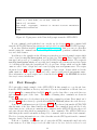
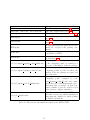
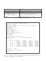
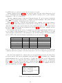
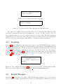
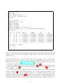

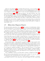
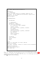

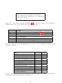
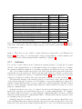
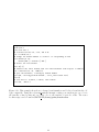
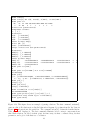
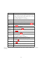
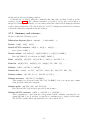
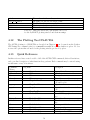
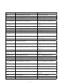
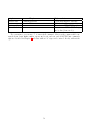
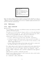


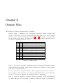

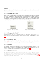
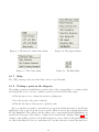

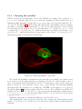
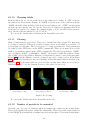
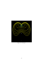
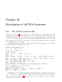


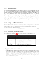
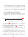
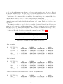
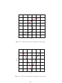
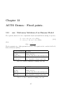
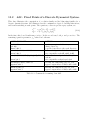
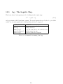
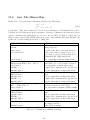

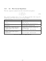
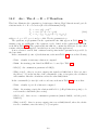
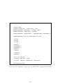
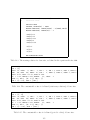
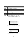
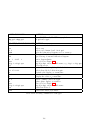
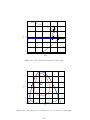
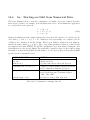
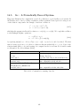
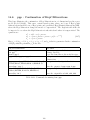
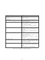
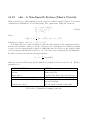
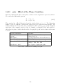
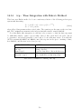
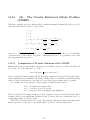
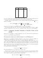


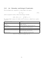
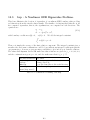
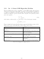
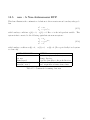
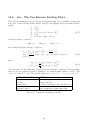
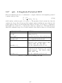
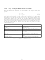
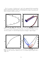
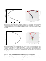
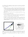
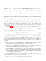
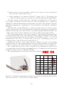
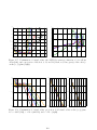


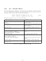
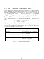
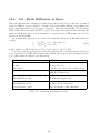
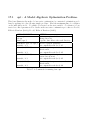
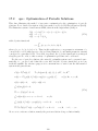

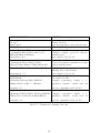
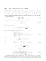


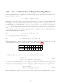
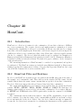

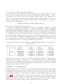
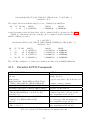
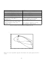
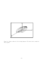
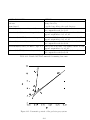
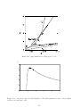
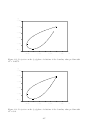

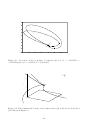
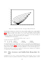
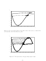
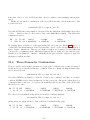
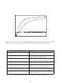
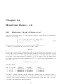
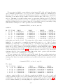

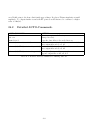
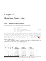

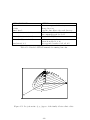
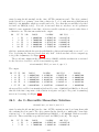
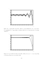
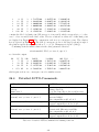
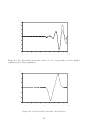
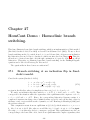
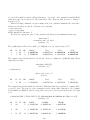
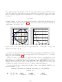
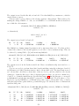
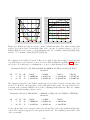
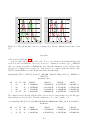
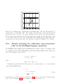
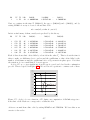
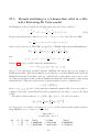

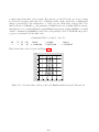


![[1 ] Oracle® Fusion Middleware](http://vs1.manualzilla.com/store/data/005867961_1-9a6cb85523fc7e3a2bcbfd437b088639-150x150.png)