Download Toupie User's Manual

Toupie User's Manual
Marc-Michel Corsini and Antoine Rauzy
Contents
1 Introduction
2 How To Run Toupie
2.1
2.2
2.3
2.4
2.5
2.6
2.7
Getting Started : : : : : : : : : : : :
Reading Programs : : : : : : : : : :
Inserting De nitions at the Terminal
Directives: Queries and Commands :
Syntax Errors : : : : : : : : : : : : :
Exiting from the Interperter : : : : :
Saving and Restoring a Program : :
:
:
:
:
:
:
:
:
:
:
:
:
:
:
:
:
:
:
:
:
:
:
:
:
:
:
:
:
:
:
:
:
:
:
:
:
:
:
:
:
:
:
:
:
:
:
:
:
:
:
:
:
:
:
:
:
:
:
:
:
:
:
:
:
:
:
:
:
:
:
:
:
:
:
:
:
:
:
:
:
:
:
:
:
:
:
:
:
:
:
:
:
:
:
:
:
:
:
:
:
:
:
:
:
:
:
:
:
:
:
:
:
:
:
:
:
:
:
:
:
:
:
:
:
:
:
:
:
:
:
:
:
:
:
:
:
:
:
:
:
:
:
:
:
:
:
:
:
:
:
:
:
:
:
:
:
:
:
:
:
:
:
:
:
:
:
:
:
:
:
:
:
:
:
:
3 Commands
:
:
:
:
:
:
:
3.1 Commands : : : : : : : : : : : : : : : : : : : : : : : : : : : : : : : : : : : : : : : :
3.2 Display Commands : : : : : : : : : : : : : : : : : : : : : : : : : : : : : : : : : : : :
4 The Toupie Language
4.1 Syntax : : : : : : : : : : : :
4.1.1 Terms : : : : : : : :
4.1.2 Formulae : : : : : :
4.1.3 Fixpoint De nitions
4.1.4 Additional Features
4.2 Semantics : : : : : : : : : :
:
:
:
:
:
:
:
:
:
:
:
:
:
:
:
:
:
:
:
:
:
:
:
:
:
:
:
:
:
:
:
:
:
:
:
:
:
:
:
:
:
:
:
:
:
:
:
:
:
:
:
:
:
:
:
:
:
:
:
:
:
:
:
:
:
:
:
:
:
:
:
:
:
:
:
:
:
:
:
:
:
:
:
:
:
:
:
:
:
:
:
:
:
:
:
:
:
:
:
:
:
:
:
:
:
:
:
:
:
:
:
:
:
:
:
:
:
:
:
:
:
:
:
:
:
:
:
:
:
:
:
:
:
:
:
:
:
:
:
:
:
:
:
:
:
:
:
:
:
:
:
:
:
:
:
:
:
:
:
:
:
:
:
:
:
:
:
:
:
:
:
:
:
:
:
:
:
:
:
:
2
3
3
3
4
4
4
4
4
5
5
6
8
: 8
: 8
: 9
: 9
: 9
: 10
5 Programming Examples
13
A Syntax
B Reported Bugs
20
22
5.1 The Wolf, the Goat and the Cabbage : : : : : : : : : : : : : : : : : : : : : : : : : : 13
5.2 Nim Game : : : : : : : : : : : : : : : : : : : : : : : : : : : : : : : : : : : : : : : : 14
5.3 Milner's scheduler : : : : : : : : : : : : : : : : : : : : : : : : : : : : : : : : : : : : 16
1
Chapter 1
Introduction
Toupie is a -calculus interpreter in which variables take their values in (symbolic) nite domains.
Toupie uses decision diagrams (an extension to nite domains of Bryant's Binary Decision Diagrams [Bry86, BRB90, Bry92]) to encode formulae and relations. Initially, Toupie was designed to
perform abstract interpretation of Prolog programs [CMR92]. The current version has a wide spectrum of applications, including model checking [CGR93], static analysis of declarative languages
[CCMR93], and resolution of classical Arti cial Intelligence puzzles.
This manual describes the version 0.24 of Toupie, developed at the Laboratoire Bordelais de
Recherches en Informatique (LaBRI). The system is written in standard ANSI C and can thus
run on many platforms (SUN Spark Station, IBM RISC 6000, PC linux, Apple Macintosh, Next
Station), provided that there exist minimal ressources such as a video screen with termcap entry.
The user interface of Toupie is a small command interpreter. These commands permit the
loading, observation and deletion of programs; as well as interactive queries and responses.
From a more theoretical point of view, there are many papers devoted to the (propositional)
-calculus. But, since the syntax and the semantics we have adopted do not follow these usual
presentations, we have tried to make this manual as self-contained as possible.
Remarks, comments are welcome:
Antoine Rauzy
LaBRI { URA CNRS 1304 { Universite Bordeaux I
33405 Talence cedex { FRANCE
tel: (33) 56 84 60 83, fax: (33) 56 84 66 69
e-mail: [email protected]
2
Chapter 2
How To Run Toupie
Toupie o ers the user an interactive programming environment for incrementally building programs.
The text of a Toupie program is normally created in a le (or a number of les) using a standard
text editor. The Toupie interpreter can be instructed to read programs from these les.
2.1 Getting Started
Toupie is typically started from one of the UNIX shells by entering the command
% toupie
The interpreter responds with a banner message and the prompt `2p
to accept input; thus:
|='
as soon as it is ready
--- Toupie version 0.24 (04/10/93)
Antoine Rauzy
LaBRI - URA CNRS 1304 - Universite Bordeaux I
351, cours de la Liberation - 33405 Talence - France
[email protected]
2p |=
2.2 Reading Programs
A program consists of a sequence of domain and xpoint de nitions, possibly interspersed with directives to the interpreter. The order between xpoint de nitions has no importance, but domains
must be declared before their use.
To input a program from a le file, type the command:
2p |= load file
Note that it is not necessary to surround the le name with any additional symbols. Thus, the
following command is legal:
2p |= load Benchmarks/Queens/queens8.2p
We use to adopt the extension \.2p" for les containing Toupie programs. Nevertheless, this
extension is not implicitely added nor required.
Warning: in the current version, if a xpoint equation is de ned more than once, all versions
are maintained. It may result an unexpected behavior.
3
CHAPTER 2. HOW TO RUN TOUPIE
4
2.3 Inserting De nitions at the Terminal
Domains and xpoint de nitions may also be typed directly at the terminal, although this is not
recommended since the syntax is suciently complicated to induce many typographical errors. To
enter a de nition at the terminal, it suces to type it. E.g. a domain de nition:
2p |= let my_domain {a, b, c, d}
A xpoint de nition (predicate p):
2p |= p(X:my_domain,Y:my_domain) += (X#Y)
For the precise syntax of Toupie formulae and programs see Chap. 4.
2.4 Directives: Queries and Commands
Directives are either queries or commands. The full syntax of a query is a formula followed by a
question mark ?, e.g.
2p |= (X:{a,b,c} = Y:{d,c,b}) ?
This query contains two variables X and Y that belong respectively to the sets of symbolic
constants fa; b; cg and fd; c; bg. It looks for the pairs < v; w > of possible values of X and Y , such
that v = w.
If the query speci ed admits solutions (as in the previous example), the system answers:
{X=b, Y=b}
{X=c, Y=c}
meaning that there are two pairs of values that verify the equality. The execution of the query
then terminates.
If all the possible assignments of the variables occurring in the query are solutions (e.g.
(X:{a,b}=X) ?), the system answers 1. If none of these assignments is solution (e.g. (X:1..3#X) ?)
the system answers 0.
2.5 Syntax Errors
Syntax errors are detected during reading. If an error occurs when reading a de nition or a
directive, a message is printed indicating at which line the error has been detected. E.g.
2p |= (X=Y) ?
2p ->
line 1: the variable X hasn't a domain.
Normally, no de nition is stored and you can return to the interpreter by typing RETURN
twice.
2.6 Exiting from the Interperter
To exit from the interpreter and return to the shell level, type a ^C or a ^D (UNIX interrupts), or
use the command exit.
2.7 Saving and Restoring a Program
In order to suppress all of the de nitions that are currently stored, use the command clear all.
These de nitions can be saved into a text le by means of the command save followed by a le
name (as in the command load).
Chapter 3
Commands
This chapter describes the commands of the Toupie interface.
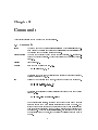
3.1 Commands
clear
dependencies
display
domain
This command has two options: clear program which reinitializes the program (all the de nitions are deleted); and clear all which reinitializes both
the program and the decision diagrams manager.
Compute the dependency graph of each xpoint de nition, i.e. the links between the xpoint de nitions. These dependencies can be displayed (see Section 3.2).
(see Section 3.2).
used to de ne a default domain. E.g.
2p |= domain {a, b, c}
let
Thereafter, if the domain of a variable is not speci ed at its rst appearance,
it is set by default to fa; b; cg.
Followed by an identi er and a domain, de nes a domain of the given name.
2p |= let a_name { a, b, c }
2p |= let another_name 1..4
Thereafter, it is possible to declare variables that belong to domain by giving
its name. E.g.
2p |= (X:a_name = Y:another_name) ?
For implementation reasons, it is far more ecient to use named domains
rather to repeat them when several variables have the same domain. The
syntax of domain names is the same as the syntax of symbolic constants (and
thus it is highly discouraged to use the same identi er as a constant and a
domain name). Note that in let name domain, domain cannot be the name
of a previously de ned domain, and that it is not possible to rede ne a named
domain.
5
CHAPTER 3. COMMANDS
6
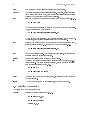
exit
garbage
load
Terminates the Toupie cession and returns to control monitor.
The Decision Diagrams garbage collector is called. Normally, it is not necessary
for the user to call this command, since the garbage collection is automatically
performed when there is not enough space available.
followed by a le name file: inputs a program from the given le file. E.g.
2p |= load file
Note that it is not necessary to surround the le name with any delimiters.
Thus, the following command is legal:
2p |= load Benchmarks/Queens/queens8.2p
save
We use to adopt the extension \.2p" for les containing Toupie programs.
Nevertheless, this extension is not implicitely added nor required.
Followed with a le name (with the same syntax that for the load command),
saves the current program (i.e. domains and xpoint de nitions). E.g.
2p |= save Benchmarks/Queens/queens8.2p
stat
nostat
spy
Turn on the statistic option. As the result (in this version), the running time
is printed after each request computation.
Turn o the statistic option (this is the default value).
This command takes two arguments: a predicate name and its arity, i.e. a
positive integer. The spied predicate is traced, that is a message is printed
each time its value is recomputed. E.g.
2p |= spy p 2
2p -> predicate p/2 spied
nospy
system
This command has the same syntax as spy. It disactives the spy option for
the given predicate.
A UNIX command is read on the current line, and is then executed.
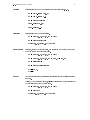
3.2 Display Commands
The display command takes an argument:
domain
Displays the current default domain. E.g.
2p |= domain {a,b,c}
2p |= display domain
domain {a,b,c}
3.2. DISPLAY COMMANDS
domains
7
Displays all of the named domains together with their values. E.g.
2p |= let a_domain {a,b,c}
2p |= let b_domain 1..4
2p |= display domains
let a_domain {a,b,c}
let b_domain 1..4
equations
Displays all of the xpoint equations.
2p |= p(X:{a,b,c},Y:{d,c,b}) += (X=Y)
2p |= display equations
p(X@1:{a,b,c},Y@2:{d,c,b}) += (X=Y)
dependencies
Displays, for each xpoint equation, the predicates that must be recomputed
when the de ned one changes of value.
2p |= p(X:{a,b,c},Y:{d,c,b}) += (X=Y)
2p |= q(X:{a,b,c},Y:{d,c,b}) += (p(X,Y) | q(Y,X))
2p |= dependencies
2p |= display dependencies
p/2 --> q/2,
q/2 -->
memory
For debugging purpose only: displays the current state of the decision diagrams
manager.
Followed by an predicate identi er, display displays the xpoint de nitions of
the predicates that have the given name.
2p |= p(X:{a,b,c},Y:{d,c,b}) += (X=Y)
2p |= display p
p(X@1:{a,b,c},Y@2:{d,c,b}) += (X=Y)
Chapter 4
The Toupie Language
This chapter provides a brief introduction to the syntax and semantics of Toupie programs.
4.1 Syntax
There are three syntactic categories in Toupie: terms, formulae and predicate de nitions. A Toupie
program is a set of predicate de nitions having di erent head predicate symbols or distinct arities.
A Toupie query is a formula.
4.1.1 Terms
The data objects of Toupie are called terms. A term is either a constant, a domain or a variable.
Constants:
The constant symbols are:
The positive integers such as 0, 1, 999. Note that arithmetical operations are not supported
in the current version.
The symbolic constants, that is any identi er in [a::z ][a::zA::Z 0::9 ]? (e.g., aConstant,
the 9th constant, : : : ).
Domains:
A set of constants is called a domain. There are two kinds of domains:
Ranges, written i::j , where i and j are positive integers such that i < j .
Sets, written fk1; : : :kr g, where the ki 's are constants.
It is possible to give a name to a domain, e.g.
2p |= let a_name { a, b, c }
For implementation reasons, it is far more ecient to use named domains, when several variables have the same domain. The syntax of domain names is the same than the syntax of symbolic
constants (and thus it is highly recommended to do not use the same identi er as a constant and
a domain name).
It might be the case that all the variables of a program belong to the same domain. A default
domain can be de ned, e.g.
2p |= domain {a, b, c}
Then, it is possible to declare a variable without specifying its domain; the variable then
belongs to the default domain.
8
4.1. SYNTAX
9
Variables:
The variable symbols are identi ers in[A::Z ][a::zA::Z 0::9 ]? (e.g., The 9th variable, Avariable,
: : : ).
Each variable occurring in a Toupie expression must have an interpretation domain. This
domain must be declared with the rst occurrence of the variable. A domain declaration for the
variable X is of the form: X : domain, where domain is any domain, included a domain name. In
this case, the domain must has been declared before.
Variables in di erent xpoint de nitions or requests are completely independent, even if they
have the same name | the lexical scope of a variable is limited to a single xpoint de nition or
request.
4.1.2 Formulae
Formulae have the following form:
The two Boolean constants 0 and 1.
(X1=X2) or (X1=k) or (X1#X2) or (X1#k) where X1 and X2 are variables and k is a constant
symbol.
(X in domain) where X is a variable and domain is any domain, including a domain name.
In this case, the domain must has been declared before.
P(X1,..., Xn) where P is an n-ary predicate variable and X1,: : : ,Xn are individual variables.
~ f, (f & g), (f | g), (f <=> g), (f <#> g), (f => g) where f and g are formulae
and ~, &, |, <=>, <#>, => denote the logical connectives :; ^; _; (); and ). Note
that the parentheses are absolutely required.
@(i,[f1,...,fn]), where i is positive integer and f1 ... fn are formulae. This connective is satis ed if and only if at least i 's are satis ed.
#(i,j,[f1,...,fn]), where i and j are positive integers and f1...fn are formulae. This
connective is satis ed i at least i and at most j 's are satis ed.
forall X1,..., Xn f or exist X1,..., Xn f where X1,: : : ,Xn are variables and f is a
formula. forall and exist denote respectively the two quanti ers 8 and 9.
4.1.3 Fixpoint De nitions
Predicate de nitions are as follows:
P(X1,...,Xn) += f
P(X1,...,Xn) -= f
where P is an n-ary predicate variable, X1,: : : ,Xn are individual variables, and f is a formula.
The token += and -= denote respectively least and greatest xpoint de nitions. The formula f is
assumed to be monotonic. This property can been easily checked by a syntactic inspection of the
formulae, but is NOT veri ed in the current version.
4.1.4 Additional Features
Comments
It is possible to have comments in a Toupie program. A % indicates that the text between this
symbol and the end of the line is a comment.
CHAPTER 4. THE TOUPIE LANGUAGE
10
Variable Ordering
The internal data structures of Toupie, namely the Decision Diagrams (for a more technical presentation of Toupie see [CR93a, CR93b]), require an order over the variables of a xpoint de nition
or a formula. By default, the variables are ordered by their order of appearance.
It is often necessary, for sake of eciency, to customize this order. An index can be thus
declared with the rst occurrence of the variable, with the following syntax: X@i where i is a
positive integer. E.g.
let vertex 1..10
edge(X:vertex, Y:vertex) += (
% relation that defines a graph
...
)
closure(X@1:vertex,Y@3:vertex) += (
edge(X,Y)
| exist Z@2:vertex (edge(X,Z) & closure(Z,Y))
)
If an unindexed variable occurs in a formula, its index is the integer that follows immediately
the greatest de ned index.
4.2 Semantics
The semantics of Toupie formulae is determined with respect to a structure S = hConst ; Vi where
Const is an interpretation domain, and V is a denumerable set of variables including all the
variables of the program. As in DATALOG, we assume, rst, the hypothesis of unicity of names
(two distinct constant symbols denotes two distinct constants), and second, the hypothesis of the
closure of the domain, that is to say that Const is the set of all the constants occurring in the
considered formula or program.
De nition 1 [Individual Variable Assignments]
An individual variable assignment is a mapping from V into Const such that (X ) 2 dom(X )
for any variable X occurring in the program.
For sake of simplicity, we assume implicitely the condition (X ) 2 dom(X ).
De nition 2 [Relations]
A relation on S is a mapping from V ! Const into B, where X ! Y stands for the set of mappings
from X to Y and B stands for the Boolean values.
De nition 3 [Predicate Variable Interpretations]
Let Pr be the set of predicates occurring in the program. A predicate variable interpretation is a
mapping from Pr into (IN ! Const ) ! B, where IN stands for the set of natural numbers.
This de nition avoids the complications due to the di erent arities of the predicates. For a
predicate of arity n, it suces to consider that the corresponding function depends only on the
rst n numbers.
The semantics of a formula is thus a relation, and the semantics of a predicate (de ned with
a xpoint equation) is a mapping from (IN ! Const ) into B.
A Toupie program P assigns a meaning to a set of predicate symbols Pr. The semantics
of the program is de ned as the least xpoint of a transformation T . Let us denote by PR
4.2. SEMANTICS
11
the set Pr ! (IN ! Const ) ! B of predicate variable interpretations, and by RE the set
(V ! Const ) ! B of relations.
The program de nes a continuous transformation:
T : PR ! PR
Each formula f de nes a function:
T [ f] : PR ! RE
And each equation Eq de nes a function:
T [ Eq] : PR ! (IN ! Const ) ! B
The de nition of T will use the following notation.
De nition 4 [Substitutions]
Let f : A ! B be a function. Let a1 ; : : :; an be distinct elements of A, and b1; : : :; bn be arbitrary
elements of B . We note by
f [a1 =b1 ; : : :; an=bn]
the function g : A ! B such that gai = bi (1 i n) and ga = fa (8a 62 fa1; : : :; ang).
The notation
[a1=b1; : : :; an=bn]
stands for f [a1 =b1; : : :; an=bn] where f is an arbitrary function.
We are now in position to de ne the semantic function T . Let be a predicate variable
interpretation, be an individual variable assignment, and be an element of (IN ! Const ). T
is de ned inductively on the structure of formulae in the following way :
T [ 1]] = 1 and T [ 0]] = 0:
T [ Xi = Xj ] = (Xi ) = (Xj ).
T [ Xi = k] = (Xi ) = k.
T [ g] = :T [ f ] .
T [ f j g] = T [ f ] _ T [ g] :
T [ f & g] = T [ f ] ^ T [ g] :
V
T [ 8 X f ] = k dom(X ) (T [ f ] [X=k]):
T [ 9 X f ] = Wk dom(X ) (T [ f ] [X=k]).
T [ P (Xi1 ; : : :; Xir )]] =(P )( (Xi1 ); : : :; (Xir )).
T [ P (X1; : : :; Xn )+ = f ] =T [ f ] [X1=(1); : : :; Xn =(n)].
Finally, the transformation associated with the program is:
T [ Eq1 : : :Eqn] = [p1=T [ Eq1] ; : : :; pn=T [ Eqn] ]
where the pi are the predicates de ned by the equations Eqi.
De nition 5 [Denotation of a Toupie Formula wrt. a Program]
Let P be a Toupie program. Let f be a Toupie formula. Let D be the set of free variables occurring
in f . By de nition, the denotation of f wrt. P is the function D[ f ] : (D ! Const ) ! B such
that, for all 2 (D ! Const ),
D[ f ] = T [ f ] ((T [ P ] )) ;
where is any variable assignment such that
X = X (8X 2 D):
(The underlying program remains implicit.)
2
2
0
0
0
12
CHAPTER 4. THE TOUPIE LANGUAGE
Note that the introduction of greatest xpoint de nitions complicates the notation but not the
semantics itself.
Chapter 5
Programming Examples
In this chapter, three examples are examined in details.
5.1 The Wolf, the Goat and the Cabbage
The rst problem we examine is the well-known boatman problem. The sad story is the following:
a poor old boatman wants to cross the river with his wolf, his goat and cabbage; alas his two-place
boat is too small for all of his belongings, the river is too deep to cross it by foot and the closest
bridge is far. He cannot leave the wolf alone with the goat nor the goat alone with the cabbage.
To solve it, one could try the following program:
% the boatman story
domain {left,right}
% default domain declaration
% reachable describes all of the possible states, i.e. all the
% possible positions of the man (M), the wolf (W), the goat (G)
% and the cabbage (C).
reachable(M,W,G,C) += (
% initial state: every one is on the left bank
((M=left) & (W=left) & (G=left) & (C=left))
| (
( % the possible crossings
(reachable(M2,W,G,C) & (M2#M))
%
| (reachable(M2,W2,G,C) & (M2=W2) & (M=W) & (M2#M)) %
| (reachable(M2,W,G2,C) & (M2=G2) & (M=G) & (M2#M)) %
| (reachable(M2,W,G,C2) & (M2=C2) & (M=C) & (M2#M) %
)
&
% Exclude the forbidden states
~(((W=G) | (G=C)) & (M#G))
)
)
man
man
man
man
alone
+ wolf
+ goat
+ cabbage
The set of accessible states is computed via xpoint, and the boatman reaches safely the other
bank with his goods since the call of reachable succeeds with the four arguments set to right:
2p |= reachable(Man,Wolf,Goat,Cabbage) ?
13
CHAPTER 5. PROGRAMMING EXAMPLES
14
{Man=left, Wolf=left, Goat=left}
{Man=left, Wolf=left, Goat=right, Cabbage=left}
{Man=left, Wolf=right, Goat=left}
{Man=right, Wolf=left, Goat=right}
{Man=right, Wolf=right, Goat=left, Cabbage=right}
{Man=right, Wolf=right, Goat=right}
2p |= reachable(right,right,right,right) ?
1
5.2 Nim Game
The Nim game has the following rules:
The game begins with N lines numbered from 1 to N and containing 2 i 1 matches. At
each step, the player who has the turn takes as many matches as he wants in one of the line (but of
course, at least one). Then the turn changes. The winner is the player who takes the last match.
In order to model this problem, one rst models each line by means of a nite state automaton,
itself encoded in Toupie as a ternary relation (initial state, transition label, terminal state). Note
that it is not necessary to model the turn explicitely since it changes of value alternatively.
The states of a line represent the number of matches it contains currently. For instance, the
line number 3 is modeled by means of a 3 states automaton (0,1,: : : 5 matches). The transition are
labelled either with e (the empty transition) or with c. The rst one means that the automaton
stays in the same state, the second one that the player who has the turn takes a number of matches
in this line.
For instance, for the line number 3, it gives:
let label {e,c}
% domain of transition labels
let state3 0..5
% domain of state of the line number 3
% The automaton for the line number 3
% S: initial state, L:label, T: terminal state of a transition
line3(S@7:state3,L@8:label,T@9:state3) += (
((L=e) & (S=T))
| ((S=1) & (L=c) & (T=0))
| ((S=2) & (L=c) & (T in 0..1))
| ((S=3) & (L=c) & (T in 0..2))
| ((S=4) & (L=c) & (T in 0..3))
| ((S=5) & (L=c) & (T in 0..4))
)
In the above program, one has de ned the variable indices. The reason is given below.
Now, one models the system compounded by the di erent lines. This system can be seen as
the product of the di erent automata. The states of the product are the N -tuples of states (a
state for each basic automaton) and its transitions are N -tuples of transitions. Of course, all the
tuples of transitions are not allowed, since the player who has the turn must take a number of
matches in one and only one line. The product is thus synchronized by means of the following
predicate (for 3 lines):
% one and only one line changes of state at each turn:
synchronizator(L1@2:label,L2@5:label,L3@8:label) += (
5.2. NIM GAME
15
((L1=c) & (L2=e) & (L3=e))
| ((L1=e) & (L2=c) & (L3=e))
| ((L1=e) & (L2=e) & (L3=c))
)
Now, the reachable states in the synchronized product are computed of two steps: the rst
one consists in computing all the allowed edges; the second one consists in computing all the
states reachable from the initial one, through allowed edges. It has been noted by several authors
[Bou93, CGR93, EFT93] that the best variable ordering for computing a synchronized product, is
the interleaved one (as de ned in the predicate edge). This is why this ordering has been choosen
for the automata description.
edge(S1@1:state1,T1@3:state1,S2@4:state2,T2@6:state2,S3@7:state3,T3@9:state3) +=
exist L1@2:label, L2@5:label, L3@8:label
(
line1(S1,L1,T1)
& line2(S2,L2,T2)
& line3(S3,L3,T3)
& synchronizator(L1,L2,L3)
)
reachable(T1@3:state1,T2@6:state2,T3@9:state3) += (
((T1=1) & (T2=3) & (T3=5)) % initial state
| exist S1@1:state1, S2@4:state2, S3@7:state3
(
reachable(S1,S2,S3)
& edge(S1,T1,S2,T2,S3,T3)
)
)
Now, one obtains the con gurations where there is a winning strategy by means of the two
following predicates:
winning(S1@1:state1,S2@4:state2,S3@7:state3) +=
exist T1@3:state1,T2@6:state2,T3@9:state3
(
edge(S1,T1,S2,T2,S3,T3)
& losing(T1,T2,T3)
)
losing(S1@1:state1,S2@4:state2,S3@7:state3) +=
forall T1@3:state1,T2@6:state2,T3@9:state3
(
edge(S1,T1,S2,T2,S3,T3)
=> winning(T1,T2,T3)
)
There exists at least one winning strategy for the rst player since one obtains:
2p |= winning(1,3,5) ?
1
CHAPTER 5. PROGRAMMING EXAMPLES
16
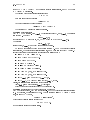
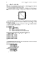
5.3 Milner's scheduler
This problem is a simple distributed scheduler proposed by Milner [Mil89]. It is now a standard
benchmark for process algebra tools [Bou93, EFT93].
The scheduler consists of one starter process and N processes which are scheduled. The
communication is organized in a ring. The transition system describing each cycler is depicted
below:
0
sc
6@@ rc
@@R
4
tau
3
6
1 a
@
tau
@@
@R
sc
2
Each cycler process Ci awaits the permit (rc) to start, performs the action a, and passes the
turn (sc) to the next cycler either before or after some internal computation (tau). The starter
just initializes the process.
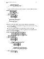
The system is programmed in the same way that the Nim game is. The cyclers are described
by means of the following ternary predicate:
let cycler_state 0..4
let cycler_label {e,tau,a,sc,rc}
% tau : internal action,
% a
: idem
% sc : send the starter to the next cycler
% rc : receive the starter from the previous cycler
cycler(S@4:cycler_state,L@5:cycler_label,T@6:cycler_state) += (
((L=e) & (S=T))
| ((S=0) & (L=rc) & (T=1))
| ((S=1) & (L=a)
& (T=2))
| ((S=2) & (L=sc) & (T=3))
| ((S=2) & (L=tau) & (T=4))
| ((S=3) & (L=tau) & (T=0))
| ((S=4) & (L=sc) & (T=0))
)
A synchronized product can be computed as in the previous section (we just give the predicate
for one starter and three cyclers.
reachable
reachable(TS@3:starter_state,
T1@6:cycler_state,
T2@9:cycler_state,
T3@12:cycler_state) += (
((TS=0)&(T1=0)&(T2=0)&(T3=0))
| exist SS@1:starter_state,
S1@4:cycler_state,
S2@7:cycler_state,
S3@10:cycler_state
(
5.3. MILNER'S SCHEDULER
17
reachable(SS,S1,S2,S3)
& edge(SS,TS,S1,T1,S2,T2,S3,T3)
)
)
Now, one can verify that there is no deadlock in the system by means of the following predicate:
deadlock(SS@1:starter_state,
S1@4:cycler_state,
S2@7:cycler_state,
S3@10:cycler_state) += (
reachable(SS,S1,S2,S3)
& forall TS@3:starter_state,
T1@6:cycler_state,
T2@9:cycler_state,
T3@12:cycler_state
(
edge(SS,TS,S1,T1,S2,T2,S3,T3)
=>
deadlock(TS,T1,T2,T3)
)
)
Finally one computes a bisimulation on this example that consists of the following steps:
1. Compute the -closure of the synchronized product, that is the paths of the form ? t ? ,
where t is any transition.
2. Compute the equivalence relation between states using the extended edges above.
We just give hereafter the program for the second step, assuming that the rst step has been
performed by the predicate large_edge.
bisimulation(XT@1:starter_state,YT@3:starter_state,
X1@9:cycler_state,Y1@11:cycler_state,
X2@13:cycler_state,Y2@15:cycler_state,
X3@17:cycler_state,Y3@19:cycler_state) -= (
reachable(XT,X1,X2,X3)
& reachable(YT,Y1,Y2,Y3)
& forall UT@2:starter_state,
U1@10:cycler_state,
U2@14:cycler_state,
U3@18:cycler_state
(
large_edge(XT,UT,X1,U1,X2,U2,X3,U3)
=> exist VT@4:starter_state,
V1@12:cycler_state,
V2@16:cycler_state,
V3@20:cycler_state
(
large_edge(YT,VT,Y1,V1,Y2,V2,Y3,V3)
& bisimulation(UT,VT,U1,V1,U2,V2,U3,V3)
)
)
& forall VT@4:starter_state,
V1@12:cycler_state,
CHAPTER 5. PROGRAMMING EXAMPLES
18
V2@16:cycler_state,
V3@20:cycler_state
(
large_edge(YT,VT,Y1,V1,Y2,V2,Y3,V3)
=> exist UT@2:starter_state,
U1@10:cycler_state,
U2@14:cycler_state,
U3@18:cycler_state
(
large_edge(XT,UT,X1,U1,X2,U2,X3,U3)
& bisimulation(UT,VT,U1,V1,U2,V2,U3,V3)
)
)
)
Bibliography
[Bou93]
A. Bouali. Etudes et mises en uvre d'outils de veri cation basee sur la bisimulation.
PhD thesis, Universite Paris VII, 03 1993. in french.
[BRB90] K. Brace, R. Rudell, and R. Bryant. Ecient Implementation of a BDD Package. In
27th ACM/IEEE Design Automation Conference. IEEE 0738, 1990.
[Bry86] R. Bryant. Graph Based Algorithms for Boolean Function Manipulation. IEEE Transactions on Computers, 35:677{691, 8 1986.
[Bry92] R. Bryant. Symbolic Boolean Manipulation with Ordered Binary-Decision Diagrams.
ACM Computing Surveys, 24(3):293{318, September 1992.
[CCMR93] M-M. Corsini, B. Le Charlier, K. Musumbu, and A. Rauzy. Ecient Abstract Interpretation of Prolog Programs by means of Constraint Solving over Finite Domains
(extended abstract). In Proceedings of the 5th Int. Symposium on Programming Language Implementation and Logic Programming, PLILP'93, Estonie, 1993.
[CGR93] M-M. Corsini, A. Gri ault, and A. Rauzy. Yet another Application for Toupie: Veri cation of Mutual Exclusion Algorithms. In proceedings of Logic Programming and
Automated Reasonning, LPAR'93. LNCS, 1993.
[CMR92] M-M. Corsini, K. Musumbu, and A. Rauzy. The -calculus over Finite Domains as an
Abstract Semantics of Prolog. In M. Billaud, P. Casteran, M-M. Corsini, K. Musumbu,
and A. Rauzy, editors, WSA'92 Workshop on Static Analysis (Bordeaux), volume 81{
82 of Bigre, pages 51{59. Atelier Irisa, Sept. 23{25 1992.
[CR93a] M-M. Corsini and A. Rauzy. First Experiments with Toupie. Technical Report 577{93,
LaBRI - Universite Bordeaux I, 1993.
[CR93b] M-M. Corsini and A. Rauzy. Toupie: the -calculus as a Constraint Language, 1993.
submitted to the Journal of Automated Reasonning.
[EFT93] R. Enders, T. Filkorn, and D. Taubner. Generating bdds for symbolic model checking
in ccs. Journal of Distributed Computing, 6:155{164, 6 1993.
[Mil89] R. Milner. Communication and Concurrency. Prentice Hall, New York, 1989.
19
Appendix A
Syntax
This appendix recalls the syntax of Toupie programs and requests in Bacchus Normal Form.
<request> ::= <fixed-point-or-request>
::= <formula> ?
<fixed-point-or-request> ::= <predicate> += <formula>
::= <predicate> -= <formula>
::= <predicate> ?
<formula> ::=
::=
::=
::=
::=
::=
::=
::=
<parenthesed-formula>
<projection>
<cardinality>
<at-least>
<quantifier>
<not>
<boolean-constant>
<predicate>
parenthesed-formula> ::= ( <atomic-relation> )
::= ( <composed-formula> )
<composed-formula> ::= <n-ary-connective>
::= <binary-connective>
::= <formula>
<binary-connective> ::= <formula> => <formula>
::= <formula> <=> <formula>
::= <formula> <#> <formula>
<n-ary-connective> ::= <item-list[ <formula>
::= <item-list[ <formula>
| ]>
& ]>
<predicate> ::= <identifier> ( item-list[ <argument> , ] )
<not> ::= ~ <formula>
<boolean-constant> ::= 0 | 1
<atomic-relation> ::= <variable> = <variable>
20
21
::=
::=
::=
::=
<variable>
<variable>
<variable>
<variable>
# <variable>
= <constant>
# <constant>
in <domain>
<quantifier> ::= exist <variables-list> <formula>
::= forall <variables-list> <formula>
<at-least> ::= @(<integer>, [ <item-list[ <formula> , ]> ])
<cardinality> ::= #(<integer>, <maximum>, [<item-list[<formula> ,]>])
<projection> ::= [ <formula>; <assignment-list> ]
<assignment-list> ::= <variable> <- <argument> , <assignment-list>
::= <variable> <- <argument>
<item-list[ <item> <separator> ]>
::= <item> <separator> <item-list[ <item> <separator> ]>
::= <item>
<argument> ::= <constant> | <domain> | <variable>
<domain> ::= <constant-set> | <range> | <functor>
<constant-set> ::= { <item-list [ <constant> , ]> }
<range> ::= <integer>..<integer>
<constant> ::= <integer> | <identifier>
<identifier> ::= any string of alphanum or _ letters beginning with
a lower case letter.
<variable> ::= any string of alphanum or _ letters beginning with
a lower case letter.
Appendix B
Reported Bugs
This appendix contains some bugs xed in the version 0.24.
If a constant is repeated in a domain de nition, no error nor warning message is printed.
E.g.
2p |= let a_domain {a, a, a}
2p |= (X:a_domain = Y: a_domain) ?
{X=a, Y=a}
{X=a, Y=a}
{X=a, Y=a}
If a xpoint equation is de ned twice, the two versions are maintained. It may result an
unexpected behavior.
2p |= let dom {a,b}
2p |= p(X:dom,Y:dom) += (X=Y)
2p |= p(X:dom,Y:dom) += (X#Y)
2p |= p(X:dom,Y:dom) ?
{X=a, Y=a}
{X=b, Y=b}
A variable cannot be declared twice in a request or a xpoint de nition, even if it is declared
under the scope of a quanti er.
2p |= p(X:{a,b},Y:1..2) += (
exist Z:{a,b} (X=Z)
& exist Z:1..2 (Y=Z)
2p ->
line 3: the variable Z has been used with another domain.
22