Download UMD Global 250 meter Land Water Mask User Guide 1

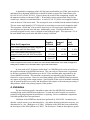
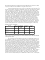
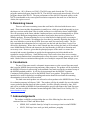
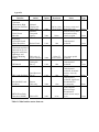
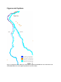
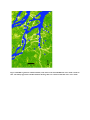
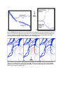
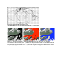
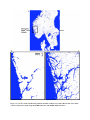
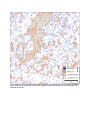
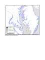
UMD Global 250 meter Land Water Mask User Guide
Mark Carroll, Charlene DiMiceli, John Townshend, Praveen Noojipady, Robert Sohlberg
1. Introduction
The new 250m land/water mask was created in three sections using primarily 3
different data sources. The main body of the product from 60° S to 60° N was created
using the SRTM Water Body Dataset (SWBD, 2005) and supplementing with MODIS
250m data as necessary. The area between 60° and 90° N was generated completely
from MODIS 250m data. While the area covering Antarctica between 60° and 90° S was
generated using the Mosaic of Antarctica product.
The SWBD was used because of its fine spatial resolution and because of its
consistent representation of the land surface. Since the SRTM data was collected over a
short time step, 11 days, it will provide a spatially coherent representation of surface
water. Additionally, the cloud penetrating properties of the RADAR offers superior
performance over spectral data alone, particularly in cloudy areas such as the humid
tropics. Using this remotely sensed data product has the advantage of a single source of
information, unlike the vector data sets which are dependent on disparate sets of
information to create a single data set.
The SWBD represents a significant improvement in the representation of land and
water. Unfortunately, a variety of problems remain with this data set. Foremost is
coverage, since it extends only from 55° S to 60° N. In the south this omits Antarctica,
and in the north this omits most of Alaska, the northern parts of Canada, Europe, and
Asia, as well as Greenland. In addition, the SWBD was created as ArcView shapefiles in
Geographic projection and subsetted into 1° squares. This format is acceptable for local
or small regional studies, but is cumbersome for doing large area studies. Note that there
are over 12,300 individual files necessary to get the full coverage of land surface for the
SWBD. If one tries to stitch together a large number of these (enough to make a single
MODIS tile, for example), in most cases the software (ARCGIS 9) will crash because of
the daunting number of individual shapes. In addition, despite best efforts there are still
data gaps in the SWBD. These gaps can occur when there are mid-stream islands and/or
where cloud cover was persistent. (pers. comm. James Slater (SWBD team) April 11,
2006) An attempt was made by the SWBD team to use the Landsat Geocover data to fill
these gaps, but gaps remain where the Geocover data was also too cloudy to make a
determination.
A global 250m data set in 16 day composites for the entire 8+ years of Terra data
and 6+ years of Aqua data, Collection 5, is online at the University of Maryland. This
data set (MOD44C) was originally created as the input to the MOD44A (Vegetative
Cover Conversion) and MOD44B (Vegetation Continuous Fields) products. For a full
description of this products see Carroll et al 2006. During the compositing process the
daily surface reflectance data (Vermote and Kotchenova, 2008) was interrogated using a
decision tree algorithm to distinguish between water and land. This daily depiction of
water was stored in the composite data as a sum of “hits” labeled as water in the process.
These “hits” were then interrogated and used where ever gaps exist in the SWBD.
The MODIS mosaic of Antarctica (MOA), available from the NSIDC DAAC, is a
mosaic of MODIS 250m level 1b (L1B) data for the continent of Antarctica. (Haran et al,
2005) This was generated using the Radarsat Antarctic Mapping Project Antarctic
Mapping Mission 1 (RAMP AMM1) data as a reference to overlapping MODIS
observations to create a fine resolution (125m) image for the continent of Antarctica. We
anticipate the release of a vector shoreline of Antarctica from this data set in February,
2007. When this is released it will be evaluated as a replacement for the existing 1km
product for Antarctica.
All data sets used here are available free of charge from various websites and
have either been published or used in products that have appeared in peer reviewed
publications. (see acknowledgements for access information)
2. Methods
2.1 60° S to 60° N
Initially, the SWBD was reprojected to MODIS Sinusoidal projection, converted
from vector to raster and stitched into MODIS tiles at the native 90m spatial resolution.
These 90m resolution tiles were aggregated to 250m resolution by absolute averaging to
yield percent water content per pixel. The projection from the native Geographic
projection to Sinusoidal projection can result in a loss of locational precision with
increasing latitude. However the conversion from vector to raster and subsequent
aggregation from 90m resolution to 250m resolution was sufficient to minimize any
discrepancies due to loss of precision with latitude.
Gaps in the SWBD derived 250m map were detected and filled in an automated
way using the methodology shown in Table 1.
•
•
•
Use the SWBD converted to raster and subset into MODIS tiles as the base mask
Group areas of contiguous water pixels into discrete water bodies
Create a reference map using 1 year of 250m daily water and land "hits"
o From the MOD44C composites for a year, compute the sum of land "hits"
and the sum of water "hits"
o Those pixels with at least 100 total observations and greater than 75%
water "hits" are considered water
• Working within a 10 x 10 pixel kernel
o Search for discrete water bodies that terminate within the kernel
o If found use the reference map to find suitable observations to connect the
water bodies
o Constraint: if the total number of water pixels in the kernel before adding
from the reference exceeds 20 (there are 100 pixels in a 10x10 kernel) do
not try to connect
ƒ This constraint helps avoid problems of connecting lakes
Table 1 Description of gap detection and filling algorithm
The SWBD did not provide coverage between 55° S to 60°S, however there is
essentially no land surface in this area. There are a total of 6 MODIS tiles that are
produced to have land in them in this range and it was found that there was only 1 island
not included in the SWBD in 1 tile. This island was mapped using MODIS 250m data.
2.2 60° to 90° N
MOD44C 250m 16-day composites are also available for areas between 60° and
90° N where the SWBD is not available. These data were used to create a new 250m
resolution land/water mask. The data were classified using regression tree classification
(Breiman et al, 1984). Training data were derived using the aggregated SWBD using a
tile in the MODIS v03 tile row (50° to 60° N) and the tree was applied to tiles in rows
v01 and v02 geographically nearby. A total of 3 different trees were used 1 in North
America, 1 in Europe, and 1 in Russia. Different trees were used in different geographic
locations to accommodate locally different ground cover to maximize the efficiency of
the tree. The regression trees were applied to multiple time periods and the resulting
classifications were averaged to increase the confidence that features were mapped
correctly.
The regression tree yields a subpixel estimate of the water component of a pixel.
Features were determined to be water bodies if the averaged classification result showed
50% or greater water content. This threshold is consistent with the threshold used to
determine water using the averaged SWBD data for regions between 60° S to 60° N.
2.2.1 80° to 90° N
Tiles in row v00 (80° to 90° N) were handled separately because most of the
water in this area remains frozen even in summer due to the high latitude and in some
cases there are ice shelves that extend from the land to the ocean. In the MODIS tile grid
there are only 4 tiles in this region which contain land. Because of the small number of
tiles and the complex landscape an inverse mapping approach was adopted whereby
water was determined by first mapping the visible land, and the area outside the
projection. The remaining area was initially labeled as water and was reclassified as land
if it could be determined that it was indeed ice over land.
This was accomplished by creating a decision tree with 3 classes land, ice and
water and applying it to the 4 16-day composites that comprise July and August for 5
years from 2003 - 2007. The information from 2003 – 2007 was combined to yield a
single static map for each of the 4 tiles. The EOS DEM for MODIS contains the old
water mask and was found to have substantial locational shifts which made it unsuitable
to use in determining elevation. For this reason interior ice sheets were digitized because
no other consistent DEM product was found to determine elevation. The NSIDC 1km
DEM for Greenland was used in the area of the McKinley Sea in the Northeastern corner
of Greenland due to the existence of an ice shelf.
2.3 60° to 90° S
The MOA grounding line vector data set has been reprojected from Polar
Stereographic to Sinusoidal, converted from vector to raster and subset into MODIS tiles.
The polyline shapefile was converted to a polygon and rasterized such that any data
inside the polygon was considered land and anything outside the polygon is considered
water. This reformatted product is included in the beta release of the new 250m water
mask as the land water mask for Antarctica. The grounding line is the point at which the
ice sheet is still resting on solid rock. (Scambos et al, 2007) The cryospheric community
has used this reference in their products for a number of years.
2.4 Quality Assurance Data Layer
A QA layer was maintained that shows which data source provided the water
pixel. For example, the area seen in red in figure 4 has a value that is distinct from the
area shown in blue designating that it came from a different source (in this case MODIS).
Users can utilize this layer to determine the utility of the data. Success was determined
by overlaying the new water mask with current MODIS surface reflectance data (multiday composites) to discover any gross errors of commission. Additionally, we will
release a beta version early in the project in order to incorporate user feedback into the
quality control process by investigating areas identified by end users as problematic.
3. Product Details
The new 250m water mask is a global raster data set in the Sinusoidal projection,
subset into tiles matching the MODIS tile grid. There are 3 discrete values represented:
•
0
Land
•
1
Water
•
253
Fill (outside the projection)
This dataset is intended to replace the old EOS 1km Land/Water mask originally created
in the mid-1990’s and updated in 2002. The 2002 update was performed by Boston
University (Salomon et al, 200?) and solved numerous errors including many misplaced
rivers in South America. The update was, however, limited to available data and hence
no update was possible for 80° to 90° N because no appropriate MODIS data were
available to them at that time. Dramatic improvement is seen in this region in the new
250m water mask and represents an update to the original EOS Land/Water mask from
the 1990’s.The UMD Global 250 meter Land Water Mask has been generated using data
from the Shuttle Radar Topography Mission (SRTM), MODIS data from Terra and Aqua
instruments, Landsat, and ASTER. The base product between 60 N and 60 S was the
SRTM Water Body Dataset (SWBD) which was converted from vector to raster 90m
spatial resolution, projected Sinusoidal projection and aggregated to 250m spatial
resolution. This data set was then subset into tiles using the MODIS tile grid and each
tile was visually inspected for obvious errors. Each tile was passed through a custom
algorithm which detects discontinuities in water bodies. Where discontinuities were
identified MODIS 250m data was used to fill in the discontinuity where appropriate.
Daily MODIS data was characterized for 3 years of data (2000 – 2003) to generate a
likelihood of water. Areas that were detected as discontinuous but showed a high
likelihood of water in MODIS were reclassified as water. For areas north of 60 N the
MODIS likelihood of water was used with some additional training and clarification
using Landsat and ASTER data.
Data sets Used
•
SRTM Water Body Dataset (SWBD) 2005. accessed July, 2005
•
MOD44C, 2008. (UMD internal data set)
•
Canadian Forest Service and Canadian Space Agency joint project Earth
Observation for Sustainable Development of Forests (EOSD) is the production of
a land cover map of the forested area of Canada
(http://www4.saforah.org/eosdlcp/nts_prov.html accessed Oct. 30, 2008)
•
NLCD2001 for Alaska (http://www.mrlc.gov/nlcd_multizone_map.php accessed
Jul. 21, 2008)
•
DiMarzio, J., A. Brenner, R. Schutz, C. A. Shuman, and H. J. Zwally. 2007.
GLAS/ICESat 1 km laser altimetry digital elevation model of Greenland. Boulder,
Colorado USA: National Snow and Ice Data Center. Digital media.
File format
File format is plain binary with 0 header bytes. The MODIS Sinusoidal tile grid
was used for compatibility with standard MODIS products. Spatial resolution is
231.65635m and each tile is square 4800x4800 pixels. A metadata file is associated with
each data file and contains georeferencing information as well as legend, production, and
citation information.
References
Breiman, L., Friedman, J. H., Olshen, R. A., & Stone, C. J. 1984. Classification and
regression trees. New York: Chapman & Hall.
Carroll, M., Townshend, J., Hansen, M., DiMiceli, C., Sohlberg, R., Wurster, K. (2006)
Vegetative Cover Conversion and Vegetation Continuous Fields. In
Ramachandran,, B., Justice, C.O., Abrams, M. (eds.) Land Remote Sensing and
Global Environmental Change: NASA’s Earth Observing System and the Science
of ASTER and MODIS Springer-Verlag (accepted).
DiMarzio, J., A. Brenner, R. Schutz, C. A. Shuman, and H. J. Zwally. 2007.
GLAS/ICESat 1 km laser altimetry digital elevation model of Greenland. Boulder,
Colorado USA: National Snow and Ice Data Center. Digital media.ESRI. 1992.
The Digital Chart of the World for use with ARC/INFO® Data Dictionary. ESRI,
Redlands, CA.
Haran, T., Bohlander, J., Scambos, T., Fahnestock, M. 2005. MODIS mosaic of
Antarctica (MOA) image map. Boulder, CO USA: National Snow and Ice Data
Center. Digital media
Justice, C., Giglio, L., Korontzi, S., Owens, J., Morisette, J., Roy, D., Descloitres, J.,
Alleaume, S., Petitcolin, F., and Kaufman, Y. 2002. The MODIS fire products,
Remote Sensing of Environment, 83(1&2), 244-262.
Lehner, B., and Doll, P., 2004. Development and validation of a global database of lakes,
reservoirs, and wetlands. Journal of Hydrology, 296, 1-22.
Salomon, J., Hodges, J., Friedl, M. Schaaf, C., Strahler, A., Gao, F., Schneider, A.,
Zhang, X., El Saleous, N., Wolfe, R. 200?. Global Land–Water Mask Derived
from MODIS Nadir BRDF–Adjusted Reflectances (NBAR) and the MODIS Land
Cover Algorithm
Slater, J. 2006. personal communication April 11, 2006.
Strabala, K. 2004. MODIS cloud mask user's guide. Retrieved Dec. 1, 2004 from
http://cimss.ssec.wisc.edu/modis1/pdf/CMUSERSGUIDE.PDF.
SWBD. 2005. Shuttle Radar Topography Mission Water Body Data set.
http://www2.jpl.nasa.gov/srtm/index.html. (accessed June, 2006)
Vermote, E., El Saleous, N., and Justice, C., 2002. Atmospheric correction of MODIS
data in the visible to middle infrared: first results, Remote Sensing of
Environment, 83(1&2), 97-111.
Vermote, E.F. and Kotchenova, S. 2008. Atmospheric correction for the monitoring of
land surfaces, Journal of Geophysical Research-Atmospheres,113, 12.
Wan, Z., Zhang, Y., Zhang, Q., and Li, Z. 2002. Validation of the land-surface
temperature products retrieved from Terra Moderate Resolution Imaging
Spectroradiometer data, Remote Sensing of Environment, 83(1&2), 163-180.
4. Contact Information
Data can be found at the GLCF http://landcover.org/data/watermask and LP-DAAC
special collections ftp://emodisftp.cr.usgs.gov/GlobalLandWaterMask . For further
information on the product generation see Carroll et al “New Global 250m land/water
mask” in International Journal of Digital Earth (submitted Feb. 2009). Contact Mark
Carroll for further information. [email protected]
In Press, International Journal of Digital Earth.
Scheduled for publication December 2009.
A New Global Raster Water Mask at 250 meter Resolution
M. L. Carroll£, J. R. Townshend, C. M. DiMiceli, P. Noojipady, R. A. Sohlberg
Department of Geography
University of Maryland, College Park MD
£ Corresponding author
Abstract
Accurate depiction of the land and water is critical for the production of land surface
parameters from remote sensing data products. Certain parameters, including the land surface
temperature, active fires, and surface reflectance, can be processed differently when the
underlying surface is water as compared to land. Substantial errors in the underlying water mask
can then pervade into these products and any products created from them.
Historically many global databases have been created to depict global surface water.
These databases still fall short of the current needs of the terrestrial remote sensing community
working at 250m spatial resolution. The most recent attempt to address the problem uses the
Shuttle Radar Topography Mission (SRTM) data set to create the SRTM Water Body Data set
(SWBD, 2005). The SWBD represents a good first step but still requires additional work to
expand the spatial coverage to include the whole globe and to address some erroneous
discontinuities in major river networks.
To address this issue a new water mask product has been created using the SWBD in
combination with MODIS 250m data to create a complete global map of surface water at 250 m
spatial resolution. This effort is automated and intended to produce a dataset for use in
processing of raster data (MODIS and future instruments) and for masking out water in final
terrestrial raster data products.
This new global dataset is produced from remotely sensed data and provided to the public
in digital format, free of charge. The data set can be found on the Global Land Cover Facility
(GLCF) website at http://landcover.org. This dataset is expected to be a base set of information
to describe the surface of Earth as either land or water which is a fundamental distinction upon
which other descriptions can be made.
1. Introduction
Accurate depiction of the land and water is critical for the production of land surface
parameters from remote sensing data products. Without such a reliable mask there will be areas
of water to which terrestrial algorithms will be applied and conversely areas of land to which
water algorithms are applied. Among the important parameters requiring a mask include the
cloud mask (Strabala, 2004), land surface temperature (Wan et al, 2002), active fires (Justice et
al, 2002), and surface reflectance (Vermote et al, 2002). Many global databases have been
created to depict global surface water, but these databases still fall short of the needs of the
terrestrial remote sensing community especially for products with a 250m spatial resolution.
Existing global databases of water boundaries (Table 1) have been developed using one
of two basic approaches. In the vector based approach, shorelines, lake and river boundaries are
determined using survey maps. This provides a continuous vector around the water body in
question. In the raster-based approach, satellite imagery is used to determine the presence of
water primarily through spectral classification. The former approach results in a continuous
representation of the land-water boundary but is limited by the quality of the underlying survey
data. These data have been collected by many different organizations with varying techniques
and quality of observations. The latter approach usually reliably depicts larger water bodies, but
is compromised by drainage-line discontinuities where the width of the river is smaller than the
sensor's spatial resolution, or when the water signal is mixed with that of adjacent vegetation.
Additionally, spectral classification requires unobscured observation of the ground surface.
Areas, such as the tropics, with frequent and dense cloud cover can be difficult to depict.
(Insert Table 1)
The following examples illustrate the shortcomings of currently available surface water
data sets.
1) In "Streams and Water Bodies of the United States" (2002) produced by the United
States Geological Survey (USGS), tributaries of the Ohio River are not included along the
northeastern border between Kentucky and Ohio as well as the entire border between West
Virginia and Ohio.
2) In the "World Vector Shoreline" (2004) produced by the National Geospatial
Intelligence Agency (NGA) and National Oceanic and Atmospheric Administration (NOAA),
there was no update for a 10km shift in the location of the mouth of China's Huang (Yellow)
River since 1978 due to the seaward growth of the delta.
3) The water mask provided in "EOS/AM-1 Digital Elevation Model Data Sets" (1999)
produced by NASA Jet Propulsion Laboratory (JPL) is limited by its coarse spatial resolution of
1km, which results in insufficiently defined coast-lines.
4) An even more critical issue with the "EOS/AM-1 Digital Elevation Model Data Sets"
(1999) is that many rivers are offset from their actual location. Such is the case with the Tapajos
and Xingu Rivers in South America, the location of which are in error by as much as 10 km.
(figure 1)
(Insert Figure 1)
5) The recent Boston University (BU) Water Mask (2004), which is now in use as the
standard water mask used for products derived from the Moderate Resolution Imaging Spectroradiometer (MODIS), is limited by its spatial resolution of 1 km (figure 2). This mask does not
reliably depict continuous hydrologic networks, but typically does label drainage systems in the
correct locations. In figure 1 the BU mask is in orange and can be seen behind the new 250m
water mask in blue.
(Insert Figure 2)
6) The Global Lakes and Wetlands Database (GLWD) (2004) produced by Lehner and
Doll, combines existing vector maps for the purpose of representing surface water for climate
modelers. This is merely a compilation of existing maps most generated prior to 1996 and not
updated for existing conditions; for example Lake Chad and the Aral Sea are shown at historical
extents. Additionally, the spatial resolution of the raster data set is only 1km.
The available vector data sets, including GLWD, and the Digital Chart of the World,
share a common set of original input files at a scale of 1:1,000,000. These were mostly derived
from the US Defense Mapping Agency Operational Navigation Charts (Lehner and Doll, 2004;
ESRI, 1992). The latest update to any of the published data is 1992 according to the User's
Guide (Lehner and Doll, 2004). The World Vector Shoreline was derived mostly at 1:250,000
and was a reasonable representation of the coastline at the time, but is out of date and does not
include interior lakes and rivers. Inaccuracies in the location of rivers and coastlines are shared
among the GLWD and others, like the Digital Chart of the World, because they share a common
heritage. This is particularly apparent in South America where the Tapajos River, for example,
is shifted by as much as 10 kilometers. In figure 1 the mask shown in cyan is the original
Moderate Resolution Imaging Spectro-radiometer (MODIS) Earth Observing System (EOS)
water mask. This mask also shares a common heritage with the vector data sets and exhibits the
inaccuracy in location of this river.
The Shuttle Radar Topography Mission (SRTM) collected 30m interferometric Synthetic
Aperture Radar data over the course of 11 days in February, 2000. For security reasons data
were released to the public at the degraded 90m resolution except for the US. The purpose of the
mission was to create a new, consistent, fine resolution Digital Elevation Model (DEM) with
nearly global coverage. The process of converting the raw data to a DEM created, as a
byproduct, the identification of water bodies. Water bodies had to be identified so that consistent
elevation values could be maintained for non-land areas. The water bodies were given an
elevation 1m below the elevation of the surrounding shoreline and rivers were given a
consistently decreasing value to create an even flow. The result was a reliable depiction of water
bodies for a large portion of the globe. It was then decided to release this depiction as a separate
data set called the SRTM Water Body Data set or SWBD (SWBD, 2005). Most of the remotely
sensed data products depicting water have been derived from spectral data that were then
classified. The use of SRTM data to create a water mask represents a different method of using
remotely sensed data to create a global consistent mask than any of the products shown in Table
1.
Recently, at MODIS Science team meetings in October, 2006 and April, 2008, the
science community's needs for a new land water mask were discussed and it was agreed that a
mask created at 250m resolution would meet many of the needs of the current users of MODIS
data. Additionally, it would be valuable for future missions such as National Polar-orbiting
Operational Environmental Satellite System (NPOESS) and the NPOESS Preparatory Project
(NPP) which will produce products at similar spatial resolutions. The global raster dataset will
be distributed in digital format through the Global Land Cover Facility website
http://landcover.org.
2. Methods
The new 250m land/water mask was created in three sections using 3 different data
sources. The main body of the product from 54° S to 60° N was created using the SWBD and
supplemented with MODIS 250m data as necessary. The area between 60° and 90° N was
generated completely from MODIS 250m data, while the area covering Antarctica between 60°
and 90° S was generated using the Mosaic of Antarctica (MOA) product (Haran, 2005).
The SWBD was used because of its fine spatial resolution and because of its consistent
representation of the land surface. Since the SRTM data were collected over a short time period
of only 11 days, it should provide a spatially coherent representation of surface water.
Additionally, the cloud penetrating properties of the Radar offers superior performance over
optical data alone, particularly in cloudy areas such as the humid tropics. Using this remotely
sensed data product has the advantage of a single source of information, unlike the typical vector
data sets which are dependent on disparate sets of information to create a single data set.
The SWBD represents a significant improvement in the representation of land and water.
Unfortunately, a variety of problems remain with this data set. Foremost is coverage, since it
extends only from 54° S to 60° N. In the south this omits Antarctica, and in the north this omits
most of Alaska, the northern parts of Canada, Europe, and Asia, as well as Greenland. In
addition, the SWBD was created as ArcView shapefiles in Geographic projection and subsetted
into 1° squares. This format is acceptable for local or small regional studies, but is cumbersome
for doing large area studies. Note that there are over 12,300 individual files necessary to get the
full coverage of land surface for the SWBD. If one tries to stitch together a large number of
these (enough to make a single MODIS tile, for example), in most cases the software (ARCGIS
9) will crash because of the daunting number of individual shapes. In addition, despite best
efforts there are still data gaps in the SWBD (Figure 3). These gaps can occur when there are
mid-stream islands and/or where cloud cover was persistent. (pers. comm. James Slater of the
SWBD team April 11, 2006) An attempt was made by the SWBD team to use the Landsat
Geocover data to fill these gaps, but gaps remain where the Geocover data was also too cloudy to
make a determination.
(Insert Figure 3)
A global 250m data set in 16 day composites for the entire 8+ years of Terra data and 6+
years of Aqua data, Collection 5, is online at the University of Maryland. This data set
(MOD44C) was originally created as the input to the MOD44A (Vegetative Cover Conversion)
and MOD44B (Vegetation Continuous Fields VCF) products. For a full description of these
products see Carroll et al (2006). During the compositing process the daily surface reflectance
data (Vermote and Kotchenova, 2008) was interrogated using a decision tree algorithm to
distinguish between water and land. This daily depiction of water was stored in the 16-day
composite data as a sum of “hits” labeled as water in the process. These “hits” were then
interrogated and used where ever gaps exist in the SWBD.
The MODIS mosaic of Antarctica (MOA), available from the National Snow and Ice
Data Center (NSIDC) DAAC, is a mosaic of MODIS 250m level 1b (L1B) data for the continent
of Antarctica (Haran et al, 2005). This was generated using the Radarsat Antarctic Mapping
Project Antarctic Mapping Mission 1 (RAMP AMM1) data (Haran et al, 2005) as a reference to
overlapping MODIS observations to create a fine resolution (125m) image for the continent of
Antarctica. This vector shoreline product is available from the National Snow and Ice Data
Center (NSIDC) Distributed Active Archive Center (DAAC).
All data sets used here are available free of charge from various websites and have either
been published or used in products that have appeared in peer reviewed publications. (See the
acknowledgements for access information)
2.1 Area from 54° S to 60° N
Initially, the SWBD was reprojected to MODIS Sinusoidal projection, converted from
vector to raster and stitched into MODIS tiles at the native 90m spatial resolution. These 90m
resolution tiles were aggregated to 250m resolution by absolute averaging to yield percent water
content per pixel. Gaps in the SWBD derived 250m map were detected and filled in an
automated way using the methodology shown in Table 2. Figure 4 shows an example of a gap
being detected and filled using the methodology in Table 2.
1. Use the SWBD converted to raster and subset into MODIS tiles as the base mask
2. Group areas of contiguous water pixels into discrete water bodies
3. Create a reference map using 1 year of 250m daily water and land "hits"
o From the MOD44C composites for a year, compute the sum of land "hits"
and the sum of water "hits"
o Those pixels with at least 100 total observations and greater than 75%
water "hits" are considered water
4. Working within a 10 x 10 pixel kernel
o Search for discrete water bodies that terminate within the kernel
o If found use the reference map (created from a year of daily water “hits”)
to find suitable observations to connect the water bodies
o Constraint: if the total number of water pixels in the kernel before adding
from the reference exceeds 20 (there are 100 pixels in a 10x10 kernel) do
not try to connect
This constraint helps avoid problems of connecting lakes
Table 2 Description of gap detection and filling algorithm
(Insert Figure 4)
Since the SRTM data were collected over a short period in February, 2000 the MODIS
data used for gap filling was chosen from years 2000 and 2001 in order to keep temporal
consistency with water bodies that experience change over time. The SWBD did not provide
coverage between 54° S to 60° S; however there is essentially no land surface in this area. There
are a total of 6 MODIS tiles with land in them in this latitudinal belt and there is only the
southern part of the South Sandwich Islands that are not included in the SWBD in 1 tile
(h16v14). These islands were mapped using MODIS 250m data.
2.2 Area from 60° to 80° N
MOD44C 250m 16-day composites are also available for areas between 60° and 90° N
where the SWBD is not available. These data were used to create a new 250m resolution
land/water mask. The data were classified using regression tree classification (Breiman et al,
1984). MODIS data are provided in standard subsets 10° square called “tiles”. These tiles form
a grid that is 36 tiles wide (referred to as horizontal and shortened to “h” in tile ID’s) and 18 tiles
high (referred to as vertical and shortened to “v” in tile ID’s), see figure 5. To find a tile ID one
needs to cross reference the “h” or horizontal with the “v” or vertical. Numbering in the grid
begins with 00 so to find California, United States we see that we cross the horizontal to h08 and
go down the vertical to v05 and the tile ID is h08v05. Training data were derived using the
aggregated SWBD using a tile in the MODIS v03 tile row (50° to 60° N) and the tree was
applied to tiles in rows v01 and v02 geographically nearby. A total of three different trees were
used one in North America, one in Europe, and one in northern Asia. Different trees were used
in different geographic locations to accommodate locally different ground cover to maximize the
efficiency of the tree. The regression trees were applied to multiple time periods and the
resulting classifications were averaged to increase the confidence that features were mapped
correctly.
(Insert Figure 5)
The regression tree yields a subpixel estimate of the water component of a pixel.
Features were determined to be water bodies if the averaged classification result showed 50% or
greater water content. This threshold is consistent with the threshold used to determine water
using the averaged SWBD data for regions between 54° S to 60° N.
2.3 Area from 80° to 90° N
Tiles in row v00 (80° to 90° N) were handled separately because most of the water in this
area remains frozen even in summer due to the high latitude and in some cases there are ice
shelves that extend from the land to the ocean. In the MODIS tile grid there are only four tiles in
this region which contain land. Because of the complex landscape with permanent sea ice and
frozen interior water bodies, the method applied to lower latitudes did not work sufficiently well
in this region. To solve this problem, an inverse mapping approach was adopted whereby water
was determined by first mapping the visible land, and the area outside the projection. The
remaining area was initially labeled as water.
Mapping was done by creating a decision tree with 3 classes land, ice and water and
applying it to the 4 16-day composites that comprise July and August for 5 years from 2003 2007. Images from July and August were used to coincide with the timing when snow cover was
minimal. The information from 2003 to 2007 was combined to yield a single static map for each
of the 4 tiles. Interior ice sheets were determined by visual interpretation of MOD44C
composites and referencing with the classified image. Ice sheets were then mapped into the land
water mask as land. The EOS DEM for MODIS contains the old water mask and was found to
have substantial locational shifts which made it unsuitable to use in determining elevation. The
NSIDC 1km DEM (DiMarzio et al, 2007) for Greenland was used in the area of the McKinley
Sea in the Northeastern corner of Greenland due to the existence of an ice shelf.
2.4 60° to 90° S
The MOA grounding line vector data set has been reprojected from Polar Stereographic
to Sinusoidal, converted from vector to raster and subset into MODIS tiles. The polyline
shapefile was converted to a polygon and rasterized such that any data inside the polygon was
considered land and anything outside the polygon is considered water. This reformatted product
is included in the beta release of the new 250m water mask as the land water mask for
Antarctica. The grounding line is the point at which the ice sheet is still resting on solid rock.
(Scambos et al, 2007) The cryospheric community has used this reference in their products for a
number of years.
2.5 Quality Assurance Data Layer
A QA layer was created that shows which data source provided the water pixel. For
example, the area seen in red in figure 4 has a value that is distinct from the area shown in blue
designating that it came from a different source (in this case MODIS). Users can utilize the
information in this layer to assist in the determination of the utility of the data.
Quality assurance was done by opening all tiles and performing a visual inspection.
Initial success was determined by visual comparison with MODIS 250m spectral data to
determine if the water mask features did in fact overlay with known water features. The new
250m water mask was found to have good agreement with known water bodies. Spatial fidelity
between tiles where different sources of data were used was tested by stitching together 4
MODIS tiles along the boundaries. This process was repeated in a moving window from left to
right across the MODIS tile grid shown in figure 5. The tiles in rows v00 – v03 were all tested in
this manner and obvious discontinuities were determined to be rare and were resolved by
additional discrete mapping of the specific local region using decision tree classification.
Validation efforts are discussed in the validation section (section 4) of this text.
3. Results
The new 250m water mask is a global raster data set in the Sinusoidal projection, subset
into tiles matching the MODIS tile grid. There are 3 discrete values represented:
•
0
Land
•
1
Water
•
253
Fill (outside the projection)
This dataset is intended to replace the old EOS 1km Land/Water mask originally created in the
mid-1990’s and updated in 2002. The 2002 update was global except for 80° to 90° N (where no
data were available at that time) and was performed by Boston University (Salomon et al, 2004).
This update solved numerous errors including many misplaced rivers in South America but was
limited by the 1km spatial resolution and the inability to solve problems in the far north due to
lack of data. Figure 6 shows the difference between the new 250m water mask and the old EOS
Land/Water mask for an area of northern Greenland. The old EOS mask, seen in 6b, is shifted
~35km from where the water actually exists, the new 250m water mask, seen in 6c, corrects this
issue.
(Insert Figure 6)
Joining the SWBD and the MODIS 250m data produces a heterogeneous data set. Figure
7a shows part of the Scandinavian Peninsula spanning the 60° line of latitude. The spatial
continuity across the line is remarkable, and the improvement over the existing 1km data set
(figure 7b and 7c) is evident. This example shows that while there may be some disparities
between the MODIS data and SWBD the differences are quite minor. This result was consistent
with results found in other areas across the globe.
(Insert Figure 7)
Substantial improvement in spatial detail of the new mask has already been shown in
figure 1 for areas where the SWBD was used. Comparable improvement in spatial detail is seen
in the northern latitudes where there is a high density of small lakes. Figure 8 shows this
improved representation for central Canada west of Hudson Bay as compared to the 1km mask.
Similar improvements are seen in Scandinavia, and Siberia.
(Insert Figure 8)
The mapping of Antarctica is done using the vector representation of the grounding lines
for the ice sheets. Evaluating this with data from MODIS is difficult due to the limitations of
visible data. The cryospheric scientists in the MODIS Science team requested that the data be
represented in this way so we honored that request.
(Insert Figure 9)
A quantitative comparison of the old 1km water mask and the new 250m water mask was
undertaken for 4 adjoining MODIS tiles in the Mid-Atlantic region of the United States (tiles
h11v04, h11v05, h12v04, h12v05). Figure 9 shows the results of this comparison visually and
the numerical results are shown in Table 3. Water bodies in this region include Deep Ocean,
coastal bays, inland rivers and inland lakes. A total of 6,369,127 pixels were mapped as inland
water in the new 250m water mask. The ocean pixels were excluded from the statistical analysis.
The new water mask identified 1,274,106 pixels as water that were previously mapped as land.
This represents >68,000 km2 of new surface water area or 20% more water represented in the
new map than was present in the old map. Additionally, nearly 330,000 pixels that were
previously mapped as water were re-mapped as land in the new mask. This represents ~5% of
the total inland water pixels in the old mask or nearly 18,000 km2.
Data Set Comparison
New 250m land pixels previously mapped as
water in the old EOS Water Mask
New 250m inland water pixels previously
mapped as land in the old EOS Water Mask
Total number of pixels mapped as inland
water
Number
of Pixels
Area
mapped
(km2)
Percent of
total
pixels
329,922
17,705
5.18%
1,274,106
68,374
20.00%
6,369,127
Table 3 Comparison between the new 250m water mask and the old EOS 1km water mask (remapped to a
250m grid) for inland water in the Mid-Atlantic region of the United States.
In areas north of 60° N features smaller than 2 to 3 MODIS pixels can be missed due to
the spatial resolution of the MODIS instrument. This can result in a feature that is represented
by the finer resolution SRTM product up to the 60° N line and then under represented by the
coarser MODIS resolution. This situation was intensely investigated by the developers and
found to be a rare occurrence. Data were used from multiple years of MODIS data to minimize
any impact of flooding on the output product. Small islands off the coast of mainland continents
may be missed but this occurs rarely and should have little impact on downstream processing of
data products, which is the primary purpose of this product
4. Validation
The new land/water mask is intended to replace the 1km MODIS EOS raster data set
currently being used in MODIS data production. As such the results from the new mask are
primarily being judged against the mask that it is replacing. However additional comparisons
with other products have been performed.
Validation of the SWBD has already been performed by NASA-JPL. In summary the
absolute vertical accuracy was determined to be ~9m and the absolute geolocation accuracy was
determined to be ~8m. (Rodriguez et al, 2006). Validation of the MOA has been performed by
the developers of the MOA (Haran et al, 2005). The developers “found no discrepancies greater
than 125m for fixed objects in well mapped areas in more than 260 scenes.” (Haran et al, 2005)
For purposes of this project this validation was accepted and not repeated.
Validation for the region between 60° and 90° N in North America was done using a 30m
land cover classification. These data are available for Alaska in the United States in the National
Land Cover Dataset (NLCD) (Homer et al, 2001). These data were created within the last 5
years using Landsat data from 1990 – 2000 and are being made available to us from the USDA
Forest Service. Table 4 shows the results of the analysis of the NLCD data set compared to the
new 250m water mask and also the old EOS 1km mask. The NLCD was aggregated from 30m
to 250m by exact averaging. A pixel from the NLCD was determined to be water if it contained
50% or greater water. This aggregated map was compared to both the new 250m mask and the
old EOS mask. The old EOS 1km mask was resampled to 250m resolution using nearest
neighbor resampling. All three datasets were converted from raster to polygon data and the
polygons were “dissolved” to join neighboring polygons. After the dissolve, polygons were
selected based on location where “new 250m mask polygons intersect NLCD water polygons”
and similarly where the “old EOS mask polygons interest NLCD water polygons”. The results
are displayed in table 4. Commission error was calculated by (# intersecting polygons/total #
polygons) and the Omission error was calculated by ((Total NLCD polygons - # intersecting
polygons)/Total NLCD polygons).
Data set
Total NLCD water
polygons
New 250m water mask
polygons
Old EOS water mask
polygons
Total # of
polygons
# of polygons
intersecting
NLCD
Commission
Error
Omission
Error
-
-
-
122114
98514
96552
1.99%
20.93%
4227
3043
28.01%
97.51%
Table 4 Comparison of the NLCD, 2001 data set for Alaska, United States to the new 250m water mask and
to the old EOS water mask.
The results for the new 250m water mask show that 98% of the polygons intersect with
NLCD polygons, leaving only 2% of all 250m polygons outside of NLCD polygons. However,
the new 250m water mask overestimates the surface area of water by 18% compared to the
NLCD. This overestimation is typically at the border of water bodies where the coarser MODIS
spatial resolution overlaps the true land/water boundary as compared to the finer resolution data.
Hence, a mask created from finer resolution data could provide an even better representation of
the water features. Nearly 21% of the NLCD polygons did not have any intersection with new
250m mask polygons. This number was higher than expected but upon further review the NLCD
polygons that did not have intersections were mostly 1 - 2 pixel polygons. It is likely that these
were undetectable using MODIS data due to their small size relative to MODIS spatial resolution
(250m) and were picked up by the NLCD due to its finer native spatial resolution (30m).
Additionally, the NLCD was not intended for the purpose of detecting water. Water is merely a
byproduct of identifying different classes of land cover, so there may be errors in the NLCD
resulting in false detections of water in that data set. The NLCD was used for this analysis
because it was derived independently from the MODIS data set and the accuracy is stated by the
developers as ~90%. (Homer et al, 2001) The EOS water mask showed that 72% of the
polygons matched polygons from the NLCD. The old EOS water mask missed nearly 98% of all
polygons shown in the NLCD. The poor performance of the old EOS 1km mask relative to the
NLCD is attributable to the coarse spatial resolution compared to the small size of the lakes in
Alaska, the region covered.
5. Remaining Issues
There are still some remaining issues that could not be alleviated with the new water
mask. These issues include discontinuities in small rivers, which occurred infrequently in rivers
that have sections smaller than 250m in width, and hence were difficult to detect with MODIS.
We will investigate in the future whether Landsat and Aster can be used automatically to fill the
gaps possibly intelligent interpolation procedures based on the known rules of behavior of
drainage patterns. Persistent floating sea ice was often labeled as land typically occurring in
areas north of 75° N latitude. We attempted to clear these by manually digitizing the features if
they were labeled as ocean in the old EOS 1km water mask, but some may remain. The QA
layer maintains the information for how each pixel was derived and does show if a pixel was
derived by digitization. Where the ice shelf extends into the sea from the land, as in Greenland,
some Islands north of Siberia and Antarctica, the land boundary is difficult to determine and
errors may occur. However, given that the principal purpose of the mask is to ensure that
terrestrial and oceanic algorithms are applied to the appropriate pixels this should not be
regarded as a major deficiency. Small artifacts may exist in areas where there were recurring
cloud or terrain shadows that went undetected or where the sensor viewing geometry was far off
nadir. Both of these are minimized through the use of multiple composites from multiple years.
6. Conclusions
The new 250m water mask is a dramatic improvement over the current 1km raster mask
that is used in MODIS data processing and many other purposes. The product will be included in
the MODIS Collection 6 reprocessing as the standard water mask used in the creation of many of
the MODIS standard products. It will also be incorporated into the MODIS Vegetation
Continuous Fields product as well as the MODIS Land Cover product. This product is not
intended to be used for hydrologic modeling and caution should be used until the remaining
discontinuities in rivers have been resolved.
The land water mask product was released as a beta product to the MODIS Science Team
for evaluation purposes in February, 2009. The product will also be suitable for use with similar
coarse resolution satellite data from other systems. It will be officially released by June, 2009
and will be available in MODIS tile format through the special collections at the Land Processes
DAAC and also available in alternate formats through the Global Land Cover Facility (GLCF)
(www.landcover.org ).
7. Acknowledgements
The authors would like to acknowledge the use of the following free data sets in the
creation of the new 250m Land/Water mask:
•
SWBD, 2005 available from ftp://e0srp01u.ecs.nasa.gov/srtm/version2/SWBD/
•
NLCD, 2001 http://www.mrlc.gov/nlcd_multizone_map.php
•
NSIDC 1km DEM Greenland available from
ftp://sidads.colorado.edu/pub/DATASETS/DEM/nsidc0305_icesat_greenland_dem/
•
MOA available from ftp://sidads.colorado.edu/pub/DATASETS/MOA/coastlines/\
This work was funded under Grant/Cooperative Agreement Number: NNX08AT97A.
Appendix
Data Set
Global SelfConsistent
Hierarchical, High
Resolution Shoreline
Database
National
Geophysical
Data Center
World Vector
Shoreline
National
Geospatial
Agency
Rainer Feistel
Regionally
Accessible Nested
Global Shorelines
Continental
Watersheds and River
Networks for Use in
Regional and Global
Hydrologic and
Climate Modeling
Studies
HYDRO1K
EDC Land-Sea Mask
BU (MODIS) LandSea Mask
SRTM Water Body
Detection (SWBD)
Author
Last
Update
Resolution
Issues
Type
2004
200 m; 1 km;
5 km; 25 km
No rivers; coasts and
inland lakes only.
Vector
2004
100 m
Based on survey data;
locational accuracy
varies by region.
Vector
1999
1 km
Limited spatial
resolution.
Vector
2000
10 km; 55
km; 110 km
University of
Texas at Austin
U.S.
Geological
Survey
Land Processes
DAAC
Boston
University
NASA-JPL
Table 1 Global surface water data sets.
1996
1996
2004
2005
Very coarse spatial
resolution
1 km
Limited spatial
resolution.
Raster
&
Vector
1 km
Limited spatial
resolution; locational
accuracy varies by
region.
Raster
1 km
Limited spatial
resolution; significant
discontinuities in
river networks.
Raster
90 m
Lacks complete
global coverage;
discontinuities
remain in some major
rivers.
Vector
Figures and Captions
Figure 1 Comparison of new 250m water mask with the original 1km MODIS EOS water mask and current
1km MODIS EOS water mask (updated by Boston University in 2002).
Figure 2 MODIS Vegetation Continuous Fields (VCF) with current 1km MODIS EOS water mask overlain in
blue. The blocky appearance and discontinuous drainage lines are consistent with 1km raster water masks.
Figure 3 SWBD shown in blue for rivers in central Africa note that gaps exist in the main stems of the rivers.
3a shows a portion of the main stem of the Congo river to the northwest of Kisangani, Democratic Republic
of Congo. 3b shows a portion of the Ubangi river where the Bomu river to the north defines the border
between Democratic Republic of Congo and the Central African Republic.
Figure 4 Shows the progression of the gap detection and filling for the SWBD. 4a shows the mouth of the
Amazon river in Brazil with a major gap in the SWBD. 4b the area in red is water derived from MODIS
250m data that is being inserted in the gap detected in 4a. 4c shows the finished product with all water in
blue leaving a relatively seamless result.
Figure 5 The global MODIS Sinusoidal tile grid.
(http://landweb.nascom.nasa.gov/developers/sn_tiles/sn_bw_10deg.html)
Figure 6 a) Shows a composite of MODIS summer imagery for 2003 -2007 for northern
Greenland near the McKinsey Sea. b) Shows the composite image with the current 1km MODIS
EOS land water mask overlain in red. c) Shows the composite image with the new 250m water
mask overlain in blue
Figure 7 a) overview of the Scandinavian peninsula b) 250m resolution view of the old EOS 1km water mask
c) the new 250m water mask using the SWBD below 60 N and MODIS 250m data above
Figure 8 Improved representation of lakes in Boreal Canada west of Hudson Bay as compared to the old EOS
water mask. The large lake in the north center is Reindeer Lake on the border between Saskatchewan and
Manitoba in Canada
Figure 9 Comparison of the new 250m water mask with the old EOS water mask for 4 MODIS tiles in the
Mid-Atlantic region of the United States.
References:
+#'(353+#'(3553&,"(3553=-)(355BJIE5&,,# #-#)((+!+,,#)(
-+,50)+%4"*'(=&&5
++)&&353)0(,"(353(,(353##&#353)"&+!353.+,-+35:CAAG;!--#/
)/+)(/+,#)((!--#)()(-#(.).,#&,5
('"(+(3353.,-#3553
+',35:,5;(')-(,#(!(&)&(/#+)('(-&"(!46,+-"
,+/#(!1,-'(-"#() (
*+#(!+8+&!:#(*+,,;5
#+2#)3535+((+35".-2355".'(3(550&&15CAAH5
).&+3)&)+)4-#)(&()0
(
-(-+5#!#-&'#5:,,'+3CAAI;
5BJJC5"#!#-&"+-) -")+& )+.,0#-"7
>-#-#)(+15
3
&(,35
+(353)"&(+353'),353"(,-)%35CAAF5
'),#) (-+-#:;
#'!'*5).&+34-#)(&()0(
-(-+5#!#-&'#
:,,'+3CAAI;
)'+353.(!353(!3531&#353)(35CAAB5-#)(&()/+-,5
+),-(-+5#!#-&#:,,'+3CAAI;
.,-#353#!&#)353)+)(-2#3530(,353)+#,--353)1353,&)#-+,353&&.'353
-#-)&#(353(. '(35CAAC5"
#+*+).-,3
3ID:B=C;3CEE8CGC5
"(+353()&&353CAAE5/&)*'(-(/&#-#)() !&)&-,) &%,3
+,+/)#+,3(0-&(,5
3CJG3B8CC5
)+#!.235355)++#,355&25CAAG5!&)&,,,,'(-) -"*+ )+'(5
Photogrammetry Engineering and Remote Sensing, 723CEJ8CGA5
&)')(353)!,353+#&35" 353-+"&+353)353"(#+353"(!353&
&).,353)& 35CAAE5&)&(9-+,%+#/ +)'
#+9
$.,- &-(,:;(-"
()/+&!)+#-"'5
),#(
(')-(,#(!1'*),#.'3
6AE+)#(!,3&,%3*-CAAE3CEB5
'),355355+(355"(,-)%355#(-+3(5)"&(+5CAAH5
8
,),#) (-+-#:;-,-,4)(-#((-80#,.+ ')+*")&)!1(
,()0!+#(,#25
BBB:C8D;4CEC8CFH5
-+&35CAAE5
&).',%.,+<,!.#5-+#/5B3CAAE +)'
"--*477#',,5,,50#,5.7')#,B7* 7
55
0:88<0)((!&$%$&%-''$#(&$-('(0
((%/11+++:0 %!0#'0$*1'&("1#,0("!0(!3'')#.:88=4
&"$(.0.!!$)'.0.#)'(.0.:88:0("$'%&$&&($#$(#(
*'!($"!#&&/&'(&')!('
.?;395:4.@>2
9990
&"$(.00#
$(#$*.0:88?0("$'%&$&&($#$&("$#($&#$!#
')&'.
.99;.9:0
#.0.#.0.#.0.#.0:88:0!($#$(!#2')&("%&()&
%&$)('&(&*&$"&&$&('$!)($#"#%(&$&$"(&(.
.?;395:4.9=;29?80