1
An Experimental Design Framework for
Evolutionary Robotics
Mr. Robert McCartney B.Eng.(Hons.)
Submitted for assessment for the award of the degree of
Masters in Electronic Engineering by Research and Thesis.
Supervisor: Dr. Barry McMullin.
School of Electronic Engineering.
Dublin City University.
June 1996.
Volume 1 of 1
To my family...
I hereby certify that this material, which I now submit for assessment on the programme
of study leading to the award of Masters in Engineering (M.Eng.) is entirely my own
work and has not been taken from the works of others save and to the extent that such
work has been cited and acknowledged within the text of my work.
Signed : ______________________
ID No.: 93700261
Date :
2
7
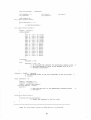
ABSTRACT
LIST OF FIGURES..............................................................................................................................................8
PREFACE............................................................................................................................................................... 9
1. INTRODUCTION.............................................................................................................................................9
2. BACKGROUND THEORY......................................................................................................................... 14
2.1 Introduction..................................................................................................................14
2.2 Subsumption Architecture......................................................................................... 15
2.2.1 Introduction.......................................................................................................... 15
2.2.2 Functional Decomposition.................................................................................. 15
2.2.3 Behavioural Decomposition...............................................................................16
2.2.4 Advantages/Disadvantages of Subsumption Architecture............................... 18
2.2.5 Application of Subsumption Architecture to the Project................................. 19
2.3 Computational Neuroethology...................................................................................20
2.3.1 What is Computational Neuroethology?........................................................... 20
2.3.2 Beer’s W ork.........................................................................................................21
2.3.3 Application of Computational Neuroethology to this Project.........................24
2.4 Simple Genetic Algorithms........................................................................................ 26
2.4.1 A definition of Simple Genetic Algorithms...................................................... 26
2.4.2 What’s new?......................................................................................................... 27
2.4.3 Genetic Fitness.....................................................................................................28
2.4.4 Genetic Operators............................................................................................... 29
2.4.5 Application of Simple Genetic Algorithms to this Project..............................31
2.5 Computational Embryology.........................................................................
2.5.1 Phenotype Growth....................
32
32
2.6 Conclusion...................................................................................................................34
3. HARDWARE IMPLEMENTATION DETAILS.................................................................................... 35
3.1 Introduction..................................................................................................................35
3.2 Hardware Environment Overview............................................................................ 36
3.3 Robot Single Board Computer (SBC) Details......................................................... 41
3.3.1 Introduction..........................................................................................................41
3.3.2 Aspirations........................................................................................................... 41
3
3.3.3 Operation of the SBC.........................................................................................43
3.3.4 Summary.............................................................................................................. 45
3.4 Robot/SBC Interface.........................................................................
47
3.4.1 Introduction..........................................................................................................47
3.4.2 Beginnings........................................................................................................... 47
3.4.3 Operation and Description..................................................................................48
3.4.4 Summary.............................................................................................................. 50
3.5 The Robot.............................................................................................................. .
51
3.5.1 Groundings........................................................................................................... 51
3.5.2 Description........................................................................................................... 51
3.5.3 Summary.............................................................................................................. 54
3.6 Behavioural Evaluation Environment....................................................................... 57
3.6.1 Introduction.......................................................................................................... 57
3.6.2 Description........................................................................................................... 57
3.7 Summary......................................................................................................................59
4.
SOFTWARE IMPLEMENTATION DETAILS....................................................................................60
4.1 Introduction..................................................................................................................60
4.2 Paragon Cross compiler............................................................................................. 63
4.2.1 Introduction..........................................................................................................63
4.2.2 O peration......................................................
63
4.2.3 Summary.............................................................................................................. 64
4.3 Simple Genetic Algorithm Software......................................................................... 66
4.3.1 Introduction and Reasoning............................................................................... 67
4.3.2 Application........................................................................................................... 69
4.3.3 Genetic Coding Breakdown................................................
71
4.3.4 Random Number Generation............................................................................. 72
4.3.5 SGA Operators.....................................................................................................74
4.3.5.1 The Genotype Selection Function...............................................................74
4.3.5.2 The Mutation Function................................................................................76
4.3.5.3 The Crossover Function.............................................................................. 78
4.3.5.4 Genetic Parameter Choices......................................................................... 81
4.3.6 Summary.............................................................................................................. 81
4
4.4 The Network Development Program.........................................................................83
4.4.1 Introduction.......................................................................................................... 83
4.4.2 Origin of the Idea................................................................................................. 84
4.4.3 How Does It Work? (The Rules)........................................................................ 85
4.4.3.1 General Rules................................................................................................85
4.4.3.2 Link Growth Dynamics................................................................................86
4.4.3.3 Node Division Dynamics.............................................................................86
4.4.4 Implementation of the Rules...............................................................................88
4.4.5 Network Download..............................................................................................89
4.4.6 The Genotype Parameter Decoding................................................................... 91
4.4.7 Network Growth.................................................................................................. 94
4.4.8 Summary.............................................................................................................. 95
4.5 Simulator and Simulation.......................................................................................... 97
4.5.1 Introduction.......................................................................................................... 97
4.5.2 Operation of the Neural Network....................................................................... 98
4.5.3 Simulator and Simulation Development..........................................................102
4.5.4 Simplifications...................................................................................................104
4.5.4.1 Simplification 1 (Internal Conductances)................................................ 104
4.5.4.2 Simplification 2 (Integers)......................................................................... 105
4.5.4.3 Simplification3 (Neural Node Structure)................................................ 107
4.5.4.4 Simplification 4 (Neural Node Update Routine)..................................... 110
4.5.4.5 Final Revision (Timing).............................................................................112
4.5.5 Node Types........................................................................................................ 113
4.5.5.1 Neural Node Description........................................................................... 113
4.5.5.2 Generator N odes........................................................................................ 115
4.5.5.3 Output N odes............................................................................
116
4.5.6 Summary............................................................................................................ 116
5. BEHAVIOURAL EVALUATION................................................................................................... 119
5.1 Introduction................................................................................................................119
5.2 What is good behaviour?......................................................................................... 121
5.3 The R ules...................................................................................................................123
5.4 Summary.................................................................................................................... 125
5
6. RESULTS..............................................................................................................................................126
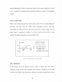
6.1 Introduction................................................................................................................126
6.2 Two Runs................................................................................................................... 128
6.2.1 Run 1................................................................................................................... 128
6.2.2 Run 2 ...................................................................................................................133
6.3 Results Conclusions..................................................................................................135
6.3.1 Simple Genetic Algorithm................................................................................135
6.3.2 Overall Framework............................................................................................135
7. CONCLUSION..................................................................................................................................... 137
7.1 Subsumption Architecture....................................................................................... 138
7.2 Computational Neuroethology................................................................................. 140
7.3 Computational Embryology & Genetic Algorithms.............................................. 142
7.4 Other Issues................................................................................................................145
7.5 Final Conclusions..................................................................................................... 147
8. BIBLIOGRAPHY................................................................................................................................ 149
APPENDIX A ..................................... PARAGON C CROSS COMPILER CONFIGURATION FILE
APPENDIX B ........................................................................ NEURAL NODE UPDATE EQUATIONS
APPENDIX C ...................................................................RANDOM NUMBER GENERATION SUITE
APPENDIX D ................................................... INTERFACE FROM MC68000 SBC PI/T TO ROBOT
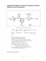
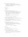
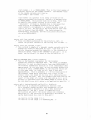
APPENDIX E .......................................................................... EXAMPLES OF NETWORKS GROWN
6
Abstract
An Experimental Design Framework for Evolutionary Robotics
Robert McCartney B.Eng. (Hons.)
Based on the failures of work in the area of machine intelligence in the past, a new
paradigm has been proposed: for a machine to develop intelligence it should be able to
interact with and survive within a hostile dynamic environment. It should therefore be
able to display adaptive behaviour and respond correctly to changes in its situation. This
means that before higher cognitive properties can be modeled, the modeling of the lower
levels o f intelligence would be achieved first. Only by building on this platform of
physical and mental abilities may it be possible to develop true intelligence. One train of
thought for implementing this is to control and design a robot by modeling the
neuroethology o f simpler animals such as insects.
This thesis outlines one approach to the design and development of such a robot,
controlled by a neural network, by combining the work of a number of researchers in the
areas of machine intelligence and artificial life. It involves Rodney Brooks’
subsumption architecture, Randall D. Beer’s work in the area of computational
neuroethology, Richard Dawkins’ work in the area of biomorphs and computational
embryology and finally the work of John Holland and David Goldberg in genetic
algorithms.
This thesis will demonstrate the method and reasoning behind the combination of the
work o f the above named researchers. It will also detail and analyse the results obtained
by their application.
7
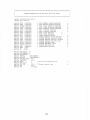
List of Figures
F ig u r e 2.1 F u n c t io n a l D e c o m p o s it io n D e s ig n S t r u c t u r e ..................................................................................16
F ig u r e 2 .2 B e h a v io u r a l l y B a s e d D e c o m p o s it io n D e s ig n S t r u c t u r e ...........................................................18
F ig u r e 2.3 N e u r a l N o d e s t r u c t u r e im p l e m e n t e d b y B e e r ................................................................................ 23
F ig u r e 2 .4 T e r m s u s e d in r e f e r e n c e t o S im p l e G e n e t ic A l g o r i t h m s ...........................
27
F i g u r e 2 .5 A s c h e m a t ic o f s im p l e c r o s s o v e r s h o w in g t h e a l ig n m e n t o f t w o s t r in g s a n d t h e
PARTIAL EXCHANGE OF INFORMATION, USING A CROSS SITE CHOSEN AT RANDOM....................................30
F ig u r e 3.1 G r a p h ic a l D e s c r ip t io n o f H a r d w a r e E n v ir o n m e n t ......................................................................37
F ig u r e 3 .2 R o b o t M o t o r O u t p u t C o d i n g ...................................................................................................................... 4 4
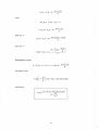
F ig u r e 3.3 S u m m in g A m p l if ie r C o n s t r u c t io n ............................................................................................................48
F ig u r e 3.3 T h e R o b o t ................................................................................................................................................................ 53
F ig u r e 3 .4 I m p r o v e d S e n s o r y f r a m e w o r k .................................................................................................................. 55
F ig u r e 3.5 B e h a v io u r E v a l u a t io n E n v i r o n m e n t ...............................................
58
F ig u r e 4.1 T e r m s u s e d in r e f e r e n c e t o S im p l e G e n e t ic A l g o r i t h m s ........................................................... 67
F ig u r e 4 .2 C o d in g o f G e n o t y p e s P r o d u c e d b y S im p l e G e n e t ic A l g o r i t h m .............................................71
F i g u r e 4.3 G e t _ O n e _ B e r n o u l l i ( ) ..........................................................................................
72
F ig u r e 4 .4 g e t _ O n e _ U n if o r m ( ) .......................................................................................................................................... 73
F ig u r e 4 .5 G e t _ M s r 8 8 ( ) .......................................................................................................................................................
73
F ig u r e 4 .6 S e t _ M s r 8 8 ( ) ...........................................................................................................................................................73
F ig u r e 4 .7 T h e S G A S e l e c t () F u n c t i o n ..........................................................................................................................75
F ig u r e 4 .8 I m p l e m e n t a t io n o f t h e S G A M u t a t io n o p e r a t o r ........................................................................... 77
F ig u r e 4 .9 F u n c t io n in C t o im p l e m e n t t h e c r o s s o v e r o p e r a t o r .................................................................. 80
F ig u r e 4 .1 0 G e n e t ic P a r a m e t e r s U s e d .......................................................................................................................... 81
F ig u r e 4 .1 1 I l l u s t r a t io n o f n o d e d iv is io n d y n a m ic s .............................................................................................88
F ig u r e 4 .1 2 C o d in g o f G e n o t y p e s P r o d u c e d b y S im p l e G e n e t ic A l g o r i t h m .......................................... 92
F ig u r e 4 .1 3 C o n t r o l l in g f u n c t io n f o r N e t w o r k G r o w t h .................................................................................94
F ig u r e 4 .1 4 T y p ic a l F e e d f o r w a r d N e t w o r k A r c h it e c t u r e ..............................................................................99
F ig u r e 4 .1 5 N o n -L in e a r N o d a l In p u t /O u t p u t G a in C h a r a c t e r is t ic ........................................................ 108
F ig u r e 4 .1 6 O l d a n d N e w S t r u c t u r e s C o m p a r is o n .............................................................................................110
F ig u r e 4 .1 7 E q u a t io n u s e d t o u p d a t e n o d e in p u t v a l u e . (V c in f ig u r e 3 .3 ( b ) ) .................................. 111
F ig u r e 4 .1 8 N e u r a l N o d e s t r u c t u r e im p l e m e n t e d b y B e e r ..................................... ...................................... 115
F i g u r e 4 .1 9 N e u r a l N o d e M o d e l U s e d in P r o j e c t ...............................................................................................1 15
F ig u r e 4 .2 0 G a in c h a r a c t e r is t ic f o r O u t p u t N o d e s ........................................................................................ 116
F ig u r e 5.1 B a s ic B e h a v io u r a l S c o r i n g .......................................................................................................................124
F ig u r e 5 .2 S e n s o r A c t iv a t io n S c o r i n g ........................................................................................................................124
F ig u r e 6.1 O p e r a t io n o f S G A f o r R u n 1.............................
130
F ig u r e 6 .2 A n t i -C l o c k w is e A r c M o v e m e n t E x h ib it e d b y R o b o t ..................................................................132
F ig u r e 6.3 O p e r a t io n o f S G A f o r R u n 2 .......................................................................................................................134
F ig u r e B 1 N e u r a l N o d e u s e d in S im u l a t o r a n d S i m u l a t io n ................................................................................ i
F ig u r e B 2 N e u r a l N o d e u s e d B Y B E E R
.......
8
m
Preface
This thesis represents the combination and completion of a number of works. It was
completed with the School of Electronic Engineering while registered as a student of the
Integrated B.Eng./M.Eng. study programme. For that reason a number of other
documents relating to this project have previously been produced [23,24,25,26]. The
integrated programme allows students to initiate research for the award of a Masters
degree in Engineering while registered as an undergraduate.
9
1. Introduction
This thesis is about machine intelligence. It has been inspired by the lack of success in
recent years in the areas of connectionism, neural networks and expert systems. All of
these areas have promised much but unfortunately delivered very little. None of these
areas have made significant progress in developing systems which display an
intelligence that is not either defined within strict operational boundaries or uses
simplistic, representationalised input data. Recently however, a number of researchers
have attempted to approach the problem of modeling machine intelligence from a new
direction. The new direction which they propose is very simple and is the foundation
stone upon which this thesis is based. They propose that, in order for a machine to
exhibit higher level cognitive properties, it is first essential that the machine be able to
deal with the real environment in which it exists.
The evolution of human intelligence is worth considering at this point as this is the
intelligence that is referred to when people discuss the creation of artificial intelligence.
The planet Earth is approximately 4.6 billion years old, and single cell life first appeared
on it about 3.5 billion years ago The first photo synthetic plants appeared about 1 billion
years later. Two billion years after that, the first vertebrate animals and fish appeared
and then about 450 million years ago insects appeared. Reptiles were around about 370
million years ago and mammals arrived only about 250 million years ago. The human
race appeared approximately 2.5 million years ago; descended from the first apes who
appeared only 16 million years before that. Human level intelligence only first became
10
apparent with the discovery of agriculture some 19,000 years ago, writing about 5,000
years ago and “expert” knowledge only in the last few centuries. This means that
evolution has spent only 0.005% of 3.5 billion years of the evolutionary time span
dealing with higher level intelligence. This could be seen to suggest that the capabilities
of problem solving, language, reason and expert knowledge are either made more
simple as a result of, or alternatively dependant on, the ability of a being to deal
interactively with the hostile dynamic environment in which it finds itself.
In continuation with this theme, a machine intelligence should not be designed within a
cotton wool model of the real world and then be expected to be capable of dealing with
the real world at some later stage. The only valid model for the real world in all its
chaotic glory is the real world itself. The functional and reality gap between simulation
of intelligent behaviour and the implementation of intelligent behaviour is too great. In
everyday operation an intelligent machine should be able to adapt to changes in its
situation and environment. It is important that it be able to protect itself from physical
damage (for example stop itself driving off a cliff if a bridge that existed the day before
was now no longer present). The machine must be able to differentiate between, and
deal with, different classes of problems and come to an optimum, scenario dependant
solution, rather than simply follow an algorithmic path to a pre-defined answer in a pre
defined situation.
Therefore, it is essential that the machine be multi-tasking and fully aware of the world.
For example, even taking a parcel from a position x to another position y requires a vast
11
amount of physical and mental capabilities. The controlling intelligence must be
continually prioritising problems and coming to optimum solutions to complete the task.
To illustrate, consider some of the tasks which must be completed. Detect and grasp the
parcel, plan route from x to y based on internal (or external) area map, monitor terrain to
avoid becoming stuck or damaged, continually choose optimum path around obstacles,
monitor progress, monitor position and physical condition, etc. all while remembering
its primary goal of delivering the parcel.
The next question is, of course, how do we design a robot that can behave like this? Due
to the incredible complexity of the human brain it is currently impossible to model it
properly. So a number of researchers have proposed that to design or to create a
machine intelligence comparable with human intelligence it is first essential to model
the simpler intelligence of simple animals such as insects. Using this modeling and
neurobiological knowledge it should then be theoretically simpler to work upwards from
there. This thesis defines and evaluates a single approach to the development of a
framework for the development of a low level adaptive machine intelligence which
could be continually updated and augmented. The framework is designed to create a
machine that may be continually improved using new found knowledge in the areas of
biology, robotics, artificial intelligence and natural systems modeling.
This thesis is divided into a number of different sections. These are:
1. Thesis Overview.
2. Background theory and description of:
•
Subsumption Architecture.
12
•
Genetic Algorithms.
•
Computational Embryology.
•
Computational Neuroethology.
3. Details of:
•
Adaptation of background theory to application.
•
Hardware descriptions of robot, controlling microprocessor board and
interface.
•
Software written for application.
4. Results and analysis.
•
Description.
•
Evaluation.
•
Recommendations
5. Conclusion.
13
t
2. Background Theory
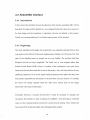
2.1 Introduction
In this section, the theories, ideas and inspirations behind the project will be outlined.
More detailed knowledge of these topics can be obtained from the references given, as it
is not feasible to provide more precise details and/or examples within the confines of
this thesis.
The work of Rodney Brooks[3,4,5] whose subsumption architecture idea is one of the
cornerstones of the masters degree project, is outlined in section 2.2. The work of
Randall D. Beer[2] who has designed and simulated the operation of neural networks
based on a computational neuroethological approach, along with the modifications that
were necessary for its application to this project are detailed in section 2.3. Finally,
based on the work of Goldberg[14] and Dawkins[9,10,ll], genetic algorithms and their
application to this project is presented in sections 2.4 and 2.5.
The information in these sections is not sufficient to understand the complexities of the
fields; rather it serves only as a brief introduction to their basic concepts. This is to
make the theoretical basis o f the project more tangible: to bring together, and show the
relationship between, all the different aspects of the project work being done
14
2.2 Subsumption Architecture
2 .2 .1 I n tr o d u c tio n
As stated above, one of the main sources of inspiration for the Master’s project and
which underlies the work done is the work of Rodney Brooks[3,4,5]. Brooks’ idea is
that existing approaches to the development of machine intelligence are fundamentally
flawed. He proposes that in order for a machine to develop intelligence it is first
essential that the machine be able to deal successfully with a hostile external
environment. To this end he has proposed a new design structure for intelligent
machines which is based on a behavioural design methodology rather than the more
accepted functional design decomposition currently used by many researchers in the
areas of artificial intelligence and Robotics. In this section the two approaches to the
design of controlling frameworks will be compared and the advantages of the
subsumption architecture approach described.
2 .2 .2 F u n c tio n a l D e c o m p o s itio n
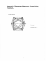
Figure 2.1 represents a functional decomposed design structure for generating
‘intelligent’ behaviour in machines. The robot control algorithm designed using this
approach would incorporate as many solutions as were necessary/possible to enable the
robot to interact with its environment and thus exhibit some form of intelligent
behaviour. However, due to the serial nature of this structure as well as the complex
interactions and message passing techniques employed by this form of design, it fails.
This failure is illustrated by the fact that if any particular section of the robot were to fail
or become so obsolete as to be rendered useless then an entirely new robot would have
to be designed and built to overcome the failure or to upgrade the hardware. This is at
the expense of money, materials and time. Obviously from a robustness, as well as a
practical viewpoint, this method of design is unacceptable in the long run.
Figure 2.1 Functional Decomposition Design Structure
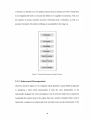
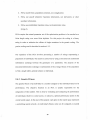
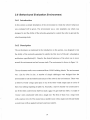
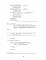
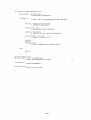
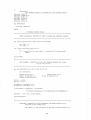
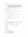
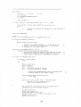
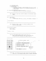
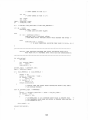
2 .2 .3 B e h a v io u r a l D e c o m p o sitio n
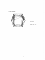
However, shown in figure 2.2 is a diagram which describes a much different approach
to designing a robot which demonstrates at least the same functionality as the
functionally designed one. From the diagram it can be seen that rather than a single link
connecting the sensory input to the output, there are a number of parallel links. Each of
these links is graded on a behavioural level and each level uses the functionality of the
16
previous levels to carry out its own tasks. To illustrate; the construction of such a robot
begins with the design of a very simple robot which successfully implements its own
low-level behavioural tasks such as the avoidance of objects. When this level of
behaviour has been successfully implemented, tested and proven within a real
environment, the next level of behaviour is designed. This level could be, for example, a
wandering behaviour. To enable the robot to apparently wander around its environment
a level of control is added which takes advantage of the lower level’s behavioural
capabilities. It subsumes control of the lower level. This robot is then tested fully and
when it has been found to wander successfully, the next level of behavioural control
(perhaps an environmental mapping behaviour) is designed, added and tested. The
addition of each of the completed stages offers a higher level of overall complexity and
intelligent behaviour to the robot.
Each level of the architecture operates independently of the others but each level can
subsume control o f the levels lower than itself in the behavioural hierarchy and use them
to its own advantage. This process, Brooks believes, will eventually lead to a machine
which can make its own decisions on abstract, logical and pure reflex levels and thus
potentially demonstrate an intelligence far outstripping anything currently implemented
by functionally designed robots.
17
SENSORS
i
fi
Avoid
Objects
ji
1
Wander
Explore
2
3
I
Monitor
Changes
5
Build
Maps
4
I
Identify
Objects
I
I
Plan
changes to
the w orlds
I
Reason about
the behaviour
o f objects g
I
I
Increasing Level
of Intelligent Behaviour
ACTUATORS
Figure 2.1 Behaviourally Based Decomposition Design Structure.
2 .2 .4 A d v a n ta g e s /D is a d v a n ta g e s o f S u b s u m p tio n A r c h ite c tu r e
The beauty of the subsumption architecture is that, due to the modular nature of both the
robots intelligence and construction, should any particular level be found to be faulty or
technologically redundant, then only the offending section need be redesigned - not the
entire robot. This saves on money, materials and time. One substantial drawback
however is that a great deal of parallel computational power is potentially necessary to
implement such a structure. As a result, the robot could (in today’s world) be quite
expensive to implement initially. However, due to the ease of maintenance and upgrade
involved with a truly subsumptive robot design, the architecture prevents (as much as
possible) the robot becoming obsolete due to the failure or redundancy of a single
section.
18
2 .2 .5 A p p lic a tio n o f S u b su m p tio n A r c h ite c tu r e to th e P ro ject
Taken in the form as described by Brook, subsumption architecture is a long term
design configuration. Brooks used Finite State Machines to implement each behavioural
level in the architecture. However, as is discussed in more detail in the next section, this
is obviously not a very biologically inspired approach to the implementation of the
subsumption architecture ideal. Subsumption architecture is used simply as a ‘container’
for all the other facets of the project. It is the primary cornerstone of the project but in
itself is not implemented fully. To be implemented fully, a second level of behaviour
would have to be successfully implemented above a successful first level. Within the
context of the project only the first behavioural level was implemented and explored.
Therefore, any further reference to subsumption architecture must be seen in that
context.
19
2.3 Computational Neuroethology
Brooks’ subsumption architecture control structure is based on the interaction of many
Finite State Machines(FSMs)[4], This offers an ease of implementation because the
design of FSMs is not excessively complex if the problem is well defined. However (as
was discussed in the introduction), in the context of this project it was decided to use a
more biologically inspired choice of control structure for each level of behaviour.
Following research in the area of neural networks, it was decided that they could offer
what was required. The type of neural network control structure chosen to implement
was a heterogeneous neural network structure. The design and construction of this form
of neural network was first encountered in the work of Randall Beer [2]. In this work he
describes the use of a technique known as computational neuroethology.
2.3.1 W h at is C om putational N euroethology?
Beer describes computational neuroethology as:
“...T h e d ir e c t u se o f b e h a v io u r a l a n d n e u r o b io lo g ic a l id ea s f r o m
s im p le r n a tu r a l a n im a ls to c o n s tr u c t a r tific ia l n e r v o u s s y s te m s f o r
c o n tr o llin g th e b e h a v io u r o f a u to n o m o u s a g e n ts ”
[2][p xvi].
D. T. Cliff in his paper[8] also delivers a concise and studied discussion on
computational neuroethology. His conclusion references the ability of networks
designed
using
computational
neuroethology
20
to
span
the
MacGregor-Lewis
stratification1 [26]. He references material common to the area of this thesis. Principally,
he references extensively the work of Rodney Brooks. In this paper he provisionally
defines computational neuroethology as the
“...s tu d y
o f n e u r o e th o lo g y
u s in g
th e
te c h n iq u e s
o f c o m p u ta tio n a l
n e u r o s c ie n c e ”.
[8]
In particular he notes that a very specific aspect of computational neuroethology is the
“...in c r e a s e d a tte n tio n to the e n v ir o n m e n t th a t the n e u r a l e n tity is a
com ponent o f ”
[8 ]
2.3.2 B e er ’s W ork
In the previous section 2.2 on subsumption architecture, reference was made to Brooks’
belief that work in the area of artificial intelligence was fundamentally flawed in its
approach[3,4,5]. Beer, in his work, makes a very similar statement in the preface of his
book[2], saying that thinking in this area
“...h a s b e e n d o m in a te d b y th e n o tio n th a t in te llig e n c e c o n s is ts o f the
p r o p e r m a n ip u la tio n o f s y m b o lic r e p r e se n ta tio n s o f the w orld. ”
[2]
1 A sim ple taxonom y o f levels o f analysis. C liff however, makes reference to the stratification as being potentially
non-ideal and perhaps requiring a further detailing o f levels[8].
21
Certainly this seems to tie in very well on a conceptual level with Brooks’ thesis of
using the world as its own model[4], It was viewed at the beginning of this project that a
marriage of the work’s o f these two men would be both interesting as well as being,
potentially, a rewarding approach. This reward being based on the combination of the
real time efforts of Brooks[3,4,5] and the perceived mental processing offered by Beer’s
neural network structure [2], Beer himself states that simpler animals possess a degree of
adaptive behaviour that far exceeds that available to the most complex of artificial ones
[2]. This level of processing power seemed ideal for a real time robotic implementation.
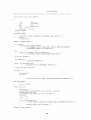
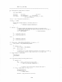
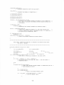
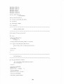
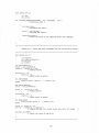
Beer successfully implemented and documented [2] a simulated insect. Its behaviour
was due to a neural network which was based on a map of the understood neural
mechanics of the insect Periplaneta Americana: the American cockroach. The simulated
insect, using a neural network constructed using neural node models of the type
described in figure 2.3 below, successfully traversed its simulated environment. It
achieved some of its specified goals, such as food-finding, and it emulated the
behaviour of many real insects by, for example, performing an edge following
behavioural pattern around its environment.
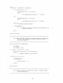
Beer attributes this success to, among other things, the closeness of the neural model he
employed to the structure of real neurons[2]. He refers to the work of Llinas[22] and
emphasises the findings of Selverston[32], Specifically he emphasises the fact that nerve
cells contain a wide variety of active conductances which appear to allow them to
demonstrate complex time-dependant behavioural responses to stimulation. They can
also allow demonstrate apparently spontaneous activity when the network is active.
22
Selverston studied the interactions of active conductances at a cellular level and found
that they appeared to be crucial to the function of neural circuits[32].
Firing
Frequency
Membrane
Properties
Figure 2.2 Neural Node structure implemented by Beer
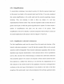
Unfortunately, Beer’s simulation ran as much as ten times slower than real
time[2][p.63]. This meant that any attempt to directly recreate the same networks and
behavioural patterns in real time would be unattainable using the existing hardware
resources. This posed a large problem but the solution chosen was to simplify the neural
node model. Hence, reducing the computational processing power required and thus
allowing small networks to operate and be successfully updated in real time. This was
necessary to achieve the first goal of the project which was to have a real time robot
behaving in accordance with the initial behavioural levels of Brooks’ subsumption
architecture [4],
23
2 .3 .3
A p p lic a tio n o f C o m p u ta tio n a l N eu r o e th o lo g y to th is P r o ject
The application o f the computational neuroethology paradigm to this project was to
model the construction of the nervous system of a simple animal such as an insect. It
was decided to make the implementation as facile as possible by incorporating wheels
into the robot structure rather than using mechanical legs. This, it was viewed, would
allow the overall framework to concentrate on the sensory response characteristics of
the robot. The generation of a mechanical gait controller was viewed as superfluous at
this early stage of research.
The goal of this modeling was the production of a neural network which would control a
robot in real time. The network, designed on a computational neuroethological basis,
would be heterogeneous in nature. This meant that it would not be a physically fixed
structure neural network form (as compared to a multi-layer perceptron network[31] for
example). Also the individual neural nodes within this type of neural network have
more than a single parameter governing their input/output behaviour. As Beer
successfully demonstrated[2], this extra variability can mean that this form of network
should potentially be able to display more complex functionality than a fixed structure,
single variable neural network. This variability also allowed the use of fewer nodes and
hence computation. This is very useful in an application concerned with real time
operation and control such as robotics. Unfortunately it also means that none of the
standard learning algorithms associated with existing neural network models are
applicable. Hence each network must be designed manually.
24
This application o f this type of neural network structure as a robot controller, as well as
the real time advantages, seems to tie in very well, on an inspirational level, with
Brooks idea of a subsumption architecture for the implementation of machine
intelligence. However, the networks designed by Beer (which are based on existing
neurobiological maps of small insects) only operated in the very strictly controlled
conditions of a simulated environment within a computer simulation[2]. When this
project was originally started, this computational neuroethological methodology for
neural network design had not been used to successfully develop a real time robot
controller dealing with a real environment. However, Beer does mention this particular
application in the conclusion of his book[2].
As stated above, one of the main problems involved with using the work of Beer as it
stood was that the simulation which implemented his neural networks for the control of
his simulated insect operated very slowly. The simulation ran at a speed equivalent to
three to ten times slower than real time[2][p.63]. For the purposes of this project the
neural node model which Beer used had to be simplified (accepting the resultant
degradation in an individual neural node’s functional potential). This was in order to
speed up the operation of the networks and allow real time operation. This is obviously
essential in a real environment. This simplification was made doubly necessary as the
networks produced in this project were to be run on a Motorola ‘Force’ board. This
board used a MC68000 processor with a bus speed of only 8 MHz. The details of the
simplification eventually used for the neural node are given in section 4.5.4.3.
25
2.4 Simple Genetic Algorithms
2 .4 .1 A d e fin itio n o f S im p le G e n e tic A lg o r ith m s
The third academic source for the thesis is the work of David E. Goldberg [14],
Goldberg's work is in the area of Genetic Algorithms. Genetic Algorithms (GAs) can be
used for finding a solution to problems in non-linear or complex problem spaces. GAs
differ greatly from the traditional algorithms used for problem solving. GAs use a
number of rules to ‘find’ an optimum solution to a given problem rather than derive a
precise solution to a precise problem. They draw their inspiration from the apparent
ability of the DNA structures contained in all living matter to solve problems in a
gradual and optimum seeking manner.
The operation of genetic algorithms revolves around the use of parameters coded in
string form, (which in the case of this project is in binary format). This string form is
referred to as the genetic coding. GAs, in their simplest form, use constructive and
destructive mutations of the genetic coding, a structured yet randomized information
exchange between strings and a guiding ‘objective’ function in their search for a
solution. The objective function guides the algorithm towards an optimal solution (and
hopefully the optimum) in a given problem space. The optimal solution is evolved
gradually as the algorithm 'traverses' the problem space. The location of the optimal
solutions in a search is dependant on a number of parameters. These parameters include
the availability of a smooth genetic search space, the correct setting of the genetic
string’s internal parameters (see section 4.3.3) and a well defined objective function.
26
Simple Genetic Algorithms (SGAs) are, as the name suggests, the most basic
implementation of genetic algorithms. The term Simple Genetic Algorithm is used
throughout this text because the code used to implement the genetic algorithm operation
is based on the PASCAL code given in Goldberg's book [14][chpt.l], This PASCAL
code is called a simple genetic algorithm by Goldberg and the continued use of this term
is purely for the sake of remaining consistent with the material in the reference text.
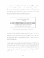
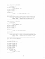
To prevent confusion the main terms and abbreviations used in this section and the
remainder of the thesis in reference to simple genetic algorithms are now explained:
SGA
Simple Genetic Algorithm
Search Space
The problem space of the simple genetic algorithm.
Genotype
Bit string which encapsulates the parameter set of an individual.
Phenotype
Entity created from the decoding of a Genotype.
Individual
Refers to the Genotype and Phenotype as a single unit.
Fitness
Value assigned to individuals based on their performance used
in reproduction of individuals.
Population
A collection of individuals.
Generation
A particular instance of a Population.
Figure 2.4 Terms used in reference to Simple Genetic Algorithms
2 .4 .2 W h a t ’s n e w ?
So what are the fundamental differences between SGAs and more traditional
algorithms? Goldberg specifies four ways in which SGAs differ from traditional
optimisation techniques.
1. SGAs work with a coding of the parameter set, not the parameters themselves.
27
2. SGAs search from a population of points, not a single point.
3. SGAs use payoff (objective function) information, not derivatives or other
auxiliary information.
4. SGAs use probabilistic transition rules, not deterministic rules.
[14][p.7],
SGAs require the natural parameter set of the optimisation problem to be encoded as a
finite length string over some finite alphabet. For this project the coding is a binary
string in order to minimise the effects of single mutations in the genetic coding. The
precise coding used is described in section 4.3.3.
The operation of the SGA involves processing a number of strings representing a
population of individuals. The search is carried out by using a structured yet randomised
information exchange between the genotypes of a population. The purpose of the
structured information exchange is optimisation of the average fitness of the population
to find a single stable, optimal solution or individual.
2 .4 .3 G e n e tic F itn e s s
The genetic fitness of an individual is a number assigned to the individual based on its
performance. The objective function in an SGA is usually responsible for the
assignation of this number. This is done by evaluating and comparing the performance
of individuals relative to some known, or unknown, optimal performance points in the
overall search space. In the case of this project: each point in the search space represents
a controlling neural network. An individual's fitness value can be compared, in natural
28
selection terms, with the ability of an individual to survive and mate with another
individual. The objective function is usually a function within the scope of the SGA
program itself. However, for this project, due to the difficulty in defining what
constitutes ‘good’ behaviour (see section 5.2), it falls upon a human tester to evaluate
the performance and determine the fitness of the individuals.
2 .4 .4 G e n e tic O p e r a to r s
This information exchange between individuals is implemented using a number of
functions, the individuals' fitness values and what are referred to as genetic operators. In
SGAs (as applied in this project) these are a reproduction operator, a crossover (or
mating) operator and a mutation operator. The genetic operators are the basis of the
operation of an SGA.
The reproduction operator is a process in which genotypes are copied according to the
fitness of their respective individual's values. The higher the fitness of an individual,
relative to the fitness of other individuals in the same generation, then the higher the
probability o f that individual contributing one or more offspring to the next generation.
The mutation operator is used to prevent the complete loss of important information.
This can happen when the algorithm begins to converge towards an optimum. It is a
probabilistic process which switches the value of a single bit location in a genotype,
from a 1 to a 0 or vice versa for example. It allows the algorithm the possibility of
29
2
retrieving an important bit configuration (or schema) which may have been lost
between generations.
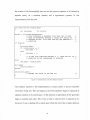
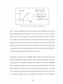
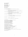
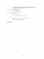
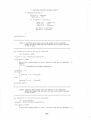
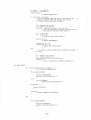
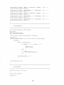
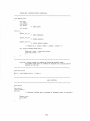
Finally, the operation of the crossover operator is shown in figure 2.5 below. It is a
process whereby the genotypes of two individuals, chosen by the reproduction operator,
are mated and exchange information. The crossing site is chosen at random and can be
at any point along the aligned strings. This means that simple reproduction without
information exchange is possible (i.e. the cross site can be chosen at the end or the start
of strings).
After Crossover
Before Crossover
Crossing Site
String 1
1111 1111
11110000
New String 1
00001111
New string 2
Crossover >
/
String 2
0000 D000
Figure 2.3 A schematic o f simple crossover showing the alignment o f two strings and the partial exchange o f
information, using a cross site chosen at random.
It is important to note that the SGA may not find a perfect solution to a given problem
(it may not exist!). It strives only to improve on existing proposed solutions using the
genetic operators described.
2 A schem a is a sim ilarity tem plate describing a subset o f o f strings w ith similarities at certain string positions. For a
m ore com plete description refer to G oldberg [14] or Holland [20],
30
2 .4 .5 A p p lica tio n o f S im p le G en etic A lg o rith m s to th is P r o ject
The simple genetic algorithm is the most basic form of the genetic algorithm available.
There are many others documented even within the texts already referred to [14,19].
However, I think that it is pertinent to re-emphasise that this thesis offers only a primary
investigation into the area of the combined use of many different works and areas of
expertise. That is why the majority of modifications made to existing works were
simplifications (e.g. use o f the SGA, the neural model used, the parameterisation of the
neural model (see chapter 4)). The simplifications were used in order to attempt to
obtain fundamental results which would verify the potential success based on the
combination of the underlying processes.
For the purposes of this project; reproduction, crossover and mutation are the three
genetic operators used. As stated above, the fitness of an individual network is evaluated
by the network designer and not by an objective function within the program. Also the
reproduction function does not allow generations to overlap. This was a decision made
to simplify the implementation of the SGA.
Now that the structure for the algorithm's operation has been described, how does the
genotype become a phenotype? This is achieved by the application of computational
embryology.
31
2.5 Computational Embryology
2 .5 .1 P h e n o ty p e G r o w th .
Goldberg's work is being used in conjunction with the work of Richard
Dawkins[9,10,11] to create neural networks for robotic control. In his work Dawkins
uses genetic algorithms and a 'development' routine (which decodes the genotypes) to
produce pictures on a computer screen that could be considered biological in form. He
calls these pictures biomorphs and some do indeed resemble (in a two-dimensional
sense) insects, some resemble trees and they can be made to produce a variety of
‘biological’ forms.
The pictures are generated using a development routine that decodes and uses the set of
parameters encapsulated in the genotypes. These are parameters like: the number of
times the recursive growth routine is called; the angle that branches or divisions in the
pictures take, the length of the branches, etc. The choice of which individual is the 'best'
or the most fit in a genetic algorithm sense is a purely arbitrary decision made by the
user. In Dawkins’ case this meant the reward of individuals who produced pictures that
resembled something biological in nature.
For the purposes of this project the growth idea is adapted and used to grow the neural
networks to control the robot. One difference lies in the fact that Dawkins does not use
crossover in his application of the genetic algorithm. The crossover operator is used in
the course of this project. It was hoped that by using the crossover operator that the
SGA could come to an optimum more quickly than by depending on mutation alone.
32
The networks are grown from a decoding of growth parameters encoded in the
genotype. The details of the genotype encoding and decoding are given in section 4.3.3.
33
2.6 Conclusion
In chapter 2 a general introduction to each of the main sections of the applied
background theory was given. The concepts of subsumption architecture, computational
neuroethology, computational embryology and genetic algorithms were introduced and
some details of their application to this project were given. The specifics of their
individual contributions to the project are detailed later in the thesis.
34
3. Hardware Implementation Details
3.1 Introduction
In this chapter, each o f the relevant hardware components of the design framework will
be described. The performance of each of the components will also be analysed and
suggestions for improvements detailed where appropriate. The sections that will be
described are the robot Single Board Computer (SBC) (section 3.3), the robot to SBC
interface (section 3.4), the robot itself (section 3.5) and finally the simulation
environment that the robot’s behaviour was observed in (section 3.6). Firstly however, a
general introduction to the physical hardware setup and connectivity will be presented in
order to allow the reader to see where each part of the hardware is in respect to all the
others. Overall, the hardware chosen for the implementation performed to varying
degrees of success. The problems, successes and recommendations for improvements in
the setup will be given at appropriate points within this chapter.
35
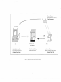
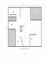
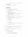
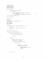
3.2 Hardware Environment Overview
In this section the overall hardware environment will be described in order to allow the
reader to appreciate the positions of all the constituent hardware sections of the
framework relative to each other. The hardware consists of a number of very distinct
parts, each of which is responsible for a number of different areas of the overall
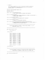
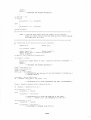
operation. A pictorial description of the environment is shown in figure 3.1.
As can be seen from the text in the picture, a large quantity of processing for the overall
framework is done on the PC. The PC is responsible for both the implementation of the
simple genetic algorithm and for the implementation of the artificial neural network
development routines. The PC also controls the generation of the network simulation
executable code which is transmitted to the SBC in MC68000 microprocessor assembly
code.
The format of the assembly code transfer is S I9 format[30]. The transferable code is
generated using the PARAGON C Cross Compiler[2 8] software which generates the
MC68000 assembly code from the source code written in the C programming language.
The human user also uses the PC for controlling the input of behavioural scores. Each of
the above software operations are detailed in chapter 4. The type of PC used varied over
the course of the project from an 80386SX
processor
36
personal
computer
to
a
Pentium
Human Observer
Network Behaviour Evaluation,
Fitness Score Input.
\} - Ò
MC68000 SBC
& Interface
Simple Genetic Algorithm,
Neural Network Development,
& Behaviour Score Logger.
Neural Network Simulator
& Robot D/A Interface.
Figure 3 .1 Graphical Description o f Hardware Environment
37
Neural Network Host.
(Operating in Behavioural Evaluation
Area. See Figure 3.6)
personal computer. The 386 was more than adequate for implementation of the overall
framework.
However, the increase in power was the direct result of the combination of a desire for
greater support for ancillary operations in the project (such as word-processing), and the
desire to decrease the software compilation times during development. Also, the
improved PC performance increased the general operation speed during neural network
evaluation runs. The evaluation of each network took approximately 4 minutes from
beginning to end and any increase in speed was a great advantage in simply preventing
boredom as each generation of robotic behaviour was evaluated. This was actually quite
an important issue as maintaining concentration was very important in evaluating the
performance o f the robot objectively.
The SBC is responsible for executing the software which implements the neural
network controlling the robot. Its sole responsibility is to run the software which reads
the robots sensory input and controls the corresponding motor output. The SBC uses an
MC68000 microprocessor.
Two different SBCs were used over the course of the project. The first was a
MOTOROLA MC68000 Educational Computer Board (ECB). However, the use of the
ECB was not satisfactory as it suffered significant hardware failure twice. The second
time this happened was at a crucial point in the project and the failure forced the project
to be delayed by about 6 weeks. In total, because of the attempt to continue to use this
board by waiting for replacement parts, over two months delay occurred before testing
38
and evaluation of the overall framework could be carried out. This only became possible
when it became obvious that it would be impossible to delay the project any further.
Eventually, a different SBC was selected, allowing work to continue. This new board
was also MC68000 microprocessor controlled but it had the added, and significant,
advantages of having both an 8 MHz microprocessor and a more reliable power source.
The previous SBC had only a 4 MHz microprocessor and significant problems with its
power source. These difficulties and their solutions are detailed in section 3.3 which
also discusses other issues pertinent to the SBC.
The next piece of hardware is the interface between the SBC and the robot. It acts as a
digital to analog converter for the robot motor output signals generated by neural
network software running on the SBC. It uses two power amplifiers to boost the power
of this converted output in order to drive the motors. It also passes the sensory
information, generated by the robot, to the SBC. The interface went through a number
of significant changes throughout the project. These changes are detailed in section 3.4
along with details of the final design of the board.
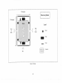
The final piece of hardware is the robot itself. The robot was constructed from Technic
LEGO® building blocks. It was ‘inherited’ from a previous project in the School of
Electronic Engineering and was redesigned and enhanced. A number of problems still
remain with the robot's construction and recommendations for its future enhancement
are detailed in section 3.5.3 along with the design as it stood at the end of the project.
The robot operates in a closed physical environment which is described in section 3.6.
39
Overseeing the operation of all this and responsible for the evaluation of the robot’s
behaviour in the real world is a human observer. The observer is responsible for
synchronising the overall evaluation process and inputs the scores assigned to the
robot’s behaviour into the PC. The details of this evaluation are given in chapter 5 .
40
3.3 Robot Single Board Computer (SBC) Details
3 .3 .1 I n tr o d u c tio n
In this section the robot SBC which was responsible for the implementation of the
neural network simulator software (see section 4.5) will be detailed. The responsibilities
of the SBC will be detailed and a description of the changes undergone in its physical
configuration over the course o f the project will be given. Also, the manner in which the
SBC communicated with the robot interface (see section 3.4.3) and the PC will be
described (see section 3.4.3). The difficulties encountered with the SBC, mentioned in
section 3.1, over the course of the implementation will be described. The reasoning
behind the choice of hardware will be given and recommendations for future
enhancements will be explored.
3 .3 .2 A s p ir a tio n s
The neural networks designed on the PC were each to be tested on the robot. When this
was decided, early in the project, the question of what the networks would be run on
was broached. A long term decision was made concerning this which on reflection may
seem a little optimistic in its aspirations. It was decided to execute the neural network
simulator software on a dedicated SBC rather than from the PC itself. The decision to
use a dedicated control board was made because it was hoped that, eventually, the robot
would become a single unit incorporating physical structure, power source and
microprocessor control board. It was hoped that this may even have been possible
within the time frame of this project. However, a significant degree of disruption
41
occurred which slowed the progress of the project. These difficulties will now be
detailed.
The original SBC used was a Motorola MC68000 Educational Computer Board (ECB)
[30]. The ECB had been used for a number of years within the School of Electronic
Engineering and was apparently quite old. It did not use a dedicated power supply and
was powered instead using a MINILAB power unit from the School of Electronic
Engineering laboratories and the first problem that occurred was in this power supply
setup. The power supply problem manifested itself by causing the SBC to periodically
reset itself. This caused more frustration than damage as all that was required was to
download the network simulator software to the SBC again. However, as every aspect
of the framework testing was quite time-intensive any delay was extremely discouraging
and disrupting.
The second, and more major problem that occurred was discovered to be due to, after
post failure analysis, to the physical condition of the original board used. Although the
ECB may have sufficed for a shorter term project it seemed unable to satisfy the
operational requirements it was under. Subsequently the ECB suffered two hardware
failures. These failures may not necessarily have been due directly to the power source
problems mentioned above (no detailed examination was carried out after the failures)
but they may have been related. No detailed examination was carried out because the
SBC being used was simply a tool for the project. It was perceived that it would have
been detrimental to the progress of the overall project to spend excessive time
examining the hardware failures.
42
The second of the hardware failures occurred at a point where all the constituent parts of
the framework were in a position to be tested together. The delay caused by this failure
was in excess of six weeks during which time all work effectively ceased as no testing
could be carried out on the work already done. The board was sent away to be repaired
but unfortunately the repair was not economical. Therefore, the ECB was replaced with
a different SBC.
This new SBC was much more successful and also stable. This may have been as a
result of the fact that it had a dedicated power supply. The new board was also obtained
from within the School of Electronic Engineering and was a Motorola FORCE Board.
As well as this dedicated and stable power source, the FORCE board also had an 8 MHz
processor speed which was an added advantage as the ECB only had a 4 MHz processor
speed. Any speed that could be gleaned at all from the setup was viewed, correctly I
feel, as an advantage to the real time aspect of the framework and its testing.
3 .3 .3 O p e r a tio n o f th e S B C
As mentioned previously, the SBC was responsible for the execution of the neural
network simulator software. This neural network software was downloaded in assembly
language format to the SBC, each time the SBC was turned on, in order to execute it.
This was necessary as the SBC could not store any user information after powerdown.
The software was transmitted from the PC using the KERMIT software transport
protocol[30]. The download situation was not as complicated as it may have been
because the SBC had a resident control system in its ROM which facilitated the
43
relatively pain-free receipt of software transmitted from an external source. The
software on the SBC could also be executed from the remote source. This facilitated the
implementation of a batch routine on the PC which automated the transmission of the
neural network simulator software as well as the neural networks produced by the
design framework.
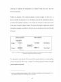
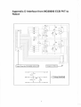
On the other side of the operation, the SBC communicated with the robot interface using
a Parallel Interface/Timer (PI/T) chip that was resident on the SBC. This chip transmits
the motor outputs in a digital format to the interface board. This format is an eight bit
binary number where the most significant 4 bits and the least significant 4 bits
corresponded to each of the motors. The motors are bi-directional, to allow the robot the
ability to reverse. The code relating the speed and direction of each of the motors is as
described in figure 3.2 below.
Binary Code
0000
Motor Output
Full Reverse
0100
Half Speed
Reverse
1000
Full Stop
1100
Half Speed
Forward
1111
Full Speed
Forward
Figure 3.2 Robot Motor Output Coding
44
The PI/T also controls the receipt of the sensory information from the robot through 6 of
its channels. The PI/T allows expansion to allow up to 16 I/O bits as it has three 8 bit
ports allowing bi-directional I/O.
3 .3 .4 S u m m a r y
In summary, the problems caused by the choice of SBC, although this choice was well
intentioned, caused a significant amount of disruption and delay. In retrospect it may
have been more sensible to have used the PC’s serial I/O ports to communicate directly
to the robot interface. Although this would have lead to a significantly more complex
robot/controlling computer interface, this configuration would have been a lot more
stable at the early stages. This stability would have due directly to the absence of the
SBC link in the network design to network operation chain. This was the link that
caused so many of the early difficulties in the project. This stability could potentially
have allowed a lot more to be achieved in the time scale of this project. However, in
opposition to this argument, it should be noted that the aspirations of the project, at
inception, included the development of an independent robot incorporating the robot,
the SBC and a power unit.
Certainly, there is no argument against the preference of designing the neural networks
to operate on a SBC similar to the one used given the aspirations detailed above. Of
course, a more powerful processor could be used which would further facilitate the real
time operation of the robot. Choosing such a board allows an easier transition, whenever
it would become feasible, to the development of a more autonomous robot. The addition
45
of a power source and more powerful motors and stable physical framework to support
the SBC would be all that would be required. That said however, the feeling remains
that more may have been achieved if the PC was used exclusively at the early stages of
the project due simply to the inherent stability of most PCs and the ease with which they
can be controlled. This stability would have prevented the difficulties that were
overcome. This would have provided more time for the analysis and improvement of
other aspects of the project and project such as the implementation details of the SGA
and the computational embryology software.
46
3.4 Robot/SBC Interface
3 .4 .1 I n tr o d u c tio n
In this section the interface between the physical robot and the controlling SBC will be
described. Its origin will be detailed as it was designed before this thesis was conceived.
Its final design and the transitions it underwent will also be detailed in this section.
Finally, any recommendations for its further improvement will be detailed.
3 .4 .2 B e g in n in g s
The basic interface board design and construction was originally inherited from a final
year project in the School of Electronic Engineering in Dublin City University [21]. The
state of the interface board on receipt was not very healthy. The interface had been
designed but had not been completed. The board was in wire-wrapped rather than
Printed Circuit Board (PCB) format. A number of the connections were quite loose
when the board was first tested for its use in this project. Also, the board did not use any
stabilising capacitors on its power supply which produced power spikes that may have
been jointly responsible for the failures of the first SBC used (see section 3.3). Initially
the board was simply repaired while the other more critical areas of the design
framework were being worked upon.
Eventually however, it became obvious that it would be necessary to redesign and
reconstruct the interface in order to enhance its reliability - thus allowing its continued
used over the extended periods involved in neural network testing. Time would have
been saved if the board had simply been redesigned from scratch.
47
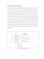
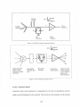
3 .4 .3 O p era tio n a n d D escrip tio n
The redesign of the interface involved primarily the simplification of its design but it
also involved the improvement of some of its physical construction characteristics to
improve reliability. One of the most obvious redesigns was in the reduction in the
number of Operational Amplifiers (Op-Amps) on the interface board. The number of
Op-Amps was reduced from four to two. Originally the board used two Op-Amps per
channel (i.e. two for each robot motor). The first Op-Amp in each channel decoded the
four bit string which contained the motors' direction and speed as per figure 3.2. This
configuration was a simple summing amplifier configuration as shown in figure 3.3.
Output from the summing amplifier was then passed to a power amplifier (Power-Amp)
circuit in order to boost the output to a level powerful enough to drive the motors on the
actual robot.
48
The reduction in Op-amps was implemented by setting up the summing amplifier across
the Power-Amp and removing the dedicated summing amplifier circuit across the
ordinary Op-Amp completely. The set up for the board was thus reduced in complexity
as well as reducing the number of connections (and thus the possibility of hardware
failure). The calculations involved in designing the summing amplifier configuration as
well as the final design of the interface itself are shown in Appendix D.
The original interface was also populated largely with potentiometers. These were
replaced with fixed resistors in order to increase the stability of the interface board. This
was because the potentiometers used in the original design were not of a very high
quality and they appeared, on examination, to have been damaged. This may have been
due to the fact that the board was not stored in any form of protective box. The
potentiometers used seemed to demonstrate a tendency to short-circuit themselves quite
regularly. This obviously affected the operation of the interface quite adversely by
changing the apparent motor responses to the input stimulus applied to the robot. This
situation made what were apparently identical neural networks behave in totally
different ways to the same stimulus and this uncertainty would have made it impossible
to effectively evaluate the behaviour of the robot later in the project.
It was also mentioned in the introduction to this section that the interface board was of a
wire-wrap configuration which was tidied up at the start of the project implementation.
As time progressed however it became obvious that this was unacceptable. Prompted by
the continual loosening of the connections, especially when coupled with the problems
associated with the potentiometers of the original design, it was decided to transfer the
49
circuit to a different and more stable medium. It was decided to used a vero-board
construction. This allowed a speedy construction and with the constituent parts being
soldered into place the entire construction is much more stable and physically secure.
Also the interface was improved by added a smoothing capacitor circuit to the power
input (see Appendix D).
3.4.4 Sum m ary
After discovering the failings of the original interface and its subsequent redesign and
reconstruction based on those findings the interface was a very stable and reliable
member of the hardware setup. The difficulties that were previously encountered did not
resurface again during the final stages of the project.
An advancement that could perhaps be made would be to finalise the design by
committing the interface circuit to a PCB format. However that would only really
become a consideration were the robot itself to become autonomous in the manner
suggested at the end of the section on the robot SBC. Obviously, the integration of the
SBC with the robot could not happen if the interface were not also integrated. Similarly,
integration of the interface alone would not be a very sensible step as it would not be
any advantage to the operation of the robot itself.
50
3.5 The Robot
3 .5 .1 G r o u n d in g s
As already mentioned already, the robot plays a vital role in testing and verification of
the neural networks grown using the phenotype development software (see section 4.4).
Also the testing of every change and every improvement on the physical robot before
advancement is at the crux of Brooks subsumption architecture approach, which the
project is attempting to implement. At the same time however, due the experimental
nature of the project, it would have been foolish to have designed a very sophisticated
robotic structure. It was rather more necessary to design a robot that would
be
physically flexible. It was impossible to predict exactly what problems could have been
encountered, problems which could potentially have forced a redesign.
It was hoped that any minor imbalances, such as a slight difference in motor
characteristics, could be compensated for by the neural network operation. In a sense,
hoping that a certain level of self-awareness would become apparent. The structure, in
particular the sensory bumper frame, did not appear to affect the mobility and operation
of the robot in its environment excessively, although a number of small problems were
encountered. These difficulties and their potential solution are detailed in section 3.5.
3 .5 .2 D e s c r ip tio n
The robot consists o f a number of parts which can be seen in figure 3.4. The individual
parts are the motors for the wheels, the micro-switches that act as sensors for the robot,
the sensor bumper frame to increase the activation area of the micro-switches and the
51
physical robot structure itself to hold it all together. The final part of the robot is the
cable connection between it and the interface board connecting it to the SBC.
The original robot parts were inherited from another project[21] run in the School of
Electronic Engineering in Dublin City University, and its basic design, which can be
seen in figure 3.4, remained largely unchanged over the course of the project. The robot
was constructed using constituent parts of a ‘LEGO Technics’ building blocks package.
This offered the ability to change system design quickly as well as allowing a prototype
robot to be built in minutes rather than weeks.
A number of enhancements were made to the inherited robot because, as the project
progressed, a number of problems became apparent. The first problem detected was that
the micro switch sensors used on the inherited robot were not sensitive enough to be
useful. The operating force required to close an individual switch was equal in
magnitude to the force required to move the robot physically from one position to
another. The sensors were thus replaced with micro-switches of a much lower operating
force. Also, they were glued to the robot framework to prevent them from slipping out
of position. Previously the sensors were attached using a small quantity of industrial
tape and under continued use they would slip from position. The replacement was
successful and the new sensors did not suffer the same problems as those that were
replaced.
52
15cm (app)
Plan viewofRobot
15 cm (app)
Robot
Legend
Back
of
Robot
Front
of
Robot
Sensor
0
Wheel
Frame
/ \
0 0 0 0 0
0 0 0 0
Side
Figure 3.4 The Robot
53
Connector
The cable connecting the robot to the SBC via the digital to analog interface had to be
replaced. The existing cable was unsatisfactory as it consisted of a number of individual
wires and was connected permanently to the robot. This connection’s soldering was
exposed and was prone to breaking. This cable was thus replaced by a 16 way ribbon
cable. Sixteen channels was more than what was required for the level of information
transfer between the robot and the SBC. However, the use of different sensor types, or
even expansion to the use of more than the existing six micro switch sensors already in
place, was being considered. The new cable was terminated by a 16 way D-connector.
This was advantageous as it meant that it could be disconnected from the robot when in
storage. The D-connector also reduced the risk of any damage which may have occurred
due to any twisting of the cable.
Next, a sensory bumper frame was constructed for the robot to increase the area that
each sensor covered. A frame of the shape shown in figure 3.4 was designed. This shape
was chosen because it is easy to construct and allowed continued operation with the
existent sensory layout on the robot. The frame was constructed using hard cardboard
allowing it to be replaced easily if it should become damaged. The frame worked well in
increasing the area that could activate the sensors.
3.5.3 Sum m ary
The robot satisfied its requirements physically. Its simple design was ideal for the early
stages of a project such as this. The use of LEGO building blocks in particular was very
successful in building the prototype. In the longer term however, a more robust robot
would necessarily be built. LEGO building blocks have a tendency to separate over
54
time. This affect caused the sensory framework to distort and become misshapen over
time thus preventing it from operating correctly until repaired. The largest problem with
this was that, as the LEGO separated and the frame became distorted, the edges of the
sensory frame flaps would occasionally become trapped against some corners of the
evaluation environment. This occurred particularly when the robot was performing
some form of circular motion (e.g. on reflex reversal from a wall while edge following).
The robot would then have to be freed manually and the frame adjusted. To improve the
framework and preventing a similar situation occurring a more comprehensive, flexible
and circular framework should be constructed in a form similar to that indicated in
figure 3.5.
Figure 3.5 Improved Sensory Framework
55
This new framework would prevent many of the physical difficulties described and also
provide a more comprehensive and operational sensory area.
•
•
#
3 *
A further beneficial enhancement would be the inclusion of a motion detector in the
sensor array. This would become useful when the robot becomes stuck in its
environment. The design of the controlling neural network could reward the generation
of random behavioural response when the robot becomes stuck. The motion detector
could operate in a number of ways, but the easiest would be to include some form of
current detector on the wheels’ motors. When the motors are prevented from turning,
(e.g. when the robot becomes stuck), the internal motor resistance is increased which
forces the current input to be increased. This detector could be incorporated onto the
robot/SBC interface board design.
1 Som e form o f m otor torque detector perhaps.
56
3.6 Behavioural Evaluation Environment
3 .6 .1 I n tr o d u c tio n
In this section a simple description of the environment in which the robot’s behaviour
was evaluated will be given. The environment was a very simplistic one which was
designed to test the ability of the networks generated to control the robot to prevent the
robot becoming stuck.
3 .6 .2 D e s c r ip tio n
The environment, as mentioned in the introduction to this section, was designed to test
the ability of the networks generated to satisfy the first level of Brooks’ subsumption
architecture specification^] . Namely, the desired behaviour of the robot was to move
around the environment and not become stuck. The environment is shown in figure 3.6.
The environment walls were constructed from LEGO building blocks. The environment
was 1.2m by 0.9m in size. A number of simple challenges were designed into the
environment to test the behavioural success of the robot in the environment. These were
as follows. Firstly a large open space to see if the robot would simply spin in circles if
there was nothing impeding its path (A). Secondly, a narrow channel was constructed to
see if the robot could reverse itself out such a gap, if it got itself into it(B). A couple of
‘rooms’ were constructed with only a single exit. The first of these was a large room
with a narrow exit. (C) The second was a smaller room with a single exit (D) and finally
a small room with an angled wall and a narrower exit(E).
57
1.2m
0.9m
Figure 3.6 Behaviour Evaluation Environment
58
3.7 Summary
The hardware used in the course of the project caused some significant problems which
were beyond the scope of this project to analyse fully. Rather it was more essential to
simply identify the causes of any such difficulties and come up with the most rapid and
effective solution to allow the project to continue. The failure of the original SBC used
is a prime example of such a situation. In general however, the hardware caused few
problems due to the simplicity of the overall design. The hardware, although essential
from the point of view of the project’s objectives, was essentially secondary with
respect to the theoretical aspects of the project. Certainly, any further exploration of the
area would require a significant increase in robustness and functionality (from the robot
in particular), but for a prototype framework, the hardware components were essentially
satisfactory. Any difficulties that did arise were dealt with quickly and efficiently
allowing the project work to continue without overly significant hindrances.
59
4. Software Implementation Details
4.1 Introduction
In this chapter all the relevant details, and where appropriate an analysis, of the software
components of the project will be presented. This includes descriptions of the overall
software environment (see section 4.1), source code and executable code considerations
(section 4.2). It also documents the implementation of the simple genetic algorithm
(section 4.3), the neural network growth software(section 4.4) and the neural network
simulator (section 4.5). Finally an overall summary of the software written (section 4.6)
is given. Also, recommendations for future improvements will be given at appropriate
points in the chapter.
The types of software used in the development of the experimental framework were
very varied. It consisted of high level code controlling the implementation of algorithms
based on existing natural systems. Assembly level functional code was used to control
the i/o ports for robotic control. Software was also used to implement remote machine
operation controllers using existing applications and a dedicated batch process. This
variability in software type was due purely to the diversity of functionality that was
required by each section of the hardware and the overall framework.
The main language that was used in the software development was C. This was for a
number of reasons. The first and most primary reason for this choice was that the C
language supports the implementation of both high and low-level code. This allowed the
60
relatively simple implementation of all the higher level algorithms. It also supports the
programming requisites for bit and byte level manipulation of strings. This bit-level
manipulation is visible in the i/o port configuration settings and readings on the robot
SBC as well as in the string manipulation of the genotypes used by the simple genetic
algorithm. The secondary reason for the use of the C language was my own familiarity
with the language. This familiarity applied both to the development platforms used as
well as with the level of software control that can be afforded by the C language
structure.
The development platforms used in the development of the C source code were the
‘Turbo
C++’
compiler/development
platform
and
the
Borland
C++
compiler/development platform packages. All the programs written were in standard C
format and did not exploit the capabilities of object oriented programming techniques.
The C language was used in development of the SGA, computational embryology,
computational neuroethology (neural network simulator) and artificial neural network
simulation software.
The secondary programming language that was used in the design framework was
MC68000 assembly language. This was the native language of the robot SBC.
Therefore, the neural network simulator software, which was written in C for the
reasons outlined above, needed to be converted to the 68000 assembly code for
implementation. This was achieved using the PARAGON C cross compiler package
whose operation is described in section 4.2.
61
A number of difficulties presented themselves over the course o f the project which had
significant effects on the programs as the development continued. These difficulties will
be documented in more detail later in this chapter. The problems were all overcome
however and, by the end of the project research period, the software being used was
both robust and reliable. Changes could of course be made to the final software to
improve both the performance and the functionality and some recommendations for
those changes are made in the summary of this chapter. However, I think that the results
obtained through the use of this software vindicates the choices and decisions made as it
was developed. These decisions and the final state of the software used will now be
described.
62
4.2 Paragon Cross compiler
4 .2 .1 I n tr o d u c tio n
The PARAGON C Cross Compiler [28] was used to convert the source code, written in
C, to the MC68000 assembly language. This conversion was necessary for execution of
the network simulator code on the robot SBC. The PARAGON cross compiler
supported the fundamentals of the C language. However the compiler caused some
difficulties as the differences between itself and the C compilation platforms used (see
section 4.2.2) for the source code generation became apparent. One of the areas in which
the differences can become apparent is in the manner in which the compilers handle
cross data type operations. This is because different compilers have different conversion
routines to deal with these situations. To illustrate one of these situations, consider what
happens when a real number is multiplied by an integer. Does the integer become
converted to a real number before calculation or it the real number converted to an
integer first? Over time however, these discrepancies were ironed out and the
PARAGON product proved itself able to satisfy the requirements made of it very
successfully.
4 .2 .2 O p e r a tio n
The operation o f the PARAGON C cross compiler was very simple. The software
written in C was simply used as an input. This software was developed and decoded
using a network simulation software package. The differences between the simulator
and simulation are described in section 4.5. For now, it is sufficient to know that the
simulation used the same core software as the simulator but also included a section that
63
mimicked the motor outputs and sensory inputs of the robot. Only when the simulator
code was at a point where it could be tested on the physical framework of robot and
SBC was the PARAGON C cross compiler was used.
The PARAGON Compiler software consisted of two separate programs. The first cross
compiled the C software and the second program assembled and linked it. The resultant
software was then downloaded to the FORCE SBC via the serial port of the PC using
the KERMIT software[29].
The cross compiler was a command line compiler which used a configuration file (see
Appendix A) to generate the assembly level code for the robot’s MC68000 FORCE
SBC. This configuration file was used to specify the areas of memory that could be used
for the executable code on the FORCE SBC. This configuration file also allowed the
specification of the format of output that could be produced by the compiler. This
included the production of memory mapping reports as well as full assembly listings
and S19 format file output[29].
4 .2 .3 S u m m a r y
The PARAGON C Cross Compiler software fulfilled all its functional requirements
admirably. Although not very pretty or easy to use, in comparison to the Turbo C++
development platform for example, it performed admirably. One advantage it had was
that the cross compilation procedure, once it was settled, could be operated using a
single command on the PC by using batch files. This meant that it simply did its job
64
with very little fuss, thus leaving the developer to concentrate on the code being written
rather than where it had to work.
65
4.3 Simple Genetic Algorithm Software
In this section o f the thesis the application o f Simple Genetic Algorithms (SGAs) to
neural network design will be detailed. More information regarding the operation of an
SGA and the genetic operators used in its operation can be obtained from section 2.4.
At the crux o f genetic algorithm operation lie what are called genetic operators. There
are three genetic operators used in the SGA. These operators are explained and
described in section 4.3.5. Some o f the C code which implements the genetic operators
is listed in this section.
There is also a section on the random number generator being used in the SGA (section
4.3.4).
Section 4.3.1 gives a brief re-introduction to SGAs and also deals with the reasoning
behind the choice o f simple genetic algorithms for the development o f neural networks.
How the basic SGA, outlined in Goldberg [14] (and in section 2.4), has been modified
for this project using the work o f Richard Dawkins[9,10,l 1] will also be detailed.
Dawkins' work is treated in more detail in section 4.4.
66
4.3.1 Introduction and R easoning
For convenience, the table outlining the terminology used in this section is reproduced
for the reader.
SGA
Simple Genetic Algorithm
Search Space
The problem space o f the simple genetic algorithm.
Genotype
Bit string which encapsulates the parameter set o f an individual.
Phenotype
Entity created from the decoding o f a Genotype. For this
application the phenotype is a neural network.
Individual
Refers to the Genotype and Phenotype as a single unit.
Fitness
Value assigned to individuals based on their performance. Used
in reproduction of individuals.
Population
A collection o f individuals.
Generation
A particular instance o f a Population.
Figure 4 .I Terms used in reference to Simple Genetic Algorithms
As discussed in section 2.4, the simple genetic algorithm is an optimising search
technique. It has been shown to be a useful tool in the traversal o f non-linear or complex
search spaces, particularly in applications that do not necessarily require a precise
solution, but do require a solution approaching the optimum. A neural network o f the
form being used in this project is one such application. Therefore, its implementation
within the design framework to guide the development o f a neural network to control
the robot is ideal.
Also, the simple genetic algorithm is based on a natural system. It draws its inspiration
from the apparent ability o f real genetic material, in the form o f DNA, to adapt to its
67
environment. As stated in the thesis introduction, one o f the aims o f this project was to
model natural systems as much as possible, within the confines o f the project, to achieve
its objective. The use o f the SGA satisfied this criterion.
The application o f the SGA is based on the PASCAL code which is documented in
Goldberg[14]. This allowed the algorithm to be applied very quickly and there was no
room for error in the translation from PASCAL code to C code simply because the
PASCAL code was very straightforward. There was only one major difference between
the SGA as laid out in Goldberg[14] and how it was applied to the development of
neural networks in this project. The difference lies in the fact that no explicit objective
function 4 is used within the course o f this project. Instead, fitness values are assigned to
the individuals by the network designer based on the rules documented later in this
document (see chapter 5).
Allowing the designer to assign the fitness values rather than using an explicit
evaluation/objective function resembles the work of Richard D awkins[9,10,ll],
Dawkins used just such a system to guide the development o f his ‘biomorphs’[9].
However, for this application it is not the shape o f the pictures produced which is
rewarded but the ability o f the neural networks produced to control a robot. Dawkins’
work and its application is described more in section 2.5 and in section 4.4.
4 See section 5.1.
68
The technical application of SGAs within the framework o f neural network
development will now be outlined.
4 .3 .2 A p p lic a tio n
The simple genetic algorithm works using a generation o f genotypes. The greater the
number o f genotypes, then the greater the chance that one will ‘fall’ close to a local
optimum in the search space. This hopefully will reduce the amount o f time necessary to
find a suitable optimum or solution in the search space. However, due to the time taken
to evaluate each genotype, it is necessary to reduce the number o f genotypes to a
manageable amount. This figure must also reflect the size o f the search space. For this
project the number chosen was initially ten in order to test the operation o f the SGA
programs. However, when the program was used within the design framework this
number was increased to twenty in order to increase the possibility o f discovering a
genotype approaching the optimum in the search space.
The twenty genotypes were generated by simulating the toss o f an unbiased coin. This
produced the first random generation o f genotypes. The random nature o f the first
generation distributes the SGA search’s starting randomly across the genetic search
space.
The genotypes themselves are binary strings o f 54 bits. Different sections o f the
genotype contain the coded parameters that are used to grow the neural networks. The
details o f this growth are given in section 4.4.3. As described in section 2.4 of this
69
project, SGAs operate on a coding 5 o f a systems parameter set and not the parameters
themselves. The specific coding o f each genotype used in this project is shown in
section 4.4.6.
One by one each of these randomly generated genotypes is decoded by the
d e v e l o p m e n t program (see section 4.4) and a network is generated or 'grown' using
these decoded parameters. The neural network produced by the network development
program is then downloaded onto the MC68000 FORCE board where the network
simulator has already been loaded into the MC68000 FORCE board's memory. The
simulator is run and evaluated by the network designer. Each network is examined on
how the robot responds to its environment and a fitness value (which is an integer in the
range 10 to 100) is awarded to the network based on its level o f success. The better the
robot responds then the closer to 100 the assigned fitness value should be.
When all the networks within the generation have been evaluated, the SGA program is
run on the PC to create the next generation o f 20 genotypes. To do this the designer is
prompted for the fitness value that was assigned to each o f the networks. The old
population and the fitness values o f each o f the genotypes are then used to generate the
new population using the crossover, mutation and reproduction genetic operators. A
detailed description o f the operation and the coding o f these genetic operators is given in
section 4.3.5. In brief however, these operators are at the heart o f the operation o f the
5 The description and relevance o f each o f these parameters is explained in section 4.3.5 w hich deals w ith the
d e v e l o p m e n t program. F o r now it is only important to know that the coding used generates a string o f 54 bits.
E ach bit represents part o f a parameter used by the d e v e l o p m e n t program to grow a neural network . Each bit
can assume the value ' I 1or 'O' only.
70
SGA allowing the production o f the next generation based on the performance of the
last. This process o f testing and evaluation is continued until the algorithm finds a
network suitable to control the robot.
4 .3 .3 G e n e tic C o d in g B r e a k d o w n
h
21
25
_L
31
39
I
50
44
I
i n i n i i i n n m n 11 n n
rn
54
i
i
1
I/O Configuration
Inhibition Code —
Link Growth Rate
Division Rate
Number of Cycles
Generator Ratio _
Division Distance
Number of Outputs
Figure 4.2 Coding o f Genotypes Produced by Simple Genetic Algorithm
As mentioned above, the genotypes are 54 bit binary strings. The genotype can be
thought o f as being a concatenation o f a number o f smaller binary strings. Each smaller
string representing one o f the variable parameters used in the development and
operation o f the neural networks used for controlling the robot. The relevance o f each of
the parameters is detailed in section 4.4.6. A diagram o f the genotype is shown in figure
4.2.
71
4.3.4 R andom N um ber G eneration
Random number generation is used throughout the operation o f the SGA. It is used in
the initial distribution o f the genotypes across the search space. It is also used in the
selection o f individuals from each generation, based on their performance scores, in
order to create the next generation of genotypes. Earlier in the project, the C random
number generation routines were used. However, based on advice received regarding the
performance o f these functions, a different random number generation routine suite was
adopted.
The full suite o f routines can be seen in Appendix C o f this document.
Four o f the routines were called from the software used in this project. The routines
were called G etO neJU niform , Get One Bernoulli, Get Msr 88 and Set_SeedMsr 88.
The code segments for these routines are now shown for completeness.
p u b lic
flag
g et_ o n e_ b ern o u lli(d o u b le
p)
{
in t3 2
cut
= MSR88_RANGE;
if
( v a l i d _ f r a c t i o n ( p ) ) c u t = f r o u n d ( p * (double)(M SR88_RA N G E)) ;
e ls e p a n ic (" g e t_ o n e _ b e rn o u lli: In v a lid param eter <p>!");
r e t u r n ( g e t _ m s r 8 8 ()
< c u t);
J ________________________________________________________________________________________________
Figure 4.2 Get One Bernoullif)
72
p u b lic
in t3 2
g et_one_uniform (int32
n)
{
int32 c u to ff
s t a t i c int32
= MSR88_RANGE;
v;
if
( ( n >= 1 ) && ( n <= MSR8 8 _ R A N G E ) )
c u t o f f = (M SR88_RANGE/n) * n ; / * S e e n o t e i n
e l s e p a n i c ("g et_ o n e_ u n ifo rm : I n v a lid p a ra m e te r
do v = g et_ m sr8 8 () ;
w h i l e ( v >= c u t o f f ) ;
retu rn (v
/*
See
n o te
in
g e t_ u n ifo rm ().
<n>!");
g e t_ u n ifo rm ().
*/
*/
% n );
J __________________________________________________________________________________________________
Figure 4.3 G etO n eJJn iform O
p u b lic
in t3 2
g et_m sr88(void)
{
s ta tic
s ta tic
in t3 2 t e s t ; /*
ld iv _ t lohi;
c o u n t ++;
if
(count
s ta tic
for
s p e e d ...
*/
>= M S R 8 8 _ R A N G E )
{
w a r n ("get_msr88: count >= MSR88_RANGE!");
count = 0;
}
lo h i
= ldiv(seed,
Q );
t e s t = A * l o h i . rem - R * l o h i . q u o t ;
if
( t e s t > 0) s e e d = t e s t ;
e l s e s e e d = t e s t + M;
re tu rn (s e e d -1);
2__________________________________________________________________
Figure 4.4 Get_Msr88()
p u b lic
v o id
set_seed_m sr88(int32
new seed)
{
if
( ( n e w s e e d >= 1 ) && ( n e w s e e d < = M S R 8 8 _ R A N G E ) )
seed = new seed;
e l s e w a r n ("m sr8 8 _ s e t _ s e e d : i n v a l i d <new seed> p a r a m e t e r ! " ) ;
_}______________________________________________________________________________________
Figure 4.5 Set_Msr88()
73
4.3.5 SG A O perators
It has already been stated that the genetic operators lie at the heart o f the operation o f the
SGA. In this section each o f the three operators implemented in this project will be
described and its role in the operation o f the SGA documented. The three operators used
are the reproduction operator, the crossover operator and the mutation operator. Each o f
these operators uses the random number generation routines described above in section
4.3.4. The implementation o f the random number generation will be described, with
reference to each o f the operators, in this section. The C code implementing these
operators will also be shown for completeness.
4.3.5.1 The Genotype Selection Function
Shown below in figure 4.7 is the select () function that selects candidates from a
population for mating based on the fitness values assigned to individuals. It is based on
the PASCAL procedure select in Goldberg's book[14][p. 63].
74
in t
* select(d o u b le
pair_num ber)
{
in t
in t
in t
double
in t
if
((m ates
j =0 ;
i= 0;
ro u lette= 0 ;
partsum = 0;
*mates=NULL;
= m a l l o c ( 3 * s i z e o f ( i n t ) ))
= = NULL)
{
p r i n t f ( "N ot
enough
mem ory t o
e x i t (1);
/ * T E R MI N A T E PROGRAM I F
allo cate
buffer
{fn
s e l e c t ()}
\n " );
OUT O F MEMORY * /
}
f o r ( i = 0 ; i < 2 ; i++)
{
ro u le tte = (in t)(ra n d o m _ flo a ts[i+ (p a ir_ n u m b e r* 2 )]*
to ta l_ g en etic_ fitn ess);
/ * VALUE CHOSEN WHICH D E T E R M I N ES WHICH CHROMOSOME
OF
/ * THE OLD P O P U L A T I O N
TO CROSS (OR NOT) WI TH ANOTHER
/ * OLD CHROMOSOME.
/ * S E E GOLDBERG FOR D E T A I L S
*/
*/
*/
*/
f o r (j =0 ; j <MAXPOP_SIZE; j + + )
{ '
i f ( ( p a r t s u m += o l d _ p o p u l a t i o n [ j ] . f i t n e s s ) > r o u l e t t e )
break;
i f ( j = = M A X P O P _ S I Z E - 1)
break;
}
* (m ates+ i)= j;
partsum = 0;
}
retu rn (m ates);
}
Figure 4.6The SGA SelectQ Function
The s e l e c t () function uses a pre-constructed array (random_floats) to select a value
(X) which lies between 0 and the sum o f the assigned fitness values o f all the
individuals in the population. The function then iterates through the population index,
adding each individual's assigned fitness value to a temporary sum figure(Y) which is
initially zero. When the temporary sum figure(Y) exceeds the randomly generated
number(X) then the individual responsible for the last addition to (Y) is selected for
75
reproduction. What this means is that the higher an individual's fitness figure is, then the
higher the chance that the addition o f that particular individual's fitness figure will result
in the randomly generated number(X) being exceeded by the temporary sum(Y), and
hence be an individual picked for reproduction. This operation is described by Goldberg
using a roulette wheel analogy[14] which intuitively may be easier to understand than
this purely textual description.
The reproduction operator is an artificial version o f natural selection, a Darwinian
survival o f the fittest among string creatures. In natural populations, an individual's
fitness figure is determined by its ability to avoid disease, predators and other obstacles
to adulthood and subsequently mate. In this artificial setting the fitness figure is the sole
arbiter for the survival o f the string creatures.
This function is called twice within the user defined function c r o s s o v e r () (see
4.3.5.3) to select a pair of individuals for breeding. When two distinct individuals have
been selected then the crossover between the genotypes is carried out within the
c r o s s o v e r () function.
4.3.5.2 The M utation Function
Shown in figure 4.8 below is the code which implements the mutation function. This
function is also based on the equivalent Pascal procedure in Goldberg[14][p. 65],
Within a simple genetic algorithm implementation the mutation and crossover operators
can be used either mutually or exclusively. For example, Dawkins’ implementation in
76
the creation o f his biomorphs[9] does not use the crossover operator at all. Instead he
depends purely on a mutation operator and a reproduction operator. In this
implementation, both are used.
in t
m u tatio n (in t
single_gene)
{
in t
m utate
if
new_gene;
in t
m u tate;
= flip(PRO B_M UTA TATION );
/ * F L I P S I M U L AT E S A WEI GHTED C O I N T O S S AND I S U S E D
/ * HERE TO DE T E R M I N E WHETHER A S I N G L E B I T SHOULD BE
/ * MUTATED OR N OT . F L I P U S E S THE G E T _ O N E _ B E R N O U L L I ()
/ * FUNCTION
*/
*/
*/
*/
(m utate)
{
tex tco lo r(R E D );
if
( s i n g l e _ g e n e == 1)
new__gene = 0 ;
else
new_gene = 1 ;
}
/*
IF
/*
Q U E S T I O N I N THE CHROMOSOME I S
THE F L I P
F U N C T I O N RETURNS A
'1 '
THEN THE B I T
I N V E RT ED
IN
*/
*/
else
new_gene
# if
= sin g le_ g en e;
DEBUG
m utate_num ber+ + ;
#en d if
retu rn (n ew _ g en e);
/ * RETURN THE VALUE OF THE NEW B I T
}
Figure 4.7 Implementation o f the SGA Mutation operator
The mutation operator in this implementation is present purely to prevent important
information being lost. This can happen as the SGA population begins to approach an
optimum solution in the search space. As the optimum is approached, all the genotypes
begin to resemble each other. This is fine, as that is what the SGA is supposed to do.
However, if one is dealing with a search space which has more than a single optimum,
77
the SGA could be converging on a local optimum rather than the search space optimum.
This concept o f multiple optimums is explored in more detail in GoIdberg[14], What the
mutation operator does is to change, at random, small parts o f individual genotypes. If
used correctly6, the operator can act as an insurance policy for the SGA, potentially
preventing it from converging on a local optimum, rather than the search space
optimum.
The coding implementation o f the operator is simple once the mutation rate for the
population has been chosen (see section 4.3.5.4). In the crossover function, each bit of
each genotype is passed into the function m u t a t i o n ( ) . The random number function
f l i p () is then used to decide whether or not the bit is to be mutated. The probability
o f mutation is passed as a parameter t o
f l i p ( ) , as it is also used to select a crossing
site for parents in the crossover function.
4.3.5.3 T h e Crossover Function
The c r o s s o v e r () function (see figure 4.9) implements the crossover operator. It uses
the results o f the s e l e c t () function as two o f the input parameters. It also uses the
m u t a t i o n () function internally to implement this form o f crossover. It is based on
the equivalent PASCAL procedure in Goldberg[14][p. 64]. A thing to note is that the
function does not allow generations to overlap. This means that genotypes from the old
population (from whose parts the new generation is constructed) may not cross with the
6 T h e c h o ic e o f g e n e tic o p e r a to rs ca n b e b ia s e d w ith in a n y p a r tic u la r a p p lic a tio n to w h ic h e v e r th e d e s ig n e r c h o o se s.
F o r e x a m p le in D a w k in s ’ w o r k , th e m u ta tio n o p e ra to r is u se d to th e e x c lu s io n o f th e r e p ro d u c tio n g e n e tic o p e ra to r
[9].
78
new generation's genotypes during the creation o f the new population o f individuals.
The reasoning behind this choice was to make the implementation o f the SGA as simple
as possible. As was mentioned before, with reference to the biasing o f genetic operator
influence, the crossover function can also be made much more complex. It can, for
example, involve cross generation coupling as well as self reproducing genotypes if
required.
79
v o id
{
c ro s s o v e r(in t m a te l,in t m a te 2 ,in t cro ssp o in t)
int cross;
int xsite;
int iter;
int parentl[GENE_LENGTH] ; int parent2[GENE_LENGTH] ;
f o r (iter=0;iter<GENE_LENGTH;iter++)
{
parentl [iter]
parent2 [iter]
= old_population[matel] .chromosome[iter] ;
= old_population[mate2].chromosome[iter];
}
/* GET THE TWO CHROMOSOMES CHOSEN FOR REPRODUCTION O R * /
/* CROSSINGFROM THE OLD POPULATION RECORD
cross = f l i p (PROB_CROSSOVER);
/* FLIP SIMULATES A WEIGHTED 'COIN TOSS' AND IS USED
/* HERE TO DETERMINE WHETHER THE TWO CHOSEN
/* CHROMOSOMES SHOULD BE CROSSED TOGETHER OR NOT
*/
*/
*/
if (cross)
{xsite = crosspoint;}
else
xsite = GENE__LENGTH ;
/* IF THE CHROMOSOMES ARE NOT TO BE CROSSED THEN THE
/* CROSSING SITE CHOSEN IS SIMPLY THE END OF THE TWO
/* CHROMOSOMES.
*/
*/
*/
gotoxy ( x s i t e + 7 , (popsize*2) + 4);
p r i n t f ( " x " ) ; /* PRINT POSITION OF CROSSING SITE ON SCREEN
*/
for
*/
(i t e r = 0 ;i t e r<xsite;iter++)
{
textcolor(GREEN);
new_j?opulation[popsize].chromosome[iter] = mutation(parentl[iter]);
gotoxy(iter+7,(popsize)+3);
c p r i n t f ("% d " ,new_jpopulation[popsize].chromosome[iter]);
textcolor(WHITE);
new_population[popsize+1].chromosome[iter] = mutation(parent2[iter]);
gotoxy(iter+7,(popsize)+4);
c p r i n t f ("% d " ,new_population[popsize+1] .chromosome[iter] ) ;
}
/* THIS LOOP GENERATES TWO NEW MEMBERS OF THE
/* POPULATION AND AS EACH BIT OF THE NEW CHROMOSOMES
/ ♦ I S GENERATED BY THE CROSSING IT IS DETERMINED
/* WHETHER OR NOT IT SHOULD BE MUTATED
*/
*/
*/
*/
i f (xs i te != GENE J L E N G T H )
{f o r (iter=xsite;iter<GENE_LENGTH;iter++)
{
textcolor(WHITE);
new population [popsize] .chromosome[iter]=mutation(parent2[iter]);
g otoxy (iter+7, (popsize)+3)
c p r i n t f ("%d",new_population[popsize].ch r o m o s o m e [iter]);
textcolor(GREEN);
new p o pulation[popsize+1].chromosome[iter]=mutation(parentl[iter]);
g o t o x y (iter+7, (popsize)+4);
c p r i n t f ("%d",new_population[popsize+1].chromosome[iter]);
g o t o x y (5,popsize+3);
}
}
/+
/*
/*
IF THE CHROMOSOMES HAVE BEEN CHOSEN FOR CROSSING
THEN THIS WILL IMPLEMENT THE ACTUAL EXCHANGE OF
BITS. IF NOT, THEN THE PROGRAM WILL NOT ENTER THIS LOOP.
*/
*/
*/
)___________________________________________________________________
Figure 4.8Function in C to implement the crossover operator
80
4.3.5.4 Genetic Parameter Choices
So what values were chosen for the probabilities o f crossover and mutation occurring?
To choose these numbers, the work o f Goldberg was again addressed. Goldberg
references a study by De Jong [12] in the application o f genetic algorithms to function
optimisation. He states that De Jong recommends the choice o f a high crossover
probability coupled with a small mutation probability (inversely proportional to the size
o f the population) and a moderate population size [14]. Following these suggestions, the
following figures were chosen:
Probability o f Mutation:
0.01
Probability of Crossover:
0.9
Population size:
20
Figure 4.10 Genetic Parameters Used
These figures were chosen to allow the SGA to converge quickly (even to a local
optimum) to demonstrate the viability o f the overall design approach.
4.3.6 Summary
The Simple Genetic Algorithm was an adequate choice for the project. It is entirely
possible o f course, that there is a different form o f the genetic algorithm that would be
even more suited to artificial neural network design. However, as has already been
explained, only the briefest examinations could be made o f each o f the theoretical areas
employed due to the time scale of the project. The implementation o f the SGA was
aided by the conscious decision to avoid over-complication o f the core code. The
81
operation o f the code itself was validated early in the project[25J. The working o f the
final code in optimising the operation o f the neural networks is discussed in detail in
section 4.5 and thus will not be addressed here. However, it would be appropriate to say
at this stage that the operation o f the SGA code was a success with respect to the results
obtained.
82
4.4 The Network Development Program.
4.4 .1 I n tr o d u c tio n
After the manipulations o f the simple genetic algorithm, the network development
program decodes the genotypes created by the SGA. It uses the decoded genotype
parameters to create or 'grow' artificial neural networks. This growth process is
deterministic. It is based on some very simple rules that use the growth parameters
encapsulated in the genotypes.
This section details how these network growth parameters are decoded from the
genotypes. It also describes the Riles governing the creation o f a neural network based
on these parameters.
The inspiration for this approach is the work of Richard Dawkins [9,10,11], whose work
is in this general area, is also outlined in section 2.5.
83
4.4.2 O rigin o f the Idea.
As stated in the introduction o f section 4.4, the idea o f growing a neural network is
based on the work o f Richard Dawkins [9,10,11]. Dawkins' work in this project has
*
q
been emulated but instead o f re-creating Dawkins' biomorphs , neural networks were to
be grown. To accomplish this a set o f rules had to be constructed governing how the
neural networks were to be grown from the genotypes. These rules were constructed in
such a way as to attempt to make the growth o f the neural networks somewhat
biologically inspired. This o f course, is not the only way in which the development of
the neural networks could be done. In Sussex University a research team have
implemented a low level behaviourally based robot. However, instead o f using a growth
mechanism, such as in this project, they coded every connection in the neural network
into the genotype. Further details o f their work can be found in [6,7,8,15,16,17,18,20].
As well as defining the rules for growth, it was also necessary to decide what parameters
were to be encoded in the genotypes in order to facilitate this biological approach..
These parameters would be used by the rules to grow the networks. The rules used are
listed in section 4.4.3. These rules have been used successfully to generate a neural
network for robotic control. However, as with all areas o f this project, simplifications
were made in order to precipitate the implementation success. These simplifications
generated some problems and these problems will be discussed in this section where it
is relevant to do so.
7 Biom orphs are what D aw kins calls his biologically inspired pictures.
84
4.4.3 H ow D oes It W ork? (The R ules).
As stated above, a number o f rules were devised in order to make the growth of a neural
network from a genotype possible. These rules resulted in the growth o f the neural
network being deterministic and hence repeatable. It was a conscious decision to make
the growth a deterministic process as repetition o f the results obtained was very
important at this early stage. It was important to qualify any results obtained to validate
the procedure being implemented in the project. The rules will now be presented. The
rules have been broken down into three groups to make them more readable. The first
group describes the general rules governing the overall operation o f the growth process.
The second and third groups deal with the growth o f links between nodes and the
generation o f the nodes themselves respectively.
4.4.3.1 G eneral Rules
1.
The neural networks are made up o f two parts: nodes and
2.
The nodes are o f the types described in section 4.5.5.
links.
3. Links grow to form connections between nodes.
4. The networks are grown on a growth 'grid' o f size 255 x 255 units.
5. Each node occupies 1 unit on the grid and remains set in that position.
6. Each node can only attempt to create a connection with one other node at a time (i.e.
only has one link growing at a time).
7.
The position o f each node and link is stored as a set o f (x,y) co-ordinates
on the grid.
8. Six nodes exist initially on the grid in fixed locations, though not in fixed order.
Four of these are input nodes that represent the physical connections to the robot's
85
sensors and two are output nodes that represent the connections to the robot's
motors. Which node corresponds to which sensor or motor is determined by a
decoding o f the genotype.
4.4.3.2 Link Growth Dynamics
1. The current link (only one link grows at a time) o f a node grows towards the nearest
node relative to the tip o f the current link that is not the node from which the link is
growing - referred to as the parent node.
2. On each growth cycle the location o f the nearest node is re-evaluated. This reevaluation is to allow for the placement o f new nodes due to node division.
3. The link growth rate is constant for all links and is defined by the genotype.
4. Nodes can only connect (via the links) with a range o f 1 to 10 other nodes as defined
by the ‘number o f outputs’ growth parameter. (See figure 4.10).
5. When links do make a connection between nodes, the distance between the base
node and the newly connected node is the magnitude o f the weight of the connection
between the nodes as used in the simulator (maximum value 255).
6. The sign o f the connection weights is determined by decoding the genotype to
determine if the connection is an inhibitory link or not. This is defined by the
inhibition code parameter which is described in section 4.4.6.
4.4.3.3 Node Division Dynamics
1. Node division takes place at a constant rate to produce new nodes. This rate is
defined by the Division Rate parameter. See section 4.4.6.
86
2. Each node can divide once to produce only a single offspring, and the parent node
may continue to grow links after divisions up to the allowed maximum.
The positioning o f newly created nodes, on division from the parent node, is determined
by the following rules:
1. The division distance is constant for all node divisions and is decoded from the
genotype. This is defined by the Division distance parameter.
2. The division direction is determined by finding the nearest two nodes relative to the
parent node and finding the point that lies half way between them. See figure 4.11
for an illustration.
3. The position at which the new node is placed is at the division distance away from
the parent node in the direction o f the point derived above.
4. If the position o f the new node lies outside the growth grid then the new node is
placed within the growth grid. This is accomplished by determining which o f the
new node's co-ordinates has violated the boundaries o f the growth grid. The
offending co-ordinate is then adjusted so that it is brought back within the
boundaries o f the growth grid.
5. If the position calculated for the new node is within a radius o f 30 units o f another
node then the division is deemed to be invalid and the new node is not created. This
is to prevent 'clustering' of nodes in small areas of the growth grid. It was decided
that clustering could have prevented connections being made between the input and
output nodes. It was decided that this was best avoided at this early stage o f overall
framework development.
87
Parent Node
O
Line indicating Node Division
distance.
This Line bisects the line (A) between
the two nearest nodes
{
Two Nearest Nodes
to the Parent Node
on the Growth Grid.
«------ Position o f New Node
Line (A) connecting the two
nearest nodes by their centers.
Figure 4.9 Illustration o f node division dynamics.
4 .4 .4
I m p le m e n ta tio n o f th e R u le s
Implementation o f these rules within the development program produces 3 different sets
of data (arrays) as a final result. The arrays are:
1. An array to record the position o f every node on the grid.
2. An array to record all connections between nodes.
3. An array to record the connection weight between every pair o f connected nodes.
These three arrays are then combined and the format o f the combined array is adjusted.
The new format is adjusted such that the single final array contains all the information
8
*
in the format required by the neural network simulator and simulation software. This is
the array which is downloaded onto the MC68000 SBC and then tested on its ability to
control the robot. See chapter 5 for the behavioural evaluation rules. It takes a slightly
8 A n explanation o f the differences between the neural network simulator and simulation software, and the uses o f
the simulation software in the overall fram ework is given in section 4.5.
88
different form when being used in the simulation software. An number o f examples of
how the grown networks ‘looked’ are given in Appendix E. The download o f the single
formatted array will now be described.
4 .4 .5 N e tw o r k D o w n lo a d
The download o f the network to the MC68000 SBC is a simple operation. The
PARAGON C cross compiler[2 8] used to generate the simulator code also generates a
memory map listing the location o f all functions and global variables/data structures.
When the simulator code and the SBC are working correctly then re-loading o f the
simulator software is unnecessary within each generation evaluation run. This is because
the memory locations o f the variables, data structures and functions remain fixed. Hence
every network grown by the development program can be downloaded and slotted into
the same memory location to be used by the simulator already loaded in the MC68000
SBC's memory.
To allow the network download to the MC68000 SBC to be performed it was necessary
to write a C program which generated a file containing the network information in S I9
format [28]. This is the format required by the MC68000 SBC’s operating system to
allow recognition o f the incoming data. Use o f the S I9 specification requires the
development program to perform conversion o f the integer figures produced by the
development program to hexadecimal character format and the calculation o f checksums
and address offsets. The checksum calculated allows the MC68000 SBC to check if
download data integrity has been maintained. The offset generated is used to inform the
89
MC68000 system o f where to store the information in memory so that the simulator can
access it correctly.
Reference was made earlier in this section to the neural network simulation software. To
use the information from the development o f the network in the simulation program a
slightly different approach is taken. The PC on which the simulation is run does not
require S19 format downloads. The development program grows the network in the
same way and reduces the three arrays to the format required by the simulation and
simulator software. Then it outputs this array as a text file before the conversion to S19
format is carried out. This text file then contains the array information in the format that
the simulation software requires. The array is read directly from this file by the
simulation program.
To allow this difference in information transferal between the simulation and simulator
software, the development program has two separate versions. They are each contained
on the disk accompanying this report. The programs are called PCDEV.EXE which
produces the networks for the simulation software and DEVEL.EXE which produces the
S19 format file (through use o f the FORMS 19.C program) for download to the
simulator on the SBC.
In the next section the mechanism for the decoding o f the genotypes produced by the
SGA to grow the networks will be described.
90
4.4.6 T he G en otype Param eter D ecoding.
The SGA works on a coding o f a parameter set, not the parameters themselves. This
section deals with how these genotype parameters are decoded and what they represent
to the development program.
The decoding o f some o f these parameters is simple and the decoding o f some is not so
straightforward. The creation o f the final format in which the parameters have been
coded in the genotype was a gradual process. A number o f decisions had to be made
with regard to what exactly should be coded into the genotype. The most difficult area
to decide this in was with regard to the parameterisation o f the individual nodes within
the neural network. The neural nodes have a number of internal parameters which
directly affect their performance. It was decided to minimise the parameterisation o f the
nodes in order to reduce, as much as possible, the size o f the genetic search space. It was
hoped that this reduction in variability would facilitate a more speedy convergence to
some optimum on the search space. This convergence would then, hopefully, validate
the operation o f the design framework. The full details and reasoning behind this
reduction in variability will be given in section 4.5.4.
Shown below is figure 4.12 which has been reproduced for convenience to show the
location and name o f the different parameters that are coded within each genotype
produced by the genetic algorithm.
91
11
21
25
31
39
44
50 53
JL
J___ I
I/O Configuration
Inhibition Code
Link Growth Rate
Division Rate
Number of Cycles
Generator Ratio
Division Distance
Number of Outputs
J
Figure 4.12 Coding o f Genotypes Produced by Simple Genetic Algorithm
How the individual sections are decoded from the genotype is now listed parameter by
parameter
1. I/O configuration: Bits [1-11]. This parameter determines which sensor is placed in
which position on the growth grid. The algorithm can be observed in the function
in t
* g e t _ i o _ p o s i t ( i n t ) in the GET DATA.C program. The algorithm is
quite simple in nature. It uses the bits 7-11 to select the first node to be placed on the
g rid (l- 6). The remaining bits determine the order in which the remaining nodes will
be placed on the grid.
2. Inhibit Code: Ten bits [12-21] which determine which links are to be positive and
which are to be negative. A maximum o f ten connections is allowed so one bit
corresponds to each link. If the bit is a 1 then the weight is positive. If the bit is a 0
then the weight is negative.
92
3. Link growth rate: The bits [22-25] are translated into an integer between 1 and 16.
This is the distance which links grow in a single iteration o f the development growth
routine. It is possible that with a growth distance o f 1 that the link head position will
be the same after calculation as the current position o f the link head. This is caused
by rounding errors. To overcome this, the result is analysed and if the error is
detected the growth distance is increased to 2 units and recalculation takes place.
4. Node division rate: The five bits [26-31] are converted into a decimal integer
between 1 and 16. This number is multiplied by 10 to give a range o f 15 numbers
between 10 & 150. This is the number o f iterations o f link growth that occur
between node divisions.
5. Num ber o f Growth Cycles: The eight bits [32-39] are translated into a decimal
integer between 1 and 256.
6. Generator Ratio: The 5 bits [40-44] are used to determine which nodes act as
generator nodes 9 . The ratio can be between one in every 2 to 33 nodes.
7. Node division distance: The four bits [45-49] are first translated into a decimal
integer between 0 and 15. This number is then multiplied by 4.375 10 and 30 is added
to the result. This means that the division distances can take one o f sixteen numbers
between 30 and 100 units.
8. Number o f Outputs: The four bits [50-53] are used to indicate how many outputs
which each node can have. Ranges from 1 to 16.
9 See section 4 .5 .5 .2 for description o f the operation o f generator type nodes.
10 T h is factor converts the binary number distribution from the range 0-15 to 0-70.
93
4.4.7 N etw ork G row th.
The main function that controls the growth o f the neural network using the decoded
parameters is shown here as it is the most concise way of describing its operation.
vo id
sim _ g ro w th (in t
ax _ g rt,in t
d iv _ rt,in t
d iv _ d s,in t
* in b t,in t
num _cycles)
{
i n t count= 0;
in t iter= 0 ;
c h a r typ e;
c h a r m s g [2 0 ] ;
w h ile
(ite r
< num _cycles)
{
/* p a s s in l i n k g ro w th r a t e and i n h i b i t
g r o w _ l i n k s (ax__grt, i n b t ) ;
if
(c o u n t > = d i v _ r t )
/* i f tim e f o r node d i v i s i o n th e n b e g in
in fo rm atio n
*/
*/
{
i f
/* l i m i t on number o f nodes
(n u m _ n o d e s > ( MAX_NODES- 6 ) )
s t a l l () ;
/* f u n c tio n
to
ex it
program
allow ed
*/
g racefu lly
*/
else
grow _n o d es(d iv d s);
c o u n t = 0;
}
c o u n t ++;
ite r+ + ;
}
Figure 4.10 Controlling Junction fo r Network Growth.
Some o f the basic graphics functions that are included in the C libraries available to the
Borland and Turbo C++ compilers were used in the development program to allow
visualisation of the program's operation during debugging. This graphics element is
maintained within the program as it shows the person using the program that something
is happening while the network is being grown. This, I feel, is preferable to leaving the
screen blank and giving the user no indication that a network is or is not being grown
successfully.
94
4.4.8 Sum m ary
So why were these particular rules used, and how has the development program
performed? A number o f decisions needed to be made regarding this particular question
as the project progressed. Some o f the potential decisions were raised in 4.4.2 and in
this section these proposals will be reviewed and others that presented themselves at a
later stage addressed also.
One o f the first decisions was in reference to the node division mechanism. It had
previously been thought that the use o f the two nearest nodes relative to the node about
to divide to decide the direction in which the new node should be placed may not have
been good. It was thought that this method could lead to a situation where if the node
division distance was small then when the time comes for the new node to divide, it will
attempt to place its child node in the exact position o f its own parent. This, it was
thought, would minimise the number o f nodes which could occupy the growth grid even
when a lot o f grid space remained unfilled. The maximum number o f nodes that can
occupy the growth grid (assuming a minimum radius o f 30 units between all nodes) is
64. In the testing done to maximise the number o f nodes in a grid the maximum that
could be reached using the SGA was 25. On first glance this would seem to confirm the
worries highlighted earlier. It was thought that a change to select perhaps the 2n^ and
3rd nearest rather than the 1 st and 2 n^ nearest to derive the node division direction may
have unleashed more o f the growth potential. However, it was decided to trust in the
95
operation o f the SGA. Indeed, as the results appear to confirm (see chapter 6) this was a
vindicated choice.
It was also thought that it may not have been good to have the location o f the initial
nodes static on the grid. It was decided to allow this variability in the genotype coding
and to use the SGA to 'find' the best location for the opening configuration. The results
on this point were a little more difficult to evaluate. This point is discussed in more
detail in the conclusion.
Another parameter which made its appearance late into the project was the introduction
o f the generator nodes ratio. It was decided to use generator nodes to enable the system
to generate neural networks which would not require an external stimulus in order to
begin to operate. It was decided instead that some form o f spontaneous operation would
be preferable to kick-starting every network. This was because the entire operation and
biasing o f the network could have been determined by which external sensor was
stimulated first.
96
4.5 Simulator and Simulation
4 .5 .1 I n tr o d u c tio n
In this section the operation o f the neural network simulator and simulation software
will be documented. The simulator software was used to implement the artificial neural
networks that were created. It was designed to operate on the SBC controlling the robot.
The simulat/o« software was used to debug the simulator software by emulating the
operation o f the SBC on the PC. This allowed the neural network software to be
evaluated without the framework hardware considerations that have already been
documented in this thesis (see chapter 3) influencing or impeding its development. A
number o f difficult situations arose over the period o f development o f the simulator
software. Some o f these problems have already been referred to in previous sections the genotype coding and operation o f the SGA affecting the level o f parameterisation
possible for the neural nodes for example. Difficulties caused by the differences in
compilers (Borland C and Paragon C Cross Compilers) occurred. Other difficulties
arose prompting decisions about the operation o f the network based on initial results.
All these difficulties affected the overall development o f the software from its original
aspirations up to its final state. In this section o f chapter 4 the more difficult problems
encountered and their eventual resolutions will be documented.
Also in this section, the operation o f the neural networks will be described in some
detail. Reference will be made to the work o f Randall Beer[2] where appropriate. This is
because it was intended to use the type o f networks modeled by Beer to control the
robot. Beer’s network model was the ideal originally, but as the problems mentioned
97
above revealed themselves, it became necessary to make some quite significant changes
to the network morphology and operation. As much as possible however, Beer’s model
was adhered to. The eventual mechanics o f the connections allowed between nodes and
the various types o f nodes possible at the end o f the research period will be described.
As the operation of the networks is integral to the success o f the project, the operation of
the networks will be described first. Comparisons to Beer’s model will then be made.
4 .5 .2 O p e r a tio n o f th e N e u r a l N e tw o r k .
So how does the neural network operate? As stated above, the neural network operation
was modeled on the network types designed by Randall Beer. The network, as with
m ost artificial neural networks, uses a simple input/output interface mechanism.
Between the inputs and the outputs lie a number o f neural nodes o f various types. The
various types o f nodes implemented will be described later in section 4.5.5. The nodes
are connected to the input and output sections o f the neural network and also to each
other by weighted links. These links model the axons that form the connections between
neural cells in real neural circuits. There is no defined structure to the neural network in
the sense that may be understood for a typical feedforward neural network for
example[29,31]. Figure 4.14 below shows the general structure o f such a network.
As can be seen from figure 4.14, the more traditional feed forward artificial neural
networks have a strongly defined morphology. There are no feedback loops or any
deviation from the connectivity structure. Certainly, one or many o f the connections
could potentially have a connection weight o f 0, which would mean that the connection
was in essence not present. However, that does not detract from the true design structure
98
o f the overall network. The nodes themselves are also quite simple in this type of
network. One o f the more common internal nodal dynamics that is implemented in such
networks is a simple scaling function. This scaling can be a simple as a normalisation of
the input received by a node to an output range o f 0 to 1 .
The networks designed by Beer and modeled in this project are o f a radically different
structure. The morphology o f these networks is not as regular as the morphology o f the
type o f networks exemplified by the traditional feedforward networks described above.
The input nodes and output nodes are obviously similar in that they define the inputs
and outputs delivered to and produced by the network operation. However, the
morphology o f the internal network ‘layers’ within these networks is much more varied.
The architectures employed in artificial neural networks tend be fairly homogenous.
99
That is, they consist o f a number o f formal neurons connected in some uniform way. In
contrast, in real neural networks, connections between nodes tend to be very specific
and highly non-uniform. To illustrate, it is possible to have feedback loops within the
internal ‘layers’ o f the networks. It is also possible to have connections between any two
nodes in the network, making it conceivable to have connections from the inputs to the
outputs of the network directly.
Furthermore, in real neural networks, individual nerve cells have often unique response
and internal properties. Their response is influenced by the morphology o f their
connections, by the types o f channels between them and other nodes and the electrical
and physical properties of their cellular construction. Beer states that there is
considerable evidence that that both the individual cellular properties and their specific
interconnectivity are crucial to the ways in which individual neural circuit's function. He
references Selverston[12] and Llinas[22] to support this claim.
As mentioned in the introduction to this section, it was envisaged that the design o f the
neural networks used would be closely based on the networks implemented by Beer.
B eer’s networks demonstrated successfully some o f the simple behaviours displayed by
real insects. He produced networks that controlled his simulated insects in ways that
were similar to the edge-following behaviour displayed by real insects. Other networks
allowed the simulated insect to track down ‘food’ in its artificial environment. Indeed,
Beer mentions the work o f Brooks as a possible avenue for the expansion o f his research
into this area of artificial behaviour. However, the successes displayed by Beer’s work
had some considerable limitations in their application to real time robotic control. The
100
networks designed by Beer operated in an artificial environment and the time scale in
which its simulated insects behaved was, according to Beer himself, almost ten times
slower than would be expected in real time[2]. This brought into question the feasibility
o f their use at all in such an application as real time robotic control.
It was decided that it would be interesting to pursue their use in such an application
however. The only obvious way to do this, given the limitations on available
computational power, was to simplify the network dynamics so that the networks could
be updated in real time. Also, Beer’s simulation was concerned with illustrating
graphically the movement and behaviours o f the artificial insects. It was hoped that the
absence o f the graphics that were involved in Beers simulation would mean that it
would be possible, potentially, to implement the network model with very little change.
Obviously, with no quantitative figures for the time costs of the graphics used by Beer,
this decision would have to be reviewed in the light o f experience. The end results
however, appear to vindicate the decision. So what simplifications were introduced?
One o f the most complex, and computationally expensive, areas o f network operation is
in the implementation of the individual nodal dynamics. The operation and update o f the
interconnections seemed computationally cheap in comparison. Beer him self describes
their complexity as lying about half way between the types o f model neurons used in
computational neuroscience and the more traditional model neurons used in the likes of
feedforward networks. This seemed the ideal place in which time could be saved.
Therefore, it was decided to sacrifice some o f the internal properties o f the model
neurons implemented by Beer in order to facilitate a real time implementation.
101
However, before this simplification and the others that followed it are detailed, the
development o f the simulator and simulation software will be described.
4 .5 .3 S im u la to r a n d S im u la tio n D e v e lo p m e n t
At the early stages of the simulator development, networks were designed by hand using
the networks designed by Beer for examples. These networks allowed the simulation
and simulator software to be tested. Implementation o f any o f these networks, designed
either by hand or by the use o f simple genetic algorithms, was through the use o f the
simulator or the simulation software. These two programs share almost completely the
same internal functions.
As stated previously, the differentiation between the two programs is that the simulator
software was written to run on the Motorola MC68000 Force SBC used to control the
robot and the simulation runs on the PC. Phrased most simply; the simulation software
models, on the PC, the input/output behaviour of the simulator on the SBC. The
simulation software was written to allow the operation o f the neural networks to be
visualised quickly during the debugging o f the routines common to both. This would
exclude the time consuming task o f cross-compilation and information downloads to the
SBC every time a change was made. Also the simulation allowed the neural networks
designed by hand to be tested during their design stage without having to generate S19
format files. This allowed them to be used later in the project to test the overall
operation o f the hardware framework.
102
One o f the major difficulties that arose in the past was due to the different compilers
used for the two programs. The compilers used are the 'Turbo C++' compiler for the
simulation and the 'PARAGON C-cross compiler' for the simulator running on the SBC.
The simulator and simulation software appeared to be operating differently despite the
same code being used in both pieces o f software. Eventually, the problem was tracked
down to the data type conversion routines used by each compiler. It was realised that
great care must be taken in cross data type operations, as different compilers have
different conversion routines to deal with these situations. For example, when
multiplying a real number by an integer, is the integer converted to a real number type
first, or is the real number truncated to form an integer? This problem was avoided by
defining the types in the conversion explicitly using casts11.
Prompted by the discrepancies due to type differences, and the reduction in network
parameter variability required to allow use o f the SGA search technique, the simulator
and simulation software underwent a number o f structural changes over the course of
the project. The final versions o f the simulator and simulation software are on the disk
accompanying this thesis. The simulator code is in the file NETLESS.C and the
simulation code is in the file PCSIM.C. The simplifications that were carried out on the
neural network model will now be described.
11 A cast is an operator used to convert the data type o f a variable exp licitly. E .g . ( i n t ) ( x )
to a type ‘ integer’ in the C language.
103
converts the variable x
4.5.4 Sim plifications
To recap before continuing, it was stated in section 2.3.2 that the neuronal model used
in this project was based on the neuronal model used by Beer. It was also mentioned
that certain simplifications to the nodal model and the network morphology became
necessary. They was necessary in order to allow any chance o f a real time
implementation o f robotic control. They were also required in order to reduce the size of
genetic search space in which the genetic algorithm had to operate. For these reasons a
number o f simplifications took place over the course o f the project. These
simplifications will now be detailed. A pictorial comparison between Beer’s model and
the model implemented in this project is shown in figures 4.19 and 4.20.
4.5.4.1 Simplification 1 (Internal Conductances)
The first simplification made was the removal from the neural node structure o f the
internal conductance parameters. It was felt that their potential effect on the network
operation could be disregarded. These internal conductances apparently affect the time
dependent input response characteristics o f real neuronal cells as well as spontaneous
activity. Beer cites the work o f Selverston[32] to illustrate this. Seleverston states that
these properties appear to be crucial to the function of those neural circuits that have
been analysed at a cellular level. However, it was felt that the computational cost of
their inclusion in the network model for this application would have outweighed their
usefulness at this early stage of development. It was decided to rely solely on the other
properties of the nodal model. Later in the development o f the software, generator nodes
104
were introduced to allow spontaneous behaviour to occur in the network. This type o f
node is described in section 4.5.5.2.
4.5.4.2 Sim plification 2 (Integers).
The very first revision that was carried out on the network operation was in the
conversion o f all possible variable types from floating point types to integers. This
revision to the simulator and simulation software was for two reasons. The first reason
was the problems caused by the type conversion differences that exist between the
different compilers used for the simulator and the simulation. By making all the
variables the same type, these problems could be avoided. The second reason for the
conversion was that integer operations are carried out much faster on the SBC due
mainly to the low number o f bits used by the SBC microprocessor to represent them
combined with the built in microprocessor hardware used to process them. This is
advantageous in a time conscious project such as robot control.
Due to this conversion to integer type, some o f the original neural network parameter
specifications had to be adjusted. The specification for network weights remained at
±255 (integers only), but obviously the neural nodes could not continue to output a
value between 0 and 1 if integers were the only type to be used in the software. The
nodal output range was thus adjusted to assume a value between 0 and 255 (integers
only). The increased magnitude o f the output value range meant that the threshold
parameter (which previously took a value between 0 and 255) would now take values
between 0 and 65,035. The minimum output level parameter (see section 4.4.7) was
105
affccted in a similar way and thus had its range changed from 0 to 1 to the range 0 to
255.
A neural network was designed using these new parameters. To do this, a previously
designed and operational neural network was converted. The design o f this new neural
network was necessary to ensure that the simulator (and simulation) software was still
capable o f implementing a neural network to control the robot. The design took time
(since it was done by hand) but was completed successfully verifying the changes made
to the programs.
Regarding the attempt to decrease the time required to update the network, no
discernible difference could be detected in the operational speed o f either program. It
must be noted however that the networks being designed at that point were small and
took very little time to update anyway. Therefore it is not surprising that speed
differences were undetectable to the human eye after the change. No benchmarking was
done at this point to quantify the speed increases. It was deemed more necessary to press
on with the overall goal o f the project than to continually stop and analyse in detail what
had been done previously. This almost certainly led, in cases such as this for example,
to spending valuable time on perhaps trivial enhancements to the network update
performance. It was felt however, that this was an acceptable sacrifice in light o f the
overall goal o f the project.
106
4.5.4.3 Simplification 3 (Neural Node Structure).
The decision to use simple genetic algorithms and a development program, instead o f
hand designing networks, meant that a second revision was required. This time the
revision was focused on the node used to model neurons within the simulator and
simulation programs.
It has already been stated that it was decided to model as closely as possible the model
used by Beer. The neural node used in the simulator and simulation has the same non
linear input/output gain characteristic as Beer’s model (see figure 4.15). The routine
used to update the input figure
12
for the neural nodes was simplified. The input figure in
Beer's work was updated using a differential equation[2][pg. 51]. This requires
numerical analysis techniques to be solved. The simplification o f the node modeled in
this project resulted in this update routine being represented by a difference equation.
This meant that the update was made numerically simpler and, more importantly, faster.
This modification was required to allow the network to be updated in real time on the
robot, although it also detracted from the biological plausibility of the nodal model.
12 The input figure for a node models the charge w hich the membrane o f a real neuron stores. The membrane o f a
neuron behaves like an R C circuit; the charge builds up i f a node is constantly receiving inputs, and when the
inputs stop the charge decays. Beer uses a R C circuit to model this behaviour [2][pg 50]-
In p u t Vs. O utput
Mx
Maximum Output Value
Mn
Minimum Output value
(if above
)
Vt
Min Input before any output
Figure 4.12 Non-Linear N odal Input/Output Gain Characteristic
One o f the most influential factors on the operation and simplification o f the neural
node's parameterisation and structure was not due to the real time aspect o f robotic
control at all. At the early stages o f the project the neural node model was very similar
to the nodal model used by Beer[2]. The network information, including the internal
nodal parameters, was stored as an array o f C structures made up o f 38 variables (some
combined within arrays). This high level o f parameter variability offered a large degree
o f freedom to the network designer and hence made the design o f the controlling neural
networks by hand easier than it might otherwise have been.
Unfortunately, this high level o f variability dictates a genetic search space whose size
becomes unmanageable within the confines o f the simple genetic algorithm operation.
The population size, as already mentioned, was restricted to only twenty individuals.
This was because the behaviour o f each network was evaluated by hand. To stand any
chance, within a reasonable time frame for the project, o f allowing the SGA to converge
on an optimum it was deemed vital to drastically reduce the size o f this space. However,
it was equally important not to over-minimise this variability. An over-enthusiastic
108
reduction o f variability could have actually impeded the operation o f the SGA. Over
simplification would trivialise the search. It could also have prevented the genetic
operators from ever finding any kind o f operational, much less optimum, neural network
due to the smoothness o f the genetic space being disrupted. Remember that a smooth
search space is recommended as being essential to good SGA operation. A decision was
taken to set the parameters o f each type o f similar node to the same value. This affected
for example the threshold parameter, the minimum activation level and the maximum
output levels to name a few. This decision was a difficult one as it altered the balance of
power in the networks. It shifted it from dependency on the individual nodal
characteristics for controlling the output, to dependency on the network morphology
itself. In defense o f this decision, it was hoped that the reduction in variability was not
so severe as to prevent the SGA from still finding an optimum. It was hoped that it
would overcome this reduction by compensating for the loss in parameterisation by
experimenting more with the interconnections between nodes to achieve the same
results. As it turned out, this decision seems not to have been badly guided, as the final
results indicate.
Shown in figure 4.16 is a diagram o f the C structure used to represent the neural node
model prior to the simplification. It also shows the C structure representing the neural
node model finally implemented in both the simulator and simulation software.
109
stru c t
neuron
{ in t b u f f e r [5];
i n t i n p u t [5];
i n t outQ tim e;
i n t inQ tim e;
in t m in actlev ;
in t la s t ;
in t thresh old;
in t g ain ;
in
in
in
in
in
in
t
t
t
t
t
t
}
NUM_ I N P U T S ;
NUMOUTPUTS;
w e i g h t [5] ;
c o n n e c t io n [5];
n e x tn o d e [5];
n e x t s p a c e [5] ;
node[M AX_NODES] ;
a) Old node structure
stru c t
neuron
{ in t b u ffe r;
in
in
in
in
in
}
t
t
t
t
t
in p u t ;
la st ;
w eight[M A X _N O _O P];
n e x t n o d e [ M A X NO O P ] ;
o u tp u t ;
node[MAX_NODES] = { 0 } ;
b) n e w node structure
Figure 4.13 O ld and New Structures Comparison
4.5.4.4 Simplification 4 (Neural Node Update Routine).
The third simplification to the simulator and simulation software was caused by
difficulties encountered with the input figure update routine. At the end o f the first stage
o f the simulator software development, the software was operational. However, the code
used to update the input figure was very contrived and very difficult to follow. After the
two revisions already mentioned, this situation had become even more aggravated. It
was decided that it would be better for if this very important routine were rewritten
no
more clearly. It was decided to return to basics and use a difference equation
approximation o f the RC circuit o f the new neural node displayed in figure 4.17.
The derivation of the input figure update difference equation is shown in appendix B.
Beers differential equation is also shown in appendix B for comparison. The resultant
equation used in the final simulator and simulation programs is:
™
[C x Vc(t - 1)] + [At x I.(t)~\
At
[C + — ]
R
C: Models the capacitance properties o f a real neurons cell membrane.
R\ Models the conductive properties o f a real neuron's cell membrane
Vc (t): Models the charge stired by a neuron at time t
Ij (t): Models the input to a neuron at time t
Figure 4.14 Equation used to update node input value. (Vc in figure 4.19)
This change o f routine simplified the program a great deal and made it a lot easier to
understand. However it became much more difficult to design a network by hand due to
the decrease in the number o f nodal parameters that could be 'tuned' to achieve the
desired network operation.
A further change made to the update routine was the incorporation o f a buffer into the
network node structure. The buffer was introduced to ensure that, during the update of
the network's nodes, the input value used by the node being updated at time (t) was the
output produced by operating on the input connections from connecting nodes at time (t1). This buffer created a more structured and reliable neural network update routine.
Ill
4.5.4.5 Final Revision (Timing).
The final revision made was perhaps the simplest and least complicated. It was decided
that it would be beneficial if the update time for any network designed was the same for
all networks. The new specification was that it was to require the same amount of time
to update any network regardless o f the network's size or complexity. This was to make
the simulator's operation more tractable, and make it easier to evaluate networks
generated in the latter part o f the project by the genetic algorithm. Also, and more
importantly, this decision was based on the real time requirement o f the robot’s
operation. Beer’s model, as it was only used to control a simulated insect, could afford
to allow the update time of the network to vary. Any variance would not influence the
perceived behaviour o f the simulated insect as the behaviour was automatically
synchronised with the environment in which it operated. However, in dealing with a real
robot controller, it would be unacceptable to allow the robot to ‘pause’ while its
controlling artificial neural network was updated. It would not be beneficial to have the
robot behaviour varying as a function o f the number o f nodes, the processor type or
clock speed. The easiest way to achieve this is to force the artificial neural network to
update at a fixed, real time rate, independent o f the mentioned parameters.
This timing specification was realised and tested with the use o f the MC68230 PI/T chip
on board the MC68000 SBC. It required the programming[30,33] o f a set o f clocked
registers on the PI/T to an initial value (derived from the clock speed o f the SBC and the
network update time specification). Then all that was involved was the polling o f a
single bit on the PI/T's status register, which changes from 0 to 1 when the PI/T's
112
clocked registers hit zero. The clocked registers then cycled back to their initially
programmed value and the process was re-initiated.
Within each cycle the simulator updates the network once and then simply polls the
PI/T bit position mentioned above until it changes. Then the cycle begins again.
4 .5 .5
N od e T ypes
So what was the resulting node structure like after all these changes? In this section the
different node types used will be detailed. There were three types eventually used:
Normal nodes, Generator nodes and Output nodes. The dynamics and structure o f each
o f these are very similar but the differences affect the operation o f the network
considerably.
4.5.5.1 N eural Node D escription.
The final state o f the neural node as implemented in the latter stages o f the project
remained quite consistent with the node model used by Beer. The internal dynamics
remained the same in essence. The output gain profile (see figure 4.15) remained the
same and the capacitance modeling was also retained, albeit a difference rather than a
differential equation implementation. The internal conductance parameters as per Beer’s
model (see figure 4.18) were not included. For comparison the two nodes are shown
side by side in figures 4.18 and 4.19.
113
The neural node can receive any number o f inputs. These inputs take the form o f being
weighted between the values o f 0 and 255. This sum is then delayed by the neural
network update time (t). This sum is then used within the difference equation
representing the RC circuit. The result o f this (Vc in figure 4.18) is used by the output
gain section to calculate the output as per the gain characteristics illustrated in figure
4.15. This results in an integer figure in the range 0 to 255. This figure is then used by
the output section. The node can have up to a maximum o f ten outputs. Based on the
genetic parameters for inhibition, the number is made negative for those connections
which should be inhibitory. Finally, the weighting o f the value is based on the distance|J
to the next node.
13 T h e distance referred to is the distance on the growth grid established when the networks were grown.
114
Firing
F re q u e n c y
M e m b ra n e
P ro p e rtie s
Figure 4.15 Neural Node structure implemented by Beer
In p u ts fro m o th e r
n o d e s .± 2 5 5 N o
M a x im u m N u m b e r
(S u m m e d )
In p u t B u ffe r
S u m fro m tim e
R C C irc u it
S im u la to r
O u tp u t G ain
C h a ra c te ristic s
O u tp u ts to o th er
N o d e s. W e ig h ted
to ± 2 5 5 b a se d on
d ista n c e an d
S G A p a ra m e te rs
(t-1 )
Figure 4.16 Neural Node Model Used in Project
4.5.5.2 G e n era to r Nodes
Generator nodes were introduced to compensate for the lack o f spontaneous activity
which could be displayed by the network. This was due to the omission o f the internal
115
currents implemented in Beer’s neural node model for the reasons described in section
4.5.4.1. Essentially, the generator nodes continually produce an output o f 255 regardless
o f input.
4.5.5.3 O u tp u t Nodes
Output nodes behave exactly like normal nodes except for two crucial differences.
Obviously they have only one output. More importantly however, their gain
characteristic is shifted by 50% so that they can produce a bipolar output. Also the
output figure is normalised to within ±7 to work correctly with the SBC to robot
interface. The gain characteristic is shown in figure 4.20.
In p u t V s. O u tp u t
Mx
M a x O u tp u t V a lu e (7 )
Mn
M in O u tp u t v a lu e (-7 )
( I f ab o v e V ()
X
M in In p u t b efo re a n y o u tp u t
Figure 4.17 Gain characteristic fo r Output Nodes
4 .5 .6
Sum m ary
In this section the neural networks and the manner in which they were used to
implement robotic control were described. The individual components o f the neural
networks were detailed. This included the individual node types implemented as well as
116
the connection mechanism used between them. The manner in which the networks
interfaced to the real world was also described. So what are the final conclusions?
The networks were, in the end, quite dissimilar to the type o f networks originally
envisaged.
Due to
implementation difficulties raised by both the
real time
considerations for robotic control and the time frame available for the traversal of
genetic spaces by the SGA, the components o f the network were significantly reduced in
complexity. The individual nodes
were the single area most influenced by these
considerations. The internal dynamics o f the neural nodes were altered in many ways.
The internal current modeling was removed. Also, the manner in which the capacitance
properties o f real neurons operate, over the scope o f the full network, was simplified.
This was achieved by the removing some o f the individual characteristics o f each node
in the network. Instead each node adopted the exact same capacitance properties by
setting the internal variables equal to some network spanning constant.
However, the neural networks, as will be revealed in chapter 6 did succeed in
performing. They satisfied the criteria imposed on them for real time robotic control
despite the simplifications made. For that reason, and that reason alone, I feel that the
decisions made over the course of the project were fully justified. As well as the
operational requirements imposed on the networks being satisfied, the considerations for
operation under Brooks’ subsumption architecture model were also satisfied.
Although this remains untested, the manner in which a superior behavioural network
could subsume control is straightforward enough to deserve a textual description rather
117
than necessitating a test run. A superior behavioural network could subsume control by
forming connections with, and only with, the input and output nodes o f the underlying
network. In this manner a network such as that which, for example, supported a simple
visual processing operation could use its own input to stimulate, and inhibit, the
underlying network’s input and output nodes. This could cause the underlying network
to behave as the upper network desired. This would still allow the underlying network to
exhibit the same characteristics as before if the upper visual network to be damaged or
the robot blinded for example. The robot would thus adapt to its new situation by using
what it already ‘knows’.
There has been much mention in this section and others o f the robot’s successes in the
course o f the project. However, how were these successes quantified and qualified?
After all we are dealing with behavioural issues. What constitutes good behaviour and
how can it be measured? This will be discussed in the next chapter.
118
5. Behavioural Evaluation
5.1 Introduction
As has already been mentioned, one o f the cornerstones o f the project documented in
this thesis is the subsumption architecture model for the development o f machine
intelligence. Subsumption architecture relies on a behaviourally decomposed design
structure. Each level o f the architecture uses the previous levels’ behavioural patterns in
conjunction with its own behaviour in order to increase the behavioural complexity of
the overall robot. Therefore, the evaluation o f good behaviour at any stage is vital to the
later development and enhancement o f the robot. In this section the manner in which the
behaviour o f the robot was evaluated will be explained. The rules governing the
evaluation will be detailed. There will also be a discussion o f what was perceived as
'good' behaviour at the start o f the project.
In the context o f using simple genetic algorithms and neural networks the evaluation of
good behaviour becomes even more critical. In a functionally decomposed robot, any
anomalous behavioural patterns can be easily identified. Their solution can be the
replacement or refinement of a single, and more importantly easily definable, circuit or
software section. Neural networks, as applied to this project, are grown as a complete
entity and the many ‘sections’ o f each network are intertwined. Therefore it would
involve a more complex and time consuming process to identify and tweak by hand the
netw ork’s internal parameters. Also, using a simple genetic algorithm to derive a
controlling network further exacerbates the situation. As applied to this project, the
119
SGA implementation is devoid o f any internally coded objective function (see section
2.4). The objective function used to guide the SGAs traversal o f the genetic search space
is the behaviour exhibited by the robot. It is essential that any particular behavioural
pattern exhibited by the robot under the influence o f the neural network is always
awarded the same score. In the next section the types o f behaviour rewarded will be
described and justified in the context o f the early behavioural goals o f the project.
120
5.2 What is good behaviour?
The introduction to this section emphasised the importance o f a reliable mechanism for
behavioural evaluation for this project. The behavioural goal o f the project was to
implement a robot that could wander around its environment and not become stuck. The
robot was to achieve this using six touch sensors and two bi-directional motors to drive
its wheels. But, what defines good behaviour? A number o f assumptions were made
about what the implications o f good behaviour would be, in the context o f this project. It
was desired that the robot would move spontaneously when its evaluation began. Any
cyclical behaviour 14 would be discounted. The operation o f each o f the sensors would be
evaluated independently. Also, any movement on the part o f the robot that could be
considered exploratory would be rewarded. The environment used to evaluate the robot
is described in section 3.6 and was designed to test the robot's ability to remain unstuck
in a number o f specific ways.
Area A (see figure 3.6) was a large area used to ensure that the robot did not simply
move backwards and forwards in a straight line, or go around and around in a tight
circle. It was constructed to ensure that the robot did not demonstrate some form of
cyclical behaviour that would prevent it ever reaching out to the borders of its
environment. Area B was used to see if the robot could maneuver its way out of a tight
cul-de-sac without being able to turn around. Area C was used to see if the robot could
maneuver its way out o f a confined space by finding, and using, the narrow entrance
14 M oving in a tight and unbroken circular pattern for example.
121
through which it entered the area. Area D was used to see if the robot could combine the
behaviours highlighted by areas B and C. It was hoped that the robot could find the exit
while reversing out o f the area. Area E was used to evaluate the robot’s ability to handle
an acute angle within an area.
Overriding these simple goals, in accordance with the first stages of Brooks’
subsumption architecture, it was hoped that the robot would move all around the
environment and seek out these different areas as well as conquering them. In particular
perhaps, exhibiting some form o f edge following behaviour.
These perceived goals are simple ones that could be achieved (rather simply one
imagines) with the use o f a standard functionally decomposed design framework. It was
felt however, that these goals were sufficient to test the overall design framework and
the validity o f the thesis. If these goals were achieved, then the potential would exist to
continue to work in this application o f machine intelligence. In the next section, the
specific rules used to calculate the robot’s behavioural ‘score’ for the SGA will be
described.
122
5.3 The Rules
It was essential during the evaluation o f the robot’s behaviour that the assignation of
scores to particular behavioural patterns remained constant throughout the evaluation
period. Any deviation could have had disturbing effects on the operation o f the SGA.
Therefore, a number of maintainable rules were devised in order to evaluate the
particular behavioural score o f each robot.
A program was written to ensure that each area of operation was evaluated correctly.
This program is called GENETIC.C and is contained on the disk accompanying this
thesis. The original intentions for evaluation are listed below for clarity.
1. The robot's behaviour shall be evaluated over a four minute period.
2. The robots initial position and direction will be in the centre o f the environment and
the initial orientation shall be held constant (as much as possible) for all the robots.
(Exact positioning is not necessary, or indeed possible.)
3. The first behaviour that shall be looked for is characterized by two parts. Firstly, the
robot moving around the environment while not getting stuck and secondly, the
robot will not overly twist its 'umbilical cord', (i.e. equal distribution o f left and
right directional movement shall be rewarded.)
4. Each robot is evaluated on a 100 point scale.
5. Subtractions are made from the 100 points as follows to calculate the robots
behavioural score.
123
- 10
-1 4 per sensor
Failure to move initially.
Failure to change movement when stimulated.
Seven marks each for operation and direction.
Becoming trapped in the environment.
Twisting the wire thus preventing the robot turning.
-1 0 per occasion
- 10 per occasion
Figure 5.1 Basic Behavioural Scoring
6. All individuals shall have a minimum score o f 10.
7. The sensors are depressed in order o f precedence. It is perceived as more important
that the front sensors operate rather than the rear.
A) Front sensors together.
B) Left front sensor/Right front sensor.
C) Rear sensors together.
D) Left rear sensor/Right front sensor.
E) Left side sensor/Right side sensor.
(7
(7
(7
(7
(7
marks)
marks each)
marks)
marks each)
marks each)
Figure 5.2 Sensor Activation Scoring
8. Should the robot be stuck at any time, it shall be replaced in the centre o f the
environment facing 45° clockwise o f its initial position. From that position its
evaluation shall continue.
These rules were generated over the course o f the development and debugging o f the
overall environment. A number o f runs were made at the early stages o f the project to
validate the behavioural rewarding scheme used. Eventually, the situation detailed
above seemed to cover the majority o f behavioural situations that it was desired to
reward and penalise.
124
5.4 Summary
In this section the rules used to evaluate the behaviour o f the robot during the operation
o f the SGA were detailed. The rules chosen were simple and left little room for
‘personal’ preference or error on the part o f the robot’s behavioural evaluator. It was
explained that the rules were designed in such a way as to attempt to implement the first
stages o f Brooks’ subsumption architecture design methodology. The rules were used as
they are documented above in two independent ‘runs’ o f the SGA. Considering the
results achieved and the best behaving network discovered, the choice o f rules was
vindicated to a large degree. In the next chapter o f this thesis the results obtained will be
detailed.
125
6. Results
6.1 Introduction
There has been continual reference in this thesis to the results obtained. The results have
been used a justification for many o f the decisions taken at every stage o f the framework
development. The rationale behind some o f the decisions could be considered as tending
towards arbitrary. Where applicable however, all decisions were guided by the notion of
trying to replicate accepted natural system processes. The justifications for these
decisions was based on the desire to follow an ideal, and by making as few
compromises as necessary to allow a real time and maintainable implementation. The
decision to ‘grow’ the neural networks rather than use a network ‘blueprint’, for
example, was not used because it was believed that it necessarily offered a greater
chance o f success. A growth algorithm was used because it identifies more closely with
the processes evident in real life.
The ‘life’ approach was used because it was interesting, and also because it seemed to
offer an intuitively satisfactory approach to the development o f a low level machine
intelligence. It was desired that Brooks’ behavioural approach (the original inspiration
for the project) be brought closer in application to the real life processes evident all
around us in the real world. Brooks’ implementations involved programmed solutions.
Real life however is not programmed. Indeed, it could be argued that by using a
programmed solution, B rooks’ solution falls victim to some o f his own arguments. One
o f the tenets of his argument [4] is the rejection o f representational approaches to the
126
development o f artificial intelligence. The potential intelligence o f a final programmed
or representational solution is limited by the intelligence o f its creator. It would be much
more satisfactory, from a theoretical point o f view, to develop a framework capable o f
producing an intelligence that would be, if not greater than our own, at least different.
This different intelligence could offer a perspective on our own form o f intelligence
which could make it easier to understand ourselves.
In hindsight, the attempt to implement and combine the different natural systems used in
this project seems rife with potential disasters and laced with unforeseen problems.
However, at the end o f it all, results were obtained - results which appear to justify and
vindicate the risks taken in using this approach to the development o f machine
intelligence. In this section, these results and the manner in which they were obtained
will be documented. Their importance, in the context o f justifying the decisions made in
this project, cannot be over emphasised. However, the results do not vindicate every
decision made in this project. Indeed, they throw open some quite serious implications
for the future o f this development framework.
127
6.2 Two Runs
The testing and tuning o f the design framework mechanism took place over a period of
approximately four months. The first months o f this process were used to test the
integration o f the framework as a whole design process. Certain issues became apparent
over the period o f this testing involving the integration o f some o f the changes already
documented in this thesis. The changes made to compensate for the errors detected in
the desired operation needed to be tested in order to validate the framework at each
stage. Eventually, a point was reached where the framework was considered
satisfactorily stable to allow a proper evaluation run to take place. Two runs of this
‘final’ configuration were made over a period o f about 6 weeks. The results o f both
these runs will now be detailed.
6 .2 .1 R u n 1
A graph o f the results obtained in the first run are shown in figure 6.1. This graph
represents the convergence demonstrated by the SGA’s operation over a period o f forty
generations involving a population o f 20 genotypes. As can be seen the SGA does
appear to converge to an optimum in the search space. However, it is also apparent that
the best behaviour found for a single robot occurred in generation 25. The SGA
continued to converge however to a different point in its search space. The highest point
of convergence occurred with a correlation factor o f 84% between the genotypes. At this
point the maximum scored by any o f the robots contained within that particular
generation was only 63. It appears that the SGA did indeed find a point at which the
robot ‘behaved w ell’ (see chapter 5), scoring a value o f 78 points on the evaluation
128
scale. However it also appears that the increase in convergence levels fluctuated and the
point was lost. Perhaps if the run had continued for a greater period o f time the optimum
would have been relocated. So what could have caused this detection and loss? A
number o f factors may have contributed to this effect. The first, and most obvious one is
that the level o f mutation employed by the mutation function may have been excessively
high. An excessively high mutation level can significantly disrupt the operation o f the
SGA. Alternatively, the mutation function could have simply hit the genotype in a ‘soft
spot’ causing a level o f disruption that was detrimental to the progression o f the SGA
run. This could indicate that the schema populating the SGA’s genotype may be
excessively long. A short schema is recommended by Goldberg in his discussion o f the
SGA [14].
129
i
Score
Generation Number
Figure 6.1 Operation o f SGA fo r Run 1
130
However, despite the loss, I feel that it more worthwhile to examine what was achieved
by the framework rather than emphasising its difficulties. A t generation 25, a robot
controller was produced which scored a value o f 78 on the evaluation scoring
mechanism. The behaviour o f the robot was as follows. The robot being controlled by
the grown neural network moved spontaneously in the environment. It traveled in a
straight line until it reached the boundary wall at position Z in the environment (see
figure 3.6). The robot then proceeded to ‘explore’ the environment and found its way
into and out o f almost all the areas in the network. The robot, while exploring, exhibited
a form o f edge-following behaviour moving in an anti-clockwise direction around the
environment.
The robot demonstrated some quite interesting behaviour when it appeared to be
trapped. When the robot was placed in the area designated by the letter ‘B ’ in figure 3.6,
facing the end wall, the robot moved towards the end wall, using the right hand edge of
the cul-de-sac as an indicator. When it got to the end, both front sensors would be
activated and the robot would attempt to back away from the wall moving in an
clockwise arc. See figure 6.2.
131
The robot would detect its back left sensor being activated and would move forward
again. The front left sensor would come into contact with the wall and the robot would
circle around until both front sensors were activated once more. Again, the robot would
move backwards in a clockwise arc until its back left sensor came into contact with the
wall once more. This time however, the sensor activation would not cause the robot to
move forward again. The robot’s behaviour suggested that it “remembered” that it had
recently had hit the wall. The robot would continue to press against the wall and the
motors would continue to drive the robot back. The robot would thus swing around until
both rear sensors were activated. The robot would then move forward again until both
front sensors touched the side wall. The cycle would begin again and the robot would
maneuver itself right around until it was facing 180° from its initial direction. The robot
then exited the cul-de-sac.
132
6.2.2 R un 2
The second run o f the SGA did not produce results that were quite as good. The graph
o f the genetic scores is shown in figure 6.3. The SGA converged on some optimum but
unfortunately the behavioural scores did not reflect the same promise exhibited by the
first run. The maximum score o f any robot was just 26 points and the average never
exceeded a value o f 13 points. The maximum level o f convergence was at the point
where testing discontinued with this run. It assumed a value o f 86% correlation between
genotypes. Perhaps if the run were continued the SGA would have removed itself from
the local optimum it had found. The effect o f mutation an reproduction can be seen quite
visibly on the graph at generation 20 where the convergence figure fell by 10% over a
single generation. However, this change in average genotype characteristics was not
sufficient to drag the SGA away from the genetic hill that it was climbing.
133
Figure 6.3 Operation o f SGA fo r Run 2
134
6.3 Results Conclusions
So what conclusions can be drawn from the two runs o f the SGA. I think that it is
necessary to consider the results in two separate categories. The first o f these categories
is the operation o f the SGA and the second is the operation o f the overall network.
6 .3 .1 S im p le G e n e tic A lg o r ith m
W ith regard to the SGA, it can be seen from the first and second run that the algorithm
does converge on an optimum in the genetic space. However, it is also obvious from the
results o f run 2 that the parameters o f the SGA need to be re-analysed. It may be even
beneficial to analyse the use o f a simple genetic algorithm at all. It may be entirely
possible that this type o f genetic algorithm implementation is flawed in application to
neural network control. It works certainly for simple and well defined problems but
perhaps the complexity involved in neural network design is beyond the scope o f this
simple algorithm. The scope of genetic algorithms and their applications extends far
beyond the SGA implementation. This is portrayed in Goldberg[14] where many
different GA implementations are mentioned and described. It is therefore conceivable
that a different implementation o f the GA may have been more suited to the task in hand
although this was never investigated.
6 .3 .2 O v e r a ll F r a m e w o r k
On the positive side however, a neural network was found in the genetic space that did
satisfy the requirements o f the project. The robot using the network described in section
6.2.1 successfully traversed its environment in a manner approaching the optimum
desired manner.
136
7. Conclusion
This thesis has charted the design o f an evolutionary framework for the development of
low level machine intelligence. The framework was successful in many respects.
Principally in that it was almost fully successful in achieving its primary functional
objective. This objective was the development o f a neural network that allows a real
robot to move around in a real environment. The goal o f the robot/network interaction
was to prevent the robot from becoming stuck. By doing so, I feel justified in saying that
the use o f a natural systems framework is a viable method for the achievement o f lowlevel machine intelligence. However, a number o f issues still remain unresolved. In this
conclusion I will go through each o f the main areas in turn, both theoretical and
functional, and consider the problems encountered with each while attempting to
provide possible solutions.
The reader should be aware that this project has only taken a small, but important first
step in the development o f machine intelligence using natural systems models. It would
be fair to say that the final state o f the project has generated as many possibilities and
questions as it first set out to answer. More questions however, is a much more
satisfactory end point than a dead end.
137
7.1 Subsumption Architecture
The concept o f a behaviourally based control decomposition for the eventual
development o f a high level machine intelligence is at the heart o f this thesis. However,
it was never within the scope o f this project to verify the approach itself. The only true
validation o f the subsumption architecture approach would be the creation o f a high
level machine intelligence. By this I mean the creation o f an artificial mind that can
learn, adapt and reason by utilising fully and adaptively a pre-existent physical
framework, and that behaves autonomously and successfully within a hostile, dynamic
environment. Attempting to achieve a lower level o f behaviour, such as the type within
this project, demands a level o f faith that the higher level goal is achievable. Therefore,
in all further discussions it is assumed that the incrementally designed behavioural
decomposition structure is a viable method for attaining the long term goal o f machine
intelligence.
The essence o f a subsumptive architecture, within the context o f the achievement o f a
learning, adaptive machine intelligence, is such that in order to support such an adaptive
intelligence on a physical structure then the lower level controllers must be fully
functional and secondly, must be o f such a type that they facilitate the subsumption of
their lower level network capabilities by higher level networks.
Certainly, the lower level networks formed to date do not learn or adapt in the sense of
displaying on-line structural or parameter variance within the controlling neural
network. However, the networks produced for the goal o f enabling a real robot to
138
wander around a real environment have demonstrated themselves as being able to deal
successfully and adaptively with that environment. Also, the physical structure o f the
networks allows the idea o f behavioural capability absorption to be applied easily.
To illustrate this idea, consider attempting to design a visual processing control network,
allowing long distance visual goals such as finding the corners o f rooms. The visual
processing network would sit on top o f an existent tactile stimulation reaction network
such as the small neural networks designed and demonstrated in this thesis. The
structure within which the tactile networks are grown is such that it is very achievable to
'sit' another network on top o f it. This can achieved by allowing, for instance, the higher
level visual network to connect only to the input sensor nodes and output motor nodes
o f the lower level network. The visual network can then subsume control by having
eight outputs connecting to the six input nodes and the two output nodes o f the tactile
network and it could generate behaviour in the robot by simulating the input patterns to
the tactile network that result in the robot responding in the manner desired by the visual
network.
Consider, for example, a situation where the robot sees a corner o f a room and wants to
get there. Using the subsumption approach the visual stimulation could result in the rear
input sensor nodes o f the tactile network being stimulated, not by physical contact with
a physical obstacle, but by the higher level network, and moving forward toward the
goal. In a sense, the higher network is ‘fooling’ the lower network into believing that its
rear sensors were being activated and thus using the established reaction o f the tactile
network to move forward.
139
7.2 Computational Neuroethology
The concept o f modeling the neural structures o f existing animals such as insects is,
intuitively, a very sensible one when tied in with the idea o f a subsumption architecture.
However there are drawbacks. The main drawback is that even for very simple insects
the structure o f a single neuron is quite complex and a large network o f accurate neural
models would soon be beyond the simulational capabilities (in real time) o f many of
today’s largest and m ost powerful computers. This is o f course due to the essentially
serial nature o f modern computers. The ideal for simulation o f a neural network would
be a massively parallel computer with an individual processor for each neuron. However
this is not viable either technologically or financially within the scope o f almost every
research project. This means that serial computers have to be used.
As a result o f the imposed limitations, the neural models lose the finer points 15 o f their
operation which of course affects the neural operation. The models used during this
research were even simpler models o f a simplification used by Beer o f a real neural
node. This simplification allowed real-time operation o f the robot. Also, the decision to
omit random noise from the neural calculations makes the neural network operation
deterministic. This enables all results to be repeatable, a facet o f design which is
essential at any stage o f a project but I feel particularly so at the early stages o f a large
project such as the development o f machine intelligence.
15 The in trin sic currents im plem ented by B eer [2] fo r exam ple.
140
Any simplification brings into question, o f course, the validity o f the claim to be using a
biologically plausible neural model. We do not truly understand the complexities
involved with operation o f simple biological neural structures, and m uch less so the
neural structure of the human brain, whose sentient characteristics we are attempting to
model, so how can we simplify something we do not truly understand? The complexities
and internal noise present in biological neural networks are an inescapable fact so
perhaps we are discarding on a neural node level the most essential characteristics for
the achievement o f machine intelligence.
Unfortunately, due to the limitations imposed by the available technology for this
research, there is no option but to simplify. However I believe, that within the scope of
this project, this has been verified to be an acceptable path to take for the design of
networks exhibiting lower level behaviours. It has been implemented and demonstrated
to produce an operational robot controller that allows the subsumption architecture to be
applied. Despite the relative success however I feel that more could, and will, be
achieved by using a more biologically plausible neural model operating on the best that
technology can offer.
141
7.3 Computational Embryology & Genetic Algorithms
In their application within the context o f this project the concepts o f computational
embryology[9,10,l 1] and genetic algorithms[14,19,34] are entwined within each other
to such an extent that a discussion o f one without reference to the other is not possible.
What is being modeled in order to grow the neural network is not just a series o f natural
systems models but an entire process o f development, growth, and long term genetic
adaptation o f a neural network to its environment. Therefore they shall be discussed
together.
The computational embryology and genetic coding approach again seems to be,
intuitively, a correct choice. I justify this decision by drawing on the essence o f the
project which is to apply, as much as possible, natural models to develop the controlling
neural networks. Nature has already shown us that the use and variance o f DNA coding,
which it uses to allow reproduction and species adaptation, works.
Computational embryology is a simplified and digitised equivalent o f the DNA
decoding which nature uses. However, the DNA decoding process in nature is even
more complex and mysterious than the networking structure and inter-operation of
individual neurons in the biological brain and nervous system. Therefore, in exactly the
same manner as the use o f simplified neuronal models and network structure implies,
the validity o f using any simplification is called into question. But again, due to
142
technological and knowledge limitations, simplification based on existing knowledge
and experience is the only way forward.
It was a conscious decision to use a development and evaluation routine and it has
demonstrated some success in application. Also, by using a parameterised growth
process the networks produced may do something not previously considered, but useful
when discovered, while still operating within the framework o f an accepted goal. It also
allows the smaller schemata o f growth parameters to be used rather than large schema
which would be involved in the use of a blueprint network coding. There are problems
o f course in the use o f a development routine rather than the use o f a network blueprint.
Firstly, analysis is more difficult to do than it would be using a blueprint coding, but at a
lower behavioural level this is not a large problem because the networks produced are
quite small (max. 50 nodes in this application), allowing a visual analysis o f the network
structure. As network complexity increases however, with the development o f higher
level behaviours, visual analysis will become impossible to do. This inability to analyse
leads to the deeper question o f whether or not it makes sense to design something which
we cannot easily understand. Are we attempting to implement or to understand
intelligence? For this project, implementation was the objective.
Secondly, as a result o f the coding, the interaction o f individual schema within the
genetic coding becomes less defined, thereby increasing the complexity and non
uniformity o f the genetic search space. This causes the use o f a genetic algorithm as the
chosen optimisation routine to be called into question as genetic algorithms require a
143
smooth search space to enable them to behave in an optimal fashion. Indeed this is
demonstrated by comparison o f the two runs o f network production listed in the results
section. The first run produced the best behaviour in a single individual but the next did
not produce any individuals (within the scope o f the number o f generations iterated) that
produced a comparably successful individual. W ithin the operation o f the SGA the
genetic algorithm should converge to the same genotype. This may be due to a
premature termination o f the generation run but may be more symptomatic o f a fault
with the chosen coding and development routines.
I would be inclined to choose the latter explanation and for that reason would
recommend a number o f changes to be made to the overall design framework should
work be continued based on the existing results. Firstly, a change from purely binary
coding to a gray-scale coding or some other coding which results in equivalent numeric
weight being attached to each binary position in the genetic coding thus preventing
mutation of a single bit causing as much genetic diversion as is possible with standard
binary weighting. Secondly, the use o f scaling factors[14] and multiplication factors[14]
to allow greater control o f the genetic algorithm operation preventing as much as
possible premature convergence o f the genetic algorithm. Thirdly, an increase in the
precision o f the genetically coded parameters to further smooth out the genetic search
space allowing the genetic algorithm to behave more optimally.
144
7.4 Other Issues
The most contentious issue encountered over the period o f the research is involved with
the question of: how exactly does one quantify good or bad behaviour? This is a critical
issue because if good behaviour cannot be quantified then automation o f the entire
behavioural evaluation, genetic algorithm operation and further network growth
becomes impossible. As the research outlined in this thesis progressed, it got to the stage
where a decision had to be made regarding whether or not to automate. I believe that it
is possible to quantify behaviour to some degree and that automation is possible at both
higher and lower operational levels. This belief is prompted by the fact that even with
manual evaluation it is essential to create some form o f rule base by which to evaluate
so that the genetic scoring is consistent with robotic behaviour rather than testers'
moods. However, automating the evaluation procedure would require the development
o f simulation software as well as adjustments to the hardware and interfaces set-ups and
constructions. This was impossible within the available time scale o f a single masters
project so it was decided to forge on with manual evaluation and attempt to gain some
results which could justify the effort involved in automating the evaluation procedure
should the project be continued at some stage. This evaluation was based on a visual
interpretation o f the robot's behaviour by a person, with the genetic scores award process
being automated to a degree by some rather simple software but ultimately decided by
the person testing the networks' operation.
145
This, as compared to what could be achieved with a good automated procedure is
unsatisfactory in the long term. It is too time consuming and too unproductive from the
human tester's viewpoint to be a viable practice.
Although I am certain that automation needs to be achieved to progress, automation is
not all good. The chief problem with automation is that it generally implies use of
simulation - simulated robots in simulated worlds. This, I am certain, is not the correct
path for the achievement of machine intelligence either. A compromise between the two
extremes may be the best way forward. Since the goal is to develop a robotic system that
can survive in the real world, it is essential that the networks which appear to be
working in the simulated world be tested frequently on a robot in the real world. This
serves two main purposes. Firstly it verifies that the simulation software being used is
operational and secondly it allows continual calibration o f the simulation results with
the real world results as well as fine-tuning o f the evaluation procedure itself.
146
7.5 Final Conclusions
The project came close to its primary goal o f developing a reactive tactile real-time
neural network robot controller operating in the real world. Its major success lies
however in its highlighting o f the areas that need to be addressed and solved in order to
make the overall system more productive and stable:
1. Further consideration be given to the network growth routine, preceded by a more
detailed study o f existing biological neural network growth characteristics.
2. A more in depth analysis and potentially the implementation o f a different form of
the Genetic Algorithm to improve its operation and smooth out the genetic landscape
allowing it to operate more optimally.
3. Combination o f the GA it with an automated evaluation routine allowing larger
numbers o f generations to be iterated with perhaps greater success in network design.
4. Review o f the controlling hardware to increase the speed o f operation allowing more
complex artificial neural networks to operate.
5. Generation o f an environment and robot interaction simulation. This would allow a
more speedy evaluation o f networks. These networks would necessarily be calibrated
frequently against the real-world operation o f the real robot.
6. Using the above changes (and assuming success in designing a fully operational
reactive tactile network), attempt to design a visual perception neural network layer
that will utilise the capabilities o f the lower level tactile network.
147
In conclusion I feel that the application o f natural systems models to the production o f a
viable design framework that generates behaviour controlling neural networks for real
time, real-world robotic control has been demonstrated. I also feel that the design
framework has the potential, using the best o f available technology and biological
systems knowledge, to generate more biologically plausible neural networks that in
application may eventually place the goal o f machine intelligence in sight, however far
away that holy grail o f computer science truly is.
148
8. Bibliography
[1] Barkakati, N. "The Waite Group's Turbo C Bible", Waite Group Inc. Macmillan
Computer Book Publishing Division. (1989).
[2] Beer, R. "Intelligence as Adaptive Behaviour: An Experiment in Computational
Neuroethology", Academic Press. (1990)
[3] Brooks, R. "Achieving Artificial Intelligence Through Building Robots", AI Memo
899, MIT. (1986).
[4] Brooks, R. "Intelligence without Representation", Artificial Intelligence 47,
Elsevier Science Publishers (1991) 139-159.
[5] Brooks, R. "Elephants Don’t Play Chess", Robotics and Autonomous Sytems
Systems 6, Elsevier Science Publishers B.V. (North Holland) 3-15 (1990).
[6]
Cliff, D., Harvey, I., Husbands, P. “Incremental Evolution o f
NeuralNetwork
Architectures for Adaptive behaviour”, Cognitive Science Research Reports CSRP
256, University o f Sussex, School o f Cognitive and Computing Sciences. (1992 Jan)
[7] Cliff, D., Harvey, I., Husbands, P. “Explorations in Evolutionary Robotics”,
Adaptive Behaviour, 2(1), 73-110. (1993).
[8] Cliff, Dave T. "Computational Neuroethology - A Provisional Manifesto", Cognitive
Science Research Reports CSRP 162, University o f Sussex, School o f Cognitive
and Computing Sciences. (1990 - May)
[9]
Dawkins, R. "The Blind Watchmaker", Penguin Books. (1988).
[10] Dawkins, R. "The Evolution o f Evolvability", Artificial Life, SFI Studies in the
Sciences o f Complexity, C. Langton Editor, Addison-Wesley. (1988).
[11] Dawkins, R., “Universal Darwinism”, D.S. Bendalli (Ed), “Evolution from
Molecules to M en”, Cambridge University Press, (1983).
149
[12] De Jong, K. A., “An Analysis o f the behaviour o f a class o f genetic adaptive
systems”, Doctoral Dissertation, University o f Michigan, Disertation Abstracts
International, 36(10), 5140B. (University Microfilms No. 76-9381), (1975).
[13] Kenemey Anita, “An Autonomous Robot”, Undergraduate Thesis, School of
Electronic Engineering, Dublin City University. (1988).
[14]Langton, Christopher G., “Artificial Life”. Artificial Life Volume VI: Proceedings
o f an interdisciplinary workshop on the synthesis and simulation o f living systems
held in September, 1987, in Los Alamos, New Mexico, Addison-Wesley Publishing
Company, Inc., Redwood City, California, (1989).
[15] Goldberg, D.E. "Genetic Algorithms in Search, Optimization and Machine
Learning", Addison-Wesley. (1989).
[16]Harvey, I. "Species Adaptation Genetic Algorithms: A Basis for a Continuing
SAGA", Cognitive Science Research Paper 221, University o f Sussex. (1992).
[17] Harvey, Inman. "Evolutionary Robotics and SAGA: The case for hill crawling and
Tournament Selection", Cognitive Science Research Paper, Serial No. CSRP 222,
University o f Sussex. (1992a).
[18] Harvey, I. "The SAGA cross: The mechanics for Recombination for Species with
Variable Length Genotypes", Cognitive Science Research Paper, Serial No. CSRP
223, University o f Sussex. (1992b).
[19] Harvey, I., Husbands, P., & Cliff, D., "Genetic Convergence in a Species of
Evolved Robot Control Architectures", Cognitive Science Research Paper, Serial
No. CSRP 267, University o f Sussex. (1993 - Jan).
[20] Holland, J. H. “Hierarchical descriptions o f universal spaces and adaptive
systems”, Technical Report ORA Projects 01252 and 08226) Ann Arbor:
University of Michigan, Department o f Computer and Communication Sciences.
(1968)
150
[21] Husbands, P., Harvey, I., & Cliff, D. "Analysing Recurrent Dynamical Networks
Evolved for Robot Control". CSRP 265, University o f Sussex. (1993 - Jan).
[22] Llinas, R. R., “The intrinsic electophysiological properties of mammalian neurons:
Insights into central nervous system function”, Science 242, 1654-1664, (1988).
[23] McCartney, R. "Masters Specifications Report", School o f Electronic Engineering,
Dublin City University. (1992).
[24] McCartney, R. "DCU INTRA Report", School o f Electronic Engineering, Dublin
City University. (1992).
[25] McCartney, R. "Development o f a Framework using Simple Genetic Algorithms for
the Automated Design o f Heterogenous Neural Networks for Robot Control",
Thesis submitted for the award o f the degree o f B.Eng, School o f Electronic
Engineering, Dublin City University. (1993-1994).
[26]McCartney, R. "An Experimental Framework for Evolutionary Robotics", School
of Electronic Engineering, Dublin City University. (1992).
[27] MacGregor, R. J., “Neural and Brain M odelling”, Academic Press, (1987).
[28]Microtech Research Inc. "Paragon™ Software Products Manual". (1985).
[29] Minsky, M. & Papert, S. "Perceptrons", Cambridge, MA: MIT Press. (1969)
[30]Motorola. "MC68000 Educational Computer Board User's Manual", Motorola,
2ndedition. (1982).
[31]Rumelhart, D. E., & McClelland, J. L., Editors, “Parallel Distributed Processing,
Volume 1: Foundations”, M.I.T. Press-Bradford Books, (1986).
[32] Selverston, A. I., “A consideration o f invertebrate central pattern generators as
computational data bases”, Neural Networks, 1(2): 109-117, (1988).
[33] Wilcox, A."68000 Microcomputer Experiments Using the Motorola Educational
Computer Board", Prentice-Hall Inc. (1991).
151
[34] Wilson, Stewart W., “The Genetic Algorithm and Simulated Evolution”, C.
Langton (Ed.), Artificial Life, SFI Studies in the science o f Complexity, AddisonWesley, (1988).
152
Appendix A Paragon C cross Compiler
Configuration file.
chip
680 00
*
Starting address for code and stack
Stack grows down. Heap grows up from top
of code
base
$2300
Initializes stack pointer (sp)
public
????STACKTOP=$2000
Loader options
list t,x
*
Main entry point (must be loaded first)
+
load
dstart
*
fr**************************************************************************
*
User supplied routines start here (there can be lots and lots)
*
*
*
***************************************************************************
load
NETLESS
*
*
*
The rest should not vary from program to program
*
★
*
♦♦♦★★♦★★★★★★★★★a***********************************************************
*★*•*****★***★★★*
load
outchr
load
inchrw
load
sbrk
load
exit
load
csys68k
****************
Character output routine
Character input routine
Heap management
****************
****************
* * * * * * * * * * * * * * * *
load
Return to Monitor via TRAP #14
Startup and Level 2 I/O
C run-time library
\mcc68k\mcc68k.lib
end
a**************************************************************************
Ì
Appendix B1 Derivation of Formula used for
Update of Neural Network Input Parameters.
Figure B l : Neural Node used in Simulator and Simulation
Using Notation From Figure B;
I i (t) = I r (t) + I c (t)
(1)
v .t
I (t) = - £ —
rV ’
R
(2)
...by definition
also
d V .W
I (t) = C — 5—
cV 7
dt
...by definition
W hich can be approximated by:
C xA V c(t)
At
re-arranging we get
■AVc(t) =
or alternately...
A t x l c(t)
V0( t ) - V 0( t - 1 ) =
At x I 0(t)
since
AV0(t) = Vo(t ) - V c( t - l ) .
=>V0(t) = Ye( t - l ) +
A t x l 0(t)
from (1) =>
V0(t) = V0( t - l ) +
A t x [ I , ( t ) - I r (t)]
from (2) =>
At x
VB(t) = VB( t - l ) + -
Vc(t)
R
Rearranging we get:
C x Vc (t) = C x Y0(t - 1 ) + Atlj (t) -
At x Vc(t)
R
and again to get
Ve(t) c + — = [C x Yc(t -1 ) ] + [At x I(t)]
R
and finally:
ii
Appendix B2 Beers Formula for Update of Neural
Network Input Parameters.
Firing
Frequency
Membrane
Properties
Figure B2 Neural Node structure implemented by Beer
C n VN^
'=
INT l (t, V N (t))+ EXT n - Vn ( t ) G n
Mepre(N~)
N e tln p u t
S y n a p tic C u rren ts
LelntrinsicQi')
In trin sic C u rren ts
C u rre n t
E x tern a l L ea k
C u rren t
w h ere
C n is the membrane capacitance o f neuron N
V N ( i ) is the membrane potential o f neuron N
p r e ( N ) is the set o f neurons which form synapses on neuron N
Sm, n is the strength o f the connection from neuron n to neuron M
Fm (V M (t^ is the firing frequency o f neuron M
I n tr in s ic (N ) is the set o f intrinsic currents o f neuron N
I N T l (t, Viv(tJ) is the magnitude o f intrinsic current L ,
w hich may be voltage and time dependant
E X T n is the magnitude o f external current injected into neuron N
G n is the membrane conductance o f neuron N
Reproduced from B eer[2] [p 51]
C u rren t
Appendix C Random Number Generation Suite
used in Simple Genetic Algorithm Program.
C.1 FILE: randutl.h
FILE: randutl.h
ABSTRACT: Provides for sampling a random variable based on a
variety of probability functions.
This module is layered on msr88.
Copyright (C) 1992
Barry McMullin.
This is free software; you can redistribute it and/or modify
it under the terms of the GNU General Public License as published by
the Free Software Foundation; either version 1, or any later version.
This software is distributed in the hope that it will be useful,
but WITHOUT ANY WARRANTY; without even the implied warranty of
MERCHANTABILITY or FITNESS FOR A PARTICULAR PURPOSE. See the
GNU General Public License for more details.
You should have received a copy of the GNU General Public License
along with this software, in the file LICENSE.DOC; if not,
write to the Free Software Foundation, Inc., 675 Mass Ave,
Cambridge, MA 0213 9, USA.
Barry McMullin,
School of Electronic Engineering,
Dublin City University,
Dublin 9,
IRELAND.
Telephone: +353 1 704 5432
FAX:
+353 1 704 5508
E-mail:
[email protected]
typedef int32 bernoulli_t;
extern bernoulli_t *setup_bernoulli(double p ) ;
/* Returns the appropriate structure to feed into get_bernoulli(), to
make a sample of bernoulli random variable with parameter p.
To free the memory allocated to the structure, use
free_bernoulli();
<p> must be in the range 0 to 1.
*/
extern void free_bernoulli(bernoulli_t **b);
/* Frees the memory allocated for the structure <**b>. It
leaves the pointer variable at the calling site <*b> as NULL. +/
extern flag get_bernoulli(bernoulli_t *b);
/* Returns TRUE according to a bernoulli probability function.
<*b> should have been previously setup by setup_bernoulli();
*/
extern flag get_one_bernoulli(double p) ;
/* This combines the functions of setup_bernoulli() ,
get_bernoulli(), and free_bernoulli(). It should be used
whenever a *once off* bernoulli evaluation is required. It
returns TRUE with probability <p>.
<p> must be in the range 0 to 1.
*/
typedef struct
{
int32 n;
int32 cutoff;
} uniform_t;
extern uniform_t *setup_uniform(int32 n);
/* Returns the appropriate structure to feed into
get_uniform(), to make a sample of a random number in the
range 0 .. (<n>-l), with a uniform probability function. The
slightly peculiar way of specifying the range (0 up to
(<n>-l) instead of, say, 1 up to <n>) is deliberate: it
means you can specify an array *size* and get back out a
random *index*.
To free the memory allocated to the structure, use
free_uniform();
<n> must be in the range 1 .. MSR8 8_RANGE. */
extern void free_uniform(uniform_t **u);
/* Frees the memory allocated for the structure <**u>. It
leaves the pointer variable at the calling site <*u> as NULL.
extern int32 get_uniform(uniform_t *u);
/* Returns a random number sampled according to a uniform
probability function. <*u> should have been previously setup
by setup_uniform();
*/
extern int32 get_one_uniform(int32 n ) ;
/* This combines the functions of setup_uniform(),
get_uniform(), and free_uniform(). It should be used
whenever a *once off* uniform evaluation is required. It
returns a random number in the range 0 .. (<n>-l), with a
uniform probability function.
<n> must be in the range 1 .. MSR8 8_RANGE. */
typedef struct
{
int32 offset, range;
int32 *table;
} cpf_t; /* Cumulative probability function type. */
extern flag valid_cpf(cpf_t *cpf);
/* This returns TRUE iff <cpf> is a validly formatted
cumulative probability function, as follows:
<cpf->offset> is the minimum value of the random variable.
There are no restrictions (other than those of the native
type) on its value.
<cpf->range> >0, <= MSR88_RANGE. This is the total number of
distinct values for the random variable. The maximum value
of the random variable will thus be
<cpf->range + cpf->offset - 1>.
<cpf->table> is a pointer to an array of values of the
cumulative probability function, scaled to a maximum value
of MSR88_RANGE. This pointer must not be NULL. There must
be exactly <cpf->range> entries in this array (the
"existance1' of these is checked only in the sense that
there will be an attempted access to all of them).
<cpf->table [0]> corresponds to a random variable value of
<cpf->v_lo> etc. No entries in the array may be less than
zero or greater than MSR_RANGE. The function must be
monotonically increasing, and the final point should have
the value MSR8 8_RANGE.
*/
extern void free_cpf(cpf_t **cpf);
/* Frees the memory allocated for the structure <cpf>. It
leaves the pointer variable at the calling site as NULL. */
extern int3 2 get_cpf(cpf_t *cpf);
/* This returns a sample of a (pseudo) random variable with the
probability function described by <cpf>. <cpf> must be a
validly formatted probability function; in the interests of
execution speed, *THIS IS NOT CHECKED* by get_cpf(). If in
doubt, use valid_cpf() to check at the calling site. */
#define BINOMIAL_MAX ((int32) (100000L))
/* This is the maximum n parameter for the binomial
probability function supported here. The value is somewhat
arbitrary. It must be significantly less than MSR88_RANGE if
the binomial probability function is to be "reasonably" well
approximated. At the very best, we can attribute probability
in units of about l/MSR8 8_RANGE; if the required values are
of this same order (or less) we will have a very poor
approximation. This is probably (;-) OK for those parts of
the binomial range which contribute very little to the
overall total, but would not be nice if it affected points
in or around the mean. Now, the probabilities here must be *at
least* of the order l/n (since n of them add up to 1) so if
we keep n a good deal less than MSR8 8_RANGE we should be OK.
But the details are still going to be application specific. */
extern cpf_t *setup_binomial_cpf(int32 n, double p);
/* This sets up a cumulative probability function (cpf)
for a binomial random variable with parameters <n> and
<p>, and returns a pointer to a cpf_t data structure
describing it.
The cpf_tformat is compatible with
the function get_cpf(); the caller should not otherwise
manipulate it. The structure is dynamically allocated; it
can be deallocated by a call to free_cpf().
<p> must be in
<n> must be in
the range 0 to 1.
the range 1 to BINOMIAL_MAX. */
iii
C.2 FILE: etc.h
FILE: etc.h
ABSTRACT:
This is general purpose miscellaneous module, defining
standard constants, and types, and a few handy functions etc.
Copyright (C) 1992
Barry McMullin.
This is free software; you can redistribute it and/or modify
it under the terms of the GNU General Public License as published by
the Free Software Foundation; either version 1, or any later version
This software is distributed in the hope that it will be useful,
but WITHOUT ANY WARRANTY; without even the implied warranty of
MERCHANTABILITY or FITNESS FOR A PARTICULAR PURPOSE. See the
GNU General Public License for more details.
You should have received a copy of the GNU General Public License
along with this software, in the file LICENSE.DOC; if not,
write to the Free Software Foundation, Inc., 675 Mass Ave,
Cambridge, MA 0213 9, USA.
Barry McMullin,
School of Electronic Engineering,
Dublin City University,
Dublin 9,
IRELAND.
Telephone: +353 1 704 5432
FAX:
+353 1 704 5508
E-mail:
[email protected]
/* Standard Constants: */
#define TRUE
#define FALSE
1
0
#define SUCCEED 0
#define FAIL
(-1)
#define EOL
#define EOS
#define BEL
'\n '
1\0 '
'\007 '
/* Standard Types: */
typedef
char
typedef unsigned long
typedef
long
flag;
/■>
unsigned3 2 ;
int3 2;
/* >= 32 bits, unsigned */
/* >= 32 bits, signed */
#define UNSIGNED3 2_MAX (OxFFFFFFFFL)
#define INT3 2_MAX
(0X7FFFFFFFL)
#define INT32_MIN
(- INT32_MAX)
1 bit, used as boolean
/* Omit "negative zero"... */
/* Standard (default) string length: *./
«define DEFAULT STR LEN (128)
/* Scope control Pseudo-keywords - explicitly specify *all*
external objects as "public", "private" or "extern".
*/
^define public
ttdefine private static
*/
*/
/* public is C default scope
/* static *really* means private
ttdefine strequ(sl, s2) (strcmp(sl, s2) == 0)
/* String equality macro: */
extern flag valid_fraction(double p ) ;
/* Returns TRUE if 0 <= p <= 1. Useful for checking that
probabilities *are*. */
extern flag fequ(double x, double y, double toi) ;
/+ Returns TRUE if the *fractional* difference between x and y
(referred to x) is less than toi. */
extern int32 fround(double x) ;
/* Converts x from double to int32, with rounding rather than
truncation. */
ttifdef _TURBOC__
#define getkeyO
(bioskey(O) & Oxff)
ffendif
Jfifdef
GNUC_
extern char *strlwr(char *s);
/* Convert s to lower case only... */
extern char *strupr(char *s) ;
/* Convert s to upper case only... * /
public double fabs(double x);
void* malloc(unsigned);
void freetvoid *);
public ldiv_t ldivdong num, long denom)
/* These should already be in <stdlib.h>.
I think their absence is a gcc bug. * /
ffendif
v
C.3 FILE: msr88.h
FILE: msr88.h
ABSTRACT:
This module provides an implementation of the "minimal standard"
pseudo random number generator defined in:
Park, S.K
Miller, K.W.
"Random Number Generators: Good ones are hard to find."
CACM, Oct 88, Vol. 31, No. 10, pp. 1192-1201.
The name "msr88", however, is my own invention.
Copyright (C) 1992
Barry McMullin.
This is free software; you can redistribute it and/or modify
it under the terms of the GNU General Public License as published by
the Free Software Foundation; either version 1, or any later version
This software is distributed in the hope that it will be useful,
but WITHOUT ANY WARRANTY; without even the implied warranty of
MERCHANTABILITY or FITNESS FOR A PARTICULAR PURPOSE. See the
GNU General Public License for more details.
You should have received a copy of the GNU General Public License
along with this software, in the file LICENSE.DOC; if not,
write to the Free Software Foundation, Inc., 675 Mass Ave,
Cambridge, MA 0213 9, USA.
Barry McMullin,
School of Electronic Engineering,
Dublin City University,
Dublin 9,
IRELAND.
Telephone: +353 1 704 5432
FAX:
+353 1 704 5508
E-mail:
[email protected]
#define MSR88_RANGE ((int3 2) (214 74 83 646L)) /* 2^31 - 2 */
/* This is the total number of distinct values which the
generator spans. */
extern void set_count_msr8 8(int3 2 newcount);
/* Initialise random number generator with given count.
This is used to check if the generatorrollsover.
This *must* be between 0 and (MSR8 8_RANGE -1),
inclusive. */
extern void set_seed_msr8 8(int3 2 newseed);
/* Initialise random number generator with given seed.
This *must* be between 1 and MSR88_RANGE, inclusive.
Note the following "standard" values:
1
1 043 618 065
"Start" of get_msrB8() cycle (default seed).
Element #
10 000 (0.0005%) of get_msr88() cycl
1 768 507 984
1 209 575 029
Element # 10 000 000 (0.5%)
Element #100 000 000 (5%)
of get_msr88() cycle.
of get_msr88() cycle.
*/
extern int32 get_count_msr88(void);
/* Return current count value. */
extern int32 get_seed_msr88(void);
/* Return current seed value. */
extern int32 get_msr8 8(void);
/* Return pseudo random value.
The (pseudo) probability function is uniform over the range
0 .. (MSR8 8_RANGE-1), inclusive. This is slightly different
from the definition given by Park & Millar: their generator
returned a value between 1 and MSR88_RANGE. My version
(derived simply by decrementing their's by one) is more
convenient for certain applications. */
vii
C.4 FILE: panic.h
FILE: panic.h
ABSTRACT r
This file provides external declarations for
a number of general purpose error reporting
functions {via stderr).
Copyright (C) 1992
Barry McMullin.
This is free software; you can redistribute it and/or modify
it under the terms of the GNU General Public License as published by
the Free Software Foundation; either version 1, or any later version.
This software is distributed in the hope that it will be useful,
but WITHOUT ANY WARRANTY; without even the implied warranty of
MERCHANTABILITY or FITNESS FOR A PARTICULAR PURPOSE. See the
GNU General Public License for more details.
You should have received a copy of the GNU General Public License
along with this software, in the file LICENSE.DOC; if not,
write to the Free Software Foundation, Inc., 675 Mass Ave,
Cambridge, MA 02139, USA.
Barry McMullin,
School of Electronic Engineering,
Dublin City University,
Dublin 9,
IRELAND.
Telephone: +353 1 704 54 32
FAX:
+353 1 704 5508
E-mail:
[email protected] E
extern char *process_name;
extern void warn(char *s);
/* General purpose WARNING. */
extern void panic{char *s);
/* General purpose PANIC. */
extern void syswarnichar *s);
/* WARNING on system call failure... */
extern void syspanic(char *s);
/* PANIC on system call failure... */
C.5 File: RANDOMS.C
File: RANDOMS.C
/*
Program calls to the probability functions as used by the SGA
crossover program.
*/
flag flip(double prob)
{
/* Function which simulates a coin toss with weighting
determined by the probability figure passed in as a parameter.
*/
return get_one_bernoulli(prob);
}
double gen_float(void)
{
/* Function which returns a value between 0 and 1.
*/
return((double)(get_msr88())/(double)(MSR88_RANGE-1)};
}
int get_cross_point(int range)
{
/* Function uses the random number generator function
get_one_uniform() to choose a random crossing point for the
CROSSOVER function.
*/
return(get_one_uniform(range));
}
void getseed(void)
{
/+ Function which gets the seed value for the random number
generator from a file which is created by the program to save
the seed value from the previous run of the genetic algorithm.
*/
FILE
*seedfile;
public int32 newseed;
if ((seedfile = fopen("c:\\auto\\data\\seeddata.fil" , "r+")) == NULL)
{
clrscr();
fprintf(stderr, "Cannot open SEEDDATA.FIL for writing.\n");
exit(1);
}
/* SEEDDATA.FIL CONTAINS THE RANDOM NUMBER GENERATOR SEED */
fseek(seedfile,SEEK_SET, 0);
fscanf(seedfile,"%Nli",fcnewseed);
set_seed_msr88(newseed);
fclose (seedfile);
}
Function which stores the current value of the random number
generators Seed.
void saveseed(void)
{
ix
/* Function which stores the current value of the random number
generators Seed.
*/
FILE
*seedfile;
public int32 oldseed;
if ((seedfile = fopen ("c:\\auto\\data\\SEEDDATA.FIL" , "w+")) == NULL)
{
clrscr();
fprintf(stderr, "Cannot open SEEDDATA.FIL for writing.\n");
exit(1);
}
/* SEEDDATA.FIL CONTAINS THE RANDOM NUMBER GENERATOR SEED */
fseek(seedfile,SEEK_SET, 0);
oldseed = (int32)get_seed_msr88();
fprintf(seedfile,"%Nli",oldseed);
fclose(seedfile);
}
x
Appendix D Interface from MC68000 ECB Pl/T to
Robot
Appendix E Example of Networks Grown Using
PCDEVEL
NETMORK GROWING.
F in ished
Press any k e y ...
i
NETWORK GROWING.
NETWORK GROWING.
Finished
P r e s s a n y k e y ...
iii
Appendix F1 Network Development Code
/*
DEVEL.C
THIS IS THE C PROGRAM WHICH CONTROLS THE DEVELOPMENT OF THE
NEURAL NETWORK PHENOTYPE FROM THE BIT STRING GENOTYPE. TO
OPERATE IT USES FUNCTIONS WITHIN THE C PROGRAMS:
GETDATA.C
GRO_LINK.C
GRO_NODE.C
FORMS19.C
DESCRIPTIONS OF THE FUNCTIONALITY OF THESE PROGRAMS IS
GIVEN IN THEIR OWN CODES.
THIS PROGRAM DEVEL.C IS USED TO CONTROL THE DEVELOPMENT OF THE
NEURAL NETWORK TO OPERATE ON THE DEDICATED CONTROL BOARD.
IT SEARCHES FOR THE TURBO C GRAPHICS FILES IN THE DIRECTORYS:
D :\AUTO\
C :\AUTO\
/*
THIS MUST BE SET UP BEFORE THE PROGRAM WILL BE COMPILED.*/
NOTES : ___
@
THE INPUT AND OUTPUT NODES ARE NOT DIRECTLY CONNECTED.
@
THE OUTPUT NODES DO NOT GROW LINKS TO OTHER NODES :
THEY ARE PURELY RECEPTORS.*/
#define MEMORY_CHECK 0
#include "devel.h"
/* STANDARD INCLUDE FILE FOR ALL DEVEL PROJECT FILES
#include <conio.h>
#include <ctype.h>
#include <graphics.h>
#include <stdio.h>
#include <stdlib.h>
#include <alloc.h>
extern unsigned _stklen;
.
STALL: FUNCTION TO CHECK GRAPHICS
void graphics_check(int errorcode)
{
if (errorcode 1= grOk)
{
closegraph();
printf("GRAPHICS ERROR : %s \n",grapherrormsg(errorcode));
printf("\n\n\Any Key to Exit !!");
exit(1);
}
}
STALL: FUNCTION TO INITIALISE GLOBALS
void initialize_globals(void)
{
int i = 0 ;
int j = 0 ;
i
*/
forfi = 0 ; i < MAX_N0DES+5 j i++)
(
for(j = 0 ; j < 3 +1 ; j + + )
{
nodes[i][j]=0;
}
)
/* CONTAINS POSITION ON GROWTH GRID OF EACH NODE */
for(i = 0 ; i < MAXNODES+5 ; i++)
{
for(j = 0 ; j < 2+1 ; j + + )
I
links [i] [j] =0;
}
}
/* STORES INFORMATION ON THE CURRENT LOCATION OF THE 'HEAD' OF */
/* EACH LINK GROWING BETWEEN NODES */
for(i = 0 ; i < 5+ (MAX_NODES*MAX_NO_OP) ; i++)
{
for(j = 0 ; j < 2+1 ; j + + )
{
conns [i] (j] =0;
}
)
/* STORES INFORMATION OF WHICH NODE IS CONNECTED TO WHICH AFTER
/* CONNECTIONS BETWEEN NODES HAVE BEEN COMPLETED*/
for(i = 0 ; i < MAX_NODES+5 j i++)
{
for(j = 0 ; j < MAX_NO_OP+l ; j + + )
{
wghts [i] [j] =0;
}
}
/* STORES INFORMATION ON THE WEIGHT OF CONNECTIONS BETWEEN */
/* CONNECTED NODES */
num_nodes= NUM_MOTORS + NUM_SENSORS;
/* NUMBER OF NODES IN NETWORK. */
/*
(INITIALISED TO THE NUMBER OF SENSORY MOTOR NODES */
num_conns=0;
/* NUMBER OF CONNECTIONS MADE */
gen_ratio=0;
/* RATIO OF GENERATOR NODES TO REACTIVE NODES
*/
}
STALL: FUNCTION TO TERMINATE PROGRAM GRACEFULLY IN THE EVENT OF ERRORS
OCCURING.
void stall(void)
r
I
closegraph();
/* CLOSEDOWN GRAPHICS */
exit(0);
/* EXIT PROGRAM */
>
SET_GRAPHICS: FUNCTION TO INITIALISE GRAPHICS.
void set_graphics(void)
ÌÌ
*/
{
int gdriver = DETECT, gmode, errorcode;
/* REQUEST AUTO DETECTION */
#if DDRIVE
initgraph(&gdriver, kgmode,
/* INITIALISE
#else
initgraph(&gdriver, kgmode,
/* INITIALISE
"D:\\AUTO");
GRAPHICS MODE */
"C:\\AUTO");
GRAPHICS MODE */
#endif
errorcode = graphresult () ;
/* READ RESULT OF INITIALISATION
*/
if (errorcode != grOk)
/* AN ERROR OCCURED */
{
printf("Graphics error: %s\n", grapherrormsg(errorcode));
printf ("Press any key to halt:");
exit(1);
/* RETURN WITH ERROR CODE*/
}
setfillstyle(0,0);
/* SET THE FILL PATTERN AND COLOUR */
graphics_check(graphresult 0);
cleardevice () ;
/* CLEAR SCREEN AND RETURN 'CURSOR' POSITION TO (0,0)*/
graphics_check(graphresult() ) ;
setcolor(WHITE);
/* SET FOREGROUND COLOUR */
f- k - k - k ir - k - k - k - k ir - k - k ie - ir 'k - k - ie 'k ie - k - k ic ie iT - ic ic - k 'k if - ie - k ie 'k 'k 'ie ie ie ir - k ir 'k ifk ic 'k ir - k - k '^ ic 'k 'k - k iT 'k 'k 'k - k 'k ir 'k 'k ifie ^ ^ 'k ic 'ir r k 'k - k - ir iT ie ie - ir
SETUP_IO:
FUNCTION TO INITIALISE I/O POSITIONS ON THE GROWTH GRID.
•ifir'k-kicir-k-k-k-k-kir-k-k'kif'kie-kj
★
void setup_io(int *io_posit)
{
int
x = 0;
int
y = 1,
int
iter=0;
int
x_co_ord=0 ;
int
y_co_ord=0;
char msg[5] ;
nodes
nodes
nodes
nodes
nodes
nodes
nodes
nodes
nodes [io_posit [0]-1] [y] = 50;
[iojosit [0]-1] [x] = 50;
nodes [io posit [ 1 ] - 1 ] ty] = 5 0 ;
[io_jposit [1]-1] [x] = 178
nodes[io_posit[2] - 1 ] [yl = 5 0 ;
[io_posit [2]-1] [x] = 306
nodes [io_posit [ 3 ] - 1 ] [y] = 1 7 8
[io_posit [3]-1] [x] = 306
nodes[io_posit[4] - 1 ] [y] = 3 0 6
[io_jposit [4]-1] [x] = 306
nodes[io_posit[ 5 ] - 1 ] [y] = 3 0 6
[io_posit [5]-1] [x] * 178
nodes[io_posit[ 6 ] - 1 ] [yl = 3 0 6
[io_posit [6]-1] [x] = 50;
nodes [io_posit [ 7 ] - 1 ] E y ] = 1 7 8
[io_posit [7]-1] [x] = 50;
/* STORE POSITIONS OF THE SIX SENSOR AND 2 MOTOR NODES*
links
links
links
links
links
links
links
[io_posit [0] - 1 ] [x] = 50;
1 7 8 ;
[io_posit [ 1 ] - 1 ] [x]
306;
[io_posit [2] - 1 ] [x]
3 06;
[io_posit [3] - 1 ] [ X ]
[io_posit [4] - 1 ] [ X ] - 3 06;
[io_posit [5] -1] [ X ] - 1 7 8;
[io_posit [6] -1] [ X ] - 50;
links [io_posit [0] - 1 ]
links [io_posit [ 1 ] - 1 ]
links [io_posit [2] - 1 ]
links [io_posit [3] - 1 ]
links [iojosit [4] -1]
links [io_posit [5] -1]
links [io_posit [6] -1]
iii
[yl
= 50;
= 50;
= 50;
[yl
=
[y]
[yl
[y]
[y]
[y]
1 7 8
= 306
= 306
= 306
links [io_posit [7]-1] [x] = 50;
links [io_posit [7]-1] [y] = 178;
/* STORE POSITIONS OF THE HEAD OF THE FIRST LINK BEING GROWN BY*/
/* EACH OF THE EIGHTEXISTING NODES WHICH IS THESAME AS THE */
/* LOCATION OF THENODETHEMSELVES SINCE
NOGROWTH
HASOCCURRED */
#if SHOW_GROWTH
for (iter=0;iter<num_nodes;iter++)
{
x^co_ord = nodes [iter] [x] ;
y_co_ord = nodes [iter] [y] ;
/* GET LOCATION OF NODE FROM STORAGE ARRAY*/
putpixel(x_co_ord,y_co_ord,WHITE) ;
/* PLACE SINGLE POINT AT CENTRE OF NODE'S POSITION*/
graphics_check(graphresult() ) ;
rectangle(x_co_ord-l,y_co_ord-l,x_co_ord+l,y_co_ord+l);
/* SURROUND THE POINT WITH A WHITE CIRCLE*/
graphics_check(graphresult());
sprintf (msg, 11%d" ,iter) ;
outtextxy (x_co_ord+5,y_co_ord-5,msg)
/* PRINT NUMBER OF NODE BESIDE NODES LOCATION ON SCREEN*/
graphics_check(graphresult());
#endif /* SHOW_GROWTH */
}
SIM_GROWTH: MAIN CONTROLLING FUNCTION FOR THE DEVELOPMENT OF THE
NEURAL NETWORKS BASED ON THE DECODED GENETIC PARAMETERS.
void sim_growth(int lnk_grt,int div_rt,int div_ds,int *inbt,int num_cycles,
int gene_num)
{
int
count=0;
int
iter=0;
char type='a';
char msg [50] ;
#if SHOW_GROWTH
sprintf(msg,"NETWORK %d GROWING",gene_num);
outtextxy(1,1,msg);
/* ON SCREEN USER INFORMATION*/
graphics_check(graphresult());
#endif /* SHOW_GROWTH */
grow_nodes(div_ds);
while (iter < num_cycles)
/* LOOP ITERATES THE NUMBER OF TIMES DECODED FROM THE GENOTYPE*/
{
setfillstyle(EMPTY_FILL,GREEN);
graphics_check(graphresult());
b a r (496,65,536,80);
graphics_check(graphresult());
setcolor(WHITE);
graphics_check(graphresult());
sprintf(msg,"Number of Cycles : %d",iter);
outtextxy(356,70,msg);
graphics_check(graphresult());
bar (496,85,536,100) ;
iv
graphics_check(graphresult() );
setcolor(WHITE);
graphics_check (graphresult () )
if( (sprintf(msg,"Number of Conns. : %d",num_conns))==EOF)
{
printf("ERROR !!!!!!!!!");
exit(1);
}
outtextxy(356,90,msg);
graphics_check(graphresult 0 );
if (num_nodes > (NUM_SENSORS + NUM_MOTORS))
{
grow_links(lnk_grt, inbt);
/* CALL TO FUNCTION WHICH CONTROLS THE GROWTH OF THE LINKS
/* WHICH JOIN THE INDIVIDUAL NODES */
*/
}
if ((count>=div_rt)&&(div_rt!=0))
/* IF TIME FOR NODAL GROWTH ASSUMING PARAMETER DOES NOT EQUAL 0*/
{
if (num_nodes> (MAX_NODES- (NUM_SENSORS+NUM_MOTORS) ))
break;
/* BREAK IF NUMBER OF NODES WILL EXCEED THE MAXIMUM */
/* NUMBER OF ALLOWED NODES AFTER DIVISION. THE */
/* CONDITION ASSUMES WORST CASE IN THAT ALL EIGHT OF */
/* THE NODES IN THE PREVIOUS GENERATION WILL DIVIDE.*/
else
grow_nodes(div_ds);
/* FUNCTION TO CONTROL NODAL GROWTH*/
ifif SHOW_GROWTH
setfillstyle(EMPTY_FILL,GREEN);
graphics_check(graphresult());
bar(496,45,526,60);
graphics_check(graphresult());
setcolor(WHITE);
graphics check(graphresult 0);
: %d",numjnodes) ;
sprintf(msg,"Number of Nodes
outtextxy ( 3 5 6 , 5 0 ,msg);
/* UPDATE ONSCREEN FIGURE FOR NUMBER OF NODES IN NETWORK*/
graphics_check(graphresult 0);
ffendif /* SHOW_GROWTH */
count = 0;
/* RESET COUNT VARIABLE WHICH CHECKS FOR NODAL DIVISION */
}
count++;
iter++;
if (kbhitO )
{
type = tolower(getch());
if(type =='q')
stall 0;
/* ALLOWS USER TO QUIT AT ANY TIME BY PRESSING 'q'*/
}
)
free(inbt);
/* MEMORY MANAGEMENT */
}
V
/
GET_INPUT_NUMBER:
int get_input_nuraber(void)
{
int
int
gene_num = 0;
input
= 0;
clrscr () ;
textcolor(WHITE);
cprintf("\r\n\n\n\n\n\t\t\t\t Not Enough Input Arguments\r\n");
cprintf("\r\n\t\t\t\t Call From Command Line With
textcolor(LIGHTBLUE);
cprintf("\r\n\r\n\t\t\t\t\t\t DEVEL X\r\n");
textcolor(WHITE);
cprintf ("\r\n\t\t\t
Where X is an Integer Between 1 & 20 Inc.\r\n"),cprintf("\r\n\t
Enter Chromosome Number or 'O' to quit : ”);
scanf("%d",&input);
if (input == 0 )
stall();
/* QUIT OPTION CHECK*/
else
{
gene_num=input;
}
return(gene_num);
)
GRO_GENE:
CONTROLLING FUNCTION TO DECODE THE GENES.
********************************** ******************************************/
int gro_gene(int gene[GEN_LNGTH],int gene_num)
{
int
*inhibit=NULL;
int
num_cycles=0;
int
lnk_gi:ate=0;
int
div_rate=0;
int
div_dist=0;
int
*io_posit=NULL;
char msg [60] ;
io_posit = get_io_posit(gene);
lnk_grate = get_lnk_grate(gene);
div_rate = get_div_rate(gene);
div_dist = get_div_dist(gene) ;
inhibit
= get_inhibit(gene);
gen_ratio = get_ratio(gene);
num_cycles = get_num_cycles(gene);
num_outputs= get_num_outputs(gene);
/* ALL FUNCTIONS DESCRIBED IN DETAIL IN GETDATA.C*/
setup_io(io_posit) j
/* SETUP THE INITIAL POSITIONS OF THE SIX SENSOR AND TWO MOTOR*/
/* NODES BASED ON THE DECODED i0_p0Sit GENETIC VARIABLE*/
free(io_posit);
free(gene);
/* MEMORY MANAGEMENT*/
#if SHOW_GROWTH
sprintf(msg,"Division Rate
: %d",div_rate);
vi
outtextxy(50,350,msg);
sprintf(msg,"Division Distance
%d",div_dist) ,outtextxy(50,3 65,msg);
sprintf(msg,"Link Growth Rate
%d",lnk_grate);
outtextxy(50,380,msg);
sprintf(msg,"Generator Ratio
%d",gen_ratio);
outtextxy(50,3 95,msg);
sprintf(msg,"Number of Cycles
%d",num_cycles);
outtextxy(50,410,msg);
sprintf(msg,"Number of Outputs
%d",num_outputs);
outtextxy(50,425,msg);
sprintf(msg,"Inhibitory Outputs
%d %d %d %d %d %d %d %d %d %d",
inhibit [0] ,inhibit [1] ,inhibit [2] ,inhibit [3] ,
inhibit [4] ,inhibit [5] ,inhibit [6] ,inhibit [7] ,
inhibit [8] ,inhibit [9] ) ;
outtextxy(50,440,msg);
sprintf(msg,"Negative Connection
') ;
outtextxy(356,110,msg);
sprintf(msg,"Positive Connection
') ;
outtextxy(356,130,msg);
setcolor(BLUE);
line(526,113,556,113);
setcolor(GREEN);
line(526,133,556,133);
/* OUTPUT OF THE VALUES OF THE DECODES GENETIC VARIABLES 'ON
/* SCREEN1 FOR THE USER */
#endif /* SHOW_GROWTH */
sim_growth(lnk_grate,div_rate,div_dist,inhibit,num_cycles,gene_num);
/*
/*
/*
/*
/*
CALL TO MAIL NETWORK GROWTH FUNCTION WITH ALL THE DECODED */
GROWTH VARIABLES PASSED AS PARAMETERS. IT WAS OPTED TO CALL
THE GROWTH FUNCTION FROM HERE RATHER THAN RETURN ALL THE */
VARIABLES TO THE MAIN FUNCTION JUST TO PASS THEM INTO THE */
GROWTH FUNCTION FROM THERE.*/
return(0) ;
VALIDATE_INPUT: FUNCTION WHICH CHECKS IF THE NUMBER INPUTTED ON THE
COMMAND LINE IS VALID.
int validate_input(int input_number)
{
int gene_num=0;
gene_num = input_number;
while((gene_num<l)||(gene_num>20))
{
clrscr 0;
printf("\r\n\n\n\n\n\t\tNumber must be between 1 and 20.");
printf("\r\n\n\t\tEnter Chromosome Number or 'O' to quit: ");
/* IF INCORRECT RANGE THEN CONTINUE TO PROMPT USER FOR THE */
/* NUMBER OF THE CHROMOSOME TO DEVELOP */
scanf("%d",&gene_num);
if (gene_num == 0)
exit(1)
fflush(stdin);
/* FLUSH INPUT STREAM IN CASE OF BAD INPUT*/
}
return(gene_num);
}
vii
*/
MAIN FUNCTION.
void maintint argc, char *argv[] )
int
fig =>0;
int
*gene=NULL;
int
i-1;
int
gene_num=0;
char
msg [30];
long int
j=0;
_stklen = 50000U;
#if MEMORY_CHECK
printf("%lu bytes available\n",(unsigned long) coreleftO );
getch();
fflush(stdin);
#endif /* MEMORY_CHECK */
if (argc!=2)
gene_num = get_input_number();
/* IF INCORRECT INPUT, THEN PROMPT USER TO INPUT THE DESIRED*/
/* CHROMOSOME NUMBER TO BE DEVELOPED.*/
else
gene_num = validate_input (atoi(argv[1]));
/* IF NUMBER IS INPUT THEN VALIDATE THE FIGURE.*/
initialize_globals();
set graphics () ;
/* INITIALISE GRAPHICS */
gene = get_gene(gene_num);
/* GET INPUT DATA (CHROMOSOME) FROM FILE */
flg=gro_gene(gene,gene_num);
if(fig 1= 0 )
(
closegraphO ;
exit(0);
)
/* CALL TO ROUTINE TO 'GROW' THE NETWORK USING THE INFORMATION */
#if SHOWGROWTH
bar(0, 0,170, 20) ;
while(!kbhit())
{
setcolor (i) -,
sprintf(msg,"Finished Growth of Network %d :",gene_num);
outtextxy(360,190,msg);
outtextxy(360,210,"Press any key to continue");
if(i==15)
i-1;
else
i++;
for(j=0;j<110000L;j++);
/* ALLOWS CORRECT TIMING FOR FLASHING PROMPT (ASSUMING 486SX PC)
}
/* PROMPT USER AT END OF GROWTH */
#endif /* SHOW_GROWTH */
c r e a te _ s l9 ();
/* CALL TO FUNCTION TO GENERATE A MOTOROLA S19 DATA FILE FOR */
/* TRANSMISION TO THE DEDICATED CONTROL BOARD.*/
s t a l l ();
/* SHUTDOWN GRAPHICS AND END PROGRAM */
ix
#define SHOW_GROWTH 0
#define SHOW_NODE_0 0
#define DDRIVE 0
#define
#define
#define
#define
#define
GEN_LNGTH
MAX_NODES
MAX_NO_OP
NUM_S ENS ORS
NUM_MOTORS
54
50
10
S
2
#define MOTOR_A 6
ttdefine MOTOR_B 7
int nodes[MAX_N0DES+5]
/* CONTAINS POSITION ON GROWTH GRID OF EACH NODE */
int links [MAX_NODES+S] [2+1] ;
/* STORES INFORMATION ON THE CURRENT LOCATION OF THE 'HEAD' OF +/
/* EACH LINK GROWING BETWEEN NODES */
int conns [5+(MAX_NODES*MAX_NO_OP) ] [2+1];
/* STORES INFORMATION OF WHICH NODE IS CONNECTED TO WHICH AFTER
/+ CONNECTIONS BETWEEN NODES HAVE BEEN COMPLETED*/
int wghts[MAX_NODES + 5] [MAX_NO_OP+l] ;
/* STORES INFORMATION ON THE WEIGHT OF CONNECTIONS BETWEEN */
/* CONNECTED NODES */
int num_jnodes;
/* NUMBER OF NODES IN NETWORK. */
/*
(INITIALISED TO THE NUMBER OF SENSORY MOTOR NODES */
int num_conns;
/* NUMBER OF CONNECTIONS MADE */
int gen^ratio;
/* RATIO OF GENERATOR NODES TO REACTIVE NODES */
int num_outputs,int
int
int
int
int
int
int
int
int
check_4_previous(int check_node,int base_node);
get_lnk_grate(int buf[GEN_LNGTH]);
get_div_rate(int buf [GEN_LNGTH] ) ;
get_div_dist(int buf [GEN_LNGTH]) ;
get_num_cycles(int buf[GEN_LNGTH]);
get_distance(int,int,int,int);
get_ratio(int buf[GEN_LNGTH]);
gro_gene(int *gene,int gene_num);
get_num_outputs(int buf[GEN_LNGTH]);
void graphics_check(int errorcode);
void grow_nodes(int div_ds);
int *get_io_posit(int buf[GEN_LNGTH]);
int *get_inhibit(int buf[GEN_LNGTH]);
int *scene3(int xl,int x 2 ,int yl,int y2,int axon_grth);
int *scene2(int xl,int x 2 ,int yl,int axon_grth);
int *scenel(int xl,int yl,int y2,int axon_grth);
int *find_near(int base_node,int option);
int *get_gene (int gene_num) ,int *get_point(int grth_dis,int xl,int yl,int x2,int y2);
void grow_links(int ax_grt,int *inbt);
void set_graphics(void);
void sim_growth(int ax_grt,int div_rt,int div_ds,int *inbt,int num_cycles,
int gene_num);
void create_sl9(void);
void stall(void);
X
*/
/*
F0RMS19.C
This function generates S19 code for download os network information
to the MCS8000 ECB. It operates in conjunction with the simulator
software: DEVEL.C calls the program.*/
#include "devel.h"
/* STANDARD HEADER FILE*/
#include <stdio.h>
#include <alloc.h>
#define info_vol MAX_N0DES*MAX_N0_0P*2
/* TOTAL VOLUME OCCUPIED BY MAXIMUM SIZED NETWORK*/
static int address=(0x0000);
/* ADDRESS WHERE NETWORK INFORMATION IS STORED IN THE DEDICATED
/* CONTROL BOARD'S MEMORY*/
*/
static char GEN_ADD[5]="0000\0";
/* ADDRESS OF THE GENERATOR_RATIO VARIABLE*/
static char NUM_NOD[5]="0000\0";
/* ADDRESS OF THE NUM_NODES VARIABLE*/
static char sl9[4 6]="00000000000000000000000000000000000000000000\n";
/* GLOBAL VARIABLE USED TO PRODUCE LINES OF S19 FORMAT DOWNLOAD
/* INFORMATION FOR THE CONTROL BOARD.*/
ADJUST_F0RM: FUNCTION TO CONVERT A SINGLE DECIMAL NUMBER (0->15) TO
HEXADECIMAL FORMAT (0->F)
char adjust_form(int value)
{
char hex_num=1g ';
switch (value)
{
case
case
case
case
case
case
case
case
case
case
case
case
case
case
case
case
15
14
13
12
11
10
9
8
7
6
5
4
3
2
1
0
default
hex_num = ' F 1
hex_num = ' E 1
hex num = ' D '
hex num = 1C '
hex num = 1B 1
hex num = ' A 1
hex num = 19 1
hex_num = 18 '
hex_num = 17 1
hex_num = ' 6 1
hex_num = ' 5 1
hex_num = 14
hex_num = 13
hex_num = 12 '
hex^num = 11'
hex_num = 'O'
break
break
break
break
break
break
break
break
break
break
break
break
break
break
break
break
hex num = 'O'
break.
}
return(hex_num);
}
CALCULATE_CHECKSUM: FUNCTION TO CALCULATE THE ERROR CHECKING CHECKSUM
FIGURE WHICH IS APPENDED TO EACH LINE OF S19 FORMAT CODE
*****+*******++++*++***+**********++***************************************/
void calculatechecksum(void)
{
xi
*/
char hex_array[9] = "00000000";
int checksum =0;
int reraain=0;
int iter=0;
int positn=7;
int num=0;
char charac='g ';
for (iter=0;iter<8;iter++)
{
hex_array[iter] = 'O';
}
/* INITIALISE ARRAY*/
for (iter=2;iter<42;iter++)
{
charac = sl9 [iter] ;
switch(charac)
{
case
case
case
case
case
case
case
case
case
case
case
case
case
case
case
case
*F’
' E'
•D'
•cf
•B'
'A'
'9'
•8'
•6'
'5 ’
•4 '
•3'
•2*
• 1'
•O'
num
num
num
num
num
num
num
num
num
num
num
num
num
num
num
num
= 15
14
= 13
s 12
= 11
a 10
a 9;
= 8;
9 7;
= 6;
= 5;
4;
- 3;
= 2;
= If
= 0;
break
break.
break
break
break
break
break;
break;
break;
break;
break;
break;
break;
break;
break
break;
}
if(iter%2)
checksum += num;
else
checksum += num * 16;
/»TO CALCULATE THE CHECKSUM THE HEXADECIMAL NUMBERS BEING
/* SENT ARE TREATED AS PAIRS SO THE NUMBERS HAVE TO BE */
/* ADJUSTED ACCORDINGLY*/
)
checksum = (OxFFF) - checksum;
/* THE CHECKSUM FIGURE IS THE TWOS COMPLEMENT OF THE CALCULATED
/* FIGURE*/
while (checksum > 0)
i
remain = checksum % 16;
checksum = checksum / 16;
charac = adjust_form(remain);
hex_array[positn] = charac;
positn--;
/* ONLY THE TWO LSB'S OF THE HEXADECIMAL CHECKSUM FIGURE
/* ARE USED.*/
)
for(iter=6;iter<8;iter++)
{
sl9[iter+36]=hex_array[iter];
/* APPEND THE CHECKSUM TO THE S19 LINE*/
}
}
Keeps S19 line format correct as each data bit is converted
*/
fromdecimal to hexadecimal.
void update_sl9(char data [33])
(
char array(9] = "00000000";
int iter=0;
int number=0;
int remain=0;
int positn=7;
char hex_char='g ';
for (iter=0;iter<8;iter++)
{
array [iter] = 'O';
>
S l 9 [ 0 ] = 'S ' ;
S l 9 [ 1 ] = '2 '
;
Sl9 [2] = •1 •;
S l 9 [ 3 ] = 14 ' ;
/* FIRST FOUR CHARACTERS ARE COMMON TO ALL LINES OF S19*/
number = address;
while (number>0)
<
remain
number
hex_char
array[positn] =
positn--;
= number % 16;
= number / 16;
= adjust_form(remain);
hex_char;
)
for(iter=4;iter<8;iter++)
{
sl9 [iter+2] =array [iter] ;
}
for (iter=0;iter<32;iter++)
s!9 [iter+10] = data [iter] ;
/* CONSTRUCT S19 LINE*/
calculate_checksum();
/* CALCULATE THE CHECKSUM*/
address += 16;
/* UPDATE THE ADDRESS*/
}
SCENEA: FUNCTION WHICH CREATES HEXADECIMAL FOR NEGATIVE NUMBERS
char *scenea(int number)
{
int numberl;
int positn=7;
int iter=0;
int reraain=0;
char *array = NULL;
char hex_char='g ';
if ((array = (char *)malloc(sizeof(char)*50)) == NULL)
printfC'Not enough memory to allocate division_pt\n") ;
stalli) ;
/* TERMINATE PROGRAM GRACEFULLY*/
}
for(iter=0;iter<8;iter++)
* (array+iter) = 'F';
/* INITIALISE ARRAY*/
number *= -1;
if(number<4095)
numberl = (0x1000);
if(number<240)
numberl = (0x100);
if(number<16)
numberl = (0x10);
number= numberl - number;
while (number>0)
{
remain
number
hex_char
* (array+positn)
positn--;
=
=
=
=
number % 16;
number / 16;
adjust_form(remain) ;
hexchar;
}
return(array);
)
/*************.*******,
SCENEB: FUNCTION WHICH CREATES HEXADECIMAL FOR POSITIVE NUMBERS
♦I » * * * .* .* * * * * * .* * * ..* * * .* * ....* * * * * * * .* .....* * ..* .* * .* * * .* * .* * * ,***********/
char *sceneb(int number)
{
int remain=0;
int positn=7;
int iter=0;
char charac='g!;
char *array = NULL;
if ((array = (char *)malloc(sizeof(char)*50)) == NULL)
{
printfCNot enough memory to allocate division_pt\n");
stall();
/* TERMINATE PROGRAM GRACEFULLY*/
}
for (iter=0;iter<8;iter++)
{
* (array+iter) = 'O';
/* INITIALISE ARRAY*/
}
while (number >0)
{
remain = number % 16;
number = number / 16;
charac = adjust_form(remain);
*(array+positn) = charac;
positn--;
}
return(array);
}
CHANGE_DATA_FORM: FUNCTION READS IN 4 PIECES OF DECIMAL DATA IN AN
ARRAY AND CONVERTS THEM TO HEXADECIMAL FORMAT USING OTHER
FUNCTIONS IN THE PROGRAM.
char *change_data_form(int data[4])
xiv
{
int iter=0;
int itrb=0 ,
•
int dat=0;
char *charac=NULL;
char *hex_array=NULL;
if ((hex_array=(char *)malloc(sizeof(char)*33))==NULL)
{
printf("\n out of memory");
stall 0 ;
/* TERMINATE PROGRAM GRACEFULLY*/
}
for(iter=0;iter<4;iter++)
{
dat = data [iter] ;
if (dat<0)
charac=scenea(dat);
/* IF NEGATIVE NUMEER*/
else
charac=sceneb(dat);
/* IF POSITIVE NUMBER*/
for (itrb=0;itrb<8;itrb++)
{
hex_array[iter*8+itrb] = charac[itrb];
}
free(charac);
/* MEMORY MANAGEMENT*/
}
hex_array [32] = '\0';
/* END OF STRING MARKER*/
return(hex_array);
/* RETURN HEXADECIMAL ARRAY*/
}
FORM_INFO: FUNCTION WHICH TAKES THE ARRAYS CONTAINING THE INFORMATION
ABOUT NODES AND LINKS AND WEIGHTS AND REFORMATS IT INTO A SINGLE
ARRAY RECOGNISABLE BY THE SIMULATOR PROGRAM.
int *form info(void)
{
FILE *Stream=NULL;
int *buffer=NULL;
int c_record[MAX_NODES]={0);
int iter=0;
int node=0;
int conn=0;
int posi=0;
int weit=0;
buffer = (int *)calloc( (info_vol+MAX_NO_OP),sizeof(int) );
if (buffer==NULL)
{
printf("Allocation failed in FORMS19.C (int* form_info)");
stall();
/* ALLLOW GRACEFUL TERMINATION OF THE PROGRAM*/
>
for(iter=0;iter<(MAX_NO_OP*(MAX_NODES+l)*2);iter++)
{
buffer [iter] =0 ;
XV
}
/* INITIALISE ARRAY*/
#if DDRIVE
stream = fopen("d:\\auto\\data\\netlist.fil","w");
/* OPEN FILE FOR NETWORK LISTING*/
itelse
stream = fopen("c:\\auto\\data\\netlist.fil","w");
/* OPEN FILE FOR NETWORK LISTING*/
ifendif /* DDRIVE */
fprintf(stream,”\t%s\n","NODE
TO
WGT");
/* HEADER FOR FILE*/
for(iter=0;iter<(MAX_NO_OP*MAX_NODES);iter++)
/* LOOP TILL ALL INFORMATION IS OUTPUT*/
{
node = conns [iter] [0] ;
/* NODE */
posi = c_record[node];
/* STORE FOR NUMBER OF RECORDED OUTPUTS*/
/* INITIALLY ALL NODES HAVE 0 OUTPUTS*/
if ( posi < MAX_NO_OP)
/* IF STILL BELOW MAXIMUM ALLOWED OUTPUT NUMBER*/
{
conn = conns [iter] [1] ;
/* BASE NODE IS CONNECTED TO NODE 'conn'*/
weit = wghts [node] [posi] ;
/* WEIGHT OF CONNECTION*/
fprintf(stream,"\n\t %d
%d
%d",node,conn,weit);
/* OUTPUT TO NETWORK LISTING FILE*/
buffer[posi+(MAX_NO_OP*2*node)]=conn;
buffer[posit(MAX_NO_OP*2*node)+MAX_NO_OP] =weit;
/* ORGANISE MAIN INFORMATION ARRAY*/
c_record[node]++;
/* INCREMENT CONNECTION RECORD FOR EACH NODE*/
}
)
return(buffer);
>
CREATE_S19: CONTROLLING FUNCTION TO CREATE S19 FORMAT CODE FROM
NETWORK INFORMATION.
............
void create_sl9(void)
{
FILE *f_pointl=NULL;
FILE
*f_point2=NULL;
int *data_buf=NULL;
static int s_num=0;
static int iter=0;
int data[4]={0};
char *hex_data=NULL,jtif DDRIVE
xvi
static int offset=0;
f_pointl = fopen("d:\\auto\\data\\NETW.ABS", "w");
/* OPEN S19 FILE FOR WRITING ONLY*/
ttelse
f_pointl = fopen("c:\\auto\\data\\NETW.ABS", "w");
/* OPEN S19 FILE FOR WRITING ONLY*/
(tendif /* DDRIVE */
fseek(f_pointl, SEEK_SET, 0);
/* RESET FILE POINTER*/
#if DDRIVE
f_point2 = fopen("D:\\auto\\data\\net_var.fil","r");
ttelse
f_point2 = fopen("C:\\auto\\data\\net_var.fil","r");
#endif /* DDRIVE */
fseek(f_point2, SEEK_SET, 0);
fscanf(f_point2, "%x%4s%4s",fcaddress,&GEN_ADD,&NUM_NOD);
foiose(f_point2);
fprintf(f_pointl,"%s\n","S00600004844521B" );
/* INITIAL SEGMENT COMMON TO ALL S19 FILES*/
Sl9 [0] ='S' ;
S19 [1] = •2 •
Sl9 [2] = '1' ;
Sl9 [3] = '4 1;
Sl9 [4] = '0 1;
S19 [5] = '0 1;
for(iter=6;iter<10;iter++)
{
S19 [iter] = GEN_ADD [iter-6] ;
}
hex_data = sceneb(gen_ratio);
for(iter=10;iter<18,-iter++)
{
sl9 [iter] = hex_data [iter-10] ;
)
calculate_checksum();
fprintf(f_pointl,"%s",sl9);
/* OUTPUT THE GENERATOR RATIO FIGURE TO THE S19 FILE*/
S19 [0] = 1S 'i
S19 [1] = 12 1;
Sl9 [2] = '1 ';
S19 [3] = '4 ';
Sl9 [4] = '0 ';
319 [5] = 'O' ;
for(iter=6;iter<10;iter++)
{
S19 [iter] = NUM_NOD[iter-6] ;
}
hex_data = sceneb(num_nodes);
for (iter=l0iter<18 ;iter++)
{
sl9[iter] = hex_data [iter-10] ,
•
}
calculate_checksum();
fprintf(f_pointl,"%s",sl9);
/* OUTPUT THE NUMBER OF NODES FIGURE TO THE S19 FILE*/
d a ta _ b u f = f o r m i n f o ();
/* CALL TO FUNCTION TO ORGANISE THE STRUCTURE OF THE NETWORK
/* INFORMATION FOR SENSIBLE TRANSMISSION*/
for (iter=0;iter<MAX_NODES*20;iter++)
{
data[offset]= *(data_buf+iter);
/* GET NETWORK INFORMATION*/
if(offset>=3)
/* WHEN 3 BITS OF INFORMATION HAVE BEEN OBTAINED*/
{
hex_data = change_data_form(data);
/* CONVERT TO HEXADECIMAL*/
hex_data[32] = 1\0‘;
/* TERMINATING STRING CHARACTER*/
update_sl9(hex_data);
/* FORM THE FÜLL S19 LINE OF INFORMATION*/
fprintf(fpointl,"%s",sl9);
/* OUTPUT TO THE S19 FILE */
offset=0;
S_num++;
free(hex_data);
/* MEMORY MANAGEMENT AND VARIABLE RESET*/
else
)
(
offset++;
}
}
fprintf(f_pointl,"\n");
fprintf(f_pointl,"%s\n","S804002300D8");
/* OUPUT THE TERMINATING S19 RECORD
free(data_buf);
/* MEMORY MANAGEMENT*/
fclose(f_pointl);
/* CLOSE S19 DATA FILE*/
xviii
*/
/*
GETDATA.C :
PROGRAM WHICH READS IN THE GENOTYPES PRODUCED BY THE SGA OPERATION AND
STORES IT IN USABLE FORM. IT IS USED BY THE DEVEL.C PROGRAM.
IT ALSO CONTAINS THE CODE FOR DECODING THE GENOTYPES*/
ftinclude "devel.h "
ftinclude <stdio.h>
»include <alloc.h>
/* STANDARD INCLUDE FILES */
/*******.........*+*******************************************.****************,
GET_IO_POSIT: FUNCTION TO DECODE THE RELEVANT SECTION OF BINARY CODED
GENE AND CONVERT TO NUMERICAL FORMAT FOR THE RELATIVE POSITIONS OF
THE INPUT SENSORS AND OUTPUT MOTORS ON THE GROWTH GRID.
int *get_io_posittint buf[GEN_LNGTH])
{
int iter=0,int *io_coded;
/* INPUT/OUTPUT SENSORS/MOTORS POSITION RELATIVITY IN GENOTYPE */
/* CODED FORM.*/
int *io_decoded;
/* DECODED INPUT/OUTPUT SENSORS/MOTORS POSITION RELATIVITY
*/
int outer[NUM_MOTORS+NUM_SENSORS] = {l, 2 ,3,4 ,5, 6 ,7, 8};
int right=NUM_MOTORS+NUM_SENSORS-1 ;
/* NO. 1 SUBTRACTED FOR EASE OF ARRAY INDEX SELECTION*/
int left=0;
int pos_starter=0;
int position=0;
if (( io_coded= malloc(460)) == NULL)
{
printfCNot enough memory to allocate buffer\n");
stallo ;
/* TERMINATE PROGRAM IF OUT OF MEMORY */
i
if ((io_decoded = malloc(460)) == NULL)
{
printfCNot enough memory to allocate buffer\n");
stallo ;
/* TERMINATE PROGRAM IF OUT OF MEMORY */
}
for (iter = 0;iter<12;iter++)
{
io_coded [iter] = buf titer] ;
)
pos_starter += io_coded[8J * 8;
/* MOST SIGNIFICANT BIT*/
pos_starter += io_coded[9] * 4;
pos_starter += io_coded[10] * 2;
pos_starter += io_coded[11];
/* BINARY TO DECIMAL CONVERSION*/
position = p0 S_Starter % (NUM_SENSORS + NUM_MOTORS);
/* BASED ON DECODED STARTING POSITION BEGIN TO ACCESS THE ARRAY
/* 'outer' TO DETERMINE ORDER OF SENSORS STARTING WITH
/* 'outer[position]1.*/
xix
*/
*/
iter =0;
while (iter < (NUM_SENSORS + NUM_MOTORS) )
if (io_coded [position) == 1)
{
io_decoded[position] = outer[right];
right--;
}
/* TAKE NUMBER FROM THE RIGHT IF '1' IS READ*/
else
t
io_decoded[position] = outer[left];
left++;
)
/* TAKE NUMBER FROM THE LEFT IF 'O’ IS READ*/
position++;
/* INCREMENT POSITION COUNTER*/
if (position>= 8)
position = 0;
/* WHEN END OF RELEVANT GENOTYPE SECTION RETURN TO THE
/* START OF SECTION*/
iter++;
}
return(io_decoded) ;
)
GET_INHIBIT: FUNCTION TO DECODE THE RELEVANT SECTION OF BINARY CODED
GENE AND STORE INFORMATION ON WHICH CONNECTIONS SHOULD BE
POSITIVE OR NEGATIVE.
int *get_inhibit(int buf[GEN_LNGTH])
(
int iter=0;
int count=0;
int ‘inhibit = NULL;
if ((inhibit = roalloc(1000)) == NULL)
{
printfC'Not enough memory to allocate buffer\n") ;
stall();
/* TERMINATE PROGRAM IF OUT OF MEMORY */
}
for(iter=12;iter<=21;iter++)
{
*(inhibit+count) = 1;
if (buf [iter] ==0)
t
* (inhibit+count) = 0;
}
count++;
}
return(inhibit);
}
...**„*********************.***************.**********
GET_LNK_GRATE: FUNCTION TO CONVERT FROM 'BINARY' TO NUMERIC FORMAT
FOR LINK GROWTH RATE.
.....................
XX
*/
int get_lnk_grate(int buf[GEN_LNGTH] )
{
int lnk_grate = 0;
lnk_grate += buf [22] * 8;
/* MOST SIGNIFICANT BIT*/
lnk_grate += buf [23] * 4;
lnk_grate += buf [24] * 2;
lnk_grate += buf [25] ;
lnk_grate += 1;
/* CONVERSION USING SIMPLE BINARY WEIGHTING
/* RANGE
0 -> 15 AND SCALING FROM 1 -> 16*/
*/
return(lnk_grate);
}
GET_DIV_RATE: FUNCTION TO DECODE THE RELEVANT SECTION OF BINARY CODED
GENE AND CONVERT TO NUMERICAL FORMAT FOR NODE DIVISION RATE.
int get_div_rate(int buf[GEN_LNGTH] !
{
int div rate=0;
div_ rate += buf [26] *
/* MOST
div rate += buf [27] *
div rate += buf [28] *
div rate += buf [29] *
div rate += buf [30]
div rate += buf [31]
32?
SIG
16;
8;
4;
2;
div rate += 2;
/* RANGE
2 -> 65 cycles/division */
return(div_rate);
}
j- k i r ic - k - i t 'k 'k - k - i r 'k - k 'k - k 'k 'k 'k - i f if k 'i c k - k 'k - k 'k 'l fk - k - k 'k 'k 'k 'k i c k 'k 'k 'k - k 'k 'k 'k - k 'k - k 'k 'k 'i fk - k 'k 'i fk 'k - lr 'l c i c - k lc i fk 'k - k 'k - k 'k - k 'k - k - k i c 'k ic - k l fk
GET_NUM__CYCLES: FUNCTION TO DECODE THE RELEVANT SECTION OF BINARY CODED
GENE AND CONVERT TO NUMERICAL FORMAT FOR THE NUMBER OF GROWTH
CYCLES.
int get_num_cycles(int buf[GEN_LNGTH])
{
int num_cycles = 0;
num_ cycles += buf [32] * 12
/* MOST SIGN
num cycles
num__cycles
num _cycles
num_ cycles
num cycles
num cycles
num__cycles
num_ cycles
if
+=
+=
+=
+=
+=
+=
+=
+=
buf [33] *
buf [34] *
buf [35] *
buf [36] ★
buf [37] *
buf [38] *
buf [39] ;
20 ;
64
32
16
9;
4;
2;
(num_cycles > 255)
num_cycles = 255;
/* RANGE 20 -> 255*/
return(num_cycles);
)
/
GET_RATIO: FUNCTION TO DECODE THE RELEVANT SECTION OF BINARY CODED
GENE AND CONVERT TO NUMERICAL FORMAT FOR THE GENERATOR NODE
RATIO.
int get_ratio(int buf[GEN_LNGTH])
{
int ratio=0;
ratio += buf [40] * 16;
/* MOST SIGNIFICANT BIT*/
ratio
ratio
ratio
ratio
+=
+=
+=
+=
buf (41) * 8;
buf [42] * 4;
buf [43] * 2;
buf [44];
/* RANGE 0 -> 31*/
return(ratio);
}
GET_DIV_DIST: FUNCTION TO DECODE THE RELEVANT SECTION OF BINARY CODED
GENE AND CONVERT TO NUMERICAL FORMAT FOR THE NODE DIVISION
DISTANCE.
int get_div_dist(int buf[GEN_LNGTH])
{
int div_dist=0;
div_dist += buf[45] * 32;
/* MOST SIGNIFICANT BIT*/
div_ dist
div_ dist
div_ dist
div_ dist
div_ dist
+=
+=
+=
+=
+=
buf [46]
buf [47]
buf [48]
buf [49]
buf [50]
* 16
* 8;
* 4;
★ 2;
'
div dist += 35;
/* RANGE
35 -> 98 PIXELS
*/
return(div_dist);
)
.
GET_NUM_OUT : FUNCTION TO DECODE THE RELEVANT SECTION OF BINARY CODED
GENE AND CONVERT TO NUMERICAL FORMAT FOR THE NUMBER OF ALLOWED
NODAL OUTPUTS.
int get_num_outputs(int buf[GEN_LNGTH])
int outputs=0;
outputs += buf[51] * 4;
/* MOST SIGNIFICANT BIT*/
outputs += buf[52] * 2;
outputs += buf[53] * 1;
xxii
outputs += 2 ;
/* RANGE
2 -> 10 PIXELS
*/
return(outputs);
}
y***********-*-**************************************************************
GET_GENE: FUNCTION TO GET THE GENETIC DATA FROM THE FILE POPDATA.FIL
******............. I..*.*.****'*******.**..**...**..********.*.*.*****..*..***.**./
int *get_gene(int gene_num)
{
FILE *f_point =NULL;
int iter=0;
int i=0;
long offset=0;
int *gene = NULL;
if ((gene = (int *)malloc(sizeof(int)*60)) == NULL)
{
printfC'Not enough memory to allocate buffer\n");
stall ();
/* TERMINATE PROGRAM IF OUT OF MEMORY */
)
#if DDRIVE
if ((f_point = fopen("D:\\auto\\data\\POPDATA.FIL", "r+")) == NULL)
{
fprintf(stderr, "Cannot open data file. C:\AUTO\data\POPDATA.FIL \n");
stall();
/* OPEN DATA FILE FOR READING ONLY AND EXIT PROGRAM GRACEFULLY
/* IF DATA IS NOT PRESENT*/
J
#else
if ((f_point = fopen("C:\\auto\\data\\POPDATA.FIL", "r+")) == NULL)
{
fprintf(stderr, "Cannot open data file. C:\AUTO\data\POPDATA.FIL \n");
stall();
/* OPEN DATA FILE FOR READING ONLY AND EXIT PROGRAM GRACEFULLY
/* IF DATA IS NOT PRESENT*/
}
#endif /* DDRIVE */
switch (gene_num)
{
case
case
case
case
case
case
case
case
case
case
case
case
case
case
case
case
case
case
case
case
1:
2:
3:
4:
5:
6:
7:
B:
9:
10 :
11:
12 :
13 :
14:
15 :
16 :
17 :
IB:
19 :
20:
offset
offset
offset
offset
offset
offset
offset
offset
offset
offset
offset
offset
offset
offset
offset
offset
offset
offset
offset
offset
= 0L;
break
= 55L; break
= 110L ; break
s 166L; break
222L; break
= 278L ; break
= 334L ; break
= 390L; break
446L; break
= 502L; break
_ 558L; break
= 614L; break ;
S70L; break
= 726L; break
= 782L; break
. 838L; break
= 894L ; break
s 950L; break
= 1006L
break;
= 10 62L; break;
xxiii
}
/* POPDATA.FIL CONTAINS THE INFORMATION ON ALL THE MEMBERS OF
*/
/* OF THE GENETIC POPULATION SO TO ACCESS A PARTICULAR ONE IT IS */
/* NECCESSARY TO USE AN OFFSET.*/
fseek(f_point,offset,SEEK_SET);
/* GO TO OFFSET POINT*/
for (iter = 0; iter<GEN_LNGTH,- iter++)
{
if (fscanf (f_point, "%li", iki) )
{
gene [iter] = i;
)
/* GET DATA AND STORE IN ARRAY*/
else
{
fprintf(stderr, "Error reading from DATA.FIL !!\n");
stallO ;
/* OR PRINT ERROR MESSAGE*/
}
}
foiose(f_point);
return(gene);
}
xxiv
/*
GROW_LINK.C
THIS PROGRAM CONTROLS THE GROWTH OF LINKS BETWEEN NODES.*/
»include "devel.h"
»include «graphics.h>
»include <stdio.h>
»include <alloc.h>
»include <math.h>
»include <conio.h>
#if SHOW_NODE_0
»include <stdlib.h>
»endif
/* STANDARD INCLUDE FILES*/
CHECK_4_PREVIOUS: FUNCTION TO CHECK IF NODES ARE CONNECTED ALREADY.
int check_4_previous(int check_node, int base_node)
{
int iter = 0;
int flag = 1;
for (iter=0;iter<num_conns,- iter++)
<
if ( (conns[iter][0]==base_node) & (conns[iter][1]==check_node) )
flag=0;
)
return(flag);
}
.
GET_DISTANCE : FUNCTION TO FIND THE DISTANCE BETWEEN TWO POINTS
(xl.yl) and (x2,y2)
. « . I * . * . . * . . . * * * . * * * . . . . . . . . . * . * * . . * . . * ...............
int get_distance(int xl.int yl.int x2,int y2)
{
int distance=0;
double delta_x=0.0;
double dx_squared=0.0;
double to_be_rooted=0.0;
double delta_y=0.0;
double dy_squared=0.0;
delta_x = x2-xl;
delta_y = y2-yl;
dxsquared = pow(delta_x,2);
dy_squared = pow(delta_y,2);
to_be_rooted = dx_squared + dy_squared;
/* DISTANCE CALCULATED BY THE APPLICATION OF PYTHAGOROUS */
distance = (int) sqrt( to_be_rooted );
return(distance);
>
FINDNEAR: FUNCTION TO FIND THE NEAREST TWO NODES RELATIVE TO A
POSITION ON THE GROWTH GRID.
THE OPTION IS USED TO DECIDE IF THE BASE POSITION SHOULD BE A
XXV
NODE OR A LINK HEAD.
int *find_near(int base_node,int option)
{
int *near_2=NULL;
int xl=0?
int y2=0;
int flag=l;
int yl=0;
int x2=0;
int distance=0;
int iter=0;
int min_dist_l = 1000; int rain_dist_2 = 1000;
int start_figure=0;
near_2 = (int *)calloc(20,sizeof(int));
if(near_2 == NOLL)
(
printfC'Not enough memory to allocate near_2\n");
stall () ;
/* TERMINATE PROGRAM GRACEFULLY*/
)
if (option == 0)
/*
/*
/*
/*
OPTION ALLOWS THE FUNCTION TO BE USED TO CALCULATE THE */
NEAREST NODE FOR EITHER THE NODE DIVISION ROUTINE OR THE LINK */
HEAD SEARCH ROUTINE.*/
0 = LINK GROWTH.
1 = NODE DIVISION*/
{
xl = links[base_node][0];
yl = links[base_node][1];
else
)
{
xl = nodes tbase_node] [0] ;
yl = nodes [base_node] [1] ;
}
if ((base_node < NUM_SENSORS+NUM_MOTORS) (tSc (option == 0))
start_figure = NUM_SENSORS+NUM_MOTORS;
else
{
if (option == 0)
start_figure = NUM_SENSORS;
else
start_figure = 0;
}
/* prevent an i/o node connecting directly with another i/o node */
/* and prevent internal input connections to an input node
*/
if (start_figure == num_nodes)
{
free(near_2);
return(NULL);
}
for (iter=start_figure;iter<num_nodes,-iter++)
{
if (option == 0)
{
flag = check_4_previous(iter,base_node);
/* CHECK FOR EXISTING CONNECTION */
)
/* prevent link turning back towards base node */
if ((iter !=base_node) && (flag 1= 0))
{
x2=nodes [iter] [0] ;
y2=nodes [iter] [1] ;
/* SELECT NODE*/
distance = get_distance(xl,yl,x2,y2);
xxvi
/* CALCULATE DISTANCE BETWEEN POINTS*/
if (distance<min_dist_2)
{
min_dist_2 = distance;
*(near_2+2) = iter;
if (rain_dist_2 < min_dist_l)
{
*tnear_2+2)
*(near_2+l)
*(near_2+0)
= * (near_2+l);
= iter;
=■ distance;
min_dist_2 = min_dist_l;
min_dist_l = distance;
)
}
}
)
return(near_2);
}
SCENE 1: FUNCTION WHICH DEALS WITH LINK GROWTH IN THE SITUATION
WHERE THE TARGET NODE AND THE LINK HEAD ARE ALIGNED PARALLEL
TO THE Y AXIS.
int *scenel(int xl,int yl.int y2,int link_grth)
i
int *to_point = NULL;
to_point = (int *)calloc(10,sizeof(int));
if(to_point == NULL)
{
printfC'Not enough memory to alloc. scenel\n\n ANY KEY TO TERMINATE !")
getchO ;
stalli) ;
/* TERMINATE THE PROGRAM GRACEFULLY*/
)
to_point[0] = xl;
if (yl<y2)
{
to_point[l] = yl + link_grth;
}
else
{
to_point[1] = yl - link_grth;
}
return(to_point);
SCENE2: FUNCTION WHICH DEALS WITH LINK GROWTH IN THE SITUATION
WHERE THE TARGET NODE AND THE LINK HEAD ARE ALIGNED PARALLEL
TO THE X AXIS.
int *scene2(int xl.int x2,int yl,int link_grth)
{
int *to_point=NULL;
to_point = (int *)calloc(10,sizeof(int));
if(tojpoint == NULL)
{
printfC'Not enough memory to alloc. scenel\n\n ANY KEY TO TERMINATE !")
xxvii
getch();
stall();
/* TERMINATE THE PROGRAM GRACEFULLY*/
}
to_point[1] = yl;
if (xl<x2)
{
to_point[0] = xl + link_grth;
else
}
{
to_point[0] = xl - link_grth,-
}
return(to_point);
}
j
SCENE 3 : FUNCTION WHICH DEALS WITH LINK GROWTH INTHESITUATION
WHERE THE TARGET NODE AND THE LINK HEAD ARENOT ALIGNED PARALLEL
TO EITHER THE X OR Y AXIS.
*******************************..................
int *scene3(int xl,int x2,int yl,int y2,int link_grth)
{
double x3=0 ;
double y3 =0;
int *to_point = NULL;
double templ=0.0;
double temp2=0.0;
double dist_2_go=0.0 ; double cos_theta=0.0 ;
double slope=0.0 ;
to_point = (int *)calloc(10,sizeof(int));
if (tojioint == NULL)
{
printf("Not enough memory to alloc. scenel\n\n ANY KEY TO TERMINATE !");
getch();
stall () ;
/* TERMINATE THE PROGRAM GRACEFULLY*/
}
tempi = pow((x2-xl),2);
temp2 = pow((y2-yl),2);
tempi += temp2;
dist_2_go = sqrt(tempi);
/* THE FUNCTION get_distance IS NOT USED BECAUSE IT RETURNS AN */
/* INTEGER VALUE.*/
cos_theta = (x2-xl)/dist_2_go;
x3 = (double)((link_grth * cos_theta) + xl);
/* CALCULATION OF x3 USING PYTHAGOROUS AND BASIC TRIGONOMETERY*/
slope = (double) ((double) (y2-yl) / (double) (x2-xl) )
y3 =(double)( (slope*(x3-xl))+yl );
if(y3-ceil(y3) <= 0.5)
to_point [1] = (int)y3;
else
to_point[1] = (int)(y3+l);
/* CALCULATION OF y3 USING THE EQUATION OF THE LINE*/
/* (Y-Yl) = (SLOPE)* (X-Xl) AND CONVERSION TO TYPE int*/
if(x3-ceil(x3) <= 0.5)
to_point[0] = (int)x3;
else
to_point [0] = (int) (x3+l) ;
/* ADJUSTMENT TO INTEGER VALUE FOR X3*/
xxviii
return(to_point);
}
/**********************************************************************«*****
GET POINT: THIS FUNCTION EVALUATES THE DISTANCE AND DIRECTION IN WHICH
A LINK WILL GROW. THE PARAMETERS OF THE GROWTH ARE DECODED FROM
GENES USING THE FUNCTIONS IN GET_DATA.C , THIS FUNCTION USES THE
FUNCTIONS scenen(); TO ACCOUNT FOR THE DIFFERENT RELATIVE
POSITIONS OF NODES IN THE XY PLANE. THE DIRECTIONAL ANGLE OF THE
LINK GROWTH MUST BE TAKEN INTO ACCOUNT.
Int *get_point(int grth_dis,int xl,int yl,int x2,int y2)
{
int *to_point=NULL;
if ((xl==x2) && (yl!=y2))
/* TWO POSITIONS ARE ALIGNED PARALLEL TO THE Y AXIS*/
{
to_point = scenel(xl,yl,y2,grth_dis) ;
)
if ((yl==y2) &c& (xl != x2) )
/* CASE: TWO POSITIONS ARE ALIGNED PARALLEL TO THE X AXIS*/
{
to_point = scene2(xl,x2,yl,grth_dis);
}
if ((xl!=x2) && (yl != y2))
/* THE POSITIONS ARE NOT ALIGNED WITH EITHER AXIS*/
{
to_point = scene3(xl,x2,yl,y2,grth_dis);
}
return(to_point);
}
MAKE_CONNECTION: FUNCTION TO COMPLETE THE 'PAPERWORK' WHEN A CONNECTION
IS MADE BETWEEN TWO NODES
void make_connection(int base_node,int nr_nd_num,int *inbt)
{
int xl=0;
int y2=0;
int yl=0;
int distance=0;
int X2=0;
int wgt_nm=0;
#if SHOW_NODE_0
if(base_node==0)
{
getcb 0 ;
fflush(stdin);
}
#endif
connstnum_conns][0] = base_node;
conns [num_conns] [1] = nr_nd_num;
/* UPDATE CONNECTION ARRAY*/
links[base_node][0] = nodes(base_node) CO];
links [base_node] [1] = nodes [base_node] [1] ;
/* RESET LINK ARRAY*/
xxix
nodes [base_node] [2]++;
/* INCREMENT CONNECTION COUNT FOR BASE NODE*/
num_conns++;
/* INCREMENT THE NUMBER OF CONNECTIONS.*/
xl=nodes [base__node] [0] ;
yl=nodes [base_node] [1] ;
x2=nodes [nr_nd_num] [0] ;
y2=nodes [nr_nd_num] [1] ;
distance = get_distance(xl,yl,x2,y2);
/* CALCULATE THE DISTANCEBETWEEN THE NODES AS THIS FIGURE WILL */
/* WILL USED TO CALCULATE
THE NEURAL NETWORK WEIGHT BETWEEN THE*/
/* TWO NODES*/
if(distance >=255)
distance = 255;
/* NORMALISE THE DISTANCE BETWEEN THE CONNECTED NODES*/
wgt_nm = nodes [base_node] [2] ;
/* CHECK WHICH CONNECTION
NUMBER IT IS AND CHECK AGAINST THE */
/* DECODED CONNECTIONS GENETIC PARAMETER TO SEE IF IT SHOULD BE */
/* A POSITIVE OR AN INHIBITORY LINK.*/
if (inbt [wgt_nm-l] ==0)
distance *= -1;
wghts[base_node] [wgt_nm-l] = distance;
/* UPDATE THE NETWORK CONNECTION WEIGHTS ARRAY*/
GROW_LINKS: CONTROLLING FUNCTION TO SIMULATE LINK GROWTH CALLED FROM
THE DEVEL.C PROGRAM.
★★■A-******-*-****************-***********************************'*'*-**'***********/
void grow_links(int lnk_grt,int *inbt)
{
int *nr_nodes=NULL;
int *to_point=NULL;
int iter=0;
int x=0;
int y=l;
int nr_nd_num=0;
int xl=0;
int yl=0;
int x2=0;
int y2=0;
int x3 =0;
int y3=0;
int nr_nd_dis=0;
int connect=0;
for (iter=0;iter<num_nodes;iter++)
/* EACH NODE IS POTENTIALLY GROWING AT THE SAME TIME*/
{
if ((iter == MOTOR_A) ||(iter ==
MOTOR_B) );
/* THE MOTORNODES DO NOT GROW ANYLINKS -> THEY ARE PURELY */
/* RECEPTIVE NODE.*/
else
{
if (nodes [iter] [2] <num_outputs)
/* CHECK THAT MAXIMUM ALLOWED NUMBER OF CONNECTIONS HAS NOT */
/* BEEN EXCEEDED BY NODE*/
{
xl = links [iter] [x] ;
yl = links [iter] [y] ;
/* HEAD OF THE NODES GROWING LINK*/
if ( (nr_nodes
= find_near(iter,0) ) != NULL )
/* FIND THE NEAREST NODE*/
XXX
f
nr_nd_dis = nr_nodes[0];
nr_nd_num = nr_nodes[1];
free(nr_nodes);
/* MEMORY MANAGEMENT*/
if (nr_nd_dis > lnkgrt)
/* IF THE DISTANCE FROM THE HEAD OF THE LINK TO THE
/* NODE IS GREATER THAN THE ALLOWED LINK GROWTH
/* DISTANCE THEN ENTER THIS SECTION*/
*/
*/
{
x2 = nodes[nr_nd_num][x];
y2 = nodes[nr_nd_num][y];
to_point = get_point(lnk_grt,xl,yl,x2,y2);
/* CALL TO FUNCTION TO FIND OUT THE POSITION OF
/* THE HEAD OF THE LINK AFTER GROWTH.*/
X3
y3
/
= to_point [x] ;
= to_point ty];
/* POINT OF HEAD AFTER GROWTH */
free(to_point);
/* MEMORY MANAGEMENT*/
links titer] [x] = x3;
links (iter] [y] = y3;
/* UPDATE THE LINKS ARRAY*/
}
else
/* IF WITHIN A SINGLE GROWTH CYCLE DISTANCE OF TARGET
/* NODE*/
{
x3 = nodes[nr_nd_num][x];
y3 = nodes[nr_nd_num][y];
make_eonnection(iter,nr_nd_num,inbt);
connect = 1;
/* CALL TO FUNCTION TO CONNECT THE NODES */
}
#if SHOWGROWTH
if ( * (inbt+(nodes [iter] [2] )-connect) == 1)
/* IF POSITIVE CONNECTION*/
{
if(iter<NUM_SENSORS)
{
setcolor(LIGHTGREEN);
graphics_check(graphresult());
}
else
setcolor(GREEN);
graphics_check(graphresult());
if(connect == 1)
{
setcolor (YELLOW) ,-
)
connect=0;
/* RESET CONNECTION VARIABLE*/
}
else
{
if(iter<NUM_SENSORS)
{
setcolor(LIGHTBLUE);
graphics_check(graphresult()) ;
xxxi
*/
else
setcolor(BLUE);
graphics^check(graphresult() '
if(connect == 1)
{
setcolor(YELLOW);
}
connect = 0;
/* RESET CONNECTION VARIABLE*/
#if SHOW_NODE_0
if(iter==0)
{
setcolor(random(15)+1);
graphics_check(graphresult());
line(xl,yl,x3,y3);
graphics_check(graphresult());
#else
line(xl,yl,x3,y3);
graphics_check(graphresult());
#endif /* {{SHOW_NODE_0}} */
#endif
/* {{SHOW_GROWTH}} */
xxxii
/*
GRO_NODE.C
THIS PROGRAM CONTROLS THE MANNER IN WHICH NODES ARE GROWN.
IT IS CALLED BY THE PROGRAM DEVEL.C*/
«include "devel.h"
/* STANDARD INCLUDE FILE
*/
«include «graphics.h>
«include <stdio.h>
«include <stdlib.h>
«define
«define
«define
«define
«define
NODE_EXCLUSION_RANGE 20
LEFT
50
RIGHT 306
TOP
50
BOTTOM 306
/ * DEFINITIONS LOCAL TO THE GRO_NODE PROGRAM*/
**/
*
*
*
FIX_POSITION : FUNCTION TO ADJUST THE INTERSECTION POINT OF THE LINE*/
JOINING THE TWO NEAREST NODES IF THE NODE AND ITS CLOSEST
*/
NEIGHBOURS ALL LIE IN THE SAME STRAIGHT LINE*/
*/
int *fix_positiontint closel,int close2,int midx,int midy)
{
int
int
int
int
*mid_fixed=NULL;
xl,yl=0;
x4,y4=0;
distancel=0;
double slope=0.0;
int
int
int
x2,y2=0;
x=0;
distance2=0;
int
int
x3,y3=0;
y=l;
double new_slope=0.0;
if <(mid_fixed = tint *)malloc(sizeof(int)*100)) == NULL)
{
printfC'Not enough memory to allocate mid_fixed\n");
stall () ;
/* TERMINATE PROGRAM GRACEFULLY*/
)
xl=midx;
yl=midy;
if (nodes [closel] [y] ==nodes [close2] [y])
/* IF LINED UP PARALLEL TO THE X-AXIS
{
if(midy <=178)
midy += 10;
else
midy -= 10;
/* ADJUST SO THAT THE MID-POINT MOVES TOWARD THE CENTRE*/
* (mid_fixed+0)=midx;
*(mid_fixed+1)=midy;
return(mid_fixed);
/* EXIT FUNCTION WITH ADJUSTED NUMBERS*/
}
if (nodes [closel] [x] ==nodes [close2] [x])
/* IF LINED UP PARALLEL TO THE Y-AXIS*/
{
if(midx<=178)
midx += 10;
else
midx -= 10;
xxxiii
*/
/* ADJUST SO THAT THE MID-POINT MOVES TOWARD THE CENTRE*/
*(mid_fixed+0)=midx;
*(mid_fixed+l)=midy;
return(mid_fixed);
/* EXIT FUNCTION WITH ADJUSTED VALUES*/
else
{
xl=nodes [closel]
x2=nodes [close2]
yl=nodes [closel]
y2=nodes [close2]
[x]
[x]
[y]
[y]
slope=(double)( (double)(y2-yl)/(double)(x2-xl));
/* STANDARD EQUATION FOR THE SLOPE OF A LINE*/
new_slope = (-1)/slope;
/* SLOPE OF THE LINE PERPENDICULAR TO THE LINE JOINING THE TWO */
/* CLOSEST NODES.*/
x3 = midx + 100;
y3 = (new_slope*(x3-midx))/(-midy);
/* FROM THE EQUATION OF THE LINE*/
/* ADJUST X AND CALCULATE THE CORRESPONDING VALUE BASED ON THE
/* EQUATION OF THE LINE*/
*/
distancel=get_distance(x3,y3,178 ,178) ;
/* CALCULATE THE DISTANCE FROM THE CENTRE OF THE GRID.*/
x4 = xl -100;
y4 = (new_slope*(x4-xl))/(-yl);
/* AS ABOVE BUT THE ADJUSTMENT TO X IS IN THE OPPOSITE DIRECTION */
distance2=get_distance(x4,y4,178,178) ;
/* CALCULATE THE DISTANCE FROM THE CENTRE OF THE GRID.
*/
if (distancel<=distance2)
{
* (mid_fixed+0)=x3;
* (mid_fixed+1) =y3
else
{
* (mid_fixed+0)=x4;
* (mid_fixed+1)=y4;
/* CHOOSE WHICHEVER SET OF POINTS ARE CLOSEST TO THE CENTRE
return(mid_fixed);
/* RETURN THE ADJUSTED VALUES*/
}
NEW_NODE_VALIDATE : FUNCTION TO CHECK IF NODE EXISTS IN A POSITION
(xl,yl) ALREADY.
int new_node_validate(int total_node_number,int xl,int yl)
{
int x2=0;
int distance=0;
int y2=0;
int iter = 0;
for (iter=0;iter<total_node_number;iter++)
/* CHECK ALL NODES*/
{
if ( (nodes [iter] [0] ==xl) & (nodes [iter] [l]==yl) )
/* IF IN EXACTLY THE SAME POSITION RETURN 0*/
xxxiv
{
return(0);
}
x2 = nodes [iter] [0] ;
y2 = nodes [iter] [1] ;
distance = get_distance(xl,yl,x2,y2);
if (distance«=NODE_EXCLUSION_RANGE)
f
return(0) ;
t
/* IF WITHIN EXCLUSIVE AREA THEN RETURN 0*/
}
return(1) ;
/* ELSE RETURN 1*/
}
CHECK_LOCATION_VALID: FUNCTION WHICH ENSURES THAT ANY NEW NODES CREATED
ARE PLACED ON THE GROWTH GRID.
****♦* +***+*++*+*-*+***★+*+*+*★****+***+***********★**** +***** +******* +***+**/
int *check_location_valid(int x2,int y2)
{
int *division_pt=NULL;
if ((division_pt = (int *)malloc(sizeof(int)*50)) == NULL)
{
printf("Not enough memory to allocate division_pt\n");
stall () ;
/* TERMINATE PROGRAM GRACEFULLY*/
)
if ( (x2>=LEFT) && (x2«=RIGHT) )
* (division_pt)= x2;
else
{
if (X2«LEFT)
*(division_pt) = RIGHT - (LEFT-X2);
while (x2>RIGHT)
f
* (division_pt) = LEFT + (X2-RIGHT) ;
X2 -= RIGHT;
}
}
if ( (y2>=TOP) ScSc (y2«=BOTTOM) )
* (division_pt+l) = y2;
else
i
if (y2«TOP)
*(division_pt+l) = BOTTOM-(TOP-y2);
while (y2>306)
{
*(division_pt+l) = TOP + (y2-BOTTOM);
y2 -= BOTTOM;
}
}
return(division_pt);
}
GROWNODES: FUNCTION TO SIMULATE THE GROWTH OF NODES.
CALLED BY DEVEL.C
***************************************************************************/
void grow_nodes(int div_ds)
X XXV
int *nr_nodes=NULL; int *div_pt=NULL;
int *mid_fixed=NULL;
int
int
int
int
int close2=0;
int new_nodes=0;
int start_node=0;
iter=0;
midx=0;
xl=0,x2=0;
space_free = 0;
int closel=0;
int midy=0;
int yl=0,y2=0;
char msg[10] ,
static int fresh_nodes=7;
start_node = num_nodes-fresh_nodes-l;
/* FIRST NODE FOR DIVISION IN CYCLE.*/
fresh_nodes=0;
/* NEWLY CREATED NODES COUNTER*/
for (iter=start_node ;iter<num_nodes;iter++)
/* LOOP NUMBER OF TIMES EQUAL TO NUMBER OF NEW NODES CREATED IN *
/* THE LAST NODE DIVISION CYCLE*/
{
xl = nodes [iter] [0] ;
yl = nodes [iter] [1] ;
nr_nodes = find^near(iter,1);
closel = *(nr_nodes+l);
close2 = *(nr_nodes+2);
free(nr_nodes);
/* FIND TWO NEAREST NODES TO THE DIVIDING NODE*/
/* THIS IS BECAUSE THE LOCATION OF A NEW NODE LIES ON A PATH*/
/* WHICH BISECTS THE CENTRE OF THE STRAIGHT LINE JOINING THE TWO
/* NODES NEAREST TO THE DIVIDING NODE.*/
midx = (nodes [closel] [0]+nodes [close2] [0])/2;
midy = (nodes [closel] [1]+nodes [close2] [l])/2;
if((midx==xl)&&(midy==yl) )
{
mid_fixed=fix_position(closel,close2,midx,midy);
midx=*(mid_fixed+0);
midy=*(mid_fixed+1);
free (mid^fixed) ;
}
/*
/*
/*
/*
CALL TO THIS SECTION NECCESSARY WHEN THE LINE JOINING
THE TWO NEAREST NODES TO THE DIVIDING NODE PASSES */
THROUGH THE NODE WHICH I'S DIVIDING (IE ALL 3 INVOLVED
NODES LIE ALONG THE SAME STRAIGHT LINE.*/
div_pt = get_point(div_ds,xl,yl,midx,midy);
x2 = div_pt [0] ;
y2 = div_pt [1] ;
free(div pt);
/* GET POSITION OF NEWLY CREATED NODE ON THE GRID*/
/* AND CLEAR UP MEMORYALLOCATION*/
div_j?t = check_location_valid (x2,y2) ,
•
x2 = div_pt [0] ;
y2 = diy_pt [1] ;
free(div_pt);
/* CHECK THAT THE
RETURNED POSITION
/* THEN ADJUST IT
TILL IT IS.*/
/* ALSO CLEAR UP MEMORY AGAIN.*/
space_free
/*
/*
/*
IS
A VALID ONE
AND
= new_node_validate(num_nodes+new_nodes,x2,y2);
CALL TO FUNCTION TO CHECK IF THE CHOSEN SPOT ON THE GROWTH
GRID IS ALREAD
OCCUPIED OR WITHIN A RANGE OF20
RADIAL UNITS
OF THE NEAREST EXISTANT NODE*/
if ( space_free )
{
nodes [num nodes+new nodes] [0] = x2 ;
xxxvi
IF
NOT*/
nodes[num_nodes+new_nodesJ [1] = y2;
links [num_nodes+new_nodes] to) = x2;
links[num_nodes+new_nodes][1) = y2;
/ * IF SPACE IS FREE THEN STORE POSITION OF NEW NODE ON THE
/* GRID AND ALSO INITIALISE THE LINK HEAD POSITION OF THE
/* NODE.*/
#if SHOW_GROWTH
setcolor(WHITE);
graphics_check(graphresult());
sprintf(msg,"%d",(num_nodes+new_nodes));
graphics_check(graphresult()) ;
outtextxy(x2+5,y2,msg);
graphics_check(graphresult());
putpixel(x2,y2,LIGHTBLUE);
graphics_check(graphresult());
rectangle(x2-l,y2-l,x2+l,y2+l);
graphics_check(graphresult()) ;
rectangle(X2-2,y2-2,x2+2,y2+2);
/* PRINT NEW NODES ON-SCREEN*/
graphics_check(graphresult 0) ;
setcolor(RED);
graphics_check(graphresult 0);
#endif /* {SHOWGROWTH} */
new_nodes++;
/* UPDATE NEW NODE COUNT FIGURE*/
}
}
num_nodes += new_nodes;
/* UPDATE TOTAL NODE COUNT FIGURE*/
fresh_nodes=new_nodes;
/* STORE NUMBER OF NEW NODES CREATED FOR NEXT TIME.*/
xxxvii
*/
*/
«include
ifinclude
Sinclude
«include
extern
extern
extern
extern
<stdio.h>
<stdlib.h>
«string.h>
"devel.h"
int
int
int
int
nodes[MAX_NODES] [3];
links(MAX_NODES][2];
conns[MAX_NODES*MAX_NO_OP][2] ;
wghts[MAX_NODES][10];
/* Global Variables Declaration */
/* and Initialisation
*/
void outter(void)
{
FILE *stream;
int i;
int base_node;
int targ_node;
stream = fopen("dum.fil" ,"w" );
fprintf(stream,"\t%s\n","NODE
TO
WGT");
for(i=0;i<MAX_NODES;i++)
{
base_node = links [i] [0] ;
targ_node = links [i] [1] ;
fprintf(stream,"\n\t %d
%d",base_node,targ_node);
}
foiose(stream);
}
xxxviii
Appendix F2 Simple Genetic Algorithm Code
/************★*******************************•********+***+*************+**#
PROGRAM SGA.C
THIS PROGRAM OPERATES ON A GENETIC ALGORITHM BASE.
IT USES A NUMBER OF PROGRAMS TO ENABLE IT TO DO THIS:
CROSSER.C
RANDOMS.C
OUTPOP.C
EACH OF THESE PROGRAMS IS EXPLAINED IN THEIR OWN FILES.
THE PROGRAM PROMPTS THE USER FOR TEN FITNESS VALUES AND THEN
USES THESE VALUES TO CREATE A NEXT GENERATION OF INDIVIDUALS
BASED ON PROBABILISTIC TRANSITION RULES.
★*★****++++★***+★**★*****★*********++*****+*+++++*+*++***+*++********+****I
#define CROSS 1
/* USED BY THE PREPROCESSOR (SEE SGA.H FOR EXPLANATION)
«include "sga.h"
/* STANDARD HEADER FILE
«include
«include
«include
«include
«include
*/
*/
<stdio.h>
<stdlib.h>
<conio.h>
<time.h>
«graphics.h>
«if DEBUG
extern int mutate_record[420];
/* USED FOR ANALYSIS PURPOSES */
«endif
struct individual
{
int chromosome[GENE_LENGTH] ;
int fitness;
};
/* EACH INDIVIDUAL IS CONSTRUCTED OF TWO PARTS:
/* A: THE CHROMOSOME
/* B: THE FITNESS FIGURE ASSIGNED TO IT BY THE USER
struct individual new_population[MAXPOP_SIZE] ;
struct individual old_population[MAXPOP_SIZE];
/* ARRAYS CONTAINING THE ENCODED GENOTYPES OF THEOLD AND NEW
/* GENERATIONS
*/
*/
*/
*/
*/
double total_genetic_fitness;
int popsize=0;
STALL: FUNCTION TO TERMINATE PROGRAM GRACEFULLY IN THE EVENT OF ERRORS
OCCURING.
void graphics_check(int errorcode)
{
if (errorcode != grOk)
{
closegraph( );
printf("GRAPHICS ERROR : %s \n",grapherrormsg(errorcode) );
printf("\n\n\Any Key to Exit !!");
exit (1) ;
}
xxxix
}
/
SET_GRAPHICS: FUNCTION TO INITIALISE GRAPHICS,
void set_graphics(void)
f
int gdriver = DETECT, gmode, errorcode;
/* REQUEST AUTO DETECTION */
#if DDRIVE
initgraph(&gdriver, Scgmode,
/* INITIALISE
#else
initgraph(&gdriver, fcgmode,
/* INITIALISE
"D:\\AUTO") ;
GRAPHICS MODE */
"C:\\AUTO");
GRAPHICS MODE */
#endif
errorcode = graphresult();
/* READ RESULT OF INITIALISATION */
if (errorcode != grOk)
/♦AN ERROR OCCURED */
[
printf("Graphics error: %s\n", grapherrormsg(errorcode));
printf("Press any key to halt:”);
exit (1) ;
/* RETURN WITH ERROR CODE •/
I
setfillstyle(0,0);
/* SET THE FILL PATTERN AND COLOUR */
graphics_check(graphresult());
cleardevice();
/* CLEAR SCREEN AND RETURN 'CURSOR' POSITION TO (0,0)*/
graphics_check(graphresult());
setcolor(WHITE);
/* SET FOREGROUND COLOUR */
FUNCTION WHICH PROMPTS USER FOR 10 FITNESS FIGURES
int getfit(void)
{
int iter;
int fit;
FILE *ofp;
if ((ofp = fopen("C:\\AUTO\\data\\GENETIC.RES", "r+ '•)) == NULL)
{
fprintf(stderr, "Cannot open input file genetic.res.\n");
exit(1);
i
fseek(Ofp,SEEK_SET,0);
for(iter=0;iter<MAXPOP_SIZE;iter++)
t
fscanf(ofp,"%d",&fit);
if ( (fit<0) || (fit>100))
xl
fit=S;
old_population[iter].fitness = (int)fit;
total_genetic_fitness += fit;
}
fclose(ofp);
return(1);
}
FUNCTION TO DISPLAY THE OLD POPULATION AND CONTROL THE
OBTAINING OF FITNESS VALUES.
*************,******,*************************************************,***/
void getpop(void)
{
FILE *f_point;
int iter;
int itrb;
int i=0;
int number=0;
char msg [10] ;
if ((f_point = fopen("c:\\auto\\data\\POPDATA.FIL", "rt+")) == NULL)
{
fprintf(stderr, "Cannot open data file popdata.fil.\n");
exit(1);
}
fseek(f_point,SEEK_SET, 0);
for (number = 1 ; number<=MAXPOP_SIZE; number++)
{
for (iter = 0; iter<GENE_LENGTH; iter++)
{
if (fscanf(f_point,
&i))
old_population[number-1].chromosome[iter] = i;
else
{
fprintf (stderr, "Error reading from POPDATA. FIL I1\n'');
exit(1);
}
}
}
while ( !getfit() );
printf(" \t\t\t PARENT CHROMOSOMES \t\t\t
for (itrb=0;itrb<MAXPOP_SIZE;itrb++)
FITNESS\n");
{
for (iter=0;iter<GENE_LENGTH;iter++)
{
sprintf(msg,"%d",oldjpopulation[itrb].chromosome[iter]);
outtextxy((iter*9)+20,(itrb*20)+60,msg);
}
sprintf(msg,"%d",old_population[itrb].fitness);
outtextxy((GENE_LENGTH*9)+40,(itrb*20)+60,msg);
}
outtextxy(30,500," \t\t\tPRESS SPACE KEY TO CONTINUE");
/* Section to display the old poulation */
getchO ;
xli
MAIN FUNCTION
int main(void)
{
#if DEBUG
clrscr();
printf("debug");
getch();
#endif
clrscr();
set_graphics ();
getseed();
getpop();
closegraph();
crspop () ;
outpop() ;
out_generation_info();
saveseed();
return(1);
}
xlii
«define MAXPOP_SIZE
20
«define GENE_LENGTH
54
/* CHROMOSOME IS 51 BITS LONG */
«define PROBCROSSOVER 0.9
/* PROBABILITY OF TWO CHOSEN MATES AFFECTED BY THE CROSSOVER
OPERATOR */
«define PROB_MUTATATION 0.01
/* PROBABILITY OF ON AVERAGE 8 BITS MUTATING PER POPULATION
PER GENERATION */
«define DEBUG 0
«ifdef CROSS
typedef
«endif
char
flag;
/* >=
1 bit, used as boolean
*/
/* THE TYPEDEF FLAG IS USED IN THE FUNCTION FLIPO AND IT
IS NECCESSARY TO INCLUDE THIS PREPROCCESSOR DIRECTIVE
TO PREVENT MULTIPLE DECLARATIONS OF THE FLAG TYPEDEF WHICH
RESULTS IN ERROR USING TURBO C++ COMPILER */
flag
double
void
void
int
void
void
void
flip(double);
gen_float(void);
crspop(void);
outpop(void);
get_cross_point(int);
saveseed (void) ,getseed(void);
out_generation_info(void);
xliii
/
CROSS.C
PROGRAM WHICH IMPLEMENTS THE CROSSOVER OPERATOR UPON TWO
DISTINCT INDIVIDUALS IN A POPULATION AND WHICH IS ITERATED
UNTIL THE NEXT POPULATION GENERATION HAS BEEN PRODUCED. iT MAKES USE
OF THE RANDOM PROCES FUNCTIONS DEFINED IN RANDOMS.C
IT IS CALLED FROM THE PROGRAM SGA.C
■ t c - k i r * * 1 r ‘* i r - k - k - k i r - k - k - k - k - k - k - k ,k - & i r - k - k ,k * - A - j t i e i e * 1 t i c i c i r ,i c 'i c 1 r i c k ,k 'k 1 r 4 e i r i t ' i c k - k i r i ç J r i r i r ' k i r - k ‘k J t i e i c 'k - k - k - k - k ,k ,k i r i r i c i e i c k j
«define CROSS 1
/* USED BY THE PREPROCCESSOR */
«include "sga.h"
/* STANDARD HEADER FILE */
«include
«include
«include
«include
«include
<stdio.h>
<time.h>
<stdlib.h>
<conio.h>
«graphics.h>
extern struct individual
{
extern
extern
extern
extern
int chromosome[GENE_LENGTH];
int fitness;
};
struct
struct
double
int
individual new_population[MAXPOP_SIZE] ;
individual old_population[MAXPOP_SIZE];
total_genetic_fitness;
popsize;
/* THESE DATA VARIABLES ARE DEFINED ORIGINALLY IN SGA.C */
double random_f loats [MAXPOP_J3IZE] ;
«if DEBUG
int mutate_record[420]={0};
/* used for analysis purposes */
«endif
Function to implement the mutation operator
int mutation(int single_gene)
{
int new_gene;
int mutate;
«if DEBUG
static int mutatewnumber=0;
/* used for analysis purposes */
«endif
mutate = flip(PROB_MUTATATION);
/* FLIP SIMULATES A WEIGHTED COIN TOSS AND IS USED */
/* HERE TO DETERMINE WHETHER A SINGLE BIT SHOULD BE */
/* MUTATED OR NOT. */
«if DEBUG
mutate^record[mutate_number]=mutate;
«endif
if (mutate)
{
textcolor(RED);
if (single_gene == 1)
xliv
new_gene = 0;
else
new_gene = 1;
}
/* IF THE FLIP FUNCTION RETURNS A '1' THEN THE BIT IN
/* QUESTION IN THE CHROMOSOME IS INVERTED
*/
*/
else
new_gene = single_gene;
#if DEBUG
mutate_nuraber++;
#endif
return(new_gene);
/* RETURN THE VALUE OF THE NEW BIT
*/
}
^ - k - k 1 e i r - i c i c - k - k i r - k - k i r - k -k i t - k - k ,k ' k i r i t ,i r - k ‘k - k 4 t ,k ,f c ,k ,k - k - i t ,k ,k ,k 4 t i c w
i r ,k i e ,k - k 4 r * * 4 r i e J c ,k i r ,t r ' k i r i r i r - i e ,i r ,k - k ' k ,k i r 1 r ' k i r i c 1 r i c - k - k - k - k - k ,k
Function that implements the crossover operator upon two
distinct individuals.
void crossover(int matel,int mate2,int crosspoint)
{
int cross;
int xsite;
int parentl[GENE_LENGTH];
int iter;
int parent2[GENE_LENGTH];
for(iter=0;iter<GENE LENGTH;iter++)
{
parentl[iter] = old_population[matel].chromosome[iter];
parent2[iter] = old_population[mate2].chromosome[iter];
}
/* GET THE TWO CHROMOSOMES CHOSEN FOR REPRODUCTION OR CROSSING */
/* FROM THE OLD POPULATION RECORD
*/
cross = flip(PROB_CROSSOVER);
/* FLIP SIMULATES A WEIGHTED'COIN TOSS' AND IS USED HERE TO
/* DETERMINE WHETHER THE TWO CHOSEN CHROMOSOMES SHOULD BE
/* CROSSDE TOGETHER OR NOT */
*/
*/
if (cross)
{
xsite =
else
crosspoint;
}
xsite = GENE^LENGTH;
/* IF THE CHROMOSOMES ARE NOT TO BE CROSSED THEN THE CROSSING
/* SITE CHOSEN IS SIMPLY THE END OF THE TWO CHROMOSOMES
*/
*/
/*
gotoxy(xsite+7,(popsize*2) + 4);
printf("x"); */
/* PRINT POSITION OF CROSSING SITE ON SCREEN
for (iter=0;iter<xsite;iter++)
{
textcolor(GREEN);
new_population [popsize] .chromosome [iter] = mutation (parentl [iter] );
gotoxy(iter+7,(popsize)+3);
cprintf ("%d" ,new_j?opulation [popsize] .chromosome [iter] );
textcolor(WHITE);
new_population[popsize+1].chromosome[iter] = mutation(parent2[iter]);
gotoxy(iter+7,(popsize)+4);
cprintf("%d",new_population[popsize+1].chromosome[iter]);
)
/* THIS LOOP GENERATES TWO NEW MEMBERS OF THE POPULATION AND
/* AS EACH BIT OF THE NEW CHROMOSOMES IS GENERATED BY THE
/* CROSSING IT IS DETERMINED WHETHER OR NOT IT SHOULD BE
xlv
*/
*/
*/
/* M
UTATED
*/
if(xsite!= GENE_LENGTH)
{
for(iter=xsite;iter<GENE_LENGTH;iter++)
{
textcolor(WHITE);
new_population[popsize].chromosome[iter]=mutation(parent2[iter]);
gotoxy(iter+7,(popsize)+3);
cprintf("%d",new_population[popsize].chromosome[iter]);
textcolor(GREEN);
new_population [popsize+1] .chromosome [iter] =mutation (parentl [iter] )
gotoxy(iter+7,(popsize)+4);
cprintf("%d",new_population[popsize+1].chromosome[iter]);
gotoxy(5,popsize+3);
}
}
/* IF THE CHROMOSOMES HAVE BEEN CHOSEN FOR CROSSING THEN THIS
/* WILL IMPLEMENT THE ACTUAL EXCHANGE OF BITS. IF NOT THEN
/* THE PROGRAM WILL NOT ENTER THIS LOOP
*/
*/
FUNCTION WHICH IMPLEMENTS THE REPRODUCTION OPERATOR.
int *select(double pair_number)
{
int
int
int
double
int
j=0;
i=0;
roulette=0;
partsum=0;
*mates=NULL;
if ((mates = malloc( 3*sizeof(int))) == NULL)
{
printf("Not enough memory to allocate buffer {fuction select()} \n");
exit(1);
/* TERMINATE PROGRAM IF OUT OF MEMORY */
for(i=0;i<2;i++)
{
roulette=(int) (random_floats[i+(pair_number*2) ]* total_genetic_fitness) ;
/* VALUE CHOSEN WHICH DETERMINES WHICH CHROMOSOME OF THE OLD
*/
/* POPULATION TO CROSS (OR NOT) WITH ANOTHER OLD CHROMOSOME.
*/
/* SEE GOLDBERG FRO DETAILS
*/
for(j=0;j<MAXPOP_SIZE;j++)
{
if((partsum += old_population[j].fitness)> roulette)
break;
if( j == MAXPOP_SIZE-1)
break ;
}
* (mates+i)=j;
partsum=0;
}
return(mates)
}
CONTROLLING FUNCTION TO CREATE AND DISPLAY A NEW GENERATION OF
INDIVIDUALS.
xlvi
I
void crspopO
{
int
int
int
int
matel;
int mate2;
int iter;
fitl,fit2;
crosspoints[MAXP0P_SIZE/2];
*mates;
FILE *ofp=NULL;
if ((ofp = fopen("C:\\auto\\data\\GN_HIST.FIL", "w+")) == NULL)
{
fprintf(stderr, "Cannot open GN_HIST.FIL for writing.\n" );
exit(1);
}
/*
/*
GEN_HIST.FIL CONTAINS THE INFORMATION ON THE POPULATION */
HISTORY
*/
fseek(ofp,OL,SEEK_END);
clrscr();
printf ("\t\t\tNEW GENERATION \t\t\t\t PARENTS(Fitness)\n");
for(iter=0;iter<MAXPOP_SIZE;iter++)
{
random_floats[iter]=gen_float();
}
/* GENERATION OF NUMBERS BETWEEN 1 & 0 TO BE USED IN THE
*/
/* select() FUNCTION FOR THE EVALUATION OF THE
ROULETTE */
/* VARIABLE. IT IS A GLOBAL ARRAY. */
for(iter=0; iter<(MAXPOP_SIZE/2); iter++)
crosspoints[iter]= get_cross_point(GENE_LENGTH);
/* ALL CROSSING POINTS ARE CHOSEN AT THE SAME TIME AND THEN
*/
/* PASSED TO THE RELEVANT FUNCTION RATHER THAN
EACH POINT */
/* BEING CHOSEN AS EACH PAIR OF CHROMOSOMES IS
CROSSED
*/
for (iter=0;iter<MAXPOP_SIZE;iter++)
{
if (popsize == MAXPOP_SIZE)
break;
else
{
mates
matel
mate2
fitl
fit2
= select(iter);
= mates[0];
m mates [1] ;
si old_j?opulation [matel] .fitness ;
= old_population[mate2].fitness;
/* SELECT TWO CHROMOSOMES FROM THE OLD POPULATION FOR
/* CROSSING BASED ON THE FITNESS FIGURES
crossover(matel,mate2,crosspoints[iter] );
/* CROSS THEM.
*/
fprintf (ofp, "\n%5d, %3d %9d (%2d) , %10d (%2d) %10d",
(iter*2)+1,(iter*2)+2,matel+l,fitl,
mate2+l,fit2,crosspoints[iter]);
/*
sprintf(msg,"%d",old_population[itrb].chromosome[iter]),
outtextxy((iter*9)+20,(itrb*20)+S0,msg); */
gotoxy(2, (iter*2)+3) ,
printf("%d",(iter*2)+1);
gotoxy(GENE_LENGTH+9,(iter*2)+4);
printf("%d (%d), %d (%d)",matel+1,fitl,mate2+l,fit2);
gotoxy(2,(iter*2)+4);
printf("%d",(iter*2)+2);
xlvii
*/
*/
/* PRINT THE TWO NEW POPULATION MEMBERS ON THE VDU
popsize += 2;
/* INCREASE THE RECORD OF NEW POPULATION MEMBERS
}
/* LOOP WHICH CONTROLS TEH GENERATION AND DISPLAY OF THE TWO
/* NEW POPUALTION MEMBERS
}
printf ("\n\n\n\t:\t\tPRESS ANY KEY TO CONTINUE ") ;
while (!kbhit() );
free(mates);
fclose(ofp);
/* MEMORY MANAGEMENT
«include
«include
«include
«include
«include
«include
«include
<stdio.h>
<ctype.h>
<conio.h>
<time.h>
<dos.h>
<stdlib.h>
<string.h>
«define TEST_TIME 240
/* IN SECONDS*/
«define MAX_POP_SIZE 20
int fitness_scores[MAX_POP_SIZE] ;
int fitness=5;
int individual_number;
FILE *ofp=NULL;
OUTPUT_FITNESS_VALUE
.********************************. *,********/
void output_fitness_value(void)
(
int iter;
fseek(ofp,SEEK_SET,0);
if (fitness < 5)
fitness = 5;
fitness_scores[individual_number-l]=fitness;
for (iter=0;iter<MAX_POP_SIZE;iter++)
i
fprintf(ofp,“VdXn",fitness_scores titer]);
1
fclose(ofp);
exi t(1);
/****+*+*+**+**#***★***★*********+*++*♦*******+***+*******+*******+**+**++*+-*
Set_Up_Screen();
int Set_Up_Screen(int number)
{
int individual_number=MAX_POP_SIZE+l;
char string [10];
clrscr () ;
textcolor(LIGHTBLUE);
gotoxy(34,5);
cprintf("%S"," FITNESS : ");
textcolor(WHITE);
cprintf("%d \n\n",fitness);
textcolor(LIGHTBLUE);
individual number=number,-
xlix
gotoxy{25,3);
cprintf("%s%d","CHROMOSOME NUMBER : ",
individual_number);
while! (individual_number<;l) || (individual_number>MAX_POP_SIZE) )
{
gotoxy(19,3);
Cprintf("%3","ENTER CHROMOSOME NUMBER :
gotoxy(45, 3) ;
individual_number = atoi(gets(string));
«);
}
return(individual_number);
.
Openfile();
.♦....♦♦.A*,***.*****,******,.*...*..**.***.******,--void openfile(void)
{
int iter;
int fit;
if ((ofp * fopen("C:\\AUTO\\data\\GENETIC.RES", "r+"}) =»NULL)
{
fprintf(stderr, "Cannot open input file genetic.res .\n");
exit(1);
}
fseek(ofp,SEEK_SET,0);
for(iter=0;iter<MAX_POP_S!ZE;iter++)
{
fscanf(ofp,"%d",tfit);
fitness_scores titer]-fit;
}
END_TESTING() ;
* * * * * * * -----
void end^testing(char *input_string)
{
char *test_string = "time";
char *test_string2 = "terminate";
clrscr () ;
gotoxy(23, 9) ;
if (strcmp(test^string,input_string)==0)
{
cprintf ("%S" ,11
if (fitness > 100)
fitness = 100;
else
Time is Up");
}
{
if (strcmp(test_string2,inputstring)==0)
{
cprintf ("is11," Testing Terminated");
if (fitness > 100)
fitness = 100;
else
}
cprintf("%s","Fitness Has Reached Base Level (5)"),-
}
g o t o x y (25,11);
1
cprintf("%s","Further Testing is Unneccessary");
gotoxy(27,13) ;
cprintf("%s","Press Any Key to Exit
getch();
output_£itness_value();
}
/*******.****************************♦****--PRINTSTRING
............
void printstring(char *strl,char *str2,char *str3,char *str4)
{
textcolor(WHITE);
cprintf("%s",strl);
textcolor(LIGHTBLUE);
cprintf(”%s",str2);
textcolor(WHITE);
cprintf("%s",str3);
textcolor(LIGHTBLUE);
cprintf("%s",str4);
textcolor(WHITE);
fflush(stdout);
PRINT_FITNESS
void print_fitness(void)
{
char *fit="fitness";
textcolor(LIGHTBLUE);
gotoxy(34,5);
cprintf( " % S " , " FITNESS
:
");
if (fitness < S)
{
end_testing(fit);
)
textcolor(WHITE);
gotoxy(45,5);
cprintf("%d",fitness);
textcolor(LIGHTBLUE);
fflush(stdin);
fflush(stdout);
Set_Up_Screen_2();
void Set_Up_Screen_2(void)
{
clrscr();
print_fitness();
gotoxy(25,3);
li
cprintf("%S","CHROMOSOME NUMBER : ");
textcolor(LIGHTGREEN);
cprintf("%d",individual_number);
textcolor(LIGHTBLUE);
}
RECORD_FITNESS
■kicirifif'k'k'jrit'ielcir-k'k-kic-k'kit'kle'k'k'kiciclrlir-k-k-k'kic-k'k'k'k'kir'kitlc'kic'kicic-k-k+ lck-kie'k-k-kic-k-ir'k-k-k-k-kic'k-k'k'kic-k'k-k-kirf
void record_fitness(int score,int x,int y)
{
char input ;
input = tolower(getch());
while ( (input != 'y') && (input != 'n'))
input = tolower (getch ()) ;
textcolor (WHITE) ,
cprintf("%c",input) ;
if (input == 'n');
else
fitness += score;
print_fitness 0 ;
gotoxy(x,y);
}
^itl'icif-k-k-klrir-kirir-k-k-k'k-kick'k'k'k'ick'k'kickifick-k'k'k'kicir'k'k'ick-ifk'k'k'kifickifk-k-kit'kic'kitick'kit'k'k'k-kifk-k-ir-k-kir-k'k-k
EVALUATE_SENSORS ();
-k-k-k-k-k-k-k-k-k-kir'k'k-it'lc'k'k'k'lt'k'k'k'k'k'kirir-it-kicle-ifie-k-ir-k'kitit'iririe'k-kitlcick-k-kifk-kifk-k-k-kirir-k'k-k-klfkit-lr-ick-kir-kickicj
void evaluate_sensors(void)
{
cprintf("%s","\r\n\n\n
MOVEMENT WITHOUT STIMULATION Y/N ? : ");
record_fitness(10,wherex0 ,wherey());
printstring ("\r\nFRONT " "BHwnnPB " "TnnreTtron " "nDKSSTTnmT, v/kt •? ■
record_fitness(7,wherex( ,wherey());
printstring("\r\nFRONT " "SENSORS ","DIRECTION ","CORRECT
record_fitness(7,wherex( ,wherey());
Y/N ? : "
printstring("\r\nFRONT " "SENSOR NUMBER ","1 ", "OPERATIONAL
record_fitness(7,wherex( ,wherey());
Y/N ? : "
printstring("\r\nFR0NT " "SENSOR ","1 DIRECTION "."CORRECT
record_fitness(7,wherex( ,wherey());
Y/N ? : "
printstring("\r\nFR0NT " "SENSOR NUMBER ","2 ", "OPERATIONAL
record_fitness(7,wherex( ,wherey());
Y/N ? : "
printstring ("\r\nFR0NT 11 "SENSOR ","2 DIRECTION ","CORRECT
record_fitness(7,wherex( ,wherey());
Y/N ? : "
printstring("\r\n REAR " "SENSORS ","TOGETHER ","OPERATIONAL Y/N ? : "
record_fitness(7,wherex( ,wherey () );
printstring("\r\n REAR " "SENSORS ","DIRECTION ","CORRECT
record_fitness(7,wherex( ,wherey());
Y/N ? : "
printstring("\r\n REAR " "SENSOR NUMBER ","3 ","OPERATIONAL
record_fitness(3,wherex( ,wherey () ),
Y/N ? : "
lii
■
printstring("\r\n REAR ","SENSOR ","3 DIRECTION ","CORRECT
record_fitness(3,wherex( ,wherey());
Y/N ? :
printstring("\r\n REAR " "SENSOR NUMBER “,"4 "."OPERATIONAL
record_fitness(3,wherex( ,wherey()) ;
Y/N ? : ");
printstring("\r\n REAR " "SENSOR ","4 DIRECTION "."CORRECT
record_fitness(3,wherex( ,wherey()) ;
Y/N ? : ");
printstring("\r\n LEFT " "SENSOR NUMBER ","5 "."OPERATIONAL
record_fitness(5,wherex( ,wherey()) ;
Y/N ? : ");
printstring("\r\nRIGHT " "SENSOR NUMBER ”,"6 "."OPERATIONAL
record fitness(S,wherex( ,wherey());
Y/N ? : ");
ON LINE TESTING
void on_line_test(clock_t start_clk_time)
{
char answer;
char *out_of_time="time";
char *terminate="terminate";
while! (clock()-start_clk_time)/CLKTCK < TESTTIME )
{
gotoxy(27.1);
cprintf("SECONDS ELAPSED : %f\n", (clock 0 -start_clk time)/CLK TCK);
if (kbhitO)
(
answer = tolower(getch0 );
if( (answer == 1t•) || (answer == 's'))
{
fitness -= 10;
print_fitness ();
else
}
t
if( answer == 'q' )
end_testing(terminate);
else
while(fflush(stdin) != 0)
}
Ì
end_testing(out_of_time) ;
)
MAIN FUNCTION
void mainlint argc, char *argv[))
{
clock_t start_clk_time,open_file();
liii
individual_number=Set_Up_Screen(atoi(argv[l]));
start_clk_time= clock ();
evaluate_sensors();
Set_Up_Screen_2();
on_line_test(start_clk_time);
liv
«include
«include
«inc1ude
«include
«include
<stdio.h>
<conio.h>
<stdlib.h>
<string.h>
"minimum,h"
struct individual
{
char chromosome[GENE_LENGTH];
int fitness;
}J
/* EACH INDIVIDUAL IS CONSTRUCTED OFTWO PARTS:
/* A: THE CHROMOSOME
/ * B: THE FITNESS FIGURE ASSIGNED TO IT BY THE USER
Struct individual pop[MAXPOP_SIZE];
void compare(void)
{
FILE *f_point;
int iter;
int itrb;
int already [20] ={00000000000000000000}
int index=0;
int to
do [20] ;
char *bufl=NULL;
char *buf2=NULL;
int res=0;
if ((f_point = fopen ("C:\\AUTO\\data\\minimum.fil11,"w+"))
== NULL)
{
fprintf(stderr, "Cannot open input file.\n");
exit(1);
}
fprintf (f_point, "\n\n TO DO: 11);
for(iter=l;iter<MAXPOP SIZE+1;iter++)
{
for(itrb=l;itrb<MAXPOP_SIZE+l;itrb++)
{
if (iter == already[itrb-1])
{
res +=1;
}
}
if(res==0)
{
fprintf(f_point,"\n %3d,",iter);
bufl=pop[iter-1].chromosome;
for (itrb=l;itrb<MAXPOP_SIZE+l;itrb++)
{
if (itrb 1= iter)
{
buf2=pop [itrb-1] .chromosome;
if((strcmp(buf1,buf2))== 0)
{
fprintf (f_point, 11 %3d, ",itrb) ;
already [index] =itrb;
index++;
else
}
}
}
}
res=0;
}
lv
*/
*/
*/
}
/ * * * * * * * * * * * * * * * * * * * * * , * * * * * * * , * * * , * * * * * * * * * * * * * * * * * * * , * * * , * * * , , * * * * * * * * * * *
FUNCTION TO DISPLAY THE OLD POPULATION AND CONTROL THE
OBTAINING OF FITNESS VALUES.
* * * * * * * * * * * * * * * * * * * * * * * * * * * * * * * * * * * * * * * * * * * * * * * * * * * * * * * * * * * * * * * * ----------
void getpop(void)
{
FILE *f_point;
int iter;
int itrb;
char c;
int number=0;
char msg(10];
if ((f_point = fopen("c:\\auto\\data\\POPDATA.FIL", "rt+'')) == NULL)
{
fprintf(stderr, "Cannot open data file popdata.fil.\n");
exit(1);
}
fseek(f_point,SEEK_SET, 0);
for (number = 1 ; number<=MAXPOP_SIZE; number++)
{
if ( fscanf(f_point, "%s", pop[number-1].chromosome) == 0 )
printf("\nUnable to read in popdata.fil data");
}
)
void main(void)
{
getpop() ;
compare()j
}
Ivi
/
OUTPOP.C
PROGRAM TO OUTPUT THE NEW GENERATION OF INDIVIDUALS.
CALLED BY SGA.C
............
»define CROSS 1
/* USED BY PREPROCESSOR */
#include "sga.h"
/* STANDARD HEADER FILE */
»include <stdio.h>
»include <stdlib.h>
extern struct individual
{
int chromosome[GENE_LENGTH];
int fitness;
};
extern struct individual new_population[MAXPOP_SIZE];
extern struct individual old_population[MAXPOP_SIZE];
/* INITIAL DEFINITIONS CONTAINED IN SGA.C */
CONTROLLING FUNCTION CALLED FROM SGA.C.
void outpop()
{
FILE *fjoint;
int iter;
int nuinber=0;
int gene[GENE_LENGTH] = {0};
if ((f_point = fopen("c:\\auto\\data\\POPDATA.FIL", "r+")) == NULL)
{
fprintf(stderr, "Cannot open POPDATA.FIL for writing.\n");
exit(1);
>
•
/* POPDATA.FIL CONTAINS THE INFORMATION ON THE TEN CHROMOSOMES */
fseek(f_point,SEEK_SET, 0);
for (number = 1 ; number<=MAXPOP_SIZE ; number++)
{
for (iter=0;iter<GENE_LENGTH;iter++)
{
gene[iter]= new_population [number-1] .chromosome [iter] ;
fprintf(f_point,"%d",gene[iter]);
>
if (number !=MAXPOP_SIZE)
fprintf(f_point,"\n");
>
fclose(f_point);
}
void out_genei'ation_info (void)
{
FILE *gen_data=NULL;
int
int
int
int
iter;
itrb;
total=0;
topfit=0;
I vi i
int subconverg_a=0.0;
int subconverg_b=0.0;
double average;
double dummy;
double convergences. 0;
gen_data=fopen("C:\\auto\\data\\GEN_DATA.FIL","rt+"),fseek(gen_data,0,SEEK_END);
fprintf(gendata,"\n");
for(iter=0;iter<MAXPOP_SIZE;iter++)
{
if(old_population[iter].fitness > topfit)
topfit = old_j?opulation [iter] .fitness ;
fprintf(gen_data,"%2d’",old_population(iter).fitness);
total += oldjpopulation [itejr] .fitness;
}
for (itrb=0,-itrb<GENE_LENGTH;itrb++)
{
subconverg_a = 0.0;
subconverg_b = 0.0;
for(iter=0;iter<MAXPOP_SIZE;iter++)
{
if (old_population[iter].chromosome[itrb] == 1)
subconverg_a += 1;
eise
subconverg_b += 1;
}
dummy = (double)(subconverg_a - subconverg_b)/MAXPOP_SIZE;
if (dummy <0)
dummy *= -1;
convergence += dummy;
)
convergence /= GENE_LENGTH;
average = (double)((double)total/(double)MAXPOP_SIZE);
fprintf(gen_data," %3.2fJ",average);
fprintf(gen_data," V2d>",topfit);
fprintf(gen_data," %.4f1 ",convergence);
fclose(gen_data);
Iviii
»include <stdio.h>
»include «string.h>
»define I 555
»define R 5.5
int main(void)
{
int i,j,k,1;
char buf [7] ;
char ‘prefix = buf;
char tp [20] ;
printf("prefix Sd
6o
"10.2f\n");
strcpy(prefix,"%");
for (i = 0; i < 2; i++)
{
8x
10.2e
for (j = 0; j < 2; j++)
for (k = 0; k < 2; k++)
for (1 = 0; 1 < 2; 1++)
{
)
if (i==0) strcat(prefix,"-");
if (j==o) strcat(prefix,"+");
if (k==0) strcat(prefix,"»");
if (1==0) strcat(prefix,"0");
printf("%5s |",prefix);
strcpy(tp,prefix);
strcat(tp,"6d |");
printf(tp,X);
strcpy(tp,"");
strcpy(tp,prefix);
strcat(tp,"6o |");
printf(tp,X);
strcpy(tp,"");
strcpy(tp,prefix);
strcat(tp,"8x |");
printf(tp,I);
strcpy (tp,'"') ;
strcpy(tp,prefix);
strcat(tp,"10.2e |");
printf(tp,R);
strcpy(tp,prefix);
strcat(tp,"10.2f |");
printf(tp,R);
printf (11 \n") ;
strcpy(prefix,"%");
}
return 0;
>
lix
Appendix F3 Neural Network Simulator Code
PROGRAM WHICH ACTS AS SIMULATOR FOR A NEURAL NETWORK DESIGNED
USING THE REDUCED COMPLEXITY NEURAL NODE MODEL AND GENETIC
ALGORITHM DESIGN. OPERATES ON THE MOTOROLA EDUCATIONAL BOARD.
25/2/93
*/
#define SHOW_NET
0
#define SHOW_SENSOR 0
»include <stdio.h>
»include "netless.h"
/* STANDARD HEADER FILE*/
TRANSFER OF OUTPUT FROM ONE NODE TO THE INPUT OF THE NEXT IS HANDLED
AS FOLLOWS:
THE NODE WHICH IS OUTPUTTING KNOWS WHICH NODE IT IS OUTUTTING TO
AND IT MULTIPLIES IT'S OUTPUT BY A KNOWN WEIGHT FACTOR. THIS
NUMBER IS THEN ADDED TO THE INPUT NODES EXISTING INPUT.
THE NODE RECEIVING THE INPUT HAS A SINGLE INPUT POSITION. THIS NUMBER
IS CHANGED BY THE INPUT FROM ANOTHER NODE HOWEVER THE INPUT NODE
DOES NOT KNOW WHICH NODE IS INPUTTING.
/****************************************************************************
operation of network:
Numbers inputted are added to the exstant value in the receiving
nodes input buffer.
The numbers from node[number].input
& from node[number].last are used to evaluate the
inputsum of the node.
This inputsum number is then stored in the nodes node[number].last
location.
node[num].last figure is then used to calculate the nodes output
based on the gain characteristic of the nodes.
After all nodes have calculated and distributed their output the
value of node[number].input is set equal to node[num].buffer and
node[number].buffer is set to zero.
The level one nodes produce an output based on the input without
buffering, i.e. if a senosry node detects any input then maximum
frequency output is generated instantly without use of the
calc_op() and sum_inputs() functions.
int GEN_RATIO=C) ;
int NUM_NODES=0;
/* GLOBAL VARIABLES
DEFINITION */
struct neuron
{
int
int
int
int
buffer;
input;
last;
offset;
lx
int weight[MAX_NO_OP];
int nextnode[MAX_NO—OP];
} node[MAX_NODES];
/* THE NEURON STRUCTURE IS KNOWN THROUGHOUT THE TEXT AS A NODE
/* EACH STRUCTURE CONTAINS ALL THE INFORMATION PRETAINING TO A
/* SINGLE NODE*/
int intarray[MAX_NODES*MAX_NO_OP*2]={l,2,3,4,5};
/* ARRAY WHICH STORES ALL THE NETWORK INFORMATION
*/
*/
*/
PEEK: FUNCTION TO READ FROM A SPECIFIC ADDRESS IN THE DEDICATED BOARDS
MEMORY
..........
byte_t peek(address)
addr^t address
/* THE VARIABLE TYPES byte_t and adr_t ARE DEFINED IN NETLESS.H
(
return(*address);
}
POKE: FUNCTION TO WRITE 'VALUE' TO A SPECIFIC ADDRESS IN THE
DEDICATED BOARDS MEMORY.
w
void poke(value, address)
byte_t value;
addr_t address;
{
^address = value;
}
INIT_PIT: THIS FUNCTION SETS UP THE Pl/T FOR 8 BIT I/O.
PORT A IS THE INPUT PORT AND PORT B IS THE OUTPUT PORT.
THE FUNCTION ALSO INITIALISES THE TIMER ON THE Pl/T.
void init_PIT()
{
poke(0x00,CNTRH)
poke(0x00,CNTRM)
poke(0x00,CNTRL)
poke(0x01,TSR);
poke(ZERO,PGCR);
poke(ZERO,PSRR);
poke(HI,PBDDR);
poke(ZERO,PADDR)
poke(0X01,TCR);
poke(qBftc,CPRH)
poke (oHmj,CPRM)
poke(OxFA,CPRL)
poke(OxAO,PACR)
poke(OxAO,PBCR)
}
/* INITIALISE COUNTER VALUES
j*
tt
/ -k
>i
/* INITIALISE TIMER STATUS REGISTER
/* SETSMODE0: UNIDIRECTIONAL 8 BITOP.*/
/* DISABLES DMA &
EXTERNALINTERRUPTS*/
/* SETSPORT B AS OUTPUT
*/
/* SETSPORT A AS INPUT
*/
/* INITIALISE TIMER CONTROL REGISTER
*/
/* INITIALISE COUNTER RESET VALUE
(HIGH BIT)*/
f*
I
(MIDD BIT)*/
/*
?1
(LOW BIT) */
/* SETS SUBMODE IX => BIT I/O
*/
/* SETS SUBMODE IX => BIT I/O
*/
CREATE_NODES: THIS FUNCTION USES THE ARRAY VALUES WHICH ARE DOWNLOADED
FROM THE PC TO THE DEICATED CONTROL BOARD TO CONSRUCT THE NETWORK
lxi
*/
void create_nodes0
{
int count;
int node_num;
for(node_num=0;node_num<MAX_NODES;node_num++)
{
#if SHOW_NET
printf("\t%d\n",node_num);
#endif
node[node_nura].offset = 0;
node[node_num].input = 0;
nodetnode_num].buffer = 0;
node [node_num] .last
= 0;
if (node_num >= NUM_SENSORS + NUM_MOTORS)
/* IF NOT AMONG THE EIGHT PERMENANT NODES*/
{
if (GEN RATIO != 0)
/* IF THE GENERATOR NODE
RATIO
(WHICH
IS
DETERMINED
*/
/* EMBRYONICALLY) IS NONZERO THEN ENTER LOOP*/
{
if
((node_num % GEN_RATIO) == 0)
{
node[node_num].offset = 25500;
node[node_num].last
= node[node_num].offset;
}
/* IF THE NODE NUMBER IS A MULTIPLE OF THE GENERATOR
/* NODE RATIO THEN ADJUST NODAL OFFSET ACCORDINGLY
/* I.E FOR CONSTANT MAXIMUM OUTPUT*/
for(count=0;count<MAX_NO_OP;count++)
{
node[node_num].nextnode[count] =
intarray[node_num*MAX_NO_OP*2+count] ;
node[node_num].weight[count]
=
intarray[node_num*MAX_NO_OP*2+(count+MAX_NO_OP)]
#if SHOW NET
printf("\t\t%d\t%d\n",node[node_num].nextnode[count]
node[node_num].weight[count]);
ttendif
SUM_INPUTS: THIS FUNCTION OPERATES ON THE NODE'S INPUTS AND
STORED INPUT VALUES TO EVALUATE THE OVERALL INPUT FOR THE CURRENT
TIME STEP.
INPUTS ARE TREATED AS CURRENTS (I.E. OUTPUT WEIGHTS ARE TREATED
AS CONDUCTANCES AND OUTPUT VALUES AS VOLTAGES.)
INPUT
=
( CAPACITANCE * LAST INPUT ) +
( UPDATE TIME * NEW INPUT)
iWÜiÄÄÄÄÄÄÄÄÄÄÄÄÄÄÄÄÄÄÄÄAÄÄÄÄÄÄÄÄÄÄÄÄÄÄÄÄÄÄÄÄÄÄÄÄÄÄÄÄÄÄÄÄÄ
( CAPACITANCE + (UPDATE_T IME /RE SIS TANCE ) )
***************************************************************************/
void sum_inputs(num)
int num;
{
long Ql;
lxii
*/
*/
/* INPUT CHARGE AT TIME (t)*/
int
QO;
/* INPUT CHARGE AT TIME (t-1)*/
int input;
int last;
input = node [num] .input
QO
t node [num] .last;
Q1 = (((CAP*Q0)+ (UDT_TME*input))/(CAP+(UDT_TME/RES)>);
if ( Ql > 25500)
node[num].last = 25500 ;
/* UPPER LIMIT ON INPUT VALUE*/
else
if ( Ql < nodetnumj .offset )
nodetnum].last = node[num].offset;
/* NODE MUST HAVE A PREVIOUS OUTPUT WHICH EXCEEDS THE OFFSET */
else
node[num].last = (int)Ql;
/* IF BOTH CONDITIONS SATISFIED THEN VALUE IS THE No. Ql */
CALC_0P: THIS FUNCTION EVALUATES THE OUTPUT ACTIVATION LEVEL FOR A
NODE BASED ON IT'S BUFFERED INPUT VALUE AND GAIN CHARACTERISTIC.
int calc_op(num)
int num;
{
int presentinput;
int
input;
long outval = 0;
presentinput = node[num].last;
input = node [¡rum] .input;
if ( (num==MOTOR_A> II (num==MOTOR_B) )
{
outval += 50;
outval += {input/255) * GAIN ;
if (outval > 100)
outval = 100;
if (outval < 0 )
outval = 0;
return((int)outval);
)
/* SPECIAL CASE FOR OUTPUT MOTOR CONTROLLING NODES SINCE THEY*/
/* ARE BIPOLAR MOTORS*/
else if (present_input > THRESHOLD)
{
outval = {((present_input/255) * GAIN) f LOW_ACT_LIMIT);
if (outval > 100)
outval = 100;
}
/* IF NORMALISED (0-100) BUFFERED INPUT VALUE IS GREATER THAN
/* THE THRESHOLD VALUE THEN THE OUTPUT IS GREATER THAN ZERO AND
/* IS LIMITED TO 100 */
else outval = 0;
return ((int) outval)
lxiii
*/
*/
/
OUTPUT: THIS FUNCTION PLACES THE CALCULATED OUTPUT OF THE GIVEN NODE
IN THE INPUT BUFFER OF THE CONNECTED NODES.
•k-k-kj
void output(num,outval)
int num;
int outval;
{
int
int
int
int
count ;
outtput;
nextnode;
weight;
for(count = 0; count < MAX_NO_OP ; count++)
{
nextnode = node[num].nextnode[count];
weight
= node[num].weight[count];
outtput = outval * weight;
node[nextnode].buffer += outtput;
/* THE CALCULATED OUTPUT VALUE IS WRITTEN TO THE NODES INPUT
/* BUFFER TO ALLOW SYNCHRONISATION OF I/O WITH TIME STEPS
}
}
UPDATE_1: FUNCTION WHICH OBTAINS INPUTS FROM THE Pl/T AND WRITES
THEM TO THE SENSOR 'NODES’.
'kit'k'k'k'k'k'k-k-k'k'k'k-k'kir'k'k-k'k-kic'k'k'k'k-k'kicir'k'k-k'k'kirit'k'k-kie-k-k'k'k'k'k-k'k'k'k'k'k'k'k'k'kik'k-k-k'k'kir'k-k'k'k'k'k'k'k'k'kit'kj
void update_lev_l ()
{
int
num=0;
int
input;
int
sensor;
int
output_value;
static int andmask[8]={1,2,4,8,16,32,64,128};
sensor=peek(PADR);
#if SHOW_SENSOR
if ( printf (“\n%s%d\t11,"sensor : ".sensor) == -1 )
{
printf("\n\n\t%s","error in printf in update_lev_l");
)
ttendif
for (num=0;num<NUM_SENSORS;num++)
{
if(sensor t andmask[num])
output_value=100;
else
output_value=0;
output(num,output_value);
}
/* ■ k - k - k - k ' t c i r ' k - k i c ' k - k i c i T ' k - k - k ' k - k - k i t i f k i r i f k - k i r ' k ' k ' k ' k - k - k i c k ' k i i - k ' k - k - k - k - k ' k - k - k - k - k - k ' k ^ - k - k - k ' k ' k ' k - k - k ' k i c i t ' k ' k i f k - k - k i f k i c k i r i e - k
UPDATE_LEV_2: FUNCTION EXAMINES ARRAY VALUES AND CONTROLS THE
EVALUATION OF THE OVERALL INTERNAL NETWORK'S OUTPUT.
(HIDDEN LAYERS)
lxiv
*/
*/
void update_lev_2()
{
int num,int outval;
for (num=NUM_SENSORS+NUM_MOTORS ; num < NUM_NODES ; num++)
/* UPDATE EACH NODE */
{
sum_inputs(num);
/* CALCULATE THE INPUT*/
outval = calc_op(num);
/* EVALUATE THE OUTPUT*/
output(num,outval);
/* OUTPUT THE VALUE TO THE CONNECTED NODES INPUT BUFFERS*/
)
UPDATE_LEV_3: UPDATE THE NODES CONCERNED WITH THE ACTIVATION OF MOTORS
void update_lev_30
{
int
int
int
int
inputsum;
output_A,output_B;
mot_val;
outval;
Sum_inputS(MOTOR_A);
outval = calc_op(MOTORA);
output_A = (outval*16 / 100) ;
/* NORMALISATION*/
if(output_A > 15)
output_A = 15;
/* OUTPUT LIMIT ON MOTOR*/
#if SHOW_SENSOR
printf("%s%d\t","Motor A : ",(output_A-8));
#endif
sum_inputs(MOTOR_B);
outval = calc_op(MOTOR_B);
output_B =
/ 100);
/* NORMALISATION*/
(OUtval*16
if(output_B > 15)
output_B = 15;
/* OUTPUT LIMIT ON MOTOR*/
«if SHOW_SENSOR
printf("%s%d","Motor B : ",(output_B-8));
#endif
output_B = output_B * 16 ;
mot_val = ((output_A) | (output_B));
/* COMBINE THE TWO 4 BIT MOTOR VALUES INTO ONE 8 BIT NUMBER
poke(mot_val,PBDR);
/* OUTPUT THE VALUE TO THE PI/T*/
Ixv
*/
UPDATE NET: NETWORK UPDATE CONTROLLER.
void update_net()
{
int
int
int
int
num;
input ;
buffer;
ipsum;
/* INPUT SUM*/
int output;
while(1)
{
update_lev_l () ;
/* INPUT SENSORS*/
update_lev_2 () ;
/* HIDDEN LAYERS*/
update_lev_3 () ;
/* OUTPUT MOTORS LAYER*/
/* UPDATE ALL 3 LEVELS (INPUT / HIDDEN / OUTPUT )*/
for (num=0;num<MAX_NODES;num++)
{
node[num].input = node[num].buffer;
node[num].buffer = 0;
>
/
POLL_TSR. ALLOWS TIMING OF UPDATE ON DEDICATED CONTROL BOARD.
THE UPDATE TIME STEP IS CHANGED BY ALTERING THE INITIALISATION
ROUTINE OF THE PIT.
void poll_TSR()
{
while ( (peek(TSR)&(0x01)) !=(0X01)>;
)
MAIN FUNCTION
void main()
{
init_PIT();
create_nodes();
while(1)
/* CONTINUE LOOPING UNTIL SOFTWARE OR HARDWARE RESET IS APPLIED*/
{
update_net();
pollJTSRO ;
}
}
Ixvi
*
*
STANDARD HEADER FILE FOR USE WITH SBC 680 00 BOARD
*
*
typedef unsigned char byte t
typedef char *addr_t;
»define
»define
»define
»define
»define
»define
»define
»define
»define
»define
»define
»define
»define
»define
»define
»define
»define
»define
»define
»define
PGCR
(OxOEOOOl)
PSRR
(0X0E0003)
PADDR (0X0E0005)
PBDDR (0X0E0007)
PIVR (OxOEOOOB)
PACR
(OxOEOOOD)
PBCR
(OxOEOOOF)
PADR
(OxOEOOll)
PBDR
(0X0E0013)
TCR
(0X0E0021)
TIVR
(0X0E0023)
CPRH
(0X0E0027)
CPRM
(0X0E0029)
CPRL
(0X0E002B)
CNTRH (0X0E002F)
CNTRM (0x0E0031)
CNTRL (0X0E0033)
TSR
(0X0E0035)
ZERO
(0X00)
(OxFF)
HI
»define
»define
»define
»define
»define
»define
»define
»define
»define
»define
»define
»define
MAX_NODES
50
NUM_SENSORS 6
NUM_MOT OR S 2
MOTOR A
NUM_SENSORS
MOTOR B
NUM SENSORS+1
LOW_ACT_LIMIT 100
THRESHOLD
10000
GAIN
1
/* Unity Gain Characteristic
MAX_N°_OP
10
UDT_TME
0.0 01
/* Network update time
RES
5000
CAP
0.01/RES
/*
/*
/*
/*
/*
/*
/*
/*
/*
/*
/*
/*
/*
/*
/*
/*
/*
/*
PORT GENERAL CONTROL REGISTER
PORT SERVICE REQUEST REGISTER
PORT A DATA DIRECTION REGISTER
PORT B DATA DIRECTION REGISTER
PORT INTERRUPT VECTOR REGISTER
PORT A CONTROL REGISTER
PORT B CONTROL REGISTER
PORT A DATA REGISTER
*/
PORT B DATA REGISTER
*/
TIMER CONTROL REGISTER
TIMER INTERRUPT VECTOR REGISTER
COUNTER PRELOAD REGISTER (HIGH)
COUNTER PRELOAD REGISTER (MIDDLE)
COUNTER PRELOAD REGISTER (LOW)
COUNTER REGISTER HIGH
COUNTER REGISTER MIDDLE
COUNTER REGISTER LOW
TIMER STATUS REGISTER
lxvii
*/
*/
*/
*/
*/
*/
*/
*/
*/
*/
*/
*/
*/
*/
*/
*/
*/
*/