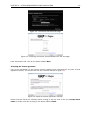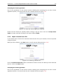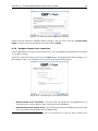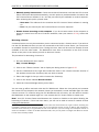
1
CLC Microbial Genomics Module
USER MANUAL
User manual for
CLC Microbial Genomics Module 1.0
Windows, Mac OS X and Linux
June 12, 2015
This software is for research purposes only.
CLC bio, a QIAGEN Company
Silkeborgvej 2
Prismet
DK-8000 Aarhus C
Denmark
Contents
1 Introduction to the CLC Microbial Genomics Module
1.1 The concept of the CLC Microbial Genomics Module
6
. . . . . . . . . . . . . . . .
6
1.2 Contact information . . . . . . . . . . . . . . . . . . . . . . . . . . . . . . . . . .
7
2 System requirements and installation
8
2.1 System Requirements . . . . . . . . . . . . . . . . . . . . . . . . . . . . . . . . .
8
2.2 Installation of modules . . . . . . . . . . . . . . . . . . . . . . . . . . . . . . . .
9
2.3 Workbench Licenses
. . . . . . . . . . . . . . . . . . . . . . . . . . . . . . . . .
9
2.3.1 Request an evaluation license . . . . . . . . . . . . . . . . . . . . . . . .
10
Direct download . . . . . . . . . . . . . . . . . . . . . . . . . . . . . . . .
11
Go to license download web page . . . . . . . . . . . . . . . . . . . . . .
11
Accepting the license agreement . . . . . . . . . . . . . . . . . . . . . . .
12
2.3.2 Download a license using a license order ID . . . . . . . . . . . . . . . . .
13
Direct download . . . . . . . . . . . . . . . . . . . . . . . . . . . . . . . .
13
Go to license download web page . . . . . . . . . . . . . . . . . . . . . .
13
Accepting the license agreement . . . . . . . . . . . . . . . . . . . . . . .
15
2.3.3 Import a license from a file . . . . . . . . . . . . . . . . . . . . . . . . . .
15
Accepting the license agreement . . . . . . . . . . . . . . . . . . . . . . .
15
2.3.4 Configure license server connection . . . . . . . . . . . . . . . . . . . . .
16
Borrowing a license . . . . . . . . . . . . . . . . . . . . . . . . . . . . . .
17
Common issues when using a network license
. . . . . . . . . . . . . . .
18
2.3.5 Download a static license on a non-networked machine . . . . . . . . . . .
19
2.4 Uninstall of modules
. . . . . . . . . . . . . . . . . . . . . . . . . . . . . . . . .
21
2.5 How to install a Server plugin . . . . . . . . . . . . . . . . . . . . . . . . . . . . .
21
2.5.1 Static license installation . . . . . . . . . . . . . . . . . . . . . . . . . . .
22
3
CONTENTS
4
2.5.2 Windows license download . . . . . . . . . . . . . . . . . . . . . . . . . .
23
2.5.3 Mac OS license download . . . . . . . . . . . . . . . . . . . . . . . . . . .
23
2.5.4 Linux license download . . . . . . . . . . . . . . . . . . . . . . . . . . . .
23
2.5.5 Download a static license on a non-networked machine . . . . . . . . . . .
23
2.5.6 Network license installation . . . . . . . . . . . . . . . . . . . . . . . . . .
25
2.5.7 Server plugin download, installation and removal . . . . . . . . . . . . . .
25
3 OTU clustering
27
3.1 Download OTU Reference Database . . . . . . . . . . . . . . . . . . . . . . . . .
27
3.2 Format Reference Database
. . . . . . . . . . . . . . . . . . . . . . . . . . . . .
27
3.3 Optional Merge Paired Reads . . . . . . . . . . . . . . . . . . . . . . . . . . . . .
28
3.4 Fixed Length Trimming . . . . . . . . . . . . . . . . . . . . . . . . . . . . . . . . .
29
3.5 Filter Samples Based on the Number of Reads . . . . . . . . . . . . . . . . . . .
30
3.6 OTUclustering . . . . . . . . . . . . . . . . . . . . . . . . . . . . . . . . . . . . .
30
3.6.1 OTUclustering parameters . . . . . . . . . . . . . . . . . . . . . . . . . . .
30
3.6.2 Add Metadata to OTU Abundance Table . . . . . . . . . . . . . . . . . . .
33
3.6.3 Remove OTUs with Low Abundance . . . . . . . . . . . . . . . . . . . . . .
33
3.6.4 Visualization of the OTU abundance table . . . . . . . . . . . . . . . . . .
34
4 Estimation of Alpha and Beta diversity
37
4.1 Align OTUs with MUSCLE . . . . . . . . . . . . . . . . . . . . . . . . . . . . . . .
37
4.2 Alpha Diversity . . . . . . . . . . . . . . . . . . . . . . . . . . . . . . . . . . . . .
38
4.2.1 Alpha diversity measures . . . . . . . . . . . . . . . . . . . . . . . . . . .
39
4.3 Beta Diversity . . . . . . . . . . . . . . . . . . . . . . . . . . . . . . . . . . . . .
40
4.3.1 Beta diversity measures . . . . . . . . . . . . . . . . . . . . . . . . . . . .
40
4.4 PERMANOVA Analysis . . . . . . . . . . . . . . . . . . . . . . . . . . . . . . . . .
41
4.5 Convert to Experiment . . . . . . . . . . . . . . . . . . . . . . . . . . . . . . . . .
42
4.6 Importing OTU abundance tables . . . . . . . . . . . . . . . . . . . . . . . . . . .
43
5 Workflows
44
5.1 Data QC and OTU clustering workflow . . . . . . . . . . . . . . . . . . . . . . . .
44
5.2 Estimate Alpha and Beta Diversities workflow . . . . . . . . . . . . . . . . . . . .
45
Bibliography
47
CONTENTS
Index
5
47
Chapter 1
Introduction to the CLC Microbial
Genomics Module
1.1
The concept of the CLC Microbial Genomics Module
The majority of microbial species present in the human body or indeed anywhere in the
environment have never been isolated, cultured or sequenced, due to our inability to reproduce
necessary growth conditions in the lab. Therefore, there are huge amounts of organismal
and functional novelty still to be discovered. Two central questions in microbial community
analysis ask: Which microbial species are present in a sample from a given habitat, and at
what frequencies? Microbiome analysis takes advantage of DNA molecular techniques and
sequencing technology in order to comprehensively retrieve specific regions of microbial genomic
DNA useful for taxonomical identification. For bacteria, the most widely used regions are parts
of the 16S rRNA gene. In a microbiome analysis workflow, total genomic DNA is extracted from
the sample(s) of interest, a region of the 16S gene is PCR amplified, and the resulting amplicon
is sequenced using an NGS machine. The bioinformatics task is then to assign taxonomy to
the reads and tally their occurrences. Due to the incomplete nature of bacterial taxonomy and
presence of sequencing errors in the NGS reads, a common approach is to cluster reads at
some level of similarity into pseudospecies called Operational Taxonomical Units (OTUs), where
all reads within e.g. 97% similarity are clustered together and represented by a single sequence.
PCR amplification can introduce artefacts in the form of chimeric sequences, where template
swapping results in a sequence having two or more parental templates. These chimeras can be
identified during the clustering step.
The features of the CLC Microbial Genomics Module 1.0 include:
• Trimming and merging of reads.
• Clustering of reads into OTUs.
• Generation of OTU tables.
• Working with metadata.
• Visualization options (stacked barplots, zoomable sunbursts).
• Multiple sequence alignment using MUSCLE.
6
CHAPTER 1. INTRODUCTION TO THE CLC MICROBIAL GENOMICS MODULE
7
• Phylogenetic tree construction using maximum likelihood.
• Estimation of alpha diversity.
• Rarefaction analysis.
• Estimation of beta diversity.
• Principal coordinates analysis
• PERMANOVA test
• Statistical tests for differential abundance
The primary output of the clustering and tallying process is an OTU table, listing the abundances
of OTUs in the samples under investigation, as well as new features allowing clear visualization
of the results. Secondary analyses include estimations of alpha and beta diversities, in addition
to statistical tests for differential abundance.
1.2
Contact information
The CLC Workbench is developed by:
CLC bio, a QIAGEN Company
Silkeborgvej 2
Prismet
8000 Aarhus C
Denmark
http://www.clcbio.com
VAT no.: DK 28 30 50 87
Telephone: 45 70 22 32 44
Fax: +45 86 20 12 22
E-mail: [email protected]
If you have questions or comments regarding the program, you can contact us through the support team as described here: http://www.clcsupport.com/clcgenomicsworkbench/
current/index.php?manual=Getting_help.html.
Chapter 2
System requirements and installation
2.1
System Requirements
To work with the CLC Microbial Genomics Module 1.0 you will need to have a CLC Genomics
Workbench version 8.0 or higher or the Biomedical Genomics Worbench 2.1 or higher installed
on your computer. With exception of the two editors below, the system requirements of CLC
Microbial Genomics Module 1.0 are the same as the ones required for the CLC Genomics
Workbench:
• Windows Vista, Windows 7, Windows 8 or Windows Server 2008.
• Mac OS X 10.7 or later.
• Linux: RHEL 5.0 or later. SUSE 10.2 or later. Fedora 6 or later.
• 2 GB RAM required.
• 4 GB RAM recommended.
• 1024 x 768 display required.
• 1600 x 1200 display recommended.
• Intel or AMD CPU required.
The PCoA 3D viewer requirements are the same as the 3D Molecule Viewer:
• System requirements
A graphics card capable of supporting OpenGL 2.0.
Updated graphics drivers. Please make sure the latest driver for the graphics card is
installed.
• System Recommendations
A discrete graphics card from either Nvidia or AMD/ATI. Modern integrated graphics
cards (such as the Intel HD Graphics series) may also be used, but these are usually
slower than the discrete cards.
8
CHAPTER 2. SYSTEM REQUIREMENTS AND INSTALLATION
9
A 64-bit workbench version.
The Sunburst viewer makes use of JavaFX and may not work on older Linux kernels. Un updated
list of requirements for JavaFX can be found at http://www.oracle.com/technetwork/
java/javafx/downloads/supportedconfigurations-1506746.html.
2.2
Installation of modules
Modules are installed using the Plugins and Resources Manager1 , which can be accessed via
the menu in the Workbench
Help | Plugins and Resources (
or via the Plugins (
)
) button on the Toolbar.
From within the Plugins and Resources Manager, choose the Download Plugins tab and click on
the CLC Workbench Client Plugin. Then click on the button labeled Download and Install.
If you are working on a system not connected to the internet, then you can also install the plugin
by downloading the cpa file from the plugins page of our website
http://www.clcbio.com/clc-plugin/
Then start up the Plugin manager within the Workbench, and click on the button at the bottom of
the Plugin manager labeled Install from File.
You need to restart the Workbench before the module is ready for use.
2.3
Workbench Licenses
When you have installed the CLC Microbial Genomics Module, and start it for the first time or
after installing a new major release, you will meet the license assistant, shown in figure 2.1.
To manually start up the License Manager for a Workbench plugin, first open the Plugin Manager
(see Section 2.2), select the relevant plugin or module, and press the button labeled Import a
new license.
To install a license, you must be running the program in administrative mode 2 .
The following options are available. They are described in detail in the sections that follow.
• Request an evaluation license. Request a fully functional, time-limited license (see below).
• Download a license. Use the license order ID received when you purchase the software to
download and install a license file.
• Import a license from a file. Import an existing license file, for example a file downloaded
from the web-based licensing system.
1
In order to install plugins on many systems, the Workbench must be run in administrator mode. On Windows Vista
and Windows 7, you can do this by right-clicking the program shortcut and choosing "Run as Administrator".
2
How to do this differs for different operating systems. To run the program in administrator mode on Windows
Vista, or 7, right-click the program shortcut and choose "Run as Administrator.
CHAPTER 2. SYSTEM REQUIREMENTS AND INSTALLATION
10
Figure 2.1: The license assistant showing you the options for getting started.
• Configure license server connection. If your organization has a CLC License Server, select
this option to configure the connection to it.
Select the appropriate option and click on button labeled Next.
To use the Download option in the License Manager, your machine must be able to access the
external network. If this is not the case, please see section 2.5.5.
2.3.1
Request an evaluation license
We offer a fully functional version of the CLC Microbial Genomics Module for evaluation purposes,
free of charge. Each user is entitled to 14 days demo of the CLC Microbial Genomics Module.
If you are unable to complete your assessment in the available time, please send an email to
[email protected] to request an additional evaluation period.
When you choose the option Request an evaluation license, you will see the dialog shown in
figure 2.2.
In this dialog, there are two options:
• Direct download. Download the license directly from CLC bio. This method requires that
the Workbench has access to the external network.
• Go to license download web page. In a browser window, show the license download web
page, which can be used to download a license file. This option is suitable in situations
where, for example, you are working behind a proxy, so that the Workbench does not have
direct access to the CLC Licenses Service.
CHAPTER 2. SYSTEM REQUIREMENTS AND INSTALLATION
11
Figure 2.2: Choosing between direct download or going to the license download web page.
If you select the option to download a license directly and it turns out that the Workbench does
not have direct access to the external network, (because of a firewall, proxy server etc.), you can
click Previous button to try the other method.
After selection on your method of choice, click on the button labeled Next.
Direct download
After choosing the Direct Download option and clicking on the button labeled Next, the dialog
shown in figure 2.3 appears.
Figure 2.3: A license has been downloaded.
A progress for getting the license is shown, and when the license is downloaded, you will be able
to click Next.
Go to license download web page
After choosing the Go to license download web page option and clicking on the button labeled
Next, the license download web page appears in a browser window, as shown in 2.4.
Click the Request Evaluation License button. You can then save the license on your system.
Back in the Workbench window, you will now see the dialog shown in 2.5.
Click the Choose License File button and browse to find the license file you saved. When you
CHAPTER 2. SYSTEM REQUIREMENTS AND INSTALLATION
12
Figure 2.4: The license download web page.
Figure 2.5: Importing the license file downloaded from the web page.
have selected the file, click on the button labeled Next.
Accepting the license agreement
Part of the installation of the license involves checking and accepting the end user license
agreement (EULA). You should now see the a window like that in figure 2.6.
Figure 2.6: Read the license agreement carefully.
Please read the EULA text carefully before clicking in the box next to the text I accept these
terms to accept, and then clicking on the button labeled Finish.
CHAPTER 2. SYSTEM REQUIREMENTS AND INSTALLATION
2.3.2
13
Download a license using a license order ID
Using a license order ID, you can download a license file via the Workbench or using an online
form. When you have chosen this option and clicked Next button, you will see the dialog shown
in 2.7. Enter your license order ID into the text field under the title License Order-ID. (The ID can
be pasted into the box after copying it and then using menus or key combinations like Ctrl+V on
some system or + V on Mac).
Figure 2.7: Enter a license order ID for the software.
In this dialog, there are two options:
• Direct download. Download the license directly from CLC bio. This method requires that
the Workbench has access to the external network.
• Go to license download web page. In a browser window, show the license download web
page, which can be used to download a license file. This option is suitable in situations
where, for example, you are working behind a proxy, so that the Workbench does not have
direct access to the CLC Licenses Service.
If you select the option to download a license directly and it turns out that the Workbench does
not have direct access to the external network, (because of a firewall, proxy server etc.), you can
click Previous button to try the other method.
After selection on your method of choice, click on the button labeled Next.
Direct download
After choosing the Direct Download option and clicking on the button labeled Next, the dialog
shown in figure 2.8 appears.
A progress for getting the license is shown, and when the license is downloaded, you will be able
to click Next.
Go to license download web page
After choosing the Go to license download web page option and clicking on the button labeled
Next, the license download web page appears in a browser window, as shown in 2.9.
CHAPTER 2. SYSTEM REQUIREMENTS AND INSTALLATION
14
Figure 2.8: A license has been downloaded.
Figure 2.9: The license download web page.
Click the Request Evaluation License button. You can then save the license on your system.
Back in the Workbench window, you will now see the dialog shown in 2.10.
Figure 2.10: Importing the license file downloaded from the web page.
Click the Choose License File button and browse to find the license file you saved. When you
have selected the file, click on the button labeled Next.
CHAPTER 2. SYSTEM REQUIREMENTS AND INSTALLATION
15
Accepting the license agreement
Part of the installation of the license involves checking and accepting the end user license
agreement (EULA). You should now see the a window like that in figure 2.11.
Figure 2.11: Read the license agreement carefully.
Please read the EULA text carefully before clicking in the box next to the text I accept these
terms to accept, and then clicking on the button labeled Finish.
2.3.3
Import a license from a file
If you already have a license file associated with the host ID of your machine,it can be imported
using this option.
When you have clicked on the Next button, you will see the dialog shown in 2.12.
Figure 2.12: Selecting a license file .
Click the Choose License File button and browse to find the license file. When you have selected
the file, click on the Next button.
Accepting the license agreement
Part of the installation of the license involves checking and accepting the end user license
agreement (EULA). You should now see the a window like that in figure 2.13.
CHAPTER 2. SYSTEM REQUIREMENTS AND INSTALLATION
16
Figure 2.13: Read the license agreement carefully.
Please read the EULA text carefully before clicking in the box next to the text I accept these
terms to accept, and then clicking on the button labeled Finish.
2.3.4
Configure license server connection
If your organization is running a CLC License Server, you can configure your Workbench to connect
to it to get a license.
To do this, select this option and click on the Next button. A dialog like that shown in figure 2.14
then appears. Here, you configure how to connect to the CLC License Server.
Figure 2.14: Connecting to a CLC License Server.
• Enable license server connection. This box must be checked for the Workbench is to
contact the CLC License Server to get a license for CLC Workbench.
• Automatically detect license server. By checking this option the Workbench will look for a
CLC License Server accessible from the Workbench3 .
3
Automatic server discovery sends UDP broadcasts from the Workbench on a fixed port, 6200. Available license
CHAPTER 2. SYSTEM REQUIREMENTS AND INSTALLATION
17
• Manually specify license server. If there are technical limitations such that the CLC License
Server cannot be detected automatically, use this option to provides details of machine the
CLC License Server software is on, and the port used by the software to receive requests.
After selecting this option, please enter:
Host name. The address for the machine the CLC Licenser Server software is running
on.
Port. The port used by the CLC License Server to receive requests.
• Disable license borrowing on this computer. If you do not want users of the computer to
borrow a license from the set of licenses available, then (see section 2.3.4), select this
option.
Borrowing a license
A network license can only be used when you are connected to the a license server. If you wish to
use the CLC Workbench when you are not connected to the CLC License Server, you can borrow
an available license for a period of time. During this time, there will be one less network license
available on the for other users. The Workbench must have a connection to the CLC License
Server at the point in time when you wish to borrow a license.
The procedure for borrowing a license is:
1. Go to the Workbench menu option:
Help | License Manager
2. Click on the "Borrow License" tab to display the dialog shown in figure 2.15.
3. Use the checkboxes at the right hand sideof the table in the License overview section of
the window to select the license(s) that you wish to borrow.
4. Select the length of time you wish to borrow the license(s).
5. Click on the button labeled Borrow Licenses.
6. Close the License Manager when you are done.
You can now go offline and work with the CLC Workbench. When the time period you borrowed
the license for has elapsed, the network license you borrowed is made available again for other
users to access. To continue using the CLC Workbench with a license, you will need to connect
the Workbench to the network again so it can contact the CLC Licene Server to obtain one.
Note! Your CLC License Server administrator can choose to disable to the option allowing the
borrowing of licenses. If this has been done, you will not be able to borrow a network license
using your Workbench.
servers respond to the broadcast. The Workbench then uses TCP communication for to get a license, assuming one
is available. Automatic server discovery works only on local networks and will not work on WAN or VPN connections.
Automatic server discovery is not guaranteed to work on all networks. If you are working on an enterprise network on
where local firewalls or routers cut off UDP broadcast traffic, then you may need to configure the details of the CLC
License server manually instead.
CHAPTER 2. SYSTEM REQUIREMENTS AND INSTALLATION
18
Figure 2.15: Borrow a license.
Common issues when using a network license
No license available at the moment If all the network licenses or CLC Workbenchare in use,
you will see a dialog like that shown in figure 2.16 when you start up the Workbench.
Figure 2.16: This window appears when there are no available network licenses for the software
you are running.
This means others are using the network licenses. You will need to wait for them to return their
licenses before you can continue to work with a fully functional copy of software. If this is a
frequent issue, you may wish to discuss this with your CLC License Server administrator.
Clicking on the Limited Mode button in the dialog allows you to start the Workbench with
functionality equivalent to the CLC Sequence Viewer. This includes the ability to access your CLC
data.
CHAPTER 2. SYSTEM REQUIREMENTS AND INSTALLATION
19
Lost connection to the CLC License Server If the Workbench connection to the CLC License
Server is lost, you will see a dialog as shown in figure 2.17.
Figure 2.17: This message appears if the Workbench is unable to establish a connection to a CLC
License server.
If you have chosen the option to Automatically detect license server and you have not succeeded
in connecting to the License Server before, please check with your local IT support that automatic
detection will be possible to do at your site. If it is not possible at your site, you will need to
manually configure the CLC License Server settings using the License Manager, as described
earlier in this section.
If you have successfully contacted the CLC License Server from your Workbench previously,
please consider discussing this issue with your CLC License Server administrator or your local
IT support, to make sure that the CLC License Server is running and that your Workbench can
connect to it.
There may be situations where you wish to use a different license or view
information about the license(s) the Workbench is currently using. To do this, open the License
Manager using the menu option:
Help | License Manager (
)
The license manager is shown in figure 2.18.
This dialog can be used to:
• See information about the license (e.g. what kind of license, when it expires)
• Configure how to connect to a license server (Configure License Server the button at the
lower left corner). Clicking this button will display a dialog similar to figure 2.14.
• Upgrade from an evaluation license by clicking the Upgrade license button. This will display
the dialog shown in figure 2.1.
• Export license information to a text file.
• Borrow a license
If you wish to switch away from using a network license, click on the button to Configure License
Server and uncheck the box beside the text Enable license server connection in the dialog.
When you restart the Workbench, you can set up the new license as described in section 2.3.
2.3.5
Download a static license on a non-networked machine
To download a static license for a machine that does not have direct access to the external
network, you can follow the steps below:
CHAPTER 2. SYSTEM REQUIREMENTS AND INSTALLATION
20
Figure 2.18: The license manager.
• Install the CLC Microbial Genomics Module on the machine you wish to run the software
on.
• Start up the software as an administrative user and find the host ID of the machine that
you will run the CLC Workbench on. You can see the host ID the machine reported at the
bottom of the License Manager window in grey text.
• Make a copy of this host ID such that you can use it on a machine that has internet access.
• Go to a computer with internet access, open a browser window and go to the relevant
network license download web page:
• For Workbenches released from January 2013 and later, (e.g. the Genomics Workbench
version 6.0 or higher, and the Main Workbench, version 6.8 or higher), please go to:
https://secure.clcbio.com/LmxWSv3/GetLicenseFile
• Paste in your license order ID and the host ID that you noted down in the relevant boxes on
the webpage.
• Click 'download license' and save the resulting .lic file.
• Open the Workbench on your non-networked machine. In the Workbench license manager
choose 'Import a license from a file'. In the resulting dialog click 'choose license file' to
browse the location of the .lic file you have just downloaded.
If the License Manager does not start up by default, you can start it up by going to the Help
menu and choosing License Manager.
• Click on the Next button and go through the remaining steps of the license manager wizard.
CHAPTER 2. SYSTEM REQUIREMENTS AND INSTALLATION
2.4
21
Uninstall of modules
Modules are uninstalled using the plugin manager:
Help in the Menu Bar | Plugins and Resources... (
or Plugins (
)
) in the Toolbar
This will open the dialog shown in figure 2.19.
Figure 2.19: The plugin manager with plugins installed.
The installed plugins and modules are shown in this dialog. To uninstall:
Click the CLC Microbial Genomics Module | Uninstall
If you do not wish to completely uninstall the module but you don't want it to be used next time
you start the Workbench, click the Disable button.
When you close the dialog, you will be asked whether you wish to restart the workbench. The
module will not be uninstalled until the workbench is restarted.
2.5
How to install a Server plugin
If you wish to use the tools and functionalities of the CLC Microbial Genomics Module with a CLC
Genomics Server, you must purchase a Microbial Genomics Extension license and install it on
your CLC Server as explained in the following steps:
1. Install plugin licenses to each machine with the CLC Server software installed, as described
below.
2. Install the Server plugin on only the master CLC Server in the server setup, as described in
section 2.5.7.
CHAPTER 2. SYSTEM REQUIREMENTS AND INSTALLATION
22
3. Restart all CLC Servers in the setup. How to stop and start CLC Servers is covered
in the CLC Server manual at http://www.clcsupport.com/clcgenomicsserver/
current/admin/index.php?manual=Starting_stopping_server.html.
There are three different server setups. A short description of each setup and a summary of the
plugin licensing requirements are below.
• Single server setup - A single machine is running the CLC Server software. Jobs are
submitted to this server, which receives and executes them. In this setup, a single machine
acts both as a master and an executor of jobs. Here, a single static license for the plugin
is installed in the CLC Server software.
• Job node setup - More than one machine is running the CLC Server software. The system
acting as the master server receives job requests and then submits these jobs to other
machines, the job nodes, for execution. Here, a single static license is installed on each
machine running the CLC Server software. That is, a static license is installed on the
master node and on each job node.
• Grid setup - One machine runs the CLC Server software and receives job requests. It then
submits these to a third party scheduler. The scheduler then chooses an appropriate grid
machine, or node, to submit a given job to for execution. Here, a a single static license
for the plugin is installed on the master server, and the same number of network plugin
licenses as there are network gridworker licenses needs to be made available by installing
these in the CLC License Server software.
For a more detailed description of the different server setups, please refer to the CLC Server manual at: http://clcsupport.com/clcgenomicsserver/current/admin/index.php?
manual=Job_Distribution.html
2.5.1
Static license installation
In each of the server models described above, a static license is installed in the CLC Server on
a master machine. In the case of a job node setup, static licenses are also installed on each
machine acting as a job node.
Static licenses for the Server CLC Workbench are downloaded and installed into the licenses
folder in the CLC Server installation area. Downloading a license is similar for all supported
platforms, but varies in certain details. Please see the platform-specific instructions below for
details on how to download a license file on the system you are running the CLC Server on. See
section 2.5.5 for a description on how to download a license for a machine that does not have
access to the internet.
For the master machine and for each machine in a job node setup:
1. Log on to the machine that is running the CLC Server.
2. Move into the CLC Server installation directory, where the license download script can be
found.
3. Download and install the CLC Workbench license as described in the relevant section
below.
CHAPTER 2. SYSTEM REQUIREMENTS AND INSTALLATION
2.5.2
23
Windows license download
License files are downloaded using the licensedownload.bat script. To run the script,
right-click on the file and choose Run as administrator. This will present a window as shown in
figure 2.20.
Figure 2.20: Download a license based on the Order ID.
Paste the Order ID supplied by CLC bio (right-click to Paste) and press Enter. Please contact
[email protected] if you have not received an Order ID.
Note that if you are upgrading an existing license file, this needs to be deleted from the
licenses folder. When you run the downloadlicense.command script, it will create a new
license file.
2.5.3
Mac OS license download
License files are downloaded using the downloadlicense.command script. To run the script,
double-click on the file. This will present a window as shown in figure 2.21.
Paste the Order ID supplied by CLC bio and press Enter. Please contact [email protected] if
you have not received an Order ID.
Note that if you are upgrading an existing license file, this needs to be deleted from the
licenses folder. When you run the downloadlicense.command script, it will create a new
license file.
2.5.4
Linux license download
License files are downloaded using the downloadlicense script. Run the script and paste the
Order ID supplied by CLC bio. Please contact [email protected] if you have not received an
Order ID.
Note that if you are upgrading an existing license file, this needs to be deleted from the
licenses folder. When you run the downloadlicense script, it will create a new license file.
2.5.5
Download a static license on a non-networked machine
To download a static license for a machine that does not have direct access to the external
network, you can follow the steps below after the Server software has been installed.
CHAPTER 2. SYSTEM REQUIREMENTS AND INSTALLATION
24
Figure 2.21: Download a license based on the Order ID.
• Determine the host ID of the machine the server will be running on by running the same
tool that would allow you to download a static license on a networked machine. The name
of this tool depends on the system you are working on:
Linux: downloadlicense
Mac: downloadlicense.command
Windows: licensedownload.bat
When you run the license download tool, the host ID for the machine you are working on
will be printed to the terminal.
• Make a copy of this host ID such that you can use it on a machine that has internet access.
• Go to a computer with internet access, open a browser window and go to the relevant
network license download web page:
https://secure.clcbio.com/LmxWSv3/GetLicenseFile
• Paste in your license order ID and the host ID that you noted down earlier into the relevant
boxes on the webpage.
• Click on 'download license' and save the resulting .lic file.
• Take this file to the machine with the host ID that you used when downloading the license
file. Place it in the folder called 'licenses' that can be found within the CLC Server
installation directory.
• Restart the CLC Server software.
CHAPTER 2. SYSTEM REQUIREMENTS AND INSTALLATION
2.5.6
25
Network license installation
Network licenses are necessary to run CLC Microbial Genomics Module analysis tasks on grid
nodes. Network licenses are made available using a separate piece of software called the
CLC License Server. This software is normally run as a service. CLC client software, such as
Workbenches and gridworkers, contact the CLC License Server to obtain a network license when
needed. For a description of how to download and install a license on a CLC License Server,
please refer to the following section in the CLC License Server manual: http://clcsupport.
com/clclicenseserver/current/index.php?manual=License_download.html
The same number of network plugin licenses as there are CLC gridworker licenses for the CLC
Server setup are required. A license order ID is used when downloading a single license file.
This license file includes information about how many network licenses are associated with the
license order ID.
2.5.7
Server plugin download, installation and removal
1. Download the CLC Workbench plugin for the CLC Server as a .cpa file from http:
//www.clcbio.com/clc-plugin/#Server.
2. Install the plugin .cpa file on the master CLC Server using the Server web administrative
interface. The plugin should only be installed on the master server in all server setup
models. It does not need to be manually installed on any machine acting as an execution
node.
To install the plugin:
(a) Go to the Plugins section under the Admin (
) tab (see figure 2.22).
(b) Click on the Browse button and locate the .cpa file for the plugin to install.
Logging into the web administrative interface is described in the CLC Server manual at:
http://www.clcsupport.com/clcgenomicsserver/current/admin/index.php?
manual=Logging_into_administrative_interface.html.
3. Restart the master CLC Server.
Starting, stopping and restarting the CLC Server software is described in the CLC Server
manual started at:
http://www.clcsupport.com/clcgenomicsserver/current/admin/index.php?
manual=Starting_stopping_server.html
4. For job node setups only:
(a) Wait until the master CLC Server is up and running normally. Then restart each job
node CLC Server so that the plugin is ready to run on each node.
(b) In the web administrative interface on the master CLC Server, check that the plugin is
enabled for each job node. This is described in more detail in the CLC Server manual
at:
http://www.clcsupport.com/clcgenomicsserver/current/admin/index.
php?manual=Configuring_your_setup.html
CHAPTER 2. SYSTEM REQUIREMENTS AND INSTALLATION
26
Figure 2.22: Installing and uninstalling CLC Server plugins is done via the Plugins section of the
web administrative interface.
To uninstall a CLC Server plugin, simply click on the button that has Uninstall on its label next to
the relevant plugin.
Chapter 3
OTU clustering
3.1
Download OTU Reference Database
OTU reference databases contain representative OTU sequences and their taxonomy. They are
needed to perform reference-based OTU clustering. Three popular reference OTU databases,
clustered at various similarity percentages, can be downloaded using the Download OTU
Reference Database tool:
• Greengenes: 16S rRNA gene from ribosomal Small Subunit for Prokaryotic taxonomic assignment clustered OTUs at different percentages. http://greengenes.secondgenome.
com/downloads
• Silva/Arb SSU: 16S/18S rRNA from ribosomal Small Subunit for Prokaryotic and Eukaryotic
taxonomic assignment clustered OTUs at different percentages. http://www.arbsilva.de/download/archive/qiime/
• UNITE: ITS spacer clustered OTUs at different percentages for fungal taxonomic assignment.
https://unite.ut.ee/repository.php
To run the tool, go to Toolbox | OTUclustering ( ) | Download OTU Reference Database ( ),
select the database needed and specify where to save it. When using this tool, the databases
downloaded are automatically formatted. If you wish to format your own database, use the tool
called Format Reference Database.
3.2
Format Reference Database
In addition to the download of reference databases using the Download OTU Reference Database
tool, you can format your own databases by running the Format Reference Database tool:
Toolbox | OTUclustering (
) | Format Reference Database (
).
This tool takes as input QIIME-format fasta files (typically clustered into OTUs at 99, 97, 94,
and 90 percent similarity) and corresponding taxonomy mapping files. Each line of the taxonomy
file should contain an OTU name and its taxonomy, where taxonomy levels are separated with
semicolons. For example, the following line
o123
k__Bacteria;p__Bacteroidetes;c__Sphingobacteria;o__;f__;g__;s__.
27
CHAPTER 3. OTU CLUSTERING
28
indicates that the OTU o123 belongs to the class Sphingobacteria and that its taxonomy is
specified only up to the class level.
3.3
Optional Merge Paired Reads
In order to use the highest quality sequences for clustering, it is recommended to merge paired
read data. If the read length is smaller than the amplicon size, forward and reverse reads are
expected to overlap in most of their 3' regions. Therefore, one can merge the forward and reverse
reads to yield one high quality representative using the Optional Merge Paired Reads tool. The
Optional Merge Paired Reads tool will merge paired-end reads according to some pre-selected
merge parameters: the overlap region and the quality of the sequences. For example, for a
designed 150 bp overlap, a maximum score of 150 is achievable, but as the real length of the
overlap is unknown, a lower minimum score should be chosen. Also, some mismatches and
InDels should be allowed, especially if the sequence quality is not perfect. You can also set
penalties for mismatch, gap and unaligned ends.
To run the Optional Merge Paired Reads tool, go to Toolbox | OTUclustering (
Merge Paired Reads ( ).
) | Optional
Select any number of sequences as input. The tool accepts both paired and unpaired reads but
will only merge the paired reads while returning the unpaired ones as "not merged" reads in
the output. Note that paired reads have to be in forward-reverse orientation. After merging, the
merged reads will always be in the forward orientation.
Click Next to open the dialog shown in figure 3.1.
Figure 3.1: Alignment parameters.
In order to understand how these parameters should be set, an explanation of the merging
algorithm is needed: Because the fragment size is not an exact number of base pairs and is
different from fragment to fragment, an alignment of the two reads has to be performed. If the
alignment is good and long enough, the reads will be merged. Good enough in this context means
that the alignment has to satisfy some user-specified score criteria (details below). Because of
sequencing errors that typically are more abundant towards the end of the read, the alignment is
not expected always to be perfect, and the user can decide how many errors are acceptable. Long
enough in this context means that the overlap between the reads has to be non-coincidental.
Merging two reads that do not really overlap, leads to errors in the downstream analysis, thus it
is very important to make sure that the overlap is big enough. If only a few bases overlap was
required, some read pairs will match by chance, so this has to be avoided.
The following parameters are used to define what is good enough and long enough.
CHAPTER 3. OTU CLUSTERING
29
• Mismatch cost: The alignment awards one point for a match, and the mismatch cost is set
by this parameter. The default value is 2.
• Minimum score: This is the minimum score of an alignment to be accepted for merging.
The default value is 8. As an example: with default settings, this means that an overlap of
11 bases with one mismatch will be accepted (10 matches minus 2 for a mismatch).
• Gap cost: This is the cost for introducing an insertion or deletion in the alignment. The
default value is 3.
• Maximum unaligned end mismatches: The alignment is local, which means that a number
of bases can be left unaligned. If the quality of the reads is dropping to be very poor
towards the end of the read, and the expected overlap is long enough, it makes sense
to allow some unaligned bases at the end. However, this should be used with great care
which is why the default value is 0. As explained above, a wrong decision to merge the
reads leads to errors in the downstream analysis, so it is better to be conservative and
accept fewer merged reads in the result. Please note that even with the alignment scores
above the minimum score specified in the tool setup, the paired reads also need to have
the number of end mismatches below the "Maximum unaligned end mismatches" value
specified in the tool setup to be qualified for merging.
The main result will be two sequence lists for each sample selected as input to the tool: one
containing the merged reads (labeled as "merged"), and one containing the reads that could not
be merged (labeled as "not merged"). Note that low quality can be one of the reasons why a pair
cannot be merged. Hence, the list of reads that could not be paired is more likely to contain
more reads with errors than the one with the merged reads.
3.4
Fixed Length Trimming
In order to compare sequences and cluster them, they all need to be of exact same length. All
reads which are shorter than the cut-off are discarded, and reads longer than that are trimmed
back to the chosen length.
To run the tool, go to Toolbox | OTUclustering (
sequences you would like to trim.
) | Fixed Length Trimming (
) and select the
In the next wizard window you can enter manually the desired length for the trimmed reads.
Alternatively, the Fixed length Trimming algorithm can calculate the trimming cut-off value as the
mean length of the merged reads minus one standard deviation. If this option is chosen, it is
important that all samples are trimmed at the same time as the mean and standard deviation
for the combined reads in all samples needs to be estimated at once.
You can also offset one adapter or barcode by typing the nucleotide sequence in the Primer
offset window. Exact matching is performed but ambiguous symbols are allowed. For more
than one adapter, we recommend to perform prior to the Fixed Length trimming a Trim Sequences step from the NGS Core Tools in which you can import an adapter list (see the CLC
Microbial Genomics Module tutorial, or the Adapter Trimming section of the CLC Genomics
Workbench manual (http://www.clcsupport.com/clcgenomicsworkbench/current/
index.php?manual=Adapter_trimming.html).
CHAPTER 3. OTU CLUSTERING
3.5
30
Filter Samples Based on the Number of Reads
In order to cluster accurately samples, they should have comparable coverage. Sometimes,
however, DNA extraction, PCR amplification, library construction or sequencing has not been
entirely successful, and a fraction of the resulting sequencing data will be represented by too few
reads. These samples should be excluded from further analysis using the Filter Samples Based
on the Number of Reads tool.
To run the tool, go to Toolbox | OTUclustering (
Reads ( ).
) | Filter Samples Based on the Number of
The tool requires that the input reads from each sample must be either all paired or all single.
This check ensures that the samples are comparable, as the number of reads before merging
paired reads is twice as great as the number of merged reads. The preferred way to run this
tool with OTU sequencing data is to use merged reads obtained from the Optional Merge Paired
Reads tool.
The threshold for determining whether a sample has sufficient coverage is specified by the
parameters minimum number of reads and minimum percent from the median. The algorithm
filters out all samples whose number of reads is less than the minimum number of reads or
less than the minimum percent from the median times the median number of reads across all
samples.
The primary output is a table describing how many reads are in a particular sample and if they
passed or failed the quality control (see figure 3.2).
Figure 3.2: Output table from the Filter Samples Based on the Number of Reads tool.
In the next wizard window you can decide to Copy samples with sufficient coverage as well as to
Copy the discarded samples. Copying the samples with sufficient coverage will give you a new
list of sequences that you can use in your following analyses because it does not contain the
reads of poor quality that failed the Remove the samples with Low Coverage analysis.
3.6
OTUclustering
The OTUclustering tool clusters a collection of fixed length trimmed reads to operational taxonomy
units.
To run the tool, go to Toolbox | OTUclustering (
3.6.1
) | OTUclustering (
).
OTUclustering parameters
After having selected the sequences you would like to cluster, the wizard offers to set some
general parameters (see figure 3.3).
CHAPTER 3. OTU CLUSTERING
31
Figure 3.3: Outputtable from the Remove Low Coverage Samples tool.
You can choose to perform a De novo OTU clustering, or you can perform a Reference based
OTU clustering. The following parameters can then be set:
• OTU database Specify here the reference database to be used for Reference based OTU
clustering. Reference databases can be created by the Download OTU Reference Database
or the Format Reference Database tools.
• Use the similarity percent specified by the reference database Allows to use the same
similarity percent value (see below) that was used when creating the reference database.
This parameter is available only when performing a reference based OTU clustering.
Selecting this parameter will disable the similarity percent parameter.
• Allow creation of new OTUs Allows sequences which are not already represented at
the given similarity distance in the database to form a new cluster, and a new centroid is
chosen. This parameter can be set only when performing a Reference based OTU clustering.
Disallowing the creation of new OTUs is also known as closed reference OTU picking.
• Taxonomy similarity percentage Specifies the similarity percentage to be used when
annotating new OTUs. This parameter is available only when Allow creation of new OTUs
is selected.
• Similarity percentage: Specifies the required percentage of identity between a read and
the centroid of an OTU for the read to join the OTU cluster.
• Minimum occurrences: Specifies the minimum number of duplicates for specific read-data
before it will be included in further analyses. For instance, if set to 2, at least two reads
with the same exact nucleotides needs to exist in the input for the data to propagate to
further analysis. Other data will be thrown away. This can for instance be used to filter out
singletons. Note that matches does not need to be exact when the Fuzzy match duplicates
option is used.
CHAPTER 3. OTU CLUSTERING
32
• Fuzzy match duplicates: Specifies how duplicates are defined. If the option is not selected
two reads are only duplicates if they are exactly equal. If the option is selected, two reads
are duplicates if they are almost equal, i.e. all differences are SNVs and there are not too
many of them (≤ 2%). This pseudo-merging is done by lexicographically sorting the input
and looking in the neighborhood of the read being processed. The reads are processed
from most abundant (in a completely equivalent sense) to the least. In this way two
singletons can for instance be pseudo-merged together and be included for further study
despite the Minimum occurrences option having specified 2. Upon further analysis a group
can be split into several OTUs if not all members are within the specified threshold from
the ``OTU-leader''.
• Find best match: If the option is not selected, the read becomes a member of the first
OTU-database entry found within the specified threshold. If the option is selected all
database entries are tested and the read becomes a member of the best matching result.
Note that ``first'' and ``all'' are relative terms in this case as kmer-searches are used to
speed up the process. ``All'' only includes the database entries that the kmer search deems
close enough, i.e., database entries that cannot be within the specified threshold will be
filtered out at this step. ``First'' is the first matching entry as returned by the kmer-search
which will sort by the number of kmer-matches.
• Detect chimeras: Chimeric sequences are frequent artifacts of PCR reactions. They are
detected by assessing whether a sequence is likely to have two different and more frequent
"parent" sequences in the current collection of OTUs, meaning that two fragments of the
sequence map to different sequences.
• Chimera crossover cost: The cost of doing a chimeric crossover, i.e. the higher the cost
the less likely it is that a read is marked as chimeric.
• Chimera crossover cost is percent: Whether the above cost is an absolute value or a
percentage value (i.e. an absolute value will be automatically calculated based on the read
length).
• Kmer size: The size of the kmer to use in regards to the kmer usage in finding the best
match.
Chimera detection is performed by kmer searches as follows:
• All database entries and the read being processed are split into 4 equally sized portions
with an additional 3 half-way-shifted to cover the merge-points. This results in 7 different
kmer-search-options. Each of these is queried for matches within some threshold, and only
the results are processed further. A database entry has to fit well in at least one of these
7 portions for the database-entry to be relevant.
• Given the 7 sets of database entries some entries may just be present in one of the sets.
For these entries, some may be duplicates in the region they represent. The duplicates are
filtered out and only an arbitrary representative of the duplicates is kept.
The OTU clustering tool produces several outputs: a sequence list of the OTU centroids and/or
of the Chimeras, and abundance tables with the newly created OTUs and/or the chimeras. Each
table give abundance of the OTU or chimeras at each site, as well as the total abundance for all
samples.
CHAPTER 3. OTU CLUSTERING
3.6.2
33
Add Metadata to OTU Abundance Table
In order to enhance the visualization functionality of the OTU abundance table, it is useful to
decorate it with metadata on the samples. To run the tool go to: Toolbox | OTUclustering ( ) |
Add Metadata to OTU Abundance Table ( )
Choose an OTU table as input. In the next wizard window you can select a file describing the
metadata on your local computer (figure 3.4).
Figure 3.4: Setting up metadata parameters.
The metadata should be formatted in a tabular file format (.xls, .xlsx, .csv). The first row of
the table should contain column headers. There should be one column called ``Name'' and the
entries in this column should match the names of the reads selected for OTUclustering. This
column is used to match row in the table with samples present in the OTU table, so if the
names do not match you will not be able to aggregate your data at all. There can be as many
other columns as needed, and these information can be used as grouping variables to improve
visualization of the results or to perform additional statistical analyses. If you wish to ignore a
column without deleting it from your file, simply delete the text in the header row.
3.6.3
Remove OTUs with Low Abundance
Low abundance OTUs can eliminated from the OTU table if they have fewer than a given count
across all the samples in the experiment.
To run the tool, go to Toolbox | OTUclustering (
) | Remove OTUs with Low Abundance (
).
Choose an OTU table as input, select the filtering parameters and save the table. The threshold
for determining whether an OTU has sufficient abundance is specified by the parameters minimum
combined abundance and minimum combined abundance (% of all the reads). The algorithm
filters out all OTUs whose combined abundance across all samples is less than the minimum
combined abundance or whose combined abundance is less than the minimum combined
abundance (% of all the reads) across all samples. The default value for the Minimum combined
abundance is set at 10.
CHAPTER 3. OTU CLUSTERING
3.6.4
34
Visualization of the OTU abundance table
The OTU clustering tool produces several outputs: a sequence list of the OTU centroids or of the
Chimeras, and abundance tables with the newly created OTUs or the chimeras. Each table give
abundance of the OTU or chimeras at each site as well as the total abundance for all samples.
There are a number of ways of visualizing the contents of an OTU abundance table:
• Table view (
) The table display the following columns:
Name The name of the OTU, specified by either the reference database or by the OTU
representative.
Taxonomy The taxonomy of the OTU, as specified by the reference database when a
database entry was used as Reference.
Combined Abundance The total number of reads belonging to the OTU across all
samples.
Min Minimum abundance across all samples
Max Maximum abundance across all samples
Mean Mean abundance of all samples
Median Median abundance of all samples
Std Standard deviation of all samples
Abundance for each sample The number of reads belonging to the OTU in a specific
sample.
Sequence The sequence of the centroid of the OTU.
Under the tab Data in the right side panel, you can switch between absolute counts and
relative abundances. You can also combine absolute counts and relative abundances by
taxonomic levels by selecting the appropriate phylum in the Aggregate taxonomy drop-down
menu. Finally, if you have previously annotated your table with Metadata (see section 3.6.2),
you can Aggregate sample by the groups previously defined in your metadata table. This is
useful when analyzing replicates from the same sample origin.
• Stacked Bar Chart and Stacked Area Chart ( ) In the Stacked Bar (figure 3.5) and
Stacked Area Charts (figure 3.6), the metadata can be used to aggregate groups of
columns (samples) by selecting the relevant metadata category in the right hand side
panel. Also, the data can be aggregated at any taxonomy level selected. The relevant data
points will automatically be summed accordingly.
Holding the pointer over a colored area in any of the plots will result in the display of the
corresponding taxonomy label and counts. The slider Filter level allows the setting of a
viewing filter on the minimum counts for individual viewing instead of being aggregated in
the "Other" category displayed in the top field of the chart. One can select which taxonomy
level to color, and change the default colors manually. Colors can be be specified at the
same taxonomy level as the one use to aggregate the data or at a lower level. When
lower taxonomy levels are chosen in the data aggregation field, the color will be inherited
in alternating shadings. Using the bottom right-most button (Save/restore settings ( )),
the settings can be saved and applied in other plots, allowing visual comparisons across
analyses.
CHAPTER 3. OTU CLUSTERING
35
Figure 3.5: Stacked bar of the microbial community at the order level for 3 different sites.
Figure 3.6: Stacked area of the microbial community at the phylum level for 12 different sites.
• Zoomable Sunbursts ( ) The Zoomable Sunburst viewer lets the user select how many
taxonomy level counts to display, and which level to color. Lower levels will inherit the color
in alternating shadings. Taxonomy and relative abundances are displayed in a legend to the
left of the plot when hovering over the sunburst viewer with the mouse. The metadata can
be used to select which sample or group of samples to show in the sunburst (figure 3.7).
Clicking on a lower level field will render that field the center of the plot and display lower
level counts in a radial view. Clicking on the center field will render the level above the
current view the center of the view (figure 3.8).
CHAPTER 3. OTU CLUSTERING
36
Figure 3.7: Sunburst view of the microbial community showing all taxa belonging to the kingdom
bacteria.
Figure 3.8: Sunburst view of the microbial community zoomed to show all taxa belonging to the
phylum bacteroidetes.
Chapter 4
Estimation of Alpha and Beta diversity
Two levels of diversity are typically considered in microbial ecology: alpha- and beta-diversity.
Alpha-diversity estimates describe the number of species (or similar metrics) in a single sample,
whereas beta-diversity compares the number of species (or similar metrics) across samples
[Whittaker, 1972].
Some measures of estimate alpha and beta diversity require a phylogenetic tree of all OTUs.
The phylogenetic tree is reconstructed based on a multiple sequence alignment (MSA) of the
OTU sequences. Therefore, as a pre-requisite, a MSA needs to be created and a phylogeny
reconstructed.
4.1
Align OTUs with MUSCLE
In order to estimate Alpha and Beta diversity, you must use first use the Align OTUs with MUSCLE
tool of the CLC Microbial Genomics Module:
Toolbox | OTUclustering (
) | Align OTUs using MUSCLE (
).
Choose an OTU abundance table as input. the next wizard window allows you to set up the
alignment parameters with MUSCLE (figure 4.1).
Figure 4.1: Set up parameters for aligning sequences with MUSCLE.
37
CHAPTER 4. ESTIMATION OF ALPHA AND BETA DIVERSITY
38
• Find Diagonals: you can decide on some restrictive parameters for your analysis: the
Maximum Hours the analysis should last, the Maximum Memory in mb that should be
used for the analysis, or the Maximum Iterations the analysis should make. The latter is
set to 16 by default.
• Filtering Parameters: The algorithm filters out all OTUs whose combined abundance across
all samples is less than the minimum combined abundance or whose combined abundance
is less than the minimum combined abundance (% of all the reads) across all samples.
The default value for the Minimum combined abundance is set at 10. Moreover, you can
specify the Maximum number of sequences to be aligned, so that only the sequences
with the highest combined abundances will be used. Note that reducing the number of
sequences will speed up the alignment and the construction of phylogeny trees.
Note that by default only the top 100 most abundant OTUs are aligned using MUSCLE and
used to reconstruct the phylogeny tree in the next step. This phylogenetic tree is used for
calculating the phylogenetic diversity and the UniFrac distances, so these measures disregard
the low abundance OTUs by default. If more OTUs are to be included, the default settings for the
MUSCLE alignment need to be changed accordingly.
For further analysis with the Alpha and Beta diversity tools, save the alignment and construct a
phylogeny using the Maximum Likelihood Phylogeny tool from CLC Workbench core tools in Toolbox
| Classical Sequence Analysis ( ) | Alignments and Trees ( ) | Maximum Likelihood Phylogeny
( ). Users of the Biomedical Genomics Worbench will find the tool under Toolbox | OTUclustering
( ). For more information, see http://www.clcsupport.com/clcgenomicsworkbench/
current/index.php?manual=Maximum_Likelihood_Phylogeny.html.
4.2
Alpha Diversity
Alpha diversity is the diversity within a particular area or ecosystem; usually expressed by the
number of species (i.e., species richness) in that ecosystem. Alpha diversity estimates are
dependent on sampling depth, and hence rarefaction analysis is integral to this analysis step.
To run the tool go to Toolbox | OTUclustering ( ) | Alpha Diversity ( ). Choose an OTU
table to use as input. The next wizard window offers you to set up different analysis parameters
(figure 4.2). For example, you can select which diversity measures to calculate (see section 4.2.1),
specify the appropriate phylogenetic tree for computing phylogenetic diversity, and parameterize
the rarefaction analysis.
The rarefaction analysis is done by sub-sampling the OTU abundances in the different samples
at different depths. The range of depths to be sampled is defined by the parameters Minimum
depth to sample and Maximum depth to sample. If the maximum depth is set to 0, the number
of reads of the most abundant sample is used. The number of different depths to be sampled is
specified by the Numbers of depths to be sampled parameters. For example, if you choose to
sample 5 depths between 1000 and 5000, the algorithm will sub-sample each sample at 1000,
2000, 3000, 4000, and 5000 reads. At each depth, the algorithm subsamples the data several
times, according to the Replicates at each depth. You can choose whether the sampling should
be performed with or without replacement by setting the Sample with replacement parameter.
CHAPTER 4. ESTIMATION OF ALPHA AND BETA DIVERSITY
39
Figure 4.2: Set up parameters for the Alpha Diversity tool.
4.2.1
Alpha diversity measures
The available diversity measures are:
• Number of OTUs: The number of OTUs observed in the sample.
• Chao 1 bias-corrected: Chao1-bc = D +
• Chao 1: Chao1 = D +
f12
2f2 .
• Simpson's index: SI = 1 −
n
P
i=1
• Shannon entropy: H =
f1 (f1 −1)
2(f2 +1) .
n
P
p2i .
pi log2 pi .
i=1
where n is the number of OTUs; D is the number of distinct OTUs observed in the sample; f1
is the number of OTUs for which only one read has been found in the sample; f2 is the number
of OTUs for which two reads have been found in the sample; and pi is the fraction of reads that
belong to OTU i.
If a phylogenetic tree is provided as input, the following distance is also available:
• Phylogenetic diversity: P D =
n
P
bi I(pi > 0)
i=1
where n is the number of branches in the phylogenetic tree, bi is the length of branch i; pi is the
proportion of taxa descending from branch i; and the indicator function I(pi > 0) and I(pB
i > 0)
assumes the value of 1 if any taxa descending from branch i is present in the sample or 0
otherwise.
CHAPTER 4. ESTIMATION OF ALPHA AND BETA DIVERSITY
4.3
40
Beta Diversity
Beta diversity examines the change in species diversity between ecosystems. The analysis is
done in two steps. First, the tool estimates a distance between each pair of samples (see the
list of available distances below). Once the distance matrix is calculated, the beta diversity
analysis tool performs Principal Coordinate Analysis (PCoA) on the distance matrices. These can
be visualized by selecting the PCoA icon ( ) in the bottom of the Beta Diversity results ( ).
To run the tool, open Toolbox | OTUclustering ( ) | Beta Diversity (
abundance table before clicking on the button labeled Next.
) and select an OTU
The following wizard window is shown in figure 4.3.
Figure 4.3: Set up parameters for the Alpha diversity tool.
As in section 4.2, you must have previously aligned the OTUs and constructed a phylogeny that
can be used as input in the Beta Diversity tool.
4.3.1
Beta diversity measures
The following beta diversity measures are available:
n
P
• Bray-Curtis: B =
B
|xA
i −xi |
i=1
n
P
B
(xA
i −xi )
i=1
n
P
• Jaccard: J = 1 −
i=1
n
P
i=1
• Euclidean: E =
B
min(xA
i ,xi )
B
max(xA
i ,xi )
n q
P
i=1
B
xA
i − xi
2
B
where n is the number of OTUs and xA
i and xi are the abundances of OTU i in samples A and
B, respectively.
If a phylogenetic tree is provided as input, the following distances are also available:
CHAPTER 4. ESTIMATION OF ALPHA AND BETA DIVERSITY
n
P
• Unweighted UniFrac:
d(U )
=
i=1
41
B
bi |I(pA
i >0)−I(pi >0)|
n
P
bi
i=1
n
P
• Weighted UniFrac:
d(W )
=
i=1
n
P
i=1
B
bi |pA
i −pi |
B
bi (pA
i +pi )
• Weighted UniFrac not normalized: d(w) =
n
P
i=1
B
bi pA
i − pi
n
P
• D_0 UniFrac: The generalized UniFrac distance d(0) =
i=1
A B
p −p i bi iA B
p +p
i
i
n
P
bi
i=1
n
P
• D_0.5 UniFrac: The generalized UniFrac distance d(0.5) =
bi
√
i=1
n
P
i=1
A B
B pi −pi pA
+p
B
i
i A
bi
√
p
i
+p
i
B
pA
i +pi
where n is the number of branches in the phylogenetic tree, bi is the length of branch i; pA
i and
pB
are
the
proportion
of
taxa
descending
from
branch
i
for
samples
A
and
B,
respectively;
and
i
A
B
the indicator functions I(pi > 0) and I(pi > 0) assume the value of 1 if any taxa descending
from branch i is present is samples A and B, respectively, or 0 otherwise. The unweighted
UniFrac distance gives comparatively more importance to rare lineages, while the weighted
UniFrac distance gives more important to abundant lineages. The generalized UniFrac distance
d(0.5) offers a robust tradeoff [Chen et al., 2012].
4.4
PERMANOVA Analysis
PERMANOVA Analysis (PERmutational Multivariate ANalysis Of VAriance, also known as nonparameteric MANOVA [Anderson, 2001]), can be used to measure effect size and significance
on beta diversity for a grouping variable. For example, it can be used to show whether OTU
abundance profiles of replicate samples taken from different locations vary significantly according
to the location or not. The significance is obtained by a permutation test.
To perform a PERMANOVA analysis, go to:
Toolbox | OTUclustering (
) | PERMANOVA Analysis (
).
Choose an OTU abundance table as input. In the next wizard window you can specify the
phylogenetic tree reconstructed from the alignment of the most abundant OTUs in the previous
step and select the beta-diversity and the phylogenetic diversity measures you wish to use for
this analysis (see section 4.3.1 for definitions).
The output of the analysis is a report which contains 2 tables for each beta diversity measure
used:
• A table showing the metadata variable used, its groups and the results of the test
(pseudo-f-statistic and p-value)
• A PERMANOVA analysis for each pair of groups and the results of the test (pseudo-fstatistic and p-value). Bonferroni-corrected p-values (which correct for multiple testing) are
also shown.
CHAPTER 4. ESTIMATION OF ALPHA AND BETA DIVERSITY
4.5
42
Convert to Experiment
This tool takes an OTU abundance table as input and assigns categories to the samples, allowing
users to use the thus-generated table to perform statistical tests. To use the tool, go to:
Toolbox | OTUclustering (
) | Convert to Experiment (
)
Choose an OTU table as input, and define which metadata group is to be consider as factors.
The tool output is a table labeled (experiment). The first column is the name of the group used as
factor in the analysis (its taxonomy and an ID number). For each OTUs there will be the following
data:
• Range: The difference between the highest and the lowest expression value for the feature
over all the samples.
• IQR: The inter-quantile range of the values for a feature across the samples, that is, the
difference between the 75%-ile value and the 25%-ile value.
• Difference: The difference for a two-group experiment between the mean of the expression
values across the samples assigned to group 2 and the mean of the expression values
across the samples assigned to group 1. Thus, if the mean expression level in group 2 is
higher than that of group 1 the 'Difference' is positive, and if it is lower the 'Difference'
is negative. For experiments with more than two groups the 'Difference' contains the
difference between the maximum and minimum of the mean expression values of the
groups, multiplied by -1 if the group with the maximum mean expression value occurs
before the group with the minimum mean expression value (with the ordering: group 1,
group 2, ...).
• Fold change: For a two-group experiment the 'Fold Change' tells you how many times bigger
the mean expression value in group 2 is relative to that of group 1. If the mean expression
value in group 2 is bigger than that in group 1 this value is the mean expression value in
group 2 divided by that in group 1. If the mean expression value in group 2 is smaller than
that in group 1 the fold change is the mean expression value in group 1 divided by that in
group 2 with a negative sign. Thus, if the mean expression levels in group 1 and group 2 are
10 and 50 respectively, the fold change is 5, and if the and if the mean expression levels
in group 1 and group 2 are 50 and 10 respectively, the fold change is -5. For experiments
with more than two groups, the 'Fold Change' column contains the ratio of the maximum of
the mean expression values of the groups to the minimum of the mean expression values
of the groups, multiplied by -1 if the group with the maximum mean expression value occurs
before the group with the minimum mean expression value (with the ordering: group 1,
group 2, ...).
• Taxonomy: The taxonomy of the OTU, as specified by the reference database when a
database entry was used as Reference.
• Expression values and Means for each site: The expression values represents the number
of reads belonging to the OTU in a specific sample, and Means is the mean of these
expression values.
You can create subexperiment by selecting only a some of the OTUs from your experiment table
(the most abundant ones for example).
CHAPTER 4. ESTIMATION OF ALPHA AND BETA DIVERSITY
43
Once you have created your experiment table, you can perform several statistical analyses
with the following tools of the CLC Genomics Workbench. Note that your data needs to be
normalized before performing a hierarchical clustering of samples or features. To find additional
statistical analyses, go to Toolbox | Transcriptomics Analysis ( ) in CLC Genomics Workbench
or Expression Analysis ( ) in Biomedical Genomics Worbench and choose the following tools:
• Statistical Analysis (
) | Empirical Analysis of DGE (
)
For more information about Empirical analysis of DGE, see http://www.clcsupport.
com/clcgenomicsworkbench/current/index.php?manual=Empirical_analysis_
DGE.html.
• Transformation and Normalization | Normalize (
)
For more information about Normalization, see http://www.clcsupport.com/clcgenomicsworkbe
current/index.php?manual=Normalization.html).
• Quality control (
) | Hierarchical Clustering of Samples (
)
For more information about Hierarchical Clustering of Samples, see http://www.
clcsupport.com/clcgenomicsworkbench/current/index.php?manual=Result_
hierarchical_clustering_samples.html.
4.6
Importing OTU abundance tables
It is possible to import a csv or excel file as an OTU abundance table, by going to File | Import
( ) | Standard Import... ( ) and force the input as type "OTU abundance table(.xls, .xlsx,
.csv)".
This importer allows users to perform statistical analyses on abundance tables that were not
generated by OTUclustering tool.
For example, Terminal Restriction Fragment Length Polymorphism (TRFLP) data can be imported
and treated similarly as OTU abundance tables. However, all sequence-based actions cannot be
applied to this data (i.e., multiple sequence alignment, tree reconstruction and phylogenetic tree
measure estimation).
Chapter 5
Workflows
In CLC Genomics Workbench and Biomedical Genomics Worbench, you can link tools to one
another to be processed in sequential order enabling repeated execution of a workflow. Working with workflows is described in detail in http://www.clcbio.com/files/tutorials/
Workflow-intro.pdf.
The CLC Microbial Genomics Module contains two workflows that you can start here:
Toolbox | Workflows | Data QC and OTU Clustering or Estimate Alpha and Beta Diversities.
To explore a workflow and see the tools it is made of, select the workflow and right click on its
name to select the Open Copy of Workflow option. They require that you provide the necessary
input files and edit the parameter settings, and the workflow will output all relevant results. As
many secondary analyses require metadata, the metadata has to be assigned to an OTU table
between execution of the two workflows as described in 3.6.2.
5.1
Data QC and OTU clustering workflow
The Data QC and OTU clustering workflow consists of 5 tools being executed sequentially
(figure 5.1). The only necessary input to run the workflow are the reads you want to cluster. You
also have the option to provide a list of the primers that were used to sequence these reads if
you wish to perform the adapters trimming step with the Trim Sequences tool.
The first tool is the Optional Merge Paired Reads that will output 2 sets of sequences, the
merged reads and the not paired reads. Both will be used as input in the Trim Sequences tool
together with the sequencing primer list. This tool provides a list of trimmed sequences that will
be the input of the Fixed Length Trimming tool. Again, the output is a list of trimmed sequences,
used as input file for the Filter Samples Based on the Number of Reads tool. The results of
the filter are compiled in a report and the tool generates a sequence list that does not contain
the reads of poor quality. This "filtered" list will be used for the final tool of the workflow, the
OTUclustering tool. This tool will give 2 outputs: a sequence list of the OTU centroids and an
abundance table with the newly created OTUs, their abundance at each site as well as the total
abundance for all samples.
44
CHAPTER 5. WORKFLOWS
45
Figure 5.1: Layout of the Data QC and OTU clustering workflow.
5.2
Estimate Alpha and Beta Diversities workflow
The Estimate Alpha and Beta Diversities workflow consists of 5 tools and requires only the OTU
table as input file (figure 5.2). Remember to add metadata to your output table before starting
the workflow.
The first tool of the workflow is the Filter OTUs Based on the Number of Reads. The output is a
reduced abundance table that will be used as input for 3 other tools:
• Align OTUs with MUSCLE, a tool that will produce an alignment used to reconstruct a Maximum Likelihood Phylogeny (see http://www.clcsupport.com/clcgenomicsworkbench/
current/index.php?manual=Maximum_Likelihood_Phylogeny.html), which will
in turn output a phylogenetic tree also used as input in the following 2 tools.
• Alpha diversity tool
• Beta diversity tool
CHAPTER 5. WORKFLOWS
46
Figure 5.2: Layout of the Alpha and Beta Diversities workflow.
Running this workflow will therefore give 4 outputs: an alignment of the OTUs, a phylogenetic tree
of the OTUs, a diversity report for the alpha diversity and a PCoA for the beta diversity.
Bibliography
[Anderson, 2001] Anderson, M. (2001). A new method for non-parametric multivariate analysis
of variance. Austral Ecology, 26(1):32--46.
[Chen et al., 2012] Chen, J., Bittinger, K., Charlson, E. S., Hoffmann, C., Lewis, J., Wu, G. D.,
Collman, R. G., Bushman, F. D., and Li, H. (2012). Associating microbiome composition with
environmental covariates using generalized unifrac distances. Bioinformatics, 28(16):2106-13.
[Whittaker, 1972] Whittaker, R. H. (1972). Evolution and measurement of species diversity.
Taxon, pages 213--251.
47
Index
Alpha diversity, 38
Alpha diversity measures, 38
Beta diversity, 39
Beta diversity measures, 40
Bibliography, 47
Borrow network license, 17
Contact information, 7
Download OTU Reference Database, 27
Filtering, remove OTUs with low abundance, 33
Filtering, remove samples with low coverage,
29
Fixed length trimming, 29
Format reference database, 27
ID, license, 13
Importing OTU abundance tables, 43
Installation, 9
License, 9
ID, 13
non-networked machine, 19, 23
License server, 16
License server: access offline, 17
Metadata, import, 32
Network license, 16
Network license: use offline, 17
OTU clustering, 30
Overview, 6
Permanova, 41
rarefaction analysis, 38
References, 47
Uninstallation, 21
Visualization, abundance table, 33
Visualization, hierarchical clustering of samples, 42
48