Download Chapter 10 - Institut Pasteur

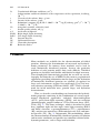
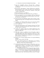
Chapter 10
Estimation of Intrinsically Disordered Protein Shape
and Time-Averaged Apparent Hydration in Native
Conditions by a Combination of Hydrodynamic Methods
Johanna C. Karst, Ana Cristina Sotomayor-Pérez,
Daniel Ladant, and Alexandre Chenal
Abstract
Size exclusion chromatography coupled online to a Tetra Detector Array in combination with analytical
ultracentrifugation (or with quasi-elastic light scattering) is a useful methodology to characterize hydrodynamic properties of macromolecules, including intrinsically disordered proteins. The time-averaged
apparent hydration and the shape factor of proteins can be estimated from the measured parameters
(molecular mass, intrinsic viscosity, hydrodynamic radius) by these techniques. Here we describe in detail
this methodology and its application to characterize hydrodynamic and conformational changes in proteins.
Key words: Molecular mass, Intrinsic viscosity, Protein shape, Time-averaged apparent hydration,
Protein hydration, Size exclusion chromatography, Static light scattering, Dynamic light scattering,
Analytical ultracentrifugation, Online viscometer
Abbreviations
M
T
C
dn=dc
dA=dc
½ n
d
f =f 0
f
f0
RH
R0
VH
Molecular mass, g/mol
Absolute temperature, K
Protein concentration, mol/L (M)
Refractive index increment, mL/g
Absorbance increment, L/g cm
Intrinsic viscosity, mL/g
Hydrodynamic shape function, viscosity increment, Simha–Saito shape factor, unitless
Time-averaged apparent hydration, gH2 O =gprotein
Translational frictional ratio of the protein, including shape and hydration parameters
Frictional coefficient of the protein, g/s
Frictional coefficient of an anhydrous sphere of the mass of the protein, g/s
Hydrodynamic radius of the protein, cm
Radius of an anhydrous sphere of the mass of the protein, cm
Hydrodynamic volume calculated from the RH, cm3
Vladimir N. Uversky and A. Keith Dunker (eds.), Intrinsically Disordered Protein Analysis:
Volume 2, Methods and Experimental Tools, Methods in Molecular Biology, vol. 896,
DOI 10.1007/978-1-4614-3704-8_10, # Springer Science+Business Media New York 2012
163
164
Dt
s
r
kB
NA
n
a=b
RALS
LALS
IP
DP
UV
RI
J.C. Karst et al.
Translational diffusion coefficient, cm2/s
Sedimentation coefficient obtained at the temperature of the experiment, Svedberg,
1013 s
Viscosity of the solvent, Poise: g/cm s
Density of the solvent, g/mL
Boltzmann’s constant, erg/K (KB: 1.38065 1016 erg/K, with erg: g cm2/s2 ¼ 107 J
1.38065 1023 J/K)
Avogadro’s number, molecules/mol
Partial specific volume, mL/g
Axial ratio of ellipsoid
Right Angle Light-Scattering
Low Angle Light-Scattering
Internal Pressure
Differential Pressure
Ultraviolet absorption
Refractive Index
1. Introduction
Many methods are available for the characterization of folded
proteins, allowing the determination of structural and hydrodynamic parameters. In contrast, fewer methods can be used to
study intrinsically disordered proteins, because the particular
behavior of such proteins makes their study difficult. Unfolded
proteins are hydrated and flexible with limited residual structure.
These biophysical characteristics preclude the use of X-ray crystallography and limit the use of NMR. In this context, experimental
approaches providing information on the shape and the hydration
of intrinsically disordered proteins are valuable. As opposed to
large-scale instruments required for small-angle X-ray and neutron solution scattering (SAXS and SANS), SEC-TDA is a benchmark for in-lab molecular mass, protein shape, and hydration
determination.
Here, we describe a methodology to characterize the hydrodynamic properties consisting in the combination of several experimental biophysical approaches: analytical ultracentrifugation
(AUC), quasi-elastic light scattering (QELS), and size exclusion
chromatography coupled online to a Tetra Detector Array (SECTDA) (Fig. 1). This latter technique, which is described in detail
here, combines right and low angles static light-scattering (RALS
and LALS) detectors, a spectrophotometer (UV), a refractometer
(RI), and pressure transducers (differential pressure (DP) and internal pressure (IP)) (Fig. 2). Importantly, this methodology allows
the characterization of intrinsically disordered proteins in solution
and in native conditions and provides an estimation of their hydrodynamic parameters, such as shape and hydration.
10
Estimation of Intrinsically Disordered Protein Shape. . .
Degasser
Pump
Solvent
Oven and columns
1.00
1.00
UV detector
Light scattering
detector
165
Autosampler
Injection
loop
1.00
Refractometer
1.00
Wastes
Viscometer
Fig. 1. Scheme of size exclusion chromatography system connected online to a Tetra
Detector Array and controlled by a GPCmax module (Viscotek Ltd., a Malvern Company).
The GPCmax module provides an integrated solvent pump, an autosampler, and a
degasser. The Tetra Detector Array contains a UV detector, a static light-scattering cell,
a differential refractive index (RI) detector, and a four-capillary differential viscometer. All
the detectors reside within a temperature-controlled compartment. It is noteworthy that
the linkup of an online QELS instrument would allow the acquisition of all hydrodynamic
parameters (M, RH, ½) with a unique sample injection.
Fig. 2. Schematic diagram of differential viscometer (Viscotek Ltd., a Malvern Company).
It consists of a four-capillary bridge design, developed by Dr. Max Haney. The four
capillaries are arranged in a balanced bridge configuration, analogous to the Wheatstone
bridge commonly present in electrical circuits. Differential pressure transducers measure
the pressure difference (DP) across the midpoint of the bridge and the pressure difference
IP from inlet to outlet. A delay column is inserted in the circuit to create the differential
pressure (providing a reference flow of solvent during elution of the sample).
Molecular mass and intrinsic viscosity are measured by
SEC-TDA. The protein concentration is determined using the photometer or the deflection refractometer. The static light-scattering
signals combined with the protein concentration provide online
measurements of the molecular mass (M) of each eluting species,
whereas differential viscometer measurements in combination with
protein concentration provide their intrinsic viscosity (½) values.
The hydrodynamic radius of the macromolecule, RH , is obtained
166
J.C. Karst et al.
either by the sedimentation coefficient (s) value determined by
AUC, or by using the translational diffusion coefficient (Dt) determined by QELS. From the hydrodynamic parameters (M, ½, RH )
measured by these techniques, we can ascribe the respective contributions of hydration and shape factor (viscosity increment) to the
intrinsic viscosity value.
The methodology described here has been shown to be useful
for the studies of intrinsically disordered proteins, protein/ligand
interaction (1, 2), protein/protein interaction (3, 4) and proteins
exhibiting anomalous behavior (5, 6).
2. Materials
1. A gel filtration column of appropriate fractionation range for
the samples of interest.
2. A gel filtration buffer that is compatible with both the column
and the sample (see Note 1).
3. Calibration standards (see Note 2):
(a) NIST-1923 Polyethylene Oxide 22 KDa (PEO from Viscotek PolyCalTM TDS-PEO-N at 4 g/L).
(b) BSA (SIGMA A0281 at 2 g/L).
4. A GPCmax module or a similar instrument that provides an
integrated solvent pump, an autosampler and a degasser
(Fig. 1). It can be controlled manually or using the OmniSEC
software.
5. A tetra detector array model 302 (Viscotek Ltd., a Malvern
Company) or a similar instrument that consists of a UV detector, a differential refractive index (RI) detector, a four-capillary
differential viscometer (Fig. 2) and a static light-scattering cell
with two photodiode detectors at 7 for low angle (LALS) and
at 90 for right angle laser light scattering (RALS) (Fig. 1).
All the detectors reside within a temperature-controlled
compartment (see Note 3).
3. Methods
3.1. Data Acquisition
1. Filter all solutions using a 0.22-mm filter to degas and remove
any small particles that may clog the column frit (see Note 4).
2. Change the RALS filter to avoid injection of column particle in
the static light-scattering cell.
3. Purge the pulse dampener.
4. Switch on the TDA electronic part, the laser source and the UV
detector (see Notes 5 and 6).
10
Estimation of Intrinsically Disordered Protein Shape. . .
167
5. Open the OmniSEC software (Viscotek Ltd., a Malvern
Company) and follow the general procedures described in the
user manual.
6. In the panel “tool/options,” choose a folder to save your files.
Enter parameters such as time and volume of an experimental
run, file name format, and detectors sensitivity in the panel
“acquire/configuration.”
7. Indicate the flow rate (see Note 7).
8. Select the minimum and maximum pressure (see Note 8).
9. Wash out ethanol 20 % (in water) from the GPCmax-TDA with
water (0.1 mL/min) and purge the Refractometer and Viscometer detectors (see Note 9).
10. Wash extensively the Hamilton syringe and its needle as well as
the injection loop of the autosampler with water and then with
buffer.
11. Equilibrate the GPCmax-TDA with at least 60 mL of buffer
(0.5 mL/min) and examine the baselines (see Note 10).
12. Start a quick run.
13. Purge the Refractometer and Viscometer detectors for 5 min
with buffer and repeat the operation until the displayed values
become stable (see Note 9).
14. Connect the column online; the column should have been
previously equilibrated with at least two column volumes of
buffer (see Note 11).
15. When the system is equilibrated, flat all baselines until an
acceptable signal/noise value is reached (see Note 10). Then,
turn off the flow, wait until the IP baseline is flat and reset the
Inlet Pressure Transducer by pushing the zero button on
the instrument (see Note 12).
16. Measure the viscometer bridge balance by using the following
formula:
Specific viscosity: 4DP/(IP-2DP)
The value should be below 0.03. The bridge is very well balanced for a specific viscosity value below 0.01 (i.e., 1 % of
difference across the viscometer bridge).
17. Clarify and degas the samples using a 0.22-mm filter and/or by
centrifugation (10,000 g for 10 min). Vials, containing the
sample, can be inserted at defined numbered positions in
the autosampler (see Note 13).
To determine M and ½ (and subsequently shape and hydration), a concentration of 2 g/L is required for a folded protein,
whereas 0.5–1 g/L is enough for an intrinsically disordered
protein, as ½ of such proteins is higher. To determine the
molecular mass only, a concentration around 0.5 g/L is enough.
168
J.C. Karst et al.
18. Create an analytical sequence in the software by listing the
injections to be realized: standards (BSA, PEO), sample injections, and finally standards again. Indicate the sample names,
concentrations, volume, number, and the order of sample
injections (see Note 14).
19. Start the sequence.
20. At the end of a sequence, replace the buffer from all the system
by water. Make purges of the Refractometer and Viscometer as
described in (11). Then store the system in filtered and
degassed 20 % ethanol (in water).
3.2. Data Processing
3.2.1. Calibration
Standards are used for TDA internal constant calibrations. BSA is
employed to calibrate the conversion from static light scattering to
molecular mass, as this protein is commonly used as a reference in
numerous biochemical applications. However, as its intrinsic viscosity is low, PEO can be used to calibrate both M and ½ parameters (see Note 2). Then, BSA injections are used to validate the
method.
Polypeptide concentrations can be determined using the photometer (UV) and/or the deflection refractometer (RI). RALS
and/or LALS data combined with the protein concentrations
(UV or RI) provide the molecular mass, while the differential
viscometer measurements (Differential Pressure, DP), in combination with the protein concentrations provide the intrinsic viscosity.
1. Open a file of standard for calibration.
2. For each detector, add the baselines automatically with
OmniSEC. If necessary, modify their positions manually and
note the noise (in Volt).
3. Surround the monomeric species by the integration limits on
all channels.
4. Create a method, in which you indicate all parameters
concerning the standard (dn/dc, dA/dc, MM, ½. . .) (see
Note 2). Click the box “Calculate Concentration from Detectors.” Two different methods can be created, one using the
refractometer (RI) and the other using the photometer (UV) as
detector to determine the sample concentration.
5. Press the button “calibration” and save the method.
6. Check the calibration constant values (see Note 15).
7. Test the calibration with the same standard file as sample and
with other injections of standard. If the standard changes, do
not forget to change the parameters (dn/dc, dA/dc. . .) in the
“sample parameters” window.
10
169
1. Open a sample file.
2. Determine the baselines automatically on all channels with
OmniSEC. If necessary, modify their position manually.
3. Place the integration limits on all channels by surrounding the
entire elution profile, from the void volume to the salt elution,
or restrict the window to the area of interest.
4. Open the appropriate method depending on the selected
detector used to determine the concentration (UV or RI).
Enter dn/dc and dA/dc of the protein in the “sample parameters” window.
5. Start analysis by pressing the button execution: the software
computes molecular mass and intrinsic viscosity of the macromolecule (see example given in Fig. 3).
a
160
50
16
12
8
40
120
30
80
20
RI signal, mV
RALS signal, mV
20
Differential pressure, mV
40
4
10
0
0
0
Molecular mass, KDa
b
Intrinsic viscosity, ml/g
3.2.2. Protein Parameters
Determination
Estimation of Intrinsically Disordered Protein Shape. . .
100
10
1
9
10
11
12
13
retention volume, ml
Fig. 3. Typical traces of a protein analyzed by size exclusion chromatography connected
to a tetra detector array. (a) Deflection refractometer (bold continuous line), right angle
light scattering (thin continuous line) and differential pressure (dotted line) chromatograms. (b) The molecular mass (black line) and intrinsic viscosity (grey line) are computed
with the OmniSEC software (Viscotek Ltd., a Malvern Company). This figure shows typical
chromatograms from the apo-state of the RD protein (1), an intrinsically disordered
protein (13).
170
J.C. Karst et al.
SEC-TDA
DP
IP
UV
RI
RALS
LALS
M
AUC
QELS
Biophysical techniques
S
Dt
Measured parameters
RH
Calculated parameters
Fig. 4. Determination of protein shape (n) and hydration (d) parameters. The molecular mass (M), the intrinsic viscosity ½,
and the hydrodynamic radius RH of the macromolecule determined by SEC-TDA, AUC, and/or QELS are required to
estimate protein shape and hydration.
6. Check the robustness of the results by testing the two different
methods (RI- and UV-based) if applicable, and different injections (volume or concentration) of the same protein sample.
3.3. Protein Shape and
Hydration Estimation
For the determination of protein shape and hydration, the molecular
mass (M), the intrinsic viscosity ½, the hydrodynamic radius RH and
the partial specific volume n of the protein are required (Fig. 4). The
hydrodynamic radius RH is calculated from the translational diffusion
coefficient measured by QELS using the Stock Einstein relation
RH ¼ ðkB T Þ=ð6pDt Þ or more accurately, using the Svedberg equation RH ¼ M ð1 rnÞ=ð6pNA s Þ with molecular mass determined
by SEC-TDA (see above) and sedimentation coefficient (s) determined by AUC (see Note 16). The partial specific volume (which
usually ranges between 0.69 and 0.75 mL/g) can be either experimentally determined by AUC equilibrium measurement or estimated
from the amino acids sequence with, for instance, the SEDNTERP
software (http://www.rasmb.bbri.org). The solvent viscosity and
density r can also be computed with the SEDNTERP software.
The intrinsic viscosity of a protein, ½ (7, 8), is expressed
according to the relation ½ ¼ nVs ¼ nðn þ d=rÞ (see Note 17).
The intrinsic viscosity is the product of (a) a hydrodynamic function,
the viscosity increment n, and (b) the swollen volume VS . A n value of
2.5 suggests that the protein adopts a spherical shape, while
10
Estimation of Intrinsically Disordered Protein Shape. . .
171
increasing values of n are indicative of ellipsoidal shapes. The swollen
volume is the sum of two volumic factors, i.e., the partial specific
volume, n, and the time-averaged apparent hydration of the
protein (d in gH2 O =gprotein ). The hydration parameter includes
the water molecules bound to the protein and the water molecules
entrained by the diffusion of the protein. Hydration corresponds to
the water molecules within the hydrodynamic volume, i.e., to the
water included in protein cavities and between the protein surface
and the plan of shearing (slipping plan).
Three approaches can be used to estimate protein shape and
hydration (see Fig. 4 and Note 18 for an example)
1. The shape factor n can be calculated using the Einstein viscosity
relation M ½ ¼ nVH NA (see Note 19) inverted to
n ¼ M ½=VH NA , where VH is the hydrodynamic volume
3
defined by VH ¼ 4pRH
=3. The viscosity increment is then
used to estimate the ratio (a=b ¼ #) of the semi-axes a and b
(with a > b) for an equivalent prolate or oblate ellipsoid. Harding and Colfen described polynomial equations that can be used
to convert the viscosity increment into the axial ratio value (9).
Solutions for triaxial ellipsoid have also been described (10).
3
The solution for a prolate ellipsoid (RH
¼ a b b with a > b
and a=b ¼ #) is given by a ¼ RH #2=3 and b ¼ a =# (or
b ¼ RH #1=3 ), while the solution for an oblate ellipsoid
3
(RH
¼ a a b with a > b and a=b ¼ #) is given by
b ¼ RH #2=3 and a ¼ # b (or a ¼ RH #1=3 ). Then,
from the intrinsic viscosity relation ½ ¼ nðn þ d=rÞ, the hydration d is calculated from the parameters ½, n and n according to
d ¼ ðð½=nÞ nÞr (see Note 20).
2. A second way to calculate protein shape and hydration is first to
determine the hydration ðdÞ from the experimental values of M, n
and RH using the relation M ðn þ dÞ ¼ VH NA . Then, the viscosity increment n is calculated with the intrinsic viscosity relation
n ¼ ½=ðn þ d=rÞ, providing the a/b ratio as described above.
3. As an alternative estimation of the semi-axial ratio (a=b ¼ #),
the Perrin hydrodynamic function P (11).can
h be calculatedi
according to the equation P ¼ ðf =f0 Þ
ððd=nrÞ þ 1Þ1=3
(12). For this purpose, the frictional ratio f =f0 and the previously determined hydration values d are combined. RH values
are used to calculate the frictional ratio f =f0 from the relation
f =f0 ¼ RH =R0 . The anhydrous radius R0 (by definition with
d ¼ 0), is defined by M n ¼ V0 NA ¼ ð4pR03 =3ÞNA, which gives
R0 ¼ ð3M n=4pNA Þ1=3 . An estimation of the semi-axial value
can be computed according to the polynomial equations
provided by Harding and Colfen (9). The shape factor estimated from the Perrin Hydrodynamic function is generally
lower than that obtained from the viscosity increment.
172
J.C. Karst et al.
4. Notes
1. It is recommended to work at neutral pH. Acidic buffers can
damage pressure transducers, whereas basic buffers can damage
quartz of the static light-scattering cell.
2. PEO and BSA parameters are the following:
PEO (Viscotek PolyCalTM TDS-PEO-N): its intrinsic viscosity
is 38.8 0.4 mL/g, its molecular mass is 22.411 g/mol
and its refractive index increment, dn=dc, is 0.132. It is
noteworthy that PEO cannot be used for a UV-method as
it does not absorb in the UV region.
BSA (SIGMA A0281): its intrinsic viscosity is 4 mL/g, its
molecular mass is 66,430 g/mol, its molar extinction coefficient (e) is 45,000 M1 cm1, dn=dc is 0.185 and dA=dc
is 0.667 L/g cm
The refractive index increment, dn=dc, is the slope of the
plot of the total scattered light (dn) as a function of sample
concentrations (dc). dA=dc is easily computed as
dA=dc ¼ e=M .
3. The instrument described in the present review was purchased
from Malvern (Malvern, UK). Other companies, e.g., Wyatt
Technology, sell similar apparatus.
4. Buffers must be degassed before use to prevent air bubbles
from becoming trapped in the pump, column, or detectors.
5. TDA power supply should not be switched off; it controls the
temperature of the oven that must be comprised between 15
and 80 C and be at least 3 C higher than the room (or refrigerated cabinet) temperature to ensure thermal stability.
The GPCmax system must be switched on in order to let
the degasser pump functioning. Degasser pressure must be
comprised between 0.7 and 0.8 mbar.
6. With flow, the pressure on DP and IP detectors should not
exceed 2.5 V (2.5 kPa) and 100 mV (100 kPa), respectively.
7. The flow rate must be 0.1 mL/min for the transition from 20 %
ethanol to water. Flow rate during an injection is comprised
between 0.2 and 0.5 mL/min. The flow of the pump can be
adjusted at any time during operation by pressing the Pump
ON key and type the desired flow in the box. In any case, it
should not exceed 1.5 mL/min when the viscometer is
connected online (the IP detector limit pressure is 100 mV,
which corresponds to 100 kPa).
8. Pressure must be limited to that of the column, including the
backpressure of the system. If the pressure drops under or exceeds
the programmed pressure values, the pump stops automatically.
10
Estimation of Intrinsically Disordered Protein Shape. . .
173
9. Purges are performed in order to obtain optimum, flat baselines.
Purge time can be settled from the software. Do not make them
too long (from 2 to 5 min) to avoid damage of purge valves.
10. Baseline detector responses are approximately: RI (variable),
UV: 20 mV; RALS: 30–50 mV; LALS: 300–500 mV; IP:
5–6 mV (at 0.1 mL/min) to 25–30 mV (at 0.5 mL/min). It
is noteworthy that a lower value can indicate a leakage; DP:
20–100 mV, as a function of the flow rate. Baseline noise
should be around: IP: 0.02–0.04; DP, RALS, RI, and UV:
0.1; and LALS: 0.5 mV.
11. It is better to equilibrate the column with water and then with
buffer before connecting it to the GPCmax system in order to
avoid injection in the detectors of particles that may come out
from the column.
12. The IP measurement is treated as an “absolute” measurement
by the data system, unlike the others signals, which are
baseline-corrected. For this reason, the IP must never be zeroed with the flow on.
13. Each vial is accessible to a needle, which can take a defined
volume of sample and inject it onto the column for analysis.
Put in the vial a higher volume than the one required because
you have to take into account the volume (1) lost in the capillar
during loop loading (typically, 50 mL) and (2) required to fill the
space between the bottom of the vial and the extremity of the
needle (this volume is dependent on the shape of the vial used).
14. At least three injections of different concentrations (0.5; 1;
2 g/L) or different volumes (100; 150; 200 mL) must be
performed for each sample. Usually, two or three injections of
each standard are performed at the same volume (150 mL) and
concentration (2 and 4 g/L for BSA and PEO, respectively) to
be sure of the signal and baseline stability, and the reproducibility of the data. If required, injections of variables volumes
(50–200 mL) can be performed in order to determine the dn/
dc of the samples (see Note 2).
15. Calibration constants values should range as following: RI and
UV: 1 106 to 20 106; RALS and LALS: 1 108 to
20 108; DP: 0.7–1.3.
16. The Svedberg equation is given by s ¼ M ð1 rnÞ=ð6pNA RH Þ,
where s is the sedimentation coefficient (S), M the molecular
mass (g/mol), n the partial specific volume (mL/g), and RH
the hydrodynamic radius of the macromolecule (cm). r and are the solvent density (g/mL) and viscosity (poise: g/cm s),
respectively.
17. The intrinsic viscosity relation is given by ½ ¼ nðn þ d=rÞ,
where ½ is the intrinsic viscosity (mL/g), n is the viscosity
increment (unitless), n the partial specific volume (mL/g),
174
J.C. Karst et al.
and d the hydration of the macromolecule (g/g). r is the
solvent density (g/mL).
18. Here is a theoretical example describing how to access to
hydrodynamic parameters from M, ½ and RH (Fig. 4). We
consider a protein with a molecular mass of 50,000 g/mol,
an intrinsic viscosity of 12 mL/g, a partial specific volume of
0.73 mL/g, a sedimentation coefficient of 3 S (3 1013 s)
and a translational diffusion coefficient of 5.6 107 cm2/s.
The macromolecule is studied at 25 C in Hepes 20 mM, NaCl
150 mM pH 7.4 of density 1.00382 g/mL and viscosity
0.00908 poise (or 0.00908 g/cm s).
We first calculate the hydrodynamic radius (RH ) using the
Svedberg equation:
RH ¼ M ð1 rnÞ=ð6pNA s Þ
with M in g/mol, r in g/mL, n in mL/g, in poise and s in
seconds.
RH ¼ 50; 000ð1 1:00382 0:73Þ
6p 0:00908 NA 3 1013
RH ¼ 4:32 107 cm
Alternatively, the hydrodynamic radius RH can be calculated from the translational diffusion coefficient measured by
QELS using the Stock Einstein relation
RH ¼ ðkB T Þ=ð6pDt Þ
with kB ¼ 1.38 1016 g cm2/s2K, T in Kelvin, in poise and
Dt in cm2/s.
RH ¼ 1:38 1016 298 6p 0:00908 5:6 107
RH ¼ 4:32 107 cm
From the RH , we calculate the hydrodynamic volume (VH )
of the macromolecule according to
3
VH ¼ 4pRH
=3
with RH in cm.
3
VH ¼ 4pð4:32 107 Þ =3
VH ¼ 3:38 1019 cm3
l
According to the first approach, the shape factor (the viscosity increment, n) is calculated using the Einstein viscosity relation:
n ¼ M ½=VH NA
with M in g/mol, ½ in mL/g, and VH in cm3.
10
Estimation of Intrinsically Disordered Protein Shape. . .
175
n ¼ 50; 000 12 3:38 1019 NA
n ¼ 2:95
The viscosity increment provides an estimation of the
ratio of the lengths of the semi-axes a and b of an ellipsoid
of revolution according to the polynomial equations
described by Harding and Colfen (9). A viscosity increment of 2.95 gives an axial ratio of 2.07. We can then
calculate the semi-axes a and b for an equivalent prolate
or oblate spheroid.
For a prolate ellipsoid (defined by a, b, b semi-axes):
a ¼ RH #2=3
b ¼ a=#
a ¼ 4:32 22=3
b ¼ 7=2
a ¼ 7 nm
b ¼ 3:5 nm
For an oblate ellipsoid (defined by a, a, b semi-axes):
a ¼ RH #1=3
b ¼ a=#
a ¼ 4:32 21=3
b ¼ 5:4=2
a ¼ 5:4 nm
b ¼ 2:7 nm
Finally, from the intrinsic viscosity relation, the hydration parameter is extracted:
d ¼ ðð½=nÞ nÞr
with ½ in mL/g, n in mL/g, and r in g/mL. n is unitless.
d ¼ ðð12=2:95Þ 0:73Þ1:00382
d ¼ 3:35 g=g
Altogether, these data indicate that the protein is elongated with an axial ratio of 2 and displays a high hydration.
l
The second approach is used to calculate first the hydration
parameter according to
d ¼ ððVH NA Þ=M Þ n
with VH in cm3, M in g/mol, and n in mL/g.
d ¼ ðð3:38 1019 NA Þ=50000Þ 0:73
d ¼ 3:34 g=g
The viscosity increment is then determined using
n ¼ ½=ðn þ d=rÞ
with ½ in mL/g, n in mL/g, d in g/g, and r in g/mL.
176
J.C. Karst et al.
n ¼ 12=ð0:73 þ 3:34=1:00382Þ
n ¼ 2:96
Then, the semi-axes a and b of an ellipsoid of revolution are estimated as described above.
l
Finally, the third approach is used
the Perrin
to calculate
hydrodynamic function P (P ¼ f =f0 Þ= ððd=nrÞ þ 1Þ1=3 )
as an alternative estimation of the semi-axial ratio using the
hydration previously calculated by the first and second procedures and the frictional ratio determined, according to
f =f0 ¼ RH =R0
R0 is the hydrodynamic radius of an anhydrous and spherical molecule with equivalent M and n and is defined as
3M n 1=3
R0 ¼
4pNA
with M in g/mol and n in mL/g.
19. The Einstein viscosity relation is given by M ½ ¼ nVH NA,
where M is the molecular mass (g/mol), ½ the intrinsic viscosity (mL/g), n the viscosity increment, and VH the hydrodynamic volume of the macromolecule (cm3).
20. The partial specific volume can be either calculated by AUC
equilibrium measurement or estimated with the SEDNTERP
software. An approximation of the n is enough for the calculation
of the hydration parameter. Indeed, n commonly ranges between
0.69 and 0.75 mL/g, which makes little changes to hydration
that can varies between 0.2 and 0.5 g/g for folded proteins, and
from 1 to 10 g/g for partially and intrinsically disordered proteins. These values are given as rough indications.
Acknowledgements
This work was supported by the Institut Pasteur (Grant PTR374),
the Centre National de la Recherche Scientifique (CNRS UMR
3528), and the Agence Nationale de la Recherche, programme
Jeunes Chercheurs (ANR, grant ANR-09-JCJC-0012).
References
1. Chenal A, Guijarro JI, Raynal B, Delepierre M,
Ladant D (2009) RTX calcium binding motifs
are intrinsically disordered in the absence of
calcium: implication for protein secretion.
J Biol Chem 284:1781–1789
2. Sotomayor Perez AC, Karst JC, Davi M, Guijarro JI, Ladant D, Chenal A (2010) Characterization of the regions involved in the
calcium-induced folding of the intrinsically disordered RTX motifs from the bordetella
10
Estimation of Intrinsically Disordered Protein Shape. . .
pertussis adenylate cyclase toxin. J Mol Biol
397:534–549
3. Sotomayor-Pérez AC, Ladant D, Chenal A
(2011) Calcium-induced folding of intrinsically disordered repeat-in-toxin (RTX) motifs
via changes of protein charges and oligomerization states. J Biol Chem 286:16997–17004.
4. Chenal A, Vendrely C, Vitrac H, Karst JC,
Gonneaud A, Blanchet CE, Pichard S, Garcia
E, Salin B, Catty P, Gillet D, Hussy N, Marquette C, Almunia C, Forge V (2011) Amyloid
fibrils formed by the programmed cell death
regulator Bcl-xL. J Mol Biol 415:584–599.
5. Chenal A, Vendrely C, Vitrac H, Karst JC,
Gonneaud A, Blanchet CE, Pichard S, Garcia
E, Salin B, Catty P, Gilltet D, Hussy N, Marquette C, Almunia C, Gorge V (2011) Amyloid fibrils formed by the programmed cell
death regulator Bcl-xL. J Mol Biol
415:584–599
6. Bourdeau RW, Malito E, Chenal A, Bishop BL,
Musch MW, Villereal ML, Chang EB, Mosser
EM, Rest RF, Tang WJ (2009) Cellular functions
and X-ray structure of anthrolysin O, a
cholesterol-dependent cytolysin secreted by Bacillus anthracis. J Biol Chem 284:14645–14656
177
7. Simha R (1940) The influence of Brownian
movement on the viscosity of solutions.
J Phys Chem 44:25–34
8. Harding SE (1997) The intrinsic viscosity of
biological macromolecules. Progress in measurement, interpretation and application to
structure in dilute solution. Prog Biophys Mol
Biol 68:207–262
9. Harding SE, Colfen H (1995) Inversion formulae for ellipsoid of revolution macromolecular
shape functions. Anal Biochem 228:131–142
10. Harding SE, Horton JC, Colfen H (1997) The
ELLIPS suite of macromolecular conformation
algorithms. Eur Biophys J 25:347–359
11. Perrin F (1936) Mouvement brownien d’un
ellipsoı̈de (II). Rotation libre et dépolarisation
des fluorescences. Translation et diffusion de
molécules ellipsoı̈dales. J Phys Rad 7:1–11
12. Squire PG, Himmel ME (1979) Hydrodynamics and protein hydration. Arch Biochem Biophys 196:165–177
13. Chenal A, Karst JC, Perez AC, Wozniak AK,
Baron B, England P, Ladant D (2010)
Calcium-induced folding and stabilization of
the intrinsically disordered RTX domain
of the CyaA toxin. Biophys J 99:3744–3753