1
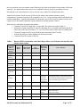
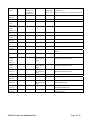
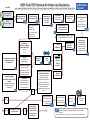
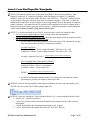
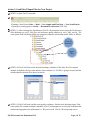
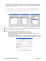
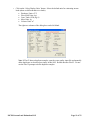
SOP Environmental Quality Assurance (EQA) Standard Operating Procedure Standard Operating Procedure: Estimation of Annual Tributary Stream Pollutant Loads with Flux32 Version 1.3 (Updated 09/20/2010; update 12/9/2011; update 9/13/2012) Author(s) Karen Jensen, updated by Emily Resseger Procedure Description Materials To calculate the annual pollutant loads for tributary streams using Flux32 software and water quality and flow data collected by the EQA – Environmental Monitoring and Assessment Unit or other project partners Flux32 software (most recent version). Download at ftp://ftp.usace.army.mil/pub/erdc/EL/Simple_Tools/FLUX_Updates/ • • • References Contents • • • • • • • Daily average flows (continuous record of measured and estimated daily flows) Event composite and grab sample flows and pollutant concentrations Manual_IR-W-96_2.pdf: “Simplified Procedures for Eutrophication Assessment and Prediction: User Manual”. William W. Walker. Instruction Report W-96-2. September 1996. Updated April 1999. U.S. Army Corps of Engineers SOP_Flux32_River_Load_Estimates_v1.3.docx MCES Steps for Flux Analysis_draft_200307.doc MPCA_FLUX32_Process_Checklist.doc Memo_20100714_WQ_Dataset_Review.docx Summary Tables Actions Summary: This SOP outlines the methodology for estimating annual pollutant loads for tributary streams from monitored daily average flow and grab/composite event sample chemistries using the U.S. Army Corps of Engineers’ software Flux32. Due to differences in input data processing and load estimation methodology, a separate SOP will be developed for estimating annual loads for monitoring stations located on the three major rivers (Mississippi, Minnesota, and St. Croix). Flux32 can easily be used mindlessly, resulting in inaccurate loads and statistics. It is crucial to use Flux32 mindfully with good technical judgment and familiarity with the stream or river dynamics, to ensure loads are accurate and defensible. This SOP is intended to provide typical procedures followed by MCES when calculating stream pollutant loads. Some stream sites or some years of data may be aberrant, and pollutant load calculation methodology must deviate from this SOP. All deviations from SOP procedures will be recorded in both the .TXT output file and in the results database “notes” field. Due to the flashy hydrology and associated complicated sample collection in tributary streams, MCES staff have determined that using three years of flow and chemistry data (i.e. the year of interest plus MCES Stream Load Estimation SOP Page 1 of 22 the two preceding years) to estimate annual loads typically reduces the statistical uncertainty of the load estimates. In comparison the three major rivers responds relatively slowly to precipitation events, allowing the river load estimates to rely on only one year of daily flow and chemistry data. Annual load estimates for the streams will be used in annual water quality summary reports, comprehensive assessment reports (to be completed every 3-to-5 years), special studies, and shared with external stakeholders. Annual load estimates for the major rivers will be used for similar activities and reports such as the annual benchmark report produced by the Metropolitan Council. Basic steps for estimation of annual loads include: o Creation of two Flux32 input files: average daily flow and water quality (Table 1) o Estimation of loads using Flux32 software, adjusting flow or seasonal stratification breaks to reduce the coefficient of variance (C.V.) to 0.2 or lower and to reduce slope in residual plots o Creation of output text files in specified format to document Flux32 results o Transfer the results to master database of stream load results o Creation of Flux32 Session (.FSS) File. Table 1: Historic MCES, Stakeholder, and Other Major Metro Area Tributary Stream Sites and Station Abbreviations Stream Name and Mile of Monitoring Station Bassett Creek 1.9 Battle Creek 2.2 Beltline Interceptor 0.5 Cannon River 11.9 Crow River 23.1 Crow River, South Fork 20.3 Elm Creek near Champlin Abbreviation (Site Code) Year Established Monitoring Staff / Data Owner Mississippi BS1.9 2000 Harrod Minneapolis Park and Rec Board Mississippi BA2.2 1995 Champion RWMWD Mississippi BELT0.5 1995 Champion RWMWD Mississippi CN11.9 2000 Harrod Dakota SWCD Mississippi CW23.1 2000 Harrod Wright County SWCD Mississippi CWS20.3 2001 Champion Carver County Environmental Services Mississippi ELM 1978 Not MCES cooperative station; USGS Station 05287890 operated in cooperation with Elm Creek Watershed Management Commission http://waterdata.usgs.gov/mn/nwis/ Fish Creek 0.2 Minnehaha Creek 1.7 Rice Creek 3.7 Mississippi FC0.2 1995 USGS and Elm Creek Watershed Management Commission Champion RWMWD Mississippi MH1.7 2000 Harrod Minneapolis Park and Rec Board Mississippi RC3.7 Unknown Rum River 0.7 Shingle Mississippi RUM0.7 1996 Rice Creek Watershed District Champion Not MCES cooperative station; Rice Creek Watershed District http://ricecreek.org/ Anoka Conservation District Mississippi SC-0 Unknown Shingle Not MCES cooperative station; belongs to Major Basin MCES Stream Load Estimation SOP Notes / Partners Page 2 of 22 Creek Outlet Vermillion River 2.0 Mississippi (Water Management Commission station name) VR2.0 Bevens Creek (Lower) 2.0 Bevens Creek (Upper) 5.0 Bluff Creek 3.5 Carver Creek 1.7 Credit River 0.9 Eagle Creek 0.8 Nine Mile Creek 1.8 Riley Creek 1.3 Sand Creek 8.2 Sand Creek – Scott County Ditch 10 Sand Creek – West Raven Willow Creek 1.0 Minnesota BE2.0 1989 Haire MCES Non-point Source Station Minnesota BE5.0 1992 Haire MCES Non-point Source Station Minnesota BL3.5 1991 Haire MCES Non-point Source Station Minnesota ca1.7 1989 Haire MCES Non-point Source Station Minnesota cr0.9 1989 Haire MCES Non-point Source Station Minnesota ea0.8 2000 Harrod Lower Minnesota Watershed District Minnesota nm1.8 1989 Haire MCES Non-point Source Station Minnesota ri1.3 2000 Harrod Minnesota sa8.2 1990 Pattock Riley-Purgatory-Bluff Creek Watershed District MCES Non-point Source Station Minnesota sd10 ~1994; Discontinued 2010 Pattock Operated in partnership with Scott SWCD. Station discontinued in 2010 Minnesota wr Pattock Operated in partnership with Scott SWCD. Station discontinued in 2010 Minnesota wi1.0 ~1994; Discontinued 2010 2000; Discontinued 2010 Harrod Dakota SWCD; Station discontinued in 2010 Browns Creek 0.3 Carnelian Marine 3.0 St. Croix br0.3 1997 Champion Washington Conservation District St. Croix cm3.0 Champion Washington Conservation District; station discontinued in 2010 Silver Creek 0.1 Valley Creek 1.0 St. Croix si0.1 1995; Discontinued 2010 1998 Champion St. Croix va1.0 2000 Harrod Washington Conservation District; site originally located at si0.7 Valley Branch WD, St. Croix Watershed Research Station MCES Stream Load Estimation SOP Creek Water Management Commission Shingle Creek Watershed Management Commission http://www.shinglecreek.org/wqlstrmon.shtml 1995 Champion Dakota SWCD Page 3 of 22 MCES Flux32 SOP Overview for Stream Load Calculations Input Files Note: Intended as guidance document only. Analyst must use good judgment and mindfulness to ensure proper calculation of loads with Flux32. Flux32 Average Daily Discharge Input Load Discharge and WQ Input Files Into Flux32 13 - 16 Flux32 Water Quality Input Set Date Filter (For Streams, use 3 calendar years) Examine data for proper loading and initial assessment Define Flux Settings (Units, Regression #6) 17 - 18 19 Method: 6 Regression (3) Discharge: cfs Flux Units: kg/yr Conc. Units: PPM (mg/L) Mass Units: kg Volume Units: m3 26 Examine Flow Weighted Concentrations from the Loading Summary Is the Method 6 concentration within 20% of Method 3-5 concentrations? No 24 Statistics can’t be met regardless of the stratification scheme Calculate Load using best judgment and carefully document observed problems or decide that load cannot be estimated. Note possible reasons in results worksheet (i.e. unexplained outlier, insufficient dataset) No? Are Methods 3-5 within 20% of each other? Yes 23 Export Flux32 Results to Load Summary Worksheet (Excel File) 27- 31 Consider Change to Regression Method 3- 5. Note that Time Series cannot be used with Method 3. 24 Discharge Stratification Export Flux32 Results (Annual, Monthly, and Daily Loads, Statistics) to text file Yes? Improve Diagnostic Statistics by Stratification Plot Residuals vs. Flow, Date, Month Are there breaks in season or discharge? If possible, improve residuals by stratification Date Stratification (Cannot Use Date Strat. With 3-yr stream data) Calculate Load 25 List Jackknife Are there samples that greatly affect load? If yes, is there a valid reason to eliminate the sample? 22-23 Examine relationship between Q / C (log) A strong relationship exists if R2 ≥ 0.75? Validate Load Calculation Check for Residual Outliers Are there are outlier samples which P<=0.05? If yes, is there a valid reason to eliminate the sample? 22 Examine distribution of samples vs. daily flows Do samples capture peaks? Season Stratification Check C.V. C.V. should be ≤ 0.3 (preferably CV≤ 0.2 ) 26 20 Examine Diagnostic Stats CV ≤ 0.3 (preferably CV ≤0.2) Residual R2 & Slope ≈ 0 Method 6 ≈ Methods 3-5 21 Plot Residuals vs. (Flow , Date, and Month) Optimum Residual Stats Slope =~ 0 R2 =~ 0 Choose Appropriate Stratification Type based on Acceptable Statistical Values Calculate Initial Loads (Single Strata) Flux32 Process Complete Save Flux32 Session File 32 33 = Indicates cited process step in associated MCES Flux32 Stream Load SOP document File = MCES_Stream_Flux32_Users_Diagram_v1.1.pptx; Updated 9/13/2012 by E. Resseger 13 - 16 Action 1: Create Flux32 Input File: Daily Average Flow (STEP 1) For streams: download daily average flows from http://environment/EQA/EMA/WaterQuality/ContStreamData.asp (STEP 2) Examine flow dataset for completion for the period of interest, with no missing data. Staff of the EQA-Environmental Monitoring and Assessment Unit should have estimated missing data to create continuous set of daily flows. (STEP 3) Create Excel spreadsheet using the following format or append new data to existing input file and update notes page to reflect addition of data. o Create two worksheets within file. First worksheet labeled “flow” on bottom tab; second worksheet labeled “notes” (STEP 4) Each Excel worksheet should use the following format or append new data to existing input file and update notes page. The notes worksheet should be updated when new data is added each year. o Cell A1 has no effect on Flux and should contain site description and any other relevant information. o Cell B1 should define the flow unites used (i.e. CFS, ft3/s or ft3/sec, m3/s, m3/sec, or CMS hm3/y or million m3/y) o Format “flow” worksheet as follows: o A B 1 Site description ft3/sec 2 Date Flow 3 01/01/99 10 4 01/02/99 15 C D Qualifier e Format “notes” worksheet as follows. This worksheet will be updated as new data is added each year. A B C 1 Site description 2 Date Note Author 3 05/26/09 Added 2008 data Kmj 4 05/28/10 Added 2009 data Kmj MCES Stream Load Estimation SOP D Page 5 of 22 (STEP 5) Name flow input file according to following naming convention: o Siteabbreviation_latestyearofdata_flow.xls o Example: sa8.2_2008_flow.xls See example file: NATRES\Assessments\WQ_Load_Calculations\Sample_files\Sample_stream_flux32_flow_in put_file.xls Note: if adding new data to existing Flux32 input file, update Notes page and resave file in appropriate file folder with new file name appropriate for the most recent data added (eg. sa8.2_2010_flow.xls). Do not alter existing files, as they will be used to recreate loads if questions/problems arise in future. MCES internal file structure for the storage of Flux32 files is outlined in the Annual WQ Assessment SOP File Location: \NATRES\Assessments \Documents\SOP\SOP_WaterQuality_Assessment_V1.doc MCES Stream Load Estimation SOP Page 6 of 22 Action 2: Create Flux32 Input File: Water Quality (STEP 6) Download verified water quality data from EIMS or Water Quality Database. Data flagged as censored (‘X’) should be excluded, while data flagged as suspect (‘S’) should be included. Make sure file includes fields “flux date” and “flux flow”. “Flux date” is either the date of grab sample collection or the mid-storm date for composite samples. “Flux flow” is either the instantaneous sample flow for grab samples or the average sample flow for the period of composite sample collection. Also make sure the file includes field comments to be used if a sample point is being assessed as an outlier to be removed from analysis. Additional assistance in processing data can be found in Memo_20100714_WQ_Dataset_Review.docx (STEP 7) To avoid calculation error in Flux32, make sure there is only one sample per date o For two (or more) grab samples per date: average flows and concentrations o For one grab and one composite per date: delete the grab sample and keep composite results o For two (or more) composite samples per date: → Are the samples representing portions of the same storm? If so, estimate the average flow and concentration for the two composites as follows: Average Flow Flow: Composite 1 Volume: Event Length (Seconds) * Flux flow (cfs) = (ft3) Composite 2 Volume: Event Length (Seconds) * Flux flow (cfs) = (ft3) Average Composite Flow (cfs) = Flow Weighted Mean Concentration (FWMC): Composite 1 Mass = Flow * Concentration Composite 2 Mass = Flow * Concentration ∑ Sample Volume = Total Volume (ft3) FWMC = Σ Σ → Are the two composites separate events? If so, delete one event and note in data processing log, as only one sample is allowed per date. (STEP 8) Create an Excel spreadsheet with separate worksheets for notes and water quality (wq). This file will serve as the Flux32 Water Quality Input File. (STEP 9) Create two worksheets. First worksheet labeled “wq”; second worksheet labeled “notes” o Format “wq” worksheet as follows. o Cell A1 has no effect on Flux and should contain site description and any other relevant information. o Cell B1 should define the concentration units (ppb, mg/L, or ppm) o Cell C1 should define the sample flow units (cfs, ft3/s, m3/s, hm3/yr) MCES Stream Load Estimation SOP Page 7 of 22 o For ease of future data analysis, some water files will also contain fields for turbidity in NTU and NTRU. Obviously, a turbidity load cannot be calculated with Flux. A B 2 Site description Date 3 4 1 C D E F G Concentration Flow units units Sample_flow Field_data_ID Type TP TSS NO3 01/01/99 10 345678 grab 0.105 549 4.5 01/02/99 15 356780 composite 0.255 1549 1.2 (STEP 10) Format “notes” worksheet as follows. If modifications are made to an existing water quality dataset, the changes should be reflected in this page. A B C D E Data filename Author 1 Site description 2 Date Note 3 05/26/09 Added 2008 data Data download date 05/13/09 4 05/28/10 Added 2009 data 05/20/10 F Allstreams_2008 Kmj .xls Allstreams_2009 Kmj .xls (STEP 11) Name flow input file according to following naming convention: Siteabbreviation_latestyearofdata_wq.xls Example: sa8.2_2008_wq.xls See example input file: NATRES\Assessments\WQ_Load_Calculations\Sample_files\Sample_stream_flux32_wq_input_fi le.xls Note: if adding new data to existing Flux32 input file, update Notes page and resave file in appropriate file folder with new file name appropriate for the most recent data added (eg. sa8.2_2010_wq.xls). Do not alter existing files, as they will be used to recreate loads if questions/problems arise in future. MCES internal file structure for the storage of Flux32 files is outlined in the Annual WQ Assessment SOP. File Location: NATRES\Assessments\Documents\SOP\SOP_WaterQuality_Assessment_V1.doc MCES Stream Load Estimation SOP Page 8 of 22 Action 3: Load Flux32 Input Files for New Project (STEP 12) Open Flux32 executable If starting a New Project: Data → Read → New Sample and Flow Data → New Stratification If opening an existing project: Session → Resumed Saved Session (.FSS File) (STEP 13) After selecting New Stratification, Flux32 will prompt the user to locate the file directory of the discharge (eg. sa8.2_2009_flow.xls) and water quality samples (eg. sa8.2_2009_wq.xls). The water quality load calculation folders are organized within the Assessment master folder, as follows: Year of Interest Input Files (STEP 14) Flux32 will first read in the daily discharge worksheet. If the daily flow file contains multiple worksheets, the user must indicate what worksheet (i.e. FLOW) is going to be used and the column identifier that the flow data is located in. (STEP 15) Flux32 will next read the water quality worksheet. Similar to the discharge input, if the water quality file contains multiple worksheets, Flux32 will prompt user to select the worksheet that contains the appropriate site information (i.e. WQ) to be used. Flux32 will next prompt user to MCES Stream Load Estimation SOP Page 9 of 22 select SAMPLE_FLOW Field from a list of fields. For stream load estimation, the user should select the field named SAMPLE_FLOW from the list, as each sample should have an associated composite or instantaneous flow. Note: This differs from river load estimation. MCES typically uses the daily average flow to represent the sample flow when calculating major river loads. Most major river samples are collected as grab samples and the major river flows change relatively slowly – thus use of daily average flow as an approximation of sample flow is appropriate. (STEP 16) Flux32 will next prompt user to select the FLUX CONSTITUENT Field from a list of fields. Select field name of parameter to be estimated. (STEP 17) Flux32 will then prompt user to complete the following: o Enter/Modify Site Name: Enter appropriate site name and location. o Confirm input data. Examine the page to make sure number of daily flows and number of samples seems appropriate o Confirm appropriate values for unit conversion. Ensure the conversion factors are correct: 0.894 if using cfs; 1,000 if using mg/l. Use dropdown menus to change values, if necessary. MCES Stream Load Estimation SOP Page 10 of 22 o Click on the ‘Select Display Units’ button. Select the default units for estimating stream loads (these are different than river loads). Discharge Units: CFS Flux (load) Units: kg/y Conc. Units: PPM (mg/L) Mass Units: kg Volume Units: m3 The right two columns of the dialog box can be left blank. Note: If Flux32 detects duplicate samples, open the water quality input file and manually delete duplicates as described previously in this SOP. Reload data into Flux32. Do not use the Flux32 prompts to delete duplicate samples. MCES Stream Load Estimation SOP Page 11 of 22 Action 4: Estimate Stream Loads with Flux32 (STEP 18) Set initial default settings o Select Method #6: Method → 6 Regression (3): Daily log c/log q, adj Note: Method 6 is the preferred calculation method as it designed for use with the time series function, which will be used later in this SOP to save data output for yearly, monthly, and daily time steps. (If a load is unable to be calculated using Method 6, the user may use an alternate method. A complete explanation of the Method 6 departure criteria is outlined in Step 26.) o Name Session Title: Title→Session Title Name session using stream name and monitoring location mile, for example Vermillion River 2.0. (STEP 19) Examine entire dataset to ensure proper loading and assess potential stratification schemes. Confirm that flow data are complete without breaks and that number of samples indicated seems appropriate. Examine plots for concentration vs. flow or concentration vs. season relationships. (STEP 20) Set Data filter/screen to include only data period of interest. o Data → Screen/filter data → Apply Date & Value screens → Sample Date Range: For stream sites, three calendar years of data are used to develop regression equations used in estimating loads. The max date should be set to the last day of the year of interest (12/31/2009 when estimating 2009 loads). The min date should be set to the first day of third previous year (for estimating 2009 loads, the min date would be 01/01/2007). If the analyst is calculating the load for the first year of monitoring data, it is necessary to use the two following years to create a three-year record. For example, if 2005 is the first year of monitoring, the 2005 load will be calculating using data from 2005-2007. The load for the second year of monitoring (2006) must also be calculated using 2005-2007. Similarly, if a year of data is missing due to equipment failure, use judgment to define three year period of data. For example, if loads are to be calculated for 2007, but the station was inoperative during 2006, the analyst may decide to use 2004, 2005, and 2007 as the three year period. Of course, the date range will be noted in the output .TXT file and the output database. MCES Stream Load Estimation SOP Page 12 of 22 o Data → Screen/filter data → Apply Date & Value screens → Flow Date Range: For stream sites, three calendar years of data are used. The max date should be set to the last day of the year of interest (eg. 12/31/2009 when estimating 2009 loads). The min date should be set to the first day of third previous year (for estimating 2009 loads, the min date would be 01/01/2007). See above paragraph on Sample Date Range for more guidance setting dates for unusual circumstances. Note: Once dates are changed using data screen, do not simply change the dates again to refilter data, as an error occurs and data will not be loaded properly. To reset dates: Data → Screen/filter data → Apply Date & Value screens → Reset and then repeat date filter process described above. (STEP 21) Examine filtered dataset to ensure proper loading and assess potential stratification schemes. Make sure flow data is complete without breaks and that number of samples indicated seems appropriate. Examine plots for concentration vs. flow or concentration vs. season relationships. Look for logical breaks in relationship where stratification breaks could be made. o Plot → Conc → vs. Flow > linear o Plot → Conc → vs. Flow > log o Plot → Conc → vs. Date o Plot → Conc → vs. Month MCES Stream Load Estimation SOP Page 13 of 22 o Verify the distribution of samples versus daily flows to ensure that the samples capture the peaks. This information can be obtained using the Quick Plot tool on the main screen of Flux32. While there are no specific criteria for appropriate flow vs. concentration or the distribution of samples to daily flows, weak relationships can hinder the user’s ability to calculate loads and can be used to justify the inability to calculate a load (Step 26). (STEP 22) Calculate initial loads using one stratum o Calculate → Loads Examine Flow and Load Summary output. In particular: • Do the daily flow statistics agree with the dates selected in the data filtering process (#1 below)? • Is the Flux (kg/y) similar between the various statistical Methods 2-6 (#2 below)? Is the Method 6 C.V. < 0.2? How do the Method 6 results compare to the other methods (#3 below)? • The inability to meet the following criteria does not necessarily mean a load cannot be calculated; however, additional modifications to the data as outlined in subsequent steps (i.e. stratification, method change) may be needed. #1 #2 #3 MCES Stream Load Estimation SOP Page 14 of 22 (STEP 23) Examine initial qualitative (graph) and quantitative (statistics) diagnostics. o Plot → Residuals → vs. Flow → o Plot → Residuals → vs. Date → o Plot → Residuals → vs. Month → Note: Input data and associated loads for streams may be influenced by flow and by date/season, in which case the flow residual plot may look acceptable (no slope, high slope significance, low R2) while the date or month residual plots may be sloped, indicating a date or seasonal bias. Flux32 does not include both date and flow relationships in the load estimates; however, the USGS load estimation tool (LOADEST) does have that capability. With Flux32, the user must choose to either minimize flow residuals or minimize date/seasonal residuals using stratification. (STEP 24) Upon examining the initial load results using a single stratum, the user has the option of assigning multiple strata based on discharge or seasonal / date. The objective is to reduce the C.V., minimize residual slopes, and achieve convergence between flux and concentration for Methods 2-6. o Stratify data: Data → Stratify → On Flow On Hydrograph Date Stratification is not an option for On Season stream load calculations, since three years of data are used to develop statistics. On Date o On Flow Stratification: Typically relies on two strata (split at Qmean) or three strata (split at ½ Qmean and split at 2x Qmean). Upon choosing one of the flow strata, the user can then manually edit the strata boundaries through numeric or graphical means. If the user would prefer to manually enter all of the strata breaks, use Data → Stratify → On Flow → Other. o On Season Stratification: Stratification breaks often correlate with winter (mid-October – January), spring (February – mid May), summer (mid-May – mid-August), and fall (midAugust – mid-October). Examining the graphical interface will assist the user in appropriately identifying strata breaks. MCES Stream Load Estimation SOP Page 15 of 22 (STEP 25) Check diagnostic plots and statistics: Once strata breaks are set, go through the following process to check diagnostic plots and statistics. Table 2 outlines diagnostic tests and goals. Table 2: Flux32 Diagnostics for Load Calculation Acceptability Flux32 Diagnostic Plot or Statistic Description Optimum Goal Plot → Residuals → vs. Flow, Examine residual plots for bias; vs. Date, vs. Month Click “Show Stats” on plot. Often bias can be eliminated for Flow or Date, but not both No slope (slope ≈ 0) Minimize R2 (R2 ≈ 0) Maximize Slope Significance ( ≈1) Calculate → Loads Flow weighted concentration estimate for Method 6 should be within 20% of Methods 3-5. C.V. range 0 - 0.1 (Excellent) 0.1 - 0.2 (Good) > 0.2 (Fair) > 0.3 (Generally unacceptable) Provides information about distribution that may help with data interpretation Creates summary table of load by method; also gives C.V. by method Calculate → Compare Sample Provides a variety of statistics Flow with Total Flow comparing sample flow with total Distribution flow distribution List → Residuals → Outliers Provides lists of statistical outliers (P<=0.050) List → Jackknife Table Jackknife procedure systematically deletes individual samples and recalculates load without that sample, then presents % change in load estimate. Can provide information about optimizing sample collection during future efforts. List → Breakdown by Stratum and Optimum Sampling Outliers should only be deleted with some evidence of problem with sample. Deletion of outliers can greatly affect load estimates. If outlier is deleted, be sure to note in output text file. Look through table and identify individual samples that greatly influence load estimate. May add in interpretation or aid in elimination of outliers. Can aid in data interpretation. (STEP 26) If diagnostics are acceptable (based on calculation method and statistical relationships), proceed to Step 27. If diagnostics are unacceptable, first attempt to adjust stratification breaks or change stratification scheme (for example, change from flow stratification to seasonal stratification). Evaluate outliers and jackknife to identify aberrant samples. Outliers should be deleted cautiously and only with reason; always make note of deleted outliers in output file. o As a general guideline, if the Method 6 flow weighted concentration is greater than +/- 20% of Methods 3-5 concentrations/loads, then use of Method 6 may be abandoned for an alternative methods (Methods 3 – 5, preferably Method 4 or 5). It is advised not to use the time series function with Methods 2 or 3. The user will therefore only be able to cite annual modeled loads (rather than monthly or daily). Dave Soballe of ACOE reports that Method 6 MCES Stream Load Estimation SOP Page 16 of 22 time series (calendar year, monthly, and daily results) are most accurate as long as the C/Q relationship has a high r2 (~0.75) or if Methods 2-6 converge on a similar result. Analyst notes on method selection should be included in both .TXT output file and output database “notes” field. o If none of the methods produce a statistically significant load (C.V. > 0.3 and loads do not converge on similar value) and indicators exist such as weak representation of samples to the daily flow regime and poor residual statistics regardless of stratification scheme, you may not be able to calculate a load for the specified calendar year. If there is some variability between the flow weighted concentrations of Methods 3-5, but all indicators suggest an appropriate dataset, proceed will load calculation and make note of variability. (STEP 27) Once diagnostics are evaluated and optimized, calculate final loads and create output file as defined in Action 5. MCES Stream Load Estimation SOP Page 17 of 22 Action 5: Create Output File (STEP 28) Open text editor like “Notepad” or “Notetab Light” (STEP 29) Enter introductory information as follows: Line 1: Site name, parameter, year of interest Line 2: Date of analysis and analyst name Line 3: Version of Flux32 Line 4: Input file names Line 5: Stratification breaks Line 6: Outliers deleted Line 7: Notes Example Sand Creek 8.2 TSS loads for 2009 Date/analyst: 05/26/10; Karen Jensen Flux 32 Version: 1.1.2 (3/10/09) Flux32 input files: sa8.2_2009_flow.xls; sa8.2_2009_wq.xls Satrification breaks: 0-20 cfs, 20-120 cfs, 120-540 cfs Outliers deleted: Deleted one outlier (08/04/2009) Notes: Best agreement among methods 3-6. (STEP 30) Once above information has been added, cut and paste the following into the text file, in this order: Only paste the results for the year of interest to avoid future confusion. For example, if calculating 2009 loads, eliminate estimates for 2007 and 2008 (which would have been used as part of the three-year dataset to develop statistical relationships). o Calculate → Loads o To calculate time series loads (daily, monthly, calendar) Use 1 Day as Maximum Gap for Interpolation → Calculate → Series → Calendar Year (1 Day as Maximum Gap for Interpolation) → Calculate → Series → Monthly (1 Day as Maximum Gap for Interpolation) → Calculate → Series → Daily (1 Day as Maximum Gap for Interpolation) MCES Stream Load Estimation SOP Page 18 of 22 Example Notepad Output file: MCES Stream Load Estimation SOP Page 19 of 22 Time Series portion of NotePad output file. Note that 2007 and 2008 results have been deleted, leaving only year of interest (2009). (STEP 31) Save output file using the following naming convention: SiteCode_parameter_year.txt Example: CN11.9_NO3_2009.txt in the folder: NATRES\ Assessments\WQ_Load_Calculations\Output_Files\Streams\Text_Files (STEP 32) Load values and statistics are manually extracted and summarized within a historic stream loads database. The location of the MCES Stream Loads dataset is: NATRES\ Assessments\WQ_Load_Calculations\Output_Files\Streams\Streams_WQ_Load_Dataset.xlsx If additional load data is added to the Streams_WQ_Load_Dataset.xlsx the user should update the Notes worksheet. MCES Stream Load Estimation SOP Page 20 of 22 Information that needs to be added to the Streams_WQ_Load_Dataset.xlsx file is: o Site Code o Site Type o Parameter o Version (if input data is updated and the model is rerun, the output text file should be saved as SiteCode_Parameter_year_V#.txt, where # is run of the model. # should be indicated here) o Database Query Date o Analysis Period o Load Year o Stratification Scheme o Stratification Divisions o Calculation Method o Samples Excluded o Total Samples Used o Samples for Year of Interest o Annual volume (either in cfs or m3) o Model-Mass (kg) o Model-Conc (mg/L) o Interp-Mass (kg) o Interp-Conc (mg/L) o CV (Coefficient of Variation) o Updated By o Updated On o Comments (should match notes in text file) Columns shaded in blue are should calculate automatically. These calculations include: o o o o o o o o o o Site Name Major Watershed Muliple Versions? (yes or no) Output Text File Name Output Flux32 Session File Name Annual Volume (cfs) (calculated based on whether you enter volume in cfs or m3) 95% CI Upper Limit (kg) 95% CI Lower Limit (kg) Quality Check: Back-Calculate concentration (mg/L) Quality Check: Highlight if >3% diff The upper and lower confidence limits of the 95% confidence interval are calculated using the method cited within the Flux user’s manual entitled Simplified Procedures for Eutrophication Assessment and Prediction: User Manual (William Walker, 1999) as follows: Lower Limit value = Ym * e(-2 * CV) Upper Limit value = Ym * e(2 * CV) where Ym is the predicted mean value and CV is the error mean coefficient of variation. MCES Stream Load Estimation SOP Page 21 of 22 (STEP 33) Save Flux32 Session File using similar naming scheme as used in Step 31. o Session Æ Save This Session o Save output file using the following naming convention: SiteCode_parameter_year.txt. The file should be saved in NATRES\Assessments\WQ_Load_Calculations\Output_Files\Streams\Session_Files. Note that session file names cannot include “.” or “-“. Use only alpha-numeric characters and underscores in session file names. o Example: CN119_NO3_2009.FSS MCES Stream Load Estimation SOP Page 22 of 22