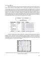
1
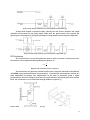
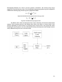
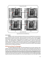
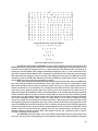
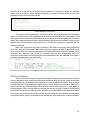
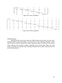
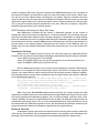
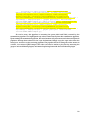
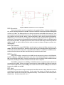
provides the EKF with linear acceleration and angular velocity, both in the body frame of
reference. With these several sensor measurements, predictions become much more accurate,
despite the low sampling rate of the visual odometry subsystem. More accurate predictions result
in more effective noise removal and therefor closer estimations of the systems true movement.
Listed below are the different equations, matrices, and vectors needed for the EKF. The
subset for each variable corresponds to the x, y, or z component of that variable. Px is the position
in the x direction. vx is the velocity in the x direction. ax is the acceleration in the x direction. θx is
the angle about the x-axis. 𝜃𝑥̇ is the change in the angle about the x-axis. Figure III.XVIII shows the
state and measurement vectors. The state vector shows all of the variables that are estimated and
the measurement vector shows all of the measurements that are received from the cameras and
IMU. Figure III.XI shows the observation versus estimation matrix. This matrix compares what
information is received from the cameras and IMU to the variables that are estimated. Figure III.XII
displays the state transition matrix of the system using the dynamic equations shown in Figure
III.XIII. The time step dt in these equations and matrices is determined by the update rate of the
IMU due to its much faster sampling rate than that of the visual odometry subsystem. The dynamic
equations listed below are in terms of the x-axis but can be extended to the y and z axes.
𝑃𝑥
𝑃𝑦
𝑃𝑧
𝑣𝑥
𝑣𝑦
𝑣𝑧
𝑎𝑥
𝑎
𝑥𝑘 = 𝑎𝑦
𝑧
𝜃𝑥
𝜃𝑦
𝜃𝑧
𝜃̇𝑥
𝜃̇𝑦
[ 𝜃̇𝑧 ]
𝑦𝑘=
𝑣𝑥
𝑣𝑦
𝑣𝑧
𝑎𝑥
𝑎𝑦
𝑎𝑧
𝜃̇𝑥
𝜃̇𝑦
[ 𝜃̇𝑧 ]
Figure III.X: State and Measurement Vectors
0
0
0
0
𝐻= 0
0
0
0
[0
0
0
0
0
0
0
0
0
0
0
0
0
0
0
0
0
0
0
1
0
0
0
0
0
0
0
0
0
1
0
0
0
0
0
0
0
0
0
1
0
0
0
0
0
0
0
0
0
1
0
0
0
0
0
0
0
0
0
1
0
0
0
0
0
0
0
0
0
1
0
0
0
0
0
0
0
0
0
0
0
0
0
0
0
0
0
0
0
0
0
0
0
0
0
0
0
0
0
0
0
0
0
0
0
0
1
0
0
0
0
0
0
0
0
0
1
0
0
0
0
0
0
0
0
0
1]
Figure III.XI: Observation vs. Estimation Matrix
29