Download User`s Manual PMM 8053B

NARDA
Safety
Test
Solutions
S.r.l. Socio Unico
Sales & Support:
Via Leonardo da Vinci, 21/23
20090 Segrate (MI) - ITALY
Tel.: +39 02 2699871
Fax: +39 02 26998700
Manufacturing Plant:
Via Benessea, 29/B
17035 Cisano sul Neva (SV)
Tel.: +39 0182 58641
Fax: +39 0182 586400
http://www.narda-sts.it
User’s Manual
PMM 8053B
SYSTEM FOR THE
ELECTROMAGNETIC FIELDS
MEASUREMENT
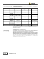
SERIAL NUMBER OF THE INSTRUMENT
You can find the Serial Number on the bottom cover of the instrument.
The Serial Number is in the form: 000XY00000.
The first three digits and the two letters are the Serial Number prefix, the last five
digits are the Serial Number suffix. The prefix is the same for identical instruments,
it changes only when a configuration change is made to the instrument.
The suffix is different for each instrument
Document 8053BEN-40918-3.16 – Copyright © NARDA 2014
NOTE:
® Names and Logo are registered trademarks of Narda Safety Test Solutions GmbH and L3
Communications Holdings, Inc. – Trade names are trademarks of the owners.
If the instrument is used in any other way than as described in this Users Manual, it may become unsafe
Before using this product, the related documentation must be read with great care and fully understood to
familiarize with all the safety prescriptions.
To ensure the correct use and the maximum safety level, the User shall know all the instructions and
recommendations contained in this document.
This product is a Safety Class III instrument according to IEC classification and has been designed to
meet the requirements of EN61010-1 (Safety Requirements for Electrical Equipment for Measurement,
Control and Laboratory Use).
In accordance with the IEC classification, the battery charger of this product meets requirements Safety
Class II and Installation Category II (having double insulation and able to carry out mono-phase power
supply operations)..
It complies with the requirements of Pollution Class II (usually only non-conductive pollution). However,
occasionally it may become temporarily conductive due to condense on it.
The information contained in this document is subject to change without notice.
KEY TO THE ELECTRIC AND SAFETY SYMBOLS:
You now own a high-quality instrument that will give you many years of reliable service.
Nevertheless, even this product will eventually become obsolete. When that time
comes, please remember that electronic equipment must be disposed of in accordance
with local regulations. This product conforms to the WEEE Directive of the European
Union (2002/96/EC) and belongs to Category 9 (Monitoring and Control Instruments).
You can return the instrument to us free of charge for proper environment friendly
disposal. You can obtain further information from your local Narda Sales Partner or by
visiting our website at www.narda-sts.it .
Warning, danger of electric shock
Earth
Read carefully the Operating Manual and its
instructions, pay attention to the safety
symbols.
Unit Earth Connection
Earth Protection
Equipotential
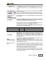
KEY TO THE SYMBOLS USED IN THIS DOCUMENT
The DANGER sign draws attention to a potential risk to a
DANGER person’s safety. All the precautions must be fully understood
and applied before proceeding.
WARNING
The WARNING sign draws attention to a potential risk of
damage to the apparatus or loss of data. All the precautions
must be fully understood and applied before proceeding.
CAUTION
The CAUTION sign draws attention against unsafe practices
for the apparatus functionality.
NOTE:
II
The NOTE draw attention to important information.
Note and symbols
Contents
Safety requirements and instructions…..........…….....…
EC Conformity Certificate…............................……………
Page
X
XI
1 General information
1.1 Documentation.......................................................……
1.2 PMM 8053B Introduction…………………………………
1.3 Standard accessories.............................................…...
1.4 Optional accessories ..............................................…..
1.5 Main specifications.................................................…...
1.6 Field probes....................................................………....
1.7 Front panel of PMM 8053B .......….................………....
1.8 Side panel of PMM 8053B …….............………………..
Page
1-1
1-1
1-1
1-1
1-2
1-3
1-40
1-40
2 Installation and use
2.1 Introduction…….......................................................…..
2.2 Preliminary inspection...........................................….....
2.3 Work environment.............................................…….....
2.4 To return for repair......................................…………....
2.5 To cleaning the meter…....................................…….....
2.6 To install and use PMM 8053B…......................…….....
2.7 RF signals of dangerous fields......................……….....
2.8 Battery charger....................................................……...
2.8.1 To substitute the mains connector…....…….........…..
2.8.2 To check the internal batteries…............................…
Page
2-1
2-1
2-1
2-1
2-1
2-2
2-2
2-2
2-2
2-3
Contents
III
3 Instructions for use
3.1 Introduction………….............................................…......
3.2 To switch on…........................................................…....
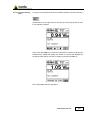
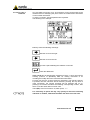
3.3 Main menu…...................................................………....
3.3.1 Data about the probe…...................................…….....
3.3.2 Status box…....................................………………......
3.3.3 Digital reading…..........................……........................
3.3.4 Analog bar….......……………………...........................
3.3.5 Main Function keys.…….............................................
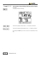
3.4 UNIT.........…….......................................................……
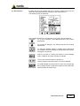
3.5 MODE............……...................................................…..
3.5.1 ABS/% Mode………….....…........................................
3.5.2 MIN-MAX/AVG – MIN-MAX/RMS ...................……….
3.5.3 PLOT Mode………………………….……………….….
3.5.4 DATA logger ……………………....…......................….
3.5.4.1 To begin storing data………………………………….
3.5.4.2 To enter a comment………......................................
3.6 To control the LCD display ……….................................
3.7 SET function…...................................…………..............
3.7.1 Alarm function….........................................………....
3.7.2 Linear average AVG or quadratic average RMS....…
3.7.3 Freq function …….............................................…..…
3.7.4 Plot function……….....................................................
3.7.5 Serial function……….................................................
3.7.6 Logger function……...................................................
3.7.6.1 Over limit……………………………………………....
3.7.6.2 Manual mode………………………………………....
3.7.6.3 Data change…………………………………………..
3.7.6.4 1s Fix…………………………………………………..
3.7.6.5 xxxs Def……………………………………………….
3.7.6.6 xxxs Def LP……………………………………………
3.7.6.7 AVG (RMS) 6 min-6………………………………….
3.7.6.8 AVG (RMS) 6 min-1………………………………….
3.7.6.9 Memory property……………………………………..
3.7.7 Log end function……...............……....................…...
3.7.8 Bar function……........................................................
3.7.9 Filter function….........................................................
3.7.10 Auto OFF function…................................................
3.7.11 Time function……....................................................
3.7.12 Date function…….....................................................
Page
3-1
3-1
3-2
3-3
3-3
3-4
3-4
3-5
3-5
3-6
3-6
3-6
3-7
3-8
3-9
3-11
3-12
3-13
3-14
3-15
3-16
3-16
3-16
3-17
3-18
3-19
3-20
3-20
3-21
3-22
3-22
3-23
3-24
3-25
3-25
3-25
3-26
3-26
3-26
4 Applications
4.1 What is electrosmog?…………....................................
4.2 Observations about the risks .......................................
4.3 Measurement of power distribution lines…………….....
4.4 Measurement of telecommunications transmitters…....
4.5 Spatial average..……........................................………..
4.6 Long-term acquisition…............................………………
4.7 dB to % error conversion………………………………….
Page
4-1
4-1
4-1
4-2
4-3
4-3
4-4
IV
Contents
5 Data transfer – 8053 Logger Interface
5.1 Introduction …………..…………………………………….
5.2 System requirements ....................................................
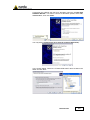
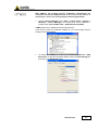
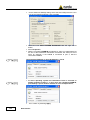
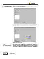
5.3 Software installation ...............................………………..
5.4 Icon of 8053 Logger Interface software ........………….
5.5 Hardware installation ...................................…………...
5.6 To run the Logger Interface software ...........…………..
5.7 To transfer data ...................................………………...
5.8 To save data ...........................................……………...
5.9 To process data with Word for WINDOWS .……………
5.10 To process data with EXCEL .....................................
Page
5-1
5-1
5-2
5-3
5-4
5-10
5-11
5-12
5-13
5-14
6 Updating Firmware
6.1 Introduction ………….……………………………………..
6.2 System requirements ........................................……….
6.3 To install the software …....................................……….
6.4 Icon of PMM 8053B software .…...................................
6.5 To install the hardware ..................................................
6.6 To run the Update software .........………………………..
6.7 To transfer data ………..................................................
Page
6-1
6-1
6-1
6-1
6-1
6-1
6-2
7 8053-SW02 Data acquisition Software
7.1 Introduction to 8053-SW02 Software ..………………….
7.2 Main specifications ..........................................…………
7.3 Software installation ……………………………..............
7.4 Commands description .……………………………...…..
7.5 Tool bar commands .……………………………………...
7.6 Graphic window .…………………………..………………
7.7 Status bar .…………………………………………………
7.8 Using SW02 with SB-04 ………………………….………
7.8.1 To use more then one SB-04 ………………….………
7.9 To use GPS module …………………………….………..
7.10 Example of using two probes without GPS ..………….
7.11 Limit activation ..………………………………………….
7.12 8053B data downloading ..………………………………
7.13 Using SW02 with 8053B ..……………………………….
7.13.1 Logger Interface …….…………………………………
7.13.2 Data acquisition …..……………………………………
7.13.3 Limit .…………………………………………..………..
Page
7-1
7-2
7-3
7-6
7-8
7-19
7-20
7-21
7-23
7-24
7-36
7-38
7-39
7-39
7-40
7-41
7-42
Contents
V
8 EHP-50C, EHP-50E Electric and Magnetic field
Analyzer
8.1 EHP-50C Introduction …………………….……………...
8.1.1 EHP-50C Main Specifications .………………………..
8.1.2 Isotropic E&H field analyzer EHP50C typical
uncertainty and anisotropy…………………………….
8.1.2.1 Typical uncertainty of EHP50C …..………………...
8.1.2.2 Explication Notes .…………………………………….
8.1.3 Anisotropy ..……………………………………………..
8.1.4 EHP-50C Panel .………………………………………...
8.1.5 Standard Accessories of PMM EHP-50C .…………..
8.1.6 Optional Accessories of PMM EHP-50C .……………
8.1.7 Installation of EHP-50C to 8053B ……………………..
8.1.8 Battery management .…………………………………..
8.1.9 EHP-50C connected to 8053B ………………………...
8.1.10 Avoiding measuring errors ..…………………………..
8.1.11 EHP-50C measuring modes ..……………..…………
8.1.12 Electric or Magnetic fields selection ...……………...
8.1.13 MODES of operations ..………………………………..
8.1.14 ABS/% mode ..………………………………………….
8.1.15 MIN-MAX/AVG-MIN-MAX/RMS modes ..……………
8.1.16 SPECT Mode ..…………………………………………
8.1.17 MARKER function in SPECT mode ..……….............
8.1.18 LOGGER function with the MARKER ..…..................
8.1.19 Data logger mode ..…………………………………….
8.1.20 Power supply - battery recharging of EHP-50C …….
8.1.21 Using EHP-50C with a UMPC or PC ..……………….
8.2 EHP-50E Introduction …………………….……………….
8.2.1 EHP-50E Main Specifications .…………………………
8.2.2 Anisotropy ..………………………………………………
8.2.3 EHP-50E Panel .………………………………………...
8.2.4 Standard Accessories of PMM EHP-50E .……………
8.2.5 Optional Accessories of PMM EHP-50E .…………….
8.2.6 Installation of EHP-50E to 8053B ……………………..
8.2.7 EHP-50E connected to 8053B ………………………...
8.2.8 Avoiding measuring errors ....………………………….
8.2.9 EHP-50E measuring modes ..……………..…………..
8.2.10 Electric or Magnetic fields selection ...……………...
8.2.11 MODES of operations ..………………………………..
8.2.12 ABS/% mode ..………………………………………….
8.2.13 MIN-MAX/AVG-MIN-MAX/RMS modes ..……………
8.2.14 SPECT Mode ..…………………………………………
8.2.15 MARKER function in SPECT mode ..……….............
8.2.16 LOGGER function with the MARKER ..…..................
8.2.17 Data logger mode ..…………………………………….
8.2.18 Power supply - battery recharging of EHP-50E …….
8.2.19 Using EHP-50E with a UMPC or PC ..……………….
VI
Contents
Page
8-1
8-2
8-3
8-3
8-4
8-5
8-6
8-6
8-6
8-7
8-8
8-9
8-10
8-11
8-12
8-12
8-12
8-13
8-13
8-15
8-15
8-16
8-16
8-17
8-18
8-19
8-20
8-21
8-21
8-21
8-22
8-23
8-24
8-25
8-26
8-26
8-26
8-27
8-27
8-29
8-29
8-30
8-30
8-31
9 EHP-200A Electric and Magnetic field analyzer
9.1 Introduction……………………….………………………..
9.2 EHP-200A Main specification…..………………………..
9.3 EHP-200A Main specification with 8053B………….…..
9.4 EHP-200A Panel….…….………………………………...
9.5 EHP-200A Standard accessories…..………….……..…
9.6 EHP-200A Optional accessories.……………...……..…
9.7 Installation of EHP-200A …………………………..…….
9.8 EHP-200A connected to 8053B….………………....…..
9.9 Avoiding measurements errors…………………..….….
9.10 Main menù…………………………………….…………
9.11 To control the LCD display…...………………….…….
9.12 SET function……………………………………….…….
9.13 Electric or Magnetic fields selection……………..……
9.14 MODES of operation……………………………………
9.15 ABS% mode…….....................................…………….
9.16 MIN-MAX/AVG e MIN-MAX/RMS modes.……………
9.17 FULL SPAN mode………………………………………
9.18 Data Logger mode………………………………………
9.19 Power supply and battery recharging of EHP-200A….
9.20 Using EHP-200A with a UMPC or Personal computer.
Page
9-1
9-2
9-3
9-4
9-4
9-4
9-5
9-6
9-7
9-8
9-8
9-8
9-9
9-9
9-9
9-9
9-9
9-10
9-11
9-12
10 EP600/EP601/EP602 Electric field probe
10.1 Introduction………………………………………………
10.2 Specifications EP600…………………………………...
10.3 Frequency Response for EP600 ..…………………….
10.4 Specifications EP601……………………………………
10.5 Frequency Response for EP601 ..…………………….
10.6 Specifications EP602 ……………………………………
10.7 Frequency Response for EP602 ……………………….
10.8 Housing and connectors ……………………………….
10.9 Standard accessories…………………………………..
10.10 Options…………………………………………………...
10.11 EP600/EP601/EP602 connected to 8053B …………
10.12 Preventing measurement errors……………………...
10.13 Connection of fiber optic extension FO-EP600/10…
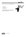
10.14 EP600/EP601/EP602 installation on the conical
holder ……………………………………………………
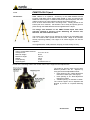
10.15 EP600/EP601/EP602 installation on tripod
PMM TR-02 …………………………………………….
10.16 EP600 CHARGER……………………………………..
10.17 EP600/EP601/EP602 with 8053B ..………………….
10.17.1 Operational modes………………………………..…
10.17.2 Preliminary operations………………………………
10.17.3 Display of the values of the field……………………
10.17.3.1 ABS/% mode……………………………………….
10.17.3.2 MIN-MAX/AVG and MIN-MAX/RMS……………..
10.17.4 Graph display data…………………………………...
10.17.4.1 PLOT mode…………………………………………
10.17.5 Store and display data……………………………….
10.18 Operating PMM EP600/EP601/EP602 with PC ……..
Page
10-1
10-2
10-3
10-4
10-5
10-6
10-7
10-8
10-8
10-8
10-9
10-11
10-12
10-13
10-14
10-15
10-18
10-18
10-19
10-20
10-20
10-20
10-21
10-21
10-21
10-22
Contents
VII
11 Accessories
11.1 Introduction…………………………………….…………
11.2 Preliminary inspection………………………….……….
11.3 Work environment……………………………….……...
11.4 Return for repair…………………………………..……..
11.5 Cleaning……………………………………………..……
11.6 Power supply and battery chargers………………..…..
11.7 OR-03 Optical Repeater………....................…..……..
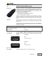
11.8 USB-OC Optical USB Converter……………………....
11.9 8053-OC Optical Converter..................……...….…….
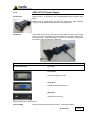
11.10 8053-OC-PS Power Supply…………………………...
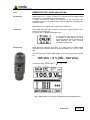
11.11 8053-Cal Calibration Probe.......................…..……...
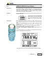
11.12 8053-ZERO Zeroing Calibrator...........….......…........
11.13 8053-RT Trigger………......................……….....…...
11.14 TR-02A Tripod………………………….............……..
11.15 TT-01 Fiber Glass Telescopic Support………………
11.16 8053-GPS Global Positioning System……….……...
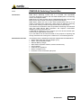
11.17 SB-04 Switching Control Box…...............……….…..
11.18 Other accessories………………………………….…..
Page
11-1
11-1
11-1
11-1
11-1
11-2
11-3
11-7
11-9
11-11
11-13
11-15
11-17
11-19
11-21
11-23
11-31
11-37
12 Measuring electromagnetic fields
12.1 Introduction.............................................................…
12.1.1 Quantities to be considered.....................................
12.2 Dosimetric measurements..........................................
12.3 Exposure measurements...........................................
12.4 Characteristics of the sources....................................
12.5 Measurement apparatus.........................................…
12.6 General requirements.................................................
12.7 Probes.........…........................................................…
12.8 Cables.......…..........................................................…
12.9 Measurement units.....................................................
12.10 Broad band apparatus………………………………..
12.11 Narrow band apparatus….................…...................
12.12 Type of apparatus ……….............…........................
12.13 Diode apparatus............….......................................
12.13.1 Spurious responses.....…......................................
12.14 Bolometric apparatus…............…............................
12.15 Thermocouple apparatus.....…................................
12.16 Spurious responses due to the apparatus...............
12.16.1 Cable coupling…………..................…..................
12.16.2 Thermoelectric effect on coupling cables…….....
12.16.3 Coupling between the probe and conductors.......
12.16.4 Static fields....….….............................................…
12.16.5 Outside bandwidth responses..............................
12.16.6 Calibration of the apparatus….......................…...
12.17 Measurement procedures…….................................
12.17.1 Preliminaries..........................................................
12.17.2 Near fields and far fields…...........................……..
12.17.3 Operational tests of the measurement apparatus...
12.17.4 Disturbed fields.......................................................
12.18 Measurement of far fields...................................……
12.18.1 Initial measurements.............................................
12.18.2 Multiple sources.....................................................
12.18.3 Near radiative fields..........................................….
12.18.4 Presentation of results….......................................
Page
12-1
12-1
12-1
12-1
12-1
12-1
12-2
12-2
12-2
12-2
12-2
12-2
12-2
12-3
12-3
12-4
12-4
12-4
12-4
12-4
12-4
12-5
12-5
12-5
12-5
12-5
12-6
12-6
12-6
12-6
12-7
12-7
12-7
12-7
13 8053B programming commands
13.1 Introduction………………………………………..…..
13.2 List of commands……………………………..………
Page
13-1
13-2
VIII
Contents
Figures
Figure
1-1
1-2
5-1
5-2
8-1
8-2
8-3
8-4
9-1
10-1
10-2
10-3
10-4
10-5
10-6
10-7
10-8
10-9
10-10
10-11
10-12
10-13
10-14
11-1
11-2
11-3
11-4
11-5
11-6
11-7
11-8
11-9
11-10
11-11
11-12
Page
8053B Front panel .....………...............……………….....................
8053B Side panel .…….......…..............……………………………..
8053B link with USB-OC …………….………………………………..
8053B link with 8053-OC ….………………………………………….
EHP-50C Block diagram …............................................................
3D mesh measurements of magnetic probe .……….....................
EHP-50C Panel .................……….....………………………………..
EHP-50E Panel .................……….....………………………………..
EHP-200A Panel …….…………………………………………………
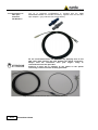
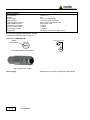
EP600/EP601/EP602 ………………………………………………….
EP600 Frequency Response ..……………………………………….
EP601 Frequency Response ..………………………………………..
EP602 Frequency Response ..………………………………………..
Plastic housing .………………………………………………………..
Optical connectors .…………………………………………………….
EP600/EP601/EP602 with FO-EP600/10 extension ……………….
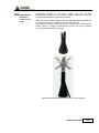
EP600/EP601/EP602 mounted on conical holder ….....................
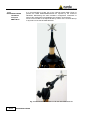
EP600/EP601/EP602 on TR-02A ……………………………………
EP600/EP601/EP602 on TR-02A with PMM 8053-SN ……………
AC adapter ……………………………………………………………..
EP600 CHARGER……………………………………………………..
EP600 CHARGER components………………………………………
EP600/EP601/EP602 on EP600 CHARGER ..……………………..
OR-03 Panel……………….……...................…..............................
USB-OC Adapters……………………..………………......................
8053-OC Panel….……..…...............………………….....................
8053-OC-PS Connector………………………………………………..
8053-CAL Connector……………………….....………......................
8053-ZERO Zeroing Calibrator......................……………………….
8053-RT Connector….......................……....…..............................
TR-02A Tripod………………………..........……..............................
TT-01 Fiber Glass Telescopic Support………………………………
8053-GPS Panel...............................……......………………………
SB-04 Front panel……………………………...………………………
SB-04 Rear panel….………………...…………………………………
1-40
1-40
5-4
5-4
8-1
8-5
8-6
8-21
9-4
10-1
10-3
10-5
10-7
10-8
10-8
10-12
10-13
10-14
10-14
10-15
10-15
10-16
10-17
11-5
11-7
11-9
11-11
11-13
11-15
11-18
11-19
11-21
11-25
11-33
11-33
Contents
IX
Tables
Table
1-1
1-2
7-1
8-1
8-2
9-1
9-2
10-1
10-2
10-3
10-4
10-5
11-1
11-2
11-3
11-4
11-5
11-6
11-7
11-8
11-9
11-10
11-11
X
Technical Specifications of the 8053B ………………………
Technical Specifications of the Field probes ......................
8053-SW02 Requirements and specifications....................
Technical Specifications of EHP-50C..................................
Technical Specifications of EHP-50E..................................
Technical Specifications of EHP-200A Field Analyzer……..
Technical Specifications of EHP-200A Selective probe…...
Specifications of the electric field probe EP600…………….
Specifications of the electric field probe EP601…………….
Specifications of the electric field probe EP602…………….
EP600 CHARGER Led status - Start up phase ……….….
EP600 CHARGER Led status - Charger phase …….........
Technical Specifications of OR-03..........……………………
Technical Specifications of USB-OC...................................
Technical Specifications of 8053-OC..................................
Technical Specifications of 8053-OC-PS............................
Technical Specifications of 8053-CAL.................................
Technical Specification of 8053-ZERO...............................
Technical Specification of 8053-RT…………......................
Technical Specifications of TR-02A.........…........................
Technical Specifications of TT-01............…........................
Technical Specifications of 8053-GPS.................................
Technical Specifications of SB-04.........…...........................
Contents
Page
1-2
1-4
7-2
8-2
8-19
9-2
9-3
10-2
10-4
10-6
10-17
10-17
11-3
11-7
11-9
11-11
11-14
11-16
11-18
11-19
11-21
11-24
11-32
SAFETY RECOMMENDATIONS AND INSTRUCTIONS
This product has been designed, produced and tested in Italy, and it left the factory in conditions fully
complying with the current safety standards. To maintain it in safe conditions and ensure correct use,
these general instructions must be fully understood and applied before the product is used.
• When the device must be connected permanently, first provide effective grounding;
• If the device must be connected to other equipment or accessories, make sure they are all safely
grounded;
• In case of devices permanently connected to the power supply, and lacking any fuses or other
devices of mains protection, the power line must be equipped with adequate protection
commensurate to the consumption of all the devices connected to it;
• In case of connection of the device to the power mains, make sure before connection that the voltage
selected on the voltage switch and the fuses are adequate for the voltage of the actual mains;
• Devices in Safety Class I, equipped with connection to the power mains by means of cord and plug,
can only be plugged into a socket equipped with a ground wire;
• Any interruption or loosening of the ground wire or of a connecting power cable, inside or outside the
device, will cause a potential risk for the safety of the personnel;
• Ground connections must not be interrupted intentionally;
• To prevent the possible danger of electrocution, do not remove any covers, panels or guards installed
on the device, and refer only to NARDA Service Centers if maintenance should be necessary;
• To maintain adequate protection from fire hazards, replace fuses only with others of the same type
and rating;
• Follow the safety regulations and any additional instructions in this manual to prevent accidents and
damages.
Safety considerations
XI
EC Conformity Certificate
(in accordance with the ISO/IEC standard 17050-1 and 17050-2)
This is to certify that the product: PMM 8053B Portable Field Meter
Produced by: Narda Safety Test Solutions
Via Benessea 29/B
17035 Cisano sul Neva (SV) – ITALY
complies with the following European Standards:
Safety: CEI EN 61010-1 (2001)
EMC: EN 61326-1 (2007)
This product complies with the requirements of Low Voltage Directive 2006/95/CE and with EMC
Directive 2004/108/CE.
Narda Safety Test Solutions
XII
EC Conformity
1 – General information
1.1 Documentation
The following Appendices are included in this Manual:
• A questionnaire to be sent to NARDA together with the apparatus
should service be required.
• A checklist of the Accessories included in the shipment.
This Manual includes the description of the Accessories of the system for
the measurement of electromagnetic fields.
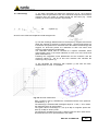
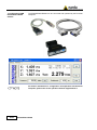
1.2 PMM 8053B
Introduction
PMM 8053B is a versatile and expandable test system suitable for
measuring electric and magnetic fields relating to electrosmog.
The system consists of various electric and magnetic field probes and of a
compact and portable meter equipped with a wide LCD display, 4 simple
function keys (which allow different actions and settings, in accordance with
the selected menu), internal rechargeable batteries and RS232 and fiber
optic interfaces. The system also has a wide range of Accessories, which
have been designed for all the needs of the tests.
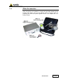
1.3 Standard accessories The standard accessories included with PMM 8053B are:
• Soft Carrying Case;
• Serial Cable (1.5m long);
• USB-RS232 Converter
• Battery Charger;
• Downloading & firmware update Program Disk;
• 8053-SW02 Data acquisition software
• User’s Manual;
• Calibration Certificate;
• Return for Repair Form.
1.4 Optional accessories
The following accessories may be ordered separately:
•
•
•
•
•
•
•
•
•
•
•
•
•
•
•
•
•
•
•
•
•
FO-8053/10 Fiber Optic Cable (10m);
FO-8053/20 Fiber Optic Cable (20m);
FO-8053/40 Fiber Optic Cable (40m);
FO-8053/80 Fiber Optic Cable (80m);
FO-10USB Fiber Optic Cable (10m);
FO-20USB Fiber Optic Cable (20m);
FO-40USB Fiber Optic Cable (40m);
TT-01 Fiber Glass Telescopic Support;
TR-02A Tripod with Swivel;
OR-03 Programmable Optical Repeater;
SB-04 Switching Control Box;
8053-CC Rigid Carrying Case;
8053-CA Car Adapter;
8053-BC Additional Battery Charger;
8053-OC Optical Converter;
8053-OC-PS Power Supply
USB-OC Optical Converter;
8053-GPS GPS Unit;
8053-RT Remote Trigger;
8053-CAL Calibration Probe;
8053-ZERO Zeroing Calibrator for 8053.
Document 8053BEN-40918-3.16 - © NARDA 2014
General information
1-1
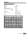
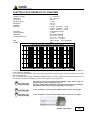
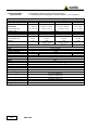
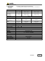
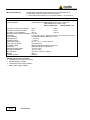
Table 1-1 lists the specifications of PMM 8053B. The specifications of all
accessories are listed in the Chapter on Accessories.
The following conditions apply to all specifications:
• Temperature for use must be between -10°C and +40°C.
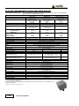
TABLE 1-1 – Technical Specifications of PMM 8053B General Purpose Field Meter
Frequency Range
Frequency range
1 Hz - 40 GHz (depending on the probe)
Dynamic range
>140 dB (depending on the probe)
Operating range
|
Resolution
| Depending on the probe (See Table 1-2)
Sensitivity
|
Units
V/m, kV/m, µW/cm², mW/cm², W/m², A/m, nT, µT, mT;
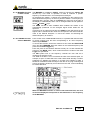
LCD Display
Field measured
X, Y, Z in absolute values, percent and total.
Time
Internal clock in real time
Probe
Display of the model and date of calibration
Graphic bar
The analog bar displays:
- real time value with respect to full scale;
- field versus time (in linear or logarithmic form) with automatic time scaling;
- alarm threshold.
Measuring function
Time of complete
150 ms with 80 Hz filter
acquisition
250 ms with 40 Hz filter
450 ms with 20 Hz filter
(Total time for 3 axes)
900 ms with 10 Hz filter
Internal memory
Up to 32.700 measurements (up to 8.100 standard memory, up to 21.600
extended memory)
Alarm
Variable threshold from 0 to 100% of full scale. Internal sound with blinking
symbol on the display and output signal on RS-232 connectors when the
level is greater than the alarm threshold
Functions
Minimum, Maximum and Averaging
Averaging mode
Arithmetic, quadratic (RMS), manual, rolling and spatial
Averaging time
Definable 30 sec, 1, 2, 3, 6,10,15, 30 min or manual
Data acquisition
Sampling mode (1, 10-900 sec/sample), data change, over the limit,
(Logger)
average on 6 min, manual, spectrum (with EHP-50C)
General specifications
Output
LCD display 72x72mm 128x128 pixel, RS232 (with cable or fiber optic)
Input
Direct through Fischer connector or via fiber optic connector
Internal battery
Rechargeable at NiMH (5 x 1.2 V)
Operational time
24 hours normal mode, 48 hours (in SAVE MODE function: display off)
Recharge time
< 4 hours (15 minutes charge for 1 hour of use)
External power supply
DC, 10 - 15 V, I = about 500 mA
Interfaces
RS232 (remote control, calibration and firmware update)
Software/Firmware
Upgrade available via Internet at the Web site: www.narda-sts.it
Autotest
Automatic during switch-on of all functions; automatically checks every
individual diode
Calibration
Inside the built-in E²PROM of the probe
Conformity
With Directives 89/336 and 73/23 and the amendments to them
CEI 211-6 and 211-7
Operating temperature
From -10 to +40°C
Storage temperature
From -20 to +70°C
Size (WxHxD)
108 x 240 x 50 mm
Weight
1.07 kg
Tripod support
Threaded insert ¼”
1.5 Main specifications
1-2
General information
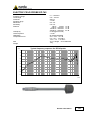
PMM 8053B measurement system is complete with a series of electric and
magnetic field probes in the frequency range from 5 Hz to 40 GHz.
1.6 Field probes
Field Probes
Frequency range
Level range
Electric Field Probe EP-105
100 kHz - 1000 MHz
0.05 - 50 V/m
Electric Field Probe EP-300
100 kHz - 3 GHz
0.1 - 300 V/m
Electric Field Probe EP-330
100 kHz - 3 GHz
0.3 - 300 V/m
Electric Field Probe EP-301
100 kHz - 3 GHz
1 - 1000 V/m
Electric Field Probe EP-333
100 kHz – 3.6 GHz
0.15 - 300 V/m
Electric Field Probe EP-183
1 MHz – 18 GHz
0.8 - 800 V/m
Electric Field Probe EP-408
1 MHz – 40 GHz
0.8 - 800 V/m
Electric Field Probe EP-44M
100 kHz - 800 MHz
0.25 - 250 V/m
Electric Field Probe EP-33M
700 MHz - 3 GHz
0.3 - 300 V/m
Electric Field Probe EP-33A
925 MHz - 960 MHz
0.03 - 30 V/m
Electric Field Probe EP-33B
1805 MHz - 1880 MHz
0.03 - 30 V/m
Electric Field Probe EP-33C
2110 MHz - 2170 MHz
0.03 - 30 V/m
Electric Field Probe EP-201
60 MHz – 12 GHz
3 – 500 V/m
Electric Field Probe EP-600
100 kHz – 9.25 GHz
0.14 – 140 V/m
Electric Field Probe EP-601
10 kHz – 9.25 GHz
0.5 – 500 V/m
Electric Field Probe EP-602
5 kHz – 9.25 GHz
1.5 – 1500 V/m
Electric Field Probe EP-645
100 kHz – 6.5 GHz
0.35 – 450 V/m
Electric Field Probe EP-745
100 kHz – 7 GHz
0.35 – 450 V/m
Magnetic Field Probe HP-032
0.1 - 30 MHz
0.01 - 20 A/m
Magnetic Field Probe HP-102
30 - 1000 MHz
0.01 - 20 A/m
Magnetic Field Probe HP-050
10 Hz – 5 kHz
10 nT – 40 µT
Magnetic Field Probe HP-051
10 Hz – 5 kHz
50 nT – 200 µT
Electric and Magnetic Field Analyzers EHP-50C
5 Hz – 100 kHz
10 mV/m – 100 kV/m
1 nT – 10 mT
Electric and Magnetic Field Analyzers EHP-50E
1 Hz – 400 kHz
5 mV/m – 100 kV/m
0.3 nT – 10 mT
Electric and Magnetic Field Analyzers EHP-200A
9 kHz – 30 MHz (*)
0.1 V/m – 1000 V/m
3 mA/m – 300 A/m (*)
(*) The values depends on the setting of the magnetic field. See EHP200A specifications.
General information
1-3
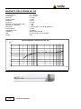
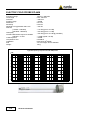
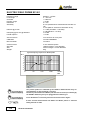
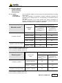
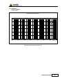
TABLE 1-2 Technical Specifications of the Field Probes
ELECTRIC FIELD PROBE EP-330
Frequency range
Level range
Overload
Dynamic range
Resolution
Sensitivity
Absolute error @ 50 MHz 20 V/m
Flatness (10 - 300 MHz)
Flatness (3 MHz - 3 GHz)
Isotropicity
H-field rejection
Temperature error
Calibration
Size
Weight
[dB]
100 kHz - 3 GHz
0.3 - 300 V/m
> 600 V/m
> 60 dB
0.01 V/m
0.3 V/m
± 0.8 dB
± 0.5 dB
± 1.5 dB
± 0.8 dB (typical ± 0.5 dB @ 930 and 1800 MHz)
>20 dB
20°C ÷ 60°C = ±0.1 dB
0°C ÷ 20°C = -0.05 dB/°C
-20°C ÷ 0°C = -0.15 dB/°C
2
Internal into E PROM
317 mm length, 58 mm diameter
100 g
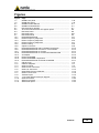
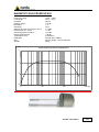
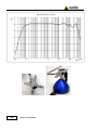
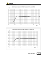
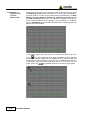
Typical frequency response for EP-330 probe
@20V/m
1.0
0.0
-1.0
-2.0
-3.0
-4.0
-5.0
-6.0
0.1
1-4
1
General information
10
100
1000
10000
[MHz]
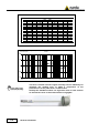
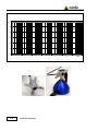
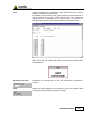
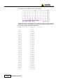
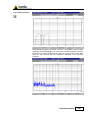
Typical response for signal GSM, 1 frequency channel, 1 time slot
Correction factor
EP330
2.00
1.50
1.00
0.50
0.00
1
10
100
300
Erms [V/m]
Erms [V/m]
1
2
3
4
5
6
7
8
9
10
20
30
40
50
60
70
80
90
100
200
300
Edisplay [V/m]
0.98
1.91
2.82
3.70
4.58
5.40
6.17
6.96
7.75
8.50
15.84
21.3
28.6
38.5
51.3
62.5
75.1
88.1
99
227
361
Correction factor
1.02
1.05
1.06
1.08
1.09
1.11
1.13
1.15
1.16
1.18
1.26
1.41
1.40
1.30
1.17
1.12
1.07
1.02
1.01
0.88
0.83
This test is carried out with a signal currently used in laboratory for
maximize the reading error to make a comparison of the
performances of the probe with a common base.
Actually the radiobase station use eight time slots of each channel
so the effective error of the measurement is negligible.
General information
1-5
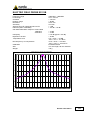
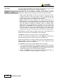
EP330 - Typical amplitude response for two CW signal of same level. (Fc=1MHz)
Erms/Edisplay
d f= 1kHz
df = 10kHz
df = 100kHz
df = 1MHz
1.600
1.400
1.200
1.000
0.800
0.600
0.400
0.1
1-6
1
General information
10
100
1000
Erms[V/m]
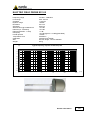
ELECTRIC FIELD PROBE EP-33M
Frequency range
Level range
Overload
Dynamic range
Resolution
Sensitivity
Absolute error @ 930 MHz 20 V/m
Flatness (900 MHz - 3 GHz)
Isotropicity
H-field rejection
Temperature error
Calibration
Size
Weight
[dB]
700 MHz - 3 GHz
0.3 - 300 V/m
> 600 V/m
> 60 dB
0.01 V/m
0.3 V/m
± 1 dB
± 1.5 dB
± 0.8 dB (typical ± 0.5 dB @ 930 and 1800 MHz)
> 20 dB
0.05 dB/°C
2
Internal into E PROM
317 mm length, 58 mm diameter
100 g
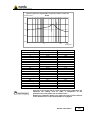
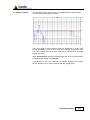
Typical frequency response for EP-33M probe
5
0
-5
-10
-15
-20
-25
100
10000[MHz]
1000
General information
1-7
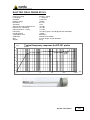
MAGNETIC FIELD PROBE HP-102
Frequency range
Level range
Overload
Dynamic range
Resolution
Sensitivity
Absolute error @ 50 MHz 2 A/m
Flatness (50 - 900 MHz)
Isotropicity
E-field rejection
Temperature error
Calibration
Size
Weight
30 - 1000 MHz
0.01 - 20 A/m
> 40 A/m
> 60 dB
1 mA/m
0.01 A/m
± 1 dB
± 1 dB
± 0.8 dB (typical ± 0.5 dB @ 930 MHz)
> 20 dB
0.05 dB/°C
2
Internal into E PROM
317 mm length, 58 mm diameter
110 g
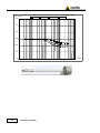
Typical frequency response for HP-102
[dB]
4
2
0
-2
-4
-6
10
1-8
100
General information
1000
[MHz]
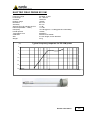
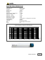
ELECTRIC FIELD PROBE EP-105
Frequency range
Level range
Overload
Dynamic range
Resolution
Sensitivity
Absolute error @ 50 MHz 6 V/m
Flatness (10 - 300 MHz)
Flatness (300 kHz - 1 GHz)
Isotropicity
H-field rejection
Temperature error
Calibration
Size
Weight
100 kHz - 1000 MHz
0.05 - 50 V/m
> 100 V/m
> 60 dB
0.01 V/m
0.05 V/m
± 0.8 dB
± 0.5 dB
± 1 dB
± 0.8 dB (typical ± 0.5 dB @ 930 MHz)
> 20 dB
0.05 dB/°C
2
Internal into E PROM
350 mm length, 133 mm diameter
290 g
Typical frequency response for EP-105 probe
[dB]
1,0
0,0
-1,0
-2,0
-3,0
-4,0
-5,0
-6,0
-7,0
-8,0
0,1
1
10
100
1000
General information
10000
[MHz]
1-9
MAGNETIC FIELD PROBE HP-032
Frequency range
Level range
Overload
Dynamic range
Resolution
Sensitivity
Absolute error @ 1 MHz 2 A/m
Flatness (1 -25 MHz)
Isotropicity
E-field rejection
Temperature error
Calibration
Size
Weight
0.1 - 30 MHz
0.01 - 20 A/m
> 40 A/m
> 60 dB
1 mA/m
0.01 A/m
± 1 dB
± 1 dB
± 0.8 dB (typical ± 0.5 dB @ 1 MHz)
> 20 dB
0.05 dB/°C
2
Internal into E PROM
350 mm length, 133 mm diameter
400 g
Typical frequency response for HP-032 probe
[dB]
5
4
3
2
1
0
-1
-2
-3
-4
-5
-6
-7
-8
-9
-10
0.01
1-10
0.1
General information
1
10
100 [MHz]
ELECTRIC FIELD PROBE EP-301
Frequency range
Level range
Overload
Dynamic range
Resolution
Sensitivity
Absolute error @ 50 MHz 20 V/m
Flatness (10 - 300 MHz)
Flatness (3 MHz - 1 GHz)
Isotropicity
H-field rejection
Temperature error
Calibration
Size
Weight
[dB]
100 kHz - 3 GHz
1 – 1000 V/m
> 1200 V/m
> 60 dB
0.1 V/m
1 V/m
± 0.8 dB
± 0.5 dB
± 1.5 dB
± 0.8 dB (Typical ± 0.5 dB @ 930 and 1800 MHz)
> 20 dB
0.05 dB/°C
2
Internal into E PROM
317 mm length, 58 mm diameter
100 g
Typical frequency response for EP-301 probe
@20V/m
1.0
0.0
-1.0
-2.0
-3.0
-4.0
-5.0
-6.0
0.1
1
10
100
1000
General information
10000
[MHz]
1-11
ELECTRIC FIELD PROBE EP-183
Frequency range
Level range
Overload
Dynamic range
Resolution
Sensitivity
Absolute error @ 200 MHz 6 V/m
Flatness (1 MHz - 1 GHz)
Flatness (1 - 3 GHz)
Flatness (3 - 18 GHz)
Isotropicity @ 200 MHz
H-field rejection
Temperature error
Calibration
Size
Weight
1 MHz - 18 GHz
0.8 - 800 V/m
> 1200 V/m
> 60 dB
0.01 V/m
0.8 V/m
± 0.8 dB
± 1.5 dB
± 2.0 dB
± 2.5 dB
± 0.8 dB (typical ± 0.5 dB @ 930 and 1800 MHz)
> 20 dB
0.02 dB/°C
2
Internal into E PROM
317 mm length, 50 mm diameter
90 g
Typical frequency response for EP-183 probe
[dB]
2
1
0
-1
-2
-3
-4
-5
-6
-7
-8
-9
-10
0.1
1-12
1
10
General information
100
1000
10000
[MHz]
100000
ELECTRIC FIELD PROBE EP-408
Frequency range
Level range
Overload
Dynamic range
Resolution
Sensitivity
Absolute error @ 200 MHz 6 V/m
Flatness (1 MHz - 1 GHz)
Flatness (1 - 3 GHz)
Flatness (3 - 18 GHz)
Flatness (18 - 26.5 GHz)
Flatness (26.5 - 40 GHz)
Isotropicity @ 200 MHz
H-field rejection
Temperature error
Calibration
Size
Weight
1 MHz - 40 GHz
0.8 - 800 V/m
> 1000 V/m
> 60 dB
0.01 V/m
0.8 V/m
± 0.8 dB
± 1.5 dB
± 2 dB
± 2.5 dB
± 3 dB
± 4 dB
± 0.8 dB (typical ± 0.5 dB @ 930 and 1800 MHz)
> 20 dB
0.02 dB/°C
2
internal into E PROM
317 mm length, 52 mm diameter
90 g
Typical frequency response for EP-408 probe
[dB]
5
3
1
-1
-3
-5
-7
-9
-11
-13
-15
0,1
1
10
100
1000
10000
General information
[MHz]
100000
1-13
ELECTRIC FIELD PROBE EP-44M
Frequency range
Level range
Overload
Dynamic range
Resolution
Sensitivity
Absolute error @ 50 MHz and 6 V/m
Flatness
(10 MHz - 200 MHz)
(200 MHz - 800 MHz)
Isotropicity
Out band attenuation respect to 50 MHz
900 MHz – 3 GHz
H-field rejection
Temperature error
Calibration
Size
Weight
100 kHz - 800 MHz
0.25 - 250 V/m
> 500 V/m
> 60 dB
0.01 V/m
0.25 V/m
± 0.8 dB
± 1.5 dB (typical ± 0.8 dB)
± 2.0 dB (typical ± 1.5 dB)
± 0.8 dB (typical ± 0.5 dB @ 740 MHz)
> 12 dB (typical >15 dB)
> 20 dB
0.02 dB/°C
2
Internal into E PROM
317 mm length, 58 mm diameter
100 g
Typical frequency response for EP-44M probe
[dB]
10
5
0
-5
-10
-15
-20
-25
-30
0.1
1-14
1
General information
10
100
1000
[MHz] 10000
MAGNETIC FIELD PROBE HP-050
Frequency range
Level range
Overload
Dynamic range
Resolution
Sensitivity
Absolute error @ 50 Hz 200 nT 25 °C
Flatness (40 Hz – 1kHz)
Isotropicity @ 50 Hz 200 nT
Electric field rejection
Temperature error
Calibration
Size
Weight
[dB]
10 Hz – 5 kHz
10 nT – 40 µT
400 µT
> 72 dB
1 nT
10 nT
± 0.4 dB
± 1 dB
± 0.3 dB
> 20 dB
0.015 dB/°C
2
Internal into E PROM
350 mm length, 133 mm diameter
400 g
Tipical frequency response for HP050 probe
5
0
-5
-10
10
100
1000
General information
10000 [Hz]
1-15
ELECTRIC FIELD PROBE EP-300
Frequency range
Level range
Overload
Dynamic range
Resolution
Sensitivity
Absolute error @ 50 MHz 20 V/m
Flatness (10 - 300 MHz)
Flatness (3 MHz - 3 GHz)
Isotropicity
H-field rejection
100 kHz - 3 GHz
0.1 - 300 V/m
> 600 V/m
> 66 dB (typical >70 dB)
0.01 V/m
0.15 V/m (typical >0.1V/m)
± 0.8 dB
± 0.5 dB
± 1.5 dB
± 0.8 dB (typical ± 0.5 dB @ 930 and 1800 MHz)
>20 dB
20°C ÷ 60°C = ± 0.1 dB
0°C ÷ 20°C = -0.05 dB/°C
-20°C ÷ 0°C = -0.15 dB/°C
2
Internal into E PROM
317 mm length, 58 mm diameter
100 g
Temperature error
Calibration
Size
Weight
[dB]
Typical frequency response for EP-300 probe
@20V/m
1.0
0.0
-1.0
-2.0
-3.0
-4.0
-5.0
-6.0
0.1
1-16
1
General information
10
100
1000
10000
[MHz]
ELECTRIC FIELD PROBE EP-33A
Frequency range
Level range
Overload
Dynamic range
Resolution
Sensitivity
Absolute error @ 942.5 MHz and 2 V/m
Flatness (925 - 960 MHz)
OFF Band attenuation respect to 942.5 MHz
860 MHz
1025 MHz
Isotropicity
Rejection to H field
Temperature error
925 MHz - 960 MHz
0.03 – 30 V/m
> 120 V/m
> 60 dB
0.001 V/m
0.03 V/m
± 1 dB
+ 0.2 dB / -1.8 dB
> 10 dB
> 10 dB
± 0.8 dB (typical ± 0.5 dB)
> 20 dB
0°C ÷ 60°C = ± 0.2 dB
-20°C ÷ 0°C = -0.1 dB/°C
40°C ÷ 60°C = ± 100 kHz
-20°C ÷ 40°C = -100 kHz/°C
2
E PROM internal
317 mm length, 58 mm diameter
100 g
Drift Frequency Vs Temperature
Calibration
Size
Weight
Typical frequency response for EP33A probe
[dB]
0
-5
-10
-15
-20
-25
-30
-35
-40
0
188,5
377
565,5
754
942,5
1131
1319,5
1508
1696,5
1885
[MHz]
General information
1-17
Typical frequency response for EP33A probe
[dB]
0,0
-5,0
-10,0
-15,0
855
872,5
890
907,5
925
942,5
960
977,5
995
1012,5
1030
[MHz]
Correction factor
Typical amplitude response for a GSM, 1 frequency channel,1 time slot
EP33A
2,00
1,50
1,00
0,50
0,00
0,01
0,1
1
10
100
Erms [V/m]
This test is carried out with a signal currently used in laboratory for
maximize the reading error to make a comparison of the
performances of the probe with a common base.
Actually the radiobase station use eight time slots of each channel
so the effective error of the measurement is negligible.
1-18
General information
ELECTRIC FIELD PROBE EP-33B
Frequency range
Level range
Overload
Dynamic range
Resolution
Sensitivity
Absolute error @ 1842.5 MHz and 2 V/m
Flatness (1805 - 1880 MHz)
OFF Band attenuation respect to 1842.5 MHz
1580 MHz
2010 MHz
Isotropicity
Rejection to H field
Temperature error
Drift Frequency Vs Temperature
Calibration
Size
Weight
1805 MHz – 1880 MHz
0.03 – 30 V/m
> 120 V/m
> 60 dB
0.001 V/m
0.03 V/m
± 1 dB
+ 0.2 dB / -1.8 dB
> 10 dB
> 10 dB
± 0.8 dB (typical ± 0.5 dB)
> 20 dB
0°C ÷ 60°C = ± 0.2dB
-20°C ÷ 0°C = -0.1 dB/°C
40°C ÷ 60°C = ± 100 kHz
-20°C ÷ 40°C = -100 kHz/°C
2
E PROM internal
317 mm length, 58 mm diameter
100 g
Typical frequency response for EP33B probe
0
-5
-10
-15
-20
-25
-30
921.3
1105.6
1289.8
1474.1
1658.3
1842.6
2026.8
2211.1
2395.3
2579.6
2763.8
General information
1-19
Typical frequency response for EP33B probe
0
-1
-2
-3
-4
-5
-6
-7
-8
-9
-10
1730.0
1-20
1767.5
General information
1805.0
1842.5
1880.0
1917.5
1955.0
ELECTRIC FIELD PROBE EP-33C
Frequency range
Level range
Overload
Dynamic range
Resolution
Sensitivity
Absolute error @ 2140 MHz and 2 V/m
Flatness (2110 - 2170 MHz)
OFF Band attenuation respect to 2140 MHz
1880 MHz
2320 MHz
Isotropicity
Rejection to H field
Temperature error
Drift Frequency Vs Temperature
Calibration
Size
Weight
2110 MHz – 2170 MHz
0.03 – 30 V/m
> 120 V/m
> 60 dB
0.001 V/m
0.03 V/m
± 1 dB
+ 0.2 dB / -1.8 dB
> 10 dB
> 10 dB
± 0.8 dB (typical ± 0.5 dB)
> 20 dB
0°C ÷ 60°C = ± 0.2dB
-20°C ÷ 0°C = -0.1 dB/°C
40°C ÷ 60°C = ± 100 kHz
-20°C ÷ 40°C = -100 kHz/°C
2
E PROM internal
317 mm length, 58 mm diameter
100 g
Typical frequency response for EP33C probe
[dB]
0
-2
-4
-6
-8
-10
-12
-14
-16
-18
-20
1679.4
1863.6
2047.9
2232.1
2416.4
[MHz]
General information
1-21
Typical frequency response for EP33C probe
[d B]
0
-1
-2
-3
-4
-5
-6
-7
-8
-9
-10
2065.0
2080.0
2095.0
2110.0
2125.0
2140.0
2155.0
2170.0
2185.0
2200.0
2215.0
[M Hz]
1-22
General information
MAGNETIC FIELD PROBE HP-051
Frequency range
Level range
Dynamic range
Overload
Resolution
Sensitivity
Absolute error @ 50 Hz - 3 µT - 25°C
Flatness @ 40 Hz – 1 KHz
Isotropicity @ 50 Hz – 3 µT
Electric field rejection
Calibration
Temperature error
Size
Weight
[dB]
10 Hz – 5 KHz
50 nT – 200 µT
> 72 dB
400 µT
1 nT
50 nT
± 0.4 dB
± 1 dB
± 0.3 dB
> 20 dB
2
Internal into E PROM
0.015 dB/°C
350 mm length, 133 mm diameter
400g
Typical frequency response for HP051 probe
5
0
-5
-10
10
100
1000
10000 [Hz]
General information
1-23
ELECTRIC FIELD PROBE EP-201
Frequency range
Level range
Overload
Dynamic range
Resolution
Sensitivity
Isotropicity @ 40 V/m @ 200 MHz
H-field rejection
60 MHz – 12 GHz
3 – 500 V/m
> 1000 V/m
> 45 dB
0.1 V/m
8 V/m (instantaneous measurement with filter 10
Hz)
3 V/m (RMS or AVG 30 sec with filter 10 Hz)
± 1.5 dB (150 MHz – 9.25 GHz)
± 3 dB (60 MHz – 12 GHz)
± 0.6 dB
> 20 dB
A/D Conversion
Calibration
Microcontroller
one converter for every axis
On board EEPROM
On board
Volume sensor
Size tube
Size
Weight
3 mm diameter sphere
180mm length x 4 mm diameter
300 mm length x 18 mm diameter
85 g
Flatness @ 40 V/m
Typical frequency response for EP201 probe
dB 4
3
2
1
0
-1
-2
-3
-4
10
100
1000
10000
100000
MHz
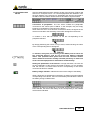
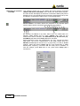
The passive probes are identified by the 8053B or OR03 whether they are
plugged before or after switching on the unit.
The active probes EP333 and EP201 (with internal conversion) are identify by
the 8053B or OR03 only if they are plugged before switching on.
To use the EP201 it’s necessary the Firmware release 3.05 or higher
A more accurate measurement with EP333 and EP201 probes is achieved
setting the filter to 10Hz.
1-24
General information
ELECTRIC FIELD PROBE EP-600
Frequency range
Level range
Overload
Dynamic range
Linearity
Resolution
Sensitivity
100 kHz – 9.25 GHz
0.14 – 140 V/m
> 300 V/m
60 dB
0.4 dB @ 50 MHz/0.3 – 100 V/m
0.01 V/m
0.14 V/m
Flatness
1 – 150 MHz 0.8dB
0.5 – 6000 MHz 1.6 dB
0.3 – 7500 MHz 3.2 dB
(With frequency correction OFF)
0.3 – 7500 MHz 0.4 dB
(Typical with frequency correction ON)
Isotropicity
0.5 dB (0.3 dB typical @ 50 MHz)
Sensors
X/Y/Z reading
Battery reading
Temperature reading
Internal data memory
Six monopoles
Simultaneous sampling of the components
10 mV res.
0.1 °C res.
Serial number
Date calibration
Calibration Factor
SW release.
Battery
Operation time
Panasonic ML621S 3V 5mA/h rechargeable Li-Mn
80 h @ 0.4 S/sec 28 Hz filter
60 h @ 5 S/sec 28 Hz filter
48h for maximum autonomy
17 mm sphere
17 mm sensor
53 mm overall
23g including FO weight (1m)
-10° - +50°
YES
HFBR-0500
¼ - 20 UNC female
Recharge time
Dimensions
Weight
Operating temperature
Software for PC
Optical fiber connector
Tripod adapter
To use the EP600 it’s necessary the Firmware release 3.02 or higher.
General information
1-25
1-26
General information
ELECTRIC FIELD PROBE EP-601
Frequency range
Level range
Overload
Dynamic range
Linearity
Resolution
Sensitivity
10 kHz – 9.25 GHz
0.5 – 500 V/m
> 1000 V/m
60 dB
0.4 dB @ 50 MHz/1 – 500 V/m
0.01 V/m
0.5 V/m
Flatness
0.1 – 150 MHz 0.4dB
0.05 – 6000 MHz 1.6 dB
0.03 – 7500 MHz 3.2 dB
(With frequency correction OFF)
0.05 – 7500 MHz 0.4 dB
(Typical with frequency correction ON)
Isotropicity
0.5 dB (0.3 dB typical @ 50 MHz)
Sensors
X/Y/Z reading
Battery reading
Temperature reading
Internal data memory
Six monopoles
Simultaneous sampling of the components
10 mV res.
0.1 °C res.
Serial number
Date calibration
Calibration Factor
SW release.
Battery
Operation time
Panasonic ML621S 3V 5mA/h rechargeable Li-Mn
80 h @ 0.4 S/sec 28 Hz filter
60 h @ 5 S/sec 28 Hz filter
48h for maximum autonomy
17 mm sphere
17 mm sensor
53 mm overall
23g including FO weight (1m)
-10° - +50°
YES
HFBR-0500
¼ - 20 UNC female
Recharge time
Dimensions
Weight
Operating temperature
Software for PC
Optical fiber connector
Tripod adapter
To use the EP601 it’s necessary the Firmware release 3.02 or higher.
General information
1-27
1-28
General information
ELECTRIC FIELD PROBE EP-602
Frequency range
Level range
Overload
Dynamic range
Linearity
Resolution
Sensitivity
5 kHz – 9.25 GHz
1.5 – 1500 V/m
> 3000 V/m
60 dB
0.4 dB @ 50 MHz/2.5 – 1000 V/m
0.01 V/m
1.5 V/m
Flatness
0.1 – 150 MHz 0.4dB
0.05 – 6000 MHz 1.6 dB
0.03 – 7500 MHz 3.2 dB
(With frequency correction OFF)
0.05 – 7500 MHz 0.4 dB
(Typical with frequency correction ON)
Isotropicity
0.5 dB (0.3 dB typical @ 50 MHz)
Sensors
X/Y/Z reading
Battery reading
Temperature reading
Internal data memory
Six monopoles
Simultaneous sampling of the components
10 mV res.
0.1 °C res.
Serial number
Date calibration
Calibration Factor
SW release.
Battery
Operation time
Panasonic ML621S 3V 5mA/h rechargeable Li-Mn
80 h @ 0.4 S/sec 28 Hz filter
60 h @ 5 S/sec 28 Hz filter
48h for maximum autonomy
17 mm sphere
17 mm sensor
53 mm overall
23g including FO weight (1m)
-10° - +50°
YES
HFBR-0500
¼ - 20 UNC female
Recharge time
Dimensions
Weight
Operating temperature
Software for PC
Optical fiber connector
Tripod adapter
To use the EP602 it’s necessary the Firmware release 3.16 or higher.
General information
1-29
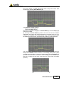
EP-602 Typical frequency response
2.00
[dB]
0.00
-2.00
-4.00
-6.00
-8.00
-10.00
0.001
1-30
0.01
0.1
General information
1
10
100
1000
MHz
10000
ELECTRIC FIELD PROBE EP-333 TRUE RMS
Frequency range
Level range
Overload
Dynamic range
Resolution
Sensitivity
Flatness
0.1 – 3600 MHz
0.15 – 300 V/m
600 V/m
> 66 dB
0.01 V/m
0.15 V/m
0.3 MHz – 3500 MHz 3.0 dB
3.5 MHz – 3200 MHz 1.5 dB
20 MHz – 500 MHz 0.75 dB
0.8 dB (typical 0.5 dB)
> 20 dB
Isotropicity
H-field rejection
Calibration
Temperature error
On board EEPROM
20°C ÷ 60°C ±0.1 dB
0°C ÷ 20°C -0.05 dB/°C
-20°C ÷ 0°C -0.15 dB/°C
385 mm length 133 mm diameter
293 g.
Size
Weight
Typical frequency response for EP333 at 6 V/m nominal electric field
3
[dB]
0
-3
-6
-9
-12
0.1
1
10
100
1000
[MHz]
10000
The EP-333 has been developed for RMS measurement of digital signal with high crest factor for which traditional
diode detectors overestimate.
It is a particular diodes based detector circuital configuration that allows high sensitivity compared to the RMS
termocouple detectors.
Test on COFDM signal (FFT8k, Constellation 64QAM, Crest factor 13dB, guard interval 1/32) have shown that the
overestimation is less than 0.5dB up to 75 V/m on all frequency range of the probe.
The passive probes are identified by the 8053B or OR03 whether they are
plugged before or after switching on the unit.
The active probes EP333 and EP201 (with internal conversion) are identify by
the 8053B or OR03 only if they are plugged before switching on.
To use the EP201 it’s necessary the 8053B Firmware release 3.05 or higher
To use the EP201 it’s necessary the OR03 Firmware release 2.11 or higher
General information
1-31
ELECTRIC FIELD PROBE EP-645
(0.1) 0.3 – 6500 MHz
0.35 – 450 V/m
900 V/m
> 62 dB
0.01 V/m
0.35 V/m
3 MHz – 10 MHz
10 MHz – 1000 MHz
1000 MHz – 3000 MHz
3000 MHz – 5500 MHz
0.8 dB (typical 0.5 dB)
> 20 dB
Frequency range
Level range
Overload
Dynamic range
Resolution
Sensitivity
Flatness
Isotropicity
H-field rejection
Calibration
Temperature error
On board EEPROM
20°C ÷ 60°C ±0.1 dB
0°C ÷ 20°C -0.05 dB/°C
-20°C ÷ 0°C -0.15 dB/°C
317 mm length 58 mm diameter
100 g.
Size
Weight
[dB]
1.5 dB
1.0 dB
1.5 dB
2.5 dB
Typical frequency response for EP-645 probe
3.0
2.0
1.0
0.0
-1.0
-2.0
-3.0
-4.0
-5.0
[MHz]
-6.0
0.1
1-32
1.0
General information
10.0
100.0
1000.0
10000.0
ELECTRIC FIELD PROBE EP-745
0.1 – 7000 MHz
0.35 – 450 V/m
900 V/m
> 62 dB
0.01 V/m
0.35 V/m
3 MHz – 10 MHz
10 MHz – 1000 MHz
1000 MHz – 3000 MHz
3000 MHz – 6000 MHz
0.8 dB (typical 0.5 dB)
> 20 dB
Frequency range
Level range
Overload
Dynamic range
Resolution
Sensitivity
Flatness
Isotropicity
H-field rejection
Calibration
Temperature error
1.5 dB
1.0 dB
1.5 dB
2.5 dB
On board EEPROM
20°C ÷ 60°C ±0.1 dB
0°C ÷ 20°C -0.05 dB/°C
-20°C ÷ 0°C -0.15 dB/°C
317 mm length 58 mm diameter
100 g.
Size
Weight
Typical frequency response for EP745 probe
( dB )
3.0
2.0
1.0
0.0
-1.0
-2.0
-3.0
-4.0
-5.0
-6.0
0.1
1.0
10.0
100.0
1000.0
General information
10000.0
( MHz )
1-33
ELECTRIC AND MAGNETIC FIELD ANALYZER EHP-50C
Electric field
Magnetic field
5 Hz – 100 kHz
0.01 V/m – 100 kV/m
1 nT – 10 mT
200 kV/m @ 50 Hz
20 mT @ 50 Hz
> 140 dB
Frequency range
Level range
Overload
Dynamic
Resolution
0.001 V/m on 8053B Display
1 nT on 8053B display or internal data
0.1 V/m with 8053B Data logger logger
10 nT with 8053B Data logger
Sensitivity
Absolute error
Flatness (40 Hz – 10 kHz)
Isotropicity
Linearity @ 50 Hz
Internal memory
Internal data logger
FFT
SPAN
Start frequency
Stop frequency
E-field rejection
H-field rejection
Calibration
1 nT
± 0.5 dB (@ 50 Hz and 0.1 mT)
± 0.5 dB
± 0.5 dB
(see § 8.4)
± 0.2 dB (1 V/m – 100 kV/m)
± 0.2 dB (200 nT – 10 mT)
1440 data with 1 minute storing; 2880 data with 30 sec storing.
The data can be transferred only to PC
1 measurement every 30 or 60 seconds
Real time FFT analysis
100 Hz, 200 Hz, 500 Hz, 1 kHz, 2 kHz, 10 kHz, 100 kHz
1.2 % of the SPAN
Equal to the SPAN
--> 20 dB
> 20 dB
--2
Internal into E PROM
Temperature deviation (referred to 23°C)
Humidity deviation (referred to 40%)
Size
Weight
Tripod support
Internal battery
Operating time
Recharging time
External DC supply
Fiber optic connection
Firmware update
Autocheck
Operational temperature
Storage temperature
1-34
0.01 V/m
± 0.5 dB (@ 50Hz and 1kV/m)
General information
+/- 0.05 dB between -10 and +23°C, at 40% of relative humidity
+ 0.01 dB/°C between +23 and +50°C, at 40% of relative humidity
+/- 0.05 dB between 20% and 50%, at the temperature of +23°C
+ 0.05 dB/% between 50% and 80%, at the temperature of +23°C
92 x 92 x 109 mm
525 g
Threaded insert ¼”
Rechargeable NiMH batteries (5 x 1.2 V)
>10 hours in normal mode
>150 hours in low-power mode
24 hours with internal data logger (SPAN higher than 200 Hz) in
stand alone mode of operation
< 4 hours
DC, 10 - 15 V, I = about 200 mA
Up to 40 meters (USB-OC)
Up to 80 meters (8053-OC)
Update available through the USB or RS232 port
Automatically when switched on
-10°C to +50°C
-20°C to +70°C
General information
1-35
ELECTRIC AND MAGNETIC FIELD ANALYZER EHP-50E
EHP-50E Main Specifications
When not differently specified the following specifications are referred to operating ambient
temperature 23°C and relative humidity 50%.
Technical specifications of the EHP-50E Electric and Magnetic Field Analyzer
Electric Field
Magnetic Field
Frequency range
Measurement range (1)
Overload
Dynamic range
Resolution (2)
Displayed average noise level (3)
Isotropic result
Single axis
Flatness (@ 100 V/m, 2 µT, 5mV)
(5 Hz ÷ 40 Hz)
(40 Hz ÷ 100kHz)
Anisotropicity (typ)
Linearity (referred to 100 V/m and 1 µT)
5 mV/m ÷ 1 kV/m
500mV/m ÷ 100 kV/m
(146 dB)
200 kV/m
Start frequency
Stop frequency
Rejection to E fields
Rejection to H fields
Calibration
Typical temperature deviation
@ 55 Hz referred to 23°C
30 nV ÷ 10 mV
3 uV ÷ 1 V
(150 dB)
2V
106 dB
110 dB
110 dB
1 nT with 8053B
0.1 nT with EHP-TS SW
1 nT Stand alone
0.1 nV with EHP-TS SW
5 mV/m
3 mV/m
0.3 nT
0.2 nT
30 nV
0.8 dB
0.35 dB
0.8 dB
0.35 dB
0.8 dB
0.35 dB
0.54 dB
0.12 dB
0.2 dB (1 V/m ÷ 1 kV/m)
0.2 dB (200 nT ÷ 10 mT)
-4x10-3 dB/°C within -20 +55 °C
-3
+11x10 dB/% within 10 50 %
+22x10-3 dB/% within 50 90 %
Internal battery
Operating time
Recharging time
External supply
Optical fiber connection
Firmware updating
Self test
Operating temperature
Operating relative humidity (4)
Charging temperature
Storage temperature
-3
-8x10 dB/°C within -20 +23 °C
+13x10-3 dB/°C within +23 +55 °C
-7x10 dB/% within 10 50 %
+10x10-3 dB/% within 50 90 %
92 x 92 x 109 mm
550 g
Threaded insert ¼”
3.7 V / 5.4 Ah Li-Ion, rechargeable
>9 hours in standard mode
24 hours in stand alone mode
< 6 hours
10 ÷ 15 VDC, I = approx. 500 mA
up to 40 m (USB-OC)
up to 80 m (8053-OC)
through the optical link by USB or RS232
automatic at power on
-20 to +55 °C
0 to 95 %
0 to +40°C
-30 to +75°C
Specification are subject to change without notice
General information
-----
---
-3
For each single axis. Ranges to be selected manually
For the lower measurement range
DANL is frequency and SPAN depending. The specified best performance is referred to f ≥ 50 Hz and SPAN ≤ 1 kHz
Without condensation
1-36
--0.2 dB (10 µV ÷ 1 V)
Up to 24 hours regardeless the logging rate.
1 measurement every 30 or 60 seconds
FFT
Simultaneous three axis acquisition
100 Hz, 200 Hz, 500 Hz, 1 kHz, 2 kHz, 10 kHz, 100 kHz, 400 kHz
(500Hz to 100kHz in Stand Alone mode)
1Hz with SPAN 100 Hz; 1.2 % of the SPAN with wider SPAN
Equal to the SPAN
--> 20 dB
> 20 dB
--internal E2PROM
(@ 50% of relative humidity when applicable)
Typycal relative humidity deviation
@ 55 Hz referred to 50% (@ 23 °C)
Dimensions
Weight
Tripod support
0.3 nT ÷ 100 µT
30 nT ÷ 10 mT
(150 dB)
20 mT
1 mV/m with 8053B
0.1 mV/m with EHP-TS SW
1 mV/m Stand alone
Internal memory
Internal data logger
Spectrum analysis method
Acquisition method
SPAN
(1)
(2)
(3)
(4)
AUX input (MMCX Zin 1kΩ)
1 Hz ÷ 400 kHz
---
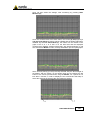
Typical frequency response for EHP-50E Analyzer @ -20dBm (AUX Input)
(dB)
3.0
2.0
1.0
0.0
-1.0
-2.0
-3.0
0.001
0.01
0.1
(kHz)
1
10
100
1000
100
1000
Typical frequency response for EHP-50E Analyzer @ 100V/m (Electric Field)
(dB)
3.0
2.0
1.0
0.0
-1.0
-2.0
-3.0
0.001
0.01
0.1
(kHz)
1
10
Typical frequency response for EHP-50E Analyzer @ 2μH (Magnetic Field)
(dB)
3.0
2.0
1.0
0.0
-1.0
-2.0
-3.0
0.001
0.01
0.1
(kHz)
1
10
100
General information
1000
1-37
ELECTRIC AND MAGNETIC FIELD ANALYZER EHP-200A
EHP-200A Technical specifications
Electric Field
9 kHz ÷ 30 MHz
Magnetic Field Mode A
9 kHz ÷ 3 MHz
@10kHz RBW
0,1 ÷ 1000 V/m
30 mA/m ÷ 300 A/m
3 mA/m ÷ 30 A/m
-80 ÷ 0 dBm
with preamplifier ON
0,02 ÷ 200 V/m
6 mA/m ÷ 60 A/m
0.6 mA/m ÷ 6 A/m
-94 ÷ -14 dBm
Frequency range
Measurement range
Magnetic Field Mode B
300 kHz ÷ 30 MHz
AUX Input
9 kHz ÷ 30 MHz
> 80 dB
> 94 dB
Dynamic range
Measurement range
Resolution
Sensitivity @10kHz RBW (*)
0.01 V/m
0.1 V/m
1 mA/m
30 mA/m
0.1 mA/m
3 mA/m
0.01 dB
-80 dBm
with preamplifier ON
0.02 V/m
6 mA/m
0.6 mA/m
-94 dBm
0,5 dB
0,8 dB
150 kHz – 3 MHz
0,8 dB
300 kHz – 27 MHz
@ -20dBm
@ 166 mA/m
@ 53 mA/m
Flatness
100 kHz – 27 MHz
@ 20 V/m
Anisotropicity @1MHz
Linearity @1MHz
SPAN
RBW
Rejection to E fields
Rejection to H fields
Calibration
Temperature error
Dimensions
Weight
--> 20 dB
0.8 dB
0,5 dB from FS to –60 dBFS
0 to FULL SPAN
1 kHz – 3 kHz – 10 kHz – 30 kHz – 100 kHz – 300 kHz
> 20 dB
--internal E2PROM
0,02 dB/°C
92 x 92 x 109 mm
580 g
selectable ON/OFF, 14dB
2
2
V/m, A/m, uT, mW/cm , W/m
3,7 V – 5,55 Ah Li-Ion, rechargeable
> 12 hours
< 8 hours
10 ÷ 15 VDC, I = approx. 560 mA
up to 40 m (USB-OC)
up to 80 m (8053-OC)
through the optical link
Firmware updating
automatic at power on
Self test
-10 to +50°C
Operating temperature
-20 to +70°C
Storage temperature
(*) The maximum sensitivity is achieved with the filter to 10 kHz
Preamplifier
Units
Internal battery
Operation
Recharging time
External supply
Optical fiber connection
1-38
General information
0,4 dB
---
-----
EHP-200A Technical specifications with 8053B
Electric Field
50 kHz ÷ 550 kHz
500 kHz ÷ 30 MHz
Magnetic Field Mode A
50 kHz ÷ 550 kHz
500 kHz ÷ 3 MHz
Magnetic Field Mode B
300 kHz ÷ 800 kHz
500 kHz ÷ 30 MHz
@10kHz RBW
0,1 ÷ 1000 V/m
30 mA/m ÷ 300 A/m
3 mA/m ÷ 30 A/m
with preamplifier ON
0,02 ÷ 200 V/m
6 mA/m ÷ 60 A/m
0.6 mA/m ÷ 6 A/m
Frequency range
Measurement range
Dynamic range
Measurement range
Resolution
Sensitivity @10kHz RBW (*)
with preamplifier ON
Flatness
Anisotropicity @1MHz
Linearity @1MHz
SPAN
RBW
Rejection to E fields
Rejection to H fields
Calibration
Temperature error
Dimensions
Weight
Preamplifier
Units
Internal battery
Operation
Recharging time
External supply
Optical fiber connection
Firmware updating
Self test
Operating temperature
Storage temperature
> 80 dB
> 94 dB
0.01 V/m
1 mA/m
0.1 mA/m
0.1 V/m
30 mA/m
3 mA/m
0.02 V/m
6 mA/m
0.6 mA/m
0,5 dB
0,8 dB
150 kHz – 3 MHz
0,8 dB
300 kHz – 27 MHz
@ 166 mA/m
@ 53 mA/m
100 kHz – 27 MHz
@ 20 V/m
--> 20 dB
0.8 dB
0,5 dB from FS to –60 dBFS
50 kHz to FULL SPAN
1 kHz – 3 kHz – 10 kHz – 30 kHz – 100 kHz – 300 kHz
> 20 dB
--internal E2PROM
0,02 dB/°C
92 x 92 x 109 mm
580 g
selectable ON/OFF, 14dB
V/m, A/m
3,7 V – 5,55 Ah Li-Ion, rechargeable
> 12 hours
< 8 hours
10 ÷ 15 VDC, I = approx. 560 mA
Up to 80 m
through the optical link
automatic at power on
-10 to +50°C
-20 to +70°C
(*) The maximum sensitivity is achieved with the filter to 10 kHz
General information
1-39
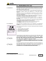
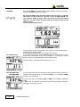
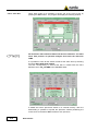
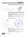
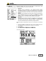
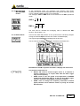
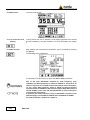
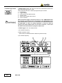
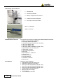
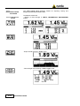
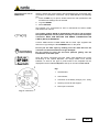
1.7 Front panel
of PMM 8053B
Key:
1. Probe connector;
2. Display;
3. Fiber
optic
Input/Output
for
additional probes or
USB
or
RS232
interface via fiber optic
link;
4. RS232 interface;
5. Battery charger input,
from 10 to 15V DC,
500mA;
6. Securing screws to
tripod;
7. Alphanumeric
keyboard;
Fig. 1-1 Front panel
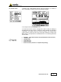
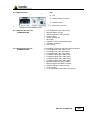
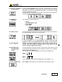
1.8 Side panel
of PMM 8053B
Key:
1. Connection
to
OR02/OR-03
Optical
repeaters, GPS, EHP50C or EHP200A fiber
optic link;
2. Wired RS232 interface
for direct connection to
the PC;
Fig. 1-2 Side panel
3. Battery charger
connector (12V, 0.5A)
1-40
General information
2 - Installation and use
2.1 Introduction
This section provides the information required for installing and using the
PMM 8053B General Purpose Field Meter. For information regarding the
use of the accessories, see Chapters 8, 9 and 10 of this Manual.
Information is included regarding initial inspection, power requirements,
interconnections, work environment, assembly, cleaning, storage and
shipment.
2.2 Preliminary
inspection
Inspect the packaging for any damage.
If the packaging or anti-shock material have been damaged, check
that the contents are complete and that the meter has not suffered
electric or mechanical damage.
Check that all the Accessories are there against the checklist found
with the apparatus.
Inform the carrier and NARDA of any damage that has occurred.
2.3 Work environment
The work environment of the Accessories, must come within the following
conditions:
From -10°C to +40°C
• Temperature
< 90% relative
• Humidity
The meter must be stored in a clean and dry environment, free from acid
dusts and humidity.
The storage environment must come within the range of the following
conditions:
From -20°C to + 70°C
• Temperature
< 95% relative
• Humidity
2.4 To return for repair
When the meter needs to be returned to NARDA for repair, please
complete the questionnaire appended to this User’s Manual, filling in all the
data that will be useful for the service you have requested.
For reducing the period of time required for the repairs, it is necessary to be
as specific as possible in describing the problem. If the problem only occurs
in certain circumstances, please describe in detail how it happens.
If possible it is better to reuse the original packaging; making sure that the
apparatus is wrapped in thick paper or plastic.
Otherwise, use strong packaging by using a sufficient quantity of shock
absorbent material around all sides of the meter to ensure that it is compact
and does not move around inside the package.
In particular, take every precaution to protect the front panels.
Finish the package by sealing it up tightly.
Apply a FRAGILE label to the package to encourage greater care in its
handling.
2.5 To clean the meter
Use a dry, clean and non-abrasive cloth for cleaning the meter.
Do not use solvents, acids, turpentine, acetone or other similar
products for cleaning the meter in order to avoid damaging it.
Document 8053BEN-40918-3.16 - © NARDA 2014
Installation and use
2-1
2.6 PMM 8053B
To install and use
The PMM 8053B General Purpose Field Meter can work only with PMM
isotropic probes within wide range and frequency fields and its accessories.
Installation of PMM 8053B is very easy. Simply insert the probe into the
special connector at the top of the apparatus and switch it on.
The probe may be connected to the apparatus whether it is switched
on or off without damage. To avoid damage to the probe connector,
the spigot (red dot), found in the external part of the probe connector,
must be put facing the front part of the meter.
To connect or disconnect the probe, hold onto the metallic connector.
When inserting or removing the probe, holding on to the support or
the head may cause damage to the probe.
When measuring fields emitted from transmitting antennas, it is
important to place the probe with the handle of the support
perpendicular to the polarisation of the antenna to avoid interference
with the measurement (normally the probe should be positioned in
horizontal). This is especially so when analysing signals in the range
of few megahertz.
2.7 RF signals of
dangerous fields
The probe of PMM 8053B uses highly sensitive components.
Do not insert the probe in an electric or magnetic field that is higher
than the maximum permitted for the probe in use, even if you do not
perform any measurement.
Whether the PMM 8053B is switched on or off or even if the probe is
not connected to the meter, damage may be caused to the internal
diodes when strong fields radiate the probe.
2.8 Battery charger
The battery charger supplied with the meter can work at either 50 Hz or 60
Hz with a supply voltage range between 100 and 240 Volt.
It is supplied with different connectors to the supply mains in accordance
with the various national standards.
2.8.1 To substitute the
mains connector
To substitute the mains connector, simply remove the one installed on the
battery charger and replace it with the one that is in compliance with its use.
2-2
Installation and use
2.8.2 To check the
internal batteries
If the internal batteries are to have the greatest autonomy, we recommend
that a full recharging cycle be carried out before using the meter.
To do this, go through the following procedure:
• Connect the battery charger to the power socket
• Link the output connector of the battery charger to the input CHARGER
on the side panel of the meter
• PMM 8053B will switch on automatically, after making a sound
produced by the internal buzzer, the display will be activated and the
meter will start its auto-check and begin the procedure for recognising
the probes.
• The main window will therefore be activated and the status of the
charge (CHG) of the battery will be displayed in the STATUS box
Indications of the battery in the STATUS box:
The status of the charge of the battery is displayed in the top left-hand
corner of the STATUS box. The symbol of a small battery will be filled up
proportion to the status of the battery charge.
The battery charger will be automatically stopped when one of the following
occurs and a small connector will be displayed relating to a letter indicating
the end of the recharging cycle.
Display of the following letters means:
V – The voltage of the batteries has reached 1.45 V/element (7.25 total),
and therefore the recharging cycle is complete.
H – The recharging cycles has lasted for more than 4 hours.
T – The temperature of the batteries, compared to the temperature stored
after ten minutes recharging, has increased more than 10 °C, or the
temperature of the battery has reached 65 °C.
When the recharging cycle is finished, the PMM 8053B is ready for use.
To avoid damage to the batteries, when the T symbol appears, the
recharging cycle is stopped automatically.
To finish the recharging cycle wait for about ten minutes for the
batteries to cool down then reconnect the battery charger.
Battery charger: DC, 10 - 15 V, ~ 500 mA
-
+
Connector:
ALWAYS connect the battery charger to the mains power BEFORE
connecting the DC output to PMM 8053B. The battery charger has an
internal protective circuit that will not let it work if there is a load
connected to the battery charger before the connection to the mains
is activated.
In order to safeguard the features of the batteries, it is crucial to have
a complete recharge before storing them for periods longer than 4
months. Therefore, it is warmly suggested recharging the batteries at
least every 4 months even though the device has not been used.
Installation and use
2-3
During measurement, it is necessary to disconnect the battery
charger as it introduces noise into the measurements equal to about
0.3% of the full scale of the probe in use, when there is no field.
For example, using a EP-330 probe, which has a full scale of 300 V/m,
the noise N introduced by the battery charger is equal to:
N=
300 V / m × 0,3
= 0,9 V / m
100
This phenomenon rapidly reduces with the increase of intensity of the
field applied to the probe. An actual field of 1.5 V/m may be indicated
as equal to 1.8 V/m while an actual field of 6 V/m may be indicated as
equal to 6.1 V/m. In all cases the recharging cable must be kept far
away from the probe as well as from the sources of the field itself.
Recharging does not produce any error when the probe is installed at
least a few meters away from PMM 8053B meter via PMM OR02/03
Optical Repeaters.
2-4
Installation and use
3 – Instructions for use
3.1 Introduction
The PMM 8053B General Purpose Field Meter is designed to be simple
and rapid in use and, therefore, able to be used even by personnel with
little expertise with this type of meter.
The commands are entered through a 16-key alphanumeric keyboard and
the relative software functions are displayed on a wide liquid crystal
display.
The upper four keys of the alphanumeric keyboard are used for directly
selecting the desired function indicated on the corresponding bar of the
menu of the LCD display.
Some panels enable the user to simply select the function by shifting up
and down the commands with the arrows on the menu bar.
A command is generally automatically repeated, either in a constant or
increasing manner according to the selected command, by holding the
keys down.
The remaining 12 keys of the alphanumeric keyboard are used for entering
various kinds of data according to the chosen set-up.
The BACK key enables the user to return to the previous operation.
The POWER key allows the meter to be switched on or off.
3.2 To switch-on
Once the probe is inserted the meter can be switched on by pressing the
POWER key. A long beep will confirm that the meter has been switched on.
The set-up routine will then be run and the following information will appear
on the display:
1.
2.
3.
4.
Version and date of the firmware;
Control state of the keyboard;
Autocalibration of the input stage;
Control of the integrity of probe.
If the probe has not been previously connected to the meter Step 4 will
not be performed and the word “NONE” will appear in the ”Probe”
box in the main window. If, instead, the probe is not working properly
the word “FAIL” will appear in relation to the non-functioning axis
(e.g., Z:OK, Y:FAIL, X:OK) and a beep will be emitted.
To use 8053B with EHP-50C is mandatory to have the 8053 firmware
2.30 or higher. To use it with EHP-50E the 8053 firmware 3.16 or higher
is required.
The time required for the internal calibration of the meter depends on
the noise filter chosen. If the filter is set at 10 or at 20 Hz, the
calibration process will take longer than with higher frequencies.
For normal use, we recommend setting the filter at 40 Hz.
Document 8053BEN-40918-3.16 - © NARDA 2014
Instructions for use
3-1
3.3 Main menu
Once the set-up routine has been completed, the meter will display the
window of the main menu:
1
2
3
4
5
This window is divided into lines which mean the following:
1. The top line is subdivided into two boxes:
1a) The box on the left displays the type of probe that is connected and
the date of calibration or any accessory and the status of the charge
of its batteries;
1b) The box on the right displays the general status of the various
parameters and setting that will be explained in greater detail later;
2. The second line from the top displays the digital value of the reading,
according to the current UNIT;
3. The third line from the top displays the analog value of the reading, and
its display can be in either linear or logarithmic format;
4. The fourth line displays various data in accordance with the set MODE;
5. The last line on the bottom displays the functions assigned to the four
top keys.
Other Informations found in the various boxes are described in more detail
in the next paragraphs.
3-2
Instructions for use
3.3.1 Data about the
probe
The box at the top on the left, labelled
Probe, displays the type of probe
connected to the meter and, for probes
2
with internal E PROM, the date of
calibration also appears.
When no probes are connected, the
word NONE appears.
The example of the EP330 probe linked
to the 8053B via the OR03 Optical
Repeater, displays the status of the
batteries of the OR03.
Only NARDA can update correctly the calibration factors in the
2
E PROM.
NARDA calibration services are recommended to achieve the best
performances from the system
3.3.2 Status box
The box at the top on the right, labelled the Status box, displays the
general status referring to the various parameters and setting of the meter
as set out in the following:
1. Status of the battery charge;
2. Voltage of the battery;
3. Acquisition time of the Data logger or storage mode;
4. Plotting time (Plot) or the number of data samples acquired (Sample);
5. Alarm indicator (Alarm) and the setting of the alarm level;
6. Frequency used to provide automatic flatness correction.
Instructions for use
3-3
3.3.3 Digital reading
Depending on the selected measurement unit, the meter will display the
field measured by the probe.
This indication is calculated according to the following formula which uses
every single axis value:
V/m tot =
E x ²+E y ²+E z ²
When the field intensity is lower then the specific sensitivity of the probe in
use, the word LOW will appear on the display like in the following window:
If 8053B is turned on keeping the Key 5 depressed (an keyboard error
will appear during the turn on procedure, it should be ignored), it is
possible to read all fields starting from about 0 V/m. Of course these
very low values are affected by a high errors and should not be used
for any evaluation purpose.
3.3.4 Analog bar
3-4
The intensity of the measured field is also displayed in analog form. The
analogical reading may be set either in logarithmic or linear format.
From menu SET move the pointer on Bar and selected Linear o
Logarithmic
Also a TAG is provided to indicate that the alarm is ON and it is located
proportionally.
Instructions for use
3.3.5 Main Function keys
The function keys enable the user to select all the operational modes.
When the PMM 8053B is switched on the following menu appears:
The relative functions are:
select a different measurement units
select a different operational or storage mode The MODE key
runs the SAVE-MODE function of the data logger
change the contrast and intensity of the display
enter the main settings of the meter and select other secondary
functions
3.4 UNIT
By activating the UNIT key, the user can select the measurement unit he
desires, depending on the installed probe.
When an electric field probe is installed, the following units of measurement
can be selected:
• V/m, A/m, mW/cm , W/m
2
2
When using EHP-50, the units are: V/m, kV/m, µT and mT.
When using HP-050/051 the unit is in µT.
Any time the user decides to use a non-primary but derived
measurement unit, the following warning will be displayed: WARNING
Correlated UNIT to notify the user that the result displayed is derived
from an internal calculation and not directly from a measurement, the
conversion is valid in far-field conditions.
The applied formulas are:
H(A/m) = E(V/m)/377(Ohm)
S(W/m²)=E(V/m) x H(A/m)
Using the BACK key enables the user to return to the main menu.
Instructions for use
3-5
3.5 MODE
By pressing MODE, the PMM 8053B allows different modes for acquiring,
storing and displaying data to be used.
By pressing MODE with the DATA Logger ON, the display of 8053B
will switch off after about 90 seconds. In this modality 8053B can
store data for about 40 hours. When you press any key the display
switch on and then switch off again after 90 seconds to preserve the
battery charge.
The window displayed will be:
3.5.1 ABS/% mode
The low power mode is used together with Logger xxxs Def and also when
using EHP-50C and EHP-50E.
In this mode the display will turn off during the acquisition.
In this operational mode, PMM 8053B displays the absolute value of the
three vector components of the measured field or by pressing a second
time the same key, 8053B displays the percentage value.
The total value is calculated as described in par. 3.3.3.
3.5.2 MIN-MAX/AVG
MIN-MAX/RMS
In this operational mode, the maximum and minimum values as well as the
average value expressed as an arithmetic (AVG) or as a quadratic (RMS)
average can be displayed.
To select the type of averaging (AVG or RMS), use the SET operational
mode.
In SET mode, it is possible to select among several averaging period. See
paragraph. 3.7.2 and 3.7.6.7-8.
3-6
Instructions for use
3.5.3 PLOT mode
In PLOT mode, PMM 8053B acquires data and displays it in relation to
time. The display is similar to that in the following example:
This example uses the COUPLED mode
This field versus time function is designed in order to verify the stability of
the field while the time goes by, showing a graphic display very simple to
understand. This graph cannot be saved or printed. The selected time
scale is shown in the box at the top on the right. Selection is made in the
SET mode in correspondence to the PLOT T line. The following selections
can be made:
•
•
•
•
•
•
Coupled
(the fastest mode; the speed depends from the Filter)
1 min/division
2 min/division
10 min/division
30 min/ division
60 min/ division (4 hours to complete the plotting)
Instructions for use
3-7
3.5.4 DATA logger
In the DATA logger mode, the user can store the data of the
measurements taken and saved in a file. The DATA logger function will
collect data from any probes connected directly to 8053B or by using the
optical repeaters OR-02 or OR-03, or using the EHP-50C and EHP-50E. It
does not collect any data when using GPS module. In SET menu, the user
can define the sample rate, the different acquisition modes, and how long
the measurement will take. All the generated files are numbered
progressively and contain:
• the date and time when the measurement began
• the average value
• the value of each single data stored
• the user’s comment
As soon as the DATA logger key is pressed, the first file appears on the
display with the available commands on the line below.
This is an example of the display:
1. The first line indicates the number of the file (in this case 1) and the
entire time taken to carry out the measurement (in this case 11
seconds);
2. The second line displays the date of the measurement;
3. The third line shows the time when the measurement began;
4. The fourth line displays the average value calculated (AVG or RMS);
By shifting with the arrows, the individual readings taken are displayed,
point-by-point according to the logger time selected in the SET menu.
In the Time line, the time relating to each measurement will be
displayed.
5. The fifth line indicates the comment entered by the user.
To enter a comment, press an alphanumeric key and then press
The function keys have the following commands:
.
begins data acquisition
selects previous data
selects subsequent data
selects a different file
By holding the arrow keys down, the user can shift between stored
data and data shown on the display.
The same occurs by pressing
3-8
Instructions for use
to select stored files.
3.5.4.1 To begin storing
data
To begin a new measurement and new data acquisition, press the shift key
(at the bottom on the right side) for selecting an next empty record as seen
in the following example:
Then press the RUN key to start the measurement. Before beginning the
measurement, 8053B will display the number of records still available for
storage and will wait for the user to confirm by pressing the OK key.
Now, press OK to start the acquisition.
Instructions for use
3-9
After 90 seconds that the logger has been run, if 8053B is in the menu
MODE (the default menu at the beginning of logger), the display
switch-off (SAVE-MODE function). The supply current is reduced
about 40-45%. Display will switch on in the following way:
•
•
At the pressure of any key (excluding POWER key). In this case
the key’s function isn’t execute (to avoid doing a wrong function)
At the end of acquisition time.
The display isn’t switch off if the menu is different by MODE
In this situation is possible to leave the device ON over the 90 seconds
presets after the last key pressure.
Pay attention to do not press the power key when you switch on the
display to the SAVE-MODE function.
If the user overwrites a record that has already been stored, all
subsequent records will be deleted. For example, the user has already
stored records 1 to 4 with four different measurements. Having then
begun another measurement going to record # 2, records # 2, 3 and
4 will be deleted and the new measurement will be stored in record #
2.
The user can quit data acquisition manually by pressing the STOP key
or automatically after a certain period of time defined in the SET menu
by selecting Log. End.
Data acquisition can, nevertheless, be stopped at any moment,
independently of the set time of acquisition, by pressing the STOP
key.
3-10
Instructions for use
3.5.4.2 To enter a
comment
Any time data are stored, up to 40 characters of text can be linked to the
measurement for identifying the place where the measurement was taken
or other useful information.
To enter a comment, use the alphanumeric keyboard.
The following is an example:
Edit keys have the following meanings:
shift the cursor to the right
shift the cursor to the left
go back a space deleting the character on the left
enter the added text
PMM 8053B has an alphanumeric keyboard of which 11 keys are used for
entering (numeric or alphabetic) data, for making comments or for
recording the locality where the measurements were taken.
For each key, there is a choice among 4 characters. The first time the key
is pressed, the first character will be selected, pressing the key twice in
quick succession, the second character will be selected and so on,
pressing it four times will select the following corresponding number, after
which come the same letters in lower case.
The 0 (SP)-* has four functions: 0, blank space, - e *.
It is necessary to press the key very quickly to select the following
character or number, otherwise the editor will move on to the next.
Instructions for use
3-11
3.6 To control the LCD
display
This key gives the user the possibility of adjusting the contrast and lighting
of the LCD display to adapt it to the light in the environment or to be able to
see it better.
The display will show the following:
This function regulates contrast. Press + o – to increase or decrease it.
This function regulates the back lighting. Press + o – to lighten or darken it.
By pressing the BACK key the user can return to the Main Menu at any
time.
3-12
Instructions for use
3.7 SET function
Pressing the SET key permits the user to enter a window where he can
select the main parameters and settings for the measurements.
The following menu is displayed:
The available function keys for selecting any functions are the following:
To go up in selecting. The selected function has a black
background.
To go down in selecting. The selected function has a black
background.
To select the desired setting by rotating among those that
are available. Each time this key is depressed a new function
will appear in sequence.
This key is used to change from RMS to AVG averaging
mode. It appears only when average is selected.
To turn ON or OFF the Alarm or Frequency.
This key appears only when Alarm or Freq are selected.
To enable/disable the beep when the keys are pressed and
during logger sessions (with the exception of the initial beep
when the meter is switched on).
Instructions for use
3-13
3.7.1 Alarm function
This function can be used in defining the alarm level or to be used with
Over Limit feature.
When the field being measured exceeds the set alarm threshold, the
following functions are enabled:
1. The buzzer is activated and a small blinking symbol appears near the
symbol of the loudspeaker.
2. The set alarm threshold will be displayed on the analog bar with a
darker band that shows whether the measurement is above or below the
set limit.
3. PMM 8053B is enabled to acquire date if the Logger mode function is
set on Over Limit.
4. Depending on the Serial setting (see Serial function paragraph) alarm
signal will be available to the optical or wired connector.
To set the threshold value, it is necessary to type it in with the alphanumeric
keyboard and then press the Enter key. At this point the alarm can be
enabled or disabled on the set threshold by pressing the ON-OFF key.
This function allows the user to be acoustically warned when the field
exceeds a certain threshold without the need to look at the display; it
is interesting for example during the pre-analysis of any device under
test.
It is also a good way to perform long acquisitions without wasting
memory space by saving useless data. The field will be logged into
the memory only if it exceeds the setted threshold, and both the level
and the time of the measurement are saved.
If you are using any EHP-50 with an alarm above 300 V/m and then
another probe is connected with lower full scale (e.g. EP-330), the
alarm will be always beeping.
It is necessary to enter SET and define a new alarm according with
the new range of the used probe or turn OFF the alarm function.
3-14
Instructions for use
3.7.2 Linear average AVG All the average measurements taken by PMM 8053B will be made
depending on the AVG or RMS selection.
or quadratic
To select AVG or RMS use the key at the bottom on the right in the SET
average RMS
function.
Both averages will be calculated on the basis of the following settings:
•
•
•
•
•
•
•
•
•
Last 32 samples
30 sec
1 min
2 min
3 min
6 min
10 min
15 min
30 min
The Average value is displayed in the main window together with the
Maximum and Minimum values. After PMM 8053B has acquired a sufficient
number of data or the time set in this menu has elapsed, the average
measurement will appear in the main display with a small ν symbol as
shown in the following example.
After the
ν symbol is appeared the shown average is the rolling averaging.
PMM 8053B will re-start to calculate a new averaging, which will
overwrite the previous one, every time the MIN-MAX/AVG (or MINMAX/RMS) key is pressed; the accumulated averaged value will be
displayed after the ν symbol.
This value can not be saved into the internal memory of 8053B.
The number of samples used to perform the average calculation will
depend from the Filter selected. For example, if the Filter is set to
10Hz the 8053B will collect less data than when using faster filter like
80 Hz.
By using the Data logger, the sample rate is always timed by the
selected acquisition time. At the end of an acquisition, the number of
data collected, used to calculate the averaging value will be different
from the number of samples used to perform MIN-MAX/AVG.
The result will be a different Average value calculated by the Data
Logger compared with the average value displayed on 8053B.
Only if the field will remain stable (same value for all the time required
by the Data logger), the results will be the same.
Instructions for use
3-15
3.7.3 Freq function
By entering the known frequency value, PMM 8053B will correct the
measurement taken by using the corresponding correction factor included
in an internal table of the probe. This enables an extremely precise
measurement of the field level at the selected frequency to be given.
The selected frequency will be displayed in the Status box of the main
window.
The frequency will always be entered in MHz except for HP-050/051 probe,
which is in Hz.
This function will not appear when using EHP-50 analyzers.
This function can only be used when 8053B is measuring a field
generated by a single frequency (e.g. inside an anechoic chamber) or
you are very close to the broadcast transmitter.
3.7.4 Plot function
This function shows the intensity of a field over a period of time. The
possible time scales are:
• coupled (where the speed of the reading depends on the selected filter)
• 1 min/div
• 2 min/div
• 10 min/div
• 30 min/div
• 60 min/div.
This display can not be printed or saved. It offers only graphic overview of
the field variation versus time.
3.7.5 Serial function
This function is used to transfer data to a PC or to acquire data from an
optical repeater, probes with built-in optical repeater or GPS module. As an
alternative it is possible to send the Alarm status to the Wired or Optical
connector.
The choices are:
• Wired  via a wire.
• Optical  via fiber optic link.
• Alarm Wire  Alarm output to TX terminal of Jack connector:
• Alarm OFF: TX terminal voltage as IDLE (or SPACE) status of RS232 standard (~ -9V)
• Alarm ON: TX terminal voltage as MARK status of RS-232 standard
(~ +9V)
The TX signal corresponds to pin 2 of the DB9f connector and pin TIP
of the jack 2.5mm.
• Alarm OPT  Alarm output to TX terminal of optical connector. The
operation is similar to the preceding one but the alarm signal is fed
through the optical fiber. In normal condition the output LED is off, it will
turn ON as soon as the alarm threshold is exceded.
When using optical link to the PC, it is necessary to use the USB-OC or
8053-OC.
When using Optical link the Wired port is disconnected. Therefore
you can not get data to the PC while you are using any EHP-50 or OR02/OR-03 or GPS module.
3-16
Instructions for use
3.7.6 Logger function
With this Logger function, PMM 8053B can be used as data acquisition
system. It can acquire data and save field measurements for long periods,
storing the date and time of each measurement. Furthermore, given that
the internal memory is dynamically indexed, many groups of measurements
– even those acquired in different ways with different probes – can be
stored. Each group can be identified with a user’s comment of 40
characters together with the date and the time that the measurement
began.
To meet the widest possible needs, PMM 8053B has various modes for
storing data:
1. Over Limit data are sampled every second and stored for the whole
time during which the value is higher than the limit set with the Alarm
function.
2. Manual data are stored every time the GET key is pressed.
3. Data change data is stored either when the value is 25% higher or
lower than the previous one or after an hour has elapsed since the last
variation.
4. 1s Fix the highest field value logged during the span of one second is
stored.
5. xxxs Def the highest value logged during the span of xxx seconds
defined by the user, the value (between 10 and 900 seconds) can be set
with the alphanumeric keyboard.
6. xxxs Def LP this is the Low Power mode, only to be used with the
EHP50A/B/C/E probes which works like the xxxs Def mode, except that
the probe is placed on Stand By between one measurement and
another reducing energy consumption to a minimum and therefore
increasing the autonomy of the batteries of EHP50A/B/C/E.
7. AVG/RMS (6 min-6) the AVG or RMS average value logged during a 6minute span is stored (the stored value will be AVG or RMS depending
on the selected mode).
8. AVG/RMS (6 min-1) the AVG or RMS average value logged during a 6minute span is stored. After this period of time, the operation is repeated
minute by minute, excluding the values red in the first minute and adding
those read in the next up until the last (the stored value will be AVG or
RMS depending on the selected mode).
Instructions for use
3-17
3.7.6.1 Over Limit
This function is quite useful to get only the data exceeding the threshold
defined by the user with the Alarm function.
8053B performs about one measurement every second and stores the field
values for the whole time during which the value is higher than the limit.
When an acquisition, by using Data Logger, has been performed PMM
8053B will show the following display:
In the Status window are shown: the function O.Lim enabled and the
number of the acquired points (in this example 18 points).
The Average function is not enabled because the measured data have no
time relationship each other.
Depressing the arrows UP and Down, it is possible to see each individual
measurements.
In this example the record # 8 shows 7.68 V/m.
3-18
Instructions for use
3.7.6.2 Manual mode
This mode of operation is useful to perform mapping over a specific
territory.
For example, under power lines towers is possible to built a map of the
fields versus the distance from the center of the tower by using 8053-RT
connected to a metric wheel. Each time the wheel performs one turn, it will
activate a signal connected to 8053-RT and the remote trigger will activate
the GET command.
In Manual mode, the time (date and hour) of measurement for each field
value will also be stored.
To use the Manual option, take the following steps:
• In SET mode, select Logger and then Manual.
• Exit SET mode with the BACK key.
• Select MODE and then Data Logger (the Data Logger
automatically goes to the last saved record), to select a new
•
•
measurement record press the
key.
Then press RUN and confirm the beginning of manual measuring
by pressing OK.
At this point, measurements can be acquired manually by
pressing the GET key or via the 8053-RT Trigger accessory. To
quit storage in the current record press BACK and then STOP.
Instructions for use
3-19
3.7.6.3 Data change
This function is used to control the stability of the broadcaster transmitters.
In this mode of operation the 8053B stores fields and the time when the
value is 25% higher or lower the previous one.
Also in this mode of operation the Average function is disabled.
3.7.6.4 1s Fix
This mode allows 8053B to store the data at 1 second interval. The sample
rate is defined by the Filter, for example with 40 Hz filter 8053B performs 3
measurements/sec. The highest value of these measurements will be
saved into the internal memory of 8053B.
The display shows, also, the number of points stored
(e.g. 43 Pts = 43 points).
This mode should not be used with EHP-50A/B/C/E because it is too
fast compare with the time to perform the FFT analysis of ELF probe.
3-20
Instructions for use
3.7.6.5 xxxs Def
In this mode the user can apply for any storing interval from 10 to 900 sec.
To replace the old number with a new one, simply type over the new storing
interval and press the key
.
If it is necessary to modify the number before making it valid with enter key
or cancel the operation, to use ESC or BACK SPACE keys.
After depressing
the 8053B will return to the main display showing
the new time interval (in this example 600 sec).
Now 8053B is ready to perform a new data acquisition. Also in this
mode of operation, 8053B will perform a number of measurements
according to Filter speed and will store the highest value of all data
measured over 600 seconds interval (in this example).
Instructions for use
3-21
3.7.6.6 xxxs Def LP
This mode works like the xxxs Def mode, except that the probe is placed in
Stand-By between one measurement and another reducing energy
consumption to a minimum and therefore increasing the autonomy of the
batteries of EHP50A/B/C/E. See chapter 8 for more details.
In the main menu, 8053B will show the symbol L near to the storing interval
number.
In this example, only one measurement is taken every 600 seconds.
By using this option with other probes, the apparatus acts in the same way
as for the xxxs Def option.
3.7.6.7 Avg(RMS) 6min-6 In this mode of operation, 8053B acquires data for 6 minutes and then
calculates the average value (Linear or quadratic according to AVG or RMS
selection) and stores the result inside its internal memory. This operation
will be repeated every 6 min until the Log. End reaches its value or the Data
logger is manually terminated.
The symbol Σ6-6 is shown on main display.
The Data logger memory will be filled up with field’s values equidistant of 6
min. Each value is the result of the averaging over 6 min.
3-22
Instructions for use
3.7.6.8 AVG(RMS) 6min-1
This mode of operation performs the rolling 6 minutes averaging with 1 min.
resolution. 8053B will store in the first record the value averaged over 1
min; the second record will have the average value over 2 min; the third
record will have the average value over 3 min and so on.
After 6 min, 8053B will store the 6 minutes average. Then 8053B will start a
new computation excluding the values red in the first minute and adding
those read in the next up until the last (the stored value will be AVG or RMS
depending on the selected mode).
The symbol Σ6-1 is shown on main display.
The internal memory of the Data Logger will be filled up with values
equidistant of 1 min. Each of them is the average value over the last 6
minutes.
Instructions for use
3-23
3.7.6.9 Memory property
Mode
Sampling 1 s
Sampling xxx s
(10 - 900 s)
AVG 6 min.
RMS 6 min.
Data change
Over the LIMIT
Manual
The 8053B has a 16kB standard memory, and a 52kB. The following table
is refer to standard memory:
Sampler
Data saved
Occupied space
Bytes
Max Data
Points
Max storage time
Unconditional
every second
Only values
(Peak within 1 s)
Header (88)+2*N
>26000
>7h 13’
Only values
Header (88)+2*N
(Peak within xxx s)
>26000
72h 13’ – 6500h
Unconditional
every xxx
seconds
Unconditional
every 360
seconds
Unconditional
every 360
seconds
25% of the
variation or
every hour
every second
while the field is
above the limit
Manual
Only values
(AVG of 6 min))
Header (88)+2*N
>26000
>2600h
Only values
(RMS of 6 min))
Header (88)+2*N
>26000
>2600h
Values and time of Header (88)+4*N
each one
>13000
Values and time of Header (88)+4*N
each one
>13000
Up to 539 day
lim. From Max
Data Point
>3 hours over the
limit
Values and time of Header (88)+4*N
each one
>13000
-----------
The number of records able to be stored in PMM 8053B can easily be
calculated as follows:
53248/(88(header) + occupied space)
For example, up to 578 records (each with its comment, date and
time) with data acquired manually (16300/92) can be stored.
When data storage begins in an already occupied group, all the data
stored previously will be overwritten and therefore lost. This means
that if the user needs to keep groups of data that have already been
stored, he will need to carry out a new acquisition in a new record
following the last one that was used.
3-24
Instructions for use
3.7.7 Log. End function
This function determines how much time will be required for data
acquisition. The possible choices are:
•
•
•
•
•
•
•
•
•
Manual
1 min
2 min
4 min
6 min
12 min
20 min
30 min
60 min
acquisition will be stopped manually
acquisition will stop after 1 minute
acquisition will stop after 2 minutes
acquisition will stop after 4 minutes
acquisition will stop after 6 minutes
acquisition will stop after 12 minutes
acquisition will stop after 20 minutes
acquisition will stop after 30 minutes
acquisition will stop after 60 minutes
It is, nevertheless, possible to quit data acquisition in all operational
modes by pressing STOP.
To store data for a time longer then one hour it is necessary to
choose the Manual end mode or connect the 8053B to a PC running
8053-SW02 data acquisition software.
3.7.8 Bar function
This is used to select the linear or logarithmic scale for the analog bar.
3.7.9 Filter function
PMM 8053B has a low-pass filter to reduce noise during measuring. One of
the following can be selected:
•
•
•
•
10 Hz
20 Hz
40 Hz
80 Hz
is the default filter
Acquisition time can vary depending on the selected filter:
• 900 ms with 10 Hz filter
• 450 ms with 20 Hz filter
• 250 ms with 40 Hz filter
• 150 ms with 80 Hz filter
This filter is not used with EHP-50A/B/C/E.
A more accurate measurement with EP333 and EP201 probes is
achieved setting the filter to 10Hz.
The selection of the filter will modify the following functions:
- PLOT Coupled mode: the scroll rate will become slow with
10Hz filter but faster with 80Hz;
- AVG or RMS mode: the number of samples used for the
calculation will change;
- Logger mode: the number of samples from which to pick the
worst value (the highest) will change.
Instructions for use
3-25
3.7.10 AutoOFF function
PMM 8053B can be switched off either manually or automatically after it
has been on for a defined period without the need to press any keys:
• Disabled
• 10 min
• 60 min
manual switch-off
PMM 8053B will be switched off after 10 minutes
PMM 8053B will be switched off after 1 hour
This function is important for reducing battery consumption.
If the Logger function is active, that is, if the meter is storing data, the
AutoOFF function is automatically deactivated until the end of the
programmed acquisition.
3.7.11 Time function
This function allows the user to set the internal clock.
Use the alphanumeric keyboard to enter the time in the following format:
hh.min.sec.
Then press Enter
3.7.12 Date function
to activate the set value.
This function allows the user to set the date in the internal calendar.
Use the alphanumeric keyboard to enter the date in the following format:
day.month.year.
Then press Enter
to activate the set value.
Control of the date in PMM 8053B is in full conformity with the Year 2000.
3-26
Instructions for use
4 - Applications
4.1 What is
electrosmog?
4.2 Observations about
the risks
4.3 Measurement of
power distribution
lines
Electrosmog is a popular term used to describe any phenomenon or
problem associated with artificially generated electric or magnetic pollution.
Any electric or electronic device may cause an environmental risk.
All motors, electronic workstations, AM or FM broadcasting transmitters,
TVs, electric ovens, manufacturing machinery, cellular telephones and
stations can generate potentially hazardous electric or magnetic fields.
Anybody, both at work and elsewhere, can be exposed to sufficiently strong
fields to be harmful to their health.
Various studies throughout the world confirm the risks involved in being
radiated by strong electric or magnetic fields. A great deal has been written
on the subject and doctors agree with these studies.
In fact, IEC, CENELEC, ICNIRP and many national organisations are
currently taking electrosmog and its eventual consequences into
consideration. New standards are in the phase of being drafted and applied
for protecting workers and citizens all over the world.
All high voltage power systems have the potential for generating hazardous
electric and magnetic fields. With the EHP-50C and EHP-50E or the
magnetic field probes HP-050/051, the electric and magnetic strength of
these fields can be measured. The following is the recommended
configuration:
High voltage
power lines
EHP-50C/E
Fiber optic
8053B
Thanks to its spectrum analysis function with EHP-50C or EHP-50E it is
possible to store into the memory only the contribution given by the high
voltage lines taking out of the measurement other not interesting
frequencies.
Additionally with xxxDef LP mode it is allowed to log measurements for very
long periods.
Using EHP-50C or
EHP-50E
To achieve the better sensitivity it is necessary to set the Highest
mode on the analyzer.
Also, in Spectrum mode is possible to store only one specific
frequency.
The new EHP-50C and EHP-50E offer a Stand-alone mode of operation
and thanks to its internal memory is possible to perform a long term
acquisition without connecting it to the 8053B.
With EHP-50C/E it is possible to collect data every 1 minute or every 30
seconds for 24 hours. Later on, it is possible to download all collected data
to any PC by using the provided PMM software.
See Chapter 8.
Document 8053BEN-40918-3.16 - © NARDA 2014
Applications
4-1
4.4 Measurement of
telecommunications
transmitters
Nowadays public and private transmitting stations cover virtually the entire
country.
Unless protective measures are taken, these high power-transmitting
stations may be a potential risk for those who live nearby to them or who
are involved in work on their service and maintenance.
Thanks to its light weigh and acoustic alarm feature, PMM 8053B can
easily be used to monitor these electromagnetic fields to ensure that they
do not exceed safety thresholds.
If the strength of a field in the vicinity of a transmitter needs to be
measured, we recommend the use of the telescopic support in order to stay
at a safe distance from the potentially dangerous field.
Insert the EP-XXX or HP-XXX probe into the Optical Repeater and connect
the fiber optic to the input of PMM 8053B. Mount the Optical Repeater and
the probe on the telescopic support. It can be extended as far as 4 meters.
Using the SET command, then select the Alarm function, typing in the
highest value provided for.
Place the probe near the radio station and listen for the buzzer of the PMM
8053B. When it starts buzzing, this means that the strongest field allowed
for has been reached. Press MODE and select the DATA logger mode,
press RUN and then OK.
Move the probe, via the telescopic support, all around the area involved in
the measurement so the data can be stored.
To stop data acquisition in the Manual mode, press STOP. Otherwise, data
acquisition will be stopped after the period of time selected with the SET
menu.
EP-330
Fiber optic
8053B
Isolated telescopic
support
When measuring fields emitting from transmitting antennas, it is
important to place the probe with the handle of the support
perpendicular to the polarisation of the antenna to avoid interference
with the measurement. This is especially so when analysing signals in
the range of megahertz. For A.M. application the probe should be
positioned horizontal.
4-2
Applications
4.5 Spatial average
When fields that may radiate human beings are measured, different
measurements from different heights off the ground must be taken. The
field may vary unexpectedly from ground situated higher up (for example,
up to 2 m).
Most of the time an average of all the measured positions must be
calculated. PMM 8053B can do this automatically.
Select the SET menu and then Logger with Log End in Manual.
Press MODE and select DATA Logger, press RUN and then OK.
Now PMM 8053B is ready to acquire all the field values every time GET is
pressed. Place the probe on the ground and GET for the first reading; lift up
the probe and press GET for every new position of the probe, press BACK
and then STOP to stop:
To display the acquired data, press the Up or Down arrows for see each
record.
Then add for storage the user’s comment about where the measurement
was taken.
Each time data are stored, PMM 8053B displays the total number of
points acquired.
4.6 Long-term
acquisition
When long-term acquisition is required, the Over Limit or Data change
functions can be used or data can be stored every 1, 10 or up to 900
seconds defined by the user. Also a rolling averaging over 6 minutes is
implemented.
By selecting Over Limit, data can only be acquired when the signal
exceeds the limits (previously set through the Alarm function); by selecting
Data change data will be stored any time there is a change of over 25% in
the field. It is possible with these operational modes to save a large amount
of the memory available in PMM 8053B and only the most important data
will be acquired.
By using 8053-SW02 data acquisition software with any PC, is possible to
perform measurement for an extremely long period of time.
During every acquisition, PMM 8053B displays the minimum,
maximum and average values.
The average result will depend on the selection made in the Average
function. Either RMS or AVG may be selected.
After 32 acquisitions or after a chosen period of time, PMM 8053B
displays the average value with the ν symbol next to it to inform the
user that the average has been calculated.
Each time the MIN-MAX/AVG key is pressed, PMM 8053B will begin
calculating a new average overwriting the previous one.
Once the data are stored, by using Data Logger software is possible
to download to the PC all captured data.
For 50/60 Hz applications, the EHP-50C and EHP-50E offer 24 hours
continuous acquisition in stand-alone mode. This solution will not
depend upon 8053B usage. The collected data will be transferred to
the PC for reporting.
Applications
4-3
4-7 dB to % error
coversion
4-4
To convert the error expressed in dB in % use the following formula:
Applications
5 - Data transfer
8053-Logger Interface
5.1 Introduction
PMM 8053B offers a simple and user-friendly method for transferring
acquired data to a Personal Computer (PC). This section provides all the
information necessary for transferring the data with ease.
Please, use the release 2.23 or following.
5.2 System requirements For the software to operate properly, the user’s Personal Computer should
be equipped with the following:
• 486 Processor or Pentium
• 16 Mb of RAM
• At least 2 Mb of free space on hard disk
• 1 free USB or RS232 port
• Windows Operating system 3.11/95/98/XP/2000/Win7
1
Document 8053BEN-40918-3.16 - © NARDA 2014
Data transfer
5-1
5.3 Software installation
The software must be installed before connecting PMM 8053B to the PC.
Insert the software disk into the drive, open Program Manager and run the
Setup.exe file. After a few seconds the program will ask the user to choose
the directory in which he wishes to install it. The default directory proposed
by the program is 8053REC. To install the program in a different directory,
type in the new name and press Continue.
During installation, the program installs several system files that are
necessary for it to operate properly; if these files have already been
loaded during previous installations, the following window will
appear:
In this case press IGNORE to continue.
5-2
Data transfer
In some cases, a message may appear informing the user that the
SETUP1 file cannot be copied. Go to the WINDOWS directory and
rename the existing file with a new name and start the installation
process over again.
When installation is complete, the software displays a window which
informs the user that the program has been successfully installed. Press
OK to continue.
5.4 Icon of 8053
LOGGER
INTERFACE
software
Once installation is complete, Program Manager displays the program’s
icons. The Update Firmware program of PMM 8053B will be installed
together with the data transfer program. Select and press 8053 LOGGER
INTERFACE twice to run the data transfer software.
Data transfer
5-3
5.5 Hardware installation
Connect the RS232 cable, supplied with PMM 8053B, to the Wired socket
situated on the side panel of PMM 8053B and to a free RS232 port of the
PC, and carry out the following procedure:
•
•
•
•
•
Switch PMM 8053B on;
Press SET;
Log on Serial;
Select the Wired function;
Press Back.
It is also possible to connect 8053B to the PC via an optical link. In this
case 8053B has to be set to Optical and the USB-OC or 8053-OC has to
be used.
Fig. 5-1 8053B link with USB-OC
Fig. 5-2 8053B link with 8053-OC
8053B should be OFF.
5-4
Data transfer
Connecting the USB-OC the first time, Windows opens the “Found New
Hardware Wizard”. If it asks to connect to Windows Update, select “No,
not this time”, then click “Next“.
You may select “Install from a list or specific location (Advanced)“.
In the search dialog, specify the FT232R USB UART driver located in the
folder and click Next.
Data transfer
5-5
Please wait while the wizard install the software.
When the “Completing the Found New Hardware” message appears,
click on "Finish". The converter is ready to run.
5-6
Data transfer
With USB-OC the program doesn’t establishes automatically the
connection on the first COM port that is not in use. In this case, it is
necessary to “force” the serial port by the following procedure:
•
Open the Device Manager (using Start > Control Panel > System >
Hardware > Device Manager). The COM driver for the USB-OC is
located under Ports (COM & LPT) – USB Serial Port (COMx).
COMx stands for the COM port selected by the driver.
If the driver is listed as a different COMx port, you must change the port
settings as described below.
•
To change the COMx port, double click on Ports (COM & LPT) > USB
Serial Port to open the Properties dialog. Select the Port Settings tab
and click on the Advanced button.
Data transfer
5-7
•
On the Advanced Settings dialog, select the first COM port that is not in
use as the COM Port Number, then click OK.
• Select the icon 8053 LOGGER INTERFACE with the right mouse
button;
• Select Properties;
• Add the command COMM=N preceded by a space (in capital letters) at
the end of the Destination field where N indicates the serial port to be
used; for example, if the 8053B is connected to port 2, add the
command COMM=2.
The assigned COM port nr. must be between 1 and 9.
• In some operating system the Destination field is enclosed in
double quotation marks (“); in this case, the command COMM=N,
preceded by a space must be outside as in the example below;
•
5-8
Then confirm by selecting Apply
Data transfer
Usually the program automatically establishes the connection on the
first RS232 port that is not in use at that time, in the following order,
COM1, COM2, COM3, etc.
The energy available on the DB9 connector of some PC model could
be not sufficient to guarantee a link with 8053-OC. In this case, is
necessary use 8053-OC-PS between the converter and PC.
Instead, whenever a port is tied up by a device (for example, a
modem), which is not at that time active or is turned off, the program
recognises that it is free and will therefore attempt to connect PMM
8053B to this port. In this case, it is necessary to “force” the next
serial port by using the following procedure:
• Select the icon 8053 LOGGER INTERFACE with the right mouse
button;
• Select Properties;
• Add the command COMM=N preceded by a space (in capital letters) at
the end of the Destination field where N indicates the serial port to be
used; for example, if the 8053B is connected to port 2, add the
command COMM=2.
The assigned COM port nr. must be between 1 and 9.
• In some operating system the Destination field is enclosed in
double quotation marks (“); in this case, the command COMM=N,
preceded by a space must be outside as in the example below;
•
Then confirm by selecting Apply
Data transfer
5-9
5.6 To run the LOGGER
INTERFACE software
As soon as the 8053 LOGGER INTERFACE transfer program has been
run the main window will be displayed.
If the user attempts to transfer the data before connecting PMM 8053B to
his PC or PC is using a wrong RS232 port, an error message will appear.
Fix the problem and try again.
Only connect the PC to PMM 8053B by using the cable supplied with
the meter. For a good communication, 8053B requires only TX and RX
to be used. The Baud rate, polarity and Bit stop are automatically
assigned.
5-10
Data transfer
5.7 To transfer data
To transfer data stored in PMM 8053B to the PC, press the virtual key
Recall Records and wait a few seconds until data transfer is completed.
When it is complete, a window similar to the following will appear on the
screen:
PMM 8053B will always shows the last four records stored. For example, if
5 records have been saved in PMM 8053B, the program will transfer the
last four (2, 3, 4 and 5).
However, if the user wishes to transfer the first four records, he will need to
type the number 4 in the small window Stop at record #.
Every record will display the following:
•
•
•
•
•
•
The number of the record;
The date and time of the beginning of the measurement;
The acquisition mode;
The duration of acquisition;
The type of probe used;
The average value calculated with RMS or Avg function (if this feature is
available for this specific acquisition mode);
• All the values measured and stored (use the up and down arrow for
displaying the whole record);
• The Save key for saving the date in a file.
Depending on the mode selected during data acquisition, PMM 8053B
also stores the date and time associated with the measured value.
For example, in Data Change, Over the Limit and Manual modes, PMM
8053B stores the absolute time; in this case the average calculation is
not performed.
While in 1s Fix or xxxs Def modes, PMM 8053B only stores the relative
time.
Data transfer
5-11
5.8 To save data
When data needs to be handled or saved, call up the save menu by
pressing the Save button. The program will display the following window:
All saved files with numerical data must have the extension .r53 while
those with pictures of spectrum analysis must have the extension
.BMP.
It is possible to save all the stored records at the same time by selecting
the frame Save All # while loading
The files corresponding to each record will be created with the name
8053recx.r53 or Fft_xxx.BMP in the 8053REC folder.
If 8053B has some Spectrums stored in its internal memory, after the
downloading is possible to expand the Spectrum window positioning the
mouse close to the button Save related to such spectrum.
5-12
Data transfer
A big spectrum image will appear on the display. The Spectrum can be
saved only with BITMAP format; therefore these files can only be
manipulated as an image file.
5.9 To process data with All saved records are ready for reading or handling with any word
WORD for WINDOWS processing program. By using Word for Windows the user will have a
display similar to the one in the following example:
When using Word for Windows, the format conversion TEXT ONLY
must be used. To open the files it is necessary to look into the
directory where the transfer software has been installed. The files
containing spectrum analysis can be inserted with Word function:
Insert Image from File.
Data transfer
5-13
5.10 To process data
with EXCEL
All saved records can be handled with EXCEL or other spreadsheet
programs. In this case, it is sufficient to open the file by selecting the
directory where the data has been transferred for obtaining the following
display:
When opening a file, use the property Type of File: All Files because
8053 software does not create XLS file format but a compatible one
with .r53 extension.
5-14
Data transfer
6 - Updating firmware
6.1 Introduction
PMM 8053B contains a simple and user-friendly method for updating its
internal firmware through a Personal Computer (PC). This section provides
all the information required for easy updating.
6.2 System requirements For the software to operate properly, the user’s Personal Computer should
be equipped with the following:
• Pentium Processor or equivalent
• 256 MB of RAM
• at least 32 MB of free space on hard disk
• 1 free serial port
• Windows Operating System XP/7
6.3 To install the
software
The Update Firmware Program is installed together with the data transfer
utility, as explained in Chapter 5 of this Manual.
6.4 Icon of PMM 8053
software
Once the software has been installed in the PC, the following program lines
will be displayed. Press UPDATE 8053 Firmware for running the update
program.
6.5 To install the
hardware
Connect the RS232 cable, supplied with PMM 8053B, to the Wired socket
situated on the side panel of PMM 8053B and to a free RS232 port on the
PC.
8053B should be OFF.
6.6 To run the update
software
As soon as the updating program UPDATE 8053 Firmware has been run,
the main window will be displayed:
Document 8053BEN-40918-3.16 - © NARDA 2014
Updating Firmware
6-1
6.7 To transfer data
To run the Update Firmware program, simply switch PMM 8053B on and
wait (few minutes) until the automatic transfer is completed.
At the end, if the update has been successfully performed, the following
window will appear:
Turn OFF 8053B (it seems already OFF but it is not) and turn it ON again to
see if the new firmware release has been downloaded.
PMM 8053B is now updated with the new version of the internal firmware.
It is now possible to disconnect the cable connected to the PC, with the
PMM 8053B meter either switched on or off.
Subsequently, when the meter is switched on again, the new version of the
firmware will be displayed in the set-up window of PMM 8053B
To obtain updating of the firmware or programs for PMM 8053B, the
user can contact his NARDA agent or download it directly from the
following Web site: http://www.narda-sts.it
6-2
Updating Firmware
7 – 8053-SW02
Data acquisition Software
7.1 Introduction to
PMM 8053-SW02
Software
8053-SW02 Software is a computer tool, which integrates itself with the
system of the PMM 8053B General Purpose Field Meter or it is used to
drive the automatic switching box SB-04.
By mean of a simple interface between the meter and the User’s personal
computer and software, based on the Windows Operating System, PMM
SW02 software broadens the flexibility of use of PMM 8053B system by
facilitating the acquisition, storage, and graphic and numeric display of the
data collected.
PMM SW02 software (release 1.72) has the following basic functions:
• It scans the readings taken with PMM 8053B or with SB-04 and records
the data at sampling intervals of one second for the of time defined by
the user.
• It generates a visual alarm of the PC screen if the field exceeds the
alarm threshold value defined by the user;
• It reverses the polarity of the voltage coming out from pin 4 of the serial
port used to drive 8053B or SB-04 in case you exceed the threshold of
alarm;
• It allows the readings that have been taken to be saved, at the same
time, as both an envelope and as an individual data and, on later
occasions, to be retrieved and analysed.
• It permits the data of the measurements stored in the Logger of PMM
8053B to be transferred to PC and saved in files and be graphically
displayed.
• It makes a graphic representation of the envelope of the stored and/or
saved readings, permitting moment by moment analysis of values with
the aid of a marker.
• It permits the measured values to be compared with the limits imposed
by the user.
• It permits the readings in progress to be graphically and numerically
displayed in real time.
• The files saved on disk, related to the measurements taken, are
recorded with the date and time of measurement and any other useful
reference information added by the user, enabling a measurement
database to be created very easily. Furthermore, they lend themselves
to additional processing with other external programs or spreadsheets,
such as Excel.
• A simple user interface based on the Windows Operating System
makes its use intuitive and user-friendly.
• The connection between the meter and the computer via serial cable
(used for the connection with 8053B or SB-04) or via fiber optics (only
when using 8053B or OR03), guarantees maximum security and
flexibility in link-up in all operating conditions.
Document 8053BEN-40918-3.16 - © NARDA 2014
8053-SW02 Software
7-1
7.2 Main specifications
Table 7-1 defines the main requirements and specifications of the PMM
8053-SW02 Software.
TABLE 7-1 Requirements and Specifications
To allow the software operate properly, the user’s personal computer should be equipped as
follows:
• Pentium processor
• 16 Mb of RAM
• At least 10 Mb of free space on the hard disk
• 1 free USB or RS232 port
• Windows 95/98 Operating System or WindowsXP/2000
Software Specifications:
• Sampling period: 1 second
• Recording time: definable by the user and expressed in minutes
• Data storage: total field and individual data (X, Y and Z axis)
• File format: proprietary
• Exported files: BMP or TXT formats
• Averaging: RMS or Arithmetic averaging over 6 min
• Compare mode: two graphs
• Vertical Scale: linear or logarithmic
• Limit: user definable with warning visual alarm when exceeding the limit
• Special functions: Zoom mode, Marker, Print
• Display property of the envelope: highest field in the time span able to be represented by a single
pixel.
• Number of points stored internally: 1024
• Downloading of the 8053B memory into the PC
7-2
8053-SW02 Software
7.3 Software installation
The SW02 program can be downloaded from Internet at www.narda-sts.it
Apart from being able to download any updates, the Software is also
provided with a special disk for installing it.
To start installing the Software, take the following steps:
•
•
•
•
TM
switch on the PC with the Windows
operating system;
insert the PMM SW02 disk in the disk drive;
select the “Run” function from the Main Menu ("Start");
type the command “A:SETUP” and press <Enter>.
During installation, the program will ask the user to chose the directory in
which he wishes to install it.
Reply OK to confirm the default directory C:\8053SW02, or type in a new
name.
The display on the screen will be similar to the following:
8053-SW02 Setup
Click on Continue to continue installing the program or Exit Set-up to quit
the procedure.
During installation, the program installs several system files that are
necessary for it to operate properly. If these files have already been
loaded during previous installations, the following window will
appear:
In this case, press IGNORE to continue.
In some cases, a message may appear informing the user that the
SETUP1 file cannot be copied. Go to the WINDOWS directory and
rename the existing file with a new name and start the installation
process over again.
8053-SW02 Software
7-3
When installation is complete, the software displays the following window
which informs the user that the program has been successfully installed.
Click on OK to end the installation.
Once the program has been installed properly, the 8053-SW02 FOR WIN
icon will be created like the one in the following example:
Usually, the program automatically identifies the serial port to use,
selecting the first one available that is not in use at that time (in
numeric order, COMM1, COMM2, etc.).
If the user wishes to “force” a particular serial port into use, it is
necessary to adopt the following procedure:
• Select the icon 8053 LOGGER INTERFACE with the right mouse
button;
• Select Properties;
• Add the command COMM=N preceded by a space (in capital letters) at
the end of the Destination field where N indicates the serial port to be
used; for example, if the 8053B is connected to port 2, add the
command COMM=2.
The assigned COM port nr. must be between 1 and 9.
7-4
8053-SW02 Software
• In some operating system the Destination field is enclosed in
double quotation marks (“); in this case, the command COMM=N,
preceded by a space must be outside as in the example below;
•
Then confirm by selecting Apply
It is now possible to link either SB-04 or 8053B to the computer through
the serial cable.
PMM 8053B can be connected in the two following ways:
1) directly through the serial cable supplied with PMM 8053B (PMM
8053B must be configured on: Wired);
2) by using the USB-OC or 8053-OC Optical Converter between the first
free port on the computer and the fiber optic. Connect the fiber optic
between the Optic Link connection of the Optical Converter and the
Optic Link connection of PMM 8053B. The Optical Converter will be
powered directly from the port of the computer.
PMM 8053B must be configured on: serial Optical.
See paragraph 5.5 for USB-OC installation
To start the program
Switch PMM 8053B or PMM SB-04 on and the accessories connected to it.
The program is now ready to be used.
The Software is continuously communicating with the port of the
computer. If no reply is received from PMM SB-04 or from PMM 8053B
(for example, the RS232 connectors or the fiber optic are not
connected properly, or PMM 8053B is switched off, etc.) the following
functions will automatically be disabled:
•
analog bar
•
data acquisition
•
download records
•
EHP-50C or EHP-50E is missed or OFF
The corresponding virtual keys will be displayed in grey.
Whenever there is no reply during a measurement, acquisition
automatically goes into pause so no data will be lost.
8053-SW02 Software
7-5
7.4 Commands
description
To run the software, double click with the mouse, on the following icon:
According to the setup of the system, the PC will display various messages
during the start of the program:
If SB-04 is connected and switched on, the SB-04 Ready (COMM N)
message will be displayed in the window. In this case, there is proper
communication between the PC and SB-04.
7-6
8053-SW02 Software
After the main window has been completed, the user enters the program
which is displayed in 3 separate sectors:
• At the top, the tool bar is displayed (1)
• In the centre, the graphics data presentation window is displayed (2)
• At the bottom, the status bar is displayed (3)
If communication is interrupted during data acquisition, a red box in which
“CANNOT FEEL SB-04” is written will appear on the screen:
8053-SW02 Software
7-7
7.5 Tool bar
Description of the tool bar:
Save Files:
Saves measurement files in the four following formats:
1. Draft [Diagram] (*.RS2) (Default). A file for future re-processing of the
recorded measurements. In this case, several files are saved in
proprietary format.
2. Panel (*P53) A file with the *.P53 extension which contains the current
settings selected with the Setup key is saved. This allows the user, in
the future, to easily retrieve the setup he prefers. (Usually, the program
starts with the setup stored in the default.P53 file).
3. BitMap (*.BMP) A graphic bitmap file based on the diagram displayed
at that time is saved.
4. ASCII (*.TXT) A text file containing all the available measurements is
saved:
- Time and intensity of the field;
- Time, fields and co-ordinates and precision for devices equipped
with GPS.
By clicking on Save Files, the following window will be displayed:
This window allows the user to select the type of file to be saved, the drive
and the directory and the name of the file. By pressing OK, the file will be
saved, by pressing Cancel, the operation will be cancelled.
7-8
8053-SW02 Software
Open Files:
Loads measurement files saved on previous measurements (*.RS2). Also
is possible to loads setup files (*.P53) previously stored.
By clicking on Open Files, the following window will be displayed:
This window allows the user to select the name of the file to load as well as
the drive and directory where it is to be stored. By pressing OK, the file will
be loaded, by pressing Cancel, the operation will be cancelled.
By selecting Compare, the user can also load a new file over the file
that has just been loaded, superimposing the graphic display of one
on the other, thereby enabling him to compare the graphics of
different measurements.
Print:
Prints the current display on an on-line printer.
Each trace is converted into a bitmap and printed in the colours of the
palette selected in Setup.
By clicking on Print, the following window will be displayed where the user
can select the type of printer and modify its settings:
Always select Horizontal orientation.
8053-SW02 Software
7-9
ClipBoard:
Constructs the bitmap corresponding to the current measurement displayed
and copies it in the Clipboard of Windows. In this way, the user can paste
images directly on other active software without creating data exchange
files. This operation may be useful in adding graphic images of the
recorded measurements to test reports or other documents written with a
Word Processor, such as, for example, Word per Windows. Each trace is
converted into a bitmap and copied with the colours of the palette selected
in Setup.
The name of the displayed measurement or the in process measurement is
displayed in this box. It is usually automatically updated with the LOAD
command and should be changed manually, if necessary, before any new
measurement is taken.
To change it, place the cursor in the box, highlight the name given there
and type over it with the new name that has been selected.
These boxes display:
• The time that has passed from the start of the measurement to that
remaining until the end, while the reading is in course
• The time and date of the start of the reading of the measurement in
every other case.
These boxes can be edited manually so that times and dates different
from those given automatically can be inserted.
Date and time are those of the measurement and not of the file.
These keys allow the user to start, to pause and to quit in
advance the recording of the measurement.
7-10
8053-SW02 Software
Zoom Mode:
When Zoom Mode is activated, the displayed measurement can be
enlarged horizontally (ZOOM), resulting in sharper definition. It also
activates the Marker function.
Once the following options have been selected in setup,
after pressing Zoom Mode, the following window will be displayed
which allows the user to move the marker on the graphics of the X or
Y or Z axes or also on the graphics of the total values resulting from
the following formula:
V/mtot =
Ex2+Ey2+Ez2
When the display of the single axes is not activated, the marker will only be
activated on the trace of the total value.
To activate Zoom, select Zoom Mode, then, with the mouse, place the
triangle of the Marker on the starting point and, by keeping the left mouse
button pressed down; drag the Marker to the point and the end of the
segment to be enlarged. During this operation, two vertical bars will be
displayed to help make the selection. On releasing the mouse button, the
selected segment of the trace will be immediately enlarged.
To return to the normal display, deselect Zoom Mode.
The minimum segment of the trace that can be selected is of 120
seconds (2 minutes. Greater enlargement would only put additional
space between the measurement points without adding any
significant information. If the user attempts to zoom on a segment
that is less than 2 minutes, an error message will appear.
Zoom Mode enables the Marker to be activated. It is represented by a
coloured arrow that can be placed, with the mouse, along the displayed
graphic trace.
In this case, the status bar at the bottom of the screen,
will display the following values: TIME (that has passed since the start of
the measurement) and field LEV (total or single axis) relative to the current
position of the Marker.
This function gives a detailed analysis of the graphics and the relative
values that have been stored.
8053-SW02 Software
7-11
When Zoom Mode is active, the other commands, with the exception
of Save, Print, ClipBoard and Help will be automatically disabled.
When Zoom Mode is active, files can only be saved in BMP format.
Redraw:
Allows the user to refresh the screen and redraw the diagram. Sometimes
this function is quite useful if the PC has not enough memory.
Comment:
Displays the box containing the user’s comment, that can be typed or
modified for up to a maximum of 1024 characters.
In the print-out of the graphics or the bitmap, the comment will only
be reproduced when this key is active.
7-12
8053-SW02 Software
Rcl Records:
This allows the user to display the parameters of all the records of
measurements stored in PMM 8053B and to convert the selected ones into
the same format as the direct acquisition.
This function allows the user to download the data stored in the logger of
the PMM 8053B General Purpose Field Meter, as can already be done with
the Logger Interface programme supplied with the meter. It also allows
each record to be saved in direct acquisition format (.RS2) and displayed
and analysed graphically with the PMM SW02 software.
By activating Rcl Records, the following window will be displayed:
On the left side of the window, the records downloaded from PMM 8053B
are displayed.
On the right, the parameters of the selected records are displayed.
The Clipboard key is only activated when a spectrum of EHP-50C or EHP50E is saved in the logger. In this case, the graphics will be saved in the
Notes of Windows as a Bitmap image and can be pasted without needing
to use data exchange files.
With Save, the selected record will be saved.
It should be noted that, as most of the acquisition modes of PMM
8053B are discontinuous, the data that is not present will, obviously,
not be recorded. For example, in a data change mode record in which
the field has been acquired at 10 minutes and the next one after an
hour, a line that goes from point to point will nevertheless be
displayed. Also the Marker it will not provide an intermediate value
apart from the two acquisitions.
This box shows the active probe used for the measurement.
8053-SW02 Software
7-13
Field Meter:
This allows the user to display an analog bar of the reading, which can
remain active all the time.
When it is reduced to an icon, it still records the value of the measured
field.
If X-Y-Z Axis in the Setup window is deselected, only the bar relating to the
total isotropic value will be displayed.
If X-Y-Z Axis in the Setup window is selected, the bars and the values of
the single X-Y-Z components will be displayed as well as the total isotropic
value.
In this window, the values of the field measured by PMM 8053B are
displayed in both numeric and analog form with a logarithmic or linear
scale. (The user makes this selection in Setup)
7-14
8053-SW02 Software
Setup:
Colors
Compared traces
SCREEN Sample
With the Setup key, the user is given access to the main setup window of
the program.
The current setup can be varied at any time; the new setup selected can be
saved in a file so it can be retrieved again later.
The Setup window is similar to the following:
On the left side of the window, the colours and the palettes of every trace
can be varied according to the user’s preferences; the selection of the
colours is divided among the screen, the file bitmap and the printer of the
graphics.
It is also possible to differentiate the colours of the compared traces.
When the colours are changed, the new configuration can be saved with
Save.
The Default key will retrieve the colours set up as default colours by the
program.
The small graph at the top on the right is a sample of what the screen, the
saved graphics and the printed-out will look like with the selected colours.
The Exit key closes the Setup window keeping the selected settings
for the current measurement. If the user wishes to maintain this setup
for measurements to be taken later, the new configuration can be
saved in a file by pressing Save Files.
If the user saves the new configuration with the name "Default", it will
automatically be retrieved every time the program is opened.
8053-SW02 Software
7-15
On the right of the window, the setup can
be added to through the Misc. window.
Misc.
This is divided into 6 parts:
1. Export mode of *.TXT file
2. 6 min. Average
3. Activating and setting the limit
4. Recording time
5. Scale of the analog bar and the
graphics window
6. Logging and displaying the X-Y-Z
axis
Export FILEs (TXT)
This allows the user to select the way in which text files will be exported,
whether they are to go directly into documents or to be processed further
with other external programs or spread sheets, such as Excel:
• Seconds displays the time in seconds that has passed since the start of
the recording so they can easily be interpreted in external spread
sheets.
• h.m.s (full time) sets out the hour, minutes and seconds format that
have passed since recording began so the data can be understood
immediately.
Decimal separator
This option includes:
• Period sets the point (.) as the decimal separator
• Local sets the international Windows value as decimal separator
6 min. Average
This allows the user to set the measurement modes on a 6 minute average:
• None disables the function
• Avg calculates the average arithmetically (d +d +...+ d )/n.
1
2
n
• RMS when this flag è enabled, instead of being arithmetic, the average
(d 2+d 2+...+ d 2)/n.
is quadratic:
1
7-16
8053-SW02 Software
2
n
Limit
Traces a horizontal line on the diagram of the value set in the box. It can be
disabled or enabled by activating ON.
By displaying the data found in the graph previously saved in txt format, it
will be noted that the higher values than the set value (graphically
represented with a horizontal line), are marked with a * on their left, to
indicate that the measurement at that moment has exceeded the limit.
With Limit is ON, the software will display a message if the field exceeds
the defined limit.
Recording Time (min)
Determines the recording time of the next measurement expressed in
minutes.
Scale
Selects the scale displayed on the analog bar and in the graphics data
presentation window between logarithmic or linear.
8053-SW02 Software
7-17
X-Y-Z Axis
This option adds the possibility of recording and displaying not only the total
(isotropic) field but also the single X-Y-Z axis components.
The functionality of this option is complete as the single X-Y-Z axis
components can also be displayed, zoomed, measured with a marker,
captured as a .BMP, printed, compared and saved in ASCII as a table.
• Log enables PMM 8053B to read the single axis components and it
must be selected in order to be able to record a measurement that
includes them. When it is deselected, the measurement and the files
that are saved will only be composed of the total value.
• Show enables the traces relating to the single components to be
displayed (only if they have previously been acquired with Log having
been selected). The possibility offered by this option is useful when the
user only wishes to display the isotropic value, for greater clarity,
whenever the axis components are not required. The X-Y-Z traces also
appear for the COMPARE function permitting, in this way, the user to
have 8 traces at the same time (1 isotropic value + 3 axis components
for each record). To obtain clarity and to distinguish the traces, each
single trace has its own colour that can be selected in the Setup window.
When Show is selected, both the digital values and the bars relating to the
single axis components can be displayed on the analog bar.
The Marker function can be used on the X-Y-Z axis components.
The user can change the reference trace of the Marker by selecting the
trace he desires by means of a list found next to the Zoom key.
When the measurement is saved in tabular form (an ASCII table) with the
"Save as TXT" command, if Show is selected, three additional columns
show the values of the X-Y-Z axis fields.
The following are the only limits with regard to the X-Y-Z traces:
1. The X-Y-Z traces relating to the compared measurement do not appear
if the duration of the two measurements is different. In this case, the
four traces of the main measurement and the isotropic trace of the
measurement that is to be compared will be displayed.
2. When, in Compare mode, the traces have been enlarged with the
Zoom, they cannot be saved as .BMP files nor printed.
7-18
8053-SW02 Software
7.6 Graphics window
The central part of the main window of the PMM SW02 program displays
the data presentation graphics window.
The user is able to select between either the logarithmic or linear scale
through the Setup. The trace of the value of the isotropic field and the three
X-Y-Z axis components can also be displayed by selecting Show and Log
through the Setup.
When Zoom Mode is activated a small triangle with its vertex at the bottom
will highlight the position of the Marker.
A horizontal line, in a colour selected in the Setup, highlights the set limit
thereby allowing it to be easily compared with the logged graph.
8053-SW02 Software
7-19
7.7 Status bar
The bottom part of the main window of the PMM SW02 program displays
the status bar.
This bar provides useful information about how the program works.
It also provides detailed and immediate help regarding the meaning of the
commands and the options on which the mouse is placed.
The following are some examples:
Current operational mode
Values relating to the position of the Marker
Description of the Start Measure key
7-20
8053-SW02 Software
7.8 Using SW02 with
SB-04
After the 8053-SW02 has been started, the led of the Devices of SB-04 will
switch on in a sequence from 1 to 4 until all peripherals are identified. Then
the main window, in the second row, will displays the devices connected to
the SB-04 with the relative release firmware and date of implementation.
Connection of peripherals. The four boxes indicate the peripherals
connected to the various ports of SB-04. In this example, they are empty
because no peripheral is connected to the device.
When there are one or more devices connected to SB-04, the figures of the
devices connected to the Switching Control Box will appear in the boxes.
To enable it, click, with the mouse, on the box corresponding to the
peripheral selected.
By simply positioning the mouse on top of a box, without clicking, the name
of the corresponding Device will appear.
To activate, at any time, the scanning of the SB-04 ports to search for
the connected devices, click on one of the free buttons indicated
above. This operation takes place when the user connects another
device different from those already activated previously or when one
of the connected peripheral is switched off unintentionally.
Setting the parameters of the devices. Through this button, the user can
set the parameters of the devices connected to SB-04. It is only possible,
with this function, to interact when the box corresponding to the device
connected to SB-04 is enabled.
Battery charge indicator. Indicates the level of the charge of the battery.
When, SB-04 has no peripherals connected or no button has been selected
corresponding to the device, the level of the battery will indicate the state of
the battery charge of SB-04 itself.
Instead, if at least one peripheral is connected and the relative button has
been selected, the level of the battery of the corresponding to the enabled
device will be indicated.
8053-SW02 Software
7-21
If the peripheral or SB-04 is being charged, the word CHARGING will
appear in place of the battery indicator.
If the battery is charged, it will be green whilst; if it is almost expired, the bar
will turn red.
By placing the pointer of the mouse on the icon of the battery, the absolute
voltage of the battery in Volts will be given.
Device indicator. Next to the battery indicator, a line appears which,
according to the circumstances, may display the different parameters:
When no peripheral is connected to SB-04 or no button corresponding to a
device has been selected, this line displays the device connected to the PC
(SB-04), the release of the FW (for example, 1.15) and the date of
implementation (30/01/01).
Instead, when a peripheral is connected and enables the corresponding
box, this line will display the port on which the peripheral is connected (CH1
will correspond to Device 1), the type of device connected to SB-04 (8053)
and the main parameter (for example, a 40Hz filter).
7-22
8053-SW02 Software
7.8.1 To use more than
one SB-04
When the user wishes to take measurements with more than four probes, it
is possible to connect up to 4 x SB-04, in daisy chain, and to use up to 16
devices. The SB-04 are connected each other via the special expansion
ports with the provided cable.
PMM SB-04 can work together with the PMM 8053B General Purpose Field
Meter and its entire series of accessory probes, and/or with the optical
repeaters OR-02 or OR-03, and/or with GPS, and/or with EHP-50C/E.
PMM SB-04 allows the user to take field measurements with up to 16
probes connected at the same time, either placed at different measuring
locations and/or working on different frequencies and full scale ranges by
using a single RS232 port to the PC.
Two internal microcontrollers check all operations, interfacing, and data
acquisition and graphic presentation driven by 8053-SW02 software.
To install and use PMM
SB-04
The PMM SB-04 Switching Control Box can operate in conjunction with
various probes in a wide range of frequencies and levels. The PMM 8053B
meter can also be connected to it.
Some examples of connections are illustrated in the following:
HP-102
Power
Supply/Charger
EP-330
8053-GPS
OR-03
EHP-50C
8053
CHG
RS232
PC
SB-04
Optic Fibers
SW02
RS 232
CHG
Device 16
Device 15
Device 14
Device 13
SB-04
OUT
Power
Supply/Charger
IN
Device 12
Device 11
Device 10
Device 9
SB-04
OUT
IN
Supplied
Extension
Cables
SB-04
Device 8
Device 7
Device 6
Device 5
SB-04
Device 4
Device 3
Device 2
Device 1
OUT
IN
PC
RS232
OUT
SW02
IN
Optic Fibers
RS 232
8053-SW02 Software
7-23
7.9 Example of operation This example shows how to use SB-04 with three devices connected
(8053B, EHP-50C/E, 8053-GPS). After starting the 8053-SW02 program,
with GPS
the main window will display the 3 devices connected to SB-04 (they will be
displayed in the corresponding boxes) and will be automatically set-up with
the different configurations relating to the connected apparatus.
Device1 Button. This button allows the peripheral to be selected (8053
with the relative probe) connected on the Device1 port of SB-04.
By selecting the Device 1 (1) icon, within which the PMM 8053 icon
appears, PMM 8053B and its probe (HP050) (11) used for the
measurement will be activated, and Start Measure (4), Rcl Records (10),
Field Meter (12) and Device Setup (14) will be activated.
Before beginning to take the measurement, the user, through the Setup
(13) button, can set the characteristics of the graph (within which the
SHOW and LOG options must be set, in a proper way, in the X, Y, Z Axis
window), whilst with Device Setup (14) the main parameters of PMM
8053B (Filter, Frequency, Correction ON and Limit) can be modified. To
save the settings, press Save and, to exit, press Device Setup (14) a
second time.
7-24
8053-SW02 Software
Once the settings of PMM 8053B have been setup and saved, start
measuring by pressing Start Measure (4);
The acquisition process could be:
- paused with Pause (5) key;
- stopped with Stop (6) key.
When the acquisition is stopped, the Zoom Mode (7) and the Setup (13)
button are enabled.
By selecting the Zoom Mode (7) button, the user can move the Marker
(indicated in the Figure with the blue triangle) on the graph of the X or Y or
Z axis or on the graph of the total isotropic value and horizontally enlarge
the displayed measurement (ZOOM) thereby obtaining greater definition.
The zoom will be activated by placing (on the previously selected axis) the
triangle of the Marker, with the mouse, on the starting point (arrow 1) and,
by keeping the left button of the mouse pressed down, drag the Marker, for
a period of not less than 2 minutes, in order to display the two vertical bars
that help to select the end point of the trace the user wishes to enlarge
(arrow 2).
8053-SW02 Software
7-25
Releasing the button of the mouse will immediately enlarge the segment of
the selected trace.
To return to the normal display, deselect Zoom Mode (7).
EHP-50C/E
commands
Device2 Button. This button allows the user to select the peripheral (EHP50C/E) connected to the Device2 port of SB-04.
By selecting the Device 2 (2) icon, within which the EHP-50C/E icon
appears, EHP-50C/E will be activated and its probe used for the
measurement (EHP-50C/E itself) (11) displayed, and Start Measure (4),
Spectrum Mode (10), Field Meter (12) and Device Setup (14) will be
activated.
Before beginning to take the measurement, the user, through the Setup
(13) button, can set the characteristics of the graph (within which the
SHOW and LOG options must be set, in a proper way, in the X, Y, Z Axis
window), whilst with Device Setup (14) the main parameters of EHP-50C/E
(Span, Fields, Frequency and Limit) can be modified. To save the settings,
press Save and, to exit, press Device Setup (14) a second time.
7-26
8053-SW02 Software
Once set and saved the settings, start measuring by pressing Start
Measure (4);
Once the measurements have been taken, the Pause (5), Stop (6) keys
and the Zoom Mode (7) button will be enabled and the Setup (13) button
disabled. By selected Zoom Mode (7), the marker can be moved on the
graph of the X or Y or Z axis or on the total level and the displayed
measurement (ZOOM) enlarged horizontally, with greater definition. It will
also activate the Marker function, already illustrated in previous paragraphs
which involves placing (on the previously selected axis) the blue triangle of
the Marker, with the mouse, on the starting point and, by keeping the left
button of the mouse pressed down, drag the Marker, for a period of not
less than 2 minutes, in order to display the two vertical bars that help to
select the end point of the trace the user wishes to enlarge.
8053-SW02 Software
7-27
Releasing the button of the mouse will immediately enlarge the segment of
the selected trace.
To return to the normal display, deselect Zoom Mode (7).
Once the measurements have been taken, with the Fields Meter (12) key,
the level of the field can be noted. The display show the single axis
components and the total value.
The total value will be dependent by the selected Span. If the dominant
component is out of the Span, you measure a very low value.
7-28
8053-SW02 Software
With Spectrum Mode (10), the spectrum of EHP-50C/E can be displayed
immediately and the relative Span and Fields set-up. Then, with Clipboard,
the single graph can be captured. With Save, the graph can be saved in
BMP format under which the highest value
(Highest), the value
corresponding to the position of the (Marker) and the bandwidth for the
measurement (wideband or highest) will be displayed. Obviously, it will all
be expressed in the previously selected unit of measurement.
With Save, the graph can be saved in BMP or TXT format under which the
highest value (MAX), the value corresponding to the position of the
(Marker) and the bandwidth for the measurement (wideband or highest)
will be displayed.
8053-SW02 Software
7-29
If the file is saved in BMP format the result will be:
Saving the file into TXT format, it is possible to built up a table with all
frequencies and the associated levels, like in the following example, where
the file was opened with WORD application:
EHP50 Spectrum 06-23-2004
17.22.26
Hz
V/m
5,00
6,25
7,50
8,75
10,00
11,25
12,50
13,75
15,00
16,25
17,50
18,75
20,00
21,25
22,50
23,75
25,00
26,25
26,25
27,50
28,75
30,00
31,25
32,50
33,75
35,00
36,25
37,50
38,75
40,00
41,25
42,50
43,75
45,00
46,25
47,50
48,75
50,00
7-30
8053-SW02 Software
0,1345
0,0941
0,0672
0,0941
0,0672
0,0941
0,0672
0,0672
0,0672
0,0672
0,0807
0,0941
0,0672
0,0538
0,0672
0,0807
0,0672
0,0807
0,0807
0,0672
0,0672
0,0672
0,0672
0,0672
0,0672
0,0672
0,0538
0,0538
0,0538
0,0538
0,0538
0,0672
0,0807
0,1076
0,1210
11,7916
68,8538
111,0454
Device3 Button. This button allows the third peripheral (in the example:
8053-GPS) to be selected connected on the Device3 port of SB-04.
By selecting the Device 3 (3) icon, within which the Satellite icon appears,
PMM 8053-GPS will be activated and in Active probe (11) the word
Unlock will appear if the GPS is searching for the exact position. Start
Measure (4), Pause (5), Stop (6), Zoom Mode (7), Fields Meter (12) e
Device Setup (14) will be disabled whilst Satellites (10) will be enabled.
At the moment in which the device is locked on and recognises a valid
position for the measurement, the word LOCK will appear in Active probe
(11).
Measurements can only be taken in this last case. In fact, Start Measure
(4), Zoom Mode (7), Fields Meter (12) and the Device Setup (14) will be
enabled.
Before beginning to take the measurement, the user, through the Setup
(13) button, can set the characteristics of the graph (within which the
SHOW and LOG options must be set, in a proper way, in the X, Y, Z Axis
window).
8053-SW02 Software
7-31
With the Satellites (10) button, the following window will appear:
The line at the top displays the information received (date-time, quality of
the readings, position): UTC with the relative date and time, PDOP, Latitude
e Longitude. At the bottom, on the left, the constellation (Constellation) will
be displayed which shows the position of the satellites (which are identified
with a small circle and their identification number) taking as a reference
point the cardinal point North (N). Instead, beside the constellation, the
most important information regarding each satellite (Satellite Info) will be
displayed, or, in other words, the identification number (Sat Id), the level of
the signal received (Lev) and the actual status (Status) that may be:
Searching (written in black) when searching for the Satellite, WEAK
(written in red) indicating that the satellite has been found but the signal is
weak, Decoding (written in light green) when the GPS is decoding the
satellite, StandBy (written in blue) when it is on standby and In USE
(written in dark green) when the satellite has been hocked onto. Click on
Exit to return to the main window of the measurements.
After checking the number, position and status of the satellites, the setup,
with the corresponding Device Setup (14), the main settings of the probes
connected to SB-04; re-select once again the button relating to the GPS
and then start taking measurements by pressing the Start Measure (4)
button which will enable the Pause (5) and Stop (6) keys.
7-32
8053-SW02 Software
Once the measurements have been taken, the main window will display
both graphs. By clicking on the
key, the selected graph can be
enlarged within the whole main window.
In this way, Zoom Mode (7) will be activated and the user can move the
Marker on the graph of the X or Y or Z axis or on the graph of the module
and horizontally enlarge the displayed measurement (ZOOM) thereby
obtaining greater definition.
8053-SW02 Software
7-33
The Marker function will also be activated. This involves positioning (on the
previously selected axis) the triangle of the Marker, with the mouse, to
obtain detailed information about the stored measurements, moment by
moment.
To activate the zoom, follow the instructions given above, by pointing the
Marker on the starting point and, by keeping the left button of the mouse
pressed down, drag the Marker, for a period of not less than 2 minutes, in
order to display the two vertical bars (indicated in the graph below with the
numbers 1 and 2) that help to select the end point of the trace the user
wishes to enlarge.
Releasing the button of the mouse will immediately enlarge the segment of
the selected trace.
To return to the normal display, deselect Zoom Mode (7).
7-34
8053-SW02 Software
Only the active graph can be saved by clicking on the Save Files
icon.
Then, after entering the File Save As window, type the name of the file
followed by the .RS2 (Draft) or .P53 (Panel) or .Bmp (BitMap) or .Txt
(ASCII) extension. If the file is not to be given a name, it will be saved in
default with the name corresponding to the channel to which it is connected
(if CH1 is the Device being used, the file will be named CH1.txt).
Apart from the levels logged with the probe, information regarding the
position in which the probe is to be found is also saved in the file.
Therefore, when the file is retrieved in TXT format (ASCII format), the user
will find a page with not only the data of the logged level, but also data
relating to the GPS or, in other words, the Latitude, Longitude, PDOP and
UTC (Universal Time Co-ordinated, or the date-time group corresponding
to the meridian of Greenwich).
During the measuring, the signal may become weak and, as a result, the
GPS goes into Unlock. In this case, measuring will continue until it is
finished without any problems. In fact, within the data file (saved in Txt
format), within the seconds corresponding to this state, the levels
measured by the respective axes are recorded. Instead, at the height of the
longitude and latitude, three traces are recorded (which indicates that it is
impossible for the GPS to read the co-ordinates) whilst the PDOP,
indicating the weakening of the precision of the position, takes on the
highest value (in this case, the highest value is 99.9). The smaller this value
is, the greater the measurement is to be considered precise.
8053-SW02 Software
7-35
7.10 Example of
operation with
2 probes
without GPS
When two or more probes are connected to SB-04, at the moment in which
the Start Measure (4) button is pressed, two or more graphs will appear in
the main window. To start all the probes taking measurements, the Start
Measure (4), Zoom Mode (7), Redraw (8), Comment (9), Setup (13) and
the data recording (10) (whose icon changes according to the type of
probe selected) buttons will be disabled. Once acquisition is completed,
only the Zoom Mode (7) will remain disabled and the following graphs will
appear in the main window:
To save both graphs (there can be up to a maximum number of 16), click
on the
icon; after entering the File Save As window, type the name of
the file (File Name) followed by the .BS2 extension (Set Of Draft) that
contains the full set of diagrams, select the correct subdirectory where it is
to be stored, check the exact driver and click on Ok. To save only one
key (situated at the top on the left of each graph);
graph, click on the
7-36
8053-SW02 Software
in this way, the main window of the entire graph selected will be displayed.
Only the active graph will be saved by clicking on the Save Files icon
after entering the File Save As window, type the name of the file (File
Name) followed by .RS2 (Draft) or .P53 (Panel) o .Bmp (BitMap) or .Txt
(ASCII) extension. If the file is not to be given a name, it will be saved in
default with the name corresponding to the channel to which it is connected
(if CH1 is the Device being used, the file will be named CH1.txt).
When the
key is pressed to start displaying or saving a single graph,
the Start Measure (4), the Field Meters (12), the probe (11) and the data
recording (10) (whose icon changes according to the type of probe)
buttons will be disabled. Furthermore, the
key will disappear, in place
of the Open Files
button, the Back to Block
allows the user to return to the multi-graphic mode.
key will appear which
8053-SW02 Software
7-37
7.11 Limit activation
When the Limit function is enabled, it is possible to define for each probe a
different limit like the following example.
When the field measured by any probe exceeds each individual limit, the
8053-SW02 software will do the following:
-generate a visual alarm on the PC screen
-the voltage present at pin 4 of the serial port connected to the SB-04 will
reverse the polarity.
The message will be:
The top grey area will show the probe used and to which channel the probe
or the Optical repeater is connected to.
7-38
8053-SW02 Software
7.12 8053B data
downloading
through the
internal
Logger interface
Once the measurements have been taken, the data stored in the logger of
the PMM 8053B can be downloaded through the Logger Interface program
supplied with the instrument and also by using this software. Then, with the
Rcl Records (10) button, the downloaded data can be retrieved and saved
in direct acquisition format (.RS2) and displayed and analysed graphically
with the PMM SW02 software.
Furthermore, the graphics corresponding to the records belonging to the
Spectrum mode, can be captured in BMP format with the Clipboard key.
7.13 Using SW02 with
8053B
Once the connection has been made, select and click, with the mouse, on
the icon.
which will activate the main window of the program.
Depending upon the operating system in use, the icon could be as follows:
Please use the appropriate RS232 port where the 8053B is connected to.
8053-SW02 Software
7-39
7.13.1 Logger Interface
The Logger Interface function is used to transfer all data stored into 8053B
memory to the PC. If an EHP-50C or EHP-50E has been used and one or
more spectrum analysis have been stored in it, the Logger interface allows
to transfer all spectrum files, in Bit map format, to the PC.
In order to see the records found into PMM 8053B memory, press RCL
Records, which, after scanning, the software will display all the records
with the relative mode, which will change according to the setup carried out
at the time of measurement and the corresponding date of creation. If the
software finds an acquisition where 8053B spectrum mode has been used,
the display will be:
the Clipboard button will be enabled so that the graph in .BMP can be
copied in the Notes of Windows.
In all other acquisition modes, the Clipboard button will be disabled.
Later, this file, containing the graph of the measurements taken can be
retrieved with the same program.
7-40
8053-SW02 Software
7.13.2 Data acquisition
When 8053B is properly connected to the PC, it is possible to start the data
acquisition by pressing Play. This will give the user the possibility of seeing
the trend in the values acquired by the probe in a given period of time; after
which he can proceed with the operations described in the previous
Chapters.
8053-SW02 Software
7-41
If the limit function has been selected from the Setup menu, the software
will show a message each time the measured field exceeds the limit.
7.13.3 Limit
Simultaneously with this message, the software 8053-SW02 will
change the voltage polarity presents on pin 4 of the serial port used
to drive 8053B.
This signal could be used to turn ON/OFF any external devices
connected to pin 4 of RS232 of the PC.
If for any reason, the serial communication between PC and 8053B is
interrupted, the following message appears on the screen:
If the serial communication will be established again, the following message
will appear:
Push PAUSE to continue the acquisition.
Exit the program
When exiting the program, the following message will appear:
Push OK to exit the program.
7-42
8053-SW02 Software
8 - EHP-50C, EHP-50E
Electric and Magnetic Field
Analyzer
8.1 EHP-50C Introduction This section explains the installation and use of the EHP-50C Electric and
Magnetic Field Analyzer. EHP-50C is a low frequency electric and magnetic
isotropic field probe-analyzers, providing an advanced technology solution
for field measurements from a few V/m (or nT) to thousands V/m (or mT),
in the 5 Hz to 100 kHz range including X, Y and Z axes measurements with
a powerful spectrum analyzer built in.
EHP-50C has an mode of operation that allows it to be used in stand alone
mode over 24 hours of continuous data collection. It can be used
connected with 8053B or SB-04.
2
EHP-50C include an E PROM, that stores the calibration data, the
frequency and level calibration tables, and an internal optical repeater that
allows the 8053B field meter to be connected via a fiber optic link.
The spectral analysis of the signals, obtained through a powerful DSP
(Digital Signal Processor), is performed on seven different Span values and
is displayed on the display of 8053B. By using a Marker it is possible to
obtain the precise measurement of the frequencies and levels.
EHP-50C is managed internally with a microprocessor (CPU module) that
controls all its main functions, from the charging of the batteries to the
serial communication with the DSP unit. The Electric or Magnetic field is
picked up by the three probes on the X, Y and Z axes. A Digital/Analog
conversion follows which transforms the signal into numeric information
processed by a Digital Signal Processing unit.
EHP-50C is housed in a small cubic container. On the bottom part of it,
there is the panel for the fiber optic connection, supplied with the Analyzer,
the screws for fitting the isolated extension, the connector for the battery
charger, the ON/OFF button and the LED for checking on its functioning.
Fig. 8-1 Block diagram of the PMM EHP-50C Analyzer
The magnetic sensor system is composed by three magnetic loops
positioned orthogonal each other. The electric sensor system is composed
by three orthogonal parallel capacitors and installed on opposite side of the
magnetic loops.
Document 8053BEN-40918-3.16 - © NARDA 2014
EHP-50C and EHP-50E
8-1
8.1.1 EHP-50C Main
specifications
The following conditions apply to all specifications:
• The ambient temperature for use must be between -10°C and 50° C.
Table 8-1 Technical specifications of the PMM EHP-50C Electric and Magnetic Field Analyzer
Electric field
Magnetic field
Frequency range
5 Hz – 100 kHz
Level range
0.01 V/m – 100 kV/m
1 nT – 10 mT
Overload
200 kV/m @ 50 Hz
20 mT @ 50 Hz
Dynamic
> 140 dB
0.001 V/m on 8053B Display
1 nT on 8053B display or internal
Resolution
0.1 V/m with 8053B Data logger data logger
10 nT with 8053B Data logger
Sensitivity
Absolute error
Flatness (40 Hz – 10 kHz)
Isotropicity
Linearity @ 50 Hz
Internal memory
Internal data logger
FFT
SPAN
Start frequency
Stop frequency
E-field rejection
H-field rejection
Calibration
1 nT
± 0.5 dB (@ 50 Hz and 0.1 mT)
± 0.5 dB
± 0.5 dB
(see § 8.4)
± 0.2 dB (1 V/m – 100 kV/m)
± 0.2 dB (200 nT – 10 mT)
1440 data with 1 minute storing; 2880 data with 30 sec storing.
The data can be transferred only to PC
1 measurement every 30 or 60 seconds
Real time FFT analysis
100 Hz, 200 Hz, 500 Hz, 1 kHz, 2 kHz, 10 kHz, 100 kHz
1.2 % of the SPAN
Equal to the SPAN
--> 20 dB
> 20 dB
--2
Internal into E PROM
Temperature deviation (referred to 23°C)
Humidity deviation (referred to 40%)
Size
Weight
Tripod support
Internal battery
Operating time
Maximum operating distance
Recharging time
External DC supply
Fiber optic connection
Firmware update
Autocheck
Operational temperature
Storage temperature
8-2
0.01 V/m
± 0.5 dB (@ 50 Hz and 1 kV/m)
EHP-50C and EHP-50E
+/- 0.05 dB between -10 and +23°C, at 40% of relative humidity
+ 0.01 dB/°C between +23 and +50°C, at 40% of relative humidity
+/- 0.05 dB between 20% and 50%, at the temperature of +23°C
+ 0.05 dB/% between 50% and 80%, at the temperature of +23°C
92 x 92 x 109 mm
525 g
Threaded insert ¼”
Rechargeable NiMH batteries (5 x 1.2 V)
>10 hours in normal mode
>150 hours in low-power mode
24 hours with internal data logger (SPAN higher than 200 Hz)
in stand alone mode of operation
80 meters via fiber optic
< 4 hours
DC, 10 - 15 V, I = about 200 mA
Up to 40 meters (USB-OC)
Up to 80 meters (8053-OC)
Update available through the USB or RS232 port
Automatically when switched on
-10°C to +50°C
-20°C to +70°C
8.1.2 Isotropic E&H field
analyzer EHP-50C
typical uncertainty
and anisotropy
8.1.2.1 Typical
uncertainty
of the EHP-50C
The uncertainties stated in this document have been determined according
to EA-4/2 [4].
They were estimated as expanded uncertainty obtained multiplying the
standard by the coverage factor k=2, corresponding to a confidence level of
about 95%.
The total uncertainty of the probe derived from typical contributions of
linearity, anisotropy, frequency response, temperature, relative humidity and
with/without contribution of uncertainty of calibration.
Total expanded uncertainty (k=2)
Magnetic probe (1)
Magnetic flux
density
range
Without contribution of
uncertainty of
calibration U EHP50C
(%)
With contribution of
uncertainty of
calibration U T (%)
0.1µT to < 0.3µT
4.1
4.2 (2)
0.3µT to < 10.0µT
3.3
3.5 (2)
10.0µT to < 100µT
3.7
4.3 (3)
100µT to 500µT
4.1
4.8 (4)
0.1µT to < 0.3µT
6.5
6.7 (5)
0.3µT to > 10.0µT
6.1
6.3 (5)
Frequency at 50Hz
Frequency from 40 to 10kHz
(1) The temperature range is from -10°C to 23 °C and relative humidity is from 20% to 50%
(2) (5) The uncertainty of calibration used is 1,5%
(3) The uncertainty of calibration used is 2,0%
(4) The uncertainty of calibration used is 2,7%
Total expanded uncertainty (k=2)
Electric probe (6)
Frequency at 50Hz
Frequency from 40 to 10kHz
Electric field
range
Without contribution
of uncertainty of
calibration U EHP50C
(%)
With contribution of
uncertainty of
calibration U T (%)
10 V/m to 500 V/m
7.8
8.2 (7)
10 V/m to < 100 kV/m
8.4
8.8 (8)
10 V/m to < 500 V/m
9.5
9.9 (8)
(6) The temperature range is from -10°C to 23 °C and relative humidity is from 20% to 50%
(7) The uncertainty of calibration used is 2,0%
(8) The uncertainty of calibration used is 2,5%
EHP-50C and EHP-50E
8-3
8.1.2.2 Explication Notes a) If we have the certificate with different values of the uncertainty of
calibration, in order to calculate the total expanded uncertainty U T , the
uncertainty of calibration has to be taken into account::
UT =
(U EHP 50C )2 + (U Cal )2
b) When the environmental temperature is higher than 23 °C the contribute
due to the temperature must be added quadratically to the uncertainty.
Example: if the temperature is 38°C we get a variation of 15°C in comparison
to 23°C, corresponding to a variation of 0.15 dB ( 0.01dB/°C) equivalent to
1,74% and therefore the standard uncertainty is 1%
(=0,0174/ 3 ).
Assuming an expanded uncertainty U T =4.2%,
2
U TOT =
 0.042 
2

 + (0.01) = 0.0465 is obtained.
 2 
A similar calculation can be made in case the relative humidity overcomes
50%.
8-4
EHP-50C and EHP-50E
8.1.3 Anisotropy
1) The IEEE 1309-2005 [3] defined the anisotropy (A) as the maximum
deviation from the geometric mean of the maximum response and minimum
response when the probe is rotated around the ortho-axis (e.g. "virtual
handle") as shown in the example in figure below.
dB
equation (1)
where S is the measured amplitude in field strength units.
2) The IEC 61786 [2] "Measurement of low-frequency magnetic and electric
fields with regards to exposure of human beings - special requirements for
instruments and guidance for measurements" don't define the anisotropy and
suggest, for three-axis probes, the calibration of each axis when each
element is aligned with the incident field.
The calibration should also be checked for a specific orientation where
approximately there is the same indication for each one of the three axis
(XYZ measurement).
Following this suggestion some laboratories find the minimum and the
maximum values of the X,Y,Z and XYZ measure and calculate the
anisotropy using equation (1).
3) We calculated the anisotropy with equation (1) but with 3D mesh
measurements to cover 4π steradian.
Fig. 8-2 3D mesh measurements of magnetic probe
Each x marker in the fig.1 indicates the coordinates surface of the spherical
coordinates (r, θ, ϕ).
The anisotropy is evaluated with 30 degree steps for θ and ϕ , and r shows
the calibration factor at each position.
The typical value of anisotropy is 1,4% (0.12 dB) for magnetic probe and
6,5% (0,54 dB) for electric probe.
The anisotropy calculated in this way is worse respect to other cases above
described and it is more representative of the reality.
EHP-50C and EHP-50E
8-5
8.1.4 EHP-50C Panel
Key:
1. Led
2. Battery charger connector
3. ON/OFF button
4. Fiber optic connector
Fig. 8-3 Panel of PMM EHP-50C
8.1.5 Standard Accessories
of PMM EHP-50C
•
•
•
•
•
•
•
•
•
8.1.6 Optional Accessories
of PMM EHP-50C
The following accessories may be ordered as options:
• PMM SB-04 Switching Control Box;
• FO-10USB Fiber optic cable (10m)
• FO-20USB Fiber optic cable (20m)
• FO-40USB Fiber optic cable (40m)
• FO-8053/10 Fiber optic cable (10m);
• FO-8053/20 Fiber optic cable (20m);
• FO-8053/40 Fiber optic cable (40m);
• FO-8053/80 Fiber optic cable (80m);
• 8053-BC Additional battery charger;
• 8053-OC Optical to RS232 converter;
• USB-OC Optical to USB converter;
• TR-02A Tripod;
• TT-01 Telescopic support with carrying bag.
8-6
EHP-50C and EHP-50E
FO-10USB Fiber optic cable (10m);
8053-BC Battery charger;
USB-OC Optical to USB converter;
Plastic support
Optical shorting loop
Mini tripod
Software for PC for data downloading
Calibration certificate
User manual
8.1.7 Installation of
EHP-50C to 8053B
To install EHP-50C, connect the fiber optic supplied with it, to the connector
labeled OPTIC LINK taking care that the spigot matches the housing, and
the other end of the fiber optic to the OPTIC LINK connector of PMM
8053B.
PMM EHP-50C can now be switched on by pressing the Red POWER
button for one second.
In this moment 8053B and EHP-50C will start to communicate each other.
EHP-50C will download all the internal data to 8053B and on the display is
possible to see the probe model EHP-50C and its internal firmware release.
To use EHP-50C you need to update 8053B to the firmware release
2.30 or higher.
Pressing the POWER down button for more than 4 seconds forces the
hardware of the apparatus to shut down. In this case, it is necessary
to wait several seconds before switching it on again.
When switched on, the three-color LED labeled ON DATA will provide the
following information about how the apparatus is functioning:
After switching on the analyzer, the ORANGE LED lights up for about ½ a
second as an auto-check, after this the Green light comes on which means
that the firmware has been downloaded.
Blinking speed
Changes depending on the SPAN
Medium
Fast
Fast
Colour LED
Green
Red
Orange
Green
Meaning
Communication with 8053B in progress and correct
8053B disconnected or error in communication
Recharging battery
Battery recharging completed
PMM EHP-50C can be switched off manually by pressing the Red
POWER button. If the attempt to communicate is not successful or if
the fiber optic is not connected to PMM 8053B, EHP-50C will
automatically switch it off after 60 seconds in order to keep the
battery charged.
To guarantee compatibility with PMM EHP-50C the firmware of the
8053B must be updated to Version 2.30 or later.
Updates of the software and firmware of the Accessories can be
downloaded from the Web site www.narda-sts.it or requested directly
from NARDA Sales Centers.
EHP-50C stand alone
mode
After the shorting optical loop has been inserted and EHP-50C is turned
ON, the led will flash every half second to inform that it is ON with red and
green light. After about one minute, the led will flash rapidly for about 30
seconds informing that the acquisition process will start soon. To avoid
measurement error you should go away far from the probe.
Every second the led will flash shortly with orange color.
After every minute (or 30 sec) the led will become green for the time
requested by the analyzer to perform one measurement. The time that the
led remain green will depend by the selected SPAN. Lower Span requires
longer measurement time.
EHP-50C and EHP-50E
8-7
8.1.8 Battery
management
EHP-50C has more efficient battery management than the old EHP-50
model that allows measurements to be taken in Logger mode with over
one week’s autonomy.
During the time the Data Logger - Low Power is being used, the Analyzer
stays on for the minimum period necessary (Time ON) and correctly takes
a measurement and transfers it to the internal non volatile memory of the
PMM 8053B, after which it goes into a state of low consumption until the
next measuring point. The delay between measurements may be set
between a minimum of 10 seconds and a maximum of 900 seconds (15
minutes).
The Table below illustrates the autonomy of the batteries with
measurement settings every minute and every 5 minutes. The longer the
delay between one measurement and the next, the longer the battery
charge lasts.
LOW POWER MODE
Span
100 Hz
200 Hz
500 Hz
1 kHz
2 kHz
10 kHz
100 kHz
Normal functioning
Autonomy (hours)
>11
>11
>10
>10
>9
>6
>9
Logger Mode 60s
Autonomy (hours)
>24
>36
>48
>72
>65
>60
>72
Logger Mode 300s
Autonomy (hours)
>72
>110
>130
>150
>150
>130
>150
STAND ALONE MODE
30s
Sample
---->24
>24
>24
>24
>24
60s
Sample
---->24
>24
>24
>24
>24
The Table summaries the time of autonomy of the batteries of the Analyzer
depending on its mode of operation.
8-8
EHP-50C and EHP-50E
EHP-50C is linked to PMM 8053B meter via the fiber optic link; to activate
8.1.9 EHP-50C
connected to 8053B the connection, set-up PMM 8053B in the following way:
1. Press the SET key to open a window where the main parameters and
measurement settings can be selected.
2. Log on SERIAL
3. Select OPTICAL
(See Chapter 3 on "Instructions for Use" in this Manual for further details)
This setting enables 8053B to automatically link up to and recognize
EHP-50C via the fiber optic connection. With this setting, the serial
connection via cable (Wired) is disabled.
Connect EHP-50C to 8053B with the fiber optic supplied with it and switch it
on by pressing the Red button on the panel.
The connection and recognition procedure will begin automatically,
information about the connection, revision data and data about the
Analyzer’s firmware will be briefly displayed in the data box of 8053B.
Do not pull the fiber optic by holding onto the cable but use the
connector so that the head does not get damaged.
Be very careful to avoid dirt and other particles getting into the
transducers of the fiber optic.
Once the proper connection has been made, data regarding the correct
functioning of the Analyzer and the charge status of its internal batteries,
will be displayed with the words EHP 50 in the box labeled Rep.ter at the
top on the left of 8053B.
The fiber optic of the EHP-50C Analyzer can be disconnected and
reconnected while in use. In this case, communication will be reestablished automatically.
If the Analyzer is disconnected for more than 60 seconds, it will
automatically switch itself off in order to keep the battery charged.
It Is not possible to perform field measurement while EHP-50C are
connected to the battery charger.
EHP-50C and EHP-50E
8-9
To avoid disturbing the measurements in progress, the user or other
8.1.10 Avoiding
measurement errors persons or mobile vehicles should stay at least 5 meters away from the
Analyzers. We also recommend that the probe be set up a long way from
metal objects or masses.
To perform correct measurements, the tripod TR-02A to hold EHP-50C
is mandatory. Using an unsuitable support could influence the
measurements that have been taken and, therefore, determine
incorrect results. We recommend always using the isolated extension
support supplied with EHP-50C for supporting the Analyzer.
We also recommend that the TR-02A optional tripod be used for
positioning EHP-50C at the height set out in the reference standards
for the measurement in progress and that this configuration is always
maintained so that the measurements taken can be repeated.
The intensity of the measured field mainly depends on its voltage and
the geometry of the system under examination as well as the distance
between the conductors and the measurement points. In the vicinity
of cables, the reading of the field value may be very high and vary
with the location of the probe.
From the definition of the potential difference between to points:
r2
=
−
V 21 ∫ E dr
r1
It is evident that, keeping the potential difference constant as the
distance between the two points under examination decreases, the
intensity of the field necessarily increases.
For example: the intensity of the electric field between two armatures
of a parallel-plate capacitor situated at a distance of 0.1 m and having
a potential difference of 100 V is equal to:
E=
100V
= 1 KV
m
0,1m
It should be noted that a voltage of 100 V, in these conditions,
generates a field of 1000 V/m. It is, therefore, possible, in the vicinity
of 220 V conductors, that there may be a field, which is much higher
than 220 V/m.
8-10
EHP-50C and EHP-50E
EHP-50C Analyzer carry out two main kinds of measurements: total
8.1.11 EHP-50C
measurement modes frequency contribution or selective measurement.
1. Wideband:
Measures all the components in the selected spectrum (Span)
(fundamental, harmonics and any other disturbances found, including
the probe noise floor; see table). The result will be a number that
represents the total field. This mode is used in high field environmental.
2. Highest:
Measures only the highest level found within the Span; (the frequency
will be displayed at the top on the right in the Status box of PMM
8053B). In case of extremely low field, EHP-50C always measure only
the internal noise. This mode is used in low field environmental.
3. Spectrum:
Measures only the frequency pointed by the Marker; (the frequency will
be displayed at the top on the right in the Status box of PMM 8053B).
This mode is used, like with a spectrum analyzer, to measure and to
store each individual frequency selected by using the Marker.
The three different measurement modes can be selected in the following
way:
1. Pressing the SET key enables the user to open a window where the
main parameters and measurement settings can be selected.
2. Log on Freq
3. Select Wideband or Highest then push BACK key
4. Enter Mode and select Spectrum then Marker ON
The main menu shows:
EHP-50C and EHP-50E
8-11
8.1.12 Electric or
Magnetic
fields selection
It is possible to select the measurement of the Electric Field (E) or
Magnetic Field (H) with two different full scale values.
For the E Electric field there are:
1k = 1000 V/m
100k = 100 kV/m
For the H Magnetic Field there are:
100µ = 100 µT
10m = 10 mT
Sometimes, when measuring very low fields on lower band and EHP50C is later switched to the higher band, the new reading could be
much higher then the previous measurement. The main reason is
because the internal noise level of the Analyzer is different between
the two ranges: it is higher in the high range. In this case would be
better to use Highest Mode of operation instead of Wideband.
8.1.13 MODES of
operations
8.1.14 ABS/% mode
The possible operational modes are:
•
•
•
•
ABS %
MIN-MAX RMS or AVG
SPECT
Data logger
In this operational mode, PMM 8053B displays the three vectorial
components of the measured field in absolute and percent values.
Due to EHP-50C geometry (positions of the magnetic and electric
probes), when rotating the probe of 180° the results could be different
if you are very close to the source.
8-12
EHP-50C and EHP-50E
8.1.15 MIN-MAX/AVG
MIN-MAX/RMS
modes
In this operational mode, the maximum and minimum field values
measured as well as the average field value expressed as arithmetic (AVG)
or as a quadratic (RMS) average can be displayed.
The average in AVG or RMS mode can be selected in the SET operational
mode.
AVG =
RMS =
1
T
T
∫E
(t )
dt
0
1
T
T
∫ E (t )
2
dt
0
The time used to calculate the averaging value is defined with SET
function. See Chapter 3.7.2.
8.1.16 SPECT Mode
In this mode, EHP-50C perform an FFT (Fast Fourier Transform) analysis
among the selected Span and show the results on 8053B display.
The highest signal frequency is displayed in the first line:
The set value of the Span is displayed in brackets in the Status box.
EHP-50C has 100 dB of dynamic and offers a display with 5 divisions.
The possible commands are:
• Marker ON: used to find the higher levels or to measure a
specific frequency or to acquire data with the Data Logger
only at one frequency.
• SAVE: used to save the graph of the Spectrum in BITMAP
format and download it later on to the PC using Data Logger
Interface software or 8053-SW02 Acquisition software.
• SPAN: used to change the frequency observation window
(Span) between seven different values, by using the arrows
UP and Down.
EHP-50C and EHP-50E
8-13
SPAN
1. 100 Hz
2. 200 Hz
3. 500 Hz
4. 1 kHz
5. 2 kHz
6. 10 kHz
7. 100 kHz
Acquisition time
4.1 s
2.0 s
0.8 s
0.4 s
0.2 s
40.96 ms
4.096 ms
Hz Resolution
0.24
0.49
1.22
2.44
4.88
24.41
244.14
The Span can also be set in the following way:
1. Press the SET key.
2. Log on Span
3. Select the desired spectrum
The Span that is selected indicates the maximum frequency of the
spectrum within which EHP-50C will take measurements.
The minimum frequency is about 1.2% of the selected Span and, in
any case, it is never less than 5 Hz.
(For example: Span = 10 kHz the minimum frequency measured is
about 120 Hz, Span = 2 kHz the minimum frequency is about 24 Hz,
Span = 200 Hz minimum frequency = 5 Hz).
To measure a field at 50 Hz, it is necessary to set a ≤ 2 kHz span.
EHP-50C frequency and spurious levels Table according to the Span
Frequency
Span
Frequency
Range
Electric Field Sensitivity
f.s. = 1000 V/m
Magnetic Field Sensitivity
f.s. = 100 uT
Highest Mode
Wideband
Mode
Highest Mode
Wideband
Mode
100 Hz
5 Hz ÷ 100 Hz
< 20 mV
< 20 mV/m
< 10 nT
< 10 nT
200 Hz
5 Hz ÷ 200 Hz
< 50 mV/m
< 50 mV/m
< 10 nT
< 20 nT
500 Hz
6 Hz ÷ 500 Hz
< 100 mV/m
< 200 mV/m
< 30 nT
< 50 nT
1 kHz
12 Hz ÷ 1 kHz
< 200 mV/m
< 200 mV/m
< 30 nT
< 50 nT
2 kHz
25 Hz ÷ 2 kHz
< 100 mV/m
< 200 mV/m
< 30 nT
< 50 nT
10 kHz
120 Hz ÷ 10 kHz
< 200 mV/m
< 200 mV/m
< 30 nT
< 50 nT
100 kHz
1.2kHz÷100 kHz
< 200 mV/m
< 500 mV/m
< 30 nT
< 50 nT
8-14
EHP-50C and EHP-50E
8.1.17 MARKER function
in SPECT mode
The MARKER is available in SPECT mode by selecting the marker ON
function key. This mode of operation is used to measure a specific
frequency contribution like in a normal Spectrum analyzer.
On activating the marker, a vertical bar is displayed in the spectrum box
that indicates the frequency on which to place the marker. This frequency is
displayed with a numeric value in the Status box at the top on the right of
the display of PMM 8053B, and it can be changed within the set spectrum
via the ⇐ marker ⇒ keys.
The PEAK function is also available which enables the marker to be
automatically positioned on the strongest signal shown within the set
spectrum.
In presence of an extremely low field, the PEAK function will search for the
highest value. Sometimes this value will correspond to the internal electric
noise of the EHP-50 analyzers. To move the marker for searching the
desired frequency to measure.
8.1.18 LOGGER function
with the MARKER
From Version 2.30 of PMM 8053B firmware, it is possible with the EHP-50C
to record (Logger) only the field corresponding to an user’s frequency
defined by the Marker.
To access this function, all the user needs to do is to enter the SPECTRUM
menu and then MARKER; place the marker on the desired frequency and
press the new Data Logger key.
From this point on the firmware behaves exactly as if it had reached this
point from the MODE menu; which means that all the modes of the Data
Logger are operational.
The MK symbol next to the frequency reminds the user that he is
measuring in selective mode.
The width of the filter is to be considered as 1/80 of the selected span; for
example, a span of 10kHz will have a filter 125Hz wide whereby a marker
positioned on 9500Hz will measure in a band from 9435Hz to 9565. It
should be remembered that the slope of the filter is very high meaning that
even if the signal is shifted by a few Hertz from the side, it will undoubtedly
be outside the band.
When the MARKER function is used to take measurements, the level
of the field displayed corresponds to that measured on the frequency
of the MARKER.
EHP-50C and EHP-50E
8-15
8.1.19 Data logger mode
In DATA logger mode, the user can store the measurements that have
been taken and save them in a file. Depending on selection of Highest or
Wideband, EHP-50C will store the highest signal or the total contribution of
all frequencies covered by the selected SPAN.
All the generated files are numbered progressively and contain:
1. time duration
2. Logger settings
3. date and time when the measurement began
4. average value
5. value of each single datum stored
6. user’s comment.
If you are inside the spectrum and Marker is on, the data logger will
acquire only data corresponding to the frequency pointed by the
marker.
The use of the different Data logger modes is explained in detail in
Chapter 3 in this Manual
When the DATA Logger Low Power mode is in use, PMM 8053B must
be switched on the whole time and linked to the EHP-50C Analyzer for
the entire measurement session. If it is switched off or disconnected
from the EHP-50C Analyzer, to return to normal operation, it must be
reset by pressing the Power button down for at least 5 seconds, in
this case the data of the measurement in progress will be lost.
8.1.20 Power supply and
battery recharging
of PMM EHP-50C
See the indication at the beginning of section 8 of this Manual for general
instructions regarding the power supply of PMM EHP-50C.
EHP-50C has an internal rechargeable NiMH battery that can be recharged
with the battery charger supplied with it (the battery charger is the same as
that of PMM 8053B).
If the internal batteries are to have the greatest autonomy, we recommend
that a full recharging cycle should be carried out before using the Analyzer.
ALWAYS connect the battery charger to the power supply BEFORE
connecting it to the EHP-50C.
The battery charger has an internal protective circuit that will limit the
output of current if there is any load when connecting to the mains.
Always remove the shorting loop connector when recharging EHP50C.
Battery charger:
output: DC, 10 - 15 V, ~ 500 mA
-
+
Connector:
In order to safeguard the features of the batteries, it is crucial to have
a complete recharge before storing them for periods longer than 4
months. Therefore, it is warmly suggested recharging the batteries at
least every 4 months even though the device has not been used.
The minimum voltage level for operation, displayed by the indicator,
is about 5.3 V. The batteries must be recharged for lower voltages.
Below such voltage the analyzer will turn OFF automatically.
The time required for recharging the batteries is about 4-5 hours.
When the recharge is complete, this is indicated by the Led of the
EHP-50C, with a rapidly blinking Green light.
To take measurements ALWAYS remove the battery charger from the
EHP-50C Analyzer otherwise the system does not work.
8-16
EHP-50C and EHP-50E
EHP-50C can be linked to a UMPC or Personal Computer to easily show
8.1.21 Using EHP-50C
spectrum and measured data.
with a UMPC or
Personal Computer
Refer to the user manual and documentation for more information
about installation, configuration and use of the equipment.
EHP-50C and EHP-50E
8-17
8.2 EHP-50E
Introduction
This section explains the installation and use of the EHP-50E Electric and
Magnetic Field Analyzer. EHP-50E is a low frequency electric and magnetic
isotropic field probe-analyzers, providing a state of the art technology
solution for field measurements from a few mV/m (or tenths of nT) to
hundreds of kV/m (or mT), in the 1 Hz to 400 kHz range including X, Y and
Z axes simultaneous measurements with a powerful spectrum analyzer
built in.
EHP-50E has an mode of operation that allows it to be used in stand alone
mode over 24 hours of continuous data collection. It can be used
connected with 8053B or SB-04.
EHP-50E include a Flash Memory, that stores the calibration data, the
frequency and level calibration tables, and an internal optical repeater that
allows the 8053B field meter to be connected via a fiber optic link.
The spectral analysis of the signals, obtained through a powerful FPGA and
DSP (Digital Signal Processor), is performed on eight different Span values
and shown on the display of the 8053B. By using a Marker it is possible to
obtain the precise measurement of the frequencies and levels.
EHP-50E is managed internally with a microcontrolles (DSP module) that
controls all its main functions, from the charging of the batteries to the
serial communication with the DSP unit. The Electric or Magnetic field is
picked up by the three probes on the X, Y and Z axes. A Digital/Analog
conversion follows which transforms the signal into numeric information
processed by a Digital Signal Processing unit.
EHP-50E is housed in a small cubic container. On the bottom part of it,
there is the panel for the fiber optic connection, supplied with the Analyzer,
the screws for fitting the isolated extension, the connector for the battery
charger, the ON/OFF button and the LED for checking on its functioning.
Fig. 8-4 Block diagram of the PMM EHP-50E Analyzer
The magnetic sensor system is composed by three magnetic loops
positioned orthogonal each other. The electric sensor system is composed
by three orthogonal parallel capacitors and installed on opposite side of the
magnetic loops.
8-18
EHP-50C and EHP-50E
8.2.1 EHP-50E Main
specifications
When not differently specified the following specifications are referred to
operating ambient temperature 23°C and relative humidity 50%.
Table 8-2 Technical specifications of the EHP-50E Electric and Magnetic Field Analyzer
Electric Field
Frequency range
Measurement range (1)
Overload
Dynamic range
Resolution (2)
Displayed average noise level (3)
Isotropic result
Single axis
Flatness (@ 100 V/m, 2 µT, 5mV)
(5 Hz ÷ 40 Hz)
(40 Hz ÷ 100kHz)
Anisotropicity (typ)
Linearity
5 mV/m ÷ 1 kV/m
500mV/m ÷ 100 kV/m
(146 dB)
200 kV/m
106 dB
1 mV/m with 8053B
0.1 mV/m with EHP-TS SW
1 mV/m Stand alone
Magnetic Field
1 Hz ÷ 400 kHz
0.3 nT ÷ 100 µT
30 nT ÷ 10 mT
(150 dB)
20 mT
110 dB
1 nT with 8053B
0.1 nT with EHP-TS SW
1 nT Stand alone
5 mV/m
3 mV/m
0.3 nT
0.2 nT
0.8 dB
0.35 dB
0.54 dB
0.2 dB (1 V/m ÷ 1 kV/m)
0.8 dB
0.35 dB
0.12 dB
0.2 dB (200 nT ÷ 10 mT)
AUX input (MMCX Zin 1kΩ)
30 nV ÷ 10 mV
3 uV ÷ 1 V
(150 dB)
2V
110 dB
0.1 nV with EHP-TS SW
30 nV
0.8 dB
0.35 dB
--0.2 dB (10 µV ÷ 1 V)
(referred to 100 V/m and 1 µT)
Internal memory
Internal data logger
Spectrum analysis method
Acquisition method
SPAN
Start frequency
Stop frequency
Rejection to E fields
Rejection to H fields
Calibration
Typical temperature deviation
@ 55 Hz referred to 23°C
Up to 24 hours regardeless the logging rate.
1 measurement every 30 or 60 seconds
FFT
Simultaneous three axis acquisition
100 Hz, 200 Hz, 500 Hz, 1 kHz, 2 kHz, 10 kHz, 100 kHz, 400 kHz
(500Hz to 100kHz in Stand Alone mode)
1Hz with SPAN 100 Hz; 1.2 % of the SPAN with wider SPAN
Equal to the SPAN
--> 20 dB
> 20 dB
--internal E2PROM
-4x10-3 dB/°C within -20 +55 °C
-8x10-3 dB/°C within -20 +23 °C
+13x10-3 dB/°C within +23 +55 °C
---
+11x10-3 dB/% within 10 50 %
+22x10-3 dB/% within 50 90 %
-7x10-3 dB/% within 10 50 %
+10x10-3 dB/% within 50 90 %
---
(@ 50% of relative humidity when applicable)
Typycal relative humidity deviation
@ 55 Hz referred to 50%
(@ 23 °C)
Dimensions
Weight
Tripod support
Internal battery
Operating time
Recharging time
External supply
Optical fiber connection
Firmware updating
Self test
Operating temperature
Operating relative humidity (4)
Charging temperature
Storage temperature
-----
92 x 92 x 109 mm
550 g
Threaded insert ¼”
3.7 V / 5.4 Ah Li-Ion, rechargeable
>9 hours in standard mode
24 hours in stand alone mode
< 6 hours
10 ÷ 15 VDC, I = approx. 500 mA
up to 40 m (USB-OC)
up to 80 m (8053-OC)
through the optical link by USB or RS232
automatic at power on
-20 to +55 °C
0 to 95 %
0 to +40°C
-30 to +75°C
For each single axis. Ranges to be selected manually
For the lower measurement range
(3) DANL is frequency and SPAN depending. The specified best performance is referred to f ≥ 50 Hz and SPAN ≤ 1 kHz
(4) Without condensation
Specification are subject to change without notice
(1)
(2)
EHP-50C and EHP-50E
8-19
8.2.2 Anisotropy
1) The IEEE 1309-2005 [3] defined the anisotropy (A) as the maximum
deviation from the geometric mean of the maximum response and minimum
response when the probe is rotated around the ortho-axis (e.g. "virtual
handle") as shown in the example in figure below.
dB
equation (1)
where S is the measured amplitude in field strength units.
2) The IEC 61786 [2] "Measurement of low-frequency magnetic and electric
fields with regards to exposure of human beings - special requirements for
instruments and guidance for measurements" don't define the anisotropy and
suggest, for three-axis probes, the calibration of each axis when each
element is aligned with the incident field.
The calibration should also be checked for a specific orientation where
approximately there is the same indication for each one of the three axis
(XYZ measurement).
Following this suggestion some laboratories find the minimum and the
maximum values of the X,Y,Z and XYZ measure and calculate the
anisotropy using equation (1).
3) We calculated the anisotropy with equation (1) but with 3D mesh
measurements to cover 4π steradian.
Fig. 8-2 3D mesh measurements of magnetic probe
Each x marker in the fig.1 indicates the coordinates surface of the spherical
coordinates (r, θ, ϕ).
The anisotropy is evaluated with 30 degree steps for θ and ϕ , and r shows
the calibration factor at each position.
The typical value of anisotropy is 1,4% (0.12 dB) for magnetic probe and
6,5% (0,54 dB) for electric probe.
The anisotropy calculated in this way is worse respect to other cases above
described and it is more representative of the reality.
8-20
EHP-50C and EHP-50E
8.2.3 EHP-50E Panel
Key:
5. Led
6. Battery charger connector
7. ON/OFF button
8. Fiber optic connector
Fig. 8-4 Panel of PMM EHP-50E
8.2.4 Standard Accessories
of PMM EHP-50E
•
•
•
•
•
•
•
•
•
8.2.5 Optional Accessories
of PMM EHP-50E
The following accessories may be ordered as options:
• FO-10USB Fiber optic cable (10m)
• FO-20USB Fiber optic cable (20m)
• FO-40USB Fiber optic cable (40m)
• FO-8053/10 Fiber optic cable (10m);
• FO-8053/20 Fiber optic cable (20m);
• FO-8053/40 Fiber optic cable (40m);
• FO-8053/80 Fiber optic cable (80m);
• 8053-BC Additional battery charger;
• 8053-OC Optical to RS232 converter;
• USB-OC Optical to USB converter;
• TR-02A Tripod;
• TT-01 Telescopic support with carrying bag.
FO-10USB Fiber optic cable (10m);
8053-BC Battery charger;
USB-OC Optical to USB converter;
Plastic support
Optical shorting loop
Mini tripod
Software for PC for data downloading
Calibration certificate
User manual
EHP-50C and EHP-50E
8-21
8.2.6 Installation of
EHP-50E with
PMM 8053B
To install the EHP-50E, connect the fiber optic supplied with it, to the
connector labeled OPTIC LINK taking care that the spigot matches the
housing, and the other end of the fiber optic to the OPTIC LINK connector
of PMM 8053B.
PMM EHP-50E can now be switched on by pressing the Red POWER
button for one second.
In this moment the 8053B and EHP-50E will start to communicate each
other. EHP-50E will download all the internal data to 8053B and on the
display it is possible to see the probe model EHP-50E and its internal
firmware release.
To use the EHP-50E you need to update the 8053B to the firmware
release 3.16 or higher. (The picture on the left is simply an example)
Pressing the POWER down button for more than 4 seconds forces the
hardware of the apparatus to shut down. In this case, it is necessary
to wait several seconds before switching it on again.
When switched on, the three-color LED labeled ON DATA will provide the
following information about how the apparatus is functioning:
After switching on the analyzer, the ORANGE LED lights up for about ½ a
second as an auto-check, after this the Green light comes on which means
that the firmware has been downloaded.
Blinking speed
Changes depending on the SPAN
Medium
Fast
Fast
Colour LED
Green
Red
Orange
Green
Meaning
Communication with 8053B in progress and correct
8053B disconnected or error in communication
Recharging battery
Battery recharging completed
PMM EHP-50E can be switched off manually by pressing the Red
POWER button. If the attempt to communicate is not successful or if
the fiber optic is not connected to PMM 8053B, EHP-50E will
automatically switch it off after 60 seconds in order to keep the
battery charged.
To guarantee compatibility with PMM EHP-50E the firmware of the
8053B must be updated to Version 3.16 or later.
Updates of the software and firmware of the Accessories can be
downloaded from the Web site www.narda-sts.it or requested directly
from NARDA Sales Centers.
EHP-50E stand alone
mode
8-22
After the shorting optical loop has been inserted and EHP-50E is turned
ON, the led will flash every half second to inform that it is ON with red and
green light. After about one minute, the led will flash rapidly for about 30
seconds informing that the acquisition process will start soon. To avoid
measurement error you should go away far from the probe.
Every second the led will flash shortly with orange color.
After every minute (or 30 sec) the led will become green for the time
requested by the analyzer to perform one measurement. The time that the
led remain green will depend by the selected SPAN. Lower Span requires
longer measurement time.
EHP-50C and EHP-50E
EHP-50E is linked to PMM 8053B meter via the fiber optic link; to activate
8.2.7 EHP-50E
connected to 8053B the connection, set-up PMM 8053B in the following way:
4. Press the SET key to open a window where the main parameters and
measurement settings can be selected.
5. Log on SERIAL
6. Select OPTICAL
(See Chapter 3 on "Instructions for Use" in this Manual for further details)
This setting enables 8053B to automatically link up to and recognize
EHP-50E via the fiber optic connection. With this setting, the serial
connection via cable (Wired) is disabled.
Connect EHP-50E to 8053B with the fiber optic supplied with it and switch it
on by pressing the Red button on the panel.
The connection and recognition procedure will begin automatically,
information about the connection, revision data and data about the
Analyzer’s firmware will be briefly displayed in the data box of 8053B.
Do not pull the fiber optic by holding onto the cable but use the
connector so that the head does not get damaged.
Be very careful to avoid dirt and other particles getting into the
transducers of the fiber optic.
Once the proper connection has been made, data regarding the correct
functioning of the Analyzer and the charge status of its internal batteries,
will be displayed with the words EHP 50 in the box labeled Rep.ter at the
top on the left of 8053B.
The fiber optic of the EHP-50E Analyzer can be disconnected and
reconnected while in use. In this case, communication will be reestablished automatically.
If the Analyzer is disconnected for more than 60 seconds, it will
automatically switch itself off in order to keep the battery charged.
It Is not possible to perform field measurement while EHP-50E are
connected to the battery charger.
EHP-50C and EHP-50E
8-23
To avoid disturbing the measurements in progress, the user or other
8.2.8 Avoiding
measurement errors persons or mobile vehicles should stay at least 5 meters away from the
Analyzers. We also recommend that the probe be set up a long way from
metal objects or masses.
To perform correct measurements, the tripod TR-02A to hold EHP-50E
is mandatory. Using an unsuitable support could influence the
measurements that have been taken and, therefore, determine
incorrect results. We recommend always using the isolated extension
support supplied with EHP-50E for supporting the Analyzer.
We also recommend that the TR-02A optional tripod be used for
positioning EHP-50E at the height set out in the reference standards
for the measurement in progress and that this configuration is always
maintained so that the measurements taken can be repeated.
The intensity of the measured field mainly depends on its voltage and
the geometry of the system under examination as well as the distance
between the conductors and the measurement points. In the vicinity
of cables, the reading of the field value may be very high and vary
with the location of the probe.
From the definition of the potential difference between to points:
r2
=
−
V 21 ∫ E dr
r1
It is evident that, keeping the potential difference constant as the
distance between the two points under examination decreases, the
intensity of the field necessarily increases.
For example: the intensity of the electric field between two armatures
of a parallel-plate capacitor situated at a distance of 0.1 m and having
a potential difference of 100 V is equal to:
E=
100V
= 1 KV
m
0,1m
It should be noted that a voltage of 100 V, in these conditions,
generates a field of 1000 V/m. It is, therefore, possible, in the vicinity
of 220 V conductors, that there may be a field, which is much higher
than 220 V/m.
8-24
EHP-50C and EHP-50E
EHP-50E Analyzer carry out two main kinds of measurements: total
8.2.9 EHP-50E
measurement modes frequency contribution or selective measurement.
4. Wideband:
Measures all the components in the selected spectrum (Span)
(fundamental, harmonics and any other disturbances found, including
the probe noise floor; see table). The result will be a number that
represents the total field. This mode is used in high field environmental.
5. Highest:
Measures only the highest level found within the Span; (the frequency
will be displayed at the top on the right in the Status box of PMM
8053B). In case of extremely low field, EHP-50E always measure only
the internal noise. This mode is used in low field environmental.
6. Spectrum:
Measures only the frequency pointed by the Marker; (the frequency will
be displayed at the top on the right in the Status box of PMM 8053B).
This mode is used, like with a spectrum analyzer, to measure and to
store each individual frequency selected by using the Marker.
The three different measurement modes can be selected in the following
way:
5. Pressing the SET key enables the user to open a window where the
main parameters and measurement settings can be selected.
6. Log on Freq
7. Select Wideband or Highest then push BACK key
8. Enter Mode and select Spectrum then Marker ON
The main menu shows:
EHP-50C and EHP-50E
8-25
8.2.10 Electric or
Magnetic
fields selection
It is possible to select the measurement of the Electric Field (E) or
Magnetic Field (H) with two different full scale values.
For the E Electric field there are:
1k = 1000 V/m
100k = 100 kV/m
For the H Magnetic Field there are:
100µ = 100 µT
10m = 10 mT
Sometimes, when measuring very low fields on lower band and EHP50E is later switched to the higher band, the new reading could be
much higher then the previous measurement. The main reason is
because the internal noise level of the Analyzer is different between
the two ranges: it is higher in the high range. In this case would be
better to use Highest Mode of operation instead of Wideband.
8.2.11 MODES of
operations
8.2.12 ABS/% mode
The possible operational modes are:
•
•
•
•
ABS %
MIN-MAX RMS or AVG
SPECT
Data logger
In this operational mode, PMM 8053B displays the three vectorial
components of the measured field in absolute and percent values.
Due to EHP-50E geometry (positions of the magnetic and electric
probes), when rotating the probe of 180° the results could be different
if you are very close to the source.
8-26
EHP-50C and EHP-50E
8.2.13 MIN-MAX/AVG
MIN-MAX/RMS
modes
In this operational mode, the maximum and minimum field values
measured as well as the average field value expressed as arithmetic (AVG)
or as a quadratic (RMS) average can be displayed.
The average in AVG or RMS mode can be selected in the SET operational
mode.
AVG =
RMS =
1
T
T
∫E
(t )
dt
0
1
T
T
∫ E (t )
2
dt
0
The time used to calculate the averaging value is defined with SET
function. See Chapter 3.7.2.
8.2.14 SPECT Mode
In this mode, EHP-50E perform an FFT (Fast Fourier Transform) analysis
among the selected Span and show the results on 8053B display.
The highest signal frequency is displayed in the first line:
The set value of the Span is displayed in brackets in the Status box.
EHP-50E has 100 dB of dynamic and offers a display with 5 divisions.
The possible commands are:
• Marker ON: used to find the higher levels or to measure a
specific frequency or to acquire data with the Data Logger
only at one frequency.
• SAVE: used to save the graph of the Spectrum in BITMAP
format and download it later on to the PC using Data Logger
Interface software or 8053-SW02 Acquisition software.
• SPAN: used to change the frequency observation window
(Span) between seven different values, by using the arrows
UP and Down.
EHP-50C and EHP-50E
8-27
SPAN
1. 100 Hz
2. 200 Hz
3. 500 Hz
4. 1 kHz
5. 2 kHz
6. 10 kHz
7. 100 kHz
8. 400 kHz
Acquisition time
4.1 s
2.0 s
0.8 s
0.4 s
0.2 s
40.96 ms
4.096 ms
1.024 ms
Hz Resolution
0.24
0.49
1.22
2.44
4.88
24.41
244.14
976.56
The Span can also be set in the following way:
4. Press the SET key.
5. Log on Span
6. Select the desired spectrum
The Span that is selected indicates the maximum frequency of the
spectrum within which EHP-50E will take measurements.
The minimum frequency is about 1.2% of the selected Span and, in
any case, it is never less than 1 Hz.
(For example: Span = 10 kHz the minimum frequency measured is
about 120 Hz, Span = 2 kHz the minimum frequency is about 24 Hz,
Span = 200 Hz minimum frequency = 2 Hz).
To measure a field at 50 Hz, it is necessary to set a ≤ 2 kHz span.
EHP-50E typical frequency and spurious levels Table according to the Span
Frequency Span Frequency Range
Electric Field Sensitivity
f.s. = 1000 V/m
Magnetic Field Sensitivity
f.s. = 100 uT
Highest
Mode
Wideband
Mode
Highest
Mode
Wideband
Mode
100 Hz
1 Hz ÷ 100 Hz
< 0.15 V/m
< 0.40 V/m
< 30 nT
< 30 nT
200 Hz
2 Hz ÷ 200 Hz
< 0.30 V/m
< 0.30 V/m
< 30 nT
< 30 nT
500 Hz
6 Hz ÷ 500 Hz
< 0.30 V/m
< 0.30 V/m
< 30 nT
< 30 nT
1 kHz
12 Hz ÷ 1 kHz
< 0.40 V/m
< 0.50 V/m
< 30 nT
< 40 nT
2 kHz
25 Hz ÷ 2 kHz
< 0.40 V/m
< 0.50 V/m
< 30 nT
< 40 nT
10 kHz
120 Hz ÷ 10 kHz
< 0.30 V/m
< 0.30 V/m
< 40 nT
< 40 nT
100 kHz
1.2kHz÷100 kHz
< 0.30 V/m
< 0.40 V/m
< 30 nT
< 40 nT
400 kHz
4.8kHz÷400 kHz
< 0.80 V/m
< 1.00 V/m
< 40 nT
< 80 nT
8-28
EHP-50C and EHP-50E
8.2.15 MARKER function
in SPECT mode
The MARKER is available in SPECT mode by selecting the marker ON
function key. This mode of operation is used to measure a specific
frequency contribution like in a normal Spectrum analyzer.
On activating the marker, a vertical bar is displayed in the spectrum box
that indicates the frequency on which to place the marker. This frequency is
displayed with a numeric value in the Status box at the top on the right of
the display of PMM 8053B, and it can be changed within the set spectrum
via the ⇐ marker ⇒ keys.
The PEAK function is also available which enables the marker to be
automatically positioned on the strongest signal shown within the set
spectrum.
In presence of an extremely low field, the PEAK function will search for the
highest value. Sometimes this value will correspond to the internal electric
noise of the EHP-50 analyzers. To move the marker for searching the
desired frequency to measure.
8.2.16 LOGGER function
with the MARKER
With the EHP-50E it is possible to record (Logger) only the field
corresponding to an user’s frequency defined by the Marker.
To access this function, all the user needs to do is to enter the SPECTRUM
menu and then MARKER; place the marker on the desired frequency and
press the new Data Logger key.
From this point on the firmware behaves exactly as if it had reached this
point from the MODE menu; which means that all the modes of the Data
Logger are operational.
The MK symbol next to the frequency reminds the user that he is
measuring in selective mode.
The width of the filter is to be considered as 1/80 of the selected span; for
example, a span of 10kHz will have a filter 125Hz wide whereby a marker
positioned on 9500Hz will measure in a band from 9435Hz to 9565. It
should be remembered that the slope of the filter is very high meaning that
even if the signal is shifted by a few Hertz from the side, it will undoubtedly
be outside the band.
When the MARKER function is used to take measurements, the level
of the field displayed corresponds to that measured on the frequency
of the MARKER.
EHP-50C and EHP-50E
8-29
8.2.17 Data logger mode
In DATA logger mode, the user can store the measurements that have
been taken and save them in a file. Depending on selection of Highest or
Wideband, EHP-50E will store the highest signal or the total contribution of
all frequencies covered by the selected SPAN.
All the generated files are numbered progressively and contain:
7. time duration
8. Logger settings
9. date and time when the measurement began
10. average value
11. value of each single datum stored
12. user’s comment.
If you are inside the spectrum and Marker is on, the data logger will
acquire only data corresponding to the frequency pointed by the
marker.
The use of the different Data logger modes is explained in detail in
Chapter 3 in this Manual
When the DATA Logger Low Power mode is in use, PMM 8053B must
be switched on the whole time and linked to the EHP-50E Analyzer for
the entire measurement session. If it is switched off or disconnected
from the EHP-50E Analyzer, to return to normal operation, it must be
reset by pressing the Power button down for at least 5 seconds, in
this case the data of the measurement in progress will be lost.
8.2.18 Power supply and
battery recharging
of PMM EHP-50E
See the indication at the beginning of section 8.1 of this Manual for general
instructions regarding the power supply of PMM EHP-50E.
EHP-50E has an internal rechargeable Li-Ion battery that can be recharged
with the supplied battery charger (the battery charger is the same as that of
PMM 8053B).
If the internal batteries are to have the greatest autonomy, we recommend
that a full recharging cycle should be carried out before using the Analyzer.
ALWAYS connect the battery charger to the power supply BEFORE
connecting it to the EHP-50E.
The battery charger has an internal protective circuit that will limit the
output of current if there is any load when connecting to the mains.
Always remove the shorting loop connector when recharging EHP50E.
Battery charger:
output: DC, 10 - 15 V, ~ 500 mA
-
+
Connector:
In order to safeguard the features of the batteries, it is crucial to have
a complete recharge before storing them for periods longer than 4
months. Therefore, it is warmly suggested recharging the batteries at
least every 4 months even though the device has not been used.
The minimum voltage level for operation, displayed by the indicator,
is about 3.3 V. The batteries must be recharged for lower voltages.
Below such voltage the analyzer will turn OFF automatically.
The time required for recharging the batteries is about 4-5 hours.
When the recharge is complete, this is indicated by the Led of the
EHP-50E, with a rapidly blinking Green light.
To take measurements ALWAYS remove the battery charger from the
EHP-50E Analyzer otherwise the system does not work.
8-30
EHP-50C and EHP-50E
EHP-50E can be linked to a UMPC or Personal Computer to easily show
8.2.19 Using EHP-50E
spectrum and measured data.
with a UMPC or
Personal Computer
Refer to the user manual and documentation for more information
about installation, configuration and use of the equipment.
EHP-50C and EHP-50E
8-31
This page has been left blank intentionally
8-32
EHP-50C and EHP-50E
9 - EHP-200A
Electric and Magnetic Field
Analyzer
9.1 Introduction
This section explains installation and use of the EHP-200A Electric and
Magnetic Field Analyzer
EHP-200A is an electric and magnetic isotropic field probe-analyzer,
providing an advanced technology solution in the 9 kHz to 30 MHz range.
Measurements are given separately for the 3-axis, or total value (peak and
average), with exceptional flatness and linearity.
When connected to 8053B, the EHP-200A works as a selective probe with
definable span; when controlled by PC, it has also the function of spectrum
analyzer.
EHP-200A is managed internally with a microprocessor (CPU module) that
controls all its main functions, from the charging of the batteries to the
serial communication. The Electric or Magnetic field is picked up by the
three probes on the X, Y and Z axes. A Digital/Analog conversion follows
which transforms the signal into numeric information processed by a digital
unit.
EHP-200A is housed in a small cubic case. Bottom: optical fiber connector,
extension rod screw, battery charger connector, auxiliary RF input, ON/OFF
button and operation LED.
The magnetic sensor system is composed by three orthogonal magnetic
loops. The electric sensor system is composed by three orthogonal parallel
capacitors installed on the opposite side of the magnetic loops.
Document 8053BEN-40918-3.16 - © NARDA 2014
EHP-200A
9-1
The following conditions apply to all specifications:
• Operating ambient temperature must be between -10°C and 50° C.
9.2 EHP-200A Main
specifications
Table 9-1 Technical specifications of the EHP-200A Electric and Magnetic Field Analyzer
Electric Field
9 kHz ÷ 30 MHz
Magnetic Field Mode A
9 kHz ÷ 3 MHz
Magnetic Field Mode B
300 kHz ÷ 30 MHz
AUX Input
9 kHz ÷ 30 MHz
@10kHz RBW
0,1 ÷ 1000 V/m
30 mA/m ÷ 300 A/m
3 mA/m ÷ 30 A/m
-80 ÷ 0 dBm
with preamplifier ON
0,02 ÷ 200 V/m
6 mA/m ÷ 60 A/m
0.6 mA/m ÷ 6 A/m
-94 ÷ -14 dBm
Frequency range
Measurement range
> 80 dB
> 94 dB
Dynamic range
Measurement range
Resolution
Sensitivity @10kHz RBW (*)
0.01 V/m
0.1 V/m
1 mA/m
30 mA/m
0.1 mA/m
3 mA/m
0.01 dB
-80 dBm
with preamplifier ON
0.02 V/m
6 mA/m
0.6 mA/m
-94 dBm
0,5 dB
0,8 dB
150 kHz – 3 MHz
0,8 dB
300 kHz – 27 MHz
@ -20dBm
@ 166 mA/m
@ 53 mA/m
Flatness
100 kHz – 27 MHz
@ 20 V/m
Anisotropicity @1MHz
Linearity @1MHz
SPAN
RBW
Rejection to E fields
Rejection to H fields
Calibration
Temperature error
Dimensions
Weight
--> 20 dB
0.8 dB
0,5 dB from FS to –60 dBFS
0 to FULL SPAN
1 kHz – 3 kHz – 10 kHz – 30 kHz – 100 kHz – 300 kHz
> 20 dB
--internal E2PROM
0,02 dB/°C
92 x 92 x 109 mm
580 g
selectable ON/OFF, 14dB
2
2
V/m, A/m, uT, mW/cm , W/m
3,7 V – 5,55 Ah Li-Ion, rechargeable
> 12 hours
< 8 hours
10 ÷ 15 VDC, I = approx. 560 mA
up to 40 m (USB-OC)
up to 80 m (8053-OC)
through the optical link
Firmware updating
automatic at power on
Self test
-10 to +50°C
Operating temperature
-20 to +70°C
Storage temperature
(*) The maximum sensitivity is achieved with the filter to 10 kHz
Preamplifier
Units
Internal battery
Operation
Recharging time
External supply
Optical fiber connection
9-2
EHP-200A
0,4 dB
---
-----
9.3 EHP-200A Main
Specifications
with 8053B
The following conditions apply to all specifications:
• Operating ambient temperature must be between -10°C and 50° C.
Table 9-2 Technical specifications of the EHP-200A Electric and Magnetic Selective Probe
Electric Field
50 kHz ÷ 550 kHz
500 kHz ÷ 30 MHz
Magnetic Field Mode A
50 kHz ÷ 550 kHz
500 kHz ÷ 3 MHz
Magnetic Field Mode B
300 kHz ÷ 800 kHz
500 kHz ÷ 30 MHz
@10kHz RBW
0,1 ÷ 1000 V/m
30 mA/m ÷ 300 A/m
3 mA/m ÷ 30 A/m
with preamplifier ON
0,02 ÷ 200 V/m
6 mA/m ÷ 60 A/m
0.6 mA/m ÷ 6 A/m
Frequency range
Measurement range
Dynamic range
Measurement range
Resolution
Sensitivity @10kHz RBW (*)
with preamplifier ON
Flatness
Anisotropicity @1MHz
Linearity @1MHz
SPAN
RBW
Rejection to E fields
Rejection to H fields
Calibration
Temperature error
Dimensions
Weight
Preamplifier
Units
Internal battery
Operation
Recharging time
External supply
Optical fiber connection
Firmware updating
Self test
Operating temperature
Storage temperature
> 80 dB
> 94 dB
0.01 V/m
1 mA/m
0.1 V/m
30 mA/m
3 mA/m
0.02 V/m
6 mA/m
0.6 mA/m
0,5 dB
0,8 dB
150 kHz – 3 MHz
0,8 dB
300 kHz – 27 MHz
@ 166 mA/m
@ 53 mA/m
100 kHz – 27 MHz
@ 20 V/m
--> 20 dB
0.1 mA/m
0.8 dB
0,5 dB from FS to –60 dBFS
50 kHz to FULL SPAN
1 kHz – 3 kHz – 10 kHz – 30 kHz – 100 kHz – 300 kHz
> 20 dB
--internal E2PROM
0,02 dB/°C
92 x 92 x 109 mm
580 g
selectable ON/OFF, 14dB
V/m, A/m
3,7 V – 5,55 Ah Li-Ion, rechargeable
> 12 hours
< 8 hours
10 ÷ 15 VDC, I = approx. 560 mA
Up to 80 m
through the optical link
automatic at power on
-10 to +50°C
-20 to +70°C
(*) The maximum sensitivity is achieved with the filter to 10 kHz
EHP-200A
9-3
9.4 EHP-200A Panel
Key:
1. Led
2. Battery charger connector
3. ON/OFF button
4. AUX input connector MMCX
male type
Fig. 9-1 EHP-200A Panel
9.5 EHP200A
Standard accessories
•
•
•
•
•
•
•
•
•
•
•
9.6 EHP200A
Optional accessories
5. Fiber optic connector
USB-OC Optical-USB converter;
FO-10USB Cable, fiber optic 10m;
FO-8053/10 Cable, fiber optic 10m
8053-BC battery charger;
8053-SC Soft carrying case, holds basic unit and accessories
including 8053-Display;
international AC plug adapter;
Plastic rod support, 50cm;
Mini tripod, bench top;
PC software (it doesn’t allow the data download and the
programming);
Certificate of calibration;
Operating Manual
The following accessories can be ordered separately:
•
•
•
•
•
•
•
•
•
•
•
•
•
•
•
FO-10USB Cable, fiber optic 10m
FO-20USB Cable, fiber optic 20m
FO-40USB Cable, fiber optic 40m
FO-8053/10 Cable, fiber optic 10m
FO-8053/20 Cable, fiber optic 20m;
FO-8053/40 Cable, fiber optic 40m;
FO-8053/80 Cable, fiber optic 80m
8053-CC rigid case;
8053-CA car adapter;
8053-BC additional battery charger;
8053-OC Optical RS232 converter;
USB-OC Optical-USB converter;
8053-OC-PS Power Supply;
TR-02A wooden tripod 1-2m with soft carrying bag;
TT-01 telescopic mast.
Updates of the software and firmware of the EHP-200A can be
downloaded from the Web site www.narda-sts.it or requested
directly from NARDA Sales Centers.
9-4
EHP-200A
9.7 Installation of
EHP-200A
To install EHP-200A, connect the supplied fiber optic to the OPTIC LINK
connector taking care that the spigot matches the housing. Connect the
other end of the fiber optic to the OPTIC LINK connector of the 8053B.
Turn on EHP-200A by pushing the Red POWER button for one second.
Pressing the POWER down button for more than 4 seconds forces the
hardware of the apparatus to shut down. Then, it is necessary to wait
several seconds before switching it on again.
When switched on, the three-color ON DATA LED will provide the following
information:
After switching on the analyzer, the ORANGE LED lights up for about ½
second as an auto-check, after that the Green light starts blinking which
means that the firmware has been correctly downloaded.
Blinking speed
Medium
Medium
FIX
Off
Colour of the LED
Green
Red
Green
Off
Meaning
Communication with 8053B or PC in progress and correct
8053B or PC disconnected or error in communication
Recharging battery
Battery recharging completed
The EHP-200A can be switched off manually by pressing the Red
POWER button. If the attempt to communicate is not successful or if
the fiber optic is not connected to the PC, the EHP-200A will
automatically switch off after about 30 minutes to preserve the battery
charge.
To guarantee compatibility 8053B/EHP-200A, the firmware of the
8053B must be updated to Version 3.13 or later and the EHP-200A
firmware must be 1.20 o later.
Updates of the software and firmware of the Accessories can be
downloaded from the Web site www.narda-sts.it or requested directly
from NARDA Sales Centers.
EHP-200A
9-5
9.8 EHP-200A
connected to 8053B
EHP-200A is linked to PMM 8053B meter via the fiber optic link; to activate
the connection, set-up PMM 8053B in the following way:
1. Press the SET key to open a window where the main parameters and
measurement settings can be selected.
2. Log on SERIAL
3. Select OPTICAL
(See Chapter 3 on "Instructions for Use" in this Manual for further details)
This setting enables 8053B to automatically link up to and recognize
EHP-200A via the fiber optic connection. With this setting, the serial
connection via cable (Wired) is disabled.
Connect EHP-200A to 8053B with the fiber optic supplied with it and switch
it on by pressing the Red button on the panel.
The connection and recognition procedure will begin automatically,
information about the connection, revision data and data about the
Analyzer’s firmware will be briefly displayed in the data box of 8053B.
Do not pull the fiber optic by holding onto the cable but use the
connector so that the head does not get damaged.
Be very careful to avoid dirt and other particles getting into the
transducers of the fiber optic.
Once the proper connection has been made, data regarding the correct
functioning of the Analyzer and the charge status of its internal batteries,
will be displayed with the words EHP 200A in the box labelled Rep.ter at
the top on the left of 8053B.
The EHP-200A can be switched off manually by pressing the Red
POWER button. If the attempt to communicate is not successful or if
the fiber optic is not connected to the PC, the EHP-200A will
automatically switch off after about 20 minutes to preserve the battery
charge.
9-6
EHP-200A
9.9 Avoiding
measurement errors
To avoid disturbing the measurements in progress, the user or other
persons or mobile vehicles should stay at least 5 meters away from the
Analyzers. We also recommend to set up the probe away from metal
objects or masses.
To perform correct measurements, the tripod TR-02A to hold EHP200A is mandatory. Using an unsuitable support could influence the
measurements that have been taken and, therefore, determine
incorrect results. We recommend always using the isolated extension
support supplied with EHP-200A for supporting the Analyzer.
We also recommend TR-02A optional tripod for positioning EHP-200A
at the height defined by the reference standards.
The same configuration should be always maintained for best
measurement reproducibility.
Field strength mainly depends on voltage and geometry of the system
under examination as well as on the distance between conductors
and measurement point. In the vicinity of cables the measured field
may be very high and vary with the location of the probe.
From the definition of the potential difference between to points:
r2
V
21
= − ∫ E dr
r1
It is evident that, keeping the potential difference constant as the
distance between the two points under examination decreases, the
intensity of the field necessarily increases.
For example: the intensity of the electric field between two armatures
of a parallel-plate capacitor situated at a distance of 0.1 m and having
a potential difference of 100 V is equal to:
E=
100V
= 1 KV
m
0,1m
It should be noted that a voltage of 100 V, in these conditions,
generates a field of 1000 V/m
EHP-200A
9-7
9.10 Main menu
The main menu shows:
9.11 To control the LCD
Display
This key allows the user to adjust the LCD display brightness and contrast
for best readability in any light condition. For more information see chapter
3.
9.12 SET function
Main settings and measurement parameters can be accessed by pressing
the SET key.
The following menu is displayed:
It is possible to set the frequency range with Start e Stop parameters.
Due to the filter Bandwidth adopted for wide frequency span
(>500kHz), the Start frequency is limited to 500kHz to avoid the 0 Hz
spurious signal to be included in the measurement result calculation.
To set a lower Start frequency, down to 50kHz, the Stop frequency
must be limited to 550kHz so that frequency Span (Stop-Start) doesn’t
exceed 500kHz (in this case the filter Bandwidth is narrow enough to
cut off the DC component).
In practise, the whole frequency range of EHP-200A is divided in two
different ranges: from 50kHz to 550kHz and from 500kHz to 30MHz.
For other parameters, please see chapter 3.
9-8
EHP-200A
9.13 Electric or Magnetic
fields selection
Pressing the EHP FIELDS key the user enters a window where the different
fields (Electric, Magnetic A and Magnetic B) can be selected; the various
limits and range are set automatically (See table 9-1 for details about Ha
and Hb magnetic field ranges).
It is also possible to activate the preamplifier; the full scale value showed on
the bar graph will be updated accordingly.
9.14 MODES of
operation
The operating modes available are:
9.15 ABS/% mode
•
•
•
•
ABS %
MIN-MAX RMS or AVG
FULL SPAN
Data logger
In this operational mode the meter shows the three vector components of
the measured field in absolute or percent values.
In close proximity of an electromagnetic source, where the field
gradient is high, the measurement result changes if the probe is
rotated. This effect happens because, due to the geometry of the
sensors inside the probe, the distance from the field source and the
sensors changes slightly with rotation.
9.16 MIN-MAX/AVG
MIN-MAX/RMS
modes
In this operational mode, the maximum and minimum field values as well
as the average field value expressed as arithmetic (AVG) or as a quadratic
(RMS) average are displayed.
The average mode (AVG or RMS) can be selected in the SET menu.
1
AVG =
T
RMS =
T
∫E
(t )
dt
0
1
T
T
∫ E (t )
2
dt
0
The averaging time is defined in the SET menu. See Chapter 3.7.2.
9.17 FULL SPAN mode
FULL SPAN mode allows to set the EHP200A in full frequency range
EHP-200A
9-9
9.18 Data logger mode
In DATA logger mode, the user can store the measurements that have
been taken and save them in a file.
All the generated files are numbered progressively and contain:
1. time duration
2. Logger settings
3. measurement start date and time
4. average value
5. value of each single datum stored
6. user’s comment.
When the DATA Logger Low Power mode is in use, PMM 8053B must
be switched on the whole time and linked to the EHP-200A for the
entire measurement session. If it is switched off or disconnected from
the EHP-200A, to return to normal operation, it must be reset by
pressing the Power button down for at least 5 seconds, in this case
the data of the measurement in progress will be lost.
In DATA logger mode, the display shows:
1) The START frequency;
2) Data acquisition mode:
(900s mode, the 8053B stores the date every 900 seconds)
3) The STOP frequency.
9-10
EHP-200A
See the indication at the beginning of this section for general instructions
9.19 Power supply and
battery recharging of regarding the power supply of EHP-200A.
EHP-200A has an internal rechargeable Li-Ion battery that can be
EHP-200A
recharged with the provided battery charger (the battery charger model is
the same provided with PMM 8053B).
For greatest autonomy, a full recharging cycle is recommended before
using the Analyzer.
ALWAYS connect the battery charger to the mains BEFORE
connecting it to the EHP-200A.
The battery charger has an internal protective circuit that will limit the
output of current if there is any load when connecting to the mains.
Battery charger:
output: DC, 10 - 15 V, ~ 560 mA
-
+
Connector:
The minimum voltage level for operation, displayed by the indicator,
is about 3.3V. The batteries must be recharged for lower voltages.
Below such voltage the analyzer will turn OFF automatically.
The time required for recharging the batteries is less than 8 hours.
When the recharge is complete, the Led is off.
The battery autonomy is about 12 hours, according to the settings.
To take measurements ALWAYS remove the battery charger from the
EHP-200A Analyzer otherwise the system does not work.
EHP-200A
9-11
9.20 Using EHP-200A
with a UMPC or
Personal Computer
EHP-200A can be linked to a UMPC or Personal Computer to easily show
spectrum and measured data.
Refer to the user manual and documentation for more information
about installation, configuration and use of the equipment.
9-12
EHP-200A
10 - EP600/EP601/EP602
Electric field probe
10.1 Introduction
The EP600/EP601/EP602 is a diode-type, three-axis technology-edge
isotropic sensor of electric fields: from 0.14 to 140 V/m in the frequency
range 100 kHz - 9.25 GHz (EP600) and from 0.5 to 500 V/m in the
frequency range 10 kHz - 9.25 GHz (EP601) and from 1.5 to 1500 V/m in
the frequency range 5 kHz - 9.25 GHz (EP602).
The spherical plastic housing includes: 6 orthogonal cones (one for each
monopole) that allow for an easy identification of the electric field vectors;
the ON/OFF button and LED; the battery and the charger connector.
A plastic fiber optic (not removable) is fixed to the EP600/EP601/EP602
housing; at its extremity two connectors compatible with PMM devices allow
for connection to PC (via optical adapter) or to the hand-held meter PMM
8053B to display the measurements and to set the proper filter for
optimizing noise reduction, sampling time and battery autonomy. The handheld meter PMM 8053B allows for storing the measurements and then, via
PC, to convert the same in text format.
2
The EP600/EP601/EP602 includes an E PROM that stores serial number,
calibration data, calibration factors and Firmware version.
Three Analog/Digital converters – one for each axis - read the electric field
simultaneously; the sensors consist in 6 monopoles mounted orthogonally.
Another Analog/Digital converter internal to the microcontroller provides the
battery voltage and temperature measurements.
The EP600/EP601/EP602 is supplied by an internal rechargeable battery
capable of up to 80 hours of operation.
Fig. 10-1 EP600/EP601/EP602
Document 8053BEN-40918-3.16 - © NARDA 2014
EP600/EP601/EP602
10-1
10.2 Specifications
EP600
Frequency range
Level range
Overload
Dynamic range
Linearity
Resolution
Sensitivity
This condition applies to all specifications:
• The operating ambient temperature range must be -10° to 50 °C.
TABLE 10-1 Specifications of the electric field probe PMM EP600
100 kHz – 9.25 GHz
0.14 – 140 V/m
> 300 V/m
60 dB
0.4 dB @ 50 MHz/0.3 – 100 V/m
0.01 V/m
0.14 V/m
Flatness
1 – 150 MHz 0.8dB
0.5 – 6000 MHz 1.6 dB
0.3 – 7500 MHz 3.2 dB
(With frequency correction OFF)
0.3 – 7500 MHz 0.4 dB
(Typical with frequency correction ON)
Isotropicity
0.5 dB (0.3 dB typical @ 50 MHz)
Sensors
X/Y/Z reading
Battery reading
Temperature reading
Internal data memory
Six monopoles
Simultaneous sampling of the components
10 mV res.
0.1 °C res.
Serial number
Date calibration
Calibration Factor
SW release.
Battery
Operation time
Panasonic ML621S 3V 5mA/h rechargeable Li-Mn
80 h @ 0.4 S/sec 28 Hz filter
60 h @ 5 S/sec 28 Hz filter
48h for maximum autonomy
17 mm sphere
17 mm sensor
53 mm overall
23g including FO weight (1m)
-10° - +50°
YES
HFBR-0500
¼ - 20 UNC female
Recharge time
Dimensions
Weight
Operating temperature
Software for PC
Optical fiber connector
Tripod adapter
10-2
EP600/EP601/EP602
10.3 Frequency
Response EP600
Typical values:
Fig. 10-2 EP600 Frequency Response
EP600/EP601/EP602
10-3
10.4 Specifications
EP601
Frequency range
Level range
Overload
Dynamic range
Linearity
Resolution
Sensitivity
This condition applies to all specifications:
• The operating ambient temperature range must be -10° to 50 °C.
TABLE 10-2 Specifications of the electric field probe PMM EP601
10 kHz – 9.25 GHz
0.5 – 500 V/m
> 1000 V/m
60 dB
0.4 dB @ 50 MHz/1 – 500 V/m
0.01 V/m
0.5 V/m
Flatness
0.1 – 150 MHz 0.4dB
0.05 – 6000 MHz 1.6 dB
0.03 – 7500 MHz 3.2 dB
(With frequency correction OFF)
0.05 – 7500 MHz 0.4 dB
(Typical with frequency correction ON)
Isotropicity
0.5 dB (0.3 dB typical @ 50 MHz)
Sensors
X/Y/Z reading
Battery reading
Temperature reading
Internal data memory
Six monopoles
Simultaneous sampling of the components
10 mV res.
0.1 °C res.
Serial number
Date calibration
Calibration Factor
SW release.
Battery
Operation time
Panasonic ML621S 3V 5mA/h rechargeable Li-Mn
80 h @ 0.4 S/sec 28 Hz filter
60 h @ 5 S/sec 28 Hz filter
48h for maximum autonomy
17 mm sphere
17 mm sensor
53 mm overall
23g including FO weight (1m)
-10° - +50°
YES
HFBR-0500
¼ - 20 UNC female
Recharge time
Dimensions
Weight
Operating temperature
Software for PC
Optical fiber connector
Tripod adapter
10-4
EP600/EP601/EP602
10.5 Frequency
Response EP601
Typical values:
Fig. 10-3 EP601 Frequency Response
EP600/EP601/EP602
10-5
10.6 Specifications
EP602
Frequency range
Level range
Overload
Dynamic range
Linearity
Resolution
Sensitivity
This condition applies to all specifications:
• The operating ambient temperature range must be -10° to 50 °C.
TABLE 10-3 Specifications of the electric field probe PMM EP602
5 kHz – 9.25 GHz
1.5 – 1500 V/m
> 3000 V/m
60 dB
0.4 dB @ 50 MHz/2.5 – 1000 V/m
0.01 V/m
1.5 V/m
Flatness
0.1 – 150 MHz 0.4dB
0.05 – 6000 MHz 1.6 dB
0.03 – 7500 MHz 3.2 dB
(With frequency correction OFF)
0.05 – 7500 MHz 0.4 dB
(Typical with frequency correction ON)
Isotropicity
0.5 dB (0.3 dB typical @ 50 MHz)
Sensors
X/Y/Z reading
Battery reading
Temperature reading
Internal data memory
Six monopoles
Simultaneous sampling of the components
10 mV res.
0.1 °C res.
Serial number
Date calibration
Calibration Factor
SW release.
Battery
Operation time
Panasonic ML621S 3V 5mA/h rechargeable Li-Mn
80 h @ 0.4 S/sec 28 Hz filter
60 h @ 5 S/sec 28 Hz filter
48h for maximum autonomy
17 mm sphere
17 mm sensor
53 mm overall
23g including FO weight (1m)
-10° - +50°
YES
HFBR-0500
¼ - 20 UNC female
Recharge time
Dimensions
Weight
Operating temperature
Software for PC
Optical fiber connector
Tripod adapter
10-6
EP600/EP601/EP602
10.7 Frequency
Response EP602
Typical values:
EP-602 Typical frequency response
2.00
[dB]
0.00
-2.00
-4.00
-6.00
-8.00
-10.00
0.001
0.01
0.1
1
10
100
1000
MHz
10000
Fig. 10-4 EP602 Frequency Response
EP600/EP601/EP602
10-7
10.8 Housing and connectors
1. ON-OFF Led
2. ON-OFF pushbutton
3. Battery compartment and closure
4. Charger connector receptacle
5. Fiber optic holder and ID label
Fig. 10-5 Plastic housing
BLUE = Transmitter
GREY = Receiver
Fig. 10-6 Optical connectors
10.9 Standard accessories
Accessories and documents supplied with PMM EP600/EP601/EP602:
• Battery charger EP600 CHARGER
• AC adapter EP600 CHARGER
• International plugs (Australia, UK, USA, Italy)
• Fiber optic adapter, Blue
• Fiber optic adapter, Grey
• Fiber optic cable FO-EP600/10 (length: 10m)
• Optical-RS232 converter 8053-OC
• USB-RS232 converter
• Tripod mounting adapter
• Mini tripod
• Nylon adapter ¼’’ Withworth
• Carrying case
• Software CD-ROM
• Operating Manual
• Calibration Certificate
• Service form
10.10 Options
Options to order separately:
• PMM 8053B Hand-held metering unit
• PMM SB-10 Switching Control Box
• Fiber optic cable FO-EP600/10 (length: 10m)
• Fiber optic cable FO-EP600/20 (length: 20m)
• Fiber optic cable FO-EP600/40 (length: 40m)
• Optical-RS232 converter 8053-OC
• 8053-OC-PS Power Supply
• TR-02A tripod
• TT-01 Telescopic extension
10-8
EP600/EP601/EP602
10.11
EP600/EP601/EP602
connected to 8053B
To install EP600/EP601/EP602, connect the two fiber optic connectors to
the extension using the two optic adapters; connect the connector to the
OPTIC LINK connector of the 8053B.
EP600/EP601/EP602 is linked to PMM 8053B meter via the fiber optic link;
to activate the connection, set-up PMM 8053B in the following way:
1. Press the SET key to open a window where the main parameters and
measurement settings can be selected.
2. Log on SERIAL
3. Select OPTICAL
(See Chapter 3 on "Instructions for Use" in this Manual for further details)
This setting enables 8053B to automatically link up to and recognize
EP600/EP601/EP602 via the fiber optic connection. With this setting,
the serial connection via cable (Wired) is disabled.
To guarantee compatibility with EP600/EP601/EP602, the firmware of
the 8053B must be updated to Version 3.06 or later.
Updates of the software and firmware of the Accessories can be
downloaded from the Web site www.narda-sts.it or requested directly
from NARDA Sales Centers.
If the attempt to communicate is not successful or if the fiber optic is
not connected to the 8053B, the EP600/EP601/EP602 will
automatically switch off after about 30 seconds to preserve the
battery charge.
EP600/EP601/EP602
10-9
The PMM EP600/EP601/EP602 can be switched ON by shortly pressing
the pushbutton, after that the LED is sequentially turned on with green, red
and blue indications as a test for the same; then the LED will blink red,
this meaning the EP600/EP601/EP602 is ready for the operation.
The connection and recognition procedure will begin automatically,
information about the connection, revision data and data about the
EP600/EP601/EP602’s firmware will be briefly displayed in the data box of
8053B.
Do not connect/disconnect the optic fibre by applying force to the
fiber optic cable directly: this may damage the optical connection.
Always hold the connectors with your fingers firmly to
connect/disconnect the optic fibre.
Presence of dust, dirt or particles of any nature on the optical
connecting surfaces must be carefully prevented.
Once the proper connection has been made, data regarding the correct
functioning of the probe and the charge status of its internal batteries, will
be displayed with the words EP600 or EP601 in the box labelled Rep.ter at
the top on the left of 8053B.
10-10
EP600/EP601/EP602
10.12 Preventing
measurement
errors
To prevent influencing the field measurements the operator, vehicles etc.
should stay away of 5 meters from the field sensor; the same should not be
located near metallic or conductive surfaces and objects.
From the definition of difference of potential between two points:
r2
=
−
V 21 ∫ E dr
r1
We obtain that, with constant difference of potential, when the
distance between the two given points diminishes, the field strength
increases.
Example: the field strength present between the two plates of a
condenser at a distance of 0,1 m and with 100 V applied is of:
E=
100V
= 1 KV
m
0,1m
To remark that a voltage of 100 V applied in these conditions produces a
field strength of 1000 V/m, i.e. much higher than the applied voltage.
EP600/EP601/EP602
10-11
10.13 Connection of
fiber optic
extension
FO-EP600/10
The 10 m extension FO-EP600/10 is supplied with the PMM
EP600/EP601/EP602 as standard accessory, together with the two fiber
optic adapters – grey and blue (see picture below).
Do not connect/disconnect the optic fibre by applying force to the
fiber optic cable directly: this may damage the optical connection.
Always hold the connectors with your fingers firmly to
connect/disconnect the optic fibre.
Presence of dust, dirt or particles of any nature on the optical
connecting surfaces must be carefully prevented.
Fig. 10-7 EP600/EP601/EP602 with FO-EP600/10 extension
10-12
EP600/EP601/EP602
10.14
EP600/EP601/EP602
installation
on the conical
holder
Unexpected variations of the probe position may vary the field
measurements. Make sure the probe is steadily installed by using the
recommended standard or optional accessories.
Using the conical holder supplied with the PMM EP600/EP601/EP602 as
support for the same is essential for correct measurements.
An inadequate support might significantly influence the measurements
results; hence it is highly recommended to make use of the supplied
conical holder as support for the probe.
Fig. 10-8 EP600/EP601/EP602 mounted on conical holder
EP600/EP601/EP602
10-13
10.15
EP600/EP601/EP602
installation
on tripod
PMM TR-02
It is recommended to make use of the optional tripod PMM TR-02 to
position the PMM EP600/EP601/EP602 as required by the reference
standards. Maintaining the same hardware configuration contributes to
improve the measurement repeatability (see chapter “Accessories”).
Fix the conical holder to the tripod TR-02A by means of the screw at the top
or by means of the swivel PMM 8053-SN.
Fig. 10-9 EP600/EP601/EP602 on TR-02A
Fig. 10-10 EP600/EP601/EP602 on TR-02A with PMM 8053-SN
10-14
EP600/EP601/EP602
10.16 EP600 CHARGER
The probe EP600/EP601/EP602 internal circuitry is supplied by a
rechargeable Li-Mn internal battery to recharge by means of the battery
charger EP600 CHARGER connected to the mains by means of the
supplied adapter.
The EP600 CHARGER is intended for this application only; any other use
or application is strictly forbidden.
EP600 CHARGER is intended for operation on desk; its special design
allows for keeping the probe under charging in correct and safe position.
Inside the EP600 CHARGER a microprocessor controls and checks the
recharging operation.
The LED shows the charging status.
The adapter supplied with the EP600 CHARGER works with mains
voltages from 100 to 240 VAC, 50/60 Hz.
Different socket adapters are supplied with.
Fig. 10-11 AC adapter
Fig. 10-12 EP600 CHARGER
EP600/EP601/EP602
10-15
Description:
1 – Spring holder
2 – Charging connector
3A – Charging status Led
3B – DC Supply connector
Fig. 10-13 EP600 CHARGER components
Output: DC, 10 - 15 V, ~ 500 mA
Connector polarity:
-
+
Attempting to charging batteries of different types or dry cells may
cause explosion of the same and is strictly forbidden.
The internal battery of EP600/EP601/EP602 can be replaced by the
Factory only. In case of failure or incorrect operation please contact
the Dealer.
The minimum voltage level for proper operation is of 2,05V; lower
voltages do require recharging the battery.
It is recommended to fully recharge the battery before long-term
storage of the probe; a full recharge shall be performed every 4
months since then.
The max. battery autonomy is of approx. 80 hours, according to the
filter setting.
When making measurements with PMM EP600/EP601/EP602 the
power supply must be ALWAYS removed.
10-16
EP600/EP601/EP602
A first complete charging cycle is recommended to achieve the max
autonomy.
Connect the AC adapter to the EP600 CHARGER first, then to the
mains
Fig. 10-14 EP600/EP601/EP602 on EP600 CHARGER
Table 10-4 EP600 CHARGER Led status - Start up phase
Fix
Green
The EP600 CHARGER is supplied but without load (battery not present
or disconnected).
Fix
Red
The charging circuit is overloaded (the output is OFF for 30 seconds
before attempting a new charging cycle).
Table 10-5 EP600 CHARGER Led status - Charger phase
Blinking
Green
Fast Blinking
Red
Slow Blinking
Orange
Fast Blinking
Orange
The battery is under charge
Charge ended for maximum time limit reached [ 60 hours ]
Charge ended for maximum time limit reached without 12 hours
of stabilisation.
Charge ended for maximum time limit reached with 12 hours of
stabilisation.
The complete charging cycle is of 48 hours; the charge is completed
when the Led of EP600 CHARGER blinks orange.
EP600/EP601/EP602
10-17
10.17
EP600/EP601/EP602
with 8053B
10.17.1 Operational
modes
The PMM 8053B allows different modes for acquiring, storing and
displaying EP600/EP601/EP602 data.
The different modes are:
- Display of field strength in ABS/%, MIN-MAX/AVG, MIN-MAX/RMS
modes.
- Graph of field strength in PLOT mode.
- Field strength data recording in Data Logger mode
10-18
EP600/EP601/EP602
10.17.2 Preliminary
operations
Before to start the measurements, use the SET function to enter the main
settings of the EP600/EP601/EP602 and select other functions.
Alarm: This function can be used in defining the alarm level with the
acoustical warn.
Freq: By entering the known frequency value, PMM 8053B will correct the
measurement taken by using the corresponding correction factor included
in an internal table of the EP600/EP601/EP602.
Bar: This is used to select the linear or logarithmic scale for the analog bar.
Filter: PMM EP600/EP601/EP602 has a low-pass filter to reduce noise
during measuring.
It is possible choose between 28Hz, 8Hz, 4Hz, 3.2Hz e 2.3Hz filter; in this
frequencies the signal is attenuated of 3dB. Obviously this setting affects
the performance:
o
Power consumption (narrower is the filter, higher power consumption)
o
Resolution (narrower is the filter, good resolution)
o
Noise (narrower is the filter, lower noise)
The 4Hz filter offers a good rejection to 50Hz; this frequency has a notch of
–80dB (for example, the 2.3Hz filter has a notch of –67dB).
Rate: It is possible choose between four different rate: 5, 2, 1, 0.4 sample
per second. This setting affects the power consumption.
When the EP600/EP601/EP602 is connected to 8053B, the “AutoOFF”
function is substituted by the “Rate” in the SET menu. It represents
the sampling frequency of the probe.
Time: This function allows the user to set the internal clock.
Date: This function allows the user to set the date in the internal calendar.
After to have used SET menu, the user can select the measurement unit he
desires with the UNIT key.
For more information about the functions see chapter 3.
EP600/EP601/EP602
10-19
10.17.3 Display of the
The 8053B display the value of the field in ABS/%, MIN-MAX/AVG o MINvalues of the field MAX/RMS mode.
10.17.3.1 ABS/% mode
In this operational mode, PMM 8053B displays the absolute value of the
three vector components of the measured field or by pressing a second
time the same key, 8053B displays the percentage value.
The total value is calculated as described in par. 3.3.3.
10.17.3.2 MIN-MAX/AVG
MIN-MAX/RMS
In this operational mode, the maximum and minimum values as well as the
average value expressed as an arithmetic (AVG) or as a quadratic (RMS)
average can be displayed.
To select the type of averaging (AVG or RMS), use the SET operational
mode.
In SET mode, it is possible to select among several averaging period. See
paragraph. 3.7.2 and 3.7.6.7-8.
AVG: All average measurements is designed in order to the AVG setting
(arithmetic average) o RMS (quadratic average). Use the button on the low
right corner to select AVG or RMS. Both will be designed in order to the
time.
10-20
EP600/EP601/EP602
10.17.4 Graph display
data
In PLOT mode, PMM 8053B acquires data and displays it in relation to
time.
10.17.4.1 PLOT mode
Before to use the PLOT mode., to set the time interval displayed in the
graph in the SET menu.
PLOT T: This field versus time function is designed in order to verify the
stability of the field while the time goes by, showing a graphic display very
simple to understand. This graph cannot be saved or printed. The selected
time scale is shown in the box at the top on the right. Selection is made in
the SET mode in correspondence to the PLOT T line.
10.17.5 Store and display With this Logger function, PMM 8053B is used as EP600/EP601/EP602
data acquisition system.
data
During the data storage, it also possible to display it in the values or in the
graph.
Make sure that the date and the time are correct.
To use the Data Logger mode, it is necessary to enable it in the menu
SET:
Logger:. It can acquire data and save field measurements for long periods,
storing the date and time of each measurement .
To save the battery is possible to use the “Definibile Low Power”
mode which save measure one sample only for each memorization.
Log. End: This function determines how much time will be required for
data acquisition.
EP600/EP601/EP602
10-21
10.18 Operating PMM
EP600/EP601/EP602
with PC
The EP600/EP601/EP602 can be connected and operated by the Personal
Computer.
For further information on configuration and operation with Personal
Computer, please refer to the operation manual supplied with it.
10-22
EP600/EP601/EP602
11 - Accessories
11.1 Introduction
This section provides the information required for installing and using the
accessories of the PMM 8053B General Purpose Field Meter.
Information is included regarding initial inspection, power requirements,
interconnections, work environment, assembly, cleaning, storage and
shipment.
The following general information is applicable to all accessories.
11.2 Preliminary
inspection
Inspect the packaging for any damage.
If the packaging or anti-shock material have been damaged, check
that the contents are complete and that the meter has not suffered
electric or mechanical damage.
Check that all the Accessories are there against the checklist found
with the apparatus.
Inform the carrier and NARDA of any damage that has occurred.
11.3 Work environment
Unless otherwise specified, the work environment of the Accessories, must
come within the following conditions:
From -10°C to +40° C
• Temperature
< 90% relative
• Humidity
The Accessories must be stored in a clean and dry environment, free from
dust, acids and humidity.
The storage environment must come within the range of the following
conditions:
From -20°C to + 70° C
• Temperature
< 95% relative
• Humidity
11.4 Return for repair
When the Accessories need to be returned to NARDA for repair, please
complete the questionnaire appended to this User’s Manual, filling in all the
data that will be useful for the service you have requested.
For reducing the period of time required for the repairs, it is necessary to be
as specific as possible in describing the problem. If the problem only occurs
in certain circumstances, please describe in detail how it happens.
If possible it is better to reuse the original packaging; making sure that the
apparatus is wrapped in thick paper or plastic.
Otherwise, use strong packaging by using a sufficient quantity of shock
absorbent material around all sides of the meter to ensure that it is compact
and does not move around inside the package.
In particular, take every precaution to protect the front panels.
Finish the package by sealing it up tightly.
Apply a FRAGILE label to the package to encourage greater care in its
handling.
11.5 Cleaning
Use a dry, clean and non-abrasive cloth for cleaning the instruments.
Do not use solvents, acids, turpentine, acetone or other similar
products for cleaning the devices in order to avoid damaging them.
Document 8053BEN-40918-3.16 - © NARDA 2014
Accessories
11-1
11.6 Power supply and
battery chargers
All the accessories of PMM 8053B have a power system, which is
autonomous from the mains and is supplied by either internal rechargeable
batteries or directly from other devices to which they are connected.
The following accessories are powered by internal rechargeable NiMH
batteries:
•
•
•
•
•
•
EHP-50C
EHP-50E
SB-04
8053-GPS
OR02
OR03
The following accessories are powered directly from the PMM 8053B:
•
•
•
8053-CAL
8053-RT
8053-ZERO
USB-OC and 8053-OC are powered directly from the port of the PC.
Both PMM 8053B and the accessories use the same battery charger
supplied with the meter.
The 8053-BC battery charger can be used with a power frequency at either
50 Hz or 60 Hz with a supply voltage between 100 and 240 AC Volt.
It can be supplied with different connectors to the supply mains in
accordance with the various national standards
The connector to the mains supply is fitted to the battery charger, to
substitute it just disconnect it and fit the new connector.
To have the greatest autonomy, a full recharging cycle should be carried
out before using the Accessories.
ALWAYS connect the battery charger to the power supply BEFORE
connecting to the Charge input of the Accessories.
The battery charger has an internal protective circuit that will break
the output of current if there is a charge in output when connecting to
the mains.
Battery charger:
output: DC, 10 - 15 V, ~ 500 mA
-
+
Connector:
In order to safeguard the features of the batteries, it is crucial to have
a complete recharge before storing them for periods longer than 4
months. Therefore, it is warmly suggested recharging the batteries at
least every 4 months even though the device has not been used.
Updates of the software and firmware of the Accessories can be
downloaded from the Web site www.narda-sts.it or requested directly
from NARDA Sales Centres.
11-2
Accessories
11.7
PMM OR-03 Optical Repeater
Introduction
All the probes of PMM 8053B can be used with the OR-02 Optical Repeater
or OR-03 (Programmable Optical Repeater), which enables the probe to be
distanced from the meter by extending the link via a fiber optic connector or
by using the probe within a shielded environment keeping the meter on the
outside.
Main specifications
The following Table lists the specifications of PMM OR-03.
The following conditions apply to all the specifications:
• The ambient temperature for use must be between -10° and 40° C.
Table 11-1 Technical Specifications of the OR-03 Optical Repeater
General specifications
Output
fiber optic connector
(length of fiber: 40 m with USB-OC)
(length of fiber: 80 m with 8053-OC)
Input
Compatibility
Internal batteries
Operating time
Recharging time
External DC supply
Autocheck
Operational temperature
Storage temperature
Size (WxHxD)
Weight
Tripod support
Fischer connector for the probe
Connector for the battery charger
with all the probes of PMM 8053B
rechargeable NiMH battery (5 x 1.2 V)
> 48 - 72 hours (depending on the Filter selected)
10 Hz filter > 72 hours
20 Hz filter > 61 hours
40 Hz filter > 53 hours
80 Hz filter > 48 hours
< 4 hours
DC, 10 - 15 V, I = about 300 mA
automatic for all the functions when switched on and when connecting to
the meter; automatic check of every single diode sensor of the probe
from –10°C to +40°C
from –20°C to +70°C
130 mm x 55 mm diameter
270 g
threaded insert ¼”
Standard Accessories supplied
Battery charger
8053-BC
Fiber optic cable (10 m)
FO-10USB
Support for tripod
Software diskette
WINOR03 (only supplied with OR03 – see user’s manual WINOR03)
Optical converter
USB-OC
A more accurate measurement with EP333 and EP201 probes is
achieved setting the filter to 10Hz.
Accessories
11-3
Installation and use of
OR-03
PMM OR-03 has an internal battery that can be recharged with the battery
charger supplied with it (the battery charger is the same as that of 8053B).
OR-03 Optical Repeaters are housed in a small cylindrical container; the
connector of the probe is installed on the flat upper part; on the lower part,
there is the connection for the fiber optic, supplied with the OR-03, the
screws for the housing of the extension or tripod, the connector for the
battery charger, the power button and the LED for checking on how it is
operating.
The Optical Repeaters can be switched on and off by briefly pressing the
Red POWER button.
Pressing the POWER button down for more than 4 seconds forces the
hardware of the apparatus to shut down. In this case, it is necessary
to wait several seconds before switching it on again.
When switched on, the two-colour LED labelled ON DATA will provide the
following information about how the apparatus is functioning
On switching on the apparatus the Red LED lights up for about ½ a second
as an auto-check; after this the Green light comes on for about 3 seconds,
which confirms that the firmware has been downloaded. Then the diodes of
the probe are tested which lasts about 13 seconds.
Blinking
Speed
Slow
Slow
Medium
Medium
Fast
Fast
Fixed
Fixed
Colour
of LED
Green
Red
Green
Red
Orange
Green
Green
Red
Meaning
Communication with 8053B in progress and correct (with probe inserted)
Communication with 8053B in progress and correct (without probe inserted)
8053B disconnected or error in communication (with probe inserted)
8053B disconnected or error in communication (without probe inserted)
Recharging battery
Battery recharging completed
Repeater calibration in progress and diodes of the probe OK
Repeater calibration in progress and at least one of the diodes of the probe
open or malfunctioning
If the attempt to communicate is not successful, the OR-03 Optical
Repeater will automatically switch itself off after 15 minutes.
To install, insert the probe in the special connector on the top of it, connect
the fiber optic supplied with the apparatus into the connector labelled
OPTIC LINK taking care that the spigot is facing outwards, and the other
end of the fiber optic into the OPTIC LINK connector of PMM 8053B.
11-4
Accessories
Instructions for use of
PMM OR-03
OR-03 is linked and communicates with the 8053B meter via the fiber optic
connection; to activate the connection, set-up PMM 8053B in the following
way:
1. Press the SET key to open a window where the main parameters and
measurement settings can be selected.
2. Log onto SERIAL
3. Select OPTICAL
See Chapter 3 on "Instructions for Use" in this Manual for further details
and OR-03 user manual.
This setting enables 8053B to automatically link up to and recognise
the Optical Repeater and the probe currently in use via the fiber optic
connection. WITH THIS SETTING THE SERIAL CONNECTION VIA
CABLE (Wired) IS DISABLED.
Connect PMM OR-03 to PMM 8053B with the fiber optic supplied and
switch it on by pressing the Red POWER button on the panel.
Do not pull the fiber optic by holding onto the cable but use the
connector so that the head does not get damaged.
Be very careful to avoid dirt and other particles getting into the
transducers of the fiber optic.
Once the proper connection has been made, data regarding the correct
functioning of the Optical Repeater, the charge status of its internal
batteries, as well as the type of probe linked to the Repeater will be
displayed in the box labelled Rep.ter at the top on the left of PMM 8053B.
Key:
1. On/Off button;
2. Led indicator;
3. Connector of the battery charger (12V - 0,3A);
4. Securing screws for the support;
5. Fiber optic connection.
Fig. 11-1 OR-03 Panel
Accessories
11-5
This page has been left blank intentionally
11-6
Accessories
11.8
USB-OC Optical USB Converter
Introduction
USB-OC is an accessory of the PMM 8053B General Purpose Field Meter.
It converts the signals of some of the system’s accessories, which are only
connected via fiber optic, into USB-compatible signals. It, therefore, makes
it possible to link the following Accessories up to the USB port of any
Personal Computer for updating the firmware:
• OR-02/OR-03 Optical Repeaters
• EHP-50C Electric and Magnetic Field Analyzers
• 8053-GPS Global Positioning System
USB-OC is indispensable for updating the internal firmware of the abovementioned accessories via a Personal Computer and the relative update
software is available free-of-charge on NARDA’s Web site at: http://nardasts.it
Insert USB-OC in the connector of a free USB port of the PC, connect the
fiber optic coming from the probe or other Accessories treating the locating
key with care.
Installation
Considering the very low consumption of the device, the power required by
USB-OC is taken directly from the USB port of the PC. This means no
maintenance is needed.
Table 11-2 Technical specifications of the USB-OC Optical USB Converter
Max. length of the fiber optic
40 m
USB Connector
Type A Male
The link between USB-OC and HUB USB device or USB cable
extension could not work properly. Connect the USB-OC to the PC
directly.
Front view
Key:
Fiber optic connector
Rear view
Key:
USB Type A Male
Fig. 11-2 USB-OC adapters
Power supply
USB-OC is powered directly from the USB port of the PC.
Accessories
11-7
This page has been left blank intentionally
11-8
Accessories
11.9
PMM 8053-OC Serial Optical Converter
Introduction
PMM 8053-OC is an accessory of the PMM 8053B General Purpose Field
Meter.
It converts the signals of some of the system’s accessories, which are only
connected via fiber optic, into RS-232-compatible signals. It, therefore,
makes it possible to link the following Accessories up to the serial port of
any Personal Computer for updating the firmware:
• PMM OR-02/OR-03 Optical Repeaters
• PMM EHP-50C Electric and Magnetic Field Analyzers
• PMM 8053-GPS Global Positioning System
PMM 8053-OC can be used as an alternative to USB-OC converter for
updating the internal firmware of the above-mentioned accessories via a
Personal Computer equipped with RS-232 port and the relative update
software available free-of-charge on NARDA’s Web site at www.nardasts.it.
Insert PMM 8053-OC in the connector of a free serial port of the PC,
connect the fiber optic coming from the probe or other Accessories treating
the locating key with care.
Considering the very low consumption of the device, the power required by
PMM 8053-OC is taken directly from the serial port of the PC. This means
no maintenance is needed.
Installation
Table 11-3 Technical specifications of the PMM 8053-OC Serial Optical Converter
General specifications
Max. length of the fiber optic
80 m
RS 232 Connector
9 pin DB9
The energy available on the DB9 connector of some PC model could
be not sufficient to guarantee a good link with 80 meter fibre.
Front panel
Key:
1 – Fiber optic connector
Rear panel
1 - RS232 female DB9 connector
Fig. 11-3 8053-OC Panels
Power supply
PMM 8053-OC is powered directly from the serial port of the PC.
Accessories
11-9
This page has been left blank intentionally
11-10
Accessories
11.10
8053-OC-PS Power Supply
Introduction
8053-OC-PS is an accessory of the PMM 8053B General Purpose Field
Meter.
8053-OC-PS is indispensable for some PC model don’t have sufficient
energy on the Serial Port to guarantee a link with 8053-OC.
Insert 8053-OC-PS in the connector of a free serial port of the PC or serial
cable and connect the 8053-OC to 8053-OC-PS. To supply the 8053-OCPS with 230Vac - 9Vdc Wall Adapter. Connect the fiber optic coming from
the probe or other Accessories to 8053-OC.
Installation
Table 11-4 Technical specifications of the 8053-OC-PS Power Supply
9 pin DB9
RS 232 Connectors
Front panel
RS232 male DB9 connector
Rear panel
RS232 female DB9 connector
Side panel
Supply male connector
Fig. 11-4 8053-OC-PS Connectors
Power supply
8053-OC-PS is powered through 230Vac - 9Vdc Wall Adapter.
Accessories
11-11
This page has been left blank intentionally
11-12
Accessories
11.11
PMM 8053-CAL Calibration Probe
Introduction
PMM 8053-Cal is a useful accessory for checking that the PMM 8053B
General Purpose Field Meter is working properly
It checks the absolute reading, the efficiency of the connection, the
recognition system of the probe and the internal system for calculating the
total field values.
PMM 8053-Cal is supplied with a Certificate of Calibration.
Installation
Insert PMM 8053-Cal in the connector of the probe paying attention to the
position of the locating key.
For proper use, to disable the Freq function.
In the window at the top on the left of
the display of PMM 8053B, the word
CALIB will appear which indicates that
PMM 8053-Cal has been correctly
recognised by the meter.
Functioning
PMM 8053-Cal simulates that there is a probe linked to PMM 8053B
generating three voltage reference values equivalent to 57.7 V/m on each
axis.
The total field value read by PMM 8053B, if it is functioning properly, should
be:
100 V/m ± 2 % (98 - 102 V/m)
This derives from:
V/m
total
= x2 + y
2
+z
2
Fig. 11-5 Example of the display of PMM 8053B with PMM 8053-Cal.
Accessories
11-13
Power supply
PMM 8053-Cal is directly powered from PMM 8053B.
Table 11-5 General features of the PMM 8053-CAL
General features
Size (WxD):
Weight:
Power supply:
8053 connector:
11-14
60 x 18mm
54 g
5 V (from PMM 8053B)
Fischer 12 poles, probe type
Accessories
11.12
PMM 8053-ZERO Zeroing Calibrator
Introduction
The PMM 8053-ZERO is a useful accessory for minimizing the offset of the
three axes of 8053B, OR02 and OR03. It is particulary needed in
conjunction with the EP-300 probe working at lower field levels. It also
verifies the connection efficiency, the probe recognition system and the
offset system of the 8053B, OR02 and OR03.
Installation
Insert the PMM 8053-ZERO in the probe connector paying attention to the
insertion position key.
In the window on the top left of the PMM
8053B Display, the word ZERO will
appear which indicates that the meter
has correctly recognized PMM 8053ZERO.
Functioning
Before starting the procedure to minimize the offset, set the filter in the
menu keeping in count that lower is the value higher is precision of the
result.
Every time that 8053B detects the device “ZERO” plugged into the
connector, it starts a countdown from 200 V/m to 1.0 V/m then gets
measure value.
When the display shows “LOW” replace Zero Calibrator with the probe.
If the 8053B is supplied, the 8053-ZERO is not active.
The device can be plugged or unplugged without cause errors to the
8053B.
Every time that the device is plugged, the countdown start to 200 V/m.
When it is unplugged the countdown stops.
Fig. 11-6 Example of the display of PMM 8053B with PMM 8053-ZERO.
Accessories
11-15
Power supply
PMM 8053-ZERO is powered directly from PMM 8053B.
Particulars notes
OR02 and OR03 to execute the Zeroing calibration, should be connected
either to:
•
•
•
PMM 8053B (OR02/OR03)
8053-SW02 + SB04 (OR02/OR03)
WIN03 (only OR03)
Without this connection, the OR02/OR03 cannot execute the autooffset.
With the WIN03 connection, you will read “0.00” instead of “LOW”.
Table 11-6 Features of PMM 8053-ZERO Zeroing Calibrator
General features
Size (WxD):
59 x 18
Weight:
54 g
Power supply:
5 V (from PMM 8053B)
8053 connector:
12 Fischer poles, probe type
PMM 8053B Firmware
from Version 2.30
PMM OR02/OR03 Firmware
from Version 2.10
Dispositive on endowment
11-16
Accessories
With EP-300
11.13
PMM 8053-RT Trigger
Introduction
PMM 8053-RT is an accessory of the 8053B General Purpose Field Meter.
It enables an external trigger to be linked to 8053B so that the acquisition
can be synchronised and, therefore, automatically record the field value
within a record.
When the 8053-RT trigger is used, the measuring probe will be linked to
8053B via fiber optic in the case of the EHP-50C probe, or via the OR02/OR-03 Optical Repeaters for the other probes.
Installation and use
The 8053-RT interface is mounted, in SMD miniaturised technology inside
a Fischer connector that will be linked to the connector of the probes of
8053B meter.
Considering the very low consumption of the device, the power required by
8053-RT is taken directly from 8053B.
A bipolar jack is situated on the opposite side to the connector: linking the
two poles of this jack produces the impulse that activates acquisition by the
logger on 8053B.
To activate this function, it is sufficient to:
•
•
•
•
Put the logger function on manual.
Insert the special interface (8053-RT) into the connector.
Have an active repeater (EHP-50C or OR02/OR-03).
Activate the logger
In this way, with every impulse, acquisition of the field associated with the
relative instant (with the resolution of 1 second) occurs in exactly the same
way as it would by pressing the sotfkey “GET”. In this regard, it should be
noted that this key continues to function in parallel.
The interface accepts impulses created by both mechanical contacts and
relay reed (typical of impulse-generator counters) from the NPN Opencollector output (typical of the PROXIMITY SWITCH) and is capable of
getting ON-periods around 30 ms.
Whenever it is necessary to use a shielded-conductor cable for linking up
to the 8053-RT interface, keep in mind that the earth on the jack is
connected to the left pin looking at the connector from above (see Figure).
The impulse must meet the following conditions:
• TON (closed contact or PROXIMITY ON) >= 30ms.
• TOFF (open contact or PROXIMITY OFF) >= 350ms.
• T (total time TON+TOFF) >= 1000ms.
Accessories
11-17
Table 11-7 Features of PMM 8053-RT Trigger
General features
Size (WxHxD):
Weight:
Power supply:
8053 connector:
External trigger connector
PMM 8053B Firmware
Resolution of the trigger
Time of closed contact
Time of open contact
Trigger time:
18 x 60 x 18
53 g
5 V (from PMM 8053B)
12 Fischer poles, probe type
anti-inversion male bipolar Jack
from Version 2.08
1 second
>= 30ms
>= 350ms
transition from closed to open contact
Accessories supplied with 8053-RT Trigger
Detachable female bipolar jack connector
Connector of PMM 8053-RT
PROXIMITY SWITCH
Earth
connection
Connector seen from above
Fig. 11-7 8053-RT Trigger
PMM 8053-RT is directly powered from PMM 8053B.
Power supply
11-18
Accessories
11.14
PMM TR-02A Tripod
Introduction
PMM TR02A is an Optional Accessory of the PMM 8053B General
Purpose Field Meter which allows PMM 8053B or other Accessories like
PMM EHP-50C Analyzer or PMM OR-02/OR-03 Optical Repeater with their
relative probes to be easily supported during field measurements.
Each of these instruments has a securing screw, usually placed on the
bottom part of its container, that enables it to be easily and quickly put into
place through the PMM 8053-SN swivel supplied with the tripod.
The design and materials of the PMM TR-02A tripod have been
specially selected to prevent it from disturbing the sensors and,
therefore, the measurements taken.
The height of the tripod can be adjusted by means of its extendable legs
and it is furnished with special feet that are able adapt to all surfaces
thereby improving stability. The height of its central support can also be
adjusted.
It is supplied with a small protective carrybag to make it easy to carry.
Table 11-8 Technical specifications of the PMM TR-02A Tripod
Specifications
• 3 legs x 3 extendable sections
76 x 12 x 12 cm
• Transport size:
60 cm
• Minimum height:
180 cm
• Maximum height:
• Weight
2.8 kg
• Load capacity:
10 kg
• Tripod support
Threaded insert ¼ “
Details of the mounting head of the central column of the support and its adjustments:
The angle for opening each leg into three
different positions can be adjusted by
using special small adjustable wheels:
• fixed opening of 20°: White adjustment
indicator is visible (as in the Figure);
• fixed opening of 45°: Red adjustment
indicator is visible;
• variable opening: no indicator is visible.
The central support can be adjusted and
blocked by means of a special fastening
lever.
Fig. 11-8 TR-02A Tripod
Accessories
11-19
Details of the swivel for fastening to the PMM 8053-SN:
•
•
•
•
full height: 8 cm
weight: 160 g
load capacity: 10 kg
Threaded insert ¼ “
The adjustable swivel makes mounting and fastening the
instrument easy as well as changing the angle in any
directions via the locking knob.
11-20
Accessories
11.15
PMM TT-01 Fiber Glass Telescopic Support
Introduction
PMM TT-01 is an Optional Accessory of the PMM 8053B General Purpose
Field Meter which allows EHP-50C Analyzer or PMM OR-03 Optical
Repeater with their relative probes to be easily supported during field
measurements.
This device, on the top part of its container, has a screw to fix the relative
apparatus.
The design and materials of the PMM TT-01 have been specially
selected to prevent it from disturbing the sensors and, therefore, the
measurements taken.
Table 11-9 Technical specifications of the PMM TT-01 Fiber Glass Telescopic Support
Specifications
• Diameter
32 mm
• Minimum height:
120 cm
• Maximum height:
420 cm
• Weight
500 g
PMM TT-01 Fiber Glass Telescopic Support with soft carrying case
The height of the TT-01 can be adjusted.
Fig. 11-9 TT-01 Fiber Glass Telescopic Support
Accessories
11-21
Details of the mounting:
This figure shows the TT-01. An Optical
Repeater with his probe is fixed on the top.
11-22
Accessories
11.16
PMM 8053-GPS Global Positioning System
Introduction
PMM 8053-GPS is an Optional Accessory of the PMM 8053B system that
enables the co-ordinates of the positions where measurements are taken to
be displayed on the display of the PMM 8053B meter.
It is especially useful in mapping a field over an area as the user can
accurately assign the position of each measurement taken.
When the system is mobile, at a speed exceeding 3 km an hour, the speed
of movement and the direction in degrees (compass function) are also
available.
PMM 8053-GPS can be used with the PMM SW02 Data Acquisition
Software and with the SB-04 Switching Control Box, in which case the
program displays further accessory data relating to the satellites of the
GPS system, useful for verifying the location of antennas.
The following Figure is an example of the data that is displayed:
Example of the screen with the SW02 software.
The levels of all the single channels received are recorded graphically as
well as the identifier of the satellites in use and their position in the
constellation. The date and universal time co-ordinated (UTC), latitude and
longitude and PDOP (Position Dilution Of Precision - the smaller the
number is the more accurate the measurement is) are also displayed.
This information is not necessary for normal operation, but is useful in
verifying the status of the 8053-GPS system.
Accessories
11-23
Main specifications
The following Table lists the specifications of the PMM 8053-GPS.
The following conditions apply to all specifications:
• The ambient temperature for use must be between -10° and 40° C.
Table 11-10 Technical specifications of the PMM 8053-GPS Global Positioning System
General specifications
Control Software
Internal within the PMM 8053B (from Version 2.08) or the
PMM SW02 (from Version 1.40)
SA On, PDOP =2.5
SA Off, PDOP < 2.5
Precision of Horizontal indication
Precision of Vertical indication
Precision of Time indication
Simultaneously managed satellites
Resolution
Internal battery
Operating time
Recharging time
External DC supply
Fiber optic connection
Firmware update
Autocheck
Operational temperature
Storage temperature
Size (WxHxD)
Weight
Geodetic System
100 m
< 23 m
56 m
< 23 m
340 ns
< 340 ns
8 in view
1" time and 0.01" of ° lat/.long (corresp. to abt 0.3m/lat and 0.2m/lon)
rechargeable NiMH batteries (5 x 1.2 V)
> 12 hours
< 4 hours
DC, 10 - 15 V, I = about 400 mA
up to 40 meters
update available through the serial port
automatically when switched on
-10°C to +40°C
-20°C to +70°C
100 mm x 100 mm x 115mm
700 g
WGS-84
Standard Accessories included
• FO-8053/10 Fiber optic cable (10m);
• 8053-BC Battery charger;
• International power supply adapter;
• Italian power supply adapter;
11-24
Accessories
Key:
1.
2.
3.
4.
Led status
Battery charger connector
On/Off button
Fiber optic connector
Fig. 11-10 8053-GPS Panel
Installation and use of See section 7.1 of this Chapter for general instructions regarding the power
supply of the PMM 8053-GPS.
PMM 8053-GPS
To install PMM 8053-GPS, take the following steps:
• Connect the fiber optic supplied with it to the connector labelled OPTIC
LINK taking care that the spigot matches the housing, and the other
end of the fiber optic to the OPTIC LINK connector of PMM 8053B or of
PMM SB-04.
• Switch on PMM 8053B
• Set PMM 8053B in Optical communication mode
• Switch on PMM 8053-GPS by pressing the Red button labelled ON.
When switched on, the two-colour LED labelled ON DATA will provide the
following information about how the apparatus is working:
On switching on the apparatus, the ORANGE LED lights up for about ½ a
second as an auto-check; after this the Green light comes on which
means that the firmware has been downloaded.
Colour
RED
Frequency
High
RED
Low
GREEN
Low
ORANGE
GREEN
High
High
Meaning
GPS searching for satellites and less then 3 satellites locked on.
NON VALID POSITION
GPS searching for and 3 or more satellites locked on.
NON VALID POSITION
GPS with a sufficient number of satellites locked on.
VALID POSITIONING
Functioning under recharge
Battery is recharging
Battery is recharged
Pressing the POWER button down for more than 4 seconds forces the
hardware of the apparatus to shut down. In this case, it is necessary
to wait several seconds before switching it on again
To switch off manually, press the POWER button.
If the attempt to communicate is not successful or if the fiber optic is
not connected to PMM 8053B or to SB-04, PMM 8053-GPS will
automatically switch itself off after 20 minutes in order to keep the
battery charged.
The following Table summarises how the auto-switch off works:
Accessories
11-25
Event (mode)
Switch on (MASTER)
Delay in
switch-off
20 minutes
Communication with
8053B (MASTER)
1 minute
Communication with SW02
via the SB-04 (SLAVE)
3 minutes
Pressing the ON/OFF
button for at least 100ms
(MASTER/SLAVE)
20 minutes
Scope
Enables satellites to be locked on without necessarily
consuming the energy of the apparatus linked to it.
Once the connection is established it saves the battery of
the GPS by switching it off quickly when the 8053B is
switched off
Allows brief interruptions of the SW02 (for example in the
SPECTRUM display) without interrupting the GPS, but
switching it off fairly quickly if it is not being used.
Manually delays switch off that permits the GPS to remain
active in the absence of apparatus connected to it.
To guarantee compatibility the firmware of the PMM 8053B General
Purpose Field Meter must be updated to Version 2.08 or later and
PMM SW02 software to Version 1.40 or later.
Updates of the software and firmware of the Accessories can be
downloaded from the Web site www.narda-sts.it or requested directly
from NARDA Sales Centres.
PMM 8053B can also measure fields with the PMM 8053-GPS
Accessory linked to it. In this case PMM 8053B will only display the
total reading while, in connection with the reading of the
measurement axes, the position logged by the GPS system will be
displayed. The sole mode that can be selected is the Data Logger
mode.
11-26
Accessories
Functioning
The GPS module communicates in serial in fiber optic in two different
modes: as MASTER or as SLAVE. The MASTER mode is the mode that is
automatically set when the system is switched on and it remains that way
until a command is recognised. When this occurs, as for example on the
request for the Firmware version, the GPS disactivates the MASTER mode
and enters the SLAVE mode: the GPS no longer sends any data on its own
but waits for a command requesting it.
The MASTER mode is designed to enable it to be used with PMM 8053B.
In fact, it is possible by connecting the fiber optic to PMM 8053B to read not
only the total value of the measurement in progress but also the data
relative to the GPS on the display.
This data is displayed in the middle part of the display of PMM 8053B on
three lines (those that usually indicate the components of the axes of the
field or the trace of the time graph). With the GPS in operation, therefore,
with a sufficient number of valid satellites (at least 3) the following will
appear:
1. In the first line, the latitude in degrees, minutes and seconds.
2. In the second line, the longitude displayed in the same manner.
3. The third line, instead, records different kinds of information depending
on the status of the GPS as follows:
• If the GPS has not yet locked on as many satellites as it needs,
“Searching” or “Decoding” appears followed by the number of
satellites on which the receiver is trying to operate.
• With the GPS correctly locked on and the velocity more than 3
Km/h, the velocity is indicated followed in brackets by the direction in
degrees (compass function).
• With the GPS correctly locked on and the velocity less than 3 Km/h,
the number of satellites used for the calculation is displayed.
Naturally when the third line displays “Searching” or “Decoding” the
displayed position refers to the last valid position.
Concept of the correct functioning of GPS in both SLAVE and
MASTER
Every time the receiver decodifies a satellite, it acquires not only the data
strictly necessary for calculating the position but also information about the
immediate future of the satellite itself. In practice, each satellite
communicates both the ephemeres and the almanac so that for the entire
period under consideration the receiver knows what and when it receives.
This means that the more time passes, the more information the receiver
acquires and the more readily it is able to change satellite each time it
proves necessary (an obsolete satellite, a satellite obscured by an obstacle,
etc.). It is obvious, therefore, that the probability of losing sufficient lock on
is greater the less the span has been since the first lock on (an obstacle
could cover the indispensable third satellite). On the contrary, a receiver left
on for several hours would know which satellite to expect if it lost the one in
use (in this case, the obstacle would cover a replaceable or even a
redundant satellite).
For these reasons, especially in cases where occultation of the sky is easy
(as, for example, in a city or in narrow valleys), it is advantageous to wait a
little longer than strictly necessary to obtain lock on in such a way as to be
able to rapidly change to alternative satellites.
PMM 8053-GPS is able to store satellite almanac information even when it
is switched off. In this way, the system is able to update the position data
much more rapidly when it is switched on again.
Accessories
11-27
Notes on the operation
of the GPS navigation
system
11-28
GPS (Global Positioning System), also known as the Navstar system, was
conceived by the U.S. Ministry of Defence as a universal means for
determining with precision the exact point (broadside) where a receiver is to
be found on earth. Applications of the GPS system are not limited to military
uses but are also available for civilian uses.
The GPS system is composed of three components: the space segment,
the control segment and the user segment.
The constellation of satellites making up the GPS system was completed in
1993. It has 24 operational satellites and another three satellites ready to
intervene whenever there is a breakdown. The satellites operate in circular
20,200 km orbits from earth with a 12-hour orbit period repassing the same
terrestrial observation point about every 24 hours. There are six orbital
planes on which the satellites rotate, with 60° spacing between them and
an inclination angle of about 55° to the equatorial plane: It is, therefore,
possible to “see” five to eight satellites world-wide.
Each satellite of the GPS system in orbit transmits on two L band
frequencies. L1 at 1575.42 MHz transports the signal for course positioning
and a time signal while L2 at 1227.60 MHz, transports the signal for precise
positioning. The two L band frequencies are phase modulated through the
use of two different codes: the C/A code and the P code that serve to make
the positioning precise.
Naturally receivers for military purposes are able to receive both L1 and L2
signals and can decodify both the C/A code and the P code. The precision
of such a system is high because it is only affected by errors of the system
itself and therefore, by the stability of the frequency of the satellites and the
receiver, delays due to propagation in the ionosphere and in the
troposphere.
The U.S. Department of Defense (DOD), in order to diminish the precision
of the GPS system for civilian use, made it possible to decodify only the
C/A code. This restriction is identified with the acronym SA (Selective
Availability). The RMS error for the GPS system for civilian uses is about
340 nanoseconds and covers about 95% (in the remaining 5% the error
may be far greater). This error in time brings an error in position equal to
100 meters in horizontal and 156 meters in vertical.
However, the geometry the satellites themselves introduce has to be added
to this error. This additional contribution to imprecision is identified with the
acronym DOP (Dilution Of Precision). The DOP is inversely proportional to
the volume of the tetrahedron formed by the receiver and four satellites at
five angles. It is evident from this fact that there is an advantage in being
able to receive (~see~) a larger number of satellites than the four required
for the calculation because it is possible to select the four most suitable
satellites on which to operate.
Accessories
Acquisition time
Receivers for civilian uses, therefore, need to have sufficient features to
avoid invalidating the system. On the other hand, however, significantly
better performance would not bring any benefits with it because, as we
have just seen, it would not improve the precision of the positioning.
Normally the features of GPS receivers on the market are listed leaving
aside SA and can in this way mislead the user. In fact, a receiver stated to
have an accuracy of, for example, 20 meters only means it would be able to
obtain that precision if the U.S. Department of Defense (DOD) were to
disactivate SA. However, unfortunately, as we all know, SA is just about
always active. Instead, a much more useful feature of a receiver for
improving the positioning performance is that which is called «8 in VIEW»
or «ALL in VIEW» which permits more than four or even all the satellites
visible at one time to be received and, therefore, allows the user to select
the four most suitable for diminishing the DOP.
The system consists of furnishing the GPS with a radio receiver for
differential signals. Thanks to the corrections transmitted in real time from a
base station that is, therefore, capable of knowing the entity of the
disturbance of each satellite, the GPS can provide the position in a much
more precise way, with an error that can be as little as less than a meter. In
this case, the precision is obviously mainly determined by that of the base
station, by the promptness in updating the corrections and the stability of
the frequency (jitter) of the receiver. Usually, the correction data is
furnished with standard protocols so that the service can be used
throughout the world – a service that, it should not be forgotten, almost
always has to be paid for. It is to be noted that with this system postcorrections can also be made. In fact, apart from the position co-ordinates
and the time they refer to, it is enough to know the identifiers of the
satellites used for the calculation to be able to go back to the individual
errors and, therefore, obtain correct co-ordinates.
From the description given here, it can be seen that the GPS system for
civilian uses is now accessible for all kinds of uses and is very useful.
Despite intentional degradation, the precision of the system is more than
enough for the majority of uses.
When the GPS receiver is able to correctly receive eight satellites, the
times necessary for decodifying the data regarding position and time are as
set out in the following Table:
(after having lost the correct reception, time and
Hot Start :
7 - 20 s
position with the ephemeris and almanac)
Warm Start : 33 - 50 s (after having switched off and then switched on
again, time and position without the ephemeris
and with the almanac)
Cold Start :
35 - 60 s (the first time it is switched on or at least 2 days
after it has been switched off, time and position
without the ephemeris and without the
almanac)
Stopping intentional degradation of the accuracy of GPS data as of 1
May 2000.
On 1 May 2000, the Government in the United States decided to
temporarily suppress the intentional degradation of the GPS system (also
known as SA).
From this date, the accuracy of the positioning system has increased
considerably. In fact, the system is affected only by errors due to the PDOP
and to ranges of satellites and receivers.
Accessories
11-29
This page has been left blank intentionally
11-30
Accessories
11.17
PMM SB-04 Switching Control Box
Introduction
PMM SB-04 Switching Control Box is a versatile and expandable
Accessory designed to operate with the PMM 8053B system for measuring
electric and magnetic fields.
PMM SB-04 can work together with the PMM 8053B General Purpose Field
Meter and its whole series of accessory probes and analyzers.
PMM SB-04 allows the user to take field measurements with up to 16
probes connected at the same time, either placed in different measuring
points and/or working on different frequencies and full scale ranges
Two internal microcontrollers check all operations interfacing the measured
data with PMM SW-02 Data Acquisition and Graphics Presentation
Software, running on the user’s PC.
A PMM SB-04 enables the user to connect up to four devices via fiber optic
to the PC by a single RS232 connection.
Up to four SB-04 can be interconnected for the purpose of acquiring and
storing measurements coming from a maximum of 16 measuring devices.
Standard Accessories
The following are the standard Accessories supplied with the PMM SB-04:
• RS232 serial cable with 9/25 pin adapter (2 m);
• SB-04 - SB-04 Expansion cable;
• 8053-BC Battery charger;
• 8053-SW02 Acquisition software, without hardware key;
• User’s Manual;
• Certificate of Compliance;
• Return for Repair Form;
• Protective covers for the fiber optic ports;
Accessories
11-31
The following Table lists the main specifications.
The following conditions apply to all specifications:
• The ambient temperature for use must be between -10°C and 40°C.
Main specifications
TABLE 11-11 Technical Specifications of PMM SB-04
Connections
Up to 4 devices via fiber optic.
Connection with the RS232 serial port to a PC for remote operations and for updating the Firmware.
Expandable up to 4 SB-04 through the integrated expansion port for a total of 16 connected devices.
General specifications
Compatibility
with all the probes of PMM 8053B via PMM OR02/OR-03 Optical Repeater
or directly (when the probe has its own internal optical repeater).
Internal batteries
rechargeable NiMH batteries (5 x 1.2 V)
Autonomy
> 10 hours
Recharging time
< 12 hours
External DC supply
DC, 10 - 15 V, I = about 200 mA
Connections in fiber optic
up to 80 m.
Internal Firmware update
able to be loaded by the user through the serial port
Autocheck
automatically when switched on
Conformity
to Directives 89/336 and 72/23.
Operational temperature
from –10°C to +40°C
Storage temperature
from –20°C to +70°C
Size (H x W x D)
25 x 148 x 220 mm
Weight
900 g
Optional Accessories
The following Accessories may be ordered as optionals:
• See 8053B OR02/OR03 accessories
11-32
Accessories
Fig. 11-11 Front panel
Key:
1. Device-1 Led;
2. Device-1 fiber optic connector;
3. Device-2 Led;
4. Device-2 fiber optic connector;
5. Device-3 Led;
6. Device-3 fiber optic connector;
7. Device-4 Led;
8. Device-4 fiber optic connector;
9. Data On Led;
10. On/Off button;
Fig. 11-12 Rear panel
Key:
1. Battery charger Connector (12V, 0,5A);
2. RS 232 Connector
3. Expansion out Connector;
4. Expansion in Connector.
Accessories
11-33
System configuration
The PMM SB-04 Switching Control Box can operate in conjunction with
various sensors in a wide range of frequencies and levels. The PMM 8053B
meter can also be connected to it.
Some examples of connections are illustrated in the following:
HP-102
Power
Supply/Charger
EP-330
8053-GPS
OR-02
EHP-50A
8053A
CHG
RS232
PC
SB-04
Optic Fibers
SW02
RS 232
CHG
Device 16
Device 15
Device 14
Device 13
SB-04
OUT
Power
Supply/Charger
IN
Device 12
Device 11
Device 10
Device 9
SB-04
OUT
IN
Supplied
Extension
Cables
SB-04
Device 8
Device 7
Device 6
Device 5
SB-04
Device 4
Device 3
Device 2
Device 1
OUT
IN
PC
RS232
OUT
SW02
IN
Optic Fibers
RS 232
11-34
Accessories
Power supply and
battery recharging of
PMM SB-04
See the indication at the beginning of this section for general instructions
regarding the power supply of PMM SB-04.
PMM SB-04 has an internal rechargeable NiMH battery that can be
recharged with the battery charger supplied with it (the battery charger is
the same as that of PMM 8053B).
If the internal batteries are to have the greatest autonomy, we recommend
that a full recharging cycle should be carried out before using the
apparatus.
ALWAYS connect the battery charger to the power supply BEFORE
connecting it to the SB-04.
The battery charger has a internal protective circuit that will break the
output of current if there is a charge in output when connecting to the
mains.
Battery charger:
output: DC, 10 - 15 V, ~ 500 mA
-
+
Connector:
The PMM SB-04, which may be used, without distinction, with both
the battery charger connected or disconnected, will be respectively
powered by the mains or internal batteries.
To switch SB-04 on or off, press the Red POWER button on the front
panel of the apparatus.
Pressing the POWER button down for more than 4 seconds forces the
hardware of the apparatus to shut down. In this case, it is necessary
to wait several seconds before switching it on again.
After being switched on, the two-colour LED labelled ON DATA will provide
the following information about power supply:
Power supply
LED blinking
Colour
LED DATA ON Information
Batteries
Low speed
Green
The SB-04 is switched on and in normal use, the
voltage of the battery exceeds 5.9 V.
Batteries
Low speed
Red
Power supply
High speed
Green
The SB-04 is switched on and in normal use, the
batteries are charged.
Power supply
High speed
Yellow
The SB-04 is switched on and in normal use, the
batteries are being recharged.
The voltage of the batteries is less than 5.9 V, the
batteries need to be recharged.
When SB-04 is connected to the Battery Charger, it switches on
automatically and the POWER button to switch it off is disabled as
long as the Battery Charger is connected.
When the SB-04 is battery powered and no data transfer with the
control software is in progress, it automatically switches itself off
after 350 seconds (5 minutes) in order to keep the battery charged.
Accessories
11-35
Installation
To install the SB-04 connect the fiber optic supplied with it to the DEVICE-X
input on the front panel being careful to place the spigot in the right
direction, then connect the other side of the fiber optic to the OPTIC-LINK
connector of the measuring device, that may be a probe with an
incorporated optical link or PMM 8053B for probes without optical links.
Every DEVICE-X connection has a LED diode near to it.
When the device is connected and switched on the LED blinks
indicating that the connection has been made properly.
The following connections are to be found on the back panel:
• Charger of the Battery charger/Power supply connector – to recharge
or supply power to PMM SB-04;
• RS 232/485 – to connect to a free serial port of a PC via the serial
cable supplied;
• EXP-OUT – to connect to the EXP-IN connector of the next PMM SB04 (when required) with the extension cable supplied.
The battery charger can be connected or disconnected, depending on the
type of power supply the user wishes to use.
When more than one PMM SB-04 is in use, up to 4 in all, each one can
be charged or powered by a single power supply.
The battery charger can be connected, without distinction, to any SB04.
The voltage of the power supply will be propagated to all the devices
via the extension cable.
To switch PMM SB-04 on or off press the Red POWER button on the front
panel.
Use of PMM SB-04
On completion of the set-up of the desired measurement, start PMM SW02 Data Acquisition and Graphic Presentation Software on the control
Personal Computer. See chapter 7.
To avoid damage to the connection ports of the fiber optics due to the
accumulation of dust or dirt and to avoid disturbance to its operation
through external luminous sources, always leave the protective
covers on the ports that are not in use.
11-36
Accessories
11.18
Other Accessories
Other Accessories are available on request with the PMM 8053B General
Purpose Field Meter, such as: two different kinds of carrying cases for
protecting the meter and probes against shocks, a car adapter and 12 V
battery charger.
Accessories
11-37
This page has been left blank intentionally
11-38
Accessories
12 – Measuring Electromagnetic Fields
12.1 Introduction
The procedures and methods described here apply to sources of
electromagnetic fields used in the industrial, medical, research, domestic
and telecommunications sectors, operating within the frequency range from
10 kHz to 300 GHz.
The information given here is based on the CEI 211-6/7 Guidelines.
12.1.1 Quantities to be
considered
Measurements of electromagnetic fields for protective purposes can be of
two types:
1) dosimetric measurements: these are useful in assessing the energy
absorbed by the human organism exposed to radiation.
2) exposure measurements: these are useful in assessing the quantities
characterising the electromagnetic field that the organism is exposed to.
12.2 Dosimetric
measurements
The biological effects of electromagnetic fields are linked to the quantity of
energy deposited within a biological system during exposition.
The physical quantities correlated to the biological effect are the SAR and
the density of the current induced within the organism.
The former of the two quantities (the SAR) is generally used for frequencies
higher than 10 MHz, while the density of the current is used for lower
frequencies.
12.3 Exposure
measurements
Usually the intensity of electromagnetic fields is measured indirectly by
using the following quantities which characterise an electromagnetic wave:
• intensity of the electric field E (expressed in V/m);
• intensity of the magnetic field (expressed in A/m);
• magnetic induction B (expressed in mT), used for ELF fields;
• power density S (expressed in W/m²).
The choice of one of these three quantities depends on the characteristics
of the source and the point at which the measurements are taken.
12.4 Characteristics of
the sources
The main characteristics of the sources of electromagnetic fields are:
• Type of radio frequency generator, type of field emitted, output power;
• Operating frequency and any harmonic frequencies;
• Type of modulation and its characteristics;
• Type of antennas;
• Polarization.
The information is to be taken into consideration for all sources that
influence the field to be measured at the point of interest.
12.5 Measurement
apparatus
Electromagnetic fields can be measured in two different ways:
• broadband with devices that, within a certain range, have an
independent response (sensibility) to the frequency. These devices give
no indication of the frequency or of one or more sources;
• narrow band with the use of devices that give a precise indication of the
frequency of the source.
Document 8053BEN-40918-3.16 - © NARDA 2014
Accessories
12-1
Apparatus for the measurement of emissions are divided into two
categories:
• meters for directly measuring E or H parameters
• temperature meters.
The apparatus must be chosen after careful analysis of the
frequencies to be measured and of the E or H field values.
12.6 General
Requirements
The basic components of a device are:
•
the probe, constituted by its sensor and transducer;
•
cables;
•
acquisition and processing unit.
12.7 Probes
Measurement probes must generally meet the following conditions:
• to respond to a single parameter and not respond in any significant way
to spurious components (for example, respond to the E field, without
degrading the measurement when there are magnetic fields). This
means having a high rejection level.
• to be of a size that does not greatly disturb the field where the probe is;
• to have links from the probe to the measurement unit that do not disturb
in any significant way the field where the probe is;
• the behaviour of the probes in relation to environmental parameters
needs to be understood.
12.8 Cables
The cables must:
• be used to transfer the signal of the probe to the measurement unit;
• not influence the measurement in any considerable way;
• not couple the signal with the circuitry or acquisition components;
These can be internal or there may be none at all when the probe is part of
the apparatus itself or when the probe is linked via fiber optic.
12.9 Measurement units
The measurement and processing units must:
• transform the signals coming from the probes into one of the quantities
under consideration
• provide data in quantitative terms
• give its own data to a PC for further analysis and recording.
12.10 Broad band
apparatus
These instruments are made up of the following elements:
• the electric or magnetic field probe;
• the transducer that transforms the probe’s response into a signal
proportional to E (or E²), or H or (H²) or the temperature;
• the cable ( or better still the fiber optic);
• the measurement and processing unit.
12.11 Narrow band
apparatus
This type of instrumentation is constituted by:
• the probe that responds to the intensity of the electric or magnetic field
• the transducer that transforms the probe’s response into a signal
proportional to the fields to be measured;
• the cable;
• the measurement and processing unit.
12.12 Type of apparatus
Usually the apparatus is divided into the following classes:
1) diode
2) bolometric
3) thermocouple
12-2
Accessories
12.13 Diode apparatus
Usually these devices are constituted by small antennas clamped to single
or multiple diodes.
These devices can be of two types:
• isotropic
• non isotropic
Isotropic devices are constituted by multiple diodes with their antenna
elements usually configured orthogonal for the purpose of adding up all the
components of the electromagnetic wave and they allow the field value to
be measured independently of the polarization and direction of the field of
incidence.
Non-isotropic devices usually use a diode in combination with a small
antenna (dipole).
These devices do not provide an overall reading but the acquired value
depends on the orientation of the probe itself. However, they can provide
an indication of the direction of the polarization of the electromagnetic
wave.
Diode detectors have a linear and quadratic detection region. At low input
power, the output voltages are proportional to the square of the field (E² or
H² ) and therefore to the power density. With an increase in the intensity of
the field, the response becomes linear until it reaches saturation.
The measurement unit gives a measurement proportional to the square of
the input signal and therefore of the power density.
This apparatus, obviously, also provides for the measurement of the
electric or magnetic field in the eventuality that there may be a situation
involving a flat wave, a condition that is not always true.
These devices usually measure the value of the peak of the signal, even
though they provide the effective value (RMS).
When there are amplitude modulation signals (AM), diode devices indicate
the average value of the envelop of the voltage and therefore an adequate
correction factor is required depending on the kind of modulation.
Diode devices, depending on their design, may be influenced by the
temperature around them unless they have internal techniques for thermal
compensation.
Output variations with the surrounding temperature can be in the order of
1/20 of dB/ºC.
12.13.1 Spurious
responses
When using diode probes, possible effects due to spurious signals must be
kept in mind. These include: :
• Multiple sources. The diodes only act as quadratic law detectors when
there are small signals. If there are two or more rather strong signals,
the apparatus reads a higher value than the real one.
• Spurious modulation. At high levels, the response of the diode
changes from a quadratic law to a linear one. Therefore, when there are
pulsated signals with a low duty cycle, this causes the apparatus to read
a higher value that the real average level. This is very important for
radar applications.
• Sensitivity to light. Schottky diodes, used as detectors in some
probes, are sensitive to light and infrared energy. In these cases, it is
advisable to take the measurements out of direct light.
• Disturbing agents. Field probes can be influenced by metal
infrastructures or other conductors. It is, therefore, necessary to ensure
that these foreign bodies are sufficiently far away from the probe.
Accessories
12-3
12.14 Bolometric
apparatus
These instruments mainly measure the temperature of a thermistor due to
energy cession by radio frequency. The thermistor is usually inserted as
one of the elements of an electric bridge.
This method is used very little because it is extremely sensitive to variations
in ambient temperature.
12.15 Thermocouple
apparatus
Generally, thin film thermocouple devices are used as detection elements.
They respond very well according to a proportional quadratic law to the
square of the electric field.
The hot and cold junctions are so close that they are not influenced by
changes in the external temperature. Their limitation arises out of the
difficulty in measuring a lot of signals because overheating occurs within
the thermometer which produces a great number of errors.
12.16 Spurious
responses due to
the apparatus
In this section, several constructive and operational situations relating to the
apparatus are examined which may result in erroneous measurements
caused by spurious effects.
12.16.1 Cable coupling
At frequencies lower than 1 MHz, the impedance of small dipoles
considerably increases and the amount of the quantity of their resistance
can come close to the resistance of the cables usually used for connection
to the measurement unit. The cables themselves may then become
elements that pick up and, therefore, provide an RF signal to the
measurement unit, which is higher than the real value.
This effect can be minimised by orienting the cables, during the
measurement, in a radiant to the source or, in other words, by pointing the
probe towards the energy source. The constructive solution generally
recommended is to use rigid cables whose path is known. The use of
flexible cables can determine the short circuiting of some of the field lines.
At present, the most frequently adopted solution for linking the probe to the
measurement unit is via fiber optic.
12.16.2 Thermoelectric
effect on the
coupling cables
High impedance conductors do not generally produce uniform electric
resistance over their entire length. Eventually, differences in resistance
have as a consequence differences in the dissipation of power, especially
when there are strong electric fields. Such thermoelectric voltage that is
generated in the junctions is able to falsify the real measurement.
12.16.3 Coupling
between the
probe and
conductors
When too close to metal surfaces, there can be direct (capacitive or
inductive) coupling with the elements of the probe, despite their small size.
This coupling does not relate to the RF field, the object of the
measurement, but is often due to the low frequency fields that are present,
typically those at 50 Hz due to power lines.
Keeping in mind that sensitive dipoles are about 100 mm or less, the
uncertainty of the measurement due to problems with coupling can be kept
within 1 dB if the following distances are maintained between the probe and
any metal surface:
• 300 mm for frequencies in the 10 kHz - 100 kHz range
• 250 mm for frequencies in the 100 kHz - 3 MHz range
• 150 mm for frequencies in the 3 MHz - 10 MHz range
• 100 mm for frequencies > 10 MHz
12-4
Accessories
12.16.4 Static fields
The elements of the probe are at high impedance and the input circuits of
the measurement unit have a high gain. Therefore, every mechanical
movement of the probe can increase or decrease the reading of the field to
be measured. For this reason, it is advisable to place the probe in a stable
position.
12.16.5 Outside
bandwidth
responses
Usually outside bandwidth frequencies for electric field probes have little
influence on the measurement.
On the contrary, magnetic field probes can have outside bandwidth
resonance frequencies that can considerably falsify the field measurement..
12.16.6 Calibration of
the apparatus
All the apparatus used for measuring must have a currently validated
Certificate of Calibration. A list of simple steps to take in checking that it is
operating are set out in the following:
12.17 Measurement
procedures
Measurement procedures must follow a protocol that enables the maximum
information to be gathered in the various phases, for the purpose of
minimising:
• risks for the technician taking the measurements who must not be
exposed to dangerous fields
• measurement errors
• interference
• damage to the apparatus.
12.17.1 Preliminaries
Before beginning to measure potentially dangerous electromagnetic fields,
it is important to determine the greatest possible number of characteristics
known about the sources and their probable propagation.
This knowledge will result in a better assessment of the distribution of the
field in terms of the best choice of the apparatus and test procedures.
Checking the source and its characteristics may include the following data:
• type of generator and power generated
• frequency or frequencies of the carrier(s)
• characteristics of the modulation
• polarization of the transmitting antennas
• duty cycle, width of the impulse and the frequency of repetition of
impulse transmissions
• type of antenna and its properties (gain, physical dimensions, lobes of
radiation, etc.)
• the number of sources including every signal outside the bandwidth of
the probe being used.
In evaluating propagation, the following should be kept in mind:
• the distance between the source and the measurement point
• the existence of absorbent, reflecting or deviating objects, capable of
influencing the intensity of the field
With the characteristics defined above, it is possible to estimate the
intensity of the fields to be measured and, therefore, to start measuring by
using, to begin with, the least sensitive probe (to avoid overheating the
probe and, therefore, damaging it), substituting it subsequently with a more
sensitive one. If the field to be measured comes from an intentional source
(transmitter), it is necessary to evaluate the major lobe of radiation.
If the measurement is taken in order to identify possible sources of loss,
empirical measurements should be taken by initially using the least
sensitive probe operating at a fixed distance from the source and moving
the probe itself around the surface of the source of the loss.
Accessories
12-5
12.17.2 Near fields and
far fields
Before beginning the measurement, it is necessary to define the extension
of the region of the near field and the far field relating to the source under
examination.
In the zone of the near-reactive field (that is, close to the antenna) the
measurements of the intensity of the field are suspect due to big errors in
measurements.
For distances between λ/2 and D² /2λ, where D is the largest dimension
(height or width) of the antenna, including all its reflecting or directing), the
field is called near-radiative field. In this case, the electric and magnetic
components of the field to be evaluated must be measured separately.
After these distances, a zone of the far field is found where it may be
enough to evaluate only one of the two quantities.
12.17.3 Operational tests
on the
measurement
apparatus
Several simple checks enable measurements to be made with confidence
in the accurate results that are obtained.
• check that the probe is working properly
• if the probe is isotropic, check that the reading is independent from the
orientation of the probe
• change the direction of the cables of the probe if these are flexible
• if possible, compare the measurements with a second device
• compare the reading on the apparatus with an approximate theoretical
calculation
• repeat the tests after the reading has been ascertained, to show that no
damage has been inadvertently done to the apparatus while in use.
12.17.4 Disturbed fields
Exposure limits always refer to undisturbed fields, that is, without the
presence of the human body.
Therefore, measurements have to be taken without the user disturbing the
measured field.
Always use an optical repeater and a fiber optic to distance the probe from
the measurement unit in the user’s possession or manage the
measurement automatically through a personal computer that collects the
data furnished by the measurement unit.
12.18 Measurement
of far fields
The measurement of the intensities of a field in the state of a linearly
polarized flat wave, whose source, position, frequency and direction of the
polarization are known, can be taken by using one of the devices described
above, keeping in mind that the limitations that each individual device may
have.
Temporal and spatial distribution of the measurements must describe the
pattern of the fields.
When single measurements are taken rather than continuous monitoring,
at least eight points for a uniformly distributed wave length must be
examined.
During the mounting or fastening of the antenna or probe, care must be
taken to avoid reflections or alterations in the field due to the supports of
the instruments or to the user’s body. The cables must, as far as possible,
be perpendicular to the electric field wave in order to avoid errors in
measurement due to coupling the field with the cables that link the probe to
the measurement unit.
12-6
Accessories
12.18.1 Initial
measurements
12.18.2 Multiple sources
Initial measurements must be taken at the height of one meter from the
ground, or 1 meter from the level of the feet, if the area of interest is above
ground level.
If the radiant source is a very powerful antenna, the field close to the
ground will depend on the height because of ground reflections. The
measurement of these fields distributed in the space must be measured if
they are of interest. In an extreme case, it may be necessary to take
measurements from ground level up to a height of 2 meters, in the points
where people could be present.
.
When fields emitted from more than one source with unknown
characteristics have to be measured, a broadband isotropic probe is
needed. Having to consider phenomena of stationary waves and the
interaction of multiple fields, it is necessary to take measurements in the
volume of the space of the zone of interest.
It is advisable to use an optical repeater and, whenever this is not possible,
to ensure that the cables of a probe linking it to the measurement unit are
high impedance.
This solution will eliminate errors due to reflections and other effects of
interception by the cables.
Metal cables must be oriented perpendicularly to the electric field vector
keeping in mind that it is difficult to know the correct position when the
polarization is not known.
12.18.3 Near radiative
fields
The accurate measurement of near fields depends on whether a probe with
an electrically small antenna system is available as there are high gradients
in near fields and spatial resolution is critical.
If the probe is big (for example, the effective opening is bigger than a
quarter of the wave length of the measured signal), it will measure a
spatially indirect field. Furthermore, a small antenna system produces
minimum disturbance in the measurement of the field under examination.
Unless the polarization of the field is known, an isotropic probe must be
used. The cables, the user and the measurement unit may all be sources of
errors.
12.18.4 Presentation of
results
Measurement results must be indicated in terms of E and/or H fields,
respectively in V/m to A/m. If possible, the power density of the equivalent
plane wave can be indicated, stating whether it was derived from the
measurement of an electric or magnetic field.
Accessories
12-7
This page has been left blank intentionally
12-8
Accessories
13 - 8053 Programming Commands
13.1 Introduction
Any 8053B field meter can be connected to a PC via RS232 cable or via
optical fiber. If using the fiber one USB-OC or 8053-OC is required.
PMM 8053B commands allow the user to query for data and to send
commands to it.
The serial transmission between the host and the PMM 8053B is in USB or
RS232 standard:
•
•
•
•
Baud 9600
Parity NONE
Length 8 bit
Bit STOP 1
The commands have the following syntax:
#00Command(parameters)* where:
# = command string start character;
00 = zero zero (00) always present;
Command = command string;
(parameters) = setting parameter (where needed);
* = command string end character.
Document 8053BEN-40918-3.16 - © NARDA 2014
8053 programming Commands
13-1
13.2 Commands
Command
#00?T*
#00?X*
#00?Y*
#00?Z*
#00V*
#00v*
#00F nnn*
#00f nnn*
13-2
The following commands are available
Meaning
Inquiry on Total Field.
The answer contains the Total field
measured at the moment of the request.
Returned Value takes into account
correction factor if related function has
been activated.
Example
Example: #00?T*
Response: #nnnn*
“nnnn” is the field value in scientific
annotation and without measuring unit.
The measuring unit in unexpressed and
it is always the one implicit with the
probe.
Practical Example: #4.025*
Request for X component of the total
Example: #00?X*
field.
Response: #nnnn*
Frequency correction is taken into account “nnnn” is the field value in scientific
if related function has been activated.
annotation and without measuring unit.
The measuring unit in unexpressed and
it is always the one implicit with the
probe.
Practical Example: #1.25 e-2*
Request for Y component of the total
Example: #00?Y*
field.
Response: #nnnn*
Frequency correction is taken into account “nnnn” is the field value in scientific
if related function has been activated.
annotation and without measuring unit.
The measuring unit in unexpressed and
it is always the one implicit with the
probe.
Practical Example: #2.846*
Request for Z component of the total
Example: #00?Z*
field.
Response: #nnnn*
Frequency correction is taken into account “nnnn” is the field value in scientific
if related function has been activated.
annotation and without measuring unit.
The measuring unit in unexpressed and
it is always the one implicit with the
probe.
Practical Example: #2.847*
Requests the PMM 8053B FIRMWARE
Example: #00V*
version, with feedback
Response: #PMM8053B; 2.30
18/02/03*
Requests the PMM 8053B FIRMWARE
Example: #00v*
NO feedback.
version, without feedback
Sets the frequency correcting value and Example: #00F 102.5*
makes it active.
Response: #00F102.5*
After this command an
acknowledgment string is sent back
Note that you need to leave a blank
from the meter as feedback.
space between the character F and
The <nnn> item represents the frequency
the frequency value
in MHz. When <nnn> is out of the probe’s
frequency range, the correction is disabled.
Sets the frequency correcting value and Example: #00f 102.5*
NO feedback.
makes it active.
The <nnn> item represents the frequency
Note that you need to leave a blank
in MHz. When <nnn> is out of the probe’s
frequency range, the correction is disabled. space between the character F and
the frequency value
8053 programming Commands
NARDA
Safety
Test
Solutions
S.r.l. Socio Unico
Sales & Support:
Via Leonardo da Vinci, 21/23
20090 Segrate (MI) - ITALY
Tel.: +39 02 2699871
Fax: +39 02 26998700
Manufacturing Plant:
Via Benessea, 29/B
17035 Cisano sul Neva (SV)
Tel.: +39 0182 58641
Fax: +39 0182 586400
http://www.narda-sts.it
Mod. 18-1
Caro cliente
grazie per aver acquistato un prodotto NARDA! Sei in possesso di uno strumento che per molti anni ti garantirà un’alta qualità di servizio. NARDA riconosce
l'importanza del Cliente come ragione di esistenza; ciascun commento e suggerimento, sottoposto all'attenzione della nostra organizzazione, è tenuto in grande
considerazione. La nostra qualità è alla ricerca del miglioramento continuo. Se uno dei Suoi strumenti NARDA necessita di riparazione o calibrazione, può
aiutarci a servirla più efficacemente compilando questa scheda e accludendola all’apparecchio.
Tuttavia, anche questo prodotto diventerà obsoleto. In questo caso, ti ricordiamo che lo smaltimento dell'apparecchiatura deve essere fatto in conformità con i
regolamenti locali. Questo prodotto è conforme alle direttive WEEE dell’Unione Europea (2002/96/EC) ed appartiene alla categoria 9 (strumenti di controllo). Lo
smaltimento, in un ambiente adeguato, può avvenire anche attraverso la restituzione del prodotto alla NARDA senza sostenere alcuna spesa. Può ottenere
ulteriori informazioni contattando i venditori NARDA o visitando il nostro sito Web www.narda-sts.it.
Dear Customer
thank you for purchasing a NARDA product! You now own a high-quality instrument that will give you many years of reliable service. NARDA recognizes the
importance of the Customer as reason of existence; in this view, any comment and suggestion you would like to submit to the attention of our service
organization is kept in great consideration. Moreover, we are continuously improving our quality, but we know this is a never ending process. We would be glad if
our present efforts are pleasing you. Should one of your pieces of NARDA equipment need servicing you can help us serve you more effectively filling out this
card and enclosing it with the product.
Nevertheless, even this product will eventually become obsolete. When that time comes, please remember that electronic equipment must be disposed of in
accordance with local regulations. This product conforms to the WEEE Directive of the European Union
(2002/96/EC) and belongs to Category 9 (Monitoring and Control Instruments). You can return the instrument to us free of charge for proper environment friendly
disposal. You can obtain further information from your local NARDA Sales Partner or by visiting our website at www.narda-sts.it.
 Servizio richiesto:  Service needed:
 Solo taratura
 Calibration only
 Riparazione
 Repair
 Riparazione & Taratura
 Repair & Calibration
 Taratura SIT
 Certified Calibration
 Altro:
 Other:
Ditta:
Company:
Indirizzo:
Address:
Persona da contattare:
Technical contact person:
Telefono:
Phone n.
Modello:
Equipment model:
Numero di serie:
Serial n.
 Accessori ritornati con l’apparecchiatura:  Nessuno  Cavo(i)
 Cavo di alimentazione
 Accessories returned with unit:
 None
 Cable(s)  Power cable
Altro:
Other:
 Sintomi o problemi osservati:  Observed symptoms / problems:
 Guasto:  Fisso
 Intermittente
 Failure:  Continuous  Intermittent
Sensibile a :  Freddo
Sensitive to:
 Cold
 Caldo
 Heat
Descrizione del guasto/condizioni di funzionamento:
Failure symptoms/special control settings description:
Se l’unità è parte di un sistema descriverne la configurazione:
If unit is part of system please list other interconnected equipment and system set up:
 Vibrazioni  Altro
 Vibration
 Other
Suggerimenti / Commenti / Note:
Suggestions / Comments / Note: