Download PCAGenManual - Canisius College

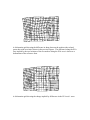
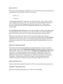
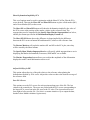
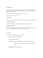
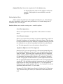
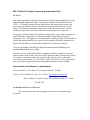
IMP: PCAGen6- Principal Components Generation Utility
PCAGen6
This software package is a Principal Components Analysis utility intended for use with
landmark based morphometric data. The program loads data in the IMP file format
(X1Y1…CS format) starting from any superposition and computes the partial warp
scores based on the data, using a GLS Procrustes mean specimen based on all data
loaded. The Principal components (eigenvectors of the covariance matrix) are then
calculated based on the covariance matrix derived from the partial warp scores.
The program will then display the landmark configurations, a plot of the data along any
pair of Principal components axes and the deformation implied by any Principal
component vector. All displays are color and symbol coded by group It is also possible to
plot the deformation implied by any pair of values along the Principal component axes
plotted, and the difference in deformation implied by two different positions.
If you are not familiar with IMP you should download and read WhatIsImp and
CoordGenManual before proceeding.
From time to time, all the IMP software is upgraded, and the recompiled versions are
made available on the website. The most recent compilation date is listed on the website
for each piece of software. Improved versions of the software will be coded with a
version letter after the name, ie. PCAGen6b would be the b level revision. This manual
may or may not be updated at the time the upgraded software becomes available.
Approximate User's Manual - in development
Conceptualization: H. D. Sheets, D.L. Swiderski and M.L. Zelditch
Coding, GUI and Software Design: H. .D. Sheets [email protected]
Dept. of Physics, Canisius College, 2001 Main St. Buffalo, NY 14208
716-888-2587
An Example of the Use of PCAGen
The example below shows the groupings of three species of piranha using
PCAGen6
An example of specimens (shown in Bookstein Coordinates) from three species for
piranha, coded by color and symbol.
06
04
02
0
02
04
-0.1
-0.08
-0.06
-0.04
-0.02
0
0.02
0.04
0.06
A scatter plot of the PCA axes scores of the specimens shown in the picture above. The
x-axis of this plot is the first PCA axis, explaining 51% of the variance, the y-axis is the
2nd PCA axis, explaining 16% of the variance. The same color coding of groups is used
in this figure as in the previous figure.
A deformation grid showing the difference in shape between the markers (the red and
green dots with cross-hairs) shown in the previous figures. The difference along the PCA
axes implied by the two locations of the two markers along the PCA axes is shown as a
deformation of the reference form.
A deformation grid showing the change implied by differences in the PCA axis 1 score.
Using PCAGen6A
Before starting to use PCAGen6, you need an input data file of morphometric landmark
data in X1Y1..CS format. If you are using multiple groups, all of the groups have to put
into a single file. Use Excel or a word processor to do this. Note that like all IMP
programs, PCAGen6 does not fully support data labels. However, if you add a percent
sign (%) followed by your label or comments at the end of each line of the data file, the
data files will load into all IMP software. The software will simply ignore the label.
If you want to color and symbol code different groups in your data set, you will also need
to prepare a Group Membership List File. This is an ASCII text file with the same
number of lines as there are specimens in your input data file, with a single number on
each line, specifying the color and symbol to use for that particular specimen. The best
way to produce this file is to load your input data file into Excel and to copy the group
code into a column at one end or the other of the data. Then copy this column (with codes
for each sample) into a new Excel worksheet. Note that you do not have to use a Group
List if you don’t want (or need) to, there is an option to bypass the group list, so that no
color coding of the data is done.
PCAGen6 is a handy way to identify outliers or errors in data files, since it can label the
PCA diagrams with specimen numbers. This is probably the quickest way to find errors
in data files. You don’t need to worry about a group list if this is all you want to use
PCAGen6 for.
Example File
Included in the self-extracting compressed data file for PCAGen6, is an example data set,
schizops.txt and a Group Membership List for this data set, schizogroup.txt. This data set
is the schizophrenic and normal brain data from Bookstein, "Biometrics, biomathematics
and the morphometric synthesis", and was obtained from the Morphometrics Website at
SUNY Stonybrook maintained by James Rohlf. The data set has been converted into the
X1Y1..CS data format, and Procrustes superposition and stored in the file schizops. The
first 14 specimens are "normal" brains, the last 14 are schizophrenic. The file
schizogroup.txt lists group membership codes of 1 for normal brains and 2 for
schizophrenic. This data set does not seem to be a particularly interesting data set as far
as using PCA analysis, but it does show how the program works.
Available Group Codes
There are currently 12 available color codes in PCAGen6. It may be possible to add
more, but it is hard to distinguish among 12 as it is. You may want to split the data into
subgroups if you have more than 12 groups. The available color and symbol codes are
Number
Color and Symbol
1
Black Circle
2
Blue x
3
Red star
4
Magenta square
5
Cyan +
6
Green *
7
Yellow Triangle
8
Black Triangle
9
Blue Circle
10
Red Square
11
Cyan Circle
12
Cyan Circle
Button-by-Button Guide to Using PCAGen6
Load File
This button loads a file. The file must be in X1Y1..CS format. It may be in any
superposition. The program will then display the name of the file loaded, the number of
specimens in the file and the number of landmarks on each specimen, in the file box
below the button.
No Group List
This button informs the software that you (the user) are not using a Group List with this
data set. When you hit this button the software will:
a.) Plot the data loaded onscreen.
b.) Compute a Procrustes GLS mean reference using all the data in the set.
(Note that there is now an option under the file menu that allows you to
enter a different reference, although this option must be used with care.)
c.) Compute the thin plate spline decomposition of the data, generating
partial warp and uniform component scores based on the computed
reference.
d.) Compute the variance-covariance matrix based on the partial warp and
uniform component scores of all the data.
e.) Compute the Principal components of the variance-covariance matrix,
the variance explained by each Principal Component and the Principal
Component Axis scores for each data point.
Be patient, this is a lot of calculations…..
Load Group Membership List
This button allows you to load the group membership list and then performs all the
calculations listed above in the description of the behavior of the No Group List button.
Show Landmarks:
Show Procrustes
Display the plot of the landmarks in Procrustes Superposition. The plot will be color
coded if you entered a Group Membership List.
Show BC
Display a plot of the data in Bookstein Coordinates, using the landmarks in the baseline
boxes below the button.
Show SBR
Display a plot of the data in SBR, using the landmarks in the baseline boxes below the
button.
Show PCA Plot
This option plots the Principal Component scores of all the data points along the Principal
components specified in the boxes below. The settings
X axis, pc 1
Y axis pc 2
would display the Principal component score along PC1 as the x-axis variable, and the
scores along the PC2 as the y-axis. You can use the UP and Down buttons next to each
box to select the Principal Components to display along each axis. The percent of
variance explained by each PC will be displayed in the box next next to the UP and
Down buttons.
The Label Points on PCA plot button will cause the Show PCA Plot to plot labels on the
PCA plot diagram when it is selected. To get rid of the labels, click on the Label Points
button again, then use the Show PCA Plot to replot the diagram without the labels.
The plot with the labels on it can be a bit busy with all the labels on it, making it
impossible to read the labels. There is a zoom function available under the Axis Controls
menu that will allow you to zoom in on the desired portion of the diagram, which will
allow you to read the labels. This is particularly helpful for finding outliers or errors in
data files.
Display PCA Deformation (BC)
This displays the deformation implied by the chosen Principal Component, using the
display format selected in the Deformation Display Format box located in the aqua box
on the left side of the screen. The box below the Display PCA Deformation (BC) button
selects the PC component displayed, chosen using the UP and DOWN buttons. The
scaling factor box sets the multiplier of the deformation in this display, since the PC
deformation is normalized to an amplitude of 1 during the calculation of the Principal
Components. The baseline used for the BC display is selected using the baseline
endpoints specified in the light green region on the upper right side of the screen.
Display Def (Procrustes)
Shows the deformation implied by the chosen PC score using a Procrustes superposition.
Display PCA Deformation (BC)
Show the deformation implied by the chosen PC score using SBR.
Show Deformation Implied by PCA
This set of options must be used in conjunction with the Show PCA Plot. Plot the PCA
scores desired. Then use the Place M1 and Place M2 buttons to place a Red marker (M1)
and a Green Marker (M2) on the screen.
The Show M1 and Show M2 buttons will show the deformation implied by the value of
the PCA scores at the position of the marker, relative to the reference form. The
superposition used is controlled by the Specify Show Marker Superposition box below,
and the plot format specified in the Deformation Display Format box.
The Show M2-M1 button shows the difference in shape implied by the difference
between the PCA scores at button M2 and button M1, relative to the reference form.
The Restore Markers will replot the markers M1 and M2 on the PCA plot, since they
will be erased by the Show buttons.
The Specify Show Marker Superposition box will specify which superposition to use in
displaying the Marker deformations, Procrustes, SBR and BC are available.
The Marker Exageration button allows you to adjust the amplitude of the deformation
displayed to make a small deformation easier to see.
Adjust Grid Size for PW
This option adjusts the size of the grid relative to the reference when plotting the
deformations implied by PCA scores. Adjust this value to achieve the desired coverage of
the reference form.
Save PCA Scores
This options saves the PCA scores for each specimen along rows of the file. The last
column is the centroid size. The scores are packed with the PCA scores corresponding to
the largest PCA scores last in the file, next to the CS value. The eigenvalues decrease
from right to left across the file. (Yes, this is a counter-intuitive way to output the data,
but that’s how Matlab calculates eigenvectors).
Save PW Scores
This option saves the partial warp plus uniform scores in a file, with the highest partial
warp scores appearing first in the file and the uniform components last, before the CS.
The format is shown below:
PW3X PW3Y PW2X PW2Y PW1X PW1Y UniX UniY CS
1.2 0.3 -0.3 0.1 2.1 -1.8 0.3 0.35 4.32
Save Reference
Save the reference form used in the PW score calculates to disk, for use in other software.
Copy Image to Clipboard
Copy the current image to the windows clipboard as an enhanced metafile.
Copy Image to EPS File
Copies the current image to an Encapsulate Post-Script file, which will load into Adobe
Illustrator, and perhaps other software that do not use the clipboard.
Axis Controls
This menu option has the following controls available
Remove Axis-removes the labeled axis.
Restore Axis-replots the axis.
Zoom On- allows a zoom in on the figure. Draw a box on the figure using
the mouse, the figure will zoom in. You can zoom repeatedly if
desired.
Zoom Off- turns off the Zoom function.
Original Plot Size- Restore the original plot. Do this before using
the Zoom Off option, otherwise the graphics can become
unstable. If the graphics becomes unstable, restart the
program.
Display Options Menu
Allows control of symbol sizes, lineweights and what have you. Some changes
take place immediately, others on the next plot function, so if a menu change has no
immediate effect, re-do the plot.
Statistics Menu -more statistics coming soon…watch for updates.
Scree Plot (eigenvalues)
Shows a scree plot of the raw eigenvalues of the variance-covariance
matrix.
Scree Plot (percentages)
Shows a scree plot of the percentage of variance explained by each of the
Principal Components as a percentage of the total variance. This plot may
be used to determine how many Principal Components should be used, the
rule of thumb is to use the last component before the Scree plot flattens
out. The other approach is to use the statistics discussed below.
Significant Differences in PCA components
Morrison (1967) gives an expression for a Chi-squared statistic that may
be calculated to determine if a pair of PC axis are significantly different
from one another. This menu option computes the pairwise comparison
statistic, starting with the 1 and 2 PC, then 2 and 3 and so on, until a pair
of components is not statistically different at 5%, using the Chi-square
statistic. The program will then indicate to you the highest numbered PC
that was still significantly different from the next PC. If the program tells
you that PC 3 was the highest numbered component that was significantly
different from the others, this means that PCs 1,2,3 are all statistically
different from one another and from PC 4,5,6…etc, but that PC 4 was not
significantly different from PC 5, and so forth.
See pages 221-254 of Multivariate Statistical Methods by D.F. Morrison,
1967, McGraw-Hill, QA276.m69, for a discussion of the statistical test
used.
Clear Data and Reset
This button clears the data and resets the software.
Exit
Exit.
File
This menu allows for several further options, and repeats some file I/O.
Save Principal Component Vector MatrixThis options saves the Principal Component vectors in Matrix form, with
the Principal Component corresponding to the smallest eigenvalue is in the
column on the leftmost side of the Matrix and the Principal Component
corresponding to the largest eigenvalue is in a column on the rightmost
side of the matrix. (The 1st Principal Component in the rightmost column).
The first row is the loadings on the highest numbered x component of the
Principal Warps, the 2nd row is the highest numbered Y component
Principal warp, the 3rd row is the second highest x component Principal
Warp and so forth. The last two rows are the loadings on the Uniform x
and Uniform y terms.
Save EigenvaluesThis saves a list of the eigenvalues, in the same sequence as the
eigenvectors above.
Load DataThis carries out the same function as the Load Data button.
Load ReferenceThis allows the user to load a reference form. The user reference must be
loaded after the data set, but before the group list. Most users will not
need this option, and it should be used with care.
Load Group ListReplicates the operation of the Load Group List Button.