1
Ultrasonic Measurement of
Thin Condensing Fluid Films
By
Michael A. Shear
A Thesis
Submitted to the Faculty
Of the
Worcester Polytechnic Institute
In partial Fulfillment of the Requirements for the
Degree of Master of Science
In
Electrical Engineering
April 18, 2002
APPROVED:
___________________________
Prof. Peder C. Pedersen, Advisor
___________________________
Prof. James C. Hermanson, Co-Advisor
___________________________
Prof. Fred J. Looft III, Committee Member
Abstract
The condensation of vapor onto a cooled surface is a phenomenon which
can be difficult to quantify spatially and as a function of time; this thesis describes
an ultrasonic system to measure this phenomenon. The theoretical basis for
obtaining condensate film thickness measurements, which can be used to
calculate growth rates and film surface features, from ultrasonic echoes will be
discussed and the hardware and software will be described. The ultrasonic
system utilizes a 5MHz planar piston transducer operated in pulse-echo mode to
measure the thickness of a fluid film on a cooled copper block over the fluid
thickness range of 50 microns to several centimeters; the signal processing
algorithms and software developed to carry out this task are described in detail.
The results of several experiments involving the measurement of both noncondensing and condensing films are given. In addition, numerical modeling of
specific condensate film geometries was performed to support the experimental
system; the results of modeling nonuniform fluid layers are discussed in the
context of the effect of such layers on the measurement system.
i
Acknowledgements
The financial support of NASA and the National Center for
Microgravity Research on Fluids and Combustion is gratefully
appreciated, as is the assistance of Dr. Jeff Allen, NASA/GRC project
liaison.
I would also like to thank Prof. Peder C. Pedersen, my thesis
advisor, for his endless help and encouragement throughout the
course of this project. His eternally optimistic and friendly attitude
somehow managed to turn this project from something that I had to
do into something that I wanted to do.
Prof. James C. Hermanson, the condensation project Principal
Investigator and my thesis co-advisor, along with his post-doctoral
fellow Dr. Zhenqian Chen, were extremely helpful in working with the
physical experiments and in teaching me enough about fluids to
understand why this project was important.
Finally, I would like to thank my family and friends, without
whose support I would never have managed to complete this project.
ii
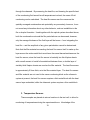
Extended Abstract/Summary
The mechanics and behavior of condensation phenomena are poorly
understood under even relatively commonplace conditions; in unusual conditions,
such as reduced gravity as experienced in the course of space flight, the
condensation process is expected to proceed differently and current theory may
not adequately predict condensation behavior in such a case. As a result the
National Aeronautics and Space Administration (NASA), through the Glenn
Research Center in Cleveland, Ohio, has funded a project to develop a lowgravity experiment to empirically determine the condensation dynamics of
assorted fluids in altered gravity conditions. The results of this research will be
valuable in designing future spacecraft to minimize concerns about water
condensation at unwanted locations and to enable better design of spacecraft
thermal control systems. In existing spacecraft, condensate management has
largely been an empirical art; this has for example resulted in modifications to the
International Space Station while in orbit when certain radiators had to have
insulation added to reduce unwanted – and unexpected – condensation
problems. Additionally, many thermal control devices such as heat pipes depend
on the high heat flux associated with the phase change occurring at
condensation.
The goal of this thesis project is the development of a pulse-echo
ultrasonic system to measure the thickness of a condensing film in real time, as
well as being able to post-process the data to determine wave velocity and
wavelength data for perturbations within the condensing film. This is done using
several (as many as eight in the current version) ultrasound transducers on the
outside surface of the condensation chamber. It is envisioned that in laboratory
iii
experiments the ultrasound system will be used with an optical imaging system
due to an optical system’s much better spatial resolution for imaging
perturbations in the film and the ultrasound system’s ability to perform
quantitative thickness measurements. In an actual low-gravity experiment, the
optical system may prove to be impractical and thus may be eliminated if the
laboratory experiments show the ultrasound system able to produce all needed
data.
This research was conducted using a condensation test cell. The cell
consists of a cylindrical shell constructed of relatively insulating plastic, with
several fittings for introducing vapor into the test cell, and one end of the cell
made of copper with cooling channels piped through it. The cell can be placed in
either “plate-down” or “plate-up” orientation on the benchtop; in the former case,
+1g conditions apply to the condensation and in the latter case a –1g effective
gravity level is present. An instrumented version of the test cell is scheduled to
be flown on NASA’s KC-135 low-gravity parabolic trajectory aircraft, permitting
experiments to be conducted in effective gravity levels ranging from 1g to 0.01g.
In operation, the end plate will be cooled by a refrigerant pumped through
the cooling channels. When heated vapor is introduced to the test cell, the vapor
will begin to condense onto the cooled plate. Monitoring the progress of this
condensation is no simple task as no direct measurements (e.g. using a float
gauge) can be made since they would disturb the condensation process. A
simple optical technique can image perturbations in a fluid film, but it is a
generally qualitative measurement. While the optical technique can determine
the presence of perturbations and their lateral characteristics, it cannot easily
determine film thickness or, for that matter, the depth of the perturbations on the
film. The need for accurate determination of condensate film thickness, as a
iv
function of time and at several locations, has motivated the development of the
ultrasound-based measurement system.
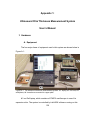
Eight ultrasonic transducers are connected through a multiplexer to a
pulser-receiver (P/R) unit; this P/R unit is then connected to a computer-based
oscilloscope which both triggers the P/R unit and records its output. The
oscilloscope hardware is entirely contained within a single Type II PCMCIA, or
laptop computer expansion, card; this card is inserted into one of the two Type II
PCMCIA expansion slots in the laptop and can then be treated as an integral part
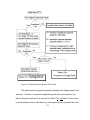
of the laptop itself. The oscilloscope is controlled through a control program
written in the National Instruments Inc. LabVIEW language; this program
performs all data processing as well as all control of the multiplexer as well as
the oscilloscope. The data from the P/R unit is processed through several signalprocessing steps, and the thickness estimate is extracted from this data. This
process is repeated for each of the active transducers (from one to eight
transducers can be used) and is continuously repeated to generate a thicknessvs-time record. The maximum sampling rate with multiple transducers is
approximately 30 samples/second (i.e. 15 samples/second/transducer for two
transducers, 10/second for three, etc.) or up to 60 samples/second with a single
transducer since the delay introduced by switching channels in the multiplexer is
removed. The multiplexer is also controlled by the LabVIEW program, and is
connected to the laptop using a standard serial interface.
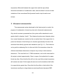
Condensate layers which are thin relative to the wavelength of the
ultrasonic signal have the frequency response of a “comb filter”; in other words,
the reflected energy due to a broadband ultrasound pulse falls in certain
v
narrowband frequency ranges. The center frequencies of the passbands of the
comb filter fulfill the equation (2n+1)fo where n is an integer greater than or equal
to zero and:
c
4d
(1)
c
4 fo
(2)
fo =
or, equivalently,
d=
where d is the thickness of the fluid layer in meters and c is the speed of sound in
the fluid in meters/second.
The f0 value is extracted through Fourier analysis of the signals acquired
by the system. If the fluid layer is of an appropriate thickness for this technique
to work (approximately 50-2000 microns) the FFT will have clear peaks at odd
multiples of f0 (f0, 3 f0, 5 f0, 7 f0, etc.) and the locations of these peaks are
extracted using a peak-detection algorithm which produces an estimated f0 and
thus through equation (2) the estimated layer thickness.
Due to the fact that the echo received by transducer from the copper/water
interface is much larger than the “comb-filtered” signal of interest from the fluid
layer, the signal must be normalized by subtracting the effect of the copper/water
interface echo before this analysis can be done. This normalization is
accomplished by subtracting the echo received from a fluid layer of sufficient
thickness to approximate an infinite layer from the raw received signal prior to
performing the FFT; this signal-processing step also eliminates effects from
structures within the copper block itself.
vi
For thicker layers, a more conventional echo-delay method is used. In this
method, the interval between the arrival time of the echo from the copper-fluid
interface and the arrival time of the echo from the fluid-vapor interface is
measured directly and yields a thickness estimate through:
d=
c ⋅t
2
(3)
This method works for layers which are at least one or two wavelengths
thick. For the 5MHz center frequency transducers used, this means that this
method becomes useful for fluid layers with a thickness of approximately 0.5mm
or greater. Tests to this point have demonstrated its use at up to 4cm of
thickness. Since the thin-film method becomes noisier above 750 microns and
the thick-film measurement is accurate above 500 microns, the system uses the
thick-film algorithm first, and if an invalid result or a result less than 750 microns
is generated, the thin-film algorithm is then run with the same data.
Numerical modeling using the Wave2000 software package has also been
performed; this software models the wave propagation in a 2-D object from a 2-D
transducer (the third dimension is assumed infinite). The Wave2000 system is a
finite time difference modeling system which models a 2-D object as a matrix of
points; the pressure at each point at a given time is used to calculate the
pressure at each adjoining point at the next time interval.
The simulation package was first used to model simple situations such as
a flat film, which was used to verify that the model was in good agreement with
the same experiment run in the lab. It was then used to investigate situations
vii
which would be very difficult to create experimentally under controlled conditions,
such as a thin film which varied in thickness or layers with droplet formation.
Experiments thus far have verified the validity of the results from the
ultrasound system; this has been done using a level block with the transducers
on the bottom surface and a fluid film on the top (i.e. a “+1g” environment). Both
static and dynamic – i.e. excited by some external mechanical activity – fluid
films have been used; the excitations have ranged from a slow, steady addition
of fluid to a dropwise addition of fluid resulting in ripples to waves generated by a
paddle.
In the initial set of experiments, static films of non-condensing fluid with
different thicknesses were used. This verified the system’s ability to detect a fluid
layer and accurately measure its thickness. The film thicknesses were measured
correctly by the system as far as could be verified although verification by nonultrasound means proved difficult for some of the thinner layers.
In the next set of experiments, the measurement began with an extremely
thin fluid layer to which fluid was added at a constant rate. Since the fluid was
added at a constant rate, the growth rate of the fluid was known to be constant.
The constant growth rate was directly verifiable and indeed is what was
measured by the system.
In the excited layer experiments, thickness-vs-time plots from multiple
transducers were used to calculate the wave velocity and the wavelength for
several different fluids at several layer thicknesses
Finally, a series of measurements of actual condensation have been
conducted. These tests have shown that the ultrasonic system developed for
this project can successfully monitor condensation in benchtop experiments.
viii
Table Of Contents
Abstract………………………………………………………………………..……....i
Acknowledgements…………………………………………………………..…...….ii
Extended Abstract……………………………………………………………..……..iii
Table of Contents…………………………………………………………………..…ix
Table of Figures………………………………………………………………..……..xiii
Table of Tables…………………………………………………………………..……xvii
I: Introduction……………………………………………………………………..….1
A. Background for Condensation………………………………………..…1
B. Measurement of Condensation………………………………………....7
C. Development Stages of the Proposed Measurement System……….8
D. Thesis Goals………………………………………………………..…….9
E. Thesis Outline………………………………………………………..……10
II: Condensation Test Cell Construction and Instrumentation………………..…13
A. Test Cell Mechanical Configuration…………………………………….13
1. Structural Configuration………………………………………….13
2. Cooling System ..…………………………………………………14
3. Vapor Introduction System………………………………………15
B. Non-Ultrasonic Instrumentation…………………………………………16
1. Optical System……………………………………………………16
2. Heat Flux Sensor…………………………………………………18
3. Temperature Sensors……………………………………………19
C. Ultrasonic Instrumentation……………………………………………….20
III: Acoustic Theory ………………………………………………………………….22
A: Pertinent Aspects of Ultrasonic Wave Theory …………………………22
1. Ultrasonic wave propagation theory…………………………….22
a. In a homogenous material……………………………….22
b. At an interface between materials………………………28
ix
2. Transducer and Excitation Theory……………………………..30
3. Characteristics of materials used………………………………31
B: Theoretical basis of film thickness estimates …………………………33
1. General Overview……………………………………………….33
2. Thin Layers: Frequency Domain……………………………...34
3. Thick Layers: Time Domain……………………………………42
4. Effects of deviation from parallel-surfaced film………………47
IV: Signal Processing and Algorithms…………………………………………….48
A. Overview………………………………………………………………...48
1. LabVIEW Control Program…………………………………….49
2. Signal Processing Common to Both Domains…………...….51
B. Time Domain…………………………………………………………….54
1.
Detection of ∆t and Calculation of Layer Thickness……….54
2.
Limitations of Time-Domain Method…………………………56
C. Frequency Domain…………………………………………………….58
1. Additional Signal Processing………………………………….58
2. Detection of fo and Calculation of Layer Thickness……..….61
3. Limitations of Frequency-Domain Method…………………..63
D. Additional Topics………………………………………………………65
1.
Transducer Excitation………………………………………..65
2.
Signal Averaging ...…………………………………………..67
V: Modeling ………………………………………………………………………..68
A: Introduction……………………………………………………………..68
1. Goals for modeling experiments………………………………68
2. Modeling software – Wave2000………………………………69
B: Modeling theory used in Wave2000………………………………….70
1. Equations Used…………………………………………………70
2. Explanation of Modeling Parameters…………………………71
a. Temporal ………………………………………………..72
b. Spatial……………………………………………………73
x
c. Material Parameters…………………………………..76
C: Model Setup……………………………………………………………77
1. Time Domain (Thick film)……………………………………..77
2. Frequency Domain (Thin film)………………………………..81
3. Non-uniform-thickness films………………………………….82
VI: Experimental Work……………………………………………………………86
A: Experimental System…………………………………………………..86
1. Overall Systems Description…………………………………..86
2. Hardware………………………………………………………..88
a. Laptop…………………………………………………..88
i.
System Description……………………………88
ii. Operating system……………………………..89
i. LabVIEW software…………………………….89
ii. Oscilloscope card……………………………..90
b. Pulser-Receiver……………………………………….91
c. Multiplexer……………………………………………..92
d. Transducers……………………………………………94
3. Software…………………………………………………………96
B: Experimental Setup……………………………………………………………100
1. Stationary (non-excited).……………………………………..100
2. Slow constant layer growth…………………………………..102
3. Excited layers………………………………………………….103
4. Condensation………………………………………………….107
VII: Results………………………………………………………………………..109
A: Physical Experiment Results…………………………………………109
1. Stationary (non-excited) experiments………………………..110
2. Slow constant layer growth experiments…………………….111
3. Excited layer experiments…………………………………….114
4. Condensation Experiments…………………………………..118
B: Numerical Modeling Results………………………………………….124
xi
1. Model Verification……………………………………………….124
2. Numerical Modeling of Complex Layer Geometries………...128
VII: Conclusions…………………………………………………………………….135
A. Evaluation of the Ultrasonic Film Measurement System……………135
B. Suggested Further Research / Development in this area…………..136
References ..…………………………………………………………………………138
Appendix A: System User’s Manual………………………………………………139
Appendix B: System Technical Manual…………………………………………..148
xii
Table Of Figures
Figure 2-1:
Schematic cross-sectional view of the condensation test cell…14
Figure 2-2:
A schematic representation of the optical monitoring system…17
Figure 2-3:
Optical System Physics…………………………………………….18
Figure 3-1:
Defining the Regions of a Simple Fluid Layer……………………35
Figure 3-2:
Model of thin-film (frequency domain) system behavior………..36
Figure 3-3:
The Magnitude of the Frequency Response of a 0.2mm
Water Layer…………………………………………………………39
Figure 3-4:
Normalized Analytically Predicted Received Signal for a
0.2mm water layer with a 5MHz center frequency transducer
excited by a 5MHz ½ cycle square wave…………………………40
Figure 3-5:
Normalized Analytically Predicted Received Signal for a
0.5mm water layer with a 5MHz center frequency transducer
excited by a 5MHz ½ cycle square wave…………………………41
Figure 4-1:
Basic Conceptual Model of Ultrasonic Fluid Layer
Thickness Measurement System………………………………….48
xiii
Figure 4-2:
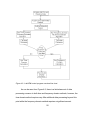
LabVIEW control program overview flow chart…………………..50
Figure 4-3:
Extraction of the Desired Portion of the Signal…………………..53
Figure 4-4:
Frequency-Domain Algorithm Additional Signal Processing……58
Figure 4-5:
Peak-Detection Algorithm Flow Chart……………………………..61
Figure 4-6:
An Evaluation of an Untuned Pulser-Receiver vs Different
Tuneable Pulser-Receiver Settings for a 0.75mm Water Film….66
Figure 5-1:
An image of a typical time-domain simulation geometry………..78
Figure 5-2:
The excitation signal sent by the transducer in the Wave2000
model………………………………………………………………….79
Figure 5-3:
Run-time parameters used for Time-Domain models……………80
Figure 5-4:
An image of a typical frequency-domain simulation geometry…82
Figure 5-5:
An image of a non-uniform film geometry…………………………83
Figure 5-6:
Two droplet models………………………………………………….84
Figure 6-1:
A block diagram of the ultrasonic thickness measurement
system…………………………………………………………………86
xiv
Figure 6-2:
Digitizer card connector cable………………………………………90
Figure 6-3:
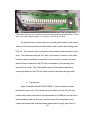
34903A Actuator/General Purpose Switching card………………94
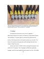
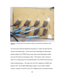
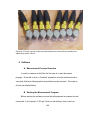
Figure 6-4:
Eight transducers mounted to the copper block………………….96
Figure 6-5:
A simple example “G” program…………………………………….97
Figure 6-6:
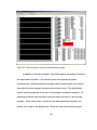
The front panel of the main measurement program……………..99
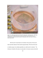
Figure 6-7:
Initial experimental test block with Tupperware “swimming
pool”…………………………………………………………………..101
Figure 6-8:
Second experimental test block with polyethylene rim………….105
Figure 7-1:
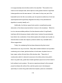
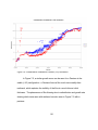
Data from a constant-layer-growth trial………..………………….112
Figure 7-2:
Linearly Growing Film Thickness …………………………….……114
Figure 7-3:
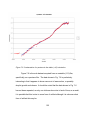
Data used to generate velocity and wavelength
measurements for paddle-excited layers of ethylene glycol……118
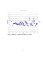
Figure 7-4:
Condensation of Methanol in Stable (+1G) configuration..……..121
Figure 7-5:
Condensation of n-pentane in Stable (+1G) orientation….…….122
Figure 7-6:
Condensation of n-pentane in Unstable (-1G) orientation………123
xv
Figure 7-7:
Normalized Model output for a simulated 0.1mm water layer..…125
Figure 7-8:
Spectrum of 0.1mm Water Layer Model Output………………….126
Figure 7-9:
Model Output for a Simulated 0.5mm water layer………………..128
Figure 7-10: The spectrum of a 0.3mm (center thickness) water layer, with
40% center-of-beam to edge-of-beam (3mm radius) thickness
difference……………………………………………………………..130
Figure 7-11: Effect of a 1.5mm diameter droplet on the measurement of a
1.0mm water layer………………………………………………...…132
Figure 7-12: Spectra of repeated 0.1mm radius droplets on bare copper…..134
xvi
Table Of Tables
Table 3-1: Material Properties of Solids……………………………32
Table 3-2: Material Properties of Liquids…………………………..32
Table 3-3: Material Properties of Vapors at Room Temperature..33
Table 7-1: Results of Ethylene Glycol Experiments:
wavelengths and velocities resulting from
paddle motion………..……………………………………117
Table 7-2: Results of Thin Layer Simulations………………………127
xvii
Chapter 1: Introduction
A. Background for Condensation
This thesis deals with an ultrasound-based method for measuring the
thickness of a thin film of condensing fluid. It is thus pertinent to begin with a
brief description of condensation dynamics.
Under normal conditions, matter is found in one of three phases listed
here in order of increasing internal energy: solid, in which molecules are rigidly
attached to each other; liquid, in which molecules are loosely and fluidly bound
together; and gaseous, in which very little intermolecular bonding is present.
When a substance changes from one phase to another, internal energy (or
“enthalpy”) must be added or removed by an external source; for example, in
order to boil water to create steam, heat must be added by a burner or other heat
source. More pertinently, when water vapor condenses into liquid water, the heat
released by the condensation phase change must be removed; in an everyday
example, water vapor from the air condensing onto a glass of a cold beverage
transmits the heat from the phase change through the glass into the cold
beverage.
1
This process is, however, complex. In the example above of
condensation onto a glass, the condensation dynamics are affected by many
parameters. Some of these are: the partial pressure and temperature of the
water vapor; the initial temperature, thermal conductivity, and thermal capacity of
the glass; the temperature, thermal conductivity, and thermal capacity of the
liquid in the glass; the orientation of the condensing surface; the velocity of
airflow past the glass; and the viscosity and thermal conductivity of the
condensate.
The ambient water vapor, being intermixed with the ambient air, circulates
with that air and is cooled by the liquid water layer on the glass. When a
molecule of water vapor has been sufficiently cooled, it experiences a phase
change to liquid thus adding to the liquid water layer. The circulation of the
ambient air, which brings the water vapor in contact with the liquid water layer, is
in part due to the convection caused by the cooling effect of the glass.
Convection, as will be discussed below, is a gravity-driven process.
When a water molecule condenses from the ambient water vapor to join
the liquid water layer, the enthalpy of phase change (approximately 2.5x10⁶ J/Kg
for water) is released. This heat is deposited into the liquid water layer on the
outside of the glass, from where it is removed by heat conduction through the
liquid layer (assuming that the layer is thin enough to prevent convection). For
fluids significantly thicker than usually found in terrestrial situations, convection
would be expected to play a role in this process as well. The heat is then
2
transferred through the solid glass layer by the mechanism of conduction, which
is independent of gravity.
Heat is transferred from the inner wall of the glass to the beverage through
the mechanism of convection, which is often the predominant mechanism of heat
transfer in liquids and gasses. Convection is a gravity-driven process in which
the fluid circulates because of the different densities of cold and warm fluid. In
most fluids, warming the fluid causes it to expand, and thus become less dense;
having become less dense, the warmer fluid tends to rise and be replaced by
colder and thus denser fluid. This mechanism distributes added heat throughout
the body of the fluid, minimizing the amount of heat absorbed by any particular
portion of the fluid. Convection also applies to heat loss, in that the fluid that has
lost heat will become denser and thus sink and be replaced by warmer and less
dense fluid.
Of the four regions discussed in the example of a glass filled with a cold
beverage, two have behaviors which are dependent on gravity: the air/water
vapor mixture and the beverage in the glass. However, if the condensate film
were to grow thick enough, convection would be expected to play a part in that
region as well. In an environment without gravity, convection will not occur. It is
theorized that this will significantly slow heat transfer which normally occurs
convectively, as it will now be limited to heat conduction instead which implies a
much lower rate of heat transfer. This means that, for example, the air/water
vapor mixture will not move past the surface due to natural convection;
3
implications of this could be a significant slowing of the condensation process
due to less water vapor being present immediately adjacent to the condensing
surface. Additionally, the fluid mechanics of all three non-solids in this example
will be significantly altered by the absence of gravity.
While the condensation onto a glass of a cold beverage in a reduced
gravity environment may not be very important, the reduced gravity behavior of
cooling systems that exploit the same physical phenomena is critically important.
As a result, the National Aeronautics and Space Administration (NASA), through
the National Center for Microgravity Research on Fluids and Combustion at
Glenn Research Center in Cleveland, Ohio, has funded research into
condensation physics in reduced-gravity environments.
Condensation behavior is an important factor in the design of spacecraft
systems such as air circulation and atmospheric water recovery systems based
on condensation. Among other functions, these systems ensure that cabin air in
spacecraft is at an appropriate humidity level for both crew and equipment. To
do this, a device similar to a household dehumidifier condenses excess
atmospheric water vapor to remove it from the air.
Additionally, condensation is a critical part of certain thermal control
systems, which utilize the high heat flux from the phase change as an important
part of their function. A phase change of water between liquid and gaseous, or
vice versa, involves a heat flux of approximately 2.5x10⁶ Joules per kilogram of
water; the same kilogram of water would have to be heated or cooled several
4
hundreds of °C – assuming it could be kept liquid – to accommodate the same
heat flux without a phase change. An example of such a component using this
high heat flux would be “heat pipes”; these are passive heat transport devices
which are commonly used in spacecraft. A heat pipe consists of a sealed metal
tube, with a wick on the inner surface of the tube, containing a working fluid with
a high enthalpy of vaporization (examples are water, methanol, and ammonia).
Because of the physics of the phase change, thermal energy is absorbed by
changing the working fluid from liquid to gas with no change in temperature since
the phase change is an isothermal process; this means that the entire heat pipe
will always be at the boiling point of the working fluid at the pressure in the tube.
Energy released from the working fluid changing from gas to liquid is transmitted
out of the heat pipe to a radiator or other heat sink, still at the same boiling point
temperature. The name “heat pipe” refers to the phenomenon that the heat is
transferred from one end to the other at a constant temperature.
When one end of the heat pipe is heated and the other cooled, for
example by attaching one end to an electronics rack and the other to a radiator,
heat energy at the hot end is used to change the phase of the working fluid from
liquid to vapor at a constant temperature. The vapor travels down the tube, and
upon reaching the cold end condenses onto the end plate releasing the enthalpy
of vaporization that it absorbed at the hot end. The pressure differential created
by vaporization at the hot end and condensation at the cold end acts as a
passive pump for the vapor; the wick built into the tube passively transports the
5
liquid phase back from the cold end to the hot end. No active parts are required,
and the passive components are extremely simple, and as a result these devices
are very reliable; this is, of course, important for spacecraft applications.
However, in terrestrial applications the heat transfer occurring between the
end plate and the fluid at both the hot end and the cold end is by the mechanism
of convection; in a reduced gravity environment, it would take place solely by
conduction. Heat pipes have been used extensively in spacecraft design, but the
fundamental physics of their operation in reduced gravity is not well understood.
Various aspects of the fundamentals of condensation have been studied
many times under terrestrial conditions. However, the terrestrial mechanism of
condensation is highly complex; thus, the implications of a reduced gravity
environment on the condensation phenomenon are poorly understood and
cannot be inferred from current data. The reverse process from that of
condensation is boiling, which has been studied extensively in microgravity
conditions. However, the fundamental fluid physics of condensation in
microgravity have not been investigated; although the two are inverse processes,
the results from pool boiling experiments cannot be used to infer condensation
behavior.
A series of condensation experiments is planned in order to explore the
phenomenon of condensation in reduced gravity. However, the approach to
measuring condensation as it progresses is not obvious. The subject of this
6
thesis is a monitoring system to measure the progress of condensation in this
test cell, which is intended for use in reduced-gravity experiments.
B. Measurement of Condensation
Several methods of measurement of condensation experiments have been
considered, and the ones used in the current project are briefly described here.
A more thorough description is given in Chapter 2, which covers the
condensation test cell and its instrumentation.
One technique for measuring condensation is in the form of an optical
system which illuminates the condensate layer with a light source and projects
the reflections off of the fluid layer onto a screen where it is recorded with a video
camera. This system measures the topology of the fluid layer, but not its
thickness or growth rate.
A second approach to condensation measurement utilizes heat flux
measurements; if the temperature of the vapor is known, and the temperature of
the block onto which the vapor is condensing is known, the amount of fluid
condensing can be calculated from the total heat flux of the system. This
measures the condensation rate, but provides no information about the topology
of the fluid film nor about the film thickness at any given time.
7
The third measurement system used to monitor the progress of
condensation in the current experiments is an ultrasonic system. This system is
the subject of this thesis, and as such will be described in much greater detail in
later chapters. The ultrasound system uses several transducers in pulse-echo
mode to determine the thickness of the fluid film in discrete locations opposite
each transducer. This can yield limited topographic information as well as
thickness and growth rate information.
C. Development Stages of the Proposed Measurement System
The ultimate goal of this research will be the ability to perform meaningful
study of condensation in reduced gravity. However, many aspects of the fluid
physics of condensation take place over too long of a time frame to be studied in
short periods (less than several minutes) of microgravity. These aspects of
condensation can only be fully studied in a spaceflight experiment to be flown on
the Space Shuttle or the International Space Station. It is hoped that the
systems developed for the current project can be used in a modified form for
such spaceflight experiments. However, the goals of the current project are
more modest: a system will be developed to perform condensation research on
NASA’s KC-135 parabolic trajectory aircraft which provides a reduced-gravity
environment in 20-25 second periods.
8
Before the KC-135 flights can take place, a condensation test cell and
measurement systems to monitor condensation progress within the test cell must
be developed. This was begun using a series of benchtop tests in the laboratory.
These tests will be discussed in detail in a later section of this thesis, but in
general consisted of using the ultrasound system to first measure noncondensing films of various fluids in both static fluid films and fluid films excited
by external stimuli. These benchtop tests were designed to validate the optical
and ultrasonic measurement systems.
Once these measurement systems were validated, benchtop
condensation experiments were carried out. These were performed in two
orientations: +1g (fluid condensing on the bottom of the test cell) and –1g (fluid
condensing on the top of the test cell). These experiments have further validated
the measurement systems, including the heat flux sensor system, and also
provide a baseline data set for comparison to reduced-gravity trials.
After benchtop condensation experiments have been successfully
accomplished, planning will begin for the KC-135 reduced-gravity flight
experiments. These experiments are anticipated to occur in the summer of 2003.
D. Thesis Goals
The main goal for this thesis project is the development, construction, and
performance evaluation of an ultrasonic system for the dynamic measurement of
9
condensation film thickness. As of the writing of this document, this system has
been developed and is functional, and evaluation with actual condensation is
ongoing. A secondary goal is to test this system, and verify its performance
experimentally. The system has been tested with several different fluids, with
both static and wavy fluid films, and with a wide range of fluid film thicknesses.
Finally, numerical simulations of the ultrasound interactions with the fluid film
have been carried out and used to verify the behavior of the system in situations
not easily created experimentally, such as droplet formation. This goal was also
fulfilled, as the system has been tested with simulations of nonuniform layers of
different thicknesses and shapes.
E. Thesis Outline
This thesis is structured as follows:
In Chapter 1, a general introduction to the thesis project and the larger
project of which it is a part is given. The motivation for both the overall
condensation research project and the ultrasound thesis project itself is
explained.
Chapter 2 describes the design of the condensation test cell, including the
mechanical construction of the cell, the functionality of the cell, and the
instrumentation installed in and on the test cell.
10
Chapter 3 explains basic ultrasonic theory pertaining to this project.
Included are such topics as general ultrasonic wave propagation theory,
descriptions of the ultrasound transducers used for the measurements and
transducer theory, and characteristics of the materials used in the condensing
block and fluid films.
Chapter 4 discusses all signal processing steps used in the course of the
project. This includes data extraction from the raw signals, algorithms for
generating a film thickness from the processed signal, and a flow chart of the
ultrasonic measurement software.
The numerical modeling of the ultrasound wave propagation carried out
for this project is discussed in Chapter 5. An overview of the modeling software
used is given, followed by a detailed discussion of modeling parameters used
and modeling techniques. Details of each modeled scenario are given, along
with details of the modeling parameters used.
In Chapter 6, detailed descriptions of the ultrasound measurement system
and experimental tests are provided. The chapter begins with an overall system
explanation, which is then followed by a detailed explanation of each segment of
11
the system including both hardware and software. The experimental setup is
then discussed, for each of several experimental scenarios.
The results of all experimentation along with all modeling results are given
in Chapter 7. The results of each experimental and modeling scenario are given,
along with a brief summary of the scenario conditions and parameters. The
experimental results are compared to the modeling results as well as to results
from other measurement systems (optical and heat transfer) furnished by the
Mechanical Engineering team.
Finally, Chapter 8 is a conclusion that addresses the question of whether
this thesis was successful in producing a satisfactory ultrasonic fluid layer
measurement system and suggests areas for further research.
12
Chapter 2: Condensation Test Cell Construction and
Instrumentation
A. Test Cell Mechanical Configuration
1. Structural Configuration
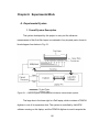
The basic structure of the condensation test cell is that of a cylinder with
thermally insulating plastic walls. The end of the cylinder at which condensation
occurs is made of copper and contains a cooling system and several types of
instrumentation; the other end is simply an optically clear layer of glass. The test
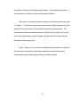
cell is shown schematically in Figure 2-1. A clamping mechanism, consisting of
a round metal plate at each end of the system bolted together via four threaded
rods, holds the system together; the center of each plate is milled out, making
each a ring, to allow for the placement of ultrasound transducers on one end and
light transmission on the other.
13
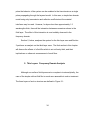
Figure 2-1: Schematic cross-sectional view of the condensation test cell. Note that for
clarity, portions of the right threaded rod are not shown.
2. Cooling System
Several fluid channels are drilled through the copper block, as shown in
Fig. 2-1. Chilled water is pumped from a Cole-Parmer “Polystat” chiller/pump unit
through these channels to allow the block to be cooled to the desired
temperature. The cooling channels are drilled with 1” (25.4mm) center to center
14
spacing and ½” (12.7mm) diameter, resulting in a ½” (12.7mm) space between
each adjacent pair of channels.
3. Vapor Introduction System
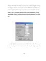
A vapor generator (not shown in Fig. 2-1) has been constructed which
allows the heating of the desired fluid to a controlled temperature to create a
specified partial vapor pressure. The vapor generator consists of a glass cylinder
which is sealed on the bottom and has a metal top containing instrumentation to
measure pressure and temperature and a fitting to connect to the pipe which
carries the vapor to the condensation cell. Electrical heating coils are wrapped
around the outside of the glass cylinder, and a thermocouple to sense
temperature is installed in the top to measure the temperature of the vapor
generated. The output of this thermocouple is sent to a heater control unit which
regulates the current through the heating coils so that a constant set vapor
temperature is maintained. A pressure gauge is also attached to monitor
pressure inside the vapor generator; when the desired pressure has been
reached, a valve is opened allowing the vapor into an insulated ½” copper pipe
leading to the condensation cell.
15
B. Non-Ultrasonic Instrumentation
1. Optical System
The optical monitoring system used in this project is the conceptually
simplest method to observe the progress of condensation, which is to simply
record a visual image of the fluid film as a movie. In practice, difficulties arise
since in the “double-pass shadowgraph” system used one is observing a
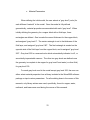
transparent fluid film at normal incidence. As shown in Fig. 2-2, the optical
system consists of an arc lamp shining through a partially silvered mirror and
reflecting off of a concave mirror onto the condensing surface which has been
polished to a high degree of reflectivity. The light is then reflected back onto the
concave mirror from where the light is directed towards the partially silvered
mirror, which reflects it onto a screen where it is captured by a video camera.
This method works well for recording perturbations in the fluid film, such as
waves and droplets, but is not capable of determining the depth of the film.
Because one of the main goals of this condensation research is to determine
condensation rate, knowing the fluid film thickness is critical; thus, the optical
method alone is an inadequate measurement methodology. However, the optical
method is potentially a valuable adjunct to other methods since it can in principle
detect disturbances in the fluid film and measure their size, shape, location,
wavelength, and velocity with high precision despite being unable to determine
16
their amplitude. The optical system has not performed as well as hoped to date,
and if the ultrasound system can acquire all needed topographic data the optical
system would not be needed for the reduced gravity experiments.
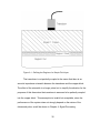
Figure 2-2: A schematic representation of the optical monitoring system.
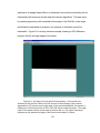
The physics of how this system works optically are shown in Fig. 2-3. A
thicker portion of the layer, such as a droplet, acts as a convex mirror and
reflects light away from a direct reflection resulting in a dark area on the display
screen. In contrast, a thinner portion, such as the trough of a wave, acts as a
concave mirror which focuses light creating a bright area on the screen. In both
Fig. 2-2 and Fig. 2-3, only two rays are shown in each figure to illustrate the
17
concept. The case shown in Fig. 2-3 is an ideal case, where the focal distance of
the trough is exactly the distance to the screen resulting in a perfectly focused
image. However, since waves vary in size and shape this is not usually the case.
Figure 2-3: Optical System Physics. Left: convex wave (peak); Right: concave
wave (trough).
2. Heat Flux Sensor
A second technique for monitoring the progress of condensation is to
measure the heat flux through the condensing surface. The condensing surface
is cooled by circulating a chilled fluid through cooling channels, and a heat flux
sensor is placed between these cooling passages and the condensing surface.
When condensation occurs, the heat released by the phase change travels from
the condensing surface through the copper block with high thermal conductivity
and through the heat flux sensor to the region of the block with the cooling
channels. The heat is then removed by the chilled water which is circulating
18
through the channels. By measuring the heat flux, and knowing the specific heat
of the condensing fluid as well as all temperatures involved, the mass of fluid
condensing can be calculated. The heat flux sensor can thus measure the
spatially averaged condensation rate potentially very accurately; however, it can
not reveal any information about any other behavior, such as instabilities in the
film or droplet formation. Used together with the optical system described above,
both the condensation rate and the film perturbations can be sensed; however,
only the average thickness of the fluid layer will be known – from integrating the
heat flux – and the amplitude of any given perturbation cannot be determined.
Note that the filler material surrounding the heat flux sensor itself to make up the
layer across the entire metal block must have the same thermal resistance as the
heat flux sensor; since the heat flux sensor is basically two thin Kapton sheets
with a small amount of metal foil sandwiched between them, a double layer of
similarly thick Kapton sheets are used as the filler material. The heat flux sensor
is approximately 0.2mm thick, as is the filler material layer. The heat flux sensor
and filler material are not used in the same condensing block as the ultrasonic
system at present; the heat flux sensor requires a thick metal block with the heat
sensor layer embedded, while the ultrasonic system requires a thin metal block.
3. Temperature Sensors
Thermocouples are placed at various locations in the test cell, to allow for
monitoring of temperatures during the experimental runs. Knowledge of the
19
temperature differential between the copper block and the vapor allows
theoretical calculations of condensation rates, and also allows for more accurate
calculation of the conventional fluid dynamics found in drop formation and
release.
C. Ultrasonic Instrumentation
The measurement system developed in this thesis project to monitor the
progress of condensation is based on pulse-echo ultrasound measurements.
Only a brief overview is presented here; this system will be described in much
greater detail in chapters 4 and 6. The ultrasound system uses ultrasonic pulses
from several transducers mounted on the non-wetted face of the copper block to
probe the thickness of the fluid layer at a location approximately the size of the
transducer face directly opposite each transducer (see Fig. 2-1). This holds true
as long as the condensing film is in the near field of the transducer, where the
effective lateral beam dimensions correspond very closely to the transducer
dimensions. The near field for a ¼” 5MHz transducer, such as the ones used for
this project, extends approximately 10mm in copper; this implies that for copper
blocks less than 10mm thick the film will be in the near field and each transducer
will measure an area of fluid roughly the same size as the transducer itself while
for copper blocks greater than 10mm thick the film will be in the far-field of the
transducers resulting in a larger beam area and significantly decreased SNR.
20
The system operates in pulse-echo mode, meaning that the piezoelectric
transducer which produced the transmitted pulse also receives the echoes from
the emitted pulse and converts them to a voltage output, allowing for a single
transducer to be used for each point where layer thickness is measured. The
great advantage of the ultrasonic system over the optical and heat transfer
measurement methodologies is that the fluid layer thickness can be measured
directly. The main advantage of the optical system is that it can image the entire
surface of the fluid film while thickness can only be measured ultrasonically at
discrete points. However, since the data from the ultrasound system is in digital
form it is easily stored; the optical data must be recorded using a video camera
which severely limits the performance of the optical system.
21
Chapter 3: Acoustic Theory
A. Pertinent Aspects of Ultrasonic Wave Theory
1. Ultrasonic Wave Propagation Theory
a. Propagation In a Homogeneous Material
An ultrasonic wave field emitted by a planar piston transducer, such as
those used in this project, presents a complex analytical situation due mostly to
diffraction effects. To greatly simplify the mathematical treatment of the wave
field, it will be analyzed based on a single plane wave assumption; this means
that the actual wave field is approximated as an infinite plane moving in a
direction normal to the plane. All signals which will be discussed in this chapter
will be treated as plane waves.
The representation of an ultrasonic wave in this chapter will be an
equation describing the acoustic pressure as a function of axial location and time.
The equation for the initial pulse emitted by the transducer is given as (3-1),
where the actual form of the pulse is not specified but is expressed as the timevarying pressure at a given location x=0.
p (t ,0) = p (t , x) | x=0
22
(3-1)
The coordinate system can be selected such that the plane of the wave is
the yz plane, and thus since the plane wave moves in a direction normal to the
plane of the wavefront all motion of the wave is along the x-axis. The origin is
chosen such that x=0 at the face of the transducer. Since the wave is a plane
wave traveling along the x-axis with velocity c, no amplitude or waveform
changes will occur if attenuation is neglected and p(t,x) can be represented by a
time shifted version of (3-1), given here as (3-2):
x
p(t , x) = p t − ,0
c
(3-2)
x
p(t , x) = p(t ,0) ⋅ δ t −
c
(3-3)
which can be written as:
The wave described in (3-3) moves with a velocity c in the +x direction,
with waveform p(t,0).
Thus far, all discussion has been in the time domain. It is, however,
pertinent to set the framework for a frequency-domain analysis since the thin-film
resonant layer system is analyzed in the frequency domain. Additionally,
attenuation is a frequency-dependent phenomenon which can be most
accurately addressed in the frequency domain. The frequency domain
23
representation P(ω,t) is defined as the Fourier transform of the time domain pulse
p(x,t) as in (3-4):
P (ω , x) = ℑ{p (t , x)}
(3-4)
P(ω ,0) = ℑ{p (t ,0)}
(3-5)
where
Referring to (3-2), (3-4) can be rewritten as (3-6):
x
P(ω , x) = ℑ p(t ,0) ⋅ δ t −
c
(3-6)
which can be evaluated to (3-7):
P (ω , x) = P (ω ,0) ⋅ e
− j⋅ω ⋅
x
c
(3-7)
Noting that the wave number k is defined by k=ω/c, (3-7) can be rewritten as (38):
P(ω , x) = P(ω ,0) ⋅ e − j⋅k ⋅x
24
(3-8)
In the ideal case, (3-8) would accurately describe the propagation of an
ultrasonic signal through a medium. However, there are two major non-ideal
conditions seen in the situations analyzed for this project. The first condition is
that the assumption of lossless media is invalid for any real medium; since both
the condensate fluid and copper are real and thus attenuating media the
assumption of lossless media is not technically valid. Water and the other fluids
used have very low attenuation and thus can be approximated as lossless for the
frequencies and thicknesses encountered in this project. Copper, however, has
significant attenuation which must be taken into account. The second condition
is that in addition to attenuation through the classical mechanisms of shear
viscosity and thermal conductivity, copper exhibits a grain scattering effect. The
former effect can be calculated and incorporated in theoretical analysis; the latter
exhibits macroscopic effects which are unpredictable. These effects can be
modeled once measured, but are different for each possible transducer
placement on a given block and of course differ from block to block as well.
However, the signal processing discussed in Chapter 4 will essentially eliminate
the effects of grain scattering so its absence from the theoretical discussion will
not be significant.
The standard attenuation equation used to account for the classical
attenuation in a homogeneous medium with constant attenuation is given as (3-
25
9) where α is the attenuation coefficient as a function of the angular frequency ω,
and d is the path length traveled through the attenuating medium:
~
P = P0 ⋅ e −α (ω )⋅d
(3-9)
In this equation, α is a function of frequency. When only classical
attenuation is considered, α is proportional to the square of the frequency; (3-9)
can thus be restated as (3-10):
2
~
P = P0 ⋅ e −α0 ⋅ω ⋅d
(3-10)
While this does not account for non-classical losses such as molecular
relaxation, it will be shown in Chapter 4 that the signal processing used makes
the calculation of the exact losses unimportant since they are normalized out.
Combining (3-10) with (3-8), the pulse corrected for attenuation can be
expressed as (3-11):
P(ω , x) = P(ω ,0) ⋅ e − j⋅k ⋅x ⋅ e −α0 ⋅ω
2
⋅d
(3-11)
Equation (3-11) is the frequency-domain equation which is used for the
propagation of an ultrasonic wave, but because the thick-film algorithms operate
in the time domain it is necessary to convert back into time-domain
26
representation as well. The time-domain equation formulation in (3-3) does not
account for attenuation; as a result, the inverse Fourier transform of (3-11) will be
taken to obtain an accurate time-domain representation. This inverse Fourier
transform integral is shown as (3-12):
p (t , x) =
+∞
∫ P(ω , x) ⋅ e
j⋅ω ⋅t
⋅ dω
(3-12)
−∞
which can be rewritten as:
p(t , x) =
∫ [P(ω ,0) ⋅ e
+∞
− j⋅k ⋅ x
⋅ e −α 0 ⋅ω
−∞
2
⋅d
]⋅ e
j⋅ω ⋅t
⋅ dω
(3-13)
or
p(t , x) =
+∞
∫ P(ω ,0) ⋅ e
j (ω ⋅t − kx )
⋅ e −α0 ⋅ω
2
⋅d
⋅ dω
(3-14)
−∞
Note that in (3-14) the attenuation term is entirely real; as such, it does not
impact the propagation of the wave or the waveform but rather only the
amplitude. Because the amplitude of the received wave is not important for the
time-domain thick-film measurement algorithm, it can be neglected and (3-3) can
be used instead.
27
2. Propagation at an Interface Between Materials
In the majority of the situations encountered during this project, the
boundaries encountered by a traveling ultrasonic wave will be normal to the
propagation vector of the wave. This section assumes such normal incidence;
those situations in which this is not the case are sufficiently complex to merit
numerical modeling instead of analytical derivation and are discussed at the end
of this chapter.
When a wave as described above traveling in the +x direction interacts
with a boundary between two different materials, a portion of the incident wave
will be reflected back in the –x direction and another portion will be transmitted
into the second material and continue traveling in the second medium in the +x
direction. The amplitudes of both the transmitted and reflected waves, as well as
the phase of the reflected wave, are determined by the reflection and
transmission coefficients both of which are functions of the acoustic impedances
of both materials. The acoustic impedance of a material, r, is defined as the
density of the material multiplied by the speed of sound in that material. In this
discussion, r1 will be the acoustic impedance of the first material in which the
incident wave is traveling and r2 will be the acoustic impedance of the second
material.
28
When interacting with a simple interface at normal incidence, both
reflection and transmission coefficients are entirely real and as such are
multiplied with the incident wave to calculate the reflected and transmitted waves.
The transmission and reflection coefficients for a planar harmonic wave
encountering an interface at normal incidence as described above are given as
(3-15) and (3-16), respectively.
T=
2 ⋅ r2
r2 + r1
(3-15)
R=
r2 − r1
r2 + r1
(3-16)
In the transmission case, since r1,r2 >0, T is entirely real and must always
be greater than zero meaning that no phase shift occurs when a wave is
transmitted through a boundary. However, as seen from (3-16), while R is
likewise entirely real, it lies in the range [-1,1]; this implies that the reflected wave
is a scaled and negated version of the incident wave when R<0. It can easily be
seen from (3-16) that this inversion occurs when r1 > r2. In the situation of the
condensation experiment, r1 > r2 for the copper/fluid (traveling from copper to
fluid) and fluid/air interfaces, but not when traveling from the fluid into the copper
at the fluid/copper interface.
The above discussion addresses only a single interface; if a thin layer of
fluid is present, a more appropriate expression of the reflection and transmission
29
coefficients is obtained by analyzing the fluid as a layer rather than as two
discrete interfaces. The pertinent physics for a fluid layer is given later in this
chapter, in the section that addresses thin-film (frequency domain) measurement
theory.
a. Transducer and Excitation Theory
The transducers used in this project are ¼” (6.4mm) diameter 5-MHz
center-frequency wideband piston transducers. The waves they produce can be
approximated as plane waves in the “near field”; the “near field” is defined by the
region for which the path length from the transmitter to the receiver satisfies (317):
r<
a2
λ
(3-17)
where r is the path length from the transmitter to the receiver, λ is the
wavelength, and a is the radius of the transducer. Since the transducers used
are ¼”(6.4mm) diameter, i.e., their radius is roughly 3.2mm, a2/λ can be
calculated for the center frequency of 5MHz to be approximately 10mm in
copper. This implies that as long as the copper block is less than 1cm in
thickness, the fluid film can be treated as being in the near field. The cross30
section of the ultrasound beam is roughly constant and the same as the footprint
of the transducer element over the near field; beyond the near field, the beam
begins to diverge and thus its cross-section becomes significantly larger. The
thickness of the fluid film is not considered, since the assumption of a plane wave
is only important for the thin-film theory; thickness estimates for a thick film are
not dependant on the assumption of being in the transducer’s near field. This
implies that for a film thick enough to give rise to far-field effects for a copper
block of <1cm thickness, the far-field effects do not impact the theory.
Since the transducers used are wideband transducers, they can be
modeled from a systems standpoint as bandpass filters with center frequency
5MHz and very slow rolloffs on both high- and low- frequency ends. When
excited by a wideband voltage pulse, the ultrasonic pulse generated has a
roughly Gaussian spectrum centered at 5 MHz with a several MHz wide
passband. The effects of different excitation waveforms will be discussed further
at the end of Chapter 4.
b. Characteristics of Materials Used
In any given experimental setup, there are three materials of interest. One
is the solid (usually copper) of which the cooled block is made, a second is the
liquid which is condensing onto the block, and the third is the vapor which has
not yet condensed. The speeds of sound, density, and acoustic impedances for
31
all materials used in this project are given in Tables 3-1 (solids), 3-2 (liquids), and
3-3 (vapors), below.
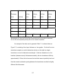
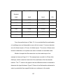
Table 3-1: Material Properties of Solids
Material
Speed of Sound
Density
Acoustic Impedance
m
s
kg
m3
kg Pa ⋅ s
m 2 ⋅ s = m
Copper
5010
8.93x10³
44.74x10⁶
Brass
4700
8.60x10³
40.42x10⁶
Speed of Sound
Density
Acoustic Impedance
m
s
kg
m3
kg Pa ⋅ s
m 2 ⋅ s = m
Water
1497
1.00x10³
1.50x10⁶
Methanol
1103
0.79x10³
0.87x10⁶
Glycerol
1904
1.26x10³
2.34x10⁶
Ethylene Glycol
1658
1.11x10³
1.81x10⁶
n-Pentane
1006
0.63x10³
0.63x10⁶
Table 3-2: Material Properties of Liquids
Material
32
Table 3-3: Material Properties of Vapors at room temperature
Speed of Sound
Density (at 1atm)
Acoustic Impedance
m
s
kg
m3
kg Pa ⋅ s
m 2 ⋅ s = m
Water Vapor
405
0.6
243
Methanol Vapor
335
.48 (est.)
160.8
Material
n-Pentane Vapor
Approximately Equal to Methanol (non-critical parameters)
B. Theoretical Basis of Film Thickness Estimates
1. General Overview
The structures to be probed acoustically using the ultrasound pulse-echo
system described in this thesis are fundamentally made up of three layers. The
first layer encountered by the ultrasonic pulse is the copper layer; this is followed
by the thin fluid layer formed by condensation and finally the air (or other vapor)
layer. The air layer is assumed to be semi-infinite, and the time scale examined
is limited to a short enough period to allow the copper layer to be modeled as
semi-infinite as well. Because of these assumptions, the situation can be
modeled as a finite fluid layer between semi-infinite copper and air layers.
The ultrasound pulse generated by the transducer is of finite duration,
consisting of approximately three cycles due to a very short excitation voltage
pulse; as a result, for fluid layers which are thicker than the spatial extent of the
33
pulse the behavior of the system can be modeled in the time domain as a single
pulse propagating through the layered model. In this case, a simple time domain
model using only transmission and reflection coefficients at the materiel
interfaces may be used. However, for layers less than approximately 1.5
wavelengths thick, there will be interaction between successive echoes in the
fluid layer. The effect of this interaction is most suitably observed in the
frequency domain.
Section 2, below, analyzes the system for the thin-layer case and Section
3 performs an analysis on the thick-layer case. The final section in this chapter
will discuss the effects of a fluid film which is not uniformly thick, and their
implications on ultrasonic measurement of such films.
2. Thin Layers: Frequency Domain Analysis
Although non-uniform fluid layers are too complex to treat analytically, the
case of the simple uniform fluid film is much more amenable to such a treatment.
The three layers of such a structure are defined in Figure 3-1:
34
Figure 3-1: Defining the Regions of a Simple Fluid Layer
The transducer is not perfectly coupled in the sense that there is an
acoustic impedance mismatch between the transducer and the copper block.
The effect of the mismatch is a longer pulse, but to simplify the situation for the
purposes of this discussion the transducer is assumed to be perfectly coupled
into the copper block. This assumption is invalid, but acceptable, since the
performance of the system does not strongly depend on the nature of the
ultrasound pulse, as will be shown in Chapter 4, Signal Processing.
35
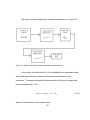
The system can be modeled from a systems standpoint as in Figure 3-2:
Figure 3-2: Model of thin-film (frequency domain) system behavior
In this model, the initial pulse P(ω,0) is multiplied by two attenuation terms
and a fluid layer reflection coefficient before being received back at the
transducer. The signal received at the transducer from this type of system can
thus be described by (3-18):
2
P (ω , x) = P (ω ,0) ⋅ e −2⋅α0 ⋅ω d ⋅ Rlayer
where d is the thickness of the copper block.
36
(3-18)
The complex, frequency-dependant reflection coefficient for a layer is
given in (3-19):
r1
1 − cos(k 2 ⋅ L) +
~ r3
R=
r1
1 + cos(k 2 ⋅ L) +
r3
r r
j 2 − 1 sin( k 2 ⋅ L)
r3 r2
r r
j 2 + 1 sin( k 2 ⋅ L)
r3 r2
(3-19)
Definition of Terms:
r1 = acoustic impedance of copper
r2 = acoustic impedance of fluid
r3 = acoustic impedance of air
k2 = wave number in fluid, i.e.
ω
c
or
2 ⋅π ⋅ f
c
where ω and f are frequency terms and c
is the sound speed in the fluid layer
L = thickness (in meters) of fluid layer
~
The expression for R , given in (3-19), may be separated into real and imaginary
parts:
r 2 r 2
r 2
2⋅r ⋅r 2⋅r
2
1
1 − cos θ + 2 − 1 sin 2 θ
12 2 − 1 sin θ cosθ
r3 r2
r2
~ r3
r3
R=
+ j
2
2
2
2
r2 r1
r1
2
2
1 + r1 cos 2 θ + r2 + r1 sin 2 θ
1
cos
θ
sin
θ
+
+
+
r3
r3 r2
r3 r2
r3
(3-20)
where
37
θ ≡ k2 ⋅ L =
2 ⋅π ⋅ f ⋅ L
c
(3-21)
While (3-20) gives the response of the entire layer, the echoes from the copperwater interface are much larger in magnitude than the echoes from the fluid-air
interface which have back-propagated through the fluid layer. Since the latter
echoes are the portion of the signal containing thickness data, it is desired to
extract them from the total echo signal. To do this, an equation for the echoes
from the copper-water interface is developed by simply using the equation for the
reflection coefficient from a simple boundary (3-22):
Rboundry =
r2 − r1
r2 + r1
(3-22)
Noting that (3-22) is entirely real, it is then subtracted from the real part of (3-20)
to yield the echo of interest (REOI) (3-23).
~
REOI
r 2
r 2 r 2
2
1
1 − cos θ + 2 − 1 sin 2 θ
r3
r3 r2
r2 − r1
−
=
+
2
2
+
r
r
r1
2
1
r
r
2
2
2
1
1 + cos θ + + sin θ
r3
r3 r2
2⋅r ⋅r 2⋅r
12 2 − 1 sin θ cosθ
r2
r3
j
2
2
1 + r1 cos 2 θ + r2 + r1 sin 2 θ
r3
r3 r2
(3-23)
38
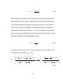
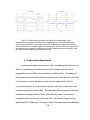
The magnitude of (3-23) is plotted in Figure 3-3, using values which correspond
to a 0.2mm thick water layer with the appropriate impedances for copper, water,
and air.
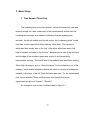
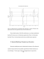
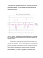
Figure 3-3: The Magnitude of the Frequency Response of a 0.2mm Water Layer.
Note the peaks at f0=1.85MHz, as well as 3 f0=5.55 MHz and 5 f0=9.25MHz.
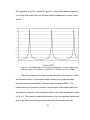
The pulse incident on the layer from the transducer is the result of exciting
the transducer with a ½ cycle square wave, resulting in a roughly Gaussian
spectrum spanning several MHz of spectral width centered at 5MHz. The
multiplication in the frequency domain of the spectrum of the incident pulse and
the frequency response of the transducer results in the received spectrum shown
in Fig. 3-4. The situation modeled here results in only one significant visible peak
due to very little spectral energy being emitted from the transducer at low
39
frequencies such as the f0 peak at1.85MHz and higher frequencies such as the
3f0 peak at 9.25MHz. With thicker layers, f0 – and thus the interval between
peaks – decreases resulting in multiple peaks occurring within the frequency
range which has significant spectral energy. Since this will cause more peaks to
be in the visible region (i.e. the region with sufficient spectral energy to be seen),
this will result in multiple peaks seen in the received signal. An example of such
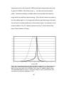
a case is shown in Fig. 3-5, which is the same as Fig. 3-4 with a thicker fluid
layer (0.5mm instead of 0.2mm).
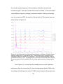
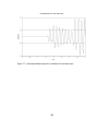
Figure 3-4: Normalized Analytically Predicted Received Signal for a 0.2mm water layer
with a 5MHz center frequency transducer excited by a 5MHz ½ cycle square wave.
Note only one major peak, at 3f0=5.55MHz. The f0 peak at 1.85MHz is barely visible.
The transmitted spectrum used (i.e. transducer output) is shown superimposed, also
normalized to a maximum amplitude of 1.00.
40
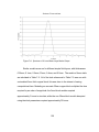
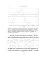
Figure 3-5: Normalized Analytically Predicted Received Signal for a 0.5mm water layer
with a 5MHz center frequency transducer excited by a 5MHz ½ cycle square wave.
Note obvious major peaks at 5f0=3.70MHz, 7f0=5.18MHz, and 9f0=6.66MHz. The f0 peak
at 0.74 MHz is not seen at all, and the 3f0=2.22MHz is barely visible.
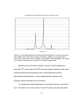
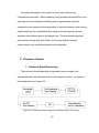
Spectra such as the ones in Figures 3-4 and 3-5 can be obtained by
taking the FFT of the output of the P/R unit in the system described in this thesis,
and these experimental results have been in good agreement with the
theoretically predicted spectra. Using a peak-detection algorithm, the f0
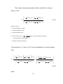
frequency can be extracted from such spectra.
To calculate the relationship between f0 and layer thickness, we note that
Fig. 3-3 (as well as, of course, Figures 3-4 and 3-5) show spectral peaks when
41
θ=
θ=
π
2
π
2
+ nπ using the definition of θ given above in (3-21). Solving (3-21) for
(i.e. f = f0) results in (3-24):
π
2
=
2π ⋅ f 0 L
c
(3-24)
which can easily be rearranged to give (3-25):
L=
c
4 ⋅ f0
(3-25)
(3-25) gives a simple relationship between f0 and the thickness of the fluid
layer, L. This allows the thickness to be easily calculated via Fourier analysis as
outlined above.
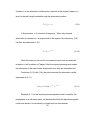
3. Thick Layers: Echo-Ranging
In the discussion in the previous section, the incident signal was assumed
to have sufficient length that interactions occurred between subsequent echoes
in the fluid layer. Clearly, if this is not the case than constructive and destructive
42
interference are not possible subsequent echoes will simply be seen as separate
pulses. Because of this, for fluids which are greater than approximately 1.5
wavelengths thick – since the incident pulse is only approximately three cycles
long – a different method must be used. This “thick layer” method is much
simpler that the analysis of thin layers, as it simply measures time differences in
the time domain.
If the ultrasound pulse is emitted with waveform p(t,0) it can be
represented as in (3-14):
p(t , x) =
+∞
∫ P(ω ,0) ⋅ e
j (ω ⋅t − kx )
⋅ e −α0 ⋅ω
2
⋅d
⋅ dω
(3-14)
−∞
As discussed above the only advantage of (3-14) over the much simpler
(3-3) is that (3-14) can account for attenuation; however, since the amplitude of
the received pulse is not important in the determination of film thickness, the
attenuation can be disregarded and (3-3) can be used instead:
x
p(t , x) = p(t ,0) ⋅ δ t −
c
(3-3)
After traversing the copper block, which is a distance b thick and has a sound
speed of cb, the pressure pulse will be time-shifted but otherwise unchanged:
43
b
p (t , b) = p (t ,0 ) ⋅ δ t −
cb
(3-26)
The portion of the pulse which is reflected back to the transducer without
entering the fluid layer is the product of the reflection coefficient Rc/f (indicating
the reflection coefficient for a pulse traveling from copper to fluid) and the pulse
in (3-26); after traversing the copper block back to the transducer, the received
pulse is:
2b
p (t , b) = p (t ,0 ) ⋅ δ t − ⋅ Rc / f
cb
(3-27)
In comparison, if no fluid layer is present it can be assumed that r2=0 since
air, and the fluid vapors used, have acoustic impedances several orders of
magnitude less than copper; in this case, the equation given for the reflection
coefficient of an interface given as (3-16) yields R = -1. The reflection coefficient
of no fluid – i.e. a copper/air interface – and the reflection coefficient of a semiinfinite layer of fluid would therefore be expected to be a factor of (-Rfluid) different
in amplitude. This will be shown to be a useful fact in Chapter 4.
The pulse which does enter the fluid layer will be the product of (3-26) and
the copper/fluid transmission coefficient, Tc/f :
44
b
p (t , b) = p (t ,0 ) ⋅ δ t − ⋅ Tc / f
cb
(3-28)
The pressure pulse described by (3-28) is time-shifted further by crossing
the fluid layer, and then reflects off of the fluid/air interface. It is then again timeshifted by propagating back through the fluid layer to the fluid/copper interface.
On its arrival at the fluid/copper interface, it can be represented by (3-29); in (329), Rf/a is the reflection coefficient at the fluid/air interface, cf is the speed of
sound in the fluid, and f is the thickness of the fluid layer:
b 2 f
⋅ Tc / f ⋅ R f / a
p(t , b, f ) = p(t ,0) ⋅ δ t − +
c
c
f
b
(3-29)
This pulse then is transmitted through the fluid/copper interface with
transmission coefficient Tf/c, and after propagating back through the copper block
arrives at the transducer as:
2b 2 f
p(t , b, f ) = p(t ,0) ⋅ δ t − +
cb c f
⋅ Tc / f ⋅ R f / a ⋅ T f / c
(3-30)
Since the first echo from the fluid layer was described by (3-27), the time
delay between (3-27) and the first echo from the fluid layer (3-30) can be easily
seen to be ∆t, defined as:
45
∆t =
2f
cf
(3-31)
The two signals described by (3-27) and (3-30) will have the same pulse
shape as long as all transmission and reflection coefficients are entirely real,
since the only difference between the two equations is a lower amplitude in (330) due to transmission/reflection coefficients (as well as due to attenuation,
which was neglected in this discussion) and a time-shift. Since both reflection
coefficients are negative, while both transmission coefficients are positive, the
two signals are the same polarity as well.
In other words, if an echo which appears the same as the previous echo –
except with lower amplitude – arrives at the transducer a time lapse of ∆t µs after
the previous echo this time lapse corresponds to the round trip travel time
through the fluid:
∆t =
2L
c
(3-32)
If subsequent echoes can be observed as discrete pulses, the time lapse
∆t between them is easily measured. Given ∆t, (3-32) solved for L yields a
simple equation to find L from ∆t:
46
L=
∆t ⋅ c
2
(3-33)
4. Films with Non-Uniform Thickness
In earlier sections of this chapter, it was assumed that all ultrasound
waves encountering interfaces were at a normal incidence. This is a valid
assumption for uniform fluid films, since the ultrasonic waves are traveling in a
vertical direction and all interfaces are horizontal. However, for nonuniform films
the surface of the film is not exactly horizontal, and thus the waves encounter the
interface at an oblique incidence.
Instead of carrying out an extensive analytical treatment of this case, it
was modeled using numerical modeling software which will be discussed in
Chapter 5. In general, it was found that slight nonuniformities did not significantly
impact the performance of the ultrasound system; however, larger
nonuniformities resulted in most of the ultrasonic energy being reflected away
from the transducer and thus a significantly degraded signal-to-noise ratio and
inability to measure the layer thickness. Full results of this modeling are
presented in Chapter 7.
47
Chapter 4: Signal Processing and Algorithms
A. Overview
The basic conceptual model for the ultrasonic fluid layer thickness
measurement system is shown below in Figure 4-1:
Figure 4-1: Basic Conceptual Model of Ultrasonic Fluid Layer Thickness
Measurement System.
After the raw RF data has been acquired from the pulser/receiver by the
digitizer, but before a thickness estimate can be made, a significant amount of
signal processing must be done for a successful measurement to occur. There is
some basic processing that is needed for all sets of data whether the thick-film or
thin-film algorithm is to be used; once this is done, there is a large amount of
additional processing specific to the thin-film algorithm if it is needed. This
48
chapter discusses all signal processing as well as the structure of the LabVIEW
control and measurement program.
1. LabVIEW Control Program Structure and Flow Chart
The LabVIEW control program is described in detail in Appendix B,
LabVIEW Program Technical Manual, but the general program structure and
signal processing algorithms are described here.
The overall control program consists of three main modules. These are
the main module, the communications module, and the baseline acquisition
module. The main module is what the user interacts with when acquiring data,
and it is also the program which contains the bulk of the signal processing and
interpretation software. The communications module has only one function: to
control and communicate with (including retrieval of raw data) all hardware in the
system. Since it performs no signal processing at all, and has no user
interaction, it will not be described further in this chapter. The baseline
acquisition module, as the name implies, acquires the baseline sample which will
be used to normalize all future data. This module performs a limited amount of
signal processing, and will be addressed briefly.
The general flow chart of the LabVIEW program is shown in Figure 4-2.
49
Figure 4-2: LabVIEW control program overview flow chart
As can be seen from Figure 4-2, there is a limited amount of data
processing common to both time and frequency domain methods; however, the
time domain method requires very little additional data processing beyond this
point while the frequency-domain method requires a significant amount.
50
2. Signal Processing Common to both Thin and Thick Films
The RF signal received by the digitizer from the transducer via the
pulser/receiver consists of the desired signal – that which contains information
about layer thickness – in addition to a much larger amount of “noise”. In this
case, “noise” does not refer to the traditional Gaussian “white noise”, but rather to
artifacts in the form of unwanted portions of the signal which contain no useful
data and which obscure the useful data that is present. These artifacts include
the result of such phenomena as grain scattering within the copper block and the
copper/fluid interface echo. The latter would appear at first glance to be part of
the useful signal, but is not in fact useful since the distance from the transducer
to the far side of the copper block is not the distance being monitored and this
echo carries no information about the fluid layer whatsoever. This copper/fluid
interface echo is in fact harmful since it can bury useful data due to its much
larger amplitude.
The relative magnitudes of the desired (data-containing) signal and the
artifact signal result in an extremely low effective SNR. This SNR varies with the
fluid and with the thickness of the copper block, but averages roughly 0.1
(= -20dB). However, since the artifact components of the received signal can be
mostly removed, a significant SNR improvement can be achieved. The reason
for this nearly complete removal is that both the grain scattering from within the
copper block and the copper/fluid echo are very repeatable.
51
The copper/fluid interface echoes are, in fact, the exact same for each
pulse with a given fluid and a given transducer location. If the fluid layer can be
made thick enough such that the first fluid/vapor interface echo does not arrive at
the transducer until well after the first copper/fluid echo has been received, this
artifact signal can be recorded. However, often the echo from the bare copper
block (no fluid layer) is easily recorded but creating a thick fluid layer to record for
normalization is impractical; in these situations, the copper/fluid echo can be
calculated from the copper/air echo and the ratio of the reflection coefficients of
copper/air and copper/fluid. The system is set up to allow the acquisition of the
baseline signal with a bare copper block, after which it scales the portion of the
signal which is the copper/air echo to correct it so that it can be used to cancel
out the copper/fluid echo. The rest of the signal, meaning the signal segment
which comes before the copper/air echo is received, is left unscaled as it is a
result of scattering within the copper block and is not affected by the presence of
the fluid. Theoretically, this method should be perfect; however, in practice, it is
not as effective as an actual measurement of a very thick fluid layer since the
artifact cancellation is not as complete. As a result, an actual “baseline”
measurement of a very thick fluid layer is the desired method with the calculated
method acting as a marginally acceptable backup if creating a very thick film is
impractical.
Since the raw RF signal from thin fluid layers is simply a sum of the artifact
signal and the data-containing signal, only the useful portion of the signal
52
remains once the previously recorded or calculated artifact signal is subtracted.
By doing this point-by-point subtraction, which is computationally very simple and
thus does not add much time to the data processing, the SNR is improved
greatly. An example of pre-subtraction and post-subtraction signals is shown in
Figure 4-3 using simulation data for a thick film.
Figure 4-3: Extraction of the Desired Portion of the Signal. “Raw”, upper left: the
unprocessed signal, “Baseline”, upper right: the previously stored “baseline” signal
obtained with a bare copper block and uncorrected for reflection coefficient, and
53
“Normalized”, bottom: the processed signal. The scales of all three frames are the
same.
A problem which has been solved in the current system is the importance
of trigger synchronization. If the sample clock of the digitizer is not synchronized
with the trigger source for the pulser/receiver, the resulting time offset of up to
plus or minus one half of a digitizer sampling period will cause the normalization
to be inaccurate. This does not significantly affect the time-domain method,
since it is simply looking for large peaks in the time domain, but it can cause
significant distortions in the Fourier transformed data. The current system uses a
built-in synchronous trigger output in the digitizer to trigger the pulser/receiver;
any future system will need to incorporate such a feature as well.
The signal processing up to this point, primarily consisting of the removal
of the artifact caused by the copper/fluid echo, is carried out for every sample
acquired regardless of whether the time domain or frequency domain method of
measurement is to be used; the processing specific to each method is described
in the next sections.
B. Time Domain
1. Detection of ∆t and Calculation of Layer Thickness
Conceptually, the time-domain algorithm is fairly simple. The first fluid/vapor
interface echo to return to the transducer will be result in a negative voltage pulse
54
received at the digitizer, and will in fact be the most negative voltage seen for the
entire sample period once the artifacts discussed above have been subtracted.
The exact time that the first copper/fluid interface echo returns to the transducer
can be easily seen from the “baseline” dataset – by simply finding the most
negative point, and noting the timestamp – and the exact time that the first
fluid/vapor interface echo returns to the transducer can by found by a similar
method using the processed (i.e. post baseline subtraction) data set. Simply
determining the difference between these two times gives the round-trip travel
time within the fluid layer, which by (4-1) easily yields the layer thickness.
L=
∆t ⋅ c
2
(4-1)
One problem encountered in the calculation of the time-domain thickness
algorithm is that the peak of the first fluid/air echo will sometimes not be the most
negative point in the post-normalization dataset; this can be cause by noise or
slight changes in transducer position resulting in an inaccurate “baseline”
dataset. In either case, a system which simply looks for the most negative point
in the dataset will not always successfully detect the actual thickness. In order to
minimize this problem, a windowing algorithm was set up. Instead of looking for
the most negative point in the entire dataset, the algorithm looks only for the
most negative point within a set time before and after the previous value. The
width of the window can be changed by the user while measurements are in
55
progress, and the width below the previous value and above the previous value
can be changed independently. This allows the user to set the window to allow
for the tracking of drops falling off, and thus a suddenly thinner layer, but not
allow for sudden layer growth. The second-largest peak in the normalized signal,
and thus the one most likely to momentarily exceed the magnitude of the desired
peak, is generally either the second fluid-air echo or the second copper-fluid
echo. Since both of these are after the peak of interest, setting a window which
allows sudden decreases but not sudden increases will track anticipated events
such as drop departure but significantly reduce the effects of noise.
2. Limitations of Time-Domain Method
This algorithm works quite well as long as the artifact cancellation by
baseline subtraction performs as expected. If the “baseline” is not accurate, for
example if the transducer position has shifted slightly since the “baseline” dataset
was acquired, significant interference will be present in the processed dataset
and this method is less reliable. However, a fairly significant change in the
baseline is necessary before this occurs.
There are three main limitations to this method. The first is that the digitizer
must acquire data for a sufficiently long time to capture the first fluid/vapor
interface echo returning to the transducer. This only creates a problem for very
thick (>5cm for the current system) layers, and if necessary can very easily be
changed by simply acquiring data for a longer period. However, the sample
56
period to be used must be determined before the experiment commences due to
the need to acquire a “baseline” of suitable length before actual experimentation
starts. This means that if an unexpectedly thick layer were to be encountered
during experimentation, it may not be able to be monitored if not planned for
ahead of time.
The second main limitation is that the resolution is limited by the sampling
rate of the digitizer. Since the algorithm simply records the time stamp of the
point with the most negative amplitude, the time resolution is determined by the
sampling frequency of the digitizer. This means that for the 20Msamples/s
digitizer used, the time resolution is 50ns. From Equation (3), this corresponds to
35 microns (in the case of water). This means that the output of this algorithm
will always be a multiple of 35 microns, creating a resolution of 35 microns for
this method. If a resolution finer than this is required, it can be easily obtained by
using an digitizer with a faster sampling rate. For example, a 100Msample/s
digitizer would correspond to a 7 micron resolution. The 20Msample/s digitizer
currently in use was selected because it was the fastest digitizer with a PCMCIA
interface available; a faster digitizer would result in the need for an digitizer
external to the laptop used and thus an additional piece of equipment for a
theoretically easily portable system.
The third limitation is that this method is not suitable for very thin films (<500
microns). At these thicknesses, the individual echoes are not easily discernable
and the frequency-domain algorithm is more appropriate.
57
One major advantage to this method is that it uses relatively few
computational resources. When measuring using multiple transducers this is not
important since the multiplexer switching time is approximately twice the
computation time required for both algorithms to execute; however, when using a
single transducer the computational time required for the frequency-domain
algorithm is the limiting factor in the sample rate. The time-domain algorithm
executes fast enough that other factors, such as the digitizer-software
communication, are rate-limiting rather than the algorithm.
C. Frequency Domain
1. Additional Signal Processing
The frequency-domain algorithm is significantly more complex both
conceptually and computationally than the time-domain method. It is shown in
block-diagram form in Figure 4-4.
Figure 4-4: Frequency-Domain Algorithm Additional Signal Processing
58
After the signal is preprocessed (i.e. the “baseline” is subtracted out), the
dataset appears to be a series of “ringing” signals. Each time the fluid layer is
excited either by the original short pulse from the transducer or by an echo of that
pulse, the reflected signal from the layer is a decaying sine wave with
fundamental frequency f0. This fundamental frequency can be used in (4-2) to
find the fluid layer thickness. Isolating this frequency entirely automatically
without human input can be quite challenging, however.
The first step in the process is to multiply the signal with a “flat-top”
enveloping function. This has the effect of tapering the ends of the data array
without affecting the center portion significantly. This filter is done by a point-bypoint multiplication with the center half of the signal being multiplied by unity
while both the beginning and end quarters are multiplied by coefficients which
taper from unity at the center of the segments to zero at the ends. This filter is
used to cut down on noise in the next step of processing due to sudden drops at
the ends of the data segment. Because the rolloffs of the filter are not variable,
the effect of the filter is changed by zero-padding the signal slightly at both ends
before passing through the flat-top enveloping function. The user can select the
amount of zero-padding; increased zero-padding results in a more accurate
signal due to less of the actual signal being lost in the beginning and end portions
of the sequence which are reduced by the envelope function. However, less
zero-padding results in less abrupt transitions at the beginning and end of the
time-domain signal which significantly reduces the noise seen after the FFT.
59
Approximately 50-100 zeroes are usually added to each end of the time-domain
signal prior to the envelope function; with a signal of interest typically
approximately 300 points long this results in a fairly low-noise FFT without too
much signal loss.
As seen in Figure 4-4, the next step is to again zero-pad the signal. The
signal under analysis may only be several hundred data points long; it is
symmetrically padded at both ends with zeroes to create a sequence which is a
power of 2 long to allow for a computationally efficient FFT. An 8192- or 4096point total sequence (original data plus pre-enveloping and pre-FFT zeropadding) is usually used, but the exact value is user-selectable and can be
changed for each measurement run. A higher value allows for higher resolution,
but a lower value allows for lower computation time if faster sampling is desired.
The next step is a fast Fourier transform, resulting in a frequency
spectrum. This frequency spectrum is then used to calculate the layer thickness,
as described in the next section.
2. Detection of fo and Calculation of Layer Thickness
The spectrum resulting from the processing above is analyzed with a
peak-detection algorithm to identify the spectral peaks; a flow chart is shown in
Figure 4-5.
60
Figure 4-5: Peak-Detection Algorithm Flow Chart
This peak detection algorithm begins by identifying the highest peak in the
spectrum. If there is no peak with amplitude greater than a set minimum, the
data is deemed invalid and f0 is reported as “NaN” (“Not a Number”); this is done
to avoid treating noise as valid data if no actual spectral peak is present as in the
61
case of no fluid layer at all. Once the highest peak has been detected, the
values of the array containing the FFT data are set to zero for a preset frequency
interval surrounding the location of the highest peak. This interval is set based
on previous layer measurements and is one of the largest challenges in this
algorithm; if it is too narrow, a broad peak may be read as two peaks if while if it
is too broad only every other peak will be detected. In either of these cases,
erroneous data will be reported.
The algorithm then detects all other peaks in the spectrum which are
greater than a set percentage of the height of the highest peak by finding the
highest remaining peak, setting the surrounding portion of the array to zero, and
repeating until the highest remaining peak is less than the set percentage of the
original highest amplitude peak.
Spectral peaks occur at odd multiples of f0, i.e. f0, 3f0, 5f0, and so forth.
Since for thicker fluid films the f0 – and sometimes 3f0 and 5f0 – peaks are not
visible, the interval between each pair of adjacent spectral peaks is calculated
and all intervals in a given spectrum are averaged. The average interval is
divided by 2 to yield f0, which is then used in (4-2) to calculate the layer
thickness.
L=
c
4 ⋅ f0
62
(4-2)
If only one identifiable peak is detected, as happens with very thin fluid
layers, the peak-detection algorithm cannot perform in this manner as no
intervals exist in the spectrum; in this case, the frequency of the sole peak is
deemed fo.
3. Limitations of Frequency-Domain Method
The frequency-domain method works well for films which exceed a
minimum detectable thickness of approximately 50 microns but are thin enough
that the echoes from the fluid/vapor interface create a signal with enough of a
resonant character to analyze. At fluid layers thicker than approximately 1mm
(1000 µm) in water, the fluid/vapor interface echoes become too discrete to
analyze using this method. The critical thickness in other fluids scales linearly
with the speed of sound, with slower sound speeds resulting in thinner critical
thicknesses. Because the time domain method works at layers as thin as 500
microns, this creates a sufficiently large overlap zone in which both work, from
thicknesses of 500 to 1000 µm. The current system switches over at 750 µm;
below this level the frequency domain algorithm is used while at above this level
the time-domain system is used. It is desired to use the frequency-domain
method for as long as possible, since its resolution is on the order of five µm
compared to the time domain method’s 35 µm resolution, but it becomes
63
increasingly unreliable as the layer grows thicker so 750 µm was chosen as an
optimal changeover point.
As with the time-domain algorithm, the frequency-domain method has
several drawbacks. The first is that if the fluid layer is too thin, not enough of an
echo is generated to be detectable. In tests with water, a layer as thin as 50 µm
has been monitored; however, it is unknown at present how thin a layer is
actually detectable as no water layer thinner than 50 µm was stable enough to be
measured. It is anticipated that this method will work at thinner layers than are
stable with many fluids, and in any case down to at least 50 µm as seen in the
lab, so this limitation is not expected to be a factor with the current research.
For thicker layers, specifically layers thicker than approximately a
millimeter in water, f0 becomes very low and is increasingly difficult to detect.
Because f0 becomes low, the adjacent peaks in the frequency spectrum become
more closely packed together and less distinct. Since f0 is calculated based on
the spacing of adjacent peaks, if the peaks are indistinct f0 can not be calculated
so this algorithm fails. In lab experiments, fluid layers as thick as 2mm in water
have been measured with this method; however, at thicknesses over 1mm this
method is increasingly unreliable. In the few cases that the frequency-domain
algorithm has successfully measured films as thick as 2mm, several attempts
were required to produce a valid thickness estimate.
Finally, for fluid layers with variable thickness, for example if the peak of a
wave is visible over half of the beam and the trough the other half, the spectrum
64
will have peaks from both thicknesses. This is usually not a problem with a 6mm
transducer and a copper block thin enough that the fluid film is located in the
near field since most fluid phenomena which could cause this are no smaller than
the beamwidth. However, in trials with thicker copper and brass blocks where
beam spreading phenomena result in an effective beamwidth of 10-15mm this is
a commonly encountered problem which makes automated peak-detection
unreliable. This is also a problem with dropwise condensation before a layer
forms, since bare copper over part of the beamwidth and a thin layer over
another part can cause the same effect. For a continuously varying thickness, as
in the case of a slanted film, numerical models have shown that a 45% difference
from the center of the beam to the edge can cause sufficient perturbation to the
resonance to make it impossible to generate a thickness estimate even under
ideal conditions. Under actual experimental conditions, a considerably smaller
degree of difference will make measurements difficult.
D. Additional Topics
1. Transducer Excitation
The pulser-receiver currently used in this system excites the transducer
with a single half-square-wave of selectable duration. The original pulserreceiver used a more conventional delta-function excitation. Theoretically, the
new P/R will couple more energy into the transducer since it is an excitation near
65
the natural resonant frequency of the transducer rather than an extremely
broadband signal. When the tuneable P/R became available, it was evaluated at
several different frequency settings to determine whether it had any advantage
over the conventional P/R; the results of this test with a 0.75mm water layer are
shown below as Figure 4-3.
Figure 4-6: An Evaluation of an Untuned Pulser-Receiver vs Different Tuneable PulserReceiver Settings for a 0.75mm Water Film. The horizontal axis is a frequency axis,
calibrated in MHz; the vertical axis is amplitude. Each successive dataset is offset on
the amplitude axis by 1,000. The bottom trace is from the old (untuned) pulser-receiver;
the seven above it are the tuneable P/R unit with the highest frequency settings at the
top.
From Figure 4-6, it is clear that the tuneable pulser-receiver had better
performance than the untuned unit for very low frequencies (below 2 MHz) with
any setting; with settings such as the 3.5 MHz center frequency (the purple trace
66
which is offset by 4,000) the tuneable pulser-receiver had better performance
than the untuned unit for all frequencies below 5MHz.
2. Signal Averaging
When acquiring the baseline signal, acquisition time is not particularly
important but noise minimization is very important; if the baseline signal is noisy
then all measurements made using that baseline for normalization will be noisy
as well. Because of this, the baseline acquisition is done by averaging together
1,000 separate acquisitions for each transducer. This takes several seconds, so
clearly is not practical when acquiring thickness data; however, with particularly
noisy data which is the result of a stationary or slow-moving fluid layer it is
possible to average together a small number of acquisitions (usually two to five)
to reduce noise. The more datasets used for averaging, the less noisy the data
will be; however, the longer acquisition time means a lower sampling rate. In
addition, if the conditions in the fluid film are rapidly changing signal averaging
can be counterproductive. This can occur when, for example, five signals are
acquired for averaging over the course of perhaps 50 ms; if the layer thickness
over the transducer is changing while this occurs, the five samples will be
different which will act to create more noise. However, in the case of low SNR
due to high noise when the fluid film is not rapidly changing, signal averaging can
help significantly. Signal averaging is user-selectable, and can be changed
during the experiment.
67
Chapter 5: Acoustic Numerical Modeling
A. Introduction
1. Goals for Modeling Experiments
Due to the complexity of the ultrasonic measurements undertaken in the
course of this research, analytical modeling beyond the most basic conceptual
models discussed in Chapter 3 is not a realistic option. However, some method
of predicting the experimental behavior – and thus helping to verify that it was
indeed what was expected rather than some unforeseen effect – was deemed
important. Numerical finite time difference modeling was the clear choice as an
alternative to analytical methods, and this was in fact the modeling method used.
The goals of these numerical modeling experiments were to predict the acoustic
behavior of the actual physical experiment and then, once the physical
experimental setup was assembled, to verify that the results of the physical setup
could be reproduced using modeling thus showing that the experiment was
behaving in a predictable manner.
Once the initial simple numerical models had been shown to correlate with
the results of the initial simple physical experiments, namely static noncondensing films, numerical modeling was used to predict the behavior of hardto-create physical states. For example, numerical modeling was used to
determine the sensitivity of the frequency-domain thin-film measurement method
68
to local thickness variation in the fluid layer. Acoustic modeling of a fluid layer
with well-characterized variations in thickness is an easy task; however, actually
carrying that experiment out in a physical model would be much more inexact.
Another example of the usefulness of modeling is determining the response of
the measurement system to droplet formation in the fluid layer. Numerical
modeling of the received signal from a droplet of known dimensions is again
relatively straightforward, while creating a physical drop of known and repeatable
dimension and location is nearly impossible. The closest approach to this in the
physical model would be to create actual droplets during condensation, but
because of the gravity field they would be a different shape and size than the
droplets expected in reduced gravity as well as being much less well
characterized than those in the numerical models.
In sum, the goals of numerical modeling were first to verify that the
physical experimental setup was functioning correctly and second to predict the
outcome of measurements in conditions which would be difficult to create in the
lab, but are expected to be seen in low-gravity operation.
2. Acoustic Modeling Software – Wave2000
The software used for acoustic numerical modeling was “Wave2000”,
created by CyberLogic Inc. Wave2000 is a two-dimensional ultrasonic modeling
software package written primarily for the non-destructive testing market, but it is
well suited for this project as well. A two-dimensional cross-section is defined,
69
and the algorithm used by the software assumes that the two-dimensional crosssection in the plane of the screen extends into and out of the screen infinitely far
with a constant cross-section of the object as defined on the screen. This results
in a slightly unrealistic model in a number of small ways; for example, the
transducer is modeled as being an infinitely long (in the direction normal to the
screen) rectangle instead of a circle. However, the results from Wave2000 agree
fairly well with actual experimental results so it is concluded that the effect of
using a 2-D model rather than a more realistic 3-D model are relatively
insignificant.
B. Modeling Theory used in Wave2000
1. Equation Used
Wave2000 represents the modeled objects as a series of grid elements,
and it solves the acoustic wave equation for each grid element for each time
step. The equation used is given below as (5-1). The equation and the
explanation of terms are from the User’s Manual to Wave2000.
70
∂2w
∂
∂ 1 ∂
= µ + ε del 2 w + λ + µ + φ + ε grad (del • w )
2
∂t
∂t 3 ∂t
∂t
ρ ⋅
kg
Where ρ = material density 3 ; λ = first Lame constant
m
N
Lame constant 2 ; ε = shear viscosity
m
(5-1)
N
m 2 ; µ = second
N ⋅s
m 2 ; φ = bulk viscosity
N ⋅s
m 2 ;
“grad” denotes the gradient operator; “del” denotes the divergence operator; •
denotes the vector “dot” product; ∂ denotes the partial difference operator; t =
time [s]; w is a two-dimensional column vector whose components are the x and
y components of displacement of the medium at location (x,y), that is,
w = [Wx( x, y, t ),Wy ( x, y, t )] where T indicates matrix transpose.
T
2. Explanation of Modeling Parameters
In addition to the geometry of the objects being modeled, there are several
parameters that control the performance of the Wave2000 software package and
which must be set appropriately. These parameters fall into the three major
categories of temporal, spatial, and material. The temporal parameters control
the size of the ∆t used between steps of the simulation, the spatial parameters
71
control the size of the grid used, and the material parameters determine the
materials being simulated.
a. Temporal Parameters
Based on the grid size as defined by the spatial parameters and the
velocity of sound in the materials being simulated, Wave2000 internally
calculates a suitable ∆t. This internally calculated value can be modified by the
user by setting the “time step” parameter; the actual time step used is the
internally calculated value, multiplied by the value entered by the user as the
“time step”. For example, with an internally calculated value of 0.1µs per step
and a user-entered value of 0.5 the actual time step used by the simulation would
be 0.05µs. For most modeling runs for this project, the user-entered time step
was set to 0.5 since at the default internally calculated time step (i.e. userentered time of 1.0) the simulation exhibited slightly unrealistic behavior.
Superficially the output looked correct, but after signal processing was performed
the resulting data was different enough from the experimental data to be
unusable. With a user-set factor of 0.5, the processed data nearly exactly
matches the experimental data.
The other two temporal parameters do not directly affect the simulation
processing itself. The first, simulation duration, simply determines the duration of
time for which the simulation is run. Simulation durations of approximately 510µs were common during this project depending on the thickness of the
modeled copper block; these durations were chosen to allow sufficient time for
72
the first echo from the fluid layer to return to the transducer while being short
enough to minimize computation time. The second parameter, display
frequency, controls how often the computer display was updated during the
execution of a simulation run. The default setting is 1, i.e. the display is updated
after every time step, but updating the display is a computationally intensive
process; it is unnecessary to monitor the progress that closely, and the decrease
in computation time by reducing the display frequency was significant. A display
frequency of 100 was usually used, meaning that after every 100 steps the
display would be updated. This value was chosen since it was infrequently
enough that it would not significantly slow computation time, yet it was often
enough to be able to see the progress of the simulation. In a few cases, the
images displayed were also saved as images to a file resulting in a “movie” of the
simulation; one “frame” every 100 steps was an appropriate rate for this.
b. Spatial Parameters
The first spatial parameters which must be set are those that control the
fundamental geometry of the model; these are the model size and the model
resolution in pixels per millimeter. Both of these are defined when the geometry
of the model is initially created, and cannot be modified subsequently. The
model size must be set large enough to contain all reflecting structures of
interest, and large enough that echoes off of the borders of the modeled area do
not reflect back and affect the simulation; however, the larger the modeled area
is, the more computer memory is required and the longer model execution takes.
73
The models used for this project typically took approximately three to eight hours
to execute on an 800-MHz AMD Athlon computer with 512MB of RAM, and many
were as large as could be accommodated without adding more RAM. The
largest models modeled were 32mmx30mm, taking approximately 30 hours to
simulate; more commonly used models were 12mmx20mm, requiring six to eight
hours. Some models testing only very specific ideas were smaller still, about
6mmx10mm, requiring only about an hour to simulate. Almost all models were
defined in 100pixel/mm resolution. The resolution, in pixels/mm, does not control
the grid size for the computation of the simulation; instead, it controls the feature
size of objects which can be included in the simulation. The 100 pixels/mm value
was selected to allow for very shallow slopes when investigating non-uniform
films.
Boundary conditions on all edges were set to “air”; meaning that at each
boundary of the model the software simulated what would happen if anything
outside the modeled area was simply air. It was desired to set the boundary
conditions such that the layers would be modeled as indefinitely wide (i.e.
echoless absorbing boundary conditions) but this was not possible due to
constraints of the software. This echoless absorbing boundary condition was
advertised to be an option for an update to Wave2000, “Wave2000 Pro”, but it
was decided not to invest in this software in favor of waiting for the next
generation software. The next generation software, “Wave2500”, is said to
model in “2.5 dimensions”. This means that it can model 3-D simulations
74
provided that they are axisymmetric, creating a cylinder by sweeping one plane
about a central axis at one edge of the replicated plane. As of the time this
writing (Spring, 2002), Wave2500 has been delayed multiple times and has still
not been released. A third generation of software, “Wave3000”, which would
model true three-dimensional models, will be the next step beyong Wave2500
but also has not yet been released.
Once the geometry has been defined, and the simulation is ready to run,
there are two run-time spatial parameters which must be set along with the runtime temporal parameters. These are the resolving wavelength and the
“points/cycle” parameter. The resolving wavelength, as the name implies, tells
Wave2000 the value of the smallest wavelength of interest; this is then used
along with the fastest speed of sound in any material in the model to calculate
the internally-generated time step. Unlike the time step, however, the program
does not internally generate a spatial step for grid spacing. The grid spacing is
directly determined by the user, using the “points/cycle” parameter. The grid
spacing used by the program is the resolving wavelength divided by the
“points/cycle” value. This means that theoretically a “points/cycle” of 2.0 should
satisfy the Nyquist criterion, but in practice a value of at least 4.0 is needed for
acceptable performance.
75
c. Material Parameters
When defining the initial model, the user selects a “gray level” (color) for
each different “material” in the model. Once the model is fully defined
geometrically, material properties are associated with each “gray level”. When
initially defining the geometry for a copper block with a fluid layer, three
rectangles are defined. One is made the correct thickness for the copper block,
and assigned “gray level 0”. The center rectangle is set to the thickness of the
fluid layer, and assigned “gray level 100”. The final rectangle is created on the
opposite side of the fluid layer from the copper block, and is assigned “gray level
255”. Gray level 255 is a reserved color which automatically indicates “void”, or
acoustically impenetrable vacuum. The other two gray levels are defined once
the geometry is complete to be copper for gray level 0 and water (or other fluid)
for gray level 100.
For each gray level used in the model except gray level 255, the user can
either select material properties from a library included in the Wave2000 software
package or input custom parameters. For all modeling done in the course of this
research, only library entries were used; specifically, those for copper, water,
methanol, and brass were used during the course of this research.
76
C. Model Setup
1. Time Domain (Thick Film)
The modeling done for the time-domain, uniform-thickness film, case was
relatively simple, as it was a case easy to test experimentally and as such the
modeling served simply as a means of verification that the modeling was
accurate. As with all models used for this project, the “condensing block” model
used was a solid copper block 20mm wide by 10mm thick. The transducer,
which was 6mm across, was on the “top” of the block while there was a fluid
layer of variable thickness on the “bottom”. Between the far side of the fluid layer
and the edge of the simulation space was a layer of void (acoustically
impenetrable vacuum). The overall size of the modeled area was 20mm wide by
20mm high, allowing for up to a 10mm fluid layer. For the initialization run of the
software, which created a baseline dataset with which to process all subsequent
datasets, a fluid layer of the full 10mm thickness was used. For the experimental
runs, layers between 0.5mm and 9mm were used (results from these
experiments are given in Chapter 7, “Results”).
An example of such a setup is shown below in Figure 5-1.
77
Figure 5-1. An image of a typical time-domain simulation geometry. The upper
black block is the copper condensing block, and the middle gray block is the fluid layer.
The bottom white block is “void”, which approximates air. The transducer is not visible in
this view, but is 6mm wide and is centered on the top of the “copper” block. The block
itself is 20mm wide by 10mm high, with a 4mm deep water layer and a 6mm “void” layer
to fill the 20mmx20mm simulation field.
The transducer was set to pulse-echo mode, with an excitation pulse of a
“sine Gaussian pulse” waveform, meaning that the pulse was a sine wave with
Gaussian envelope. This pulse was used for all modeling experiments, as it was
desired to model them all with the same transducer and excitation just as the
actual physical experiments used the same transducer and excitation. The sine
Gaussian pulse was chosen to be a signal with moderate bandwidth and a center
78
frequency (sine wave frequency) of 5MHz, which we believed to fairly closely
model the actual physical transducer characteristics. The specific excitation
wave is shown in Figure 5-2, below.
Figure 5-2. The excitation signal sent by the transducer in the Wave2000 model.
This is a “sine Gaussian pulse”, with amplitude enveloped by a Gaussian curve. The
parameters are set as shown, resulting in the largest amplitude being negative. The
actual physical transducer is excited by a negative-going square wave, but the
characteristics of the transducer result in a signal similar to that shown to be actually
injected into the copper block.
The run-time spatial and temporal parameters discussed above were set
as shown in Figure 5-3. These parameters were used for all models, not only
time-domain runs, as they were found to be the set which produced an accurate
simulation while using sufficiently little memory to be practical. Settings which
used less memory and computation time, for example a time step scale of 1.0,
produced anomalous results which did not match physically observed results.
79
Settings which would theoretically be more precise, such as setting the resolving
wavelength to 0.01mm, would require much more RAM than was available and
so were impractical. The settings shown below produced data which matched
physical data so far as was measurable while requiring only as much RAM as
was available; however, simulation time was in excess of eight hours for a single
run.
Figure 5-3. Run-time parameters used for Time-Domain models. These
parameters were used for all models, not only time-domain runs, as they were found to
be the set which produced an accurate simulation while using little enough memory to be
practical.
80
2. Frequency Domain (Thin Film)
The only difference between models designed for time-domain (thick film)
use and frequency-domain (thin film) use is simply the fluid film thickness. While
numerical modeling experiments to test the time-domain algorithm use 0.5mm9mm thick films, frequency-domain tests used 0.05mm (50 micron) – 1mm thick
films. Aside from this geometric change, all other settings were kept exactly the
same. As can be seen from the overlapping thickness ranges, films from 0.5mm
to 1.0mm thick could be, and in fact were, used to test both thin and thick film
algorithms since they modeled the transition region where both algorithms work
acceptably. An example of a thin-film geometry is shown in Figure 5-4.
81
Figure 5-4. An image of a typical frequency-domain simulation geometry. The
upper black block is the copper condensing block, and the very thin middle gray block is
the fluid layer. The bottom white block is “void”, which approximates air. The transducer
is not visible in this view, but is 6mm wide and is centered on the top of the “copper”
block. The block itself is 20mm wide by 10mm high, with a 0.25mm deep water layer
and a 9.75mm “void” layer to fill the 20mmx20mm simulation field.
3. Non-Uniform-Thickness Film
While the utility of the uniform-thickness film models was mostly in
verifying that the physical model was performing as expected, and even more so
to verify that the modeling was accurately representing physical reality, the nonuniform-thickness film models were intended more to explore phenomena which
was not easily created in a physical experiment. An example of this was the
82
exploration of wedge-shaped films, to determine how much nonuniformity can be
tolerated by the frequency-domain and time-domain algorithms. This was done
by creating a geometry with a slanted bottom edge to the fluid film, at an angle
and thickness calculated to produce a set variance in thickness across the
beamwidth. Figure 5-5 is a fairly extreme example, showing a 50% difference
between the left and right edges of the beam.
Figure 5-5. An image of a non-uniform film geometry. In this model, the
thickness of the fluid film varies from 225 microns on the left edge of the nominal
beamwidth to 375 microns on the right edge of the nominal beamwidth; this creates a
difference of 150 microns which is 50% of the 300 micron center thickness. The angle
used for the bottom surface of the water to achieve this is 1.43°, with a water layer
thickness on the extreme left edge of the 20mm model width of 0.05mm.
83
Another example was the simulation of films with droplets; droplets of
varying radial sizes, depths, and horizontal offsets from the transducer were
measured. Most of these droplets were modeled as semi-ellipsoids in the 2-D
plane of the screen, resulting in the numerical model of semi-cylinders since the
equations used in Wave2000 model a 3-D object with a constant cross section as
shown on the screen. However, some models using a series of small drops to
simulate the first phase of condensation before a film forms were modeled as a
series of semi-circles in the plane of the screen (resulting in the numerical model
of cylinders with semi-circular cross section). Two examples of these models,
one an offset single drop and the other a series of small drops, are shown as
Figure 5-6.
Figure 5-6. Two droplet models. On the left, a 5mm thick block is shown with
multiple 0.25mm radius droplets on its otherwise bare surface; the droplets are spaced
1mm center-to-center. On the right, a droplet consisting of a semi-ellipse with 2.0mm
horizontal diameter and 0.5mm vertical radius with a 0.2mm layer on the rest of the
block.
84
Aside from the geometry, all other parameters used in the non-uniformfilm models were exactly the same as in all of the other uniform-film models.
85
Chapter 6: Experimental Work
A. Experimental System
1. Overall System Description
The system developed by this project to carry out the ultrasonic
measurement of thin fluid film layers is contained in four physical parts, shown in
block diagram form below in Fig. 6-1.
Figure 6-1: A block diagram of the ultrasonic thickness measurement system.
The large box in the lower right is a Dell laptop, which contains a PCMCIA
digitizer in one of its expansion slots. The system is controlled by LabVIEW
software running on this laptop, and the PCMCIA digitizer is used to acquire the
86
ultrasonic data. The second major element to the system is a Panametrics
model 5077PR Pulser/Receiver unit. This unit generates the excitation pulses to
be sent to the transducers, and receives their detected echo signal which is
amplified and sent to the laptop/digitizer as the so-called RF signal. The
multiplexer is an Agilent 34970A multi-function device chassis with an Agilent
34903A general purpose switching card. This device is used to allow the single
P/R unit to be used with eight different transducers. The transducers
themselves, mounted on the copper block with their cabling attached, are the
final element in the system.
In operation, the LabVIEW software running on the laptop initiates a data
acquisition cycle by first setting the multiplexer to the correct channel via an RS232 serial communications bus and then sending a software trigger to the
digitizer. The digitizer has the capability to send a synchronous external trigger
pulse when it receives a software trigger, and so begins acquisition at the same
time it sends the external trigger pulse. This pulse is used to trigger the P/R unit
to generate a pulse to send to a transducer, via the multiplexer. The echoes
received by the transducer produce the RF signal which travels back to the P/R
unit, again via the multiplexer, and is amplified and passed on to the digitizer
which then acquires and digitizes the data. This echo data is then processed by
the LabVIEW software, and a thickness estimate is generated and displayed on
the front panel. This process can be repeated as often as 40-50 times per
second when using a single transducer, or as often as 20-30 times per second
87
when using multiple transducers since the multiplexer takes a significant amount
of time to change channels.
2. Hardware
a. Laptop
i. System Description
The laptop used for this research is a Dell Inspiron 8000 series laptop with
an 800 MHz Intel Pentium III CPU and 128 MB of RAM running Microsoft
Windows ME. This laptop was chosen to ensure enough processor speed and
RAM to support the needs of the analysis program. Since the program performs
several computationally intensive tasks such as FFT’s, it requires a fast
processor to run at a high enough speed to allow for real-time data analysis
instead of storing the data and then post-processing it after the experimental run.
When designing the system, it was decided that it was worth a slight additional
expenditure for a faster laptop to allow this real-time processing. Even in singlechannel mode, in which only one transducer is used and the multiplexer does not
change channels after the initial channel selection, the CPU speed is not the
limiting factor in sample rate in most cases. However, if a large value for FFT
size is selected to allow for more precision in the frequency-domain calculations,
the CPU speed does become the limiting factor.
88
ii. Operating System
Microsoft Windows was chosen as the operating system for the laptop to
allow easy interoperability with other lab computers. Specifically, the Microsoft
Windows ME (“Millennium Edition”) version was used. A more secure system,
such as Windows 2000 Professional, was not deemed necessary since the
laptop is never used on any network other than in the lab which is behind WPI’s
firewall. In addition, in the author’s past experience LabVIEW has occasionally
had interface problems with hardware similar to the PCMCIA digitizer used in this
project when used on a computer with a Windows NT system. Since Windows
2000 Professional is a Windows NT derivative, Windows ME was chosen
instead.
iii. LabVIEW software
“LabVIEW”, or “Laboratory Virtual Instrument Engineering Workbench”,
from National Instruments Corp. is a graphical programming environment
specifically designed for data acquisition and control use. Most instruments
suitable for data acquisition use – for example, digitizers – have LabVIEW drivers
available, and those that do not are generally used over a GPIB, RS-232, or
other general purpose bus so do not require special drivers. The LabVIEW driver
for the NI5102 PCMCIA digitizer card used in this project was supplied with the
card, and the HP34970A used as a multiplexer was controlled over an RS232
bus. LabVIEW has built-in drivers to control a standard RS232 serial port so no
89
special drivers were required. The P/R unit was not directly controlled by the
computer, so of course no special drivers were required for it either.
iv. Digitizer Card
The digitizer card used was an NI5102 PCMCIA “High Speed Digitizer”
card. This card is a fully functional 20MS/s 8-bit 2-channel digitizer with standard
PCMCIA card dimensions: approximately 3.4”x2.2”x0.2” (11.5cmx5.4cmx0.5cm).
Power consumption is rated at 260mA when active, 60mA when inactive (both at
5VDC). The card has an external connecter cable which allows for cable
connection, seen below in Figure 6-2.
Figure 6-2: Digitizer card connector cable. The card itself is in the computer’s
expansion bay at the left of the photo, with the cable plugged into it. At the right of the
photo is the terminal block holding all of the connecters which lead to the digitizer.
The external connector cable allows standard BNC and SMB connectors to be
used with this digitizer, instead of requiring special miniature connections which
would otherwise be necessary. In figure 6-2, the bottom three connectors on the
right of the photo are the external trigger (top BNC connector), channel 0 input
(bottom connector), and channel 1 input (middle BNC connector, unused for this
90
project as only one channel is needed). The top two connectors, of which only
one is visible in this photo due to the angle (the two are vertically stacked), are
SMB connectors and are both special function connections. These can be set at
run time to be either inputs (for example, digital triggers) or outputs. In this
project, one was unused and the other was configured to be an output; when the
software trigger is received by the digitizer card it outputs a synchronous trigger
through this port which is used to trigger the pulser-receiver. This was done to
provide synchronization between the digitizer and the P/R unit. Without this
synchronization, a random offset of up to plus or minus half of one sample
period, or 0.05µs, would exist in data sets relative to the normalization dataset.
Since data sets are subtracted from each other in the normalization process, this
random offset causes an unacceptably high level of noise. By synchronizing the
P/R unit and the digitizer, this problem is completely avoided.
b. Pulser-Receiver
The pulser-receiver unit used for this project is a Panametrics, Inc. Model
5077PR pulser-receiver. This P/R unit is similar to a standard lab pulser/receiver
unit, except that instead of a large, impulse-like function it excites the transducer
with a square wave of selectable width. This results in a much more narrowband
transducer excitation, which increases the amount of spectral energy available in
the frequencies of interest.
91
A control on the front panel, labeled “transducer frequency”, actually
controls the width of the square-wave excitation pulse. The intended purpose is
to match the frequency of the excitation with the resonance frequency of the
transducer to allow for more efficient excitation, but for this project it was instead
used with a relatively wideband transducer and set to the frequency range
corresponding to the anticipated resonant frequency of the fluid layer. The
frequency control can be used either in a preset mode, where each setting on the
“frequency range” control corresponds to one preset frequency near the center of
the range, or in a variable mode in which the actual frequency can be freely
varied over the range 0.1MHz to 20MHz. In this project, the fixed mode with the
frequency range of 2.5-3 MHz was used.
c. Multiplexer
The purpose of the multiplexer is to connect multiple transducers to a
single P/R unit and digitizer. However, the best actual implementation of a
multiplexer proved relatively difficult because of the combination of two things.
The first is that switching speed is desired to be as fast as possible, which allows
for a high-speed system. The second is that both the excitation pulse from the
P/R to the transducers, which is on the order of 100-200 volts, and the return
signal, which is on the order of several millivolts, have to travel through the same
connection in a very short period of time in opposite directions. A solid-state
system was investigated to allow for high switching speed, but no implementation
92
meeting the requirements for high voltage tolerance and very low noise for low
voltages was found. Relatively old-fashioned physical relay switches had the
required voltage tolerance and low noise combination, but tended to have
unacceptably long switching times. The best available solution was the HewlettPackard / Agilent Technologies 34970A multi-function device with a 34903A 20channel actuator/general-purpose switching module.
This device consists of a 34970A mainframe which communicates with the
laptop via an RS-232 interface with a plug-in 34903A card which is simply a set
of 20 independent reed relays. Each of the relays is a single-pole, double-throw
relay rated for up to 1A at 300V, which exceeds the requirements for this project.
Since they are physical relays, low voltages are transmitted without a problem as
well. Each of the 20 relays is independently controlled, and thus more than one
can be closed at a time, but the system is configured such that a single
command from the laptop will close the desired relay and open all others. The
system has a rated switching speed of 120 actuations/second, resulting in a 60
channel/second theoretical rate (60 channel openings and 60 channel closings).
However, because of the low speed of the RS-232 bus the highest speed
actually achieved is roughly 30 channels/second since the time consumed in
sending the RS-232 commands is roughly comparable to the time required for
the actual switching event.
93
Figure 6-3: 34903A Actuator/General Purpose Switching card. This is a view of the
plug-in card with its cover removed to reveal the relays and their terminal blocks. Actual
size of this card is approximately 12.5” long by 3.6” wide by 1.5” thick.
All channels use a common ground, connecting the shields of the coaxial
cables of all of the transducers and the shield of the coaxial cable leading to the
P/R unit. This ground is also connected to the normally closed terminal of each
relay. The transducer lead (the “hot” lead, or the center conductor of the cable
leading to each transducer) is connected to the “common” contact of its relay,
while the lead connected to the P/R unit is connected to the normally open
terminal of all relays. This configuration results in the selected transducer
connecting directly to the P/R unit, while all other transducers are grounded.
d. Transducers
Eight Panametrics Model # M110 5MHz ¼” (6mm) diameter contact
transducers were used. The transducers were attached to the P/R unit via a
coaxial cable which connected to the transducers at an SMB jack on the side of
each transducer near the rear end. Several ways of mounting them to the
copper block were tried, and the chosen method was to simply glue them on.
94
This was decided upon due to good acoustic coupling efficiency along with
simplicity and ease of mounting. A common silicone sealant, DAP Auto/Marine
100% Silicone Clear Sealant, was used. A small amount of the sealant was
applied to the face of the transducer, and it was then placed in the desired
location on the block. It was plugged into the P/R unit, and the echo signal was
monitored using either the laptop or a standalone digitizer while the transducer
was pressed against the block until the echo signal reached an acceptable level.
During this process, the sealant was being squeezed out of the interface
between the transducer and the block leaving behind only a very thin layer which
acted as an acoustic coupling layer. During testing, it was discovered that it was
very important to ensure the absolute cleanliness of the transducers and block
prior to mounting. In one trial, transducers which appeared clean were mounted
and found to have poor coupling; they were removed, polished using very fine
sandpaper, and remounted resulting in a 45dB improvement in signal.
95
Figure 6-4: Eight transducers mounted to the copper block. In this experimental setup,
the eight transducers were placed in a linear array as closely spaced as possible for
maximum spatial resolution. Each transducer is ½” in diameter.
3. Software
A detailed technical description may be found in Appendix 1:
Measurement Software User’s Manual, and Appendix 2: Measurement Software
Technical Manual. This section gives an overview of the construction and
function of the software written for this project, but does not go into detail. The
details of the signal-processing algorithms used, including a flow chart, are in
Chapter 4: Signal Processing.
National Instrument’s “LabVIEW” software package allows programs to be
written in the “G” language. The “G” language is a Graphical programming
language, in which one uses graphical symbols instead of text code. An example
96
of a simple G program is shown below in Figure 6-5. In this example, the user
inputs two numbers on the “front panel” (left); the program then calculates the
product of the two numbers using code seen in the “diagram” (right) and displays
the result back on the front panel. The actual source code in this program is
what is seen in the picture; there is no text code needed. To create this program,
first the inputs and outputs were selected and placed on the front panel. By
doing this, their “terminals” automatically appeared on the diagram. The
terminals of the inputs were then connected with “wires” to a “multiply” function;
the output of the “multiply” function was then “wired” to the terminal for the
output.
Figure 6-5: A simple example “G” program. Left: “Front panel”, containing inputs and
outputs. Right: “Diagram” containing source code.
This is an example of an extremely simple LabVIEW program; the
measurement program written for this project is of course much more complex.
However, it uses the same approach as the simple program shown above. This
means that it is much easier to understand and modify than a program written in
97
a traditional text programming language, as well as being faster to write initially
and much easier to debug.
The measurement program written for this project is a looped program;
upon startup it reads in the previously acquired baseline data and sets several
parameters, such as which transducers will be active and what the speed of
sound in the fluid will be, and then it enters a loop. In this loop, the data is read
from another subroutine (which will be addressed below), normalized by
subtracting the baseline data, and then analyzed by both the time-domain
method and the frequency-domain method. The result is then displayed on the
front panel in the form of a strip chart as well as numerically. A screen shot of
the main front panel is shown below in figure 6-6. The stack of charts (blank in
this view) on the left are the graphical depictions of thickness-vs-time for each
transducer while the buttons immediately to the right of the graphs control which
transducers are active for a given run. To the right of the transducer selection
buttons is the numerical readout for layer thicknesses at each active transducer.
All of the other controls seen are to control various other parameters, discussed
in Appendices 1 and 2.
98
Figure 6-6: The front panel of the main measurement program.
In addition to this main program, a second program was written to perform
the actual data acquisition. By executing these two separate programs
simultaneously, the data acquisition program can be acquiring the next round of
data while the main program is analyzing the current round. This significantly
speeds up the sample rate at the cost of only slightly increased complexity. All
parameters that the data acquisition program needs are sent to it by the main
program. As far as the user is concerned, the data acquisition program runs
entirely out of sight in the background. Since the user never directly interacts
99
with the data acquisition program, it will not be discussed further here or in
Appendix 1; however, it is covered in detail in Appendix 2.
B. Experimental Setup
1. Stationary (non-excited)
The initial experiments were conducted with a non-excited static fluid
layer. These were done using an earlier copper condensing block which was
available after use in previous measurements, with a ring fashioned from a
Tupperware container glued to one side to create a “swimming pool” type of
effect as seen in figure 6-7.
With this setup, the transducers were affixed to the bottom of the block,
being careful to avoid the cooling channels bored through the block, and used to
measure the thickness of the fluid film in the Tupperware “swimming pool” on top.
Due to the approximately 2” height of the Tupperware ring, fluid “films” as thick
as 2” (~5cm) could be measured. Thickness verification was performed by
measuring with a ruler held up against the Tupperware or dipped into the fluid.
100
Figure 6-7: Initial experimental test block with Tupperware “swimming pool”. The brass
fittings at the left of the block are for cooling water; these were in place from the
condensation experiment that the block was originally used for but were not used for
these experiments.
With the aid of a small amount of surfactant, films as thin as 50 microns
were measured; however, films less than approximately 100 microns thick were
not stable enough to be reliably repeatable even with the aid of surfactant. The
thickness of these thin films was not measurable in the same manner as the thick
101
films; the only verification available was to divide the volume of fluid in the pool
by the surface area of the pool. Since this was not a very accurate method due
to irregularities in the Tupperware-copper interface (i.e. glue irregularities) and
surface tension effects (i.e. a meniscus), the results of these static trials were not
directly verifiable. This shortcoming was addressed by the dynamic tests
addressed in the next section.
2. Slow constant layer growth
Once the system had been shown to measure static layers reliably, the
next challenge was to measure a fluid layer of changing thickness. This was
done by starting off with a very thin static layer, and adding fluid at a very slow
and constant rate. To accomplish this, a standard medical macrodrip
intravenous administration set was acquired. The IV set allowed fluid to flow at a
rate set by an adjustable clamp, and the flow rate was determined by counting
the number of drops per second in the drip chamber where one milliliter
consisted of 10 drops. The drip rate would be set to a rate allowing for layer
growth over several minutes (3-5 minutes) from a very thin (<.3mm) layer to a
thick (~1cm) layer. This was typically approximately one drop per second,
resulting in a 1cm increase in thickness in approximately 7 minutes. For several
trials where thicker layers were desired, a faster drip rate was used (for instance,
3 drops/second resulted in a 5 cm layer growth over 12 minutes). The rate of
delivery of fluid was constant, and thus the performance of the system could be
102
measured by determining the linearity of the graph of measured layer
thicknesses versus time. This also allowed for verification of thin-layer
performance, since the thicknesses of the layers too thin to measure accurately
could be extrapolated from the thicker layers and the growth rate.
3. Excited Layers
In the final benchtop experimental series, a second copper block was
used. This block had a polyethylene rim around it, as seen in figure 6-8, creating
a square “pool”. The corners of the rim were cut as square as possible, to try to
reduce edge effects on waves in the fluid.
Several different methods of exciting the fluid and creating waves were
tried; these included a “wiper” which was moved up to 4cm back and forth near
one end of the pool, droplet excitation by letting droplets of the test fluid fall into a
preexisting layer, and shaking the entire block several cm each way. The wiper
and block-shaking methods created a large-amplitude wave, but the resulting
wave in both cases was more of a sloshing of fluid than a true gravity wave and
thus was not predictable. Since part of the goal of this portion of the experiment
was to be able to show that the measured waves were the same as the predicted
waves, thus validating the measurement system, this was not acceptable.
Droplet excitation worked and produced quite nice waves, but they were typically
of very low amplitude. In addition, they were of course point-source waves; since
103
the droplet itself was in many cases a significant portion of a wavelength in size,
this created a non-optimal situation for theoretical predictions. Droplet excitation
was used for several experimental runs, but was eventually discontinued due to
difficulty seeing the low-amplitude waves with the optical measurement system.
The excitation eventually adopted for use was a modification of the wiper
excitation. The wiper was connected to a solenoid which was attached to a
function generator, and was originally used at full amplitude in order to drive it
back and forth. However, it was noticed that if only a very small amplitude
driving voltage was used the wiper would stay stationary while imparting a small
wave to the fluid. This wave was small enough that it did not have any of the
“sloshing” characteristics that made the original wiper excitation unusable, while
it was still big enough that it was visible with the optical measurement system. A
square wave at approximately 0.5Hz was used, resulting in one wave per second
(one when the wiper was excited in the forward direction, another one second
later when it was excited in the rearward direction).
Initially problems were encountered when using water as the working fluid,
because the waves would reflect off of the far side of the pool and instead of
simple waves an interference pattern would result. This problem was resolved
by adding a runout area to the pool; the side of the polyethylene wall opposite the
wiper was removed and an extension of the block was built out of polyethylene
approximately 2’ long. At the far end, a wedge was placed to help dissipate
104
waves. After these modifications, the waves produced by the low-amplitude
wiper excitation were acceptable for use in this experiment.
Figure 6-8: Second experimental test block with polyethylene rim. Unlike the first block,
this was simply a solid block of copper with no cooling channels.
The block was highly polished, and the mechanical engineering group
developed an optical system to measure waves in the fluid simultaneously with
105
the ultrasonic measurements. This system used an arc lamp to generate a point
source of light, which was then reflected onto the block from directly above. The
reflected light was deflected by a partially silvered mirror through a lens onto a
screen. A video camera focused on this screen allowed the acquisition of data
which were used to determine wave velocity and wavelength. The velocity and
wavelength data from the optical system were compared to the velocity and
wavelength determined from the ultrasonic system in order to verify the ultrasonic
system. Although the ultrasonic system only measured thicknesses directly, and
not velocity or wavelength, those values could be derived from the thickness-vstime graphs of two or more transducers taken together. For instance, if the peak
of a wave (maximum thickness) is seen at Transducer #1 at time 0, and the peak
of the same wave is seen at Transducer #2 a distance d away in the direction of
wave propagation at time t, the velocity V of the wave is easily seen to be:
V =
d
t
(4-1)
Similarly, if the peak of a wave is seen at a transducer at time 0 and the
trough is seen at time τ, or the next peak seen at time 2τ, the wavelength can be
calculated to be:
λ = 2Vτ
(4-2)
Using these two equations, the wave velocity and wavelength are easily
measured as long as two conditions are met. The first condition is that the
waves be linear waves traveling at a known direction; the velocity and
wavelength found by this method are always in the direction between the two
106
transducers. If the wave propagation direction is not exactly the same as the line
between the two transducers, but the angle between the propagation direction
and the transducer-transducer line is known, vector algebra can be used to
determine the actual wave velocity and speed. The second condition is that at
least two transducers must be used with a high enough sampling rate to be able
to resolve the peaks and troughs of the waves. Since in this lab test the wave
velocity is very high compared to what it is anticipated to be in condensation
experiments, only two transducers are used in order to get a high enough sample
rate. Typically these will be the transducers located reasonably far apart to
increase the resolution of the velocity determination. If transducers too close
together are used, one sampling period may be a significant fraction of the time t
thus resulting in very low precision in velocity determination; if more distant
transducers are used t will become longer, meaning that one sampling period is a
less significant fraction of t.
4. Condensation
Due to time constraints and equipment problems, only a limited amount of
actual condensation testing was carried out. However, useful data was obtained
for several cases. The first experiments involved stable films, or +1G
experiments, with the film condensing onto the bottom of the test cell described
in Chapter 2. Two fluids, methanol and n-pentane, were used as the working
107
fluids. Once the ultrasonic system had been shown to measure these stable
films, several experimental runs with unstable films were performed. In these
–1G runs, in which the film condensed onto the top of the test cell and then fell
off in droplets, the same two working fluids were used. In all condensation
experiments to date, only two transducers were used in order to achieve a high
sample rate while maintaining the ability to measure spatial variations.
108
Chapter 7: Results
A. Physical Experiment Results
This section gives an overview of the results obtained from physical benchtop
experiments. The types of experiments described in this section include:
1) Static experiments, in which a stationary layer was measured
2) Constant layer growth experiments, in which a layer with a constant
growth rate was measured over time
3) Excited layer experiments, in which the behavior of a fluid film with
external stimulus such as a moving paddle was measured over
time
4) Measurements of actual condensation tests
109
1. Static Fluid Layer Experiments
The initial tests of the system were very simple in nature; a fluid film was
created on the opposite surface of the copper block from the transducer and its
thickness was measured both with the ultrasonic system and with a ruler. At the
time these tests were run, the ultrasound system was a single transducer, single
shot system meaning that it would only acquire one thickness estimate and stop.
For relatively thick films – those greater than approximately 2mm – the ruler was
adequate to measure the film thickness and confirm the ultrasonic measurement.
However, this did not work well for thin layers since the ruler was not a very
precise measurement modality. Indeed, when taking multiple ultrasonic
measurements over the space of several tens of seconds it was found that the
initial fluid film wicked towards the sides of its containment ring and became very
thin in the center. For many of the trials using very thin films the center of the
copper inside the fluid containment ring would lose its fluid coating entirely over
the course of tens of seconds.
Using this testing modality, the ultrasound system was verified to be able
to measure thick (>0.5mm) films (using the time domain, or “thick film”, algorithm)
accurately with a resolution of approximately 35 microns. Thin films, those less
than 1.0mm and processed using the frequency domain (“thin film”) algorithm,
were measured by the ultrasound system with much higher precision; however,
110
due to the lack of a reliable independent measurement of fluid thickness, the
accuracy of this algorithm could not be established in these tests.
2. Constant Layer Growth Experiments
The main problem noted in the previous experiments was the lack of
ability to confirm the ultrasound system’s measurements at low fluid film
thicknesses. In an attempt to address this issue, the ultrasound system was
modified to be a single-transducer constant-sampling system. In this
configuration, the system still only had one transducer but it took measurements
constantly for an indefinite period of time. This capability allowed for the
performance of rate-of-change measurements, which were the subject of this
series of tests.
A nearly constant fluid addition mechanism, in the form of a medical
IV bag and dripset, was procured and mounted so as to add fluid at a slow
rate into the fluid retaining ring on the copper block. A thin film of fluid,
made as thin as possible with the aid of a small amount of surfactant, was
applied to the copper surface. The ultrasound system’s acquisition was
started, and the flow of water through the IV tubing was initiated. Data was
then taken for several minutes, as the water film thickness changed from
under 100 microns to several centimeters. The results from one such test
are shown in Figure 7-1.
111
Figure 7-1: Data from a constant-layer-growth trial. The pink trace (the one
which is higher for most of the graph) is from the time-domain (“thick film”) algorithm,
and the blue trace is from the frequency-domain (“thin film”) algorithm from the same test
run.
In Fig. 7-1, the outputs of both the time-domain and frequency-domain
algorithms for the same test run are shown. They show good agreement with
each other, with the exception of several glitches in the time-domain algorithm at
significantly less than 500 microns of thickness and in the frequency-domain
algorithm at over 2mm of thickness; these glitches are a result of high noise not
well handled by the measurement algorithms. The algorithms used for the data
in Fig. 7-1 were early versions, which have been improved upon, but further
improvements of the algorithms are suggested for future work. It should be
112
noted that to achieve the high-thickness results from the frequency domain
algorithm shown above, several parameters were adjusted manually during the
test run; without operator intervention, the frequency-domain algorithm has been
found to cease reliable operation at approximately 1-2 mm of layer thickness.
Also significant is that the algorithms used to generate the measurements which
are shown in Fig. 7-1 were early versions; current algorithms are significantly
less noisy. A second graph of the same test run is shown in Fig. 7-2; this shows
the time-domain algorithm’s output superimposed with a “true” linear growth rate
(a linear best-fit curve) and the percentage difference between the two. Since
the fluid addition was at a constant rate, and the walls of the fluid containment
ring were vertical, the growth rate of the fluid should be constant. The
measurement of the difference between the measured thickness and the
“calculated” (assuming linear growth) thickness over the range of 0.05 mm to
approximately 8.7 mm shows that the difference is less than 1.5% over most of
the range; even at relatively low thicknesses where the time-domain algorithm is
expected to perform poorly a <3% difference is shown.
113
Fig. 7-2: Linearly growing fluid thickness. The y-scale is in mm of water
thickness and % error.
3. Excited Layer Experiments
Since it is anticipated that the condensate layer will be dynamic, with phenomena
such as waves and traveling droplets, it was desired to test the ultrasound
system with a layer which included these types of non-stationary perturbations of
layer thickness. This was done by starting with a flat layer of fluid and then
perturbing it with such things as droplets of the same fluid impacting the layer
after falling from a height of several feet or a paddle driven by a signal generator.
The resulting surface perturbations were recorded using an optical imaging
system as well as the ultrasound system, and the results were to be compared;
114
however, the optical system did not perform as well as anticipated and the optical
data was never successfully interpreted.
The droplet experiments, as measured with the ultrasound system, were
found to behave as expected. Waves were seen which traveled away from the
impact point, and waves close to the impact point were seen to have shorter
wavelength than the waves monitored farther away from the impact point. This
phenomenon was expected due to the dispersive effects of wave propagation
through water. However, this made an accurate measurement of wave speed
very difficult.
In the paddle experiments, on the other hand, a constant wave speed and
only slowly varying wavelength were observed. A table of the observed wave
velocities and wavelengths for experiments with ethylene glycol is shown as
Table 7-1. In this table, the wave velocity can be seen to decrease as the layer
became thinner as expected; the wavelength at a given transducer location
shortened as the layer thinned also as expected. Finally, for a given layer
thickness the wavelength can be seen to lengthen as it is sampled at locations
farther away from the paddle; this is due to the dispersive effect of propagation
through water. Similar results were obtained for water.
The data in Table 7-1 was obtained by first establishing the fluid thickness,
and then setting the excitation to a level which produced visible waves. Data
was first acquired with two transducers spaced approximately 3cm apart, and the
time delay between the wave crest passing each transducer was used to
115
calculate the wave velocity. The system was then reconfigured to sample with a
single transducer at a high sampling rate, and for each transducer the time
between the peak and trough of each passing wave was measured, doubled, and
multiplied by the velocity to yield the wavelength. Because the velocity and
wavelength measurements were not done until after the experiments were run, it
was not discovered until post-processing was performed that in two cases
(5.4mm layer and 3.9mm layer) the data was not adequate to determine a
wavelength. This was due to too small a wave amplitude; the amplitude of the
waves was set separately for each layer thickness, with the goal of using as
small an amplitude as would be usable. A small excitation was used because
the paddle used to create the waves was noted to not behave consistently at
higher amplitudes; the smallest excitation possible to create visible waves was
used in an attempt to avoid variability.
116
Velocity
Layer
Thickness
Wavelength Wavelength Wavelength Wavelength
At 3cm
At 4cm
At 5cm
At 6cm
[mm]
[cm/sec]
[mm]
[mm]
[mm]
[mm]
10.3
19.4
9.5
13.9
15.6
16.3
8.5
16.9
8.3
8.6
10.5
12.4
7.1
16.6
8.6
8.7
9.7
9.8
5.4
14.7
Unable To Measure At these Thicknesses
3.9
14.5
2.8
10.2
5.8
7.1
7.9
9.3
Table 7-1: Results from Ethylene Glycol experiments with paddle excitation.
Wavelengths at 5.4mm and 3.9mm layer thicknesses were not possible to determine
due to low wave amplitude probably due to low excitation amplitude.
An example of the data used to generate Table 7-1 is shown below as
Figure 7-3, consisting of two layer thickness vs. time graphs. On the left is a twotransducer sample run used to determine velocity; on the right is a singletransducer run used to determine wavelength. In the two-transducer run, the
baseline (between waves) thicknesses sensed by the two transducers differ by
approximately 0.15mm; this is because the test block was not perfectly level and
thus the several-centimeter spacing between the transducers resulted in slightly
different film thicknesses.
117
Figure 7-3: Data used to generate velocity(left) and wavelength (right)
measurements for paddle-excited layers of ethylene glycol. Note that several time
intervals are denoted for each graph; in practice, at least ten to twenty time intervals
were measured and averaged together for each graph. This was done to correct for the
low sampling rate; however, mostly due to the low sampling rate the uncertainty of the
velocity and wavelength measurements was high.
4. Condensation Experiments
In early condensation experiments to date, a useable growth rate was not
able to be ascertained. Possible sources of this problem were too large a
beamwidth, too low a SNR, and a nonuniform condensing film. All analysis for
this research project assumed that the condensing film would be in the near field
of the transducer; while this was the case with the copper blocks used for
noncondensing tests, the copper block originally used in the condensation test
cell was approximately 30mm thick. The near field of the transducers used was
calculated to be approximately 10mm, after which the beam – which had a
constant circular cross-section in the near field – would begin to approach an
approximately 37° wide cone. At 30mm in copper, the beam width was calculated
118
to be approximately twice the 6mm width in the near field. This results in four
times as much analysis area, which implies a much greater chance of significant
inhomogeneities over the area sensed. In the case of a drop over part of the
beamwidth and a thin film over another part, the spectral contributions of both are
superimposed which significantly degrades the ability of the peak-detection
algorithm to correctly identify an f0.
Additionally, the thicker copper block results in a significantly greater
attenuation of the ultrasound pulse before it returns to the transducer. While this
is not an insurmountable problem in the time-domain method, it significantly
interferes with the frequency domain method since it makes the spectral peaks
less distinct; the combination of less distinct peaks with multiple sets of peaks as
described above makes the frequency-domain method very unreliable with a
30mm copper block.
Finally, the condensing film has been determined by direct visual
observation to be very nonuniform. Early trials included methanol and n-pentane
condensing onto a clean, polished surface; in both cases, droplets form on a
bare copper surface first and then a film develops later. The portion of
condensation which it is desired to measure is the initial portion during which
there is a growth rate; growth has slowed significantly by the time a film formed in
both methanol and n-pentane. All previous experiments done for this research
project had been with uniform films, and the system was in fact designed
specifically to monitor film growth rather than droplets; previous condensation
119
trials run during the feasibility study phase were run with water using a surfactant
to ensure a wetted surface and thus a fairly uniform film. The nonuniformity of
the films, in combination with the enlarged beam width as discussed above,
prevented useful data from being acquired in the original runs.
A copper block with a channel cut into it to allow measurements through a
10mm thick portion of copper was fabricated to address this problem. Due to
time constraints, only limited experimentation was done with this block; however,
several condensation runs were successfully observed. Methanol was observed
to condense in both +1G and –1G orientations; n-Pentane was also observed in
the unstable (-1G) orientation. The results from these three runs are shown in
Figures 7-4, 7-5, and 7-6 respectively.
In Figure 7-4, the methanol can be seen only erratically until a film
approximately 0.1mm thick formed; from this point on, a fairly steady growth rate
was seen for several tens of seconds. Near the end of the run, the film thickness
at each of the two transducers shown is seen to decrease slightly and then
continue a slower growth; this can be interpreted as film redistribution to cover
non-wetted areas of the block. The slower growth rate once the entire block is
covered is expected due to poor thermal conductivity through the liquid film.
120
Figure 7-4: Condensation of Methanol in Stable (+1G) orientation
In Figure 7-5, a similar growth curve can be seen for n-Pentane in the
stable (+1G) configuration. n-Pentane forms a film much more readily than
methanol, which explains the visibility of the film at a much thinner initial
thickness. The phenomena of film thinning due to redistribution and growth rate
slowing which were seen with methanol are also seen in Figure 7-5 with npentane.
121
Figure 7-5: Condensation of n-pentane in the stable (+1G) orientation.
Figure 7-6 is the sole dataset acquired from an unstable (-1G) film;
specifically, an n-pentane film. The data shown in Fig. 7-6 is particularly
interesting in that it appears to show some sort of wave action, or possibly
droplet growth and release. It should be noted that the data shown in Fig. 7-6
has not been repeated, as only one trial was done due to lack of time; as a result,
it is possible that this is due to some form of artifact although it is unknown what
form of artifact this may be.
122
Figure 7-6: Condensation of n-pentane in the unstable (-1G) orientation
123
B. Numerical Modeling Results
Numerical modeling of simple layers was successfully accomplished after
the initial physical tests, and as such was mostly done to validate the modeling
program rather than to predict physical results. However, the numerical models
were of great use in determining the structure of the received signal for more
complex situations.
1. Model Verification
The first model verification was carried out with a model of a 0.1mm water
layer. The raw model output is shown as Figure 7-7; the frequency spectrum
from this model is shown as Figure 7-8. Note the single peak at f0=4.15 MHz.
The result of the frequency-domain algorithm for this sample is 0.090mm, which
correctly corresponds to f0=4.15 MHz. The sample was processed with a variety
of different filter settings, with consistent results; from this it is concluded that the
filtering built into the measurement program is not the source of the errors.
124
Figure 7-7: Normalized Model output for a simulated 0.1mm water layer.
125
Figure 7-8: Spectrum of 0.1mm Water Layer Model Output
Similar models were run for different simple fluid layers, with thicknesses
0.05mm, 0.1mm, 0.2mm, 0.3mm, 0.4mm, and 0.5mm. The results of these trials
are tabulated in Table 7-2. All of the trials referenced in Table 7-2 were run with
a simulated 5mm thick copper block; this was done in the interest of saving
computational time. Modeling an accurate 30mm copper block multiplied the time
required by an order of magnitude: the 5mm-block models required
approximately 3 hours to simulate, while the one 30mm-block model attempted
using identical parameters required approximately 30 hours.
126
Measured Thickness
Absolute Error
% Error
[mm]
[mm]
[mm]
[%]
0.05
0.060
+0.010
+20%
0.10
0.090
-0.010
-10%
0.20
0.189
-0.011
-5.5%
0.30
0.305
+0.005
+1.7%
0.40
0.418
+0.018
+4.5%
0.50
0.529
+0.029
+5.8%
Actual Thickness
Modeled
Table 7-2: Results of thin simple layer simulations
From the results shown in Table 7-2, it is concluded that the combination
of modeling errors and interpretation errors did not exceed 11 microns absolute
error for thinner layers or 6% error for thicker layers. The source of these errors
remains unidentified, as no pattern was seen to indicate a correctable cause.
Models of simple thick films were also run; the model output of an
example is shown as Figure 7-9. This example was a model of a 0.5mm thick
fluid layer, which is near the lower limit of the usefulness of the time-domain
method. The “T” noted on the graph is the time difference which is measured to
determine the layer thickness; Figure 7-9 has not had the baseline subtracted in
order to provide the fires copper/fluid echo as a reference to the reader.
127
Figure 7-9: Model Output for a Simulated 0.5mm water layer. Note the ∆T shown in the
figure between the first copper/fluid echo and the first fluid/air echo.
Only a limited number of thick-film models were run, as they invariably had
less than 20 microns error for thicknesses greater than 0.5mm; for thicknesses
less than 0.5mm, the time-domain method was unreliable as was expected.
2. Numerical Modeling of Complex Layer Geometries
Numerical modeling was used to determine the tolerance of the ultrasound
system for layers which had non-parallel copper/fluid and fluid/air interfaces (i.e.
a non-flat layer). The two types of layers investigated were 1) layers with a
128
planar fluid/air interface that was not parallel to the planar copper/fluid interface
and 2) layers containing one or more droplets of fluid projecting into the air
space.
The modeling showed that for flat-surfaced films in the thin-film regime,
specifically in a model with a center thickness of 300 microns, a center-edge
difference of 40% in the film thickness (corresponding to a 2.6° angle between
the copper/fluid interface and the fluid/air interface) would be sufficient to cause
the ultrasound system to be unable to generate a thickness estimate. The
spectrum of the limiting case, which was the model with the largest difference to
be successfully measured, is shown as Figure 7-10. The width of the spectral
peaks steadily degraded until, by 45% center-edge difference, the spectral peaks
were too wide and had too little amplitude for the peak-detection algorithm to
function. This modeling also showed that the thickness estimate generated for
layers with a <45% difference would be the thickness in the center of the
ultrasound beam, or directly centered below the transducer. The amplitude of
the FFTs from such slanted layers were also significantly decreased; this is
significant because the signals are normalized to a maximum amplitude of 1.00
before the FFT is taken. As a result, a low amplitude in the FFT corresponds
directly to a low SNR.
129
Figure 7-10: The spectrum of a 0.3mm (center thickness) water layer, with 40% centerof-beam to edge-of-beam (3mm radius) thickness difference. Note that in this case
there are just sufficiently large peaks to perceive. At a 45% difference center-to-edge
difference, the peaks are too blended to detect. Note also the amplitude of ~1.5,
compared to ~92 in Figure 7-5.
For thicker films, in the time-domain region, the amplitude of the signal of
interest reduced with increasing angle between the two faces of the film resulting
in a decreased SNR. However, at angles of up to 5° (the largest angle simulated
to date) in a 1mm base thickness film the system was still able to extract
thickness data reliably.
Despite these results, performance by the actual system is expected to be
considerably poorer and less tolerant of non-uniform films. This is because the
effect of nonuniformities in the film is a combination of decreased SNR and slight
130
temporal or spectral shifts; the models, because of their relative noise-free ideal
nature, have a very high SNR to start with and can thus tolerate more SNR
degradation before becoming unusable.
Numerical modeling was also used to investigate the behavior of the
ultrasound system when presented with droplet formation. These models
showed that there was a very strong positional dependence, in that droplets on
the same order of size as the beam width would only be seen by the system if
they were almost exactly centered in the beam. A strong size dependence was
also shown; drops significantly smaller than the beam width were not seen
regardless of position although if centered they noticeably degraded SNR.
With a 6mm diameter beam and 6mm diameter droplet which was 0.5mm
thick on top of a 1.0mm base fluid layer, as little as a 1.0mm offset would result in
the ultrasound system reporting only the 1.0mm fluid layer. When the droplet
was exactly centered, the system would report the thickness at the center of the
droplet (in that particular case, 1.5mm). When the droplet was offset by only
0.5mm, the ultrasound system reported the thickness at the center of the drop;
however, examination of the raw signal showed a very low SNR which would be
expected to result in unreliable results in that situation.
In the case shown in Figure 7-11, a 1.5mm thick drop with 1.5mm
diameter was superimposed onto a 1mm water layer, resulting in a drop
protruding 0.5mm beyond the rest of the water layer. However, the droplet’s
131
1.5mm diameter was significantly smaller than the ~6mm beam size; as a result,
the drop was not detected. The only influence of the drop was the lower the
signal strength noticeably.
Figure 7-11: Effect of a 1.5mm diameter droplet on the measurement of a 1.0mm water
layer. The temporal positions of the peaks are barely affected, but the amplitudes are
noticeably decreased.
Another situation modeled was the case of multiple small droplets on an
otherwise bare copper block. Results of these trials were very interesting; in one
particular model series, which modeled 0.1mm radius hemispherical droplets at
different spacings, the measurement system produced the same thickness
reading regardless of drop spacing. 0.1mm radius drops, creating 0.2mm
132
diameter footprints on the copper block, were modeled with spacing ranging from
0.25mm center-to-center (resulting in only 0.05mm dry area between drops) to
2.00mm center-to-center spacing. In both cases, as well as intermediate cases
(center-to-center spacing of 0.25mm, 0.50mm, 0.75mm, 1.00mm, and 2.00mm),
the system output was a thickness of 0.067mm. However, the amplitude of the
spectral peaks used to generate this thickness measurement fell by
approximately an order of magnitude between the 0.25mm pitch and 2.00mm
pitch simulations. The 2.00mm pitch simulation had barely enough amplitude to
be successfully measured. Spectra of the extreme pitches are shown in Figure
7-12.
133
Figure 7-12: Spectra of repeated 0.1mm radius droplets on bare copper. Note that the
more widely-spaced series has an FFT amplitude almost an order of magnitude less
than the more closely-spaced series, but both have the same f0 and thus both have the
same reported thickness.
134
Chapter 8: Conclusions
1. Evaluation of the Ultrasonic Thickness
Measurement System
The ultrasonic thin-fluid-film thickness measurement system designed and
built for this research project is generally successful, but not in all cases. For
thick (>0.5mm) homogeneous fluid films, the system is highly reliable and
accurate to within its 35 micron resolution limit. In the case of thick films which
are nonhomogeneous over the beam width, the absolute thickness measurement
is not as reliable but an accurate relative thickness measurement (i.e. rate-ofchange, wave detection, drop break-off detection, etc.) is successfully obtained.
Thinner film layers (<0.5mm) which are homogeneous over the beam width are
successfully measured with <5 micron resolution down to a lower thickness limit
of approximately 50 microns. The main failing of the current system is its inability
to reliably measure thin films which have significant thickness variations over the
beam width.
The system has been developed with the capability to take up to 60
measurements per second using a single transducer, or up to 30 measurements
per second using multiple transducers. The transducers to be used for a given
experimental run are chosen in software, allowing consecutive runs to use the
multi-transducer capability and the high-speed single transducer capability
without hardware changes. All data are displayed on-screen in real time in the
135
form of a numerical readout and thickness-vs-time strip chart for each
transducer; additionally, time stamped data is saved to a text file readable by a
spreadsheet program allowing for post-analysis.
Tests with the actual condensation conditions were successful, although
limited due to time constraints. These initial tests served to validate the system,
and future tests using the same equipment will be suitable for the intended
condensation research.
2. Suggested Directions for Further Research
•
The condensation measurement system in its present physical form is
suitable for benchtop experimentation, but not for flight experiments.
Accordingly, the system should be physically modified (perhaps by rackmounting all components) to be able to operate under flight-testing
conditions.
•
The peak-detection algorithm is the weakest point in the frequencydomain measurement algorithm; a better peak-detection algorithm would
significantly improve the performance of the system for thin fluid layers.
136
•
Although the time-domain algorithm incorporates a “time-windowing”
function which reduces errors, a similar function has not been successfully
implemented in the frequency-domain algorithm. Implemented as part of
a better peak-detection system, this could reduce the problem caused by
inhomogeneous layers.
•
Further investigation into the sources of errors in the measurement of
simulated thin films could determine whether the errors are in the
simulation program or in the analysis; if the latter, these errors could
hopefully be reduced.
137
References
1
Hermanson, J.C.; Pedersen, P.C. A Proposal to NASA entitled: “Stability and
Heat Transfer Characteristics of Condensate Fluid Layers in Reduced
Gravity”. Contract Number NRA-98-HEDS-03; March, 1999.
2
Hermanson, J.C.; Pedersen, P.C.; Durgin, W.W. Final Report to NASA entitled
“A Study of the Behavior of Condensing Films in Simulated Reduced
Gravity Using Ultrasound”. Submitted to the NCMR under Cooperative
Agreement No. NCC3-554; July, 1999.
3
Faghri, A.; Khrusalev, D. Evaporation on/in capillary structures of high heat flux
two-phase devices. Third Microgravity Fluid Physics Conference,
Cleveland, OH, 189-194; July 1996.
4
Ostrach, S. Low Gravity Fluid Flows, Ann. Rev. Fluid Mech. 1982:313-345.
5
Westbye, C.J.; Kawaji, M. Boiling Heat Transfer in the Quenching of a Hot Tube
Under Microgravity. J. Thermophysics and Heat Transfer 9:302-307;
1995.
6
Peyayopanakul, W.; Westwater, J.W. Evaluation of the Unsteady-State
Quenching Method for Determining Boiling Curves. Int. J. Heat Mass
Transfer 21:1437-1445; 1978.
7
Kinsler, L.E.; Frey, A.R.; Coppens, A.B.; Sanders, J.V. Fundamentals of
Acoustics, Fourth Edition. New York: John Wiley and Sons; 2000.
8
Mills, A.F. Heat and Mass Transfer. Chicago: Irwin; 1995.
138
Appendix 1:
Ultrasound Film Thickness Measurement System
User’s Manual
1. Hardware
A. Equipment
The four major items of equipment used in this system are shown below in
Figure A-1:
Figure A-1: The ultrasonic thickness measurement system. #1: laptop, #2: P/R unit, #3:
multiplexer, #4: transducers mounted to copper plate
#1 is a Dell laptop, which contains a PCMCIA oscilloscope in one of its
expansion slots. The system is controlled by LabVIEW software running on this
139
laptop, and the PCMCIA oscilloscope is used to acquire the ultrasonic data. The
second major element to the system, #2 in the figure, is a Panametrics 5077PR
model Pulser/Receiver unit. This unit generates the excitation pulses to send to
the transducers, and receives their return signal and amplifies it before sending it
to the laptop/oscilloscope. #3 is an Agilent 34970A multi-function device chassis
with an Agilent 34903A general purpose switching card. This device is used as a
multiplexer, to allow the single P/R unit to be used with eight different
transducers. The transducers themselves, mounted on the copper block with
their cabling attached, are shown as #4.
B. Electrical Connections
There are two major electrical connections which must be made when
setting the system up. The first is connecting the transducers to the multiplexer.
The internal wiring in the multiplexer card is pre-wired, and the system when
disassembled has a terminal block permanently attached to the multiplexer card.
The terminal block has eight BNC male plugs, to which the transducer cables
must be attached. The eight plugs are labeled, and it is important to plug each
transducer into its corresponding plug; the “transducer one” in the measurements
corresponds to the transducer plugged into terminal one on this block. The
block, with all eight transducer cables attached, is shown in Figure A-2.
140
Figure A-2: Interface block for transducer cables to be attached to multiplexer cable
harness.
The other major electrical attachment necessary is to attach the puler/receiver
module to the oscilloscope. This is done by first attaching the oscilloscope’s
breakout cable to the PCMCIA card ‘scope, and second attaching the cables
from the P/R module to the breakout cable. This breakout cable is shown in
figure A-3; it simply plugs into the exposed edge of the PCMCIA card as shown
with all writing facing up. The output from the P/R is attached to the BNC jack
labeled “CH0“, and the BNC-SMB adapter cable is used to attach the BNC
“synch in” terminal on the P/R to the “PR1” SMB terminal on the breakout cable.
141
Figure A-3: Oscilloscope Breakout Cable
Several other miscellaneous simple connections must be made, as well.
These include:
1) The P/R “T/R” terminal (on the front panel) must be connected to the
single BNC cable which comes out of the multiplexer card.
2) A standard serial cable must be used to connect the serial port on the
laptop to the serial port on the rear of the multiplexer.
3) All equipment must be plugged into wall power.
IMPORTANT NOTE: When actually acquiring data, whether it be a
baseline or an actual measurement, the laptop’s power supply
should be unplugged at the back of the laptop. If it is left
connected, a significant amount of electronic noise will leak into
the signal and seriously degrade the quality of data gathered.
The power supply should, however, remain attached when not
acquiring data to maintain battery charge.
142
C. Mechanical Connections
The only significant mechanical connection required is to attach the
transducers to the copper (or other metal) block. During development, this was
best accomplished by gluing the transducers to the block using a commercial
“auto/marine” clear silicone sealant. It is important to ensure that the transducers
are mounted such that the ultrasound beams will avoid any cooling passages in
the metal block. Additionally, when the transducers are attached to the block a
minimum of silicone should be necessary (an amount large enough to cover the
active face of the transducer to a depth of approximately 2mm is sufficient); once
the transducers are placed in their desired locations, a significant amount of
downward force should be applied for several minutes to squeeze as much
silicone out from between the transducer and the block as possible. In the
prototype, the transducers were pressed against the block using the operator’s
thumb with as much force as possible for approximately two minutes; this
procedure yielded good attachment. Once mounted, if undisturbed the
transducers will stay attached for at least several months before the attachment
begins to degrade. The mounted transducers from the prototype system are
shown in Figure A-4.
143
Figure A-4: A close-up view of the mounted transducers; excess silicone sealant was
wiped away before it dried.
2. Software
A. Measurement Process Overview
In order to measure a fluid film, the first step is to start the master
program. Once this is done, a “baseline” acquisition must be performed with a
very thick fluid layer following which actual data may be acquired. The steps to
do this are detailed below.
B. Starting the Measurement Program
Before starting the software, ensure that all equipment is powered on and
connected. In the laptop’s “LVProgs” folder on the desktop, there is an icon
144
labeled “measurement_X-YY.llb” where “X-YY” will be the last date on which the
program was modified. This nomenclature is used to provide version control,
and allow regression to an earlier version if the “current” version is changed for
the worse during development. Double-clicking on the icon with the most recent
date (4-03-02 as of the writing of this manual) will start two programs: the
“communications module” and the main program which is entitled
“runningmod.vi”. The communications module does not require any user
intervention and should be allowed to run undisturbed in the background while
the user interacts solely with the “runningmod.vi” program. If a baseline
measurement has already been obtained, the system is now ready to acquire
measurements; if a baseline is needed, the next section describes how to
acquire one.
C. Acquiring Baseline Measurement
The “runningmod.vi” should be on the screen at this point. Go to
file→open, and select the “measurementXX-YY.llb” icon again; a listing of the
programs contained in that library file will open. Double-click on “basemod.vi” to
start the baseline acquisition program. Once the “basemod.vi” program opens,
select the transducers which are currently installed. Select all currently installed
transducers, even if only some will be used for measurements; this allows the
ability to acquire measurements with any installed transducer at a later time but
does not require all transducers to be used.
145
By default, the program will signal-average 1000 samples for each
channel. If either more or less signal-averaging is desired, this can be done by
changing the value in the appropriate box at this time.
Click the “Run” button, located near the left end of the toolbar at the top of
the “basemod.vi” window (it appears as a right-pointing arrow). Wait
approximately eight to ten seconds per transducer selected (for 1000 signals
averaged per point); you should hear the multiplexer switching channels every
eight to ten seconds. Once all data is acquired, manipulate the two sliders below
the data window to window in on the region from just after the first echo to just
before the second. The top slider controls the location of the beginning of the
window; the bottom slider controls the length of the window. Next, click the
“Done” button directly under the top set of sliders.
Next, set the adjustment factor if applicable. Then use the second set of
sliders to find the most negative location on the first echo; the top slider controls
the location of the window while the bottom slider controls the width of the
window. Once the most negative value is exactly centered in the window (it is
suggested that window be alternately centered and narrowed, until it is no more
than five points wide, to ensure accurate centering) and the adjustment factor is
set (set to 1.00 for “wet”, very-thick-film, baselines), press the second “done”
button.
146
Repeat for each transducer. Once all transducers are done, the program
will prompt for a filename to save the baseline data in. Select an appropriate
filename, and close the basemod.vi program.
D. Beginning Film Measurements
With the “runningmod.vi” program on the screen, select the transducers
which you desire to measure with and the desired liquid and then press the “run”
button. The program will prompt you for the name of the file containing baseline
data. Double-click on the appropriate file. The program will then begin acquiring
data, and displaying it both numerically and graphically. Several controls may be
modified during execution, including the “# of samples to be acquired” (signalaveraging), “# of samples for FFT”, “windowing” (pre-flattop filter zero-padding; a
larger value creates less filtering and thus more signal – but also more noise),
and the “min spacing” which is used by the peak-detection algorithm to find the
spacing between peaks in the FFT (this value should be constantly adjusted to
be approximately 1.75 fo, never exceeding 1.9 fo or falling below .75fo).
When data acquisition is complete, press the large red “STOP” button.
Nothing will happen for several seconds; this is normal. Eventually, a file dialog
will pop up; select the name of the file you wish to save the data as.
147
Appendix 2:
Ultrasound Film Thickness Measurement System
Technical Notes
LabVIEW is a very intuitive language, but the code does not lend itself well
to being printed out. The purpose of this appendix is not to go over the code in
great detail, but rather to explain certain aspects of the code which are not
immediately obvious from a brief study of the code itself. Each of the three major
modules (the “Runningmod.vi”, “Comm-mod.vi”, and “Basemod.vi” modules) will
be addressed.
1. Communications Module
The communications module has only one control on the front panel; this
control is “milliseconds to wait” and controls the wait phase between the
multiplexer being commanded to change channels and the next acquisition of
data. One flaw in the code which should be addressed in future versions is that
this wait state occurs both when a channel change occurs and when no channel
change occurs; in the latter case, as when only one transducer is being used,
148
this value is manually set to “zero”. In the future, a case loop should be used to
determine if a need exists to enter this wait state at all.
The first frame of the main sequence loop is simply serial port initialization,
and also sets the “data ready/read” flag to “ready”.
The second frame initializes the digitizer; if a faster digitizer is used in the
future, this frame will have to be totally replaced as it is specific to the device
used. It also sends a serial command to the multiplexer to close channel 1 on
card 2 (the location of the mux card in the present system; slots 1 and 3 are
empty) exclusively (i.e. open all other channels), which is basically initializing the
multiplexer.
The third frame contains the “while” loop which in turn contains the “guts” of
the program. Once entered, this “While” loop never stops.
Within the while loop is another sequence loop. The first frame waits until the
data ready/read flag is set to “Read”.
The next frame contains a “For” loop; this loop is executed for each of the
active transducers. Within this loop, the multiplexer is commanded to select the
appropriate channel; the wait state, controlled on the front panel as discussed
above, is carried out; and data is acquired from the digitizer and timestamped.
The data, once it is acquired from all active transducers, is placed in the “data”
global variable (the timestamps are placed in the “timestamp” global variable).
The program then sets the “data ready” flag, and returns to the beginning of
the sequence loop (waiting for the “Data read” flag to be set).
149
2. Running Module (Main Measurement Program)
The “running module” is structured similarly to the communications module;
the outermost loop is a sequence loop with several frames of initialization before
a final loop containing a while loop which contains the guts of the program.
The first initialization frame reads several front-panel controls, including the
“Transducer active” controls (which are then disabled for the rest of run-time) and
the fluid material. Neither of these parameters can then be changed during runtime.
The second frame cycles the “Data read” flag from “read” to “Ready” to
“read”; this passes all acquisition parameters which were set in the globals in the
first frame to the communications module (which, every time it cycles, updates its
parameters from the globals).
The third frame calculates the scaling for the FFT, and reads in and
normalizes the baseline datasets. The first three entries in each baseline dataset
are acquisition parameters (the sample start and length as well as location of
minima as set by the user in the execution of basemod.vi), so they are stripped
off for later use before the normalization.
The last frame in the outermost sequence loop contains the while loop which
contains the rest of the program. Inside the while loop, there is another
sequence loop; the first frame simply waits for the “data rady” flag. The next
frame reads the “Data” and “Timestamp” values from the globals, and the third
150
sets the “data read” flag. The final frame contains a “for” loop, which executes
once for each active transducer, which in turn contains yet another sequence
loop.
The first frame of this innermost sequence loop performs two tasks. The
actual subtraction of the baseline from the experimental data is carried out, and
the frequency scale for the FFT output is regenerated (since the number of
values for the FFT can change from cycle to cycle – this is another area for
improvement and saved computational time). The next frame normalizes the
(experimental minus baseline) signal to zero-mean.
The third and fourth frames contain the algorithms to determine layer
thickness, which were discussed at length earlier in this document.
The other pertinent aspect of this VI worth special mention is that there is a
for loop which executes the inner for loop (which in turn executes the inner
sequence loop for each transducer) twelve times, following which the data from
those twelve cycles is sent to the front panel for display. Also, when the VI is
ended by pressing the “stop” button on the front panel, at the end of the next
twelve-cycle period, the program will end acquiring data and save all acquired
data in a spreadsheet file along with the corresponding timestamps. This data is
saved in a format appropriate for direct import into Excel or other spreadsheet.
151
3. Baseline Acquisition Module
The baseline module is structured similarly to the other two, in that it starts
out with several frames of initialization. Once initialized (and worth noting here is
that the “# of acquisitions” is set by default to 1000 for signal averaging), the user
is walked through setting the three parameters which are added to the header of
the baseline file (signal start, signal length, and location of minima) for each
transducer. The resulting data is then saved to a spreadsheet file for later use in
the “runningmod”. Note that for troubleshooting, this data is saved in a
spreadsheet format suitable for direct import into Excel.
152