Download Dynamic analysis of in-plant logistics based on RFID data Simon De

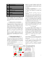
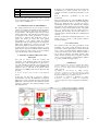
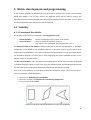
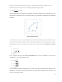
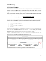
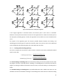
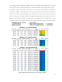
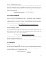
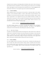
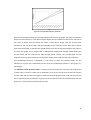
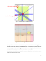
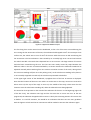
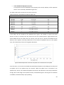
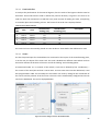
The user must enter the name of the zone and the coordinates of the four corners. Then for each
bordering line, the user has to determine where the zone is located against the position of the line.
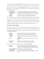
To facilitate this, the zone is displayed in a screenshot, and the current line is highlighted (in blue
on this screenshot). The instructions for the use of this tool are given in the lower left corner of the
window. In this example, the zone is located to the right of the current line, so the ‘greater than’
checkbox is chosen. This is repeated for the other three lines. Once all the steps in the tool have
been completed, the new zone is added to the ‘Zones’-sheet and can be used in the dashboard.
7.3.3.4
Available routes and intersections
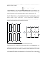
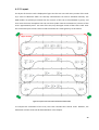
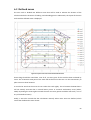
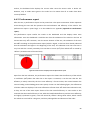
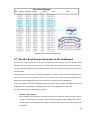
This last input is also connected to the layout of the manufacturing plant, or in this test, the layout
of the train track. To be able to calculate the efficiency of the train, Dijkstra’s Shortest Path
algorithm needs to be calculated. For this algorithm, a network or graph with the enclosed nodes
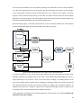
and edges needs to be defined. As seen under ‘4.2.1.1.2 Route efficiency’, a plant layout can be
translated to a network by translating every point of interest (loading-points, unloading-points,
intersections, etc.) to a node, and defining the edges ( = roads) that connect each node.
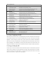
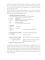
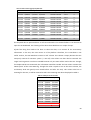
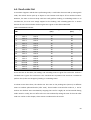
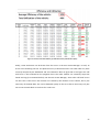
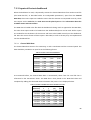
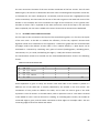
The network data needs to be entered into the ‘ShortestPathCalculations’-sheet in the following
format:
Table 13: Format of the network data
Node
0
1
2
3
4
X
1,8
3,1
4,5
5,1
6
Y Name Nbr. Of Edges 1st connection 2nd connection 3th connection
5,7
2
1
15
5,7 Lane 5
2
0
2
5,7
2
1
3
5,3 Lane 4
2
2
4
4,7
3
3
5
22
Some explanation is given to clarify this format: Each used node in the network is placed in a
different row of the table and is uniquely identified by the number in the first column. The
coordinates of every node are added in the table, and a name can also be given if the node
represents a zone of interest. In the table above, node 1 represents ‘Lane 5’. This node is situated
in the middle of ‘Lane 5’ and can be used as a loading- or unloading-point. Further, the number of
connected edges is given, and the nodes connected to those edges. For example node 1 has two
connecting edges that lead to node 0 and node 2.
68