Download MSMS 2.2 User`s Guide - Medical Device Development

MSMS User’s Manual
Medical Device Development Facility
Biomedical Engineering Department
University of Southern California
By:
Rahman Davoodi
Version 2.2
Table of Contents
1
2
3
General Information ........................................................................................................................... 10
1.1
Introduction ................................................................................................................................ 10
1.2
Minimum System Requirements ................................................................................................ 10
1.3
Installation Procedure ................................................................................................................. 10
1.4
Key Features................................................................................................................................ 10
Starting MSMS .................................................................................................................................... 11
2.1
Using Windows Shortcuts ........................................................................................................... 11
2.2
Using Command Line Interface ................................................................................................... 11
2.3
MSMS Graphic User Interface..................................................................................................... 12
2.4
Keyboard Shortcuts ..................................................................................................................... 13
Menus ................................................................................................................................................. 15
3.1
File Menu .................................................................................................................................... 15
3.1.1
New Model .......................................................................................................................... 15
3.1.2
Open .................................................................................................................................... 15
3.1.3
Reopen ................................................................................................................................ 16
3.1.4
Save ..................................................................................................................................... 16
3.1.5
Save As ................................................................................................................................ 16
3.1.6
Close .................................................................................................................................... 16
3.1.7
Preferences ......................................................................................................................... 16
3.1.7.1
General ............................................................................................................................ 17
3.1.7.2
Display ............................................................................................................................. 17
3.1.7.3
Framing ........................................................................................................................... 18
3.1.7.4
User ................................................................................................................................. 18
3.1.8
Import Model ...................................................................................................................... 18
2
3.1.8.1
Import SolidWorks Model ............................................................................................... 18
3.1.8.2
Import OpenSim Model .................................................................................................. 21
3.1.9
3.2
Exit....................................................................................................................................... 22
View Menu .................................................................................................................................. 23
3.2.1
Front .................................................................................................................................... 23
3.2.2
Back ..................................................................................................................................... 23
3.2.3
Right .................................................................................................................................... 23
3.2.4
Left ...................................................................................................................................... 23
3.2.5
Top ...................................................................................................................................... 24
3.2.6
Bottom (Under) ................................................................................................................... 24
3.2.7
Cameras .............................................................................................................................. 24
3.2.8
Camera Light On.................................................................................................................. 24
3.2.9
Default Lights On................................................................................................................. 24
3.2.10
View All ............................................................................................................................... 24
3.2.11
Full Screen ........................................................................................................................... 24
3.3
Model Menu ............................................................................................................................... 25
3.3.1
Show All Axes ...................................................................................................................... 25
3.3.2
Show Ground Axes .............................................................................................................. 25
3.3.3
Show Joint Controls............................................................................................................. 25
3.3.4
Hide Muscles ....................................................................................................................... 25
3.3.5
Hide Ligaments.................................................................................................................... 26
3.3.6
Hide Segments .................................................................................................................... 26
3.3.7
Hide Wrapping Objects ....................................................................................................... 26
3.3.8
Hide All Components .......................................................................................................... 26
3.3.9
Add Model........................................................................................................................... 26
3
3.3.10
Add Component .................................................................................................................. 26
3.3.11
Add Segment ....................................................................................................................... 27
3.3.12
Add Muscle ......................................................................................................................... 28
3.3.13
Add Ligament ...................................................................................................................... 31
3.3.14
Plot Anatomical Data for Muscles ....................................................................................... 33
3.3.15
Plot Anatomical Data for Ligaments ................................................................................... 34
3.3.16
Scale Segment ..................................................................................................................... 35
3.3.17
Model Info ........................................................................................................................... 36
3.4
Simulation Menu ......................................................................................................................... 37
3.4.1
3.4.1.1
General ............................................................................................................................ 37
3.4.1.2
Setup ............................................................................................................................... 38
3.4.1.3
Solver............................................................................................................................... 38
3.4.1.4
Dynamic Engine ............................................................................................................... 39
3.4.1.5
Output Data .................................................................................................................... 39
3.4.2
3.5
Simulation Setup ................................................................................................................. 37
Convert to Simulink ............................................................................................................. 40
Animation Menu ......................................................................................................................... 42
3.5.1
Setup ................................................................................................................................... 42
3.5.2
Start ..................................................................................................................................... 44
3.5.3
Pause ................................................................................................................................... 44
3.5.4
Stop ..................................................................................................................................... 44
3.5.5
Parse ADL File ...................................................................................................................... 44
3.5.6
Write Motion File ................................................................................................................ 44
3.5.7
Display Rendering Stats...................................................................................................... 44
3.5.8
Toggle Rendering Stats Display (Hz or ms).......................................................................... 44
4
3.6
4
Help Menu................................................................................................................................... 45
3.6.1
MSMS User Guide ............................................................................................................... 45
3.6.2
Report Bug .......................................................................................................................... 45
3.6.3
Request Feature .................................................................................................................. 45
3.6.4
MSMS Web Page ................................................................................................................. 45
3.6.5
MSMS Discussion Group ..................................................................................................... 45
3.6.6
About MSMS ....................................................................................................................... 45
Component Property Panels .............................................................................................................. 46
4.1
Segment ...................................................................................................................................... 46
4.1.1
General ................................................................................................................................ 46
4.1.2
Inertia .................................................................................................................................. 46
4.1.3
Material ............................................................................................................................... 47
4.1.4
Image................................................................................................................................... 49
4.1.5
Image Editing Window ........................................................................................................ 52
4.2
Joint ............................................................................................................................................. 56
4.2.1
General ................................................................................................................................ 56
4.2.2
Segments ............................................................................................................................. 57
4.2.3
Axes ..................................................................................................................................... 58
4.2.4
Motion................................................................................................................................. 59
4.2.5
Passive Joint Moment ......................................................................................................... 60
4.2.6
Image................................................................................................................................... 60
4.3
Muscle ......................................................................................................................................... 61
4.3.1
General ................................................................................................................................ 61
4.3.2
Muscle Path......................................................................................................................... 62
4.3.3
Morphometry...................................................................................................................... 64
5
4.3.4
Fibers Types ........................................................................................................................ 65
4.3.5
Fibers Properties ................................................................................................................. 66
4.3.6
Image................................................................................................................................... 68
4.4
Ligament...................................................................................................................................... 69
4.4.1
General ................................................................................................................................ 69
4.4.2
Ligament Path ..................................................................................................................... 70
4.4.3
Morphometry...................................................................................................................... 71
4.4.4
Image................................................................................................................................... 71
4.5
Wrapping Object ......................................................................................................................... 72
4.5.1
General ................................................................................................................................ 72
4.5.2
Type ..................................................................................................................................... 72
4.5.3
Pos. & Ori. ........................................................................................................................... 73
4.5.4
Path Components................................................................................................................ 73
4.5.5
Image................................................................................................................................... 74
4.6
Kinematic Driver.......................................................................................................................... 75
4.6.1
General ................................................................................................................................ 75
4.6.2
Attachments ........................................................................................................................ 75
4.6.3
Image................................................................................................................................... 75
4.7
Motor .......................................................................................................................................... 76
4.7.1
General ................................................................................................................................ 76
4.7.2
Attachments ........................................................................................................................ 76
4.7.3
Mass Props .......................................................................................................................... 77
4.7.4
Control Props ...................................................................................................................... 77
4.7.5
Electrical Props .................................................................................................................... 78
4.7.6
Mechanical Props ................................................................................................................ 78
6
4.7.7
4.8
General ................................................................................................................................ 79
4.8.2
Attachment ......................................................................................................................... 79
4.8.3
Image................................................................................................................................... 79
Camera ........................................................................................................................................ 80
4.9.1
General ................................................................................................................................ 80
4.9.2
Position & Orientation ........................................................................................................ 80
4.9.3
Frustum ............................................................................................................................... 81
4.10
Light............................................................................................................................................. 82
4.10.1
General ................................................................................................................................ 82
4.10.2
Position & Direction ............................................................................................................ 83
4.10.3
Color .................................................................................................................................... 84
4.10.4
Misc ..................................................................................................................................... 85
Appendix A: Motion File Formats ...................................................................................................... 86
5.1
MSMS Motion File Format (.msm) .............................................................................................. 86
5.1.1
Format of the header row ................................................................................................... 86
5.1.2
Format of the data rows ..................................................................................................... 87
5.1.3
An Example msm Motion File ............................................................................................. 88
5.2
6
Position Sensor............................................................................................................................ 79
4.8.1
4.9
5
Image................................................................................................................................... 78
SIMM Motion File Format (.mot) ................................................................................................ 89
Appendix B: Protocol for Live Animation (Feature Commands) ........................................................ 90
6.1
Ordered Joint Angles................................................................................................................... 90
6.2
Feature Commands ..................................................................................................................... 90
6.2.1
Packet Protocol for Feature Commands ............................................................................. 91
6.2.2
Example UDP Packets for Feature Commands ................................................................... 95
7
7
8
Appendix C: Animation of ADL in PowerPoint ................................................................................... 97
7.1
Using MSMS and PowerPoint to Animate ADL movements ....................................................... 97
7.2
MSMS model ............................................................................................................................... 97
7.3
Library of the motion files........................................................................................................... 97
7.4
ADL Animation Sequences .......................................................................................................... 98
7.5
Rules and Guidelines for Creation of ADL sequence in PowerPoint ......................................... 100
Appendix D: Muscle Model (Virtual Muscle) ................................................................................... 101
8.1
8.1.1
Fiber type level .................................................................................................................. 103
8.1.2
Whole muscle level ........................................................................................................... 103
8.1.3
Interactions with Neural and Skeletal Elements ............................................................... 104
8.1.4
Summary of Virtual Muscle’s formulations ...................................................................... 105
8.2
9
Structure of the Model ............................................................................................................. 102
Recruitment type ...................................................................................................................... 106
8.2.1
Natural Units ..................................................................................................................... 107
8.2.2
Apportioning PCSA among motor units ............................................................................ 108
8.2.3
Multiple motor unit recruitment behavior ....................................................................... 109
8.2.4
Lumped Units .................................................................................................................... 110
8.2.5
Intramuscular FES ............................................................................................................. 111
8.3
Energetics .................................................................................................................................. 112
8.4
Proprioception .......................................................................................................................... 112
8.5
Tips for obtaining morphometric measures ............................................................................. 112
8.6
References ................................................................................................................................ 115
Appendix E: MSMS Files and Directory Structure ............................................................................ 117
9.1
Model Directory ........................................................................................................................ 117
9.2
Common Image Directory ......................................................................................................... 118
8
9.3
Workspace.xml.......................................................................................................................... 118
10
Appendix F: MSMS Lights ................................................................................................................. 119
11
Appendix G: Collision and Contact ................................................................................................... 121
12
Appendix H: Special Features ........................................................................................................... 124
13
12.1
Blanking the model screen........................................................................................................ 124
12.2
Writing animation events to file ............................................................................................... 124
Appendix H: Revision Log ................................................................................................................. 126
9
1 General Information
1.1 Introduction
MSMS is a software application for modeling and simulation of neural prostheses systems. It can be
used to model and simulate human and prosthetic limbs and the task environment they operate in. The
simulations can be executed in a standalone computer to develop and test neural control systems or in a
virtual reality environment where the human or animal subject can interact with and therefore affect
the behavior of the simulated limb.
If you are new to MSMS, start with the tutorials where you will learn about the basic tools and features
in MSMS. You can find the tutorials in your MSMS installation folder. In chapter 3, you will learn about
all of the menus and their typical usage. In chapter 4, the graphic user interface for editing the
properties of the MSMS model components are described. Finally, the Appendices provide more
detailed information on important MSMS features and capabilities.
To see what is new in this version of MSMS, see the revision log in Appendix H.
1.2 Minimum System Requirements




Operating system: Windows XP, Windows 7 32-bit, Windows 7 64-bit.
512MB of RAM or higher.
Processor speed of 1.2GHz or higher recommended.
Graphic card with 512 MB or higher. For stereoscopic display, 3D stereo graphic cards are
available from NVIDIA and ATI.
1.3 Installation Procedure
MSMS is distributed through a single compressed zip file. To install MSMS, unzip the compressed file to
get the executable installer. Then run the installer and follow the instructions.
1.4 Key Features






Interactive tools for building and validation of human and prosthetic limbs and models of the
objects in the task environment
Tools for importing existing models from OpenSim, SIMM, and SolidWorks
Tools for physics-based simulations in Simulink
Tools for simulations in real-time virtual reality environments with the subject in the loop
Tools for animation of models off-line or in real-time
Tools for building animations of activities of daily life in PowerPoint
10
2 Starting MSMS
2.1 Using Windows Shortcuts
Click on the MSMS shortcut in Windows start menu.
2.2 Using Command Line Interface
To run MSMS from command-line, use the following syntax:
runmsms “Model Folder” A Live_Data Stereo_3D Fullscreen “Installation Folder”
Where,
“Model Folder” = Directory name where the MSMS model resides (directory name must be in quotes)
A
= Tells MSMS to start in Feature Command animation mode
Live_Data = Controls head-tracking mode (use arguments ON or OFF)
Stereo_3D = Controls stereo mode (use arguments ON or OFF)
Fullscreen = Controls full-screen mode (use arguments ON or OFF)
“Installation Folder” = MSMS installation folder
Example:
runmsms "c:\models\mymodel" a on off off “C:\MSMS\MSMS 1.0”
NOTE: The command line is designed primarily to quickly put MSMS in animation mode so that it can
receive and animate the motion data from the UDP port. In this mode, some editing functions may not
function properly. Therefore, if you plan on editing your model, start MSMS from Windows start menu.
11
2.3 MSMS Graphic User Interface
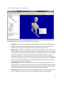
The MSMS graphic user interface consists of the following sections:





Menu Bar located at the top of the MSMS window, and gives access to most MSMS features.
Toolbar is located just below the Menu Bar and gives access to the most frequently used
features such as opening and saving models or choosing the background color.
Model Explorer lists all of the components in the opened model. The list can be viewed in four
different ways by clicking on one of the four buttons on the Model Explorer. Once a component
is selected in the top Pane, its attached components are displayed in the bottom Pane. Double
clicking on a component’s name will bring up its properties dialog box. Right clicking on a
component will bring up a menu with options to edit, remove, show, or hide the component.
There are also options to show only or show all components of the same type. If the component
does not have a visual representation in the model window (e.g. joints), the right-click menu
options will be limited to edit and remove.
3D Model Window is where the MSMS models are visualized, edited and animated. Here,
double clicking on a component’s name will bring up its properties dialog box. Right clicking on a
component will bring up a menu with options to edit, remove, show, or hide the component.
There are also options to show only or show all components of the same type.
Status Bar displays properties of muscles and wrapping objects when they are edited. In other
times, it displays the commonly used shortcuts for model manipulation and navigation.
12
2.4 Keyboard Shortcuts
Keyboard Shortcuts allow you to quickly perform important functions in the menus and navigate the
model in 3D window.
When you move your mouse over the buttons in the toolbar, you will see a text that shows the
equivalent keyboard shortcut for that button.
For the model window shortcuts to work, you have to click on the 3D model window to bring it to focus.
Here is the list of keyboard shortcuts:
Keyboard Shortcuts:




CTRL + O
CTRL + S
CTRL + Alt + S
CTRL + C









SHIFT + F – view front
SHIFT + B – view back
SHIFT + R – view right
SHIFT + L – view left
SHIFT + T – view top
SHIFT + U – view bottom
SHIFT + A – View all
SHIFT + S – Full screen
Esc
– Exit full screen





CTRL + Shift + M – Add Model
CTRL + Shift + N – Add component
CTRL + Shift + X – Add segment
CTRL + Shift + P – Add muscle
CTRL + Shift + Q – Add ligament


CTRL + Alt + C – Simulation setup
CTRL + Alt + E – Convert to Simulink




CTRL + Shift + C – Setup animation
CTRL + Shift + G – Start Animation
CTRL + Shift + H – Pause animation
CTRL + Shift + V – Stop animation


CTRL + Shift + J – Display Rendering Stats
CTRL + Shift + K – Toggle Rendering Stats Display (Hz or ms)
– Open
– Save
– Save As
– Close
13


SHIFT + LeftClick on Background + Drag – Move model in screen
ALT + LeftClick on Background + Drag – Rotate model in screen




SHIFT + UpArrow (CTRL + U, u)
SHIFT + DnArrow (CTRL + D, d)
SHIFT + LtArrow (CTRL + L, l)
SHIFT + RtArrow (CTRL + R, r)



Alt + Up/Dn Arrow
Alt + Lt/Rt Arrow
t, CTRL + t


i, SHIFT + i (mouse wheel) – Zoom in
o, SHIFT + o (mouse wheel) – Zoom out
– Move model up
– Move model down
– Move model left
– Move model right
– Rotate model about screen’s vertical axis
– Rotate model about screen’s horizontal axis
– Rotate model about screen’s normal axis
14
3 Menus
3.1 File Menu
3.1.1 New Model
This command creates an empty model, i.e. a model with no components. Once you have created a
new model, you can add components such as segments and muscles to complete it.
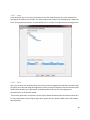
3.1.2 Open
This command loads an existing MSMS model from the disk drive. A MSMS model is stored in a directory
whose name is the name of the MSMS model. The model directory has a number of required and
optional sub-directories and files that are described in Appendix E.
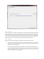
To open a MSMS model, click on File > Open to bring up the model browser window. Here, you must
choose the model directory where your model resides by double-clicking on it or selecting it and clicking
on “Open” to open it. In the model browser, the directories that contain a valid MSMS model (with
proper subfolders and model files) are displayed with an MSMS icon indicating that they are valid MSMS
models and can be opened by MSMS.
15
Note: When MSMS opens a model, it searches model's local image folder for segment images first. If it
couldn't find all of the images required by the model, it will then search the common image library (set
in "File>>Preferences>>General"). If the common image library folder is wrong (e.g. "C:\" instead of
"C:\users\models\images"), MSMS will search C:\ and all of its subfolders for the images. Depending on
the size of the image folder, the search could take a very long time. When this happens, pay attention to
the progress window that is displayed while opening a model. In progress window, MSMS displays the
image folders it is currently searching for the images. If you notice that the wrong folders are being
searched, change the image library path in "File>>Preferences>>General".
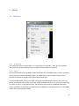
3.1.3 Reopen
This command provides a list of five recently opened models and allows the user to quickly open one of
them.
3.1.4 Save
This command saves the changes to the model.
3.1.5 Save As
This command saves changes to the model under a different name or the same name at another
location on disk. If the model contains images that are not stored in the MSMS Image Library folder,
these images are copied to the new model location. Furthermore, if the “Save Main Library Images”
option is checked, even the images located in the Image Library are copied to the new model location.
When MSMS loads a model, it searches for the required images in the local model folder and the main
image library (specified in the File >> Preferences). This allows you to keep large image files in the main
library and reuse them in many models. But if you like to share your model with others or open them in
a different computer, you have two choices. You can share your image folder along with the model or
make sure that all required images are saved in the model’s local folder (by selecting “Save Main Library
Images”).
3.1.6 Close
This command closes the model in MSMS workspace.
3.1.7 Preferences
Preferences setup allows you to specify the location of your image library, the background color, and the
2D and 3D displays. Preferences Setup includes four tabs.
16
3.1.7.1 General
In the General tab you can change or set the path for the common image folder. When loading a model,
MSMS first searches the model's local image folder for the required images (3D meshes and textures).
But if it couldn't find all of the images in the local image folder, it will search the common image folder
and its subfolders. When loading the model, the progress window displays the folders searched for the
images. In this tab, you can also change the background color of the 3D model window.
3.1.7.2 Display
MSMS supports both 2D and 3D displays. In the Display Tab the following can be edited:

The number of screens that the display contains. This would be required in case of head mount
displays or multi-projection displays both of which have multiple screens and the user needs to
configure each screen individually.

The monoscopic view needs to be set in some cases, for example, a head mount display that
gets its left and right feed from two different video channels. In that case, you cannot get stereo
vision by just enabling stereo 3D. Instead you need to set the monoscopic view of one screen to
“Left Eye” and the other screen to “Right Eye”.
17
3.1.7.3 Framing
The Framing Tab controls aspects specific to how the MSMS window affects the view as seen by the
user. Based upon the settings, the view frustum gets modified.
3.1.7.4 User
The User tab is used to control settings that are user dependant, e.g. the position of eyes. When the
physical to virtual eye correspondence is set to “Virtual Eye is at viewable distance from point of
interest”, the eye position will need to be specified with respect to the screen and not with respect to
the head. The title text “Eye Position with respect to Head” will change to “Eye Position with respect to
Image Plate” to reflect this.
3.1.8
Import Model
3.1.8.1 Import SolidWorks Model
This command imports a SolidWorks model into MSMS. MSMS allows importing CAD designs from
SolidWorks. This process is as follows.
Engineers can build accurate models of prosthetic limbs in SolidWorks and automatically convert it to a
Physical Modeling XML file. This conversion is done in the SolidWorks environment using the CAD-toSimMechanics translator, a free add-on utility available from Mathworks website. The Physical Modeling
XML file can be read into SimMechanics to dynamically simulate the prosthetic limb. The same file can
also be read into MSMS to represent the prosthetic limb in MSMS. No MATLAB component is required
at any time to perform the import to MSMS.
The Physical Modeling XML includes bodies to represent the assembly’s parts and maps the constraints
between the parts into joints. The ‘Part’, the ‘Constraints’ (or mates), the ‘Fundamental Root’ and the
‘Subassembly’ Solidworks components correspond respectively to the ‘Body’, the ‘Joints’, the ‘GroundRoot Weld-Root Body’ and the ‘Subsystem’ in SimMechanics. After importing the prosthetic limb model
18
into MSMS, it can be populated with components such as actuators and sensors, it can be attached to a
human model in MSMS, and it can be simulated within an appropriate task environment.
In its import process, MSMS also uses STL files exported from SolidWorks to properly visualize the
prosthetic limb segments. Therefore, MSMS integrates a complete set of information directly available
from the SolidWorks CAD design software: the assembly and its visualization. The process should be
completely automatic and the user should not have to modify the linkage manually in the XML file. This
aspect of the translation guarantees the data has not been corrupted.
Because conversion from CAD to SimMechanics involves interpretations of what each element in the
CAD model is and how it has to be represented in SimMechanics, Mathworks provides guidance and
instructions on configuration and export of your CAD model so that it can be successfully imported into
SimMechanics. You can find these guidelines in MathWorks web site at:
http://www.mathworks.com/access/helpdesk/help/toolbox/physmod/mech/
Further, current MSMS tools for importing CAD models do not handle all system topologies, which
imposes additional constraints on importable CAD models. For example:




The MSMS converter does not yet handle closed loop mechanical systems and subassemblies. If
the SolidWorks model includes a closed loop system or a subassembly, it cannot get converted
to MSMS. Subassemblies can be avoided in the model by bringing the parts and the constraints
contained in the subassembly to the higher hierarchical level. In other words, a flat assembly is
required: all parts are mated together at the top level.
The CAD assembly parts need to have masses and inertia tensors. This may be automatically
computed from density and geometry as long as all parts have material properties defined.
Unnecessary constraints must be avoided because they are translated into many weld joints
that complicate the simulation model but are not necessary.
Only the complete assembly can be exported to XML and not a part of it.
Finally, the user must export the segment images from the CAD model. MSMS uses these images to
visualize the imported CAD model. The following rules will ensure that the images are exported
properly.


A ‘Coarse’ resolution is sufficient for visualization purposes. STL files have very high resolution
because they are meant to be used for manufacturing (stereolithography). MSMS reads directly
the STL format. However, this format describes only surface geometry of 3D objects and does
not include any information about color or texture. It can be useful to convert the STL files to
the OBJ format and then include color and texture properties.
Set the ‘Output’ parameter to binary. ASCII STL files can quickly become very large. Therefore,
the binary STL is a better option.
19


Set the ‘Units’ to meters. The MSMS environment uses metric units and the STL format does not
include any information about the units even though the unit may be specified in the comments
in the STL file.
Check “Do not translate STL output data to positive space”. For manufacturing, vertices’
coordinates will be converted to positive space. However, in MSMS, it is important to keep the
coordinates as they are to preserve the concordance between the images and the Physical
Modeling XML file.
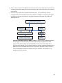
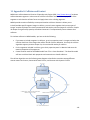
SolidWorks Model of Prosthesis
Actuator & Sensor Data
Human Model Data
World Model Data
STL Files
Physical Modeling
XML File
MSMS
Matlab
SimMechanics
Simulink Model of
Prosthesis + Human + World
Simulink Model of
Prosthesis
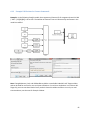
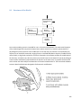
Importing a SolidWorks model to MSMS: SolidWorks outputs a Physical Modeling XML file
describing the mechanical linkage and STL files representing the appearance of each
segment. Both sets of outputs are used by MSMS to create an accurate model of the
prosthetic limb in MSMS. The final Simulink model can be built via Matlab/SimMechanics or
MSMS. But the use of MSMS allows the users to attach the imported prosthetic limb to a
human, add additional prosthetic components such as actuators, and simulate it in an
appropriate task environment.
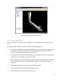
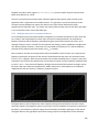
20
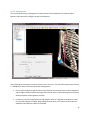
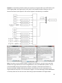
A prosthetic limb imported from SolidWorks
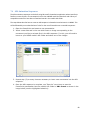
3.1.8.2 Import OpenSim Model
This command imports an OpenSim model into MSMS. The Open dialog shows only OpenSim model
files.
To successfully import models from OpenSim, follow the following guidelines:

Open and save the OpenSim model with the OpenSim version 2.2.0 or higher. To save, you must
use “Save As” and select a name that is different from the original model name. Otherwise,
OpenSim will not upgrade the model to the newer format.

The 3D shapes of the segments (.vtp files) required by the model must all be in a folder named
"Geometry" in the same folder as the OpenSim model.

When there are no equivalent components in MSMS, the imported components are mapped to
the closest MSMS component as described below. If necessary, you can edit these after
importing.

Ellipsoid wrapping object is converted to spherical wrapping object.

Torus wrapping object is converted to Ring wrapping object.

Muscle via points are converted to muscle fixed points.
21

When the functions for the coordinates of the moving point are nonlinear, they are converted to
linear functions.

Tendon slack length is converted to optimal tendon length
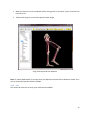
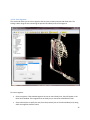
A leg model imported from OpenSim
Note: To import SIMM models, first import them into OpenSim and save them as OpenSim models. Then
you can import the OpenSim models to MSMS.
3.1.9 Exit
This command closes the currently open model and exits MSMS.
22
3.2 View Menu
3.2.1 Front
This command shows the Front view. Keyboard shortcut: Shift + F. The Front view is the Y-Z plane
projection of the model with Y axis pointing upwards, and Z axis pointing to the left of the screen.
3.2.2 Back
This command shows the Back view. Keyboard shortcut: Shift + B. The Back view is the Y-Z plane
projection of the model with Y axis pointing upwards, and Z axis pointing to the right of the screen.
3.2.3 Right
This command shows the Right view. Keyboard shortcut: Shift + R. The Right view is the Y-X plane
projection of the model with Y axis pointing upwards, and X axis pointing to the right of the screen.
3.2.4 Left
This command shows the Left view. Keyboard shortcut: Shift + L. The Left view is the Y-X plane
projection of the model with Y axis pointing upwards, and X axis pointing to the left of the screen.
23
3.2.5 Top
This command shows the Top view. Keyboard shortcut: Shift + T. The Top view is the X-Z plane
projection of the model with X axis pointing upwards, and Z axis pointing to the right of the screen.
3.2.6 Bottom (Under)
This command shows the Bottom view. Keyboard shortcut: Shift + U. The Bottom view is the X-Z plane
projection of the model with X axis pointing upwards, and Z axis pointing to the left of the screen.
3.2.7 Cameras
All models have a default camera for viewing the model. The user however, can create any number of
custom cameras for a model. All such cameras will be listed here and can be chosen as the active
camera by the user.
3.2.8 Camera Light On
This command toggles on and off the spotlight that is attached to the camera and always points in the
same direction as the camera.
3.2.9 Default Lights On
This menu option toggles on and off the default lights which is a combination of one ambient light and
two directional lights.
In addition to the camera and default lights, the user can add new lights. Lighting of the MSMS “world”
can be accomplished by four basic types of light: (1) ambient, (2) directional, (3) point, and (4) spotlight.
3.2.10 View All
This menu option redirects the camera toward the model and moves it back until the whole model can
be seen. This is useful when the camera is pointing to the wrong direction and the model is invisible.
3.2.11 Full Screen
This menu option enlarges the 3D window to cover the entire screen. The keyboard shortcut for this
command is Shift + S. You can press Esc to get back to the normal screen mode.
24
3.3 Model Menu
Includes tools for building and editing of models.
3.3.1 Show All Axes
Shows/hides the local reference frame of all components.
3.3.2 Show Ground Axes
Shows/hides Ground reference frame.
3.3.3 Show Joint Controls
Shows/hides joint controls for all joint degrees of freedom in the model. To facilitate finding the desired
degree of freedom in large models, the names of the degrees of freedom are sorted in alphabetical
order. You can these sliders to control the motion of the individual joint degrees of freedom in the
model.
3.3.4 Hide Muscles
Shows/hides all muscles.
25
3.3.5 Hide Ligaments
Shows/hides all ligaments.
3.3.6 Hide Segments
Shows/hides all segments.
3.3.7 Hide Wrapping Objects
Shows/hides all wrapping objects.
3.3.8 Hide All Components
Shows/hides all model components.
3.3.9 Add Model
Using this command, one can add an entire human, prosthesis, or world assembly to the current model.
To add, you must browse to the XML file of the desired assembly (human.xml, prosthesis.xml, or
world.xml) and add it to your model. For example, you can remove a prosthesis in the model and add a
different one to replace it. This allows you to combine a human model with various prosthesis and world
models to quickly build different task models.
3.3.10 Add Component
Brings up the add component wizard that allows you to add any model component supported by MSMS.
Joints are automatically created when you create a segment. Once a component is inserted, it will show
up in the model explorer as the currently selected component.
The newly created component may belong to one of the Human, Prosthesis, or World Category. If you
attach the new component to an existing component, it will inherit its parent’s category by default. If
you are adding a component to a new blank model, it will assume Human Category by default. If this is
not desirable, open the component’s GUI after its creation and change its category.
26
Note: Add Component tool collects only the most basic information to quickly add new components to
the model. It therefore does not allow you to edit all parameters of the component while it is added to
the model. For Segments (and joints), Muscles, and Ligaments, there are interactive wizards that give
you more control over the parameters of the added component (see below). In addition, all parameters
of the new components can be edited later from their properties panel.
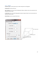
3.3.11 Add Segment
This command will bring up the segment creation wizard. The wizard allows you to quickly build a
segment/joint pair and interactively configure its properties.
27
In the wizard, you must specify the parent segment where the new segment will attach to, the name
and the type of the joint between the parent segment and the new segment, the joint offset from the
parent segment, and the shape of the new segment.
If a segment in the model is already highlighted (selected), Add segment will use it as the parent for the
new segment.
Don’t worry if the shape of the new segment does not have the desired position, orientation or the
material properties. You can edit these later in the new segment’s property panel.
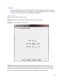
3.3.12 Add Muscle
This command will bring up the muscle creation wizard. The wizard allows you to quickly add a muscle
and interactively configure its path and properties.
28
After selecting this command, the cursor will turn into a red cursor. To interactively create the muscle,
you have to:

Click to select origin then drag as red line and release at the insertion point to create a muscle
with straight line path between the origin and insertion points. A panel showing the current and
default morphometric properties of the muscle will open.

If necessary, click on the muscle path and drag to a point on a segment and release to create
new via point. Repeat as needed. While adding new via points, the contents of the muscle
properties window will be update to reflect the new path.

If necessary, click on a wrapping object and then click on a muscle segment. This associates the
wrapping object with that segment of the muscle. Repeat as needed. While adding wrapping
objects to the path, the contents of the muscle properties window will be update to reflect the
new path.
29

Once the desired path is drawn, enter the remaining morphometric parameters and click Apply.
Use the current muscle lengths as a guide to come up with reasonable values for optimal muscle
and tendon lengths and the mass. Click OK to close the Morphometry window. This will bring up
the Fiber Types window.

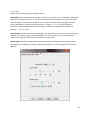
In the Fiber Types window, select whether you want the muscle model to output energy
consumption or model proprioceptive sensors (muscle spindles and Golgi tendon organs), select
the recruitment type, and the muscle fascicle’s fiber composition. Click OK to complete the
muscle creation wizard and create the new muscle.
30
3.3.13 Add Ligament
This command will bring up the ligament creation wizard. The wizard allows you to quickly add a
ligament and interactively configure its path and properties.
After selecting this command, the cursor will turn into a red cursor. You can follow steps similar to those
in “Add Muscle” above to interactively create new ligaments:

Click to select origin then drag as red line and release at the insertion point to create a ligament
with straight line path between the origin and insertion points. A panel showing the current and
default properties of the ligament will open.

If necessary, click on the ligament path and drag to a point on a segment and release to create
new via point. Repeat as needed. While adding new via points, the contents of the properties
window will be update to reflect the new path.
31

If necessary, click on a wrapping object and then click on a ligament segment. This associates the
wrapping object with that segment of the ligament. Repeat as needed. While adding wrapping
objects to the path, the contents of the properties window will be update to reflect the new
path.

Once the desired path is drawn, enter the remaining parameters. Use the current ligament
lengths as a guide to come up with reasonable values for the resting length. Click OK to
complete the ligament creation wizard and create the new ligament.
32
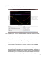
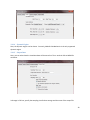
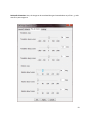
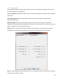
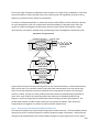
3.3.14 Plot Anatomical Data for Muscles
This command will open the anatomical data plotter for muscles.
Here, you can plot muscles’ anatomical data in the model and compare them with the experimentally
measured data. To plot new curves:

Inside the Y-Axis box, select the muscle attribute you want to plot and the muscles for which
you want to plot these attributes for.

Inside the X-Axis box, select the joint degree of freedom against which you want to plot the
muscle attributes. Also select the increments for the joint angle.

Click “Add Curves” to plot the data. This will add the new curves to the plot area, add the
corresponding legends, and add the names of the new curves to the “Curve List” window.
Please note that:

At any time, you can right click on the plot area and select “Import from file” to import
experimentally measured data or data previously exported from the plotter. The imported file
must be a text file with the following format. The header row includes the name of the degree
of freedom against which all muscle attributes are to be plotted followed by the names of the
muscle attributes. There must be only one degree of freedom name (which signify the X-axis)
33
but there is no limit on the number of the muscle attributes (which signify the Y-axis variables).
The data rows contain the data corresponding to the variables in the header.
Joint_DOF
Attribute_1
Attribute_2
….
0
0.50
200
…
0.1
0.52
210
…
0.2
0.55
215
…
…
…
…
…

At any time, you can right click on the plot area and select “Export to file” to save the curves to a
text file. The exported files follow the format of the imported files. If the data in the current plot
contains more than one X-axis variable, the data will be exported into multiple files, each
containing only one X-variable.

You can select one or more curves form the “Curve list” and click Remove to delete them from
the plot.

Clicking on “Clear” deletes all the curves in the plot.

You should select the increment for the X-Axis with care. Large increment reduces the data
points that must be calculated and is faster. But the curves will not be smooth. More
importantly, the moment arm and moment curves that require numerical differentiation of the
muscle length will be noisy. A very small increment on the other hand may take a long time to
plot because many more data points must be calculated. So, use the default value for the
increment unless it produces noise curves or takes too long to plot.
3.3.15 Plot Anatomical Data for Ligaments
This command will open the anatomical data plotter for ligaments. The operation of the ligament plotter
is similar to the muscle plotter (see section 3.3.14 above).
34
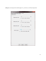
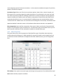
3.3.16 Scale Segment
This command allows you to scale a segment that has joints on both proximal and distal ends. The
scaling is done along the axis connecting the proximal and distal joints of the segment.
To scale a segment:

Select a segment. If the selected segment has one or more distal joints, they will appear in the
Distal Joints window. If the segment has no distal joint, it cannot be scaled with this tool.

Select a distal joint to specify the axis (from the proximal joint to the selected distal joint) along
which the segment must be scaled.
35

Enter a scale factor for the segment and click OK to scale the segment
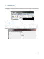
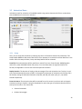
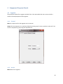
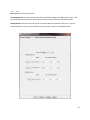
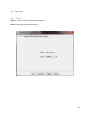
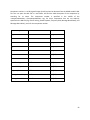
3.3.17 Model Info
This menu option allows you to obtain component ID numbers and the joint sequence numbers.
When developing a simulation program in Simulink or other environments to send Feature commands
to MSMS, the user needs to know the component IDs and the joint sequence numbers. These numbers
are available in the model XML files and can be obtained by opening them in a text editor and searching
for the IDs and the sequence numbers. But this process is time consuming and inconvenient.
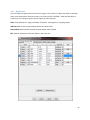
The Model Info menu options allow you to display the component IDs in the Model Explorer or write
model IDs or the joint sequence numbers into a text file in an easy to read tabular format.
36
3.4 Simulation Menu
Includes tools for setting up and creation of a Simulink model to simulate the physics-based movement
of the MSMS model.
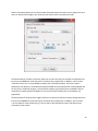
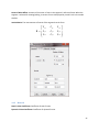
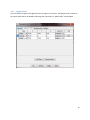
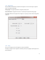
3.4.1 Simulation Setup
The Simulation Setup allows you to setup the simulation configuration before exporting it to Simulink.
3.4.1.1 General
Here, you can set the gravity vector for physics-based simulation. The default gravity vector (0 -9.81 0)
should not be changed unless the simulated movements occur on the Space station or the moon!
37
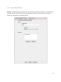
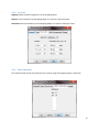
3.4.1.2 Setup
In the setup tab, you can see the tree structure view of the model and enter the initial conditions for
each degree of freedom in the model. The initial positions are initially set to the default joint angles (set
in the Joint properties panel) but can be modified here to simulate the model from any starting posture.
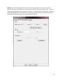
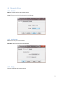
3.4.1.3 Solver
Here, you can select the simulation time, the type of numerical integration (Fixed-step or Variable-step),
the type of the numerical integration algorithm, and the numerical integration step sizes and tolerances.
These will be passed to the automatically created Simulink model. You can also change these
parameters later in the Simulink model.
These solver parameters are important for the physics-based simulation and must be chosen with care.
For more information on choosing the right solver options for your specific model, consult the Simulink
documentation.
38
3.4.1.4 Dynamic Engine
Here, the dynamic engine can be chosen. Currently, Matlab’s SimMechanics is the only supported
dynamic engine.
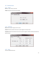
3.4.1.5 Output Data
Here, you can select how the simulation data will be stored in a file or send via UDP to MSMS for
animation.
In Storage In File box, specify the sampling time for data storage and the name of the output file.
39
In Live Animation box, select the sampling time for sending the live motion data, the method for sending
the motion data (via MSMS UDP Block or xPC UDP Block), and the type of protocol for packaging the
motion data (Feature Commands or Joint Angles).
MSMS UDP Block works even if you don’t have xPC Target toolbox. But “xPC UDP Block” requires xPC
Target toolbox. If you plan on executing the simulation in real-time xPC Target PC, you must use “xPC
UDP Block”. If you don’t have this toolbox or you don’t want to run the simulations in a real-time target,
you can use “MSMS UDP Block”.
The animation data can be packaged using two different protocols: Feature Commands and Joint Angles.
The Joint Angles format can be used to send only the joint motions but Feature Commands is a more
comprehensive format and can be used to send not only the joint motions but also commands to control
the VR simulations such as sound playback, drawing trajectories, changing the color or size of objects,
etc. For more see Appendix B.
3.4.2 Convert to Simulink
This command saves a Simulink simulation model (.mdl) in the model’s Matlab folder. This simulation
model represents the algorithms that can simulate the movement of the MSMS model in response to
control excitations and external forces.
You can open and run the Simulink model in Matlab’s Simulink program. When executed, the simulation
model will generate motion data that are sent to MSMS via UDP for on-line animation. To view the
simulated motion in MSMS while the simulation is running in Simulink, you need to setup and run the
animation from the Animation menu.
When the simulation ends or stopped by the user, the resulting motion data for the duration of
simulation are also saved in a MSMS-compatible msm motion file. This motion file can be loaded to
MSMS to animate the model off-line.
Notes:

To run the Simulink models, you have to add MSMS’s Matlab folder (e.g. C:\MSMS\MSMS
1.0\bin\Matlab) to the Matlab path (using File >> Set Path). In some operating systems, if you
want Matlab to remember the set path for future sessions, you have to run Matlab as
administrator to set the path (right click on Matlab shortcut and choose "Run as administrator").
This setup has to be done once after a new MSMS installation.

Usually after creating a Simulink model, you will add other Simulink blocks to the model to
provide inputs to the model or display the results. If you make such changes by adding your
user blocks, "Save Simulation" will give you the option to keep or overwrite your changes. This
option can be very useful if you make frequent changes to your MSMS model and create new
Simulink blocks but you don't want to add the user blocks every time you do it. If you choose to
keep your changes, MSMS will overwrite the blocks that it usually generates and will keep the
40
user blocks intact. If you choose not to keep your changes, MSMS will delete the user blocks
from the Simulink model.
41
3.5 Animation Menu
Includes the tools for animation of the MSMS models using motion data stored in files or motion data
sent to MSMS via a live source in real-time.
3.5.1 Setup
Here, you can setup the animation by selecting the source of animation data and its parameters. This
setup enables MSMS to load motion data from a file or prepares it to receive the motion data from a live
stream. After this setup the Start, Pause, ands Stop buttons will be activated.
From File: The animation data will be read from a motion file in one of two formats: SIMM/OpenSim
motion file (.mot) and MSMS motion file (.msm). For more information on supported motion file
formats, see Appendix A. You can also select the speed of animation.
Replay Duration: The duration of replay as the percentage of the real animation time. To play it in realtime, set the Animation Duration to 100%. For example if the duration of animation in the motion file is
10 seconds, setting the Animation Duration to 50, 100, and 400, will cause it play in 5, 10, and 40
seconds respectively.
From Live Source: The animation data will be received from a live source in real-time such as dynamic
simulation running in Simulink. Using the drop-down list select the type of simulation data that will be
sent by the live source. The choices are:

Feature Commands

Ordered Joint Angles
42
Feature Commands allows you to control model properties beyond its motion such as object sizes and
color etc. Ordered Joint Angles, only sends the joint motion data to animate the model.
The Edit window for Feature Commands, allows you to select the UDP port number through which the
live source and MSMS will send and receive animation data, respectively. In addition, you can select
“Show On-Screen Text” to setup MSMS to display text in 3D model window. The latter creates a
billboard for text display in 3D window and prepares MSMS to receive the position of the billboard and
the text from a simulation program. The simulation program (e.g Simulink) must use MSMS’s feature
commands to send these data to MSMS. To learn more on how to display text in 3D window, see
Appendix B.
The Edit window for Ordered Joint Angles, allows you to select the UDP port number through which the
live source and MSMS will send and receive animation data, respectively. In addition, you can select
“Use Live Data for Camera Positioning” if the live source will send data to control the position and
orientation of the camera.
43
3.5.2 Start
This command starts animation. It will be active after the animation is Setup.
3.5.3 Pause
This command pauses animation. It will be active after the animation is Setup.
3.5.4 Stop
This command stops animation. It will be active after the animation is Setup.
3.5.5 Parse ADL File
This command allows you to convert an animation sequence built in Microsoft PowerPoint to the msm
motion file format that can be animated in MSMS. For more details on how to build complex animation
sequences in PowerPoint, see Appendix C.
3.5.6 Write Motion File
This command allows MSMS to create a msm motion file with single frame of data corresponding to the
current posture of the model in MSMS.
There are two potential uses for these motion files. First, because these files have the correct motion file
format, they can be used as starting point to manually create new motion files. Second, motion files
created in the start and end postures of a movement can be used to create primitive motion files that
interpolate the frames in between these two postures. For more details, see Appendix C.
3.5.7 Display Rendering Stats
When a model is animated in MSMS, this command will display the rendering statistics in status bar. By
default, the rendering rates in Hz will be displayed. You can use this feature to see how fast MSMS and
your visualization PC can render a specific model. This evaluation can help you take actions such as
simplifying the model or acquiring faster video cards, if necessary, to animate your model in real-time.
3.5.8 Toggle Rendering Stats Display (Hz or ms)
This command toggles the display of the rendering statistics between rendering rates in Hz and
rendering periods in ms. For this command to work, the “Display Rendering Stats” command must be
selected first.
44
3.6 Help Menu
3.6.1 MSMS User Guide
This command opens this document.
3.6.2 Report Bug
This command opens your default email application and allows you to report MSMS bugs and defects to
the MSMS development team.
3.6.3 Request Feature
This command opens your default email application and allows you to request new MSMS features.
3.6.4 MSMS Web Page
This command opens the MSMS web page.
3.6.5 MSMS Discussion Group
This command displays information about MSMS discussion group MSMS-L.
3.6.6 About MSMS
This command displays information about MSMS and its developers.
45
4 Component Property Panels
4.1 Segment
The properties window for a segment includes 5 tabs. Each tab enables the user to view and edit a
number of related properties of the segment.
4.1.1 General
Name: A unique name for the segment such as humerus.
Group: All the components in a model are divided into three groups: human, prosthesis, and world. You
can set a component’s group using this drop-down list.
4.1.2 Inertia
Mass: Mass of the segment.
46
Center of Mass Offset: Location of the center of mass in the segment’s reference frame. When the
segment is selected for viewing/editing, its center of mass is displayed by a small circle in the model
window.
Inertia Matrix: The mass moment of inertia of the segment has the form:
 I xx

I   I yx

 I zx
I xy
I yy
I zy
I xz 

I yz 
I zz 

4.1.3 Material
Static Friction Coefficient: Coefficient of static friction.
Dynamic Friction Coefficient: Coefficient of dynamic friction.
47
Coefficient of Restitution: Coefficient of restitution is between 0 and 1 and determines the elasticity of
the segment. A value of 0 means that the segment is completely elastic (bouncy), while a value of 1
means that the segment is completely inelastic (sticky). Currently, this parameter is not used by MSMS's
collision algorithm.
Softness: Softness is a value between 0 and 1 and determines how deformable the segment is.
Currently, this parameter is not used by MSMS's collision algorithm.
Normal Force Spring Constant: Spring constant used to calculate the elastic component of the normal
collision force.
Normal Force Damping Constant: Damping constant used to calculate the damping component of the
normal collision force.
Friction Force Spring Constant: Spring constant used to calculate the elastic component of the static
friction force in contact.
Friction Force Damping Constant: Damping constant used to calculate the damping component of the
static friction force in contact.
To learn more about collisions in MSMS see Appendix G.
48
4.1.4 Image
To provide the maximum flexibility in designing the appearance of the segments, MSMS allows the users
to add any number of shapes to represent a segment. These shapes can be individually added, removed,
edited, and positioned on a segment.
By default, when you add a segment to your model using Add Component wizard, it does not have any
shapes attached to it. Therefore, you can see the newly added segment in the Model Explorer but not in
the 3D model window. You can design the appearance of your segment by adding image to your
segment. To add an image, double click on the new component name and edit its image properties in
the image tab. If you add a segment using the Add Segment wizard, you can add images to the segment
in a single step.
MSMS allow you to add two types of shapes to your segments: primitives and 3D meshes.
Primitives: Can be used in segments that have relatively simple appearance. The supported primitives
include cylinder, sphere, box, hemisphere, and capped cylinder. Because MSMS allows you to add any
number of shapes to each segment, you can combine multiple primitives to build more complex shapes,
if necessary. Once a primitive shape is added to a segment, all of its properties such as material
properties, its position and orientation with respect to the segment, and its scaling parameters can be
edited independent of any other shape attached to that segment. This provides the maximum flexibility
and enables the users to build segments with the desired appearance even with the use of simple
primitives.
3D Meshes: Can model any 3D shape and can be used to model the appearance of segments with
complex shapes such as human body segments, bones, and prosthetic limbs. To add a 3D mesh to a
segment, add a new image and select Mesh from the 3D Shape drop down menu. Then import the 3D
mesh by clicking on the Add button that will allow you to browse for the 3D mesh files. For complex
shapes made of multiple 3D meshes, you can either add more images to the segment each containing
one 3D mesh or you may add multiple 3D meshes to one image. In the later case, any editing to the
image will apply to all of the 3D meshes attached to it.
The 3D meshes may be in one of the many 3D file formats but the one that is completely supported by
the MSMS is OBJ file format. So, before importing to MSMS, you must first convert your 3D meshes to
OBJ file format, if needed.
Before adding 3D meshes to your segment, you must have created or obtained these 3D meshes. You
can obtain your 3D shapes by purchasing them from the 3D model vendors, by finding and downloading
them free of charge from the Internet, or by creating them yourself in a 3D modeling software such as
MAYA, 3ds Max, Blender, etc. These software tools allow you to create new 3D shapes, customize them
by editing their shape and texture, and perform file format conversion, when necessary.
49
Select: This checkbox toggles on and off the visibility of the image in the 3D pane.
Collision: This checkbox toggles on and off to indicate whether the image will be considered for collision
or not. In other software, you will have to apply collisions to the whole model or a group of segments.
But MSMS allows you to include/exclude individual images of segments in collision. This provides
maximum flexibility and could be very useful in optimizing the speed of simulations. For example you
can use a complex 3D mesh to represent the realistic features of the fingertip in MSMS and add a
simpler second image to the fingertip segment such as a sphere (whose collision detection is much
faster than 3D meshes) to handle its collision with other objects. You can hide this second image so that
it doesn't obstruct the realistic appearance of the segment. For more info on MSMS collision detection
and handling, see Appendix G.
Add: This command adds an image to the segment.
Edit: If clicked after selecting an image, it opens the image edit window to edit the selected image’s
properties (see below).
Remove: Deletes the selected image.
50
51
4.1.5
Image Editing Window
General: An image name can be chosen here. The name does not need to be unique. For the shape of a
3D image, there are five primitive choices and a general mesh choice. The primitives are: Cylinder,
Sphere, Box, Hemisphere, and Capped Cylinder.
52
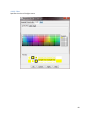
Material: Here, the object’s appearance can be set by choosing: Object color, Ambient, Diffuse,
Specular, Shininess, and Transparency. You can select an object’s color by clicking on “Pick”. The color
selected will be applied to all color types for the object, i.e., ambient, diffuse, and specular. Therefore, it
will be approximately the color of the object in all light types. Advanced users can select the color for
each individual color type by clicking on “Advanced Color Options”.
53
Position & Orientation: Here, the image can be translated along and rotated about any of the x, y, and z
axes of its parent segment.
54
Scaling: Here, the image can be scaled along any of x, y, and z axes, or uniformly along all axes.
55
4.2 Joint
The properties window for a joint includes 6 tabs. Each tab enables the user to view and edit a number
of related properties of the joint.
4.2.1 General
Name: A unique name for the joint such as: Elbow.
Group: All the components in a model are divided into three groups: human, prosthesis, and world. You
can set a component’s group using this drop-down list.
56
4.2.2 Segments
Proximal Segment Name: Selects the proximal segment for this joint.
Joint Center Offset: Sets the joint center offset in proximal segment’s local reference frame.
Distal Segment Name: Sets the distal segment for this joint.
57
4.2.3 Axes
Joint Type: Sets the type of the joint.
Translational Axes: Sets the name and axes of the translational degrees of freedom of the joint. Click
the numbered button next to the name field to set the minimum, maximum and default values.
Rotational Axes: Sets the name and axes of the rotation degrees of freedom of the joint. Click the
numbered button next to the name field to set the minimum, maximum and default values.
58
4.2.4
Motion
Translational Axes: The slider and numerical field allow you to move the joint along its translational
axes.
Rotational Axes: The slider and numerical field allow you to move the joint along its rotational axes.
59
4.2.5 Passive Joint Moment
Here you can specify the parameters of the passive joint moments for each degree of freedom in the
joint.
DOF Name: Select a degree of freedom from the drop-down list.
Damping Factor: Set a damping factor for the selected degree of freedom.
Low Limit: Check “Active” if you want the passive moments applied at the lower end of the joint’s
motion. Select a torque function for calculation of the passive joint moment and enter its coefficients.
The selected function will be used to calculate a passive joint moment that will grow as a function of
how much the joint angle exceeds the specified limit. The value of the limit can be edited in the joint’s
Axes tab.
High Limit: Set the parameters for the joint’s high limit similar to the above.
4.2.6 Image
Not used for the joints.
60
4.3 Muscle
The muscle properties panel allows you to edit all muscle parameters. The muscle model in MSMS is
based on Virtual Muscle software that was distributed as standalone Matlab program in the past. Virtual
Muscle is now fully integrated in MSMS. To learn more about muscle model and its features, see
Appendix D.
4.3.1 General
Name: A unique name for the muscle component.
Group: The group the muscle belongs to.
61
4.3.2 Muscle Path
Here you define the path of the muscle from its origin to its insertion. To add a new object to the path,
select a row above which you want to enter a new row and click “Add Row”. After the new object is
created, you can change its type, its parent segment, and its position.
Rows: Each row defines a single path object: fixed point, moving point, or wrapping object.
Add Row: Adds a new row (path object) above the selected row.
Remove Row: Removed the selected row (path object) from the path.
Edit: Edits the properties of the path object in the same row.
62
Notes:
When the selected path object is a moving point or a wrapping object, an Edit button will appear at the
end of the row. This edit button allows you to open the properties window of the path object and edit
all of its parameters.
The coordinates of the moving points follow a linear trajectory as a function of a degree of freedom in
the model. To define the linear equations, you must enter the values of the coordinates at the lower and
higher end of the selected degree of freedom. The coordinates of the moving points are therefore
calculated automatically and cannot be entered by the user.
The first and last points in the path can only be Fixed points.
There can be only one wrapping object between two muscle points.
Muscles can be attached to the segments or the ground. A muscle with all attachments on the ground
can be used to model physiological experiments with isolated muscles. In addition, Virtual Muscle users
can use this option to create a Simulink model that represents an isolated muscle.
63
4.3.3 Morphometry
The optimal fiber length, optimal tendon length, and the max musculotendon lengths can be set here.
For more information see Appendix D.
Opt. Fasc. Length: Optimal fascicle length. Use the current muscle length as a guide to select reasonable
values here.
Opt. Tendon Length: Optimal tendon length. Use the current muscle length as a guide to select
reasonable values here.
Max MT Length: Maximum musculotendon length is used to calculate the passive muscle force.
Typically, this should be equal to the length of the muscle at the joint extremes. Use the current muscle
length as a guide to select reasonable values here.
Mass: Mass of the muscle fascicle (and the optimal fascicle length) is used to calculate the muscle’s
physiological cross section and its maximum isometric force. See Appendix D for more details.
Note: The optimal lengths must be selected with care. Unreasonable values here could result in dynamic
simulations that could be unstable.
64
4.3.4 Fibers Types
This panel allows you to select additional features and configure the fiber composition of the muscle.
For more information see Appendix D.
Energetics: If selected, metabolic energy consumption over the range of conditions that muscle
behavior will be simulated. The energetics option only applies to models of muscle that are composed
of some combination of generic slow and generic fast-twitch fiber types. This option creates four
additional outputs in the automatically created Simulink model of the muscle; there are two outputs for
each fiber type that correspond to energy related to muscle excitation and energy related to crossbridge cycling, respectively.
Proprioceptors: If selected, spindle and GTO responses will be simulated. This will create two
additional inputs in the automatically created Simulink model of the muscle that correspond to gamma
65
static and gamma dynamic fusimotor stimulation. It also creates three additional outputs for spindle Ia,
spindle II, and GTO Ib responses.
Recruitment Type: Select one of the three recruitment options: Natural Units, Natural Lumped, and
FES. Natural Units recruitment algorithm models the behavior of muscle down to the motor unit level.
This makes it especially suitable for modeling isolated muscle. Natural Lumped recruitment algorithm
captures the behavior of whole muscle with arbitrary composition of slow and fast-twich fibers and is
computationally efficient; thus it is recommended for modeling large-scale musculoskeletal systems.
“Intramuscular FES” models motor unit recruitment and resulting force of electrically stimulated muscle.
Apportion Method, Fractional Increase in PCSA, Maximum Recruitment Activation: see Appendix D.
Fiber Composition: Select the fiber composition of the muscle. Please note that the fractional PCSA (FPCSA) for all selected fiber types must add up to 1. The Edit button opens new windows where you can
edit the specific coefficients of the mathematical models for individual fiber types.
4.3.5 Fibers Properties
This panel allows you to edit the properties of individual fiber types. The default values have been
carefully determined (Cheng et al., 2000; Appendix D), so generally should not be changed. But if you
are familiar with these coefficients from Appendix D and the related literature, you can change them
here.
This window: Enter optimal sarcomere length and the high-level properties of the individual fiber types.
Reset: Resets the fiber properties to default.
66
Edit: Opens a window to edit generic coefficients of the fiber types
Fiber Types Name: Opens a window to edit the low-level coefficients of the individual fibers.
67
4.3.6 Image
Here, you can change the color of the muscle or select to show/hide it.
The ability to change the color of muscles individually, allows you to highlight a specific muscle or a
group of muscles.
68
4.4 Ligament
4.4.1 General
Name: A unique name for the ligament component.
Group: The group the ligament belongs to.
69
4.4.2 Ligament Path
Here you define the path of the ligament from its origin to its insertion. The ligament path is similar to
the muscle path and can be edited by following the instructions in “Muscle Path” section above.
70
4.4.3 Morphometry
Here you define the morphometric properties of the ligament. Use the current length as a guide to
select a reasonable resting length.
Resting Length: The length beyond which, the ligament produces force.
Force at 5% Stretch: The ligament force when it is stretched by 5% beyond the Resting Length.
CT, KT, LRT: Coefficients of the ligament force-length curve. Typically, you won’t need to change these
coefficients.
4.4.4 Image
Here, you can change the color of the ligament or select to show/hide it.
The ability to change the color of ligaments individually, allows you to highlight a specific ligament or a
group of ligaments.
71
4.5 Wrapping Object
4.5.1 General
Name: A Unique name for the Wrapping Object.
Group: The group to which wrapping Object belongs. It can be Human, Prosthesis or World.
4.5.2 Type
Shape: Select the shape of the Wrapping Object (Cylinder, Sphere or Ring).
Radius: Set the radius of the Wrapping Object.
Height: Set the height of the Wrapping Object (for cylinder type only).
72
4.5.3 Pos. & Ori.
Segment: Select the parent segment to of the wrapping object.
Position: set the position of the Wrapping Object in its parent’s reference frame.
Orientation: Set the orientation of the Wrapping Object in its parent’s reference frame.
4.5.4 Path Components
This window shows the list of muscles that are currently using this wrapping object in their path.
73
4.5.5 Image
Surface Color: Sets the color of the wrapping object.
Transparency: Sets the transparency of the wrapping object or select to show/hide.
74
4.6 Kinematic Driver
4.6.1 General
Name: A unique name for the kinematic driver.
Group: The group to which the kinematic driver belongs.
4.6.2 Attachments
Joint: Selects the joint to be actuated.
Joint Axis: Selects the joint axis to be actuated.
4.6.3 Image
Select to show/hide the kinematic driver.
75
4.7 Motor
4.7.1 General
Name: A unique name for the kinematic driver.
Group: The group to which the kinematic driver belongs.
4.7.2 Attachments
Segment: Select the segment to which this motor is attached.
Host Segment: Selects the position and orientation of the motor in the host segment’s reference frame.
Joint: Selects the joint to be actuated.
Joint Axis: Selects the joint axis to be actuated.
76
4.7.3 Mass Props
Select mass and mass moment of inertia of the motor.
4.7.4 Control Props
Select the motor control mode and the corresponding control coefficients.
77
4.7.5 Electrical Props
Select electrical specifications of the motor.
4.7.6 Mechanical Props
Select the mechanical properties of the motor.
4.7.7 Image
Select to show/hide the motor.
78
4.8 Position Sensor
4.8.1 General
Name: A unique name for the sensor.
Group: The group to which the sensor belongs.
4.8.2 Attachment
Name: Select the parent segment for the sensor.
Position: Select the position of the sensor in parent segment’s reference frame.
Orientation: Select the orientation of the sensor in parent’s segment’s reference frame (not used for the
position sensor).
4.8.3 Image
Select to show/hide the sensor.
79
4.9 Camera
A default camera is always present in MSMS, which cannot be edited or removed from the model. But
you can add and configure as many new cameras as you want. Only one camera can be active at a time.
You can use View>>Cameras menu to switch the desired camera.
4.9.1 General
Select a unique name for the camera.
4.9.2 Position & Orientation
Select the position and orientation of the camera.
80
4.9.3 Frustum
Projection Type: Sets the projection type to either Perspective or Orthographic.
Screen Scale: Sets the screen scale.
Near Clip Plane: Sets the near (Front) clipping plane’s distance. Objects closer to the camera than this
distance will not be visible.
Far Clip Plane: Sets the far (Back) clipping plane’s distance. Objects farther from the camera than this
distance will not be visible.
Field of View: Sets the horizontal field of view.
81
4.10 Light
There are two default lights in any MSMS model that cannot be edited or removed. But they can
be turned on/off from the View menu. In addition, you can add and configure as many new lights
as you want. For more information on MSMS lights see Appendix F.
4.10.1 General
Name: A unique name for the light source.
Light Type: The type of the light source: Ambient, Directional, Point, or Spot.
Light State: Turns the light source on or off.
Ambient Light: Models the light (called background light) reflected from other visual objects. For
example, a room with no lights may not be pitch dark because light (from some external source) has
entered the room, and bounced and reflected along room boundaries and other objects to reach the
viewer’s eye. Typically, only one Ambient light source is specified for any 3D environment.
82
Directional Light: Models a distant light source (like the sun), where all light rays emanate from the
same direction, in parallel, and with equal intensity. When illuminated by Directional light, only parts of
objects exposed to the rays will be illuminated.
Point Light: Models an Omni-directional light source (such as a light bulb), which emits light uniformly in
all directions from a given position within the 3D environment. An Attenuation control is available, such
that the farther away an object is from a Point light source, the less bright it will be.
Spot Light: Models real-life light sources (such as flashlights or torches) that have reflectors or lenses. In
addition to Attenuation, Spotlight sources provide Direction, Concentration, and Spread Angle controls.
When specifying Direction, the Spread Angle control defines a cone in the direction of the light (such as
a flash light that emits a cone of light in a particular direction). The Concentration control affects the
intensity of light across a cross-section of the cone of light, or how much of the light is concentrated in
the center of the cross-section, versus attenuating outwards. The higher the concentration, the more
light is focused in the center. When concentration is zeroed, then spread of light will be uniform
throughout the cross-section.
4.10.2 Position & Direction
Sets the position and direction of the light source. The light emits in the direction of a vector emanating
from the position of light source to the point specified for the Direction.
83
4.10.3 Color
Specifies the color of the light source.
84
4.10.4 Misc
Selects the remaining properties of the light source.
Attenuation: Sets the attenuation of the light source to one of: None, Linear, or Quadratic. Defining the
distance from the light source as “D”, the three available attenuation options are: (1) No attenuation,
where the light will not attenuate with distance, (2) Linear attenuation, where the light attenuates
linearly with distance, as expressed by the equation: Intensity = 1 / ( 1 + D ), and (3) Quadratic
attenuation, where the light attenuates as the square of distance, as expressed by the equation:
Intensity = 1 / ( 1 + D + D^2 ).
Concentration: Specifies the extent to which light is concentrated in the center of a cross-section of the
radiated cone of light. A highly-concentrated light has most of its light rays near the cross-section
center; the number of rays decreases with distance from the center.
Spread Angle: Specifies the angle between the specified direction of light and a ray along the outermost edge of the resulting cone of light produced by the light source. Values range from 0.0 to 90, in
degrees.
85
5 Appendix A: Motion File Formats
MSMS is capable of animating data stored in three different file formats: MSMS Motion File
Format (.msm), SIMM Motion File Format (.mot), and data stored in Matlab .mat files.
5.1 MSMS Motion File Format (.msm)
MSMS motion file contains the data on the movement trajectories of the joints in a MSMS model. MSMS
can read the data in the motion file and use it to animate the model. The MSMS motion file format has
the extension ”msm” and has to be built following the guidelines described below.
The motion file is in ASCII format and can be edited using any text editor or any program that can
generate ASCII files. The motion file is composed of arbitrary number of rows. The first row is the header
and contains the names of the degrees of freedom (DOF) in the model that must be animated. The
following rows contain frames of data for the DOFs listed in the first row.
5.1.1
Format of the header row
Below is an example of the header row:
TIME Joint1_Tx Joint1_Ty Joint1_Tz Joint1_Rx Joint1_Ry Joint1_Rz Joint2_FE Joint2_AbAd Joint2_Rot








The header row starts with the word “TIME”, which identifies the time column, and it is followed by
the names of the DOF in the animated model.
All DOF names must be separated by spaces.
The header is limited to a single line.
The DOFs are either rotational or translational.
The first element in the header is always “TIME”.
DOF names must be single strings with no space in between the characters. “Joint2_FE ” is a valid
name whereas “Joint2 FE” is not. The DoF names are determined by the model and the user must
obtain them form the model when building the motion files.
The header does not have to include all the DOF names. The only restriction is that if one DOF of a
joint is included in the header, then all of the DOFs of the same joint MUST be included as well. Let’s
consider a hip joint that has three dofs: hip_add, hip_flex, and hip_rot. If, for example, hip_flex is included
in the header, then, for the motion file to be valid, both hip_add and hip_rot, must also be included in
the header.
Each DOF in the header identifies a data column which describes the motion data for that DOF.
86

The DOF names in the header do not have to be listed in any specific order. For example, the header
rows below are both valid:
TIME Joint1_Tx Joint1_Ty Joint1_Tz Joint1_Rx Joint1_Ry Joint1_Rz Joint2_FE Joint2_AbAd Joint2_Rot
TIME Joint1_Ty Joint1_Tz Joint1_Tx Joint1_Rx Joint1_Rz Joint1_Ry Joint2_AbAd Joint2_Rot Joint2_FE
5.1.2









Format of the data rows
The number of the data rows that follow the header are not limited.
The number of the entries in each data row must match the number of the labels in the header and
must follow the same order.
Data entries in a row are separated by spaces.
All numerical values will be stored as double-precision floating point.
Each row of data must be on the same line (each line ends with an end-of-line (EOL) character(s),
which is dependent on the operating system).
The unit for the time data in the first column is second.
The units of data for rotational and translational DOF are in degrees and meters, respectively. The
reason for using degrees instead of the SI unit for angular position, radians, is that it is more intuitive
for the users who like to inspect the motion file or edit it manually.
No comments are allowed in the motion file.
The MSMS motion file is compatible with and can be used by any MSMS model as long as the model
has all the DOFs listed in the motion file header.
Notes:

The motion file does not contain data on camera position and orientation. The user can use the
keyboard and mouse to position and orient the camera as desired.
87
5.1.3
TIME
An Example msm Motion File
Joint1_Tx
Joint1_Ty
Joint1_Tz
Joint1_Rx
Joint1_Ry
Joint1_Rz
Joint2_FE Joint2_AbAd Joint2_Rot
0.328
0.03452 0.04704 0.06464 0.56901 0.21084 -0.055849
0.08625 0.902
0
0.36
0.03452 0.04704 0.06464 0.56901 0.21084 -0.055849
0.08625 0.902
0
0.391
0.03452 0.04704 0.06464 0.56901 0.21084 -0.055849
0.08625 0.902
0
0.438
0.03452 0.04704 0.06464 0.56901 0.21084 -0.055849
0.08625 0.902
0
0.485
0.03452 0.04704 0.06464 0.56901 0.21084 -0.055849
0.08625 0.902
0
0.516
0.03452 0.04704 0.06464 0.56901 0.21084 -0.055849
0.08625 0.902
0
0.563
0.03452 0.04704 0.06464 0.56901 0.21084 -0.055849
0.08625 0.902
0
0.61
0.03452 0.04704 0.06464 0.56901 0.21084 -0.055849
0.08625 0.902
0
0.641
0.03452 0.04704 0.06464 0.56901 0.21084 -0.055849
0.08625 0.902
0
0.688
0.03452 0.04704 0.06464 0.56901 0.21084 -0.055849
0.069
0.902
0
0.735
0.03452 0.04704 0.06464 0.56901 0.21084 -0.055849
0.069
0.902
0
0.766
0.03452 0.04704 0.06464 0.56901 0.21084 -0.055849
0.069
0.902
0
88
5.2 SIMM Motion File Format (.mot)
The SIMM motion file format is described in SIMM’s documentation and contains frames of data for all
degrees of freedom of the model in rows. A sample SIMM motion file is shown below:
name motion_data
datacolumns 2
datarows 50
range 0.0 5.0
endheader
Shoulder_FE Elbow_FE
0.0
0.0
0.1
0.15
0.5
0.5
...
…

datacolumns is the number of DOF in the model that are being animated.

Datarows is the number of data frames.

Range is the time span of animation. Sampling time can be calculated by dividing the range by the
number of datarows.

Shoulder_FE… are the names of the DOF.

The numbers that follow are values of the DOF.
89
6
Appendix B: Protocol for Live Animation (Feature Commands)
Using the Animation Setup, you can setup MSMS to receive and animate motion data from live sources
such as a motion capture system or a simulation program. After setting up and starting the animation,
MSMS will be on standby to receive animation data and use it to animate the model.
The animation data must be sent using UDP protocol and through a port number similar to that in the
Animation Setup. The UDP packet must contain the animation data in a format that matches the
selected animation type in the Animation Setup.
The automatically exported model to Simulink will have the necessary blocks to create the appropriate
UDP packet. In this case, you don’t have to worry about the format of the UDP packet. But if you are
using your own program to send the animation data to MSMS, you must build your UDP packets
according to the following formats.
6.1 Ordered Joint Angles
In this protocol, the positions of all joint DOF in the model must be sent in a single UDP packet to MSMS.
The format of the data is single precision float and the order of the data in the UDP packet must match
the order expected by MSMS. You can find the data order expected by MSMS in two ways:
Export the model to Simulink and then examine the Simulink block that assembles the DOF data into a
single UDP packet. You will clearly see the place of each DOF in the UDP packet.
Examine the simulationsetup.xml file in the model folder. An xml tag in this file <seqNum> is used to
define joint order (the order in which joint data is passed to MSMS via UDP). By examining all
occurrences of this tag, you can get the order of data for all DOF in the model.
6.2 Feature Commands
One drawback of using Ordered Joint Angles protocol is that all data must be transmitted at the same
time, to avoid violating the order constraints. A significant improvement on that approach is to assign an
ID to each joint object, thus allowing unique specification of any joint to be commanded. This improved
approach is called Feature Commands and allows you to send the data in arbitrarily small amounts. In
addition, it allows you to modify parameters of other objects such as segments (e.g color and size) and
also add additional elements to your VR scene such as trajectories, sounds, etc.
90
6.2.1 Packet Protocol for Feature Commands
The animation data is sent to MSMS via UDP communication which is a packet oriented protocol. UDP
sends packets and does not keep track of them. The latest packet received by MSMS is considered to
include the most recent data. Each packet includes the following basic structure:
{ [ ID, F, V ] [ ID, F, V ] [ ID, F, V ] ………… }
Where,
ID = Identifier – Identifies an object in MSMS model
F = Feature – Indicates which feature of the object is to be modified
V = Value
– Specifies the value(s) of the specified feature
This elementary set of data is general enough to deal with motion data but also allows changing physical
properties of objects such as color and size.
Data is sent using big-endian protocol, where the most-significant byte of multi-byte words is
transmitted first. Note that a single packet can contain feature/value pairs for different objects (and as
many pairs as will fit within the packet size constraints).
The ‘Value’ is specific to the feature it characterizes. The number of entries and their types are variable.
The required values for each attribute are described below.
Identifier: The ‘Identifier’ (ID) is composed of two characters followed by a signed 16-bit integer number
as defined below. The characters identify the type of component and the integer is unique value
attributed to that component. The combination of both, the component type and number, uniquely
identifies a component in MSMS. For example, the ID “AB32000” refers to the component AB whose
number is 32000. For example, the ID can identify a segment, a joint, an actuator, a camera, etc.
Component type is a two 8-bit ASCII values specified as “Char1”+”char2”. If one character is used, it is
specified as “blank” + “Char1” (e.g. “ S”, “LS” ). MSMS components and their identifiers are shown in the
following table.
91
Component number is a 16 bit signed integer (int16) and can be obtained from the MSMS model’s XML
file. You can open the XML file in a text editor and find the XML description of the component by
searching for its name. The component number is specified in the middle of the
<componentNumber>…</componentNumber> tag. For those components that are not explicitly
specified in the XML file (e.g. Head Tracking, Sound Playback, Trajectory Path, Message Board Setup, and
Message Board Write), use 0 for the component number.
MSMS Component
Two character Identifier
ASCII Values
Segment
“ S”
[32][83]
Joint
“ J”
[32][74]
Muscle
“ M”
[32][77]
Light Source
“LS”
[76][83]
Position Sensor
“PS”
[80][83]
External Actuator
“EA”
[69][65]
Head Tracking
“HT”
[72][84]
Sound File Playback
“SO”
[83][79]
Trajectory Path
“TR”
[84][82]
Message Board Setup
“BS”
[66][83]
Message Board Write
“BW”
[66][87]
92
Features and Values: The Feature parameter describes what property of the component must be
modified and is specified by a Feature Number provided as a 16-bit signed integer (int16). The number
and the types of the data values depend on the type of feature as shown in the following table.
Feature Type
Feature
Number
Values
Motion of 1-DOF Joint
1
1 single value for 1 DOF in meters and radians. Specifies the absolute translation
or rotation w.r.t. the joint’s zero position.
Motion of 2-DOF Joint
2
2 single values for 2 DOF in meters and radians
Motion of 3-DOF Joint
3
3 single values for 3 DOF in meters and radians
Motion of 4-DOF Joint
4
4 single values for 4 DOF in meters and radians
Motion of 5-DOF Joint
5
5 single values for 5 DOF in meters and radians
Motion of 6-DOF Joint
6
6 single values for 6 DOF in meters and radians
Motion of Joint as Homogeneous
Transformation
7
12 single values, 3 for position and 9 for 3x3 rotation matrix. PX, PY, PZ, R1C1, R1C2,
R1C3, R2C1, R2C2, R2C3, R3C1, R3C2, R3C3
Motion of Joint as 3D Position
Vector
8
3 single values for xyz position of the joint
Motion of Joint as Rotation Matrix
9
9 single values for 3x3 rotation matrix of the joint orientation
Segment Scaling
10
3 single values for scaling currently selected images of a component in X, Y, and Z
axes w.r.t. the original size when the model loaded
Segment/Muscle Color
11
3 uint8 values for RGB values of the segment/Muscle color. In the case of
segment, it applies to the currently visible images of a segment.
Segment Transparency
12
1 unit8 value for the transparency of the segment. Applies to currently selected
images of a segment and varies between 0 (opaque) and 100 (clear)
Segment Visibility
13
1 unit8 value for visibility of the segment (1-Visible, 0-InVisible)
Head Tracking
14
6 single values, 3 for position and 3 for xyz orientation of the head
Motion of Joint with Rot. DOF as
Quaternion
15
4 single for the rotational DOF specified by quaternion
Motion of Joint with 1 Trans. DOF
and Rot. DOF as quaternion
16
1 single for translational DOF
4 single for the rotational DOF specified by quaternion
Motion of Joint with 2 Trans. DOF
and Rot. DOF as quaternion
17
2 single for translational DOF
4 single for the rotational DOF specified by quaternion
93
Motion of Joint with 3 Trans. DOF
and Rot. DOF as quaternion
18
3 single for translational DOF
4 single for the rotational DOF specified by quaternion
Trajectory Path
19
1 single for diameter of the trajectory path
3 uint8 for RGB values of the trajectory color
1 uint8 for the transparency of the trajectory (0-100)
1 int16 for the number of the trajectory points
1 vector of single values specifying the xyz coordinates of the trajectory points.
The length of this vector must be equal to 3 times the number of trajectory
points
Message Board Setup
20
1 uint8 to turn message board on/off (1-on, 0-off)
2 single values for x-y position of the board on the screen
3 uint8 for RGB values of the text color
1 uint8 for the background transparency (0-100)
3 uint8 for font type, style, and size
1 single for uniform scaling of the message board
Message Board Write
21
1 int16 for the length of the text string to be written
1 string of characters (of type unit8) whose length must be equal to that
specified in the first parameter
Sound File Playback
22
1 int32 for sound file
1 unit8 for sound volume
Note: You must name the sound files by a number only (e.g. 1.wav and 2.wav,
etc.) and store them in a folder named Sound under model directory. The first
value specifies the number in the sound file (e.g. 1, 2, etc.) that must be played
by MSMS.
Notes:
Unit8: 8-bit unsigned integer
int16: 16-bit signed integer
int32: 32-bit signed integer
single: single precision float (32-bit IEEE 754 encoding)
94
6.2.2
Example UDP Packets for Feature Commands
Example 1: In the following Simulink model, the transparency (Feature 12) of a segment whose ID is S90
(“ S90” = [32][83][90]) is set to 50%. The Number of Features is set to 1 because only one feature in the
model is modified.
Note: ChangeEndianess, Pack, and UDPSendBinary blocks are available in Matlab’s xPC Target toolbox
and can be used for real-time or non-real-time simulations. For real-time simulations in a real-time xPC
Target PC, you must use these blocks. But if you don’t have this toolbox and like to run only non-realtime simulations, see the note for Example 2 below.
95
Example 2: In the following Simulink model, the transparency of segment S90 is set to 50% and the color
of the segment S88 is set to green (R=0, G=255, B=0). In this example, Number of features is set to 2
because two features (one segment’s color and one segment’s transparency) are modified.
Note: If you plan to run the Simulink model in a regular non-real-time PC, you don’t have to purchase
Matlab’s xPC Target toolbox that has the ChangeEndianess, Pack, and UDPSendBinary blocks. You can
instead use MSMS versions of these blocks as shown in the figure. These blocks use Simulink C Sfunctions (included in MSMS installation) to perform similar functions as their counterparts in xPC
Target toolbox but they won’t run in real-time xPC Target PC. The main advantage of these MSMS blocks
is that they relieve the non-real-time users from having to purchase Matlab’s xPC Target toolbox.
96
7 Appendix C: Animation of ADL in PowerPoint
7.1 Using MSMS and PowerPoint to Animate ADL movements
This document describes the process of building a library of ADL animation files for MSMS and using
Microsoft’s PowerPoint to organize them into more complex ADL animation sequences. To perform ADL
animations, one must create a MSMS model to visualize the movement, build a library of MSMS motion
files representing simple movements, and use PowerPoint to combine the simple movements into more
complex ADL animation sequences. The first two steps must be performed by expert users who are
familiar with MSMS and its motion file format. The final stage, however, can be performed by non
experts as long as they are familiar with the user interface of the PowerPoint application.
7.2 MSMS model
Depending on the application, models of varying complexity can be built in MSMS. For example, a model
of the human hand is adequate for an application that requires animation of the grasp movement. But
for animation of reaching movement, the human arm must also be modeled. The library of motion files
and the ADL sequences are model dependent because they will be built using the data on the MSMS
model. For example, the motion files will use the names of the joints degrees of freedom in the MSMS
model to indicate what their movement is.
7.3 Library of the motion files
Once the MSMS model is built, a library of compatible motion files must be created. These files
represent simple and primitive movements such as elbow flexion, palmar grasp, elbow extension, etc.
and can be created following the MSMS motion file format.
These files can be created manually by entering the data in a text editor or constructed by a computer
program that can write formatted data into a text file. The motion data themselves could be
handcrafted by an expert, synthesized following well known bell-shaped velocity curves for human
movements, or captured from subjects performing these movements using a motion capture system.
Each motion file is represented by two files: the motion file and an image representative of the
movement in the motion file. The image file can be created using photography or by screen shots from
MSMS screen. The motion file and the image file must have the same name but different extensions
(e.g. “pinchgrip.msm” and “pinchgrasp.jpg”).
The set of motion files and their corresponding image files must be stored in the model directory
structure under “Model_name\data\ADL”.
97
7.4 ADL Animation Sequences
The ADL animation sequences can be built using Microsoft’s PowerPoint application whose interface is
familiar to most clinicians. The assumption here is that a MSMS model has been built and a library of
compatible motion files have been created and stored in the models ADL folder.
The steps below describe how to create an ADL sequence in PowerPoint and animate it in MSMS. This
will be followed by a more detailed set of rules for the use of PowerPoint to create ADL sequences.
1. Open the PowerPoint and create a new presentation.
2. Insert a new slide and in the new slide insert an image corresponding to the
movement you like to animate first in the ADL sequence. For this, you will need to
brows to your MSMS model’s ADL folder and select one of the images.
3. Repeat step (2) as many times as necessary to insert new movements into the ADL
sequence.
4. Once the ADL sequence is complete, use “Save As” menu item to save the
PowerPoint presentation into the model’s ADL folder in XML format as shown in the
image below (see the highlighted selection):
98
5. Run MSMS and open the MSMS model. For this you need to brows to the model’s
parent folder. Once you select the parent folder, the valid MSMS models under that
folder appear in the “Simulation Configurations” list. If it doesn’t, you are in the
wrong folder and need to go back and select the model’s parent folder. Double-click
on the model name to open.
6. Once the model is loaded, Click on “Animation>ADL File Parsing” menu item. In the
popup window brows to the model’s ADL folder and select the XML file created in
step (5) above and Click OK. This creates a MSMS motion file for the whole ADL
sequence and stores it in the model’s data folder, “Model_name\data”. The created
motion file for the ADL sequence has the same name as the PowerPoint presentation
file but its extension is “msm”.
7. To animate the ADL sequence created in step (6), click on “Animation> Setup…”
8. In the Animation setup window, select “From File” radio button. Then brows to the
model’s data folder, select the motion file for the ADL sequence, and click “OK” to
close the “Animation Setup” window.
99
9. The play icon in the MSMS toolbar must now turn to green. Click on it to animate the
ADL sequence.
7.5 Rules and Guidelines for Creation of ADL sequence in PowerPoint



Repetition of the same movement – To repeat a movement more than once,
duplicate the corresponding slide as many times a s necessary.
Execution time – To change the duration of the animation specified in a slide, enter
the “Animations” tab in PowerPoint and enter the duration time into the field labeled
“Automatically after”. The number here will determine the length of time it will take
to complete the animation in the slide. The time entered is of the form “00:00.00”,
indicating “minutes:seconds.hundredths of seconds”
Delays/Pauses between movements – To insert a delay or pause between two
animations, insert a blank slide between their corresponding slides. Then insert an
image into the blank slide whose name is pause (e.g. pause.jpg). The default
delay/pause time is 1 second. If you want to change the duration of the pause, enter
it into the “Automatically after” field of the “Animations” tab.
100
8 Appendix D: Muscle Model (Virtual Muscle)
The models presented here were designed to meet the needs of physiologists and biomechanists
interested in the use of muscles to produce natural behaviors. The model system provides a framework
for constructing accurate muscle models that can be incorporated easily into complete
neuromusculoskeletal systems. The muscle model includes the following components which can be
scaled according to commonly available morphometric data:

Motor nuclei that accept a single command input (e.g. net synaptic drive or EMG envelope) and
apportion it into recruitment and frequency modulation of subgroups of motor units with typespecific properties

Type-specific contractile elements that produce force as a function of firing frequency (past and
present), length and velocity

Passive elastic elements for passive muscle force.

Passive elastic elements for series-compliance of tendons and aponeuroses
We have found it useful, where possible, to divide the model into components that have an obvious
one-to-one correspondence with anatomical entities and physiological processes that occur in
motoneurons, muscle and tendon. The experiments on which this model is based were designed to
identify the specific structures and processes within muscle that give rise to complex phenomena (e.g.
passive vs. active force, series-compliance, recruitment and frequency modulation, frequency-length
interactions, yield, sag, etc.). The functions that comprise the model were chosen to describe those
structures and processes explicitly and their coefficients were determined by best-fit procedures using
data from experiments that explored these processes under a wide range of physiological conditions.
This strategy improves the likelihood that the model will extrapolate accurately to deal with ranges and
combinations of input conditions that may occur during normal use of muscles but may not have been
tested explicitly in the source experiments. It also makes it simpler to identify the terms and coefficients
that must be changed to describe muscles with different morphologies or different fiber type properties
such as from different species.
Our goal is to capture accurately the complex mechanical properties of real muscles and tendons so that
the user can understand the consequences of those properties for the control of musculoskeletal
systems.
101
8.1 Structure of the Model
Sensorimotor
control
Muscle
morphometry
Muscle
mechanics
Muscle model
Skeletal
dynamics
Our muscle modeling system is intended for use in a hierarchical framework. The mechanical dynamics
of the skeletal segments comprise the lowest level, and are acted on by a realistic representation of
physiological muscle properties at the middle level. At the top level, the muscles are controlled by any
arbitrary set of activation commands, ranging from pre-recorded EMG data to dynamic, feedback driven
reflex models, to high level simulations of cortical commands. Our software provides the middle level of
the hierarchy. It enables users who may have only minimal interest in the details of muscle physiology to
create realistic mathematical representations of muscles. At the same time, it is possible for those who
wish to delve into and modify the mathematics of the muscle model to do so. The hierarchical database
structure described below was designed to facilitate such modifications.
102
8.1.1 Fiber type level
It has been shown that the behavior of the contractile element of the muscle scales well from the
sarcomere level up to the whole muscle fiber level and again up to the level of an entire recruitment
group of motor units (Zajac, 1989). There are two critical assumptions behind “lumping” of individual
sarcomeres into a single group:

All the sarcomeres in such a group must operate homogeneously, with similar activation, length
and velocity. While some phenomena are believed to arise specifically because of intra-fiber
sarcomere heterogeneity and/or damage (e.g. persistent stretch-induced force changes), these
changes are small or rare under physiological use conditions (Brown and Loeb, Ms. III).

The sarcomeres must all have the same contractile properties, i.e. their force-length-velocity
relationship, parallel elasticity, and so forth. These characteristics have been shown to be
homogenous within a single histochemical fiber type.
8.1.2 Whole muscle level
Muscles are organized into motor units, each of which consists of a motoneuron and the several
hundred muscle fibers that it controls. All fibers in a unit are the same type. Groups of similar motor unit
types tend to be recruited together. Different types of motor units tend to be recruited in a fixed order.
This fact provides an ideal way to simplify the model. Each whole muscle is broken into motor units
consisting of a single fiber type, with each unit being defined by its fiber type, its order of recruitment
and its force-producing capacity (which is proportional to its total physiological cross-sectional area). It is
assumed that the motor nucleus of the whole muscle receives a single, time-varying neural activation
command signal, which is then apportioned by the model to activate each unit in turn, according to its
defined recruitment order. Within each motor unit, the frequency of motoneuronal firing is modulated
in a realistic manner.
Normally a muscle has about 100 or more motor units. While it is possible to create such a detailed
muscle model with our software, this resolution will make the model run very slowly and is not usually
necessary. For most uses, it will be sufficient to create a small number of model motor units (perhaps 35 for each fiber type), where each unit represents a group of “real” motor units with a total physiological
cross-sectional area (PCSA) of around 10% of the muscle (first recruited units should be smaller than
later recruited ones, as in real muscle). This will generally produce an acceptably smooth force
modulation because of two features built into the model:
1. The model motor units always produce a smooth output force even at sub-tetanic frequencies,
simulating the force that would have been produced by a large number of asynchronously active
motor units all firing at the same sub-tetanic frequency.
103
The normal range of frequency modulation results in about a 4:1 range of force modulation, so the force
step contributed by a newly recruited motor unit is relatively low until it gradually increases its firing
frequency as activation of the muscle increases further.
If a muscle is compartmentalized in its mechanical actions and/or different neural activation is desired
for each compartment, each such compartment should be treated as a separate muscle within the
model. For simplicity throughout this document, the term muscle will be used to denote a single
neuromuscular entity with a unidimensional command signal and a homogeneous mechanical action.
Modified Hill-type model
contractile element
muscle mass
active contractile
series elastic
element
parallel visco-elastic
motor unit 1
motor unit 2
motor unit 3
A given muscle consists of three interacting elements: the contractile element, a series elastic element,
and a muscle mass. The contractile element and series elastic element both act on the muscle mass,
which has inertial properties to prevent instabilities from arising within the muscle. The contractile
element, in effect, consists of as many smaller contractile elements as are defined by the number of
motor units, each of which has a passive parallel elastic element, an individually defined firing
frequency, and force-length-velocity relationships as determined by the fiber type properties. The
parallel elastic element includes a small viscosity for the purposes of stability. These active subcompartments sum together to produce the total contractile element force.
8.1.3 Interactions with Neural and Skeletal Elements
The interaction between the muscle model and dynamics model is two-way. The muscle blocks produce
output force, which is used by the dynamics model to produce changes in kinematics. These kinematic
changes are then passed back to the muscle model as changes in muscle length, which in turn result in
104
changes in muscle force. Concurrent with this data exchange must be a source of neural activation for
the muscles. This presumably will arise either from a data file of pre-recorded or pre-generated
activations, possibly from EMG data, or from a control model built in SIMULINK or MATLAB that will
generate the activation for each muscle. As discussed in 16.2.1.2, it may be necessary or appropriate to
create a nonlinear scaling function between the source data and the activation applied to the model.
8.1.4 Summary of Virtual Muscle’s formulations
The schematic diagram below summarizes the functions that comprise the force and energetics models
within Virtual MuscleTM. The contractile force and energy consumption of muscle can be separated into
contributions from a number of physiological processes, some of which affect both formulations. The
force produced by the contractile element strains the series elastic element (representing the
tendon/aponeurosis) through an intermediate mass to generate a pulling force on the attached
segments. The contractile force has passive and active contributions. The passive portion is a result of
the visco-elastic properties of stretching muscle and the elastic properties of the thick filament upon
compression at short muscle lengths. The active portion can be divided into three major physiological
processes: Activation-force (Af), Force-length (FL) and Force-Velociy (FV). The FV relationship is mainly
related to the overall strain of cross-bridges, which depends on the angle of attachment of the myosin
heads onto the actin sites. The FL relationship captures the effect of myofilament overlap on force and
is related to the number of cross-bridges formed. The Af relationship reflects the portion of overlapping
myofilaments that bind and is dependent on firing rate, muscle length and fiber-specific properties (e.g.
sag and yield). The weighting function, W, only applies to the ‘Lumped Units’ recruitment model (see
16.2.2) and is used to scale the activation-force relationship of the lumped unit in order to match the
total Af of a realistic ensemble of motor units. The effective frequency input (feff) to the Af relationship
is determined by calculating the stimulation frequency (fenv) first, which is directly proportional to the
neural drive (U) if U is greater than the firing threshold. A second-order low pass filter, whose exact
form depends on fascicle length and activation, is then applied to fenv to obtain feff. Because Af and FL
together provide a measure of the number of cross-bridges, they also affect the energy related to crossbridge cycling (Exb). They are used to scale the tetanic EV relationship obtained experimentally at
optimal sarcomere length. The energy related to excitation (Ea) is simply a function of stimulation
frequency, which is added to Exb to obtain the total energy consumed during the initial phase of
contraction (Einitial). This energy represents the amount of ATP and PCr molecules consumed and
therefore determines the energy needed to resynthesize them (Erecovery). The sum of Einitial and Erecovery is
the total energy consumed.
105
8.2 Recruitment type
Three different recruitment strategies can be selected: ‘Natural Units’, ‘Lumped Units’ and
‘Intramuscular FES’. Each one divides the activation input into the recruitment and frequency outputs
for each motor unit. For ‘Natural Units’ and ‘Lumped Units’ recruitment the activation input is assumed
to be the relative strength of the net synaptic drive or EMG envelope. The ‘Natural Units’ recruitment
strategy recruits all motor units according to Henneman’s size principle (1968). ‘Lumped Units’ is a
computationally efficient version of ‘Natural Units’ that approximates whole muscle behavior using one
motor unit element per fiber type. The frequency of each unit begins at fmin when that unit is first
recruited and reaches a maximum of fmax when input activation equals 1. In the ‘Intramuscular FES’
algorithm, fiber types are not recruited in any particular order; instead the recruited portion of a given
fiber type is equal to the normalized activation input and fires at a frequency equal to that of the
stimulus.
106
8.2.1 Natural Units
The idea central to almost all recruitment functions for multiple motor units driven by a common input
is the Henneman (1968) size principle, which states that smaller motor units are recruited before larger
motor units. In our ‘natural’ recruitment function, this is applied to motor units of different
histochemical fiber types, reflecting the normal tendency of slow-twitch motor units to be smaller than
fast-twitch motor units, and thus recruited first.
Physiologically, motor units of the same fiber type are also recruited according to their sizes. In our
model, recruitment order within a fiber type is determined by their size (see 16.2.1.1). A strict PCSA
based recruitment order was not enforced at this level for two reasons: 1) the user is able to simulate
this behavior by apportioning smaller fractions of PCSA to the first motor units and larger PCSA to later
motor units, and 2) the simulated motor units are not necessarily intended to model individual motor
units; instead they represent groups of motor units to reduce computational time. The auto-distribution
of PCSA feature actually replicates this behavior to an extent, by apportioning less PCSA to the earlier
recruited motor units. This also serves a practical purpose in that it makes the onset of force production
more gradual by making the first recruited motor units of a given fiber type smaller than the later
recruited ones.
The ideas behind the implementation of the ‘natural’ recruitment function are described by Brown
(1998), with some minor variations. All the motor units in a given pool are driven by a common
activation signal, U. Motor units are recruited sequentially, based on the recruitment rank of each fiber
type and their relative size. As U increases, more motor units are recruited until Ur is reached; this is the
point at which all motor units have been recruited; increases in activation beyond this point result only
in frequency modulation of motor units. Motor unit recruitment threshold is determined based on a
combination of the cumulative fractional PCSA of all motor units recruited prior to the given motor unit,
with range of recruitment between 0 and Ur, as depicted in the figure below.
As an example, the first two compartments are slow-twitch (and are thus recruited first), and the Ur for
the muscle is 0.8. Note that while it appears that both slow- and fast-twitch motor units have the same
firing frequency range, recall that fmin and fmax are in units of f0.5, and that f0.5 has different values
depending on fiber type.
107
Firing Frequency , fenv (f0.5)
fmax
fmin
Uth1 Uth2 Uth3
Uth4
Uth5
Uth6=Ur 1
Activation, U (0-1)
For each motor unit, the frequency modulates from a predetermined fmin, when the unit is first
recruited, up to fmax, which occurs at a full activation for the muscle. This linear change in firing
frequency change relative to change in EMG has been demonstrated experimentally (e.g., Milner-Brown
et al., 1973). The common initial firing frequency for motor units of a given fiber type and the
convergence of their firing frequencies to a single maximal firing frequency at maximal activation have
been demonstrated experimentally (De Luca et al., 1996).
There is some suggestion that the frequency modulation of earlier recruited units is hyperbolic rather
than linear (Monster and Chan, 1977). This can be approximated by setting fmax artificially high for such
fiber types and taking advantage of the sigmoidal shape of the force-frequency relationship.
8.2.2 Apportioning PCSA among motor units
By default, assigning PCSA and number of motor units to a previously unassigned fiber type will result in
an automatic distribution of PCSA for the motor units of that muscle and fiber type using the ‘default’
apportioning algorithm. For the ‘default’ apportioning scheme, the proportion of PCSA automatically
allocated to each motor unit is based on the recruitment rank of the fiber type and on the total number
of units of that type; as in the following equation:
PCSA
n th motor unit
 PCSAassigned to fiber type 
Recruitment_Rank  n
Recruit_Rank  1  Recruit_Rank  2  ...  Recruit_Rank  total# motor units
Effectively, this distribution scheme assigns a larger proportion of PCSA to later recruited motor units of
a given type. Increasing the absolute value of the Recruitment_Rank parameter for the fiber type
reduces the differences in PCSA between consecutively recruited motor units. Because the
Recruitment_Rank values of late recruited fiber types must always be greater than those of early
recruited types, the distribution will always represent the physiological phenomenon whereby fast108
fatigable units (which have a higher Recruitment_Rank) have a smaller range of sizes than slowtwitch units (Burke et al., 1973).
The user can also choose one of two other automatic apportioning schemes, each of which can be
applied to either a single muscle or multiple muscles. The ‘geometric’ one will ask the user for the
fractional increase between one motor unit and the next, and will then distribute the PCSAs
appropriately for each fiber type. The ‘equal’ one simply makes all motor units of each fiber type equal
in size to the other motor units of that fiber type.
8.2.3 Multiple motor unit recruitment behavior
As a consequence of the interaction between having both an increased recruitment of motor units and
an increase in the firing frequency of each motor unit with increasing activation, the relationship
between activation and the frequency envelope driving the motor units becomes non-linear. As an
example of why this occurs, consider first the simplest case; having a muscle modeled as a single motor
unit. When activation reaches Ur, the motor unit is activated at a frequency of fmin and the frequency
envelope for the whole muscle rises linearly until fmax is reached.
Next, consider a case with two compartments. When threshold for the first motor unit is reached, the
frequency envelop for the portion of the muscle’s PCSA allocated to that motor unit increases linearly
from fmin to fmax. However, when the second motor unit reaches threshold, there is a jump in motor unit
activation as the PCSA for the second motor unit becomes recruited, and also frequency modulates from
its own fmin to fmax. Thus, the mean frequency driving the total muscle PCSA increases at a higher rate at
this point. With more than two compartments, sudden transients in mean frequency are reduced in
magnitude, but the non-linearity in frequency response remains.
The figure above on the left depicts the mean frequency driving the total PCSA for the entire muscle,
when two (yellow), five (magenta) and ten (cyan) motor units are modeled. To linearize the response of
the muscle, one method is to take the square root of activation input before applying it to the muscle.
The figure above on the right depicts the effects of using a square root adjustment on the activation
109
input. With fewer than 10 compartments, a lower exponent might be desired, such as u1/3. However, u1/2
fits relatively well for 5 or more compartments.
The relationship between recorded EMG and effective muscle activation is complex and probably
depends on the recording method. If all regions and fiber types in the muscle are sampled without bias,
then it should be possible to estimate this relationship from first principles:
A single action potential in a single motor unit should produce a unitary potential whose amplitude
corresponds approximately to the total physiological cross-sectional area of its muscle fibers. This
assumes that the recorded action potential reflects the total action current, which is the sum of the
synchronous action currents in each muscle fiber.
The action current generated by a spike in a simple cylindrical conductor such as an unmyelinated axon
tends to depend on diameter (i.e. surface area) rather than cross-sectional area, but the action currents
of muscle fibers may scale more closely to their cross-sectional area because of active conduction down
the transverse tubules. Fortunately, the range of muscle fiber diameters is relatively small, with more of
the range in motor unit size related to innervation ratio (number of muscle fibers per motor unit).
Unfortunately, the recorded EMG is not a simple linear summation of these unitary action potentials
because of occlusion – the tendency of biphasic action potentials to cancel each other when their
opposite polarity phases happen to overlap. The higher the aggregate rate of action potentials, the
more likely they are to be partially occluded before they can contribute to the recorded AC waveform
whose area-under-the-curve is taken to represent activation. This would suggest that the recorded EMG
should be squared to more accurately reflect the underlying total muscle activation. Thus, this effect
might be expected to counteract the above-noted suggestion that you should use the square-root of a
recorded EMG envelope in order to use it as an activation input.
There is one piece of evidence suggesting that the EMG envelope is, in fact, linearly related to the input
signal to the motoneuron pool itself, as currently structured in the model. When such a recorded EMG
envelope was scaled linearly and applied as an intracellularly-injected depolarizing current to individual
motoneurons, those motoneurons reproduced the frequency modulation recorded from single motor
axons recorded at the same time as the EMG envelope (Hoffer et al., 1987).
The appropriate theoretical relationship probably lies somewhere between linear and square-root of
EMG envelope. Practically, the effects of electrode design and placement and underlying muscle
architecture are likely to be much larger. For example, skin surface electrodes are highly biased toward
large, superficial motor units that are recruited only at high activation levels, severely underestimating
low-levels of recruitment. Such records would be better modeled by taking the square-root of the
recorded envelope.
8.2.4 Lumped Units
‘Lumped Units’ Recruitment is designed to match the average behavior of ‘Natural Units’ Recruitment
strategy (see Song et al. 2008 and Tsianos et al. submitted).
110
Firing Frequency , fenv (f0.5)
fmax
fmin
Uth1 =Uthslow=0.001 Uth2=Uthfast=Ur*F1pcsa Ur
1
Activation, U (0-1)
Instead of modeling each unit explicitly, the Natural Continuous algorithm lumps the multiple units
according to the corresponding fiber types, thus requiring only one unit per fiber type. Each unit or fiber
type becomes active at a threshold Uthi that depends on the distribution of fractional PCSA (Fpcsa)
between slow and fast-twitch fiber types and their recruitment order. This significantly improves the
computational efficiency of the algorithm by reducing the number of states to be solved (from 2+3*# of
motor units to 3+3*# of fiber types).
8.2.5 Intramuscular FES
The Intramuscular FES recruitment is based upon the assumption that motor axon branchlets within a
muscle belly are not recruited in any preferential fiber type order (this assumption is based on the Data
of Singh et al., 2000). The algorithm recruits a fraction of the muscle's PCSA equal to the activation
input. In order to decrease the amount of computation for real time applications, there is only one
motor unit per fiber type representing the entire population of motor units. Consider, for example, a
muscle composed of 30% slow fibers and 70% fast fibers, then the numbers 0.3/x and 0.7/y should be
added under S and F columns respectively. The value of x and y after the “/” specify the number of
motor unit for that fiber type. No matter what that number is (besides zero), we have modeled only one
motor unit for each fiber type. In case that the user has defined a fiber type but would like to shut down
that fiber type without having to redefine a new fiber type database, the following should be inserted:
0/x and PCSA distribution should be readjusted. Frequency of FES recruited units is set by a second input
to each motor unit, which is the stimulus frequency applied by the user (the algorithm converts the
frequency from pps input to internal dimensionless units of f0.5).
The stimulation frequency chosen for fixed frequency FES is usually a compromise between a frequency
high enough to avoid tremor from unfused twitches and low enough to minimize fatigue. Both
constitute a moving target in clinical patients undergoing FES training, because trophic factors tend to
shift muscle fiber properties towards slower twitch properties and greater fatigue resistance (Malmivuo
111
et al., 1995). It is recommended to use 20Hz as excitation frequency for realistic clinical FES applications,
but VM now provides an explicit input for frequency as well as intensity of stimulation, and it should
represent total muscle force correctly if the appropriate physiological parameters are set for the unit
types (f0.5 = frequency that produces half of maximal tetanic, isometric tension at L0 for each unit type).
(It is useful to remember that a fixed firing rate tends to be much higher on the force/frequency
relationship of slow twitch muscle than fast twitch muscle, so the relative force contributions will not be
simply related to their relative PCSA.)
8.3 Energetics
The formulation for energetics is based primarily on enthalpy data from tetanically stimulated muscle at
optimal fascicle length from which it is extrapolated to untested conditions based on well-characterized
physiological processes that compose the muscle force model (see Tsianos et al. in press for details).
Within the SIMULINK muscle block, energy consumption is computed separately for each motor unit
according to its firing frequency and kinematic behavior. Energy consumption is partitioned for each
motor unit into physiological processes corresponding to cation pumping related to excitation (Ea) and
cross-bridge cycling related to force production (Exb). The muscle block in SIMULINK consists of separate
outputs for Ea and Exb for slow and fast twitch fiber types according to the selected recruitment scheme.
It also consists of an output representing the total energy consumption rate (Etot) assuming that energy
related to metabolism is consumed in phase with the contraction. The actual dynamics of metabolic
processes are captured by the output labeled ‘Erec_w_dyn.’
8.4 Proprioception
If the proprioception feature is selected for a particular muscle then the muscle block in SIMULINK will
include formulations that estimate the behavior of muscle spindles (Mileusnic et al. 2006) and Golgi
tendon organs (GTO; Mileusnic & Loeb 2009). The muscle spindle model generates a response
depending on fascicle kinematics and fusimotor excitation, with separate gamma static and gamma
dynamic control of length and velocity sensitivity, respectively. The model includes Ia and II afferent
responses. The GTO model generates a response that represents activity from an ensemble of group Ib
afferents in response to whole muscle tension.
8.5 Tips for obtaining morphometric measures
The first step in using this package is to create a database of fiber properties. For most purposes, the
included database of feline muscle fiber types will provide a good starting point. By knowing a few key
parameters it may be possible to estimate values for other species by scaling the coefficients provided
for feline muscle. If you wish to collect your own data and fit it to the equations provided, this is beyond
the scope of the present text; see Brown et al., (1999) and Brown and Loeb (2000) for a more detailed
discussion. Assuming you already have a satisfactory set of fiber type parameters that match the subject
you are trying to model, the next step is to provide information on the muscle you are attempting to
model. A brief description of the function of and methods to obtain the parameters follow:
Muscle mass: In the muscle model, this value serves two purposes. The first is to provide the volume of
the muscle (in conjunction with the density of muscle, which is fixed at 1.06 g/cm3 [Mendez and Keyes,
112
1960]), which is then used to calculate physiological cross-sectional area (PCSA). PCSA relates to F0, or
maximal tetanic force, which in turn scales all of the force output of the muscle. The specific tension of
muscle is effectively constant across different fiber types (see Brown et al., 1998), so it is set as a single
value. The second purpose of muscle mass is to provide stability in the simulation for the interaction
between the visco-elastic contractile element and the elastic tendon element (see Loeb and Levine,
1990). In our model, half of this value is incorporated to provide inertial damping – i.e. the muscle mass
is assumed to centered halfway along the length of the fascicles. The stability of the model proved
relatively insensitive to the amount of muscle mass used; a change in the stabilizing mass by an order of
magnitude only changed rise and fall times of force production by a few milliseconds.
The only stipulation for collecting this value is that the wet weight be used, not the weight of desiccated
muscle. If you already have a muscle volume, multiply by the density of muscle (1.06 g/cm3) to obtain a
mass.
Fascicle length (L0): Fascicle length (not muscle belly length!!!) is important for three purposes. As
previously discussed, it is important for determining PCSA, and hence F0. Second, it scales the velocity
and length dependence of the contractile element of the muscle, and thus changes the sensitivity of the
contractile element to changes in total musculotendon path length. Thus, a shorter fascicle will show
greater changes in force output with the same total length change. Finally, it is used in conjunction with
optimal tendon length (L0T) and maximal musculotendon path length (LmaxMT) to determine fascicle Lmax.
This term scales the passive force produced by the contractile element, which will be discussed later.
It is important that the actual fascicles for the muscle you are studying are measured, and not simply the
muscle belly length or the whole musculotendon path length. Commonly, muscle belly length is
reported in literature, but this is usually an inaccurate representation of fascicle length for muscles with
even a minimal pennation angle. An additional factor is that the fascicles must be at L0, the length that
provides maximal tetanic force. It is inaccurate to assume that L0 will occur when muscle is at the
midpoint of its range of motion; for example, cat hindlimb muscles typically function at lengths slightly
below L0. Similarly, it is inaccurate to assume that L0 is the length at which peak twitch force is evoked,
as that length is typically 10-30% longer than L0 (Close, 1972; Roszek et al., 1994; Brown and Loeb,
1998).
Short of using actual tetanic stimulation and force recordings from the subject muscles, we use the
following technique to obtain L0. Fix the muscle in situ and measure its fascicle length. Next, excise
bundles of a few muscle fibers, mount them with glycerol and coverslip them, and examine them under
a light microscope at approximately 400x magnification. Using a calibrated measuring graticule, it is
possible to obtain measures of sarcomere lengths in the fixed muscle. This value can then be compared
with literature values for optimal sarcomere lengths. For example, if average sarcomere length from
your muscle was 2.0 m and optimal sarcomere length for skeletal muscle in the same species is 2.4 m,
then you would have to multiply your in situ fascicle length by 1.2 to obtain L0.
113
Tendon length (L0T): This is the sum of any external tendon plus all in-series aponeurosis, as this has
been shown to have similar mechanical properties to external tendon (Scott and Loeb, 1995). This value
scales the length of the tendon for the purposes of series elastic force production. This parameter differs
from Zajac’s (1989) model, which uses tendon slack length. The L0T length is a measure of tendon length
when the tendon is stretched by the maximal tetanic force of the fascicles (Brown et al., 1996). As
mentioned above, this value is also used in the calculation of the fascicle Lmax.
The external tendon component of L0T can be measured directly from the tendon using a ruler in situ.
Unfortunately, it is impossible to measure L0T from a typical dissection without a system to stimulate the
fascicles and measure the length of the tendon when the fascicles are producing an isometric force of F0.
In the absence of direct L0T measures, it can be approximated by using 105% of tendon slack length.
The aponeurosis component of L0T is the mean amount of aponeurosis that is in series with each fascicle.
This can be approximated by halving the sum of the total aponeurosis length at the origin plus the
insertion (scaled by 105% if measured when the muscle was slack). If you have a measurement of
musculotendon path length at the skeletal posture where the muscle produces optimal force, (L0MT),
then L0T = (L0MT-L0).
Maximal musculotendon path length (LmaxMT): The sole purpose of this value for the muscle model is to
calculate maximal fascicle length. Maximal fascicle length (Lmax) is calculated as (LmaxMT -L0T), which is
then divided by fascicle L0 to provide a scaled value for Lmax. It has been shown that a separate Lmax term
is more appropriate than simply L0 for scaling passive forces produced by muscle (Brown et al., 1996).
The value LmaxMT is measured by moving the appropriate joints to the extreme anatomical positions that
produce a maximal in situ musculotendon path length (LmaxMT). The manner in which Lmax is calculated
(subtracting L0T and then dividing by L0) is based on two assumptions. The first is that L0T will represent
the length of the tendon when the muscle is fully stretched; this is reasonable considering that L0T
represents the tendon length when it is already stretched to a certain degree. The second is that
pennation angle is negligible; this assumption will be discussed later.
If this value cannot be measured and is unavailable in literature, reasonable values for Lmax have been
shown to be between 1.1 and 1.42 L0 in five cat hindlimb muscles (Brown et al., 1996). Maximum
musculotendon path length values can be entered ad hoc so that the calculated Lmax value equals any
approximation that you wish to use. This is the only function of the maximum musculotendon path
length input value, so it does not need to correspond to a physiological measure, so long as the
calculated Lmax is reasonable. In fact, if the range of motion used in your model is in the midrange of
motion of the muscles involved, passive force from the fascicles is minimal. At Lmax, it has been
measured at typically less than 7% of F0; at L0 or shorter, it is negligible.
Pennation angle: This muscle model assumes that there is no pennation angle in the muscles. This
appears to be accurate when pennation angle is less than 10-15 (e.g., Zajac, 1989). In most such
muscles, the main effect of pennation is to provide a long aponeurosis for insertion of large numbers of
relatively short muscle fibers whose forces combine in parallel. This important feature is now well
114
captured by the ability to set L0 and L0T independently. In more highly pinnate muscles, the angle
changes with the length of the muscle. This necessitates a dynamic pennation angle to modify both the
length and the velocity of the fascicles, as well as to compute the portion of the force vector that acts on
the line of pull of the muscle. For small ranges of motion, the force output of the muscle can be adjusted
with the cosine of a fixed pennation angle, but with the current muscle model, large ranges of motion
may not be correctly modeled using this simple approximation. This condition is beyond the scope of the
current discussion.
8.6 References
Brown, I.E. 1998. Measured and Modeled Properties of Mammalian Skeletal Muscle. Ph.D Thesis,
Queen’s University.
Brown, I.E., Cheng, E.J., and Loeb, G.E. 1999. Measured and Modeled Properties of Mammalian Skeletal
Muscle: II. The effects of stimulus frequency on force-length and force-velocity relationships. J
Musc Res Cell Motil. 20:627-643.
Brown, I.E., Liinamaa, T.L., and Loeb, G.E. 1996. Relationships between range of motion, L0 and passive
force in five strap-like muscles of the feline hindlimb. J Morphol. 230:69-77.
Brown, I.E., and Loeb, G.E. 2000. Measured and Modeled Properties of Mammalian Skeletal Muscle: IV.
Dynamics of Activation and Deactivation. J Musc Res Cell Motil. 21:33-47.
Burke, R.E., Levine, D.N., Tsairis, P., and Zajac, F.E. 1973. Physiological types and histochemical profiles in
motor units of the cat gastrocnemius. J Physiol. 234:723-48.
Close, R.I. 1972. The relations between sarcomere length and characteristics of isometric twitch
contractions of frog sartorious muscle. J Physiol. 220:745-62.
De Luca, C.J., Foley, P.J., and Erim, Z. 1996. Motor Unit Control Properties in Constant-Force Isometric
Contractions. J Neurophysiol. 76:1503-16.
Henneman, E. 1968. Organization of the spinal cord. In: Mountcastle, B. ed. Medical Physiology, 12th ed.
St. Louis: C.V. Mosby Co. p 1717-32.
Hoffer, J.A., Sugano, N., Loeb, G.E., Marks, W.B., O'Donovan, M.J. and Pratt, C.A. Cat hindlimb
motoneurons during locomotion: II. Normal activity patterns. J. Neurophysiol. 57:530-553,
1987.
Loeb, G.E., and Levine, W.S. 1990. Linking musculoskeletal mechanics to sensorimotor neurophysiology.
In: Winters, J.M., and Woo, S.L.Y., editors. Multiple Muscle Systems: Biomechanics and
movement organization. New York: Springer-Verlag, p 165-81.
115
Malmivuo J. and Plonsey R. 1995. Bioelectromagnetism: Principles and Applications of Bioelectric and
Biomagnetic Fields. Oxford, U.K.: OxfordUniv. Press.
Mendez, J. and Keyes, A. 1960. Density and composition of mammalian muscle. Metabolism. 9:184-8.
Milner-Brown, H.S., Stein, R.B., and Yemm, R. 1973. The orderly recruitment of human motor units
during voluntary isometric contractions. J Physiol. 230:359-70.
Mileusnic M.P., Brown I.E., Lan N., and Loeb G.E. 2006. Mathematical models of proprioceptors: I.
Control and transduction in the muscle spindle. J Neurophysiol. 96:1772-1788.
Mileusnic M.P., and Loeb G.E. 2009. Force estimation from ensembles of Golgi tendon organs. J Neural
Eng. 6:1-15.
Monster, A.W. and Chan, H. 1977. Isometric force production by motor units of extensor digitorum
communis in man. J Neurophysiol. 40:1432-43.
Roszek, B., Baan, G.C., and Huijing, P.A. 1994. Decreasing stimulation frequency-dependent length-force
characteristics of rat muscle. J Appl Physiol. 77:2115-24.
Scott, S.H., and Loeb, G.E. 1995. Mechanical properties of the aponeurosis and tendon of the cat soleus
muscle during whole-muscle isometric contractions. J Morphol. 224:73-86.
Singh K, Richmond FJR, and Loeb GE. Recruitment properties of intramuscular and nerve-trunk
stimulating electrodes. IEEE Trans Rehabil Eng 8: 276-285, 2000.
Song D, Raphael G, Lan N, and Loeb GE. 2008. Computationally efficient models of neuromuscular
recruitment and mechancis. J Neural Eng. 5:175-184.
Tsianos G.A., Rustin C., and Loeb G.E. Mammalian muscle model for predicting force and energetics
during physiological behaviors. IEEE Trans TNSRE, in press.
Zajac, F.E. 1989. Muscle and tendon: Properties, models, scaling and application to biomechanics and
motor control. Crit Rev Biomed Engng. 17:359-411.
116
9 Appendix E: MSMS Files and Directory Structure
A model and its corresponding simulation data in MSMS are stored in a model directory that has a
number of required and optional subdirectories and files. In addition, MSMS uses a common image
directory to store 3D mesh files and images and a Workspace.xml file to store user/installation specific
data. These are stored separate from the model directories (see below).
9.1 Model Directory
Required: A valid MSMS model must, at a minimum, contain the following folders and files:
My Model\Model\Humans\human.xml - description of the human part of the mode
My Model\Model\Prostheses\proshthesis.xml - description of the prosthesis part of the mode
My Model\Model\Worlds\world.xml - description of the world part of the mode
Optional: A model may contain a local image folder:
My Model\Model\Images - stores local images (3D meshes and textures) of the model. If the model uses
only MSMS's primitive shapes or obtains its images from a common image directory (see below), then
this folder will not be present. When loading a model, MSMS first searches this directory (and
subdirectories) for images and if it cannot find the required images, it will search the common image
directory (and subdirectories). Each image is given its own subdirectory that contains all the files
necessary to produce the image (e.g., an image subdirectory might include an .obj file, an .mtl file and
several .jpg texture files).
Optional: A model may contain simulation folders:
My Model\Setup - contains the simulation parameters
My Model\Matlab - contains the Simulink model created by MSMS. When the Simulink model is run, it
will produce simulation data that are also saved in this directory.
Optional: A model may contain a view file:
My Model\Model\View.xml - The view file contains data that only pertains to the viewing of the model.
This data does not define any aspect of the model itself. If a model does not contain the view file,
MSMS will create it when the model is saved. Examples of the contents of the view file are:
1) Flag indicating if the ground axes are displayed
2) Background color
3) Camera descriptions, including position and orientation
4) Lighting information
117
9.2 Common Image Directory
As described above, the model directory has a local image subdirectory to store the 3D meshes and
textures. But the size of these files is usually large and they are often reused in many MSMS models
resulting in larger model sizes, which require larger storage.
In MSMS, the user has the option to store the model images in their local image directory or in a
common image directory. The images stored in local image directory are used only by that specific
model. But the images in the common image library are accessible and can be used by any MSMS model
on the same computer.
When MSMS opens a model, it first searches the local image directory for the required 3D files. If MSMS
cannot find all of the required 3D files, it will continue searching the common image directory.
You can specify the location of your common image directory in Files >> Preferences >> General.
9.3 Workspace.xml
This file stores user/installation specific data. This data includes screen size, screen viewing preferences,
and other items such as which directories were last visited. This file is created by MSMS and is located in
the user’s home directory (e.g. “C:\Documents and Settings\User Name” or “C:\Users\User Name” for
Windows users).
118
10 Appendix F: MSMS Lights
Light has only three pure colors: Red, Green, and Blue. All other light colors are combinations of these
three. For example, yellow is a combination of equal amounts of red and green. A simple way to
designate a color is by its RGB values. For example, bright yellow can be designated as (1.0, 1.0, 0), and
dark yellow as (0.5, 0.5, 0). Likewise, white as (1.0, 1.0, 1.0), and black as (0.0, 0.0, 0.0). In MSMS’s RGB
color picker, the range is 0--255. Hence, white is represented as (255, 255, 255).
The color of an object is actually the color of the light that reflects from it. For example, a leaf is green
because the light that is reflected from it is green. This is because the color green only reflects the green
component of the light that it gets from the sun while absorbing the red and blue components. In fact,
this is true for any color. The blue ocean reflects only the blue component of the ‘white’ light of the sun
while absorbing the red and green components.
The situation is more complicated when the source light is not white, i.e., it doesn’t have all three RGB
colors. For example, a green object in the presence of a purely red light appears black. This is because
the source light does not have any green component in it to be reflected from the object.
There are three types of light: Ambient, Diffuse, and Specular. Specular light is reflected perfectly, such
as from a mirror. Diffuse reflection is imperfect, such as from a wall. Ambient is yet another type. Note
that each of these light types has a color. So in MSMS, each light type is represented by an RGB value.
There are four light sources in MSMS: Ambient, Directional, Point, and Spot. Ambient light has no
position or direction. It is present everywhere, similar to the light on a cloudy day. Directional light is
emitted in one direction, but has no position, similar to the light on a sunny day. Point light has
position, and is emitted in all directions, similar to a light bulb in a room. Spot light has both a position
and a direction, similar to a flashlight.
The source of the light in MSMS is very important because it indicates what type of light is emitted. In
MSMS, an ambient source emits ambient light; a directional source emits diffuse and specular lights;
and a point source emits diffuse and specular lights.
Example: Let’s assume that the color of an object in MSMS is set to:
1.
Ambient: blue (0, 0, 1.0)
2.
Specular: black (0, 0, 0)
3.
Diffuse: black (0, 0, 0)
Now, if we have a white (1.0, 1.0, 1.0) ambient source, then this source emits ambient white light. The
object then reflects only the blue component of the emitted ambient light and appears blue. Now, what
119
if the source light is changed to directional, which only emits diffuse and specular lights. Well, the
object only reflects ambient light which is now non-existent. So, the object will appear black.
Also, note that overall light intensity is not controllable directly, but is modified by the three color values
(except for the Spot type, which offers an indirect intensity control via its Concentration parameter).
120
11 Appendix G: Collision and Contact
MSMS uses collision detection libraries of Open Dynamic Engine (ODE, http://www.ode.org/) to detect
collision between segments. It then uses the collision information and the material properties of the
segments to calculate the collision forces and apply them to the colliding segments.
MSMS provides maximum flexibility to setup and simulate collisions. Because it allows you to
include/exclude specific segment images in collision, you can have a segment that has two types of
images: complex 3D shapes for visual representation and simpler primitive shapes for collisions. Simpler
3D shapes can significantly speed up simulations because it is computationally faster to detect their
collisions.
To simulate collisions in MSMS models, you have to do the following:



If you want to include a segment in collisions, go to its properties panel >> Images and select the
collision check box of the images that will be used for collision detection. Currently the collision
algorithm supports primitive shapes. So, do not select 3D meshes for collision.
For the segments included in collision, go to their properties panel >> Material and enter the
material properties of the segments.
Create Simulink model of the MSMS model from "File >> Save Simulation". The Simulink model
will have a collision block with properties and connections to handle collisions.
The collision algorithm uses the following state diagram to handle the transitions among different
contact states: No Contact, Contact with Static Friction, and Contact with Dynamic Friction.
121
When the two bodies collide, they enter static friction mode first. The two objects stay in static friction
mode until, the friction force exceeds the maximum static friction force and the relative velocities are
nonzero, the objects enter the dynamic friction mode.
When there is a contact, the normal and tangential contact forces are calculated and applied to the
colliding segments as follows:
Normal contact force is modeled using a spring-damper pair as follows:
Where,
= normal contact force
= normal force spring constant
= normal force damping constant
= penetration depth
= normal vector
Dynamic friction force is calculated using dynamic friction formula:
Where,
= dynamic friction force
= dynamic friction coefficient
= relative tangential velocity at the contact point
Static friction force is modeled with a virtual spring-damper model at the contact point:
When a contact between two objects is detected, we assume that they first enter static contact mode.
At this mode, we connect the two objects at the contact points using a virtual spring and damper pair.
As the contact points in two objects move away from each other, we calculate the force developed in
the virtual spring-damper pair as the static friction force as follows:
122
Where,
= static friction force
= friction force spring constant
= relative tangential displacements between the two contact points
= friction force damping constant
= relative tangential velocity between the two contact points
In static contact mode, the static friction force ( ) calculated above is compared to the maximum static
friction force (
). When the static friction force exceeds the maximum static friction force, the two
objects enter the dynamic contact mode. Maximum static friction is calculated using static friction
formula as follows:
Where,
= maximum static friction
= static friction coefficient
123
12 Appendix H: Special Features
This appendix describes the features that have been developed to specifically address the needs of a
specific MSMS user or application. These features therefore are application specific and are not
generally useful. But we are describing them here because there may be users with similar applications
and issues who might find them useful.
12.1 Blanking the model screen
One of the MSMS users, who employ MSMS to display virtual objects to the monkeys in cortical control
experiments, needed the ability to make the MSMS model disappear by clicking on the spacebar in the
keyboard. This feature is implemented in MSMS and can be enabled by the interested users by adding
the following line to msms.properties file:
kpaulEnabled
msms.properties file is located in MSMS root directory and can be edited by any text editor such as
Notepad. The presence of this line will direct MSMS to enable the blanking feature.
To use this feature, open a model and repeatedly press on the spacebar to switch between the model
and the blank windows.
For this to work, the focus must be on the model area, which is done by clicking once in the model area.
12.2 Writing animation events to file
The same MSMS user, who employed MSMS to display virtual objects to the monkeys in cortical control
experiments, also needed the ability to record the sequence of the following MSMS animation events in
a text file.
1 - Animation packet received
2 - Rendering started
3 - Rendering completed
4 - Ready to receive packet
This feature is implemented and if it is enabled, it will write the occurrence of the above events
(represented by their respective numbers) into a text file.
124
To enable this feasture, Create an empty text file (e.g. myevents.txt) and save it in your desired directory
(e.g. C:\mydir). Note that MSMS will not create myevents.txt. It has to be created first by the user in the
specified directory. Then add the following two lines to msms.properties (if not already present):
kpaulEnabled
kpaulPipeFilename = C:\\mydir\myevent.txt
Load your model to MSMS and animate it by feature command animation. After the animation, you can
see the sequence of animation events handled by MSMS in myevents.txt.
125
13 Appendix H: Revision Log
Release No.
Date
0.5.0 Beta
2/08/06
0.5.1 Beta
12/20/06
Revision Description

The model is now subdivided and categorized in to human,
prosthesis and world model each defined in separate XML
file.

World Objects are treated as segments connected to the
world via 6 DOF joints.

A primitive skinning tool covers the discontinuity in joints of
the human limb by a patch.

The model can now be closed to load a new model

Segments now have collision properties.

Multiple images of mesh or primitive type can now be
assigned to each segment. Each image can be independently
edited.

Bug for world object animation fixed.

Bug to setting animation property of world objects is now
fixed.
0.5.3 Beta
01/22/07

MSMS keeps the same IDs between saves.
0.5.4 Beta
01/24/07

MSMS buffer for receiving UDP packets has been extended to
5000 bytes.
0.5.6 Beta
02/06/07

Two new components have been added to the MSMS 0.5.6
version. One corresponds to the light and the other to the
camera.

Lights were there in previous versions but have been recently
updated.

Two new menu items allow disabling the default lights and
selecting which camera is active.

The camera light which was ON by default is now set to OFF.
126
0.5.7 Beta
0.6.0 Beta
0.6.1 Beta
0.6.1 Beta
02/16/07
05/23/07
05/30/07
06/07/07

A hotkey was added so that it becomes possible to switch
between different views without getting out of full screen
mode: CTRL + C

Fix to animation of Fitts scenario.

Increase the update rate for animation.

New Directory structure.

workspace.xml for storing user preferences.

view.xml to store model visualization.

Fix to user defined cameras.

Fix to switching between different views.

CTRL+SHIFT+F now works for going into full screen.

sequencing of joint angles is made simpler.

simulationSetup.xml replaces Simulation_setup.xml file.

New Open dialog.

Models can be closed.

Saving default camera pos and orientation when the model is
saved.

Fix to MSMS so that it animates a model with only the world

Model name is show next to the MSMS title bar.

Problem with lights when closing the model in MSMS.

Allowing MSMS to open models from any location.

Projection camera property was not read correctly.

Fix to the transparency slider and edit box.

Remove model specific data from view.xml

Export to simulink menu item is grayed out if no model is
127
loaded.

Open and help menu button are functional.
0.7 Beta
08/17/07

Description of new features since 0.6.1
0.7.3 Beta
11/6/07

Description of new features

Rules for importable SIMM and SolidWorks models

Description of how to use the streaming data C S-function.
Section 11.
Description of how to modify the Simulink model to
animation using ‘Ordered Joint Angles’. Section 11.
0.7.5 Beta
07/01/08

0.7.8 Beta
03/06/08


















Fix to the export feature so that the seqNum parameter is
always generated.
MSMS is now compatible with JRE 6
Modification of the 'Export to Simulink' window. 'Export'
button is replaced
with 'OK', 'Apply' and 'Cancel' buttons.
Default lights state (on/off) can be set in the view.xml file.
Camera light state (on/off) can be set in the view.xml file.
Save options are changed and include 3 options: Save, Save
As and Save Simulation.
Addition of the ESC hotkey to exit from fullscreen.
Addition of toolbars for changing the view.
Addition of toolbars for accessing user manual.
New icons used to view the entire model or go into fullscreen.
Addition of a toolbar to setup, start, pause and stop
animation.
New model explorer listing the model components in 4
different ways including alphabetical.
Addition of a list showing the attached components to the
selected item.
Improvement of the Animation GUI.
Improvement of the 'Show axes' menu item functionality.
MSMS detects if parameters that affect simulation have been
changed and ask the user if he wants to overwrite simulation
data.
MSMS now searches for images in the model folder and in
the subdirectories of the C:\MSMS\Model Library\Images
128

folder.
The user can now change joint types via the ‘Axes’ tab. If the
number of dofs is changed, this gets reflected in other panels
and in the saved model.
Fix to the motion tab in the joint properties panel. The sliders
for translational dofs are now working.
Allow the user to set the range for translational dofs.
Fix to the 'Cancel' button in the ‘Export to Simulink’ Panel.
Fix to the 3D arrow visualization (cone) drawn at the tip of
the rotation axis. The cone orientation did not match the
direction of the axis.
The passive joint moment panel was not working properly. It
wasn’t possible to enter values for multiple dofs. Now, the
panel is fully functional and works for both rotational and
translation dofs.
Update to the user manual.

Muscle Tendon Length.

Rendering time displayed in MSMS.

Optimizing MSMS rendering.






0.7.8 Beta
04/18/08
0.8.2 Beta
0.8.4 Beta
03/03/09




Trajectory display
Sound
Fix to selection of objects with multiple images
Text display
0.8.7 Beta
04/21/09


Fix to ADL animations for EMG-Animation synchronization
Modifications to motion file to explicitly represent pause
slides
Fix to allow selection/unselection of objects by mouse clicks
New icons in the toolbar for camera controls
Modifications to allow installation of MSMS in Linux



0.8.8 Beta
05/19/09


0.9.0 Beta
07/14/09



Fixes to segment scaling via feature commands so that they
are not accumulative
A new feature to allow switching between the model and
blank window by clicking on the spacebar key
New Model Info menu item
Fixed the cylindrical wrapping algorithm so that muscle and
its wrapping object can be attached to different segments
Added a feature to display the component IDs and joint
129


sequence numbers
Fixed a bug to prevent MSMS from assigning component IDs
that were too large
Fixed visibility feature command
Corrected the link to the user manual in help menu

Fixed issues with head tracking feature command

Fixed head tracking feature command that was throwing
exceptions

Fixed another issue with live head tracking where large
numbers of new cameras were being created causing MSMS
to run out of component IDs.

0.9.1 Beta
10/28/09
0.9.2 Beta
6/25/10



Upgraded to Java 6 update 20
Upgraded to Java3D 1.5.2
Fixed issues with Windows 7 installation
0.9.3 Beta
11/16/10

Significant upgrades to muscle path modeling including ring
wrapping object, fixed via points, and moving via points
Significant upgrades to muscle properties panel for editing
muscle path and fiber types database
Upgrades to interactive graphical editing of wrapping objects
and muscles
Complete integration of Virtual Muscle in MSMS with the
ability to model single muscles or muscles attached to the
skeletal system
Addition of Proprioception and Energetics to muscle models
New tools for live animation in PCs with no xPC Target
toolbox





0.9.4 Beta
2/2/11








Many bug fixes and improvements
Added new tools to show/hide all segments, muscles, and
wrapping objects
Fixed the backward compatibility with older model files
Fixed issues with the change of joint types
Fixed issues with updating muscle path when a wrapping
object is created or deleted from the model.
Fixed the MSMS bug that was leaving the open dialogs open
even after the model is closed
Fixed the bug that was preventing MSMS from creating
Simulink models when the ordered joint angles was selected
Organized the DOF names in the joint slider panel in
alphabetical order
130
1.0
8/8/11






2.0
2/20/12









2.1
5/11/2012





2.2
9/20/2012





Added segment, muscle, ligament creation wizards
Added import tool for OpenSim
Added anatomical data plotter tool
Added show/hide tools for segments, muscles, wrapping
objects
Improved the GUI
Reorganized the tutorials and added video instructions for
the tutorials
Made many minor improvements and bug fixes
Added collision detection and handling that runs in both 32
and 64 bit version of Matlab
Upgraded the Simulink conversion utility to export models
with collision enabled segments
Added a feature to allow changing of individual muscle or
ligament
Added a feature to display the progress and the folders
searched for images when opening a model
Added a feature to use an already highlighted segment as
parent when creating a new segment using the segment
creation wizard.
Added a feature to the Simulink model to automatically
create a MSMS compatible motion file after completing a
simulation.
Fixed the problem with MSMS objects that were leaving black
shadows behind when they were made invisible or hidden.
Added a feature to allow the user to keep their changes to
MSMS-created Simulink blocks when they create new
Simulink blocks in MSMS.
Made many minor improvements and bug fixes
Simplified the steps to select and open a MSMS model
Added on-screen hints on how to manipulate and navigate
MSMS model
Improved joint axes display
Segments’ centers of mass are now displayed when they are
selected.
Made many minor improvements and bug fixes
Added a plotter to plot the anatomical data of Ligaments.
Added a feature command to animate muscles color as a
function of their activation levels
Added right-click menu items to edit, remove, show, and hide
a component in model window. The user can also display only
or display all components of the same type.
Fixed an issue with anatomical data plotter that was
producing noisy data when the joint controls panel or joint
properties panel were open
131



Fixed an issue with muscle path code that was wrongly
complaining that there should be muscle points on either side
of a wrapping object even though there were.
Fixed issues with the use of mouse to translate and rotate the
model that were not working smoothly
Made many minor improvements and bug fixes
132