Download Virtual Muscle 3.1.5 Documentation

Virtual Muscle 3.1.5
MUSCLE MODEL FOR MATLAB
User’s Manual
Written by: Ernest Cheng, Ian Brown, and Jerry Loeb
For updates and program downloads:
http://ami.usc.edu/Projects/Muscular_Modeling/index.asp
Documentation last revised: Feb. 21, 2001
WHAT IS NEW IN VIRTUAL MUSCLE 3.1.5? ............................................................................. 5
CHANGES TO THE B UILDM USCLES FUNCTION .................................................................................. 5
WHAT WAS NEW IN VIRTUAL MUSCLE 3.1.4?......................................................................... 5
CHANGES TO THE B UILDM USCLES FUNCTION .................................................................................. 5
WHAT WAS NEW IN VIRTUAL MUSCLE 3.0.5?......................................................................... 5
CHANGES TO THE FIBER T YPE DATABASES ...................................................................................... 6
CHANGES TO THE B UILDFIBERT YPES FUNCTION.............................................................................. 6
CHANGES TO THE B UILDM USCLES FUNCTION .................................................................................. 6
WHAT WAS NEW IN VIRTUAL MUSCLE 2.0? ........................................................................... 7
CHANGES TO THE FIBER T YPE DATABASES ...................................................................................... 7
CHANGES TO THE B UILDFIBERT YPES FUNCTION .............................................................................. 7
CHANGES TO THE B UILDM USCLES FUNCTION................................................................................... 7
INTRODUCTION ........................................................................................................................... 9
WHY A MUSCLE MODEL? .................................................................................................................. 9
SYSTEM REQUIREMENTS .................................................................................................................. 9
THE STRUCTURE OF THE MUSCLE MODEL ....................................................................................... 11
FIBER TYPE LEVEL ............................................................................................................................11
WHOLE MUSCLE LEVEL .....................................................................................................................12
INTERACTIONS WITH NEURAL AND SKELETAL ELEMENTS ...................................................................13
CREATING THE MUSCLE MODEL........................................................................................... 14
OVERVIEW ..................................................................................................................................... 14
THE BUILDFIBERTYPES FUNCTION .................................................................................................. 15
STARTING UP THE FUNCT ION .............................................................................................................15
CREATING AND EDITING FIBER TYPES IN THE MAIN DESCRIPTOR WINDOW ............................................15
EDITING FIBER TYPES ........................................................................................................................16
LOADING AND SAVING YOUR DATABASE ............................................................................................17
CREATING FIBER TYPES IN YOUR OWN FIBER _TYPE_DATABASE FILE .......................................................17
EDITING FIBER COEFFICIENTS ............................................................................................................18
EDITING GENERIC COEFFICIENTS........................................................................................................18
HELP ................................................................................................................................................18
THE B UILD M USCLES FUNCTION ..................................................................................................... 19
STARTING UP THE FUNCT ION .............................................................................................................19
02/23/ 01
User’s Manual - Virtual Muscle 3.1.5 Documentation.doc
Page 2
CREATING A NEW MUSCLE MODEL DATABASE ....................................................................................19
EDITING MUSCLE TYPES IN THE MAIN DESCRIPTOR WINDOW................................................................20
LOADING AND SAVING ......................................................................................................................20
COPYING, CUTTING AND PASTING MUSCLES ........................................................................................20
IMPORTING MUSCLES FROM ANOTHER DATABASE ...............................................................................21
EDITING MUSCLES ............................................................................................................................21
SIZE OF MOTOR UNITS .......................................................................................................................22
RECRUITMENT OF MOTOR UNITS........................................................................................................24
ADDITIONAL OUTPUTS......................................................................................................................25
CREATING A SIMULINK BLOCK OF ONE MUSCLE ...............................................................................25
REBUILDING AN EXISTING SIMULINK MODEL ...................................................................................25
USING THE MUSCLE MODEL................................................................................................... 26
STRUCTURE OF THE SIMULINK BLOCK ........................................................................................ 26
USING THE MUSCLE BLOCKS ........................................................................................................... 27
INTERACTING WITH MODELS OF SEGMENT DYNAMICS .........................................................................28
INTERACTING WITH A CONTROLLER MODEL........................................................................................29
EDITING THE MUSCLE BLOCKS ....................................................................................................... 29
RUNNING YOUR SIMULATION .......................................................................................................... 30
INITIAL CONDITIONS FOR THE MUSCLE MASS BLOCK ...........................................................................30
COMMON PROBLEMS.........................................................................................................................30
A SAMPLE APPLICATION USING WORKING MODEL 2D............................................................... 34
GETTING STARTED ............................................................................................................................34
A SIMPLE SKELETAL SYSTEM IN WORKING MODEL 2D ...................................................................34
CONTROLLING MUSCLE ACTIVATION..................................................................................................36
THE SIMDDE WRAPPER IN MATLAB................................................................................................36
OPTIMIZING YOUR SIMULATION.........................................................................................................37
APPENDIX A: MATLAB DATABASE DETAILS........................................................................ 39
FIBER TYPE DATABASE ................................................................................................................... 39
M USCLE DATABASE........................................................................................................................ 39
APPENDIX B: STRUCTURE OF MODEL AND SIMULINK BLOCKS...................................... 40
REPRESENTATIONS OF MUSCLE PROPERTIES AND COMPONENTS..................................................... 40
SCHEMATIC DIAGRAM OF FUNCTIONS............................................................................................. 40
SIMULINK MUSCLE BLOCKS ......................................................................................................... 40
EQUATIONS AND COEFFIC IENTS FOR THE MUSCLE MODEL .............................................................. 42
APPENDIX C: ‘NATURAL’ RECRUITMENT DETAILS............................................................ 44
M ULTIPLE MOTOR UNIT RECRUITMENT BEHAVIOR......................................................................... 45
APPENDIX D: TIPS FOR BUILDING YOUR MODEL............................................................... 48
02/23/ 01
User’s Manual - Virtual Muscle 3.1.5 Documentation.doc
Page 3
OBTAINING MORPHOMETRIC MEASURES ........................................................................................ 48
REFERENCES.............................................................................................................................. 51
02/23/ 01
User’s Manual - Virtual Muscle 3.1.5 Documentation.doc
Page 4
What is new in Virtual Muscle 3.1.5?
This section will explain the changes between version 3.1.4 and version 3.1.5.
Changes to the BuildMuscles Function
1) Changes introduced in version 3.1.4 unfortunately induced errors in the ‘Rebuild’
capabilities of the BuildMuscles function. This bug has been fixed
2) Various incompatibility problems with Matlab 6.0 have been corrected.
What was new in Virtual Muscle 3.1.4?
If you are not familiar with Virtual Muscle 3.0, skip this section as all information here
has been updated in the following manual. Otherwise, this section will explain the changes
between version 3.0.5 and version 3.1.4.
Changes to the BuildMuscles Function
1) CreateSimulinkBlocks has been separated from the BuildMuscles function. This change
has no effect on the user interaction, but when installing Virtual Muscle, the user will
now notice a third .m file.
2) When creating or rebuilding Simulink blocks the program now ensures that m, L0 , L0 T
and Whole- muscle maximal length are greater than zero.
3) Minor correction to the estimation of Lmax. (Previous calculations assumed that the
tendon was stretched to L0 T , when in fact it should only be stretched by the passive forces
present in the muscle).
4) Changes to the PCSA allotted to a fibertype are now always reflected in the individual
motor units PCSAs for that fibertype. Previous ly, individual unit PCSAs were only
updated when a fibertype’s PCSA first became non-zero. The last method used to
apportion a fibertype’s PCSA is now stored so that changes which are made are
appropriate.
5) If a change is made to a single unit’s PCSA the n the total PCSA for that fibertype is
adjusted automatically in the Manual Distribute screen.
What was new in Virtual Muscle 3.0.5?
If you are not familiar with Virtual Muscle 2.0, skip this section as all information here
has been updated in the following manual. Otherwise, this section will explain the changes
between version 2.0 and version 3.0.5.
02/23/ 01
User’s Manual - Virtual Muscle 3.1.5 Documentation.doc
Page 5
Changes to the Fiber Type Databases
1) A small error in the slow-twitch fibertypes rise- and fall- time parameters (both human and
feline) was corrected here (originally corrected in version 2.0.1).
Changes to the BuildFiberTypes Function
1) We have added an additional comments box which is database specific.
2) The parameters for passive forces have been made fiber-type independent (i.e. one set of
parameters per database). This was done because there is no evidence to suggest otherwise,
and because it results in fewer calculations/muscle, hence an increased simulation speed.
Changes to the BuildMuscles Function
1) We have corrected an error in the initialization of the S variable for sag calculations.
2) We have corrected a small error in the implementation of the FPE2 relationship. This will
only effect forces at lengths less than ~0.6 L0 .
3) We have corrected an error in the implementation of the a S1 vs. as2 choice for Sag.
4) We have added a limiting function to ensure that Ftotal = 0.
5) We have added an additional comments box which is database specific.
6) The Recruitment block has been moved from out of each motor unit and changed so that
there is a single block for each muscle. Thus it is now separate from CE, PE, SE and the
muscle mass facilitating replacement with different recruitment strategies.
7) We have eliminated numerous redundant calculations. For example certain calculations (e.g.
FL, FV etc.) are identical for all motor units of a single fiber type within one muscle.
Previously these calculations were determined for each motor unit whereas now they are
done once for each fiber type (in each muscle). Additionally we have removed Yielding and
Sag calculations for those motor units of those fibertypes which do not have them. Lastly,
we only calculate the passive forces once for each muscle. The result is a significant
improvement in simulation speed.
8) We have added a new option for different recruitment strategies. Thus far the only new
recruitment type is for intramuscular FES.
9) Additional Outputs can now be chosen for the muscle block (e.g. activation, fascicle length,
velocity) facilitating the connection of these muscle blocks with feedback to control systems.
10) We have added two new types of automatic Motor-Unit PCSA distributions (equal sizes and
geometrically increasing sizes)
11) The program now warns users when creating or re-building Simulink blocks if there are any
motor units with 0 PCSA.
12) The user can now edit the PCSA and # motor units allotted to each fiber type when manually
editing motor unit PCSAs.
02/23/ 01
User’s Manual - Virtual Muscle 3.1.5 Documentation.doc
Page 6
What was new in Virtual Muscle 2.0?
If you are not familiar with Virtual Muscle 1.0, skip this section as all information here
has been updated in the following manual. Otherwise, this section will explain the changes
between the first version and 2.0.
Changes to the Fiber Type Databases
2) We have replaced the old feline fiber types database with a newer, updated one. The old
version had 4 fiber types, the new one has 3 fiber types (only one fast-twitch fiber type). The
new database more accurately reflects the scaling between different fiber types.
Furthermore, the fast-twitch FV relationship has been re- fit to the original data to ensure a
higher degree of accuracy at higher shortening velocities.
3) We have included a human fiber types database. Details on how this was generated from the
feline fiber types database and existing data on human muscle properties can be found in
Cheng et al. (submitted).
Changes to the BuildFiberTypes function
1) V0.5 has replaced Vmax as one of the input parameters for scaling velocity related parameters.
2) Changing V0.5 or f0.5 now includes the option to scale the other parameter by the same
amount and also the fiber-type properties associated with that other parameter.
3) There is a new input on the main dialog window: ‘Optimal Sarcomere Length’. Changing
Optimal Sarcomere input gives the user the option to scale the FL and PE2 relationships
appropriately. When a fiber is imported, if its Optimal Sarcomere length is different from
that of the current database, the user is queried on whether or not to scale the FL and PE2
relationships
4) Specific Tension, tendon properties and viscosity inputs have been moved to the
BuildFiberTypes function. These are now part of a new sub- menu window in which you can
edit these properties.
5) Passive Viscosity is now an editable feature of Virtual Muscle.
6) The help function is a wee bit more explanatory.
7) Fixed a bug in the Delete Fiber Type command (when deleting the last 1 or 2 fiber types, the
wrong one was deleted).
Changes to the BuildMuscles function.
1) If a new fiber type database is chosen to replace one currently being used, the BuildMuscles
function looks to see if the fiber-types already in use by the current Muscle Model database
are present. If not, and if there are new fiber-types or existing ones that are not used by any
muscle currently the Muscle Model database, then the program allows the user to replace the
‘missing’ fiber-type with a new one.
02/23/ 01
User’s Manual - Virtual Muscle 3.1.5 Documentation.doc
Page 7
2) Fiber-types are now listed in the BuildMuscles window in order of their recruitment rank.
3) Specific tension, viscosity and tendon properties have been removed from this function to the
BuildFiberTypes function, and the required changes for building the Simulink blocks have
been made.
4) The starting position of the muscle mass is now almost exactly correct. It is impossible to get
an exact solution to the equations to provide this number, but the approximation provided is
correct to within less than 0.1% if passive forces are less than 5% of maximum.
02/23/ 01
User’s Manual - Virtual Muscle 3.1.5 Documentation.doc
Page 8
Introduction
Why a muscle model?
The models presented here were designed to meet the needs of physiologists and biomechanists
interested in the use of muscles to produce natural behaviors. The model system provides a
framework for constructing accurate muscle models that can be incorporated easily into complete
neuromusculoskeletal systems. The muscle model includes the following components which can
be scaled according to commonly available morphometric data:
•
Motor nuclei that accept a single command input (e.g. net synaptic drive or EMG envelope)
and apportion it into recruitment and frequency modulation of subgroups of motor units with
type-specific properties
•
Type-specific contractile elements that produce force as a function of firing frequency (past
and present), length and velocity
•
Passive elastic elements for passive muscle force.
•
Passive elastic elements for series-compliance of tendons and aponeuroses
We have found it useful, where possible, to divide the model into components that have an
obvious one-to-one correspondence with anatomical entities and physiological processes that
occur in motoneurons, muscle and tendon. The experiments on which this model is based were
designed to identify the specific structures and processes within muscle that give rise to complex
phenomena (e.g. passive vs. active force, series-compliance, recruitment and frequency
modulation, frequency- length interactions, yield, sag, etc.). The functions that comprise the
model were chosen to describe those structures and processes explicitly and their coefficients
were determined by best- fit procedures using data from experiments that explored these
processes under a wide range of physiological conditions. This strategy improves the likelihood
that the model will extrapolate accurately to deal with ranges and combinations of input
conditions that may occur during normal use of muscles but may not have been tested explicitly
in the source experiments. It also makes it simpler to identify the terms and coefficients that
must be changed to describe muscles with different morphologies or different fiber type
properties such as from different species.
Our goal is to capture accurately the complex mechanical properties of real muscles and tendons
so that the user can understand the consequences of those properties for the control of
musculoskeletal systems.
System requirements
The muscle model has been implemented in SIMULINK to be platform- independent, and
requires only that your platform be able to run the following software:
02/23/ 01
User’s Manual - Virtual Muscle 3.1.5 Documentation.doc
Page 9
•
•
MATLAB 5.2 or higher 1
SIMULINK 2.2 or higher
This muscle model can be customized to interface with a wide range of MATLAB or
SIMULINK (Mathworks; http://www.mathworks.com/) compatible packages, which can be used
to model other aspects of the hierarchical system. An implementation of an interface with
WORKING MODEL 2D software (Knowledge Revolution; http://www.krev.com/) is provided
as a functional example of this capability. WORKING MODEL 2D is a motion simulation and
kinetic analysis package that complements the mathematical model provided by this muscle
model. For example, elements such as limb segments can be created easily in WORKING
MODEL 2D, attached at joints with pin elements, and moved by actuators acting between the
segments. Our muscle model in SIMULINK then computes the force of each muscle actuator
according to its level of activation and kinematic feedback from WORKING MODEL. For this
example, the following software version is required:
• WORKING MODEL 2D 4.0 or higher
As with most computer simulation packages, hardware requirements are dictated by the level of
detail desired. In order for the simulation to run at an acceptable level of performance with more
elements or levels of detail, more powerful hardware is desirable. The system is also designed to
be scalable according to the desired accuracy of the model. For reference, the model was created
and tested on the following hardware:
• Pentium Pro 200 MHz PC
• 64 MB RAM
Instructions provided herein regarding using the MATLAB and SIMULINK software itself are
directed towards the Windows based PC platform. For other platforms, use of the muscle
package should be the same, but details regarding file paths, sequences of mouse clicks and so
forth may differ slightly.
1
To ensure that you have the correct version number, you can type the command ver at your MATLAB prompt
(>>)
02/23/ 01
User’s Manual - Virtual Muscle 3.1.5 Documentation.doc
Page 10
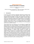
The structure of the muscle model
Sensorimotor
control
Muscle
morphometry
Muscle
mec hani cs
Muscle model
Skeletal
dynamics
Our muscle modeling system is intended for use in a hierarchical framework. The mechanical
dynamics of the skeletal segments comprise the lowest level, and are acted on by a realistic
representation of physiological muscle properties at the middle level. At the top level, the
muscles are controlled by any arbitrary set of activation commands, ranging from pre-recorded
EMG data to dynamic, feedback driven reflex models, to high level simulations of cortical
commands. Our software provides the middle level of the hierarchy. It enables users who may
have only minimal interest in the details of muscle physiology to create realistic mathematical
representations of muscles. At the same time, it is possible for those who wish to delve into and
modify the mathematics of the muscle model to do so. The hierarchical database structure
described below was designed to facilitate such modifications.
1) Fiber type specific det ails
3
2) Whole muscle details, i ncluding
motor uni ts, tendon and
overall morphometry
3) J oint level, with multiple muscles
acting simultaneously
1
2
Fiber type level
It has been shown that the behavior of the contractile element of the muscle scales well from the
sarcomere level up to the whole muscle fiber level and again up to the level of an entire
recruitment group of motor units (Zajac, 1989). There are two critical assumptions behind
“lumping” of individual sarcomeres into a single group:
•
All the sarcomeres in such a group must operate homogeneously, with similar activation,
length and velocity. While some phenomena are believed to arise specifically because of
intra- fiber sarcomere heterogeneity and/or damage (e.g. persistent stretch- induced force
changes), these changes are small or rare under physiological use conditions (Brown and
Loeb, Ms. III).
02/23/ 01
User’s Manual - Virtual Muscle 3.1.5 Documentation.doc
Page 11
•
The sarcomeres must all have the same contractile properties, i.e. their force- length- velocity
relationship, parallel elasticity, and so forth. These characteristics have been shown to be
homogenous within a single histochemical fiber type.
By defining the properties of each fiber type that will be used throughout the model in a single
database, the muscle model can reference these properties when these fiber types are later
combined into typical mixed-fiber-type muscles. The creation of the fiber type database is
handled in a MATLAB function called BuildFiberTypes, which is a graphical user interface
(GUI) described below.
Whole muscle level
Muscles are organized into motor units, each of which consists of a motoneuron and the several
hundred muscle fibers that it controls. All fibers in a unit are the same type. Groups of similar
motor unit types tend to be recruited together. Different types of motor units tend to be recruited
in a fixed order. This fact provides an ideal way to simplify the model. Each whole muscle is
broken into motor units consisting of a single fiber type, with each unit being defined by its fiber
type, its order of recruitment and its force-producing capacity (which is proportional to its total
physiological cross-sectional area). It is assumed that the motor nucleus of the who le muscle
receives a single, time- varying neural activation command signal, which is the apportioned by
the model to activate each unit in turn, according to its defined recruitment order. Within each
motor unit, the frequency of motoneuronal firing is modulated in a realistic manner.
Normally a muscle has about 100 or more motor units. While it is possible to create such a
detailed muscle model with our software, this resolution will make the model run very slowly
and is not usually necessary. For most uses, it will be sufficient to create a small number of
model motor units (perhaps 3-5 for each fiber type), where each unit represents a group of “real”
motor units with a total physiological cross-sectional area (PCSA) of around 10% of the muscle
(first recruited units should be smaller than later recruited ones, as in real muscle). This will
generally produce an acceptably smooth force modulation because of two features built into the
model:
1. The model motor units always produce a smooth output force even at sub-tetanic
frequencies, simulating the force that would have been produced by a large number of
asynchronously active motor units all firing at the same sub-tetanic frequency.
2. The normal range of frequency modulation results in about a 4:1 range of force
modulation, so the force step contributed by a newly recruited motor unit is relatively low
until it gradually increases its firing frequency as activation of the muscle increases
further.
If a muscle is compartmentalized in its mechanical actions and /or different neural activation is
desired for each compartment, each such compartment should be treated as a separate muscle
within the model. For simplicity throughout this document, the term muscle will be used to
denote a single neuromuscular entity with a unidimensional command signal and a homogeneous
mechanical action.
02/23/ 01
User’s Manual - Virtual Muscle 3.1.5 Documentation.doc
Page 12
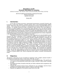
Modified Hill-type model
contractile element
musc le mas s
active contractile
series elastic
element
p aral le l vis co -elastic
motor uni t 1
motor unit 2
motor uni t 3
A given muscle consists of three interacting elements: the contractile element, a series elastic
element, and a muscle mass. The contractile element and series elastic element both act on the
muscle mass, which has inertial properties to prevent instabilities from arising within the muscle.
The contractile element, in effect, consists of as many smaller contractile elements as are defined
by the number of motor units, each of which has a passive parallel elastic element, an
individually defined firing frequency, and force- length- velocity relationships as determined by
the fiber type properties. The parallel elastic element includes a small viscosity for the purposes
of stability. These active sub-compartments sum together to produce the total contractile element
force. Muscles are created using a GUI designed in MATLAB called BuildMuscles which
outputs those muscles as SIMULINK blocks as described below.
Interactions with Neural and Skeletal Elements
Each SIMULINK block representing a muscle must be joined to an appropriate model of the
segment dynamics, which is not provided here. The interaction between the muscle model and
dynamics model is two-way. The muscle blocks produce output force, which is used by the
dynamics model to produce changes in kinematics. These kinematic changes are then passed
back to the muscle model as changes in muscle length, which in turn result in changes in muscle
force. Concurrent with this data exchange must be a source of neural activation for the muscles.
This presumably will arise either from a data file of pre-recorded or pre-generated activations,
possibly from EMG data, or from a control model built in SIMULINK or MATLAB that will
generate the activation for each muscle. As discussed later, it may be necessary or appropriate to
create a nonlinear scaling function between the source data and the activation applied to the
model (see Appendix C).
The dynamics model can be created either within MATLAB or SIMULINK, or it can be linked
to an external application via MATLAB’s DDE interface. A sample implementation of this
function between MATLAB and the WORKING MODEL 2D package is described later in this
document WORKING MODEL.
02/23/ 01
User’s Manual - Virtual Muscle 3.1.5 Documentation.doc
Page 13
Creating the muscle model
Overview
Muscle Morphometry
Fiber_Type_Descripto r
(MATLAB function)
1
S
FR
F
F
her
ot
2
her
ot
4
3
Save
0
Refers to:
Load
Fiber_ Type_Database
(MATLAB .mat data file)
Muscle_M odel_Descriptor
(MATLAB function)
Create as
SIMULINK
blocks
m uscl e 1
m uscl e 2
m uscl e 3
6
Sensorimotor
control
muscle_1.mdl
(SIMULINK block )
musc le_2.mdl
(SIMULINK block)
Musc le
mechanics
m uscl e 4
idual
2
m uscl e 5
ndiv
Type
ort I
5 ve
I mFiber
p
Sa
et d
or
Load
Skeletal
dynamics
0
mi p
1
Musc_Morph_Database
(MATLAB .mat data file)
Existing_Datab ase
(MATLAB .mat data file)
This software package provides a means to simulate the middle layer of the hierarchical model;
that is, the muscle structure and the underlying mechanical function. The steps to use this
software are relatively straightforward.
1. Use the BuildFiberTypes function to define the necessary muscle fiber types in MATLAB.
This function is a GUI that allows the user to define fiber types either from scratch, or to
import existing fiber types from file.
2. Once all fiber types to be used in a given muscle model are defined, they are saved to a
Fiber_Type_Database file. This database can be loaded and edited again, or can have its
fiber types imported into other databases.
3. Use BuildMuscles function to specify a set of muscles composed of varying proportions of
the fiber types defined in steps 1) and 2).
4. Once the desired muscles have been defined they may be saved as a
Muscle_Model_Database file. As before, this file can be opened and edited later.
5. Create muscle SIMULINK blocks using the Create function in the BuildMuscles.
Subsequent changes to an existing simulation can be effected by the Rebuild function, which
searches for and replaces all muscle blocks in a SIMULINK model file with blocks using
updated parameters.
02/23/ 01
User’s Manual - Virtual Muscle 3.1.5 Documentation.doc
Page 14
The BuildFiberTypes function
This function allows the user to create and modify the Fiber_Type_Database.mat files required
for the BuildMuscles function within a GUI. Fiber types may be imported from existing
databases and modified or created entirely from scratch.
Starting up the function
This function is called within MATLAB, so the first step is to run the MATLAB program. The
2
BuildFiberTypes function is invoked by typing :
>> BuildFiberTypes
Creating and editing fiber types in the main descriptor window
2
You must ensure that the BuildFiberTypes.m file is in your current working directory or is in
a directory that is part of your path (the list of directories that MATLAB automatically searches
for files). You can do the former by using dir to obtain a list of the files in your working
directory, and cd to change your working directory at the >> MATLAB prompt. You can check
which directories are part of your path with MATLAB’s path command.
02/23/ 01
User’s Manual - Virtual Muscle 3.1.5 Documentation.doc
Page 15
The main descriptor window allows you to load, save and import from database files, as well as
edit the general parameters for each fiber type. The fiber types are arranged into columns, with
up to five types being displayed on screen at once. If more than five types are created, the user
can scroll to next and previous groups of five fibers using the
or
button.
Editing fiber types
The main descriptor window allows the user to define optimal sarcomere length for the database
(i.e. we force all fiber types in a single database to have the same optimal sarcomere length). If
this value is changed, the user will be prompted as to whether or not they would like the active
and passive force- length relationships scaled appropriately with changing optimal sarcomere
length (the assumption is that the thick filament length stays constant).
In addition, the main descriptor window allows the user to define the following general
parameters for the fiber type:
• Fiber type name: Each fiber type must be given a unique name. Other functions will search
the names in the database for a space and case sensitive match, so consistent naming is
important. If this field is left blank, then no data from this column will be retained when the
database is saved to disk.
• Recruitment rank: The values in this row determine the order in which the fiber types are
recruited within a given muscle. Any numerical value is acceptable, including non- integers.
Those with lowest rank are recruited first; only when all the fibers of this rank are recruited
are the types with the next higher rank recruited. The absolute values of the recruitment ranks
have an effect on the algorithm for automatic apportioning PCSA among simulated motor
units of different fiber types, as discussed below. For most simulations, small integer values
for recruitment rank will work best (e.g. S=1, FR=2, FF=4).
• V0.5 (L0 /s): This is the shortening velocity velocity necessary to reduce force to 0.5 F0 during
a maximal, tetanic contraction. This value is initially calculated from the detailed FV
coefficients, however, changing this value will automatically rescale the related FV
coefficients in the muscle coefficients level. The terms that are specifically affected are bV
and Vmax. As an option, if you change V0.5, you will be prompted as to whether or not you
wish to also scale f0.5 (and related rise and fall time constants) in proportion, because in
normal muscles these values appear to scale proportionally to each other.
• f0.5 (pps): The frequency in pulses per second at which the fibers in the compartment produce
half of maximal isometric tetanic force at 1.0 L0 (see Brown et al., 1999). Similar to V0.5 field
described above, you will be prompted as to whether or not to allow automatic rescaling of
any related coefficients for rise and fall times (see Brown and Loeb, MS IV) and also if you
wish to scale V0.5 in proportion. Again, the default is to allow automatic rescaling. The terms
specifically affected are Tf1, Tf2, Tf3, and Tf4.
• fmin (f0.5 ): The minimal frequency at which a given recruitment compartment is activated
upon threshold activation, relative to the f0.5 frequency. A default value of 0.5 is provided.
• fmax (f0.5 ): The maximal frequency at which a given recruitment compartment is activated
upon maximal activation, relative to the f0.5 frequency. A default value of 2 is provided.
• Comments: Entry into this field is optional. It is a user field that can contain any information
the user desires.
02/23/ 01
User’s Manual - Virtual Muscle 3.1.5 Documentation.doc
Page 16
Underneath these parameters for each fiber type there is a “hidden layer” of fiber coefficients
(see below).
Loading and saving your database
The Save Database and Open Database options under the File menu item allow you to store
the contents of your Fiber_Type_Database at any time, and then reload them for further editing.
Both bring up a standard dialog that prompts you to select a filename to load or save. Files can
have any name, with any number of characters. The name of the database you have saved or
loaded will be reflected in the title bar of the main descriptor window. The only caveat is that
MATLAB may have difficulty identifying files which are not saved with a .mat extension, so
this is automatically appended on to the save filename. It is recommended that you leave this
extension intact so that the save file is easily loaded during future use.
Just before saving, the program will ensure that you have assigned unique fiber names to each of
the fiber types, and prompt you if this has been done incorrectly.
Creating fiber types in your own Fiber_Type_Database file
There are several methods that you can typically use when creating a Fiber_Type_Database file
for your own use.
1) The first method is to open the BuildFiberTypes function and type in all the parameters and
coefficients for each fiber that you wish to use. However, as there are thirty coefficients for each
fiber type, this method is both tedious and prone to data entry errors. Most users will wish to
avoid building their fiber types this way.
2) Another method is to start with an existing Fiber_Type_Database, such as the included
database containing fe line fiber properties, make whatever minor changes are desired to the
existing fiber types, and then save it under a new file name.
3) If you wish to use more fiber types than are provided in an existing database, you may wish to
add new fibers based on other fibers already in the database. This can be done by selecting the
Copy or Cut items from the Edit menu. Either action will open a dialog thatlists the names of the
fibers in the current database. Selecting a fiber type will put the fiber type along with its
parameters and coefficients into the clipboard, which will be reflected in the Clipboard
contains: text string near the top of the window. Note that the Cut option will delete the
selected fiber subsequent to storing it in the clipboard. At this point, selecting the Paste
command will copy whatever fiber type is in the clipboard into the target column. You will be
prompted for a column number to copy the clipboard fiber type in to. The Paste function will
overwrite any contents in the destination fiber type. Note that the clipboard is not a standard
Windows clipboard; thus, fiber type data can not be pasted into other Windows applications
using this function. Note also that the copy, cut and paste operations include both the visible
parameters and the hidden coefficients for a given fiber type.
4) Should you wish to combine fiber types from more than one Fiber_Type_Database, you can
start with an existing database and use the Import action from the Edit menu. This will bring up
a standard file selector dialog. From here, you should select the name of the database that you
wish to import a fiber type from. Next, a list of fiber types in that file will be presented, allowing
you to copy one of those fiber types into the clipboard. The fiber can then be pasted into your
current database.
02/23/ 01
User’s Manual - Virtual Muscle 3.1.5 Documentation.doc
Page 17
Editing fiber coefficients
For most purposes, users should be able to obtain a reasonable approximation of the function of
most mammalian muscle fiber types by modifying the V 0.5 and f0.5 properties of the fiber types
imported from the two databases we provide, and allowing the BuildFiberTypes function to
rescale any related coefficients.
However, should you wish to access the details of each equation at a lower level, selecting the
Edit Coefficients item from the Fibers menu will bring up the fiber specifics window,
allowing modification of any of these coefficients. The equations related to these coefficients are
available in Appendix B of this document (see Brown et al., 1999, Brown and Loeb, 2000 and
Cheng et al., 2000 for a detailed description of these coefficients).
Clicking the
or
buttons will allow you to modify the coefficients for the
previous or next fibers respectively. To return to the main window, click on the
button.
Editing generic coefficients
Specific tension, tendon properties and passive force properties (including viscosity) have their
own sub- menu in the BuildFiberTypes function.. These properties are assumed to be constant
for all fiber types in a given database.
Help
Selecting the Help menu item will bring up a window describing the definition of each property
listed in the current window. For a more detailed explanation of the equations and their related
coefficients used in the muscle model, please see Brown et al. (1999), Brown and Loeb (2000),
Cheng et al. (2000) or see Appendix B.
02/23/ 01
User’s Manual - Virtual Muscle 3.1.5 Documentation.doc
Page 18
The BuildMuscles function
Once a Fiber_Type_Database.mat file has been created, these fiber types can be combined in
varying proportions to produce SIMULINK blocks that model muscle force output, complete
with sequentially recruited motor units of varying size and fiber type, and intra-muscle
interactions between active contractile elements and parallel and series elastic elements.
The function allows muscle data to be stored in two representations. The first is as a
Muscle_Database.mat data file in MATLAB. This stores the current configuration of each
muscle and can be loaded into the BuildMuscles function to be edited again. This database file
is only used by this function and will not constitute part of your simulation. In order to use the
muscles, you must generate the second representation as a SIMULINK block.
Starting up the function
From within MATLAB, this function is invoked by typing 3 :
>> BuildMuscles
Creating a new muscle model database
If you wish to create a new muscle model database, you should select a
Fiber_Type_Database.mat file to use, from the Select Fiber Type Database item from the
File menu. If you have not yet created one, return to the previous section and create one using
the BuildFiberTypes function. The Fiber_Type_Database.mat file selected at this point is
permanently associated with the created muscle database, and any changes made to the fiber type
database will be reflected in the muscle model, so long as the fiber type names remain consistent.
Once a Fiber_Type_Database file has been selected, or an existing Muscle_Database has been
loaded, the name of the associated fiber type database file will be reflected in the Fiber Type
Database: text string near the top of the window.
It is possible to change the Fiber_Type_Database.mat file associated with a Muscle_Database
by choosing the Select Fiber Type Database option when a muscle model database is already
open. The limitation is if existing fiber types present in the original muscle model database are
not present in the new fiber type database, there must be enough new or unused fiber types that
can replace the old ones, else an error will occur.
It is not recommended that you keep multiple copies of a single Fiber_Type_Database in
different directories of the MATLAB path, as this will make it difficult to track which file is
being used at any given time.
3
As with the BuildFiberTypes function, the BuildMuscles.m file must be either in the current
directory or in the MATLAB path.
02/23/ 01
User’s Manual - Virtual Muscle 3.1.5 Documentation.doc
Page 19
Editing muscle types in the main descriptor window
The main descriptor window allows users to load, save, and edit a Muscle_Database, each of
which is constructed of a combination of fiber types as described in the fiber type database. Each
muscle from the database can be created as a SIMULINK block for use in a biomechanical
model.
Loading and saving
If you choose to Load an existing database from the File menu, a dialog will open asking for the
name of the existing database file. Note that the Fiber_Type_Database.mat file you used in the
creation of this muscle database must either be in the current directory or in the MATLAB path.
If the expected Fiber_Type_Database.mat file cannot be found, you will be prompted to select
one. This database must contain at least as many fiber types as are used by the muscle database.
The program will prompt you to choose which fiber types to associate with which if the names
do not match. Ensure that a valid database file has been loaded before proceeding to edit your
muscles or errors will result.
The Save item in the File menu allows you to store your muscle parameters for later
modification. It is recommended that muscle model files be saved using a .mat extension.
Copying, cutting and pasting muscles
It is possible to Copy, Cut, and Paste muscles to and from the clipboard using the items from the
Edit menu. Contents of the clipboard will be reflected in the Clipboard contents: string at
near the top of the window.
02/23/ 01
User’s Manual - Virtual Muscle 3.1.5 Documentation.doc
Page 20
Importing muscles from another database
As with fiber types, muscles can also be imported from other Muscle_Database.mat files.
Selecting Import muscle from the Muscles menu will open a file selection dialog, allowing you
to select another muscle model database file, and select a muscle from that file. This muscle data
will then be stored in the clipboard for pasting into the currently open database.
Editing muscles
The main descriptor window allows ten rows of muscles to be viewed and edited simultaneously.
Scrolling through muscles if more than five are used is accomplished with the
and
buttons. The muscle parameters that may be modified are:
• Muscle name: A unique name for each muscle must be input here. Muscle data for each row
will be saved to the database file only if a name is entered.
• Muscle mass (g): Mass of the muscle belly in grams.
• Fascicle L0 (cm): Average length of the fascicles in the muscle belly, when the muscle is at
its optimal length for production of isometric tetanic force (note that this value is typically
10-30% less than the length at which optimal twitch force is generated, Close, 1972; Roszek
et al., 1994; Brown and Loeb, 1998).
• Muscle PCSA (cm2 ): Physiological cross-sectional area of the muscle. This value cannot be
input directly, and is instead calculated from values input for muscle mass and fascicle
length. A muscle density of 1.06 g/cm3 is assumed (Mendez and Keys, 1960).
• Muscle F0 (N): The maximal amount of force that the muscle can produce isometrically.
This value cannot be entered directly, and is calculated from the muscle PCSA, multiplied by
a standard value for specific tension of muscle. The default specific tension for mammalian
muscle (defaults to 31.8 N/cm2 , Brown et al., 1996) can be modified by selecting the Change
specific tension item from the Muscles menu.
• Tendon L0 T (cm): Length of the tendon at the muscle’s optimal force. This term should
consist of the total amount of connective tissue in series with the muscle fascicles, including
both internal aponeurosis and external tendon. This value must be greater than zero; this
value will default to 0.1 cm if no value is entered. The coefficients for the properties of the
tendon can be modified from their defaults with the Edit tendon properties item from
the Muscles menu. The tendon is modeled on a log/linear relationship (Brown et al., 1996).
L0 T is the length of the tendon when stretched with force F0 ; this is well up in the linear
stiffness range. As the tendon shortens by 3.6% from length L0 T , force drops linearly to
about 20% of F0 , followed by an exponential decrease to slack (essentially zero tension) at
95% of L0 T . While the total range of length of tendon is small, it can exert large effects on
muscle force because it changes the way in which velocity of the whole- muscle length
appears at the contractile elements, which are very velocity-sensitive. This is particularly
true in muscles that have substantially longer tendon+aponeurosis than fascicle length.
• Max. whole-muscle length (cm): Maximum length of the whole- muscle (entire
musculotendon path length) at the most extreme anatomical position. This value is used to
calculate the following Lmax parameter, which controls passive tension.
• Fascicle Lmax (L0 ): The maximal length of the fascicles at extreme anatomical position of the
skeleton, measured in terms of the optimal fascicle length. This value cannot be entered
directly, and is calculated from the difference of the Max. whole- muscle length and the
02/23/ 01
User’s Manual - Virtual Muscle 3.1.5 Documentation.doc
Page 21
•
•
Tendon L0 T , scaled by fascicle L0 . Reasonable values of Lmax are typically greater than 1, but
less than 1.3.
Ur: Fractional activation level at which all motor units for a given muscle are recruited (i.e. it
is the threshold of the last motor unit) for the ‘Natural’ Recruitment algorithm provided
Once activation has reached Ur, further increases in activation result only in frequency
modulation up to fmax for each motor unit at U=1. A reasonable default value of 0.8 is
provided. Lower value s are more appropriate for muscles with unusually homogenous fiber
type composition.
Fiber type distribution (PCSA/# of motor units): The fraction of total muscle PCSA and
the number of motor units assigned to each fiber type. The fiber types named at the top are
determined by those present in the selected Fiber_Type_Database. The two values are
separated by a forward-slash (/) for each fiber type. Note that the PCSA assigned to the fiber
types for each muscle must total 1.0, otherwise an error will be reported when attempting to
save your database. Should this occur, you will be presented with an opportunity to either 1)
have the BuildMuscles function automatically redistribute the PCSA among the fiber types
in the same proportions, but such that they total 1.0, 2) to save the muscle with the incorrect
PCSA total, or 3) to cancel the save and manually redistribute the PCSA. Scrolling through
more than the five visible fiber types is accomplished by clicking the
or
buttons near the top of the window. In the example of Figure 7, Muscle #1
(Brachialis) is composed of 50% S type fibers, and 50% FF type fibers, with the names being
taken from the fiber type database the user has loaded. Of these fiber types, 2 motor units are
allocated to the S fibers and 3 to the FF fibers.
Size of motor units
Each real motor unit innervates a fraction of the muscle’s total PCSA. Realistic recruitment of
biological motor units during activation occurs in a fixed sequence, with smaller and slower
motor units being recruited first according to Henneman’s size principle. For example, motor
units innervating slow-twitch muscle fibers are typically smallest, while motor units for the
larger fast-twitch fibers are recruited later. To reproduce this orderly recruitment based on fiber
type, the Recruitment_Rank parameter in the BuildFiberTypes function determines the order
of recruitment of motor units composed of different fiber types, if the ‘Natural’ recruitment
strategy is selected (as described below) .
Within motor units of the same muscle fiber type, Henneman’s size principle still applies in real
biology; for example, motor units that innervate a smaller number slow-twitch fibers will tend to
be recruited before motor units that innervate a larger number of slow-twitch fibers. However, in
the muscle model motor units within a fiber type are recruited in the order in which they are
listed (e.g., Unit #1, Unit #2, Unit #3, etc.) and PCSA is assigned to each motor unit
individually. So to maintain Hennemann’s size principle in a model, motor units should be listed
in order of size (smallest to largest), at least for ‘Natural’ recruitment strategies.
In a perfect muscle model, each motor unit would be represented individually, and thus each
slow-twitch motor unit would have a smaller PCSA assigned to it than a fast-twitch motor unit.
This would make the computations unnecessarily lengthy, however. The model allows the
number of simulated motor units (and hence resolution of the simulation) to be specified by the
user. It then apportions the PCSA of the muscle among those units according to one of several
02/23/ 01
User’s Manual - Virtual Muscle 3.1.5 Documentation.doc
Page 22
algorithms. In a typical simulation with 10 motor units, each motor unit would actually reflect
the contribution of about 10 “real” motor units.
The allocation of the total PCSA of the muscle to each simulated motor unit can be viewed and
edited by choosing the Manually distribute unit PCSAs item from the Muscles menu. A
dialog will allow you to select the muscle to modify. A muscle specific window will open, listing
the proportion of the muscle’s PCSA that is apportioned to each motor unit and each different
fiber type.
By default, assigning PCSA and number of motor units to a previously unassigned fiber type
(i.e., with a previous PCSA/# motor units of 0/0) will result in an automatic distribution of PCSA
for the motor units of that muscle and fiber type using the ‘default’ apportioning algorithm. For
the ‘default’ apportioning scheme, the proportion of PCSA automatically allocated to each motor
unit is based on the Recruitment_Rank parameter for the fiber type and on the total number of
units of that type; as in the following equation:
PCSA
n th motor unit
= PCSA assignedto fiber type ×
Recruitment_Rank + n
(Recruit_Ra nk + 1) + (Recruit_Rank + 2) + ... + (Recruit_Rank + total# motor units)
Effectively, this distribution scheme assigns a larger proportion of PCSA to later recruited motor
units of a given type. Increasing the absolute value of the Recruitment_Rank parameter for the
fiber type reduces the differences in PCSA between consecutively recruited motor units. Because
the Recruitment_Rank values of late recruited fiber types must always be greater than those of
early recruited types, the distribution will always represent the physiological phenomenon
whereby fast- fatigable units (which have a higher Recruitment_Rank ) have a smaller range of
sizes than slow-twitch units (Burke et al., 1973). Note that if you change the Recruitment_Rank
parameter to change the automatic redistribution properties, you must ensure that the
Recruitment_Rank for all other fiber types still accurately reflects the order of their recruitment.
If a user wishes, he/she can manually enter in the PCSA of each motor unit to override the
automatic distribution.
The user can also choose one of two other automatic apportioning schemes, each of which can be
applied to either a single muscle or multiple muscles. The ‘geometric’ one will ask the user for
the fractional increase between one motor unit and the next, and will then distribute the PCSAs
appropriately for each fiber type. The ‘equal’ one simply makes all motor units of each fiber
type equal in size to the other motor units of that fiber type.
02/23/ 01
User’s Manual - Virtual Muscle 3.1.5 Documentation.doc
Page 23
The above figure depicts the automatic (‘default’) distribution of the PCSA in Muscle #1
(Brachialis) using 50% Type S in 2 motor units and 50% type FF in 3 groups. Thus, the two S
units were sized to 21.4% and 28.6% of the total PCSA each, and the three FR units were sized
to between 13.3% and 20% each. Note that consecutive FF motor units have a smaller change in
proportion of PCSA, because FF fibers have a higher Recruitment_Rank. This model would be
more realistic, particularly at low recruitment levels, if the relatively large fraction of total PCSA
occupied by S units were divided into a larger number of smaller units such that the largest S unit
was smaller than the smallest FF unit. The sudden recruitment of a relatively large unit at the
beginning of muscle activation will create an unphysiologically large step in force (although the
problem is not as severe as might be thought because of the ongoing frequency modulation of the
units after their initial recruitment).
These numbers can be manually edited by typing new values into each field. If you change the
total PCSA allotted to a fiber type, the individual unit PCSAs will be updated using the
Apportioning method for that fiber type. If one of the unit PCSAs is manually updated, then the
total PCSA for that unit will be updated automatically, and the apportioning method for that
fibertype will change to ‘manual’. Different apportioning methods can be chosen by chosen
under the Muscles menu.
If there are more than ten motor units of a given fiber type, the
and
can
be used to scroll through them. If more than five fiber types are used, the
or
buttons are used. When changes are completed, select the Close option from the
File menu.
Recruitment of motor units
Currently, two different recruitment strategies can be chosen from: ‘Natural’ and ‘Intramuscular
FES’. Each one results in the creation of a SIMULINK block within the muscle block that takes
the appropriate activation input and divides it into the recruitment and frequency outputs for each
motor unit. For ‘Natural’ recruitment the activation input is assumed to be the relative strength
02/23/ 01
User’s Manual - Virtual Muscle 3.1.5 Documentation.doc
Page 24
of the net synaptic drive or EMG envelope. The ‘Natural’ recruitment strategy recruits all motor
units of a lower Recruitment_Ranked fiber type before recruiting any motor units of the next
highest Recruitment_Ranked fiber type. Within each fiber type, motor units are recruited in the
order in which they were listed (i.e. it assumes that the motor units were listed in order of size).
The frequency of each unit begins at fmin when that unit is first recruited and reaches a maximum
of fmax when input activation equals 1.
The ‘Intramuscular FES’ strategy requires both an activation and a frequency input. The
frequency input is assumed to be the frequency of stimulation being applied to the muscles and is
the same (in units of pps) for all motor units. The activation is the relative strength of the
stimulus. Motor units within each fiber type are recruited in the order in which they were listed,
however, no distinction is made between recruitment rank. Instead the motor units are recruited
so as to equalize the fraction of each fiber type recruited. A linear relationship between the
fractional PCSA recruited and activation is maintained.
Additional Outputs
There is an option to add one or more of several outputs to each SIMULINK block, in addition to
the force (N) output. These have been added because some of them may be necessary to provide
as feedback to a neural circuit. The current choices are: activation, fascicle length (L0 ), fascicle
velocity (L0 /s) and Force (F0 ).
Creating a SIMULINK block of one muscle
Once all details have been finalized to your satisfaction, a SIMULINK block which has been
assigned the name of your muscle can then be created by selecting the Create SIMULINK
Muscle Block item from the Model menu. This will launch SIMULINK and create a block that
can be drag-and-dropped into your working SIMULINK figure. A SIMULINK block can be
created as many times as desired, and for as many different defined muscles as desired. If you
wish to utilize the Rebuild Existing SIMULINK Model function described below, it is
necessary that the SIMULINK block name be kept the same. The use of these blocks is
explained in the subsequent section.
Rebuilding an existing SIMULINK model
After you have used the SIMULINK muscle blocks in a model, you may wish to modify the
parameters for each muscle or for the fiber types comprising the muscle blocks. The Rebuild
existing SIMULINK model option from the Model menu allows you to select an existing
SIMULINK model and will replace each muscle block in that model. This function works by
searching the SIMULINK model for any blocks with names that match the muscle names in the
currently open Muscle_Database. Any blocks with matching names will be replaced with a
newly created SIMULINK block of that muscle, using the current parameters in the muscle
model database and its associated fiber type database.
This facility allows you to easily modify the parameters for your muscles and test the effects of
their changes on your simulation.
02/23/ 01
User’s Manual - Virtual Muscle 3.1.5 Documentation.doc
Page 25
Using the muscle model
Structure of the SIMULINK block
Once you have created your Muscle_Database, you can create blocks of physiologically
functioning muscle from the BuildMuscles function. The SIMULINK blocks are based on a
modified Hill-type muscle model, which is described in detail in Brown et al. 1996. Although it
is not necessary to understand the internal details of the muscle block, they are summarized here
briefly. If you are not interested in the internal details, proceed to the next section.
In summary, each SIMULINK muscle block contains a contractile element (which is composed
of an active element and a parallel visco-elastic element) and a series elastic element. For
modeling purposes, a muscle mass is interposed between the contractile and series elastic
elements to prevent unrealistically large, instantaneous accelerations and instabilities that occur
if the velocity dependent contractile element is connected directly to the series elastic element.
Descriptions of SIMULINK subsystems used to model each of the elements are given below:
• Recruitment block: This element represents the motor pool (for natural recruitment) or
stimulators (for FES). A single activation input (plus a frequency input for FES) is
transformed into frequency outputs for each motor unit of that muscle. The combined vector
is sent to the CE + PE element to calculate active force.
• Contractile element + Passive element subsystem: This element represents the fascicles in
the muscle belly. Its output, force, is determined by three inputs; activation, fascicle length
and fascicle velocity. Note that the fascicle length input to this subsystem is different from
the entire musculotendon path length value which is input to the whole- muscle block. It is
assumed that pennation angle is negligible for this model. Fascicle velocity is computed
within the SIMULINK block by integrating the calculated acceleration. Also note that this
element calculate the active and passive forces for the fascicles.
The block representing the contractile element subsystem consists of one sub-block for each
fiber-type within that muscle. Each of those fiber-type specific blocks then contains blocks
that calculate those muscle properties which are the same for all motor units (of that fibertype) as well as one sub-block for each motor unit as defined in the BuildMuscles function.
The force blocks for each motor unit sum together to produce a force output for each fiber
type block, which then sum to produce a single force output for the entire contractile
element.
• Series elastic element subsystem: This element represents the effective length of the
internal and external tendons; aponeurosis elements should be included. The force produced
by this element is dependent only on length, and has been shown to have no significant
velocity dependence at physiologically relevant frequencies. For this reason, changes in the
musculotendon path length are made to act directly on the series elastic element.
A single function block provides all the calculations for this element. Note that the length of
this element is calculated by subtracting the length of the contractile element from the
musculotendon path length.
• Muscle mass subsystem: The muscle mass was included to prevent the system from
becoming unstable as the series elastic element and contractile element act on each other.
02/23/ 01
User’s Manual - Virtual Muscle 3.1.5 Documentation.doc
Page 26
Position of the muscle mass within the block is tracked by first converting the force produced
by the contractile and series elastic elements into a net acceleration, based on the size of the
mass. Acceleration is then integrated to give a velocity, and integrated again to give the
position of the mass. Velocity and position of the mass are fed back into the contractile
element, and position is subtracted from the musculotendon length and fed back into the
series elastic element.
m us c le_1. mdl
( S IMULI NK bl ock )
SIM ULIN K i mplementa ti on
Modified Hill -type model
co ntr act ile e le m en t
m uscle m as s
active contractile
series elastic
e le m ent
parallel visco-elastic
mo t or unit 1
mo to r u nit 2
mo t or unit 3
Using the muscle blocks
Each SIMULINK whole- muscle block has at least two inputs and at least one output. A few
common implementations are briefly discussed, but these will vary based on the form of the
segment and activation data provided in your simulation. The two required inputs are:
• Length: The musculotendon path length is required in units of cm. Note that this value may
have to be calculated from the available data in the skeletal dynamics model, as often only
segment coordinates or joint angles are provided.
• Neural activation: This is a value for activation of the active part of the contractile element.
This value is clipped between 0 and 1. The recruitment element of the muscle converts this
activation (and possibly using other inputs, e.g. frequency for the case of FES recruitment)
into an effective firing frequency of the motor units of the muscle. Typical inputs for
‘natural’ recruitment might be from EMG data scaled to the level of maximal voluntary
contraction, or a simulated α-motoneuron that is controlled by reflex feedback or a neural
network.
02/23/ 01
User’s Manual - Virtual Muscle 3.1.5 Documentation.doc
Page 27
•
Frequency: This value is only required for FES recruitment and is the stimulus frequency
(pps) being applied to the motor pool.
A single required output is provided from the SIMULINK block:
• Force (N): The force is measured at the series elastic element. If the muscle is to act at a
joint to create a torque, it is important that the moment arm which the muscle acts through is
realistic.
The force produced by the muscle is positive in sign. Thus, the output may have to be
multiplied by –1 depending on the implementation of the skeletal mechanics portion of your
model.
• Force (F0 ), Activation, Fascicle Length (L0 ) and Fascicle Velocity (L0 /s): These outputs
are optional, and may be of use when providing feedback to a controller. The activation is
just a wire through of the activation input. Force, Length and Velocity are simply the
normalized versions of these variables.
Interacting with models of segment dynamics
As discussed previously, a model of the segment dynamics is not included, as this model was
intended to provide only realistic muscle forces, and the segment systems are typically so
specific that a generic model would not be useful for most users. This muscle model fits best
with systems that have been designed hierarchically; i.e., that have existing handles for muscles
that would allow forces to act directly on segments. Especially with SIMULINK based models,
incorporating this muscle model would be trivial, as the force outputs from the desired muscles
could easily be summed, modified by any requisite moment arm or other scalars and connected
to the segment dynamics model.
Model integration will work well with any hierarchically designed models in other packages that
can interface with MATLAB (an example being WORKING MODEL 2D; a sample
implementation using dynamic data exchange [DDE] is described in the following section).
02/23/ 01
User’s Manual - Virtual Muscle 3.1.5 Documentation.doc
Page 28
Muscle_System.mdl
(SIMULINK system)
u_ 1
In_ 1
u _2
In_2
u_3
Se nsor imotor
control
In_3
u_ 4
In_4
u _5
Mus cle
morp ho metr y
Mu scl e
me chan ics
In_5
m uscle_ 1.m dl
(SIMULINK block)
Out_1
muscl e_2.mdl
(SIMULINK block)
Out_2
muscle _3.m dl
(SIMULINK block)
Out_3
muscle _4.m dl
(SIMULINK block)
Out_4
mu scle_ 5.md l
(SIMULINK block)
Via gl obal
variables
Out_5
Via out ports
Mu sc le mod el
Sk elet al
dyna mi cs
SimDDE.m
(MATLAB function)
DDE Link
DDE Li nk
Any dynamic s modeling
package that supports
DDE
Interacting with a controller model
A control block created within SIMULINK is well suited to providing the activation levels
needed for each muscle block. This controller can easily receive input from the segment
dynamics model to provide feedback control of the muscles. This control can be supplemented
by or replaced with pre- generated muscle activation levels, such as those recorded from EMG
signals. SIMULINK allows simple access to data such as EMG signals recorded over time via
either a From Workspace block or a From File block. Essentially, the data must be in tabular
form with time values as one column, and any other values to be passed into SIMULINK as
other columns. Detailed instructions are given in the SIMULINK documentation.
External software that can exchange data with MATLAB can also be used as the controller
model. In Windows, DDE is a common standard to facilitate inter-software communication. The
SimDDE example given in the following section can be modified to suit this role.
Editing the muscle blocks
Each SIMULINK muscle block contains fixed equations and constants as defined in the original
Fiber_Type_Database.mat and Muscle_Database.mat files at the time of the creation of the
block. Once the muscles have been created and linked into a SIMULINK model, their parameters
can be changed by modifying the information in the original Fiber_Type_Database.mat and
Muscle_Database.mat files and using the Rebuild Existing SIMULINK Model from the
BuildMuscles functions. In this way, it is simple to observe the effects of different muscle and
fiber type parameters on the behavior of your system. As described previously, the names of the
02/23/ 01
User’s Manual - Virtual Muscle 3.1.5 Documentation.doc
Page 29
muscle blocks in your SIMULINK model should match the names of the muscles in your
Muscle_Database.mat file should you wish to use the rebuild function.
To examine the structure of the muscle model, double-click on the whole muscle block. This will
reveal the SIMULINK blocks that make up the muscle model. At this level editing the details
directly is not recommended, but is possible. For conceptualization purposes, the blocks are
loosely grouped into a contractile element subsystem of blocks, a series elastic element
subsystem, and a muscle mass subsystem. The visible lines control the flow of data between the
subsystems.
Running your simulation
The muscle block that you have created behaves like any other standard SIMULINK block.
Inserting it into any existing system or .mdl file will allow you to click on the
icon in
SIMULINK or to use the SIM command from within MATLAB to start your simulation.
Initial conditions for the muscle mass block
At the first time-step of the simulation, positions of all internal muscle masses and hence the
starting lengths of each contractile and elastic element are chosen based on the initial conditions
predefined by the model. The initial fascicle length conditions can be modified within the muscle
mass subsystem by changing the default conditions for the muscle mass position integrator. By
default, the position is set to a position that is almost exactly in equilibrium (if the passive force
of the muscle is less than 5% of maximum, this position will be accurate to better than 0.1%). At
extremely long lengths or if the passive force equations are changed such that there is significant
passive force at the start of a simulation, the system will have to be allowed to reach equilibrium.
After the first time-step, the positions of all the internal muscle masses are stored in a state
vector that is continuously updated by SIMULINK. These state values are important so that
SIMULINK can remember the lengths and velocities of each contractile and elastic element. If
your simulation is run uninterrupted, this state vector is completely transparent to the user and
does not need to be considered. However, if you plan on stopping your simulation and restarting
it at different times, this state vector will have to be stored on stop and reloaded on restart to
avoid going through a new settling period. Doing this may be necessary if you are interfacing
with an external simulation package, such as to model system dynamics. An explanation of this
procedure is given in the following section describing a sample implementation of this model.
Common problems
Using experimental data
One typical use of muscle models is to predict muscle force from experimentally recorded data
for activation and length. Kinematic data often have noise or quantization errors that are
magnified when the length data are differentiated to produce velocities of muscle stretch, as
shown below. Note that while the position signal appears smooth, when differentiated in the
SIMULINK model, the velocity is not smooth. Because muscle fiber velocity has such a large
effect on force output, it is us ually desirable to apply a modest smoothing function to your length
data before sending it to the SIMULINK muscle model block.
02/23/ 01
User’s Manual - Virtual Muscle 3.1.5 Documentation.doc
Page 30
Insufficient accuracy
The tolerances for inaccuracy that SIMULINK uses can be viewed in an open .mdl document
under the Simulation→Parameters→Solver menu. The default relative tolerance for
SIMULINK 3.0 is 1e-3. Any errors in integration detected when the simulation runs above this
value will result in SIMULINK automatically reducing its time step sizes. For most muscle
models, a relative accuracy of 1e-6 is sufficient to prevent instabilities from arising under
physiological conditions. If accuracy conditions are not stringent enough, SIMULINK may not
return any errors, but the force output between time steps may be change drastically, as opposed
to gradually. This may be reflected in the kinematics of the system you are modeling by
instability or jerkiness. Try tightening tolerances by an order of magnitude to see if this resolves
the issue.
An example is depicted below. On the left, a muscle is given a constant level of activation and
has a constant velocity ramp stretch applied, using the default relative accuracy in SIMULINK of
1e-3. Note the spikes in the force trace corresponding to inaccuracies in integration. On the right,
the same conditions but with relative accuracy tolerance tightened to 1e-6. In both cases, for the
first 20 ms, there are initial force transients relating to the “settling” of the contractile element
and the tendon. This is unrelated to the integrator tolerances, and is discussed in a following
section.
02/23/ 01
User’s Manual - Virtual Muscle 3.1.5 Documentation.doc
Page 31
Inappropriate initial conditions
Muscles with a zero tendon length will not function properly. To counteract this, a minimum
tendon length of 0.1 cm is attributed to muscles specified in the BuildMuscles function.
Scaling of activation inputs with multiple motor units
A consequence of simulating multiple motor units is that the recruitment function used in this
model produces a non- linear response in the conversion from input activation into effective
muscle activation such as might be measured by EMG. This arises because increasing activation
linearly increases the frequency envelope of any currently recruited motor units and also recruits
additional motor units. Suggested solutions are described in Appendix C.
Unrealistic simulation conditions
If muscles are stretched to extremely long lengths (i.e., if the contractile element of the muscle
exceeds 1.85 L0 ), SIMULINK will likely return the following warning.
Warning: Attempt to raise negative value to a non-integer power in
'untitled/Brachialis/contractile element/Fiber 1/Af'.
This results from the method used to determine rise and fall times for the effective activation of
the muscle. While exact solutions for Af would not produce these errors, numerical solutions can
be inaccurate. If this warning arises, check the lengths for the muscle indicated by SIMULINK.
Simulation running too slowly
While the use of multiple motor units allows a combination of muscle fiber types and serves to
increase accuracy of muscle force production, an inherent drawback is the increased
computational time required for your simulation. Depending on the level of accuracy desired, the
use of multiple motor units may not be necessary to replicate relatively realistic muscle behavior.
Additionally, for the purposes of familiarizing yourself with the muscle model software and to
first set up your model, it may be desirable to use single motor unit muscles, which can later be
replaced with muscles that have multiple units and fiber types using the Rebuild Existing
Muscle Model option in the BuildMuscles function. To facilitate a simple but effective single
motor unit muscle, you should modify the minimal firing frequency (fmin ) of the fiber type to be
used in your muscle to be zero (in the BuildFiberTypes function), and specify the Ur (in the
BuildMuscles function) for that muscle to be zero.
02/23/ 01
User’s Manual - Virtual Muscle 3.1.5 Documentation.doc
Page 32
Interfacing with non-MATLAB applications
Provisions are provided in many simulation packages for dynamic data exchange (DDE) that
allow MATLAB to control one aspect of the simulation. In this case, it is possible to use
MATLAB’s DDE interface to allow SIMULINK to pass data to and from another application
(SIMULINK cannot do this directly). This can be affected by writing a MATLAB “wrapper”
function that acts as an intermediary between your external application and the SIMULINK
model.
The MATLAB wrapper must call SIMULINK to run over a time-step that matches the time-step
of the external application. Inputs to the MATLAB function will vary depending upon the
specifics of the external application. As mentioned previously, for all time-steps except the first
one, SIMULINK relies on a vector of saved state variables that allow the muscle model to
resume its run with the lengths and velocities of the elements within the muscle being retained.
Data is passed out of the MATLAB wrapper in the form of variables which may be in vector or
scalar form. The way in which your application utilizes these will vary.
A sample implementation of this function is given in the included SimDDE code. This acts to
pass muscle data from SIMULINK into WORKING MODEL 2D software, which provides an
easy-to- use system for modeling segment dynamics.
Muscle_System.mdl
(SIMULINK system)
u_ 1
In_ 1
u _2
In_2
u_3
Se nsor imotor
control
In_3
u_ 4
In_4
u _5
Mus cle
morp ho metr y
Mu scl e
me chan ics
In_5
m uscle_ 1.m dl
(SIMULINK block)
Out_1
muscl e_2.mdl
(SIMULINK block)
Out_2
muscle _3.m dl
(SIMULINK block)
Out_3
muscle _4.m dl
(SIMULINK block)
Out_4
mu scle_ 5.md l
(SIMULINK block)
Via gl obal
variables
Out_5
Via out ports
Mu sc le mod el
Sk elet al
dyna mi cs
SimDDE.m
(MATLAB function)
DDE Link
DDE Li nk
Dyanmic s_Sys tem.wm
(Working Model 2D document)
muscle_1
mus cle_2
muscle_3
mus cle_4
muscle_5
02/23/ 01
User’s Manual - Virtual Muscle 3.1.5 Documentation.doc
Page 33
A sample application using WORKING MODEL 2D
Getting started
The software packages required to run this demonstration are:
• MATLAB 5.2 or higher
• SIMULINK 2.2 or higher
• WORKING MODEL 2D 4.0.1 or higher
The files required for the use of this sample function are:
• SimDDE.m
(MATLAB wrapper function)
• Dynamics_System.wm
(WORKING MODEL 2D simulation template using
SimDDE)
•
Muscle_System.mdl
(SIMULINK muscle block)
The combination of the first three files listed are required to run the SIMULINK driven model.
First, ensure that MATLAB is already open, and that the required files are in the current working
directory or are part of your path. Next, open WORKING MODEL 2D and open the
Dyanmics_System.wm file.
A simple skeletal system in WORKING MODEL 2D
WORKING MODEL 2D provides an easy-to-use graphical interface for building dynamic
systems. It allows the user to specify many important details of a simulation, including contact
forces, gravity, and linkages, without the need to write explicitly the equations of motion.
WORKING MODEL 2D provides useful tutorials and help files and we refer the user to those to
learn how to build a system like the one shown here.
02/23/ 01
User’s Manual - Virtual Muscle 3.1.5 Documentation.doc
Page 34
The Dynamics_System.wm file provides a simple skeletal system with five pre-created muscles
and two skeletal segments. These muscles (or in WORKING MODEL terminology - actuator
elements) are linked to our SIMULINK muscle model ‘engine’ via an application interface.
Because our SIMULINK model represents whole- muscles, the tendons are not explicitly
represented here. When the simulation is running, at each time step, information on the length of
each actuator/muscle is reflected in the meters at the top-left side of the screen. These meters
then pass the information on the actuator length to the application interface, which communicates
this information to MATLAB via DDE. Muscle forces are received from MATLAB and
displayed in the muscle force input boxes on the bottom- left corner of the screen. The length
meters and force inputs are essential to the operation of the link and should not be deleted,
although they may be moved or made invisible.
02/23/ 01
User’s Manual - Virtual Muscle 3.1.5 Documentation.doc
Page 35
Controlling muscle activation
Muscle activation levels are controlled within the SIMULINK layer. The muscles can be
examined by running SIMULINK, and then opening the m5.mdl file. Five muscles will be
displayed, each with two inputs and one output. The elliptical Out ports are the handles through
which information is passed from SIMULINK to MATLAB and then to the DDE. The square
inputs for Activation_1 through Activation_5 are local input values for activation of each
muscle, and should be between 0 and 1. These can be set at fixed levels directly, or replaced with
other SIMULINK blocks to simulate a neural controller mechanism.
Note that lengths are not passed into the SIMULINK model directly via the elliptical In ports
and are instead passed to the MATLAB workspace, and then into SIMULINK via a From
Workspace block. This allows SIMULINK to interpolate lengths between time steps, providing
more accurate velocity effects.
The SimDDE wrapper in MATLAB
The SimDDE.m MATLAB function works simply by telling SIMULINK to run the desired model
at a single time, for the duration of one time-step. If the start time entered is 0, then the wrapper
function assumes that it is the first step and calls the model with the initial conditions for various
lengths and velocities of the elements in each muscle. At the end of each SIMULINK time-step
run, muscle force and other variables are passed out of MATLAB to the DDE. Additionally,
SimDDE saves a state vector of the lengths and velocities of the elements within each muscle
block to a global variable. If the start time entered is greater than 0, then SimDDE will load the
state vector from the global workspace and run the muscle model with these initial conditions.
SimDDE automatically adjusts its time-step to match tha t of the linked application. The global
02/23/ 01
User’s Manual - Virtual Muscle 3.1.5 Documentation.doc
Page 36
variable, called tempStateStorage, is transparent to the user and does not need to be
manipulated in any way.
Users who wish to program their own external application interfaces for this muscle model
software should examine the code for the SimDDE.m function because the specifics of
implementation depend on both the application software and the model being created on it.
Details on the changes necessary are outlined in the comments within the actual code.
Optimizing your simulation
As a first step, once all the desired segments have been created and linked, the simulation should
be run for several frames with zero activation to each muscle to ensure that muscles were
inserted at reasonable lengths. Actuator/muscle elements that are being held at lengths much
greater than optimal will generate large passive forces and will rapidly pull the system away
from its starting position even without activation; this should be checked and accounted for. It
may be useful to adjust slightly the origin and insertion points to get to a reasonable starting
length of each actuator/muscle.
Even in a well- initialized model, small start-up transients will likely occur at the intra-muscle
level. The contractile element and series elastic element are specified with initial starting lengths
that may not be in equilibrium, depending on the initial musculotendon path length. The default
initial conditions set the tendon to be at L0 T where it generates force F0 . The whole model will
likely need several time steps for the tendon to shorten by pulling on the internal mass and
inactive contractile elements. Therefore, a run-in period before any behavior is modeled should
be included.
A caveat when using external applications--it is harder for SIMULINK to vary its time-step sizes
to fit occasions when high accelerations are used. In most simulation packages, when high rates
of change are detected, time-step sizes are reduced to ensure that instabilities are not generated.
However, because SIMULINK is essentially unaware of the segment dynamics, it is not able to
modify its time-step size to match rapid changes in segment dynamics. Conversely, SIMULINK
can not control the time-step size of WORKING MODEL 2D, should instabilities begin to arise
in the muscle model. Initially, time-steps must be kept conservatively small, to prevent small
instabilities in one layer from being magnified by phase lags in communication with another
layer.
The figure below depicts the position of a simple model, where two equal length musculotendon
actuators act on an arm that has been perturbed from its equilibrium position. All traces have
been vertically offset to allow easier visualization. The top (black) trace shows the position of the
arm in radians over time, with WORKING MODEL 2D set to run with a 1 ms time step. Note
that the arm is accelerated towards an equilibrium position, overshoots somewhat, and then
eventually approaches its equilibrium position. The following traces depict the same simulation,
but run with a 2 ms (blue), 5 ms (red), 7 ms (green) and 7.5 ms (magenta) time step. As the time
step increases beyond a critical point (for this simple example, it was 7 ms), the simulation
becomes unstable.
02/23/ 01
User’s Manual - Virtual Muscle 3.1.5 Documentation.doc
Page 37
02/23/ 01
User’s Manual - Virtual Muscle 3.1.5 Documentation.doc
Page 38
Appendix A: MATLAB database details
Fiber type database
The fiber type database file created by the BuildFiberTypes function contains two structures
named BFT_Fiber_Type_Database and BFT_FTD_General_Parameters that are required by the
BuildMuscles function (their names change to BM_Fiber_Type_Database and
BM_FTD_General_Parameters respectively in the BuildMuscles function). The structure of
these variables is pre-defined and must be conserved in order for the system to function properly.
For most users, all editing of these structures is done transparently using the BuildFiberTypes
function (i.e. the user never sees the structure explicitly). However, for users interested in the
workings of the function, an explanation of these structures is given at the beginning of the
BuildFiberTypes m-file.
The GUI for BuildFiberTypes relies on global variables including, but not limited to the two
structure mentioned above. So while this function is running, it is best to avoid modifying
variables in the global workspace within MATLAB. If you are not an experienced MATLAB
user, you will not have to be concerned with this detail, as global variables cannot be modified
unless you explicitly attempt to do so. These global variables are cleared after closing the
BuildFiberTypes function.
Muscle database
The BuildMuscles function creates and saves a database file also containing two structures,
Muscle_Morph and Muscle_Model_Parameters. The former variable tracks the values that are
independently assigned to each muscle in the database, such as the muscle names, masses, and
compartment PCSA distributions. The latter variable stores the variables that remain constant for
all muscles in that database, such as the tendon properties, the filename of the associated
Fiber_Type_Database, and the names of the fiber types used in the Muscle_Database. Both
these variables are structures and are described at the beginning of the BuildMuscles m- file.
Upon loading an existing BuildMuscles database file, the BuildMuscles function searches for
and attempts to load the BuildFiberTypes database file associated with the BuildMuscles
database file, so ensure that this file can be found in the current directory or in the MATLAB
search path.
02/23/ 01
User’s Manual - Virtual Muscle 3.1.5 Documentation.doc
Page 39
Appendix B: Structure of Model and SIMULINK Blocks
Representations of muscle properties and components
Our general approach to modeling is to create a set of functions and terms that have a one-to-one
correspondence with known anatomical structures and physiological processes that occur in
muscle and tendon. The experiments on which this model is based were designed to identify the
specific structures and processes within muscle that give rise to complex phenomena (e.g.
frequency- length interactions, yield, sag, etc.). The functions that describe those structures and
processes or their input parameters were then modified to reflect the mechanisms underlying the
phenomena. This strategy improves the likelihood that the model will extrapolate accurately to
deal with ranges and combinations of input conditions that have not been tested explicitly in the
source experiments. The resulting model has three representations providing increasing levels of
detail, as described in the following sections.
Schematic diagram of functions
Activation delay
Leff (t, L, Af)
Parallel elast ic
element
FPE1(L)
Thick fil ament
compress ion
FPE2 (L)
Ri se and fall time
Sag
feff (t, L, Af, fenv)
S(t, f eff)
Force-Length
Force-Vel ocity
FL(L)
FV(V,L)
Yiel d
Y(t, V)
Af(Leff, f eff , S, Y)
Effective activation
FPE=FPE1+Af*F PE2
FCE=FL*FV*Af
Total parallel elastic forc e
Active contractile force
FTotal=F PE +F CE
Total contractile element force
Each of the blocks represents a physiological process whereby input parameters are converted
into output parameters according to that process, as described by a mathematical function. The
output parameters of one process represent input parameters to other processes contained in other
blocks of the hierarchy, which ends at the bottom with total force output of the contractile
element. The label associated with each block is a short-hand name for the physiological
process, which often reflects the experimental phenomenon whereby that process was first
revealed or quantified. The corresponding SIMULINK component blocks and mathematical
equations described in the next two sections are identified by the same labels.
SIMULINK muscle blocks
Each SIMULINK muscle block is composed of many individual blocks that perform the
mathematical functions described above. The connectivity between blocks reflects the
dependencies described schematically above. Each block contains a mathematical function
02/23/ 01
User’s Manual - Virtual Muscle 3.1.5 Documentation.doc
Page 40
whose constants were set when the muscle block was created, reflecting the muscle fiber type
data and parameters used to create it. A sample function equation is given below:
1-exp(-(u(1)*u(4)*u(3)/(0.56*u(2)))^u(2))
These equations are somewhat unwieldy when manipulated directly. Changes are best effected
by modifying the parameters and coefficients in the BuildMuscles function, and using the
Rebuild existing SIMULINK model function.
The actual SIMULINK block for the motor units of a single fiber-type is depicted above, and is
based on a structure provided by Jiping He (personal communication). Those properites (e.g.
FL) which are the same for all of these motor units, are calculated only once. Those properties
which are unit-specific, are calculated separately, as shown below in an example of a motor unit
block.
02/23/ 01
User’s Manual - Virtual Muscle 3.1.5 Documentation.doc
Page 41
Equations and coefficients for the muscle model
The equations and their coefficients that are used in this model are drawn from Brown et al.
(1996; 1999), Brown and Loeb (2000) and Cheng et al. (2000). A summary of the equations is
listed below, as well as their coefficients in feline slow- and fast-twitch fibers (from experiments
in feline soleus and caudofemoralis muscles, respectively).
Curve
Fast-twitch muscle constants
Slow-twitch muscle constants
Tendon elasticity
cT
cT
(
)
  LT - LTr  
FSE LT = c T k T ln exp 
 + 1
  k T  
( )
Parallel elastic element
27.8
c1

 (L/L max − L r1 ) 
FPE1 (L) = c 1 k 1ln exp 
 + 1 + ηV
k1

 

Thick filament compression
{ [
] }
FPE2 ( L) = c2 exp k 2 ( L − Lr2 ) − 1 , FPE2 ≤ 0
c2
ρ

LΒ − 1 

FL( L) = exp − abs

ω


Force-velocity
-.020
Activation delay
[ L(t ) − Leff (t )]
L& eff ( t) =
TL (1 − Af )
3
Yield
0.81
-14
aV0
0.964
k1
Lr1
0.046
27.8
η
1.17
c1
-18.7
c2
0.79
-.020
ρ
1.55
cV0
-1.53
ω
2.12
Vmax
9.18
aV2
0
-4.06
bV
0
1.05
aV0
-4.70
TL
TL
0.088
0.088
VY
0
TY
---
cY
---
User’s Manual - Virtual Muscle 3.1.5 Documentation.doc
kT
LrT
.0047
0.964
k1
Lr1
0.046
k2
0.35
η
1.17
0.01
Lr2
-18.7
β
1.26
cV1
-5.70
23
0.01
Lr2
aV1
cY
& (t ) = 1 − c Y [1 − exp (− abs V /VY )] − Y(t )
Y
TY
.0047
β
Vmax

Vmax − V

, V≤0
 Vmax + (cV0 + c V1L)V
FV (V, L) = 
 b V − ( a V0 + a V1L + a V2 L2 ) V

, V>0

bV + V
LrT
k2
ω
Force-length
02/23/ 01
23
kT
0.79
ρ
2.30
cV0
0.79
cV1
5.88
aV1
8.41
VY
0
aV2
-5.34
TY
0.1
Page 42
200
bV
0.18
Rise and fall time
Tf1
f (t ) − fint (t )
f&int (t, f env , L) = env
Tf
f (t ) − f eff (t )
f&eff (t, f int , L) = int
Tf

2
Tf1L + Tf2 fenv (t ),

Tf = 
 Tf3 + Tf4 Af ,


L
12.1
Tf3
,
02/23/ 01
48.4
Tf4
Tf3
8.9
32.0
Tf4
66.4
35.6
f&eff (t ) < 0
af
 nf 
 ,
 
 
Sag
n f0
0.56
aS1
TS
Tf2
f&eff (t ) ≥ 0
 
 YSf eff
Af (f eff , L eff , Y, S) = 1 − exp  − 

  a f n f


 1

n f = n f0 + n f1 
− 1
L

 eff

S& (t, f eff ) =
Tf1
8.0
16.6
Effective activation
a S − S(t ) ,
Tf2
a S1 , f eff (t ) < 0.1

aS = 
a , f (t ) ≥ 0.1
 S2 eff
1.76
2.11
aS2
0.96
n f1
af
3.31
TS
n f0
0.56
aS1
43
User’s Manual - Virtual Muscle 3.1.5 Documentation.doc
1.0
n f1
2.11
aS2
5
TS
1.0
Page 43
---
Appendix C: ‘Natural’ Recruitment details
The idea central to almost all recruitment functions for multiple motor units driven by a common
input is the Henneman (1968) size principle, which states that smaller motor units are recruited
before larger motor units. In our ‘natural’ recruitment function, this is applied to motor units of
different histochemical fiber types, reflecting the normal tendency of slow-twitch motor units to
be smaller than fast-twitch motor units, and thus recruited first. Recruitment order of different
fiber types is tracked in the BuildFiberTypes function with the Recruitment_Rank parameter
assigned individually to each fiber type.
Physiologically, motor units of the same fiber type are also recruited according to their sizes. In
our model, recruitment order within a fiber type is determined by the sequence of the motor units
as they are entered into the Manually_Distribute_PCSAs window of the BuildMuscles
function. A strict PCSA based recruitment order was not enforced at this level for two reasons:
1) the user is able to simulate this beha vior by apportioning smaller fractions of PCSA to the first
motor units and larger PCSA to later motor units, and 2) the simulated motor units are not
necessarily intended to model individual motor units; instead they represent groups of motor
units to reduce computational time. The auto-distribution of PCSA in the BuildMuscles
function actually replicates this behavior to an extent, by apportioning less PCSA to the earlier
recruited motor units; this apportioning is detailed in the description of the BuildMuscles earlier
in the manual. This also serves a practical purpose in that it makes the onset of force production
more gradual by making the first recruited motor units of a given fiber type smaller than the later
recruited ones.
The ideas behind the implementation of the ‘natural’ recruitment function are described by
Brown (1998), with some minor variations. All the motor units in a given pool are driven by a
common activation signal, U. Motor units are recruited sequentially, based on two properties: 1)
the Recruitment_Rank of the fiber type for that motor unit, and then 2) the order determined in
the BuildMuscles function. As U increases, more motor units are recruited until Ur is reached;
this is the point at which all motor units have been recruited; increases in activation beyond this
point result only in frequency modulation of motor units. Motor unit recruitment threshold is
determined based on a combination of the cumulative fractional PCSA of all motor units
recruited prior to the given motor unit, with range of recruitment between 0 and Ur, as depicted
in the figure below.
As an example, the first two compartments are slow-twitch (and are thus recruited first), and the
Ur for the muscle is 0.8. Note that while it appears that both slow- and fast-twitch motor units
have the same firing frequency range, recall that fmin and fmax are in units of f0.5, and that f0.5 has
different values depending on fiber type.
02/23/ 01
User’s Manual - Virtual Muscle 3.1.5 Documentation.doc
Page 44
fmax
)
f0.5
h)
h)
itc
itc
tw
tw
ststfa
fa
g(
g(
in
in
fir
fir
3
4
ent
ent
tm
tm
par
par
Com
Com
)
cy (
ent1
tm
par
quen
Com
fre
ing
fir
tch
wi
w-t
lo
(s
tch
wi
w-t
lo
(s
)
ent
tm
par
Com
ing
fir
2
r i nfmin
g
Fi
PCSA1
PCSA2
PCSA3
PCSA4
Ur
Ur
Ur
Ur
Ur
1
Activation (U)
For each motor unit, the frequency modulates from a predetermined fmin , when the unit is first
recruited, up to fmax, which occurs at a full activation for the muscle. This linear change in firing
frequency change relative to change in EMG has been demonstrated experimentally (e.g.,
Milner-Brown et al., 1973). The common initial firing frequenc y for motor units of a given fiber
type and the convergence of their firing frequencies to a single maximal firing frequency at
maximal activation have been demonstrated experimentally (De Luca et al., 1996).
There is some suggestion that the frequency modulation of earlier recruited units is hyperbolic
rather than linear (Monster and Chan, 1977). This can be approximated by setting Fmax
artificially high for such fiber types and taking advantage of the sigmoidal shape of the forcefrequency relationship.
Multiple motor unit recruitment behavior
As a consequence of the interaction between having both an increased recruitment of motor units
and an increase in the firing frequency of each motor unit with increasing activation, the
relationship between activation and the frequency envelope driving the motor units becomes
non- linear. As an example of why this occurs, consider first the simplest case; having a muscle
modeled as a single motor unit. When activation reaches Ur, the motor unit is activated at a
frequency of fmin and the frequency envelope for the whole muscle rises linearly until fmax is
reached.
Next, consider a case with two compartments. When threshold for the first motor unit is reached,
the frequency envelop for the portion of the muscle’s PCSA allocated to that motor unit
increases linearly from fmin to fmax. However, when the second motor unit reaches threshold,
there is a jump in motor unit activation as the PCSA for the second motor unit becomes
recruited, and also frequency modulates from its own fmin to fmax. Thus, the mean frequency
driving the total muscle PCSA increases at a higher rate at this point. With more than two
compartments, sudden transients in mean frequency are reduced in magnitude, but the nonlinearity in frequency response remains.
02/23/ 01
User’s Manual - Virtual Muscle 3.1.5 Documentation.doc
Page 45
The figure above on the left depicts the mean frequency driving the total PCSA for the entire
muscle, when two (yellow), five (magenta) and ten (cyan) motor units are modeled. To linearize
the response of the muscle, one method is to take the square root of activation input before
applying it to the muscle. The figure above on the right depicts the effects of using a square root
adjustment on the activation input. With fewer than 10 compartments, a lower exponent might be
desired, such as u1/3 . However, u1/2 fits relatively well for 5 or more compartments.
The relationship between recorded EMG and effective muscle activation is complex and
probably depends on the recording method. If all regions and fiber types in the muscle are
sampled without bias, then it should be possible to estimate this relationship from first principles:
• A single action potential in a single motor unit should produce a unitary potential whose
amplitude corresponds approximately to the total physiological cross-sectional area of its
muscle fibers. This assumes that the recorded action potential reflects the total action
current, which is the sum of the synchronous action currents in each muscle fiber.
• The action current generated by a spike in a simple cylindrical cond uctor such as an
unmyelinated axon tends to depend on diameter (i.e. surface area) rather than cross-sectional
area, but the action currents of muscle fibers may scale more closely to their cross-sectional
area because of active conduction down the transve rse tubules. Fortunately, the range of
muscle fiber diameters is relatively small, with more of the range in motor unit size related to
innervation ratio (number of muscle fibers per motor unit).
Unfortunately, the recorded EMG is not a simple linear summation of these unitary action
potentials because of occlusion – the tendency of biphasic action potentials to cancel each other
when their opposite polarity phases happen to overlap. The higher the aggregate rate of action
potentials, the more likely they are to be partially occluded before they can contribute to the
recorded AC waveform whose area-under-the-curve is taken to represent activation. This would
suggest that the recorded EMG should be squared to more accurately reflect the underlying total
muscle activation. Thus, this effect might be expected to counteract the above- noted suggestion
that you should use the square-root of a recorded EMG envelope in order to use it as an
activation input.
There is one piece of evidence suggesting that the EMG envelope is, in fact, linearly related to
the input signal to the motoneuron pool itself, as currently structured in the model. When such a
recorded EMG envelope was scaled linearly and applied as an intracellularly- injected
depolarizing current to individual motoneurons, those motoneurons reproduced the frequency
02/23/ 01
User’s Manual - Virtual Muscle 3.1.5 Documentation.doc
Page 46
modulation recorded from single motor axons recorded at the same time as the EMG envelope
(Hoffer et al., 1987).
The appropriate theoretical relationship probably lies somewhere between linear and square-root
of EMG envelope. Practically, the effects of electrode design and placement and underlying
muscle architecture are likely to be much larger. For example, skin surface electrodes are highly
biased toward large, superficial motor units that are recruited only at high activation levels,
severely underestimating low- levels of recruitment. Such records would be better modeled by
taking the square-root of the recorded envelope.
02/23/ 01
User’s Manual - Virtual Muscle 3.1.5 Documentation.doc
Page 47
Appendix D: Tips for building your model
Obtaining morphometric measures
The first step in using this package is to create a database of fiber properties. For most purposes,
the included database of feline muscle fiber types will provide a good starting point. By knowing
a few key parameters it may be possible to estimate values for other species by scaling the
coefficients provided for feline muscle. If you wish to collect your own data and fit it to the
equations provided, this is beyond the scope of the present text; see Brown et al., (1999) and
Brown and Loeb (2000) for a more detailed discussion. Assuming you already have a
satisfactory set of fiber type parameters that match the subject you are trying to model, the next
step is to provide information on the muscle you are attempting to model. A brief description of
the function of and methods to obtain the parameters required by the BuildMuscles function
follow:
Muscle mass: In the muscle model, this value serves two purposes. The first is to provide the
volume of the muscle (in conjunction with the density of muscle, which is fixed at 1.06 g/cm3
[Mendez and Keyes, 1960]), which is then used to calculate physiological cross-sectional area
(PCSA). PCSA relates to F0 , or maximal tetanic force, which in turn scales all of the force output
of the muscle. The specific tension of muscle is effectively constant across different fiber types
(see Brown et al., 1998), so it is set as a single value for each Muscle_Database. The second
purpose of muscle mass is to provide stability in the simulation for the interaction between the
visco-elastic contractile element and the elastic tendon element (see Loeb and Levine, 1990). In
our model, half of this value is incorporated to provide inertial damping – i.e. the muscle mass is
assumed to centered halfway along the length of the fascicles. The stability of the model proved
relatively insensitive to the amount of muscle mass used; a change in the stabilizing mass by an
order of magnitude only changed rise and fall times of force production by a few milliseconds.
The only stipulation for collecting this value is that the wet weight be used, not the weight of
desiccated muscle. If you already have a muscle volume, multiply by the density of muscle (1.06
g/cm3 ) to obtain a mass.
Fascicle length (L0 ): Fascicle length (not muscle belly length!!!) is important for three purposes.
As previously discussed, it is important for determining PCSA, and hence F0 . Second, it scales
the velocity and length dependence of the contractile element of the muscle, and thus changes the
sensitivity of the contractile element to changes in total musculotendon path length. Thus, a
shorter fascicle will show greater changes in force output with the same total length change.
Finally, it is used in conjunction with optimal tendon length (L0 T ) and maximal musculotendon
path length (LmaxMT) to determine fascicle Lmax. This term scales the passive force produced by
the contractile element, which will be discussed later.
It is important that the actual fascicles for the muscle you are studying are measured, and not
simply the muscle belly length or the whole musculotendon path length. Commonly, muscle
belly length is reported in literature, but this is usually an inaccurate representation of fascicle
length for muscles with even a minimal pennation angle. An additional factor is that the fascicles
must be at L0 , the length that provides maximal tetanic force. It is inaccurate to assume that L0
will occur when muscle is at the midpoint of its range of motion; for example, cat hindlimb
muscles typically function at lengths slightly below L0 . Similarly, it is inaccurate to assume that
02/23/ 01
User’s Manual - Virtual Muscle 3.1.5 Documentation.doc
Page 48
L0 is the length at which peak twitch force is evoked, as that length is typically 10-30% longer
than L0 (Close, 1972; Roszek et al., 1994; Brown and Loeb, 1998).
Short of using actual tetanic stimulation and force recordings from the subject muscles, we use
the following technique to obtain L0 . Fix the muscle in situ and measure its fascicle length. Next,
excise bundles of a few muscle fibers, mount them with glycerol and coverslip them, and
examine them under a light microscope at approximately 400x magnification. Using a calibrated
measuring graticule, it is possible to obtain measures of sarcomere lengths in the fixed muscle.
This value can then be compared with literature values for optimal sarcomere lengths. For
example, if average sarcomere length from your muscle was 2.0 µm and optimal sarcomere
length for skeletal muscle in the same species is 2.4 µm, then you would have to multiply your in
situ fascicle length by 1.2 to obtain L0 .
Tendon length (L0 T): This is the sum of any external tendon plus all in-series aponeurosis, as
this has been shown to have similar mechanical properties to external tendon (Scott and Loeb,
1995). This value scales the length of the tendon for the purposes of series elastic force
production. This parameter differs from Zajac’s (1989) model, which uses tendon slack length.
The L0 T length is a measure of tendon length when the tendon is stretched by the maximal tetanic
force of the fascicles (Brown et al., 1996). As mentioned above, this value is also used in the
calculation of the fascicle Lmax.
The external tendon component of L0 T can be measured directly from the tendon using a ruler in
situ. Unfortunately, it is impossible to measure L0 T from a typical dissection without a system to
stimulate the fascicles and measure the length of the tendon when the fascicles are producing an
isometric force of F0 . In the absence of direct L0 T measures, it can be approximated by using
105% of tendon slack length.
The aponeurosis component of L0T is the mean amount of aponeurosis that is in series with each
fascicle. This can be approximated by halving the sum of the total aponeurosis length at the
origin plus the insertion (scaled by 105% if measured when the muscle was slack). If yo u have a
measurement of musculotendon path length at the skeletal posture where the muscle produces
optimal force, (L0 MT ), then L0 T = (L0 MT-L0 ).
Maximal musculotendon path length (Lmax MT): The sole purpose of this value for the muscle
model is to calculate maximal fascicle length. Maximal fascicle length (Lmax) is calculated as
(LmaxMT -L0T ), which is then divided by fascicle L0 to provide a scaled value for Lmax. It has been
shown that a separate Lmax term is more appropriate than simply L0 for scaling passive forces
produced by muscle (Brown et al., 1996).
The value LmaxMT is measured by moving the appropriate joints to the extreme anatomical
positions that produce a maximal in situ musculotendon path length (LmaxMT ). The manner in
which Lmax is calculated (subtracting L0 T and then dividing by L0 ) is based on two assumptions.
The first is that L0 T will represent the length of the tendon when the muscle is fully stretched;
this is reasonable considering that L0 T represents the tendon length when it is already stretched to
a certain degree. The second is that pennation angle is negligible; this assumption will be
discussed later.
If this value cannot be measured and is unavailable in literature, reasonable values for Lmax have
been shown to be between 1.1 and 1.42 in five cat hindlimb muscles (Brown et al., 1996).
Maximum musculotendon path length values can be entered ad hoc so that the calculated Lmax
02/23/ 01
User’s Manual - Virtual Muscle 3.1.5 Documentation.doc
Page 49
value equals any approximation that you wish to use. This is the only function of the maximum
musculotendon path length input value, so it does not need to correspond to a physiological
measure, so long as the calculated Lmax is reasonable. In fact, if the range of motion used in your
model is in the midrange of motion of the muscles involved, passive force from the fascicles is
minimal. At Lmax, it has been measured at typically less than 7% of F0 ; at L0 or shorter, it is
negligible.
Pennation angle: This muscle model assumes that there is no pennation angle in the muscles.
This appears to be accurate when pennation angle is less than 10-15° (e.g., Zajac, 1989). In most
such muscles, the main effect of pennation is to provide a long aponeurosis for insertion of large
numbers of relatively short muscle fibers whose forces combine in parallel. This important
feature is now well captured by the ability to set L0 and L0 T independently. In more highly
pinnate muscles, the angle changes with the length of the muscle. This necessitates a dynamic
pennation angle to modify both the length and the velocity of the fascicles, as well as to compute
the portion of the force vector that acts on the line of pull of the muscle. For small ranges of
motion, the force output of the muscle can be adjusted with the cosine of a fixed pennation angle,
but with the current muscle model, large ranges of motion may not be correctly modeled using
this simple approximation. This condition is beyond the scope of the current discussion.
02/23/ 01
User’s Manual - Virtual Muscle 3.1.5 Documentation.doc
Page 50
References
Brown, I.E. 1998. Measured and Modeled Properties of Mammalian Skeletal Muscle. Ph.D
Thesis, Queen’s University.
Brown, I.E., Cheng, E.J., and Loeb, G.E. 1999 Measured and Modeled Properties of Mammalian
Skeletal Muscle: II. The effects of stimulus frequency on force- length and force-velocity
relationships. J Musc Res Cell Motil. In press.
Brown, I.E., and Loeb, G.E. 2000. Measured and Modeled Properties of Mammalian Skeletal
Muscle: IV. Dynamics of Activation and Deactivation. J Musc Res Cell Motil. In press.
Brown, I.E., Liinamaa, T.L., and Loeb, G.E. 1996. Relationships between range of motion, L0
and passive force in five strap-like muscles of the feline hindlimb. J Morphol. 230:69-77.
Brown, I.E., Scott, S.H., and Loeb, G.E. 1996. Mechanics of feline soleus: II. Design and
validation of a mathematical model. J Musc Res Cell Motil. 17:221-233.
Burke, R.E., Levine, D.N., Tsairis, P., and Zajac, F.E. 1973. Physiological types and
histochemical profiles in motor units of the cat gastrocnemius. J Physiol. 234:723-48.
Cheng, E.J., Brown, I.E., and Loeb, G.E. 2000. Virtual Muscle: A computational approach to
understanding the effects of muscle properties on motor control. J. Neurosci. Methods.
In press
Close, R.I. 1972. The relations between sarcomere length and characteristics of isometric twitch
contractions of frog sartorious muscle. J Physiol. 220:745-62.
De Luca, C.J., Foley, P.J., and Erim, Z. 1996. Motor Unit Control Properties in Constant-Force
Isometric Contractions. J Neurophysiol. 76:1503-16.
Henneman, E. 1968. Organization of the spinal cord. In: Mountcastle, B. ed. Medical
Physiology, 12th ed. St. Louis: C.V. Mosby Co. p 1717-32.
Hoffer, J.A., Sugano, N., Loeb, G.E., Marks, W.B., O'Donovan, M.J. and Pratt, C.A. Cat
hindlimb motoneurons during locomotion: II. Normal activity patterns. J. Neurophysiol.
57:530-553, 1987.
Loeb, G.E., and Levine, W.S. 1990. Linking musculoskeletal mechanics to sensorimotor
neurophysiology. In: Winters, J.M., and Woo, S.L.Y., editors. Multiple Muscle Systems:
Biomechanics and movement organization. New York: Springer-Verlag, p 165-81.
Hill, A.V. 1938. The heat of shortening and the dynamic constants of muscle. Proc R Soc Lond
(Biol). 126:136-95.
Mendez, J. and Keyes, A. 1960. Density and composition of mammalian muscle. Metabolism.
9:184-8.
Milner-Brown, H.S., Stein, R.B., and Yemm, R. 1973. The orderly recruitment of human motor
units during voluntary isometric contractions. J Physiol. 230:359-70.
Monster, A.W. and Chan, H. 1977. Isometric force production by motor units of extensor
digitorum communis in man. J Neurophysiol. 40:1432-43.
02/23/ 01
User’s Manual - Virtual Muscle 3.1.5 Documentation.doc
Page 51
Roszek, B., Baan, G.C., and Huijing, P.A. 1994. Decreasing stimulation frequency-dependent
length- force characteristics of rat muscle. J Appl Physiol. 77:2115-24.
Scott, S.H., and Loeb, G.E. 1995. Mechanical properties of the aponeurosis and tendon of the cat
soleus muscle during who le- muscle isometric contractions. J Morphol. 224:73-86.
Zajac, F.E. 1989. Muscle and tendon: Properties, models, scaling and application to
biomechanics and motor control. Crit Rev Biomed Engng. 17:359-411.
02/23/ 01
User’s Manual - Virtual Muscle 3.1.5 Documentation.doc
Page 52