No category

Download URL - of /pub - Freie Universität Berlin

100

101

102

103

104

105

Transcript

Hartmut Ritter, Kirsten Terfloth, Georg Wittenburg, Jochen Schiller (Hrsg.)
7. GI/ITG KuVS Fachgespräch
Drahtlose Sensornetze
Freie Universität Berlin
Institut für Informatik
Takustr. 9
14195 Berlin
Technical Report B 08-12
Freie Universität Berlin,
Fachbereich Mathematik und Informatik
7. GI/ITG KuVS Fachgespräch
Drahtlose Sensornetze
am 25. und 26. September 2008
in Berlin
Hartmut Ritter, Kirsten Terfloth, Georg Wittenburg,
Jochen Schiller (Hrsg.)
Inhalt
Vorwort............................................................................................................................................................... 5
Bug Hunting in Sensor Network Applications.......................................................................... 7
R. Sasnauskas, J. Á. Bitsch Link, M. H. Alizai, K. Wehrle
Over-the-Air Programming of Wireless Sensor Nodes....................................................... 11
M. Stemick, A. Boah, H. Rohling
Deadlock-free Resource Arbitration for Sensor Nodes................................................... 15
M. Baar, H. Will, J. Schiller, A. Dunkels
An Approach towards Adaptive Payload Compression in
Wireless Sensor Networks..................................................................................................................... 19
A. Reinhardt, M. Hollick, R. Steinmetz
Connectivity-aware Neighborhood Management Protocol in
Wireless Sensor Networks..................................................................................................................... 23
Ch. Weyer, S. Unterschütz, V. Turau
Challenges in Short-term Wireless Link Quality Estimation......................................... 27
M. H. Alizai, O. Landsiedel, K. Wehrle, A. Becher
SomSeD: An Interdisciplinary Approach for Developing
Wireless Sensor Networks..................................................................................................................... 29
S. Georgi, Ch. Weyer, M. Stemick, Ch. Renner, F. Hackbarth, U. Pilz, J. Eichmann, T. Pilsak,
H. Sauff, L. Torres, K. Dembowski, F. Wagner
Multi Client Systems in Wireless Sensor Networks.............................................................. 31
L. Thiem, K. Scholl, M. Schuster, Th. Luckenbach
Implicit Sleep Mode Determination in Power Management of
Event-driven Deeply Embedded Systems......................................................................................... 37
A. Sieber, K. Walther, R. Karnapke, A. Lagemann, J. Nolte
Tab WoNS: Calibration Approach for WSN based Ultrasound
Localization Systems.................................................................................................................................. 41
C. Mühlberger, M. Baunach
Improving Response Time of Sensor Networks by Scheduling
Longest Flows First.................................................................................................................................... 45
N. Gollan, J. B. Schmitt
Design Concepts of a persistent Wireless Sensor Testbed................................................ 49
B. Blywis, F. Juraschek, M. Güneş, J. Schiller
Klassifikation von sicherheitsrelevanten Einsatzszenarios für
drahtlose Sensornetze............................................................................................................................ 53
Ch. Wieschebrink, M. Ullmann
Real-time, Bandwidth, and Energy Efficient IEEE 802.15.4 for
Medical Applications................................................................................................................................. 57
P. Kumar, M. Güneş, A. Al Basset Al Mamou, J. Schiller
A Closer Look at the Association Procedure in Low Power 802.15.4
Multihop Sensor Networks.................................................................................................................. 61
B. Staehle
A Novel Approach for a Lightweight, Crypto-free Message
Authentication in Wireless Sensor Networks......................................................................... 65
I. Martinovic, J. B. Schmitt
Reliable Multicast in Wireless Sensor Networks................................................................... 69
G. Wagenknecht, M. Anwander, M. Brogle, T. Braun
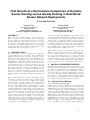
First Results of a Performance Comparison of Dynamic Source Routing
versus Greedy Routing in Real-World Sensor Network Deployments...................... 73
H. Frey, K. Pind
How to Take Advantage from Correlated Node Movement in
Mobile Sensor Networks......................................................................................................................... 77
A. Klein
Ghost: Software and Configuration Distribution for
Wireless Sensor/Actor Networks..................................................................................................... 81
M. Baunach
Positionierung und Sensor Web Enablement in Geosensornetzwerken.................... 85
K. Walter, A. Born
Self-Adaptive Load Balancing for Many-to-Many
Communication in Wireless Sensor Networks.......................................................... 89
M. Gonzalo, K. Herrmann, K. Rothermel
From Academia to the Field: Wireless Sensor Networks for Industrial Use.......... 93
R. Falk, H.-J. Hof, U. Meyer, Ch. Niedermeier, R. Sollacher, N. Vicari
Vergleichbarkeit von Ansätzen zur Netzwerkanalyse in
drahtlosen Sensornetzen...................................................................................................................... 97
J. Wilke, F. Werner, M. Bestehorn, Z. Benenson, S. Kellner, E.-O. Blaß
FRONTS - Foundations of Adaptive Networked Societies of Tiny Artefacts.........101
T. Baumgartner, A. Kröller, S. P. Fekete, C. Becker, D. Pfisterer
Vorwort
In dem vorliegenden Tagungsband sind die Beiträge des Fachgesprächs Drahtlose Sensornetze
2008 zusammengefasst. Ziel dieses Fachgesprächs ist es, Wissenschaftlerinnen und Wissenschaftler
aus diesem Gebiet die Möglichkeit zu einem informellen Austausch zu geben – wobei immer auch
Teilnehmer aus der Industrieforschung willkommen sind, die auch in diesem Jahr wieder teilnehmen.
Das Fachgespräch ist eine betont informelle Veranstaltung der GI/ITG-Fachgruppe „Kommunikation
und Verteilte Systeme“ (www.kuvs.de). Es ist ausdrücklich keine weitere Konferenz mit ihrem
großen Overhead und der Anforderung, fertige und möglichst „wasserdichte“ Ergebnisse zu
präsentieren, sondern es dient auch ganz explizit dazu, mit Neueinsteigern auf der Suche nach ihrem
Thema zu diskutieren und herauszufinden, wo die Herausforderungen an die zukünftige Forschung
überhaupt liegen.
Das Fachgespräch Drahtlose Sensornetze 2008 findet in Berlin statt, in den Räumen der Freien
Universität Berlin, aber in Kooperation mit der ScatterWeb GmbH. Auch dies ein Novum, es zeigt,
dass das Fachgespräch doch deutlich mehr als nur ein nettes Beisammensein unter einem Motto ist.
Für die Organisation des Rahmens und der Abendveranstaltung gebührt Dank den beiden
Mitgliedern im Organisationskomitee, Kirsten Terfloth und Georg Wittenburg, aber auch Stefanie
Bahe, welche die redaktionelle Betreuung des Tagungsbands übernommen hat, vielen anderen
Mitgliedern der AG Technische Informatik der FU Berlin und natürlich auch ihrem Leiter, Prof.
Jochen Schiller.
Berlin, im September 2008
Hartmut Ritter
Bug Hunting in Sensor Network Applications
Raimondas Sasnauskas, Jó Ágila Bitsch Link,
Muhammad Hamad Alizai, and Klaus Wehrle
Distributed Systems Group
RWTH Aachen University, Germany
{lastname}@cs.rwth-aachen.de
ABSTRACT
Testing sensor network applications is an essential and a difﬁcult task. Due to their distributed and faulty nature, severe
resource constraints, unobservable interactions, and limited
human interaction, sensor networks, make monitoring and
debugging of applications strenuous and more challenging.
In this paper we present KleeNet — a Klee based platform
independent bug hunting tool for sensor network applications before deployment — which can automatically test applications for all possible inputs, and hence, ensures memory
safety for TinyOS based applications. Upon ﬁnding a bug,
KleeNet generates a concrete test case with real input values
identifying a speciﬁc error path in a program. Additionally,
we show that KleeNet integrates well into TinyOS application development life cycle with minimum manual eﬀort,
making it easy for developers to test their applications.
1.
Starting with lint [8] tool nearly three decades ago, there has
been enormous eﬀort spent on the error removal in C programs. Many techniques have been developed ranging from
static code analysis, formal veriﬁcation, to full state model
checking. Numerous tools exist and are freely available to
use [4, 5, 7, 15]. Hence, our ﬁrst step was to employ them
for testing sensor network software written in widely spread
TinyOS platform [12]. We encountered the following problems due to which the available tools are mostly not used at
all, and the developers fall back on manual code debugging
techniques:
• Sensor network applications are tightly integrated with
the whole operating system leading to time-consuming
manual code modiﬁcation in order to perform the actual testing.
• Most of the tools perform only static code analysis
with limited support for C semantics. Since sensor
network applications mainly process data from the environment, possible runtime errors might stay undetected.
INTRODUCTION
As with any software, testing of wireless sensor network applications is an essential part of development life cycle. The
main goal of this engineering task remains the same: ﬁnding
and ﬁxing program bugs as early as possible.
Currently, sensor network application developers are confronted with a number of domain speciﬁc complications. The
constrained memory and CPU resources on sensor nodes result in using low-level, type-unsafe languages without dynamic type checking and memory protection. Similarly, because the applications are highly data-ﬂow oriented, the correct exception handling at full coverage is a challenging task.
Moreover, due to highly distributed and faulty nature of sensor nodes, some of the program bugs are detected only after
the software is deployed.
C language has been the main choice for developing sensor
network applications. It provides great ﬂexibility, expressiveness, and in particular, the required low resource footprint. However, the absence of dynamic type checking necessitates very careful programming because many sensor OS’s
do not support memory protection. We argue that, besides
the particular sensor application semantic, the majority of
bugs comes from general programming ﬂaws such as memory out-of-bounds references, null pointer dereferences, or
wrong type conversions. Especially, the widely used casting
between pointers to structures may lead to well-hidden type
errors. But in most cases, the given language features are
simply misused by novice programmers.
• None of the tested tools can oﬀer a push-button bug
ﬁnding technology and the usage learning curve is mostly
too steep for a typical developer.
We have discovered that recent research eﬀorts in the area
of C code checking are now targeting the usability and full
automation as primary design goals [1, 2]. The philosophy is
to detect only deﬁnite errors, but automatically, at full execution path coverage, and with minimum manual eﬀort by
employing symbolic checking techniques [9]. We think that
these eﬀorts could ﬁnally achieve the integration of sound
testing tools into the application development process.
2.
RELATED WORK
To the best of our knowledge, currently there are no frameworks for automatic bug detection in sensor network applications before deployment at bit-accurate C semantics. For
bringing memory safe executions of applications at runtime,
we only know of the related eﬀorts [6, 10], where the sole
representative with ﬁned-grained memory safety at C level
is Safe TinyOS.
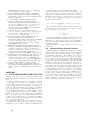
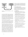
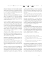
Safe TinyOS adds dynamic memory checks during compilation which allows to catch unsafe pointer and array operations without corrupting the RAM. Overall, this results in
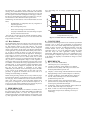
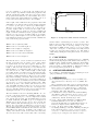
Features
Automatic code instrumentation
Target platform independence
Assembly level bug detection
Oﬀ-line bug detection
All possible input values checked
Automatic test case generation
Runtime safety enforcement
No additional resource usage
Safe TOS
KleeNet
−
−
+
−
−
−
+
−
+
+
−
+
+
+
−
+
Table 1: Comparison: Safe TinyOS and KleeNet
13% increase in the code size and 5.2% increase in CPU usage. As with any dynamic assertion checking, Safe TinyOS
can detect program bugs only eventually after the software is
deployed. Therefore, still many corner-case bugs circumvent
this testing technique. KleeNet, on the other hand oﬀers
oﬄine bug detection with automatic code instrumentation.
In doing so, it doesn’t consume any system resources and
ensures memory safety by treating the inputs symbolically
i.e. checks any program variable for its all possible input
values. As the core engine of KleeNet interprets a virtual
instruction set, it cannot detect hardware platform dependent assembly level bugs nor enforce runtime memory safety.
Thus, KleeNet complements the beneﬁcial features of Safe
TinyOS allowing altogether even more rigorous application
testing (see Table 1).
Overall, we make following contributions: First, we integrate
an eﬀective bug ﬁnding tool into the event-driven TinyOS
programming model with usability as a primary goal. Second, we show that, apart from the general checks already
available, Klee can easily be extended to incorporate further
checks useful for testing sensor network applications. And
third, we practically demonstrate that sound testing techniques can be used throughout the application development
process with minimum manual eﬀort.
3.
SYSTEM OVERVIEW
In this section, we present an overview of our system. First,
we introduce Klee, which we use for symbolically executing
C applications. We continue by discussing how we automatically instrument source code without the help of application developers. We conclude this section by presenting our
extension of Klee to enable struct type checking in sensor
network applications.
3.1
Klee
Klee is a symbolic execution tool for C programs based on
LLVM [11]. In contrast to common runtime testing where
the program input is (manually) generated, Klee runs the
code on symbolic input initially allowed to be “anything”.
The programmer only needs to specify which memory locations in his code are input-derived, e.g. an incoming network
packet. During code execution, all paths and operations on
symbolic variables are tracked. If a bug is detected, Klee automatically generates a test case with concrete values causing the bug. For example, consider a simple application code
in listing 1 and the associated KleeNet output in listing 2.
At the current state of its implementation, Klee reports only
memory reference and division by zero errors. It has been
developed to be scalable and to support all sorts of unsafe
type operations including pointer casts and pointer arithmetics.
...
c a l l Timer1 . s t a r t P e r i o d i c ( 5 0 0 ) ;
...
int a [ 1 0 ] ;
unsigned i ;
klee make symbolic name(&i , sizeof ( i ) , ” i ” ) ;
event void Timer1 . f i r e d ( )
{
c a l l Leds . led1Toggle ( ) ;
// here we v i o l a t e memory s a f e t y
// on the 11 th s i g n a l of t h i s event
i f ( i < 11)
a [ i++] = 1 ;
}
...
Listing 1: Array index out of bounds bug
$ make k l e e n e t t e s t
KLEE: ERROR: memory e r r o r : out o f bound pointer
$ make k l e e n e t d i s p l a y
BlinkFailC$i : ’ 10 ’
Listing 2: KleeNet detects the memory error and
generates a concrete test case
3.2
Automatic Code Instrumentation
As discussed earlier, one of the major limitations associated
with most software testing tools is the lack of user friendly
interfaces. Most of the available tools are either not properly
integrated into software development process, or they even
require manual code modiﬁcations for testing the code.
One of our major design objectives is to provide an easy to
use bug ﬁnding tool for sensor network applications which
is strongly integrated in the software development life cycle.
For this purpose, we use grammar based automatic code
instrumentation. We extend ANTLR [13] based GNU C
grammar to automatically insert symbolic annotations (i.e.
to mark the memory locations to be checked by Klee) in
the C source code. The user only needs to provide a high
level conﬁguration stating the variable names that has to
be checked inside the code. However, providing a conﬁguration to insert annotations in the code to perform additional
checks is optional, as our solution performs some built-in
checks to detect common bugs in sensor network applications. For example, struct type cast checking (discussed in
section 3.3) and memory checks on received packet buﬀers.
3.3
Struct type checking
Type conversions in C using type casts is a very common
practice, and, deﬁnitely not an error. But since type safety
is not guaranteed, programmers can interpret each memory
region to be of any type. Especially, the casts between pointers to diﬀerent structure types make the code maintenance
diﬃcult [3, 14].
One of the main objective of sensor network applications is
to collect and process data from the sensors. The received
data is at ﬁrst available only as an untyped bit stream. Afterwards the pointer to this data is casted to a known structure type based on particular bit ﬁelds. During code execution further casts on this memory location are executed. We
have extended the functionality of Klee to check the struct
type equality during casting operations. This check is optional, but nevertheless the warnings as shown in listing 4
are useful and facilitate program comprehension.
...
NewRoute∗ msg = (NewRoute∗) payload ;
// message processing
c a l l Queue . enqueue (msg ) ;
...
RouteUpdate∗ msg =
( RouteUpdate∗) c a l l Queue . dequeue ( ) ;
// f u r t h e r message processing
...
��
��
��
��
��
��
$ make kleenet
��
��
��
��
��
��
��
$ make kleenet test
��
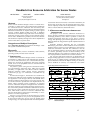
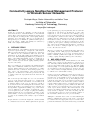
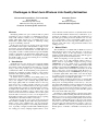
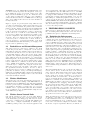
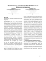
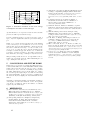
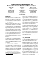
Figure 1: Integration of KleeNet into TinyOS platform
Listing 3: Casting between pointers to diﬀerent
structure types
our approach can easily be integrated into any other sensor
network development platform and operating system.
$ make k l e e n e t t e s t s t r u c t
KLEE: WARNING: Struct types don ’ t match
KLEE: %s t r u c t . NewRoute∗ −> %s t r u c t . RouteUpdate∗
5.
Listing 4: KleeNet warnings
4.
INTEGRATION INTO TINYOS
We decided to integrate Klee into TinyOS by adding a virtual KleeNet platform based on the TinyOS null platform.
This approach allows us to easily add diﬀerent modules to a
platform, that automatically marks sensor value input and
incoming packets as symbolic.
Since TinyOS applications are event-driven, parts of the
code are executed only eventually after particular events are
ﬁred. In order to cover all possible program control ﬂow
paths during testing, we have extended our virtual platform
with an automatic event signaling mechanism. Once an application is booted, all implemented events are signaled and
processed. Finally, after processing the last event TinyOS
scheduler is stopped.
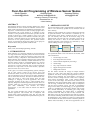
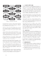
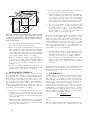
Figure 1 shows an overview of KleeNet’s build process. First,
a user can optionally specify in a conﬁguration ﬁle which
variables in his code should be marked as symbolic. For this
purpose we parse the C-code after NesC compilation and
insert calls to klee_make_symbolic function. Second, all
incoming packet buﬀers are also marked symbolic automatically. Third, the instrumented code is then passed to Klee
which builds the C-object ﬁle. Finally, Klee interprets this
object ﬁle and terminates when no bug is detected. Otherwise a test case with real input values is automatically generated. Running this concrete test case with the unmodiﬁed
version of the code will cause the deployed sensor network
application follow the same path and hit the same bug.
Please note that, as we apply code instrumentation to C
source-code, therefore, this process is neither bound to a
certain hardware platform nor to TinyOS and NesC. Hence,
EVALUATION
We ﬁrst checked the BlinkFail application from the TinyOS
source repository. It is used to test if the Safe TinyOS
toolchain installation is working properly. After marking
the array index variable as symbolic we immediately detected the known out of bound pointer error.
...
int r a t i o ;
event message t∗ Receive . r e c e i v e ( message t∗ bufPtr ,
void∗ payload , u i n t 8 t len ) {
i f ( len != sizeof ( r e c e i v e f a i l m s g t )){ return bufPtr ; }
else {
r e c e i v e f a i l m s g t ∗ rcm=
( r e c e i v e f a i l m s g t ∗) payload ;
// p o s s i b l e d i v i s i o n by zero here ,
// depending on received message
r a t i o = rcm−>good / rcm−>t o t a l ;
return bufPtr ;
}
}
...
Listing 5: Possible division by zero error
$ make k l e e n e t t e s t
KLEE: ERROR: d i vi d e by zero
Listing 6: KleeNet detects the div by zero error
In listing 5, we demonstrate the usability of KleeNet for
ﬁnding possible bugs without annotating application source
code any further. A received message is processed without
sanitizing the received message which is a typical fault of
students new to programming. KleeNet rapidly detects this
mistake and warns the developer (Lst. 6).
Overall, after our initial tests, we have conﬁrmed the following key beneﬁts of KleeNet:
[3]
Usability: A programmer can test the code with minimum
manual eﬀort and without any previous knowledge about
the checking tool.
[4]
Coverage: KleeNet covers all possible execution paths and
checks all possible data values before application deployment.
[5]
Integration: KleeNet is invoked by simply adding an extra
build ﬂag enabling the permanent code checking during the
application development process.
[6]
Eﬃciency: It is fast for everyday use.
6.
CONCLUSION AND FUTURE WORK
In this paper, we presented our technique and prototype
implementation for automatic testing of sensor network applications before deployment. It is important to fully test
(taking all possible inputs into account) embedded applications, such as sensor networks, where the cost of occurring undetected errors after deployment could be fatal. We
have demonstrated that it is possible to close the gap between the testing and development community by providing
a user-friendly, automated bug ﬁnding tool which is strongly
integrated in the system development life cycle. We gave an
overview of our system design and of the preliminary evaluation results achieved.
Strenuous deployment requirements and resource constrained
nature of sensor hardware, e.g. inadequate power supply and
limited computational power, demand even more rigorous
testing of sensor network applications. Incorporating further useful checks in Klee, such as runtime monitoring of
long loops and computationally intensive tasks by adding
time annotations, is future work. Similarly, verifying the distributed behavior of sensor network protocols — such as correct state transitions — remains to be addressed. Moreover,
apart from TinyOS, we will apply our solution to other sensor network operating systems and development platforms.
7.
REFERENCES
[1] D. Babic and A. J. Hu. Calysto: scalable and precise
extended static checking. In ICSE ’08: Proc. of the
30th international conference on Software engineering,
2008.
[2] C. Cadar, V. Ganesh, P. M. Pawlowski, D. L. Dill,
and D. R. Engler. EXE: automatically generating
10
[7]
[8]
[9]
[10]
[11]
[12]
[13]
[14]
[15]
inputs of death. In CCS ’06: Proc. of 13th ACM conf.
on Computer and communications security, 2006.
S. Chandra and T. Reps. Physical type checking for C.
SIGSOFT Softw. Eng. Notes, 1999.
H. Chen and D. Wagner. MOPS: an infrastructure for
examining security properties of software. In CCS ’02:
Proc. of the 9th ACM conference on Computer and
communications security.
E. Clarke, D. Kroening, and F. Lerda. A Tool for
Checking ANSI-C Programs. In Tools and Algorithms
for the Construction and Analysis of Systems (TACAS
2004), 2004.
N. Cooprider, W. Archer, E. Eide, D. Gay, and
J. Regehr. Eﬃcient memory safety for TinyOS. In
SenSys ’07: Proc. of the 5th international conference
on Embedded networked sensor systems, 2007.
T. A. Henzinger, R. Jhala, R. Majumdar, G. C.
Necula, G. Sutre, and W. Weimer. Temporal-Safety
Proofs for Systems Code. In CAV ’02: Proc. of the
14th International Conference on Computer Aided
Veriﬁcation, 2002.
S. Johnson. Lint, a C program checker. Computer
science technical report 65, Bell Laboratories, 1977.
J. C. King. Symbolic execution and program testing.
Commun. ACM, 1976.
R. Kumar, E. Kohler, and M. Srivastava. Harbor:
software-based memory protection for sensor nodes. In
IPSN ’07: Proc. of the 6th international conference on
Information processing in sensor networks, 2007.
C. Lattner and V. Adve. LLVM: A Compilation
Framework for Lifelong Program Analysis &
Transformation. In CGO ’04: Proc. of the
international symposium on Code generation and
optimization, 2004.
P. Levis, S. Madden, J. Polastre, R. Szewczyk,
K. Whitehouse, A. Woo, D. Gay, J. Hill, M. Welsh,
E. Brewer, and D. Culler. TinyOS: An Operating
System for Sensor Networks. In Ambient Intelligence.
2005.
T. J. Parr and R. W. Quong. Antlr: a predicated-ll(k)
parser generator. Software: Practice and Experience,
July 1995.
H. Shen, J. Wang, L. Ping, and K. Sun. Securing C
Programs by Dynamic Type Checking. In ISPEC,
2006.
N. Volanschi. A Portable Compiler-Integrated
Approach to Permanent Checking. In ASE ’06: Proc.
of the 21st IEEE/ACM International Conference on
Automated Software Engineering, 2006.
Over-the-Air Programming of Wireless Sensor Nodes
Martin Stemick
[email protected]
Anthony Boah
[email protected]
Hermann Rohling
[email protected]
Hamburg University of Technology
Eissendorfer Str. 40
21073 Hamburg
ABSTRACT
Self-organizing Wireless Sensor Networks (WSNs) have gained
much attention in recent research and industrial activities. Such
WSNs enable measurements and information dissemination over
large areas. A common node in a WSN is usually equipped with a
microcontroller and a radio transceiver. A challenge in large
networks is to keep the firmware of the nodes up to date. Once the
network is deployed, it is hardly possible to access every node
physically and to upload a new firmware. Therefore, this paper
describes a technical solution for this problem using the radio
transceiver for the upload procedure. The presented solution
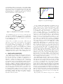
focuses on heterogeneous WSNs that contain several groups of
nodes and where each group fulfills a different task.
Keywords
WSN, OTAP, Network Reprogramming, AirFlash.
2. AIRFLASH CONCEPT
In a lab environment a node is reprogrammed by connecting it via
cable to a PC that directly uploads the new firmware into the
node’s memory.
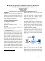
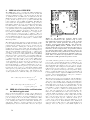
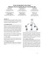
Instead of a cable, AirFlash uses a wireless connection to the node
to upload the firmware. This connection is established by a so
called Gateway node, which is connected to the PC via a serial
port. The Gateway then sends out the firmware image to an
addressed node. The node will receive the image, load it into its
memory and execute it. These are the main functions of the
AirFlash application. These functions are controlled by a host
software running on the PC. (see Figure 1).
Host
Software
1. INTRODUCTION
WSN technology is a promising candidate to provide monitoring
over large areas and for long time periods. The network consists
of a large number of small and inexpensive nodes. Each node
contains a sensing-, computation- and communication unit. The
WSN technology will be applied in dangerous areas where human
beings have no access. Therefore, network maintenance or even
firmware updates cannot be accomplished based on a physical
access to the nodes and to the network. But the nodes can be
accessed over a wireless connection. Thus, in order to update the
firmware on a single node or in the entire network, a procedure
based on wireless access will be used.
In this paper, an Over-the-Air-Programming (OTAP) technique
will be used, which is based on the wireless access and
transmission scheme. In this case an image of the node firmware
will be transmitted via the wireless link. The image information
will be stored inside the node. The node will then load this new
image and execute it. These tasks already imply the main
challenges in designing an OTAP application. The OTAP
application presented in this paper is called AirFlash and is
especially designed to maintain experimental networks. These are
networks, which vary very much in size and are reprogrammed
quite often. Additionally, such networks are mostly
heterogeneous, i.e. the nodes inside the network run different
applications.
The next section introduces the concept and features of the
AirFlash application. This includes also a comparison with
already known OTAP applications. After that, the used node
platform is introduced and important implementation aspects are
addressed.
Gateway
Node
Figure 1. Overview of AirFlash
For experimental WSNs a few more features are needed, which
will be listed below:
1.
Several images on a node
2.
ID of image names and versions
3.
Check AirFlash-compatibility of an image
4.
Golden Image
5.
Easy setup of nodes for AirFlash
6.
Support heterogeneous networks
7.
Background Execution
The first feature describes the storage of multiple firmware
images on a node, where each image may contain a different
application. This allows selecting which application to run by a
simple wireless command. The second feature is necessary to
trace the versions of images stored on a node. This is especially
useful during development, when a node contains different
versions of the same image. The features three and four avoid
malfunctions while using AirFlash. Before a node is programmed
with an image, AirFlash must check the image for compliance
with the current AirFlash version, such that no incompatible
images will be loaded. A Golden Image [1] is an application that
resides in a predefined part of the node’s memory and provides
basic AirFlash functionality. If something goes wrong during
wireless reprogramming, the Golden Image is automatically
executed on the node. Thus, the node will stay accessible. The
fifth feature is the one-step preparation of the node for AirFlash.
This includes formatting of the nodes memory and installation of
the Golden Image. Also, as feature six points out, an image should
not be flooded to all nodes in the network. It should be possible to
address nodes individually, so that various applications can be
11
present inside the WSN. And finally, since AirFlash is only used
for reprogramming, while the node normally executes its usual
measurement application, AirFlash should stay in the background
if not used and claim as few resources as possible.
All these features named above are highly useful for running and
maintaining a WSN. They are all included in the AirFlash
application discussed in this paper. This feature combination is
unique to the presented AirFlash and is not found in other OTAP
implementations like Crossbow OTAP [2] or Deluge T2 [3]. For
example neither Crossbow nor Deluge support feature three and
five. Deluge additionally does not support feature six. And
Crossbow has the disadvantage that it consists of proprietary
code.
These are some of the reasons why AirFlash was created. The
implementation of all the listed features into AirFlash will be
introduced in the following sections.
3. PLATFORM
AirFlash is realized and tested for the IRIS node [4] as an
example. This is a wireless node with a 2.4 GHz radio transceiver
and an ATmega1281 microcontroller that contains 128kB of
internal program memory (Flash) and 4kB of internal EEPROM
[5]. Additionally, the IRIS node provides 512kB of external flash
memory, which will be used to store multiple firmware images.
AirFlash partitions the external memory into three so called slots
of 120kB for firmware images and a fourth slot of 20kB for the
Golden Image. The remaining 132kB can be used by data logging
applications. For programming of the node the open-source
framework TinyOS 2.x is used [6]. The choice for TinyOS was
made, since it provides powerful high-level interfaces to access
the node’s hardware.
4. AIRFLASH IMPLEMENTATION
At the node’s location, there are three basic tasks, which must be
performed by AirFlash:
-
Receive image via wireless transfer
-
Store image in external slot
-
Load image from slot to program memory
For the last task, the microcontroller’s internal and external
memory must be accessed. For this purpose, usually a so called
bootloader application is used. This bootloader resides in a
dedicated partition (8kB) of the program memory of the
ATmega1281 and is able to access the remaining 120kB of
memory and execute applications therein. The bootloader is also
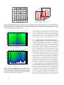
able to access the external memory (see Figure 2). Since the
partition dedicated for the bootloader is too small to contain the
complete AirFlash functionality, task one and two of the above
list must be performed by an additional software module. Such an
AirFlash module that controls the wireless image transfer must be
included into the node’s main application. There it stays in the
background and is only activated when awoken by a wireless
command. If the AirFlash module is woken up, it can receive an
image via radio and store it into a memory slot. By another
command, the module can afterwards invoke the bootloader that
loads the image from the slot, overwrites the old application
(including module) in the program memory and starts the new
application contained inside the image (see Figure 2).
12
Node
Ext. Memory
AirFlash
module
Slot 0
Slot 1
Slot 2
Bootloader
GoldenImg
Figure 2. AirFlash components inside node
The implementation of the bootloader and the AirFlash module
will be discussed in the following.
4.1 Bootloader
The bootloader has the main purpose to read an image from the
external memory, process an error check and then write the image
file into the upper part of the microcontroller’s program memory.
The bootloader is invoked from the main application by setting
the program counter to the bootloader’s start address. The
information from which slot to load an image from the external
memory is passed to the bootloader via a command flag in the
microcontroller’s EEPROM. These flags are also used to signal
the application if the image was successfully loaded. This
information has to be passed through the EEPROM since the
RAM of the microcontroller will be reinitialized when changing
between main application and bootloader. Before starting to write
the image into the internal program memory, the bootloader
checks a flag in the EEPROM, if a previous write operation
failed. Additionally, all CRCs of the image are verified. To this
end, an image slot inside the external memory is organized in
pages of 256 bytes where each page contains a 2 byte CRC. A slot
also contains an additional 2 byte CRC, which is used to verify
the CRCs of all pages. Thus, the integrity of an image can be
guaranteed. If everything is correct, the selected image is written
to the program memory. The bootloader then sets the status flags
and resets command flags in the EEPROM and the program
counter is set to the start address of the transferred image. The
application inside the image is then executed.
If an error is detected in the image to load, the bootloader will not
write it to the program memory and sets the respective error flags
in the EEPROM. Then the control is given back to the main
application.
There is still the possibility that an undetected error occurs while
writing to the program memory. If this happens and the program
counter is reset to the application, it will skip these illegal code
parts and return to the bootloader. There, the exceptional
invocation is detected, since the command flags are not properly
set. Then the bootloader loads the Golden Image. The fourth slot
in the external memory is reserved for this. The Golden Image
contains the main AirFlash functionality and provides a fall-back
solution, if something fails during reprogramming.
Still, it has to be discussed, how the image packets are received at
the node and how they are written into the slots of the external
memory. This is the task of the AirFlash module, which is
described in the following.
4.2 AirFlash Module
The AirFlash module is implemented as a TinyOS component and
therefore can be integrated into any TinyOS application. The
integration of this module needs less then 6kB of additional
program memory. It uses the node’s radio to receive image data
from the host PC and to transmit status information. The radio
device is shared between the AirFlash module and the main
TinyOS application. The main application possesses the master
control over the radio. The request and release of the radio by
AirFlash is signaled to the main application by events. The
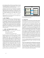
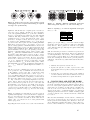
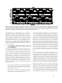
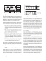
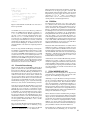
AirFlash module can assume three main states (see Figure 3): In
order to save resources, the AirFlash module works in the
background of the main application and is mostly in the sleep
state.
booted
timer event
Receive
Packet
Write packet
to page buffer
Page
complete
Verify
page
Success
Write page
buffer to
external
memory
Failed
Page
incomplete
Send
NACK
Figure 4. Image transfer from the node’s perspective
AirFlash ID
Packet ID
timer event
Sleeping
Send
ACK
Peeking
Command
Storage page
Storage page bias
Data size
sleep packet
or timeout
Wide
awake
wakeup
packet
AirFlash
packets
Figure 3. Sleep-wake cycle of AirFlash module
The module periodically enters the peeking state to listen for
AirFlash-related packets. If nothing is received, the module goes
to sleep after a while. If a so called enumeration packet is
received, the module sends a status message back to the host. If a
wakeup packet is received, the module steps into the “Wide
awake” state. Inside this state it is ready to receive image data and
to write it into the external memory. The module goes to sleep
again if the host sends a sleep packet or if a timeout occurs.
In the following, the AirFlash protocol that handles the image
transfer between host and node will be explained. First, the host
transmits a wakeup packet, in order to put the node into the “Wide
awake” state. The awoken node answers to the host. Then the
transmission of the image file can start. This process is depicted
in Figure 4. Since the image is up to 120kB in size, it must be
fragmented. Each fragment contains 256 Bytes, which is also the
size of a page in the memory. Each AirFlash packet (see Figure 5)
contains 16 bytes of image data, a so called subfragment. Thus, to
transmit one fragment of 256 bytes, 17 AirFlash packets are
necessary, where the last packet contains a CRC checksum to
verify the fragment.
Data
CRC16
Figure 5. AirFlash packet format
All received subfragments are buffered in the RAM of the node.
The CRC from the 17th packet is then used to verify the whole
fragment. If verification fails, a NACK packet is sent to the host
and the whole fragment is retransmitted. If verification is
successful, the fragment is written to the respective page of the
external memory and an ACK packet is sent to the host. This
buffering of whole fragments of the image has two benefits: First,
only a few ACKs are needed, which improves transfer speed. And
second, most data corrections take place inside the RAM which
extends the lifetime of the external memory.
When the image transfer is finished, the host can invoke the
bootloader by sending a special command. This command also
contains the number of the slot to be loaded. This information is
stored in the EEPROM to preserve it for the bootloader.
After the description of the transfer process, a closer look at the
AirFlash packet is taken:
The first field contains the AirFlash ID that distinguishes between
up- and downlink of an AirFlash connection. Thus, other nodes
with AirFlash connections are not disturbed by packets from other
nodes.
13
Summarizing, the main features of the AirFlash module are listed
below:
-
Implementation as component, thus easy integration in
TinyOS applications
-
Runs as background process
-
Writes received images to external memory
-
Can jump to bootloader after successful image reception
-
Provides AirFlash status for host
This leads us to the last part of the AirFlash application, namely
the host software. This software runs on a PC and controls the
image transfers to all nodes.
4.3 Host Software
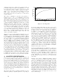
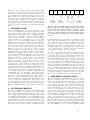
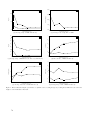
for a fixed image size. In average, a transfer rate of 1,1 kB is
achieved.
16
Image size (kB)
The Packet ID is a simple counter, which is used for packet
ordering. The Command field contains commands to the AirFlash
module. The Storage page identifies the current page to write and
the offset points to the actual subfragment of this page. It follows
the data size and the data field, which can contain up to 16 bytes.
The last field is a CRC checksum to detect packet errors.
32
64
120
0
20
100
60
80
40
Image transfer time (sec)
120
Figure 6. Transfer times for various image sizes
6. CONCLUSION
The implementation of the host software can be divided into three
main parts: The first part is an interface to the serial port of the
PC that transmits packets to the radio Gateway. The second
component processes the AirFlash protocol. The last component
realizes a user interface. In this paper, only the basic functionality
of this application is presented. For further details please refer to
[7]. In order to transfer an image to a node, the image file is
loaded from the PC’s hard drive into the application. The integrity
of the image is verified by checksums. It is also checked, if the
image would fit into a slot. In a further check, the so called
AirFlash signature (10 bytes) is read from the image file which is
only present in AirFlash-capable images. If this signature is
missing, the image will not be transferred, since the node will not
be reachable via AirFlash after being reprogrammed with a nonAirFlash image. A second signature contains information about
the AirFlash version the image was compiled with. This ensures
that also the host software is compatible to the image.
Additionally, the AirFlash version of the image must be the same
as the version of the Golden Image on the node. The only
possibility to upgrade the AirFlash version on the node is to
exchange its Golden Image via AirFlash.
The discussed AirFlash application is well suited for experimental
networks, since it allows the programming of heterogeneous
networks. The use of a Golden Image makes the application very
reliable if used in the field. An additional advantage is that the
AirFlash module can be easily integrated into any TinyOS
application. There, it stays in the background when not needed
and thus keeps the main application running smoothly.
Furthermore, additional features can be easily implemented, since
the TinyOS part is completely open source. A feature that is going
to be added is the capability to disseminate an image to a whole
WSN at once.
Before starting the image transfer, the necessary number of pages
inside the node’s memory is calculated as well as CRC checksums
for each page. Then a command to erase the selected slot on the
node is sent. After an ACK is received the image transfer starts.
This process is analogous to the one described in chapter 4.2. If
an error occurs that cannot be handled by the protocol, the process
is aborted and must be restarted via the user interface.
[4] Crossbow Technology. 2008. IRIS data sheet. (Retrieved
June 02, 2008). URL=http://www.xbow.com/Products/
productdetails.aspx?sid=264
5. PERFORMANCE
Finally, the transfer performance of AirFlash is evaluated. To test
the upload speed, images of 16kB, 32kB, 64kB and 120kB were
transferred multiple times to a node. The elapsed times were
collected and averaged. If the radio channel is not frequently used
by other applications, the transfer durations are almost constant
14
7. REFERENCES
[1] Hui, J., et al. 2008. TOSBootM.nc.
URL=http://tinyos.cvs.sourceforge.net
[2] Crossbow Technology. 2008. XMesh User’s Manual.
(Retrieved June 05, 2008). URL=http://www.xbow.com/
Products/productdetails.aspx?sid=154
[3] Chlipala, A. 2003. Deluge: Data Dissemination for Network
Reprogramming at Scale. Technical Report. UC Berkeley
[5] Atmel Corporation. 2007. ATmega1281 data sheet.
(Retrieved June 05, 2008) URL=http://www.atmel.com/dyn/
resources/prod_documents/doc2549.pdf
[6] UC Berkeley. 2004. TinyOS Community Forum. (Retrieved
June 05, 2008). URL=http://www.tinyos.net
[7] Boah, A. 2008. Over-the-Air-Programming of Wireless
Sensor Nodes. Project Thesis. Hamburg University of
Technology.
Deadlock-free Resource Arbitration for Sensor Nodes
Michael Baar
Heiko Will
Jochen Schiller
Adam Dunkels
Freie Universität Berlin
Berlin, Germany
Swedish Institute of Computer Science
Box 1263, SE-164 29 Kista, Sweden
{baar,hwill,schiller}@inf.fu-berlin.de
[email protected]
Abstract
Sensor network hardware designs consist of a central microcontroller, to which sensors and communication peripherals
are connected. Resource arbitration and concurrency management must be implemented in software. Existing hardware
arbitration mechanisms use explicit locking to protect against
resource conflicts. Explicit locking may lead to deadlock,
which must be avoided for long-term sensor network deployments. We present a power-saving resource arbitration architecture that is deadlock-free, portable, and resource-efficient.
The architecture explicitly manages inter-device dependencies
to know what devices to power down.
Categories and Subject Descriptors
D.4.7 [Operating Systems]: Organization and Design - Realtime systems and embedded systems
Keywords
hardware abstraction, resource arbitration, fault-tolerance,
operating systems, wireless sensor networks
1 INTRODUCTION
Sensor network hardware designs consist of a central microcontroller to which sensors and communication peripherals, such as radio transceivers, are connected. Because peripherals are used both by applications and by the operating
system, access to the peripherals must be controlled with an
arbitration mechanism.
We present a power saving resource arbitration architecture and hardware abstraction layer (HAL) that provides
portability of applications and drivers between different
hardware platforms. Unlike existing resource arbitration
architectures [3] [7], our architecture is deadlock-free by
design.
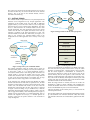
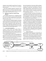
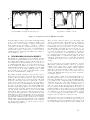
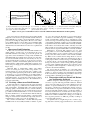
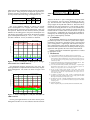
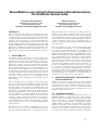
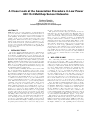
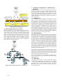
As illustrated in Figure 1, introduction of a hardware abstraction layer (HAL) increases portability of operating system
and application code through common, well-defined device
interfaces. High-level device drivers can reuse low-level drivers and do not need to provide their own implementation. To
further reduce operating system complexity, we integrate
resource arbitration and power management into the HAL as
part of the operating system. Most operating systems for wireless sensor nodes provide no hardware abstraction at all. Even
those who do, require cooperative interaction of user applications, which need to take care of resource arbitration. This
increases development overhead and vulnerability to uncooperative or erroneous applications.
Energy is a scarce resource on wireless devices. To reduce
the energy consumption, every circuit and peripheral has to
be powered off when they are not used. An optimal power
saving strategy can only be implemented when the dependen-
cies between devices are known; to switch off a shared bus, all
devices that use the bus must be switched off first. Our architecture explicitly encodes device dependencies to determine
when to switch off devices and shared busses.
2 A DEADLOCK-FREE RESOURCE ARBITRATION
ARCHITECTURE
The purpose of our resource arbitration architecture is
both to provide a hardware abstraction layer on top of the
underlying hardware, and to make it possible to switch off
hardware peripherals when they are not used to conserve
energy. The operating system and its applications can run on
different platforms using platform-specific implementations of
the HAL.
Stackable hardware platforms like the ScatterWeb
MSB-430 [1], that allow run-time addition of new boards and
hardware devices, present a novel challenge for the resource
arbitration architecture and HAL. The architecture must be
able to dynamically adapt to new device drivers being added
at run-time, potentially stored in on-board memory of the
additional hardware. Our architecture supports this by using
one-way dependencies and allows for run-time extension.
Our resource arbitration architecture is deadlock-free by
design. Existing approaches to resource arbitration for sensor
nodes [7] rely on explicit locking to determine when a peripheral should be switched off. Explicit locking can, however,
lead to deadlock. In contrast, our architecture uses atomic
System Design without Hardware Abstraction
Operating System and Applications
Radio Driver
SD-Card Driver
SPI Driver
SPI Driver
USART0
SPI
Radio
Compass
Driver
SPI Driver
Timer
UART Driver
USART1
SPI 2 MHz
SD-Card
SPI
Compass
Circuit
UART 56 kb/s
Terminal
Circuit
Clock System
Terminal
Timer
System Design with Hardware Abstraction
Operating System and Applications
Radio
Storage
Driver
Compass
Driver
HAL (Low-level Drivers, Resource Arbitration, Power Management)
Hardware Platform
Figure 1.
System architecture without and with hardware
abstraction layer
15
device. Each virtual device may require a different configuration of the shared resource such as data rate or protocol. Virtual device hubs contain all state information necessary for
multiplexing a shared device entity between an arbitrary
number of virtual devices. A single virtual device can be selected as default and will be active, whenever no other device
is active. The device selection is also used to forward interrupts to the right virtual device. A hub does not have a list of
connected devices, which allows introducing new virtual
devices dynamically at runtime.
A virtual device entity is an abstract software device. It is
specialized by virtual device classes and is not intended to be
used stand-alone. It extends the device entity. In this way the
virtual device becomes a unique device entity itself, can reference its dependencies and provide its own power and configuration management. It can be connected to a virtual device
hub, which then functions as a switching facility for all virtual
devices operating on the same shared device.
A virtual device class represents a set of virtual device entities with a common interface. Usually a common functionality
is also assumed. Typical classes found on embedded devices
would be serial byte I/O (e.g. communication ports, peripheral
connections) or memory (e.g. EEPROM, external flash card).
Depending on the implementation, access to the underlying
hardware can be shared, exclusive, virtualized or emulated.
To create a virtual device class the virtual device entity is
extended to a virtual device class with its own class specific
set of methods, callbacks, configuration and state. Callbacks
will usually be triggered by interrupts and are directly forwarded to a consumer. State is dynamic information, while
configuration is static. A virtual device class has a well known
set of methods which is implemented platform dependently.
From outside driver code, virtual devices are strictly to be
accessed only by the API.
operations to ensure deadlock-free operation. Every access to
a hardware resource, such as reading a sensor or sending a
packet over the radio, is atomic and cannot be interrupted by
another operation.
The resource arbitration architecture does power management of all hardware peripherals by switching off peripherals when they are not used. The architecture has knowledge of when devices can be powered off because it keeps
track of device dependencies and all access to peripherals
goes through the resource arbitration architecture.
2.1
Hardware Devices versus Virtual
Devices
Our hardware abstraction layer can implement device
drivers for devices that do not have a hardware equivalent.
This is useful for simulation or application development without access to the target hardware. We refer to all software
devices that may or may not have their representation in
hardware as virtual devices.
Virtual devices can be implemented using four techniques:
emulation, virtualization, or layering. Emulation is used when
no device of the desired class exists. The device functionality is
either emulated with an existing hardware device or simulated in software. Virtualization is used to increase the number of devices of a specific type. A larger number can be provided by software multiplexing. Multiplexing is done transparently to the application. Layering is used when one or more
hardware devices provide functionality that can be combined
or extended to a more powerful high-level device.
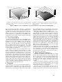
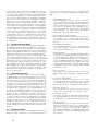
2.1.1
Structural Design Elements
Hardware devices are shared resources that usually correspond to physical devices. Each hardware device is
represented by a unique device entity in software. Different
method implementations are used to access a hardware device. This is useful for devices that can handle more than one
protocol. Each implementation can be used by multiple virtual
devices to minimize platform specific code.
We use device entities to model inter-device dependencies
and to provide per-device power control. Dependencies are
modeled as trees. Each device entity keeps a list of devices it
depends on. The owner marks device entities when the device
entities are in use. Root entities are owned by virtual device
entities and descendants are owned by their root.
We use virtual device hubs to implement device sharing.
Different virtual devices may operate on the same shared
extends
Virtual Device Class
Events
Device State
Device Config.
depends on
0..1
Methods
2.1.2
Using Virtual Devices
The structures we discussed so far can be kept slim to be
implemented on a resource limited device without much impact on usability. However, defining an adequate interface
specification for virtual device classes that fulfils our requirements, uses only a small amount of memory and still can be
implemented in the C programming language is a challenge.
For each device class a minimum and maximum set of operations can be found. The minimum set contains all atomic
operations which are absolutely necessary and found on every
hardware device. The maximum set will also contain more
active device
1
0..n
1
Virtual
Device
0..1
0..1
connected to
default device
0..n
Virtual Device Hub
multiplexes
Device Entity
Control Interface
1
0..1
corresponds to
Hardware
Device
1
in use by
0..n
Owner
uses
Figure 2.
1..n
Platform Specific
Method
Implementation
Simplified entity relationship diagram of the compositional architecture; multiplicity in Chen notation, omitted for 1:1 relations
16
high-level operations that may only be supported by some
devices. Functionality not supported by the hardware needs to
be emulated in software. A selection of these sets needs to be
defined as methods of the virtual device. Implementations for
all these functions need to be polymorphic and implemented
for each hardware platform. Multiple virtual devices can use
the same implementation. Upon this interface a second set, the
API functions, which is independent of the hardware platform
can be defined. This API can explicitly export virtual device
methods or define high-level functionality upon these.
2.2
Behavioral Design
We have shown the structural composition of our hardware abstraction layer architecture. To bring these structures
to life and enforce the requirements, implicitly given by the
structural design, we introduce a central actor for device
management. This actor takes part in all API calls to ensure
proper device configuration and power management completely transparent to the application. Fault-tolerance is given
by the fact that layers above the HAL do not need to care
about switching power, configuring busses and devices, but
can simply use them. Using them in an unstructured way will
generate more overhead, but the HAL core will ensure that all
virtual device operations are possible.
Based on our experience with numerous hardware platforms and several operating systems for wireless sensor networks we designed the HAL core for non-preemptive systems
although the structural architecture can support these as well.
Small energy efficient microcontrollers used in sensor networks do not provide virtual memory controllers for true
preemption. The overhead necessary for fault-tolerant deadlock handling and device access scheduling can be saved. For
energy efficiency operating systems are built event-based and
driven by hardware interrupts. Data processing can be synchronized by means of a processing loop. Interrupt code is
executable from lower-power modes and kept short to allow
for other interrupts. A processing loop is running in full-power
mode and switches the system to low-power when processing
is done. In this programming model interrupts are used for
notification (e.g. timers, completion of an operation) or for
receiving data (serial connection) and to trigger actions which
are executed outside the interrupt. Only for strict real-time
requirements it may be necessary to perform actions inside of
interrupts. Our architecture can handle all processing transparently when used from outside interrupts. Some extra care is
needed, for special cases where interrupt code must access
virtual devices.
2.2.1
Defining Atomic Operations
We implement the basic set of operations on a virtual device as atomic. Most of them directly access the underlying
hardware. Depending on the specific hardware and its protocol, interrupting an atomic operation and reconfiguration of a
shared resource may cause errors or leave the hardware device in an undefined state.
To ensure uninterrupted function each atomic operation
has to indicate this condition to the system kernel. The system
kernel needs to deactivate interrupt handling and preemptive
scheduling accordingly. When developing the device driver
the developer has to decide which measures are appropriate
for each operation.
2.2.2
Managing the State of Virtual Devices
This management of virtual devices and the state of their
associated device entities provides fault-tolerant resource
arbitration and allows the application developer to use a complex hardware platform without caring about shared resource
or individual power management. The HAL core functionality
is completely hidden behind the virtual device API and thus
transparent to the application.
We define the HAL core device management upon a statemachine graph (see Figure 3) of a virtual device with the following states and transitions.
Active: the device is powered on, configured and
ready to use.
Inactive: The device is still powered on and configured. It is no longer in use and can be powered off
or reactivated instantly.
Powered off: The device hardware is powered off, if
supported.
Before a virtual device method is accessed by the API, the
device must be activated. If it is inactive, it can be reactivated
immediately. Otherwise the HAL ensures that all requirements
are met and activates the device. After the API operation has
finished, the device is deactivated. It is left to the power management to power down inactive devices later. During both
activation and power down the optional control functions of
involved devices are called.
Activation of virtual devices from powered off state is a
key operation. It is based on the fact that API operations are
synchronous and no other API operations are to be invoked
from within interrupts. For few operations it can be necessary
to access virtual device methods from interrupts (e.g. timers).
At this point it is up to the developer to manually activate
another device and switch back to the previous one afterwards. Special care has to be applied to verify that any device,
which might be preempted during an operation, is able to
pause and continue.
2.2.3
Multiplexing Virtual Devices
Using hubs, virtual devices are multiplexed on a shared resource. Only a single virtual device can be selected at a hub at
any time. This addition is necessary, when interrupt events
need to be forwarded to the device which currently uses the
associated device and to provide a mechanism for default
configuration. Hubs also help to reduce overhead for device
deactivation, because usually all virtual devices on a hub depowered
off
device access :
activate
active
device access :
access finished :
power management
reactivate
deactivate
∨ other virtual device on
same hub becomes active1
∨ dependency needed by
other device to become active
inactive
: power down
1
Figure 3.
only applicable, if a hub is used
Virtual device State-Machine diagram
17
pend on the same device entities. Virtual devices may be used
without hub.
Interrupt handlers shall use hubs to forward any event or
data to the associated handler of the currently active device on
the hub.
2.2.4
Power Management
We propose a fine grained multi-layer power management. Each layer uses the same power down API such that the
virtual device state (compare Figure 3) remains consistent at
all times.
Device Implementation: Devices can deactivate themselves immediately after an operation transparent to
the HAL core. This is especially reasonable for devices that consume a lot of power and complete in a
single operation. Examples are AD converters or
some temperature sensors.
Virtual Device Hub: The HAL core powers down a virtual device if another device becomes activate on the
same hub or a device has to be deactivated due to
conflicting dependencies.
Operating System: The system kernel powers down
inactive devices, before the microcontroller is set to
low-power mode.
Virtual devices that are selected as default on a hub will
never be inactive and thus are not powered down by the kernel. For kernel power management the HAL needs to keep
track of inactive devices. Depending on the microcontroller
architecture it can be effective to disable all unused circuits to
safe power.
3 RELATED WORK
A fully grown operation system as Linux already provides
broad set of services including device identification, enumeration and hot-plugging [3]. It needs to use explicit locking to
support hardware multi-tasking and preemption and still has
to be tolerant against faulty applications. Its hardware abstraction and driver model is too large to focus on the energy
and efficiency aspects that are crucial to small embedded
devices.
The TinyOS 2.0 operating system provides both resource
arbitration and hardware abstraction suitable for sensor
nodes [4] [5]. The combination of both roughly covers the
same endpoints as our solution. Using the nesC language, two
layers of device interfaces are defined [6]. A Hardware Presentation Layer (HPL) provides a device specific set of functions
that encapsulates the immediate hardware access such as
register names. On top of the HPL, a HAL is defined as a device
specific abstraction. Finally, a high-level Hardware Interface
Layer (HIL) provides a device independent interface. The
abstraction level of the HIL corresponds to our virtual device
methods abstraction.
While defining interfaces using nesC, which cannot be expressed in ANSI C helps structuring the API by adding semantics, it does not provide additional functionality. The additional coding layer with its compiler allows semantic checks dur-
18
ing compilation that are not performed without. However, this
so-called wiring is completely static. It is not possible to
change callbacks or load new functionality at run-time, whereas we also support dynamic modification loading of new
virtual devices at run-time.
The Integrated Concurrency and Energy Management
(ICEM) proposed by Klues et al. in [7] shifts responsibility
from the application to the core which reduces application
complexity. In ICEM, shared resources are explicitly acquired
and released by clients, which cooperatively use locked resources. For reliable operation a deadlock recovery strategy
needs to be added to this approach. Power management is
done by special devices which are selected as default devices.
I/O request queues are used to optimize switching. Our architecture has a very small overhead between consecutive operations on the same shared (virtual) device, so we can do without the additional complexity and administrative overhead
introduced by queuing requests. Completely transparent use
of our HAL removes complexity from applications, while still
being efficient.
4 CONCLUSIONS
We present a novel deadlock-free resource arbitration for
sensor nodes that integrates configuration and power management completely transparent to the application. By designing a deadlock-free architecture, we remove a hazard for system failure. We are currently implementing this HAL on the
Contiki operating system [8] for the ScatterWeb MSB-Av2
platform.
REFERENCES
[1]
[2]
[3]
[4]
[5]
[6]
[7]
[8]
M. Baar, E. Köppe and J. Schiller. “The ScatterWeb MSB-430
Platform for Wireless Sensor Networks”. Poster and Abstract.
Contiki Hands-On Workshop 2007, Kista, Sweden, 03/2006.
Texas Instruments. MSP430F1612 datasheet (slas368e), user’s
guide (slau049f); Texas Instruments Inc.; Dallas US-TX 2006 .
J. Corbet, A. Rubini, G. Kroah-Hartman. „Linux Device Drivers“.
Third Edition, O’Reilly Media Inc., Sebastopol, USA, 02/2005.
V. Handziski, J. Polastre, J.-H. Hauer, C. Sharp, A. Wolisz, D. Culler,
D. Gay. “TinyOS TEP 2 – Hardware Abstraction Architecture”,
Draft 1.6 (2007-02-28) for TinyOS 2.0, published on TinyOS
Website http://www.tinyos.com .
K. Klues, K., P. Levis, D. Gay, D. Culler and V. Handziski. “TinyOS
TEP 108 – Resource Arbitration“, final version for TinyOS 2.x,
TinyOS,
published
on
TinyOS
Website
at
http://www.tinyos.com .
D. Gay, P. Levis, D. Culler, E. Brewer. “nesC 1.1 Language
Reference Manual“, published on nesC Website, 05/2003
http://nescc.sourceforge.net .
K. Klues, V. Handziski, C. Lu, A. Wolisz, D. Culler, D. Gay, P. Levis.
“Integrating Concurrency Control and Energy Management in
Device Drivers” in Proceedings of the 21st ACM Symposium on
Operating Systems Principles (SOSP 2007), Washington, USA,
10/2007.
A. Dunkels, B. Grönvall and T. Voigt. “Contiki – a lightweight and
flexible operating system for tiny networked sensors”. In
Proceedings of the First IEEE Workshop on Embedded
Networked Sensors, Tampa, Florida, USA, 11/2004.
An Approach towards Adaptive Payload
Compression in Wireless Sensor Networks
[Extended Abstract]
Andreas Reinhardt, Matthias Hollick, Ralf Steinmetz
Multimedia Communications Lab
Technische Universität Darmstadt, Merckstr. 25, 64283 Darmstadt
[email protected]
ABSTRACT
Most nodes in current wireless sensor networks are batterypowered and hence strongly constrained in their energy budget. While a variety of energy-eﬃcient MAC protocols specifically tailored to sensor networks has been developed, the
data rate limitation of the underlying hardware still represents a lower bound for the time required to transfer packets, and thus directly contributes to the energy requirement
for transmissions. Further energy savings for given platforms can only be achieved by downsizing the packet, e.g. by
means of in-network processing or data compression. In this
paper, we present our approach towards an adaptive packet
compression framework for sensor network applications that
compresses sensor data with the locally optimal energy eﬃciency ratio.
As the employed CC2420 radio transceiver does not provide low-power modes, a common solution to the problem
of its comparably high energy consumption is limiting the
time of its operation and putting it into sleep mode for the
remaining period. Energy-eﬃcient MAC protocols speciﬁcally tailored to sensor networks, such as [7, 11, 3, 6], make
use of such schedules and thus allow for signiﬁcant energy
savings. We anticipate that combining such MAC protocols with supplementary extensions to minimize the number
of packet transmissions and the corresponding payload sizes
can lead to even higher savings and an extended node lifetime.
25
20
INTRODUCTION
Wireless Sensor Network (WSN ) deployments commonly
comprise sensor nodes which distributedly take measurements, process the data, and subsequently forward the results to other nodes or external sinks [1]. Most existing
platforms are powered by batteries, and hence inherently
limited in their energy budgets. Once the entire battery
charge has been consumed, the nodes stop operating and
need to be replaced. Assuming a constant battery charge,
there is a linear relation between power consumption and
node lifetime, wherein the lifetime decreases with rising current consumption. Even solar powered nodes, such as the
Trio platform [4], cannot completely tackle this challenge, as
they rely on deployment in areas regularly exposed to direct
sunlight.
It follows from the correlation between current consumption
and node lifetime that maximizing a node’s lifetime can only
be achieved by minimizing its overall energy requirements.
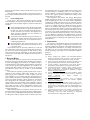
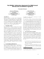
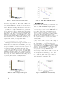
As available sensor node platforms commonly employ dedicated radio transceivers, sensors and peripherals, selectively
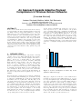
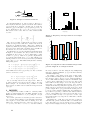
disabling these components allows to measure the node’s energy consumption in diﬀerent conﬁgurations. Exemplarily,
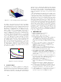
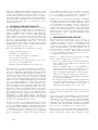
the current consumption ﬁgures for the widely used tmote
sky platform have been taken from the datasheet [9] and
were plotted against each other in Figure 1. It is clearly
visible that the radio transceiver exhibits a power consumption that is about one order of magnitude higher than the
corresponding values for the used microcontroller.
Current [mA]
1.
15
10
5
0
RX / on
TX / on
off / on
off / idle
off/standby
Configuration [Radio/CPU]
Figure 1: Power consumption of tmote sky nodes
(numbers taken from [9])
This paper compares two methods to reduce traﬃc in sensor
networks (see Section 2) and outlines their mode of operation. Special emphasis is put on their applicability in WSNs,
as resource-constrained devices generally exhibit characteristics that diﬀer from common desktop computers. Subsequently, we present our approach towards an adaptive packet
compression framework for sensor network applications in
Section 3. By compressing sensor data with the locally optimal energy eﬃciency ratio, energy can be preserved and thus
the node lifetime extended. The description of our vision is
followed by an analysis of related work. Finally, conclusions
and an outlook will be presented in Section 4.
19
2.
REDUCING TRAFFIC IN THE WSN
Although several methods of reducing the size or number
of packets in WSNs exist, we introduce two common solutions in this section. Data aggregation tries to optimize
the number of transmissions throughout the sensor network,
while data compression strives for a local optimization of the
amount of transmissions and their payload size.
2.1
Data Aggregation
If incoming packets and locally generated data are addressed
to the same destination, combining these data sets into a
single packet can eﬀectively reduce the number of transmissions required [5]. For example, consider the linear topology
depicted in Figure 2. The rightmost node (S) acts as a sink
to sensor readings from the remaining nodes (A, B, C).
gorithms often achieve good average compression ratios on
various types of input data, algorithms adapted to speciﬁc
applications often provide better performance, however at
the cost of being limited to a narrow application area.
A common metric to evaluate the savings achieved by data
compression is the energy cost per bit. Data compression
is only feasible in terms of energy eﬃciency if the computational eﬀorts to reduce the payload size by one bit are lower
than the energy required for transmitting this additional
bit. Depending on the used components, current sensor node
platforms can perform 4.000 to 2.000.000 CPU cycles [8] instead of transmitting a single byte, while still maintaining a
positive energy balance.
3.
VISION
The vision of our research is to develop a modular compression framework, which can be deployed on nodes in a WSN.
It comprises a set of diﬀerent compression and decompression algorithms, which can be adaptively selected, and even
combined to achieve additional savings. By compiling the
algorithms into packages, diﬀerent compression methods can
be dynamically selected, exchanged and updated during runtime.
Figure 2: A linear sensor network topology
If only one-hop connectivity is given, a total of six transmissions are required to forward all measured data to the
sink (depicted as the multi-hop forwarding case). Another
downside of this issue is that node C, located next to the
sink, must forward a higher count of packets than A or B
and will thus most likely deplete its energy budget ﬁrst.
Aggregating the incoming sensor data with local readings
and forwarding these results to the sink can reduce the required number of transmissions from six to three in this basic
scenario, hence achieving savings of 50% in the number of
transmissions. This is indicated in the lower part of Figure 2,
where only a single aggregated data packet is forwarded by
each node.
Although node distributions in real deployments might considerably diﬀer from this example, it should be remarked
that the number of packets cannot increase by applying data
aggregation.
2.2
Data Compression
Opposed to the previously described mechanisms of data
aggregation, data compression targets to locally reduce the
packet payload size by increasing the information density
within a packet. In general, compression algorithms can be
classiﬁed as either lossless or lossy. While some applications
(such as software updates) require a bitwise correct transmission of data, intrinsic oﬀsets in sensor hardware might
reduce the achievable accuracy and thus provide an application area for lossy compression.
A variety of diﬀerent approaches exist, and will be brieﬂy
introduced in Section 3.1. While generic compression al-
20
As many current sensor network applications follow predeﬁned structure deﬁnitions in their output data formatting, diﬀerent compression algorithms will typically produce
diﬀerently sized output. The framework can either rely on
application-deﬁned preferences regarding the preferred compression engine, or compress an exemplary set of sensor data
with its available compressors prior to selecting the algorithm with the highest energy eﬃciency. While this analysis
might consume more energy before regular operation, it only
needs to be performed once and will subsequently use the
locally optimal compression algorithm.
Additionally, applications can also specify delay bounds for
the compression of their packets. This mechanism ensures
that lengthy algorithms are avoided when low latency transmissions are required. The framework is targeted to allow dynamic updates and modiﬁcations of the compressors
and/or compressor parameters during runtime. This allows
to exchange slow implementations of algorithms with optimized ones and tune parameters to fulﬁll the application’s
needs.
3.1
Related Work
A variety of data compression (and decompression, respectively) algorithms are well-known, although only few of them
were speciﬁcally tailored to ﬁt the needs of sensor networks.
The emerging ﬁeld of sensor networks however poses diﬀerent constraints on resulting algorithms than common desktop computers do. Both processing power and available
memory are tightly limited in sensor nodes, and their tight
energy budget must additionally be considered. For these
reasons, heavyweight compressors, such as partial predictive matching (PPM), or similar algorithms that require big
dictionaries to be stored in RAM, cannot be run on the
nodes. The even more sophisticated PAQ compressor quotes
a minimum RAM consumption of 35 megabytes, although
values range up to 1712MB1 . Barr and Asanović performed
an analysis of several compression algorithms on a Compaq
Personal Server handheld device in [2]. The platform featured a 233MHz CPU with 32 megabytes of RAM, rendering a direct mapping of the results to sensor node platforms
equipped with low-power CPUs and a few kilobytes of RAM
impossible.
Other authors have noticed this discrepancy between highly
demanding but eﬃcient compression algorithms and sensor
node capabilites, and have thus designed algorithms specifically adapted to sensor networks, such as S-LZW [8] and
SBZIP [10]. However, Tsiftes et al. have mainly regarded
software updates that were compressed before deployment
in [10]. Software updates are deployed less frequently than
data packets, and even when a higher number of packets are
required to transmit an application image, the necessity to
compress packet payloads still persists.
4.
CONCLUSION
Limited energy budgets of sensor network nodes make data
compression a necessity when energy savings are required.
However, it is very likely that there is no universally optimal
compression algorithm for sensor network data. Instead,
the need to adapt to the payload contents and dynamically
choose the appropriate compression algorithm that yields
best compression rates whilst preserving energy is arising
to keep the energy consumption low and thus enhance node
lifetime.
Compression algorithms implemented for desktop computers
are generally not suited for sensor nodes, as they have high
requirements towards CPU and memory size. However, a
lot of existing approaches and concepts can be applied in
sensors networks in modiﬁed forms. We propose the use of
a modular compression framework that can be dynamically
updated during runtime, while automatically detecting the
locally optimal compression scheme for application-speciﬁc
data.
When data from diﬀerent sources is present in sensor nodes,
generic compression algorithms will not always yield optimum results. In such application scenarios, we expect our
compression framework to outperform solutions that rely on
a single static compressor and thus achieve high energy savings.
5.
[4] P. Dutta, J. Hui, J. Jeong, S. Kim, C. Sharp,
J. Taneja, G. Tolle, K. Whitehouse, and D. Culler.
Trio: Enabling Sustainable and Scalable Outdoor
Wireless Sensor Network Deployments. In Proceedings
of the Fifth International Conference on Information
Processing in Sensor Networks (IPSN), 2006.
[5] C. Intanagonwiwat, R. Govindan, and D. Estrin.
Directed Diﬀusion: A Scalable and Robust
Communication Paradigm for Sensor Networks.
Proceedings of the 6th Annual International
Conference on Mobile Computing and Networking
(MobiCom), 2000.
[6] B. H. Liu, N. Bulusu, H. Pham, and S. Jha. CSMAC:
A Novel DS-CDMA Based MAC Protocol for Wireless
Sensor Networks. In Proceedings of the 2004 IEEE
Global Telecommunications Conference Workshops
(GLOBECOM), 2004.
[7] J. Polastre, J. Hill, and D. Culler. Versatile Low
Power Media Access for Wireless Sensor Networks. In
Proceedings of the 2nd International Conference on
Embedded Networked Sensor Systems (SenSys), 2004.
[8] C. M. Sadler and M. Martonosi. Data Compression
Algorithms for Energy-Constrained Devices in Delay
Tolerant Networks. In Proceedings of the 4th
International Conference on Embedded Networked
Sensor Systems (SenSys), 2006.
[9] Sentilla Corp. Tmote Sky Datasheet. Online:
http://www.sentilla.com/moteiv-endoflife.html,
2007.
[10] N. Tsiftes, A. Dunkels, and T. Voigt. Eﬃcient Sensor
Network Reprogramming through Compression of
Executable Modules. In Proceedings of the 5th Annual
IEEE Communications Society Conference on Sensor,
Mesh and Ad Hoc Communications and Networks
(SECON), 2008.
[11] W. Ye, J. Heidemann, and D. Estrin. An
Energy-Eﬃcient MAC protocol for Wireless Sensor
Networks. Technical Report ISI-TR-543, Information
Science Institute (ISI) / University of Southern
California (USC), 2001.
REFERENCES
[1] I. Akyildiz, W. Su, Y. Sankarasubramaniam, and
E. Cayirci. A Survey on Sensor Networks. IEEE
Communications Magazine, 40:102–114, 2002.
[2] K. Barr and K. Asanović. Energy Aware Lossless Data
Compression. In Proceedings of the First International
Conference on Mobile Systems, Applications, and
Services (MobiSys), 2003.
[3] M. Buettner, G. Yee, E. Anderson, and R. Han.
X-MAC: A Short Preamble MAC Protocol For
Duty-Cycled Wireless Sensor Networks. In Proceedings
of the 4th International Conference on Embedded
Networked Sensor Systems (SenSys), 2006.
1
According to the developer homepage at http://www.cs.
fit.edu/~mmahoney/compression/
21
Connectivity-aware Neighborhood Management Protocol
in Wireless Sensor Networks
Christoph Weyer, Stefan Unterschütz, and Volker Turau
Institute of Telematics
Hamburg University of Technology, Germany
[email protected]
ABSTRACT
Neighborhood relations are changing over time in wireless
sensor networks due to diﬀerent hardware or environmental
eﬀects. These eﬀects and memory limitations require a balanced neighborhood management to ensure agility, stability,
symmetry, and connectivity. The proposed neighborhood
management protocol Mahalle is optimized with regard to
these four criteria. Agility and stability are achieved by
ALE, a new adaptive link estimator.
1.
INTRODUCTION
Many applications or algorithms for wireless sensor networks
depend on a priori knowledge of neighborhood information.
This encompasses information about neighborhood relations,
i.e., which nodes can communicate with each other, and
information about the link quality and reliability between
those nodes. Self-stabilizing algorithms are a prominent example of algorithms that highly depend on neighborhood
information [3]. The quality of neighborhood information
can be described by four criteria: agility, stability, symmetry, and connectivity.
Before accounting a node as a neighbor the quality and reliability of the communication link between the nodes must be
assessed. Many parameters of the environment, e.g., multipath eﬀects, lead to a variation of these link properties over
time. Due to the characteristics of the wireless channel,
neighborhood relations are not known a priori and can only
be gathered after the deployment when the network is in
operation.
The local view upon the neighborhood of a node forms the
topology of the network at the global scope. Variations in
hardware, changes in the environment, or node failures lead
to dynamic changes of the topology. Therefore, neighborhood relations are not ﬁxed during the whole lifetime of the
network. Frequent topology changes lead to a degradation of
the algorithms or applications running on top of the formed
topology. This aspect of the quality of a neighborhood protocol is captured by the concepts of agility and stability.
Agility measures the speed of adapting to desirable events,
such as failure of a node respectively a link or deployment
of a new nodes. Stability is the ability to ignore transient
failures.
Despite variation over time the neighborhood relations must
be consistent between nodes. This requirement is expressed
by the symmetry property. In particular, if node A is in the
neighborhood of B, then node B must also be part of the
neighborhood of node A. Otherwise the resulting topology
is not useable in most cases. Reason for such an asymmetrical neighborhood relation is the existence of diﬀerent link
qualities caused by diﬀerent noise levels due to ﬂuctuations
in hardware accuracy. Another reason lays in the memory
restriction of sensor nodes. Memory restrictions are an important topic in regard to ensuring connectivity. If the density of the network is higher than the number of neighbors
that a node can store, a simple neighborhood protocol can
lead to disconnected network.
Therefore, a neighborhood management must ensure these
four quality criteria. This paper presents Mahalle, a new
neighbor management protocol based on adaptive link estimator. Mahalle optimizes the neighborhood relations according to agility, stability, symmetry, and connectivity.
2.
RELATED WORK
Research has mainly focused on link estimation so far. Link
quality can be assessed by the physical or logical properties. Currently available hardware is providing these physical properties with a high accuracy [2]. The link quality
indicator (LQI) or received signal strength indicator (RSSI)
are determined by the radio transceiver. However, the values of these metrics are highly hardware speciﬁc and must
be calibrated for each hardware setting.
Packet reception rate (PRR) is a widely used logical property indicating the link reliability [5]. PRR is calculated
from the rate of successfully received periodical broadcast
packets. Periodic sending is done by discretizing time into
rounds. In each round every node send its broadcast packet.
Besides an identiﬁer of the sender these packets contain a
sequence number that is used to determine packet loss. In
contrast to the physical properties, PRR is the link reliability experienced by applications, but comes at the extra
eﬀort of periodical broadcasts. The main drawback of all
metrics representing the link behavior is that they exclusively describe a snapshot of the state involving only the
recent past. They can not be used as a reliable estimate of
the near future, which is needed to provide stability.
Taking the considerations above into account estimating the
PRR by evaluating the packet reception rate of periodical
broadcasts is the most appropriate way for a solution independent from hardware and environment. In [4] several link
23
The behavior of EWMA is controlled by the parameter α
ranging from 0 to 1. For α = 0.99 EWMA is called stable
and has a high accuracy with a low mean square error but
with a high crossing time. The metric crossing time is deﬁned by the time the estimator needs after detecting a new
link to come up with a PRR value having an error of at most
�. In the following � is assumed to be 0.05. For α = 0.915
EWMA is called agile. This value leads to a much shorter
crossing time and a smaller reaction time to link changes,
but suﬀers from a high variation with a high mean square
error. In [4] the stable EWMA is preferred to the agile in
order to produce more stable link estimations over time. On
top of such a link estimator in [5] a neighborhood protocol
that is aware of asymmetrical links is described. The realization of this, especially with a neighbor table size of 40
entries, is not further explained.
TinyOS 2.x uses the Link Estimation Exchange Protocol
(LEEP) to estimate link reliability and manage neighborhood information [1]. The Extra Expected number of Transmissions (EETX) is used as a link-quality metric. EETX is
the expected value of a geometrically distribution with the
probability PRR not counting the successful transmission.
Therefore, EETX is deﬁned as EETX = (1/PRR) − 1. The
bidirectional EETX value is based on the product of inbound
and outbound packet reception rate that are discrete recursively estimated. Inbound PRR is estimated as the reception
rate at node A by receiving packets from node B. The reception rate from node A at node B is the outbound PRR of
node A. The neighborhood table size is limited to 10 neighbors in TinyOS. To share the outbound quality information
the complete neighborhood table must be exchanged. If the
complete link information does not ﬁt into one packet, a
round-robin schedule is established. If the neighborhood table is full and a new node is detected, the neighbor with a
low EETX value if existent is evicted. This policy is simple,
but can lead to disconnected topologies in dense networks.
3.
ADAPTIVE LINK ESTIMATOR
Since the proposed adaptive link reliability estimator can
be used independently from the neighborhood management
protocol, it is speciﬁed separately in this section. As described in [4] the PRR is estimated by observing the successful delivery of periodical broadcast packets. If applicationspeciﬁc packet rate is suﬃcient, the estimator information
can be sent piggybacked in the data packets in order to reduce the periodical broadcast packets. EWMA in agile mode
is a fast responding link estimator while in stable mode a low
mean square error is achieved. The main goal of the adaptive link estimator proposed in this paper is to combine the
strength of both modes.
The adaptive link estimator (ALE) uses EWMA as a basis.
It has the capability to adjust the parameter α depending on
24
300
crossing time [rounds]
estimation methods are evaluated and compared. The exponentially weighted moving average (EWMA) is one of the
most appropriate methods related to fast response, mean
error and memory usage. PRR is estimated by PRR ←
PRR · α + (1 − α) if a packet was successfully received, and
PRR ← PRR · α if a packet loss occurs. A single or consecutive packet loss is detected by a timeout or on the basis of
sequence numbers.
250
Agile EWMA
Stable EWMA
ALE
200
150
100
50
0
0.1
0.2
0.3
0.4
0.5
0.6
PRR
0.7
0.8
0.9
1
Figure 1: Crossing Time
the current estimated link quality. To improve the crossing
time the initial PRR is set to the threshold value PRRbad ,
whenever the ﬁrst packet is received from a node. In this paper PRRbad is set to 0.5. Additionally, when the PRR is below PRRbad or a new link must be estimated the agile mode
is used in order to estimate quickly the real link quality.
ALE switches from agile into stable mode after 30 rounds
in case that the PRR is greater than PRRbad during this
period for a more accurate estimation. This mechanism is
called raising mechanism, which improves the crossing time
of ALE compared to EWMA. In Figure 1 the crossing time
of the diﬀerent estimators is compared. The crossing time of
the stable EWMA is very high compared to the agile mode.
Due to the threshold PRRbad and the raising mechanism the
crossing time of ALE is even faster than the agile EWMA,
especially for good links. Observe that the crossing time
of ALE is smaller than 30 for all high values of PRR. This
justiﬁes the choice made above for the number of rounds to
switch from the agile to stable mode.
Another mechanism that improves ALE is the so called dropping mechanism. With this mechanism a good link is trusted
even if currently no communication is possible. Doing so
the stability of the resulting network topology is increased.
Whenever a good link, with PRR > PRRgood suﬀers from
consecutive packet loss, the PRR is kept constant for 60
rounds. This number is a parameter of ALE and speciﬁes
the time that is conceded to a node to recover from a transient failure.
In Figure 2 the behavior of EWMA and ALE is compared
over time. As shown in both ﬁgures, ALE outperforms the
agile mode of EWMA in terms of mean square error. Figure 2 (a) shows a link with a ﬁxed real PRR of 0.89 and
a short link interruption of 50 packets in round 1000. This
ﬁgure depicts the improvements during startup of ALE and
especially during the short interruption compared to stable
EWMA. Figure 2 (b) shows a link with a PRR of 0.89, which
is dropping during round 600 and 900 to a PRR of 0.4 and is
interrupted during round 1200 and 1500. Here the improvements introduced by the dropping mechanism are depicted.
If the PRR is dropping below PRRbad the estimation mode
of ALE switches back to the agile mode in order to react
faster on link changes.
1
0.9
0.8
0.8
0.7
0.7
0.6
0.6
PRR
PRR
1
0.9
0.5
0.5
0.4
0.4
0.3
0.3
0.2
0
0.2
Agile EWMA
Stable EWMA
ALE
0.1
0
200
400
600
Agile EWMA
Stable EWMA
ALE
0.1
800 1000 1200 1400 1600 1800 2000
round
(a) Real PRR = 0.89 and short message lost
0
0
200
400
600
800 1000 1200 1400 1600 1800 2000
round
(b) Variation of PRR over time
Figure 2: Comparison between EWMA and ALE
Normally a link is considered as a neighbor if the link quality
is above a given threshold, here deﬁned by PRRgood and
is often set to 0.8. In contrast, a neighbor is disregarded
if its quality drops below PRRgood . Doing so oscillation
eﬀects can occur. Therefore, a hysteresis is used to decrease
oscillation eﬀects as much as possible. Several simulations
revealed that a range of ±0.06 is a good choice between
oscillation and size of the hysteresis. This leads to PRRin =
0.86 and PRRout = 0.74.
4.
NEIGHBORHOOD MANAGEMENT
The neighborhood management protocol Mahalle uses the
information about link qualities between nodes provided by
the adaptive link estimator described in the previous section. ALE delivers only information about one direction of
a communication link. If node A receives packets from node
B it can calculate the PRR of node B at node A by using
ALE. But this information is of no signiﬁcance for the PRR
of node A at node B. To ensure symmetry of the communication links between neighbors the PRR values of both
directions of the link must be exchanged.
The PRR is normally exchanged between nearby nodes by
using periodical broadcasts. In general, three diﬀerent approaches exist. The simplest way is to put the estimated
PRR values of all known nodes in each packet. The main
drawback of this approach is the required size of such a
packet. Due to the high bit error rate, the probability of
packet loss is increased, which inﬂuences the PRR estimation. The second approach is to send only the PRR values
that have changed lately. This decreases the amount of information sent in one packet, but the size varies. If a packet
gets lost, the information must be resent even if the PRR
is unchanged. The complexity of this approach is thereby
increased. Another approach is to send only fractions of the
PRR values in a round-robin schedule. Doing so, all packets
are equally sized and every PRR value is broadcasted with a
ﬁxed schedule. Mahalle uses the last approach to exchange
link information between neighboring nodes. One additional
beneﬁt of this is that additional information can be included
into the broadcast packets, e.g., the node state needed by
self-stabilizing algorithms [3].
The node table consists of entries to store the neighbor list
and the preparation list. The neighbor list contains the
nodes that are treated as neighbors. All other entries in
the node table are used by the preparation list, where potential neighbors are stored in order to be able to estimate
their link quality. At startup the whole node table is occupied by the preparation list. If a node is evicted from the
node table, it is inserted into a blacklist for some time in
order to prevent them to reenter immediately. The number of entries in the node table (Nt ) and the ratio between
the maximum number of entries in the neighbor list (Nn )
and the preparation list (Np ) are compile-time parameters
of Mahalle and correlate to the expected average network
density.
In every round each node broadcasts a neighborhood packet.
This packet contains the identiﬁer of the node, a sequence
number, and one entry of the node table. This information
contains of the identiﬁer of the neighbor and the estimated
PRR. The round-robin schedule consists of Nt rounds, so
that each entry of the node table is rebroadcasted in every
Nt ’th round. This information is used by the nodes that are
receiving the packets.
Node table entries contain of the following information: a
ﬂag that indicates if the node is in the neighbor list, estimated inbound PRR, the received outbound PRR, the number of neighbors and overlapping neighbors, a ﬂag indicating
symmetry, and the age of the entry. Whenever a node receives a broadcast from a node that is contained in its node
table, the corresponding entry is updated. Each packet is
used to estimate the inbound PRR. When the packet contains the identiﬁer of the receiving node, the outbound PRR
in the packet is stored in the table. From all packets during
Nt rounds the node can also identify the number of neighbors of the sending node and the number of overlapping
neighbors, the nodes that are common for both.
When a packet is received by an unknown node and the node
table has a free entry, the node is inserted into the preparation list (if the node table is full the packet is ignored). If
the estimated PRR of the inserted node is above PRRin the
25
Rule 1: Select asymmetry links
Rule 2: Select nodes with neighbors
Rule 3: Select highest overlapping
Rule 4: Select less unknown neighbors
Rule 5: Select lowest bidirectional PRR
Rule 6: Select newest neighbors
The ﬁrst rule tries to evict nodes that are asymmetric from
the list. If several nodes are found or none of the entries
are asymmetrical, the next rule is applied. This rule protects those nodes from being removed that have no other
neighbor. The next rule selects those nodes that have the
highest number of overlapping neighbors, since those nodes
are connected via one of the common neighbors with a high
probability. If there are still several nodes having the same
properties those nodes are selected, which provide the smallest number of unknown neighbors. Those nodes are not that
important for insuring connectivity. These last two rules are
protected by a hysteresis in order to prevent an oscillation effect. In rule 5 the nodes with the lowest bidirectional PRR
are selected to be removed from the neighbor table. This
PRR is the product of the estimated inbound and received
outbound PRR. If still more than one node is selected the
newest neighbors are preferred, since the older neighbors insure more stability. If still several nodes are in the list after
applying the last rule, a node is picked randomly.
The ns-2 simulator is used for validating Mahalle. To compare the connectivity awareness of Mahalle a simple neighborhood management protocol is also implemented, which
uses only the inbound and outbound PRR values provided
by ALE. Additional the LEEP [1] protocol integrated in
TinyOS 2.x (see Section 2) is ported to ns-2. Several different densities with 200 randomly placed nodes are investigated. For each density 50 diﬀerent topologies are used.
The used propagation model provides around 15% of asymmetrical links, which means that the inbound and outbound
PRR diﬀers more than 0.15. In Figure 3 the results for a
density of 24 is shown. 180 Nodes are started at round 0 and
20 nodes where added after 1750 rounds. The connectivity
26
3
2.5
2
75
1.5
50
1
25
0
0.5
0
500
number of link changes
If the neighbor list is full and in the preparation list a link
with PRR > 0.86 exists an entry from the neighbor list must
be evicted to provide space for the new potential neighbor.
Therefore, a screening process exists to choose the most appropriate neighbor that is evicted from the neighbor list.
The following rules are applied to the list containing all
neighbors and the candidates from the preparation list. The
rules are processed one-by-one until a single node remains.
If the new potential neighbor is selected the neighbor list is
kept unchanged and the node is inserted in the blacklist and
removed from the preparation list.
Basic
LEEP
Mahalle
100
connectivity [%]
node is a candidate to be placed into the neighbor list. If
the node stays longer than 50 rounds in the preparation list
without entering the neighbor list, the node is deleted from
the preparation list and added to the blacklist. If a node is
in the neighbor list and its PRR is below PRRout the node
is removed from the list and added to the blacklist.
0
1000 1500 2000 2500 3000 3500 4000
time [rounds]
Figure 3: Comparison with network density 24
and the number of link changes are shown over time. Mahalle provides very fast neighborhood detection and reaches
100% connectivity. Due to the large density of 24 potential neighbors, LEEP and the basic protocol are providing
only a slow convergence. Connectivity is not fully reached
by these two approaches after adding nodes. The number
of link changes during the stable phases is also decreased in
Mahalle.
5.
CONCLUSION
The presented neighborhood management protocol Mahalle
and the underlying adaptive link estimator have shown good
results in terms of agility, stability, symmetry, and stability.
Mahalle outperforms in terms of stabilization speed. The
next steps will be porting Mahalle to TinyOS and using it
in a real long-term deployment at our campus.
6.
ACKNOWLEDGEMENT
We would like to thank Ting-Fu Chen for his help in developing a preliminary version of Mahalle.
7.
REFERENCES
[1] O. Gnawali. TinyOS Extension Proposal (TEP) 124:
The Link Estimation Exchange Protocol (LEEP), Feb.
2007.
http://www.tinyos.net/tinyos-2.x/doc/pdf/tep124.pdf.
[2] K. Srinivasan and P. Levis. RSSI is Under Appreciated.
In Proceedings of the Third Workshop on Embedded
Networked Sensors (EmNets’06), Harvard University
Cambridge, MA, USA, May 2006.
[3] V. Turau and C. Weyer. Randomized Self-stabilizing
Algorithms for Wireless Sensor. In Proceedings of the
International Workshop on Self-Organizing Systems
(IWSOS’06), Passau, Germany, Sept. 2006.
[4] A. Woo and D. Culler. Evaluation of Eﬃcient Link
Reliability Estimators for Low-Power Wireless
Networks. Technical Report UCB/CSD-03-1270, U.C.
Berkeley Computer Science Division, Sept. 2003.
[5] A. Woo, T. Tong, and D. Culler. Taming the
Underlying Challenges of Reliable Multihop Routing in
Sensor Networks. In Proceedings of the First ACM
Conference on Embedded Networked Sensor Systems
(SenSys’03), Los Angeles, CA, USA, Nov. 2003.
Challenges in Short-term Wireless Link Quality Estimation
Alexander Becher
Muhammad Hamad Alizai, Olaf Landsiedel,
Klaus Wehrle
sd&m AG
Düsseldorf, Germany
Distributed Systems Group
RWTH Aachen University, Germany
[email protected]
ﬁrstname.lastname @rwth-aachen.de
Abstract
Identifying reliable low-power wireless links for packet
forwarding in sensor networks is a challenging task. Currently, link estimators mainly focus on identifying highquality stable links, leaving out a potentially large set of
intermediate quality links capable of enhancing routing
progress in a multihop network.
In this paper we present our ongoing work on short-term
link estimation that captures link dynamics at high resolution in time. A short-term link quality is calculated based on
the recent transmission characteristics of a link. This shortterm quality of a link, combined with its long term reliability
enables to determine if an intermediate quality link is temporarily available for transmission. Consequently adapting
the neighbor table of a node and offering more forwarding
choices to routing protocols.
1
Introduction
Instability in low-power wireless sensor networks (WSN)
connectivity has so far been regarded as a difﬁcult problem
that existing routing algorithms try their utmost to avoid. In
doing so, they forego a large class of potentially valuable
communication links. An understanding of the patterns underlying the seemingly irregular variations of the wireless
channel would enable algorithms to make use of this previously disregarded class of links.
To achieve better connectivity and reliable packet communication, today’s link estimators restrict communications
only to the neighbors with constantly high-quality links.
These high quality links are identiﬁed based on the long
term success rate of a link, typically collected over a time
frame on the order of minutes. However, this approach has
certain pitfalls. First, neighbors with intermittent connectivity might reach farther into the network. Their use would
therefore reduce the number of hops, reduce energy usage
in the network, and increase its lifetime. Second, in a sparse
network with a low density of nodes, a node might have no
high-quality neighbor in its communication range, requiring
a mechanism to deal with unstable connectivity.
In this paper we present our on going work on short-term
link estimation (STLE) [2] that takes ﬁne-grained link dynamics - in the order of milliseconds - into account and increases the prediction quality for successful packet transmissions, especially, for highly dynamic links. STLE integrates
into routing protocols by adapting neighbor tables to accu-
rately reﬂect the current situation of a dynamic link. Overall,
short-term link estimation has three key contributions: (1) to
predict the probability of successful packet transmission of
any link type by taking short-term dynamics into account,
(2) to suggest links of low to intermediate quality for routing when they have become temporarily reliable, and (3) to
integrate easily with today’s long-term link estimators and
routing protocols.
2
Related Work
The identiﬁcation of reliable links in WSN has received
much attention in the recent years. However, to the best of
our knowledge, there is no thorough analysis of short-term
dynamics in link quality. This paper aims to ﬁll this gap by
quantifying their extent and characteristics.
While investigating several approaches for online link
estimation, Woo et al. [20] identiﬁed window mean estimator with an exponentially weighted moving average
(WMEWMA) to be an optimal choice to aggregate packet
reception rate as an indicator of link quality. Four-bit link
estimation [6] extends this WMEWMA estimator into a hybrid link estimator that accumulates information from all
layers of the sensor node networking stack. However, estimation techniques based on WMEWMA performs poorly
on medium quality links. These links often offer the highest routing progress [3] suggesting the need for more precise
estimation methods for medium quality links.
The assumption underlying the majority of existing link
estimation concepts is that packet losses inside one measurement period occur independently of each other (i. e., they follow a Bernoulli distribution). This assumption has been challenged before in research [4, 14]. The analysis of our data in
Section 4 supports the hypothesis that the assumption of independent packet losses is not appropriate at the ﬁne-grained
time-scales dealt with in this paper.
In addition to online link estimators, there has been significant research in link modelling and link measurements for
WSN [1,13,15–17,21–23]. For example, Koksal et al. [9] develop metrics to model long-term link quality and short-term
link dynamics. Additionally, Cerpa et al. [3] provide statistical models of radio links in WSN, including short-term and
long-term temporal characteristics.In contrast to these approaches, STLE does not aim to provide link models, but to
identify phases of reliable or unreliable connectivity at runtime.
27
1
0.8
Good links (quality > 0.9)
0.8
Intermediate links
Probability
CDF
0.6
(0.1 < quality < 0.9)
0.4
Bad links (quality < 0.1)
0.2
0
0
0.1
0.2
0.3
0.4
0.5
0.45
quality > 0.9
quality > 0.1
Temporal Standard Deviation
1
0.6
0.4
0.2
0.6
0.7
0.8
0.9
1
0
2
4
6
8
Long-Term Link Quality
10
12
14
Distance (metres)
16
18
20
0.4
0.35
0.3
0.25
0.2
0.15
0.1
0.05
0
0
0.1
0.2
0.3
0.4
0.5
0.6
0.7
0.8
0.9
1
Long-Term Link Quality
(a) Empirical distribution of long-term link qual- (b) Probability of ﬁnding a high-quality or (c) Temporal variation of link quality. Each point
ity in our testbed. Intermediate quality links com- medium-to-high-quality neighbor depending on represents a (directional) node pair.
prise roughly one third of all useful links.
physical distance in our testbed.
Figure 1. Low-power radio links in sensor networks exhibit inevitable ﬂuctuations in their quality.
Approaches such as Solicitation-based forwarding (SOFA
[10]) remove the need for long-term link estimation and test
link availability by sending a short hand-shake packet as a
probe before sending any data packets. However, our evaluation of STLE in Section 4 shows that a successful hand-shake
should not be taken as a success guarantee for subsequent
data transmissions and indicate a need for more sophisticated
models.
3
Short-term Link Estimation
In this section we introduce short-term link estimation in
detail, putting a special focus on its integration into longterm link estimators and routing protocols. We present our
approaches on the identiﬁcation of temporarily available and
unavailable links and evaluate these in Section 4. Our interest in short-term link estimation is motivated by two key observations indicated by research [3,13,21] and our own measurements: (1) Links of intermediate quality amount to about
half the number of high-quality stable links (see Figure 1(a))
and (2) this percentage grows with the physical distance (see
Figure 1(b)).
Although links of intermediate quality offer further
choices for routing and often promise long distance connectivity, Figure 1(c) shows that this class of links is subject to large and frequent temporal variations. Their dynamic
connectivity poses a special challenge to any link estimator.
Long-term link estimators are not designed to identify shortterm link dynamics. As a result, they adapt slowly to changing link conditions, limiting their use to the identiﬁcation of
long-term stable links.
3.1
Deriving a Short-term Link Estimator
Commonly, links in a wireless network can be classiﬁed
into three categories: good links that are reliable in the long
term; intermediate, unreliable links often with frequently
changing quality; and bad links that very seldom transmit a
packet successfully. Figure 1(a) shows that the ratio between
good links and intermediate links is 2:1 in our testbed measurements. Furthermore, our measurements indicate that any
link – no matter of what long-term quality – can temporarily
change its characteristics and thereby temporarily become a
reliable link for routing or become an unreliable one.
We consider an intermediate or broken link temporarily
available when it successfully transmits a number of pack-
28
ets over a short interval. We deﬁne a corresponding threshold based on the link’s long-term reliability: for example,
a link of intermediate quality needs to transmit less packets before being considered temporarily available than a link
of bad quality. Similarly, a number of successfully transmitted packets indicate that a reliable link is currently available,
while failed ones indicate that a link is currently not available. Overall, we expect that a single successful transmission
indicates that a long-term reliable link is currently available.
Furthermore, short-term link estimator does not send
probe packets to test for link availability, it bases on packet
overhearing. Hence, a node overhears packets sent by neighboring nodes and collects statistics on the current reachability. When a node considers the incoming direction of an unreliable link temporarily stable and concludes that it offers a
routing improvement, it sends a message to the link neighbor
to inform it about a short-term link availability. The neighboring node may then consider routing subsequent packets
over the newly available link. If the node is selected as next
hop, link-layer acknowledgments continuously provide information about link availability.
We expect that the probability of a successful packet
transmission depends on the success rate of any recently sent
packets, i.e. the more packets were transmitted successfully
in the recent history, the higher the probability is that an upcoming packet is transmitted successfully, too.
3.2
Integration with Long-Term Link Estimators and Routing Protocols
STLE is designed to embed deeply into the routing protocol and to cooperate with long-term link estimators. Modern
sensor network routing protocols such as BVR [7] use the
number of expected transmissions to a destination as routing metric, computed by combining the distance (in hops)
and the number of expected retransmissions. Both long-term
and short-term link estimation aim to predict the number of
necessary retransmissions on a link, each on their respective
temporal granularity. Consequently, when no short-term estimation for a link is available, the routing protocol will use
the long-term prediction as fallback, probably resulting in
conservative link selection.
As explained above, neighboring nodes overhear ongoing data ﬂows and may suggest themselves to the forward-
0.8
0.7
Short-Term Link Quality
Short-Term Link Quality
1
0.9
0.8
0.7
0.6
0.5
0.4
0.3
0.2
0.1
0
1
0.8
0.6
0.4
0.8
0.6
0.4
0.2
0.2
0
0
1
0.8
0.6
0.4
Long-Term Link Quality
0.2
0 0
1
0.9
0.8
0.7
0.6
0.5
0.4
0.3
0.2
0.1
0
1
1
0.8
5 6
5/6 4
4/5 3
3/4
2
Success History
1 2/3
0.6
0.4
Long-Term Link Quality
0.2
0 0
1
2/3
2
3/4
3
4/5
4
5/6
5
6
Failure History
(a) Inﬂuence of recent transmission success rate on short-term link quality. (b) Inﬂuence of recent transmission failure rate on short-term link quality.
A label of k/h stands for k successes during the last h transmissions, and h A label of k/h stands for k failures during the last h transmissions, and h is
is a shorthand for h/h.
a shorthand for h/h.
Figure 2. Inﬂuence of success and failure of recent transmissions events on short-term link quality.
ing node as next hop alternatives, when they (1) identify the
link from the forwarding node as short-term reliable and (2)
conclude that they offer a better routing choice for the ongoing ﬂow. As a result, the forwarding node has an increased
number of choices for routing. Apart from the number of expected transmissions to a destination as used in BVR, other
routing metrics such as link load, queue length or battery levels can be integrated similarly.
3.3
Use Case for STLE
Packet overhearing technique employed in STLE can beneﬁt from the bursty trafﬁc patterns observed in WSN. Typical
applications [8, 11, 18, 19] of WSN involve monitoring environment for events that are of interest to the users. Although
these events occur rarely, but their occurrence results in large
bursts of packets that represent major fraction of the overall
network trafﬁc. In such situations, STLE, after overhearing
ﬁrst few packets, can identify intermediate quality links temporarily available for transmission.
For example, consider a sensor network based fence monitoring system [19]. During normal conditions, i.e. when
there is no intruder breaking into the fence, the network will
generate very limited or no trafﬁc. However, as soon as an intruder is detected by the system, large bursts of packets will
be generated by the distributed event detection algorithm.
In this situation, STLE recognizes intermediate quality links
currently stable for transmission, and informs routing algorithm of the availability of such links by online adaptation of
neighbor tables. We believe that this technique will signiﬁcantly reduce the hop count a packet has to traverse from its
source to destination. Thereby minimizing the energy consumption and increasing network life time.
4
Evaluation
To evaluate the concept of short-term link estimation, we
executed a number of experiments in our indoor testbed. The
testbed consists of a regular 6 × 6 grid of Telos B motes [12]
with a spacing of approximately 2.80 m inside a 20 m × 20 m
indoor auditorium. Every node transmitted a burst of 20 sequentially numbered packets with a length of 15 bytes at 25 dBm. We ran this experiment for 5,500 seconds.
To calibrate STLE we need to identify a threshold when
an intermediate or bad link should be considered temporary
reliable. Figure 2(a) depicts the probability of a successful packet transmission based on the average long-term link
quality and a short-term history of consecutively transmitted
packets. The ﬁgure indicates that e. g. for a link with 10 %
long-term link quality, the transmission success probability
for the next packet exceeds 80% when the four preceding
packets were transmitted successfully. We consider links of
such instantaneous quality useful for routing, thus STLE suggests such a 10 %-quality link for routing. In the same way,
STLE considers a 60 %-quality link to be short-term reliable
after just one successful transmission.
Figure 2(b) depicts the probability of a successful packet
transmission based on the average long-term link quality and
a short-term history of consecutively failed packet transmissions. It indicates that for two or more consecutive losses
any link should be temporarily considered broken and be removed from the routing table.
5
Future Work and Challenges
Although our evaluation shows that STLE can reliably
identify when unstable links have become temporary stable
and vice versa, only an integration can fully evaluate the beneﬁts of STLE. Thus, we are currently implementing STLE
extensions to the link estimator in the Beacon Vector Routing (BVR) protocol to analyze performance improvements
of STLE.
Cerpa et al. [5] discuss the impact of packet size on packet
reception rate. In our experiment, all packets sent were of the
same length. The effect of different packet sizes on packet
reception rate remains to be investigated.
In practice, nodes do not transmit at the same short intervals used during our measurements. We have yet to investigate whether the correlations derived in section 4 hold
29
for longer intervals between reception events. Devising other
mechanisms, such as sending probe packets to evaluate link
quality, could also be used but it will raise the communication overhead signiﬁcantly.
6
Conclusion
Intermediate quality links constitute a signiﬁcant fraction of wireless links in low-power WSN. STLE captures
short-term link dynamics of these links at a high resolution
in time and predicts their temporary availability or unavailability. Our measurements indicate that these intermittent
links, if utilized, can signiﬁcantly improve the performance
of routing algorithms by offering further choices for forwarding packets. Moreover, STLE is more suitable for networks
showing bursty trafﬁc patterns such as in typical applications
of WSN.
7
References
[1] G. Anastasi, M. Conti, E. Gregori, A. Falchi, and A. Passarella. Performance Measurements of Mote Sensor Networks. In 7th ACM International Symposium on Modeling, Analysis and Simulation of Wireless
and Mobile Systems (MSWiM), Venice, Italy, October 2004.
[2] A. Becher, O. Landsiedel, G. Kunz, and K. Wehrle. Towards shortterm link quality estimation. In Proc. of The Fith workshop on Embedded Networked Sensors (Emnets 2008), June 2008.
[3] A. Cerpa, J. L. Wong, L. Kuang, M. Potkonjak, and D. Estrin. Statistical model of lossy links in wireless sensor networks. In Proc. of
the 4th International Symposium on Information processing in Sensor
Networks (IPSN), April 2005.
[4] A. Cerpa, J. L. Wong, M. Potkonjak, and D. Estrin. Temporal properties of low power wireless links: Modeling and implications on multihop routing. In Proc. of the 6th ACM Interational Symposium on Mobile Ad Hoc Networking and Computing (MobiHoc), May 2005.
[5] A. Cerpa, J. L. Wong, M. Potkonjak, and D. Estrin. Temporal properties of low power wireless links: modeling and implications on multihop routing. In MobiHoc ’05: Proceedings of the 6th ACM international symposium on Mobile ad hoc networking and computing, 2005.
[6] R. Fonseca, O. Gnawali, K. Jamieson, and P. Levis. Four-bit wireless link estimation. In Proc. of the Sixth Workshop on Hot Topics in
Networks (HotNets), November 2007.
[7] R. Fonseca, S. Ratnasamy, J. Zhao, C. T. Ee, D. E. Culler, S. Shenker,
and I. Stoica. Beacon vector routing: Scalable point-to-point routing in
wireless sensornets. In 2nd Symposium on Networked Systems Design
and Implementation (NSDI), May 2005.
[8] T. He, S. Krishnamurthy, J. A. Stankovic, T. Abdelzaher, L. Luo,
R. Stoleru, T. Yan, L. Gu, J. Hui, and B. Krogh. Energy-efﬁcient
surveillance system using wireless sensor networks. In MobiSys ’04:
Proc. of the 2nd international conference on Mobile systems, applications, and services, 2004.
[9] C. E. Koksal and H. Balakrishnan. Quality-aware routing metrics for
time-varying wireless mesh networks. IEEE Journal on Selected Areas in Communications, 24(11):1984–1994, November 2006.
30
[10] S.-B. Lee, K. J. Kwak, and A. T. Campbell. Solicitation-based forwarding for sensor networks. In Proc. of the Conference on Sensor and
Ad Hoc Communications and Networks (SECON), September 2006.
[11] K. Lorincz and M. Welsh. A robust, decentralized approach to rf-based
location tracking. Technical report, Harvard University, 2004.
[12] J. Polastre, R. Szewczyk, and D. Culler. Telos: enabling ultra-low
power wireless research. In Proc. of the Fourth International Symposium on Information Processing in Sensor Networks (IPSN), 2003.
[13] N. Reijers, G. Halkes, and K. Langendoen. Link layer measurements
in sensor networks. In 1st IEEE Int. Conf. on Mobile Ad-hoc and
Sensor Systems, October 2004.
[14] K. Srinivasan, P. Dutta, A. Tavakoli, and P. Levis. Understanding the
causes of packet delivery success and failure in dense wireless sensor networks. In Proceedings of the 4th International Conference on
Embedded Networked Sensor Systems (SenSys), November 2006.
[15] P. von Rickenbach, S. Schmid, R. Wattenhofer, and A. Zollinger. A
robust interference model for wireless ad-hoc networks. In 5th International Workshop on Algorithms for Wireless, Mobile, Ad Hoc and
Sensor Networks (WMAN), April 2005.
[16] P. Wang and T. Wang. Adaptive routing for sensor networks using
reinforcement learning. In Proc. of the Sixth IEEE International Conference on Computer and Information Technology (CIT), 2006.
[17] Y. Wang, M. Martonosi, and L.-S. Peh. A supervised learning approach for routing optimizations in wireless sensor networks. In Proc.
of the 2nd International Workshop on Multi-hop Ad-hoc Networks:
from Theory to Reality (REALMAN), 2006.
[18] M. Welsh, G. Werner-Allen, K. Lorincz, O. Marcillo, J. Johnson,
M. Ruiz, and J. Lees. Sensor networks for high-resolution monitoring of volcanic activity. In SOSP ’05: Proc. of the twentieth ACM
symposium on Operating systems principles, 2005.
[19] G. Wittenburg, K. Terﬂoth, F. L. Villafuerte, T. Naumowicz, H. Ritter,
and J. H. Schiller. Fence monitoring - experimental evaluation of a
use case for wireless sensor networks. In In Proc. of 4th European
Conference on Wirless Sensor Networks EWSN, 2007.
[20] A. Woo, T. Tong, and D. Culler. Taming the underlying challenges of
reliable multihop routing in sensor networks. In Proc. of the 1st International Conference on Embedded Networked Sensor Systems (SenSys), November 2003.
[21] J. Zhao and R. Govindan. Understanding packet delivery performance in dense wireless sensor networks. In Proc. of the 1st International Conference on Embedded Networked Sensor Systems (SenSys),
November 2003.
[22] G. Zhou, T. He, S. Krishnamurthy, and J. A. Stankovic. Impact of
radio irregularity on wireless sensor networks. In Proc. of the Second International Conference on Mobile Systems, Applications, and
Services (MobiSys 2004), June 2004.
[23] M. Zuniga and B. Krishnamachari. Analyzing the transitional region
in low power wireless links. In Proc. of the Conference on Sensor and
Ad Hoc Communications and Networks (SECON), 2004.
SomSeD: An Interdisciplinary Approach for Developing
Wireless Sensor Networks
1
2
1
2
Sebastian Georgi , Christoph Weyer , Martin Stemick , Christian Renner ,
3
4
5
5
6
Felix Hackbarth , Ulf Pilz , Jens Eichmann , Tobias Pilsak , Harald Sauff ,
7
8
9
Luis Torres , Klaus Dembowski , Fabian Wagner
Hamburg University of Technology
[email protected], [email protected]
ABSTRACT
The research ﬁeld ”Self organized mobile Sensor and Datanetworks” (SomSeD) is introduced. Its purpose is the investigation of Wireless Sensor Networks (WSN). It beneﬁts
from interdisciplinary exchange between various institutes
of the Hamburg University of Technology (TUHH). Due to
diﬀerent design constraints (such as energy-eﬃciency and
package size) compared to well known classical computer
networks, all aspects of the development of WSNs must be
reconsidered. This paper describes the advantage of having
experts of various faculties both in computer science and
electrical engineering in a single research ﬁeld. In addition
to the introduction of the participating institutes, the deployment of a WSN on the TUHH campus will be outlined.
1.
SOMSED
Since the foundation of the Hamburg University of Technology a unique organization structure has been applied. On
the one hand teaching is distinguished in classical deaneries.
Research on the other hand is performed over boundaries
of faculties in distinct research ﬁelds. Thus, teaching and
research are related to each other in a matrix organization
structure.
One of these research ﬁelds is ”Self organized mobile Sensor
and Data networks” (SomSeD). Its beneﬁts, goals and challenges will be described in this paper. Besides the coordination on the level of the university teachers, the cooperation
of undergraduate and Ph.D students is encouraged. Within
SomSeD the so called ”Junior” group has been created, in
which Ph.D candidates design and develop a WSN. The degree of freedom is high, all decisions regarding the system
design are made by the participants themselves. Thus the
1Institute
2Institute
3Institute
4Institute
5Institute
6Institute
7Institute
8Institute
9Institute
of Telecommunications
of Telematics
of Automation
of Control Systems
of Measurement Technology
for Security in Distributed Applications
of Communication Networks
of Microsystem Technology
of Nanoelectronics
launch of SomSeD-Junior leads to a great motivation and
an appreciable progress.
Deploying a WSN for long-term measurements is one objective of SomSeD. This network is intended to be a platform
to integrate all results from research. The TUHH campus
is well suited to sustain a WSN due to its continuous area.
A permanent installation will support practical demonstrations for various applications and technological concepts of
WSNs. This encourages the interest in SomSeD.
2.
INSTITUTE COOPERATION
Developing WSNs demands contributions from all experts
in the ﬁeld of electrical engineering and computer science,
because all components in both hardware and software have
to be aligned to each other. While Quality of Service criteria such as goodput and latency of classical networks can
be loosened, energy-eﬃciency, reliability in adverse conditions, low complexity and the size of single sensor nodes are
the most important challenges. Classical models such as
the OSI-reference model are given up to allow a crosslayer
design: The application has a very strong inﬂuence on all
layers of abstraction, e.g., routing and media access control
(MAC) must be considered together when energy-eﬃciency
shall be achieved [2].
To fulﬁll these demands, a strong cooperation between different faculties is necessary to deﬁne interfaces and redesign
all components. Although the individual nodes are very
small, the overall complexity of WSNs and the bandwidth of
research topics is still high; beginning with hardware aspects
such as sensor design and autonomous energy supply and
reaching to software methods like data-gathering and visualization. The following institutes participating in SomSeD
represent a unique aggregation of competence in WSN development.
The Institute of Telematics has been active in research of
WSNs since 2004 [3]. It is obvious, that Telematics is the
best choice to supervise the research ﬁeld and to build the
bridge between communication and information engineers.
The Institute of Telecommunications has its traditional research activities in radar development and broadband communications. While the radar technique already performed
31
Security
Visualization
Automation
Routing
Telematics
Application
Communication
Networks
Medium Access
Control Systems
Power
Telecommunication
Radio
Microsystems
Technology
Sensors
Integration
Nanoelectronics
Measurement
Technology
Task
Institute
Figure 1: Hardware Overview
the transformation from large rotating antennas with huge
transmit power into small and cheap automotive equipment,
the communications section is also gaining more and more
interest in wireless sensor networks.
Sensors are a major component of WSNs. Hence, it is natural to include the Institute of Measurement Technology into
the research ﬁeld. Besides a profound knowledge about various sensors, the Institute oﬀers a great experience in ﬁeld
testing.
Another crucial point is Networking. The Institute of Communication Networks plays an important role in developing
suitable routing and networking algorithms. Careful design
of these algorithms helps to decrease protocol overhead and
retransmissions and thus improves energy-eﬃciency.
Cheap and small sensor nodes can only be realized, if a high
integration can be achieved. The Institute of Nanoelectronics oﬀers the complete competence in the design of integrated
circuits in up-to-date process technology.
The Institute of Microsystem Technology is capable of building very complex and sensitive sensors with small size. A focus lies on the design of medical sensors that are distributed
all over the human body. An obvious application for a WSN.
The robustness against malicious network inﬂuences is investigated by the Institute for Security in Distributed Applications. Operating mostly in ISM frequency bands and
using only low transmission power, WSNs are sensitive to all
kinds of interferers, but a wilful disturbance of the network
must also be inhibited.
Many decisions depend on the chosen network application.
Long-term stability, autonomous operation of the network,
and maximum tolerable delays to establish stable control
loops are necessary investigations performed by the Institute
of Automation and the Institute of Control Systems.
32
3.
CAMPUS NETWORK
One important goal of the research ﬁeld SomSeD is the deployment of a WSN on the TUHH campus. An entire network of sensor nodes will be installed permanently at the
buildings to cover the whole main campus. The density will
be chosen to guarantee a connected network, even if some
nodes experience permanent failure. The well known IRIS
platform is utilized and TinyOS 2.x [1] forms the basis for
the software development. This demonstration system gives
the opportunity to gather long-term measurements of the
behavior of WSNs. It will fulﬁll two major tasks:
Collecting status information of the network itself, such as
neighborhood link quality, successful packet transmission
rates, and power-supply monitoring. Running for several
months, a good estimation on stability and reliability of such
a WSN can be achieved.
Besides status monitoring, convenient applications will be
demonstrated. All nodes are regularly measuring the temperature, which is graphically displayed. The network will
also be able to forward position information of mobile nodes
that are equipped with GPS-receivers.
The architecture is based on a routing tree with one distinct
data sink. All acquired data is stored inside a database and
visualized using Google Maps. In a ﬁrst version most nodes
are battery-equipped, and a few nodes are powered by an
autonomous supply unit developed at the TUHH. This unit
uses a solar cell that is dimensioned to guarantee a stable
power supply of the backbone routing network even under
unfavorable weather conditions.
3.1
Applications
Hardware and software development for WSNs will be validated by performing long-term tests on the campus network.
Gathering statistics about the network topology, link qualities, and power consumption is an important application
of the experimental system. Once a stable network is established, the WSN can support the facility management
of the TUHH by automatically forwarding meter readings
and monitoring temperature, humidity, and carbon dioxide
in lecture rooms. Thus, a green campus will be realized.
For a university of technology it is extremely important to
fascinate visitors for technical study paths. The GPS application oﬀers a convincing show case which will encourage
pupils to choose the career of an engineer.
4.
REFERENCES
[1] J. Hill, R. Szewczyk, A. Woo, S. Hollar, D. Culler, and
K. Pister. System architecture directions for networked
sensors. SIGOPS Oper. Syst. Rev., 34(5):93–104, 2000.
[2] C. Renner. Energy-eﬃcient tdma schedules for
data-gathering in wireless sensor networks, June 2008.
[3] V. Turau and C. Weyer. Location-aware in-network
monitoring in wireless sensor networks. In Proceedings
of the Sensor Networks Workshop at Informatik 2004,
Ulm, Germany, Sept. 2004.
Multi Client Systems in Wireless Sensor Networks
Lasse Thiem, Klaus Scholl, Mario Schuster, Dr. Thomas Luckenbach
Fraunhofer Institute for Open Communication Systems (FOKUS)
Kaiserin-Augusta-Allee 31
10589 Berlin, Germany
+49-30-3463-7297
[lasse.thiem, klaus.scholl, mario.schuster, [email protected]
ABSTRACT
In this paper, parts of ongoing work of visualization and
maintaining tools for wireless sensor networks (WSN) are briefly
described. An initial graphical user interface (GUI) will be
introduced as well as the foreseen backbone architecture. The
current implemented GUI can be used to modify rules stored on
individual nodes. This rule editor can be displayed on several user
displays of different client systems and the related concept is
therefore called Multi Client Systems (MCS).
H.4.3 Communications Applications
Management,
Measurement,
Design,
Experimentation, Human Factors, Languages
Reliability,
Keywords
Wireless Sensor Networks, Visualization, Management, Rule
Management, IEEE 802.15.4, Networks
1. INTRODUCTION
In the recent years, the networking of home appliances like
PCs, smart phones, or multimedia devices and thus the access to
WSN or home automation systems for instance climate or lighting
control is evolving rapidly. The data exchange between various
devices of different vendors is not a problem nowadays. Several
standards have been published in the past years like IEEE
802.15.4 [1], ZigBee [2], or ZWave [3]. However, the rich
quantity of proprietary and standard protocols, which cannot
communicate to each other, can decrease acceptance of potential
users of WSN systems. Especially users of a new system need
often to study a user manual first. Therefore, a more or less
autonomous architecture for the networking of different WSN and
other networking components in the home area is required. For
this purpose, the German project Autonomous Home Networking
(AutHoNe1) has been established and is funded by the German
Ministry of Education and Research (BMBF). One of the goals of
AutHoNe is to provide users a consistent and transparent
approach to access data sources and services in the home range in
an easy way including functions for the definition of rules and
constraints to influence the autonomous behavior of the network
elements. A suitable graphical user interface for these functions
will be one result of the project and it is introduced in this paper.
This kind of user interface will help normal users to use and
1
BMBF AutHoNe label 01BN0702
The remainder of this paper is structured as follows: Chapter 2
presents related work. Chapter 3 describes the developed
graphical user interface with its functionality. Section 4
introduces the foreseen backbone architecture for the Multi Client
System. Chapter 5 will give an outlook for further
implementations and will conclude this paper.
2. RELATED WORK
Categories and Subject Descriptors
General Terms
manage their home networks, even in the complex network
environments of the future.
The project e.home [4] contains a home network on the basis of
Local Operating Networks (LON). This technology allows an
information exchange between single devices and the creation of
scenarios for single actuators. In [5] a home automation system is
presented. This system allows to get information of surrounded
sensors and to put actuator states at a central place. As a central
user control unit a device with the name "Funk-Haus-Zentrale
FHZ 1300" was developed.
3. MULTI CLIENT SYSTEMS
Usually, networks in a home environment should work
autonomous without the intervention of users. Nevertheless, it is
also necessary for users to have the possibility to access the
communication infrastructure and attached components.
Sometimes it could be interesting to have knowledge about the
network state or to control individual devices manually.
Therefore, a development has been started to implement Multi
Client Systems.
Figure 1: Multi-Client User interfaces
3.1 Client Systems
Different end devices respectively clients with different
capabilities are planned for the MCS. At a first choice mobile end
devices like mobile phones, smart phones, or pocket PCs are good
candidates because of their mobile handset characteristics. These
devices should have access to the gateways over a local WiFi or
Bluetooth connection or over a 3G (GPRS, UMTS) link. Other
33
possible MCS devices are standard personal computer
environments like desktop PC, notebooks, ultra mobile PCs or at
least PC based appliances for instance TVs or touch screens.
this mode too. The current state of the graphical user interface
implementation of a MCS is shown in Figure 2 with the rule
editor interface.
3.2 Graphical User Interface
4. BACKBONE ARCHITECTURE
This section describes the envisioned backbone architecture of the
AutHoNe project. The backbone architecture design follows a
two-tier approach. On the lowest level (the first tier) several
wireless technologies can exists using different kinds of
communication technologies. These technologies are connected
through a second full meshed WiFi/WLAN network to bring them
into the IP world. This IP infrastructure is the second tier.
Figure 2: Graphical User Interface for rule edition
The MCS user interface in the upcoming approach will have
several modes of usage reflecting the different roles a user can
have while interacting with the home network environment in an
intuitive way via the MCS. Therefore the following user modes
are defined:
To build up a WLAN backbone for the WSN technologies, the
routers WL500gP from ASUS are used (266MHz, 8MB flash).
The routers are able to perform ad-hoc networking including
mesh networking based on OLSR [6]. This system is running on a
Linux operating system based on OpenWRT [7]. In the prototype
evaluation of the system the routers has been equipped with the
Integration CompXS USB IEEE 802.15.4 dongle. This dongle is
fully compliant to the ZigBee 2006 specification [8] and allows a
full speed USB 2.0 communication. It has an integrated antenna
and the typical transmission range is above 30m. An Xbee module
is included for a second revised version of the gateways. This
provides an USB port and gives the opportunity to use antennas
for enlarging the observing area. To enlarge the covered area a
seven dBi omnidirectional rod antenna has been used. For testing
purposes a RFID reader, a Bluetooth device and an UMTS/GPRS
modem for 3G connections has been included and tetsted.
Figure 4 Backbone architecture
Figure 3: Main menu of the user interface
In the General-Mode users are allowed to do their registration at
the gateway and to get an overview of the whole system. The
handling of the own profile is also permitted. In the second mode,
called Standard-Mode (easy, as autonomous as possible, less
impact through the user), users are allowed to get a report of all
existing networks and network elements such as devices, sensor,
and actuators. Furthermore, the configuration of rules, thresholds
and events can also be done in the Standard-Mode. Finally, the
Profi-Mode (complex, less autonomous, strong impact of the user)
is suitable for the advanced users like network administrators.
This mode is the same as the General-Mode plus the following
additional functions – will be developed: Configuration of the
devices, the whole network and its parameters, setup of the data
gathering behavior as well as the configuration of the actuator
behavior. The administration of the user profiles is included in
34
4.1 OLSR Mesh based on IEEE 802.11
The system uses a WLAN mesh protocol based on the optimized
link state routing protocol (OLSR) implemented by the olsr.org
community [9]. This routing protocol is part of the used
OpenWRT distribution called kamikaze. To visualize the mesh
backbone network, the system uses an add-on provided by [10].
This add-on allows a user to analyze the link quality between
several meshed Wifi nodes. This can be used to build up a stable
working backbone network.
4.2 OLSR on Multi Client Systems
It is possible that every MCS can be become part of the WiFi
meshed network. At least for two aspects, attention has to be paid.
On the one hand, the end device needs of course an interface for
IEEE 802.11(a/b/g) [11] and on the other hand an implementation
of the OLSR routing protocol is required. Several devices are
being tested with the implementation of the olsr.org community.
A development for Windows mobile clients from [12] is also
tested. For testing purposes, a network was installed with over 15
Asus routers, several Notebooks running Windows XP™ and also
one mobile pocket pc client. It was shown that all clients were
able to communicate to each other also in the multi-hop manner.
5. CONCLUSION & OUTLOOK
http://www.ieee802.org/15/pub/TG4.html
Standard
IEEE
802.15.2
[2] ZigBee Alliance - The Official ZigBee Alliance Site, WWW,
ZigBee Alliance, http://www.zigbee.org/, 2008.
[3] ZWave – Homepage, Zensys Inc., http://www.zen-sys.com/
July 2007
In this paper an approach for Multi Client Systems (MCS) for
management of wireless sensor networks has been presented. The
first MCS implementation for a mobile device running on a
Windows Mobile operating system was introduced as well as the
foreseen backbone architecture. The wireless backbone on the
second level is build up on full meshed WLAN router based on
OLSR. It is shown that also the MCS can be part of this network.
[4] E.home Webpage Spelsberg Gebäudeautomation GmbH,
http://www.ehome-online.de, July 2008
Future work will contain further development of the Multi Client
System including user right management (for e.g. guest, habitant,
and administrator). Topology visualization in form of a typical
tree view or similar graphical representations on top of a bitmap
like a floorplan is planned too. Studies of user acceptance are
planned as well to get feedback for the enhancement of the GUI
in the wireless sensor networking domain.
[7] OpenWrt
Wireless
Freedom,
http://www.openwrt.org/, WWW, 2008
6. ACKNOWLEDGEMENT
[10] Olaf Koglin, Homepage Freifunk, http://www.freifunk.de,
WWW, April 2008
The presented work will be part of the AutHoNe project results.
AutHoNe is a BMBF (German Federal Ministry of Education and
Research) funded project. In the German part of the project the
Partners are Fraunhofer FOKUS, Hirschmann Automation and
Control GmbH, Siemens CT, and TU Munich. The project is
being carried out as part of a CELTIC cluster within a EUREKA
initiative.
[5] Automation System FS20, Conrad
http://www1.conrad.de/fs20/, July 2008
Electronic
SE,
[6] Optimized Link State Routing Protocol (OLSR), The Internet
Society, http://www.rfc.net/rfc3626.txt, RFC, October 2003
OpenWrt.org,
[8] ZigBee Alliance: ZigBee Specification, ZigBee Document
053474r13, Version 1.0, http://www.zigbee.org/en/index.asp,
December 1, 2006
[9] OLSR.org, Homepage the ad hoc wireless mesh routing
daemon, http://www,olsr.org, WWW, April 2007
[11] IEEE 802.11TM WIRELESS LOCAL AREA NETWORKS
Homepage, Institute of Electrical and Electronics Engineers,
Inc., http://grouper.ieee.org/groups/802/11/, 2007
[12] Denis Martin Homepage, Implementation Download of
OLSR daemon for PPC, http://www.delta-my.de/devel/olsrd0.5.0-wince.tar.gz, July 2008
7. REFERENCES
[1] IEEE 802.15.4.4 – Homepage, The Institute of Electrical and
Electronics
Engineers,
Inc.,
February
2007,
35
Implicit Sleep Mode Determination in Power Management of
Event-driven Deeply Embedded Systems
André Sieber, Karsten Walther, Reinhardt Karnapke, Andreas Lagemann, Jörg Nolte
Distributed Systems/Operating Systems group, BTU Cottbus
Cottbus, Germany
{as, kwalther, karnapke, ae, jon}@informatik.tu-cottbus.de
Abstract
Energy consumption is a crucial factor for the lifetime
of many embedded systems, especially wireless sensor networks. In this paper we present an approach for power management in embedded systems, based on the event-driven
operating system R EFLEX. In contrast to other systems
the implicit power management is mostly hardware independent and efficiently chooses the optimal power saving
mode of the microprocessor automatically. First experiments yield promising results comparable to existing implicit
power management concepts.
1
Introduction
Typical sensor net applications such as environmental
monitoring mostly demand that nodes should work for years
with a single battery. Thus, saving energy is essential to
attain this goal. Even in embedded systems with external
power supply, saved energy helps to reduce costs. For minimal power consumption the appropriate hardware must be
chosen. But the hardware must be appropriately utilized, too.
This is a complex task that should not be the application programmer’s burden. There is a wide range of low-power microcontrollers available, for example the Texas Instruments
MSP 430 series[1]. These processors provide the programmer with fine grained control over components and sleep
modes. To utilize these features the operating system should
at least be able to provide the application with power saving
mechanisms. It would be even better to do this implicitly
without any need of control from the programmer. Eventdriven operating systems can potentially go into sleep mode
if no event is pending and the hardware can wakeup the rest
of the system upon the occurrence of an event. Since most
microcontrollers support a variety of sleep modes with different energy footprints, the selection of the mode can have
a perceptible effect on the lifetime of battery powered devices. If the decision was wrong, the energy savings could
be marginal or, even worse, events can get lost.
The rest of the paper is structured as follows. In section 2 the related work is presented. Section 3 gives a short
overview over the R EFLEX operating system. In section 4 the
power management mechanisms of R EFLEX are described.
Early evaluation results are presented in section 5. Finally, a
conclusion is given in section 6.
2
Related Work
3
Reflex
4
Power Management in Reflex
The most common operating system for wireless sensor
nodes is TinyOS[2], which is event based. The power management sends the controller to sleep if the task-queue is
empty. To determinate the deepest possible sleep mode,
the scheduler evaluates a dirty-bit, which is set by every driver-module by calling the McuPowerState.update()
function. This results in a re-computation of the lowest possible sleep mode by reading all device registers. The update
operation is executed atomically and thus can produce a significant overhead [3]. Additionally the function is hardware
depended and must be implemented for every platform.
Other event-driven sensor node operating systems like
SOS[4] and Retos[5] leave the power management to the
programmer and do not implement any deepest sleep mode
computation. Contiki[6] can not take advantages from any
sleep mode because of its polling methodology for interrupt
handlers.
R EFLEX (Real-time Event FLow EXecutive) is an operating system implemented in C++, targeting deeply embedded systems and wireless sensor nodes. It is based on the so
called event flow model presented in [7]. Activities are the
schedulable entities, which are triggered if something was
posted to their associated event buffers. Initial source of all
activity in the system are interrupts.
Figure 1 shows a simple example containing the elements
of a common R EFLEX application. The interrupt handler
in the timer component writes data into the event buffer of
the AD Converter component using an event channel, which
forces the activity of the converter to sample a value. When
the value is available the ADC interrupt arises and is handled by writing the value to the event buffer of the application logic component. The associated activity implements
the threshold logic which sends the data over the serial interface component if necessary.
The power management in R EFLEX has two views, a
user view and a system view. The user view allows the
programmer do define modes of operation utilizing different parts of the hardware and even software components.
This makes it possible to divide the execution of an application into different phases. The system provides the class
EnergyManageAble from which every part of the system
37
AD Converter
adc
handle
Timer
start
sample
tick
handle
Packet
reception
interrupt handler
activity
component
Serial interface
modul output
tx
start
tx
handler
event buffer
interrupt
rx
handler
event channel
Evaluation
To show the efficiency and compatibility of the presented
power management scheme, we devised a simple experiment. In the next section we first explain the experimental
setup. After that the results will be discussed.
5.1
Application logic
threshold
control
5
Experimental Setup
The measurement setup is shown in figure 2. Besides the
device under measurement, the setup contains a shunt, an
adjustable power supply unit, an oscilloscope and a PC. The
PC is used to control the oscilloscope and the power supply
unit. The energy consumption P is calculated by the voltage
and current which flows into the board (formula 1). Because
direct measurement of the current is not possible it is determined by using formula 2.
association
P = Uboard ∗ Iboard dt
Iboard = −Ushunt /Rshunt
Figure 1. REFLEX application example
that should be included into power management must be derived. Manageable objects can be interrupt handlers as well
as event channels. The programmer is responsible for changing the modes. E.g. a timer driven module can be used for
mode changes.
At startup, each manageable object is registered with the
power management and assigned to one or more groups.
During operation groups can be independently activated and
deactivated. If a manageable object is member of multiple
groups it is only deactivated when all of these groups are
deactivated.
The system view is used for the determination of the deepest possible sleep mode. Every instance of a component has a
variable which specifies the deepest possible sleep mode that
may be used when it is active. This value is assigned during
initialization for non hardware specific objects or hard coded
for hardware specific objects. The power manager contains
a table with counters for every available sleep mode of the
microcontroller used. If a component is enabled it signals
its deepest possible sleep mode to the power manager by increasing the corresponding counter in the sleep mode table.
If a component is disabled, the counter of its sleep mode is
decreased.
If no event is pending, the power manager iterates the
sleep mode table starting at the lightest mode. The first value
different from zero is the deepest possible sleep mode. To
guarantee this, the table is initialized with zero for all counters except the deepest mode which is initialized with one.
In contrast to TinyOS, it is not necessary to evaluate the
complete machine state, which makes the changing of the
lowest possible sleep mode very lightweight.
A state override is possible to prevent the system to go
below a certain sleep mode or to sleep at all. This is possible
by using an energy manageable object which increments the
counter in the power management table for a certain wanted
mode. This may be useful for reducing wakeup times.
The sleep mode counter table is the only hardware specific part of the power manager, since it can have different
sizes depending on the used microcontroller.
38
(1)
(2)
The start of a measurement can be accurately determined
by using a trigger signal generated by the application running
on the microcontroller itself.
It must be pointed out that the region of the measured
values leads to a certain amount of noise. Thus there could
be an error of about 10%, but the values are suitable to show
trends.
Sense+
SenseVdd
Microcontrollerboard
Gnd
Uboard
V+
Shunt
V-
Adjustable Power
Supply
(Hameg HM8143)
Iboard
Trigger
A+ A-
RS232
B+ B-
Oscilloscope
(PicoScope 5204)
RS232
USB
USB
PC
Figure 2. Measurement Setup
The measurements where done using a TMoteSky[8]
equipped with a Texas Instruments MSP 430 series microcontroller, which has special hardware support for lowpower applications e.g. detailed sleep modes and fast
wakeup times.
We used a simple experimental application, which sends
data over the serial connection every second. This application was chosen because it shows the characteristics of a typical sensor net application, such as a low duty cycle and periodically sending data over an interface.
5.2
Results
In figure 3 and table 1 the power consumption for different
versions of the power management schemes in R EFLEX are
compared. With deactivated power management, there is no
difference in power consumption regardless of whether the
serial port is active or not. In contrast, deactivating the idle
core (the highest possible sleep mode called lpm0) makes
the send activity clearly identifiable and shows a significant
amount of energy savings. This simple power management
reduces the energy consumption to about 16% of the unmanaged version. Using the power management approach presented in section 4 consequently to utilize the deepest possible sleep mode reduces the energy consumption to 7%.
TMoteSky 2,2V @ 1MHz
TMoteSky 3V @ 1MHz
w/o
2.825
7.445
Reflex
lpm0
0.451
1.053
full
0.195
0.258
Table 1. Average power consumption of Reflex
Due to the quadratic influence of voltage, the overall
power consumption at 3V is higher, but as table 1 shows,
the effect reduces with better power management, which was
not expected. Reasons for this could be, that the percental
influence of the analog parts to the power consumption rises
with deeper sleep modes. These do not fall under the CMOS
power consumption formula (P ∼ Pstatic + αCV 2 f ) and thus
can behave different. At last, the formula is idealized.
power consumption in mW
2.5
2
1.5
0.5
0
1
2
3
4
5
6
time in s
Figure 3. Power consumption of Reflex power management schemes for at 1MHz and 2.2V
For comparison purposes TinyOS 2.0.2 was used. The
same application was implemented and utilized only implicit
power management. The results are shown in figure 4 and
table 2.
0.9
TinyOS power management
Reflex power management
TinyOS. The R EFLEX power management consumes about
41% respectively 56% less energy, depending on the voltage. The main reason is that the power consumption during
sleep is higher in TinyOS than in R EFLEX. Due to the driver
module for the serial connection it is not possible to determine if the receiving direction is used, so an automatic deactivation of receiving is not possible. In contrast, the driver
module in R EFLEX knows that it is used because it is part of
the event flow. Additionally the receiving driver module is
managed by the underlying group management and, thus is
only active when implicitly activated.
6
Conclusion
References
[1] Texas Instruments, MSP430 series Webpage http://www.msp430.com.
[2] J. Hill, R. Szewczyk, A. Woo, S. Hollar, D. Culler, and K. Pister. System Architecture Directions for Networked Sensors. In the 9th International Conference
on Architectural Support for Programming Languages and Operating Systems
(ASPLOS-IX), 2000.
[3] TinyOS Microcontroller Power Management Documentation TEP112, Webpage http://www.tinyos.net/tinyos-2.x/doc/html/tep112.html
[4] C.-C. Han, R. S. Ram Kumar, E. Kohler, and M. Srivastava. A dynamic operatingsystem for sensor nodes. In Proc. of the 3rd international conference on
Mobile systems, applications, and services MobiSys, 2005.
[5] H. Cha, S. Choi, I. Jung, H. Kim, H. Shin, J. Yoo, and C. Yoon. Retos:
resilient,expandable, and threaded operating system for wireless sensor networks. In Proc. of the 6th intl. conf.on Information processing in sensor networks (IPSN ’07), 2007.
[6] A. Dunkels, B. Gronvall, and T. Voigt. Contiki - a lightweight and exible
operating system for tiny networked sensors. In Proceedings of the First IEEE
Workshop on Embedded Networked Sensors, 2004.
0.8
0.7
power consumption in mW
TinyOS
0.324
0.588
Table 2. Average power consumption of TinyOS and Reflex
7
1
0
Reflex
0.195
0.258
We presented an efficient way of determining the deepest
possible sleep mode in event driven systems and its implementation in the R EFLEX operation system. The presented
power management is lightweight and hardware independent. Measurements show that this approach seams to perform around 50% better than the one of TinyOS for the given
application and regardless the noise of the measurements.
Further examination of additional applications is needed
to confirm the results.
no power management
simple power management (lmp0)
full power management
3
TMoteSky 2,2V @ 1MHz
TMoteSky 3V @ 1MHz
[7] K. Walther and J. Nolte. A flexible scheduling framework for deeply embedded systems. In In Proc. of 4th IEEE International Symposium on Embedded
Computing, 2007.
0.6
0.5
[8] TMote Sky Datasheet,
Moteiv Corperation, http://www.sentilla.com/moteivtransition.html, 2006.
0.4
0.3
0.2
0.1
0
0
1
2
3
4
5
6
time in s
Figure 4. Power consumption of TinyOS and Reflex at
1MHz and 2.2V
For the given application the results show that the power
management of R EFLEX is more effective than the one from
39
Tab WoNS: Calibration Approach for WSN based
Ultrasound Localization Systems
Extended Abstract
Clemens Mühlberger
Marcel Baunach
Chair of Computer Science V
Am Hubland
Würzburg, Germany
Chair of Computer Science V
Am Hubland
Würzburg, Germany
[email protected]
ABSTRACT
Accurate localization of objects is often very important,
thus various methods and systems exist. Unfortunately,
some support easy deployment but are less accurate while
others are more accurate but require a complex and timeconsuming deployment stage. When the localization system
meets some demands, a widely self-organizing deployment
becomes possible. This paper describes which pre-conditions
and abilities are required, how self-conﬁguration could be
realized for such a system and which minimal number of
calibration steps are required during deployment.
1.
INTRODUCTION
Lots of application scenarios for wireless sensor networks
(WSNs) are in need of accurate knowledge about current
positions of several objects. Because this can be such an important basic requirement for the system’s successful operation, not only diﬀerent approaches were proposed, but also
based on these solutions various localization systems were
built and successfully proven (c.f. [1, 4, 5, 6, 7, 10, 11, 12]).
Indeed, the sometimes costly deployment process of such
a WSN was hardly analyzed so far. Yet, deployment can
be very time-consuming and cost-intensive, especially when
numerous beacons have to be mounted and calibrated quite
precisely. That’s why this paper presents a self-deployment
strategy for beacon-based localization systems to save time
and costs. Therefore section 2 deﬁnes some basic requirements for the self-deployment procedure, whereas section 3
introduces the localization system SNoW Bat [4] to form
the basis of our further research. Section 4 speciﬁes our deployment approach Tab WoNS, which is quite similar to the
localization stage of SNoW Bat. Our thoughts and results
for the calibration during deployment stage are presented
in section 5 and ﬁnally a conclusion in section 6 closes this
paper.
2.
SYSTEM REQUIREMENTS
The self-deployment strategy presented in this paper requires the desired localization system to comply with the
following requirements. First of all, the sensor nodes of
the localization system are classiﬁed as beacons (i.e. anchor
nodes with known and constant position) and clients (i.e.
mobile nodes with unknown and variable position). To derive basic conditions for eﬃcient calibration during the selfdeployment stage, our approach presumes that the beacons
[email protected]
are aligned in a regular pattern. For this paper a roughly
grid-like1 layout is analyzed.
The underlying localization system uses ultrasound signals
(so called chirps) for distance measurement. But it is suﬃcient – even for deployment stage – if beacons are just able
to receive ultrasound signals whereas only clients are capable of transmitting ultrasound for distance measurement.
There will be no need for the anchors to generate ultrasound
signals, which saves energy and reduces environmental pollution by ultrasound emitted from the quite large number of
beacons in such systems. Besides we are just interested in
three-dimensional localization, the two-dimensional equivalent would be much easier but less realistic. However, for
simpliﬁcation we will assume that the anchors are ﬁxed at
the common ceiling plane and a mobile client moves freely
thereunder within a certain distance range (cf. Fig. 1). Additionally the distance between ceiling and mobile client is
not necessarily known.
3.
LOCALIZATION SYSTEM
This section introduces the underlying localization system
SNoW Bat. It operates based on the thunderstorm principle,
where radio packets correspond to lightning and ultrasound
signals to thunder. According to the requirements from section 2, all sensor nodes are divided into beacons and clients.
After deployment each beacon knows its position and is able
to detect ultrasound signals, whereas no client knows any coordinates a priori. However, each client is able to generate
ultrasound signals and to initiate the following localization
procedure:
1. If a client wants to know its current position, it broadcasts a radio packet containing its ID and the time
diﬀerence between this radio message and the subsequent ultrasound chirp.
2. Each anchor receiving this synchronizing radio packet
activates its ultrasound receiver and thus expects the
client’s ultrasound signal after the speciﬁed waiting
time.
1
If the anchors are adjusted to an exact grid, each anchor
can already determine its position if only one single anchor
knows its position and if the anchors have additional knowledge about their placement, orientation, etc.
41
3. The reference client transmits the ultrasound chirp as
denoted in the previous radio broadcast.
4. Each beacon which detects this ultrasound signal calculates its distance towards the mobile client from the
time diﬀerence of arrival between the radio and ultrasound signals. If an anchor just receives the initiating
radio message but no chirp, it aborts measurement and
waits again for radio packets of the reference client.
5. If a beacon successfully completed at least four distance measurements to non-collinear reference points,
it estimates its ﬁxed position, e.g. by using multilateration. From now on, this beacon knows its position
and is available for locating mobile clients with unknown position as described in section 3.
Figure 1: Schematic system design: anchors are at
the ceiling along a grid-pattern with grid constant
L, clients are thereunder. The ultrasound signal is
emitted as spherical sector, which deﬁnes a coverage
zone Z with radius r.
3. The mobile client transmits the ultrasound chirp as
denoted in the previous radio broadcast.
4. Each beacon which detects this ultrasound signal calculates its distance towards the mobile client from the
time diﬀerence of arrival between the radio and ultrasound signal. If an anchor just receives the initiating
radio message but no chirp, it aborts measurement and
waits again for further clients to be localized.
4.
Obviously, deployment (this section) and regular operation
(section 3) are very similar. Their only diﬀerences are the
knowledge of the nodes’ position and the handling of the
distance information. In comparison to the procedure during the localization stage, no replies from beacons to clients
are required anymore. This way, the hardware for clients
and beacons remains the same for deployment and localization. Still, this deployment procedure implies two open
issues which need a closer examination:
1. First, the reference client needs exact knowledge about
its own position now. For example, this can be done
manually, but an inaccuracy of a couple of millimeters
already produces drastic errors during localization.
5. Each beacon, which successfully completed its distance
measurement, passes this result together with its known
position to the requesting client as unicast. This is
done by the self-organizing communication protocol
HashSlot [2, 3].
2. Next, the number of required known positions of the
reference client during deployment should be kept as
small as possible to save energy, time and costs, mainly
manpower.
6. By using for example multilateration, the client can
estimate its three-dimensional position autonomously
from at least four such distance measurements.
Because the ﬁrst item depends on the craftsmanship of the
calibrating persons as well as the accuracy of the used measuring instruments, we will initially focus on the second item
in the next section.
DEPLOYMENT STRATEGY
Inspired by the localization procedure, we head for the deployment stage. The main idea of our deployment approach
is reversing the roles of anchors and clients during deployment. That is, just during deployment a reference client
below the anchor plane knows its position, whereas every
beacon doesn’t yet know its coordinates. The remaining requirements from section 2 are retained: only the (reference)
client generates ultrasound signals, which can be detected
by the grid-aligned beacons at the anchor plane. The deployment procedure will than be as follows:
1. The reference client is situated at a known position (socalled reference point) and broadcasts a radio packet
containing its ID, its current position and the time difference between this radio message and the subsequent
ultrasound chirp.
2. Each beacon with yet unknown position receiving this
synchronizing radio packet activates its ultrasound receiver and thus expects the client’s ultrasound signal
after the speciﬁed waiting time.
42
5.
CALIBRATION
In this section we address the localization system calibration after installation of the static beacons at the anchor
plane. The goal is to determine accurate anchor positions
while achieving a short duration for this exceptionally important process. As already described in section 4, we use
certain carefully selected reference points at well known positions to allow each anchor-to-be to measure at least four
distances in a three-dimensional space. Of course, increasing this number yields higher precision but also consumes
more time and power. Thus, the number of reference points
shall be minimized but must still allow proper and complete
operation. Therefore we deﬁne the ratio
Q :=
|anchors-to-be|
|reference points|
as central metric for the solution’s quality and try to maximize Q.
Since we consider a grid-like pattern for the anchors, we also
expect a regular pattern for the optimum reference point
Figure 2: Some basic layouts, each consists of four
overlapping circles of equal radii forming an explicit
coverage area (solid black).
alignment. SNoW Bat uses a regular grid for several reasons. It is easy to install, contributes to the performance
of the self-organizing HashSlot [2, 3] wireless communication protocol, and allows easy adaption to the environmental
conditions. The last point allows to easily provide complete
localization service coverage throughout the entire operational area. As ﬁgure 1 shows, the selected grid constant
L depends on the minimum distance dmin of the mobile
objects from the anchor plane and the resulting minimum
ultrasound coverage zone Zmin . According to [3], L is computed to always guarantee a minimum number of four nodes
within an ultrasound coverage zone Z independent from its
overlay position within the grid. Thus L stays ﬁxed after
system installation and obeys to the spatial geometry and
hardware constraints during system design. On the other
hand, dmax limits the maximum number of anchors within
the largest possible ultrasound coverage zone Zmax . Unfortunately, no analytical solution for the exact number of grid
points within a circle is yet known. However, approximations for the so called lattice point problem are presented in
e.g. [8, 9]. Anyway, the reference points must obviously
be placed at distance dmax from the anchor plane. Then,
their ﬁnal number decreases along with increasing diﬀerence
dmax − dmin . Still, the optimal alignment remains to be
found.
The idea so far is to initially place four non-collinear reference points in a way to maximize the intersection area
of all resulting coverage zones, Fig. 2d shows an example. This intersection produces the so called explicit coverage area (ECA). Then, the just created basic layout is repeated with a certain distance to implicitly cover the anchors
in-between the explicit areas (implicit coverage area, ICA),
too. Fig. 3d shows a corresponding alignment of reference
points. Indeed, this special basic layout is rather adverse,
since several reference points are close to each other and
the implicitly covered areas are very small. If we increase
the space between the basic layouts to enlarge the implicit
coverage areas, we might require some additional reference
points to keep fourfold coverage (e.g. the bold circle in Fig.
3a).
During our analysis we found that the proportion between
explicitly and implicitly covered areas should be roughly balanced to omit extra reference points. Then, implicitly and
explicitly covered anchor sets with about the same size alternate. Fig. 3a-c shows some more basic patterns with
balanced proportion.
Regarding the metric describe above, table 1 shows that the
Figure 3: Slightly diﬀerent alignment strategies
when using basic layouts a, b and d from Fig. 2.
Table 1: Quality Q of various alignment strategies
for rmax = 9L
Strategy
Q
Fig. 3a 42.44
Fig. 3b 41.17
Fig. 3c
39.06
Fig. 3d 39.59
quality Q is exceptionally good for these balanced alignments since few reference points are required for calibrating
many anchors. Hence, pattern 3a oﬀers the best quality
of the analyzed strategies, although it requires additionally
reference points.
Still, the achievable precision for each anchor’s position estimation needs careful consideration. Indeed, the calibration
accounts signiﬁcantly to the accuracy of the localization system’s regular operation. Thus, we recommend the following
method for checking the anchors and to perform partial recalibration of the anchors by additional measurements where
necessary:
1. Calibrate the system as described above.
2. Operate the system to localize objects at some additional well-known test points by using each anchor at
least once.
3. Compare the correct, known position to the estimated
one and recalibrate these anchors which were involved
in deviations larger than an acceptable threshold.
6.
CONCLUSION AND FUTURE WORK
In this paper we presented an eﬃcient strategy for the deployment of an ultrasound based localization system. Therefore some basic system requirements were deﬁned. E.g. the
static anchor nodes must be mounted along a grid-like pattern above the observed mobile clients. One beneﬁt of our
strategy is the usage of identical hardware for calibration
during deployment as well as for localization during regular
operation. Just the roles of anchors and mobile clients will
be reversed.
Since the anchors initially do not know their coordinates, the
basic idea of our approach is to use a reference node at well
known positions for measuring some distances to these anchors, which then calculate their static position. The problem is to ﬁnd a minimal set of reference points and to still
43
provide a suﬃcient number of distances for complete anchor
coverage. We showed, that this problem is not trivial and
does not only depend on the system accuracy and parameters (grid constant, etc.) but also on the reference node’s
positions during the calibration process.
So far, we just analyzed a few diﬀerent reference point layouts and strategies. The next step is to integrate the deployment procedure as described above into the existing localization system SNoW Bat. Analyzing systems with arbitrarily
aligned anchors is another interesting issue. Hence, we want
to proof some upper or lower bounds for the number of required reference points within such systems.
7.
REFERENCES
[1] P. Bahl and V. N. Padmanabhan. RADAR: An
In-Building RF-Based User Location and Tracking
System. In INFOCOM (2), pages 775–784, 2000.
[2] M. Baunach. Speed, Reliability and Energy Eﬃciency
of HashSlot Communication in WSN Based
Localization Systems. In R. Verdone, editor, EWSN,
volume 4913 of Lecture Notes in Computer Science,
pages 74–89. Springer, 2008.
[3] M. Baunach, R. Kolla, and C. Mühlberger. A Method
for Self-Organizing Communication in WSN Based
Localization Systems: HashSlot. In LCN, pages
825–832. IEEE Computer Society, 2007.
[4] M. Baunach, R. Kolla, and C. Mühlberger. SNoW
Bat: A high precise WSN based location system.
Technical Report 424, Institut für Informatik,
Universität Würzburg, May 2007.
[5] N. Bulusu, J. Heidemann, and D. Estrin. GPS-less
low-cost outdoor localization for very small devices.
44
[6]
[7]
[8]
[9]
[10]
[11]
[12]
Personal Communications, IEEE [see also IEEE
Wireless Communications], 7(5):28–34, 2000.
Y. Fukuju, M. Minami, H. Morikawa, and T. Aoyama.
DOLPHIN: An Autonomous Indoor Positioning
System in Ubiquitous Computing Environment. In
WSTFES ’03: Proceedings of the IEEE Workshop on
Software Technologies for Future Embedded Systems,
page 53. IEEE Computer Society, 2003.
A. Günther and C. Hoene. Measuring Round Trip
Times to Determine the Distance Between WLAN
Nodes. In R. Boutaba, K. C. Almeroth, R. Puigjaner,
S. X. Shen, and J. P. Black, editors, NETWORKING,
volume 3462 of Lecture Notes in Computer Science,
pages 768–779. Springer, 2005.
M. N. Huxley. Corrigenda: Exponential Sums and
Lattice Points II. Proc. London Math. Soc.,
s3-68(2):264–, 1994.
H. Keller. Numerical Studies of the Gauss Lattice
Problem. Technical Report CRPC-TR97699, Center
for Research on Parallel Computation, Houston, Jan.
1997.
R. Prasad and M. Ruggieri, editors. Applied Satellite
Navigation Using GPS, GALILEO, and
AugmentationSystems. Artech House, 2005.
N. B. Priyantha. The Cricket Indoor Location System.
PhD Thesis, Massachusetts Institute of Technology,
June 2005.
A. Savvides, C.-C. Han, and M. B. Strivastava.
Dynamic ﬁne-grained localization in Ad-Hoc networks
of sensors. In MobiCom ’01: Proceedings of the 7th
annual international conference on Mobile computing
and networking, pages 166–179, New York, NY, USA,
2001. ACM Press.
Improving Response Time of Sensor Networks by
Scheduling Longest Flows First
Nicos Gollan and Jens B. Schmitt
TU Kaiserslautern
Distributed Computer Systems Lab
p.o. box 3049
67653 Kaiserslautern, Germany
{gollan,
schmitt}@informatik.uni-kl.de
ABSTRACT
When deploying (wireless) sensor networks, sink-trees are a
natural topology choice. However, those networks have an
intuitive drawback: the deeper down in the tree a network
node is, the higher its delay becomes, due to the data being multiplexed with ﬂows from other nodes higher up in
the tree, and because of forwarding delays. This leads to a
very uneven distribution of experienced delays, both worstand average-case; however, this is rarely necessary or desirable behavior. Often, all data from a network is equally
important, and a high penalty for “outliers” endangers the
network’s utility.
To remedy this, and to provide a worst-case behavior
closer to the average case, we propose a multiplexing scheme
giving ﬂows with a longer traveled distance priority over
ﬂows that have passed fewer hops. We will show that this
scheme improves fairness in sensor networks, while adding
little complexity to their analysis.
1.
INTRODUCTION
When looking at a sink-tree from the perspective of a single ﬂow of interest, the resulting characteristics are as shown
in Figure 1. As can be seen, the ﬂow is multiplexed with
more and more ﬂows as it gets closer to the sink. Under
multiplexing schemes like FIFO, or when using arbitrary
multiplexing, this results in potentially high delays favoring
ﬂows with a shorter route to the sink. However, in most sensor network applications where all data is equally important,
that kind of behavior opposes the requirements.
This becomes even more of an issue when dimensioning
a network based on its worst-case behavior, e.g. by using
(Sensor) Network Calculus [1, 2] (a short introduction can
be found in the appendix). In that case, the whole network
design depends on the nodes experiencing the worst service,
which may lead to a vastly overdimensioned network. As
was shown in earlier work [3], the worst-case behavior of a
network may deteriorate rapidly with the network’s diameter.
This can be avoided by giving priority to certain ﬂows
in a way that balances delay times for all nodes, reducing
the variance of that metric. However, this requires keeping
and analyzing the state of all ﬂows. In environments with
restricted resources like sensor networks, this may impose
a signiﬁcant additional load to the network nodes, reducing
the network’s lifetime and utility; thus, a balancing scheme
needs to be as simple as possible. Simplicity is especially
Figure 1: Typical characteristics of a sink-tree network with feed-forward characteristics. As a ﬂow of
interest traverses servers on the way to the sink, it
gets multiplexed with other ﬂows, and remains so
until reaching the sink.
called for when trying to improve a worst-case bound, since
especially with low network load, that bound may be encountered only rarely, if ever. So spending a large amount
of resources would be a waste in the average case.
2. LONGEST FLOW FIRST SCHEDULING
The proposed multiplexing scheme is very simple: When
ﬂows are multiplexed, the ﬂow that has passed more hops at
the multiplexing node gets priority over the “younger” ﬂow.
This has the advantage of being very easy to implement with
little overhead, since all that is required is a “hop counter”
in each data frame, which gets incremented by each server
that forwards the frame. The scheduler can then be a simple
priority queue. Since data packets usually carry a header,
adding that counter should be trivial in most cases.
Another common scheme would be to prioritize ﬂows that
have the most hops left until their destination. However,
that fails in sink-tree networks, since at any given node,
each passing ﬂow will have the same distance left to travel
to a given sink.
2.1 LFF in Network Calculus
Multiplexing in Network Calculus is handled by reducing
the minimum service curve oﬀered by a network node by
the sum of all maximum arrival curves that can possibly be
scheduled before the ﬂow of interest. In the following, let
αn,f be the input bound of ﬂow f at node n, and Fn,f be
the set of ﬂows interfering with f at node n according to
the rules of the analysis method. The eﬀective service curve
oﬀered to a ﬂow of interest f ∗ at node n can then be given
as:
2
βn,ef f = 4βn −
X
f ∈Fn,f ∗
3+
αn,f 5
45
60
Under LFF, ﬂows 2 and 3 get priority over ﬂow 1, and the
term for d2 and d3 becomes:
d2
d3
`
´
= h α2 , β2 ⊗ [β1 − (α3 � β3 )]+ = 4
`
´
= h α3 , β3 ⊗ [β1 − (α2 � β2 )]+ = 4
We see an improvement for the longer ﬂows. There is
no improvement for the whole network owing to the simplistic example. To demonstrate the potential for overall
improvement, we will now show results from larger network
topologies.
3.
RESULTS
We compared the results of LFF vs. arbitrary multiplexing by implementing the scheduling discipline in the
DISCO Network Calculator tool [4, 5], using the concepts
from above.
For scenario generation, we used the generator as used for
[6] to generate random sink-tree networks with a single sink,
a tree depth of 5 levels, with each node having one to ﬁve
child nodes. Arrival- and service curves for each node are
α = γ0.01KB/s,1KB and β = β15KB/s,0.5s . We then calculate
46
40
30
20
0
9.2
9.8
10
11
11
12
Delay bound [s]
Figure 3: Frequency of delay bounds in an example
network.
Maximum delay [s]
8
10
12
7
αn,f 5
The expected results of that scheme are improved delay
bounds for longer ﬂows, while the bounds for the shortest
ﬂows show no signiﬁcant change. This can be intuitively
explained by LFF only removing potential interference from
the longer ﬂows, while still considering all cross-traﬃc for
the shortest ones. No ﬂow exeriences a penalty.
For illustration, we look at a small network which is shown
in Figure 2, and calculate the delay bounds for the ﬂows
originating at the nodes 1, 2, and 3, which will be called
di with i ∈ {1, 2, 3}. Each node generates input limited
by a token-bucket arrival curve α = γ1,1 and exhibits a forwarding behavior lower-bounded by a rate-latency minimum
service curve β = β4,1 . The PMOO analysis under arbitrary
multiplexing yields:
`
´
d1 = h α1 , [β1 − ((α2 � β2 ) + (α3 � β3 ))]+ = 5
´
`
d2 = h α2 , β2 ⊗ [β1 − α1 − (α3 � β3 )]+ = 5
`
´
d3 = h α3 , β3 ⊗ [β1 − α1 − (α2 � β2 )]+ = 5
8.8
4
�
f ∈Fn,f
∗
3+
8.2
Arbitrary
LFF
2
6
= 4βn −
X
7.8
0
βn,ef f
2
10
To implement LFF, it is only necessary to ﬁlter Fn so
that only ﬂows that have passed at least the same number
of hops as the ﬂow of interest. To that end, we deﬁne the
function hn (f ) as the number of hops passed by ﬂow f at
�
= {f � ∈ Fn,f : hn (f � ) ≥ hn (f )}.
node n. Deﬁne the set Fn,f
The eﬀective service curve oﬀered to a ﬂow of interest then
becomes:
6
Figure 2: Simple feed-forward network.
Frequency
50
Arbitrary
LFF
1
2
3
4
Number of hops
Figure 4: Comparison of the maximum delay bounds
per ﬂow length in an example network.
the delay bound for each ﬂow using the Pay Multiplexing
Only Once Analysis (PMOOA, [7, 8]), both under arbitrary
and LFF multiplexing.
An example of the change in the delay bounds resulting from LFF scheduling is shown in Figure 3. Many ﬂows
have an upper delay bound of over 11s, with a maximum of
11.52s, while LFF scheduling results in a maximum delay
bound of 10.42s. This makes for a 9.5% lower delay bound
under LFF. It is interesting to notice the large amount of
ﬂows that got a signiﬁcant improvement. More detailed
analysis shows that especially the longest ﬂows get a boost.
Figure 4 shows a comparison between the worst-case bounds
per ﬂow length. The topology had data ﬂows that passed 1
to 4 hops. Under arbitrary multiplexing, the maximum delay bound for a given hop count increases with the number
of hops. Under LFF however, the longest ﬂows have a very
low bound. This is clearly overcompensation for the original penalty incurred by longer ﬂows. This will be further
discussed below.
Calculating the overall upper response time bounds for
100 randomly generated networks with over 15000 ﬂows in
total, and with a topology as described above resulted in
improvements ranging from 0% (no improvement at all) to
40
the assumption that bottlenecks only occur very close
to the sink, where a lot of ﬂows with high priority exist.
20
4.1 Impact of Priority Injection
0
10
Frequency
30
We want to investigate te last point in a little more detail.
0.00
0.05
0.10
0.15
Relative improvement of the delay bound
Figure 5: Improvement of the delay bound by LFF
over arbitrary multiplexing.
15.7%, with a mean of 9%. The distribution of the improvements is shown in Figure 5.
To model the impact of a minimum service guarantee
to data entering the network, we introduce the notion of
a backdoor service curve. Intuitively, we want to achieve
that after an amount of time T , an original data packet is
scheduled, even if there are other packets from other (higher
priority) ﬂows scheduled. With M as the maximum packet
size, and C as the link capacity, this can be modelled as
a rate-latency curve βbSC = β M ,T + M . A node i following
T
C
that scheme and with an input αi then oﬀers a minimum
service curve βi,ef f ∨ βi,bSC to its own traﬃc, while oﬀering
βi − (αi ∨ βi,bSC ) to forwarded ﬂows.
If we now model the simple network from Figure 2 with
βbSC = β1,2 at each node, we get:
d1
d2 = d3
4.
DISCUSSION
We have shown that scheduling long ﬂows before shorter
ﬂows often yields an improvement of the worst-case response
time, at the cost of minimal data and processing overhead.
The observed improvement with an average of 9% may seem
small, but earlier results showed beneﬁts of over 30% in some
cases when scaling was taken into account [6]. The results
are also taken from a limited set of topologies. It is evident
that even small changes in parameters can have a large inﬂuence on the results of a Network Calculus analysis. This
calls for a closer examination of the conditions under which
LFF has a signiﬁcant advantage over arbitrary multiplexing. It would of course also be interesting to analyze the
impact of LFF on a real network, where the worst case is
usually rarely encountered. We hope to present results of
the average-case impact in the near future.
Overall, the exhibited behavior is overcompensation. The
longest ﬂows beneﬁt the most, while the shortest ﬂows do
not show any improvement. This is of course diﬀerent from
the intended result, which is to balance the delay bounds for
all network participants as well as possible. A few strategies
to reach the goal could be:
• Data scaling [6]. By taking data transformations like
compression or aggregation into account, the nodes
close to the sink may experience a vastly lower load
than in a model that just forwards data unaltered.
• Topology adaptation. If a node becomes backlogged for
too long, it may decide to skip a hop in the original
network topology, e.g. by using a higher transmission
power. This may serve to avoid bottlenecks, but of
course there may be issues with medium access due to
larger collision domains.
• Priority Injection. When a node is backlogged with
upstream data for a certain time, it inserts local data
instead of strictly following the LFF deﬁnition. This
tries to avoid the worst case by introducing a guaranteed service for data entering the network, based on
= h (γ1,1 , β2,3 ∨ β1,2 ) = 3
„
i+ «
h
= h γ1,1 , β4,1 ∧ β3, 2 − γ1,2
=4
3
which means an improvement for the whole network, since
it allows node 1 to forward its own data even though it is
experiencing heavy load from nodes 2 and 3. At the same
time, overcompensation is avoided.
Further study of priority injection is the subject of future
work.
5. REFERENCES
[1] R.L. Cruz. A Calculus for Network Delay, Part I+II.
IEEE Transactions on Information Theory,
37(1):114–141, 1991.
[2] Jens Schmitt and Utz Roedig. Sensor Network
Calculus - A Framework for Worst Case Analysis. In
Proceedings of IEEE/ACM International Conference
on Distributed Computing in Sensor Systems
(DCOSS’05), Marina del Rey, USA, pages 141–154.
Springer, LNCS 3560, June 2005. ISBN 3-540-26422-1.
[3] Jens B. Schmitt, Frank A. Zdarsky, and Markus
Fidler. Delay bounds under arbitrary multiplexing:
When network calculus leaves you in the lurch ... In
27th IEEE International Conference on Computer
Communications (INFOCOM 2008), Phoenix, AZ,
USA, April 2008.
[4] Jens B. Schmitt and Frank A. Zdarsky. The DISCO
Network Calculator - A Toolbox for Worst Case
Analysis. In Proceedings of the First International
Conference on Performance Evaluation Methodologies
and Tools (VALUETOOLS’06), Pisa, Italy. ACM,
November 2006.
[5] Nicos Gollan, Frank A. Zdarsky, Ivan Martinovic, and
Jens B. Schmitt. The disco network calculator
(demonstration). In 14th GI/ITG Conference on
Measurement, Modeling, and Evaluation of Computer
and Communication Systems (MMB 2008),
Dortmund, Germany, March 2008. GI/ITG.
[6] Jens B. Schmitt, Frank A. Zdarsky, and Lothar
Thiele. A Comprehensive Worst-Case Calculus for
Wireless Sensor Networks with In-Network Processing.
47
[7]
[8]
[9]
[10]
[11]
[12]
[13]
In IEEE Real-Time Systems Symposium (RTSS’07),
Tucson, AZ, USA, December 2007.
Jens B. Schmitt, Frank A. Zdarsky, and Markus
Fidler. Delay Bounds under Arbitrary Multiplexing.
Technical Report 360/07, University of Kaiserslautern,
Germany, July 2007.
Jens B. Schmitt, Frank A. Zdarsky, and Ivan
Martinovic. Improving performance bounds in
feed-forward networks by paying multiplexing only
once. In 14th GI/ITG Conference on Measurement,
Modeling, and Evaluation of Computer and
Communication Systems (MMB 2008), Dortmund,
Germany, March 2008. GI/ITG.
Jean-Yves Le Boudec and P. Thiran. Network
Calculus: A Theory of Deterministic Queuing Systems
for the Internet, volume 2050 of Lecture Notes in
Computer Science. Springer, 2001.
Anis Koubaa, Mario Alves, and Eduardo Tovar.
Modeling and Worst-Case Dimensioning of
Cluster-Tree Wireless Sensor Networks. In 27th IEEE
International Real-Time Systems Symposium
(RTSS’06), pages 412–421, Rio de Janeiro, Brazil,
2006. IEEE Computer Society.
Huimin She, Zhonghai Lu, Axel Jantsch, Li-Rong
Zheng, and Dian Zhou. Traﬃc splitting with network
calculus for mesh sensor networks. In FGCN ’07:
Proceedings of the Future Generation Communication
and Networking (FGCN 2007), pages 368–373,
Washington, DC, USA, 2007. IEEE Computer Society.
Petcharat Suriyachai, Utz Roedig, and Andrew Scott.
Implementation of a Deterministic Wireless Sensor
Network. In Proceedings of the 5th IEEE European
Workshop on Wireless Sensor Networks (EWSN2008),
Bologna, Italy, January 2008. (Poster Presentation).
Jens B. Schmitt, Frank A. Zdarsky, and Ivan
Martinovic. Performance Bounds in Feed-Forward
Networks under Blind Multiplexing. Technical Report
349/06, University of Kaiserslautern, Germany, April
2006.
APPENDIX
A.
BASIC SENSOR NETWORK CALCULUS
This is a very basic overview of the Sensor Network Calculus (SNC). Detailed explanation of the SNC can be found
in [2].
To apply the SNC, the network topology has to be known
to some degree. For example, a tree-structured network
topology with a sink at the root and ni sensor nodes can
be used. Next, the network traﬃc has to be described in
terms of so-called arrival curves for each node. An arrival
curve deﬁnes an upper bound for the input traﬃc of a node.
Leaf nodes in the network have to handle traﬃc according
to the sensing function they perform; for example, a node
might sense an event and create a data packet at a maximum
rate of one packet every second. This sensing pattern can
be expressed as an arrival curve αi . Non-leaf nodes handle
traﬃc according to their own sensing pattern and the traﬃc
they receive from other nodes .
To calculate the output, the so-called service curve βi is
used. The service curve speciﬁes the worst-case forwarding
capabilities of a node. The necessary forwarding latencies
48
are deﬁned by the nodes’ forwarding characteristics.
From the arrival and service curves, it is possible to calculate output bounds for each node. Using those bounds, it
is possible to compute the eﬀective input ᾱi for each node.
Thereafter, the local per-node delay bounds Di for each sensor node i can be calculated according to a basic network
calculus result given in [9]:
Di = h(ᾱi , βi ) = sup{inf{τ ≥ 0 : ᾱi (s) ≤ βi (s + τ )}}
s≥0
To compute the total information transfer delay D̄i for a
given sensor node i, the per node delay bounds on the path
P (i) to the sink need to be added:
D̄i =
X
Dj
j∈P (i)
Clearly, the maximum information transfer delay in the
sensor network can then be calculated as D = maxi=1,...,N D̄i .
The whole procedure is called total ﬂow analysis (TFA) because all of the traﬃc arriving at a given node is treated in
an aggregate fashion.
Examples for the use of this calculus can be found e.g. in
[10, 11, 12].
A.1 Advanced Sensor Network Calculus
While the TFA is a straightforward method for applying
network calculus in the domain of wireless sensor networks,
there is room for improvement with respect to the quality of
the calculated performance bounds. This is due to the fact
that the concatenation result for consecutive nodes oﬀering
service curves is not exploited by the TFA. In particular,
we can exploit and even extend the concatenation result
towards a so-called Pay Multiplexing Only Once analysis
(PMOOA) described in [13], to compute an end-to-end service curve for a speciﬁc ﬂow of interest from one sensor node
to the sink. Due to the sink-tree structure of the network,
all ﬂows that join a ﬂow of interest remain multiplexed until
the sink, making it possible to calculate the total information transfer delay D̄i for a given sensor node i by using
a ﬂow-speciﬁc end-to-end service curve. PMOOA can be
shown to deliver a tight bound for sink-trees [7] of homogeneous nodes. When compared to the addition of the nodal
delay bounds as done by the TFA, this results in considerably less pessimistic bounds as each interfering ﬂow’s burst
has to be taken into consideration only once.
Design Concepts of a persistent Wireless Sensor Testbed
Bastian Blywis
Felix Juraschek
Mesut Güneş
Jochen Schiller
Freie Universität Berlin
Takustraße 9
14195 Berlin, Germany
{blywis, jurasch, guenes, schiller}@inf.fu-berlin.de
ABSTRACT
In this paper we introduce our work-in-progress wireless
testbed. The testbed consists of hybrid nodes. Each node
contains a sensor node and a mesh router. We present concepts which exploit the features of an existing wireless mesh
network for the wireless sensor network. The concepts include the wireless sensor testbed integration (WSTI) which
simpliﬁes the management and provides a basic infrastructure for the sensor network and experiments. The integration into the Linux kernel is realized by the wireless sensor kernel interface (WSKI). Network check points (NCPs)
enable long-term experiments that may span several weeks
although they cannot be done in one continuous session.
1.
MOTIVATION
Wireless sensor networks (WSN) have been in the focus of
research in the last decade and are deemed mature for many
application areas for which they were intended to. Several
fundamental problems have been identiﬁed, e.g. routing, addressing, transport layer issues, and middleware, various approaches are consequentially proposed. Unfortunately, most
knowledge and understanding is based either on simulation
studies or small deployments of wireless sensor networks.
Few real world WSN deployments resemble the envisioned
kind of networks where vast numbers of nodes solving a collective task have to rely on limited energy resources. While
these setups are existing, e.g. wild life monitoring [13], many
installations are in urban environments. The sensors monitor decrepit bridges and buildings, support elderly in assisted living facilities, or are part of home automation systems. These kind of applications demand WSNs to integrate
into existing network infrastructures like a wireless mesh
network (WMN). New challenges emerge since the application speciﬁc devices are often performance limited and use
feature reduced operation systems. They were not developed with integration and support of common often heavyweight protocols in mind. We discuss the integration aspect
twofold. On one hand the WSN can be part of the overall
architecture provided by an existing infrastructure. On the
other hand the WSN hardware can also be beneﬁcial for the
WMN.
Furthermore, there is a lack of long-term experience with
wireless sensor network applications, since many studies are
limited in time or use small setups only. Few reports about
long-term performance studies, reliability, and maintenance
of wireless sensor networks have been published. Though,
Figure 1: Architecture of the hybrid testbed consisting of mesh routers, mesh clients, sensor nodes,
and the testbed server hosting management components including databases. Sensor nodes may be
connected with wired extensions.
there are many real world applications with an intended runtime of several years. Life cycles of up to 10 years are a
common demand in facility or animal monitoring. But how
can we execute experiments of adequate time span? We
present an approach to save and restore the network state
at particular times.
The remainder of the paper is organized as follows. In Section 2, the architecture of the Distributed Embedded Systems
(DES) testbed is introduced. Subsequently, in Section 3 we
discuss our design concepts for integration. We compare
our architecture and approach to other testbed setups in
Section 4. The paper ends with a conclusion in Section 5.
2.
HYBRID TESTBED ARCHITECTURE
At the time of this writing we are in the process to set up
a hybrid testbed [9] at the Freie Universität Berlin. The
testbed consists of hybrid nodes containing a wireless mesh
router and a wireless sensor node in one shared enclosure. So
far we installed 35 of these hybrid nodes in our oﬃce rooms
spanning three ﬂoors with the goal to deploy 100 nodes in
total. The WSN is our contribution to the European Union
49
WISEBED [3] project. This multi-level infrastructure of interconnected testbeds pursues the integration of heterogeneous small-scale devices for research on large scale. The
European Union OPNEX [1] project in contrast is focused
on the design of architectures and protocols for multi-hop
wireless mesh networks based on IEEE 802.11 technology.
The corresponding mesh routers are used as foundation of
the hybrid testbed.
Figure 1 depicts our general system setup which is based
on a three tier architecture. Mesh routers and sensor nodes
are deployed in our institute in a planned but not uniform
manner. As part of future extensions adjacent buildings will
be comprised. The stationary mesh routers build the core
backbone network representing tier 1. Tier 2 comprises the
clients connected to a backbone router which may or may
not provide a routing service themselves depending on the
test run conﬁguration. The usual mesh client is regarded
as mobile. Tier 3 encompasses the sensor nodes which are
connected by wire to a mesh router or client. A subset of
sensor nodes may be operated independently of the mesh
network infrastructure with alternative power supply, creating an even more dynamic topology.
2.1
Testbed Server and Network Management
The testbed server is connected by ethernet to the mesh
routers and provides their root ﬁlesystem over the network
using NFS. Log ﬁles and evaluation data for mesh and sensor network test runs are stored on the testbed server in
a PostgreSQL database. The testbed server hosts a management console implemented in the Java programming language which provides the user interface to both networks.
The management console enables the conﬁguration and maintenance of the network components, realized with a combination of SSH remote command execution and the SNMP
service. SNMP agents running on the mesh routers oﬀer a
convenient way to conﬁgure and debug the network state.
The testbed server is also responsible of the task to schedule experiments and their execution. In order to have a
uniform and easy-to-read way of deﬁning reproducible experiments, we started to develop a domain speciﬁc language
(DSL) based on XML. The DSL comprises meta information
and experiment speciﬁc settings both for sensor and mesh
network in an uniform structure.
2.2
Wireless Mesh Router
The mesh router component of the hybrid nodes is based on
an Alix2c2 mainboard, featuring a 500 MHz AMD Geode
LX800 CPU and 256 MB RAM. A customized Debian Linux
is used as operation system. A minimum of three IEEE 802.11
based NICs are attached to a mesh router over a powered
USB hub. Due to experimental results and driver availability [7] for Linux we chose Logilink WL0025 adapters based
on the RT2501U [2] chipset.
2.3
Wireless Sensor Network Node
Our current generation of sensor nodes is called MSB-A2
and was developed at the Freie Universität Berlin as part
of the ScatterWeb [5] working group. The sensor nodes are
connected to each hybrid node via USB. The ARM7 based
devices can be conﬁgured dynamically at runtime up to
60 MHz depending on the sensor network application and
50
energy requirements. The Chipcon CC1100 transceiver in
our conﬁguration uses the ISM band at 868 to 870 MHz
with a maximum data rate of 500 kbps. The WSN nodes can
be equipped with a multitude of sensors using either simple
general purpose input/output pins (GPIO) or an on-board
mini USB port. Additional peripheral devices can also be
connected to the mesh routers. We aspire full integration of
WPANs, TETRA and cellular networks (GSM). Our current
research projects have taught us that convergence of WSNs
and other technologies is crucial for industrial adoption and
to solve real world problems.
3.
TESTBED DESIGN CONCEPTS
In this section we discuss the integration of the sensor nodes
into our existing wireless hybrid testbed. We elaborate the
possibilities in regard of conﬁguration and management.
3.1
Exploiting the Infrastructure
The mesh routers connected by ethernet to the testbed server
constitute the backbone infrastructure for the wireless sensor network. The core part of our wireless sensor testbed integration (WSTI) approach consists of the USB connection
between sensor node and mesh router which provides a serial
terminal and ﬂash interface. The latter is utilized to reprogram all sensor nodes with an updated ﬁrmware image or
additional software, since experimentation with sensor networks requires frequent reprogramming with additional and
bug-ﬁxed software. Additionally approaches to distribute
binary images in a sensor network do already exist [11]. We
intend to use them as a foundation to implement an overthe-air ﬂashing feature. In case such an over-the-air ﬂashing
process fails, we fall back to the wired infrastructure and
make use of the described ﬂash interface provided by the
USB connection, therefore minimizing the need of manually
handling the sensor nodes. This will be achieved by placing a
ﬁrmware image on the testbed server. The mesh routers access the ﬁrmware image and ﬂash it on their locally mounted
sensor node.
The serial terminal interface, also provided by the USB connection, will be used to monitor the state of the wireless
sensor network. The hosting mesh router sends commands
to the sensor node in order to trigger a desired behavior
in the context of an ongoing experiment or to retrieve the
current information about its state. As mentioned in section 2.1 we implement these features with a combination of
SSH remote command execution and the SNMP service. An
SNMP agent responsible for the sensor node will enable real
time conﬁguration and debugging. Information regarding
the sensor network state will be gathered periodically, while
additional requests can be issued on demand. These sensor node log ﬁles will be stored locally on the mesh routers.
The logged data is then transferred to the testbed server
periodically as well as after the completion of experiments.
Therefore the testbed server functions as a central data storage point for the sensor node log ﬁles.
With our management console hosted at the testbed server
we will have a powerful tool to maintain and conﬁgure the
locally distributed sensor nodes centrally in a very convenient way minimizing the need of physical access. Sensor
nodes can be selected and conﬁgured on demand to satisfy
the means of a given experiment. Therefore, it will also be
possible to run concurrent experiments with a subset of sensor nodes. Further we extend the management console with
the feature to monitor the sensor network state in real time
and interact with the sensor networks behavior by sending
commands to sensor nodes.
3.2
Long-term Experiments
Safety and security critical applications require long-term
experiments and studies that seldom are possible in a continuous manner. Due to several reasons it might be necessary to interrupt and continue test runs at arbitrary times.
Often we need to have a comparable environment during
the whole experiment without much variance in interference
and fading. These kind of experiments usually have to be
done at night shift when no link interruptions due to crowds
of people exist or interfering radio devices are operated. To
expand the time span over the duration of a night we have
to make a snapshot of the whole network state that can
be restored later on. The continuation after hardware failures and software updates are similar scenarios to be considered. These issues are addressed by our concept under the
name of network check points (NCPs). The restoration of
the latest consistent network state also avoids repetition of
interrupted experiments. In many cases only selected time
intervals containing particular events of experiments are of
interest. Using NCPs it will be possible to observe and evaluate how diﬀerent implementations perform under the same
given circumstances, e.g. an update of a routing protocol.
This event-oriented experimentation is usually only achievable by conﬁguring all nodes of the network manually and
deﬁning their states one after another. With our approach
we will be able to record a successful experiment run and
make use of the gathered information for future application
scenarios.
To provide such a feature our system has to be able to save
each node’s state at arbitrary times. That includes global
variables, stack content, CPU and transceiver status. One
of the arising challenges is to do this operations in the shortest time possible. The sensor nodes have to continue to be
an active part of the network with minor downtime. In contrast, the restoration of the state is not time critical but
requires a network wide switch to signal all nodes to continue their tasks. NCPs rely on a shared timebase for all
sensor nodes which can be provided by the mesh network.
We are still undecided whether such a feature will interfere
with the WSN and introduce short but unwarranted downtimes of nodes. An initial evaluation will examine if periodical NCPs in discrete time intervals are feasible or just
infrequent ones are tolerable.
3.3
Interfacing the Sensor Nodes
One of our more ambitious concepts focuses on the integration of the used radio transceiver into the Linux kernel as a
driver module. The sensor node shall be provided as an additional network interface card. In the context of the ISO/OSI
reference model the sensor node represents the lower two
layers (physical and data link). This feature will oﬀer us
additional channels in the ISM frequency band that are orthogonal to IEEE 802.11. Recent reports [6] and our own
measurements [8] have identiﬁed this aspect as one of major
concerns for multi-transceiver based research. Interference
does exist even between orthogonal channels. Some operation system related changes and extentions are required both
on the sensor node as well as the mesh router side.
We will use a stripped down version of our ScatterWeb OS.
Most interrupts have to be switched oﬀ for low latency except the ones used for transceiver and serial line handling.
One USART interface of the microcontroller is connected to
a USB to serial converter chip. Data sent from the host to
the sensor node has to be relayed with minimal handling to
the transceiver and vice versa. Media access and queuing
of frames shall remain in the ﬁrmware, but everything else
has to be handled by the Linux kernel. We call this integration wireless sensor kernel interface (WSKI). There are two
ways to implement the WSKI. Right now the sensor node is
represented as a type writer device (e.g. ttyUSB0). With a
custom-tailored serial communication protocol we send arbitrary data via the transceiver. This solution is simple and
requires no code changes, but complicates a seamless integration. While sending data between sensor nodes each
packet has to be extracted from the Linux kernel protocol
stack and channeled into the type writer device. After transmitting packets as payload of frames the process has to be
done in reverse order at the destination host. Each received
frame has to be injected into the stack. In contrast, our preferred solution aims at the integration of the sensor node into
the Linux kernel as a common network device. By providing a new networking interface no kernel modiﬁcations are
required and route discovery and packet forwarding features
can be exploited. Furthermore, this approach is on par with
kernel modules that drive USB host-to-host network cables
or USB ethernet converters.
Adaptation of the Address Resolution Protocol (ARP) to
our host-to-network layer and the deviant Maximum Transmission Unit (MTU) of frames using the sensor node as network device are remaining problems. In addition, we need
to provide conﬁguration programs alike the wireless-tools in
up-to-date Linux distributions. These shall enable users e.g.
to switch channels, conﬁgure power settings, set the data
rate, and scan for networks using a uniﬁed, well-known interface.
In the long-term the integration also oﬀers the potential to
run the upper layer sensor network protocol implementations via emulation or as native compiled binaries on the
mesh router on top of WSKI. This will simplify debugging
and monitoring of the entire WSN. As an outlook a port of
the ScatterWeb OS as kernel module might even be possible.
3.4
Tracing and Simulation
The ethernet backbone connection provides virtually unlimited storage capacity, which enables to trace network traﬃc
over long periods of time. As one of the important aspects
of the WISEBED project the collected data will be used as
input for simulative experiments and as comparative results.
Data gathered from real world experiments is vital to evaluate and improve simulation models. The testbed server runs
the data gathering and management (DGM) service and will
be responsible to conﬁgure the granularity of traces and data
logging. The mentioned DSL in section 2.1 supports the
speciﬁcation of desired trace data.
51
4.
RELATED WORK
The Deployment Support Network (DSN) [4] developed at
the ETH Zürich consists of an additional wirless backbone
network formed by DSN-Nodes and allows monitoring and
managing of a deployed WSN. The wireless setup provides
the possibility to attach a DSN to sensor networks in locations which lack a wired infrastructure. A DSN-Server
provides a client interface to communicate with the DSN.
Each DSN-Node has exactly one wired connection to one
sensor node of the attached WSN. The wired connection
is realized using a hardware UART interface mounted on
the DSN-Nodes. To avoid interference with the monitored
WSN, backbone traﬃc uses Bluetooth radios. Since the
DSN-Nodes are battery powered and considering the high
power consumption of Bluetooth radios, long-term observation may be limited. Experiments revealed that the limited
memory of the DSN-Nodes restricts backbone traﬃc because
only a small amount of packets can be buﬀered on each node
at a time. To avoid debug message loss at backbone level,
in a setup with 25 DNS-Nodes, each DNS-Node could send
no more than one packet every two seconds. Thus scalability problems might arise. The TKN Wireless Indoor Sensor network Testbed (TWIST) at the TU Berlin [10] provides a large scale testbed for wireless sensor devices. So
far about 90 sensor nodes have been deployed. Network
Attached Storage (NAS) devices called super nodes form
the backbone of the sensor network by providing a power
source and functioning as gateway to wired infrastructure.
Multiple xeyesIFX and Telos oﬀ-the-shelf sensor nodes are
attached to a super node via USB hubs and cables. An
important feature is the power supply control, which according to the USB Hub Speciﬁcation 2.0 enables software
side port power switching. With this feature the simulation
of dynamic topologies common in sensor networks caused
by unresponsive, moving, or newly deployed nodes becomes
very convenient. While the super nodes run a customized
Linux, TinyOS is in use for the sensor nodes with extensions
to oﬀer remote procedure function calls (RPC). The Korea
Advanced Institute of Science and Technology (KAIST) [12]
reports that their wireless mesh network called WiSEMesh
is used as backhaul network for a WSN but no publiction
with further information does exist.
5.
CONCLUSION
In this paper we described the integration of our wireless
sensor network into an existing IEEE 802.11 mesh network
infrastructure. The work-in-progress hybrid testbed oﬀers
advanced features once the initial setup phase has been ﬁnished. We presented the concept of architectural integration of the wireless sensor networks with our wireless sensor
testbed integration (WSTI) approach. We discussed the beneﬁts for the mesh network gained through the kernel interface WSKI. Our concept of network check points (NPCs) will
simplify long-termed and disrupted experiments and help
to understand and evaluate networks and protocols. The
extensive data gathered by our testbed shall provide more
realistic simulation input. Finally, an XML-based domain
speciﬁc language to specify, execute, and evaluate experiments in both parts of the testbed is being developed.
6.
ACKNOWLEDGEMENT
This work presented has been partially sponsored and supported by the European Union OPNEX project.
52
7.
REFERENCES
[1] OPNEX - Optimization driven Multi-Hop Network
Design and Experimentation. http://www.opnex.eu/.
[2] Ralink technology, Ralink RT2501U chipset product
speciﬁcation.
[3] WISEBED - Wireless Sensor Network Testbeds.
http://wisebed.eu/.
[4] M. Dyer, J. Beutel, L. Thiele, T. Kalt, P. Oehen,
K. Martin, and P. Blum. Deployment support network
- a toolkit for the development of wsns. In Proceedings
of the 4th European Conference on Wireless Sensor
Networks (EWSN’07), pages 195–211, January 2007.
[5] Freie Universität Berlin. Scatterweb project.
[6] P. Fuxjager, D. Valerio, and F. Ricciato. The myth of
non-overlapping channels: interference measurements
in ieee 802.11. In Proc. Fourth Annual Conference on
Wireless on Demand Network Systems and Services
WONS ’07, pages 1–8, 2007.
[7] M. Güneş, B. Blywis, F. Juraschek, and P. Schmidt.
Concept and design of the hybrid distributed
embedded systems testbed. Technical report, Freie
Universität Berlin, 2008.
[8] M. Güneş, B. Blywis, F. Juraschek, and P. Schmidt.
Practical issues of implementing a hybrid multi-nic
wireless mesh-network. Technical report, Freie
Universität Berlin, 2008.
[9] M. Güneş, B. Blywis, and J. Schiller. A hybrid testbed
for long-term wireless sensor network studies. In Int.
Workshop on Sensor Network Engineering (IWSNE),
2008.
[10] V. Handziski, A. Köpke, A. Willig, and A. Wolisz.
Twist: a scalable and reconﬁgurable testbed for
wireless indoor experiments with sensor networks. In
REALMAN ’06: Proceedings of the 2nd international
workshop on Multi-hop ad hoc networks: from theory
to reality, pages 63–70, New York, NY, USA, 2006.
ACM.
[11] P. J. Marrón, M. Gauger, A. Lachenmann, D. Minder,
O. Saukh, and K. Rothermel. Flexcup: A ﬂexible and
eﬃcient code update mechanism for sensor networks.
In Proceedings of the Third European Workshop on
Wireless Sensor Networks (EWSN 2006), pages
212–227, February 2006.
[12] S. L. Shrestha, J. Lee, A. Lee, K. Lee, J. Lee, and
S. Chong. An open wireless mesh testbed architecture
with data collection and software distribution
platform. In J. Lee, editor, Proc. 3rd International
Conference on Testbeds and Research Infrastructure
for the Development of Networks and Communities
TridentCom 2007, pages 1–10, 2007.
[13] P. Zhang, C. M. Sadler, S. A. Lyon, and M. Martonosi.
Hardware design experiences in zebranet. In SenSys
’04: Proceedings of the 2nd international conference
on Embedded networked sensor systems, pages
227–238, New York, NY, USA, 2004. ACM.
Klassifikation von sicherheitsrelevanten Einsatzszenarios
für drahtlose Sensornetze
Christian Wieschebrink
Bundesamt für Sicherheit in der
Informationstechnik, Bonn
[email protected]
ABSTRACT
Mit der wachsenden Bedeutung von drahtlosen Sensornetzen in der Praxis wird auch das Thema Sicherheit in Sensornetzen wichtiger. In der Vergangenheit wurden eine Fülle
von Sicherheitsmechanismen für drahtlose Sensornetze vorgeschlagen. Die Umsetzung von solchen Sicherheitsmechanismen in der Praxis ist aufgrund abweichender technischer
Voraussetzungen häuﬁg mit Schwierigkeiten verbunden. Ein
geplantes BSI-Projekt soll wesentliche Einsatzszenarios für
Sensornetze identiﬁzieren und Sicherheitsmechanismen auf
Eignung in diesen Szenarios prüfen. Der Ansatz dieses Projekts soll hier präsentiert und zur Diskussion gestellt werden.
1.
EINFÜHRUNG
Das Thema “drahtlose Sensornetze” erlebt seit einigen Jahren einen rasant wachsendes Interesse in der Informatik. Ursprünglich wurden Sensornetze für militärische Zwecke konzipiert, heute werden Sie auch und vor allem für zivile Einsatzzwecke betrachtet. In der Vergangenheit waren tatsächlich realisierte Sensornetz-Systeme eher prototypischer Natur, was darauf hindeutet, dass noch viele praktische Probleme für einen robusten Einsatz von solchen Netzen zu lösen
sind. Es ist jedoch abzusehen, dass drahtlose Sensornetze in
der Praxis zunehmend an Bedeutung gewinnen werden. Ihre
Flexibilität macht sie attraktiv für eine Vielzahl von Einsatzszenarios, insbesondere dort, wo Umgebungsdaten auf
unkomplizierte und kostengünstige Art und Weise erhoben
werden müssen.
Mit der zunehmenden Verbreitung von Sensornetz-Applikationen, gewinnt das Thema Sicherheit in Sensornetzen an
Bedeutung. Das Stichwort “Sicherheit” umfasst zwei Ausprägungen. Zum einen ist damit die Ausfallsicherheit, d.h.
die Verfügbarkeit gemeint, zum anderen die Informationssicherheit (also die Gewährleistung von Integrität, Authentizität und Vertraulichkeit von übermittelten Informationen
bzw. der Schutz vor bösartigen Angriﬀen). Die Umsetzung
von Sicherheit ist in Sensornetzen mit besonderen Herausforderungen verbunden. Die aus Kostengründen vergleichweise leistungsschwache Hardware und der begrenzte Energievorrat auf Sensorknoten machen die Umsetzung von Sicherheitsmechanismen (neben der eigentlichen Funktionalität)
relativ schwierig.
Es existiert zwar eine Vielzahl von Publikationen zu Sicherheitsmechanismen in Sensornetzen, häuﬁg wird jedoch nicht
klar, für welchen Einsatzzweck die vorgeschlagenen Mecha-
Markus Ullmann
Bundesamt für Sicherheit in der
Informationstechnik, Bonn
[email protected]
nismen konzipiert sind oder ob sich die technischen Voraussetzungen für einen Mechanismus erfüllen lassen. Dies gilt
umso mehr angesichts der Tatsache, dass die unterschiedlichen Einsatzszenarios für Sensornetze zu ganz unterschiedlichen technischen Lösungen/Realisierungen führen. Konkrete
technische Merkmale können jedoch dazu führen, dass bestimmte vorgeschlagene Sicherheitsmechanismen nicht mehr
anwendbar sind.
Ziel eines geplanten Projekts des Bundesamts für Sicherheit
in der Informationstechnik ist es, eine Bestandsaufnahme
über praxisrelevante Einsatzszenarios von drahtlosen Sensornetzen zu gewinnen, diese geeignet zu klassiﬁzieren, den
Schutzbedarf für unterschiedliche Anwendungsklassen festzustellen und schließlich geeignete Maßnahmen zur Umsetzung der Sicherheitsziele zu empfehlen. Im Januar 2008 hat
das BSI hierzu ein Workshop organisiert, an dem einige Institutionen teilgenommen haben, die im Bereich Sensornetze
tätig sind, und auf dem erste Ideen zum Vorgehen zusammengetragen und diskutiert wurden. In diesem Abstract sollen die dort diskutierten Ideen und das geplante Vorgehen
im o.g. Projekt vorgestellt werden. Im folgenden Abschnitt
2 sollen kurz beispielhaft einige Einsatzszenarios für Sensornetze und mögliche technische Merkmale diskutiert werden.
In Abschnitt 3 soll ein Überblick über unterschiedliche Sicherheitsmaßnahmen verschaﬀt werden. Schließlich wird in
Abschnitt 4 das Vorgehen im Projekt erläutert.
2. EINSATZSZENARIOS FÜR DRAHTLOSE SENSORNETZE
Drahtlose Sensornetze werden unter anderem für den Einsatz in der Umweltbeobachtung, im Katastrophenschutz, in
der Infrastruktur- und Gebäudeüberwachung, im Gesundheitwesen in der Logistik oder für die Grenzüberwachung
vorgeschlagen. Im folgenden sollen beispielhaft einige dieser
Szenarios konkretisiert werden.
2.1 Stabilitätsprüfungen
Ein Einsatzszenario, das intensiv untersucht wird, ist die
Stabilitätsprüfung von Bauwerken, insbesondere Brücken.
Bauwerke sind in vielen Fällen starken mechanischen Belastungen ausgesetzt, sei es durch Benutzung (schwere Fahrzeuge, die über Brücken fahren) oder ungünstige Umwelteinﬂüsse (Erdbeben, Stürme etc). Dies macht eine ständige
Prüfung der Integrität solcher Bauwerke erforderlich. Häuﬁg werden solche Prüfungen mit Hilfe fest verbauter kabelgebundener Sensorsysteme realisiert. Hier bieten sich drahtlose Sensornetze als kostengünstige und ﬂexible Alternative
53
an. In [6] wird ein Überblick über die zahlreichen protoypischen Systeme dieser Art gegeben. Messungen werden hierbei in den meisten Fällen mit Hilfe von Beschleunigungsbzw. Erschütterungssensoren oder Dehnungsmessstreifen erhoben. Im ersten Fall müssen die Messungen (zumindest
zeitweise) mit einer relativ hohen Samplingrate durchgeführt werden. Viele Systeme können Messungen direkt auf
den Knoten verarbeiten (dazu sind z.B. FFT oder WaveletTransformationen notwendig), was Energievorteile gegenüber
einer direkten Übertragung der Meßwerte an eine Basisstation hat. Häuﬁg wird auch eine zweischichtige Gesamtarchitektur der Systeme vorgeschlagen. Auf der unteren Schicht
beﬁnden sich die eigentlichen Sensorknoten, die die Meßwerte erheben. Einer Gruppe solcher Knoten wird jeweils
ein Zentralknoten auf der oberen Schicht zugeordnet. Dieser
sammelt und verarbeitet die Meßwerte der Sensorknoten.
Die Zentralknoten verfügen über leistungsfähigere Hardware und können auch untereinander (über größere Distanzen)
kommunizieren.
2.2 Patientenüberwachung
Die Verfügbarkeit von konstengünstigen und nicht-invasiven
medizinischen Sensoren macht den Einsatz von Sensornetzen zur Patientenkontrolle in Kliniken interessant. Solche
Systeme lassen sich dazu nutzen, Patienten (oder Krankenhauspersonal) schnell zu lokalisieren, Notfälle rechtzeitig zu
erkennen und dadurch die Versorgung von Kranken und Verletzten zu verbessern. Systeme zur Patientenlokalisierung
sind bereits kommerziell verfügbar [1]. In [7] wird eine konkrete Architektur für ein derartiges System vorgestellt. MICA2Sensorknoten werden dort mit einem Pulsmesser und Oximeter ausgestattet. Die Vitaldaten werden entweder per AdHoc-Routing an eine Basis oder direkt an PDAs, die Ärzte
mit sich führen, übertragen. Fest installierte Lokalisierungsknoten erlauben die ungefähre Ortung eines Knotens. Das
Routingprotokoll muss den hohen Grad der Mobilität der
Knoten berücksichtigen.
2.3 Grenzüberwachung
Die Eignung von drahtlosen Sensornetzen für Grenzüberwachungsszenarios wurde in unterschiedlichen Projekten untersucht. Im Rahmen des Projekts ExScal [2] wird ein entsprechender Protoyp beschrieben, der aus mehr als 1200 Sensorknoten besteht. Das System soll Personen und Fahrzeuge
in einem 1.260 × 288 m großen Areal zuverlässig detektieren,
klassiﬁzieren und nachverfolgen. Zu diesem Zweck sind die
Sensorknoten mit Passiv-Infrarot-Sensoren, Magnetometern
und Mikrofonen ausgestattet. Die Gesamtarchitektur entspricht einer dreischichtigen Hierarchie und besteht aus den
eigentlichen Sensorknoten (Schicht 1), Aggregationsknoten
(Schicht 2) und der Basisstation (Schicht 3). Die Knoten
werden per Hand in einem Raster in besagtem Areal angeordnet. Meßdaten der Sensoren auf Schicht 1 werden auf
den Knoten vorverarbeitet, um Fehlalarme möglichst auszuschließen. Die Daten werden über Schicht-2-Knoten an die
Basisstation weitergeleitet, wo eine entsprechende Aggregation und Klassiﬁkation der Daten stattﬁndet. Über die Basisstation kann das Verhalten sämtlicher Knoten konﬁguriert
werden.
2.4 Designmerkmale
Betrachtet man obige und weitere Einsatzszenarios genauer,
stellt sich heraus, dass sich die dort realisierten Systeme in
54
vielen Designmerkmalen unterscheiden [3, 9]. Nachfolgend
sind einige der wesentlichen technischen Merkmale aufgeführt.
• Kommunikationstopologie
Die Kommunikationstopologie beschreibt, welche Knoten mit welchen anderen Knoten direkte Funkverbindungen aufbauen und auf welchen Pfaden Nachrichtenpakete zu anderen Knoten gelangen. Mögliche Topologien sind z.B. die Sterntopologie (Sämtliche Sensorknoten kommunizieren direkt mit einer Basisstation)
oder die Baumtopologie (Pakete werden über mehrere
Zwischenknoten an eine Basis geleitet).
• Heterogenität der Knotenhardware
Eine Applikation kann aus gleichförmigen Sensorknoten bestehen, oder es existieren Knoten mit unterschiedlicher Hardware, die verschiedene Aufgaben wahrnehmen.
• Kommunikationsrichtung
Werden Nachrichtenpakete stets von den Sensorknoten
an die Basis geschickt oder auch in anderer Richtung
von der Basis zu den Knoten?
• Aktivitätszyklus
Anwendungen können höchst unterschiedliche Anforderungen an den Aktivitätszyklus eines Knoten stellen. Anwendungen zur Klimabeobachtung z.B. erfordern i.d.R. Messungen im Stunden- oder Minutenabstand, die Stabilitätsprüfung von Bauwerken benötigt
mehrere hundert Messungen pro Sekunde (über einen
begrenzten Zeitraum). Knoten können darüber hinaus
ausschließlich zeitgesteuert oder durch äußere Einﬂüsse aktiviert werden.
• Größe des Netzes
Die Anzahl der eigesetzten Sensorknoten kann zwischen einigen wenigen und mehreren Hundert schwanken.
• Vorhandene Infrastruktur
Sensornetze verfügen in der Regel über ein oder mehrere Datensenken, an die letztlich die erhobenen Daten übermittelt werden. Es ist darüberhinaus denkbar,
dass dezidierte Router oder Zwischensenken existieren.
• Mobilität der Knoten
Knoten können über die gesamte Betriebszeit entweder
ortsfest sein oder sich (aktiv oder passiv) bewegen.
• Vorhandene Aktorik
Sensornetze können (ohne menschliches Eingreifen) aktive Regelungsfunktionen übernehmen und z.B. Ventile, Klimaanlagen oder Alarmeinrichtungen ansteuern.
• Datenaggregation
Meßdaten können entweder direkt an eine zentrale Basisstation übermittelt werden, wo sie dann ausgewertet werden, oder sie können (lokal) auf bestimmten
Knoten vorverarbeitet werden (z.B. Berechnung des
Durchschnitts, Minimums oder Maximums unterschiedlicher Meßwerte), um das Kommunikationsaufkommen
zu verringern.
• Netzdynamik
Die Menge der eingesetzten Knoten wird gewöhnlich
schon zu Beginn festgelegt. Ein System kann aber auch
so eingerichtet sein, dass während des Betriebs ohne
großen Aufwand zusätzliche Knoten hinzugefügt werden können.
• Zeitmessung
Sensorknoten können entweder über lokale (synchronisierte) Uhren verfügen, oder sämtliche Zeitmessungen
werden (wenn nötig) zentral vorgenommen.
• Lokalisierung
In den allermeisten Einsatzszenarios ist man an der
geographischen Position der Sensorknoten interessiert.
Diese kann z.B. durch dezidierte Hardware auf den
Knoten ermittelt werden (GPS-Receiver). Andere Möglichkeiten sind verteilte Lokalisierungsverfahren (die
auf Signalstärke oder -laufzeiten beruhen) oder eine
manuelle Positionszuordnung.
• Rekonﬁgurierbarkeit
Das Ausmaß, in dem Knoten während des Betriebs
rekonﬁgurierbar sind, kann unterschiedlich groß sein.
Knoten können in ihrem Verhalten festgelegt sein, oder
es kann geändert werden. Die Spannbreite reicht dabei
von einzelnen Parametern, die geändert werden können (z.B. Länge der Meßintervalle), bis zu einem (fast)
vollständigen Austausch des Programms (OTAP).
Es soll bemerkt werden, dass zwei unterschiedliche Implementierungen innerhalb desselben Einsatzszenarios auch zu
unterschiedlichen Ausprägungen der genannten technischen
Merkmale führen können. Dennoch hat in der Regel das jeweilige Szenario einen entscheidenden Einﬂuss auf das Design des Systems und legt dieses in weiten Teilen fest, weswegen man von den Desginmerkmalen eines Einsatzszenarios
sprechen kann. Sollten die oben genannten Szenarios tatsächlich breit in der Praxis umgesetzt werden, spielen automatisch Sicherheitsfragestellungen eine Rolle. Dies betriﬀt
sowohl die Informationssicherheit als auch die Ausfallsicherheit. Die Ausprägung der technischen Merkmale hat bedeutenden Einﬂuss auf die Auswahl geeigneter Sicherheitsmechanismen.
3.
SICHERHEITSMECHANISMEN
Die oben genannten Einsatzszenarios werfen eine Reihe von
Sicherheitsfragestellungen auf. Im Fall der Patientenlokalisierung dürfen Unbefugte z.B. nicht beliebig auf sensible
Patientendaten zugreifen können. Das Grenzüberwachungssystem darf durch einen Angreifer, der das Gebiet passieren will, nicht außer Betrieb gesetzt werden, und bei der
Gebäudeüberwachung sollten absichtliche Fehlalarme nach
Möglichkeit verhindert werden. Die Sicherheitsanforderungen, die in Sensornetzen von Belang sind, lassen sich in den
allermeisten Fällen auf die abstrakten Anforderungen Integrität, Authentizität, Vertraulichkeit von Nachrichten und
Verfügbarkeit zurückführen. Die ersten drei Anforderungen
werden in IT-Systemen durch kryptographische Verfahren
realisiert, die vierte in der Regel durch Infrastrukturmaßnahmen. Im Falle von Sensornetzen muß bei Sicherheitsmechanismen insbesondere die Ressourcenbeschränkung der
Hardware berücksichtigt werden.
In der wissenschaftlichen Literatur wurden in den letzten
Jahren zahlreiche Sicherheitsmechanismen und -protokolle
für drahtlose Sensornetze vorgeschlagen. Hierzu gehören Verfahren zur Schlüsselvereinbarung und -verteilung, zum authentischem Broadcast, zum sicherem Routing und zur sicheren Aggregation, zur sicheren Lokalisierung, zur Erkennung von DoS-Angriﬀen und zur Detektion von geklonten
Knoten. Diese werden meistens jedoch unabhängig von einem konkreten Einsatzszenario vorgeschlagen. Ebenso wie
sich die technischen Merkmale in obigen Applikationen unterscheiden, gehen die vorgeschlagenen Sicherheitsmechanismen von ganz unterschiedlichen technischen Voraussetzungen aus. Einige Beispiele:
• μTESLA [8], ein Verfahren zur Authentisierung von
Broadcasts, setzt synchronisierte Uhren auf den Sensorknoten und einer Basisstation voraus.
• Das in [5] vorgeschlagene Verfahren zum sicheren Routing und zur Sperrung kompromittierter Knoten setzt
unveränderliche Nachbarschaftsbeziehungen der Knoten voraus, d.h. Knoten müssen statisch sein, und es
können keine Knoten in späteren Phasen hinzugefügt
werden.
• Verfahren wie [4], die auf gegenseitiger Kontrolle der
Sensorknoten beruhen, setzen für ein akzeptables Sicherheitsniveau voraus, dass das Netz über eine große
Anzahl an Knoten und jeder einzelne Knoten über hinreichend viele Nachbarn in Funkreichweite verfügt, also
dass die Topologie ausreichend dicht ist.
• Einige Schlüsselvereinbarungsverfahren wie etwa [10]
benötigen einzelne leistungfähige Knoten als Clusterheads, was zu heterogener Hardware im Netz führt.
Damit ist häuﬁg nicht klar, für welches Einsatzszenario sich
ein konkreter Sicherheitsmechanismus tatsächlich eignet (oder
ob so ein Einsatzszenario überhaupt existiert). Zudem bauen
einige Verfahren auf anderen auf, z.B. wird für viele abgesicherte Routingverfahren eine anfängliche Schlüsselvereinbarung zwischen benachbarten Knoten angenommen, so dass
diese höherwertigen Verfahren wiederum auf solche Szenarios einschränkt sind, die das zugrundeliegende Verfahren
erlauben.
4. KLASSIFIZIERUNG VON EINSATZSZENARIOS
Aus den oben beschrieben Gründen plant das BSI das genannte Projekt zur Klassiﬁzierung von Einsatzszenarios für
Sensornetze, in dem darüber hinaus Einsatzempfehlungen
für konkrete Sicherheitsmechanismen in den einzelnen Szenarios entwickelt werden sollen. Diese Klassiﬁzierung soll einerseits Hilfestellung bei der Auswahl von Sicherheitsmechanismen in der Praxis bieten und andererseits noch zu lösende
Forschungsfragen hinsichtlich Sicherheit in drahtlosen Sensornetzen oﬀenlegen. Darüber hinaus soll die Klassiﬁzierung
eine Vergleichbarkeit unterschiedlicher Mechanismen erlauben. Das Projekt gliedert sich in zwei Teile.
Zunächst soll eine systematische Übersicht über Einsatzszenarios für Sensornetze, die schon umgesetzt wurden oder von
55
Einsatzszenarios
Sicherheits−
mechanismen
Designmerkmale
techn. Voraussetzungen
Schutzbedarf
Bewertung
5. ZUSAMMENFASSUNG
Klassifikation
Zuordnung
Abbildung 1: Vorgehen zur Klassiﬁkation von Einsatzszenarios
denen dies in naher Zukunft zu erwarten ist, erstellt werden.
Dabei soll versucht werden, die technischen Designmerkmale (Abschnitt 2.4), die durch das Szenario festgelegt werden,
zu bestimmen. Für ein konkretes Einsatzszenario kann auch
eine gewisse Bandbreite bei einem Merkmal vorliegen, d.h.
unterschiedliche Implementierungen führen zu unterschiedlichen technischen Merkmalen. Gleichzeitig soll möglicher
Schutzbedarf in den einzelnen Szenarios ermittelt werden,
d.h. es soll geprüft werden, welche Gefährdungen im jeweiligen Einsatzszenario auftreten können und wie gravierend
diese Gefährdungen sind (Beispielsweise hat ein System zur
Grenzüberwachung einen hohen Schutzbedarf, ein System
zur Umweltüberwachung ein eher niedriges).
Anhand der gefundenen Merkmalsausprägungen soll anschliessend eine Klassiﬁkation der Einsatzszenarios stattﬁnden. Eine Klasse soll dabei aus Szenarios bestehen, die ähnliche
oder die gleiche Ausprägungen der Designmerkmale bei einer Implementierung erfordern. Die Klassiﬁzierung soll die
Grundlage der in den folgenden Phasen zu ﬁndenden Handlungsempfehlungen für Sicherheitsmechanismen bilden.
In der zweiten Projektphase sollen möglichst umfassend veröﬀentlichte Sicherheitsmechanismen und -protokolle, die für
den Einsatz in drahtlosen Sensornetzen konzipiert wurden,
zusammengestellt und hinsichtlich ihrer Anforderungen untersucht werden. Falls möglich, soll jeweils eine Einschätzung über das durch den Sicherheitsmechanismus bereitgestellte Schutzniveau geliefert werden. Anschließend soll untersucht werden, ob sich ein Sicherheitsmechanismus einer
(oder mehrerer) der gefundenen Klassen von Einsatzszenarios zuordnen läßt. Notwendig hierfür ist natürlich, dass die
technischen Merkmale der Szenarios einer Klasse die Voraussetzungen der Sicherheitsmechanismen erfüllen. Zu berücksichtigen ist auch, ob ein Mechanismus den gewünschten Schutzbedarf in einem Szenario erfüllen kann. Auf diese Weise entsteht ein Katalog von Einsatzempfehlungen für
konkrete Einsatzszenarios, und es lassen sich leicht noch offene Forschungsfragen ableiten, etwa, wenn für eine Klasse
keine geeigneten Sicherheitsmechanismen gefunden wurden.
56
Im Rahmen des Projekts sollen ausdrücklich nicht vollständige Sicherheitsarchitekturen für einzelne Einsatzszenarios
entworfen werden. Zunächst soll nur festgestellt werden, welche einzelnen Mechanismen für verschiedene Klassen überhaupt zur Verfügung stehen. Diese sollen dem Anwender
beim Entwurf einer konkreten Sicherheitsarchitektur unterstützen.
In drahtlosen Sensornetzen kann eine große Spannbreite an
unterschiedlichen Techniken und Architekturen zum Einsatz
kommen. Bei der Auswahl und dem Entwurf von Sicherheitsmechanismen ist dies zu berücksichtigen. Mit dem vorgestellten Klassiﬁkationsansatz hoﬀen die Autoren, Informationssicherheit in Sensornetzen beherrschbar zu machen.
6. LITERATUR
[1] Radiasense, Inc. http://www.radiasense.com.
[2] A. Arora, R. Ramnath, E. Ertin, and et al. ExScal:
Elements of an extreme scale wireless sensor network.
In 11th IEEE International Conferenceon Embedded
and Real-Time Computing Systems and Applications,
pages 102–108. IEEE, 2005.
[3] M. Hinkelmann, R. Reischuk, D. Pﬁsterer, and
S. Ransom. Ein weiterer Vorschlag zur Einteilung der
Merkmale von Sensornetzen, 2008. Internes Dokument.
[4] C. Krauß, M. Schneider, and C. Eckert. Defending
against false-endorsement-based DoS attacks in
wireless sensor networks. In First ACM Conference on
Wireless Security (WiSec 2008), pages 13–23, 2008.
[5] S. Lee and Y. Choi. A secure alternate path routing.
Computer Communications, 30(1):153–165, 2006.
[6] J. Lynch and K. Loh. A summary review of wireless
sensors and sensor networks for structural health
monitoring. The Shock and Vibration Digest,
38(2):91–128, 2006.
[7] D. Malan, T. Fulford-Jones, M. Welsh, and
S. Moulton. CodeBlue: An ad hoc sensor network
infrastructure for emergency medical care. In MobiSys
2004. Workshop on Applications of Mobile Embedded
Systems, 2004.
[8] A. Perrig, R. Szewczyk, V. Wen, D. Culler, and
J. Tygar. Spins: Security protocols for sensor
networks. In Proceedings of the Seventh Annual ACM
International Conference on Mobile Computing and
Networks (MobiCom 2001), pages 189–199, 2001.
[9] K. Römer and F. Mattern. The design space of
wireless sensor networks. IEEE Wireless
Communication, 11(6):54–61, 2004.
[10] Y.Cheng and D. Agrawal. An improved key
distribution mechanism for large-scale hierarchical
wireless sensor networks. Ad Hoc Networks, 5:35–48,
2007.
Real-time, Bandwidth, and Energy Efﬁcient IEEE 802.15.4
for Medical Applications
Pardeep Kumar, Mesut Güneş, Abd Al Basset Al Mamou, Jochen Schiller
Institute of Computer Science
Freie Universität Berlin
Berlin, Germany
{pkumar, guenes, almamou, schiller}@inf.fu-berlin.de
ABSTRACT
The recently standardized IEEE 802.15.4 protocol provides
many appealing features, such as low power, low cost, low
data-rate, simplicity, and timeliness guarantee for delaybound, energy, and bandwidth critical applications. However, when treating applications with such requirements as
in the medical ﬁeld, several problems arise, triggering the
need of an eﬃcient enhancement of the IEEE 802.15.4 protocol including the ﬁne tuning of its parameters. In this
paper, we discuss the suitability of the protocol and explore
its limitations for health care applications. We propose a
solution to overcome those limitations and derive the most
eﬃcient IEEE 802.15.4-based network parameters setting for
urgent medical services.
Categories and Subject Descriptors
C.2.2 [Computer-Communication Networks]: Network
Protocols
General Terms
Design, performance, standardization
Keywords
IEEE 802.15.4, real-time, bandwidth, energy eﬃciency, medical applications.
1.
INTRODUCTION AND MOTIVATION
Recent trend towards achieving communications between
short range devices has laid down the foundation of a simple,
low cost, low power, low QoS, and low data-rate communication network called as low-rate wireless personal area network (LR-WPAN). IEEE 802.15.4 [1], which deals with the
PHY and MAC layers for such networks, is an emerging protocol for multidimensional applications, such as surveillance
and security, home automation, ﬂood, ﬁre, seismic detection, and health-care scenarios. Though, its pertinency and
usage to many application areas has already been witnessed,
many open questions are there to be answered, before IEEE
802.15.4-based networks can be eﬃciently utilized on a large
scale, especially for the environments where timeliness is vital. For example; a sensor node embedded in an e-textile
worn by patients should automatically, but timely alert doctors or emergency services when the patient suﬀers from severe disease; and nodes must lively inform the security and
emergency services about the persons, wounded by a terrorist bomb blast. In such applications, usually many shortrange and battery-operated devices are deployed. Hence, the
�
�
�
�
�
�
��
��
��
��
��
�
�
�
�
�
�
��
��
��
��
��
Figure 1: The MAC superframe is divided into 16
equally sized slots. Optionally, it can have an active and an inactive part. The active part is further
divided into the CAP and the (optional) CFP part.
bandwidth and energy eﬃciency also demand special attention, so that many devices can communicate at a time and
can survive longer without any human interaction.
In clinical diagnostics, traditional paper based patient monitoring is diﬃcult, complex, and expensive. The increase
in the world population, diseases, and the natural and nonnatural incidents, and with the inadequate number of doctors and clinicians available around, especially in the third
world countries, highlights the need of an automatic system.
Such system should eﬃciently but timely alert medical staﬀ
for any mishap or remind them for their scheduled checkups, regardless to the personal’s physical location. It can
also be used to store patient records for the future research
and automatic medication purposes.
In this paper, we discuss the suitability of an emerging IEEE
802.15.4 protocol in the medical ﬁeld, especially its timeliness and bandwidth related features. We explore the limitations of the protocol and conclude that the standard compliant IEEE 802.15.4 protocol needs enhancements, before it
can be applied to urgent medical applications. We propose
an eﬃcient solution to overcome those limitations and derive
optimal parameter settings to enhance the IEEE 802.15.4
network performance in the medical ﬁeld.
The remainder of the paper is organized as follows. In Section 2, we discuss IEEE 802.15.4 with its suitability to medical applications and limitations concerning latency, bandwidth, and energy issues. Afterwards in Section 3, we elaborate the state of the art related to our work. Subsequently in
Section 4, we deﬁne our system model and propose solution
to those limitations. We discuss performance evaluation in
Section 5 and ﬁnally conclude the paper in Section 6.
57
2.
IEEE 802.15.4 OVERVIEW
The IEEE 8021.5.4 protocol deﬁnes the PHY and MAC layers for LR-WPAN. It supports data rates of 20, 40, 100, and
250 Kbps within the range of around 10 meters and uses
16 channels in the 2.4 GHz band, 30 channels in the 915
MHz band, and 3 channels in the 868 MHz band. It supports both star and peer-to-peer operation with fully and
reduced function devices (FFDs and RFDs). Handling the
radio transceiver and physical medium, energy detection,
link quality, channel selection, clear channel assessment are
the main features of the PHY layer. Whereas, the MAC
layer features include the beacon management, channel access, guaranteed time slots (GTS) management, frame validation, acknowledgments, association, disassociation, and
the security mechanisms. The MAC protocol supports two
operational modes selected by the coordinator. The non
beacon-enabled mode, in which MAC is simply ruled by nonslotted CSMA/CA and the beacon-enabled mode, in which
beacons are periodically broadcast by the coordinator in the
MAC superframe.
The MAC superframe structure is deﬁned in Figure 1. The
beacon is always transmitted in the ﬁrst slot and is used to
synchronize the attached devices and to describe the superframe structure. During the contention access period
(CAP), the devices compete with each other using a slotted
CSMA/CA mechanism. For the applications having latency
and speciﬁc bandwidth requirements, the coordinator may
dedicate portions of the active superframe to that application. These portions are called guaranteed time slots (GTSs)
and they form the contention-free period (CFP), which appears at the end of the active part following the CAP. The
coordinator may allocate up to seven of these GTSs, and a
GTS may occupy more than one slot period. The structure
of the superframe is described by the two variables, beacon
order (BO) and superframe order (SO). BO describes the
interval at which the coordinator transmits its beacons, i.e.
Beacon Interval (BI) and is given by (1). SO describes the
length of the active portion, i.e. Superframe Duration (SD)
and is given by (2). The parameter aBaseSuperframeDuration depends on the frequency range. SD and BI are the
decisive parameters to deﬁne the duty cycle of the network.
BI = aBaseSuperF rameDuration ∗ 2BO
0 ≤ BO ≤ 14
(1)
SD = aBaseSuperF rameDuration ∗ 2SO
(2)
0 ≤ SO ≤ BO ≤ 14
2.1
IEEE 802.15.4 Suitability and Limitations
for Medical Applications
Figure 2 shows an health-care scenario, where diﬀerent patients are to be treated in a room. The traﬃc generated by
the nodes deployed in the room can be classiﬁed in two types:
periodic and aperiodic. Periodic traﬃc contains the routine
check-up values for the patients and physical status of the
room. Usually, these values don’t have strict timeliness requirements. Therefore, normal contention access method
(CSMA/CA) is used for such traﬃc. However, the aperi-
58
��
��
��
��
Figure 2: An health-care scenario, where some
nodes are attached to the patient body to measure diﬀerent biological parameters, such as heart
and pulse rate, blood pressure, blood oxygen saturation, electrocardiogram (ECG), and electroencephalograph (EEG) values. Other nodes are deployed inside the room to measure the physical parameters, such as temperature, air pressure, humidity, and the light values. The pressure sensors, deployed under/near the patient bed, timely alert the
medical staﬀ for an unexpected downfall of the patient. The coordinator is responsible to collect and
forward the traﬃc generated by these nodes.
odic traﬃc, which is generated on the basis of some unexpected event occurred with the patients or within the room,
is very critical and needs guaranteed access to the channel
and bandwidth as they must report before a worse case situation happens. The examples for such traﬃc are dramatically increase/decrease in the blood-pressure or an heartattack to the patient, and unexpected temperature change
in the room and the GTS services are used for such traﬃc. It
looks straight forward to implement IEEE 802.15.4 in such
scenarios, but following limitations of the protocol must be
ﬁgured out before attempting this.
The ﬁrst and foremost problem with the current GTS allocation is the bandwidth under-utilization. Most of the time,
device uses only a small portion of the allocated GTS slots,
the major portion remains unused resulting in an empty hole
in the CFP. Moreover, the protocol explicitly supports only
seven GTS allocations. In the medical ﬁeld, where one illness usually boost-ups other illnesses, many devices should
be able to reach the coordinator via such guaranteed services. Also, the current protocol only supports ﬁrst come
ﬁrst serve based GTS allocation and does not take into account the traﬃc speciﬁcation, delay requirements, and the
energy resources. In medical scenario, many critical events
may occur at a time, and some of them are more critical
and need most urgent response. With the current protocol, the device can request for all seven GTS slots, even if
it is not really needed. Such unbalanced slot distribution
can block other needful devices to take such timeliness advantages. Moreover, the protocol uses GTS expiration on
3.
RELATED WORK
Most of the IEEE 802.15.4 related research has been subjected to the CSMA/CA, and general performance evaluation. Only a small amount of the literature deals with
the timeliness and bandwidth issues. An implicit GTS allocation scheme (i-GAME) for the time-sensitive WSN is
proposed in [6], where the coordinator uses an admission
control algorithm to decide whether to accept a new GTS
request or not, based on the traﬃc speciﬁcation of the ﬂows,
and their delay requirements. Using Network Calculus formalism in [7], two accurate models for the service curve are
proposed and the delay bounds guaranteed for GTS allocation is provided. An expression of the duty cycle as a
function of the delay is also presented. Based on those
results, the impact of the BO and SO on the maximum
throughput and delay bound is analyzed. In [4] adaptive
GTS allocation (AGA) scheme is proposed, which considers low-latency and fairness. There are two phases for the
proposed scheme. In the classiﬁcation phase, devices are
assigned priorities in a dynamic fashion based on recent
GTS usage feedbacks. Devices, that need more attention
from the coordinator, are given higher priorities. In the
GTS scheduling phase, GTSs are given to devices in a nondecreasing order of their priorities. A starvation-avoidance
mechanism is presented to regain service attention for lowerpriority devices that need more GTSs for data transmissions.
A simulation model and an analytical model are developed
to investigate the performance of AGA scheme. The work
in [5], suggests a multi-beacon superframe (MBS) structure
with multiple sub-beacon intervals for diﬀerent slot sizes in
a superframe and a greedy GTS allocation (GGA) algorithm, where device determines the most appropriate slot
sizes based on their traﬃc characteristics. They claim to
have signiﬁcant improve in the bandwidth utilization at the
expense of only a very small increase of the device’s active
periods. A distance-based, real-time oﬀ line periodic message scheduling algorithm is proposed in [9], which generates
BO, SO, and GTS information to schedule the given message
set.
4.
SYSTEM DESCRIPTION
We consider an IEEE 802.15.4-based network, which works
in star topology with beacon-enabled mode and uses 2.4 GHz
frequency band with O-QPSK modulation [8]. The coordinator collects data from its CFP regarding the devices, that
need GTS slots, assembles the beacon, and transmits it. After that CAP starts which follows the optional CFP. On the
other hand, the device ﬁrst synchronizes itself with the coordinator, makes its receiver on just before the beacon arrival
time, and receives the beacon. That follows CAP and then
CFP, where the device ﬁrst checks for its GTS slots and if
��
��
��
��
��
��
��
��
�
��
��
�
�
�
��
�
��
��
�
��
��
�
��
�
��
the basis of some constant factors and the assigned GTS
slots are broadcast for the constant number of times in the
superframes. Such restrictions also cause unnecessary energy consumption and CFP slots blockage for longer time.
Even if CFP is not present in the superframe, the beacons
transmitted by the coordinator always use unnecessarily one
byte of the CFP, resulting in energy ineﬃciency. Last but
not least, the current superframe structure contains at least
aMinCAPLength (a constant) size CAP. For most urgent
scenarios, we may need ﬂexible size CAP rather than the
ﬁxed one.
��
��
��
��
��
��
��
Figure 3: Revised GTS characteristics ﬁeld, where
ﬁrst two bits specify the length of a data packet and
the next two bits deﬁne the delay condition of the
packet. Bits four and ﬁve, taken from the original
standard, deﬁne the GTS direction and GTS request
type. The last two bits are used for periodic applications.
it ﬁnds its GTS entry, it can utilize it by sending/receiving
data. After using its GTS slots, the device makes its radio oﬀ again. The device can send new GTS request via its
CAP to the coordinator and if the request is accepted, its
GTS entry will be added to the upcoming beacon. The node
requests for GTS slot by specifying its data, delay, and energy conditions and the coordinator, who runs an admission
control (AC), decides the fate of the request.
In order to cope with the aforementioned limitations of the
protocol, we change the bit structure of 8-bit GTS characteristic ﬁeld, where the device, rather than sending ﬁxed slot
length, sends its data and delay speciﬁcation to the coordinator, as shown in Figure 3. The coordinator, who runs an
AC, decides the slot length for the device. AC works on the
basis of total cluster load, remaining CAP size, device’s data
and delay speciﬁcations, and device’s recent CFP usage. In
this way, bandwidth under-utilization and the restriction of
entertaining at most seven GTS requests are avoided. To annul the constant GTS expiration, the coordinator uses the
period bits of the GTS characteristics ﬁeld and performs
GTS expiration dynamically. Rather than using one whole
byte in the superframe to indicate the presence of the CFP
part, we use one available reserve bit in the superframe.
5.
PERFORMANCE EVALUATION
We have implemented the IEEE 802.15.4 protocol on the
Tinyos 2.x [3] platform based on our system model. Moteiv
Tmote [2] nodes with Chipcon CC2420 transceivers are used
for the implementation. Now we will discuss our analysis
for the application-speciﬁc optimal parameters setting. The
values of BO and SO vary between 0 and 14, whereas, the
values of BI and SD lie between 15.36 ms and 251.6 s. We
can decide for an application-speciﬁc value of BI. For example, the value of BI can be 12 for the periodic application,
where nodes send their data at an interval of 60 seconds. The
maximum number of CFP slots for the diﬀerent values of SD
can be calculated by Equation (3). In order to calculate the
number of slots actually needed to the device, we ﬁrst calculate the total length of data packets, which are generated by
the device. The upper layers of the device generate the data
frame of at most 118 bytes long, which is passed to the MAC
as a MSDU (MAC Service Data Unit). The MAC layer adds
its header (MHR) of 9 bytes, converts it into MPDU (MAC
59
7
6
5
5
4
3
2
1
0
20
40
60
80
Length of Data Packets (Bytes)
100
120
3
3
1
0
CFP Slots needed
CFP Slots requested
3.5
4
2
0
4
SO = 0
SO = 1
SO = 2
Number of CFP Slots
SO = 0
SO = 1
SO = 2
6
Number of CFP Slots
Number of CFP Slots
7
2.5
2
1.5
1
0.5
0
20
40
60
80
Length of Data Packets (Bytes)
(a)
100
120
0
1
(b)
1.5
2
2.5
3
GTS Devices
3.5
4
4.5
5
(c)
Figure 4: The number of CFP slots actually needed for the length of given data packets with acknowledgment
request is shown in (a), whereas (b) depicts the same for unacknowledgment request. The comparison for
the bandwidth-underutilization problem of the original standard with our approach is shown in (c), which
highlights the major improvement given by our approach.
Protocol Data Unit), and passes it to the PHY layer, which
also adds the header (PHR) of 6 bytes. Further 11 bytes are
required for an (optional) acknowledgement request. To receive acknowledgment, device needs aTurnaroundTime (12
symbols) to change its radio from the TX to RX mode (or
vice-versa).
Additionally, we have to consider the interframe spacing
(IFS), which separates two successive frames sent by the
device. Its value is 12 symbols for the MPDU ≤ 18, otherwise it is 40 symbols. The number of CFP slots required
for the device is shown in Equation (4). For an application,
where the devices generate data frames having length of 10,
25, 50, 100 or 118 bytes, we calculate the required CFP
slots with the acknowledgment transmission in Figure 4(a).
We calculate same for the unacknowledgment transmission
in Figure 4(b). In both ﬁgures, we consider the value of
SO as 0, 1, and 2. It is clear that, even for the maximum
size of data packet, we need only one GTS slot, if we use
SO of 2. For SO of 1, we need at most three GTS slots.
Now, to validate the improvement given by our approach
for bandwidth under-utilization problem, consider an example, where ﬁve devices are generating data packets, each of
100, 75, 50, 100 and 25 bytes and request for 3, 2, 1, 2 and 2
GTS slots respectively. Figure 4(c) conﬁrms that our technique outperforms the original protocol in terms of bandwidth utilization and thus more devices can take beneﬁt of
the guaranteed services.
M axCF Pavail =
CF Preq =
where
6.
15 − aM inCAP Length/60
aBaseSlotDuration ∗ 2SO
2 ∗ Data + IF S + aT urnaroundT ime
aBaseSlotDuration ∗ 2SO
(3)
(4)
Data = M SDU + M HR + P HR + ACK
CONCLUSION
In this paper, we have elaborated the suitability and limitations of the IEEE 802.15.4 for low-latency, bandwidth, and
energy related critical medical applications. The protocol
needs deﬁnite enhancements before it could be applied to
60
the medical ﬁeld and our simple approach deals with almost
all of those limitations. Application-speciﬁc optimal parameters setting for the health-care scenario is also discussed,
where we have found that the GTS slots length requested
by the devices mostly causes bandwidth under-utilization
problem. The coordinator should assign GTS slots depending on the traﬃc, delay, and energy constraints to the device.
Even for the maximum data packet length, the device needs
only one CFP slot for the SO value of 2.
7.
REFERENCES
[1] IEEE 802.15.4-2006: MAC and PHY speciﬁcations for
LR-WPANs. http://ieee802.org/15/pub/TG4.html.
[2] Moteiv Tmote. http://www.sentilla.com/pdf/eol/
tmote-sky-brochure.pdf.
[3] Tinyos 2.x. http://www.tinyos.net/tinyos-2.x.
[4] Y.-K. Huang, A.-C. Pang, and H.-N. Hung. An
adaptive GTS allocation scheme for IEEE 802.15.4.
IEEE transactions on parallel and distributed systems,
August 2007.
[5] L.-C. Ko and Z.-T. Chou. A novel multi-beacon
superframe structure with greedy GTS allocation for
IEEE 802.15.4 wireless pans. IEEE Communication
Society WCNC, 2007.
[6] A. Koubaa, M. Alves, and E. Tovar. i-game: An
implicit GTS allocation mechanism in IEEE 802.15.4
for time-sensitive wireless sensor networks. in Proc. of
18th Euromicro Conference on Real-Time Systems.
[7] A. Koubaa, M. Alves, and E. Tovar. GTS allocation
analysis in IEEE 802.15.4 for real-time wireless sensor
networks. in Proc. of the 14th International Workshop
on Parallel and Distributed Real-Time Systems
(WPDRTS), Apr. 2006.
[8] N. Salles, N. Krommenacker, and V. Lecuire.
Performance analysis of IEEE 802.15.4 contention free
period through real-time industrial maintenance
applications.
[9] S. Yoo, D. Kim, M. Phan, Y. Doh, E. Choi, and
J. Huh. Scheduling support for guaranteed time
services in IEEE 802.15.4 low rate WPAN. 11th
international conference on Embedded and Real-Time
Computing Systems and Applications IEEE, 2005.
A Closer Look at the Association Procedure in Low Power
802.15.4 Multihop Sensor Networks
Barbara Staehle
University of Würzburg
Institute of Computer Science
[email protected]
ABSTRACT
IEEE 802.15.4 proposes the advantage of a standardized low
power low data rate communication stack and is therefore
also an option for deploying low power wireless sensor networks (WSNs). Most studies of 802.15.4 based WSNs concentrate on the operational phase and neglected the initial
startup phase. This bears however also potentials for energy
savings, as the 802.15.4 association procedure has to be executed to make the network operational and is not optimized
for low power networks. In this study, we point out directions how to perform the association in a self organizing and
energy saving way.
1.
INTRODUCTION
Among the existing standardized wireless communication
solutions, the IEEE 802.15.4 standard [5] seems to be the
most suitable for WSN purposes, as it is targeted at low
power, low bandwidth networks, characteristics which match
most sensor network applications. For home automation and
industrial control purposes, the ZigBee Alliance [2] and the
HART Communication Foundation [1] respectively speciﬁed
higher layer protocols based on the 802.15.4 PHY and MAC.
These protocols enhanced 802.15.4 and made it very popular for commerical applications with limited battery power
and small throughput requirements.
In the academic community, the interest for 802.15.4 has
also grown and numerous studies focused on the performance evaluation of the WPAN standard made its beneﬁts
and deﬁciencies well known. If, however, 802.15.4 WNS running on batteries shall become reality, one major problem resides. If the network is running in the beacon mode, a central
coordinator broadcasts beacons, i.e. special command messages for synchronization purposes to all nodes in the network. This enables all devices to operate with superframes
consisting of an active and a passive phase, where devices
can be put to sleep mode. In the absence of a central coordinator, this ﬁxed structure is not existing in the nonbeacon
mode, which enables larger and more ﬂexible topologies and
is hence a good choice for 802.15.4 WSNs. If the network
shall enable a distributed routing solution, no energy saving
options for the nonbeacon mode are given in [5]. In earlier
works we therefore investigated the eﬀects of a simple sleep
scheduling solution, where the sensor nodes duty cycle at a
regular schedule and loosely synchronize with their neighbors. Allowing the sensor nodes to sleep a fraction 1 − pw
of a ﬁxed epoch length T , this algorithm operates between
the 802.15.4 MAC and a ZigBee routing layer and promises
acceptable packet delivery ratios even at low duty cycle for
the price of an increased end-to-end delay [7].
The question how such a duty cycle network can successfully start up both autonomously and eﬃciently, has not
yet been considered. Each sensor node wanting to join a
802.15.4 network (also called personal area network (PAN)),
has to associate, i.e. exchange a sequence of organizational
messages with the PAN coordinator or with an other node
which already has associated with the PAN. This procedure
is mandatory for 802.15.4 networks and has not been designed under consideration of duty cycled or lossy networks.
A closer look on the energy optimization potentials of the
association procedure will therefore be presented in the following: In Section 2 we review related work. In Section 3,
we formalize the association procedure using an analytical
framework. In Section 4 we present some early simulation
results, before we conclude in Section 5 and outline our future research.
2.
RELATED WORK
One of the ﬁrst performance evaluations of 802.15.4 in
ns-2 [9] is reported in [11]. This code is still the base of
the actual 802.15.4 WPAN ns-2.33 simulation framework we
adapted for our purposes. Among other mechanisms, the association procedure was also studied in [11]. The association
process as outlined in the standard is not optimized for the
case of large, duty cycled or lossy networks with only one
coordinator: It does e.g. not handle the situation, that a
node wanting to join a PAN does not receive a beacon upon
its active channel scan. To solve this issue, [11] proposes
each device which is unable to associate at ﬁrst attempt to
retry to associate after an associationRetryInterval a = 1 sec
later. As the authors focus on beaconed networks, and the
sensor nodes do never go to sleep state, those results are of
limited use for the case of non-beaconed low power networks.
In [6], the authors establish analytical models for computing the time and energy consumptions for 802.15.4 speciﬁc
mechanisms. Furthermore, typical power consumptions and
goodput for devices and coordinators are derived and veriﬁed by simulation. The reassociation procedure, i.e. the
case where a node loses the contact to the coordinator it associated with, is handled, the initial association procedure is
not covered. Furthermore duty cycling nodes are not considered, the analysis is thus diﬃcult to apply to our problem.
The authors of [4] exploit the hierarchical dependency resulting from the 802.15.4 association procedure for a establishing a hierarchical routing scheme. HERA, as this algorithm is called, outperforms AODV, which is proposed by
the ZigBee Alliance for self organizing 802.15.4 networks,
61
in simulations in terms of packet loss, delay and energy
consumptions. This is mainly due to routing overhead, as
HERA gets the initial routes for free by exploiting the association messages. The authors do not mention whether HERA
can be extended to duty cycling networks and do also not
analyze the association procedure. Their interest is just on
the operational phase of the network lifetime, demonstrating the beneﬁts of the association procedure. Together with
an optimized energy eﬃcient association procedure, HERA
could be a promising approach for low power networks.
3.
ANALYTICAL FRAMEWORK
3.1
Problem Description
In the last section, we presented some examples out of the
numerous energy eﬃciency studies of 802.15.4 algorithms.
They are good example for all studies we know of, as they
mainly concentrate on the operational phase of the network.
For this purpose, the network is in general assumed to be
associated and routes stable. A reasonable approach, if e.g.
the average delay of a packet routed in a WSN is of interest. As the association procedure of 802.15.4 networks is a
vital MAC layer functionality [5], we will concentrate on the
initial phase of a 802.15.4 WSN in the following.
A good description of the association procedure can e.g.
be found in [11], we only recall the most important facts:
Sensor node n activated in a nonbeacon-enabled multihop
PAN will start an active channel scan, i.e. it broadcasts a
beacon request command and waits for a response for an application speciﬁc time. This procedure will be repeated on
all or some of the available channels. The PAN coordinator
or a device which has already associated, will send a beacon, containing information about the PAN it belongs to, in
response to this request. After having scanned all channels,
n chooses a PAN for associating among the PANs it got to
know of and exchanges a sequence of command messages
with the sender of the corresponding response.
As mentioned earlier, [11] proposes each device which is
unable to associate at ﬁrst attempt to retry to associate
after an associationRetryInterval a = 1 sec later. For the
case of a self organizing duty cycled network which may be
not synchronized at the beginning, this solution is not always successful. Especially in sparse and low duty cycled
networks, a node may have physical neighbors, i.e. nodes
within its range, but may be temporally isolated, as it does
not share waketime with the nodes in its radio range. Using a ﬁxed a will thus very likely not result in a successful
association.
In this initial work we will point out directions for enabling a low power association procedure, investigating the
following strategies:
1. choose a at random, but dependent on the duty cycle,
e.g. a = U (0, xpw )T , where 0 < x ≤ 1,
2. choose a at random, but independent from the duty
cycle, e.g. a = U (0, x)T , where 0 < x ≤ 1,
3. choose a = x , where x is an arbitrary constant.
Above, U (a, b) stands for a random variable, uniformly distributed in the interval [a, b]. Those simple choices already
result in a vast parameter space, we postpone the investigation of advanced options, like deriving from the ﬁxed duty
cycling schedule therfore to future works.
62
3.2
Evaluation
To compare the beneﬁts and trade-oﬀs of the diﬀerent
solutions, we will use the following metrics for all nodes n
of a WSN topology. Numerical values for the metrics are
obtained as averages from ρ simulation runs.
- sA (n) ∈ {0, 1} indicates if n was able to associate during a target time Δ. Averaging sA (n) over ρ runs
clearly leads to 0 ≤ sA (n) ≤ 1.
- tA (n), gives the time when n is associated.
- EA (n) denotes the energy n consumes until it is associated.
Obviously, these metrics vary heavily between nodes of
the same topology. But the inﬂuence of the duty cycle, the
starting order of the nodes, the used transmission output
power, the network density and more factors make it hard
to obtain a general closed form analytical expression. Before
we evaluate the diﬀerent association strategies in topologies
with varying characteristics in a simulation, we have a closer
look at the diﬀerent metrics.
3.2.1
Association Success sA (n)
The most straightforward metric of our model is the association success or percentage: Given a typical initial tolerance interval Δ, with which probability are the nodes able
to associate? In the optimal case, sA (n) = 1 for all nodes,
but in some scenarios it could happen, that not all nodes
are able to associate to the network resulting in sA (n) < 1.
3.2.2
Association Time tA (n)
The association time is obtained from simulations, but it
may be broken down analytically, too:
tA (n) = t0 (n) + nA (n)tscan (c) + (nA (n) − 1)a + ta .
(1)
The ﬁrst component of tA (n), t0 (n) denotes the randomly
distributed time, node n waits between the deployment of
the network and its ﬁrst attempt to associate. The number of association attempts nA (n) is greater or equal than
1. Node n will thus scan nA (n) times the channel, needing a time tscan (c) which is application speciﬁc [5] depends
additionally on the number of channels to scan, c, which
we adopt to be equal to 3 [11]. Upon an unsuccessful association attempt, n will wait for a before retrying, until it
requires ﬁnally a timespan ta for exchanging the association
command messages [5].
3.2.3
Association Power Consumptions EA
Our interest is on layer 3 and below, we therefore neglect power consumptions for data acquisition, handling etc.
and focus on estimating the energy consumptions of the
transceiver. For this purpose, we abstract the sensor node
radio unit to a state machine and use the periods, a sensor node spends in each state to estimate the transceiver
power consumptions. For 802.15.4 performance evaluations,
this approach which has been introduced by [3]. We extend
upon this model by including the results of [10]. The authors
propose to use a simpliﬁed radio control state machine extracting values for current consumptions and times required
in states or for state transitions from transceiver data sheets
and using a typical voltage of U = 1.8V . By measurements,
they showed that that this so called Communication Subsystem Energy Consumption Model (CSESM) is exact enough
��
��
1
0.8
sA(9) [%]
for an analysis. In Fig. 1 we show the corresponding simpliﬁed state machine for Texas Instruments’ CC2420 [8], which
is a widely used 802.15.4-compliant transceiver module. The
durations and power consumptions of states and transitions
are taken from [8] or estimated as the average of the two
initial and ﬁnal state for the transition [10].
0.6
0.4
g = 4m, x = 0
g = 5m, x = 0
g = 4m, x = 0.5
g = 5m, x = 0.5
g = 4m, x = 1
g = 5m, x = 1
0.2
��
��
0
−15
−10
−5
0
Ptx [dB]
��
��
��
��
��
Figure 2: tA (9) for strategy 3
��
��
��
��
��
��
��
��
��
��
��
Figure 1: Simpliﬁed state machine of CC2420
For analyzing EA (n), we focus on node n and neglect the
costs the node which with n associates has for sending the
association beacons to n. As CSESM is not yet implemented
in our simulation framework, an estimation for EA (n) is
obtained using Eq. (1):
EA (i) = Estart + nA (i)Escan (c) + (nA (i) − 1)ER + Ea , (2)
where Estart denotes the energy required for the transition
from “Power Oﬀ” to “Receive” state. In our simulation,
nodes always transmit at maximum power, we therefore
overestimate Escan and Ea by multiplying tscan and ta respectively by U and IRX > IT X [8]. The energy consumed
during the period where the node waits for a retry to associate is obtained by adding the energy consumptions for
transitions from and to “Power Save” state to the energy
consumptions in “Power Save” for the remaining time of a.
4.
SIMULATION RESULTS
For analyze the performance the 802.15.4 association procedure under varying conditions, we simulate it in ns-2.33.
To reduce side-eﬀects, we concentrate on a very simple topology: 9 sensor nodes and one sink node, taking the role of
the PAN coordinator, are situated on a line, separated by
either 4 or 5 m. We use node IDs from 0 to 9, for the sink
node and the sensor nodes in increasing distance from the
sink. The node with ID 9, has thus the greatest distance to
the PAN coordinator. Using the default loss-less ns-2 two
ray ground channel model with the radio characteristics of
CC2420, and considering varying transmission output powers, each node can communicate with 1 to 4 neighbors per
direction. Furthermore, we chose Δ = 5 min for T = 1 sec.
To obtain repeatable results, we use the seeds from 1 to 20
for 20 simulation runs which were found enough to result
in satisfying conﬁdence intervals for all considered mean of
the considered metrics. For sakes of clearness, conﬁdence
intervals are thus not shown.
A self organizing PAN initialization is simulated as follows: The nodes 1-9 are activated in a random order, with
a time of U (0, 1) · 60 sec between the start times. After
having started, each node tries to associate to a PAN using the procedure described in Section 3.1. During most
of our simulation runs, Δ was found to be enough for all
nodes to associate. Only for pw < 5%, a transmission output power resulting in the smallest connectivity degree, and
nodes close to the sink starting last, it occured, that the
outmost nodes were not able to associate. The association
success of node 9, sA (9) for the extreme scenario pw = 1%
is thus a good metric for the quality of an association strategy. In Fig. 2, we illustrate the percentage of simulation
runs, node 9 was able to associate under varying transmission powers, inter node spacings and parameters for setting
a according to strategy 3, i.e. a = x. Diﬀerent colors and
markers show diﬀerent values for x. Sparser topologies, i.e.
with the inter grid spacing g = 5 m are shown by dashed
lines, solid lines are used for g = 4 m. The monotonic increase of the curves and the fact that the association success
for g = 4 m and the same value of x is always greater or
equal then for the same x and g = 5 m, illustrates, that the
association success is increasing with the connectivity of the
network. While this is an obvious result, another observation is more surprising: The highest association success is
guaranteed for a = 0, i.e. if node 9 immediately retries to
associate after an association failure. Our studies showed,
that in denser topologies, this behavior leads to unnecessary
channel contentions, choosing a larger, but randomized a is
more advantageous in these scenarios.
Fig. 3 illustrates how the time required for successful association varies with the relative position of the node and the
duty cycle in a topology where all nodes can only communicate with their direct neighbors and under strategy 1, with
x = 0.1, i.e. a = U (0, 0.1pw )T = 1 sec. We use a surface
plot and study the inﬂuence of very small duty cycles more
closely. Observe, that tA (n) is increasing strongly with the
distance from the sink and the sleep time (1 − pw )T . This
increase was observed for all chosen parameterizations of a
and all topologies, but diﬀers in magnitude for varying radio range and parametrizations of a. Keep in mind, that the
surface plot shows mean values obtained from 20 simulation
runs: the results obtained from the individual runs varied
more strongly, as tA depends strongly on the startup time
of the diﬀerent nodes.
Eq. (2) makes clear, that the energy a node consumes
63
200
tA(n) [sec]
150
100
50
0
9
7
5
3
Node ID n
1 1
5
55
30
100
80
α [%]
Figure 3: tA for varying activity and strategy 1
associating to the network is proportional to the number
of association attempts nA (n) it has to make. Our studies
showed, that in most cases, node 9 has to make the most
association attempts, the energy consumptions of node 9 are
thus suitable as benchmark metric. We illustrate the association energy consumptions of node 9, EA (9) for a transmission output power of -15 dBm which corresponds to a
node being able to communicate with its next hop neighbor
in Fig. 4. Estimations for the energy consumptions were
obtained from Eq. (2) under strategy 2, i.e. a = U (0, x)T
are presented. The most straightforward observation is that
energy consumptions obtained for g = 4 m are smaller than
for g = 5 m. This is in accordance with Fig. 2, as an increased network density reduces nA (n). Next, the curves
representing results for the same g intersect indicating, that
the optimal length of a depends on the activity ratio pw .
Moreover, the curves increase strongly for pw < 5%, leading to association energy consumptions in the range of 10 J
and make it hard to identify the most advantageous strategy. This illustrates, that more studies for very low duty
cycles and more sophisticated algorithms for the association
procedure are necessary.
10
A
E (9) [J]
g = 4m, x = 0.1
g = 5m, x = 0.1
g = 4m, x = 0.5
g = 5m, x = 0.5
g = 4m, x = 1
g = 5m, x = 1
1
0
20
40
60
80
100
α [%]
Figure 4: EA (9) for strategy 2
5.
CONCLUSION
In this paper, we examined possibilities for enabling the
association process in a self organizing low power 802.15.4
nonbeaconed sensor network. To our knowledge, this problem has not been studied before. We pointed out directions
for an eﬃcient solution, by examining three diﬀerent simple
64
strategies for proceeding after the initial association attempt
fails. To compare the beneﬁts and trade-oﬀs of the individual solutions on the performance of the WSN startup phase,
we used three metrics suitable for characterizing the qualitative and quantitative performance of a speciﬁc association
solution.
Our results illustrate the inherent energy saving potentials of the often neglected start up phase of a 802.15.4 sensor network. In dependence of the strategy and the network
connectivity, the association retry interval has to be chosen with care in order to avoid wasting energy: We found,
that, under some conditions, too short retry intervals lead to
unnecessary channel scans and beacon collision, thereby deteriorating the association performance. Under other conditions in contrast, shorter retry intervals are speeding up the
association procedure signiﬁcantly. Our results thus demonstrated, that extensive studies on a wide range of parameters are necessary, as many interacting factors inﬂuence the
performance of the association process and that an optimal strategy has to consider a huge range of aspects. An
extensive factor screening for comparing the beneﬁts and
trade-oﬀs of diﬀerent association mechanism will therefore
be the topic of future works.
6.
REFERENCES
[1] HART Communication Foundation.
http://www.hartcomm2.org.
[2] ZigBee Alliance. http://www.zigbee.org.
[3] B. Bougard, F. Catthoor, D. C. Daly,
A. Chandrakasan, and W. Dehaene. Energy Eﬃciency
of the IEEE 802.15.4 Standard in Dense Wireless
Microsensor Networks: Modeling and Improvement
Perspectives. In DATE ’05, Munich, Germany, March
2005.
[4] F. Cuomo, S. D. Luna, U. Monaco, and T. Melodia.
Routing in ZigBee: beneﬁts from exploiting the
IEEE802.15.4 association tree. In IEEE ICC 2007,
Glasgow, Scotland, June 2007.
[5] IEEE Computer Society. IEEE Standard 802.15.4:
MAC and PHY Speciﬁcations for Low-Rate Wireless
Personal Area Networks, September 2006.
[6] M. Kohvakka, M. Kuorilehto, M. Hnnikinen, and
T. D. Hmlinen. Performance analysis of IEEE 802.15.4
and ZigBee for large-scale wireless sensor network
applications. In PE-WASUN ’06, Terromolinos, Spain,
October 2006.
[7] B. Staehle, T. Hoßfeld, N. Vicari, and M. Kuhnert. A
Cross-Layer Approach for Enabling Low Duty Cycled
ZigBee Mesh Sensor Networks. In ISWPC’08,
Santorini, Greece, May 2008.
[8] Texas Instruments. 2.4 GHz IEEE 802.15.4 /
ZigBee-ready RF Transceiver. Texas Instruments,
2006.
[9] USC Information Sciences Institute. The Network
Simulator - ns-2 . http://www.isi.edu/nsnam/ns.
[10] Q. Wang and W. Yang. Energy Consumption Model
for Power Management in Wireless Sensor Networks.
In SECON’07, San Diego, CA, USA, June 2007.
[11] J. Zheng and M. J.Lee. A Comprehensive Performance
Study of IEEE 802.15.4, chapter Sensor Network
Operations, pages 218–237. IEEE Press, 2004.
A Novel Approach for a Lightweight, Crypto-free
Message Authentication in Wireless Sensor Networks
Ivan Martinovic and Jens B. Schmitt
TU Kaiserslautern
Distributed Computer Systems Lab
p.o. box 3049
67653 Kaiserslautern, Germany
{martinovic,jschmitt}@informatik.uni-kl.de
ABSTRACT
In this paper, we propose a system leveraging the peculiarities of
the wireless medium, such as the broadcast nature of wireless communication and the unpredictability of indoor signal propagation to
achieve effective protection against attacks based on the injection
of fake data in wireless sensor networks (WSNs). Using a realworld WSN deployment and a realistic implementation of an attacker, we analyze this protection scheme and demonstrate that neither position change, transmission power manipulation, nor complete knowledge of wireless parameters can help an attacker to
successfully attack the network. As a result, this work demonstrates how the chaotic nature of radio communication, which is
often considered a disadvantage in regard to security objectives,
can be exploited to enhance protection and support implementation
of lightweight security mechanisms.
Keywords
Security, Wireless sensor networks, Radio propagation, Authentication, Implementation
1.
INTRODUCTION
Consisting of sensors for measuring temperature, pressure, air humidity and other environmental conditions, wireless sensor networks (WSN) provide means for various applications to increase
comfort and security within private and public residences. By accumulating data of many sensors, a sophisticated system capable
of triggering complex application-speciﬁc tasks can promptly react to environmental changes, for example, ﬁre spreading, water
or gas leakage, and other origins of catastrophes can be detected
and countermeasures promptly initiated (e.g., the room airing if
gas leakage is detected, closing the water valve to prevent further
ﬂooding, or calling emergency in case of human injuries). Hence,
residential monitoring is among the most important emerging applications for WSN. However, shifting such critical decisions to an
automated system increases the importance of its security. By abusing the broadcast nature of wireless communication, an attacker
could easily impersonate sensor nodes and inject fake sensor data
into a WSN without even being physically present inside the residence. Continuous aggregation of fake data may lead the system
to wrong decisions and provide vectors for more sophisticated attacks, e.g., sending fake packets to emulate gas leakage and initiate
room airing may be exploited for physical intrusion.
Traditionally, security in computer networks has multiple objectives and attempts to equally satisfy authentication, conﬁdentiality,
and integrity goals of transmitted data. When following such “one
size ﬁts all” approach, the cost of key exchange, identity veriﬁca-
Figure 1: Indoor radio propagation and different propagation
phenomena: reﬂection, diffraction and scattering result in unpredictability of signal propagation within real-world environments.
tion, and data encryption puts high demands on protocol complexity, its implementation, and computational power. While such requirements can usually be met by the relatively high-performance
devices in common computer networks, in a WSN the security
costs become more tangible through decreased battery life and various vulnerabilities from depletion of computation or memory resources.
Operating within an indoor environment, a WSN may take advantage of access control offered by the “physical world”, where walls,
locked doors or other barriers for preventing physical intrusion establish the border between an outdoor attacker and the legitimate
sensors. Although radio signals are able to trespass such barriers,
the radio signal received from outside is strongly biased by various
propagation effects such as reﬂection, absorption, diffusion, and
scattering and therefore tainted with a signiﬁcant amount of randomness (see Figure 1). Other than the attacker, legitimate senders
and receivers within the WSN are positioned in an indoor area and
their radio transmission has to penetrate fewer obstructions. By
a planned placement, it is even possible to achieve line-of-sight
(LOS) between legitimate WSN nodes. Consequently, signal propagation within an indoor WSN is more controllable and predictable
than a signal arriving from outside.
2. SECURITY BY WIRELESS
In this section, we deploy a real-world indoor WSN network in
order to empirically evaluate the diversity of signal propagation.
Our testbed is a network installed in our university lab using 8
65
M3
M5
M2
−60
M1
M7
−80
−70
M8
6
5
−90
4
3
2
−100
Received Signal Strength (dBm)
−50
M6
M4
1
0
0
1
2
3
4
5
)
(m
ce
an
st
Di
6
Distance(m)
(a) WSN scenario
(b) Measured RSS on indoor sensors
output power
Figure 2: Residential monitoring scenario (Fig. 2(a)): a WSN with 8 sensors is deployed within a residence (indoor), while an
attacker A attempts to inject fake data from outside. RSS unpredictability (Fig. 2(b)): signal strengths measured from an outdoor
transmission on indoor sensors (refer to topology shown in (a)). The order of measured RSS is dominated by physical characteristics
of environment and signal propagation effects.
−50
31
30
29
28
27
26
25
24
23
22
21
20
19
18
17
16
15
14
13
12
11
10
9
8
7
6
5
4
3
2
1
−55
−60
−65
−70
−75
−80
−85
−90
−95
11
12
13
14
15
16
17
18
19
20
21
22
23
24
25
26
channel
output power
(a) Position 1
−50
31
30
29
28
27
26
25
24
23
22
21
20
19
18
17
16
15
14
13
12
11
10
9
8
7
6
5
4
3
2
1
−55
−60
−65
−70
−75
−80
−85
−90
−95
11
12
13
14
15
16
17
18
19
20
21
22
23
24
25
26
channel
(b) Position 2
Figure 3: Results of sampling RSS on all available wireless
channels on two different physical positions (both receivers are
< 2 m from the sender). The darker area shows lower signal
strength (right vertical scale depicts measured dBm values),
while lack of coloring implies 100% frame loss.
66
wireless sensor sensors and an attacker placed outside the room,
as shown in Figure 2. The wireless senors are based on a MicaZ
platform with CC2420 radios, allowing for 32 different transmission power settings and 8-bit resolution of received signal strength.
The power measurements are reported in RSSI (Received Signal
Strength Indicator), yet the conversion to dBm is easily computed
by PdBm = RSSIVAL + RSSIOFFSET , where RSSIOFFSET ≈ −45.
2.1 Unpredictability of Signal Propagation
A real-world radio propagation will be subject to any combination
of the aforementioned phenomena, resulting in a transfer function
depending on many variables. By traveling along several paths,
over different distances and consequently arriving with different
phases, a signal exhibits multipath propagation properties, resulting in constructive or destructive interferences; the received signal
strength may be weakened or ampliﬁed compared to LOS propagation. Considering the topology of the testbed depicted in Figure 2, an idealistic free-space model would provide the strongest
RSS for the sensor which is in the attacker’s closest proximity
(M1 ), while the most distant sensor (M5 ) would measure the weakest RSS from the attacker’s transmission. However, when looking at real-world measurements, the results are signiﬁcantly different. The outdoor transmission which passes through different
obstacles and is altered by various signal effects arrives highly randomized in an indoor environment. Hence, the order of RSS received at indoor sensors is completely shufﬂed. Figure 2 (b) shows
measured RSS on every sensor using the topology from Figure 2
(a) averaged over 100 transmission. The sensor with the strongest
RSS is M3 (≈ −55 dBm) and the one with the weakest RSS is M8
(≈ −75 dBm). In a free-space model, M8 would have measured
the second strongest RSS; moreover, this RSS relationship between
sensors and attacker is changed with any alteration of sender’s conﬁguration of antenna orientation, physical position, or even a transmission frequency. To demonstrate the impact of frequency changes
on RSS, we sampled transmissions on every wireless channel without changing the positions of the sensors. The results measured at
two different receivers are depicted in Figure 3(a) and (b). So for
example, if the transmission is changed from channel 13 to channel 19 (i.e, 2405 MHz to 2445 MHz), one receiver experiences an
RSS decrease of ≈ 20 dBm (Figure 3(a)). Yet, if the transmission
is changed from channel 13 to channel 22, another receiver mea-
Figure 4: Time-line of legitimate transmissions veriﬁed by 3 sensors and 1 receiver. The ﬁgure shows acceptance intervals at each
node (gray area) and received frames (black dots as accepted frames, crosses as rejected). Using the same PRNG seed each sensor
periodically changes the transmission frequency and thus it dynamically changes its acceptance intervals. The amount of false
positives, i.e., legitimate frames discarded due to signal variation is low at 0.78%.
sures an RSS increase of ≈ 10 dBm (Figure 3(b)). Consequently, a
single frequency change may cause RSS to increase or decrease on
different indoor receivers at the same time and the same position
of the sender. This ﬁnding has important implication in a security
context, it allows us to shufﬂe the order of sensors’ RSS merely
by switching between different transmission frequencies without
changing the placement of the sensors. For example, if both indoor
sensors transmit on channel 11, the order of their RSS is approximately equal, i.e., M1 ≈ M2 . However, changing the transmission
frequency, e.g., using channel 19, results in M1 > M2 . This property we exploit to establish a dynamic conﬁguration feature in our
protection mechanism.
3.
COUNTERACTING INJECTION ATTACK
BY WIRELESS
Leveraging the unpredictable and chaotic nature of signal propagation, our protection method is based on a single assumption – two
wireless transmissions from different physical positions cannot produce exactly the same signal propagation properties. To facilitate
this wireless peculiarity, we propose and implement two mechanisms for crypto-free authentication of frames exchanged within
an indoor WSN: (i) acceptance intervals, and (ii) dynamic conﬁguration. The acceptance intervals are used to detect frames whose
transmission properties are signiﬁcantly different from those of legitimate sensors, while the dynamic conﬁguration of transmission
properties within a WSN increases the unpredictability of signal
propagation. Similar to Figure 2 the legitimate sensors were deployed on the ceiling of our university lab and the experiment was
divided in two phases:
1. Deployment phase: Installation of sensors and conﬁguration
of transmission parameters, including initial measurements
using different power levels and transmission frequencies for
deﬁning acceptance intervals.
2. Monitoring phase: The network is in regular operation while
being subject to an injection attack executed from various
physical positions outside the deployment area.
The acceptance intervals are deﬁned as [μ − kσ , μ + kσ ] and based
on empirical data measured during the deployment phase, where μ
is the sample median, σ the standard deviation of a sample, and
k > 1 is an environment-dependent constant deﬁning the width of
the interval, i.e., it describes within how many standard deviations
the RSS is still considered to be legitimate. During the deployment
phase, each sensor uses initial transmissions to create acceptance
intervals on every other sensor (i.e., similar to signalprints used in
[3] and a more advanced approach discussed in [1]). To successfully inject fake frames into the network, an attacker must ﬁnd an
appropriate conﬁguration of wireless parameters, such as physical
position, transmission frequency (wireless channel), and a transmission power level to produce the received signal strength which
satisﬁes the acceptance interval on all sensors. If any of legitimate
sensors detects the impersonation (i.e., it measures an RSS of a
frame not included in acceptance interval), the receiver is notiﬁed
by a warning frame disclosing a sequence number of the injected
frame.
Dynamic conﬁguration is used to hinder an attacker in its bruteforce search for a successful conﬁguration. All WSN sensors are
instantiated with the same PRNG seed which allows them to permute different transmission parameters deﬁned during the deployment phase. So for example, one conﬁguration would be to transmit
on channel 15 with a transmission level 10, another to transmit on
channel 22 with a transmission level 15. As a result, different conﬁgurations are assigned with different acceptance intervals. Even
if an attacker is able to inject frames with a certain conﬁguration,
the attack is only successful during the same acceptance intervals.
To allow periodic change of acceptance intervals the WSN uses a
simple synchronization method where a basis station periodically
broadcasts a beacon to signal the change of the transmission parameters (e.g., every 2 minutes). An example can be seen in Figure
4 which shows a time-line of monitoring phase without the presence of an attacker. The sender’s transmissions are veriﬁed on four
sensors (three sensors and a base station). Although the acceptance
intervals dynamically change (gray areas), the legitimate sender has
67
Scenario 1
Scenario 2
Scenario 3
Interval width
Interval width
interval width
No. of sensors
2
4
6 10
2
4
6 10
2
4
6 10
1
5
2
2
0
7
2
1
0
5
2
0
0
2
12
8
6
2
14
6
1
0
9
4
2
0
3
15 14 10 8
16 13 13 5
13
8
7
6
4
15 15 15 12 16 15 15 14 16 14 12 11
Table 1: Number of secure channels, i.e., channels immune to injection attacks if one channel is “broken” .
3.1 Attack Scenario
ally, the design allows for a simple, yet effective tradeoff depending
on the security objectives of a particular scenario – increasing the
number of sensors, results in increasing the security of a WSN and
its resilience against injection attacks.
To analyze the impact of dynamic conﬁguration change during an
injection attack the PRNG seed, the transmission frequencies, and
the attacker’s RSS on legitimate sensors is made public, hence this
protection method does not depend on any secret. The single assumption is that an attacker cannot gain a physical access to the
indoor WSN and cannot transmit from the same physical position
as an impersonated sensor. To increase the efﬁciency of injections
we manually searched for an appropriate conﬁguration of physical
position, antenna orientation, and power level until we were able to
use at least one frequency to successfully inject fake frames at the
receiver. We were interested in the number of acceptance intervals
on other verifying sensors which are successfully “broken”.
Our solution neither requires specialized hardware, nor introduces
complex message exchange. Probably, the closest research to our
work is tackled by Demirbas et al. in [2]. While in their work,
the authors attempt to minimize the randomness of signal strength
by comparing the ratios of RSSI values, in this work we take a
different approach and show that protection can be based on supporting the randomness and using it against an attacker. Further
instantiations of the paradigm security by wireless, as we call it, is
demonstrated in [6] and [5], in which properties of wireless communication are used to assist in providing various security objectives adapted to the peculiarities of wireless networks.
no problem of correctly changing its transmission properties to fulﬁll acceptance intervals on other four sensors.
The results of a thorough empirical sampling of various physical
positions used to attack the WSN network with different number of
verifying sensors are presented in Table 1 as the number of secure
wireless channels, i.e., the frequencies which did not result in an acceptance of any fake frames. So for example, a WSN with only two
verifying sensors (one sender, one receiver), and an interval width
of 4 dBm, enables an injection of fake frames on eight channels,
while the other eight are not possible to attack using the same conﬁguration of transmission properties. Similarly, using three sensors
to verify the transmission, and the width of acceptance intervals set
to 2 dBm, the attacker could use only three wireless channels for
successful injection, while its attack is not effective on the other 13
channels. Hence, there is a simple tradoff provided by this scheme;
by increasing the number of sensors we can increase the number
of secure channels even in environments with a high variance of
RSS (which results in larger σ and wider intervals). In the deployed WSN network, using ﬁve or more sensors we could not ﬁnd
any position that resulted in a single successful injection even if
acceptance intervals were set to 10dBm allowing very high RSS
variations (for more implementation results see [4]).
4.
CONCLUSION
The main purpose of this paper was to brieﬂy demonstrate how
the chaotic nature of wireless communication can be used as an
advantage and how it can assist in increasing security of WSNs.
Rather than implementing additional protocols necessary for traditional security mechanisms, we designed practical and lightweight
protection without requiring more features than the communication
itself provides. To successfully inject fake frames, the attacker is
forced to search for an appropriate conﬁguration of a physical position, antenna orientation, and transmission power. However, even
if the conﬁguration for a successful attack is found, it is promptly
invalidated by a dynamic change of acceptance intervals. Addition-
68
5. REFERENCES
[1] Y. Chen, W. Trappe, and R. Martin. Detecting and localizing
wireless spooﬁng attacks. In Proceedings of the Fourth
Annual IEEE Communications Society Conference on Sensor,
Mesh, and Ad Hoc Communications and Networks, pages
193–202, 2007.
[2] M. Demirbas and Y. Song. An RSSI-based Scheme for Sybil
Attack Detection in Wireless Sensor Networks. In WOWMOM
’06: Proceedings of the 2006 International Symposium on
World of Wireless, Mobile and Multimedia Networks, pages
564–570, June 2006.
[3] D. B. Faria and D. R. Cheriton. Detecting Identity-based
Attacks in Wireless Networks using Signalprints. In WiSe ’06:
Proceedings of the 5th ACM workshop on Wireless Security,
pages 43–52, September 2006.
[4] I. Martinovic, L. Cappellaro, and J. B. Schmitt. Lightweight,
Crypto-free Authentication Against Injection Attacks in
Wireless Sensor Networks. Technical Report 369/08,
University of Kaiserslautern, Germany, July 2008.
[5] I. Martinovic, N. Gollan, and J. B. Schmitt. Firewalling
Wireless Sensor Networks: Security by Wireless. In 3rd IEEE
International Workshop on Practical Issues in Building
Sensor Network Applications (SenseApp 2008), Montreal,
Canada, October 2008. IEEE. Accepted for publication.
[6] I. Martinovic, F. Zdarsky, M. Wilhelm, C. Wegmann, and J. B.
Schmitt. Wireless Client Puzzles in IEEE 802.11 Networks:
Security by Wireless. In Proceedings of ACM Conference on
Wireless Network Security (WiSec 2008), pages 43–52,
Alexandria, VA, USA, March 2008.
Reliable Multicast in Wireless Sensor Networks∗
Gerald Wagenknecht, Markus Anwander, Marc Brogle, and Torsten Braun
Institute of Computer Science and Applied Mathematics, University of Bern
Neubrueckstrasse 10, 3012 Bern, Switzerland
{wagen|anwander|brogle|braun}@iam.unibe.ch
ABSTRACT
Multicasting in Wireless Sensor Networks (WSNs) is an eﬃcient way to disseminate the same data to multiple receivers.
For critical tasks such as code updates, reliability would be
a desirable feature, in order to use multicasting for such
scenarios. Due to the nature of WSNs, several problems
exist that make realizing an eﬃcient, reliable and energy
consumption friendly implementation a challenging task. In
this paper we describe the challenges of such an implementation and propose a solution for designing a reliable multicast
solution based on IP Multicast and Overlay Multicast. We
discuss several scenarios and depict the diﬀerent advantages
and limitations of the solutions proposed.
1. INTRODUCTION
1.1 Wireless Sensor Networks
A Wireless Sensor Network (WSN) consists of a number of
sensor nodes, which are limited in terms of energy, CPU
power, and memory. On the sensor nodes may run diﬀerent applications for diﬀerent tasks such as event detection,
localization, tracking, and monitoring. Such applications
should be conﬁgured and updated during the life-time of
the sensor nodes and over the network [1]. An update with
many unicast connections to the nodes is very ineﬃcient and
consumes resources such as bandwidth and energy. Thus it
is obvious that multicast communication the management
of WSNs may beneﬁt by reducing the number of transmitted packets and by saving energy. To access WSNs via the
Internet, a IP-based communication is required [2]. Thus
multicast communication should be IP-based as well.
1.2
Multicast
Multicast is an eﬃcient way to disseminate data to a group
of receivers that are interested in the same content. Contrary to unicast, where the sender has to transmit the data
∗This work has been supported by the Hasler Foundation
under grant number ManCom 2060
for each receiver individually, multicast requires the sender
to transmit the data only once. Thereafter, the network
or other hosts interested in the data will replicate when required and forward the data to the receiving group members.
In the Internet, the multicast paradigm has been implement
in the form of IP Multicast. Interested receivers send an
IGMP group join message, the routers process these messages according the IP Multicast protocol used (RSVP, PIM,
etc.) and build the distribution tree among them. A sender
now only sends a UDP Multicast packet to the group’s address and the routers in the network then distribute the data
according to the multicast tree that has been setup before.
Although IP Multicast has been available for a while, it has
not been widely deployed in the Internet today due to different reasons (conﬁguration, ISP agreements, etc). To oﬀer
multicast functionality to the end-user, the concept of Application Level Multicast[3] (ALM), often also called Overlay
Multicast, has been introduced. With ALM, which is based
on the Peer-to-Peer[4] (P2P) paradigm, end-systems build
the multicast tree among themselves, rather than relying on
routers to handle multicasting on their behalf.
Numerous research has been done about multicast in WSNs.
In [5] a multicast protocol called BAM (Branch Aggregation Multicast) is presented, which supports single hop link
layer multicast and multi-hop multicast via branch aggregation. VLM2 (Very Lightweight Mobile Multicast) [6] is a
multicast routing protocol for sensor nodes, which is implemented on-top of the MAC protocol. It provides multicast
from a base station to any sensor node, unicast connections
from a sensor node to the base station, and supports mobility. In [7] the authors present an eﬀective all-in-one solution
for unicasting, anycasting and multicasting in wireless sensor networks and wireless mesh networks. The authors of
[8] adapt ADMR (Adaptive Demand-driven Multicast Routing), a multicast protocol for MANETS, on a real wireless
sensor node (MICAz). They show that the adaption is not
a trivial task and a number of problems have to be solved.
The authors of [9] analyze IP Multicast and show that it is
possible to use it in WSNs. Further there are several multicast solutions for WSNs which are based on the geographical
position of the sensor nodes in the network [10, 11].
1.3
Structure of the Paper
The remainder of the paper is structured as follows. In
the next Section multicasting in WSNs is described showing
the challenges, diﬀerent designs of multicast, and a protocol
stack for IP-based communication is proposed. Section 3
69
discusses the advantages and limitations of our proposed
solutions. An outlook in Section 4 closes this paper.
3
2.
2
MULTICAST IN WIRELESS SENSOR
NETWORKS
2.1 Challenges
Due to the nature of WSNs, the IP Multicast implementation can not be simply ported from existing solutions for
wired networks. In WSNs energy, memory and CPU power
are limited. This implies the following challenges for multicast in such environments. In wired networks, routers
are handling packet replication and forwarding, clients just
send and receive simple IP UDP datagrams. On the other
hand, WSNs would need to introduce the router functionality for IP Multicast management into each sensor node.
Group management is normally concentrated on the routers
that communicate with each other to handle multicast trees.
The management for multiple groups and multicast trees
requires memory and processing power, which is limited on
sensor nodes. Also the default implementations of IP Multicast are designed to scale on large network groups with
multiple receivers and senders. In practical WSNs typically
the amount of nodes is rather low. Also the amount of active trees and general management communication should
be kept to a minimum. Existing Overlay Multicast [3] solutions (such as Scribe/Pastry, CHORD, Bayeux) are normally not taking the wireless nature and limited capabilities
of sensor nodes into account. In general it is also a bad idea
to have overlay connections established all the time, which
would lead to higher energy consumption and therefore reduces the lifetime of WSNs. Several other issues concerning
liveliness, wireless communication and collisions exist. Also
reliability for a WSN multicast solution would also be desirable, because code updates and other critical tasks could
then be solved eﬃciently using multicast.
2.2
Designing Multicast in WSNs
Multicasting in WSNs can be designed in diﬀerent ways. We
will look at two approaches, reliable IP Multicast and Overlay Multicast. For both approaches we will look at sourcedriven and receiver-driven designs, both centrally managed
as well as de-centrally organized. Generally we will distinguish between two node types. Branching nodes have
to duplicate packets and store state information about receivers and/or about other branching nodes. Forwarding
nodes have less or no information about the multicast state
and just forward the multicast data to one neighbor. We will
also limit our discussion to core-based trees, where only the
dedicated root node will disseminate the data, while other
senders would need to transmit the data to the root node
ﬁrst for dissemination. An example topology with some
branching nodes, forwarding nodes and three group members is shown in Figure 1.
2.2.1
Overlay Multicast
For the source driven scenario we can use a de-centralized
as well as a centralized approach. Generally we distinguish
between active and inactive multicast trees. While data is
transmitted to a multicast group, the tree is in the active
state with all required TCP connections for the overlay links
established. New nodes are not allowed to join the group
70
6
5
7
4
S
1
14
9
10
8
11
branching
node
fowarding
node
13
12
group
member
Figure 1: Example topology showing branching
nodes, forwarding nodes and group members
while its tree is active, though the joins are cached and processed later. When no data needs to be transmitted, the
tree is inactive and all required TCP connections to build
the distribution overlay are closed. Nodes can only join to
a multicast group while its tree is inactive. This limitation
ensures, that subscribed members get all data for a dissemination session, because late joins are avoided.
In the de-centralized and source-driven approach, the source
sends the list of all receivers of the multicast data to its onehop neighbors. The neighbor nodes then check if all receivers
in the list can be reached through a single of their next-hop
neighbors. In this case, such a node just forwards the list to
its next hop and remembers that it acts as a forwarder for
that multicast group. If nodes from the list can be reached
via diﬀerent neighbors, the list is split accordingly and the
partial lists (with the node’s own address as source of the
message) are forwarded to the respective neighbors. The
node splitting the list becomes a branching node and opens
a TCP connection for the overlay link to the sender of the
original list, when the corresponding tree is activated. Finally, if such a list message arrives at the receiver (group
member), then that node prepares the overlay link to the
source of the message (normally the last branching point).
Therefore, TCP connections for the overlay network links
are only established between the source, branching nodes
and the receivers (see also Figure 1) when the corresponding multicast tree becomes active. New nodes are added to
the multicast tree by sending a list message including the
new nodes as described before. Only when a tree is inactive, new nodes can be added, Therefore, no connections
are established directly, but potential new overlay links are
just prepared and only established upon activation of the
tree. If a branching node now receives a list message with
new nodes, it changes the source address of the list message,
splits the list if required, and forwards it/them further. If
a forwarding node has to become a branching node, it prepares the overlay link to the source of the list message, splits
the message and forwards the new list messages further as
described before. This new branching node tells the source
of the original list message which receivers it handles in the
future. Therefore, the previous branching node removes the
overlay link that previously was using this new branching
node as forwarder. Upon reactivation of the modiﬁed tree,
the overlay link connections are opened from the source, via
branching nodes to the the receivers. New and old receivers
then become aware of their new group membership or of
the change of branching nodes for existing group memberships. Nodes can also be removed using remove list messages
accordingly and the forwarding and branching nodes have
enough information (as with adding new nodes) to modify
the resulting tree.
In the source-driven centralized approach, the source node
determines all required branching nodes ahead. Therefore,
the source also creates the complete distribution tree that
is required for a multicast group. The branching nodes are
then notiﬁed, process the information and further forward
these notiﬁcations. If new receivers need to be added to a
tree while it is inactive, the source calculates the new and/or
modiﬁed branching nodes. Only these nodes are notiﬁed
about the changes in the tree, branching nodes that do not
need to be changed require no notiﬁcation. Removing receivers from the tree is done similarly, branching nodes that
need to be modiﬁed or removed are notiﬁed accordingly.
For the centralized receiver-driven approach, the join messages from the receivers are forwarded to the source, which
manages the tree as described for the source-driven centralized approach.
In the receiver-driven de-centralized approach, receivers
send the join message to their neighbor responsible for the
default route. If this node is not a forwarder or branching node for that group it becomes a forwarding node (only
knowing that it is on the path of an overlay link when the
tree would become active) and forwards the join message
further. Intermediate nodes, which are already branching
nodes of the requested group drop the join message and prepare the overlay link to the new receiver. Forwarding nodes
receiving join messages, become new branching nodes, prepare the new overlay link and send this information (about
becoming a branching node) towards the source, dropping
the original join message. A branching node receiving such
a message modiﬁes its overlay link in that direction. Therefore, the overlay link of which the new branching node has
been acting just a forwarder before, is removed and replaced
by an overlay link to this new branching node. Receivers
that want to leave a group send a leave message towards the
source. Forwarders on the path update their status for that
group and forward the leave message further. Branching
nodes receiving a leave message update their status, remove
the overlay link to the leaving node, and discard the leave
message. If the branching node has just one overlay link left,
it has to change its status to a simple forwarding node for
the remaining receiver and removes the aﬀected overlay link.
Further, it sends a notiﬁcation towards the source and all
intermediate nodes update their states accordingly. They
forwarding the message until it reaches a branching node,
which then establishes the overlay link to the remaining receiver.
To support end-to-end reliability in overlay multicast, the
receivers have to acknowledge the receipt of each multicast
message or acknowledge the receipt accumulated after a series of messages. Branching nodes aggregate and forward
the acknowledgments. In case of missing acknowledgments,
they send negative acknowledgments further towards the
source. Branching nodes also take care of retransmission of
lost packets and therefore need to cache the multicast data
up to a certain degree. Hop-to-hop reliability is supported
by underlaying protocols as described in Section 2.2.3.
2.2.2
Reliable IP-based Multicast
Contrary to Overlay Multicast (which uses TCP) we do not
have a reliable end-to-end transport protocol. Instead we are
using UDP. End-to-end reliability is realized using acknowledgment messages as described above. Branching nodes
know only that their one-hop neighbors are forwarding the
packets on their behalf. Acknowledgments be handled on
one-neighbor basis (hop-to-hop), and not between branching nodes as for Overlay Multicast.
For the source-driven de-centralized approach the source
sends the join list to its direct neighbors that should act as
forwarders. The next forwarder is determined on a hop-tohop basis. If a node has to become a branching node, it remembers from which neighbors it expects acknowledgments.
Joins and leaves are handled by appropriate messages that
could cause forwarders to become branching nodes (and vice
versa) triggering a modiﬁcation of the expected acknowledgments state for a node.
In the centralized source-driven approach the source sends
the list of all branching nodes to the closest branching node,
which processes and forwards them further to the nearest
branching nodes on the path. Intermediate nodes become
forwarders and store the status for the involved multicast
group. Acknowledgments are handled directly between the
branching nodes. Additional joining nodes trigger an update
of the aﬀected branching nodes all initiated directly by the
source. Leaves are handled accordingly triggering updates
of the branching and forwarding nodes involved.
In the receiver-driven centralized approach joins are sent
to the source, which then acts as in the source-driven centralized approach. In the de-centralized receiver-driven approach, joins cause intermediate nodes to react as in the
Overlay Multicast case. They either become forwarding
nodes for that group if they are not handling that group
yet or become branching nodes if applicable. Acknowledgments are handled the same way as described above in the
de-centralized source-driven approach.
2.2.3
Protocol Stack
Figure 2 shows a possible protocol stack for reliable multicast in WSNs. End-to-end reliability for reliable IP-based
Multicast is ensured by REMC (Reliable Multicast) and
for Overlay Multicast by SNOMC (Sensor Network Overlay
Multicast). To avoid unnecessary end-to-end retransmission or caching in branching, we use a hop-to-hop reliable
network protocol realized by H2HR (Hop-To-Hop Reliability) in combination with the MAC protocol. This allows
to directly delete cached packets after successful transmission to the next hop. To optimize the mentioned protocols,
information is exchanged across diﬀerent layers using the
cross layer interface. For example, the MAC layer informs
H2HR about the successful (or unsuccessful) transmission
of a packet. H2HR is caching the packet until it has been
transmitted successfully. Additional neighborhood information for deciding how to forward multicast packets and the
involved paths is also requested from the cross layer interface by REMC and SNOMC. TSS (TCP Support for Sensor
Nodes) [2] supports optimizations of TCP-speciﬁc mechanisms, such as intermediate caching, local retransmission
and acknowledgment recovery and regeneration. Additional
energy-saving is achieved by disabling the radio interface by
the MAC layer when no transmission is required.
71
5.
APP
REMC
TCP
UDP
TSS
H2HR
IP
MAC
Cross Layer Interface
SNOMC
PHY
Figure 2: Protocol stack of a wireless sensor node
using reliable unicast and multicast communication
3.
DISCUSSION & CONCLUSION
We have shown several possible design concepts for reliable
multicast in WSNs. Each approach its own advantages and
limitations, depending on the scenario in which it is used.
For small scale WSNs, the centralized approach helps to
save energy and resources on the sensor nodes because the
source (generally the base-station) is handling the tree management. The sensor nodes do not need to store a lot of
status information.
The de-centralized approach is useful in large scale environments, where robustness and easier tree construction can be
achieved by letting the sensor nodes manage the tree construction and group handling themselves.
The Overlay Multicast approach is easy to implement but
triggers more control messages in the underlaying layers as
well as in the overlay management layer. By distinguishing
between active and inactive trees, we can reduce the energy
consumption due to the fact that we only establish TCP
connections when data has to be transmitted. This results
in an Overlay Network established on demand.
On the other hand, reliable IP-based multicast using
UDP could be even more eﬃcient and energy-consumption
friendly, but requires more cross layer interactions and
higher implementation eﬀort.
4.
OUTLOOK
There are still many open questions regarding the design of
multicast support in WSNs. When using reliability on endto-end basis, problems such as acknowledgment implosion,
handling of negative acknowledgments, etc. have to be analyzed in more detail. Generally also congestion control and
the resulting limitations have to be considered. Multicasting on the link-layer could also improve the performance in
combination with our presented approaches. To determine
eﬃciency, energy consumption and overall performance, we
plan to simulate the diﬀerent scenarios and solutions in the
OMNET++ simulator [12]. Both approaches should be implemented on real sensor nodes using Contiki [13] as operating system.
72
REFERENCES
[1] G. Wagenknecht, M. Anwander, T. Braun, T. Staub,
J. Matheka, S. Morgenthaler: MARWIS: A Management
Architecture for Heterogeneous Wireless Sensor
Networks. International Conference on Wired/Wireless
Internet Communications (WWIC’08), Tampere,
Finland, May 2008.
[2] M. Anwander, G. Wagenknecht, T. Braun:
Management of Wireless Sensor Networks using TCP/IP.
International Workshop on Sensor Network Engineering
(IWSNE’08), Santorini Island, Greece, Jun 2008.
[3] M. Hosseini, D. T. Ahmed, S. Shirmohammadi,
N. D. Georganas A Survey of Application-Layer
Multicast Protocols Communications Surveys &
Tutorials, 9(3), 58-74, 2007
[4] K. Lua, J. Crowcroft, M. Pias, R. Sharma, S. Lim A
survey and comparison of peer-to-peer overlay network
schemes Communications Surveys & Tutorials, 7(2),
72-93, 2005
[5] A. Okura, T. Ihara, and A. Miura: BAM: Branch
Aggregation Multicast for Wireless Sensor Networks.
IEEE International Conference on Mobile Adhoc and
Sensor Systems Conference (MASS’05), Washington,
DC, USA, Nov 2005.
[6] A. Sheth, B. Shucker, and R. Han: VLM2: A Very
Lightweight Mobile Multicast System For Wireless
Sensor Networks. IEEE Wireless Communications and
Networking Conference (WCNC’03), New Orleans, LA,
USA, Mar 2003.
[7] R. Flury, and R. Wattenhofer: Routing, Anycast, and
Multicast for Mesh and Sensor Networks. IEEE
International Conference on Computer Communications
(INFOCOM’07), Anchorage, Alaska, USA, May 2007.
[8] B. Chen, K. Muniswamy-Reddy, and M. Welsh:
Ad-Hoc Multicast Routing on Resource-Limited Sensor
Nodes. International Workshop on Multi-hop Ad-Hoc
Networks (REALMAN’06), Florence, Italy, May 2006.
[9] J. S. Silva, T. Camilo, P. Pinto, R. Ruivo,
A. Rodrigues, F. Gaudncio, F. Boavida: Multicast and
IP Multicast Support in Wireless Sensor Networks.
Journal of Networks, 3(3), 19-26, Mar 2008.
[10] D. Koutsonikolas, S. Das, Y. C. Hu, and
I. Stojmenovic: Hierarchical Geographic Multicast
Routing for Wireless Sensor Networks. International
Conference on Sensor Technologies and Applications
(SENSORCOMM’07), Valencia, Spain, Oct 2007.
[11] J. A. Sanchez, P. M. Ruiz, and I. Stojmenovic: Energy
Eﬃcient Geographic Multicast Routing for Sensor and
Actuator Networks. Computer Communications, 30(13),
2519-2531, Jun 2007.
[12] OMNeT++: Discrete Event Simulation System.
Website: http://www.omnetpp.org.
[13] A. Dunkels, B. Grönvall, T. Voigt: Contiki - a
Lightweight and Flexible Operating System for Tiny
Networked Sensors. EmNetS’04, Tampa, FL, USA, Nov
2004.
First Results of a Performance Comparison of Dynamic
Source Routing versus Greedy Routing in Real-World
Sensor Network Deployments
[Extended Abstract]
Kristen Pind
Hannes Frey
University of Paderborn
Pohlweg 47-49
33098 Paderborn, Germany
Universtity of Southern Denmark
Campusvej 55
DK-5230 Odense M, Denmark
[email protected]
[email protected]
ABSTRACT
This work covers our ﬁrst results of an empirical performance comparison between dynamic source routing and
greedy routing in a real-world wireless sensor network deployment. The test environment is based on a 7 × 7 grid
of 49 battery operated Tmote Sky sensor nodes. We brieﬂy
sketch the protocol implementations and the experimental
setup used in this work, and present our ﬁndings from the
measurement data we have gathered so far.
1.
INTRODUCTION
This work describes our recent advances in providing real
world measurements of basic wireless data communication
primitives in wireless sensor networks. At the time of writing we have been focusing on end-to-end communication between a source and destination node. We believe that a basic
understanding of such basic primitives will as well provide
insights in more advanced sensor network speciﬁc data collection primitives. Moreover, sensor networks are not only
about data collection trees. For instance, a data sink issuing a sensor request into a speciﬁc geographic region, a data
sink issuing a request to a certain area identiﬁed by a speciﬁc node, or a data source trying to connect to a speciﬁc
actuator are just a few examples which show that sensor
networks require basic unicast communication primitives as
well.
Data communication protocols can be classiﬁed in topology
based and geographic ones. Surveys can be found in [9] and
[3], respectively. Topology based communication requires
either proactive or reactive exchange of global information
before message forwarding from source to destination can
take place. Geographic message communication in contrast
does not require such global message exchange. In such
routing mechanism it is assumed that each node knows its
current physical location. Based on this additional information a routing decision can be performed in a pure localized
manner, i.e., a forwarding decision requires only information about the position of the current node, its immediate
neighbors, and the message destination. It is believed that
such localized protocols provide scalable solutions, that is,
solutions for wireless networks with an arbitrary number of
nodes. Future sensor networks, for instance, might consist
of thousands or ten thousands of nodes.
Research on localized algorithms has focused mainly on theoretical investigations and simulation. While both form an
important aspect in getting a thorough understanding on
what is going on, a critical part has widely been neglected
so far. It is of paramount importance to evaluate such protocols in the domain where they are supposed to be applied.
Localized algorithms are not supposed to run in Ns2, Omnet, or Qualnet. They are supposed to run on real hardware
platforms like MicaZ, or Tmote Sky nodes.
What follows is just a drop in a bucket, to provide some
numbers of real-world measurement for comparing the domain of localized versus topology based data communication. We focused at ﬁrst on two protocols, greedy routing
and dynamic source routing. The protocols and how we implemented them are described brieﬂy in Section 2. Then we
describe our experimental setup in Section 3. The results are
presented in Section 4. We conclude our work in Section 5.
2.
PROTOCOL IMPLEMENTATIONS
We implemented dynamic source routing and greedy routing in nesC [4] under the TinyOS 2.0 execution environment
[6]. Wireless communication between immediate neighboring sensor nodes and wired serial communication between
sensor node and host computer is implemented on the basis of Active Messaging [1]. The maximum allowed message
size was ﬁxed to 64 bytes payload. The following provides a
brief outline on both implemented protocols and motivates
the rationale behind our implementation decisions.
2.1
2.1.1
Dynamic Source Routing
The Algorithm Principle
Dynamic source routing [7], DSR in short, basically works as
follows. The source node sends out a route request message
RREQ which is repeated by all intermediate nodes once they
receive it for the ﬁrst time. Additional RREQ receptions are
just ignored. Every RREQ message copy stores the sequence
of nodes it has visited so far. In this way several copies of the
RREQ message will eventually reach the destination node
which can then pick up one of these messages to send a route
reply RREP back along the reverse of the path stored in the
RREQ messages. To achieve this, the RREP message just
stores the sequence of nodes which have to be visited from
source to destination. Once the message arrives at the source
73
node, the reverse of the path stored in the RREQ message
can ﬁnally be used to send data towards the destination
node.
neighbor discovery only once. The timeout period can be
set as a protocol parameter.
Route setup in DSR requires some time. In order to allow
immediate service of DSR, we provided the source node with
a slightly increased message buﬀer size. We set the buﬀer
size to 8. Our implementation buﬀers the messages coming from upper layers until the ﬁrst RREP message arrives.
From there on messages are immediately sent out to the next
hop node until the route gets invalidated.
The behavior of a greedy routing scheme is highly aﬀected
by the implemented routing metric. A variety of diﬀerent
metrics aiming on diﬀerent aspects like success rate, latency,
or energy eﬃciency have been considered in the literature.
In this work we focus on the basic metric from [2]: send the
message to the node which minimizes the distance to the
destination. However, here we suspect main improvement
potential in future experimental studies and anticipate incorporating other metrics in future performance studies as
well.
Our DSR implementation provides a timeout which can be
used to invalidate the current route from source to destination. This means when using this timeout a new route
discovery will be initiated periodically. However, this is just
an optional feature which is useful to adapt proactively to a
dynamically changing network topology; due to mobility or
any kind of fading eﬀects.
Location information is an important ingredient of any localized data communication protocol. Here we focused on
the data communication aspects only. We implemented a
TinyOS module which provides an interface to request a
node’s position. The current implementation just returns
a preconﬁgured location value which is set in the phase of
mote ﬂashing.
So far we were interested in performing measurements in
a single source single destination traﬃc pattern. Thus, we
have not implemented DSR route caching strategies so far.
3.
2.1.2
2.2
2.2.1
Implementation
Greedy Routing
The Algorithm Principle
The greedy routing principle [10, 2, 8] works as follows. Each
node is supposed to know its own location in terms of some
given coordinate system. Messages store the location of the
destination node as well. A current forwarding node has
to acquire the position of its one hop neighbors and then
choose the next hop as the neighbor whose location is the
best one with respect to the current node’s location, the
ﬁnal destination’s location, and the localized metric being
applied. If the current node is the best one, the message
will be dropped.
2.2.2
Implementation
In greedy routing each node is supposed to know the locations of the nodes in its vicinity. In this work we focused on
the so called beacon less greedy routing variant [5]. However,
we implemented the following active neighbor selection variant. As long as a node has not to forward anything, it is not
supposed to know its neighbors. As soon as a message gets
in, the neighbors have to be determined ﬁrst. The node will
broadcast a neighbor discovery message NDSC ﬁrst. Any
neighbor node receiving an NDSC message will send a unicast reply message NREP which includes the node’s ID and
location. To avoid collision at the receiver, an NREP will be
sent out after a short random period between 0 and 16 msec.
In a static topology, neighbor discovery needs to be performed only once. As soon as the ﬁrst message was handled,
the other messages coming in can use the already determined
set of one hop neighbor nodes. In a highly dynamic scenario,
however, this set will be outdated and a new neighbor discovery gets necessary. To support any topology properties
between those two extreme cases we implemented a timeout
based scheme where the neighbor set is invalidated periodically. Thus, message handling within one period requires
74
EXPERIMENTAL SETUP
The following described experiments were performed on a
regular 7 × 7 grid of 49 battery operated Tmote Sky sensor
nodes (see www.sentilla.com). The network was deployed
indoors in a single room. Nodes were located on the ground.
No obstacles have been placed in between them.
Greedy routing does not require absolute node positions.
Any virtual coordinate system which supports computing
distances between nodes is suﬃcient. We have set the node
positions according to increasing integer values for x- and
y-coordinates in the 7 × 7 grid.
The distance between two neighbors on the grid nodes was
set to 25cm. To have a reasonable multi-hop experiential
scenario, transmission power of each node was set to 2 (out
of a range between 0 and 31). We investigated that a transmission power 1 rendered many message losses due to weak
signal strength. A signal strength above 2 kept too many
nodes connected thus rendering the topology almost fully
connected.
To control the experiment, the node at the top left and the
node at the bottom right of the 7×7 grid have been attached
via USB to a notebook computer. We implemented a Java
application to generate the traﬃc, and collect measurement
data from the ﬁnal destination node. The Java application
tells the attached source node at the top left corner to send
a data packet periodically to the destination node at the
bottom right corner. The time interval between two message
transmissions was set to 2 seconds.
4.
RESULTS
The graphs depicted in Fig. 1 compare the performance of
DSR and greedy routing in terms of message delay, success
rate and hop count. The measurements are plotted against
diﬀerent invalidation times for DSR route caches and greedy
neighborhood tables. Each point in the graph is the average
of 1000 measurements.
Figure 1a shows the average delay from source to destination
we observed for varying cache invalidation times. Clearly, a
longer invalidation delta supports a lower delay. Routes can
be used for a longer time before route discovery is initiated by DSR or neighbor rediscovery is initiated by Greedy,
respectively. However, compared to Greedy, DSR is more
susceptible for short route invalidation times. Delay is increasing signiﬁcantly in this case.
Those large delays come from large setup times until the
DSR route is established. We were interested as well how
long it takes until a DSR route is established. Figure 1b
depicts the average setup time over the route invalidation
time. If invalidation time decreases (for invalidation time 0,
route discovery starts for each new message), the setup time
increases signiﬁcantly. We interpret this result by the fact
that route discovery will overlap with previous ones, thus it
may take a longer time until a message is handled by a node.
We were also interested in the performance of DSR compared to Greedy after the route of DSR is established. As
depicted in Figure 1c, once the route is established, DSR
performs with a lower delay compared to Greedy.
Figure 1d shows the success rate of Greedy and DSR over
the invalidation timeouts. We observed a low and almost invariant success rate of about 20 % for Greedy, while the success rate increases for DSR over invalidation timeout length.
Route setup in DSR favors good path over bad ones automatically. In Greedy we select the neighbor node closest to
the destination. We believe that Greedy can be improved
signiﬁcantly at this place, by selecting a diﬀerent metric, i.e.,
a metric which also favors high quality links over bad ones.
We observed a higher success of DSR on one hand but on
the other hand DSR does not provide as much of the pay
load which is provided in Greedy packets. DSR has to store
the entire route from source to destination in the message
as well. We were thus interested in the question how many
bytes per second can be transmitted with DSR and Greedy,
respectively. As depicted in Figure 1e, Greedy achieves a
better data rate than DSR for low cache invalidation times.
We think that using a metric as discussed previously will
enable greedy as well to perform as good as or even better
than DSR when invalidation times are increased.
Finally, we were interested on the length of the paths taken
by DSR and Greedy. Figure 1f shows that Greedy takes
about one hop more than DSR. We observed that the paths
taken by DSR are often following the network boundary. By
the time of writing for Greedy our log ﬁles do not reveal the
paths taken.
5.
CONCLUSION
In this work we presented an empirical performance comparison between a localized and a global routing approach.
Although, this work is not the ﬁrst one providing measurements in a real-world sensor network deployment, we think
that in answering the question on what are the advantages
and disadvantages of localized over globalized approaches,
such empirical results are still lacking.
Our intention is to substantiate advantages and disadvantages of localized over centralized data communication pro-
tocols with real-world measurements. We focused on one
representative of localized and one representative of global
routing so far. The space of possible future investigations is
endless and we anticipate a discussion on the most interesting ones to follow.
We think that a ﬁnal justiﬁcation when localized is better than a globalized approach requires many independent
measurements coming from independent research groups.
Even measurements repeating experimental setups and experiments of certain protocols are of importance here. We
advertise that a single result of one paper should not exclude other papers performing the same measurements and
probably achieving varying results. This is however often
not that accepted in network research like it is accepted in
other disciplines like physics, for instance.
6.
REFERENCES
[1] P. Buonadonna, J. Hill, and D. Culler. Active message
communication for tiny networked sensors. In
Proceedings of the Twentieth Annual Joint Conference
of the IEEE Computer and Communications Societies
(INFOCOM-01), Apr. 2001.
[2] G. G. Finn. Routing and addressing problems in large
metropolitan-scale internetworks. Technical Report
ISI/RR-87-180, Information Sciences Institute (ISI),
Mar. 1987.
[3] H. Frey and I. Stojmenovic. Geographic and energy
aware routing in sensor networks. In I. Stojmenovic,
editor, Handobook on Sensor Networks (ISBN
0-471-68472-4). Wiley, Oct. 2005.
[4] D. Gay, P. Levis, R. von Behren, M. Welsh,
E. Brewer, and D. Culler. The nesc language: A
holistic approach to networked embedded systems. In
In ACM SIGPLAN Conference on Programming
Language Design and Implementation, 2003.
[5] M. Heissenbüttel and T. Braun. BLR: Beacon-less
routing algorithm for mobile ad-hoc networks.
Elsevier’s Computer Communications Journal, 2003.
[6] J. Hill, R. Szewczyk, A. Woo, S. Hollar, D. E. Culler,
and K. S. J. Pister. System architecture directions for
networked sensors. In Architectural Support for
Programming Languages and Operating Systems, pages
93–104, 2000.
[7] D. B. Johnson and D. A. Maltz. Dynamic source
routing in ad hoc wireless networks. In Mobile
Computing. Kluwer Academic Publishers, 1996.
[8] J. Kuruvila, A. Nayak, and I. Stojmenovic. Greedy
localized routing for maximizing probability of delivery
in wireless ad hoc networks with a realistic physical
layer. In CD Proceedings of the 1st International
Workshop on AlgorithmS for Wireless And mobile
Networks (A-SWAN) at MobiQuitous, Aug. 2004.
[9] E. M. Royer and C.-K. Toh. A review of current
routing protocols for ad hoc mobile wireless networks.
IEEE Personal Communications, 6(2):46–55, Apr.
1999.
[10] H. Takagi and L. Kleinrock. Optimal transmission
ranges for randomly distributed packet radio
terminals. IEEE Transactions on Communications,
32(3):246–257, Mar. 1984.
75
30000
DSR
Greedy
10000
DSR
Delay (ms)
Route setup delay (ms)
25000
1000
20000
15000
100
0
10
20
30
40
Route/neighbor cache TTL (s)
50
10000
60
(a) Average delay of DSR and Greedy.
400
0
10
20
30
40
Route/neighbor cache TTL (s)
50
60
(b) Average route setup time of DSR.
1
DSR
Greedy
DSR
Greedy
350
0.8
250
Success rate
Delay (ms)
300
200
0.6
0.4
150
0.2
100
50
0
10
20
30
40
Route/neighbor cache TTL (s)
50
0
60
0
(c) Average delay of DSR after route discovery and Greedy.
20
10
20
30
40
Route/neighbor cache TTL (s)
50
60
(d) Success rate of DSR and Greedy.
6
DSR
Greedy
DSR
Greedy
5.5
15
Number of hops
Data rate (Byte/sec)
5
10
4.5
4
5
3.5
0
0
10
20
30
40
Route/neighbor cache TTL (s)
50
(e) Average data rate of DSR and Greedy.
60
3
0
10
20
30
40
Route/neighbor cache TTL (s)
50
60
(f) Average Hop count of DSR and Greedy.
Figure 1: First results showing the performance of dynamic source routing and greedy routing under diﬀerent route cache and
neighbor cache invalidation intervals.
76
How to Take Advantage from Correlated Node Movement in
Mobile Sensor Networks
Alexander Klein
Innovation Works
EADS Deutschland GmbH
Munich , Germany
[email protected]
ABSTRACT
Many applications are designed for mobile scenarios which
have high demands on the routing protocol. Frequent topology changes are the consequence of the short transmission
range and high mobility of the nodes. However, the number of link breaks and topology changes can be reduced in
a signiﬁcant way if the forwarding nodes along a route are
chosen carefully.
In this paper an approach is introduced which decreases
the number of topology changes by taking advantage from
correlated node movement. The approach is based on deferring routing messages and can be used for many popular
routing protocols to increase their performance. Its impact
on the end-to-end reliability and the selection of forwarding nodes in high mobile networks is simulated by adding
the method to the Ad-Hoc On-Demand Distance Vector
(AODV) and the Statistic-Based Routing (SBR) protocol.
Categories and Subject Descriptors
D.2.2 [Network Protocols]: Metrics—Routing Protocols delay based routing metrics.
General Terms
Algorithms, Management, Performance, Reliability, Theory
Keywords
Mobility, Routing, Wireless, Metric, Delay
1.
INTRODUCTION
The number of link breaks usually corresponds to the
movement speed of the nodes in the network. Therefore,
mobility is often considered as a major problem in wireless
networks since it is mainly responsible for topology changes.
Nonetheless, in dense mobile networks there is a high probability that several nodes move along in the same direction
with similar speed. Thus, the relative movement speed of
these nodes is quite small compared to their absolute speed.
In the following, a look at the structure of an urban network is taken. On one hand, there are hotspots in urban
areas e.g. pedestrian areas or areas around places of interest where the user density is very high. On the other hand,
there are low density areas in the outlying districts of a city.
The nodes in such a scenario can be divided into two major groups. The ﬁrst group consists of slow moving or ﬁxes
nodes that remain within the area close to a hotspot. The
other group is represented by nodes which move more or less
directly and fast from one hotspot to another. If two users
in one hotspot decide to move on to the next hotspot, they
will be able to directly communicate with each other during
the travel due to their correlated movement.
This paper is organized as follows. Related work is discussed in Section 2. The approach that takes advantage
from correlated node movement is introduced in Section 3.
Furthermore, the section includes a description how to implement the method in AODV and SBR. Simulation results
are presented in Section 4. Finally, we summarize the results
and conclude with our ﬁelds of research in the future.
2.
RELATED WORK
Routing protocols that are designed for mobile wireless
networks have to deal with frequent topology changes. It
is clear that the number of topology changes corresponds
to the transmission range and the mobility pattern of the
nodes. A shorter transmission range decreases the average
number of neighbors of a node. In addition, the neighborhood of a node changes more often since nodes that pass by
remain a shorter amount of time within the coverage area of
the node. However, usually it is not possible to modify the
transmission range or the movement of a node. The routing protocols can follow diﬀerent strategies to deal with the
mobility problem.
One strategy which is used by a large number of protocols
is to predict the movement and the connectivity of the nodes
in advance to minimize the number of link breaks and the
amount of routing overhead. The prediction can be based
on several characteristics e.g. bit error rate, packet loss, received signal strength, location information obtained from
the Global Positioning System (GPS), or learned movement
patterns as shown by [3]. The Flow Oriented Routing Protocol (FORP) [4] uses the GPS information to predict the
mobility in advance. Therefore, it is able to compute the
link expiration time for each hop along the route. The predicted link expiration time is used to calculate the route
expiration time which can be regarded as a metric to evaluate an end-to-end route in respect to stability and reliability.
Other routing protocols like Location-Aided Routing (LAR)
[5] utilize the GPS information to reduce ﬂooding overhead.
Learning algorithms can be used to predict the movement
pattern of the nodes in the case that they have enough computational power and are able to store the position information. These algorithms are often based on hidden markov
models [3] or on large databases [6].
Another strategy to reduce the number of topology changes is to select a forwarding link according to diﬀerent met-
77
rics like reliability [7], node speed or link duration [8]. It
has to be kept in mind that the most reliable or stable path
does not necessarily result in the shortest possible path in
respect to the number of hops.
The method that is presented in this paper prefers slow
moving nodes over fast moving nodes. It is inspired by several observations made by [8] and [9] which analyze diﬀerent mobility models. The papers show that the link duration and the number of topology changes strongly depend
on the used mobility model and its conﬁguration. Furthermore, the presented node speed histograms reveal that the
link duration is correlated to the speed of the nodes. Thus,
slow moving nodes should be selected as forwarding nodes
since their links tend to be more stable than the links of fast
moving nodes. Section 3 introduces the functionality of the
approach and shows its capability to take advantage from
the fact that the node speed is not uniform distributed in
many scenarios due to restricted path selection.
3.
DELAY BASED APPROACH
The end-to-end reliability in wireless networks strongly
depends on the mobility of the network. The faster the
movement speeds of the nodes, the more link breaks occur
in the network. Gerharz et. al. [8] simulated the probability
distribution function of the link duration time in a network
where the nodes move according to a random waypoint mobility model. They showed that the end-to-end reliability
can be increased by selecting the next hop depending on the
estimated link duration time. Another approach is to take
advantage from nodes with correlated movement since relative movement speed is mainly responsible for link breaks.
These nodes should be selected as next hop due to their more
reliable links as a consequence of their correlated movement.
The problem is to detect the correlated node movement
if no position information is available. Consider a scenario
on a highway in one direction. There will be some fast driving cars, some with average speed, and some slow moving
trucks. On one hand, if there are more trucks on the road
than other cars, the routing protocol should prefer trucks to
forward data since their movement is strongly correlated resulting in a high link duration time. On the other hand, fast
movement cars are also able to build a stable network if they
represent the majority of cars on the highway. Thus, a metric is required that is able to estimate the current relative
movement speed of a node. Each node is able to estimate
its speed by keeping track of the presence of its surrounding
nodes. A change in its neighborhood indicates that the node
has moved away from the other nodes or the other nodes are
moving away from it.
However, routing or data traﬃc are required to detect
changes in the neighborhood. Otherwise, the nodes are not
able to keep their neighbor lists up to date. In general, the
routing traﬃc is suﬃcient to maintain fresh information in
the neighbor list since even reactive protocols like AODV
transmit hello messages periodically.
The basic idea of this delay based approach is to defer the
forwarding of routing messages depending on the change of
the neighborhood. More changes in the neighborhood result
in a higher delay of the routing messages. Therefore, the
routing protocols choose nodes with a lower relative node
speed since these nodes forward routing information more
quickly. It is obvious that a mobile node or a cluster of
mobile nodes with correlated movement may have peaks in
78
their neighborhood change if they move through certain areas e.g. crossing of a road or an area of high node density.
Thus, a mechanism is required to reduce the variation of the
metric and make it robust against short temporary changes.
The exponential weighted moving average algorithm is used
to minimize the impact of peaks. The neighborhood change
metric �, is calculated according to Equation 1 which was
empirically determined from a set of mobile scenarios with
diﬀerent mobility models, node densities, and traﬃc patterns.
�τ = α · �τ −1 + (1 − α) · Xτ , α = 0.9
(1)
The chosen smoothing factor α represented the best trade-oﬀ
between reaction time and peak suppression in the simulated
scenarios. Xτ is the number of changes in the neighbor list
during the last observation interval.
3.1
Neighborhood Change Detection
Changes in the neighbor list are counted during each observation interval. The counter is increased by one each time
a node is added to the list or removed from it. Depending
on the routing protocol or design of implementation the approach can be integrated in the protocols or implemented
as a cross-layer. If the approach is integrated in the protocols it can use already existing neighbor lists to calculate
the neighborhood change. In the case, that the approach
is implemented as a cross-layer it has to keep track of the
changes in the neighborhood by itself. In the following, the
focus lies on the cross-layer approach since it is independent
of the routing protocol and the mac protocol.
3.2
Neighborhood List
The neighborhood list consists of neighbor entries. Each
entry stores information about the neighbor e.g. time of ﬁrst
contact and time of last contact. However, the approach
presented in this paper only requires the time of the last
contact. If a node receives a packet of another node it checks
whether the originator of the packet is in the list. In the case
that the node is not in the list a new entry is created and
inserted in the list. Otherwise, the existing corresponding
entry is updated.
3.3
Neighbor Expiration
The neighbor expiration time has to be chosen carefully
since it depends on the traﬃc pattern and the routing protocol. Many protocols keep track of the surrounding nodes
by periodically transmitting hello messages. To minimize
changes in the neighbor list if some nodes are temporarily
unavailable, the neighbor expiration time is set to four times
the duration of the hello message interval of the routing protocol. The value was empirically determined from a large set
of scenarios.
3.4
Observation Interval
The observation interval has a large impact on the approach since its duration mainly aﬀects the neighborhood
change and thus the forwarding delay of the routing messages. The duration has to be chosen in respect to the topology change and link break rate. Duration of twice the hello
message interval of the routing protocol provided the best
performance in the set of test scenarios. It has to be kept
in mind that the duration aﬀects the reaction time of the
approach to changes in the neighborhood.
3.5
Forwarding Delay
Table 1: AODV Conﬁguration
Active Route Timeout
1.5 s
Hello Message Interval
0.8 s
Net Diameter
12
Net Traversal Time
1.4 s
Node Traversal Time
0.02 s
The time a node defers the forwarding of a routing message is in the following referred to as forwarding delay. The
delay δ is calculated from the neighborhood change metric
�, of the last observation interval. Equation 2 is used to
calculate the forwarding delay in the simulated scenarios in
Section 4.
�
�
φ
Δh
· 1−
(2)
δ=
λ
�τ + φ
The quotient of the hello message interval Δh and λ represents the maximum forwarding delay. Thus, λ covers the
function of a delay limiter. The second factor of (2) is inﬂuenced by φ, and is used to divide the maximum forwarding
delay into smaller steps. A smaller φ value increases the
delay for a smaller number of neighbor changes. A φ value
of ten is used in the simulations since it results in a good
accuracy of diﬀerentiation in a large spectrum of neighbor
list changes. The additional delay has to be chosen according to the net diameter in number of hops, the underlying
medium access layer, and the traﬃc load of the network.
In most scenarios, an additional delay of several milliseconds is quite suﬃcient to modify the topology of the network. The impact on the end-to-end delay of data traﬃc
is minimized due to the fact that the cross-layer approach
only defers routing messages. Proactive protocols are less
aﬀected by the artiﬁcial delay of the routing messages since
end-to-end routes are maintained between all nodes in the
network. However, the duration that is required to establish
a new end-to-end route in reactive and hybrid protocols is
increased by the additional delay. Nevertheless, the routes
are more stable which results in less link breaks. Therefore,
the number of route repairs is minimized. Thus, the overall
end-to-end delay can be reduced while achieving a higher
end-to-end reliability.
4.
SIMULATION RESULTS
The OPNET Modeler 14.5 is used to simulate the impact
of the cross-layer approach on the end-to-end reliability and
the selection of forwarding nodes of AODV and SBR in respect to their current relative speed. Instead of using the
OPNET AODV model, the model is implemented as speciﬁed in the RFC. The physical layer is replaced by a disc
model to minimize side eﬀects. Furthermore, the radio range
of the nodes is set to 200 meters and the transmit data rate
is set to 256 kb/s. The nodes use Carrier Sense Multiple Access (CSMA) as Media Access Control (MAC) protocol with
a simple back-oﬀ algorithm. At the beginning of each simulation 100 mobile nodes are randomly placed on a square of
1000 by 1000 meters.
All nodes move according to a random waypoint model
with a constant pause time of zero seconds and a minimum
node speed of 1 m/s. The maximum node speed is increased
from 2 m/s to 20 m/s in steps of 2 m/s. 10 nodes in the
network select a uniform destination at the beginning of the
simulation. These nodes generate packets according to an
exponential distribution with a mean value of 2 seconds and
a constant packet size of 1024 bits. The traﬃc model is
started after 300 seconds to minimize the impact of the transient phase of the random waypoint model.
The duration of the simulations is set to 1400 seconds.
Statistics are collected after 400 seconds to allow the stabilization of the network. The results are calculated from 20
Table 2: SBR Conﬁguration
Active Route Timeout
3.0 s
Hello Message Interval
4.0 s
Decrease Routing Interval
4.0 s
Short Hello Message Interval 4.0 s
Short Hello Message TTL
1
Hello Message Time-To-Live
12
simulation runs with diﬀerent seeds of the traﬃc and mobility model. All error bars show the 99 percent conﬁdence
level of the collected statistics whereas histograms represent
the average of 20 simulation runs. The conﬁgurations of the
routing protocols are shown in Table 1 and Table 2. The
chosen conﬁgurations leave enough room for performance
improvements of the end-to-end reliability of the protocols.
Three diﬀerent delay metrics are used to simulate the impact that the deferring of routing messages has on the next
hop selection and on the reliability. The ﬁrst metric forwards the routing messages immediately. The second metric calculates the forwarding delay according the approach
presented in Section 3 and is in the following referred as
Relative Speed Estimation (RSE) metric. The forwarding
delay of the third metric is chosen in respect to the current
absolute node speed.
4.1
Node Speed Distribution
The end-to-end reliability of routing protocols is strongly
correlated to the movement pattern of the nodes in the network. For that reason, a closer look is taken on the absolute
speed of the nodes at the time they forward a packet. Figure 1 and Figure 2 present the normalized histogram of the
absolute speed of the nodes when forwarding a packet. The
results of both ﬁgures show that slow moving nodes forward
more traﬃc than faster nodes. This behavior is independent
of the protocol and the used metric. The shape of the distribution results from the node speed distribution which is
caused by the random waypoint mobility model [8].
Furthermore, the ﬁgures point out that the node speed
distribution of the forwarding nodes can be modiﬁed by deferring the routing information. However, a lower absolute
node speed does not necessarily result in a higher end-to-end
reliability. If a cluster of nodes move in the same direction
with similar the speed their absolute speed can be neglected
in contrast to their relative speed.
4.2
End-To-End Reliability
Routing protocols are often rated by their achieved endto-end reliability and delay. Nonetheless, the focus of this
subsection lies on the reliability due to the fact that our
testing scenarios revealed that the deference of the routing
messages has no signiﬁcant impact on the average end-toend delay. Figure 3 and 4 show the reliability of the diﬀerent
metrics and protocols depending on the maximum speed of
79
Figure 1: AODV Node Speed Histogram
the random waypoint model. The results of Figure 3 indicate that the RSE and the absolute speed metric increase
the performance of AODV in the case of more mobile scenarios. The higher reliability results from more stable routes
as a consequence of the longer link duration time.
The SBR protocol achieves the highest end-to-end reliability if its routing messages are deferred according to the RSE
metric which is in contrast to AODV where the absolute
speed metric oﬀered a slightly better performance than the
RSE metric. This eﬀect can be explained as follows. Hello
Messages are periodically ﬂooded by the SBR protocol in the
network which results in a higher routing overhead. Thus,
the nodes have more precise information of their neighborhood. For that reason, the SBR protocol takes more advantage from the deferring of messages than AODV.
Figure 3: AODV End-To-End Reliability
6.
REFERENCES
In this paper, a new delay based approach was introduced
that is able to increase the end-to-end reliability of protocols
in mobile networks by deferring the forwarding of routing
messages. Optimized conﬁgurations were used instead of
using the default ones since these conﬁgurations only achieve
acceptable performance in networks with low mobility.
A closer look was taken on the speed of the nodes that
are selected by the protocols to forward data traﬃc. The
simulation results showed that the nodes are able to estimate
their relative movement speed by keeping track of changes in
their neighborhood lists. Furthermore, the results pointed
out that it is possible to modify the topology of a network
by deferring the forwarding of routing information.
[1] C.E. Perkins, E.M. Belding-Royer, and S.R. Das, Ad
Hoc On-Demand Distance Vector (AODV) Routing
RFC 3561, IETF MANET Working Group, 2003.
[2] A. Klein and P. Tran-Gia, A Statistic-Based Approach
towards Routing in Mesh Networks, IEEE MASS, pp.
1-6, Pisa, Italy, October 2007.
[3] J.-M. Francois, G. Leduc, and S. Martin, Learning
Movement Patterns in Mobile Networks: a Generic
Approach, in Proceedings of European Wireless 2004,
pp. 128-134, Barcelona, Spain, February, 2004.
[4] W. Su, S-J. Lee, and M. Gerla, Mobility Prediction and
Routing Ad Hoc Wireless Network, Int. Journal of
Network Management, Vol. 11, No. 1, pp. 3-30,
January, 2000.
[5] Y.-B. Ko and N.H. Vaidya, Location-Aided Routing
(LAR) in Mobile Ad Hoc Networks, in Proceedings of
ACM/IEEE MOBICOM’98, pp. 66-75, USA, 1998.
[6] N. Frangiadakis et. al., Realistic Mobility Pattern
Generator: Design and Application in Path Prediction
Algoritm Evaluation, 13th IEEE Int. Symp. on PIMRC,
Vol. 2, pp. 765-769, Athen, Greece, September, 2002.
[7] C.K. Toh, Long-Lived Ad-Hoc Routing Based on the
Concept of Associativity, IETF Draft, 1999.
[8] M. Gerharz, C. de Waal, M. Frank, and P. Martini,
Link Stability in Mobile Wireless Ad Hoc Networks, in
Proceedings of the 27th Annual IEEE Conference on
Local Computer Networks (LCN), pp. 30-39, 2002.
[9] J. Yoon, M. Liu, and B. Noble, Random Waypoint
Considered Harmful, in Proceedings of INFOCOM
2003, San Francisco, USA, April, 2003.
Figure 2: SBR Node Speed Histogram
Figure 4: SBR End-To-End Reliability
5.
CONCLUSION AND OUTLOOK
80
Ghost: Software and Configuration Distribution for
Wireless Sensor/Actor Networks
Marcel Baunach
Department of Computer Engineering
Am Hubland
University of Würzburg
[email protected]
1.
INTRODUCTION
In order to achieve a long lifetime for sensor/actor networks (henceforth simply called WSN), these distributed systems are subject to
regular maintenance cycles. Besides hardware related issues like
the renewal of power supplies or the replacement and attachment
of modules, software related modifications are also very common.
The latter allow application updates for integration of new functionality or for fixing bugs. Sometimes, there is just the need to reset
a node or to modify its configuration for changing its behaviour or
individual role in the overall system.
The problem’s scope and intensity differs according to the evolution stage of the system. During software development, frequent updates (test versions) for few nodes can be expected. The frequency
diminishes rapidly with the final release but then affects significantly more nodes within the original environment. But still, several
updates might be required suddenly during the system runtime. It
is similar with hardware. During development there are commonly
few nodes but possibly they are already of different architectures.
Often, these nodes are densely placed and easily accessible. After
system deployment their number and heterogeneity increases within a quite ample environment. Then, some of them are hardly or
not accessible at all. The conventional method to update sensor nodes on demand by means of mobile computers and debug-interfaces
is safe and secure indeed but in any case extremely complex, annoying or even impossible. To counter this problem, the Ghost subsystem offers an efficient method for accomplishing software and
configuration modifications via image distribution over the communication infrastructure which is available anyway within such
networks. Since data dissemination protocols have received wide
attention within the WSN community, several similar approaches
like Typhoon [7], FiGaRo [8] and Deluge [6] already exist. Yet,
such systems commonly provide their own customized communication/routing protocol or even require a special runtime environment on the nodes. In our opinion, both premises are adverse, since
remote maintenance is important indeed but should neither define the actual application’s communication nor affect the overall
Workstation
(e
.g
.S
m
ar
W
ire
le
ss
(e
.g
.U
SB
)
ire
d
W
Wireless sensor and actor networks commonly consist of a rather large number of more or less widely distributed nodes. The
resulting spatial complexity arises severe software related maintenance problems like application code and configuration updates.
This paper presents the Ghost subsystem for efficient remote software maintenance in such networks. Besides safety, security and
operation in heterogeneous environments we also address practical
aspects like performance and resource requirements. Some results
from a real-world installation will close this paper.
tN
et
)
ABSTRACT
Gateway
Node
WSN
Figure 1: Ghost infrastructure for wireless remote maintenance
system performance. This is why Ghost was designed to use any
available protocol and needs no modifications or extension of the
used operating system. Instead, our focus aims on resource-aware
integration into any software besides providing efficient and reliable operation. In this paper we present the central concepts of the
Ghost remote maintenance subsystem but refer to radio communication for our concrete real world test bed.
2.
CONCEPTS AND OPERATION
Figure 1 shows wireless remote maintenance as one possible Ghost
infrastructure. In this case, data is transferred from a workstation
computer to a dedicated gateway node. The gateway creates data
packets and transmits them to the destination nodes by any network protocol available in the WSN. Depending on this protocol,
unicasts and broadcasts including routing are possible. If supported, groupcasts offer the special possibility to modify software in a
role specific manner simultaneously for certain subsets of nodes.
Ghost is implemented as add-on for integration into any WSN application. To be always available for remote commands, it runs in
parallel to each node’s individual software and performs three basic
operations:
1. reception and integrity check of Ghost command and data
packets (image fragments) from any of the node’s communication interfaces (radio, infrared, ethernet, CAN, etc),
2. direct execution of Ghost commands and buffering of images
in an external flash memory, and finally
3. reprogramming of affected memory blocks (haunting).
Therefore, the Ghost subsystem is organized in two modules (→
Fig. 2): Steps 1 and 2 are executed during regular node operation
(high level task). During step 3 the operating system along with the
entire application is stopped (low level functions). After haunting,
the device is reset.
81
Figure 2: Ghost integration with WSN applications
2.1
Ghost Functionality
Always keep in mind, that software based remote maintenance subsystems stay passive for most of the entire system uptime whereas
the fraction of their active operation time is relatively small. Thus,
the complexity and permanent resource requirements (CPU, RAM,
ROM) must be adjusted carefully to the available performance of
the nodes and a well balanced cost-benefit-ratio is required.
This is why the high level module runs as regular task and requires
no further adaptation of the remaining software. This task accepts
five basic commands from virtually any communication channel:
1. New: initiates a new image transmission by sending the preconditions required to run or use the image (e.g. CPU type).
This is required to avoid accidental installation of incompatible software or configurations which would render the node
inoperable.
2. Data: successively transmits data fragments until the entire
image is transferred. The fragments are limited by the payload size of the underlying network protocol.
3. Reset: is used for explicit restarting of nodes.
4. Query: retrieves application, hardware and runtime related
information about the node. This always includes application type, version, build number, CPU type, remaining energy and uptime. Additional data is optional and node-specific
but always limited by the payload of a single network data
packet.
5. Haunt: initiates updating of program and/or configuration
by any previously received image. This is done in Ghost low
level mode and finally invokes an implicit node reset.
Figure 3a shows an example for a possible remote software update
procedure via a gateway node. Depending on the requirements and
remaining memory resources, an additional clone-function can be
statically linked into the Ghost subsystem:
6. Clone: requests the currently running application code from
a node.
By first sending a query, a node can check its neighbourhood for
available software types and versions. Thereby newly deployed nodes can integrate themselves almost autonomously into a running
WSN by requesting the appropriate software from neighbour nodes. Figure 3b shows an example. Yet, this autonomy requires that
82
Reply
Query
Haunt &
reset
Haunt
DataN
Data1
Destination node
Haunt &
reset
Program/Config
Memory
DataN
External Flash
Memory
Gateway
Data1
Communication
Module
OS free
Clone
SmartOS / Device Drivers
Ghost
LL Functions
New
Ghost Haunt!
HL Task
Destination node
Query
Reply
Communication
Protocol
Task n
a) Gateway mode
Task 1
Energy
Harvester
b) Clone mode
Application Code
command
optional ack
Source node
Figure 3: Ghost communication process
each new node is equipped with a certain initial application containing the Ghost subsystem and the knowledge about its future role in
the WSN. This role is defined by the application type, which is unique for each kind of software and hardware combination (e.g. router for TelosB nodes, ultrasound sensor for SN OW5 nodes, etc.).
Likewise, nodes can stay up-to-date by observing their environment
for newer versions of their own software. In contrast to the common
method, where a source node (gateway) pushes the software to each
affected node, cloning allows updates to be pulled over the whole
network without explicit routing or flooding. This desired virus like
spreading is extremely useful for very large networks where the individual handling of each single node would become too complex.
Of course, the network protocol must remain compatible between
versions to support any kind of long term self-maintenance.
2.2
Security
Secure data transmission is very critical in wireless sensor networks. This is especially true for the deployment and maintenance
of software and configuration images since a tapping attacker might
draw conclusions about operation and vulnerabilities of the overall
network. Of course, prevention of hostile code injections or node
takeovers is also mandatory.
The obvious technique is to encrypt all communication. Yet, the
used algorithm must provide an adequate security level at appropriate resource requirements. Furthermore, the key selection needs
careful consideration. Where an individual key for each node provides highest security (especially, if nodes can be stolen along with
the secret), a simultaneous updating of several nodes by a single
encrypted image is not possible any more. The same holds for cloning, since key exchange methods among today’s low-power nodes
are not practicable. Thus, common keys increase the performance
while significantly reducing the network load altogether with energy consumption.
Our current implementation focuses on usage during WSN development in research and education. Thus, we prefer performance to
security and use either no encryption at all or the TEA algorithm
[12] for a minimum of security. Then, the password is not necessarily node specific, but can depend on the application type, version and build number. This way and despite of a regular password
change with each update, it is still possible to supply several nodes
simultaneously with new software. At receiver side, the high level
task validates the packets regarding encryption and CRC checksum
before executing control commands or buffering new images.
2.3
Safety and Reliability
reset
Safety and reliability are other important factors in remote maintenance systems. This includes the guaranteed and complete reception of command and data packets at the desired destination nodes. Concerning the communication, Ghost completely relies on
the used network and routing protocol. This accounts for compactness and flexibility of the Ghost subsystem. Just the data packets
are successively numbered with each new transmission.
While communication is shifted to a WSN specific protocol, Ghost
integrates some mechanisms to guarantee smooth completion of
the actual update process and to prevent the node’s total breakdown caused by unpredictable errors while haunting. This is why
the Ghost subsystem is divided into two parts.
As the high level task runs as part of the application and in parallel
to the user tasks it is permanently ready to process Ghost packets
(→ Fig. 2). If a haunt command arrives, the Ghost task checks for
sufficient remaining energy to perform the expensive update operation. If energy is low, haunting is deferred to allow a possibly
available energy harvester to recharge the power supply. As soon as
enough energy is available or if the charge level can not be determined at all, the Ghost task stops the operating system and passes
control to the low level functions for haunting the system.
Checking the remaining energy before each update is very important since many sensor nodes are based on microcontrollers with
program flash ROM. Besides, many applications are statically linked and hard to modify at runtime. In both cases, the node’s program memory must be erased before installing the new software. A
power breakdown between erasing and complete reflashing would
indispensably corrupt the node and require manual repair – if this is
possible at all. Indeed, the energy requirements for updating a node
may not be underestimated. They depend on the electrical characteristics of program and flash memory and on the image size. The
latter defines the number of read/write cycles and in consequence
the total duration of this critical process. Section 4 shows the energy requirements of a concrete Ghost implementation.
Yet, underestimated energy resources as well as other unpredictable
problems can still lead to node reset or hanging during the update.
Thus, the Ghost low level functions configure an available watchdog timer to force an reset in case of a hanging node. A reset always
leads to a well defined system state, since the Ghost low level part
will never be erased from the ROM. In particular, it contains an
emergency function (→ Fig. 4), which is automatically executed at
node start-up to recover from awkward situations. First, it tests a
flag indicating the state of the last update. On success, the regular
application is started and the operating system takes over control.
On failure, the power supply is again checked repeatedly until there
is sufficient energy to restart the update.
3.
IMPLEMENTATION
As useful and indispensable remote maintenance is for large scale
or frequently updated sensor networks, as complex are the resulting
requirements and challenges for a concrete implementation. Thereby, some problems are rooted in the underlying network (hardware
and protocols), in the node’s architecture and in the applied operating system. Our implementation of Ghost uses the SN OW5 [2, 5]
sensor node and the SmartOS [3] operating system. Within the test
application presented below we used the SmartNet wireless communication protocol.
startup
last update
successful?
Y
N
sufficient energy
available?
Y
N
start OS
regular operation
application / Ghost HL
haunt!
Ghost LL
reflash
reset!
Figure 4: Ghost low level operation during system runtime
The SN OW5 [2, 5] nodes integrate a MSP430F1611 [10] controller
with 10 kB RAM and 48 kB ROM running at 8 MHz. An external 2 MB flash memory allows simultaneous buffering of various
Ghost program and configuration images. Communication is done via a CC1100 [9] radio transmitter supporting data rates up to
500 kbps.
SmartOS [3] was developed for real-time operation of low-power
and low-performance devices like sensor nodes. The preemptive
scheduling of prioritized tasks allows prompt processing of internal and external events. Altogether with the sophisticated resource management policy, it allows the easy composition of arbitrary
tasks to still efficient applications. Thus, SmartOS based software
can easily be extended by the Ghost subsystem.
Finally, SmartNet was developed for both, CSMA/CA or slotted
wireless communication. It allows broadcasts, groupcasts, the integration of routing protocols and self-organizing communication
via e.g. HashSlot [1]. The SmartNet high priority task processes
incoming data packets and redirects them to the appropriate receiver tasks. Similar to TCP ports in IP networks, this is done by each
packet’s port ID and destination address. In turn, the receiver task
is signalled and reactivated by SmartOS according to its priority.
Fig. 2 shows the integration of the Ghost subsystem into a SmartOS
based software. Since SmartOS is fully preemptive, it is sufficient
to link the Ghost modules into the the WSN application. Besides
adding the high level task, the linker also places the low level module adequately to start the execution of the emergency recovery
function at system start prior to the operating system. The required
memory (RAM/ROM) adds up of the Ghost modules plus the communication protocol and the flash memory driver. However, the last
two components are often part of the application anyway and thus
mean no extra system load. Yet, a slim and OS independent version
of the flash memory driver is required within the low level module
to gain read access to this device. In general, performance losses
caused by Ghost are negligible since only the relatively rare Ghost
commands trigger the execution of the high level task. As already
mentioned in section 2.3, an energy harvester is optional but can
account significantly to the system stability during memory update
processes.
4.
TESTBED AND RESULTS
For evaluating the just described techniques under real world conditions, we used a SNoW Bat [4] indoor localization system comprising 45 nodes. In this section we will present some results concerning update speed, resource requirements and energy efficiency.
83
140
1200
120
1000
100
B/s
s
800
80
600
60
400
40
200
20
0
Update duration [s]
achieved payload data rate [B/s]
20 kB program image, SmartNet at 250kbps, no encryption, 45 nodes
1400
0
10
20
50
100
150
data packet payload size [B]
200
220
Figure 5: Ghost performance for program image update
In fact, these metrics are not only Ghost dependent but also reflect some characteristics of the applied communication protocol,
the node’s software architecture and hardware components.
Regarding the ROM size, our current Ghost implementation takes
<880 B without and <1 kB with clone functionality (depending
on the compiler’s optimization level). The RAM requirements of
the high level module are about 126 B fixed plus the buffer size for
the data packet payload. As figure 5 shows, the latter has significant
impact on the data dissemination time. Thus, we commonly chose
100 B for trade-off between speed and memory consumption.
When updating the software within our test bed, we found that
SmartNet managed to deliver the data very reliable, though the
nodes’ main application also made intensive use of wireless communication during the remote maintenance process. Finally, reprogramming all 45 nodes by an image groupcast commonly took the
same time as reprogramming a single one (approx. 22 sec). In
comparison, manual flashing of the same WSN system via JTAG
successively node by node took approximately 1 hour and was simply too much time-consuming. In fact, this expected speed-up was
the initial main motivation for developing the Ghost system at all.
Finally, table 1 shows the energy requirements of a single node
during various operation modes. One can see clearly, that updating
the program memory imposes significant load on the power supply
compared to regular operation. Yet, intentionally provoked node
breakdowns due to current peaks or empty batteries were safely
handled by the low level recovery function.
5.
CONCLUSION AND OUTLOOK
In our paper we presented the Ghost remote maintenance subsystem for wireless sensor and actor networks. We showed, that efficient and fast software and configuration updates are possible without the need for a predefined communication protocol or especially modified system software. Instead, Ghost integrates easily
into any WSN application and accepts data from arbitrary sources
(wired or wireless). Thereby it requires little memory and computational power. Besides, it supports role specific software deployment by either direct transmission via a gateway or by autonomous
self-maintenance of the nodes via cloning. This way, simultaneous
updates are even possible in heterogeneous networks. Finally, the
sophisticated low level module along with the optional encrypti-
84
on allows extremely safe and secure operation for reliable remote
maintenance. Our current work in this field addresses viral data dissemination techniques, power aware operation in general and energy harvesting in particular.
Table 1: Energy requirements during sensor node operation
low system load (no radio)
17mW
heavy system load (no radio)
26mW
data reception (radio) and buffering (flash) 69mW
haunting process (copy flash to ROM)
81mW
6.
REFERENCES
[1] M. Baunach. Speed, Reliability and Energy Efficiency of
HashSlot Communication in WSN Based Localization
Systems. In Verdone [11], pages 74–89.
[2] M. Baunach, R. Kolla, and C. Mühlberger. SNoW5 : A
versatile ultra low power modular node for wireless ad hoc
sensor networking. In P. J. Marrón, editor, 5. GI/ITG KuVS
Fachgespräch Drahtlose Sensornetze, pages 55–59,
Stuttgart, 17.–18. July 2006. Institut für Parallele und
Verteilte Systeme.
[3] M. Baunach, R. Kolla, and C. Mühlberger. Introduction to a
Small Modular Adept Real-Time Operating System. In
Distributed Systems Group, editor, 6. Fachgespräch
Sensornetzwerke, pages 1–4, Aachen, 16.–17. July 2007.
RWTH Aachen University.
[4] M. Baunach, R. Kolla, and C. Mühlberger. SNoW Bat: A
high precise WSN based location system. Technical Report
424, Institut für Informatik, Universität Würzburg, May
2007.
[5] M. Baunach, R. Kolla, and C. Mühlberger. SNoW5 : a
modular platform for sophisticated real-time wireless sensor
networking. Technical Report 399, Institut für Informatik,
Universität Würzburg, Jan. 2007.
[6] J. W. Hui and D. E. Culler. The dynamic behavior of a data
dissemination protocol for network programming at scale. In
J. A. Stankovic, A. Arora, and R. Govindan, editors, SenSys,
pages 81–94. ACM, 2004.
[7] C.-J. M. Liang, R. Musaloiu-Elefteri, and A. Terzis.
Typhoon: A Reliable Data Dissemination Protocol for
Wireless Sensor Networks. In Verdone [11], pages 268–285.
[8] L. Mottola, G. P. Picco, and A. A. Sheikh. FiGaRo:
Fine-Grained Software Reconfiguration for Wireless Sensor
Networks. In Verdone [11], pages 286–304.
[9] Texas Instruments Inc., Dallas (USA). CC1100 Single Chip
Low Cost Low Power RF Transceiver, 2006.
[10] Texas Instruments Inc., Dallas (USA). MSP430x161x Mixed
Signal Microcontroller, Aug. 2006.
[11] R. Verdone, editor. Wireless Sensor Networks, 5th European
Conference, EWSN 2008, Bologna, Italy, January
30-February 1, 2008, Proceedings, volume 4913 of Lecture
Notes in Computer Science. Springer, 2008.
[12] D. J. Wheeler and R. M. Needham. TEA, a Tiny Encryption
Algorithm. In B. Preneel, editor, FSE, volume 1008 of
Lecture Notes in Computer Science, pages 363–366.
Springer, 1994.
Positionierung und Sensor Web Enablement in
Geosensornetzwerken
Kai Walter
Alexander Born
Professur für Geodäsie und Geoinformatik
Universität Rostock
Justus-von-Liebig-Weg 6
Professur für Geodäsie und Geoinformatik
Universität Rostock
Justus-von-Liebig-Weg 6
18059 Rostock
+49 381 498 3213
18059 Rostock
+49 381 498 3210
[email protected]
[email protected]
Keywords
Drahtlose Sensornetzwerke, Geosensornetzwerke, Positionierung,
Sensor Web, OGC, Sensor Web Enablement, Frühwarnsystem,
Hangrutschung
1. Einleitung
Der Begriff „Digitale Erde“ wurde im Jahr 1998 maßgeblich
geprägt und malt eine dreidimensionale Repräsentation der
Erdoberfläche verschiedenster Auflösungen zur Unterbringung
ausgedehnter Mengen von georeferenzierten Daten aus (OGC,
1998). Grundbestandteil dieser Digitalisierung ist eine, zum Teil
bereits heute gegebene Allgegenwärtigkeit von untereinander
vernetzten Sensoren. Die fortwährende Miniaturisierung von
Hardware, die Effizienzsteigerung der Ressourcennutzung und die
Verfügbarkeit
preisgünstiger
massentauglicher
Sensorkomponenten erschließt ein immer breiteres Anwendungsfeld für
den Einsatz von Sensornetzwerken. Zukünftige Sensornetzwerke
bestehen aus großen Mengen von einfach auszubringenden
Sensoreinheiten, die sich selbst organisieren, drahtlos miteinander
kommunizieren, Messungen durchführen und auswerten können
und die Beobachtung verschiedenster Gebiete und Phänomene
ermöglichen. Ziel dieses Beitrags ist es, Aspekte des Einsatzes
von Sensornetzwerken vorzustellen, die im Rahmen von
Forschungsprojekten der Professur für Geodäsie und
Geoinformatik der Universität Rostock entwickelt werden.
Zentraler Ansatz des seit Frühjahr 2007 vom Bundesministerium
für Bildung und Forschung (BMBF) im Rahmen des
Geotechnologien-Programms
geförderten
Verbundprojekts
SLEWS (Sensor based Landslide Early Warning System) ist die
Konzeption und prototypische Entwicklung von Methoden und
Technologien für flexible und ressourceneffektive Alarm- und
Frühwarnsysteme
unter
Verwendung
eines
drahtlosen
Sensornetzwerks am Beispiel von Hangrutschungen.
Im Zuge des DFG-Projektes GeoSens wurde ein
Lokalisierungsalgorithmus für drahtlose Sensornetzwerke
entwickelt, der auf geodätischen Ausgleichungsansätzen beruht
und den Berechnungsaufwand sowie den Energieverbrauch auf
ressourcenlimitierten Sensorknoten bei gleichzeitig signifikanter
Erhöhung der Positionierungsgenauigkeit deutlich reduziert.
2. Drahtlose Geosensornetzwerke
Reichenbach (2007) beschreibt ein Sensornetzwerk als eine
Menge von Knoten, die über eine bestimmte Fläche platziert
werden und physikalische Daten eines Phänomens von Interesse
messen. Auf einem Knoten sind Detektoren installiert, deren
Signale stellvertretend für eine Messgröße stehen. Jeder Knoten
ist durch einen ressourcenlimitierten Controller mit beschränkter
Speicherkapazität, Prozessorleistung und Kommunikationseinheit
auslesbar (Bill et al., 2008). Erfolgt die Kommunikation zwischen
den Knoten funkbasiert, wobei Messdaten über die direkten
Nachbarn bis zu einer Datensenke übertragen werden können,
spricht man von einem drahtlosen Sensornetzwerk (DSN, engl.
Wireless Sensor Network; WSN, siehe hierzu Akyildiz et al.,
2002). Ein Geosensornetzwerk (GSN), als spezielle Ausprägung
eines DSN (Heunecke, 2008), verknüpft ein drahtloses
Sensornetzwerk mit der Notwendigkeit, die Position eines oder
mehrerer Knoten in einem übergeordneten Lagebezugssystem zu
bestimmen (siehe hierzu Kapitel 3). Drahtlose ad hoc
Geosensornetzwerke werden zukünftig aus tausenden winzigen,
elektronischen, kostengünstigen Sensorknoten bestehen, die ihre
Umgebung überwachen, einfache Rechenschritte ausführen und
miteinander kommunizieren können. Das Geosensornetzwerk
konfiguriert sich unmittelbar nach Ausbringung der Knoten selbst.
Jeder einzelne Knoten ist in der Lage, bei Bedarf aktiviert zu
werden und solange zu arbeiten, wie seine Energiequelle
ausreicht.
Mittels
Methoden
wie
Selbstheilung
und
Selbstorganisierung reagiert das Netzwerk auf Knotenausfälle und
Störungen. Je nach Auswahl der Detektoren ist ein GSN als
universell
anpassbares
Instrument
zur
Beobachtung
verschiedenster Phänomene einsetzbar, welches die großräumige
Erfassung von Umweltphänomenen in unterschiedlichsten
Umgebungen, z.B. auch in schwer zugänglichen Regionen und bei
sich bewegenden Objekten, erlaubt. Geosensornetzwerke sind
zukünftig als Quelle automatisierter Datengewinnungsmethoden
für verschiedenste GIS-Anwendungsfelder sehr interessant (siehe
hierzu Kapitel 5).
3. Positionierung in Geosensornetzwerken
Eine der wichtigsten Aufgaben für eine raumbezogene
Datenauswertung ist bei einer zufälligen Ausbringung der
Sensoren die Bestimmung der Position jedes Einzelnen. Ungenaue
Eingangsgrößen wie z.B. Distanzmessungen und die sehr
eingeschränkten und begrenzten Energie- und Rechenressourcen
eines jeden Knotens sowie die hoch miniaturisierte Hardware und
geringe Batteriekapazität erfordern die Entwicklung robuster,
energieeffizienter und präziser Lokalisierungsalgorithmen. Dieses
Kapitel gibt einen Überblick über die aktuellen Forschungen an
der Universität Rostock auf dem Gebiet der Lokalisierung in
Geosensornetzwerken (GSN) und beschreibt Methoden zur
85
Standortbestimmung von Sensorknoten sowie der Verbesserung
ihrer Position durch Ausreißerdetektion.
3.1.1 Netzwerktopologien
Der Lokalisierungsprozess in einem drahtlosen GSN basiert auf
unterschiedlichen Netzwerktopologien (Abbildung 1), welche im
Folgenden kurz beschrieben werden sollen. Allen gemein ist
dabei, dass einige wenige energie- und rechenstärkere Knoten mit
existierenden Positionierungssystemen (Global Navigation
Satellite System (GNSS), Global System for Mobile
Communications (GSM)) ausgerüstet sind. Diese Knoten werden
im Folgenden als Beacons bezeichnet. Nachdem diese Beacons
ihre Position ermittelt haben, bestimmen die restlichen Knoten
ihre Position, z.B. durch Streckenmessungen, eigenständig.
Abbildung 6: Ad hoc vernetzte Sensorknoten: a) mit Beacons,
b) mit Beacons und einer festen Senke (freies Netz), c) ohne
Beacons und vier Senken (Infrastrukturfall).
In dem ersten Fall (Abbildung 1a) besteht das Netz aus ad hoc
vernetzten Sensorknoten und den Beacons. Hier wird der
Lokalisierungsalgorithmus entweder auf allen Sensorknoten
und/oder zusätzlich auf den Beacons durchgeführt. Das bringt den
Vorteil mit sich, dass jeder Knoten seine Position mit dem
geringsten Kommunikationsaufwand im Netz selbst bestimmt.
Im Gegensatz dazu senden im zweiten Fall (Abbildung 1b) alle
Sensorknoten ihre Daten zur Senke (z.B. einem Server, PC) im
Netzwerk. Die Senke übernimmt dabei alle Berechnungsschritte
der komplexen Lokalisierungsalgorithmen. Die Nachteile dieser
Vorgehensweise sind der extrem hohe Kommunikationsaufwand
im Netzwerk sowie die Anfälligkeit bei Unerreichbarkeit der
Senke durch deren Ausfall oder Blockade der Weiterleitung.
Vorteil ist allerdings, dass die Senke Teil einer Infrastruktur ist,
die die Bestimmung eines geodätischen Datums (Ursprung,
Rotation,
Translation
und
Maßstab
eines
Referenzkoordinatensystems) ermöglicht. Damit kann die Position
eines einzelnen Sensorknotens in einem weltweiten
Referenzsystem (z.B. WGS84) wiedergegeben werden.
Beide Techniken haben den Nachteil, dass sie entweder einen
hohen Kommunikations- oder Berechnungsaufwand mit sich
bringen. Im dritten, dem günstigsten Fall (Abbildung 1c) ergibt
sich eine Mischtopologie, in der der weniger komplexe Teil der
Lokalisierung auf den Sensorknoten durchgeführt und der
energieaufwändige Teil, im Hinblick auf möglichst geringe
Kommunikationskosten, auf die Senke ausgelagert wird. Dieser
hybride Algorithmus muss flexibel genug sein, um alle möglichen
Knotenausfälle zu kompensieren und damit sowohl eine
dauerhafte, verteilte als auch eine zentralisierte Berechnung
zuzulassen, was zu einer längeren Lebensdauer des Netzwerkes
führt.
3.1.2 Lokalisierungsmethoden
In der Literatur wird zwischen zwei Möglichkeiten unterschieden,
um eine Lokalisierung in Sensornetzwerken zu ermöglichen (Born
86
et. al. 2008). Die approximativen Algorithmen nutzen entweder
Näherungsbeziehungen oder nur sehr ungenaue Positionen bzw.
Distanzen als Eingangsdaten und bestimmen eine eher grobe
Position mit wenig Rechenaufwand. Dazu nutzen sie zum Beispiel
Schwerpunktbildung (WCL) (Blumenthal et. al. 2005) oder
Flächenüberlagerung (APIT) (He et. al. 2003). Sie können Fehler
einfacher verzeihen und sind damit i.A. sehr robust. Allerdings ist
der Algorithmusfehler selbst dafür verantwortlich, dass sie auch
bei fehlerfreien Eingangswerten nie eine exakte Position
ermitteln.
Dies ist wiederum ein Vorteil der zweiten Klasse - den exakten
Algorithmen. Sie können bei entsprechend genauen
Eingangswerten auch exakte Ausgangswerte produzieren (Born
et. al. 2006). Jedoch benötigen sie dafür i.A. viel Rechenzeit und
Speicher, wodurch eine uneingeschränkte Ausführung auf
ressourcenlimitierten Sensorknoten nicht möglich ist. Dennoch
gibt es erste Ansätze, die durch z.B. eine sinnvolle Verteilung der
Subaufgaben („Distributed Least Squares“-Algorithmus (DLS))
(Reichenbach et. al. 2006), die Algorithmen bei gleichbleibender
Präzision vereinfachen. Der DLS benutzt Distanzen zwischen den
Knoten und basiert auf einer anschließenden überbestimmten
Trilateration. Durch
eine geschickte Verteilung der
Berechnungen, komplexe Aufgaben (Matrixinversionen) werden
auf die ressourcenstarken Beacons ausgelagert und nach Fluten
dieser ins GSN auf den Sensorknoten die sparsame
Nachberechnung (Multiplikation, Addition einer 2x2-Matrix)
ausgeführt, wurden Einsparungen von bis zu 86% im
Ressourcenverbrauch im Vergleich zu etablierten exakten
Methoden erreicht.
3.1.3 Ausreißer
Messungen, wenn sie denn durchgeführt werden, sind immer
fehlerbehaftet. Gerade die bekannten Distanzmessverfahren (z.B.
Signalempfangstärkemessung (RSS)) in GSN sind sehr
fehleranfällig und können eine große Zahl Ausreißer produzieren
(Reichenbach und Timmermann 2006). Wie im Kapitel 2
aufgezeigt, können auf den Sensorknoten diverse Sensoren zur
Erfassung physikalischer Phänomene installiert sein. Diese
Sensormesswerte können, wenn sie mit definierten Regeln
mathematisch mit räumlichen Eigenschaften in Verbindung
gebracht werden, zur Verbesserung der Position eingesetzt
werden. In (Reichenbach et. al. 2008) wird der „Anomaly
Correction in Localization“-Algorithmus (ACL) vorgestellt, mit
dessen Hilfe Sensormesswerte zur Ausreißerdetektion genutzt
werden. Dafür wird über dem Gebiet von Interesse eine
Footprintkarte in Sensorintervalle unterteilt, die z.B. durch Luftoder Satellitenbilder gewonnen wurde. Die gemessenen Werte
werden dann mit den Positionen verglichen, die mit
durchgeführten Trilaterationen erreicht, auf die Footprintkarte
abgebildet und somit den a priori definierten Sensorintervallen
zugeordnet wurden. Stimmen die Sensormesswerte mit den
erwarteten überein, werden die Beobachtungen zur weiteren
Lokalisierung verwendet. Im Falle einer Diskrepanz wird die
Trilateration als Ausreißer verworfen. Allerdings ist es auch
möglich, dass ein Sensorintervall auf mehrere räumlich getrennte
Flächen aufgeteilt wird, um verschiedene Gebiete mit dem
gleichen Sensorprofil auszustatten. Diese getrennten Flächen
verhalten sich aber im Wesentlichen wie getrennte
Sensorintervalle, mit dem Unterschied, dass Positionen, die in
einer Teilfläche liegen, jedoch zur anderen gehören, nicht als
Ausreißer erkannt werden.
4. Sensor Web
Ein Schwerpunkt bei der Untersuchung der Anwendungsbereiche
von Geosensornetzwerken ist die Adaption des Grundkonzepts
des Sensor Web. Im Rahmen von Forschungsprojekten der NASA
prägte sich der Begriff „Sensor Web“ für die Zusammenarbeit
heterogener und räumlich verteilter Sensorsysteme und
Sensorplattformen zur Nutzung als Makro-Instrument (Delin,
2002). Vor allem im Bereich der Beobachtung und Vorhersage
von Naturkatastrophen zeichnet sich dadurch ein hohes Potential
ab, bestehende Systeme und Konzepte maßgeblich zu verbessern
Weltweit existiert jedoch eine große Anzahl verschiedener Hardund Softwarestandards für den Umgang mit Sensorik und
Sensordaten, begründet in der breiten Menge von Sensortypen,
Nutzergemeinschaften und teilweise proprietären Technologien
und Softwareanwendungen. Seit dem Jahr 2000 beschäftigt sich
das Open Geospatial Consortium (OGC) im Rahmen der Sensor
Web Enablement-Initiative (SWE) mit der Erstellung von
standardisierten Schnittstellenprotokollen und Datenmodellen
(siehe Tabelle 1), um alle Arten von verfügbaren Sensoren und
Instrumenten, aber auch Archive von Sensordaten über das
WWW auffindbar, zugreifbar und wenn möglich auch
kontrollierbar zu machen (Botts, 2007).
Tabelle 1: Spezifikationen der OGC SWE-Reihe
Spezifikation
Observations &
Measurements Scheme
(O&M)
Sensor Model Language
(SensorML)
Transducer Markup
Language (TML)
Sensor Observations Service
(SOS)
Sensor Planning Service
(SPS)
Sensor Alert Service (SAS) /
Web Notification Services
(WNS)
Anwendung
Beschreibung von
Sensorbeobachtungen
Modellierung von Sensorik
und Sensorprozessen
Modellierung von
Messwertgebern
Lieferung von
Sensorbeobachtungsdaten
Anforderung und Planung von
nutzerbasierten Datenanfragen
Übermittlung sensorbezogener
Meldungen
Ziel der SWE-Spezifikationen ist jedoch nicht der Ersatz
notwendiger Spezialanwendungen zum Betrieb von Sensorik,
sondern deren Kapselung, um den einheitlichen Zugriff,
unabhängig von der unterliegenden Umsetzung, zu gewährleisten.
Primärer Nutzen ist die verbesserte Auffindbarkeit von
Sensorsystemen und ihre automatisierte Verwendung als
Informationsressource. Ohne erforderliches Vorwissen können
Sensoren und Messwerte anhand von zeitlichen, räumlichen oder
phänomenbasierten Kriterien ausfindig gemacht und komplexe
Informationen über Detektoren (z.B. Kalibrierung), Arten von
Messungen (Messreihen) und Beschaffenheit von Messdaten
(Datenqualität) eingeholt werden.
Geosensornetzwerk zur Detektierung von Hangrutschungen (siehe
Arnhardt et al., 2007). Die Verwendung eines GSN verspricht
eine gute räumliche Abdeckung in einem akzeptablen Verhältnis
zum Installationsaufwand. Der Einsatzbereich der zugrunde
liegenden Geodateninfrastruktur (GDI, siehe Nebert et al., 2004)
umfasst die Datengewinnung und Aufarbeitung, die Datenanalyse
zur Informationsschöpfung und Visualisierung, bis hin zur
Verteilung von expliziten Warn- und Hinweismeldungen an
entsprechende Organe des Katastrophenschutzes. Dabei soll die
Orchestrierung flexibler, über das WWW verbundener
Dienstkomponenten den Funktionsablauf von klassischen, „black
box“-artigen Frühwarnsystemen emulieren und erweitern.
Vorteile sind sowohl in der Austausch- und Skalierbarkeit der
Dienstkomponenten als auch in der Entkopplung von
anfälligkeitsbehafteten hierarchischen Informationsstrukturen
solcher monolithischer Systeme zu sehen. Die Anpassung des
Konzepts an die Ziele der Sensor Web-Initiative verspricht die
Erschließung neuer Anwendungsdimensionen für das GSN und
ermöglicht den dynamischen Import und Export von Dienst- und
Datenressourcen von und zu weiteren interoperablen Sensor- und
Informationssystemen.
5.1.1 Echtzeitanforderungen
Eine zentrale Problemstellung bei der Realisierung ist die
Nutzung
als
Echtzeitbeobachtungssystem.
Klassische
Echtzeitsysteme erfordern meist eine strikt bidirektionale
Prozesskommunikation, durch die nutzerbasierte Messbefehle
zeitnah von der Sensorik ausgeführt und Messergebnisse über
ereignisbasierte Push-Kommunikation vermittelt werden können.
Ein selbstorganisiertes, ressourcenlimitiertes GSN ist größtenteils
unidirektional ausgelegt (Knoten � Datensenke) und erlaubt nur
eine begrenzte Fernsteuerbarkeit. Zusätzlich handelt es sich bei
SWE-Diensten wie dem SOS, der von zentraler Wichtigkeit für
die Verfügbarkeit von zeitkritischen Messdaten ist, um einen
passiven Server, der parameterbasierte Anfragen eines
Clientsystems beantwortet (Pull-Kommunikation). Die SWESpezifikationsreihe bietet mit den Diensten SPS und SAS
grundlegende Mittel, um diese Probleme zu adressieren, jedoch
wird weiterhin die Entwicklung spezieller Gateway- und
Clientsysteme notwendig sein.
5.1.2 Semantische Anforderungen
Die semantisch eindeutige Verwendung von Ausdrücken ist einer
der wichtigsten Punkte bei der korrekten Erstellung von
Datenmodellen in SensorML- und O&M-Dokumenten. SWESpezifikationen beschreiben zwar den syntaktischen Aufbau von
Informationen, jedoch nicht ihren semantischen Inhalt. Die
semantisch unscharfe Verwendung von Ausdrücken erschwert die
automatische Verarbeitung und Lesbarkeit für Außenstehende.
Um die verwechslungsfreie Anwendung von Begriffen wie
Phänomennamen, Sensortypen und Einheiten zu gewährleisten, ist
die Schaffung von kontrollierten Vokabularen notwendig. Ein
kontrolliertes Vokabular ermöglicht das Spezifizieren von
Begriffen durch die Verknüpfung mit Metadaten und die
Zuordnung in spezielle Anwendungsbereiche.
6. Fazit
5. GSN in Frühwarnsystemen
Ziel des Projekts SLEWS ist die Umsetzung eines dienstbasierten
Frühwarn- und Informationssystems unter Ausbringung
massentauglicher Detektoreinheiten über ein funkbasiertes
Die Entwicklung ressourcensparender, präziser Lokalisierungsalgorithmen erhöhen die Skalierbarkeit und Robustheit von
autonomen ad hoc Geosensornetzwerken. An der Universität
Rostock wurden im aktuellen Projekt Algorithmen entwickelt, die
in einem GSN energieeffizient zur Lokalisierung eingesetzt
werden können. Eventuelle Ausreißer und grobe Fehler sind in
87
einem ersten Schritt mit dem ACL-Algorithmus aufgedeckt und
eliminiert worden. Die geodätische Ausgleichung stellt hierbei
Mittel zur Verfügung, die für die weitere Verbesserung
vorgestellter Algorithmen eingesetzt werden können. Dabei
stehen eine genauere Betrachtung der erreichten Genauigkeit
sowie der Einfluss fehlerbehafteter Distanzmessungen im
Vordergrund. Der vorgestellte DLS-Algorithmus ist um einige
Besonderheiten erweitert worden, weist aber auf dem Gebiet der
Mobilität von GSN Schwächen auf, die im weiteren Verlauf der
hier beschriebenen Projekte eliminiert werden sollen.
Das Projekt SLEWS arbeitet an der Weiterentwicklung von
Technologien und Methoden für den Einsatz von Beobachtungsund Frühwarnsystemen bei Hangrutschungen. Die OGC SWEInitiative liefert mit Spezifikationen und Datenmodellen
umfangreiche Werkzeuge zur Integrierung von Instrumenten wie
Geosensornetzwerken in ein interoperables Sensor Web. Die
Verwendung offener Standards und Schnittstellen sichert
Herstellerneutralität,
verbessert
systemübergreifende
Interoperabilität im Kontext nationaler und internationaler
Frühwarnsysteme
und
führt
zur
Entkopplung
von
anfälligkeitsbehafteten
hierarchischen
monolithischen
Informationsstrukturen. Wesentliche Herausforderungen bestehen
in der funktionellen Kombination der SWE-Dienste zur Lieferung
von Echtzeitdaten und in der semantisch eindeutigen Schaffung
von Namensräumen für Phänomen- und Sensorparameter in
SWE-Datenstrukturen.
7. Danksagung
Dieses Arbeit wird durch die Deutsche Forschungsgemeinschaft
(DFG) unter der Nummer BI467/17-1 (Schlüsselwort: Geosens)
sowie durch das Bundesministerium für Bildung und Forschung
(BMBF) unter der Nummer 03G0662A (Schlüsselwort: SLEWS)
gefördert.
8. REFERENZEN
[1] Akyildiz, I. F., Su, W., Sankarasubramaniam, Y. und Cayirci,
E. (2002): Wireless Sensor Networks - A Survey. Computer
Networks 38(3), S. 393–422
[2] Arnhardt, C.; Asch, K.; Azzam, R.; Bill, R.; FernandezSteeger, T. M.; Homfeld, S. D.; Kallash, A.; Niemeyer, F.;
Ritter, H.; Toloczyki, M.; Walter, K. (2007): Sensor based
Landslide Early Warning System - SLEWS, Development of
a geoservice infrastructure as basis for early warning systems
for landslides by integration of real-time sensors. In:
Koordinationsbüro GEOTECHNOLOGIEN: Science Report,
Early Warning Systems in Earth Management. Potsdam: Vol.
10, S. 75 - 88
[3] Bill, R., Niemeyer, F., Walter, K. (2008): Konzeption einer
Geodaten- und Geodiensteinfrastruktur als Frühwarnsystem
für Hangrutschungen unter Einbeziehung von EchtzeitSensorik. In: GIS - Zeitschrift für Geoinformatik. 2008, Nr.
1, S. 26 – 35
[4] Blumenthal, J., Reichenbach, F., Timmermann, D.: Precise
positioning with a low complexity algorithm in ad hoc
wireless sensor networks. PIK - Praxis der
Informationsverarbeitung und Kommunikation 28 (2005)
80–85
88
[5] Born, A., Reichenbach, F., Bill, R. und Timmermann, D.,
2006. Bestimmung Optimaler Startwerte zur Exakten
Lokalisierung mittels Geodätischer Ausgleichung. In: 5.GI/
ITG KuVS-Fachgespräch Drahtlose Sensornetzwerke,
Technischer Bericht 2006/7., S. 93–98.
[6] Born, A., Reichenbach, F., Bill R.; Timmermann D.:
Lokalisierung in Ad Hoc Geosensornetzwerken mittels
geodätischer Ausgleichungsrechnung. In: GIS, Zeitschrift für
Geoinformatik. 2008, Nr. 1, S. 4 - 16.
[7] Botts, M. (2007): OGC White Paper – OGC Sensor Web
Enablement: Overview and High Level Architecture. Version
3. URL: http://www.opengeospatial.org/pressroom/papers
(rev.: 28.12.2007). OGC 07-165
[8] Delin, K.A. (2002): The Sensor Web - A macro-instrument
for coordinated sensing. Sensors, 2002, 2, S. 275
[9] He, T., Huang, C., Blum, B., Stankovic, J., Abdelzaher, T.:
Range-free localization schemes for large scale sensor
networks. (2003) 81–95 San Diego, CA, USA.
[10] Heunecke, O. (2008): Geosensornetzwerke im Umfeld der
Ingenieurvermessung. In: Forum - Zeitschrift des Bundes der
Öffentlich bestellten Vermessungsingenieure. 02/2008, S.
357 – 364
[11] Nebert, D.D. et.al. (2004): Developing Spatial Data
Infrastructures: The SDI Cookbook. Version 2.0. URL:
http://www.gsdi.org/publications.asp (rev.: 25.01.2004).
Letzter Zugriff am 25.02.2008)
[12] OGC (1998): OGC White Paper:The Digital Earth Understanding our planet in the 21st Century. URL:
http://www.opengeospatial.org/pressroom/papers (rev.:
31.01.1998)
[13] Reichenbach, F. (2007): Ressourcensparende Algorithmen
zur exakten Lokalisierung in drahtlosen Sensornetzwerken.
Dissertationsschrift, Universität Rostock
[14] Reichenbach, F., Born, A., Timmermann, D., Bill, R.:
Splitting the linear least squares problem for precise
localization in geosensor networks. Proceedings of the 4th
International Conference on GIScience (2006) 321–337
Münster, Germany
[15] Reichenbach, F., Born, A., Nash, Ed., Strehlow, Ch.,
Timmermann, D., Bill, R. 2008. Improving Localization in
Geosensor Networks Through Use of Sensor Measurement
Data. Proceedings of the 5th International Conference on
GIScience (2008) Park City, USA (in press)
[16] Reichenbach, F. und Timmermann, D., 2006. Indoor
Localization with Low Complexity in Wireless Sensor
Networks. In: 4th International IEEE Conference on
Industrial Informatics, S. 1018–10
Self-Adaptive Load Balancing for Many-To-Many
Communication in Wireless Sensor Networks
Manuel Gonzalo, Klaus Herrmann, Kurt Rothermel
Universität Stuttgart
Universitätsstrasse 38
Stuttgart, Germany
{ﬁrstname.lastname}@ipvs.uni-stuttgart.de
ABSTRACT
New scenarios in wireless sensor networks, where several
independent sinks can ask for diﬀerent kinds of data, are
currently emerging. Former algorithms that route data to
a centralized sink, are not appropriate for these scenarios.
First solutions for these multi-source to multi-sink scenarios
simply create independent trees for each source. As a result, some nodes become hot-spots, since they are included
in several trees, whereas nodes around them remain unused.
In this paper, we propose a new algorithm that balances the
load evenly in the network, extending the network lifetime,
while still providing a small delay in packet delivery. Based
on the information of one-hop neighbors and the number of
hops to the sinks, the algorithm attempts to reduce both
the delay and the power consumption. We present the cost
function used to select the next hop(s) towards the sinks.
The evaluation of the protocol demonstrates its ability to
fulﬁll its target.
1.
INTRODUCTION
A wireless sensor network (WSN) is a multi-hop ad hoc
wireless network, composed of hundreds or even thousands
of autonomous nodes, with disposable batteries and sensors
attached. These sensor nodes provide physical information
about the environment, such as acoustic, light or temperature measurements.
Due to new capabilities oﬀered by more powerful sensor
nodes, new scenarios are emerging, where data must be delivered to several sinks. Consider a wireless sensor network
which can provide several kinds of data. Independent agents,
with diﬀerent kinds of applications running on them, can access the network and ask for a certain kind of data, each one
independent from each other. Hence, each source has to deliver its information to a certain group of sinks, which can
be diﬀerent for each source. Another example is the increasing use of actuators in WSN, where each actuator requires
diﬀerent kinds of information from the network. These new
scenarios require a many-to-many communication paradigm.
Unfortunately, current protocols used for many-to-one communication [4] [5] are not appropriate in case data must
reach several sinks. Most commonly, they simply duplicate
the same solution. Recently, some new protocols deal with
the problem of routing data to several sinks in WSN. Nevertheless, they usually create a tree with the source at the top
and the sinks as leaves. However, these trees are created in-
dependently from each other. Hence it is possible that some
nodes are included in many paths between sources and sinks.
As a result, such nodes spend too much energy forwarding
packets and their batteries get exhausted quickly. Whereas
the total amount of energy spent by the WSN can be optimal (if each of the trees is also optimal), this expense can be
concentrated among a small number of nodes. This means
that such nodes deplete their batteries very fast, while other
nodes remain almost unused. Finally, this can lead to the
partition of the network, avoiding the transmission of data.
Our goal in this paper is to enable the adaptation of routing paths for many-to-many communication, appropriate for
these new multi-sink scenarios. In order to select the next
node(s) towards the sink, a cost function is evaluated. This
cost function maintains a trade-oﬀ between low delay and
low power consumption, while keeping the load of the network evenly balanced. The function takes into account the
number of hops to the sinks, as well as the load produced
by all the sources in the network. It balances the load based
only on one-hop information, a requisite in WSN. It does
not require a setup phase, because the diﬀerent parameters
in the cost function change according to the traﬃc in the
network. This cost function uses diﬀerent weights for each
one of its parameters, which can be updated by the sinks.
Therefore, an agent could set a higher priority for one of
the metrics against the other ones, e.g. low-delay with high
energy consumption.
The remainder of this paper is organized as follows. Related
work is reviewed in the next Section. In Section 3, we present
our algorithm and motivate all the parameters taken into
account. Furthermore, we present the cost function used
to select the next node(s) to the sinks. Section 4 shows an
evaluation of our protocol. Finally, Section 5 presents some
conclusions and the next steps in our work.
2.
RELATED WORK
Regarding scenarios with multi-source and one sink that address load balancing, the protocol presented in [7] forms an
initial tree that gets adapted using topological knowledge.
In some scenarios where several sinks exist, the task consists of simply routing the packets from the sources to only
one of the sinks. Normally, the closest sink is selected in
order to save energy and make the communication more reliable. In [2], the authors present an algorithm for maximizing the lifetime of sensor networks by reducing the total
89
energy consumption and balancing the energy usage among
sensor nodes.
In [1], an algorithm for sending information from multisources to multi-sinks is presented. It considers that sources
address the same sinks. The protocol merges the paths that
lead to the same sinks, so as to avoid the replication of messages. Nodes aggregate their readings with the ones they
receive, until the maximum capacity is reached. Similarly
to us, they use the notion of paths and sinks. Nevertheless,
in our scenario, a source can potentially route its readings
to an independent group of sinks. Hence, aggregation is not
possible. Additionally, our approach tries to separate the
trees created for each source in order to balance the load.
There exist some approaches [3] [6] that address one-tomany communication in WSN, but they do not take into
account the existence of several trees. In [3], its authors
propose a feedback learning approach, where nodes explore
diﬀerent possible routes and provide feedback to previous
nodes. It identiﬁes lowest cost paths and alternates the use
of these discovered paths in order to save energy. It needs
a setup phase. In [6], an algorithm to trade-oﬀ the power
consumption and the delay created from sources to sinks is
proposed. It uses a hop count vector to support the routing
decision.
3. LOAD-BALANCING ALGORITHM
3.1 Metrics
termediate nodes increases, the probability of losing a packet
in such an unreliable medium increases accordingly. If paths
are split too far from the sinks, more nodes are involved in
the routing of messages, increasing the computational and
energy cost.
There exist some other parameters that can be useful to
balance the load among all nodes in the network:
When choosing the next hop, it is preferable to use lightly
loaded neighbors, so as to reduce the number of collisions
and not to exhaust the energy of nodes. An equivalent metric to the number of messages sent is the number of sources
a node serves. Additionally, the number of served sources
is more stable than the messages sent, as it considers the
traﬃc coming from a source, independently from the sinks
it is addressed to.
It would be desirable to have certain information about what
the path looks like in the next hops, before choosing a certain
neighbor. Since the information available in sensor networks
is rather expensive to get and to store, nodes can only count
on local information. The number of paths is deﬁned as
the number of source-sink paths passing through a given
node. By counting the number of paths, a node can get
an insight of how loaded the next nodes will be, because at
some moment, these paths are split.
When creating a routing protocol for a WSN scenario, two
diﬀerent metrics can be optimized: the delay transmission
from sources to sinks and the power consumption in the
network.
In order to balance the load evenly through the network,
neighbors that have little remaining energy should be avoided
as relay nodes. As a metric for measuring the remaining energy, we consider the number of messages a node has sent
since it is operative. In case the batteries are replaced, this
counter is reset.
If the delay from sources to sinks is to be minimized, the
number of hops between source and sinks must also be minimized. The simplest solution consists of ﬁnding the shortest
individual paths to each sink. For each one of the sinks, the
neighbor which oﬀers less hops to each sink, is chosen as the
next hop towards this sink. This approach oﬀers a minimum delay, although the number of intermediate nodes can
be very high.
In case a highly loaded scenario is considered, the inﬂuence
of contention and collisions must also be taken into account.
In such a case, it is desirable to avoid sending messages
to nodes that have detected such problems, because a high
probability that these packets get lost exists. Measuring the
times a message could not be sent because the medium was
busy, gives a good measurement of contention.
In case the power consumption is to be minimized, the main
strategy is to combine multiple transmission paths, so that
they are split as close to the sinks as possible, in order to
avoid the replication of packets. Although the total number
of relay nodes is minimized, this can highly increase the
transmission delay.
Both approaches explained above only take into account the
tree created by a single source. Nevertheless, when there are
more sources sending their readings, the trees are created
independently.
3.2
Motivation
The algorithm that we present takes into account several parameters in order to maintain a trade-oﬀ between the energy
consumption and the delay. These parameters are motivated
below.
If both metrics are to be optimized, the number of hops must
be close to the minimum. Because when the number of in-
90
3.3
Assumptions
Each sink deﬁnes its interests about a certain kind of sensor
reading and disseminates this information through the network. Each source has a list of all the sinks it must serve
and each node knows the number of hops necessary to reach
each sink from each neighbor.
Each node maintains a list of its neighbors and their associated information, i.e. number of sources, number of paths,
the consumed energy and the high load indicator. This information is piggybacked in the data packets that nodes transmit and is overheard by all neighbors. This consumes at
the most 4 bytes of the payload. We deﬁne an epoch as the
amount of time between two successive updates of this information. Nodes always transmit their information of the
previous epoch.
3.4
Cost function
In our approach, we have deﬁned the cost function depicted
in Equation 1. The neighbor or set of neighbors that mini-
cost(nj , sk ) = w1 ·
X
k
hops(nj , sk ) + w2 · N + w3 ·
mize this cost function are chosen as forwarding nodes. Each
parameter of the function cost derives from the parameters
explained in Section 3.2. Except for the ﬁrst two parameters,
that depend on the network topology and that are assumed
to be ﬁxed, the rest are adapted during the whole routing
process, according to the information of the adjacent nodes.
Hence, a setup phase is not required.
The ﬁrst two parameters, the most signiﬁcant ones, are calculated at some point after getting the number of hops to
each one of the sinks (only once). Let x be the minimum
number of hops from a node to a certain sink, only neighbors that oﬀer at most x + 1 hops to this sink are taken into
account as possible next hops. In this way, nodes which are
farther away from the sinks than the routing node are not
considered as next hops.
In order to explain how combinations of next nodes are created, let us consider a simple scenario with two sinks, S1
and S2 , and a node, X, with two neighbors, N1 and N2 .
N1 oﬀers node X a path to sinks S1 and S2 with 3 and 5
hops, respectively. N2 oﬀers node X a path to sinks S1 and
S2 with 4 and 3 hops, respectively. With this information,
node X creates several combinations. If the packet must be
routed to S1 , the next neighbor can be either N1 with 3 hops
or N2 with 4 hops. When routing a packet to S2 , the next
neighbor can only be N2 with 3 hops. In case the packet
must be routed to S1 and S2 , there exist two combinations:
N1 for S1 and N2 for S2 with a total cost of 6, or N2 for
both S1 and S2 with a cost of 7.
Among the possible combinations, only those K combinations that provide a lower number of hops are stored. The
higher K is, the more diﬀerent possibilities a node has to forward a packet, however a larger computation delay is also
expected. If the delivery delay must be minimized, this parameter must have a large weight.
Each combination has associated a number of neighbors, N
in Equation 1. The smaller the weight of neighbors is, the
larger the probability that the paths remain unsplit, keeping
the total energy consumption low.
The energy of the nodes is independent from the rest of the
parameters, as it measures the number of messages a node
has sent (or forwarded) since it is active. A large weight for
the energy means that load in the network is more balanced.
The three remaining parameters are closely related to each
other.
The number of sources a node has served in the last epoch
is related to the high load indicator. The maximum number of served sources is not known before hand. When this
number is reaching its maximum, the number of contentions
increases and, therefore, the load indicator is active. As long
as the number of served sources is far from its maximum
(load indicator is not active), the cost due to the number of
messages sent only depends on the number of sources and
sources
paths
energy
+ w4 ·
+ w5 ·
+ w6 · highload
N
N
N
(1)
w3 . However, when the number of sources is close to its maximum (load indicator is active), the cost due to the messages
sent also depends on the high load indicator and w6 . The
cost in this case must be much higher, because such nodes
should not be chosen as next nodes; thus, w6 must be much
larger than w3 .
The number of paths of a node is also related to the number
of sources the node is serving, as for each source, there is at
least one path. Since it only gives an insight of how loaded
the next nodes could be on their way to the sinks, a small
weight must be assigned to this parameter.
The weight of each parameter (w1 , . . . , w6 ) can be either preprogrammed on the nodes or established by a sink. Because
of this, the routing in the network can be adapted to the
needs of the users. For instance, if the delay is the metric to
be minimized, w1 must be the prevailing weight. If, on the
contrary, it is fundamental to maintain an even load in the
network, w5 must have a signiﬁcant weight. When trying to
avoid contention problems, w6 gains importance.
4.
EVALUATION
Network lifetime is the most important criterion in sensor
networks. We deﬁne network lifetime as the time until some
percentage of the nodes die, possibly causing the partition
of the network. In order to maximize the network lifetime,
two conditions must be fulﬁlled: the total amount of energy
spent in the network must be minimized and the diﬀerence
between the individual node energy consumption and the
average consumption must also be minimal.
The main quantities that have been evaluated are:
• Percentage of packets delivered to the sinks.
• Total energy spent by the network, in terms of the
amount of messages sent in the network.
• The standard deviation of the node energy consumption.
• The delay in the network, in terms of the number of
hops until a message reaches the sinks.
The algorithm has been implemented on top of TinyOS [8],
and evaluated using the TOSSIM [9] simulator. For the ﬁrst
experiments, a regular grid has been used, where the nodes
can communicate with their four neighbors. The algorithm
has also been evaluated with a random topology, where the
number of neighbors varies from 2 to 8.
All scenarios comprise 100 nodes, 20 nodes are data sources
and 8 are sinks. Each sink asks for information of 10 diﬀerent
sources. Sources send a reading every 5 seconds (they are
not synchronized with each other). Each simulation lasted
2500 s, which means that each source sent 500 readings. The
91
Number of messages
800
700
600
500
400
std. dev. without
std. dev. with
mean without
mean with
300
200
1
2
4
6
Number of sinks
LB
LB
LB
LB
8
Figure 1: Standard deviation of the node energy
consumption in terms of sent messages
experiments have been repeated at least ﬁve times and the
presented results represent their average.
Several conﬁgurations have been tested, but due to lack of
space, only some signiﬁcant results are presented in this paper.
In Fig. 1, we compare an approach where the load balancing
is not considered (i.e. in cost function w3 =w4 =w5 =w6 =0)
with another approach that minimizes contention and balances the load in the network (i.e. w1 =80, w2 =100, w3 =8,
w4 =1, w5 =1, w6 =40). We can see how the standard deviation improves with our approach. For the case of 6 sinks, the
percentage of delivered packets to the sinks even increases
10%, while the total energy consumption only increases 4%.
This promising results show how our algorithm is able to
balance the load in the network, while maintaining the energy consumption and delay low.
5.
CONCLUSIONS AND FUTURE WORK
In this paper, we presented a routing algorithm tailored to
scenarios with multi-sources and multi-sinks in WSN, which
balances the load in the network. We proposed a cost function used by nodes to select the forwarding node(s) towards
the sinks. This function uses local information to balance
the load among the neighboring nodes, while not increasing
the delay signiﬁcantly. As the total energy consumption in
the network only rises slightly, the network lifetime is maximized.
Our future work includes further experimentation with several weights, as well as the inclusion of some other parameters in the cost function, such as the number of collisions
registered by the MAC-layer.
6.
REFERENCES
[1] Pietro Ciciriello, Luca Mottola, and Gian Pietro Picco.
Eﬃcient Routing from Multiple Sources to Multiple
Sinks in Wireless Sensor Networks. In Proceedings of the
4th European Conference on Wireless Sensor Networks
(EWSN07), Delft (The Netherlands), January 2007.
[2] Feilong Tang, Minyi Guo, Minglu Li, Yanqin Yang,
Daqiang Zhang, Yi Wang. Wireless Mesh Sensor
Networks in Pervasive Environment: a Reliable
Architecture and Routing Protocol. In Proceedings of
ICPP Workshops’2007.
92
[3] Anna Förster and Amy L. Murphy. FROMS: Feedback
Routing for Optimizing Multiple Sinks in WSN with
Reinforcement Learning 3rd International Conference
on Intelligent Sensors, Sensor Networks and
Information Processing (ISSNIP), Melbourne, 3-6 Dec
07.
[4] C. Intanagonwiwat, R. Govindan, D. Estrin, J.
Heidemann, and F. Silva. Directed Diﬀusion for
Wireless Sensor Networking. IEEE Trans. on
Networking, February 2003.
[5] Samuel R. Madden, Michael J. Franklin, Joseph M.
Hellerstein, and Wei Hong. TAG: a Tiny AGgregation
Service for Ad-Hoc Sensor Networks. OSDI, December
2002.
[6] Shun-Yu Chuang, Chien Chen, Chang-Jie Jiang
Minimum-delay energy-eﬃcient source to multisink
routing in wireless sensor networks. Signal Processing,
2007, v:87, n:12, pp:2934-2948.
[7] P.-H. Hsiao, A. Hwang, H.T. Kung, D. Vlah. Load
balancing routing for wireless access networks. In
Proceedings of IEEE INFOCOM’01, Anchorage,
Alaska, USA, 2001, pp. 986-995.
[8] Hill, J., Szewczyk, R., Woo, A., Hollar, S., Culler, D.,
Pister, K. System architecture directions for networked
sensors. In ASPLOS-IX: Proc. of the 9nt Int. Conf. on
Architectural Support for Programming Languages and
Operating Systems. (2000) 93-104.
[9] Levis, P., Lee, N., Welsh, M., Culler, D. TOSSIM:
accurate and scalable simulation of entire TinyOS
applications. In Proc. of the 5th Symp. on Operating
Systems Design and Implementation (OSDI). (2002)
131-146.
From Academia to the Field:
Wireless Sensor Networks for Industrial Use
Rainer Falk
Hans-Joachim Hof
Ulrike Meyer
Siemens AG
Corporate Technology
Siemens AG
Corporate Technology
Siemens AG
Corporate Technology
[email protected]
[email protected]
[email protected]
Christoph Niedermeier
Rudolf Sollacher
Norbert Vicari
Siemens AG
Corporate Technology
Siemens AG
Corporate Technology
Siemens AG
Corporate Technology
[email protected]
[email protected]
[email protected]
ABSTRACT
Fundamental differences exist between academic research on
wireless sensor networks and industrial wireless sensor networks
as envisaged by the BMBF-funded project ZESAN. Their requirements and underlying assumptions are described to bridge
the gap between research and industrial application.
1. INTRODUCTION
Wireless sensor networks have been a hot research topic ever
since the vision of smart dust was articulated. Nowadays, sensor
networks are on the verge to industrial use. Several aspects of
wireless sensor networks are appealing for industrial use: there is
no need for wiring (which may be a huge cost factor or simply not
practical, e.g. in the case of moving parts), and as the installation
is very flexible it can be used also for temporary installations.
However, it is hard to transfer results of the latest research directly to industrial wireless sensor networks as assumptions on the
setup and environment made by research are significantly different compared to important industrial application scenarios.
Section 2 describes three typical industrial use cases for wireless
sensor networks. Section 3 sets into contrast assumptions and
requirements of academic sensor networks and industrial sensor
networks in several areas. Section 4 concludes the paper.
2. SCENARIOS
Some typical use cases are described that are drawn from process
and factory automation industry (used e.g. in refineries or manufacturing automation) to illustrate typical industrial application
environment of wireless sensor networks.
2.1 Condition Monitoring
A condition monitoring system supervises a set of machines to
obtain information about their condition and to schedule maintenance only if needed, thereby reducing down time of machinery
and costs.
Figure 1. Condition monitoring of events
Sensor nodes are attached to the machines to analyze the current
state of the machine, see Figure 1. The number of sensor nodes is
likely to be rather small as only a single machine or a manufacturing cell will be monitored by a single wireless sensor network.
For example, it may be analyzed if a vent is out-of-balance. Sensor nodes periodically send reports to a central server (control
station) where they are evaluated by a plant operator. If a problem
is identified, maintenance may be scheduled.
2.2 Temporary Monitoring
In process automation, mass losses may occur from time to time.
It may be hard to localize the source of the mass loss by observation or using only the measurements of installed sensors. A temporary monitoring system like the one shown in Figure 2 may be
used to locate the source of mass loss. The monitoring system
uses wirelessly connected sensors, e.g. ultrasonic flow sensors,
that can be easily installed where and when needed (and removed
again when the leakage has been found). The temporarily installed monitoring system provides temporally and spatially more
fine-grained information as the placement of temporary sensors
can be denser than the placement of regular (built-in) sensor
nodes.
93
3. Academic Assumptions vs. Industrial Applications
Significant differences exist between assumptions made for wireless sensor networks in academic research and wireless sensor
network applications envisaged for process and factory automation and other industrial applications. The differences of the underlying assumptions made regarding deployment, use of infrastructure, operation, self-organization, integration, and number of
nodes are described.
3.1 Deployment
Figure 2. Temporary monitoring in process automation
used to find source of mass loss
2.3 Decentralized Process Control
Intelligent field devices and an industrial sensor network can be
used to implement decentralized control mechanisms. To do so,
sensors measure actual values and send them to intelligent field
devices acting as local controllers. These field devices check if
actual values match specified values and react if necessary. Additionally, the sensor nodes report measured values to the control
station so that the plant operator can react depending on the state
of the overall process. Figure 3 shows an example in which four
local controllers and the control station receive measurements
from sensors over the sensor network.
The first difference arises regarding the deployment of sensor
nodes. Plants are carefully planned and the employed networks
are engineered. A well-planned network is cost-efficient, reliable,
and predictable. Hence, a planned deployment of industrial sensor
networks is often a must-have. In the scenarios described above,
sensor nodes are carefully placed at distinct locations (e.g. in
vicinity of a machine, near the expected source of mass loss, at a
point of measurement …). However, current research often assumes a random deployment of sensor nodes, e.g. sensor nodes
are assumed to be air-dropped. While this assumption is true for
applications such as disaster management, military intelligence,
and environmental monitoring, a random deployment cannot be
expected e.g. for process and factory automation.
3.2 Infrastructure
Most sensor network research assumes that the sensor network is
decentralized and uses no infrastructure for its operation (besides
a central data sink). In an industrial environment, often infrastructure components as e.g. gateways or range extenders are available
that can be used for controlling and optimizing the operation of
the sensor network (e.g. to minimize communication path length,
to minimize energy use of battery powered devices, to support
security …). In fact, as wireless sensor networks used in industrial
applications are planned networks, the infrastructure components
can be placed in an optimized way. In all three scenarios described above, the function of the sensor network includes reporting to the plant operator via a gateway. Infrastructure components
are likely to be placed in a way that optimizes the coverage of the
industrial wireless sensor network.
Figure 4 shows a typical industrial sensor network setting: several
sensor nodes communicate with one of multiple gateways (GWs).
The gateways are connected to the (wired or wireless) factory
intranet. These gateways are placed in a way that minimizes the
path length in the industrial sensor network.
The use of infrastructure is also advantageous because plant operators usually require access to devices for information and debugging purposes.
3.3 Operation
Figure 3. Decentralized control in process automation
94
In academic research projects it is often assumed that a wireless
sensor network is deployed in a public space and – once deployed
– works without administration and unsupervised. In industrial
applications, hoverer, and in particular in process and factory
automation, wireless sensor networks are usually deployed in
access-restricted areas.
small. For example, in condition-based monitoring the network
can be expected to have only some tens of sensor nodes (at most).
It is also likely that a factory complex does not house one single
large sensor network, but instead several independent sensor networks in parallel. The factory network control system takes care
of distributing data to where it is needed. Hence, solutions are
needed that are suitable for small to medium size sensor networks
consisting of tens or hundreds of nodes.
3.7 Summary
Table 1 summarizes main differences between academic wireless
sensor networks and industrial wireless sensor networks.
Table 1. Summary of differences between academic wireless
sensor networks and industrial wireless sensor networks
Figure 4. Typical industrial wireless sensor network setting
with two gateways
Plant premises are rarely accessible without physical access control. This affects the security design of industrial wireless sensor
network protocols as a corruption of a sensor node due to physical
access is less likely. To ensure an uninterrupted uptime of a plant,
an industrial sensor network will typically not be unsupervised
but rather be watched carefully 24/7. A typical sensor network
used in industry is administered and, if problems arise, maintenance staff has access to every single sensor node.
3.4 Self-Organization
Self-organization is a big issue in academic research. For industrial applications of wireless sensor networks, a reliable, controllable and predictable operation is of high importance. The plant
engineers, plant operator, and maintenance staff need a way to
plan and supervise the sensor network. Self-organization has to be
designed so that reliable and predictable, comprehensible operation is ensured. Even a self-organized industrial WSN needs to
report its state to allow for maintenance if required. In some situations, self-organized behavior is not feasible; rather, the system
must be able to identify such situations and ask for external intervention.
3.5 Integration with Infrastructure Systems
Industrial wireless sensor networks are likely to be integrated into
other – sometimes already existing – systems. Usually, these systems base on standards, such as a certain fieldbus protocols or
Profinet which– compared to office IP networks – have differing
requirements regarding determinism. Often the higher level systems follow a cyclic polling approach which is in contrast to the
event based model used in research networks. Care has to be
taken that the plant operator can access all necessary data at all
times. In contrast, the integration with other networks is often not
covered in academic research. In the described industrial scenarios, the wireless sensor networks are connected to the plant’s
control system.
3.6 Number of Nodes
Another objective addressed in current research on wireless sensor networks is scalability to tens of thousands of sensor nodes.
For industrial applications, wireless sensor networks, however,
are likely to comprise only some tens to at most hundreds of sensor nodes. Industrial wireless sensor networks are usually quite
Academic WSN
Industrial WSN
Deployment
random
planned
Infrastructure
often no
yes
Operation
unsupervised
supervised
Application area
public spaces
access restricted
areas
Self-organization
yes
only to a certain
extent
Integration
usually no issue
big issue
10.000+
tens or hundreds
Number of nodes
It is necessary to carefully consider these differences when designing a solution for industrial wireless sensor networks to determine to what degree research results are suitable for envisaged
industrial usage scenarios of wireless sensor networks.
4. CONCLUSION
Three typical applications of wireless sensor networks in an industrial setting have been described. Their usage environment was
compared with the assumptions often made by academic research
work. The BMBF-funded ZESAN project develops solutions for
reliable, energy-efficient, and self-organizing wireless sensor
networks addressing requirements of prominent industrial application scenarios. The gap between topics addressed by academic
research and the needs of the envisaged industrial applications
needs to be closed. Industrial wireless sensor networks are usually
planned, get deployed in a deterministic way, and are supervised
during their operation, and can make use of infrastructure components. Some of those infrastructure components are used to integrate the industrial wireless sensor network into the plant system.
And, finally, the number of nodes used in industrial sensor networks is likely to be lower than assumed in some academic research and will typically range from tens to at most some hundreds. The assumptions made by academic research make it sometimes difficult to transfer the results to industrial applications
having different requirements and side conditions.
ACKNOWLEDGEMENT
This work has been performed as part of the ZESAN project
partly funded by the Federal Ministry of Education and Research
under the funding number 01BN0712A. The paper represents the
opinion of the authors. The authors would like to acknowledge the
contributions of their colleagues participating in the ZESAN project.
95
Vergleichbarkeit von Ansätzen zur
Netzwerkanalyse in drahtlosen Sensornetzen
Joachim Wilke
Frank Werner
Markus Bestehorn
Institut für
Telematik
Universität Karlsruhe (TH)
Institut für
Theoretische Informatik
Universität Karlsruhe (TH)
Institut für Programmstrukturen
und Datenorganisation
Universität Karlsruhe (TH)
[email protected]
[email protected]
Zinaida Benenson
Simon Kellner
Erik-Oliver Blaß
Institut für Informatik
Universität Mannheim
Institut für Betriebs- und
Dialogsysteme
Universität Karlsruhe (TH)
Networking & Security
EURECOM France
[email protected]
[email protected]
Kurzfassung
In diesem Dokument wird die Vergleichbarkeit verschiedener Netzwerk-Simulatoren, -Emulatoren und theoretischer Analyse in drahtlosen Sensornetzen untersucht.
Die Ergebnisse dieses im Rahmen des ZeuS-Forschungsprojektes durchgeführten Experiments zeigen die Stärken und Schwächen der verschiedenen Ansätze auf.
1.
EINLEITUNG
Im Rahmen des ZeuS-Forschungsverbundes1 , einem Projekt zur Erforschung von Grundlagen zuverlässiger Kommunikation in drahtlosen Sensornetzen, werden an den
beteiligten Instituten Simulationen und Evaluierung mit
verschiedensten Werkzeugen durchgeführt. Neben einer
Netzwerksimulation mit GloMoSim kommen auch die
Eigenentwicklung KSNSim sowie der Emulator des TinyOS-Betriebsystems TOSSIM zum Einsatz. Zusätzlich
wurde in einer formalen, theoretischen Analyse der Konnektivitätsgraph verschiedener untersuchter Topologien
durch Markovketten modelliert und mittels Prism [6] analysiert. Um die Vergleichbarkeit der so auf unterschiedliche Weise gewonnenen Ergebnisse auch über die einzelnen Teilprojekte hinaus zu gewährleisten, wurde ein gemeinsames Experiment durchgeführt. Der folgende Bericht dokumentiert dieses Experiment und stellt eine Auswertung der Ergebnisse und der daraus gewonnenen Erkenntnisse dar.
Nach einem Überblick über verwandte Forschungsarbeiten in Kapitel 2 wird der Versuchsaufbau des durchgeführten Experiments in Abschnitt 3 beschrieben. Es folgt
mit Abschnitt 4 eine Diskussion der Besonderheiten der
einzelnen eingesetzten Werkzeuge. Eine Analyse und Zusammenfassung der Ergebnisse in Kapitel 5 schließen
diese Arbeit ab.
2.
VERWANDTE ARBEITEN
3.
VERSUCHSBESCHREIBUNG
Cavin et. al haben 2002 bereits einige MANET-Simulatoren verglichen [4]. Die dort verwendeten Simulatoren
OPNET Modeler, NS-2 und GloMoSim überschneiden
sich jedoch nur in einem Fall mit den bei uns verwendeten Werkzeugen. Weiterhin beschränkt sich diese Arbeit
nicht auf reine Simulatoren, sondern greift mit TOSSIM
auch auf einen Emulator und mit der theoretischen Analyse formale Ansätze auf.
Untersucht werden im Folgenden verschiedene Parameter die sich in einem Netzwerk durch einfaches proba1
[email protected]
http://www.zeus-bw-ﬁt.de
[email protected]
bilistisches Fluten einer Nachricht N bestimmen lassen:
der Energieverbrauch, die Anzahl versendeter bzw. empfangener Nachrichten, die Wahrscheinlichkeit, dass einzelne Knoten die Nachricht erhalten haben und besondere Eigenschaften/Messgrößen die das betrachtete Programm unterstützt, abhängig von der Simulationsumgebung (siehe Abschnitt 4). Die Topologien wurden so gewählt, dass die Auswirkung von probabilistischem Fluten auf symmetrische und unsymmetrische Sensoranordnungen (Abbildung 1c) untersucht werden kann.
In allen betrachteten Topologien bekommt Knoten A von
der Basisstation die Nachricht N und leitet diese mit
Wahrscheinlichkeit p = 1 weiter. Bei allen übrigen Knoten wird beim Empfang eines Paketes „gewürfelt“ (d.h.,
eine Zufallszahl 0 < pZ ≤ 1 wird gezogen) und entsprechend dem Ausgang (pZ < p) das Paket mit der
Wahrscheinlichkeit p an alle Nachbarknoten weitergeleitet.
Um präzise Daten und eine gute Vergleichbarkeit zu erhalten, soll eine möglichst geringe relative Standardabweichung in den einzelnen Ergebnissen erzielt werden.
Dazu sollten mindestens 200 Durchläufe für jede Konﬁguration durchgeführt werden.
3.1
Topologiewahl
Das Experiment wurde mit unterschiedlichen Topologien durchgeführt. Für diese Arbeit wurden drei Topologien (Abb. 1) ausgewählt, die deutliche Unterschiede bezüglich Aufbau, Symmetrie und Vernetzung zeigen.
Die Kanten innerhalb der Topologien repräsentieren den
Konnektivitätsgraph (Routing-Baum), also den Weg, den
die Nachricht N im Netz zurücklegen soll. Die Distanz
zwischen den Knoten, für die eine Verbindung (Kante
im Konnektivitätsgraph) existiert, soll höchstens 10 Meter sein. Die zu ﬂutende Nachricht N beträgt exakt 56
Byte (maximale Paketgröße in TinyOS). Mit Beginn der
Simulation beﬁnden sich alle Knoten im eingeschalteten
Zustand und warten auf Nachrichten. Die Position der
einzelnen Sensorknoten werden für alle Topologien in
einer Szenariobeschreibung deﬁniert, so dass diese allen
Experimenten als Ausgangsbasis zur Verfügung stehen.
Neben den Topologien wird auch die Wahrscheinlichkeit p einer Weiterleitung variiert, wobei 0,2 ≤ p ≤ 1
in Schritten von je 0,2 simuliert wird. Abhängig von den
Möglichkeiten der verwendeten Werkzeuge werden weitere Parameter speziﬁziert. Alle wichtigen Simulationsparameter sind in Tabelle 1 zusammengefasst.
97
�
��
��
��
B�
��
��
��
�
�
��
A�
��
��
��
�
��
��
��
F
��
��
�
�
��
G
H
� ��
� ��
�
�
��
�
��
��
��
��
��
��
� ��
��
J�
K
I ��
�
�
��
��
�
��
��
��
��
��
�
��
��
��
�
L�
M
��
�
�
��
�
��
��
��
N
E�
��
��
��
�
��
��
��
D�
��
��
��
C�
��
��
��
�
(a) Topologie 1
A
B
C
D
E
F
G
H
I
J
K
L
(b) Topologie 3
(c) Topologie 5
Figure 1: Verwendete Topologien
Nachrichtenlänge
Weiterleitungswahrscheinlichkeiten
MAC
Sendereichweite
Höhe der Antenne
Datenrate
Stromverbrauch
Funk
CPU
Energieverbrauch
Nachricht versenden
Nachricht empfangen
l = 56 Bytes [5]
p ∈ {0,2; 0,4; 0,6; 0,8; 1,0}
CSMA/CA
r = 10 Meter
h = 1,5 Meter
R = 38400 Bit/s [5]
IF unk = 16 mA [5]
ICP U = 5 mA [1, 3]
(siehe Abschnitt 3.2)
Pm = 185,2 μAs
Pm = 42 μAs
Table 1: Simulations-Parameter
3.2
Energie
Die wohl interessanteste Metrik in Sensornetzen, den
Energieverbrauch, mit unterschiedlichen Simulatoren zu
erfassen, ist eine Herausforderung für sich. Einerseits
soll der simulierte Verbrauchswert nahe an der Realität liegen, andererseits ist beim Einsatz verschiedener
Werkzeuge darauf zu achten, dass die Ergebnisse vergleichbar bleiben: Da einige der eingesetzten Simulatoren nur auf Netzwerkebene arbeiten, bleibt als gemeinsame Datenbasis leider nur Paketempfang und -versand
übrig. Daher wurden diese Operationen auf realen Knoten (MICAz) vermessen.
Um den Eigenschaften der Energieressource Rechnung
zu tragen, wurde die der Batterie entnommene Ladung
mit Hilfe eines NI-USB-6210 [9] gemessen. Dem Empfang einer 56 Byte großen Nachricht wurde ein Ladungswert von 42 μAs und eine Dauer von 1,85 ms im Durchschnitt zugeordnet, gemessen vom Beginn des Empfangs
am CC2420 bis zur Benachrichtigung der Anwendung.
Der Versand eines Pakets derselben Größe dauert hingegen im Durchschnitt 8,34 ms und benötigt dabei 0,185
mAs an Ladung, gemessen vom Zeitpunkt, an dem die
Anwendung den Sendeauftrag erteilt, bis zur Versandbestätigung der TinyOS Netzwerkschicht.
98
Nicht berücksichtigt werden hier Energiewerte für den
Mikroprozessor und das An-/Ausschalten des CC2420,
da diese für den Vergleich der Werkzeuge nicht relevant
sind. Der Stromverbrauch beim Lauschen auf Pakete sowie zusätzlicher Energieaufwand bei Kollisionen bleibt
ebenfalls unberücksichtigt, da die notwendigen Zahlen
nicht von allen verglichenen Werkzeugen geliefert wer-
den. Deshalb stellen die Energiewerte aus den Simulatoren sehr kleine untere Schranken für den Energieverbrauch von MICAz Knoten dar, die in der Praxis nicht
erreicht werden können. Die damit in verschiedenen Simulatoren errechneten Werte lassen sich jedoch gut vergleichen.
4.
AUSWERTUNG
Im Folgenden werden die einzelnen Experimente und
die Besonderheiten der einzelnen Werkezuge vorgestellt.
4.1
GloMoSim
Die Implementierung des Versuchs erfolgte als Protokoll auf Anwendungsebene. Die von GloMoSim bereitgestellten Implementierungen der niedrigeren Netzwerkschichten wurden unverändert übernommen und lediglich in ihrer Parametrisierung gemäß den Vorgaben angepasst.
Die Knotenplatzierung wurde direkt aus den einheitlich
deﬁnierten Szenariobeschreibungen übernommen und in
der Konﬁguration mit NODE-PLACEMENT-FILE referenziert. Die Signalausbreitung wurde mit dem in GloMoSim vorhandenem TWO-RAY-Modell simuliert, welches ein PROPAGATION-LIMIT von −111 dBm vorsieht. Die Parameter zur Funkschnittstelle wurden entsprechend der MicaZ-Speziﬁkation angepasst. Insbesondere wurde das SNR-BOUNDED Modell zum Empfang
von Datenpaketen ausgewählt, welches Signale über dem
RADIO-RX-SNR-THRESHOLD von 10 dB fehlerfrei zustellt und sonst verwirft. Als MAC-PROTOCOL kommt
CSMA-CA zum Einsatz. Die Simulationsergebnisse sind
Mittelwerte von je 1000 Durchläufen mit variierenden
SEEDs des GloMoSim Zufallsgenerators.
4.2
TOSSIM
TOSSIM ist ein Simulator, der von TinyOS bereitgestellt
wird. Sein Radiomodell basiert auf der Signalverstärkung (gain), die jeweils zwischen zwei Knoten festgelegt wird. Da die Signalstärke mit der Entfernung abnimmt, ist gain immer negativ. In diesem Experiment
haben wir die gains mit Hilfe der von TOSSIM bereitgestellten Hilfsmittel generiert. Als Eingaben dienten die
Koordinaten der Knoten und mehrere Umgebungsparameter (path-loss exponent, noise ﬂoor, white Gaussian
noise usw), die dem Tutorial [12] entnommen wurden.
TOSSIM simuliert Umgebungsrauschen und Interferen-
global a : [0..1] init 1;
module SensorA
// Local State
// (0=idle, 1=forward, 2=drop, 3=sleep)
la: [0..3] init 0;
[](a=1)&(la=0) -> pf:(la’=1)&(b’=1)&
(d’=1)&(c’=1)
+ 1-pf:(la’=2);
[](a=1)&(la=2) -> (la’=2);
endmodule
Figure 2: Prism Modell eines Moduls, das einen Sensorknoten repräsentiert
zen mit Hilfe des Closest Pattern Matching (CPM) Verfahrens [8]. CPM braucht als Eingabe sogenannte noise traces, die zum Teil mit TinyOS mitgeliefert werden. Die von uns verwendete mitgelieferte Datei beinhaltet die noise traces der Meyer Library an der Stanford University [11]. Das Rauschen in dieser Umgebung
ist hoch wegen vieler WLAN Access Points. Somit wird
der Empfang der Packete durch den gain zwischen dem
Sender und dem Empfänger, die Interferenzen mit anderen Nachrichten, und durch das Umgebungsrauschen
bestimmt.
Da sich das obige Modell zum Empfang von Datenpaketen erheblich von den Modellen in allen anderen von uns
verwendeten Simulatoren unterscheidet, ist nicht klar,
wie und ob in TOSSIM die Modellparameter so gewählt
werden können, dass sie in etwa zum Beispiel denen von
GloMoSim entsprechen. Außerdem kann man die Sendereichweite in TOSSIM im Gegensatz zu anderen Simulatoren nicht ändern, da diese Eigenschaft noch nicht
implementiert wurde. In unseren Experimenten lag die
Sendereichweite zwischen 10 und 18 Metern.
4.3
Formale Betrachtung
Die theoretische Analyse wird mit Markov-Ketten durchgeführt, wodurch sich die auftretenden Wahrscheinlichkeiten mit hoher Präzision (ohne Standardabweichung)
berechnen lassen. Die Modellierung und Evaluation erfolgt mit Prism [6] für jede Topologie getrennt. Die berechneten Größen lassen sich als untere Schranke für
die zu messenden Werte verstehen und betrachten den
optimalen Fall, in dem Kollisionen, Sendewiederholungen und andere störende Effekte ausgeschlossen werden.
Auf die Bit-Übertragungs- (physical) und die SicherungsSchicht (data link) wird bei der Modellierung verzichtet.
Jeder Knoten wird als Modul (Abbildung 2) mit jeweils
einer lokalen Variable modelliert, die den jeweiligen Zustand für Idle, Forward und Sleep repräsentiert. Um die
Modellkomplexität zu reduzieren2 wird auf eine explizite Darstellung des Sender-/Empfängermodells verzichtet. Dennoch konnte für Topologie 5 keine Erreichbarkeit auf einem Rechner mit 32GB RAM wegen Speicherüberlauf berechnet werden. Die Modellierung sieht
für die Kommunikation zwischen den Knoten das Setzen eines globalen Nachrichten-Bits vor, um so den Paketempfang zu betrachten.
Das so konstruierte Modell entspricht dem Konnektionsgraphen für die Topologien, wie sie Abbildung 1 zeigt.
2
bei einer Netzgröße von 14 Knoten wächst das Modell
auf 124 · 106 Zustände und 1,5 · 109 Transitionen
Hierzu wird keine Sendereichweite deﬁniert, sondern die
Konnektion aus der Topologievorgabe verwendet. Ein
Paketverlustmodell wird nicht betrachtet, denn wie durch
Experimente [2] gezeigt wurde, lässt sich bei einer Sendeleistung von 3, 99 · 10−17 mW (−163,98 dBm) eine
Bit Error Ratio von 10−6 messen, die für die vorliegenden Experimente vernachlässigbar klein ist.
4.4
KSNSim
Der JAVA basierte Karlsruhe Sensor Networking Simulator (KSNSim) wurde mit dem Ziel entwickelt, Mechanismen zur relationalen Anfrageverarbeitung in Sensornetzen schnell und ohne Speziﬁkation von Netzwerk-,
Energie- oder Betriebssystemparametern auf ihre Funktionstüchtigkeit zu testen. Ein weiteres Entwurfsziel bei
der Entwicklung des Simulators ist die SchnittstellenKompatibilität mit dem auf den Sun SPOT [10] verwendeten Java SDK, so dass entwickelte Programme ohne Portierungsaufwand auch in einem realen Sensornetz
aus Sun SPOT Knoten genutzt werden konnten. Ziel war
es also nicht, drahtlose Kommunikation möglichst realitätsgetreu nachzubilden oder besonders ausgefeilte Kommunikationsmechanismen bereitzustellen.
Das Netzwerkmodell zur Simulation von drahtloser Kommunikation ist daher so einfach wie möglich: Sensoren
werden an explizit deﬁnierten Punkten in einem virtuellen Raum platziert und haben eine Sendereichweichte r.
Als Kommunikationsmodell dient ein Unit-Disk-Graph
mit Radius r. Alle Knoten, die einen Abstand größer als
r zum Absender einer Nachricht haben, werden von der
Kommunikation nicht beeinﬂusst.
Auf Grund der extrem einfachen Modellierung der Kommunikation ist es daher vor allem zu erwarten, dass die
Anzahl der empfangenen Nachrichten überschätzt wird,
da keinerlei Paketverlust simuliert wird. Diese erwartete Überschätzung der empfangenen Nachrichten bewirkt
eine Überschätzung der Anzahl erreichter Knoten und
des Energiebedarfes.
5.
ZUSAMMENFASSUNG
In Abbildung 3 werden die Ergebnisse des Experiments
zusammengefasst. Alle Diagramme verwenden die selbe
Legende, die in Abbildung 3d dargestellt ist.
Abbildung 3a zeigt die Resultate des Energieverbrauchs,
den die verschiedenen Werkzeuge für die ausgewählten
Topologien errechnet haben. Trotz fehlender vollständiger Übereinstimmung, sind Parallelen erkennbar, etwa bei der Reihenfolge der Topologien bezüglich ihres
Energieverbrauchs. Einem direkten Vergleich der Energieverbräuche stehen zudem die in einigen Werkzeugen
fehlenden Möglichkeiten, Kollisionen und Paketwiederholungen mit einzubeziehen, entgegen.
Weitere Details sind durch Aufschlüsselung der Ergebnisse in versendete und empfangene Pakete in den Abbildungen 3b und 3c erkennbar. Die Unterschiede im Energieverbrauch sind demzufolge hauptsächlich auf Differenzen bei der Zahl der empfangenen Pakete zurückzuführen, was auf die teilweise unterschiedlichen Sendereichweiten (und damit veränderte Konnektivitätsgraphen) und Paketverlustmodelle zurückzuführen ist.
Letztendlich gibt es deutliche Unterschiede bei der Zahl
der erreichten Knoten (Abbildung 3d), die neben den
99
Vergleich Energieverbrauch
Vergleich gesendeter Nachrichten
18
6
16
5
Anzahl gesendeter Nachrichten
14
Energie [mAs]
4
3
2
12
10
8
6
4
1
2
0
0.2
0.3
0.4
0.5
0.6
0.7
0.8
0.9
0
1
0.2
0.3
0.4
Wahrscheinlichkeit [%]
0.5
0.6
0.7
0.8
0.9
1
Wahrscheinlichkeit [%]
(a) Energieverbrauch im Vergleich
(b) Zahl der versendeten Pakete
Vergleich empfangener Nachrichten
Vergleich erreichte Knoten
70
18
16
60
12
Knoten erreicht
Anzahl empfangener Nachrichten
14
50
40
30
10
Top1 - Glomo
Top1 - Tossim
Top1 - Prism
Top1 - KSN
Top3 - Glomo
Top3 - Tossim
Top3 - Prism
Top3 - KSN
Top5 - Glomo
Top5 - Tossim
Top5 - Prism
Top5 - KSN
8
6
20
4
10
0
2
0.2
0.3
0.4
0.5
0.6
0.7
0.8
0.9
1
0
0.2
0.3
Wahrscheinlichkeit [%]
0.4
0.5
0.6
0.7
0.8
0.9
1
Wahrscheinlichkeit [%]
(c) Zahl der empfangenen Pakete
(d) Anzahl der erreichten Knoten
Figure 3: Evaluationsergebnisse
bisher genannten Ursachen auch auf starke Varianzen
der Ergebnisse bei geringem p zurückzuführen ist.
Die Ergebnisse zeigen insgesamt, dass eine grundsätzliche Vergleichbarkeit schon jetzt gegeben ist. Deckungsgleiche Ergebnisse werden jedoch durch die stark unterschiedliche Flexibilität und Konﬁgurierbarkeit der verwendeten Werkzeuge sowie das stark vereinfachte Energiemodell verhindert.
Um realistische Werte des Energieverbrauchs ermitteln
zu können, ist die Energieabschätzung zur Laufzeit und
Energiemessungen der Knoten in einem Testbett [7] interessant. Das wird ermöglicht durch eine Erweiterung
des verwendeten Betriebssystems (TinyOS) bzw. durch
eigene Hardware zur Knotenverwaltung. Beide Ansätze werden gegenwärtig implementiert und in zukünftige
Publikationen einﬂießen.
6.
REFERENCES
[1] Atmel Corporation. ATMEL ATmega128 datasheet.
http://www.atmel.com/dyn/resources/
prod_documents/doc2467.pdf, 2002.
[2] E.-O. Blaß. Sicherer, aggregierender Datentransport in
drahtlosen Sensornetzen. Dissertation, Universitätsverlag
Karlsruhe, Karlsruhe, Germany, June 2007. ISBN:
978-3-86644-142-2.
[3] E.-O. Blaß, L. Tiede, and M. Zitterbart. An
energy-efﬁcient and reliable mechanism for data
transport in wireless sensor networks. In Proceedings of
International Conference on Networked Sensing Systems,
pages 211–216, Chicago, USA, May 2006. ISBN
100
0-9743611-3-5.
[4] D. Cavin, Y. Sasson, and A. Schiper. On the accuracy of
MANET simulators. In POMC ’02: Proceedings of the
second ACM international workshop on Principles of
mobile computing, pages 38–43, New York, NY, USA,
2002. ACM.
[5] Crossbow Inc. RADIO, RF concepts, and TOS radio
stack, 2006.
http://www.eol.ucar.edu/isf/
facilities/isa/internal/CrossBow/
PresentationOverheads/Day1_Sect06_
RFConcepts.pdf.
[6] A. Hinton, M. Kwiatkowska, G. Norman, and D. Parker.
PRISM: A Tool for Automatic Veriﬁcation of
Probabilistic Systems. In H. Hermanns and J. Palsberg,
editors, Proc. 12th Int. Conf. on Tools and Algorithms for
the Construction and Analysis of Systems (TACAS’06),
volume 3920 of LNCS, pages 441–444. Springer, 2006.
[7] S. Kellner, M. Pink, D. Meier, and E.-O. Blaß. Towards a
Realistic Energy Model for Wireless Sensor Networks. In
5th Ann. Conf. on Wireless on Demand Network Systems
and Services (WONS 2008), pages 97–100, 2008.
[8] H. Lee, A. Cerpa, and P. Levis. Improving wireless
simulation through noise modeling. In IPSN ’07: Proc.
6th Int. Conf. on Inf. Processing in Sensor Networks,
pages 21–30, New York, NY, USA, 2007. ACM.
[9] NI USB-6210 USB Multifunction DAQ.
http://sine.ni.com/nips/cds/view/p/
lang/de/nid/203189.
[10] SUN Microsystems Inc., Small Programmable Object
Technology (SPOT).
[11] TinyOS Tutorial. Lesson 11: TOSSIM.
http://docs.tinyos.net.
[12] M. Zuniga. Building a network toplogy for TOSSIM.
http://www.tinyos.net.
FRONTS - Foundations of Adaptive Networked
Societies of Tiny Artefacts
Tobias Baumgartner, Alexander Kröller,
and Sándor P. Fekete
IBR, Algorithms Group
Braunschweig University of Technology
Braunschweig, Germany
{t.baumgartner, a.kroeller,
s.fekete}@tu-bs.de
ABSTRACT
The European project FRONTS aims at understanding adaptive large-scale heterogeneous wireless sensor networks acting in a dynamic environment. This includes designing different mathematical models beyond the state of the art for
such networks. Based on these models, a new network infrastructure will be developed, followed by a large set of
algorithms solving global tasks like exploration of unknown
areas or target tracking. We provide a coherent package consisting of a simulation framework, hardware, and a remotely
accessible testbed, building a powerful tool for evaluation
and validation of the results of FRONTS. Our framework
allows for easy exchangeability between simulation and realworld experiment, as well as rapid engineering.
Keywords
Claudia Becker and Dennis Pﬁsterer
Institute of Telematics
University of Lübeck
Lübeck, Germany
{becker, pﬁsterer}@itm.uni-luebeck.de
Finally, some nodes may actively move around to investigate events, help bridging communication gaps,
or populate unexplored areas with passive nodes. Another source of dynamics is the environment. In longlasting networks, there may be huge changes in the
surroundings and therefore in the constraints and objectives of the network.
Massive Sizes: When issues about information exchange
between neighboring sensor networks are solved, huge
sensor networks arise instantly. Also, continuously decreasing hardware costs, and ongoing research on real
sensor nodes lead to the feasibility of obtaining a great
amount of nodes. Hence, current algorithms that were
tested on mostly a few hundred nodes must also scale
up to hundreds of thousands of nodes.
Wireless Sensor Networks, Simulation, iSense, Shawn
1.
INTRODUCTION
We are now on the verge of Wireless Sensor Networks (WSNs)
leaving the landrush phase and becoming more and more
mainstream. Many complex issues have been addressed, and
we see a number of operating WSNs. This shifts the focus
from initial questions about how to get working networks at
all, to those about the shape of future networks and their
applications. Being relieved from dealing with complex lowlevel issues, we now can concentrate on high-level applications and protocols.
It is our belief that soon sensor networks will exist with a
number of properties:
Heterogeneity: WSNs will no longer consist of identical
devices. The need to maintain networks over long periods of time will result in diﬀerent software and hardware generations from one family to coexist. Also,
there will be completely diﬀerent devices in networks
due to interactions between networks, the need for specialized sensory in certain areas, and because networks
will grow organically.
Dynamics: Other than in today’s networks, diﬀerent kinds
of dynamics will happen at the same time in a network. Some nodes may enter and leave the network
due to oﬀ-duty cycling. Others are moving with some
external carrier like vehicles, animals, or water ﬂows.
The FRONTS project [2] is part of the European Seventh
Research Framework Programme (FP7, [1]). It is a collaboration of 11 European working groups, aiming at investigating the algorithmic foundations of future WSNs and providing answers for questions that arise now. The participants
have a great deal of experiences with the fundamental theory of wireless sensor networks. Together, we will contribute
research to the following issues:
• Development of validated mathematical models for largescale wireless sensor networks beyond oversimpliﬁcations such as Unit Disk Graphs, inﬁnite-capacity links,
random waypoints movements.
• Design of dynamic and adaptable network infrastructures, including enabling security by developing appropriate algorithms, protocols, and strategies.
• Design of algorithms for solving global tasks like collective exploration of unknown areas, or target tracking
in dynamically changing environments.
The paper is structured as follows. The project FRONTS
itself and its aims are described in more detail in the following Section 2. The IBR at the Braunschweig University of
Technology and the ITM at the University of Lübeck participate in FRONTS. The practical parts of the project are
our responsibility. It is our aim to get valuable feedback
from implemented algorithms, protocols, and applications
that are developed within the project. Feedback will be
101
achieved by evaluations and validations. Therefore we will
build up the Experiments Repository, which will consist of
an appropriate simulation package for wireless sensor networks as well as at least one physical testbed. It will be
remotely accessible via the Internet for all project partners.
The requirements concerning software and hardware technologies, and the technologies to cope with these needs are
described in Section 3.
2.
EUROPEAN PROJECT FRONTS
The aim of FRONTS is to understand the theoretical backgrounds of large-scale adaptive heterogeneous wireless sensor networks. These networks consist of nodes that provide
diﬀerent capabilities and act in a dynamic environment. Dynamics can either be active or passive. When dealing with
active mobility, nodes are able to move autonomously to designated parts of the network. Passive mobility means that
nodes are connected to moving objects like vehicles or human beings. With FRONTS, we will be able to get a clear
grasp of such networks. It will be crucial not only for understanding the net behavior, but also for supporting algorithm
development in nearly all related areas.
system. Diﬀerent capabilities of nodes lead also to new approaches for security. For example, work can be outsourced
to more powerful nodes in the network, or completely new
protocols, algorithms, and strategies can be designed.
Building on the previous work, the participants of FRONTS
will examine strategies and algorithms, which are focused
on solving global tasks in the network. This will result in
a set of algorithms that contain a collective exploration of
an unknown area by considering both active and passive
mobility in the network, algorithms for target tracking in
dynamic environments with either a moving sink to which
data must be sent, or a mobile agent that follows the target,
and algorithms for network connectivity maintenance with
actively moving nodes.
3.
EXPERIMENTS REPOSITORY
• Obtain a set of design rules,
The previous section described the project objectives. A
decisive point are the practical aims of the project, such as
evaluation and validation of developed algorithms. We will
contribute an Evaluation Package to obtain valuable feedback for the project’s theoretical insights. This package will
consist of a WSN simulator, appropriate hardware, and at
least the provision of one sensor network testbed composed
of about 50 sensor nodes. The common central testbed will
be accessible via Internet for all project partners to test protocols, algorithms, and applications.
• Provide laws on adaptation,
We had to cope with the following requirements concerning
suitable software and hardware technologies:
The goals of FRONTS can be summarized as follows:
• Design a unifying framework,
• Provide distributed adaptation techniques,
• Obtain knowledge of combining heterogeneous nodes,
• Provide a set of algorithms, and
• Evaluate with both simulation and experiments.
The main issue is to develop mathematical models that describe the focused adaptive large-scale networks of heterogeneous nodes in dynamic environments. Such models include
mobility for dealing with diﬀerent kinds of dynamics, computation models that consider the limited memory and limited knowledge of the nodes, and cooperation models that
cover homogeneneous, hierarchical, and diversiﬁed systems.
With the aid of the resulting unifying framework we intend
to get a consistent working set of design rules of such systems. These rules will help us to develop adaptation techniques for which we provide basic laws. This includes the
eﬀect of adaptation on the system performance, the cost of
distributed coordination regarding adaptation, the communication overhead, overhead in terms of energy consumption,
and possible trade-oﬀs. However, these adaptation techniques will help designing a dynamic and adaptable network
infrastructure to cover nodes that adapt to each other and
to changing needs. This includes both the communication
structure between nodes, and general data access even when
the data moves dynamically in the network.
Another objective is the combination and interaction of heterogeneous nodes to obtain a useful global behavior. A network of nodes that have diﬀerent capabilities should combine
the various strengths resulting in a net that is much more
powerful than a network of homogeneous nodes can ever
be. A crucial issue here are strategies for role assignment
that act dynamically according to the current needs of the
102
• We need a simulation framework that aims particularly at high level algorithms and a quick and easy
development process.
• We need a simulator that copes with simulations of
large-scale networks with tens to hundreds of thousands of sensor nodes in an adequate time frame.
• We need a simulator that realizes realistic and universally valid, i.e. hardware-independent, evaluations.
• We also need working and easily maintained hardware
for our practical evaluations.
• To narrow the gap between virtuality (simulations)
and reality (experimentations on real hardware) it is
desirable to have the possibility of easy transfers of
implemented algorithms from one to the other.
In the following, technologies that address our above speciﬁed needs are described. They will be part of our Evaluation
Package.
Shawn [4] is a discrete event simulator for sensor networks.
It has been primarily designed for simulating large-scale networks with up to a million of nodes, with an algorithmic
point of view. Instead of simulating a phenomenon itself,
it simulates the eﬀects. This approach leads to an essential
performance gain. Shawn ﬁnishes simulations in minutes
where, say, Ns-2 [3] is running for more than a day [8].
Other design focus points are ﬂexibility and extensibility.
All crucial parts that can inﬂuence the simulation are designed as exchangeable models. First of all is the commu-
nication model that deﬁnes whether two nodes in the network can in principle communicate with each other. Next
is the edge model that is responsible for neighborhood representation. It provides access to links between nodes in a
graph structure, using the communication model to decide
whether there is a link between any two nodes. There is a
very simple edge model with no memory overhead, but wasting computation time, up to a very fast model that requires
much memory. Finally, there is the transmission model that
is used to transmit messages. It uses the edge model to select potential receivers of a sent message. There are several
models available that can also be put into a chain of multiple models. Beginning with a reliable model that simply
transmits every message, there are also models for simulating message loss and delay, as well as CSMA and TDMA.
All of these models can be arbitrary combined, which leads
to very ﬂexible and powerful options in simulation behavior.
Also, models can easily be exchanged to run an algorithm
in diﬀerent scenarios without any additional eﬀort.
The simulation controller manages the process of simulation,
and provides access to the simulated world with all available
nodes. This allows for an easy development of centralized
algorithms. It is possible to write a task that is executed
once and has access to the whole simulation via the controller. However, Shawn has been primarily designed for
simulating distributed algorithms. Each node in the network
can contain multiple independent processors, whereby each
processor may implement an individual algorithm. These
algorithms may either run independently from each other,
or interact over common variables that are appended in a
type-safe way to the nodes.
The design with processors, tasks, and the previously presented models enables a rapid algorithm engineering with
short development cycles per algorithm. This makes Shawn
an attractive choice, especially for implementing and evaluating high-level algorithms.
iSense [5] is a hardware and software platform. Its modular
approach allows adapting the hardware and software used
for a speciﬁc application exactly to the required functionality.
A fundamental design guideline is to use only languages and
tools that are well understood by a large user community.
Consequently, the object oriented C++ programming language and popular tools such as the Gnu Compiler Collection [7] (GCC) and the Eclipse [6] development framework
are used. iSense includes a tiny STL-like implementation.
Thus, implementations for standard containers such as lists,
maps and sets are already part of iSense. Hence, the learning curve for many system designers and solution developers
is extremely ﬂat.
iShell is a tool that is provided by iSense. It provides an
easy way for the communication between sensor networks
and PCs. Functionalities like serial and over-the-air programming are supported, as well as a serial terminal and
a plug-in system to facilitate the supplementation of individual desired functionality as monitoring or analyzing the
network.
Application code that has been developed with the iSense
framework is ready to run on any platform that supports
an implementation of the iSense API. Primarily it is available for the iSense hardware platform, as well as for the
simulation environment Shawn. Thus, system designers and
solution developers are able to test their implemented applications in the simulator before transferring them onto the
iSense hardware. That way time will be saved for the overall
development process.
Thus, there are three options given to practically evaluate
implemented protocols or algorithms:
(1) Simulating with Shawn.
(2) Testing on real hardware with iSense.
(3) Testing on a common centralized sensor node testbed.
When implementing algorithms, protocols, or applications
for either of these three options, it is trivial to switch to one
of the others afterwards. This is because of the compatibility
between Shawn and iSense. This expands the possibilities
for evaluating and validating, and reduces the overall time
of development processes in addition to all the other technologies’ features and advantages mentioned above.
4.
CONCLUSION
We introduced the European project FRONTS. The main
objectives of the project are to get a fundamental understanding of the properties of wireless sensor networks, to
develop algorithms, design rules for algorithms and applications, and to form a unifying framework for adaptive wireless
sensor networks.
One of the next steps will be to build up the Experiments
Repository. This contains the aim of establishing a repository of applications for simulation, as well as building up a
testbed composed of real sensor nodes. Further, the testbed
shall be connected to the Internet via the tool iShell that is
provided by iSense. That way all project partners will be
able to test their algorithms on a common hardware platform.
5.
[1]
[2]
[3]
[4]
[5]
REFERENCES
FP7. http://cordis.europa.eu/fp7/home_en.html.
FRONTS. http://fronts.cti.gr/index.php/home.
ns-2: Network simulator-2. http://isi.edu/nsnam/ns.
Shawn. http://shawn.sf.net.
C. Buschmann and D. Pﬁsterer. iSense: A modular
hardware and software platform for wireless sensor
networks. Technical report, 6. Fachgespräch Drahtlose
Sensornetze der GI/ITG-Fachgruppe Kommunikation
und Verteilte Systeme, 2007.
[6] Eclipse Foundation. Eclipse – an open development
platform, 2001. http://www.eclipse.org/.
[7] Free Software Foundation, Inc. Gnu Compiler
Collection (GCC), 1984. http://gcc.gnu.org/.
[8] A. Kröller, D. Pﬁsterer, C. Buschmann, S. P. Fekete,
and S. Fischer. Shawn: A new approach to simulating
wireless sensor networks. In Proceedings of the 3rd
Symposium on Design, Analysis, and Simulation of
Distributed Systems (DASD’05), pages 117–124, 2005.
103

Top types

Top brands

Top types

Top brands

Top types

Top brands

Top types

Top brands

Top types

Top brands

Top types

Top brands

Top types

Top brands

Top types

Top brands

Top types

Top brands

Top types

Top brands

Top types

Top brands

Top types

Top brands

Top types

Top brands

Download URL - of /pub - Freie Universität Berlin

REFERENCES

[1] IEEE 802.15.4-2006: MAC and PHY specifications for