Download EPD-RIV1

A Dynamic One-Dimensional
Model of Hydrodynamics and
Water Quality
EPD-RIV1
Version 1.0
PREPARED FOR
Roy Burke III
Georgia Environmental Protection Division
Atlanta, Georgia
BY
James L. Martin, Tim Wool
AScI Corporation
Athens, Georgia
UNDER CONTRACT TO
Robert Olson
NRE, Inc.
Augusta, Georgia
User’s
Manual
EPD-RIV1 USER’S GUIDE: DRAFT 4/10/02
Preface
This report serves as a user’s manual and application guidance document
for the dynamic riverine water quality model, EPD-RIV1. This model is
based upon the CE-QUAL-RIV1 model developed by the U.S. Army
Engineers Waterways Experiment Station (WES). The first draft of the
user documentation for CE-QUAL-RIV1 was prepared by Drs. Keith W.
Bedford, Robert M. Sykes and Charles Libicki of Ohio State University, as
was the original version of the model code. The Version 2.0 user
documentation for CE-QUAL-RIV1 resulted from revisions to the 1990
user’s manual and reflected modifications made between 1990 and 1995.
Revisions to the manual were made my Dr. D.M. Griffin, Louisiana Tech
University, and Dr. James L. Martin and Tim Wool of AScI Corporation.
Revisions were also made by Dr. Mark Dortch and Ms. Toni Schneider of
the Water Quality and Contaminant Modeling branch, WES. Much of this
report was extracted from the Version 2.0 documentation for that model.
The modifications to CE-QUAL-R1 resulting in the EPD-RIV1 modeling
system were designed by Dr. Roy Burke III, Georgia Environmental
Protection Division (EPD) of the Georgia Department of Natural
Resources, and Dr. Jim Greenfiled, U.S. Environmental Protection Agency
(EPA). Mr. Robert Olson of NRE Inc. also contributed to the design and
testing of code modifications. Revisions to the code were made by Dr.
James Martin and Tim Wool of AScI Corporation.
This report was developed for Dr. Roy Burke III, Program Manager,
Georgia EPD and Dr. Jim Greenfiled, U.S. EPA. The manual was
prepared by AScI Corporation under subcontract to NRE, Inc., Bob Olson,
Project Manager.
EPD-RIV1 USER’S GUIDE; DRAFT 4/10/02
Table of Contents
1. Model Overview ______________________________________2
2. Model Background ____________________________________2
2.1. Past _____________________________________________________ 2
2.2. Present __________________________________________________ 3
2.3. Future ___________________________________________________ 4
3. Capabilities and Limitations_____________________________5
3.1. Model Features ___________________________________________ 5
3.2. Model Limitations _________________________________________ 8
3.2.1. Theoretical_______________________________________________________ 8
3.2.1.1. Hydrodynamics and Transport ___________________________________________________ 8
3.2.1.2. Water Quality ________________________________________________________________ 8
3.2.2. Numerical _______________________________________________________ 9
3.2.2.1. Solution Scheme ______________________________________________________________ 9
3.2.2.2. Computer Limits ______________________________________________________________ 9
3.2.3. Input Data _______________________________________________________ 9
4. Model Application: Hydrodynamics _____________________10
4.1. Overview of Solution of Hydrodynamic Equations _____________ 10
4.2. Schematic of Hydrodynamic Model__________________________ 12
4.3. Data Preparation _________________________________________ 15
4.3.1. Geometric Data__________________________________________________ 15
4.3.1.1. Model Grid _________________________________________________________________ 15
4.3.1.2. Cross-Sectional Data__________________________________________________________ 18
4.3.2. Initial Conditions ________________________________________________ 21
4.3.3. Model Forcing Data ______________________________________________ 21
4.3.3.1. Boundary Conditions _________________________________________________________ 21
4.3.3.2. Roughness Coefficients________________________________________________________ 23
4.3.3.3. Lateral Inflows ______________________________________________________________ 25
4.3.3.4. Withdrawals ________________________________________________________________ 26
4.3.4. Hydraulic and Control Parameters _________________________________ 26
4.3.4.1. Hydraulic Parameters _________________________________________________________ 26
4.3.4.2. Control Parameters ___________________________________________________________ 28
4.3.5. Calibration Data _________________________________________________ 29
4.4. Simulations______________________________________________ 30
4.4.1. Model Preparation _______________________________________________ 30
4.4.2. Model Simulations _______________________________________________ 32
II
EPD-RIV1
VERSION 1.0
DRAFT: 4/10/02
4.4.3. Model Output ___________________________________________________
4.4.4. Model Calibration________________________________________________
4.4.5. Trouble Shooting ________________________________________________
4.4.6. Linkage with Water Quality _______________________________________
34
36
38
41
5. Model Application: Water Quality ______________________42
5.1. Overview of Solution of Mass Balance Equations ______________ 42
5.2. Schematic of Water Quality Model __________________________ 43
5.2.1. Solution Scheme _________________________________________________ 43
5.2.2. Water Quality Kinetics____________________________________________ 44
5.2.2.1. Temperature and Solar Radiation ________________________________________________ 46
5.2.2.2. Dissolved Oxygen Dynamics ___________________________________________________ 47
5.2.2.3. Biochemical Oxygen Demand __________________________________________________ 48
5.2.2.4. Algae______________________________________________________________________ 49
5.2.2.5. Macrophytes ________________________________________________________________ 49
5.2.2.6. Phosphorus Species___________________________________________________________ 50
5.2.2.7. Nitrogen Species _____________________________________________________________ 50
5.2.2.8. Iron and Manganese __________________________________________________________ 51
5.2.2.9. Coliform Bacteria ____________________________________________________________ 51
5.2.2.10. Arbitrary Substances _________________________________________________________ 51
5.3. Data Preparation _________________________________________ 51
5.3.1. Linkage with Hydrodynamic Model _________________________________
5.3.2. Kinetic Data_____________________________________________________
5.3.3. Initial Conditions ________________________________________________
5.3.4. Model Forcing Data ______________________________________________
51
52
52
53
5.3.4.1. Boundary Concentration Condition. ______________________________________________ 53
5.3.4.2. Meteorological Boundary Conditions _____________________________________________ 54
5.3.4.3. Lateral Inflows ______________________________________________________________ 57
5.3.4.4. Withdrawals ________________________________________________________________ 58
5.3.4.5. Power Plants ________________________________________________________________ 58
5.3.4.6. Control Parameters ___________________________________________________________ 59
5.3.5. Calibration Data _________________________________________________ 59
5.4. Simulations______________________________________________ 60
5.4.1. Model Preparation _______________________________________________
5.4.2. Model Simulations _______________________________________________
5.4.3. Model Output ___________________________________________________
5.4.4. Model Calibration________________________________________________
5.4.5. Trouble Shooting ________________________________________________
60
61
63
66
68
6. Hydrodynamics______________________________________72
6.1. The Governing Equations__________________________________ 72
III
EPD-RIV1
EPD-RIV1 USER’S GUIDE; DRAFT 4/10/02
6.1.1. Gravity Force, fg _________________________________________________
6.1.2. Shear Force, fτ ___________________________________________________
6.1.3. Pressure Force, fp ________________________________________________
6.1.4. Modifications to momentum and continuity __________________________
73
74
75
76
6.1.4.1. Lateral and tributary inflow. ____________________________________________________ 76
6.1.4.2. Channel constrictions. _________________________________________________________ 77
6.1.4.3. Momentum correction factor. ___________________________________________________ 77
6.1.4.4. Tributary networks.___________________________________________________________ 78
6.1.5. Initial and Boundary Conditions____________________________________ 78
6.2. Equation Summary _______________________________________ 80
6.3. Numerical Solution for Flow and Elevation ___________________ 80
6.3.1. Rationale _______________________________________________________ 80
6.3.2. Numerical Approximations ________________________________________ 81
6.3.3. Application to Governing Equations_________________________________ 82
6.3.3.1. The continuity equation________________________________________________________ 82
6.3.3.2. The momentum equation ______________________________________________________ 83
6.3.3.3. The boundary conditions_______________________________________________________ 84
6.3.3.4. Equation Assembly ___________________________________________________________ 86
6.3.3.5. Newton-Raphson Solution for Flow and Elevation___________________________________ 87
6.3.3.6. Calculation Procedure _________________________________________________________ 95
7. WATER QUALITY __________________________________96
7.1. Governing Equation ______________________________________ 96
7.2. Transport Relationships ___________________________________ 97
7.2.1. Advection and Geometry: The Hydrodynamic Linkage File _____________ 98
7.2.2. Dispersion ______________________________________________________ 99
7.2.3. Lateral Inflows, Withdrawals and Power Cross-Sections_______________ 100
7.3. Water Quality Kinetics ___________________________________ 101
7.3.1. Temperature ___________________________________________________ 102
7.3.1.1. Heat balance approach _______________________________________________________ 103
7.3.1.2. Equilibrium temperature approach ______________________________________________ 104
7.3.1.3. Bottom Heat Exchange _______________________________________________________ 105
7.3.1.4. Parameters and Constants for Water Temperature __________________________________ 105
7.3.2. Biochemical Oxygen Demand _____________________________________ 106
7.3.2.1. Carbonaceous Biochemical Oxygen Demand (Types 1 and 2)_________________________ 106
7.3.2.2. Nitrogenous Biochemical Oxygen Demand _______________________________________ 110
7.3.2.3. Biochemical Oxygen Demand: Parameters and Constants ____________________________ 111
7.3.3. Nitrogen Interactions ____________________________________________ 112
7.3.3.1. Organic nitrogen ____________________________________________________________ 113
7.3.3.2. Ammonium________________________________________________________________ 115
7.3.3.3. Nitrate ____________________________________________________________________ 118
7.3.3.4. Input Coefficients for Nitrogen _________________________________________________ 120
7.3.4. Phosphorus Interactions _________________________________________ 121
7.3.4.1. Organic Phosphorus _________________________________________________________ 121
IV
EPD-RIV1
VERSION 1.0
DRAFT: 4/10/02
7.3.4.2. Phosphate-P _______________________________________________________________ 122
7.3.4.3. Parameters and Coefficients for Phosphorus_______________________________________ 125
7.3.5. Algae _________________________________________________________ 126
7.3.5.1. Algal growth _______________________________________________________________ 126
7.3.5.2. Algal decay ________________________________________________________________ 129
7.3.5.3. Parameters and Constants Affecting Algae ________________________________________ 129
7.3.6. Macrophytes ___________________________________________________ 131
7.3.6.1. Macrophyte Growth _________________________________________________________ 131
7.3.6.2. Macrophyte decay___________________________________________________________ 135
7.3.6.3. Parameters and Processes Affecting Algae ________________________________________ 135
7.3.7. Dissolved Oxygen _______________________________________________ 136
7.3.7.1. Algal and Macrophyte photosynthesis and respiration _______________________________ 137
7.3.7.2. Reaeration _________________________________________________________________ 138
7.3.7.3. Iron and Manganese Oxidation _________________________________________________ 146
7.3.7.4. Sediment Demand___________________________________________________________ 147
7.3.7.5. Complete DO Balance _______________________________________________________ 147
7.3.7.6. Parameters and Constants Specified for Dissolved Oxygen ___________________________ 149
7.3.8. Iron and Manganese_____________________________________________ 150
7.3.8.1. Parameters and Constants for Iron and Manganese__________________________________ 151
7.3.9. Coliform Bacteria and Arbitrary Constituents _______________________ 152
7.3.9.1. Parameters and Coefficients for Coliform Bacteria and Arbitrary Constituents ____________ 153
7.4. The Numerical Solution For Constituent Transport ___________ 154
7.4.1. The Governing Equation _________________________________________ 154
7.4.2. Fourth-Order Explicit Scheme ____________________________________ 157
7.4.2.1. Polynomial assumption _______________________________________________________ 157
7 . 4 . 2 . 2 . Solution procedure for α i j++11 ______________________________________________ 159
7 . 4 . 2 . 3 . Solution procedure for α x i j++11 _____________________________________________ 160
7.4.3. Implicit Diffusion _______________________________________________ 163
8. REFERENCES ____________________________________165
9. APPENDIX A: EXAMPLE TUTORIAL APPLICATION
NUMBER 1 _________________________________________170
9.1. INTRODUCTION_______________________________________ 170
9.2. PROBLEM SETTING AND RIVER CHARACTERISTICS ___ 170
9.3. REVIEW AND COMPILATION OF ENVIRONMENTAL DATA173
9.4. PREPARATION AND ENTRY OF ENVIRONMENTAL DATA 175
9.4.1. Creating Time-Varying Auxiliary Files Using the DELIBERATOR _____ 176
9.4.1.1. Creating the Boundary Condition File ___________________________________________ 178
9.4.1.2. Creating the Lateral Inflow File ________________________________________________ 178
9.4.1.3. Creating the Withdrawal File __________________________________________________ 179
9.4.1.4. Creating the Meteorological Data Input File _______________________________________ 179
V
EPD-RIV1
EPD-RIV1 USER’S GUIDE; DRAFT 4/10/02
9.4.2. Using the Pre-Processor to Create the Project File and Main Input Files__ 180
9.4.2.1. Creating the Hydrodynamic Input File ___________________________________________ 180
9.4.2.2. Creating the Water Quality Input File ____________________________________________ 184
9.4.2.3. Selecting/Creating the Auxiliary Files____________________________________________ 185
9.5. MODEL CALIBRATION ________________________________ 187
9.6. MODEL PROJECTIONS ________________________________ 188
VI
EPD-RIV1
EPD-RIV1 USER’S GUIDE: DRAFT 4/10/02
1. EPD-RIV1 User’s Guide and
Documentation for Release Version 1.0
1.
Model Overview
EPD-RIV1 is a one-dimensional (cross-sectionally averaged)
hydrodynamic and water quality model. It consists of two parts, a
hydrodynamic code which is typically applied first, and a quality code. The
hydraulic information, produced from application of the hydrodynamic
model, is saved to a file which is read by, and provides transport
information to, the quality code when performing quality simulations. The
quality code can simulate the interactions of 16 state variables, including
water temperature, nitrogen species (or nitrogenous biochemical oxygen
demand), phosphorus species, dissolved oxygen, carbonaceous oxygen
demand (two types), algae, iron, manganese, coliform bacteria and two
arbitrary constituents. In addition, the model can simulate the impacts of
macrophytes on dissolved oxygen and nutrient cycling. The model was
designed for the simulation of dynamic conditions in rivers and streams for
the purpose of analyzing existing conditions and performing waste load
allocations, including allocations of Total Maximum Daily Loads (TMDLs).
This document describes the capabilities of the model and provides
guidance in assembling data required to run the model.
2.
Model Background
2.1. Past
The model that serves as the basis for EPD-RIV1 was originally
developed at Ohio State University at the request of the U.S.
Environmental Protection Agency (EPA) for the purpose of predicting
water quality associated with storm water runoff. Researchers at the
U.S. Army Engineer Waterways Experiment Station (WES) were attracted
to the model because it was fully dynamic for determining flow and water
quality and it had several desirable numerical features, such as a
two-point fourth-order scheme for accurately predicting the advection of
water quality concentrations. The WES contracted Ohio State University
2
EPD-RIV1
VERSION 1.0
DRAFT: 4/10/02
to modify the model code to handle control structures. This modification,
along with the unsteady flow feature, gave the model the versatility
needed for simulating Corps of Engineers regulated stream/waterway
projects. Subsequently, the updated version was tested at WES, and
additional modifications and corrections were made, resulting in Version
1.0 of CE-QUAL-RIV1, released in 1991. WES further modified and
supported CE-QUAL-RIV1, releasing Version 2.0 of the model in 1995
(Environmental Laboratory 1995).
At the onset of the Chattahoochee River Modeling Project (CRMP), the
Environmental Protection Division (EPD) of the Georgia Department of
Natural Resources initiated a review of available models applicable to
predicting the dynamics of the Chattahoochee River, Georgia, and other
Georgia rivers and streams. This effort provides a platform for conducting
the required studies for establishing waste load allocations, including the
analyses required for establishing total maximum daily loads (TMDL).
Specific candidate models were identified. Then, following identification of
the technical issues the model was expected to address, an initial
screening was conducted in order to identify a subset of models with
greatest potential applicability. The screening was accomplished through
a review of model documentation, interviews with model experts, and, in
some cases, a review of computer codes. Finally, the remaining
candidate models were reviewed in greater detail and a final
recommendation made. The model selected for application use in the
CRMP was CE-QUAL-RIV1.
Although CE-QUAL-RIV1 was considered the optimal model for
application to the Chattahoochee River, there were several areas
identified where the revision of the existing computer code, or
development of new code, was required to (a) simulate processes in the
Chattahoochee River, or (b) aid in the application of the model by making
it easier to input data to the model and interpret its output. An extensive
model development effort was undertaken, resulting in the software
described in this series of documents and the modified version of CEQUAL-RIV1, referred to as the EPD-RIV1.
2.2. Present
The present version of EPD-RIV1 is the result of a series of modifications
to the original code to improve its performance and add to its capabilities,
3
EPD-RIV1
EPD-RIV1 USER’S GUIDE: DRAFT 4/10/02
particularly for performing wasteload allocations. Considerable effort has
also been made to make the model easier to use. Development efforts
have resulted in a series of software programs of which EPD-RIV1 is a
part, and include:
Computer System Shell
Pre-Processor
Deliberator
Post-Processor, and
Pre-Run
The capabilities and use of each of the above programs is described
elsewhere in this documentation series, while this user’s manual deals
with the EPD-RIV1 model. A water resource database was also
developed as part of the system, which is described separately. While
each piece of the modeling system can be run separately, combined they
provide the users with a unique set of tools to aid in analyzing
environmental data, preparing data for a model application, simulating the
impact of time-varying point and non-point sources on the hydrodynamics
and water quality of a stream or river, and analyzing model results.
2.3. Future
Although the EPD-RIV1 model, and its supporting software, is a powerful
set of tools, it will continue to evolve as the state-of-the-art advances, both
in terms of environmental modeling and computer capabilities. New
enhancements and modifications will be reflected in user updates and
periodically documentation will be updated.
4
EPD-RIV1
VERSION 1.0
3.
DRAFT: 4/10/02
Capabilities and Limitations
3.1. Model Features
EPD-RIV1 is a one-dimensional (cross-sectionally averaged) model,
meaning that the model resolves longitudinal variations in hydraulic and
quality characteristics and is applicable where lateral and vertical
variations are small. EPD-RIV1 consists of two parts, hydrodynamic and
water quality. Each of these parts is a separate computer code (RIV1H,
the Hydrodynamic code and RIV1Q, the water Quality code). The
hydrodynamic code is applied first to predict water transport and its results
are written to a file which is then read by the quality model. It can be used
to predict one-dimensional hydraulic and water quality variations in
streams and rivers with highly unsteady flows, although it can also be
used for prediction under steady flow conditions.
Hydrodynamics: EPD-RIV1H predicts flows, depths, velocities, water
surface elevations and other hydraulic characteristics. The hydrodynamic
model solves the St. Venant equations as the governing flow equations
using the widely accepted four-point implicit finite difference numerical
scheme.
Water Quality: The quality model can predict variations in each of sixteen
state variables:
1)
Temperature
2)
Carbonaceous Biochemical Oxygen Demand (CBOD)
3)
CBOD2 (second CBOD type)
4)
Nitrogenous Biochemical Oxygen Demand
5)
Organic Nitrogen
6)
Ammonia Nitrogen
7)
Nitrate + Nitrite Nitrogen
5
EPD-RIV1
EPD-RIV1 USER’S GUIDE: DRAFT 4/10/02
8)
Dissolved Oxygen
9)
Organic Phosphorus
10)
Phosphates
11)
Algae
12)
Dissolved Iron
13)
Dissolved Manganese
14)
Coliform bacteria
15)
Arbitrary Constituent 1
16)
Arbitrary Constituent 2
In addition, the impacts of macrophytes can be simulated. Numerical
accuracy for the advection of sharp gradients is preserved in the water
quality code through the use of the explicit two-point, fourth-order
accurate, Holly-Preissman scheme.
Multiple Branches and Control Structures: EPD-RIV1 is capable of
simulating multiple branches, and in-stream hydraulic control structures
such as run-of-the-river dams, waterway locks and dams, and reregulation
dams. Reaeration over dams can be simulated.
Flexible Geometry Specification: Each branch is further subdivided into
nodes or cross-sections. The shape of the cross-section can be specified
using simple geometric equations or look-up tables.
Flexible Time Series Input: In EPD-RIV1, all time varying data are input
in the format year, month, day, and hour. Time varying data files may
contain data for any period of time and the model will select the
appropriate data based upon the start and end time specified for the
simulation. In addition, the start and end times for the quality model do not
have to be equal to those of the hydrodynamic simulation (although they
must be within their range). In addition:
A time series of computational time steps may be specified so
that the user may vary the time step depending upon the
dynamics of particular periods.
6
EPD-RIV1
VERSION 1.0
DRAFT: 4/10/02
The frequency at which the model writes output results can be
controlled by the user.
The values in the individual time series may be linearly
interpolated between update times, at the option of the user.
The user may also elect to have the values remain constant
between update times (a step function). The option is available
for time-varying boundary conditions, meteorological data,
lateral inflows, withdrawals, and power plant discharges.
Time Varying Boundary Conditions: Boundary information is specified
in separate files containing both hydraulic and quality conditions. The
boundary conditions for the hydrodynamic model can be either flows or
stages at the upstream boundary, or flows stages or a rating curve at the
downstream boundary. Constituent concentrations are provided as
boundary conditions for the quality model.
Time Varying and Constant Lateral Inflows: The model can simulate
the impact tributaries not modeled in the network and point and non-point
sources by adding their flows and constituent loadings as a lateral inflow.
Flows and concentrations are specified which can be constant or timevarying, or a combination of both.
Time Varying Withdrawals: The model can simulate the impact
withdrawals or diversions, where the user specifies the location and a
time-series of the withdrawal rates.
Power Plant Discharges: EPD-RIV1 allows the user to specify power
plant flows and temperatures. These discharges are only assumed to
impact predicted temperatures and essentially add a heat load, computed
from the flow rate and effluent temperature. The user may elect to specify
a temperature of the power plant discharge or an increase in temperature
above the ambient water temperatures.
Outputs: The model provides considerable flexibility as to the type and
frequency of outputs. The model allows viewing simulation results during
the course of the simulation, as well as writing the results to files, and the
users can stop the simulation if they so choose. The users can elect not
to write hydraulic output to the water quality linkage file, for example during
7
EPD-RIV1
EPD-RIV1 USER’S GUIDE: DRAFT 4/10/02
initial simulations with the hydrodynamic model. The users can have the
model can write out the time and values whenever time-varying data are
updated, if they choose to. The users can also elect to have information
output for only selected nodes. The users can select the frequency at
which information is output to files which can be viewed by the graphical
post-processor.
3.2. Model Limitations
3.2.1. Theoretical
3.2.1.1.HYDRODYNAMICS AND TRANSPORT
In the application of EPD-RIV1 it is assumed, for modeling purposes, that
the waterbody is one-dimensional (longitudinal). That is, velocities are
assumed to be adequately represented by an average value over the
cross-section and mixing in the lateral and vertical dimensions is assumed
to be sufficient to preclude the establishment of strong gradients, allowing
the assumption of homogeneity in the cross-section. The remaining
source of variability is then in the longitudinal dimension. The assumption
of homogeneity over the cross-section is rarely completely true. Materials
discharged into a river may not completely mix for some distance
downstream, making the one-dimensional assumption inappropriate in the
regions where complete mixing has not occurred. Some slow moving
waterbodies may stratify. While the assumption of cross-sectional
homogeneity is often a good approximation, it is left to the users to
determine whether this assumption is valid for their particular application.
3.2.1.2.WATER QUALITY
The water quality algorithms for the conventional pollutants simulated by
EPD-RIV1Q are relatively comprehensive, in comparison with other
available water quality models. However, there are a number of
processes not simulated by the model. For example, the model does not
include sediment transport processes such as scour and deposition and
their impact on water quality. Additionally, the model does simulate
processes in the sediments affecting rates of oxygen demand and nutrient
releases. Instead, these rates are specified to the model. The users
should determine if there are processes impacting water quality which are
unique to their particular system to determine if the routines included in
this model are adequate.
8
EPD-RIV1
VERSION 1.0
DRAFT: 4/10/02
3.2.2. Numerical
3.2.2.1.SOLUTION SCHEME
The numerical solution scheme used by both the hydrodynamic and
quality models are robust. However, their may be situations where the
solution scheme used in the hydrodynamic model will not converge on a
stable solution. The model may also predict negative depths due to phase
errors, particularly at the leading edge of a storm wave. These errors can
usually be corrected by smoothing (see Trouble shooting the
Hydrodynamics). The hydrodynamic model may run for some cases
where the quality model will not, or will produce mass balance errors. This
may also often be corrected (see Trouble shooting the Water Quality).
However, for situations where the models run yet they produce
unreasonable answers, it is up to the user to recognize that there is a
problem and effect a solution.
3.2.2.2.COMPUTER LIMITS
While both the hydrodynamic and water quality components of EPD-RIV1
use efficient solution schemes, computer efficiency places limits on model
applications in terms of computer memory and the time required to
perform a simulation. For example, it is common that several hundred
simulations be conducted over the course of a model application.
Continuous simulations for relatively long time periods (months to years)
may also be required in many applications. As the time required for a
typical simulation increases, the practicality of the model decreases. The
files created during the course of the simulation may also become large.
The user may want to keep multiple files open (not archived) during
calibration or during the application of the model in the wasteload
allocation process. Thus, large amounts of storage space need to be
available. The need for speed and memory is a resource issue that
should be evaluated and addressed prior to applying the model.
Additional information on computer requirements is provided elsewhere in
this documentation.
3.2.3. Input Data
While the availability of input data is not a limitation of the model itself, it
does place limits on the application of the model. For example, if in9
EPD-RIV1
EPD-RIV1 USER’S GUIDE: DRAFT 4/10/02
stream data are not available for comparison with model predictions, the
model’s accuracy can not be assessed. If time-variable data are not
available for model forcing functions (e.g. boundary conditions, lateral
inflows, meteorological conditions, etc.), or only available infrequently,
then the model may not accurately predict in-stream time-variable
conditions. The assembly, including analysis, of supporting data is the
single most important, and time consuming, part of any model application.
4.
Model Application: Hydrodynamics
4.1. Overview of Solution of Hydrodynamic Equations
The hydrodynamic component of CE-QUAL-RIV1 (RIV1H) was designed
to simulate flows in river systems under highly unsteady flow conditions.
In order to do so, the hydrodynamic model is based on the full (non-linear)
flow equations. The basic equations solved by RIV1H are those for the:
conservation of momentum: a statement that the time rate of
change of momentum of a volume of water plus the net rate of
efflux of momentum through that volume is equal to the net
force acting upon it, and;
continuity: a statement of the conservation of water mass,
which in RIV1H includes a term for lateral inflows.
The net forces in the momentum equation include the forces due to:
gravity acting upon the water mass,
friction applied by the river bottom and channel sides, and
pressure force due to the water slope.
In addition to these major forces, there are also some minor forces
included in the equations solved by RIV1H. These minor forces allow
simulation of the impacts of channel constrictions, such as due to bridges,
through a constriction coefficient, and non-uniformities in velocities across
the width of the river, such as in bends, using a momentum correction
10
EPD-RIV1
VERSION 1.0
DRAFT: 4/10/02
coefficient. The following equations govern
(longitudinal) hydrodynamics and transport:
the
unsteady,
1-D
Continuity
∂A
∂Q
+
= q
∂t
∂x
Equation 4-1
Momentum
∂Q
∂(UQ)
∂h
hE 

+
+ gA
= gA  So - Sf  + qUq

∂t
∂x
∂x
∆ x
Equation 4-2
where:
Q
U
q
Uq
A
h
g
So
Sf
x
t
hE
=
=
=
=
=
=
=
=
=
=
=
=
flow rate
velocity
lateral inflow rate per unit river length
velocity of lateral inflow
area
depth
gravitational acceleration
bottom slope
friction slope
longitudinal distance
time
head loss
Equation 4-1 and Equation 4-2 are commonly referred to as the St.
Venant equations. The equations are solved assuming that:
Lateral and vertical gradients are small and can be neglected;
thus the equations are cross-sectionally averaged for flow and
constituent variables (1-D assumption).
All cross sections and bottom configurations are known.
11
EPD-RIV1
EPD-RIV1 USER’S GUIDE: DRAFT 4/10/02
All lateral point and non-point source flows and input concentrations are known.
When solved, the hydraulic transport equations permit the calculation of
downstream histories of flow and water surface elevation.
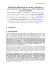
4.2. Schematic of Hydrodynamic Model
The EPD-RIV1H solves the hydrodynamic equations to provide time
histories of flows and water surface elevation. Since there is no analytical
solution to the governing equations, they must be solved numerically. The
solution scheme used in RIV1H is the widely known and accepted fourpoint implicit solution technique.
The method was first used by
Preissmann (1961) and is probably the most accepted and successful
procedure used today. It is also called a box scheme (Figure 4-1), where
n refers to time and j to space. The space derivatives and function values
are evaluated at an interior point of the box (n+θ)∆t, and terms of (n+1) ∆t
enter all of the equations. The result is a system of equations that must be
solved simultaneously. Since, as stated above, all of the non-linear terms
are retained, then the system of equations must be solved iteratively at
each step time. An initial estimate is made and then the equations solved
and results compared to the estimate. If they are acceptable (within some
criteria to test for convergence), then the solution proceeds to the next
time step, otherwise another iteration is made. Thus, the solution is
controlled in part by information provided by the user, including the:
time step,
converge criteria, and
weighting factor (θ)
The number of iterations allowed is presently set in the code to 200. If the
model does not converge on a solution within 200 iterations, it will stop
and write out diagnostic messages.
12
EPD-RIV1
VERSION 1.0
DRAFT: 4/10/02
∆ξ
D
n+1
t
t
Q
D
t
n
x
j
0
.
5
D
x
j+1
Figure 4-1 Four Point Implicit Solution Technique
The solution method (as determined by a Von Neumann stability analysis
by Fread, 1974, and Liggett and Cinge, 1975) is unconditionally stable
(theoretically) for 0.5 < θ < 1.0, and permits relatively unequal space and
time-steps. The scheme has second-order accuracy when θ = 0.5 and
first-order accuracy when θ = 1.0. It is unstable for 0.5 > θ. In practice
other factors may also contribute to the instability of the solution scheme.
The factors include dramatic changes in the channel cross-sectional
properties, abrupt changes in the channel slope and characteristics of the
flood wave itself. Thus, any model application should include an analysis
of the sensitivity of the accuracy of the solution to various time and
distance intervals (Barkau 1995).
The solution technique is implemented on a river system that has been
discretized by a network of time and space nodes separated by time and
space increments ∆t and ∆x. For example, the users must determine the
distance between nodes. Then, for each node they must apply
information about the cross-sectional shape, roughness, bottom elevation,
and initial conditions (the starting point for the first iteration) for flow and
depth.
The model is driven then by information specified at the boundaries of the
discretized grid (the boundary conditions). Some of the other factors
impacting the solution include:
13
EPD-RIV1
EPD-RIV1 USER’S GUIDE: DRAFT 4/10/02
Lateral and tributary inflow: runoff from lands adjacent to the
channel, point sources, or tributary inflow which can cause
increased levels of total mass and momentum in the river
Channel constrictions.
Often very intense channel
constrictions, due to bridges for example, occur over channel
lengths that are far too small to economically resolve in the
model. The effect of such constrictions is a momentum loss
and backwater effect, accounted for in the momentum equation
by subtracting a force term, based upon a user specified
coefficient, KE used in computing the head loss from
hE
KE  Q 
=
 
2g  A
2
Equation 4-3
The default value is zero for no constriction loss. A value for
KE as high as 0.5 may be appropriate for an abrupt
constriction.
Non-uniform velocities. When the velocity across the channel
is substantially non-uniform through the model reach (such as
in sharp bends), it may be necessary to use a momentum
correction factor β in the momentum equation. The
momentum correction factor β permits the use of the average
velocity in the solution whereas the velocity distribution at each
cross section may be quite different from the average. The
default value of 1.0 is recommended for rivers and streams.
Tributary networks. The momentum and continuity equations
above must be applied to each and every tributary entering the
main stem. At each junction, the water surfaces in each branch
must be equal. These are ”internal boundaries” and are
computed by the model.
Boundary conditions. The solution requires that boundary
conditions be specified for the upstream boundary (x = 0) and
the downstream boundary (x = L). The upstream boundary can
be either flows or depths. The downstream boundary may be
flows, depths, or a rating curve. It should be noted that the
14
EPD-RIV1
VERSION 1.0
DRAFT: 4/10/02
upstream boundary condition for a tributary can be selected by
specifying either the elevation or the flow. At the downstream
tributary boundary, i.e. the confluence with the main stem, only
the elevation is allowed as a "internal boundary" condition to
ensure that continuity is preserved at the junction. Internal
boundaries are computed by the model and not specified by the
user.
Given the above information, then the model will step through time, over a
period specified by the user, and compute a time history of downstream
flows and water surface elevations.
4.3. Data Preparation
One of the first tasks associated with a model application is the assembly
of the input data. This is a major task and may account for by far the
majority of the time and resources required for a model application. The
data required are those necessary to configure the model for a particular
system (geometric data), provide forcings to the model such as boundary
conditions and lateral inflows, and evaluate the model’s performance.
4.3.1. Geometric Data
4.3.1.1. MODEL GRID
One of the first tasks associated with preparing input for EPD-RIV1 is
assembling the geometric data. These data will be used to define the
characteristics of the waterbody and the computational grid used to
represent it. In RIV1, the waterbody is mapped onto a network consisting
of one or more branches. A branch is defined as a stretch of river whose
boundaries are a system boundary, a receiving stream, or a control
structure. For example, the branches may represent the main stem river
and its tributaries, or may represent lengths of the river which are
separated by a control structure such as a dam. Each branch is then
further subdivided into nodes, or locations in the river with known crosssectional characteristics which are separated from each other by a known
distance. The length between nodes, or cross-sections, may vary but that
variation should be gradual to minimize discretization errors. For example,
15
EPD-RIV1
EPD-RIV1 USER’S GUIDE: DRAFT 4/10/02
abrupt changes in cross-sectional area, roughness, lengths, etc. may
cause stability problems in both the hydrodynamic and quality model.
Factors affecting the computational grid. A number of factors must be
evaluated and weighed against each other when setting up the
computational grid. These include:
Boundary Conditions: The computational grid must be set
up so that the upstream boundary conditions, for both the
hydrodynamic (e.g. flows) and water quality model (e.g.
constituent inflow concentrations), are known and well
characterized. A common practice is to locate a boundary
where flow or water quality data are available, such as at USGS
gaging stations. It is also often best to locate model boundaries
at some point of control. A "control" is a location where there is
physical dependence between water surface elevation and
discharge, which may be a structure, constriction, or change in
bottom elevation. U.S. Geological Survey gage stations, for
example, are normally established at control points in a river.
Likewise, the downstream boundary must either be well
characterized or sufficiently below the area of interest so that
errors in its specification do not affect predictions in the area of
interest. Care needs to be exercised in establishing model
boundaries at areas which are not controls since unless flow is
uniform the discharge is not a function of elevation alone
(Henderson 1966).
Location of Control Structures: If there are control
structures within the system, such as dams with a controlled
release, then the grid must be broken into two or more
branches. Boundary conditions (such as a release) can only be
specified for a branch.
Tributary Impacts:
In many cases the impacts of
tributaries on the main river or stream can be described rather
than predicted. That is the user specifies the flows and
constituent concentrations for the tributary (e.g. in the lateral
inflow file read by EPD-RIV1). Alternatively, if the flows in the
main channel and tributary are linked in some way, or it is
necessary to predict (rather than describe) the flows and quality
of the tributary, then it may be necessary to include it in the
modeled grid as a separate branch.
16
EPD-RIV1
VERSION 1.0
DRAFT: 4/10/02
Travel time: A high degree of grid resolution is required in
some hydraulic studies, such as those used to evaluate
flooding potential. However, the resolution required to resolve
water quality gradients may be different. For example, a
material that decays at a rate of 0.1 day-1 will lose 10 percent of
its mass per day ( or require approximately 7 days to lose 50
percent of its mass and 23 days to lose 90 percent). Thus, if
the travel time through the entire grid is too short, it would be
necessary to increase the overall length (size) of the
computational grid in order to resolve the decay of the material,
and its possible impact on other materials. Conversely, if the
spacing between nodes within the grid is such that travel times
between them are short, it may be possible to reduce the
number of nodes without impacting water quality predictions.
Gradients: The spacing of nodes must be sufficient to allow
the model to capture gradients, in both hydraulic (e.g. depths
and velocities) and water quality characteristics. In general, if
the model is not capturing observed gradients, it may be
necessary to increase grid resolution.
Resource Requirements: The greater the number of
branches and nodes, the greater the memory and
computational time required to run the application and store
simulation results, and the more data required to support the
study. In general, it is often preferable to err on the side of
greater grid resolution. However, over specifying the grid may
result in unreasonable resource demands.
Data Defining the Computational Grid: Once the
extent of the grid has been determined, the identification and
connectivity of each branch included in the computation grid is
defined by specifying the following information:
Branch Name: provided for conveniently labeling the branch
Branch Number: used by the model for recognizing the
branch
17
EPD-RIV1
EPD-RIV1 USER’S GUIDE: DRAFT 4/10/02
Downstream Branch: either zero, if the branch terminates,
or the number of the branch it is connected to at its downstream
end
Downstream Node: specification of the down-stream crosssection allows the user to connect a branch to a location other
than the uppermost node of the downstream (receiving) branch.
For example, if the downstream branch for branch 1 was
branch 2, and the downstream node was 4, then the flows from
branch 1 would enter branch 2 at node 4 rather than node 1.
If there is no branch located above the particular branch, then the model
will expect an upstream boundary condition. If there is not a downstream
branch, then the model will expect a downstream boundary condition. If
two branches are connected, and the downstream node is zero, indicating
a control structure, then the user must specify a downstream boundary
condition. If the downstream node is non-zero, then the model will expect
a downstream head boundary condition and the model will compute the
boundary condition (an internal boundary) to insure that mass is
conserved.
Once the branches have been identified, then they are further subdivided
into nodes. There must be at least three nodes per branch. The
information required to define the individual nodes include their:
Name: provided for convenient recognition of the location of
the node,
Bed Elevation (ft): measured from some common datum,
Channel Length (ft): the distance along the river from this
node to the next node downstream.
4.3.1.2. CROSS-SECTIONAL DATA
Cross-sectional data are required to relate channel cross-sectional areas
and top-widths to depth and may be specified in RIV1H using common
shapes, as described by power equations, or by look-up tables of X,Y
pairs. The cross-sectional data provided as look-up data are provided in a
separate file from the main input to the model which contains the X and Y
coordinate data. RIV1H reads the cross-section coordinate data and uses
18
EPD-RIV1
VERSION 1.0
DRAFT: 4/10/02
them to generate a table of areas versus heights and widths. The model
also has the capability of developing the necessary cross-sectional data
for nodes where no information is available by "blending" information from
the upstream and downstream cross-sections. If data are only provided
for an upstream cross-section, the model assumes that the cross-section
of the downstream node is identical in shape.
RIV1H allows the cross-sectional shapes to be defined by a power
equation of the form of:
A = C1 H + C2 H C3
Equation 4-4
where A is the area (ft2), H stage (ft) and C1 to C3 are user supplied
coefficients.
This equation allows the user to describe a variety of
standard shapes, including rectangles, triangles and trapezoids. For
example, with C2 = 0 , they describe a rectangle of width C1. In cases
where an ellipse would give a better fit (for instance, flow in a partially full
conduit), C1 is half the vertical axis length, C2 is half the horizontal axis
length, and C3 is set to -1 to indicate to the program that an ellipsoid
description is intended. If C1 = C2 , of course, the cross section is circular.
One common problem in idealizing cross-sectional shapes is
discontinuities. Discontinuities may occur in very irregularly shaped cross
sections. Discontinuities are particularly common where it is necessary to
include the flood plain in computations. For such cases, it is preferable to
input surveyed cross-sectional data rather than using the idealized
equations described above.
19
EPD-RIV1
EPD-RIV1 USER’S GUIDE: DRAFT 4/10/02
X
Y
0
X
0
Y
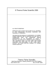
Figure 4-2
RIV1H can develop cross-sections’ shapes from survey data in two ways.
The simplest method develops a relationship for flow, area, and depth
from a set of X,Y pairs. A second method allows for development of the
necessary cross-section relationships by "blending" information from the
upstream and downstream cross sections (parent cross sections). In
cases where only one parent cross section exists, the computed cross
section is an exact copy of the parent. If there are no parent cross
sections, an error results.
RIV1H reads in the cross-section coordinate list and uses it to generate a
table of area versus height and width. The algorithm used allows cross
sections to be bumpy but they cannot fold in on themselves or have overhangs. The program inspects the data to make sure this is the case and
writes an error message if it is not.
Each tabulated cross section is given a name, which the model uses to
recognize the cross-sectional information, and a series of x and y
20
EPD-RIV1
VERSION 1.0
DRAFT: 4/10/02
coordinates (in feet) with the origin for x and y beginning at the top of the
left stream bank, where x increases to the right and y increases downward
when looking downstream (Figure 4-2). As with the algebraic method, the
channel bed elevation is understood to refer to the absolute lowest point in
the surveyed cross section.
4.3.2. Initial Conditions
Initial, or start up conditions, are required by RIV1H for both flow (ft3/sec)
and depth (ft ). The initial flow condition is usually some steady flow, such
as the base flow. The initial flow specified should also correspond to the
initial flows specified in the boundary condition, lateral inflow, and
withdrawal files. For example, if there is a large difference in flows
between the initial conditions and those in the first updates of the forcing
files, the model may become unstable. Similarly, the initial water surface
elevations should reflect the conditions expected for the initial flows.
Initial depths are often difficult to estimate from field data alone, except for
very simple systems, since they reflect the combined effect of the model
grid, bottom roughness and model forcings (inflows and withdrawals).
They may be obtained from previous hydraulic model applications, if
available. Otherwise, it may be necessary to make a best estimate of the
initial conditions, run the model under steady flow conditions, let the model
come to an equilibrium, and then use those results as the initial conditions
for subsequent simulations. If the initial estimates of depths are greatly
different from the equilibrium condition, the predicted values of the
hydraulic variables (flows, stages, etc) may oscillate. These results should
not be used in subsequent quality predictions. If greatly different, the
model may become unstable. The users must then examine the results
and determine the cause (e.g. location) of the instability and refine their
initial depth estimates until the model runs. See Section 4.4.5 Trouble
Shooting for additional information on start up errors.
4.3.3. Model Forcing Data
4.3.3.1.BOUNDARY CONDITIONS
There are two types of boundary conditions for RIV1H: External and
Internal. The Internal boundaries are computed by the model. For
example, in the case of an internal boundary formed by the junction of two
21
EPD-RIV1
EPD-RIV1 USER’S GUIDE: DRAFT 4/10/02
tributaries, RIV1H computes the water surface elevation and it is not
specified in input. External, or system, boundaries are at the ends of a
branch, such as the upstream and downstream ends of the main branch.
In order to solve the governing equations, a pair of boundary conditions,
one upstream and one downstream, must be known at all model time
steps.
Boundary condition information required by RIV1H includes, for the
upstream boundary
flows (ft3/sec), or
stage (ft),
and for the downstream boundary
flows (ft3/sec),
stage (ft), or
a rating curve.
For flow or stage boundary conditions the user may specify a constant
boundary value. If a constant value is not specified, then the model will
expect a time series of values to be read from an external file. In the
boundary condition the user specifies a date (day, month and year) and
time (decimal hours) for each value, and a separate file is prepared for
each boundary condition. The user specifies the branch that the file
contains the boundary condition for, whether it is an upstream or
downstream boundary, and the type of boundary that will be used. The
user also selects whether the model will linearly interpolate, or not,
between boundary updates.
Boundary data are required for both the upstream and downstream
boundary. As mentioned previously, in some cases it may not be critical
to specify the downstream boundary as accurately if it is located
sufficiently far downstream of the area of interest in the modeling study so
as not to influence it. This may be possible with rivers of moderate slopes,
but would almost never be the case where backwater effects occur within
the area of interest. For upstream boundaries, and for cases where the
downstream boundary is important, the boundaries drive the simulation
22
EPD-RIV1
VERSION 1.0
DRAFT: 4/10/02
and they must be as accurate and as complete as possible. If these data
are inaccurate, then the model predictions will be as well. It is a useless
exercise to attempt to calibrate the model to field data when the data used
to drive the model are inaccurate (Cole 1995).
Boundaries are usually located at some control point. They are also
usually located where data are available. For example, USGS gages are
usually located at control points (points where there is a unique
relationship between flows and water surface elevations) and used for
specifying boundary conditions.
The frequency at which the boundary conditions should be specified
depends upon gradients. That is, how frequently and by how much do the
flows change? For example, if the upstream boundary were a peaking
hydropower facility, then the flows may change rapidly (so must be
specified frequently) during generation and then be relatively constant
between generation periods (may be specified infrequently). Where much
of the inflow coming into the system through the upstream boundary is not
controlled, then frequent data may be required. For example, daily
averaged flows from gaging stations are usually not sufficient. Data
should usually be obtained on an hourly or more frequent basis. As with
the geometric data, it is usually best to err on the side of increased
frequency.
If a rating curve is specified as the downstream boundary condition, it
must be of the form:
H = COEFF
Q EXPO
where H is the depth of flow (ft), Q is the discharge (ft3/sec), and COEFF
and EXPO are specified by the user. These curves are often available
from state discharge data at gaging stations or from outfall relationships at
control structures such as dams and weirs. If the available rating curve is
of the form Q = aHb , then simply set EXPO = 1/b and COEF = a(-1/b) .
4.3.3.2.ROUGHNESS COEFFICIENTS
The bottom roughness is essentially a boundary condition to RIV1H and is
described using a roughness coefficient referred to here as Manning's n.
23
EPD-RIV1
EPD-RIV1 USER’S GUIDE: DRAFT 4/10/02
Manning’s n is the most commonly used means of describing bottom
roughness in hydraulic and hydrodynamic models and, although empirical,
is well known.
The user must estimate and provide RIV1H a value for Manning’s n at
each modeled node, or cross-section. A first approximation of Manning's n
for a particular application can be obtained from tabulated values, such as
those provided below. The user is also referred to Chow (1959), the
USACE (1959) and French (1985) for extensive tables of n values as a
function of channel type. The final values for a particular application are
often determined during the course of model calibration.
Table 4-1. Typical values for Manning’s n.
Type of Channel and Description
A. Natural Streams (top width at flood
stage < 100ft)
1. Streams on plain
a. Clean, straight, full stage, no rifts or deep pools
b. Same as above but more stones and weeds
c. Clean, winding, some pools and shoals
d. Same as above but some weeds and stones
e. Same as d but lower stages, more ineffective slopes and section
f. Same as d but more stones
g. Sluggish reaches, weedy, deep pools
h. Very weedy reaches, deep pools or floodways with heavy stands of
timber and underbrush
2. Mountain Streams, no vegetation in channel, banks usually steep, trees
and brush along banks submerged at high stages
a. Bottom with gravel, cobbles, and a few boulders
b. Bottom with cobbles and large boulders
B. Major Streams (top width at flood stage > 100 ft) (Note: the n value is
less than that for similar minor streams since banks offer less effective
resistance.
a. Regular section with no boulders or brush
b. Irregular and rough
Minimum
Normal Maximum
0.025
0.03
0.033
0.035
0.04
0.045
0.05
0.07
0.03
0.035
0.04
0.045
0.048
0.05
0.07
0.1
0.033
0.04
0.045
0.05
0.055
0.06
0.08
0.15
0.03
0.04
0.04
0.05
0.05
0.07
0.025
0.035
0.06
0.1
While it would be ideal to consider the Manning's n constant for a
particular river channel, in reality the roughness is highly variable. For
example, the value may vary with the depth of flow as different surfaces
come into contact with the water.
High values may be more
representative for shallow-depth conditions whereas lower values may be
appropriate for deeper flow. For example, shoal areas exhibit a variable n
that can have a significant effect on computed stage; at low stage, n is
usually larger than at high stage.
24
EPD-RIV1
VERSION 1.0
DRAFT: 4/10/02
For time-varying flow conditions, a variable Manning's coefficient may
have to be adjusted as a function of depth during the simulation. RIV1H
allows the user to vary n using the equation
n = a - b*H
Equation 4-5
where a and b are user supplied coefficients for each node and H is the
depth at that node. When the user initiates a simulation, the model first
sets n to the input value specified for the node. As the program executes,
n is adjusted with relation to depth over time. If at some point during the
execution, the value of n becomes less than 0.01, n is reset to 0.01 and a
message printed to the diagnostic file.
4.3.3.3.LATERAL INFLOWS
The lateral inflows specified to RIV1H include both point and non-point
sources. Data required to specify the lateral inflows are flows (ft3/sec), for
the hydrodynamic model, their associated concentrations, for the quality
model, and the location at which they enter the model network. There are
two alternatives provided for entering lateral inflow information: constant
and time-varying. The constant lateral inflows are specified along with
other node information (e.g. roughness coefficients, initial conditions, etc.).
The time-varying data are included as an auxiliary file. The flows from
both sources are added together by the model.
If time-varying lateral inflows are specified, the user must create an
auxiliary file containing a time series of flows (and concentrations for water
quality simulations). The flows and concentrations may be derived from
field or monitoring data or estimated by modeling. However, as with
boundary conditions, the data should be as frequent and accurate as
possible since they directly impact model predictions.
A relatively large number of point and non-point sources may commonly
enter the modeled system. The data available from the different sources
are often of varying frequencies and quality. However, to avoid the
management nightmare that would result from different files for each
source, and perhaps each constituent, only a single lateral inflow file may
be used in a simulation. The file specifies the nodes or cross-sections at
25
EPD-RIV1
EPD-RIV1 USER’S GUIDE: DRAFT 4/10/02
which the lateral inflows enter and then provides a time series of their
values (e.g. flows and concentrations, with only the flows being used in the
hydrodynamic predictions). Therefore, prior to inputting the data to
RIV1H, the lateral inflows must be processed so that all data are provided
at the same frequency. The evaluation of the data and processing of the
file is a major function of the DELIBERATOR, and the user is referred to
its description for guidance in accomplishing this task. The node at which
the inflow is specified to enter is the node number assigned by EPD-RIV1.
It is suggested that the model first be run and the node numbers obtained
from the output file.
The user may also enter scale and conversion factors for each node,
which have default values of one. The lateral inflow values multiplied by
the scale and conversion factors are used by the model. The user may
also elect to have the model linearly interpolate between update intervals
or not.
4.3.3.4.WITHDRAWALS
Withdrawals, where water is removed from the system, may also be
specified. The withdrawal flows are specified in an auxiliary file which
specifies the nodes where the withdrawals occur and a time series of the
flow values (ft3/sec). As with the lateral inflows, only a single withdrawal
file may be specified for a particular run. Therefore, all withdrawal flows
must be specified in this single file and all must be provided at the same
frequency. The DELIBERATOR may be used to synchronize multiple
withdrawal rates. The user may specify scale and conversion factors for
each withdrawal location, which have default values of one. The
withdrawal rates multiplied by the scale and conversion factors are used
by the model. The user may also elect to have the model linearly
interpolate between update intervals or not.
4.3.4. Hydraulic and Control Parameters
4.3.4.1.HYDRAULIC PARAMETERS
The hydraulic parameters specified in RIV1H include the gravitational
acceleration, two coefficients affecting the numerical solution, and a
momentum correction coefficient. The default value of acceleration
caused by gravity is set at 32.174 ft/sec2 under the assumption that the
units used in modeling are the customary English units. The water quality
26
EPD-RIV1
VERSION 1.0
DRAFT: 4/10/02
program does not accept input data with SI units, although it converts to SI
units.
The numerical method used by RIV1H is the four-point implicit method first
used by Preissman (1961) with subsequent applications by, among
others, Amein and Fang (1970) and Amein and Chu (1975). This
formulation is currently being used by Fread (1973, 1978) in the National
Weather Service Dambreak Model (Fread 1978). The method is weighted
implicitly at each time level, and the weighting coefficient (THETA) is
specified by the user. The method is unconditionally stable for 0.5 <
THETA < 1.0, and permits relatively unequal space and time-steps. The
scheme has second-order accuracy when THETA = 0.5 and first-order
accuracy when THETA = 1.0. A default value of 0.55 is cited in the
literature as optimal for model accuracy; however, a higher value (i.e., 0.6
to 0.75) is often used to enhance stability. It is recommended that the
user not use values outside of the range of 0.55 to 0.75.
The numerical method employed by the model uses an iterative approach
to obtain a solution to the non-linear equations. A tolerance factor
(TOLER) is specified by the user which the model uses to determine if the
answer has converged. The user will often notice that the model runs
faster when conditions are not changing, since the model requires fewer
iterations to converge. A maximum of 200 iterations is allowed before the
model stops execution and writes out an error message.
TOLER, is assigned a default value of 0.001. Iteration ceases when all
residuals (i.e., differences in successive iterations) for flow and area are
less than TOLER times the root mean square of all flows or areas in the
system. Experience suggests that often a larger value (i.e., 0.1) can be
used to reduce run time without substantially sacrificing accuracy.
When the velocity across the channel is substantially non-uniform through
the model reach, it may be necessary to use a momentum correction
factor (BETA) in the momentum equation. The momentum correction
factor permits the use of the average velocity whereas the velocity
distribution at each cross section may be quite different from the average.
It equals 1.0 for uniform flow (whereas 1.0 is no correction) and cannot be
less than 1.0. For RIV1H, a constant value is used throughout the
modeled reach. The default value of 1.0 is recommended for rivers and
streams.
27
EPD-RIV1
EPD-RIV1 USER’S GUIDE: DRAFT 4/10/02
4.3.4.2.CONTROL PARAMETERS
The control parameters include:
Start and End Times for the Simulation
Print Intervals, and
Time steps.
The start and end times specify whatever period the user want to simulate.
The user should make sure that there are data in the time series files (e.g.
boundary conditions, lateral inflows and withdrawals) for this period.
For the print intervals, the user specifies a date and then a frequency
(hours). The model will then print at that frequency until the next update.
This allows the users to vary the print interval over the simulation, if they
choose to do so. For example, they may want to print results more
frequently during the initial start up or during storm periods.
Similarly for the model time step, the user specifies a date an time step,
and that time step will be used between that date and the next specified.
One advantage of the implicit scheme used by RIV1H is that the time step
is not controlled by the Courant condition (see Section 4.4.5, Trouble
Shooting), which results in smaller time step limits under dynamic
conditions. A disadvantage of the numerical scheme is, however, that
there are not well defined limits to aid the user in determining what the
time step should be. Typical time steps are on the order of 15 to 30
minutes. In general, if the Froude number (a computed variable included
in the model output) is greater than one, the computed flows are
supercritical and the model should crash (become numerically unstable).
Also, while the hydrodynamic model is not limited by the Courant number,
the quality model is. So there may be situations where the hydrodynamic
model will run and produce accurate results which can not be used by the
quality model. Therefore, the user will want to adjust the time step (and/or
distance increments) so that the Courant number (also an output variable)
is less than one to avoid stability problems in the quality simulations. The
user should also adjust the time or spatial steps so that the Courant
number is reasonably close one to minimize phase errors. Longer time
steps may be possible for relatively steady flow conditions while smaller
time steps may be required under very dynamic conditions. See Section
4.4.5, Trouble Shooting, for additional information on the model time step.
28
EPD-RIV1
VERSION 1.0
DRAFT: 4/10/02
4.3.5. Calibration Data
The application of RIV1 also requires that data be available to calibrate
and the model and evaluate its predictions. While it is possible to apply
EPD-RIV1 without the use of calibration or evaluation data, it would not be
possible to estimate the uncertainty associated with that application. The
data usually consist of time series of hydraulic measurements, such as
flows
velocities, and/or
water surface elevations
at a series of points along the river which can be compared to model
predictions, graphically and statistically. Flow measurements provide a
means of checking your water balance to make sure that you are properly
accounting for all of the inflows and withdrawals. Velocities are a useful
check against model predictions. However, the user must remember that
the model is predicting a cross-sectionally averaged velocity. Water
surface elevations are most commonly used to check model predictions,
to insure that the model captures the timing, duration and peak of storm
waves, for example.
Another very good source of data are dye studies. Comparison with dye
concentrations can be accomplished after linking RIV1H with the quality
code (RIV1Q). The time-of-travel of the dye centroid provides a good
check of model hydraulic predictions. The dispersion of the dye cloud
provides a good check of the dispersion rates used in the quality model.
Generally, at least two sets of data are needed; often described as a set
for model calibration and a second, independent, data set for model
evaluation. However, this distinction is misleading since the modelers will
commonly use all of the data they have available to aid in defining the
system and testing the application. Ideally, the data should
contain one or more large events, and
29
EPD-RIV1
EPD-RIV1 USER’S GUIDE: DRAFT 4/10/02
contain periods of low flows,
It is usually best for the evaluation if sufficient data are available to test
model capabilities under conditions different from those used in the
calibration, or test the "robustness" of the application. For example,
geometric or cross-sectional data that may be adequate for one flow
condition may not be adequate for another; a condition that may only be
detected where sufficient data are available to evaluate the model under a
variety of flow conditions.
Where field studies are planned to obtain the calibration data, it is
important to remember that the model predictions are only as good as the
data used to drive the model. For example, it would be a useless exercise
to calibrate the model when the boundary forcings are not well known.
Ideally, the availability of adequate data should be assessed prior to
beginning the modeling study. If sufficient data are not available, then
plans should be made for obtaining them. In many cases, an iterative
approach is often useful. That is, the sampling plan can be designed with
the model in mind. Initial model simulations may aid in evaluating and
identifying deficiencies in the data, which can be corrected in subsequent
studies.
4.4. Simulations
4.4.1. Model Preparation
Once the data have been gathered, they are used to prepare input data
sets for the model. The function of the Deliberator and pre-processor are
to aid the user in the preparation of these files. The reader should refer to
the sections dealing specifically with those programs for a detailed
description of their use. The preparation begins with the creation of a
project file. The project file contains the names and locations of the main
input data sets and the auxiliary files. The files may exist or the user can
create them from scratch. The files that may be used to control simulation
include:
Main input control file (required): contains information on the
simulation period, print controls, time steps, beginning river
mile, hydraulic parameters, branch names, and specification of
the connectivity of branches and their boundary conditions.
Then for each branch, and for each cross-section (node) within
30
EPD-RIV1
VERSION 1.0
DRAFT: 4/10/02
a branch, an input screen is provided for a descriptive name of
the cross-section, the name of the cross-section used in the
look up tables (if used), the lengths (distance to the next crosssection), initial flows and depths, bottom elevations, constant
lateral inflows, coefficients for the cross sectional area (if used
instead of look up tables), depth variations in Manning’s n, the
momentum correction coefficient, and Manning’s n.
The remainder of the files are referred to as auxiliary files. They are not
required for a simulation, and are only included where needed. For
example, a constant flow may be specified for the upstream boundary in
the main control file. If a constant value is specified, then a boundary file
is not needed. Similarly, if the cross-section shapes (areas) are specified
using the area equations, a look up table is not required. Time-varying
lateral inflows and withdrawals are only specified where required. The
auxiliary files include:
Lateral Inflow File (One file only):
♦ locations (node numbers) receiving lateral inflow
♦ interpolation option (stair-stepped or linear)
♦ dates (year, month, day, decimal hour) and flows (cfs)
Withdrawal File (One file only):
♦ locations (node numbers) for the withdrawal
♦ interpolation option (stair-stepped or linear)
♦ dates (year, month, day, decimal hour) and withdrawal flows
(cfs)
Boundary Condition File (Separate files for each boundary
condition):
♦ branch to which boundary applies
♦ interpolation option (stair-stepped or linear)
31
EPD-RIV1
EPD-RIV1 USER’S GUIDE: DRAFT 4/10/02
♦ dates (year, month, day, decimal hour) and flows (cfs) or
depths (ft)
Cross-Sectional File
♦ names of cross-section
♦ y-x pairs of cross-sectional data
4.4.2. Model Simulations
Once the input files are prepared, and the project file completed, the users
should return to the SHELL and select the project (Figure 4-3). The users
Figure 4-3
can then execute the model from either the file menu or by clicking on the
run icon for H (RIV1H). Before the model executes, the users will have to
respond to three questions:
1)
Do you want to create a report ?
2)
Do you want to write a hydrodynamic linkage file?
32
EPD-RIV1
VERSION 1.0
DRAFT: 4/10/02
3)
Do you want to write out time-varying data?
If the users say yes to the first question, they can fill out a form which
documents the simulation (Figure 4-4). Additional information describing
the input files, control information, and length of simulation will be
Figure 4-4
appended to the information the users provide. The users can then save
the file at the end of the simulation.
If the users say no to the second question, no hydrodynamic linkage file
will be created. Since this file may become large and writing to it takes
time, not electing to create it will save both disk space and simulation time.
For example, the users may not want to write this file during their initial
hydrodynamic simulations. It is of course required to have this file if they
then want to run the quality model.
If the users say yes to the third question, then information will be written to
the output file each time that time-varying information is updated from the
auxiliary files. This is usually only needed to aid in diagnosing errors.
33
EPD-RIV1
EPD-RIV1 USER’S GUIDE: DRAFT 4/10/02
After these questions have been addressed, the model will execute.
During execution, intermediate model results will be displayed (Figure 45). The user may scroll through the model nodes or through the display
variables. If the users encounter a problem that they need to correct, that
may stop the program. Also, the priority of the job may be changed during
the simulation. The users may pause (stop) the simulation if they need to
do something else or may maximize the priority by putting the model in
turbo mode. The fastest run times will occur if they shut off the writing of
the intermediate simulation results and turn the model to turbo.
Once the simulation is complete, the grid will disappear and they will be
back in the shell. If the users created a report, they will be asked to save it
at this time. The users may then view the output files or graph the
simulation results.
4.4.3. Model Output
The output from the model includes the intermediate screen results and
the simulation report. Additional files created that the users can view
include:
Output File: This file mimics the input. When created, it will
have the same name as the master input file but with the
extension *.OUT. It contains much of the same information as
the report prepared by the pre-processor. In addition, there are
diagnostic messages which are written to this file. It is a text file
that must be examined by an editor or word-processor (for
convenience the users should put their favorite editor on the
tool menu in the SHELL).
34
EPD-RIV1
VERSION 1.0
DRAFT: 4/10/02
Figure 4-5
Graphics File: A graphics file will be created with the same
name as the master input file but with the extension *.BMD. The
graphics file is used by the post-processor and contains the
same result information as is written to the screen during
runtime. The output includes both variables that are computed
as part of the model solution (e.g. flows and water surface
elevations) and those intended to aid the user in evaluation of
the model results (e.g. Froude and Courant numbers). The
following information is written to the file at the frequency
specified by the user for each selected model node:
Flow (cfs)
Surface Elevation (ft)
Velocity (ft/sec)
35
EPD-RIV1
EPD-RIV1 USER’S GUIDE: DRAFT 4/10/02
Froude Number
Courant Number
Lateral Withdrawal (cfs)
Mannings n
Width (ft)
Area (ft)
Constant Lateral Inflow (cfs)
Time Varying Lateral Inflow (cfs)
Hydraulic Depth (Area/Depth, ft)
Depth (ft)
Time Step (sec)
Error File: This file will have the same name as the master
input file but with the extension *.ERR. It contains diagnostic
information. For example, it will write out information to identify
problem locations as the number of iterations approaches the
maximum.
Linkage File: This file will also have the same name as the
master input file but with the extension *.HYD. This is the
hydrodynamic linkage file. It contains all of the morphometric
and transport information needed by the quality model.
4.4.4. Model Calibration
Calibration usually refers to the identification of site-specific values for
coefficients as obtained by varying model coefficients until good
agreement is obtained between observed and predicted data. The
36
EPD-RIV1
VERSION 1.0
DRAFT: 4/10/02
objective of the calibration is to reproduce observed data at an acceptable
level of accuracy.
The first step of the calibration process is usually just to test the model
setup to insure that the model will run and produce meaningful results.
Since the users have complete control over their model system, they
should try to produce simulations with known results. The simulations
could be under steady flow conditions, for example. If errors are identified,
then modification of the grid, time step, or hydraulic control parameters
may be required (see Section 4.4.5: Trouble Shooting).
In the calibration process, comparisons are usually made between
observed and predicted stage, rather than flow. Flow is a derived quantity
(for example from stage/discharge relationships). However, comparisons
of flow are still useful for making sure that all of the water is accounted for
(completing a check of the water balance). Comparisons of velocities
(unless they represent averaged values) are of lesser usefulness.
Comparison to dye concentrations (by linking the hydrodynamic results to
the quality model) is also a very good check on model predictions.
Some of the problems often encountered in calibration are that the model
will not reproduce either the timing or shape of a downstream hydrograph
or it will work well for one set of conditions and not another. In RIV1H the
only coefficients that are typically varied during the course of the
calibration are the bottom roughness coefficients (Manning’s n).
Manning’s n may be adjusted within a relatively narrow range, as defined
by the literature values for a certain stream type (see Section 4.3.3.2).
The impacts of increasing Manning’s n are to
increase travel times, and
reduce flood flows and elevations.
The user may adjust Manning’s n to match both high and low flow periods
of an event. In some cases it may be necessary to increase Manning’s n
during high flows using the stage relationship to compensate for the
increased roughness of overbank areas.
37
EPD-RIV1
EPD-RIV1 USER’S GUIDE: DRAFT 4/10/02
The remainder of the calibration exercise is really a testing exercise for the
geometry and boundary forcings. If good agreement can not be obtained
through adjustment of Manning’s n, then the user must become a
detective to determine what is causing the problem. It is usually because
something was incorrectly specified or left out. For example, errors in the
geometric characterization or estimates of bottom slopes may prevent the
model from accurately predicting variations in water surface elevations.
These errors may only become apparent when the model predictions are
compared to field data. The errors may also lie in the calibration data or
result from some unique event that occurred during the period the
calibration data were collected.
The users should not assume that the hydrodynamic calibration is
complete until they have conducted tests with the quality model. For
example, errors that are not apparent in comparisons with water surface
elevations may become apparent when examining water quality
concentrations. Errors or problems with the quality simulation may require
the user to return to, and refine, the hydrodynamic model application.
4.4.5. Trouble Shooting
RIV1H is a very robust model capable of simulating a wide variety of
dynamic conditions in streams and rivers. However, when running the
model the user may encounter start up or stability problems that have to
be corrected before meaningful results can be achieved. These problems
may be evidenced by the model failing to converge on a solution,
producing negative depths or “going dry”. That is, the model will not run at
all or will “crash” under certain conditions. Problems can also result in
numerical oscillations in model predictions. In these situations, the model
will run but will produce answers that are not meaningful. The oscillations
can be detected by carefully examining the output of RIV1H. In some
cases the problems can also be detected when running conservative
tracer tests with the quality code (RIV1Q). Problems during model start up
can result from incorrect morphometry or poor initial conditions. Phase
errors can also occur associated with unsteady flow waves. Streams with
riffle sections accentuate these problems.
All one-dimensional hydrodynamic models have difficulty simulating
systems with steep slopes, such as mountain streams. If the flow
becomes supercritical, then the model may crash or not be able to
converge on a solution. One measure of critical flows is the Froude
number (Fr),
38
EPD-RIV1
VERSION 1.0
DRAFT: 4/10/02
Fr
=
 Q
 
 A
g
A
B
Equation 4-6
where Q is the flow, A the cross-sectional area, B the top width and g
gravitational acceleration. If Fr > 1, then the flow is supercritical. This
condition will result in instabilities in RIV1Q even if RIV1H runs. The user
may elect to either “smooth” the slope to remove these conditions or
increase the bottom roughness coefficient to increase drag in the area
where supercritical flows are encountered.
If inaccurate initial depths are selected for the initial flows, the model will
have trouble getting started. This may be evidenced by the model
becoming unstable as evidenced by it failing to converge, computing
negative depths or “going dry.” If the users encounter these errors when
they first start the model they must first have to determine where and why
the problem occurs. They may want to reduce the print interval at the
beginning of the simulation to write out results very frequently so they can
be examined to determine the cause of the start up problem. Poor
estimates of initial conditions can be particularly problematic where it is
necessary to specify flows at the downstream boundary (for example for
specifying the controlled outflows from a structure). This situation should
be avoided if possible.
Estimates of initial depths may be available from previous modeling or
field studies, or steady flow hydraulic models. If good initial estimates of
depths are not available, it is best to run the model for a steady-state flow
condition using deeper than expected conditions. If lateral inflows and
outflows are significant, it may be necessary to include them in these
simulations as well. If head is specified downstream, then the head may
be likewise initially greater than the expected condition and then
correspondingly gradually decreased toward the expected condition.
With a constant inflow rate and using a rating curve downstream, or head,
the water surface in the segment will eventually drop to a steady-state
water surface profile corresponding to that flow, channel geometry, and
bed roughness. If problems are still encountered starting the model, the
use of small time-steps, at least initially, has helped. After a steady-state
39
EPD-RIV1
EPD-RIV1 USER’S GUIDE: DRAFT 4/10/02
flow and water surface profile have been achieved, it is best to use these
results to start subsequent simulations.
Problems may also be encountered when using tabulated cross-sections
where either there are multiple x-coordinates with the same y coordinate,
which may result in a division by zero in the computation of areas, or
where there are large changes in widths over short vertical distances. For
example, if the predicted water surface elevation is just at the point where
a large change in width (and subsequently area) occurs, then the solution
may oscillate just above and just below that point and fail to converge. For
such a case it may be necessary to smooth this transition. If a division by
zero error is encountered in the area computation, the user may need to
increment the y-value slightly. The model error output provides the
location of an instability to aid the user in identifying where the problem
occurred. However, the problem may not actually be at the locations
where the instability occurred, but may, for example, be just upstream.
Phase errors, which may accompany unsteady flow waves, can result in
negative depths (usually in or near shallow riffle sections). If this happens,
a fatal execution error occurs, and the program is stopped. Several things
can be done to eliminate this problem. First, make sure that the
cross-sectional area is adequately described, especially at low stage.
Next, check the value of THETA (see Section 4.3.4.1: Hydraulic
Parameters); a higher value (e.g. 0.75) may help. If problems are still
encountered, it may be necessary to change the time-step such that the
surface wave Courant number is closer to 1.0. As values of this number
decrease below or increase above 1.0, phase errors become worse (Lyn
and Goodwin 1987, Liggett and Cunge 1975). The surface Courant
number is defined as
Cr
=
∆x
Us ∆ t
Equation 4-7
where Us is the speed of the surface wave (=
gH where H is the depth
and g gravitational acceleration), ∆t is the time-step size and ∆x is the
spatial step size. The Courant number also limits the time step that can
be used in the quality model. So, the user should also adjust the time step
so that a number less than one is achieved throughout the simulation prior
to linking the hydrodynamic and quality model. The same result can be
40
EPD-RIV1
VERSION 1.0
DRAFT: 4/10/02
achieved by adjustment of the spatial steps. The Courant number is
computed by the model and provided in model output.
Large variations in spatial steps, bottom slopes, roughness coefficients
(Manning’s n), or cross-sectional characteristics between nodes may also
cause the hydrodynamic and/or the quality model to become unstable or
produce phase errors (such as overshooting or undershooting the correct
values). Abrupt changes in the flood wave itself can also cause problems.
If adjusting the time or spatial step does not solve the problem, the user
should smooth these transitions. Ramping of the inflow hydrograph to
yield a gentler, longer wave will usually reduce phase errors since the
unsteady flow waves are more spread out. As an example, hydropower
turbines can come up to full power in about 5 min; peaking hydropower
releases can result in highly unsteady flow waves in the receiving stream.
It may be necessary to spread out the generation start-up over 15 to
30 min.
Judicious smoothing of the inflow hydrograph can be
accomplished without jeopardizing study objectives. Judicious smoothing
of the changes in the characteristics (slope, roughness, areas, etc.)
between cross-sections may also be required.
4.4.6. Linkage with Water Quality
The linkage of the hydrodynamic model with the quality model is relatively
transparent to the users. They need only to indicate at runtime that a
hydrodynamic linkage file should be created. The hydrodynamic linkage
file contains all the information the quality model needs to define the
model grid. For each hydrodynamic time step, the file contains the time
step, and then for each cross-section or node, the flows, time-varying
lateral inflows, water surface elevations, areas, and widths. The period of
the quality simulation needs to lie within the period for the hydrodynamic
simulation, but they need not be identical. The model will begin the
simulation at the latest of the two specified start times (one for the
hydrodynamic and one for the water quality model) and end at the earliest
of the two specified end times. The quality simulations can then be made
within any window of the period of the hydrodynamic simulation.
The quality model will generally assume that the hydrodynamic linkage file
it will use will have the name of the hydrodynamic input file specified in the
project file, but with the extension *.HYD. However, the user will be
41
EPD-RIV1
EPD-RIV1 USER’S GUIDE: DRAFT 4/10/02
prompted at runtime to determine if they want to use some other linkage
file.
5.
Model Application: Water Quality
5.1. Overview of Solution of Mass Balance Equations
The quality component of CE-QUAL-RIV1 (RIV1Q) was designed to
simulate quality variations in river systems under highly unsteady flow
conditions. Since the speed of flow waves is often quite high, water quality
concentrations can be dominated by advective transport but affected by
biogeochemical interactions and diffusion. Therefore, the water quality
model is dynamic and has the following attributes. The model:
Accounts for time-varying flow, elevation, and water quality
constituent changes resulting from highly unsteady flows.
Includes the direct explicit interaction of flow and elevation on
the constituent distributions.
Is applicable to a river channel of arbitrary cross section and
specified bottom slope.
Allows for a number of water quality constituents and the proper
mathematical
specification
of
their
mathematical
interrelationship.
Accounts for the effects of lateral inputs of water and
associated pollutant concentrations.
Allows simulations of multiple hydraulic control structures.
The basic equation solved by RIV1H is the based upon the conservation
of mass: a statement that the rate of change of mass stored in a system
must equal the quantities of mass entering a system (i.e. due to transport,
loads or internal reactions) minus the mass leaving the system due to
transport, transformation or degradation. For a one-dimensional system,
after some manipulation, the conservation equation may be written as:
42
EPD-RIV1
VERSION 1.0
DRAFT: 4/10/02
∂α
∂α
∂2 α q
+ u
= D
+ (γ - α ) - Ks α + SINKS
∂t
∂x
∂ x2 A
Equation 5-1
where:
α
u
x
q
D
γ
Ks
SINKS
=
=
=
=
=
=
=
=
constituent (i.e. dissolved oxygen, temperature, etc.)
velocity
longitudinal distance
lateral inflow rate
dispersion coefficient
concentration of the runoff input to the channel by distributed flow q
biochemical uptake or decay rates (+) and growth rates (-)
biochemical sources (+) and sinks (-)
The first term on the left hand side of the above equation represents the
time rate of change of constituent concentration. The second term
represents advection of the constituent. On the right hand side, the terms
represent diffusion, lateral loadings (or withdrawals), reactions and
sources/sinks. The reactions are those effecting the particular constituent,
such as decay or decomposition. The source and sink terms may
represent sources from other constituents (e.g. nitrification is a reaction
term for ammonia and a source term for nitrate) or external sources (e.g.
surface heat exchange is a source term for temperature). When solved,
the mass balance equation permits the calculation of downstream
histories of constituent concentrations.
5.2. Schematic of Water Quality Model
The water quality component of CE-QUAL-RIV1 (RIV1Q) was designed to
combine hydraulic information received from RIV1H with mathematical
specifications of the kinetics of, and interrelationships between, water
quality constituents in order to simulate variations in water quality under
highly unsteady flow conditions.
5.2.1. Solution Scheme
As with the hydrodynamic model, since there is no analytical solution to
the governing equations except for very simplistic conditions, they must be
solved numerically. Since any number of species could conceivably be
43
EPD-RIV1
EPD-RIV1 USER’S GUIDE: DRAFT 4/10/02
solved for, the numerical solution must be as quick as possible. This suggests the use of explicit time-marching procedures. However, simple
explicit (and also simple implicit methods) time marching for the advection
problem is a very severe test for which, unfortunately, the simple methods
fail to provide the desired accuracy. Pure advection is the single most
difficult test for a numerical method since the initial concentration
distribution imposed on the problem must be numerically advected or
transported without loss of mass, shape, and peak value, or distortion of
the statistics of the distribution including mean, variance, skew, and
kurtosis.
A powerful and accurate explicit method based upon a compact, but
fourth-order accurate, numerical expression is used to solve Equation 5-1
for advection. The compact, fourth-order accurate scheme presented by
Holly and Preissman (1978) is used for all advective mass transport
calculations. An implicit fractional step method is subsequently used for
the dispersion term.
5.2.2. Water Quality Kinetics
Equation 5-1 applies to all water quality constituents. What defines a
particular constituent are the concentrations assigned to the boundaries
and lateral inflows and the number and kind of reactions and
sources/sinks. The transport variables (velocities, flows, areas, etc.) are
common to all water quality constituents.
44
EPD-RIV1
VERSION 1.0
DRAFT: 4/10/02
Atmosphere
DO demand
only if
NBOD not
simulated
Temperature
nitrification
Nitrate-N
release
denitrification
NBOD
settling
Macrophytes
death
oxidation
respiration
Manganese
Organic-N
death
photosynthesis
settling
Iron
hydrolysis
Algae
death
CBOD
(Types 1 & 2)
settling
benthic
release
uptake
uptake
sediment
denitrification
nitrate
reduction
Ammonia-N
Organic-P
Inorganic-P
Dissolved
Oxygen
sediment
demand
uptake
settling
benthic
release
reaeration
Atmosphere
Coliform
Bacteria
death
Arbitrary
Constituents
(Types 1 and 2)
death or
decay
Figure 5-1
RIV1Q has the capability of simulating variations in up to the 16 state
variables, and the interrelationships between these are illustrated in Figure
5-1. RIV1Q can also exclude any of these state variables from
simulations.
The rate of variation for each state variable, and the interactions between
them, are determined using specified kinetic rate and stoichiometric
coefficients. The kinetic rate coefficients are input by the user. Some of
the coefficients and kinetic rates are assumed to be constant over the
system (global values), while others may be varied between branches or
between individual cross sections.
A brief discussion of the kinetic transformations for each state variable is
provided below. detailed discussion of the interrelationships is provided in
Section 7.3.
45
EPD-RIV1
EPD-RIV1 USER’S GUIDE: DRAFT 4/10/02
5.2.2.1.TEMPERATURE AND SOLAR RADIATION
Temperature simulations are based on either a full heat balance or a
simple equilibrium temperature approach. Using the full heat balance
approach, each term in the heat balance equation is computed, based on
algorithms from the QUAL2 model (Brown and Barnwell 1987), including:
net short-wave radiation, net long-wave radiation, heat loss due to
evaporation, and heat transferred by conduction at the water surface and
bottom. The net effect of these individual components of the heat balance
is then used by RIV1Q to compute a change in temperature. The
computations in the full heat balance depend upon: water temperature;
time of the year and day; site latitude, longitude, and elevation; and local
meteorological data. The water temperature used in the computations is
that predicted during the previous model time step. The time-varying
meteorological data are read from external files by RIV1Q. Different
meteorological conditions can be assigned to different portions of the
model grid, with a limit of five sets of meteorological data. The effect of
canopy or bank shading may be simulated by specifying a shading
coefficient, and the computed solar radiation is reduced by one minus that
fraction.
In the equilibrium temperature approach, the net effects of the individual
terms in the heat balance are computed externally to the model and
incorporated into an equilibrium temperature and coefficient of heat
exchange. The equilibrium temperature is that temperature which will be
achieved when the water reaches an equilibrium with the meteorological
conditions and the coefficient of heat exchange reflects the rate at which
that equilibrium will be achieved. Presently in RIV1Q, the equilibrium
temperature and coefficient of heat exchange are constants. That is they
are not allowed to vary with time.
Time-varying solar radiation is computed by RIV1Q when the full heat
balance option is selected, based upon the time of the day and year; local
latitude and longitude; cloud cover, and a specified dust attenuation
coefficient. Under the equilibrium temperature approach, solar radiation is
not predicted. Dawn, sunset and the daily noon light intensity are
specified as constants and then the light during daylight hours estimated
using a sine curve. The attenuation of solar radiation through the water
column is computed using an extinction coefficient reflecting a base value
to which is added the effect of algal self-shading, using an expression
extracted from the QUAL2 model.
46
EPD-RIV1
VERSION 1.0
DRAFT: 4/10/02
5.2.2.2.DISSOLVED OXYGEN DYNAMICS
Dissolved oxygen is transferred by reaeration, produced by algae and
macrophytes, consumed by the death of algae and macrophytes;
consumed by nitrification or nitrogenous biochemical oxygen demand;
consumed by sediment oxygen demands; and consumed by CBOD
(Types 1 and 2), iron, and manganese oxidation (Figure 5-1). A certain
fraction (user specified) of the algal and macrophyte mortality is assumed
to contribute to CBOD. The remainder is assumed to be oxidized
immediately, producing an oxygen demand. The consumption and
production of oxygen by algal and macrophyte productivity and death, as
well as by nitrification and oxidation, are related to other state variables
through stoichiometric coefficients.
The stoichiometric coefficients
affecting dissolved oxygen utilization are specified by the user.
Reaeration refers to the transfer of oxygen across the air-water interface.
This transfer is affected by the difference in dissolved oxygen
concentrations between the air and water as well as by the turbulence in
the film of water adjacent to the surface. The turbulence in that thin film
may be due to wind shear or shear produced by the water currents and
controls the rate of transfer. The rate of wind driven reaeration is
computed in a subroutine based on O'Conner's (1983) formulations. The
rate of reaeration due to current shear is computed in RIV1Q using either:
Tsivoglou-Wallace formulation.
An empirical expression in which the user specifies the
coefficients. The default values of the coefficients are those for
O'Connor-Dobbins.
Covar’s method.
A user specified coefficient, which may be varied by node.
Oxygen solubility is computed from Elmore and Hayes (1960) or using
APHA's 1985 DO saturation equation, as a user option. At the option of
the user, the DO saturation may also be corrected for elevation.
47
EPD-RIV1
EPD-RIV1 USER’S GUIDE: DRAFT 4/10/02
Reaeration may also occur as water passes over or through control
structures. Structural reaeration may be simulated using Wilhelm's
equation (Wilhelm, S.C. and Smith, D.R. 1981. Reaeration Through
Gated-Conduit Outlet Works. Technical Rept. E-81-5. US Army Engineer
Waterways Experiment Station, Vicksburg, Mississippi).
Sediment oxygen demand (SOD) is not simulated by RIV1Q. Rather, the
effects of SOD on dissolved oxygen are computed from user specified
rates, which can be varied between nodes or cross sections. The rates
are then adjusted according to the local depth and temperature. The
effect of temperature is computed using a temperature coefficient input by
the user.
5.2.2.3.BIOCHEMICAL OXYGEN DEMAND
There are three forms of BOD that may be simulated with EPD-RIV1, two
forms of carbonaceous BOD and NBOD (Figure 5-1). All of the forms
simulated are the ultimate BODs. The CBOD represents the amount (as
chemically equivalent oxygen) of biodegradable organic matter present,
excluding organic nitrogen. The CBOD (ultimate) is simulated using kinetic
losses due to aerobic oxidation (temperature corrected), anaerobic
oxidation by nitrate reduction (denitrification), and settling. A user
specified fraction of the decaying algae and macrophytes are assumed to
contribute to CBOD (using a specified fraction), the remainder being
oxidized immediately.
The kinetic loss of CBOD due to oxidation is estimated from a user
specified rate which is then adjusted according to dissolved oxygen
concentrations. The rate of CBOD decay may approach zero as dissolved
oxygen approaches zero, as computed using a user specified dissolved
oxygen concentration at which CBOD decay is at one-half its maximum
rate. Conversely, the rate of denitrification may increase toward its
maximum rate as dissolved oxygen and nitrate concentrations approach
zero. Therefore, in the absence of oxygen and nitrate there is no CBOD
removal. The rates of oxidation CBOD and denitrification are also
adjusted according to the effects of temperature using a Q10 formulation.
Nitrogenous biochemical oxygen demand (NBOD) is treated similarly to
CBOD. The NBOD (ultimate) is simulated using kinetic losses due to
aerobic oxidation (temperature corrected) and settling. The kinetic loss of
NBOD due to oxidation is estimated from a user specified rate which is
then adjusted according to dissolved oxygen concentrations and
temperature. The rate of NBOD decay may approach zero as dissolved
48
EPD-RIV1
VERSION 1.0
DRAFT: 4/10/02
oxygen approaches zero, as computed using a user specified dissolved
oxygen concentration at which NBOD decay is at one-half its maximum
rate. To avoid “double-dipping”, if NBOD is simulated (not by-passed),
then dissolved oxygen concentrations are reduced by NBOD but not by
nitrification of ammonia.
5.2.2.4.ALGAE
Algae are modeled as a state variable (subject to transport) in RIV1Q
(Figure 5-1). The rate of algal growth is computed from a specified
maximum growth rate which is modified by available light. Algal growth is
also limited by nitrogen (ammonia and nitrate) and inorganic phosphorus.
RIV1Q uses a multiplicative approach for light and nutrient limitations to
growth, similar to that in QUAL2 (instead of a minimum). Algal death
occurs continuously and is modified according to dissolved oxygen
concentrations. The user may specify a dissolved oxygen concentration
at which death occurs at one-half of its maximum rate, which is then used
to correct the rate of algal death.
5.2.2.5.MACROPHYTES
While the effects of macrophytes are included in RIV1Q, macrophytes are
not modeled as a state variable (subject to transport, Figure 5-1).
macrophytes were added primarily to include their impacts on dissolved
oxygen and nutrient cycling in rivers.
The effects of macrophyte growth on the RIV1Q state variables are
computed from the product of a specified macrophyte density and a
specified growth rate. The growth rate is modified by the availability of
light, which may vary over the course of the day, allowing simulation of diel
variations. Unlike algae, the rate of macrophyte growth is not limited by
nutrient availability in RIV1Q, since macrophytes can theoretically obtain
nutrients from the sediments (which is not modeled) as well as the water
column. The rate of macrophyte death is estimated from the product of
the a specified macrophyte density and death rate. An option is included
to reduce the rate of death, or decay, as dissolved oxygen concentrations
approach zero, through a user specified dissolved oxygen half-saturation
constant.
49
EPD-RIV1
EPD-RIV1 USER’S GUIDE: DRAFT 4/10/02
5.2.2.6.PHOSPHORUS SPECIES
RIV1Q simulates organic phosphorus and phosphate, or inorganic
phosphorus (Figure 5-1). Organic phosphorus is produced by the decay
of algae and macrophytes and lost due to decay and settling. The
production of organic phosphorus by algal and macrophyte death is
computed using a stoichiometric coefficient representing an assumed
phosphorus content.
Phosphate is lost due to uptake during algal and macrophyte growth and
gained due to sediment release and the decay of organic phosphorus.
Sediment releases of phosphorus are computed from user specified rates.
The rates are then adjusted according to the local depth and temperature.
The effect of temperature is computed using a Q10 formulation, where the
temperature coefficient is input by the user.
5.2.2.7.NITROGEN SPECIES
RIV1Q simulates organic nitrogen, ammonia and nitrate-nitrogen (Figure
5-1).
Organic nitrogen is produced by the decay of algae and
macrophytes and lost due to hydrolysis, nitrate reduction (denitrification)
and settling. The production of organic nitrogen by algal and macrophyte
death is computed using a stoichiometric coefficient representing an
assumed nitrogen content.
Ammonia-nitrogen is lost due to nitrification and uptake by algae and
macrophytes. The loss rate due to uptake is based on the fraction of
ammonia available as compared to nitrate-nitrogen. The rate of nitrification
is dependent upon temperature and dissolved oxygen concentrations.
The hydrolysis of organic nitrogen represents a source term for ammonia,
as does the death of algae and macrophytes. Sediment releases of
ammonia-nitrogen are computed from user specified rates. The rates are
then adjusted according to the local depth and temperature. The effect of
temperature is computed using a Q10 formulation, where the temperature
coefficient is input by the user.
Nitrate-nitrogen is formed by nitrification of ammonia and removed by
denitrification in the sediments, denitrification (or anaerobic utilization of
CBOD) in the water column, and uptake by algae and macrophytes.
50
EPD-RIV1
VERSION 1.0
DRAFT: 4/10/02
5.2.2.8.IRON AND MANGANESE
As modeled by RIV1Q, iron and manganese have no autochthonous
sources. That is, they can enter the system only through boundary
conditions (upstream, tributary or lateral inflows). Their oxidation is treated
as a simple first-order loss, which is assumed not to occur if dissolved
oxygen concentrations fall below a user specified threshold value. The
first order rate constants are not temperature corrected. The effect of iron
and manganese oxidation on dissolved oxygen is included in the model.
5.2.2.9.COLIFORM BACTERIA
As with iron and manganese, coliform bacteria are assumed by RIV1Q to
have no autochthonous sources. That is, they can enter the system only
through boundary conditions (upstream, tributary or lateral inflows). Their
mortality is treated as a simple first-order loss, which is temperature
corrected using a Q10 formulation.
5.2.2.10.ARBITRARY SUBSTANCES
There are two arbitrary constituents included in the model. They may be
either conservative or decay according to first order rates specified by the
user, which may be temperature corrected. As with coliforms, the arbitrary
constituents are assumed to have no autochthonous sources.
5.3. Data Preparation
5.3.1. Linkage with Hydrodynamic Model
A hydrodynamic linkage file is required in order to run RIV1Q. The user
must have created a hydrodynamic input file, run the hydrodynamic
model, and created a linkage file prior to running the quality program. The
quality code gets all of the transport information from this file. The quality
file must have the same number of branches and nodes as the
hydrodynamic file. At runtime, the default linkage file will be one with the
same name as the hydrodynamic input file specified in the project, with the
extension *.HYD. However, the users will be prompted to allow them to
select an alternative linkage file.
51
EPD-RIV1
EPD-RIV1 USER’S GUIDE: DRAFT 4/10/02
5.3.2. Kinetic Data
Each of the arrows in Figure 5-1 represents a kinetic process that
proceeds at a rate which is controlled by the user through their input of
kinetic data. The kinetic data include rate constants, which indicate the
rate at which the kinetic process proceeds (e.g. nitrification rates, CBOD
decay rates, etc.). There are also coefficients for correcting rates due to
variations in temperature and dissolved oxygen concentrations. The
kinetic data include stoichiometric constants, relating the content of one
variable to another, such as the nutrient content of algae. The kinetic data
also include options whereby the user may select a particular method for
computing a kinetic rate, such as the rate of reaeration.
Some of the rates are global, meaning that they can not be varied over the
model domain. Others may be varied by branch and a few can be varied
between individual nodes.
There are a relatively large number of kinetic data that may be specified
by the user. It is doubtful that all of the available coefficients would be
needed for any specific application. The number and type of kinetic data
required depend upon the state variables being simulated and the needs
of the specific application. The kinetic data that may be specified for each
state variable and kinetic process are discussed in detail in Section 7.3.
5.3.3. Initial Conditions
The user must provide initial concentrations for each of the state variables
they are simulating at every node in the system. Accurate initial conditions
are only meaningful until they are flushed out of the system. Therefore, as
the flushing time becomes short, the relative importance of having
accurate initial conditions becomes less. For systems with short flushing
times with respect to the length of the simulation, the user may often either
ignore the model predictions until after the first few flushing times or run
the model using their initial boundaries and loadings and use those
predictions for their initial conditions. For a system with a long retention
time, having accurate initial conditions may be critical.
The user must also first convert available data into the form used in model
input. For example, field data or predictions from watershed models may
include only total nitrogen or total phosphorus rather than the individual
forms simulated by the model. Additional data are required then to
52
EPD-RIV1
VERSION 1.0
DRAFT: 4/10/02
partition the total forms into those used, and these data are site specific.
That is the partition should be based upon data from the specific, or very
similar, sites.
There are three forms of BOD that may be simulated with EPD-RIV1, two
forms of CBOD and NBOD. All of the forms simulated are the ultimate
BODs. That is, if the user has BOD5 data, they most first be converted to
ultimate concentrations before using them as boundary, lateral inflow, or
initial conditions. A ratio of 2.46 for CBODu/BOD5 is typical for highly
treated effluent, or 2.85 for CBODu/CBOD5. Thomann and Mueller (1987)
summarized the range of CBODu/CBOD5 for municipal wastewater as
follows:
Table 5-1. Typical ranges of CBODu/CBOD5 for municipal wastewater (Thomann and
Mueller 1987)
Treatment Level
Raw Wastewater
Primary/Secondary
Activated Sludge
Advanced Primary
CBODu/CBOD5
1.2
1.6
3.2
2.84
CBODu/BOD5
no data
no data
no data
2.47
However, data strongly suggest that site specific data be obtained for a
waste load allocation study to characterize the organic composition and
ultimate to 5 day CBOD ratio in both the wastewater and receiving water.
Similarly, site specific data are required for other sources of CBOD, such
as tributaries and non-point sources.
5.3.4. Model Forcing Data
5.3.4.1.BOUNDARY CONCENTRATION CONDITION.
The boundary conditions required by EPD-RIV1Q are concentrations for
each of the state variables simulated (for the external boundaries). The
boundary conditions files contain both flow and quality information.
Therefore, the boundary condition file used in the quality simulation will
typically be the same as that used in the hydrodynamic simulation.
In the boundary condition file the user specifies which state variables will
be included. Values should be provided for each of the variables
simulated. The user then provides a date (day, month and year) and time
53
EPD-RIV1
EPD-RIV1 USER’S GUIDE: DRAFT 4/10/02
(decimal hours, e.g. 1.0, 24.0) for each series of input concentration. A
separate file is prepared for each boundary condition. The user specifies
the branch that the file contains the boundary condition for, and selects
whether the model will linearly interpolate, or not, between boundary
updates.
Boundary conditions are only required for the upstream-most node of the
main stem or tributary. If no tributaries are being simulated, then
boundary conditions are only required for the most up-stream node. That
is, the type of boundary conditions required is determined once the
network structure is fixed. For the case where two branches are
connected by a control structure (an internal boundary) the predicted
concentrations from the last node of the upstream branch become the
boundary conditions from the lower branch. The internal boundary
conditions are computed by the model and are not specified in the input.
As with the hydrodynamic model, the boundaries drive the simulation and
the boundary conditions must be as accurate and as complete as
possible. If these data are inaccurate, then the model predictions will be
as well. As stated earlier, it is a useless exercise to attempt to calibrate
the model to field data when the data used to drive the model are
inaccurate.
5.3.4.2.METEOROLOGICAL BOUNDARY CONDITIONS
If temperature is being simulated using a full heat balance, then
meteorological boundary condition data are also required. Up to five
meteorological data files may be selected, each applying to a different part
of the modeled grid. The extent of the grid to which each file applies is
specified by indicating the beginning and ending node. As with the lateral
inflow files, these node numbers are assigned by the model. So, the user
must first run the model for their grid to obtain these values. The model
does not check to see if all nodes have an associated meteorological file,
this is left up to the user. In each file the user also specifies a:
Dust attenuation coefficient,
latitude,
longitude,
longitude of the standard meridian, and
54
EPD-RIV1
VERSION 1.0
DRAFT: 4/10/02
an option to determine whether the model should linearly
interpolate values.
The dust attenuation coefficient is used to attenuate the solar radiation
flux. It varies with the optical air mass and season of the year and has
values of between 0-0.13 (Water Resources Engineers, Inc. 1967). The
latitude and longitude are the local values in degrees. The longitude of the
standard meridian is the longitude east of the site in increments of
15 degrees, (e.g., 75, 90, 105, etc.).
The user then specifies the time-varying meteorological data, including:
dry bulb (air) temperature, oF,
dew point temperatures, oF,
wind speed (mi/hr),
cloud cover (decimal fraction, 0.0 to 1.0), and
barometric pressure (conventional inch of mercury).
The data required to estimate surface heat exchange are often readily
available from meteorological stations. However, these stations are often
remote from the location of interest. Where local data are not available,
site specific data can often be obtained using relatively inexpensive
transportable stations.
A difficulty that may be encountered is in the type of temperature data
obtained and the height of the wind speed measurements. Data may be
available for relative humidity, wet bulb and dry bulb temperatures, or air
temperatures and dew point temperatures. It is often necessary to
convert these measurements to the form required.
Field measurements of wet and dry bulb temperature are often made
using a sling psychrometer (from psychro, meaning cold) or similar device
where the wet bulb temperature is indicated by a thermometer with the
bulb covered by a wick saturated with water. The dry bulb temperature is
55
EPD-RIV1
EPD-RIV1 USER’S GUIDE: DRAFT 4/10/02
simply the air temperature (Ta). To compute the dew point temperature
(Td, oF), Brown and Barnwell (1987) first compute the saturation vapor
pressure (ewb, in Hg) at the wet bulb temperature (Twb, oF) from
ewb (in Hg) = 0.1001 exp(0.03 T wb ) - 0.0837
Equation 5-2
which is then used to estimate the vapor pressure of air (ea, in Hg) from
T wb - 32 


ea (in Hg) = ewb - 0.000367 Pa (T a - T wb ) 1 +

1571 
Equation 5-3
where Ta is the air (dry bulb) temperature (oF) and Pa the atmospheric
pressure (in Hg, eg. 1 atmosphere = 29.92 in Hg). The dew point
temperature (Td, oF) is then computed from
Td
 ea + 0.0837 
ln 
 0.1001 
=
0.03
Equation 5-4
where ea is the water vapor pressure of the air (in Hg).
Relative humidity, another alternative measurement, is the ratio of the
mass of water vapor to the mass of water vapor required to produce a
saturated mixture at the same temperature in a constant flow of air. The
dew point temperature is often used to calculate the relative humidity, thus
the relative humidity can be used to estimate the dewpoint temperature.
Dew point temperature is usually measured by cooling a metal plate until
moisture condenses the dew. The temperature of the plate at which
condensation occurs is called the dew point temperature. The relative
humidity is the ratio of the vapor pressure at the dew point temperature to
the vapor pressure at the air temperature. To illustrate, the respective
vapor pressures for the dew point temperature and the air can be
evaluated using (Environmental Laboratory 1985)
56
EPD-RIV1
VERSION 1.0
DRAFT: 4/10/02
 - 4,157 

ea = 2.171X 10 8 exp
 T + 239.09 
Equation 5-5
where T is the temperature (oC) and e the vapor pressure (mb).
Evaluating the vapor pressure at the dewpoint temperature (es) and air
temperature (ea), the relative humidity is then (ea / es )100.
Where the atmospheric pressure is not known at a site, it may be
estimated from its elevation and air temperature in relation to a reference
elevation and pressure. This is accomplished by integrating the ideal gas
law over the change in elevation relative to the datum (Plate 1982, cited in
Brown and Barnwell 1987)
g


P = Po exp (z - z o )
 R( T a + 460)

Equation 5-6
where P is the atmospheric pressure at a given elevation (in Hg), g is
gravitational acceleration (32.2 ft sec-2), R is the gas law constant (1715 ft2
sec-2 oR-1), Ta the air temperature (oF), z the elevation (ft), and zo and Po
the datum elevation and pressure, respectively. The factor of 460
converts the air temperature in oF to the absolute temperature in oR.
5.3.4.3.LATERAL INFLOWS
The lateral inflows specified to RIV1Q include both point and non-point
sources.
Data required to specify the lateral inflows are the
concentrations associated with the flows used in the hydrodynamic
simulation, and the location at which they enter the model network. As
with the hydrodynamic model, there are two alternatives provided for
entering lateral inflow information: constant and time-varying. The
constant lateral inflows are specified along with other node information
(initial concentrations). The time-varying data are included as an auxiliary
file. The loads (flows times concentrations) from both sources are added
together by the model.
57
EPD-RIV1
EPD-RIV1 USER’S GUIDE: DRAFT 4/10/02
If time-varying lateral inflows are specified, the user must create an
auxiliary file containing a time series of flows (and concentrations for water
quality simulations). The flows and concentrations may be derived from
field or monitoring data or estimated by modeling. However, as with
boundary conditions, the data should be as frequent and accurate as
possible since they directly impact model predictions.
A relatively large number of point and non-point sources may commonly
enter the modeled system. The data available from the different sources
are often of varying frequencies and quality. However, only a single lateral
inflow file may be used in a simulation. The file specifies the nodes or
cross-sections at which the lateral inflows enter and then provides a time
series of their values (e.g. flows and concentrations, with only the flows
being used in the hydrodynamic predictions). Therefore, prior to inputting
the data to RIV1Q, the lateral inflows must be processed so that all data
are provided at the same frequency. The evaluation of the data and
processing of the file is a major function of the DELIBERATOR, and the
user is referred to its description for guidance in accomplishing this task.
The node at which the inflow is specified to enter is the node number
assigned by EPD-RIV1. It is suggested that the model first be run and the
node numbers obtained from the output file.
The user may also enter scale and conversion factors for each node and
for each quality constituent, which have default values of one. The lateral
inflow values multiplied by the scale and conversion factors are used by
the model. The user may also elect to have the model linearly interpolate
between update intervals or not.
5.3.4.4.WITHDRAWALS
Withdrawals, where water is removed from the system, may be specified
in the hydrodynamic simulation. Their impact is automatically included in
the quality simulation, using information obtained from the hydrodynamic
linkage file. No additional information is required.
5.3.4.5.POWER PLANTS
The impact of power plants can be simulated in RIV1Q by specifying their
withdrawal rates, in the withdrawal file, and effluent flows and
concentrations in the lateral inflow file. Alternatively the user has the
option of specifying their impacts using the optional Power Plant feature
that assumes no net change in flows due to the power plant and
essentially adds heat as a load. For this option, the user specifies the
58
EPD-RIV1
VERSION 1.0
DRAFT: 4/10/02
nodes that receive the power plant flows and a time series of the flow
rates and then either the effluent temperature or increase in temperature
above the ambient for the power plant. As with all other time-varying
inflows, the user can elect to linearly interpolate between time values or
not.
5.3.4.6.CONTROL PARAMETERS
Control parameters specified in the quality simulation include the
beginning and end time for the simulation and the frequency at which to
write results (which can be varied). All other control information is
provided in the hydrodynamic linkage file.
5.3.5. Calibration Data
The application of RIVQ also requires that data be available to calibrate
and evaluate the model predictions. While it is possible to apply EPD-RIV1
without the use of calibration or evaluation data, it would not be possible to
estimate the uncertainty associated with that application. The data usually
consist of time series of constituent concentrations at a series of points
along the river which can be compared to model predictions, graphically
and statistically. A good source of data to test the transport predictions
are from dye studies. Comparison with dye concentrations can be
accomplished after linking with RIV1H. The time-of-travel of the dye
centroid provides a good check of model hydraulic predictions. The
dispersion of the dye cloud provides a good check of, or way to determine,
the dispersion rates. Concentrations of other constituents are used to
determine and test their kinetic rate coefficients.
Generally, at least two sets of data are needed; one set for model
calibration and a second, independent, data set for model evaluation.
Where field studies are planned to obtain the calibration data, it is
important to remember that the model predictions are only as good as the
data used to drive the model. For example, it would be a useless exercise
to calibrate the model when the boundary forcings are not well known.
Ideally, the availability of adequate data should be assessed prior to
beginning the modeling study. If sufficient data are not available, then
plans should be made for obtaining them. In many cases, an iterative
approach is often useful. That is, the sampling plan can be designed with
the model in mind. Initial model simulations may aid in evaluating and
59
EPD-RIV1
EPD-RIV1 USER’S GUIDE: DRAFT 4/10/02
identifying deficiencies in the data, which can be corrected in subsequent
studies.
5.4. Simulations
5.4.1. Model Preparation
As with RIV1H, once the data have been gathered, they are used to
prepare input data sets for the model. The function of the Deliberator and
pre-processor are to aid the user in the preparation of these files. The
files of that may be used to control simulation include:
The main input control file contains the information period of simulation,
frequency at which to print, and kinetic data. All other data are provided in
the hydrodynamic linkage file. The remainder of the files are referred to as
auxiliary files. Of these, only the boundary condition file is required for a
simulation. The meteorological file is required if a full heat balance is
used. The auxiliary files include:
Boundary Condition File (Separate files for each boundary
condition):
♦ branch to which boundary applies
♦ interpolation option (stair-stepped or linear)
♦ dates (year, month, day, decimal hour), flows (cfs) or depths
(ft), and concentrations (mg/l).
Lateral Inflow File (One file only):
♦ locations (node numbers) receiving lateral inflow
♦ interpolation option (stair-stepped or linear)
♦ dates (year, month, day, decimal hour), flow rates, and
concentrations (mg/l).
Meteorological File (Up to five files):
♦ locations (node numbers) receiving lateral inflow
60
EPD-RIV1
VERSION 1.0
DRAFT: 4/10/02
♦ interpolation option (stair-stepped or linear)
♦ Latitude, longitude, longitude of standard meridian, and dust
attenuation coefficient
♦ dates (year, month, day, decimal hour), dry bulb (air)
temperature (oF), dew point temperatures ( oF), wind speed
(mi/hr), cloud cover (decimal fraction, 0.0 to 1.0), and
barometric pressure (conventional inch of mercury).
Power Plant File (Optional)
♦ names of cross-section
♦ interpolation option (stair-stepped or linear)
♦ power plant option (temperature represents effluent
temperature or increase in temperature of effluent above
ambient.
♦ dates (year, month, day, decimal hour), flow rates (cfs) and
temperatures
As with RIV1H, the files to be used in the simulation are specified in the
project file.
5.4.2. Model Simulations
Once the input files are prepared, and the project file completed, the users
should return to the SHELL and select the project. If a hydrodynamic
linkage file does not exist, then they must first run RIV1H. otherwise, they
can run RIV1Q from either the file menu or by clicking on the run icon for
Q (RIV1Q). Before the model executes, the users will have to respond to
three questions:
1)
Do you want to create a report ?
2)
Do you want to use the linkage file created using the
hydrodynamic input file specified in the project file (otherwise
the users will be prompted to select the linkage file)?
61
EPD-RIV1
EPD-RIV1 USER’S GUIDE: DRAFT 4/10/02
3)
Do you want to write out time-varying data?
If the users say yes to the first question, they can fill out a form which
documents the simulation. Additional information describing the input
files, control information, and length of simulation will be appended to the
information the users provide. The users can then save the file at the end
of the simulation.
If the users say no to the second question, they will be prompted to select
a linkage file. Otherwise, the model will use the linkage file specified as
part of the project.
If the users say yes to the third question, then information will be written to
the output file each time that time-varying information is updated from the
auxiliary files. This is usually only needed to aid in diagnosing errors.
After these questions have been addressed, the model will execute.
During execution, intermediate model results will be displayed (Figure 52). The users may scroll through the model nodes or through the display
variables. If the users encounter a problem that they need to correct, that
may stop the program. Also, the priority of the job may be changed during
the simulation. The users may pause (stop) the simulation if they need to
do something else or may maximize the priority by putting the model in
turbo mode. The fastest run times will occur if they shut off the writing of
the intermediate simulation results and turn the model to turbo.
62
EPD-RIV1
VERSION 1.0
DRAFT: 4/10/02
Figure 5-2
Once the simulation is complete, the grid will disappear and they will be
back in the shell. If the users created a report, they will be asked to save it
at this time. The users may then view the output files or graph the
simulation results.
5.4.3. Model Output
The output from the model includes the intermediate screen results and
the simulation report. Additional files created that the users can view
include:
Output File: This file mimics the input. When created, it will
have the same name as the master input file but with the
extension *.OUT. It contains much of the same information as
the report prepared by the pre-processor. In addition, there are
diagnostic messages which are written to this file. It is a text file
that must be examined by an editor or word-processor (for
convenience the users should put their favorite editor on the
tool menu in the SHELL).
63
EPD-RIV1
EPD-RIV1 USER’S GUIDE: DRAFT 4/10/02
Graphics File: A graphics file will be created with the same
name as the master input file but with the extension *.BMD. The
graphics file is used by the post-processor and contains the
same result information as is written to the screen during
runtime. The output includes variables passed from the
hydrodynamic model (e.g. flows and velocities), concentrations
for the model state variables, and those intended to aid the user
in evaluating the model results (e.g. decay rates, dissolved
oxygen deficit, etc.). The following information is written to the
file at the frequency specified by the users for each model
node:
Information from Linkage File:
♦ Distance (miles)
♦ Stage (feet)
♦ Velocity (ft/sec)
♦ Flow (cfs)
♦ Hydraulic Depth (ft)
Predicted Concentrations
♦ Temperature (oC)
♦ CBOD (mg/l)
♦ Organic-N (mg/l)
♦ NH3-N (mg/l)
♦ NO3-N (mg/l)
♦ Organic-P (mg/l)
♦ Inorganic P (PO4, mg/l)
♦ Manganese (mg/l)
♦ Iron (mg/l)
64
EPD-RIV1
VERSION 1.0
DRAFT: 4/10/02
♦ Dissolved Oxygen (mg/l)
♦ Coliforms (counts/100 ml, depending on user input)
♦ Algae (biomass, mg/l)
♦ CBOD Type 2 (mg./l)
♦ Nitrogeneous BOD (mg/l)
♦ Arbitrary Constituent 1 (mg/l)
♦ Arbitrary Constituent 2 (mg/l)
Computed Variables
♦ Dissolved Oxygen Deficit: difference between predicted and
saturation concentrations (mg/l)
♦ Dissolved Oxygen Maximum: maximum concentration
occurring during period between print intervals (mg/l)
♦ Dissolved Oxygen Minimum: minimum concentration occurring
during period between print intervals (mg/l)
♦ Total P: sum of all phosphorus forms (mg/l)
♦ Total N: sum of all nitrogen forms (mg/l)
♦ Total CBOD: sum of CBOD types 1 and 2 (mg/l)
♦ Dispersion rate (ft2/day)
♦ Extinction Coefficient (1/ft)
♦ Phytoplankton N Limit (0 to 1)
♦ Phytoplankton P Limit (0 to 1)
♦ Solar Radiation (W/m2)
♦ Phytoplankton Light Limit (0 to 1)
65
EPD-RIV1
EPD-RIV1 USER’S GUIDE: DRAFT 4/10/02
♦ Phytoplankton Growth Rate (1/day)
♦ Macrophyte Growth Rate (1/day)
♦ Phytoplankton Death Rate (1/day)
♦ Macrophyte Death Rate (1/day)
♦ CBOD Type 1 Decay Rate (1/day)
♦ CBOD Type 2 Decay Rate (1/day)
♦ Stream Reaeration Rate. (1/day)
♦ Wind Reaeration Rate (1/day)
♦ Phytoplankton Concentration as Chlorophyll-a (µg/l)
5.4.4. Model Calibration
Calibration usually refers to the identification of site-specific values for
coefficients as obtained by varying model coefficients until good
agreement is obtained between observed and predicted data. The
objective of the calibration is to reproduce observed data at an acceptable
level of accuracy.
The first step of the calibration process is usually just to test the model
setup to insure that the model will run and produce meaningful results.
Since the users have complete control over their model system, they
should first try to produce simulations with known results. For example,
the first simulation may be made using constant boundary concentrations.
If the predicted concentrations do not go to the boundary concentration (if
lateral inflows are not included), then a problem exists that must be
corrected before proceeding. Another good test is to simulate a slug
release of a conservative tracer. If there are phase errors introduced by
the flows or grid, the users will see overshoots or undershoots of the
concentrations, particularly at the leading or tailing edges of the slug.
Similarly, the users should perform other diagnostic tests to determine if
the model is running correctly before proceeding, just as they would any
other analytic instrument. If errors are identified, then modification of the
grid, time step, or hydraulic control parameters may be required (see
Section 5.4.5 Trouble Shooting).
66
EPD-RIV1
VERSION 1.0
DRAFT: 4/10/02
In the second step of the calibration process, comparisons are made
between observed and predicted concentrations. The users would then
determine which coefficients have an impact on the model predictions.
The coefficients are then adjusted, within an acceptable range, in order to
obtain the best match between the observed and predicted data. After
obtaining good agreement, it is often stated that the users would then
apply the model to a second, independent set of data, to test the “validity”
or “confirm” the model. As indicated by Cole and Buchak (1995), this
distinction is artificial. In reality, if the users do not reproduce observed
data for the second, or verification, application, they would reexamine the
coefficients, model assumptions and setup in order to obtain the best
results for both sets of data. That is, they would reexamine and refine
their concept of the system and how it behaves in order to obtain one that
more closely agrees with the prototype. This is particularly important since
the goal of the modeling effort will be to estimate changes that may occur
as the result of some action and to determine which actions are most
feasible.
Ideally, the user would use as many sets of data as possible in the
calibration phase, encompassing a wide variety of conditions. The ability
of the model to reproduce observed conditions under a wide variety of
conditions tests the robustness of the model, and makes the application
more defensible.
Calibration usually proceeds by first calibrating to those variables which
are independent of each other. That is, starting with as simple a system
as possible and then becoming progressively complex as needed.
Comparison to measured dye concentrations is a very good check for
model transport predictions. If coliforms are simulated, the predicted
concentrations are independent of all other constituents, with the
exception of temperature, so that they should receive attention during the
initial phases of the calibration. Similarly, iron and manganese are
assumed not to have any autochthonous sources and can be addressed
early. Similarly, BOD may be relatively independent for systems without
large authochthonous sources. Temperature is also addressed during the
initial phases of the calibration.
During the calibration phase, the user should compare predicted and
observed data using as many tools as possible, statistical and graphical.
A variety of methods for comparison are provided by the Post-Processor
67
EPD-RIV1
EPD-RIV1 USER’S GUIDE: DRAFT 4/10/02
for EPD-RIV1. The users should also examine results to determine if they
correspond to their and others’ concept of how the system operates.
During the calibration, the users should also attempt to identify which
model parameters have greatest impact on model predictions. If the
model is sensitive to a particular parameter, the users should attempt to
gather data to further identify and constrain the range over which that
parameter can be varied. The users should also attempt to apply the
model using as few parameters as possible for their particular application,
since an increase in the use of uncertain parameters leads to an increase
in model uncertainty, particularly when it must be applied to conditions
outside of the range of the calibration data.
It may also be possible in some applications that a reasonable fit to
observed data can not be obtained by varying model parameters over a
reasonable range. This usually indicates that there is something incorrect
about the application, or some critical process is impacting the system
which is either not included in the model algorithms or in the forcing data
supplied to the model. For example, if the system is not one-dimensional,
lateral variations may occur which the model can not capture. There may
also be missing or incomplete data, and the model application may aid in
identifying these data deficiencies. Where possible, an ideal approach to
obtaining both the optimal set of field data and model setup, is to iteratively
conduct modeling and field data collection studies.
5.4.5. Trouble Shooting
RIV1Q, like RIV1H, is a robust model designed to simulate water quality
under highly dynamic flow conditions. It can handle a wide variety of
conditions. However, there may be cases where the model either
becomes unstable and “crashes” or produces unreasonable answers. If
the model “crashes”, or becomes numerically unstable, then an error will
usually occur that will cause the model to stop executing. These types of
errors are easily detected, although not always easily corrected. There
are also situations where the model will run, but will produce answers that
are not meaningful. These types of problems are usually detected only by
careful examination of model results and through running diagnostic tests
with known solutions, such as conservative tracer tests. Therefore testing
of this type is critical to any application.
Many of the conditions wherein the quality model will become unstable are
due to the conditions passed from the hydrodynamic model. That is, there
68
EPD-RIV1
VERSION 1.0
DRAFT: 4/10/02
are conditions where the hydrodynamic model will run and produce
reasonable answers, but the quality model will not run using the results
from the hydrodynamic model. The user should not assume that the
hydrodynamic simulations are completed prior to running the quality
model.
Two conditions will commonly cause RIV1Q to become unstable:
exceeding the Courant number and flow reversals. Although the RIV1H
numerical solution scheme is not limited by the Courant number, the
scheme used in RIV1Q is. Therefore, there may be cases where the
hydrodynamic model will run, but the quality model will not. The surface
Courant number is defined as
Cr
=
∆x
Us ∆ t
Equation 5-7
where Us is the speed of the surface wave (=
gH where H is the depth
and g gravitational acceleration), ∆t is the time-step size and ∆x is the
spatial step size. If the Courant number exceeds one, then the quality
model will become unstable. The Courant number is a computed variable
which is included in the graphics output file for the hydrodynamic model. If
stability problems are encountered in RIV1Q, then the user should
examine the hydrodynamic results to ensure that the Courant number
does not exceed one.
The solution scheme presently used in EPD-RIV1Q will not accommodate
flow reversals (negative flows). Flow reversals may typically occur near
control structures or in tributary arms. Flow reversals may occur
intermittently, and they may not cause the model to crash but to produce
unreasonable answers. Future versions of EPD-RIV1Q will accommodate
flow reversals. However, for the present version, the user should carefully
examine the hydrodynamic model output to insure that flow reversals do
not occur.
Phase errors can result in overshooting or undershooting concentrations.
Phase errors can occur when the Courant number becomes small,
producing, for example, negative concentrations.
If the negative
69
EPD-RIV1
EPD-RIV1 USER’S GUIDE: DRAFT 4/10/02
concentrations were considered, mass would be conserved. However,
there is a “negative hedge” in RIV1Q which sets concentrations to zero if
they become negative. These types of phase errors may often be
corrected by increasing the Courant number, usually by increasing the
model time step. This will, of course, require that the hydrodynamic model
be rerun, since the hydrodynamic time step controls the quality simulation.
Large variations in spatial steps, bottom slopes, or cross-sectional
characteristics between nodes may also cause the quality model to
become unstable or produce phase errors. Abrupt changes in the flood
wave itself can also cause problems. If adjusting the time or spatial step
does not solve the problem, the user should smooth these transitions. For
example, ramping of the inflow hydrograph to yield a gentler, longer wave
will usually reduce phase errors since the unsteady flow waves are more
spread out. Judicious smoothing of the changes in the characteristics
(slope, roughness, areas, etc.) between cross-sections may also be
required.
Errors may also be introduced near boundary conditions. For example, an
incorrect or poor lower boundary condition may produce phase oscillations
upstream in the quality predictions. These boundary condition errors may
often only be detected with the quality simulation, since hydraulic
variables, such as elevations, are less sensitive to the problem.
The model may be numerically stable and accurate, but the user may not
be able to obtain reasonable comparisons between predicted and
observed data. Some of the kinds of errors that commonly occur include:
Water Budget: Errors in the water budget may be due to
missing storm event data, incomplete inflow or outflow data, or
missing tributary or seepage inflows. Errors in the water budget
can be detected by integrating the measured outflows over time
and comparing them to inflows and storage.
Bathymetry: Errors in bathymetry may be caused by leaving
out critical cross-sections, resulting in incorrect travel times or
timing of the pollutograph. This may be particularly problematic
in systems with alternating pond and riffle areas. The user
should confirm the bathymetric description in the model by
visually inspecting the system. A visual inspection of the
system should be part of any modeling study.
70
EPD-RIV1
VERSION 1.0
DRAFT: 4/10/02
Inflow temperatures and/or constituent concentrations:
Since the inflows (at boundaries or lateral inflows) are a major
driving force, their incorrect specification may preclude the
model from accurately predicting observed conditions. The
model can only be as good as the data used to drive it.
Meteorological Data: Meteorological data are often taken at
stations remote to the study area. Therefore, rainfall coverage
used in the generation of loads to the model may be inaccurate.
In addition, cloud cover, wind speeds, and other meteorological
variables measured at a remote site may not accurately reflect
conditions at the site. Frontal movements may also vary
between the sites for the model application and data
measurement. The user may want to obtain data from several
sites for comparison, and use data collected at the site
wherever possible. Local variations due to shading or local fog
formation may also impact model results.
Sediment data: Errors in measurements of sediment oxygen
demand and nutrient releases may impact model results,
particularly in slow moving rivers and streams. Also, in alluvial
systems, the cross-sectional geometry may change with time.
There are a number of other factors which may result in the model not
being able to accurately reproduce observed results. Detecting these
usually requires a good understanding of both the model and modeled
system.
An understanding of the processes modeled as well as a knowledge of the
system being simulated is an absolute must if the modeling effort is to
succeed (Cerco and Buchak 1985).
An additional possibility for model errors is “pilot errors” or errors in the
model itself. Pilot errors are those due to inaccurate or mistaken input.
These can best be detected by careful examination of the model output
files and optional report files generated by the pre- and post-processors to
ensure that all data were entered correctly. Secondly, while no model
developers would like to admit that there is a possibility of errors in their
model codes, that possibility always exists. Considerable effort has been
71
EPD-RIV1
EPD-RIV1 USER’S GUIDE: DRAFT 4/10/02
made to test EPD-RIV1 and a criterion for the selection of CE-QUAL-RIV1
as a basis for the model was its history of development and application.
However, errors can occur with this or any other complex code or project.
As a result, the users should never blindly accept model results that are
contrary to their own perceptions or intuition about the modeled system.
That is not to say that the model may not be correct. However, the careful
user should critically examine such situations to insure that is the case.
6.
Hydrodynamics
6.1. The Governing Equations
The hydrodynamic equations solved by EPD-RIV1 are based upon the
conservation of both mass and momentum. Mass and momentum, like all
conservative properties ( as with constituent mass), can not be created or
destroyed by ordinary processes. As a result, we can quantify changes
that may result in the accumulation (change with respect to time) of these
properties in some volume of space, a control volume, by accounting for
the processes by which those properties are added or removed from the
control volume.
The conservation of water mass equation states that the time rate of
change of water mass (accumulation) in a control volume equals the net
efflux (i.e. inflows and outflows) through the surface of that control volume.
For a control volume of cross-sectional area A and length ∆x, the mass is
equal to the product of the volume and the water density (ρ A∆x), and the
net efflux is due to the inflow flow rate (Q=UA), the outflow, and the
change in flows and volume. By a Taylor series expansion, therefore
∂( ρ A ∆ x)
∂ A ∆ x 
∂ U ∆ x
∂ A ∆ x 
∂ U ∆ x

= ρ  U 
A +
 - U +
A ∂ x 2  
∂ x 2 
∂x 2  
∂t
∂ x 2 

Equation 6-1
where
A
∆x
ρ
= cross-sectional area
= length of control volume
= density of water
72
EPD-RIV1
VERSION 1.0
DRAFT: 4/10/02
U
x
t
= velocity
= distance
= time
For an incompressible fluid such as water, ρ = constant; multiplying out
and dividing by ρ ∆x gives for small ∆x
∂A
∂(UA)
∂A
∂Q
+
= 0 or
+
= 0
∂t
∂x
∂t
∂x
Equation 6-2
where Q is the volumetric flow rate.
Momentum, the product of mass and velocity, is also a conservative
property. The rate of change in momentum is due to the net force acting
upon it. Thus, the momentum equation states that the net force acting on
the control volume equals the time rate of change of momentum in the
control volume plus the net rate of efflux of momentum through the control
volume. Therefore
∂(UA∆ x) ρ
∂(Q∆ x) ρ
= ρ
∂t
∂t

∆x  
∆ x  
∂ 
∂
= ρ  U(UA) +
[U(UA)]  -  U(UA) −
U (UA)

 
2 
2  
∂x 
∂x

=F
Equation 6-3
where
the
force
vector
F̄ includes the effects gravity, shear, and pressure forces (F̄ = fg + fτ + fp)
6.1.1. Gravity Force, fg
The total gravity force is nothing more than the component of the weight
of water in the control volume, equal to its density, multiplied by the
volume and gravitational acceleration (ρgA∆x) directed in the x-direction or
ρgA∆x sin θ . Therefore
73
EPD-RIV1
EPD-RIV1 USER’S GUIDE: DRAFT 4/10/02
f
g
= ρgA∆x S o
Equation 6-4
where So = sin θ ≈ θ, the bottom slope of the channel.
6.1.2. Shear Force, fτ
The channel sides and bottoms deplete momentum by the action of
bottom friction or shear. This depletion is made mathematically analogous
to the gravity slope term by setting
f τ = ρ gA ∆ xSf
Equation 6-5
where Sf is the friction slope, evaluated using the Manning equation, so
that
Sf =
U2 n2
(1.486
R 2/3)
2
Equation 6-6
where
n
R
= Manning's friction factor
= hydraulic radius which is approximately equal to A/B , where B
is the top width
Therefore,
74
EPD-RIV1
VERSION 1.0
DRAFT: 4/10/02
f τ = ρ gA ∆ x
U2 n 2
(1.486
R 2/3)
2
Equation 6-7
f τ = ρ gA ∆ x
n2 |Q|Q
2.2 A 2 R 4/ 3
Equation 6-8
where the absolute value has been retained to ensure that no matter
which way the wave propagates, shear always dissipates momentum.
6.1.3. Pressure Force, fp
The total pressure force on the face of the control volume is the integral of
the irregular trace of the control volume, i.e.
h
fp =
∫
ρ g(h - z)ξ (z) dz
O
Equation 6-9
where ξ(z) is the channel width at height z above the bottom. A Taylor
series expansion gives the net pressure in the downstream direction
fp
∂
= ∂x
h
= - ρg
∫
0
h
∫
ρ g(h - z)ξ (z) dz ∆ x
O
∂
[(h - z)ξ (z)]dz ∆ x
∂x
Equation 6-10
and by chain rule differentiation
75
EPD-RIV1
EPD-RIV1 USER’S GUIDE: DRAFT 4/10/02
fp
∂ h
= - ρg 
∂ x
h
∫
h
ξ (z) dz +
0
∫
(h - z)
0
∂ξ (z) 
dz ∆ x
∂x

Equation 6-11
The first term represents the pressure force at that particular cross
section. The second term represents the net pressure force caused by
rapid area changes over the length ∆x . If the channels are considered
prismatic and regular, then the last term has little significance. Therefore
f p = - ρ gA
∂h
∆x
∂x
Equation 6-12
The final equation for momentum is then
∂Q
∂
∂h
+
(QU) + gA
= gA(So - Sf )
∂t
∂x
∂x
Equation 6-13
6.1.4. Modifications to momentum and continuity
6.1.4.1.LATERAL AND TRIBUTARY INFLOW.
Runoff from lands adjacent to the channel or tributary inflow can cause
increased levels of total mass and momentum in the river. If q is the flow
per unit channel length entering the river with velocity Uq , then Equation
6-2 and Equation 6-13 become, respectively,
∂A
∂Q
+
= q
∂t
∂x
Equation 6-14
and
76
EPD-RIV1
VERSION 1.0
DRAFT: 4/10/02
∂Q
∂
∂h
+
(UQ) + gA
= gA(So - Sf ) + qUq
∂t
∂x
∂x
Equation 6-15
However, the EPD-RIV1 code does not include the last term in Equation
6-15 because it is relatively insignificant compared with other terms of the
momentum equation.
6.1.4.2.CHANNEL CONSTRICTIONS.
Often very intense channel constrictions, due to bridges for example,
occur over channel lengths that are far too small to economically resolve
in the model. The subgrid scale effect of such constrictions is a
momentum loss and backwater effect. This effect is accounted for in the
right side of the momentum equation by subtracting the force term, ρg∆hE
where hE is a head loss and KE is a coefficient to be selected and
optimized.
hE
KE  Q 
=
 
2g  A
2
Equation 6-16
The default value is zero for no constriction loss. A value for KE as high
as 0.5 may be appropriate for an abrupt constriction.
6.1.4.3.MOMENTUM CORRECTION FACTOR.
When the velocity across the channel is substantially non-uniform through
the model reach, it may be necessary to use a momentum correction
factor β in the momentum equation. The momentum correction factor β
multiplies the second term on the left side of Equation 6-15; this correction
permits the use of the average velocity, U , in the solution whereas the
velocity distribution at each cross section may be quite different from U .
For example, for laminar flow in a straight round tube, β is 4/3. It equals
1.0 for uniform flow and cannot be less than 1.0. For RIV1H, a constant
value is used throughout the modeled reach. The default value of 1.0 is
recommended for rivers and streams.
77
EPD-RIV1
EPD-RIV1 USER’S GUIDE: DRAFT 4/10/02
6.1.4.4.TRIBUTARY NETWORKS.
The momentum and continuity equations above must be applied to each
and every tributary entering the main stem. At each junction, the water
surfaces in each branch must be equal.
6.1.5. Initial and Boundary Conditions
The solution of the momentum and continuity equations requires that the
initial conditions be known, or the conditions at time zero (t = to ) at all
locations (nodes) in the modeled grid. For continuity, the only initial
conditions to be specified at time t = to for all the nodes i for i = 1 to N
are
h(t = t o , x) = hi (x)
Equation 6-17
where h is the depth, since there is a direct correspondence between the
depth and areas (A). For the momentum equation, initial flows are
specified
Q(t = t o , x) = Qi (x)
Equation 6-18
For the upstream boundary at x = 0 and the downstream boundary at x
= L , the following sets of boundary conditions may be used for the
combined set of continuity and momentum equations. Please note that
two first-order equations require only a total of two boundary conditions.
Therefore, only one set may be used for each simulation.
78
EPD-RIV1
VERSION 1.0
DRAFT: 4/10/02
h(t, x = 0) = h u (t) and h(t, x = L) = hd (t)
Equation 6-19
Q(t, x = 0) = Qu (t) and Q(t, x = L) = Qd (t)
Equation 6-20
h(t, x = 0) = hu (t) and Q(t, x = L) = Qd (t)
Equation 6-21
Q(t, x = 0) = Qu (t) and h(t, x = L) = hd (t)
Equation 6-22
h(t, x = 0) = hu (t) and f 1 (Q, h) = f 1d (t)
Equation 6-23
Q(t, x = 0) = Qu (t) and f 2 (Q, h) = f 2 d (t)
Equation 6-24
where f1 and f2 are rating curves relating h and Q for the downstream
(d) boundary conditions.
It should be noted that the upstream boundary condition for a tributary can
be selected by specifying either the elevation or the flow. At the
downstream tributary boundary, i.e. the confluence with the main stem,
only the elevation is allowed as a "boundary" condition to ensure that
continuity is preserved at the junction.
79
EPD-RIV1
EPD-RIV1 USER’S GUIDE: DRAFT 4/10/02
6.2. Equation Summary
The following equations govern the unsteady, 1-D (longitudinal)
hydrodynamics and transport:
Continuity
∂(A + A o)
∂Q
+
= q
∂t
∂x
Equation 6-25
Momentum
∂Q
∂(UQ)
∂h
hE 

+
+ gA
= gA  So - Sf  + qUq

∂t
∂x
∂x
∆ x
Equation 6-26
Equations Equation 6-25 and Equation 6-26 are commonly referred to as
the St. Venant equations.
6.3. Numerical Solution for Flow and Elevation
6.3.1. Rationale
As noted, flood and peaking hydropower waves and associated transport
are marked by rapidly varying flows, elevations, and concentrations. As
derived, the continuity and momentum equations, from which elevations
and flows are calculated, are hyperbolic. The transport equation is
dominated by advection; thus it has hyperbolic features. All of these
equations, then, are very difficult to solve numerically because the
smoothing, stabilizing effects of dispersion are eliminated or reduced.
Inspection of the governing equations reveals that they are coupled,
unsteady, and nonlinear, but because the contaminant concentrations do
not affect the flow field, it is possible to uncouple the solution of the
continuity and momentum equations from the solution of the species
transport equation. Once solved, the complete time histories of flow and
elevation can be stored and used as input information for the transport
80
EPD-RIV1
VERSION 1.0
DRAFT: 4/10/02
calculations. Because the governing equations are hyperbolic, the
solution procedure for the flows and elevations is quite different from the
transport solution; therefore, this part presents the solution procedure for
the continuity and momentum equations.
6.3.2. Numerical Approximations
Three numerical procedures are useful for solving hyperbolic equations:
the finite element method, the method of characteristics, and implicit, finite
difference methods. The method of characteristics is quite accurate but
can be difficult to program by anyone but a specialist. Reviews of this
method are found in Liggett and Cunge (1975) and Abbott (1979).
Implicit, finite difference methods are simpler to program because they are
much more direct numerical techniques to approximate partial derivatives.
These methods also possess favorable stability behavior even in applications with variable space and time-steps. Explicit finite difference methods
are generally unstable and are not considered.
There are many implicit procedures, but the method to be used here is the
four-point implicit method first used by Preissman (1961) with subsequent
applications by, among others, Amein and Fang (1970) and Amein and
Chu (1975). This formulation is the most widely used and accepted
method presently available. The method is weighted implicit at each time
level, is unconditionally stable for 0.5 < θ < 1.0, and permits relatively
unequal space and time-steps. The scheme has second-order accuracy
when θ = 0.5 and first-order accuracy when θ = 1.0 . It is fully nonlinear
but yet is a compact scheme requiring just two points at each time level for
second-order spatial accuracy.
The river system is discretized (Figure 6-1) by a network of time and
space nodes separated by time and space increments ∆xi , ∆tj . If β
denotes the point about which the governing equation is to be discretized,
then the values of the variables at the four points surrounding β are used
to form the appropriate derivatives and weighted averages.
For a general variable ω , then
81
EPD-RIV1
EPD-RIV1 USER’S GUIDE: DRAFT 4/10/02
t
j+2
∆ t j +1
i+1, j+1
i, j+1
j+1
(1 − Θ ) ∆ t j
β
∆ξi
2
j
Θ ∆ tj
i, j
j-1
∆ xi − 1
i-1
∆ tj
∆ t j −1
i+1, j
∆ xi + 1
∆ xi
i
i+1
i+2
Figure 6-1
j+1
j
 ω ij+1 + ω i+l

 ω ij + ω i+1

ω (β ) ≅ θ 
 + (1 - θ ) 

2
2




Equation 6-27
j
j+1
 ω i+1
 ω i+1
- ω ij+1 
- ω ij 
∂ω ( β )
≅ θ
 + (1 - θ )

∂x
∆ xi


 ∆ xi 
Equation 6-28
j
j+1
 ω ij+1 + ω i+1
  ω ij + ω i+1

∂ω ( β )
 - 

≅ 
2∆ t j   2∆ t j 
∂t

Equation 6-29
6.3.3.
Application to Governing Equations
6.3.3.1.THE CONTINUITY EQUATION
The continuity equation is
82
EPD-RIV1
x
VERSION 1.0
DRAFT: 4/10/02
∂A
∂Q
+
- q = 0
∂t
∂x
Equation 6-30
Using the definitions in Equations Equation 6-27 to Equation 6-29, the
discretized form of this equation is
[
]
1
j+1
j
j
(A + A o)ij+1 + (A + A o)i+1
- (A + A o )i - (A + A o )i+1
2∆ t j
 1
j+1
j+1 
Qi+1
+ θ 
- Qi  - θ

 ∆ xi
(
)
(q
j+1
i+1
)
j+1
+ qi
2
(
)
j
j
q i+1
+ qi
 1
j
j 
Qi+1 - Qi  - (1 - θ )
+ (1 - θ ) 
2

 ∆ xi
(
)
= Fi (Qi+1 , A i+1 , Qi ,A i) = 0
Equation 6-31
6.3.3.2.THE MOMENTUM EQUATION
The numerical discretization of the momentum equation is
83
EPD-RIV1
EPD-RIV1 USER’S GUIDE: DRAFT 4/10/02
(
)
1
j+1
j
Q j+1 + Qi+1
- Qij - Qi+1
2∆ t j i
+
{θ
j+1
j+1

 Q2  
 A j+1 + Aij+1   1
1  Q 2 
j+1 
 
 
-    + θ g  i+1
hi+1

2
∆ x i  A 

  ∆ xi
 A i 

i+1


(
)
j+1
 n2i+1 | Qi+1 | Qi+1  j+1
 n2i | Qi | Qi  
+ 

 
4/3 
 A i R i4/3  
 A i+1 R i+1 
j+1
 A i+1
+ A ij+1   Soi+1 + Soi 
- θg




2
2

gθ
+
2(2.2)
j+1
2 j+1
j+1
 Q2  
 A i+1
+ A ij+1  KE  Q 
  +  2  
+ θ 


8
 ∆ xi  A 2  i+1
 A  i 

j+1
j+1
j+1
j+1
 q i+1
+ q i   Uqi+1 + Uqi 
 

- θ 
2
2


 
+ (1 - θ ) {
}
j
2 j
 Q2  
 A j + A ij   1
1  Q 

j
  -    + g(1 - θ )  i+1
( hi+1
- hij)


  ∆ xi
∆ xi  A  i+1  A  i 
2



 n2i+1 | Qi+1 | Qi+1  j

4/3  +
 A i+1 R i+1 
j
 A i+1
+ A ij   Soi+1 +
- g(1 - θ ) 


2
2

g(1 - θ )
+
2(2.2)
j
 n2i | Qi | Qi  


 A i R i4/3  
Soi 


j
2 j
j
 Q2 
 A i+1
+ A ij  KE   Q 
   +  2
+ (1 - θ ) 


8
 ∆ xi   A 2  i+1
 A i

 q j + q ij   Uqj i+1 + Uqj i 


- (1 - θ )  i+1
2
2






}
= G i ( Qi+1 , A i+1 , Qi ,A i ) = 0
Equation 6-32
6.3.3.3.THE BOUNDARY CONDITIONS
The boundary conditions must also be "discretized." This is accomplished
as follows. For example, the discretized form of the upstream boundary in
terms of A becomes
84
EPD-RIV1
VERSION 1.0
DRAFT: 4/10/02
Fo = A1j+1 - A u ( t j+1) = 0
Equation 6-33
while the downstream boundary condition at node N becomes
FN = A Nj+1 - A d ( t j+1) = 0
Equation 6-34
If flows or discharges are to be specified, then the upstream boundary
condition becomes
j+1
Fo = Q1 - Qu ( t j+1) = 0
Equation 6-35
and the downstream condition is
j+1
FN = QN - Qd ( t j+1) = 0
85
EPD-RIV1
EPD-RIV1 USER’S GUIDE: DRAFT 4/10/02
Equation 6-36
6.3.3.4.EQUATION ASSEMBLY
Equations Fi (Equation 6-31) and Gi (Equation 6-32) are applied at every
node i on both the main stem and any included tributaries. The system
of algebraic equations results in 2N-2 equations for 2N unknowns. The
two boundary conditions are sufficient to completely close the problem. If
Go(Q1,A1) and GN(QN,AN) are the boundary conditions written in the form
of Equation 6-33 to Equation 6-36, then the resulting system of 2N
nonlinear equations is formally written as:
G0(Q1, A1) = 0
F1(Q2, A2, Q1, A1) = 0
G1(Q2, A2, Q1, A1) = 0
...................
...................
Fi(Qi+1, Ai+1, Qi, Ai) = 0
Gi(Qi+1, Ai+1, Qi, Ai) = 0
.......................
.......................
FN-1(QN, AN, QN-1, AN-1) = 0
GN-1(QN, AN, QN-1, AN-1) = 0
GN(QN, AN) = 0
Equation 6-37
86
EPD-RIV1
VERSION 1.0
DRAFT: 4/10/02
The general solution of these nonlinear equations is obtained using a
Newton-Raphson iteration procedure.
6.3.3.5.NEWTON-RAPHSON SOLUTION FOR FLOW AND ELEVATION
The Newton-Raphson method for nonlinear systems is based upon estimating the residuals from each algebraic equation introduced by
assuming initial answers for Qi and Ai . The iterative reduction of the
residuals by successive Taylor series refinement of the estimates of Qi
and Ai completes the procedure. Details of Newton's method can be
found in Burden and Faires (1989). The generalized Newton-Raphson
procedure must be performed at each time-step. This method has been
used with excellent success by the previously cited authors.
However, unlike the procedures by these authors, the formulation herein
employs a direct simultaneous solution at each iteration for all of the flows
and elevations in both main stem and tributaries. Previous methods
employed an iterative method of estimating such variables. Therefore, for
each Newton-Raphson iteration, another sequence of interior iterations
was performed. The formulation herein requires only one five-band matrix
solution at each Newton-Raphson iteration.
87
EPD-RIV1
EPD-RIV1 USER’S GUIDE: DRAFT 4/10/02
The
residuals,
k
k
th
R1,i and R2,i , from the k estimate of Qi and Ai are found for Equations
(
k
G 0 Q1 , A1k
)
k
= R 2,0
(
k
k
F1 Q2 , A 2k , Q1 , A1k
)
(
k
= R1,1
)
K
K
k
G1 Q2 , A 2K , Q1 , A1K = R 2,1
......................
......................
(
k
k
k
, Qi , A ik
F1 Qi+1 , A i+1
)
k
= R1,i
(
k
k
k
, Qi , A ik
G i Qi+1 , A i+1
)
k
= R 2,i
......................
......................
(
)
(
)
k
k
k
FN-1 QN , A kN , QN-1 , A kN-1 = R1,N-1
k
k
k
G N-1 QN , A kN , QN-1 , A kN-1 = R 2,N-1
(
k
G N QN , A kN
)
k
= R 2,N
Equation 6-38
Fi and Gi as
A generalized Taylor series for a function T that is a function of four
dependent variables, S1 , S2 , S3 , and S4 is written as
88
EPD-RIV1
VERSION 1.0
DRAFT: 4/10/02
Tk+1 = Tk +
∂T
∂T
∂T
∂T
dS1 +
dS2 +
dS3 +
dS4
∂ S1
∂ S2
∂ S3
∂ S4
Equation 6-39
This general form is now used to relate the residuals to the gradients as
follows. Keep in mind that we want to drive the residuals to zero; thus we
want Fi and Gi to be zero. If Tk+1 represents the exact solution for Fi
or Gi , then Tk+1 is zero. This means that the unknowns are dS1 , dS2 ,
dS3 , and dS4, Let Tk be the Rjik residual. Further, assume that S1 , S2,
S3 , and S4 become the values Qi+1 , Ai+1 , Qi , and Ai . In the
Newton-Raphson iteration, the gradients are known from the kth estimate
of Qi and Ai , and the relationship between the gradients and the
residuals becomes
89
EPD-RIV1
EPD-RIV1 USER’S GUIDE: DRAFT 4/10/02
∂ G0
∂ G0
k
dQ1 = R 2,0
dA1 +
Q
∂ A1
∂ 1
∂ F1
∂ F1
∂ F1
∂ F1
dQ2 +
dQ1 +
dA 2 +
dA1 = R1k,1
∂ Q2
∂ A2
∂ Q1
∂ A1
∂ G1
∂ G1
∂ G1
∂ G1
dQ2 +
dQ1 +
d A1 = R 2k,1
dA 2 +
∂ Q2
∂ A2
∂ Q1
∂ A1
........................................
........................................
∂ Fi
∂ Fi
∂ Fi
∂ Fi
dQi+1 +
dQi +
dA i+1 +
dA i = R1k,i
Q
Q
∂ i+1
∂ A i+1
∂ i
∂ Ai
∂ Gi
∂ Gi
∂ Gi
∂ Gi
dQi+1 +
dQi +
dA i+1 +
dA i = R 2k,i
∂ Qi+1
∂ A i+1
∂ Qi
∂ Ai
........................................
∂ FN-1
∂ FN-1
∂ FN-1
∂ FN-1
k
dQN +
dQN-1 +
dA N +
dA N-1 = R1,N-1
∂ QN
∂ AN
∂ QN-1
∂ A N-1
∂ G N-1
∂ G N-1
∂ G N-1
∂ G N-1
k
dQN +
dQN-1 +
dA N +
dA N-1 = R 2,N-1
∂ QN
∂ AN
∂ QN-1
∂ A N-1
∂ GN
∂ GN
d QN +
dA N = R 2k,N
∂ QN
∂ AN
Equation 6-40
where the minus sign (from moving Tk to the other side of the equation)
has been included in the residuals; thus the residuals are the negative of
Equation 6-31 and Equation 6-32. Note that all derivatives are taken with
90
EPD-RIV1
VERSION 1.0
DRAFT: 4/10/02
respect to Q j +i +1 1 , A j +i +1 1 , Q j +i 1, A j +i 1, etc. Additionally, for all Q i and
A i evaluated at time j+1
dQ1 = Q1k+1 - Q1k
dA1 = A1k+1 - A1k
...............
...............
dQ1 = Qik+1 - Qik
dA i = A ik+1 - A ik
................
................
dQN = QNk+1 - QkN
dA N = A Nk+1 - A kN
Equation 6-41
91
EPD-RIV1
EPD-RIV1 USER’S GUIDE: DRAFT 4/10/02
The derivatives of Fi and Gi with respect to A j +i +1 1 , Q j +i +1 1 , A j +i 1,
and Q j i+ 1are found from Equation 6-31 and Equation 6-32 as follows:
∂ Fi
1
j+1 =
∂ Ai
2∆ t j
∂ Fi
θ
j+1 =
∆ xi
∂ Qi
1
∂ Fi
j+1 =
2∆ t j
∂ Ai+1
∂ Fi
θ
j+1 =
∆ xi
∂ Qi+1
Equation 6-42
and
92
EPD-RIV1
VERSION 1.0
DRAFT: 4/10/02
j+1
 - 2 Qij+1
∂ Gi
1
g
ni2 | Qi |
+ θ
j+1 =
j+1 +
2∆ t j
2(2.2) Aij+1 ( Rij+1)4 / 3
∂ Qi
 ∆ xi Ai
j+1
 Ai+1
+ Aij+1 
+ 2
 KE


8 ∆ xi
Qij+1 

( Aij+1)2 
Equation 6-43
j+1
j+1
2
 2 Qi+1
∂ Gi
1
g
| Qi+1 |
ni+1
+ θ
j+1 =
j+1 +
j+1
j+1 4 / 3
2∆ t j
2(2.2) Ai+1
∂ Qi+1
( Ri+1
)
 ∆ xi Ai+1
j+1
 Ai+1
+ Aij+1 
+ 2
 KE


8 ∆ xi
j+1

Qi+1

j+1 2
( Ai+1
) 
Equation 6-44
93
EPD-RIV1
EPD-RIV1 USER’S GUIDE: DRAFT 4/10/02
j+1 +
Ai+1
Aij+1) 
(

)

Bij+1

2 j+1
g  j+1
∂ Gi
 1 Q 
 hi+1 - h1j+1 

=
+
θ



2
j+1
∆
∆
2 xi 
∂A
 xi  A  1

(

j+1

dB
∂n 
4
6
j+1
j+1


2
Qi Qi
gni
dhi
∂hi 
-7

+
+
2 +
6(2.2) Aij+1 ( Rij+1)4 / 3  Aij+1
ni Bij+1 
(
Bij+1)




j+1
2 j+1
j+1  
 Q2  
 
g  S oi+1 + S o1 
2 Ai+1
K E  Q 
 2 

- 
-  2 1 +
 +
j+1  


 
2
2
8 ∆ xi  A 
A
A


i
i+1
i


Equation 6-45
 - 1  Q2  j+1
∂ Gi
g  j+1
j+1


=
θ
+

(hi+1 - hi ) +
j+1
2
2
∂ Ai+1
∆
∆
x
A
x


i
i


i+1
j+1
( Ai+1
+ A1j+1) 

j+1
Bi+1

j+1

∂n 
dB
4
6
j+1
j+1


2
Qi +1 Qi +1
gni +1
∂hi +1 
dhi +1
-7

+
+
2 +
j+1 4 / 3  A j+1
6(2.2) Aij+1
ni +1 Bij+1
+1 
i +1
( Bij+1
+1 ( Ri +1 )
+1 )




j+1
2 j+1
 Q2  
g  S oi+1 + S oi 
2 Aij+1   
k E  Q 
 2 

- 
-  2  1 +
 +
j+1  

2
2
8 ∆ xi  A 

A
A


i+1   
i
i+1


Equation 6-46
The following subsidiary manipulations have been used. First, area and
depth gradients are related by the equation ∂A/∂z = B ∂h/∂x and second,
the hydraulic radius is approximately equal to the hydraulic depth or
94
EPD-RIV1
VERSION 1.0
DRAFT: 4/10/02
R = A/B. In EPD-RIV1, an explicit relationship between A and h may be
used of the form.
A = a oh + a1 ha2
Equation 6-47
By appropriate selection of the coefficients (ao, a1, a2), most regularly
formed channel cross sections can be modeled by this function.
Alternatively, EPD-RIV1 will develop relationships between depth and
areas using information supplied in look up tables.
6.3.3.6.CALCULATION PROCEDURE
The nonlinear solution procedure is used to calculate the new flows
Q ji + 1 and areas A ji + 1 as follows:
1)
Assume
Qj
that
and
i
Aj
i are known either from initial conditions or from the completion of the
previous Newton- Raphson solution.
2)
By
insertion
of
j
j
Q i and A i into the equations for F and G , form the k = 1
residuals
R 1j i , by assuming that k = 1 estimate for Q ji + 1 , k and A ji + 1 , k is
the jth time-step value for Q and A or the initial condition (Step 1).
For k > 1 , the previous kth estimates of Q ji + 1 and A ji + 1 are used.
3)
After forming the residuals, the gradients are formed from Equation 642 to Equation 6-46, again by using the k = 1 estimates for Q and
A . For subsequent iterations, the previous kth estimates are used.
4)
From Equation 6-40 and Steps 1 through 3, a coefficient matrix is
formed and assembled; a system of linear simultaneous equations
[M]k{D}k = {R}k is solved for {D}k .
95
EPD-RIV1
EPD-RIV1 USER’S GUIDE: DRAFT 4/10/02
5)
When solved for, the departure vector {D}k is added to the old
estimates of Q and A , to give a new estimate for Q and A , i.e.
Qij+1,k+1 = Qij+1,k + dQik
and
A ij+1,k+1 = A ij+1,k + dA ik
A check is made to see how close Q ji + 1 , k + 1 and A ji + 1 , k + 1 are to
Qi
j+1,k
and
Ai
j+1,k
and if the largest difference is less than some specified
tolerance, the iteration stops and the new values of A and Q for the
j+1 time-steps are at hand. If the tolerance is exceeded, return to
Step 2 and using Q ji + 1 , k + 1 and A ji + 1 , k + 1 , repeat Steps 2 through
6.
7.
WATER QUALITY
7.1. Governing Equation
The general form of the equation to be solved is, for a mass concentration
α,
∂α
∂α
∂2 α q
+ u
= D
+ (γ - α ) - Ks α + SINKS
∂t
∂x
∂ x2 A
Equation 7-1
where
u
x
q
D
= velocity
= longitudinal distance
= lateral inflow rate
= dispersion coefficient
96
EPD-RIV1
VERSION 1.0
DRAFT: 4/10/02
γ
Ks
SINKS
= concentration of the runoff input to the channel by distributed flow q
= biochemical uptake or decay rates (+) and growth rates (-)
= biochemical sources (+) and sinks (-)
The first term on the left hand side of the above equation represents the
time rate of change of constituent concentration. The second term
represents advection of the constituent. On the right hand side, the terms
represent diffusion, lateral loadings (or withdrawals), reactions and
sources/sinks. The reactions are those affecting the particular constituent,
such as decay or decomposition. The source and sink terms may
represent sources from other constituents (e.g. the nitrification is a
reaction term for ammonia and a source term for nitrate) or external
sources (e.g. surface heat exchange is a source term for temperature).
The above equation applies to all water quality constituents.
What
defines a particular constituent are the concentrations assigned to the
boundaries and lateral inflows and the number and kind of reactions and
sources/sinks. The transport variables (velocities, flows, areas, etc.) are
common to all water quality constituents.
The left side of the above equation is solved for the new time level value
using a fourth-order explicit scheme. Using this new value, the
concentration is incremented due to the effects of the second, third, and
fourth terms on the right side of the above equation. The SINKS and Ks
values are interpolated values between nodes. Finally, the solution is
completed by adding the effect of diffusion (first term on right side of the
above equation), which is computed implicitly. A detailed discussion of the
development of this equation and of the solution scheme may be found in
Section 7.4.
7.2. Transport Relationships
The two primary transport processes affecting constituent concentrations
in Equation 7-1 are advection and diffusion. The hydrodynamic equations
solved by EPD-RIV1 for flow and elevation are not affected by constituent
concentration.
Since the hydrodynamics are independent of the
constituent concentrations, a complete prediction of flows, areas, and
other hydraulic characteristics can then be made without one's solving for
the constituents. This allows the hydrodynamic model to be separated
from the quality model. The hydrodynamic model can be run and its
predictions saved in a file, the hydrodynamic linkage file. This provides
97
EPD-RIV1
EPD-RIV1 USER’S GUIDE: DRAFT 4/10/02
economy since it is not necessary to rerun the hydrodynamics for every
quality simulation. An overview of the structure of the linkage file is
provided below.
The hydrodynamic linkage file provides information on advection and
hydraulic characteristics to the quality model. Dispersion, on the other
hand, is not considered in the hydrodynamic equations. Rates of
dispersion are specified by the user in the quality input file and may be
varied by model node.
7.2.1. Advection and Geometry: The Hydrodynamic Linkage File
Although, the hydrodynamics and quality model are run separately, their
segmentation schemes, or model grid, must be the same. The
hydrodynamic linkage file contains information on the run time controls
and the geometric set up, including the
Start and end times for the hydrodynamic simulation,
Number of branches and number of nodes,
The ordering system of the nodes and linkages, as determined
by the hydrodynamic code,
Channel lengths, constant lateral inflows, river miles and
roughness coefficients.
This information does not change with time and is written at the beginning
of the linkage file. Note that:
The user does not specify any of the geometric information in
the quality input file, it must be based upon the set-up of the
hydrodynamics simulation. Therefore the files must correspond
in terms of the number of branches and nodes.
Start times and end times for the quality run do not have to be
the same as, but must fall within the range of, those of the
hydrodynamic run.
98
EPD-RIV1
VERSION 1.0
DRAFT: 4/10/02
For each time step of the hydrodynamic simulation, the linkage file
contains the
time step, and for each node the
flow,
time-varying lateral inflow,
cross-sectional area, and
width.
Thus all of the geometric information, and information necessary to
compute advection, is contained in the linkage file. The information is
passed in the linkage file in English Units and then converted to metric
units for use by RIV1Q. Some of the information is (flows, elevations)
converted back to English units in model output.
7.2.2. Dispersion
Dispersion is used in one-dimensional models to represent the combined
effect of turbulent diffusion and the smearing of concentrations due to nonuniformities in the velocity distribution over the cross-section. If dispersion
was not specified, and the model accurately advected the material, then it
would move downstream as a slug. In natural systems, however, the
impact of non-uniformities and turbulence would cause some materials to
move ahead, and some behind, the centroid of the mass. For example, a
dye cloud would move downstream at the mean velocity but some of the
dye would spread out in front of and behind the centroid of the dye cloud.
The processes affecting this spreading are represented in EPD-RIV1
using dispersion coefficients. The expression used to compute the rate of
dispersion (D, m2 sec-1 ) is based upon a time-invariant rate to which is
added the effects of the mean velocity and hydraulic depth, as
99
EPD-RIV1
EPD-RIV1 USER’S GUIDE: DRAFT 4/10/02
5
D = D0 + g
0.5
 A 6
kD n u  
 B
Equation 7-2
where
DO
kD
g
n
A
B
=
=
=
=
=
=
constant (time-invariant) rate of dispersion (m2 sec-1)
dispersion coefficient
gravitational acceleration (9.817 m s-2)
roughness coefficient (Manning’s n; from linkage file)
cross-sectional area (m2)
width (m)
The roughness coefficient, areas, and widths are obtained from the
hydrodynamic linkage file. The values of DO and kD are input by the
user for each node. Note that in the above relationship DO is provided
in input in units of ft2 sec-1 and then converted by RIV1Q to metric units.
The time-invariant rate of dispersion and dispersion coefficient may be
varied by model node. The above equation allows the user to specify a
time-invariant rate of dispersion for each node (DO ≠ 0, kD = 0), have the
model compute it (DO = 0, kD ≠ 0), or a combination of the two (DO ≠ 0, kD
≠ 0).
The value of the dispersion rate is highly variable, ranging from a few to
hundreds of ft2 sec-1. Its values are best determined through dye studies
or during model calibration. There are also a variety of formulations that
have been proposed to compute the rate of dispersion, and the one
included in EPD-RIV1 is based upon that used by QUAL-2E (Brown and
Barnwell 1987). The kD is a coefficient relating longitudinal dispersion to
depth and velocity shear (see Brown and Barnwell 1987) using Elder’s
(1959) relationship. Elder used a value of 5.93 in his studies. Fischer et al.
(1979) indicated that longitudinal dispersion in real streams is almost
always greater than that predicted using Elder's equation. Brown and
Barnwell (1987) provide values for the dispersion constant (kD) ranging
from 8.6 (South Platte River) to 7500 (for the Missouri River).
7.2.3. Lateral Inflows, Withdrawals and Power Cross-Sections
The flow rates for the lateral inflows are passed in the hydrodynamic
linkage file. The constituent concentrations associated with those flows
are read by EPD-RIV1Q. The lateral flows from the hydrodynamic linkage
file and constituent concentrations are used to determine the rate of mass
100
EPD-RIV1
VERSION 1.0
DRAFT: 4/10/02
loading. The rates of withdrawal are not used by RIV1Q. The effect of the
withdrawal is included in the hydraulic variables contained in the linkage
file. The effect of the withdrawal is not to reduce concentration at the point
of the withdrawal, but to remove constituent mass along with the water
mass. For the power cross-sections, both a flow and a temperature are
specified. The temperatures may represent either an effluent temperature
or a increment in temperature of the effluent above ambient. The flows
specified are used to compute a heat load and do not impact the transport
computations.
7.3. Water Quality Kinetics
The constituent transport relationships discussed previously (Section 7.1)
are used to compute the transport of constituents with their kinetics
expressed in reaction rates and source and sink terms. In this section, the
mathematical formulations of the sources, sinks, and reaction kinetics for
the various water quality components are presented. The most significant
of these are temperature and DO. However, other variables are also
included because of their effect on DO. These variables include
carbonaceous biochemical oxygen demand (CBOD) as well as nitrogen
and phosphorous compounds. The growth and decay of algae and
macrophytes are also modeled to complete the DO balance. Algae is
modeled as a state variable (subject to advective and dispersive transport)
but macrophytes are not. Nitrite plus nitrate-nitrogen is included to
complete the nitrogen cycle. Organic and phosphate-phosphorus are
modeled to complete the phosphorous cycle. Coliform bacteria are
included as a state variable because of their importance in stream
pollution. Dissolved iron and manganese are included because of their
impact on DO in streams below dams with anoxic hypolimnetic releases.
Two arbitrary constituents are also included to allow simulation of dyes or
other materials. Thus, 16 modeled variables are included:
101
EPD-RIV1
EPD-RIV1 USER’S GUIDE: DRAFT 4/10/02
•
Temperature
•
Ortho-P
•
CBOD-2
•
CBOD
•
Dissolved Mn
•
NBOD
•
Organic-N
•
Dissolved Fe
•
Arbitrary
Constituent 1
•
NH3-N
•
DO
•
•
NO3-N
•
Coliforms
Arbitrary
Constituent 2
•
Organic-P
•
Algae
and those to be modeled are selected by the user. All of the state
variables may be simulated or "bypassed." If the user elects to bypass
a particular state variable (using the bypass options as described in Part
VII, then the concentrations will be held to those specified in the initial
conditions for the duration of the simulation.
7.3.1. Temperature
It is often necessary to account for the effects of temperature changes
along a channel in order to account for temperature gradients created by
cultural inputs such as power plant effluents or natural processes. In
addition to its intrinsic value, temperature information is required in order
to correct kinetic rate coefficients. Stream temperatures may be read in
directly or may be calculated/predicted from the solution of an appropriate
thermal energy balance.
The transport equation developed in Section 7.1 is used to solve for each
water quality variable, α ; thus for temperature, α ≡ T . The specification
of the source/sink term and the decay term must account for all the
mechanisms other than advection, diffusion, and lateral inflows, which
cause net transfers of energy to the control volume. There are two
approaches implemented in EPD-RIV1 for computing water temperatures,
the heat balance approach and the equilibrium temperature approach, and
each is described below.
102
EPD-RIV1
VERSION 1.0
DRAFT: 4/10/02
7.3.1.1.HEAT BALANCE APPROACH
In general, the heat balance approach used here is the same as that used
in the QUAL2E model (Brown and Barnwell 1987). The external sources
and sinks (excluding lateral inflows) for heat are described by
H N = HS (1 − Cs ) + H L - H E - H B ± H C
Equation 7-3
where
HN
HS
HL
HE
HB
HC
net heat transfer, heat energy surface area-1 time-1
net short-wave radiation
net long-wave radiation
heat loss because of evaporation
heat loss because of back radiation of the water
heat transferred by conduction at the water surface and the bottom
=
=
=
=
=
=
and Cs is a canopy shading coefficient. In the full heat balance, each of
the above terms is computed and added to determine the net heat
exchange, HN , which is converted to a rate of temperature change by
∆& T =
HN
• conv
ρ Cp H
Equation 7-4
where
∆T
ρ
Cp
H
conv
=
rate of temperature change, (degrees time-1)
=
density of water (mass volume-1)
=
specific heat of water (heat energy mass-1 degree-1)
=
hydraulic depth (Area/Top Width, length)
=
conversion factor from English to metric units (computations are
performed in English units).
The computations for the heat flux terms depend on the:
water temperature, TS,
time of year and day,
103
EPD-RIV1
EPD-RIV1 USER’S GUIDE: DRAFT 4/10/02
site latitude,
longitude,
elevation, and
local meteorological data.
The meteorological data necessary for the computation consist of
air and dew point temperatures (°C),
wind speed,
cloud cover,
and barometric pressure.
Generally, meteorological data are collected and reported in 1- or 3-hr
intervals. This method is referred to as a direct energy balance because
independent determination of each of the heat balance terms is made
within the simulation, in contrast to the alternative heat exchange method.
The reader is referred to Brown and Barnwell (1987) for a complete
development of the terms in the heat balance.
The user may specify up to five meteorological input files, allowing for
different conditions along the study reach. In each file the user specifies
the range of nodes to which the file applies.
7.3.1.2.EQUILIBRIUM TEMPERATURE APPROACH
The alternative method uses the equilibrium temperature approach, as
developed by Edinger and Geyer (1965) and Edinger, Brady, and Geyer
(1974), to account for the effects of surface heating and radiation. The
equilibrium temperature approach is based on the concept that heat
exchange does not occur when the water temperature, TS , equals the
equilibrium temperature, TE ; thus, HN = 0 . With TS = TE and HN = 0 ,
the terms on the right side of Equation 106 can be expressed in terms of
TE , and TE can be solved iteratively. Net heat transfer, HN , is computed
from
104
EPD-RIV1
VERSION 1.0
DRAFT: 4/10/02
H N = KE (TE - TS)
Equation 7-5
where KE is the heat exchange coefficient (heat energy/surface area/time/
degree). Using a computer program with the same meteorological data
used for the direct energy balance, TE and KE are computed
independent of the simulation. This program can be obtained from WES
or the Hydrologic Engineering Center (HEC). A description of the TE and
KS computation is given in Edinger, Brady, and Geyer (1974).
If the equilibrium temperature approach is followed, the model uses a
single, constant value for TE and KE . This is equivalent to modeling
stream temperature under constant meteorological conditions. The
computations of TE and KE in the WES and HEC program are based on
daily average values for meteorological data; thus daily average values of
TE and KE are produced. Daily average values for TE and KE may not
be adequate for applications where diel fluctuations are important. In
these cases, the direct energy balance method should be used.
By inspection of Equation 7-5, the KS coefficient of Equation 7-1 is KE
(KTS in the code) and the SINKS term is KETE (KTS*TEQ in code).
Thus, KTS is converted to units of per time (per day) by dividing by
(ρcpH) with the proper conversion units.
7.3.1.3.BOTTOM HEAT EXCHANGE
Either heat exchange method can be augmented with bottom heat
transfer by adding the term KB (TSINK - TS) where TSINK is the
bottom/ground temperature in degrees and KB is the bottom heat transfer
coefficient in units of per day. In this case, KB and TSINK must be
specified, the KS term of Equation 7-1 is incremented by KB (KTB in the
code), and the SINKS term of Equation 7-1 is incremented by
KB*TSINK .
7.3.1.4.PARAMETERS AND CONSTANTS FOR WATER TEMPERATURE
1) Parameters that can appear in the Global Constants Cards
Name
Explanation
Typical Value
Reference
105
EPD-RIV1
EPD-RIV1 USER’S GUIDE: DRAFT 4/10/02
ITEM
Variable designating type of heat
exchange solution
Power Plant Option
IPOW
TH_BHEAT
1= equilibrium,
0 = full heat balance
0= no
1 = yes)
Temperature coefficient for bottom
heat exchange
-
2) Parameters that can appear in the Branch Constants Cards
Name
Explanation
Stream segment equilibrium
temperature, oC
(needed if ITEM = 1)
Rate coefficient for surface heat
exchange, W m-2 oC-1 (Needed if
ITEM=1)
Rate coefficient for bottom heat
exchange, day-1
Source/sink term for bottom heat
exchange, oC
TEMP
ATS
ATB
TSINK
Typical Value
variable
Reference
-
variable
variable
variable
3) Parameters that vary by node
Name
Explanation
Canopy Shading Coefficient
CANOPY
Typical Value
Reference
0 to 1
7.3.2. Biochemical Oxygen Demand
7.3.2.1.CARBONACEOUS BIOCHEMICAL OXYGEN DEMAND (TYPES 1 AND 2)
The CBOD represents (as chemically equivalent oxygen) the ultimate
amount of biodegradable organic matter present, excluding organic
nitrogen. That is, the state variable for CBOD is the ultimate CBOD
(not BOD5).
All concentrations for boundary conditions and lateral
Nitrate-N
Denitrification
Aerobic
Oxidation
CBOD
(Types 1 and 2)
Dissolved
Oxygen
Figure 7-1
EPD-RIV1
Death
Settling
106
Macrophytes
Algae
VERSION 1.0
DRAFT: 4/10/02
inflows should be ultimate CBOD values.
There are two state variables for CBOD. Both are treated similarly, with
similar kinetics. However, separate rate terms and coefficients are
provided for each of the two forms.
CBOD is a result of biochemical oxidation of organics by heterotrophic
bacteria using either oxygen or nitrate as the terminal electron acceptor.
The latter process is called denitrification. In this model, it is assumed that
oxygen is the terminal electron acceptor at high DO's and nitrate at low
DO's. Thus, the basic reaction for CBOD is
 Rate of CBOD loss due to


CBODSR 

 * CBOD
 oxidation and settling  = -  K1 + KDN +


H


g/ m3 / day


Equation 7-6
where
= temperature corrected rate coefficient for aerobic oxidation of CBOD, day-1
= temperature corrected rate coefficient for nitrate reduction and anaerobic
CBOD oxidation, day-1
CBOD
= concentration of CBOD, g 02/m3, from previous time-step, C(2,I) or C(13,I)
CBODSR = rate coefficient for CBOD type 1 removal by settling (RBODSR for type 2),
m/day
H
= depth, m
K1
KDN
A fraction (FCBOD) of decaying algae and macrophytes is assumed to
contribute to CBOD, the remainder (1-FCBOD), being oxidized immediately for energy. Also, the reaction rate goes to zero as dissolved oxygen
(DO) goes to zero.
107
EPD-RIV1
EPD-RIV1 USER’S GUIDE: DRAFT 4/10/02
 (FCBOD* DO) + KOCB1 
OPDECY * 
 *




CBOD gain from
DO + KOCB


 algae/ macrophyte decay =


(ALGADK + MDEATH)
g- BOD/ m3 / day


Equation 7-7
where
OPDECY
= oxygen-to-biomass ratio for oxygen production by algae and macrophytes
when ammonia is nitrogen source,
FCBOD
= fraction of algal and macrophyte mortality contributing to CBOD (FCRBOD
for type 2)
DO
= average dissolved oxygen (g/m3) along the characteristic curve, DOX in the
code
KOCB1
= Monod half velocity constant for oxygen-limited aerobic systems, g 02/m3
ALGADK = algal death rate (see 7.3.5) g/(m3day)
MDEATH = macrophyte death rate (see 7.3.6), g/(m3day)
It should be realized that KS is (K1 + KDN + CBODSR) , SINKS is the
CBOD contribution from algal/macrophyte decay, and α in Equation 7-1
is CBOD..
The rate coefficients K1 and KDN are presumed to be functions of the
ambient water temperature, the local DO, and the local nitrate concentration. The temperature correction is taken from Streeter and Phelps
(1925), as is customary, although arguable. The coefficient K1 is
assumed to increase with DO according to a simple Monod function (cf.
Hoover and Porges 1952), and the coefficient KDN is assumed to
decrease according to an analogous formula. The coefficient KDN is
also assumed to depend on nitrate in the same way that K1 depends on
oxygen.
108
EPD-RIV1
VERSION 1.0
DRAFT: 4/10/02
DO


(TEMP-20.)
K1 = AK1* TH_ K1
* 

 DO + KOCB1
[
]
Equation 7-8
KOCBDN
NO3 - N


 
(TEMP-20.)
KDN = ADN * TH_ KDN
* 
 * 

 DO + KOCBDN   NO3 - N + KNCBDN 
[
)
Equation 7-9
where
AK1, ADN = uncorrected rate coefficients for oxidation and denitrification of CBOD type 1
(KRBOD and ADN2 for type 2), respectively, day-1
TH_K1
= temperature coefficient for CBOD type 1 (TH_BOD2 for type 2), unitless
TEMP
= TS = the ambient stream temperature, °C
DO
= local stream oxygen concentration, g 02/m3
KOCB1
= Monod half-velocity constant for oxygen-limited systems (RBODDO for type
2), g 02/m3
KOCBDN = denitrification inhibition half-velocity constant, g 02/m3
NO3-N
= local nitrate-nitrogen concentration, g N/m3
KNCBDN = Monod half-velocity constant for nitrate-limited denitrification, g N/m3
CBODSR is not corrected for environmental conditions. In addition, no
provision for fermentation has been provided, so in the absence of oxygen
and nitrate, there is no CBOD removal except through settling.
The net rate of accumulation of CBOD may be written as
 Net rate of 


- (AEROBIC OXIDATION OF CBOD) - (DENITRIFICATION)
 accumulation
 of CBOD  =
- (SETTLING) + (ALGAE/ MACROPHYTE DECAY)


 g/ m3 / day 
Equation 7-10
and the final equation for CBOD type 1 is
109
EPD-RIV1
EPD-RIV1 USER’S GUIDE: DRAFT 4/10/02
CBODSR 
(KOCB1 + DOX* FCBOD)

=  K1 + KDN +
 * CBOD + OPDECY*


H
(DOX + KOCB1)
* (ALGADK + MDEATH)
Equation 7-11
7.3.2.2.NITROGENOUS BIOCHEMICAL OXYGEN DEMAND
Aerobic
Oxidation
Dissolved
Oxygen
NBOD
Settling
Figure 7-2
NBOD is a result of biochemical oxidation of organics by nitrogeneous
bacteria using oxygen as the terminal electron acceptor. The process
involved has typically been predicted in mathematical models in two ways.
The traditional way has been to use NBOD to represent, in a single stage,
the transition of organic nitrogen to ammonia and then ammonia to nitrate
with an associated consumption of oxygen. Alternatively, the process may
also be predicted by simulating each of the forms of nitrogen separately (a
two-stage process). The option of using both of these methods is inlcuded
in EPD-RIV1. However, to avoid “double-dipping” if NBOD is
modeled, then nitrification is not considered as a sink for dissolved
oxygen. The basic reaction for NBOD is
110
EPD-RIV1
VERSION 1.0
DRAFT: 4/10/02
 Rate of NBOD loss due to


SRNBOD 

 * NBOD
 oxidation and settling  = -  KNBOD +


H


3
g / m / day


Equation 7-12
where
KNBOD
NBOD
CBODSR
H
= temperature corrected rate coefficient for aerobic oxidation of NBOD, day-1
= concentration of NBOD, g 02/m3, from previous time-step, C(14,I)
= rate coefficient for NBOD removal by settling, m/day
= depth, m
As with CBOD, the coefficient KNBOD is assumed to increase with DO
according to a simple Monod function (cf. Hoover and Porges 1952.
DO


(TEMP-20.)
KNBOD = AKNBOD * TH_ NBOD
* 

 DO + DONBOD 
[
]
Equation 7-13
7.3.2.3.BIOCHEMICAL OXYGEN DEMAND: PARAMETERS AND CONSTANTS
Table 7-1. Parameters and Constants affecting Biochemical Oxygen Demand
1) Parameters that can appear in the Global Constants Cards
Name
TH_K1
TH_BOD2
TH_KDN
TH_ADN2
TH_NBOD
Explanation
Temperature coefficient for CBOD decay
Temperature coefficient for CBOD2 decay
Temperature coefficient for denitrification
of CBOD1
Temperature coefficient for denitrification
of CBOD2
Temperature coefficient for NBOD decay
Typical Value
1.047
1.047
1.045
Reference
OWR&S 1992
OWR&S 1992
Bowie et al. 1985
1.047
1.047
2) Parameters that can appear in the Branch Constants Cards
Name
CBODSR
AND
KOCB1
Explanation
Typical Value
Settling rate for CBOD, m day-1
-0.36-0.36
Specific rate coefficient, uncorrected, for 0-1.0
denitrification,day-1
D.O. concentration at which CBOD decay
rate is 1/2 maximum rate, mg/l
Reference
Brown and Barnwell 1987
Bowie et al. 1985
111
EPD-RIV1
EPD-RIV1 USER’S GUIDE: DRAFT 4/10/02
KNCBDN
Nitrate conc. at which denitrification rate is
½ maximum (CBOD types 1 and 2), mg/l
Fraction of algal and macrophyte decay
which goes to CBOD
Settling rate for CBOD2 (m day-1)
Specific rate coefficient, uncorrected, for
denitrification for CBOD 2, day-1
D.O. concentration at which CBOD2
decay rate is 1/2 maximum rate, mg/l
D.O. concentration at which the rate of
denitrification is reduced by ½, mg/l
Fraction of algal and macrophyte decay
which goes to CBOD2
Settling rate for NBOD (m day-1)
D.O. concentration at which nitrogeneous
BOD decay rate is ½ maximum rate, mg/l
FCBOD
RBODSR
ADN2
RBODDO
KOCBDN
FCRBOD
SRNBOD
DONBOD
0 to 1
-0.36-0.36
0-1.0
Brown and Barnwell 1987
Bowie et al. 1985
0.1
Bowie et al. 1985
Typical Value
0.004-4
0.004-4
0-2
Reference
Bowie et al. 1985
Bowie et al. 1985
OWR&S 1992
3) Parameters that vary by node
Name
Explanation
Rate coefficient for CBOD (day-1)
Rate coefficient for CBOD 2 (day-1)
Rate coefficient for NBOD (day-1)
AK1
KRBOD
AKNBOD
7.3.3. Nitrogen Interactions
The forms of nitrogen (N) recognized by the model are organic nitrogen,
ammonium, and nitrate. Nitrite is not considered because the overall rate
of nitrification is ammonia-limited (Parker et al. 1975), and stream surveys
do not exhibit significant increases in nitrite in nitrifying reaches (Garland
1978, Miller and Jennings 1979).
112
EPD-RIV1
VERSION 1.0
DRAFT: 4/10/02
Sediment
Denitrification
CBOD
Denitrification
NO3-N
Nitrification
NH3-N
Uptake
Macrophytes
Hydrolysis
Algae
Organic-N
Nitrate
Reduction
Settling
Benthic Release
Uptake and Release
Figure 7-3
7.3.3.1.ORGANIC NITROGEN
Organic nitrogen is a constituent of the organic matter although its oxygen
demand is not a part of the CBOD test result. In this model organic-N is
produced from the decay of algae and macrophytes and lost due to
hydrolysis and settling. For pure compounds, it is well known that their
constituent nitrogen is released as ammonia during the exertion of the
CBOD. However, in this model algae and macrophytes are assumed to
release 100% organic nitrogen upon decay. This is done primarily to be
consistent with other models (QUAL2E, Brown and Barnwell 1987). The
rate loss is computed from
113
EPD-RIV1
EPD-RIV1 USER’S GUIDE: DRAFT 4/10/02
 Rate of loss of organic nitrogen 


XONS 

 due to hydrolysis to ammonia 
=  K1N + KDN +
 * ORGAN



and settling
H 


g - N / m3 / day


Equation 7-14
where
= temperature and DO corrected rate coefficient for organic-N, day-1 as
computed from K1N = ACK * TH_K1N(T-20.)*(1. + KOCB1)/DO
= temperature corrected rate coefficient for nitrate reduction and anaerobic
CBOD oxidation, day-1
= rate coefficient for removal of organic-N by settling, m/day
= stream depth, m
= concentration of organic-N, C(3,I), g-N/m3
= rate coefficient for organic-N hydrolysis to NH+4, day-1
= specific rate coefficient for organic-N decay, day-1
KIN
KDN
KNSET
H
ORGAN
ACK
AKN
The rate of organic-N increase resulting from algal and macrophyte decay
is taken to be proportional to the rate of decay of algae and macrophytes.
The nitrogen content of algae is variously reported as 7 to 10 percent by
weight (Foree and McCarty 1968, Mackenthun and Ingram 1967),
whereas the nitrogen content of macrophytes is only 2 to 4 percent by
weight (Mackenthun and Ingram 1967, Gerloff 1969).
 Rate of increase of organic - N 


 due to algal / macrophyte decay = + (ANCONT * ALGADK


g - N / m3 / day


+ MNCONT * MDEATH)
Equation 7-15
where
ANCONT
MNCONT
ALGADK
MDEATH
= nitrogen-to-biomass ratio in algae, g/g
= nitrogen-to-biomass ratio in macrophytes, g/g
= rate of algal decay, g/m3/day
= rate of macrophyte decay, g/m3/day
It may be noted that all of the algal/macrophyte N is assumed to be
released upon decay of the cell. The algal/macrophyte decay rate itself is
considered in greater detail in the following paragraphs. The net rate of
change of the organic nitrogen concentration can be stated as:
114
EPD-RIV1
VERSION 1.0
DRAFT: 4/10/02
 Net rate of accumulation
 loss due to 




 gain due to 

 of organic nitrogen  = -  hydrolysis  + 
 plant decay




3
 and settling
g- N/ m / day


Equation 7-16
and
stated
in
 Net rate of accumulation


 of organic nitrogen  =


g - N / m3 / day


equation
form
as
XONS 

-  K1N + KDN +
 * ORGAN

H 
+ [ANCONT *ALGADK + MNCONT * MDEATH)]
Equation 7-17
7.3.3.2.AMMONIUM
Ammonium increases because of the hydrolysis of organic nitrogen (if it
occurs). It decreases because of conversion of ammonium to nitrate
(nitrification) and algal and macrophyte uptake. The rate of ammonium
decrease because of nitrification is assumed to be first order

Rate of nitrification 


 of ammonium- N to nitrate = - KN* NH 4+ - N


g- N/ m3 / day


Equation 7-18
where
KN
NH4+-N
= nitrification rate coefficient, day-1
= ammonia-N concentration, g-N/m3
The rate coefficient
KN
is assumed to depend on oxygen and
temperature in a way similar to K1
115
EPD-RIV1
EPD-RIV1 USER’S GUIDE: DRAFT 4/10/02
DO


(TEMP-20)
KN = AKN * TH_ KNH3
* 

 DO + KON 
[
]
Equation 7-19
where
AKN
= uncorrected rate coefficient for nitrification, day-1
TH_KNH3 = temperature coefficient for ammonium oxidation (suggested value is 1.1)
KON
= Monod half-velocity constant for oxygen limitation of nitrification, g 02/m3
EPD-RIV1 assumes that the plants can use both nitrate and ammonium.
The total nitrogen consumption rate is partitioned between these two
forms in proportion to their relative concentrations:
 Rate of ammonium - N 


decrease due to


NH 4+ - N


 algal / macrophyte uptake = -  NH + - N + NO - N 
4
3


g - N / m3 / day


* (ANCONT * ALGRO + MNCONT * MGRATE)
Equation 7-20
where
ANCONT
MNCONT
NH+4-N
NO3-N
ALGRO
MGRATE
= nitrogen-to-biomass ratio in algae,
= nitrogen-to-biomass ratio in macrophytes,
= concentration of ammonium nitrogen, g-N/m3, C(4,I)
= concentration of nitrate nitrogen, g-N/m3, C(5,I)
= growth rate of algae, g/m3/day
= growth rate of macrophytes, g/m3/day
The partitioning function was introduced primarily to avoid double counting
of nitrogen uptake by plants. Finally, a term for release of ammonium by
the sediments is included:


Benthic rate of


BENNH3
TH_ BENN (T− 20)
 ammonium - N release by sediments =
H


g - N / m3 / day, KBNNH3


Equation 7-21
where
116
EPD-RIV1
VERSION 1.0
DRAFT: 4/10/02
BENNH3
TH_BENN
H
T
= benthic release rate, g-N/(m2 day)
= temperature coefficient for ammonia release
= depth, m
= temperature, oC
The ammonium-N reactions may be combined and stated as
 Net rate of 
 benthic 




 hydrolysis   plant 
 accumulation 
 release 
 of ammonium = +  of org - N  -  uptake - (nitrification) +  from 




 sediments
 g - N / m3 / day
Equation 7-22
and written in equation form as
 Net rate of 


 accumulation 
 of ammonium- N  = (K1N + KDN) * ORGAN −


 g- N/ m3 / day 


NH 4 N
ANCONT*  1 −

+

NH 4 - N + NO 3 - N 


NH 4 N
* ( ALGRO − ALGADK ) − MNCONT *  1 −

+

NH 4 - N + NO 3 - N 
* ( MGRATE − MDEATH ) + KBNNH 3 − KN * NH4+ − N
Equation 7-23
In Equation 7-23, the coefficient of the last term is KS and the remaining
terms make up SINKS of Equation 7-1.
117
EPD-RIV1
EPD-RIV1 USER’S GUIDE: DRAFT 4/10/02
7.3.3.3.NITRATE
Nitrate is formed by nitrification and removed by denitrification and plant
uptake. Denitrification can take place in the water column under low DO
conditions and in the bottom sediments. The accumulation of nitrate-N is
stated as
 Net rate of 


 water column 
 accumulation 
=

 + (nitrification)
 of nitrate- N 
 denitrification 


 g- N/ m3 / day 
 plant   sediment 
- 
 - 

 uptake  denitrification
Equation 7-24
This can be written in equation form as
- ONEQUI * KDN *CBOD + KN * NH 4 N
 Net rate of accumulation


of nitrate - N
 =



g - N / m3 / day


- ( ANCONT *ALGRO + MNCONT * MGRATE )


NO-3 - N
* 
 - (KDNO2 * NO-3 - N)
+
 NH 4 - N + NO3 - N 
Equation 7-25
All terms in Equation 7-25 are in the SINKS term of Equation 7-1 and KS
is KDNO2, where KDSED is the sediment denitrification rate. The
coefficient ONEQUI (suggested value 0.35) is a conversion factor for
oxygen to nitrogen equivalents and is evaluated as follows. The half cell
reaction for nitrate reduction is
118
EPD-RIV1
VERSION 1.0
DRAFT: 4/10/02
6 H + + NO-3 + 5e- =
1
N 2 + 3H 2 0
2
Equation 7-26
Therefore, the equivalent weight of nitrate nitrogen is 2.8 g. The
equivalent weight of oxygen is 8.0 g, and the mass of nitrogen equivalent
to 1 g of oxygen is 0.35 g.
119
EPD-RIV1
EPD-RIV1 USER’S GUIDE: DRAFT 4/10/02
7.3.3.4. INPUT COEFFICIENTS FOR NITROGEN
Table 7-2. Parameters and Constants affecting Nitrogen
1) Parameters that can appear in the Global Constants Cards
Name
ANCONT
Explanation
Temperature coefficient for organic
nitrogen decay
Temperature coefficient for nitrification
Temperature coefficient for sediment
denitrification
Temperature coefficient for benthic release
of ammonia
Nitrogen-to-biomass ratio in algae
MNCONT
Nitrogen-to-biomass ratio in macrophytes
TH_K1N
TH_KNH3
TH_KDNO2
TH_BENN
Typical Value
1.047
1.085
1.074
0.075 (0.07-0.1)
0.02-0.4
Reference
Brown and Barnwell
1987
OWR&S 1992
Brown and Barnwell
1987
Environmental
Laboratory 1995
Environmental
Laboratory 1995
2) Parameters that can appear in the Branch Constants Cards
Name
KON
ACK
XONS
AKN
Explanation
Typical Value
DO concentration at which nitrification rate
is 1/2 (mg/l)
0.02-0.4
Rate coefficient for organic-N decay to
NH3, day-1
Settling rate for Organic N, m day-1
0.001-0.1
Specific rate coefficient, uncorrected, for
nitrification, day-1
Sediment denitrification rate, day-1
KDN02
0.025-6
Reference
Brown and Barnwell
1987
Brown and Barnwell
1987
Bowie et al. 1985
3) Parameters that vary by node
Name
BENNH3
Explanation
Rate coefficient for sediment ammonia
release, g m-2 day-1
120
EPD-RIV1
Typical Value
Variable
Reference
VERSION 1.0
DRAFT: 4/10/02
7.3.4. Phosphorus Interactions
Uptake
Macrophytes
Algae
Death
PO4-P
Decay
Benthic Release
Organic-P
Settling
Figure 7-4
7.3.4.1.ORGANIC PHOSPHORUS
Organic P can be lost through settling and gained through plant decay.
The algal/macrophyte sources and sinks of P are by:
 Release of org- P by 


 algal/ macrophyte decay = APCONT* ALGADK + MPCONT * MDEATH


g- P/ m3 / day


Equation 7-27
where
APCONT
MPCONT
ALGADK
MDEATH
= phosphorus-to-biomass ratio in algae,
= phosphorus-to-biomass ratio in macrophytes,
= death rate of algae, g/m3/day
= death rate of macrophytes, g/m3/day
121
EPD-RIV1
EPD-RIV1 USER’S GUIDE: DRAFT 4/10/02
The loss of organic P due to hydrolysis and settling is stated as
 Loss of org- P due to 


KPSET 

 hydrolysis to phosphate
= (ORG- P) *  KPDK +




and settling
H 


g- P/ m3 / day


Equation 7-28
where
ORG-P
KPDK
KPSET
H
= organic-P concentration, C(6,I), g/m3
= organic-P hydrolysis rate, day-1
= organic-P settling rate, m/day
= depth, m
The net rate of accumulation of organic-P is stated as
 hydrolysis to phosphate
 Net rate of accumulation




of org- P
and settling
 + (plant decay)
 = - 





g/ m3 / day
g/ m3 / day




Equation 7-29
or
 Net rate of accumulation of 


 org - P per unit volume,  =


g P / m3 / day


- ORG - P *(KPDK +
KPSET
)
H
+ ( MPCONT * MDEATH + APCONT *ALGADK)
Equation 7-30
7.3.4.2.PHOSPHATE-P
Phosphate-P is taken up by plants, produced by the hydrolysis of organicP, and released from sediments. The uptake by plants is described by:
122
EPD-RIV1
VERSION 1.0
DRAFT: 4/10/02
 Uptake of phosphate - P by


 algal / macrophyte growth  = − APCONT * ALGRO - MPCONT * MGRATE


g - P / m3 / day


Equation 7-31
where
APCONT
MPCONT
ALGRO
MGRATE
= phosphorus-to-biomass ratio in algae,
= Phosphorus-to-biomass ratio in macrophytes,
= growth rate of algae, g/m3/day
= growth rate of macrophytes, g/m3/day
A term for release of phosphate by the sediments is included:
Benthic rate of




BENPO4
 Phosphate − P release by sediments
=
TH_ BENPO4(T − 20)


3
H
g - P / m / day, KBENPO4


and lost due to decay


− APO4 TH _ SORP ( TEMP − 20.) OPO4
Equation 7-32
where
BENPO4
TH_BENPO4
TH-SORP
APO4
OPO4
H
TEMP
= benthic release rate, g-P/(m2 day)
= temperature coefficient for phosphate release
= temperature coefficient for phosphate sorption or loss
= phosphate loss rate (1/day)
= phosphate concentration (mg/l)
= depth, m
= temperature, oC
The net rate of accumulation of phosphate-P is stated as
123
EPD-RIV1
EPD-RIV1 USER’S GUIDE: DRAFT 4/10/02
 Net rate of accumulation


of phosphate - P
 =



3
g - P / m / day


 hydrolysis of 
 sediment

 + 

organic
P


 release 
uptake by


- (loss) - 

 algae / macrophytes
Equation 7-33
or
 Net rate of accumulation 


of phosphate - P

 =


3
g - P / m / day


+ ORG - P * KPDK + KBENPO4
- (APCONT * ALGRO + MPCONT * MGRATE )
− APO4 * TH _ SORP ( TEMP − 20) * OPO4
Equation 7-34
124
EPD-RIV1
VERSION 1.0
DRAFT: 4/10/02
7.3.4.3.PARAMETERS AND COEFFICIENTS FOR PHOSPHORUS
Table 7-3. Parameters and Constants affecting Phosphorus
1) Parameters that can appear in the Global Constants Cards
Name
TH_SORP
APCONT
Explanation
Typical Value
Temperature coefficient for phosphate
adsorption
Temperature coefficient for benthic release of 1.074
phosphorus
Phosphorus to biomass ratio in algae
0.01
MPCONT
Phosphorus to biomass ratio in macrophytes
TH_BENP
Reference
Brown and Barnwell
1987
Environmental
Laboratory 1995
2) Parameters that can appear in the Branch Constants Cards
KPDK
Name
Explanation
Decay rate for organic -P, day-1
Typical Value
0.01-0.7
KPSET
Settling rate for organic-P, m day-1
0.001-0.1
APO4
Specific rate coefficient, uncorrected, for
phosphate adsorption, day-1
Reference
Brown and Barnwell
1987
Brown and Barnwell
1987
3) Parameters that vary by node
Name
BENPO4
Explanation
Rate coefficient for sediment phosphorus
release,
g m-2 day-1
Reference
Variable
125
EPD-RIV1
EPD-RIV1 USER’S GUIDE: DRAFT 4/10/02
7.3.5. Algae
Light
Uptake
PO4
Uptake
Algae
Uptake
NO3-N
NH3-N
Photosynthesis
DO
Respiration
Organic Matter
(CBOD, Organic-N, Organic-P)
Figure 7-5
Algae are modeled as a state variable while macrophytes are not.
Predicted algal biomass is dependent upon transport, growth and death
(respiration).
The rate of growth is computed from a maximum
temperature corrected rate which is reduced by the effects of light and
nutrients.
7.3.5.1.ALGAL GROWTH
The rate of algal growth is affected by light intensity, self-shading, and
nutrients (N and P). The effect of light intensity on the algal growth rate is
obtained by substituting Beer's law into a Monod-type relationship and
integrating over the depth of the channel cross section. The effects of
nitrogen and phosphorus on growth are accounted for using Monod-type
expressions, similar to those in QUAL2E (Brown and Barnwell 1987). This
results in a multiplicative expression for growth also similar to one of the
QUAL2E growth options. The resulting growth rate in reach I is then
126
EPD-RIV1
VERSION 1.0
DRAFT: 4/10/02
1


ALGRO = C(12,I) * KALGRO * 
*
 KEXT * H 


KLITE + SWALG
ln 
 * FN * FP
 KLITE + SWALG * EXP(-KEXT * H) 
Equation 7-35
or
ALGRO = C(12, I) *ALG1* FL* FN* FP
Equation 7-36
where
ALGRO
= algal growth rate, corrected for light, temperature, and nutrient availability, gbiomass/m3 day-1
C(12,I)
= algal concentration at node I at time t (g-biomass/m3)
KALGRO = maximum specific algal growth rate, day-1. Input as KALGRO, renamed
ALG1 in subroutine SEG
KEXT
= light extinction coefficient, m-1, corrected for algal self-shading
H
= hydraulic depth, A/B, m
KLITE
= half-velocity constant for light intensity, watt/m2
SWALG
= short-wave radiation intensity at the water surface, watt/m2
FN
= nitrogen growth adjustment factor
FP
= phosphorus growth adjustment factor
FL
= light growth adjustment factor
The light extinction coefficient KEXT is coupled to algal density using the
nonlinear equation
2/3
KEXT( λ ) = λ 0 + λ 1 [α 0 * C(12,I)] = λ 2 [α 0 * C(12,I) ]
Equation 7-37
where
λ
λ0
λ1
λ2
= KEXT = corrected extinction coefficient
= nonalgal portion of light extinction coefficient - user specified (LAMBD0)
= linear algal self-shading - user specified (LAMBD1) value previously used,
0.0088 m-1 (µg Chla/L)-1 (Riley equation in Bowie et al. 1985)
= nonlinear algal self-shading - user specified (LAMBDA2) value previously
used, 0.054 m-1 (µg-Chla/L)-2/3 (Riley equation in Bowie et al. 1985)
127
EPD-RIV1
EPD-RIV1 USER’S GUIDE: DRAFT 4/10/02
α0
C(12,I)
= algae chlorophyll conversion factor - user specified (ALPHA0)
= algal biomass concentration at node I
The same modification of KEXT is also used to modulate the growth rate
of macrophytes.
To account for diel effects, the surface light intensity (net short wave radiation) is computed as a function of the time of day. This is accomplished
in subroutine HEATFLUX if the direct heat balance option is used;
otherwise, the following relation is used
where
 PI*(CLOCK- DAWN) 
SWALG = HNEFSW*SIN 

LAMBDA

Equation 7-38
where
HNEFSW
PI
CLOCK
DAWN
LAMBDA
= maximum surface light intensity at local noon, watts/m2
= 3.14159
= actual time of day, 24-hr clock
= time of local dawn, 24-hr clock
= elapsed time between local dawn and local sunset, hr
Algal growth is modulated by nutrient (N and P) availability using a Monodlike expression identical to that used by QUAL2E. The following equations
are used
FN =
NPOOL
(NPOOL + KNPOOL)
Equation 7-39
FP =
PO4
(PO4 + KPO4X)
Equation 7-40
where
128
EPD-RIV1
VERSION 1.0
DRAFT: 4/10/02
FN
FP
NPOOL
KNPOOL
PO4
KPO4X
= nitrogen limitation factor
= phosphate limitation factor
= (nitrate+ammonia) concentration, g/m3
= half-velocity constant relating inorganic nitrogen to algal growth, g/m3
= phosphate concentration, g/m3
= half-velocity constant relating phosphate concentration to algal growth rate,
g/m3
7.3.5.2.ALGAL DECAY
Algal respiration and death (i.e., decay) occur continuously and can be
described as follows
 Corrected 
 specific algal


algal
algal
  DO/ decay





=
*
decay
rate



 * 

 decay rate 
 correction 
 concentration 



 (ALGO) 
 (ALGADK)
Equation 7-41
In equation form, decay becomes
DO


ALGADK = C(12,I) * KALGDK * 

 DO + KOALDK 
Equation 7-42
where
ALGADK
KALGDK
C(12,I)
KOALDK
= algal decay rate, g/(m3day)
= maximum specific algal decay rate, day-1
= algae concentration at node i, g/m3
= DO half-velocity constant for algal decay, g/m3
7.3.5.3.PARAMETERS AND CONSTANTS AFFECTING ALGAE
Table 7-4. Parameters and Constants affecting Algae
1) Parameters that can appear in the Global Constants Cards
Name
TH_AGRO
TH_ADIE
Explanation
Temperature coefficient for algal growth
Temperature coefficient for algal death
Typical Value
1.047
1.047
Reference
Brown and Barnwell 1987
Brown and Barnwell 1987
129
EPD-RIV1
EPD-RIV1 USER’S GUIDE: DRAFT 4/10/02
DAWN
SUNSET
Time of sun rise (hours)
Time of sun set (hours)
-
2) Parameters that can appear in the Branch Constants Cards
Name
KALGRO
KNPOOL
KPO4X
KLITE
HNEFSW
LAMBDA0
LAMBDA1
LAMBDA2
ALPHA0
KALGDK
KOALDK
Explanation
Typical Value
Algal growth rate, day-1
1-3
Total nitrogen concentration at which algal
0.01-0.3
growth rate is reduced by 1/2, mg/l
Phosphorous concentration at which algal
0.001-0.05
growth rate reduced by 1/2, mg/l
1.2-6
Light intensity at which photosynthesis rate
reduced by ½ (W m-2)
Surface light intensity at local noon (W m-2) Variable
Non-algal portion of light extinction
coefficient (m-1)
Linear algal self shading coefficient (m-1 (µg - 0.0088
Chl-1/l)-1)
Nonlinear algal self shading coefficient
0.054
(m-1 (µg -Chl-1/l)-2/3)
Conversion factor from algae biomass to
10-100
chlorophyll-a
Algal decay rate, day-1
0.05-0.5
D.O. concentration at which algal decay rate is
1/2 maximum, mg/l
Reference
Brown and Barnwell 1987
Brown and Barnwell 1987
Brown and Barnwell 1987
Brown and Barnwell 1987
Environmental Laboratory
1995
Environmental Laboratory
1995
Brown and Barnwell 1987
Brown and Barnwell 1987
3) Parameters that vary by node
Name
Explanation
NONE
130
EPD-RIV1
Typical Value
Reference
VERSION 1.0
DRAFT: 4/10/02
7.3.6. Macrophytes
Light
Uptake
PO4
Uptake
Macrophytes
NO3-N
Uptake
Death
NH3-N
Photosynthesis
Death
DO
Respiration
Organic Matter
(CBOD, Organic-N, Organic-P)
Figure 7-6
While algae are modeled as a state variable,
Macrophytes are assumed to be benthal.
macrophytes are not.
7.3.6.1.MACROPHYTE GROWTH
The macrophyte growth rate, MGRATE (g/m3/day), is taken to be the
product of the benthal macrophyte density, the local light intensity
(corrected for attenuation en route), and a reaction rate coefficient. To
further simplify the analysis, the stream cross section is approximated as a
rectangle. Thus, the plant growth is distributed along the channel bottom
and sides.
131
EPD-RIV1
EPD-RIV1 USER’S GUIDE: DRAFT 4/10/02
 Plant growth per 
 side 




 bottom
 unit length of channel
=
+
growth






(MGRATE)
 growth




 2 sides
3
g/
/
d
m


Equation 7-43
or
B* MACRO*SWALG*e(- KEXT*H)
MGRATE =
A
2


+ 
 * MACRO * SWALG * [1. - e(- KEXT*H) ]
 KEXT*A 
Equation 7-44
where
B
MACRO
MACLITE
MACROB
SWALG
KEXT
H
A
= stream top width, m
= MACGRO (m2/watt/day) * MACROB (g/m2), (g/watt*day)
= macrophyte growth rate coefficient, m2/watt/day
= macrophyte surface density, g/m2
= light intensity (net short-wave radiation) at the water surface, watt/m2
= light extinction coefficient for the particular reach, m-1
= hydraulic depth, m
= channel cross-sectional area, m2
SWALG must appear explicitly in the equation because it is recomputed at
each time-step. The first term on the right-hand side of Equation 7-44
includes the light intensity on the bottom (SWALG*EXP(-KEXT*H)). The
second term is the summation of the plant growth occurring at all depths
on both (vertical) sides:
H
MGRATEsides
2.*MACRO*SWALG*

 =
g
 3

 (m *day) 
O
A
Equation 7-45
where
132
EPD-RIV1
∫
EXP[- KEXT(H- Z)]*dZ
VERSION 1.0
DRAFT: 4/10/02
MACRO
= MACLITE*MACROB
In one instance, numerical problems are presented by the expression
2
*(1 - e(- KEXT *H) ) + B * e(- KEXT *H)
KEXT
Equation 7-46
used in determining available photosynthetic energy and must be handled.
First, the number of calls to the external function EXP (exponentiation) can
be halved by rewriting the above expression as the algebraically
equivalent
2
2 

+ B  * e(- KEXT *H)

KEXT
KEXT 
Equation 7-47
The above expression, however, becomes numerically unstable as KEXT
approaches zero, although mathematically it approaches the value
2 * H+ B
Equation 7-48
This problem is handled by taking a Taylor's series expansion of EXP(KEXT*H) in the expression 2./KEXT*[1.-EXP(-KEXT*H)] about KEXT = 0
carried to three terms,
2
(KEXT* H )
* [1. - (1. - KEXT* H +
KEXT
2
2
= ....)]
Equation 7-49
This simplifies to
133
EPD-RIV1
EPD-RIV1 USER’S GUIDE: DRAFT 4/10/02
H * (2. - KEXT* H)
Equation 7-50
Equation 7-47 is then expressed as
H * (2. - KEXT* H) + B*e(- KEXT *H)
Equation 7-51
for KEXT less than 0.01.
Therefore, for KEXT less than 0.01
MGRATE = MACROB * MACGRO * TH_ MGRO (TEMP-20.)
[H
SWALG *
( 2 - KEXT * H ) B e -KEXT*H ]
A(I)
Equation 7-52
For KEXT ≥ 0.01
MGRATE = MACROB * MACGRO * TH_ MGRO (TEMP-20.)
2  -KEXT*H 
 2


 KEXT +  (B(I) - KEXT  e


SWALG *
A(I)
Equation 7-53
Note that since macrophytes obtain their nutrients from the sediments
(Bole and Allan 1978, Carignan and Kalff 1980), stream nutrient levels are
not considered in computing their growth rates.
134
EPD-RIV1
VERSION 1.0
DRAFT: 4/10/02
7.3.6.2.MACROPHYTE DECAY
Macrophytes are presumed to respire and die (i.e. decay) continuously.
The decay rate is controlled, in part by the DO level since decay slows at
low DO levels. Because of the lack of reasonably precise data, no
temperature correction is attempted. The decay rate is represented as
MDEATH = MACROB * MACDKY * TH_ MDIE (TEMP-20.)
(B(I) + 2H) * A(I) *
DOX
1. + KOALDK
Equation 7-54
where
MDEATH
MACDKY
MACROB
KOALDK
DOX
H
B
A
= macrophyte decay rate, g/m3/d
= macrophyte specific decay rate, day-1
= macrophyte density, g/m2
= Monod half-velocity constant for oxygen limitation of macrophyte decay, g
O2/m3
= average dissolved oxygen concentration, g/m3
= depth, m
= width, m
= cross-sectional area, m2
7.3.6.3.PARAMETERS AND PROCESSES AFFECTING ALGAE
Table 7-5. Parameters and Constants affecting Macrophytes
1) Parameters that can appear in the Global Constants Cards
Name
TH_MGRO
TH_MDIE
DAWN
SUNSET
Explanation
Temperature coefficient for macrophyte
growth
Temperature coefficient for macrophyte
death
Time of sun rise (hours)
Time of sun set (hours)
Typical Value
Reference
-
2) Parameters that can appear in the Branch Constants Cards
Name
KLITE
Explanation
Light intensity at which photosynthesis
rate reduced by ½ (W m-2 )
Typical Value
1.2-6
Reference
Brown and Barnwell 1987
135
EPD-RIV1
EPD-RIV1 USER’S GUIDE: DRAFT 4/10/02
Surface light intensity at local noon (W m- Variable
2
)
HNEFSW
3) Parameters that vary by node
Name
MACROB
Explanation
Macrophyte Density on Channel Surfaces,
g m-2
Specific macrophyte Growth Rate, m2 W-1
day-1
Specific macrophyte Decay Rate, day-1
MACGRO
MACDKY
Typical Value
Reference
7.3.7. Dissolved Oxygen
Atmosphere
Reaeration
Algae and
Macrophytes
NO3-N
Respiration
Photosynthesis
Decay
CBOD Types 1 and 2,
and NBOD
Dissolved
Oxygen
NH3-N
Oxidation
Iron and
Manganese
* Only
Nitrification*
Decay
Sediments
if NBOD is not simulated
Figure 7-7
The sources of dissolved oxygen (O2) are reaeration and photosynthesis;
the sinks are the exertion of CBOD, nitrification, plant respiration, and the
oxidation of reduced iron and manganese.
136
EPD-RIV1
VERSION 1.0
DRAFT: 4/10/02
7.3.7.1.ALGAL AND MACROPHYTE PHOTOSYNTHESIS AND RESPIRATION
The present model uses equations developed for algal synthesis and
decay for both algae and macrophytes. The stoichiometry of these
processes can be illustrated using the data of Foree and McCarty (1968)
and depends on whether ammonium or nitrate is involved. The stoichiometric coefficients are user input and may be estimated from the following
equations
132 CO 2 + 16 NH 4+ + H 3 PO4 +
177
H2 O =
2
C132 H 228 O58 N16 P +
597
O2 + 16 H +
4
Equation 7-55
and
132 CO2 + 16 HNO3 + H 3 PO4 +
209
725
H 2 O = C132 H 228 O58 N16 P +
O2
2
4
Equation 7-56
The oxygen production indicated by Equation 7-55 when ammonium is the
nitrogen source is 1.59 g 02/g algae, and from Equation 7-56 is 1.94 g
O2/g algae when nitrate is the nitrogen source. Therefore, the rate of
oxygen production by photosynthesis depends upon the relative
proportions of ammonia and nitrate consumed:






Rate of oxygen 


production by 


NO-3 - N

=  + OPDECY + ONEQUI* 

photosynthesis
 ( NO3 - N + NH 3 - N)  


g 02 / m3 / day 
* (ALGRO + MGRATE)
Equation 7-57
where recommended values are
137
EPD-RIV1
EPD-RIV1 USER’S GUIDE: DRAFT 4/10/02
OPDECY = 1.59
ONEQUI = 0.35
The rate of oxygen consumption resulting from algal decay does not
involve nitrification, so it is the reverse of Equation 7-55 after accounting
for the fraction that feeds directly into CBOD:
 Rate of oxygen consumption 


by plant decay
 = OPDECY*(ALGADK + MDEATH)



3
g 02 / m / day


Equation 7-58
The rate of oxygen consumption resulting from CBOD decay is equal to
the rate of CBOD decay, because of the definition of CBOD. The rate of
oxygen consumption resulting from ammonium oxidation is based on the
computed nitrification rate and a stoichiometric coefficient, which may be
estimated from
NH 4+ + 2 02 = HNO3 + H 2 O + H +
Equation 7-59
The oxygen consumption here is ONITRI g O2/g N (ONITRI = 4.57).
Some authors prefer a value of 4.33 g O2/g N, arguing that some of the
ammonium consumed by the nitrifiers goes into cell synthesis (Garland
1978). However, the nitrifiers are themselves subject to predation, which
returns the incorporated ammonia to the stream for further nitrification.
The actual amount of ammonia removed or nitrified is unknown, but the
difference between 4.57 and 4.33 is insignificant when one considers the
usual accuracy of field data.
7.3.7.2.REAERATION
The rate of oxygen uptake resulting from stream reaeration can be
formulated as:
138
EPD-RIV1
VERSION 1.0
DRAFT: 4/10/02
 Increase in DO 


 due to reaeration = K 2 *(DOSAT- DO)


 g O2 / m3 / day 
Equation 7-60
where
K2
DOSAT
DO
= reaeration rate coefficient, day-1
= local solubility of oxygen, g O2/m3
= local oxygen concentration, g O2/m3
Therefore, the rate of reaeration depends upon the gradient between the
predicted (local) and saturation dissolved oxygen concentrations and upon
the computed reaeration rate coefficient.
There are two equations the user may select for computing the local
solubility of oxygen:
The Elmore and Hayes (1960) formulation, or
The APHA (1985) formulation
The
Elmore
and
Hayes
(1960)
formulation
is
DOSAT = 14.652 + [-0.41022 + (0.007991 - 0.000077774 *TEMP) *TEMP]
Equation 7-61
and the APHA (1985) expression is given by
139
EPD-RIV1
EPD-RIV1 USER’S GUIDE: DRAFT 4/10/02
1.575701E05 6.642308E07
+
TK
TK 2
1.243800E10
8.621949E11
3
TK
TK 4
DOSAT = - 139.34411 +
Equation 7-62
where
TEMP
TK
= water temperature, oC
= water temperature, oK or TEMP + 273.
The user may also elect to have the dissolved oxygen saturation
concentration adjusted for altitude by (APHA 1985)
DOSAT = DOSAT * (1- 0.00000697 * ELEV0) 5.167
Equation 7-63
where
ELEV0
= reference elevation of the waterbody, ft
The reaeration rate coefficient is computed for both stream and wind
reaeration and the larger of the two values used.
7.3.7.2.1.Stream Reaeration
There are several options available in EPD-RIV1 for computing stream
reaeration. The method used for computing stream reaeration is
determined by the coefficients input by the user. The options include:
1)
A user specified value,
2)
Compute coefficient using user specified coefficients and a general
formulation,
3)
Compute using Tsivoglou's formulation,
4)
Compute using COVAR's method,
5)
Set the rate of reaeration equal to zero.
140
EPD-RIV1
VERSION 1.0
DRAFT: 4/10/02
The order of the options listed above also represents their hierarchy
in the model. That is, an option selected near the top of the list will override one near the bottom. For example, if the user selects Covar’s
method but specifies a rate of reaeration for a particular node, the
specified rate will be used. Also the rate will be set to zero only if none of
the other options are specified. That means, for example, if the users
wishes to set reaeration equal to zero they must either specify a very low
number for the first option or none of the parameters that would cause the
computation of the rate.
1) Where the user specifies the rate of reaeration, the rate used by the
model is
K2 = KREAER / H
Equation 7-64
where
K2
KREAR
H
= reaeration rate, 1/day
= the user specified rate at node (I), m/day
= the hydraulic depth (Area/Top Width), m
Note that this rate is not temperature corrected.
2) For use of the general formulation,
AG * (UE1)
(TEMP-20.)
K2 =
* TH_ K2
E2
(H )
[
]
Equation 7-65
where
K2
= reaeration rate, 1/day
AG, E1, E2 = empirical coefficients
TH_K2
= temperature correction coefficient for reaeration
H
= the hydraulic depth (Area/Top Width), m
In using Equation 7-65, it must be noted that AG is sometimes given for
25 °C.
141
EPD-RIV1
EPD-RIV1 USER’S GUIDE: DRAFT 4/10/02
3) For those who prefer the Tsivoglou-Wallace (1972) equation in its
published form, provision has been made in the program to permit its use
as an option where:
K2 =
TSIV *[E(I - 1) - E(I)]
(TEMP-20)
* TH_ K2
(DX / U)
Equation 7-66
where
K2
TSIV
= reaeration rate, 1/day
= empirical coefficient, m-1 (the value is entered in units of ft-1 and converted,
suggested value is 0.054)
E(I-1), E(I) = water surface elevations at the upstream and downstream ends of the
reach under consideration, m
DX
= length of the reach, m
U
= reach stream velocity, m/day
TH_K2
= temperature correction coefficient for reaeration
In using Equation 7-66, it must be noted that TSIV is sometimes given for
25 °C.
4) Covar’s Method
EPD-RIV1 can also calculate stream reaeration based on the Covar
method (Covar, 1976). This method calculates reaeration as a function of
velocity and depth by one of three formulas -- Owens, Churchill, or
O'Connor- Dobbins, respectively:
K2 = 5.349 U 0.67 H −1.85
Equation 7-67
K2 = 5.049 U 0.97 H −1.67
Equation 7-68
142
EPD-RIV1
VERSION 1.0
DRAFT: 4/10/02
or
K2 = 3.93 U 0.5 H −1.5
Equation 7-69
where:
K2
U
H
= flow-induced reaeration rate coefficient at 20°C, 1/day
= average water velocity, m/sec
= hydraulic depth, m
The Owens formula is automatically selected for segments with depth less
than 2 feet. For segments deeper than 2 feet, the O'Connor-Dobbins or
Churchill formula is selected based on a consideration of depth and
velocity.
Deeper, slowly moving rivers require O'Connor-Dobbins;
moderately shallow, faster moving streams require Churchill. Segment
temperatures are used to adjust the flow-induced K2(20 °C) by the
standard formula:
K2 (T) = K2 (20° C) TH _ K2 ( T− 20)
Equation 7-70
where:
T
K2(T)
TH_K2
= water temperature, °C
= reaeration rate coefficient at ambient temperature, 1/day
= temperature coefficient, unitless
5) No reaeration. If the user does not specify a reaeration rate or the
coefficients in the general or Tsivoglou-Wallace (1972) formulation, or
select Covar’s method, then the coefficient (K2) for stream reaeration will
be set to zero. The only other way by which the user can effectively
eliminate stream reaeration is to set the user specified rate (KREAR) to a
very small (but non-zero) number.
143
EPD-RIV1
EPD-RIV1 USER’S GUIDE: DRAFT 4/10/02
7.3.7.2.2.Wind-Driven Reaeration
Wind-induced reaeration is determined by O'Connor (1983). This method
calculates reaeration as a function of wind speed, air and water
temperature, and depth using one of three formulas:
86400  DOW 
KW =


100 H  νW 
2/3
 ρa 
 
 ρW 
1/2
k1/3
Cd (100 • W)
Γ
Equation 7-71
or
KW =
86400
-1
-1 -1
(TERM1 • 100W ) + (TERM2 100W )
100 H
[
]
where
 DOW 
TERM1 = 

 νW 
2/3
 ρa 
 
 ρW 
1/2
k1/3
Cd
Γu
 DOW ρa νa

TERM2 = 
Cd 
 k z0 ρW νW

1/2
Equation 7-72
or

86400  DOW ρa νa
KW =

Cd 
100 H  k ze ρW νW

1/2
100W
Equation 7-73
where:
KW
H
= wind-induced reaeration rate coefficient, day-1
= the hydrauic depth (Area/Top Width), m
144
EPD-RIV1
VERSION 1.0
DRAFT: 4/10/02
W
Ta
ρa
ρw
νa
νW
DOW
κ
vt
vc
ze
z0
λ
Γ
Γu
Cd
= time-varying wind speed at 10 cm above surface, m/sec
= air temperature, °C
= density of air, a function of Ta, g/cm3
= density of water, 1.0 g/cm3
= viscosity of air, a function of Ta, cm2/s
= viscosity of water, a function of T, cm2/s
= diffusivity of oxygen in water, a function of T, cm2/s
= von Karman's coefficient, 0.4
= transitional shear velocity (set to 10 assuming medium scales), cm/s
= critical shear velocity (set to 11 assuming medium scales), cm/s
= equivalent roughness (set to 0.35 assuming medium scales), cm
= effective roughness, a function of ze, Γ, Cd, vt, νa, and W, cm
= inverse of Reynold's number (set to 3 assuming medium scales)
= nondimensional coefficient (set to 6.5 assuming medium scales)
= nondimensional coefficient, a function of Γ, vc, Cd, and W
= drag coefficient, a function of ze, Γ, νa, κ, vt, and W
Equation 7-71 is used for wind speeds of up to 6 m/sec, where interfacial
conditions are smooth and momentum transfer is dominated by viscous
forces. Equation 7-73 is used for wind speeds over 20 m/sec, where
interfacial conditions are rough and momentum transfer is dominated by
turbulent eddies. Equation 7-72 is used for wind speeds between 6 and
20 m/sec, and represents a transition zone in which the diffusional
sublayer decays and the roughness height increases.
The user is referred to O'Connor (1983) for details on the calculation of air
density, air and water viscosity, the drag coefficient, the effective
roughness, and Γu. Small scale represents laboratory conditions. Large
scale represents open ocean conditions. Medium scale represents most
lakes and reservoirs. The formulations in EPD-RIV1 assume that the
scale is medium. Also, note that the wind speed is input in units of mi/hr
and is converted by the code to m/s for use in the above equations. Also,
note that the larger of the two reaeration coefficients (K2 and KW)
will be used in the computation of the reaeration rate in Equation 760. Also note that if the user specifies the option QWIND0=FALSE,
then wind reaeration will not be considered.
7.3.7.2.3.Structural Reaeration
Reaeration over structures can also be simulated by EPD-RIV1. The
model will compute structural reaeration if the user selects this
option by setting IDAM0 = yes in input. The increase in dissolved
145
EPD-RIV1
EPD-RIV1 USER’S GUIDE: DRAFT 4/10/02
oxygen is computed based upon the structural reaeration equations from
Wilhelm and Smith’s formulation for reaeration through gated-conduits
 DO following 


( TEMP − 20 )
.
 structural reaeration = DOSAT 1 − EXP − ∆H DAMK 1022


g O2 / m3


[
(
[
+ DO EXP
(
)]
( TEMP − 20 )
.
− ∆H DAMK 1022
Equation 7-74
where
DAMK
TEMP
∆H
DOSAT
= reaeration coefficient, m
= temperature, oC
= elevation change, m
= saturation DO concentration, g/m3
and where the exponential term represents the ratio of the final to initial
DO deficit. Note that the coefficient DAMK is input with units of ft-1
and then converted to m-1 in the program.
7.3.7.3.IRON AND MANGANESE OXIDATION
The oxidation of reduced iron (FE) and manganese (Mn) is considered to
occur as a first-order reaction. Accounting for stoichiometric conversions,
the oxygen used during oxidation of reduced iron and manganese is
 Rate of oxygen used 


 for oxidation of Fe  = - OFEDEC * KFEDK * FE - OMNDEC * KMNDK * Mn


 and Mn, g 02 / m3 / day
Equation 7-75
where
OFEDEC
KFEDK
FE
OMNDEC
KMNDK
Mn
= oxygen-to-iron ratio for iron oxidation
= oxidation rate for iron, day-1
= concentration of reduced iron, g/m3
= oxygen-to-manganese ratio for manganese oxidation
= oxidation rate for manganese, day-1
= concentration of reduced manganese, g/m3
146
EPD-RIV1
)]
VERSION 1.0
DRAFT: 4/10/02
7.3.7.4.SEDIMENT DEMAND
A DO loss for sediment oxygen demand (SOD) is also provided as a zeroorder sink term. SOD is input by the user as KSOD, g/m2/day.
7.3.7.5.COMPLETE DO BALANCE
The complete balance of DO reactions is
(Reaeration) - (CBOD oxidation)
 Net rate of accumulation


 of dissolved oxygen,  =


g / m3 / d


DO production


- (nitrification) + 

from
algae
/
macrophytes


 DO used in algal / 
- 
 - (Fe oxidation)
 macrophyte respiration
(Mn oxidation) - (SOD)
Equation 7-76
This is stated in equation form as
147
EPD-RIV1
EPD-RIV1 USER’S GUIDE: DRAFT 4/10/02
 Rate of accumulation


 of dissolved oxygen  = K 2 * (DOSAT - DO) - K1* CBOD - ONITRI* KN* NH 4 N


 g O2 / m3 / day 



NO-3 - N
  * (ALGRO + MGRATE)
+ OPDECY + ONEQUI* 
+
 ( NO3 - N + NH 4 - N)  

- OPDECY* (1 - FCBOD) * (ALGADK + MDEATH) - OFEDEC* KFEDK* FE
- OMNDEC* KMNDK* MN - KSOD
Equation 7-77
148
EPD-RIV1
VERSION 1.0
DRAFT: 4/10/02
7.3.7.6.PARAMETERS AND CONSTANTS SPECIFIED FOR DISSOLVED OXYGEN
Table 7-6. Parameters and Constants affecting Dissolved Oxygen
1) Parameters that can appear in the Global Constants Cards
Name
ICOVAR
SATOPT
IOPT_EL
ELEV0
TH_K2
TH_SOD
ONITRI
OPDECY
OFEDEC
OMNDEC
ONEQUI
Explanation
Option of using Covar's technique (0=no, 1 =
yes)
Saturation equation option. If SATOPT=1,
saturation computed using Elmore and Hayes
(1960) formulation, otherwise using APHA
(1985).
Option for correcting the DO saturation by
study area elevation.
Base elevation (ft, from MSL) of study area
Temperature coefficient for reaeration
Temperature coefficient for sediment oxygen
demand
Oxygen-to-nitrogen ratio for ammonia
oxidation
Oxygen-to-biomass ratio for oxygen
production by algae and macrophytes when
ammonia is the nitrogen source
Oxygen-to-iron ratio for iron oxidation
Oxygen-to-manganese ratio for oxidation
Incremental increase in oxygen-to-algal
biomass ratio for oxygen production by algae
and macrophytes when nitrate is used as a
nitrogen source
Typical Value
Reference
-
-
1.024
1.065
4.57
1.59
0.35
Brown and Barnwell 1987
Thomann and Mueller
1987
Environmental Laboratory
1995
Environmental Laboratory
1995
Environmental Laboratory
1995
2) Parameters that can appear in the Branch Constants Cards
Name
IDAM0
DAMK0
QWIND0
Explanation
Typical Value
Option of using dam reaeration (0=No, 1
=Yes)
Dam Reaeration Coefficient (ft-1)
0.045
Logical variable to specify if wind driven
reaeration is to be used for this segment (T or
F)
Reference
Wilhelm and Smith 1981
3) Parameters that vary by node
Name
KREAR
AG
Explanation
Rate coefficient for reach specific reareration
m day-1
Rate coefficient for stream reaeration rate
Typical Value
Reference
149
EPD-RIV1
EPD-RIV1 USER’S GUIDE: DRAFT 4/10/02
E1
Exponent of velocity in stream reaeration rate
formulation
Depth exponent in stream reaeration
formulation
0.054
Coefficient in the Tsivoglou-wallace
reaeration equation, ft-1
Rate coefficient for sediment oxygen demand, 0.05-10
g m-2 day-1
E2
TSIV
SOD
Environmnetal Laboratory
1995
Thomann and Mueller
1987
7.3.8. Iron and Manganese
Iron
Aerobic
Oxidation
Manganese
Dissolved
Oxygen
Figure 7-8
As modeled in EPD-RIV1, iron and manganese have no autochthonous
sources. They can enter the system only in reduced form from upstream
boundaries, tributaries, and lateral inflows. Oxygen depletion resulting
from the oxidation of these reduced metals may have an adverse impact
on water quality downstream from the inflow source. Since the presence
of reduced metals probably accompanies releases of waters already
somewhat depleted of DO, metal oxidation may exacerbate existing
conditions.
Oxidation of reduced iron or manganese (loss from the system) is treated
simply as a first-order process.
150
EPD-RIV1
VERSION 1.0
DRAFT: 4/10/02
 Loss of Mn 


 due to oxidation = - KMNDK* MN


 g/ m3 / day 
 Loss of Fe 


 due to oxidation = - KFEDK* FE


 g/ m3 / day 
Equation 7-78
Oxidation does not occur if DO is less than the user-specified value of
OXIDAT. Use of Equation 7-78 may require field data to estimate
oxidation (i.e., decay) rates.
Temperature does not affect the oxidation rates in the model. Such rate
corrections are unnecessary since the current model formulation does not
account for other, possibly more important effects such as pH and autocatalysis.
7.3.8.1.PARAMETERS AND CONSTANTS FOR IRON AND MANGANESE
Table 7-7. Parameters and Constants affecting Iron and Manganese
1) Parameters that can appear in the Global Constants Cards
Name
Explanation
Typical Value
Reference
None
2) Parameters that can appear in the Branch Constants Cards
Name
KMNDK
KFEDK
OXIDAT
Explanation
Specific rate coefficient for manganese
oxidation, day-1
Specific rate coefficient for iron oxidation,
day-1
D.O. concentration below which oxidation of
iron and manganese do not occur, mg/l
Typical Value
Reference
Typical Value
Reference
3) Parameters that vary by node
Name
Explanation
151
EPD-RIV1
EPD-RIV1 USER’S GUIDE: DRAFT 4/10/02
None
7.3.9. Coliform Bacteria and Arbitrary Constituents
Death
Coliform
Bacteria
Death or
Decay
Arbitrary
Constituents
Type 1 and 2)
Figure 7-9
Fecal coliform bacteria, which are a preferred indicator of total coliform
bacteria, enter the system only through inflows that represent agricultural
or urban flows. Fecal coliforms do not reproduce in natural aquatic
environments, and their populations decay exponentially; thus
 Loss of fecal coliforms,
(TEMP-20.)

 = - KCOLIDK* COLI* T H _ COLIF
 colonies/ 100 ml/ day 
Equation 7-79
where
KCOLIDK
COLI
TEMP
TH_COLIF
= rate coefficient for fecal coliform die-off, day-1
= fecal coliform count, colonies/100 ml
= temperature, oC
= temperature coefficient.
There are two arbitrary constituents included in EPD-RIV1. The loss rates
of the arbitrary constituents are computed from
152
EPD-RIV1
VERSION 1.0
DRAFT: 4/10/02
 Loss of Constituent

 = - AKARB * ARB * TH_ ARB1(TEMP − 20)
g / m 3 day


Equation 7-80
where
AKARB
= rate coefficient for decay of the arbitrary constituent (1 or 2), day-1
ARB
= concentration of arbitrary constituent
TH_ARB1 = temperature coefficient
There is a set of each of the above variables for each of the two arbitrary
constituents (e.g. AKARB1 and AKARB2). The arbitrary constituent
variables C(15,I) and C(16,I) can be used for modeling miscellaneous
non-conservative or conservative constituents (by setting AKARB = 0)
since they do not interact with other water quality variables.
7.3.9.1.PARAMETERS AND COEFFICIENTS FOR COLIFORM BACTERIA
CONSTITUENTS
AND ARBITRARY
Table 7-8. Parameters and Constants affecting Coliform Bacteria and Arbitrary
Constituents
1) Parameters that can appear in the Global Constants Cards
Name
TH_COLIF
TH_ARB1
TH_ARB2
Explanation
Temperature coefficient for coliform
mortality
Temperature coefficient for decay of
arbitrary constituent 1
Temperature coefficient for decay of
arbitrary constituent 2
Typical Value
1.047
Reference
Brown and Barnwell,
1987
Variable
Variable
2) Parameters that can appear in the Branch Constants Cards
Name
AKARB1
AKARB2
Explanation
Rate coefficient for arbitrary constituent 1,
day-1
Rate coefficient for arbitrary constituent 2,
day-1
Typical Value
Variable
Reference
Variable
3) Parameters that vary by node
Name
KCOLIDK
Explanation
Typical Value
-1
Rate coefficient for coliform mortality, day 0.05-4.0
Reference
Brown and Barnwell,
1987
153
EPD-RIV1
EPD-RIV1 USER’S GUIDE: DRAFT 4/10/02
7.4. The Numerical Solution For Constituent Transport
7.4.1. The Governing Equation
The general form of the equation to be solved is, for a mass concentration
α
∂(A α )
∂(UA α )
∂ 
∂α 
+
=
 + q γ + S*
 DA
∂t
∂x
∂x 
∂ x
Equation 7-81
where
D
γ
S*
= dispersion coefficient
= concentration of the runoff input to the channel by distributed flow q
= source/sink term which accounts for changes in α due solely to biological
and chemical reactions
The variable S* is decomposed into a source/sink term that is a function
of the present concentration of α and a function that is not; therefore
∂(A α )
∂(Q α )
∂ 
∂α 
+
=
 + q γ + AC1 α + AC2
 DA

∂t
∂x
∂x
∂ x
Equation 7-82
where C1 has units of (1/t) and C2 has units of (M/L3t). This is the form
of the equation to be solved, and it requires the initial and boundary
conditions. After chain rule differentiation, the governing equation is
reassembled in the form
∂α
∂α
α ∂U  D ∂A
∂ D  ∂α
∂2 α
+ U
+
- 
+
= D
- ⊄1 α + ⊄2

A ∂x
∂t
∂x
∂x
∂x ∂x
∂ x2
where
154
EPD-RIV1
VERSION 1.0
DRAFT: 4/10/02

 1 ∂A U ∂A
+
- C1
⊄1 = 

A ∂t
A ∂x
Equation 7-83
and
qγ 

⊄ 2 =  C2 +


A
Equation 7-84
Equation 7-82 can be rewritten
∂α
∂α
∂U
∂2 α
+ u
= D
2 - ⊄1 α + ⊄ 2 - α
∂t
∂x
∂x
∂x
Equation 7-85
where
D ∂A
∂D
u = U- 
+
 = U - DDA
 ∂x
A ∂x
Equation 7-86
and
DDA =
D  ∂A
∂D
+


A  ∂x
∂x
Equation 7-87
From continuity
155
EPD-RIV1
EPD-RIV1 USER’S GUIDE: DRAFT 4/10/02
∂A
∂U
∂A
+ A
+ U
= q
∂t
∂x
∂x
Equation 7-88
Using Equation 7-88, the second and fourth terms on the right side of
Equation 7-85 can be combined as
∂ U

q

- α  _1 +
 = - α  - C1

A

∂x
Equation 7-89
and ⊄1 is redefined as
⊄1 =
q
- C1
A
Equation 7-90
Thus Equation 7-85 becomes
∂α
∂α
∂2 α
+ u
= D
- ⊄1 α + ⊄2
∂t
∂x
∂ x2
Equation 7-91
The ⊄1 and ⊄2 terms of Equation 7-91 are written in expanded form so
that they can be followed more easily in the code; thus
∂α
∂α
∂2 α q
+ u
= D
+ (γ - α ) - Ks α + SINKS
∂t
∂x
∂ x2 A
Equation 7-92
where
Ks
SINKS
= -C1 = biochemical uptake or decay rates (+) and growth rates (-)
= C2 = biochemical sources (+) and sinks (-)
156
EPD-RIV1
VERSION 1.0
DRAFT: 4/10/02
The left side of Equation 7-92 is solved for the new time level value of α
(αj+1
i+1)
j+1
with the fourth-order explicit scheme.
Using this new value,
α
i+1 is incremented due to the effects of the second, third, and fourth terms
on the right side of Equation 7-92. The SINKS and Ks values are
interpolated values between nodes (see Equation 7-97). Finally, the
solution is completed by adding the effect of diffusion (first term on right
side of Equation 7-92), which is computed implicitly.
7.4.2. Fourth-Order Explicit Scheme
The compact, fourth-order accurate scheme presented by Holly and
Preissman (1978) is a satisfactory scheme for 1-D advection calculations
and is used for all mass transport calculations.
7.4.2.1.POLYNOMIAL ASSUMPTION
It is assumed that the variation of any quantity between two adjacent
spatial nodes is not linear but is depicted by a cubic polynomial such that
for a variable Y
Y(ξ ) = A ξ + B ξ + D ξ + E
3
2
Equation 7-93
where
ξ =
u* τ
xi+1 - xi
where
u*
τ
= average characteristic velocity
= time-step ti+1 - ti
The coefficients for the polynomial are evaluated from the conditions that
157
EPD-RIV1
EPD-RIV1 USER’S GUIDE: DRAFT 4/10/02
j
j
&
&
Y(1) = α ij ; Y(O) = α i+1
; Y(1)
= α xij ; Y(O)
= α xi+1
∂α
αx =
∂x
& ξ ) = dY
Y(
dxξ
Equation 7-94
After some algebra
j
Y(ξ ) = A1 α ij + A 2 α i+1
+ A 3 α xij + A 4 α xij+1
Equation 7-95
where
2
A1 = ξ (3 - 2ξ )
A 2 = 1 - A1
2
A 3 = ξ (1 - ξ )( xi+1 - xi )
A 4 = - ξ (1 - ξ ) ( xi+1 - xi )
2
Note that since the polynomial is parameterized by first derivatives, an
equation for the first derivatives is also necessary. A polynomial for the
first derivatives is formed from
j
& ξ ) = b1 α ij + b2 α i+1
Y(
+ b3 α xij + b4 α xij+1
Equation 7-96
where
b1 = 6ξ ( ξ - 1) ( xi+1 - xi )
b2 = - b1
b3 = ξ ( 3ξ - 2)
-1
b4 = ( ξ - 1)( 3ξ - 1)
Both
Y(ξ)
and
158
EPD-RIV1
dY/dx
VERSION 1.0
DRAFT: 4/10/02
⋅
(ξ)
αj+1
will
be
used
to
determine
and
, respectively, resulting from pure advective transport (the left side
of Equation 7-92).
i+1
α x j +i+11
7 . 4 . 2 . 2 . SOLUTION PROCEDURE FOR α I +J +1 1
Any variable or coefficient can be interpolated to obtain the average value
between nodes as
K* =
[K
j+1
i+1
j
+ Ki+1
(1 - ξ ) + Kij ξ
]
2
Equation 7-97
where
ξ =
u* τ
xi+1 - xi
Equation 7-98
and u* is the average characteristic velocity between nodes. Likewise,
u*
can be found by placing a linear interpolation between
ū and ūi+1 , based on u* , or from Equation 7-97
 j+1
 u* τ  j
j 
j
 ui+1 + ui+1 -  x - x  ui+1 - ui 
i+1
i


u* =
2
(
)
Equation 7-99
solving for u* and substituting Equation 7-86 for ū
159
EPD-RIV1
EPD-RIV1 USER’S GUIDE: DRAFT 4/10/02
j+1
j
j+1
j
+ Ui+1
- DDA i+1
- DDA i+1
Ui+1
u* =
τ
j
(
2 +
- Uij)
Ui+1
xi+1 - xi
Equation 7-100
The term ∂DDA/ ∂x becomes zero since D and A are allowed only
linear variations between nodes.
The
value
j+1
**
α i+1 due to advection, α i + 1 , can now be determined from
of
α **
i+1 = Y( ξ )
Equation 7-101
where Y(ξ) is evaluated by Equation 7-95. The values for α x ij and
α x ij + 1 in Equation 7-95 must be determined from
j
& (ξ )
α xi+1
= Y
Equation 7-102
for Equation 7-96. The decay, sources/sinks, and lateral inflow terms are
next added to α *i *+ 1 such that
q

j+1
= α **
α i+1
(γ - α **i+1) 
i+1 (1 - τ Ks) + τ SINKS +
A


Equation 7-103
7 . 4 . 2 . 3 . SOLUTION PROCEDURE FOR α X I +J +1 1
A spatial derivative of the transport equation must be developed to update
α x i +j +1 1 . This development is done by taking the derivative of Equation
7-92 with respect to x ,
160
EPD-RIV1
VERSION 1.0
DRAFT: 4/10/02
q
∂α ′
∂2 α ′
∂2 α ′
 q
+ u
= D
α ′ - k s α ′ + SINKS′
 (γ - α ) 2 - u ′α ′ + 
 A
A
∂t
∂x
∂x
Equation 7-104
where
u= = ū - D'
and
the
prime
denotes
∂
/
∂x
=
;
∂α/∂x
u
=
α'
thus
αx
≡
αx
.
Now
¯ = U' since D and A are allowed only linear variations between nodes.
If D' is small and D at a node is constant or changes slowly over time,
the characteristic velocity for the spatial gradient is approximated by
u** = u* - D' . With the value u** , ξ* can be determined from
ξ* =
τ u**
xi+1 - xi
Equation 7-105
Now Y⋅(ξ*) can be evaluated through Equation 7-96. This evaluation
yields
αx**
i+1
≡Y
161
EPD-RIV1
EPD-RIV1 USER’S GUIDE: DRAFT 4/10/02
⋅(ξ*) , which is the solution to the left side of Equation 7-104. All but the first
term on the right side of Equation 7-104 are added to α *i *+ 1 such that
αx
j+1
i+1
= αx
**
i+1
j

τ ( Ui+1
- Uij)
q 

- τ  Ks +

1 
A
xi+1 - x1

 q ′

 

+ τ   ( γ - α ) - α K ′s + SINKS′ 
 A 



Equation 7-106
The
αxj+1
final
update
for
is completed when the implicit solution due to the first term on the right
side of Equation 7-104 (diffusion) is added.
i+1
The derivatives for coefficients used in Equation 7-104 to Equation 7-105
are found by
j
- Kij
∂ Kj
Ki+1
≅
∂x
xi+1 - xi
Equation 7-107
and
j
j 
 ∂ K
 - ∂ K


∂ x i
 ∂ x i+1
∂2 K j
≅
∂ x2
xi+1 - xi
Equation 7-108
The steps outlined in this section are repeated for each spatial node
before moving on to the next time line.
162
EPD-RIV1
VERSION 1.0
DRAFT: 4/10/02
7.4.3. Implicit Diffusion
The constituent transport (Equation 7-92) and the spatial derivative transport (Equation 7-104) equations are now ready to have the effects of
diffusion added by
α ij+1 = α ij + τ D
αx
j+1
i
∂2 α
∂ x2
∂2 α ′
= αx + τ D
∂ x2
j
i
Equation 7-109
where now the j time-level is actually at the new time-level following the
advection and kinetic reactions but just prior to diffusion. The diffusion
terms are approximated by difference equations, approximately centered
in space and time. That is, new time information (j+1) is weighted by a
factor θ = 0.55 to enhance stability. The second derivative is replaced by
the difference operator Dxx ; thus
∂2 α
j+1
)
+ (1 - θ ) Dxx (a j)
2 = θ D xx (α
∂x
Equation 7-110
In space, centering would be exact for a regular grid. However, with an
irregular grid, a quadratic interpolation is used by taking a Taylor series
such that


α i+1 - α i
α i-1 - α i
+
Dxx (α ) = 2 
∆ xi-1 ( ∆ xi-1 + ∆ xi ) 
 ∆ xi ( ∆ xi-1 + ∆ xi )
Equation 7-111
where ∆xi = xi+1 - xi
163
EPD-RIV1
EPD-RIV1 USER’S GUIDE: DRAFT 4/10/02
Applying Equation 7-111 to the difference operator (Equation 7-110) which
is subsequently applied to Equation 7-109 results in Equation 7-112 104
for αij+1
,
j+1
j+1


- α ij+1
- α ij+1
α i+1
α i-1
+
α ij+1 = α ij + 2τ D θ 
∆ xi-1 ( ∆ xi-1 + ∆ xi ) 
 ∆ xi ( ∆ xi-1 + ∆ xi )
j
j


- α ij
- α ij
α i+1
α i-1
+ 2τ D(1 - θ ) 
+
∆ xi-1 ( ∆ xi-1 + ∆ xi ) 
 ∆ xi ( ∆ xi-1 + ∆ xi )
Equation 7-112
An equation similar to Equation 7-112 is developed for α x i j + 1 .
When Equation 7-112 is applied to every node for i going from 2 to N-1,
N-2 equations for N unknowns are formed. The system is completed by
the upstream and downstream boundary conditions. The upstream
boundary condition is given explicitly in the data (or inferred for the spatial
derivative of diffusion). The downstream boundary condition is simply that
the last node is not affected by diffusion.
The system of equations is assembled in tridiagonal form with all new
values (j+1) on the left side and all old (j) values on the right. The implicit
solution is accomplished with the Thomas Algorithm (subroutine TRIDAG).
Subroutine TRIDAG is also used to calculate a cubic spline through the
initial data.
164
EPD-RIV1
VERSION 1.0
8.
DRAFT: 4/10/02
REFERENCES
Abbott, M. B. 1979. Computational Hydraulics, Pitman Publishing Limited, London.
Amein, M., and Chu, H. L. 1975. "Implicit Numerical Modeling of Unsteady Flows,"
Journal, Hydraulics Division, American Society of Civil Engineers, Vol 101, No. HY6,
pp 717-731.
Amein, M., and Fang, C. S. 1970. "Implicit Flood Routing in Natural Channels,"
Journal, Hydraulics Division, American Society of Civil Engineers, Vol 96, No. HY12,
pp 2481-2499.
APHA (American Public Health Association). 1985. Standard methods for the
Examination of Water and Wastewater. 16th Edition. APHA. Washington. DC.
Baca, R. G., and Arnett, R. C. 1976. "A Limnological Model for Eutrophic Lakes and
Impoundments," Report No. 2311102062, Battelle Pacific Northwest Lab, Richland,
WA.
Beck, M. B., and Young, P. C. 1975. "A Dynamic Model for BOD-DO Relationships
in a Non-Tidal Stream," Water Research, Vol 9, pp 769-776.
Bird, R. B., Stewart, W. E., and Lightfoot, E. N. 1964. Transport Phenomena, John
Wiley and Sons, New York.
Bole, J. B., and Allan, J. R. 1978. "Uptake of Phosphorus from Sediment by Aquatic
Plants, Myriophyllum spicatum and Hydrilla verticillata," Water Research, Vol 12,
pp 353-358.
Bowie, G. L., Mills, W. B., Porcella, D. B., Campbell, C. L., Pagenkopt, J. R., Rupp,
G. L., Johnson, K. M., Chan, P. W. H., and Gherini, S. A. 1985. Rates, Constants,
and Kinetics Formulations in Surface Water Quality Modeling, 2nd ed., EPA/600/385/040, U.S. Environmental Protection Agency, Athens, GA.
Brown, L. C., and Barnwell, T. O. 1987. "The Enhanced Stream Water Quality
Models QUAL2E and QUAL2E-UNCAS: Documentation and User Manual,"
EPA/600/3-87/007, U.S. Environmental Protection Agency, Environmental Research
Laboratory, Athens, GA.
Burden, R. L., and Faires, J. D. 1989. Numerical Analysis. 4th ed., PWS-Kent Pub.
Co., Boston, MA.
Carignan, R., and Kalff, J. 1980. "Phosphorus Sources for Aquatic Weeds: Water or
Sediments?" Science, Vol 207, pp 987-989.
Carnahan, B., Luther, H. A., and Wilkes, J. O. 1969. Applied Numerical Methods,
John Wiley and Sons, New York.
Cole, T.M. and E.M. Buchak. 1995. "CE-QUAL-W2: A Two-Dimensional, Laterally
Averaged, Hydrodynamic and Water Quality Model, Version 2.0, User Manual"
Instruction Report EL-95-1, U.S. AE Waterways Experiment Station, Vicksburg, MS.
165
EPD-RIV1
EPD-RIV1 USER’S GUIDE: DRAFT 4/10/02
Covar, A.P. 1976. “Selecting the Proper Reaeration Coefficient for Use in Water
Quality Models,” Presented at the US EPA Conference on Environmental Simulation
Modeling, April 19-22, Cincinnati, OH.
Curtis, E. J. C., Durrant, K., and Harman, M. M. I. 1975. "Nitrification in Rivers in the
Trent Basin," Water Research, Vol 9, pp 225-268.
DiToro, D. M., Thomann, R. V., O'Connor, D. J., and Mancini, J. L. 1977. "Estuarine
Phytoplankton Biomass Models--Verification Analyses and Preliminary Applications,"
The Sea, Vol 6, E. D. Goldberg et al., ed., John Wiley and Sons, New York, pp
969-1020.
Donigan, A. S., and Crawford, N. H. 1979. "Water Quality Model for Agricultural
Runoff," Modeling of Rivers, H. W. Shen, ed., John Wiley and Sons, New York, pp
12-1 - 12-82.
Dortch, M. S., Tillman, D. H., and Bunch, B. W. 1992. Modeling Water Quality of
Reservoir Tailwaters. TR-W-92-1, Environmental Laboratory, U.S. Army Engineer
Waterways Experiment Station, Vicksburg, MS.
Edinger, J.E. and J.C. Geyer. 1965. "Heat Exchange in the Environment," Pub. 65902, Edison Electric Institute
Edinger, J. E., Brady, D. K., and Geyer, J. C. 1974. "Heat Exchange and Transport
in the Environment," Report No. 14, EPRI Publication No. 74-049-00-3, prepared for
the Electric Power Research Institute, Palo Alto, CA.
Elmore, H. L., and Hayes, T. W. 1960. "Solubility of Atmospheric Oxygen in Water,"
Journal, Sanitation Engineering Division, American Society of Civil Engineers, Vol 86,
No. SA4, pp 41-53.
Engelbrecht, R. S., and Morgan, J. J. 1959. "Studies on the Occurrence and
Degradation of Condensed Phosphate in Surface Waters," Sewage and Industrial
Wastes, Vol 31, pp 458-478.
Environmental Labroatory. 1985. “CE-QUAL-RIV1: A Dynamic, One-Diumensional
(Longitudinal) Water Quality Model for Streams, User’s Manual,” Instruction Report
EL-95-2, U.S. Army Engineer Waterways Experiment Station, Vicksburg, MS.
Fischer, H. B., List, E. J., Koh, R. C., Imberger, J., and Brooks, N. H. 1979, Mixing in
Inland and Coastal Waters, Academic Press, New York.
Fitzgerald, G. P. 1970. "Aerobic Lake Muds for the Removal of Phosphorus from
Lake Waters," Limnology and Oceanography, Vol 15, pp 550-555.
Foree, E. G., and McCarty, P. L. 1968. The Decomposition of Algae in Anaerobic
Waters, Technical Report No. 95, Department of Civil Engineering, Stanford
University, Stanford, CA.
Fread, D. L. 1973. "Technique for Implicit Dynamic Routing in Rivers with Tributaries," Water Resources Research, Vol 9, No. 4, pp 918-925.
Fread. D.L. 1978. DAMBRK: The NWS Dam-Break Flood Forecasting Model,
Office of Hydrology, National Weather Service, Silver Spring, MD.
166
EPD-RIV1
VERSION 1.0
DRAFT: 4/10/02
Garland, J. H. N. 1978. "Nitrification in the River Trent," Mathematical Models in
Water Pollution Control, A. James, ed., John Wiley and Sons, New York.
Gerloff, G. C. 1969. "Evaluating Nutrient Supplies for the Growth of Aquatic Plants in
Natural Waters," Eutrophication: Causes, Consequences, Correctives, National
Academy of Sciences, Washington, DC, pp 537-555.
Gummerman, R. C. 1970. "Aqueous Phosphate and Lake Sediment Interaction,"
Proceedings of the 13th Conference on the Great Lakes Reservoir, Vol 13,
pp 675-683.
Hill, A. R., and Sanmugadas, K. 1985. "Denitrification Rates in Relation to Stream
Sediment Characteristics," Water Research, Vol 19, No. 12, pp 1579-1586.
Holly, F. M., and Preissman, A. 1978. "Accurate Calculation of Transport in Two
Dimensions," Journal, Hydraulics Division, American Society of Civil Engineers,
Vol 103, No. HY11, pp 1259-1277.
Hoover, S. R., and Porges, N. 1952. "Assimilation of Dairy Wastes by Activated
Sludge--II. The Equation of Synthesis and Rate of Oxygen Utilization," Sewage and
Industrial Wastes, Vol 24, pp 306-312.
Jewell, W. J., and McCarty, P. L. 1968. Aerobic Decomposition of Algae and
Nutrient Regeneration, Technical Report No. 91, Department of Civil Engineering,
Stanford University, Stanford, CA.
Kernighan, B. W., and Ritchie, D. M. 1988. The C Programming Language. 2nd ed.,
Prentiss Hall, Inglewood Cliffs, NJ.
Knuth, D. E. 1973. "Sorting and Searching," The Art of Computer Programming,
Vol 3, Addison-Wesley.
Liggett, J. A. 1975. "Basic Equations of Unsteady Flow," Chapter 2, Unsteady Flow
in Open Channels, K. Mahmood and V. Yevjevitch, eds., Water Resources
Publication, Fort Collins, CO.
Liggett, J. A., and Cunge, J. A. 1975. "Numerical Methods of Solution of the
Unsteady Flow Equations," Chapter 4, Unsteady Flow in Open Channels,
K. Mahmood and V. Yevjevitch, eds., Water Resources Publication, Fort Collins, CO.
Lyn, D. A., and Goodwin, P. 1987. "Stability of a General Preissman Scheme,"
Journal, Hydraulic Engineering, American Society of Civil Engineers, Vol 113, No. 1,
pp 16-28.
Mackenthun, K. M., and Ingram, W. M. 1967. Biological Associated Problems in
Freshwater Environments, Federal Water Pollution Control Administration,
U.S. Department of the Interior, Washington, DC.
Matter, W., Hudson, P., Nestler, J., and Saul, G. 1983. "Movement, Transport, and
Scour of Particulate Organic Matter and Aquatic Invertebrates Downstream from a
Peaking Hydropower Project," Technical Report E-83-12, U.S. Army Engineer Waterways Experiment Station, Vicksburg, MS.
167
EPD-RIV1
EPD-RIV1 USER’S GUIDE: DRAFT 4/10/02
Miller, J. E., and Jennings, M. E. 1979. "Modeling Nitrogen, Oxygen, Chattahoochee
River, Ga.," Journal, Environmental Engineering Division, American Society of Civil
Engineers, Vol 105, pp 641-653.
O'Connor, D. J., and Dobbins, W. E. 1958. "The Mechanism of Reaeration in
Natural Streams," Journal, Sanitary Engineering Division, American Society of Civil
Engineers, Vol 82, pp 1-30.
O'Connor, D. J., Thomann, R. V., and DiToro, D. M. 1973. "Dynamic Water Quality
Forecasting and Management," EPA-660/3-73-009, Office of Research and
Development, U.S. Environmental Protection Agency, Washington, DC.
O’Conner, D.J. 1983. "Wind Effects on Gas-Liquid Transfer Coefficients,” ASCE J.
Environmental Engr. No.,3, pp. 731-752.
Olsen, S. 1964. "Phosphate Equilibrium between Reduced Sediments and Water,"
International Association of Theoretical Applied Limnology, Vol 15, pp 333-341.
OWR&S (Office of Water Regulations and Standards). 1992. “Technical Guidance
Manual for Performing Waste Load Allocations. Book II: Streams and Rivers.
Chapter 1: Biochemical Oxygen Demand/Dissolved Oxygen,” US EPA OWR&S,
Washington, D.C.
Parker, D. S., Stone, R. W., Stenquist, R. J., and Culp, G. 1975. Process Design
Manual for Nitrogen Control, Office of Technology Transfer, U.S. Environmental
Protection Agency, Washington, DC.
Preissmann, A. 1961. "Propagation des Intumescences dans les Canaux et
Rivieres," First Congress of the Calculation Society of France, Grenoble, pp 433-442.
Roesner, L. A., Giguere, P. R., and Evenson, D. E. 1981. "Computer Program
Documentation for the Stream Quality Model QUAL-II," EPA 600/9-81-014, Water
Resources Engineers, Inc., Walnut Creek, CA.
Rogers, D., and Adams, J. 1976. Mathematical Elements for Computer Graphics,
McGraw-Hill, New York.
Ruane, R. J., and Krenkel, P. A. 1977. "Nitrification and Other Factors Affecting
Nitrogen in the Holston River," Progress in Water Technology, Vol 8, No. 4-5,
pp 209-224.
Schroepfer, G. J., Robins, M. L., and Susag, R. H. 1960. "A Reappraisal of
Deoxygenation Rates of Raw Sewage Effluents and Receiving Waters," Journal of
Water Pollution Control Federation, Vol 32, pp 1212-1231.
168
EPD-RIV1
VERSION 1.0
DRAFT: 4/10/02
Streeter, H. W., and Phelps, E. B. 1925. "A Study of the Pollution and Natural Purification of the Ohio River--III. Factors Concerned in the Phenomena of Oxidation and
Reaeration," Bulletin No. 146, U.S. Public Health Service, Cincinnati, OH.
Streeter, V., and Wylie, E. B. 1979. Fluid Mechanics, McGraw-Hill, New York.
Taylor, A. W., and Kunishi, H. M. 1971. "Phosphate Equilibria on Stream Sediment
and Soil in a Watershed Draining and Agricultural Region," Journal of Agriculture
Food Chemistry, Vol 19, pp 827-831.
Thomann, R.V. and J.A. Mueller. 1987. Principles of Surface Water Quality Modeling
and Control, Harper and Row, New York, NY. 644 pp.
Tsivoglou, E. C., and Wallace, J. R. 1972. Characterization of Stream Reaeration
Capacity, EPA-R3-72-012, Ecology Research Service, Office of Research and
Monitor, U.S. Environmental Protection Agency, Washington, DC.
Water Resources Engineers, Inc. 1967. "Prediction of Thermal Energy Distribution in
Streams and Reservoirs," prepared for the California Department of Fish and Game.
Wheatland, A. B., Barrett, M. J., and Bruce, A. M. 1959. "Some Observations on
Denitrification in Rivers and Estuaries," Journal and Proceedings of the Institute of
Sewage Purification, pp 149-162.
Wilhelms, S. C., and Smith, D. R. 1981. "Reaeration Through Gated-Conduit Outlet
Works," Technical Report E-81-5, U.S. Army Engineer Waterways Experiment
Station, Vicksburg, MS.
Williams, R. E., and Lewis, M. S. 1986. "Stream Model of Benthic
Nitrification-Denitrification," Journal, Environmental Engineering, American Society of
Civil Engineers, Vol 112, No. 2, pp 367-386.
Wilson, G. T., and Macleod, N. 1974. "A Critical Appraisal of Empirical Equations
and Models for the Prediction of the Coefficient of Reaeration of Deoxygenated
Water," Water Research, Vol 8, pp 341-366.
169
EPD-RIV1
EPD-RIV1 USER’S GUIDE: DRAFT 4/10/02
9.
APPENDIX A: EXAMPLE TUTORIAL APPLICATION
NUMBER 1
9.1. INTRODUCTION
The following analysis is designed to provide an example of an
application of the EPD-RIV1 modeling system that is reasonably
realistic but not so complex that it detracts from the example’s principal
intent, which is to
•
demonstrate the major steps of assembling and
environmental data for input into EPD-RIV1, and
•
demonstrate the application of each of the major components of
the EPD-RIV1 modeling system.
modifying
The data on which this example is based are taken from several model
applications and then consolidated or modified for this example.
However, the reader should not infer that this example is either
representative of a typical model application or provides detailed
guidance in the data requirements for a particular application. Data
requirements, and the judgments that must be made for an application,
are site-specific
9.2. PROBLEM SETTING AND RIVER CHARACTERISTICS
In this example, a reservoir is located at the headwaters of a medium
size river. The river receives water from an upstream reservoir that is
operated primarily to provide for low flow augmentation. The river is
used locally for recreation, such as fishing and swimming, and is
bordered by several campgrounds. There is a water supply intake
located 26.8 miles downstream, at River Mile 46.9, and this location is
the principal focus for water quality. In addition, there is some concern
as to the potential impact of nutrients on the quality. The river receives
inflows from two major tributaries:
170
EPD-RIV1
VERSION 1.0
DRAFT: 4/10/02
•
Cassel River
•
Bend Creek
of which Cassel River is gaged. Limited (monthly) flow estimates are
available for Bend Creek.
Lake George
(RM 73.7)
Cassel River
Cassel Gage
Bend Creek
Coleman WTP
Coleman Gage
(RM 44.2)
The river is also gaged by the USGS immediately below the dam . A
USGS gaging station is also located at River Mile 70.6, 3.1 miles
below the dam, and below the water supply intake at River Mile 44.2,
29.5 miles below the dam.
The designated used classification for the river is:
Lake George to Bend Creek: Recreation and Fishing
171
EPD-RIV1
EPD-RIV1 USER’S GUIDE: DRAFT 4/10/02
Bend Creek to Coleman WTP: Recreation and Drinking
Water
The applicable standards are listed below:
Drinking Water: the criteria for drinking water, waters approved as a
source for public drinking water systems, are provided below. Waters
classified for drinking water supplies will also support the fishing use
and any other use requiring water of a lower quality.
Bacteria: For the months of May through October, when
water contact recreation activities are expected to occur,
fecal coliform not to exceed a geometric mean of 200 per
100 ml based on at least four samples collected from a
given sampling site over a 30-day period at intervals not
less than 24 hours. For the months of November through
April, fecal coliform not to exceed a geometric mean of
1,000 per 100 ml based on at least four samples
collected from a given sampling site over a 30-day period
at intervals not less than 24 hours and not to exceed a
maximum of 4,000 per 100 ml for any sample.
Dissolved oxygen: A daily average of 5.0 mg/l and no
less than 4.0 mg/l at all times.
pH: Within the range of 6.0 - 8.5.
Temperature: Not to exceed 90F. At no time is the
temperature of the receiving waters to be increased more
than 5F above intake temperature.
Recreation: Recreational uses include activities such as water skiing,
boating, and swimming, or for any other use requiring water of a lower
quality, such as recreational fishing. Relevant criteria include:
Bacteria: Fecal coliform are not to exceed a geometric
mean of 200 per 100 ml based on at least four samples
collected from a given sampling site over a 30-day period
at intervals not less than 24 hours. Should water quality
and sanitary studies show natural fecal coliform levels
exceed 200/100 ml (geometric mean) occasionally in
high quality recreational waters, then the allowable
geometric mean fecal coliform level shall not exceed 500
per 100 ml in free flowing fresh water streams.
172
EPD-RIV1
VERSION 1.0
DRAFT: 4/10/02
Dissolved Oxygen: A daily average of 5.0 mg/l and no
less than 4.0 mg/l at all times for waters supporting warm
water species of fish.
pH: Within the range of 6.0 - 8.5.
Temperature: Not to exceed 90F. At no time is the
temperature of the receiving waters to be increased more
than 5F above intake temperature.
In addition to the water quality criteria, there is some concern as to the
impact of nutrients transported to a downstream reservoir resulting in
increased eutrophication.
9.3. REVIEW AND COMPILATION OF ENVIRONMENTAL
DATA
The first step in the application of EPD-RIV1 to the Youg river was the
review and compilation of environmental data. It was decided that for
the purposes of this study, based upon an analysis of historical data
and review of available data, that simulations would be performed
for the period of May to November, 1995, and data were compiled
for that period. Available data included:
Weekly measurements of BOD5, ammonia-nitrogen,
nitrate-nitrogen, ortho-phosphorus, coliform bacteria, and
dissolved iron below the Lake George dam, from March
7 to December 25, 1995.
Daily measurements of flows, water temperatures, and
dissolved oxygen concentrations below the Lake George
dam, from March 2 to December 26, 1995.
Daily flow measurements and weekly measurements of
water temperatures, BOD5, ammonia-nitrogen, nitratenitrogen, organic nitrogen, ortho-phosphorus, organic
phosphorus, coliform bacteria, and dissolved oxygen in
the Cassel River above its confluence with the Yough,
from January 4 to December 25, 1995
173
EPD-RIV1
EPD-RIV1 USER’S GUIDE: DRAFT 4/10/02
Daily stage measurements at the Cassel Gage located
in the main stem river at River Mile 70.6, 3.1 miles below
the dam, from May 5 to October 38, 1995.
Monthly measurements, from January to December
1995, of flow, water temperatures, BOD5, ammonianitrogen, nitrate-nitrogen, organic phosphorus, orthophosphorus, coliform bacteria, and dissolved oxygen at a
station located in Bend Creek above its confluence with
the Yough River at River Mile 60.4.
Weekly measurements, from May 7 to December 28,
1995, of water temperature, and concentrations of
dissolved oxygen, BOD5, ammonia-nitrogen, nitratenitrogen, ortho-phosphorus, and coliform bacteria at a
station located at the Cassel Gage in the main stem river
at River Mile 70.6 and below the confluence of the
Cassel and Youg Rivers.
Daily flows in the Youg River at the USGS Coleman
gage, located at River Mile 29.5, from May 1 to October
29, 1995.
Hourly measurements of water temperatures and
dissolved
oxygen
concentrations,
and
weekly
measurements of BOD5, ammonia-nitrogen, orthophosphorus, and coliform bacteria at a station located
immediately below the water supply intake for the period
of May 6 to October 29, 1995.
Hourly meteorological data from the city of George,
located 35 miles from the project, for the period of
January 2 to December 29, 1995.
Withdrawal rates for the WTP at 4-hour intervals for
January to December 1995.
Daily flows were available which could be used as the model
downstream boundary condition. However, it may be necessary to
perform simulations using different (estimated) upstream boundary
conditions than those measured. Additionally, downstream flow
boundary conditions are generally not recommended for rivers.
Instead, the USGS was contacted and the rating curve for the site
174
EPD-RIV1
VERSION 1.0
DRAFT: 4/10/02
obtained. The rating curve will be used as the downstream boundary
condition.
Constituents of concern included temperature, coliform bacteria and
dissolved oxygen. Since the impact of nutrient loadings on a
downstream reservoir was of concern, it was also determined that
nitrogen and phosphorus species should also be simulated.
The review of indicated that available data were not adequate to
describe the river’s geometry. Only limited cross-sectional data were
available. Maps and a site inspection were used to identify critical
points in the river, and points that best approximated the average
cross-sectional characteristics. Since average velocities in the river
were on the order of 1 ft/sec, and the river was relatively uniform in its
shape, it was estimated that cross-sections located 1-2 miles apart
would provide adequate resolution for the quality simulations. The
river was surveyed at 18 locations and the survey records converted to
the EPD-RIV1 input format.
All data were reviewed and then placed into a database from which
they could be extracted for input to EPD-RIV1.
9.4. PREPARATION AND ENTRY OF ENVIRONMENTAL
DATA
The second step in the application of EPD-RIV1 to the Youg river was
preparation of model input data files. The input files required include
the:
Project File
Hydrodynamic Model Input File
Water Quality Model Input File
Auxiliary Files:
Boundary Condition File
175
EPD-RIV1
EPD-RIV1 USER’S GUIDE: DRAFT 4/10/02
Lateral Input File
Meteorological Data
Cross-Sectional Geometry File
Withdrawal File
For this application there are no power plants in the river reach, so
a power plant file was not required.
The sequence of steps involved in preparing the various files may
vary between users. All of the files may be created in a single session,
or in a series of steps. The following provides
9.4.1. Creating Time-Varying Auxiliary Files Using the
DELIBERATOR
For this application, four time-varying data input files must be
created:
• Upstream Boundary Condition File: This file will be based on
time varying information taken below the Youg Dam.
• Lateral Input File: The time-varying data from the Cassel River
and Bend Creek will be provided to the model as lateral inflows.
• Withdrawal File: This file will be based upon the recorded
withdrawal rates from the Water Supply.
• Meteorological Data Input File:
meteorological data from the city of George.
The
time-varying
All of these data were analyzed and placed in a data base for use
by EPD-RIV1. The next step in the process is the manipulation of the
data in the creation of model input data files. The primary remaining
difficulty is that the data are available at varying frequencies, ranging
from hours to months. For example, the data from the Youg Dam are
available at daily frequencies for flows, water temperatures, and
dissolved oxygen concentrations while only weekly values are
available for the remaining constituents. Since EPD-RIV1 requires that
176
EPD-RIV1
The auxiliary files require specification of node numbers which
DRAFT: 4/10/02
identify the locations where lateral inflows, withdrawals, etc., enter
the
model grid, and the expected node numbers are those assigned by
RIV1H. For a simple network, as in this example, the node numbers
are simply the cross-section numbers beginning with one at the
upstream boundary and increasing downstream. For a complicated
network, it is best to create a hydrodynamic input file, run the model,
and obtain the node numbers from the model output. If you do not
know the node numbers when creating the auxiliary files, assign an
approximate number now and then correct the number when editing
the file in the Pre-Processor.
VERSION 1.0
The auxiliary files are most commonly created using linear
interpolation to ensure that all data are provided at the same
frequency. As with any manipulated data, you should compare the
interpolated data to the original data to ensure that the interpolated
data accurately represent the original data
all data be on the same frequency in a particular input file, the data
must be manipulated. This is a primary task of the DELIBERATOR.
To create the auxiliary files, the general steps are to:
1)
Load the DELIBERATOR from the EPD-RIV1 shell.
2)
Open the data base table containing information for this
application (YOUG.DB).
3)
Perform a query on the table to create a subset of the database
containing only data needed for the particular input file. To
illustrate one way by which this can be accomplished, the user
would:
4)
Select a visual query
5)
Select the data table (YOUG.DB)
6)
Select the operator to perform the query on. In this case it
would be STATION_ID.
7)
Select the type of query. For this example, if the user selects
“is contained in” they would be provided a pick list of all of the
Station ID codes from which they could select the appropriate
site.
177
EPD-RIV1
EPD-RIV1 USER’S GUIDE: DRAFT 4/10/02
8)
9)
Select OK and then the DELIBERATOR would create a second
table containing only the data for the selected Station ID.
Manipulate the data to create a data file.
This may be
accomplished by selecting Manipulate from the tool bar. For this
example, we will require that the data be interpolated so that they
will be on the same frequency. The user would then
10)
Specify the start and end times for the manipulation and the
frequency of the interpolation. The start and end times can be
obtained by examining the database table.
11)
Specify the file type (BCF, LAT, WIT, etc. ) and interpolation
option (linear or stair-stepped)
12)
The user would then add a row to the table, select a database
table (the new table from the query), and specify the node
number.
13)
The user would then select OK and the Deliberator would
process the file and, after completion query the user for a
filename. This would complete the initial development of the
boundary condition file.
9.4.1.1.CREATING THE BOUNDARY CONDITION FILE
Only one boundary condition file will be required for this application.
The station ID for the boundary is YOUG DAM, and data are available
from March 2 to December 31, 1995, so this would be the time period.
The most frequent data are hourly, so a 24 hour frequency can be
used. The node number is one, which in this case indicated branch
one, and the number is positive to indicate that it is an upstream
boundary condition.
9.4.1.2.CREATING THE LATERAL INFLOW FILE
The lateral inflow file contains flows and their associated
concentrations for each of the tributaries, point and non-point sources
entering the model domain. For this example, there are two lateral
inflows: Cassel River and Bend Creek.
178
EPD-RIV1
VERSION 1.0
DRAFT: 4/10/02
The Lateral Inflow file may be created by following the steps outlined
above used in the creation of the boundary condition file. Since there
are two lateral inflows, the user would create two temporary subsets of
the original data by performing first a query for the station ID of
CASSEL RVR and then BEND CRK. The user would then select the
interpolation option for manipulate and proceed as before, but:
selecting LAT for the lateral file;
inserting two lines into the table for manipulation
representing each of the two temporary subsets (one for
the Cassel River and one for Bend Creek);
inserting the node numbers which, for the lateral inflows,
is the node number at which the lateral inflow enters (2
for the Cassel and 10 for Bend Creek).
specifying the interpolation frequency. For these data,
the most frequent data are the daily flows, so the
interpolation frequency would be 24 hours.
The user would then select OK and create the lateral inflow file. The
Deliberator would then query the user for a file name.
9.4.1.3. CREATING THE WITHDRAWAL FILE
The withdrawal file would be created in a similar manner. However the
withdrawal file only contains the withdrawal flows. The user would
perform a query to subset the data with the Station ID COLE WTP,
and then create the withdrawal file using the steps outlined above. For
this example, the location of the withdrawal is node 16.
9.4.1.4. CREATING THE METEOROLOGICAL DATA INPUT FILE
The meteorological data contains a time series of cloud cover, wind
speeds (miles/hr), air temperatures, dew point temperatures, and
atmospheric pressures. These data are needed only if temperature is
being simulated using a full heat balance. Up to five files may be used
in a simulation, each representing a particular reach of the river. The
179
EPD-RIV1
EPD-RIV1 USER’S GUIDE: DRAFT 4/10/02
applicable reach is designated by specifying the beginning and end
node to which the file applies.
For this example, only one meteorological input file will be used and all
of the data are contained in the database in appropriate units. It is
then only necessary to use the Deliberator to query the database to
subset the file (Station ID = GEORGE CITY) and then create the file.
Since hourly data are available, the user could use the interpolation
option and select a frequency of one hour. This will result in the
In the Deliberator, there is no provision for specifying multiple
nodes, such as the node from which and to which the
meteorological data apply. There are also other data
required to be in this file, such as the dust attenuation
coefficient, latitude, longitude, and the longitude of the
standard meridian. The additional, data must be added
when editing the file in the Pre-processor.
output being on a even hourly frequency.
9.4.2. Using the Pre-Processor to Create the Project File and Main
Input Files
In order to create input files for the hydrodynamic and water quality
models, the user must first load the Pre-Processor from the Shell and
Create a Project File. The Project File will contain the names and
locations of the hydrodynamic and quality input files and the auxiliary
files. The Project File can also contain a brief description of the
project. Once the Project file has been created, then the main input
files can be created. This would typically be accomplished by first
creating the hydrodynamic file, running it and testing it and then
creating the quality file.
9.4.2.1.CREATING THE HYDRODYNAMIC INPUT FILE
The data required by the hydrodynamic submodel to EPD-RIV1
include:
180
EPD-RIV1
VERSION 1.0
DRAFT: 4/10/02
Geometric information,
Initial conditions
Hydraulic and Control Parameters
Forcing Functions
Boundary Conditions
Roughness coefficients,
Lateral inflows
Withdrawals
Once the geometric information has been obtained, it is then prepared
for input to EPD-RIV1. The following information is required:
1. The start and end times for the hydrodynamic simulation are
specified in the main input file. For this example, the year 1995
was selected for the simulation. Some data were available from
the beginning of the year. However, the boundary data were only
available for the period of March 2 to December 31, so that the
simulation should be within this period.
2. The branch definition includes the number of branches, the branch
name, the connectivity of the branch with downstream branches
and the boundary conditions. In this case, there is only one
branch. For this example, since there is not a downstream
branch, a zero is specified in the downstream branch and
downstream cross-section input fields. For this example, we
will assign a flow at the upstream boundary. The time-flows will be
provided in an auxiliary file, so the constant flow can be zero. We
will assign a rating curve at the downstream boundary,
Q = 0.46 H 0.11
The coefficient for the rating curve (0.46) is specified in the
place of the Downstream Boundary Value and the exponent of
the rating curve in the place of the angle.
181
EPD-RIV1
EPD-RIV1 USER’S GUIDE: DRAFT 4/10/02
3. Under the Run Parameters, the river mile at the bottom of the
branch may be specified. EPD-RIV1H will use this reference river
mile to compute the location of the upstream cross-sections. For
this example, the location of the bottom cross-section of the
Youg river was river mile 44.2. The reaming run parameters are
the theta, tolerance, and momentum correction coefficient which
should be left at default values.
4. Under Results Interval, the user specifies the frequency at which
they wish to have the results displayed.
5. Under Computational Time Step, the user specifies the
computational time step. For this example, we will use a constant
300 time seconds, estimated from the minimum travel time
between two cross-sections.
6. The cross-sections are then defined in the hydrodynamic preprocessor. First, the number of cross-sections is determined, and
for this example there are 18 cross-sections, so 18 cross-sections
must be inserted. The geometric information required for each
cross-section is then input, including the distance (ft.) from that
cross-section to the next cross-section downstream, the bottom
elevation of the cross-section, and the cross-sectional shape
and/or name.
If the needed data, such as bottom elevations and lengths, are
available in some other Windows application, such as a spreadsheet,
you can cut and paste them into the cross-section tables in the preprocessor. If you are not used to the conventions for selecting cells
and columns in the EPD-RIV1 tables, you will want to check your data
carefully to make sure you pasted correctly. Also, try the fill/calculate
option if you need to manipulate data.
1)
The distances and bottom elevations (references to a
common datum) were developed from maps and the field
survey for this application.
They are included in the
spreadsheet file YOUG.XLS and the text file YOUG.TXT.
182
EPD-RIV1
VERSION 1.0
DRAFT: 4/10/02
2)
Initial conditions required by EPD-RIV1H include flows and
depths. Initial estimates are also included in the Microsoft
Excel spreadsheet and text file. The initial conditions do not
have to be accurate, only sufficient to allow the model to run.
The model can be run for a period to allow it to come into
equilibrium and then better guesses of the initial conditions
taken from the model output.
If you want to replace the initial conditions using results from a
previous run, plot the flow and depth versus segment (XY plot) at the
desired time and then create a table. Select the data and copy them
into the cross-section tables in the preprocessor
c. EPD-RIV1 can utilize cross-sectional information entered
either in the form of equations relating area to depth or as
tables of x-y pairs from which it will compute the relationships
between areas and depths. For this application, the crosssectional characteristics were input using look-up tables, so it is
not necessary to specify coefficients (C1 to C3). However, the
lookup name for the cross-section must be specified. A
pick list of look up names is provided if an auxiliary crosssection file is selected. One approach would be to defer this
step until the auxiliary files are selected and then come back to
this step. Alternatively, the look up names are also included in
the spreadsheet and text files, and may be taken from one of
those sources.
1)
The constant lateral inflows are zero for this example.
energy loss coefficients are also zero.
The
2)
The initial estimate of Manning’s coefficient for this example
was 0.05 for all cross sections. The coefficient was not varied
by depth (N Coefficients 1 and 2 are zero).
183
EPD-RIV1
EPD-RIV1 USER’S GUIDE: DRAFT 4/10/02
3)
It is desirable to have predicted information written to the output
file for all of the cross-sections, so all cross-section would be
selected for output.
9.4.2.2. CREATING THE WATER QUALITY INPUT FILE
The geometric data required by the quality model are provided in the
hydrodynamic linkage file. The remaining information required in order
to simulate water quality constituents include:
Initial conditions
Kinetics
Global
Branch
Cross-Section
Forcing Functions
Boundary Conditions
Lateral inflows
Withdrawals, and
Meteorological Data
Once the geometric information has been obtained, it is then prepared
for input to EPD-RIV1. The following information is required:
1. The start and end times for the quality simulation are specified in
the main input file. The start and end times for the hydrodynamic
run are provided. The start and end times for the quality run must
be within those for which hydrodynamic data will be available. It is
usually best to start the quality simulations to start some time later
than those for hydrodynamics in order to have time for the initial
hydraulic conditions to “flush out”. For this example, we will start
184
EPD-RIV1
VERSION 1.0
DRAFT: 4/10/02
the water quality simulations three days later than the
hydrodynamic simulation.
2. Under Plot, the user specifies the frequency at which they wish to
have the results written to the graphical output file.
3. Under Bypass Options, the user specifies which, if any,
constituents are to be bypassed in the simulation. For this
example, we will not simulate (bypass) NBOD or CBOD 2.
4. The Kinetic coefficients are then defined. There are three sets of
kinetic coefficients: those applicable to the entire modeled system
(Global), those applicable to a particular branch (Branch), and
those applicable to a particular cross-section. For this example,
the selection of the kinetic coefficients was made by reviewing the
literature, available site-specific data, and studies of similar
systems. The initial selection of the coefficient values were
compiled in the spreadsheet YOUG.XLS and the text file
YOUG.TXT.
5. Initial conditions must be provided for each constituent to be
simulated (not bypassed). The initial conditions are usually only
important until the system has had time to flush, so are important
only for systems with long retention times.
c. Constant lateral inflow concentrations are also defined
under the cross-sections. Since there were not constant lateral
inflows, the associated inflow concentrations can remain zero
(the default value).
9.4.2.3. SELECTING/CREATING THE AUXILIARY FILES
During the course of preparing input files, it is necessary to create, or
select, the auxiliary files associated with the run. For this example, the
following files were created with the Deliberator:
Boundary Condition File,
Lateral Inflow File,
Withdrawal File, and
Meteorological Data File.
185
EPD-RIV1
EPD-RIV1 USER’S GUIDE: DRAFT 4/10/02
In addition, a file was created externally to the pre-processor for this
example containing the cross-sectional geometric data. To include
these files in the Project, the user would select setup from the pick-list
in the Auxiliary File menu or from the Toolbar icon and then select the
appropriate files. They can then edit and evaluate the model input.
1)
Boundary Condition File: this file can now be reviewed to ensure
that it is correct. For this application, the same file was used by
both the hydrodynamic and quality model, as would typically be the
case. The user could select the file and then review it. A generic
descriptive title was created by the Deliberator, which should be
replaced by a more meaningful title by the user at this point. The
user should then review the data to ensure that they are correct. If
the user wishes to change units, or globally correct the values, they
may use the scale and conversion factors. The values used by the
model will be those estimated at a particular time (using either the
stair-stepped or interpolated values) multiplied by these tow
coefficients.
2)
Lateral Inflow File. this file can now be reviewed to ensure that it
is correct. The user should select the file and then review it. The
generic descriptive created by the Deliberator should be replaced
by a more meaningful title. If the node numbers are not correct,
they may be changed at this point. The user should then review
the data for each node that receives a lateral inflow to ensure that
they are correct. If the user wishes to change units, or globally
correct the values, they may use the scale and conversion factors
provided for each node. The values used by the model will be
those estimated at a particular time (using either the stair-stepped
or interpolated values) multiplied by these tow coefficients.
3)
Withdrawal File: the user should similarly review and edit, as
necessary, the withdrawal file.
4)
Meteorological File: the meteorological data file should also be
review and edited. When this file was created by the Deliberator, it
was not possible to enter certain information, and that information
must be added at this point. The include:
5)
The node from which and to which the meteorological data
apply. For this applicable, since only one file is used, the
beginning node will be one and the final node 18.
6)
The dust attenuation coefficient (0.12 for this example)
186
EPD-RIV1
VERSION 1.0
DRAFT: 4/10/02
10)
7)
Latitude (31.40 degrees),
8)
Longitude (85.10 degrees), and
9)
Longitude of the standard meridian (75.00 degrees).
Cross-Sectional Geometry File: The cross-sectional files for this
example were developed from field survey records. However, in
the field survey, the over bank areas were not included. The
banks of the river were relatively steep, and were not expected to
be over-topped for the flows used in this analysis. For simplicity, A
2:1 side slope was assumed and the cross-sections extended to
provide a much greater total depth than would be expected in the
application. The input format for EPD-RIV1 consist of a series of
X-Y pairs, where the X is the distance from the bank and Y the
vertical distance downward to the channel bottom. An input file
was created using these data (YOUGH.XSG), and can be
reviewed in the model post-processor.
Once the two main input data sets have been prepared (for
hydrodynamics and water quality), and the auxiliary files created or
edited, then the final step of preparing the initial model input is
saving the project file.
9.5. MODEL CALIBRATION
The model calibration analysis consists of the evaluation of the model
input and determination of site-specific values of coefficients (e.g.
roughness coefficients, kinetic coefficients). The determination of the
site-specific values can only be determined through comparisons of
model predictions with observed data.
The data for model calibration were also included in the project
database for comparison with model predictions. The observed data
consisted of:
Daily stage measurements and weekly quality
measurements at the Cassel Gage (Station ID CASSEL
GAGE).
187
EPD-RIV1
EPD-RIV1 USER’S GUIDE: DRAFT 4/10/02
Hourly water temperatures and dissolved oxygen
concentrations
and
weekly
measurements
of
concentrations of BOD (ultimate), ammonia-nitrogen,
nitrate-nitrogen, ortho-phosphorus, and coliform bacteria
at the Coleman Water Treatment Plant (station ID
COLEMAN WTP).
Daily flows at the Coleman Gage (Station ID COLEMAN
GAGE).
The above data are included in the database file prepared for this
example (YOUG.DB). The measured flows at the end of the reach can
provide a check of the water balance. The hydrodynamic model set up
can also be tested against conservative tracer predictions. Slugs of a
conservative tracer can be simulated to ensure that the predicted
travel times are reasonable. The predictions can also provide a check
to make sure that the model is numerically stable and phase errors are
minimal. The observed data can be compared to model predictions,
and coefficients adjusted until the best fit is obtained. Since model
calibration is an iterative and time-consuming process, the steps are
not repeated here. Instead, a final input data set is provided which
agrees reasonably closely to the observed data. The user should
attempt to calibrate the model and determine difference in their
calibrated input data set and that provided.
9.6. MODEL PROJECTIONS
The final step in using this model is applying it for its intended purpose.
The user should evaluate model predictions in comparison to
standards and determine what , if any, load reductions would be
required to bring the predicted quality concentrations into compliance.
In addition, a proposed change in use allocation would result in a 20
percent average reduction in the flows from the Youg Dam. A model
of the upstream reservoir may be used to estimate changes in release
concentrations due to the changes in storage and the release
schedule. However, an initial assessment may be made assuming the
concentrations do not change and reducing the flows to provide an
initial estimate of the impact of the change on downstream quality.
188
EPD-RIV1