1
.. .
os3D/GIMRT
“.,
Software for Modeling
Multicomponent-Multidimensional
Reactive Transport
USER MANUAL
&
PROGRAMMER’ S GUIDE
C. I. Steefell
S.B. Yabusaki
Pacific Northwest National Laboratory
Richland, Washington 99352
U.S.A.
1) Department of Geology, University of South Florida
Tampa, Florida 33620 U.S.A.
E-mail: steefel@margaux. cas.usf.edu
Copyright @1995, 1996 by Battelle Memorial Institute
All Rights Reserved
Version 1.0
May 6,1996
J3
m
(j)N
c)
-m
DISCLAIMER
This report was prepared as an account of work sponsored
by an agency of the United States Government.
Neither
the United States Government nor any agency thereof, nor
any of their employees, make any warranty, express or
implied, or assumes any legal liability or responsibility for
the accuracy,
completeness,
or usefulness
of any
information, apparatus, product, or process disclosed, or
represents that its use would not infringe privately owned
rights.
Reference herein to any specific commercial
product, process, or service by trade name, trademark,
manufacturer, or otherwise does not necessarily constitute
or imply its endorsement, recommendation, or favoring by
the United States Government or any agency thereof. The
views and opinions of authors expressed herein do not
necessarily state or reflect those of the United States
Government or any agency thereof.
.,_-._-,-
,-, ,.
f’
DISCLAIMER
Po~=ons of this document may be ii!egibie
in electronic image products. Images are
produced from the best avaiiabie original
document.
.. ....
.. .
..
. . . .. .— -
..
..
.
. - —---
..r..
-
0S3D/GIMRTManuaf
-2-
Steefel & Yabusaki
Copyright @1995, 1996 by Battelle Memorial Institute
All Rights Reserved
0S3D/GIMRT IS PROVIDED “AS IS” AND WITHOUT ANY WARRANTY EXPRESS OR IMPLIED.
THE USER ASSUMES ALL RISKS OF USING 0S3D/GIMRT.
THERE IS NO CLAIM OF THE MERCHANTABILITY OR FITNESS FOR A PARTICULAR PURPOSE.
YOU MAY MODIFY THE SOURCE CODE FOR YOUR OWN USE, BUT YOU MAY NOT DISTRIBUTE EITHER THE ORIGINAL OR THE MODIFIED CODE TO USERS AT ANY SITES OTHER
THAN YOUR OWN.
. ....
.
J
-.,
.
.
-
.
.
.
.
.
.
.
.
. . . .
.
.
.-—.
---
0S3D/GIMRT
Steefel & Yabusaki
-i-
Manual
Contents
LIST OF CONTENTS
. . . . . . . . . . . . . . . . . . . . . . . . . . . . . . . . . . . .
i
. . . . . . . . . . . . . . . . . . . . . . . . . . . . . . . . . . . . . . .
1
l
INTRODUCTION
2
MATHEMATICALFORMULATION
2.1
3
4
Conservation
Equations
. . . . . . . . . . . . . . . . . . . . . . . . . . . . .
2
. . . . . . . . . . . . . . . . . . . . . . . . . . . . . . . . .
2
2.2
ExampleofaTotalConcentration
. . . . . . . . . . . . . . . . . . . . . . . . . ...4
2.3
ReactionRateLaws
2.4
ExampleinvolvingAlbiteDissolution
. . . . . . . . . . . . . . . . . . . . . . . . . . . . . . . . ...5
NUMERICALFORMULATION.
. . . . . . . . . . . . . . . . . . . . . . . . . .
7
. . . . . . . . . . . . . . . . . . . . . . . . . . . . . . .
7
3.1
GlobalImplicitApproach
. . . . . . . . . . . . . . . . . . . . . . . . . . . . . ...8
3.2
Operator Splitting/Sequential
3.3
Integrated Finite Difference Formulation
3.4
Transport Algorithm in Global Implicit Approach
. . . . . . . . . . . . . . . . . . . .
12
3.5
Transport Algorithm in Operator Splitting Approach . . . . . . . . . ., . . . . . . . . .
13
Iteration Approach
3.5.1
Advection
3.5.2
Diffusion and Dispersion..
. . . . . . . . . . . . . . . . . . . .
9
. . . . . . . . . . . . . . . . . . . . . . . . .
10
. . . . . . . . . . . . . . . . . . . . . . . . . . . . . . . . . ...13
. . . . . . . . . . . . . . . . . . . . . . . . ...14
3.6
Solving the Equations with Newton’s Method
3.7
Structure of the Jacobian Matrix...
3.8
Convergence
3.9
Updating Mineral Properties
Global Implicit
5FEATURES
14
. . . . . . . . . . . . . . . . . . . . . . . ...16
Criteria . . . . . . . . . . . . . . . . . . . . . . . . . . . . . . . . ...17
PROGRAM STRUCTURE
4.1
. . . . . . . . . . . . . . . . . . . . . .
. . . . . . . . . . . . . . . . . . . . . . . . . . . . ...17
. . . . . . . . . . . . . . . . . . . . . . . . . . . . . . . . . . .
18
. . . . . . . . . . . . . . . . . . . . . . . . . . . . . . . . . . . ...18
OF THE CODE . . . . . . . . . . . . . . . . . . . . . . . . . . . . . . . . . .
19
5.1
Units . . . . . . . . . . . . . . . . . . . . . . . . . . . . . . . . . . . . . . . . . . .
19
5.2
Boundary Conditions
5.3
Choice of Primary and Secondary Species
5.4
Redox Reactions
.,,-., -
. . . . . . . . . . . . . . . . . . . . . . . . . . . . . . . . ...19
. . . . . . . . . . . . . . . . . . . . . . . .
. . . . . . . . . . . . . . . . . . . . . . . . . . . . . . . . . . ...23
.. . . . . ..
... . .-=-.,\”
‘:.,---:-.
-. ~ ... -
22
OS3D/GIMRT
-ii-
Manual
5.5
Acid–Base Reactions . . . . . . . . . . . . . . . . . . . . . . . . . . . . . . . . . . .
24
5.6
Basis Switching
24
5.7
Activity Coefficient Model....
5.81nitialization
5.9
. . . . . . . . . . . . . . . . . . . . . . . . . . . . . . . ......
. . . . . . . . . . . . . . . . . . . . . . . . . . . .
24
Procedure . . . . . . . . . . . . . . . . . . . . . . . . . . . . . . . . . .
24
Temperature Gradients
. . . . . . . . . . . . . . . . . . . . . . . . . . . . . . . . . .
. . . . . . . . . . . . . . . . . . . .
26
. . . . . . . . . . . . . . . . . . . . . . . . . . . . . . . . . . . . . . . .
26
and OS3D . . . . . . . . . . . . . . . . . . . . . . . . . . . . . . . . .
28
5.10 Updating Porosity and the Transport Coefficients
61NSTALLATION
7RUNNINGGIMRT
25
7.1
Control Parameters
. . . . . . . . . . . . . . . . . . . . . . . . . . . . . . . . . . . .
7.2
Specifying Primary and Secondary Species
7.3
Minerals
28
. . . . . . . . . . . . . . . . . . . . . . .
30
. . . . . . . . . . . . . . . . . . . . . . . . . . . . . . . . . . . . . . . . .
32
7.4
Gases . . . . . . . . . . . . . . . . . . . . . . . . . . . . . . . . . . . . . . . . . . .
33
7.5
Discretization
33
7.6
Geochemical
7.7
Spatial Distribution of Geochemical Conditions
. . . . . . . . . . . . . . . . . . . . .
36
7.8
Reaction Path Switch and Plotting Information . . . . . . . . . . . . . . . . . . . . . .
39
7.9
Transport Parameters
. . . . . . . . . . . . . . . . . . . . . . . . . . . . . . . . . . .
39
IN FORTRAN FILES . . . . . . . . . . . . . . . . . . . . . . . . . . . . .
41
8PARAMETERS
90UTPUTINTHE
. . . . . . . . . . . . . . . . . . . . . . . . . . . . . . . . . . . . . .
Conditions
42
. . . . . . . . . . . . . . . . . . . . . . . . . . . . . . . . . . . . .
42
. . . . . . . . . . . . . . . . . . . . . . . . . . .
43
. . . . . . . . . . . . . . . . . . . . . . . . . . . . .
44
. . . . . . . . . . . . . . . . . . . . . . . . . . . . . . . . . . . .
44
IN RUNNING THE CODE
12 CUSTOMIZING
THE CODE....
12.1 Array Dimensions
12.2 Modifying the Data base....
. . . . . . . . . . . . . . . . . . . . . . . . . . . . .
12.3 Adding or Modifying Kinetic Rate Laws.
12.4 Providing and/or Updating a Velocity Field
12.5 Adding a Temperature Field...
, y. .
:?.u’;” ‘ ““.
-
34
. . . . . . . . . . . . . . . . . . . . . . . . . . . .
FILE THREEDOUT
10 GRAPHICS OUTPUT
llPROBLEMS
. . . . . . . . . . . . . . . . . . . . . . . . . . . . . . . . .
..”.-:5 :Wi:’: ,:, .:;
44
. . . . . . . . . . . . . . . . . . . . . . . .
45
. . . . . . . . . . . . . . . . . . . . . . .
45
. . . . .. . . . . . . . . . . . . . . . .
,..-. -- >---,--r 4
. . . . . .
46
...
-111-
0S3D/GIMRTManual
. . . . . . . . . . . . . . . . . . . . . . . . . . . . . . . . . . .
48
. . . . . . . . . . . . . . . . . . . . . . . . . . . . . . . . . . . . . . . . .
49
13 ACKNOWLEDGMENTS
14 REFERENCES
Steefel & Yabusaki
15 DESCRIPTIONOFTHEINPUTFILETHREEDIN
. . . . . . . . . . . . . . . . . . . . .
52
List of Tables
1
Sample data base read by GIMRT
and 0S3D for a single temperature of 25”C.
. . . .
47
List of Figures
Discretization
2
Program structure for GIMRT which uses a global implicit or one-step method used to
solve the multi-component reaction-transport equation. . . . . . . . . . . . . . . . . .
~o
Program structure for 0S3D which uses time splitting of the transport and reaction step
or a sequential iteration between transport and reaction. . . . . . . . . . . . . . . . . .
21
3
scheme for a one-dimensional
problem using integrated finite differences.
11
1
Steefel & Yabusaki
-1-
0S3D/GIMRTManual
1. INTRODUCTION
0S3D/GIMRT is a numerical software package for simulating multicomponent reactive transport in porous
media. The package consists of two principal components: 1) the code 0S3D (Operator Splitting 3Dimensional Reactive Transport) which simulates reactive transport by either splitting the reaction and
transport steps in time (i.e., the classic time or operator splitting approach) or by iterating sequentially between reactions and transport (e.g., Yeh and Tripathi, 1989: Walter et al., 1994), and 2) the code GIMRT
(Global Implicit Multicomponent Reactive Transport) which treats up to two dimensional reactive transport with a one step or global implicit approach (Steefel and Lasaga, 1994). Although the two codes do
not yet have totally identical capabilities, they can be run from the same input file, allowing comparisons
to be made between the two approaches in many cases. The advantages and disadvantages of the two
approaches are discussed more fully below, but in general, 0S3D is designed for simulation of transient
concentration fronts, particularly under high Peclet number transport conditions, because of its use of a
total variation diminishing or TVD transport algorithm. GIMRT is suited for simulating water–rock alteration over long periods of time where the aqueous concentration field is at or close to a quasi–stationary
state and the numerical transport errors are less important. Where water–rock interaction occurs over geological periods of time, GIMRT may be preferable to OS3D because of its ability to take larger time
steps..
Both OS3D and GIMRT are based on a continuum representation of transport and reaction in porous
media. The codes solve the nonlinear set of partial differential equations describing coupled reaction and
transport in a multicomponent system by using finite difference techniques. The finite difference method,
although computationally more intensive than the simpler reaction path models, allows for modeling of
the entire range of both transient and steady–state phenomena, including advective, dispersive, and diffusive transport or any combination of these. A second important feature of the codes is the use of a kinetic
formulation for all mineral dissolution and precipitation reactions. This allows one to avoid a priori assumptions of local equilibrium, although it is still possible to obtain local equilibrium behavior where the
rates of reaction are much greater than the rates of mass transport. In contrast, aqueous and surface complexation reactions (including redox) are assumed to be reversible at this time, although it is planned that
this requirement will be relaxed in future developments.
The package 0S3D/GIMRT
includes a number of notable features. 0S3D can be run in OD (“D” here
refers to the spatial dimensions, with OD being a reaction path or batch reaction calculation), 1D, 2D, or
3D simply by changing the input file. GIMRT possesses the same flexibility but is currently limited to
two spatial dimensions. At startup, the codes allow one to specify a number of different zones within
the domain of interest which have distinct initial solute concentrations, mineral abundances, and/or grid
spacing. The code also includes a distribution of species calculation to specify the initial and boundary
solute concentrations. The code reads a thermodynamic data base based on the EQ3/EQ6 (Wolery and
others, 1990) data base which covers temperatures between O and 300° C along the water saturation curve
for a large number of mineral and aqueous species. The user can simulate reactive transport at higher
pressures by providing the appropriate thermodynamic data from, for example, the code SUPCRT. The
code also incorporates automatic basis switching (rewriting the reactions in terms of the dominant species)
which can considerably improve the convergence behavior in some cases (particularly redox), or it can
be run using a constant set of primary or basis species specified initially by the user. The codes also allow
for a range of mineral–water reaction rate laws, including parallel reactions (e.g., pH-dependent and pH
independent rates) and proton–promoted and/or Iigand–promoted dissolution. At the present time, only
GIMRT can treat non-isothermal conditions.
Neither code currently has a hydrodynamic flow calculation coupled directly to it. At the present time,
therefore, one must provide a velocity field calculated externally. A fully coupled flow code, with options
,>.
T,
,.
..-.
_ F.
>.,
..7 —
—
.
.-
.
—“v,-----
--
.-
.
.
.
.
.
,.
for porosity and permeability
2. MATHEMATICAL
2.1. Conservation
OS3D/GIMRT
-2-
Steefel & Yabusaki
Manual
change as a function of time, will be included in the next release.
FORMULATION
Equations
The governing equation for the conservation of solute mass is given by (Steefel, 1992; Steefel and Lasaga,
1994)
:
(4vf~H20G)
+
v
●
(-Dv(Pj~wcJ
+ wf~fhm
= R (’ = 1>2,.JVM)>
(1)
where C’zis the molal concentration of a species in solution (in units of moles per kg H20), MH20 is the ,
mass fraction of HZO, pf is the fluid density, u is the Darcian flux, D is the combined dispersion-diffusion
tensor, & (in units of moles per unit volume rock per unit time) is the total reaction rate of species z in
solution, and IVtOtis the total number of aqueous species. Note that the porosity, ~, is imbedded in both
the flux terms and the reaction terms as described below.
The reaction term & is divided into dissolution–precipitation
(heterogeneous)
(homogeneous) reactions, ~aq, and adsorption reactions, R~ds, such that
Rz = R?
+R;q
reactions, l?~n,
aqueous
(2)
+R:ds.
The reaction rate is written here in terms of a unit volume of rock but could be written equivalently per
unit volume of fluid if it were then multiplied by the porosity, O. The Darcian flux is related to the true
velocity of the fluid, v, by
D is a second order tensor which is defined as the sum of the mechanical or kinematic dispersion coefficient D* and the molecular diffusion coefficient, Do, in water divided by the formation resistivity factor,
F
D=
D*+T.
Do
(4)
F is defined as the ratio of the resistivity of the saturated porous medium over the resistivity of the pore
solution alone (Marsily, 1986). The resistivity factor, F, may be defined in numerous ways (see, for example, Dullien, 1979), but here a definition based on Archie’s Law is used which gives the formation
factor as
F = ~-m,
(5)
where n-t is the “cementation exponent”. Dullien (1979) reports values of m which range between about
1.3 and 2.5. The kinematic dispersion coefficient is written here as
where a~ and CYTare the longitudinal and transverse dispersivities respectively (Bear, 1979; Marsily,
1986) and Iul is the magnitude of the velocity. In both 0S3D and GIMRT, off-diagonal dispersion coefficients (i.e., D~j, where i and ~ are coordinate directions) are not included at the present time.
.. -.,--?
,.
-r,.
.-,
,..
L,
.
. ..-.
..--.
e.-
.-.
.-.
. ..——
-.,
.7.
Steefel & Yabusaki
-3-
0S3D/GIMRTManual
The heterogeneous reaction term Rp
actions which affect the concentration
can be written as the sum of all the individual mineral–water
re-
of the zth species
(7)
where rm is the rate of precipitation or dissolution of mineral m per unit volume rock, ~Zmis the number
of moles of t in mineral m (or stoichiometric coefficient if the reaction is written in terms of the dissolution
of one mole of the mineral), and IVm is the number of minerals present in the rock. Following convention,
we take rm as positive for precipitation and negative for dissolution.
Equation 1 provides a general formulation for the conservation of solute mass which makes no assumptions of chemical equilibrium. If we assume that the various aqueous species are in chemical equilibrium, however, it is possible to reduce the number of independent concentrations, that is, the number
that actually need to be solved for. Mathematically, this means that in a system containing IVtOtaqueous
species, the number of independent chemical components in the system iVCis reduced from the total number of species by the IVz linearly independent chemical reactions between them (for further discussion,
see Hooyman, 1961; Aris, 1965; Bowen, 1968; Van Zeggeren and Storey, 1970; Reed, 1982; Lichtner,
1985; Kirkner and Reeves, 1988). This leads to a natural partitioning of the system into NC primary or basis species, designated here as Cj, and the Nz secondary species, referred to as X2 (Reed, 1982; Lichtner,
1985; Kirkner and Reeves, 1988). The equilibrium chemical reactions between the primary and secondary
species take the form
(8)
where the Aj and the At are the chemical formulas of the primary and secondary species respectively and
vZj is the number of moles of primary species j in one mole of secondary species Z. It should be noted
here that the partitioning between the primary and secondary species is not unique, that is, we can write
the chemical reactions in more than one way. The reversible reactions provide an algebraic link between
the primary and secondary species via the law of mass action for each reaction
N.
x, = K,-1’y-l
~(vjcy
(2 = 1, .... fvz).
(9)
J=l
where Yj and ~z are the activity coefficients for the primary and secondary species respectively, and the
Kz are the equilibrium constants of the reaction given in Equation 8, written here as the destruction of one
mole of the secondary species. Equation 8 implies that the rate of production of a primary component j
due to homogeneous reactions can be written in terms of the sum of the total rates of production of the
secondary species (Kirkner and Reeves, 1988)
(lo)
where rz are the reaction rates of the secondary species. Equation 10 suggests that one can think of a
mineral dissolving, for example, as producing ady primary species which then equilibrate instantly with
the secondary species in the system. Using Equation 10, the rates of the equilibrium reactions can be
eliminated (Lichtner, 1985; Kirkner and Reeves, 1988)
(11)
-4-
Steefel & Yabusaki
OS3D/GIMRT
Manual
remains on the right hand side of Equation 11 because we have assumed
Note that only the term Rp
that they are the only kinetic reactions.
2.2. Example of a Total Concentration
If a total concentration,
U_j,is defined (Reed, 1982; Lichtner, 1985; Kirkner and Reeves, 1988)
then the governing differential equations can be written in terms of the total concentrations in the case
where only aqueous (and therefore mobile) species are involved (Kirkner and Reeves, 1988)
:
(@pfMWUj)
+ ~
●
(“pfMH@j
- ‘V(pf”WUj))
= R~
(~ = 1>..., Nc)
(13)
As pointed out by Reed (1982) and Lichtner (1985), the total concentrations can usually be interpreted
in a straightforward fashion as the total elemental concentrations (e.g., total aluminum in solution), but
in the case of If+ &d redox species, the total concentration has no simple physical meaning and the total concentrations may take on negative values. Where the system includes sorbed species (i.e., surface
complexes) which are immobile, then it is a necessary to define both a mobile total concentration
(14)
l.=]
and an immobile total concentration
made up of the surface complexes
N.
Uimmobile = Cimmobile
+ ~
3
3
vt3x:mm0bi1e, .
(15)
The governing differential equation then becomes
(16)
% (~pf ‘Hzo(U_Obi’e
V
●
@pfMH,@3m0biie
+ TJjmmobile) +
– DV(pfMH20Ujm0biJe))
= +R~n
(j = 1,..., NJ.
The concept of a total concentration will be clarified with a few examples. Consider a system in which the
aqueous species consist of H20, H+, OH–, Al+++, and Al(OH); . Assuming that these species are all
in equilibrium, then the number of unknown concentrations (i.e., NC) is reduced from the total number of
species concentrations by the number of independent equilibrium reactions (NZ) between them
Al+++ + 4H20 # Al(OH);
H+ + OH-
+ 4H+
(17)
# H20
(18)
Choosing 1720, H+, and Al+++ as the primary species and writing the chemical reactions in matrix
form as in Equation 8 (that is, with the production or destruction of one mole of the secondary species),
the reactions become
(19)
—-..
. . .-.
.
.. -., ,: :-.
,.,,-
,..
.7
-.
.
..—
.
.
.
.
.
Steefel & Yabusaki
-5-
0S3D/GlMRTManual
which implies that the total concentrations
are
UH,O = CH20 + 4c40H)7
(20)
+ COH-
(21)
u~~+++ = cAl+++ + cAqoH); -
One can think of the total concentration, then, as a linear combination of the concentration of the primary
or basis species and the amount of that primary species present in the secondary species. The UJ’S, therefore, account for all of the solute mass in the system, even though in certain cases (e.g., at high pH where
the concentration of OH– is greater than the concentration of 11+), the total concentration of 11+ may
be negative.
As noted above, the choice of HZO, ~+, and Al+++ as the primary species is not unique and it is therefore
possible to choose a different set of primary species which is mathematically equivalent. If we choose to
make Al (OH); the primary species, then the stoichiometric reaction matrix becomes
–441
–1
[ 1
so that the total concentrations
o1
H20
H+
Al(OH);
.
][
Al+++
OH-
(23)
1
now become
UH+ = CH+ ~ 4CA1+++ – co H-
Writing the chemical reactions differently (which mathematically is referred to as a change of basis),
therefore, changes the total concentrations of H20 and H+, even though the total concentration of the
Al-bearing species is the same. In the codes 0S3D and GIMRT, the user has the option of either leaving basis set always the same or of dynamically calculating a new basis set at each grid point in space so
that the basis species chosen is the one with the largest concentration. The basis switching makes for a
more diagonally dominant Jacobian matrix and therefore may improve the convergence behavior of the
algorithm.
2.3. Reaction Rate Laws
The codes 0S3D and GIMRT use a kinetic rate law based on the assumption that attachment and detachment of ions from mineral surfaces is the rate–limiting step (Steefel and Lasaga, 1994). The principal
computational advantage of this approach is that there are no additional concentrations of ions immediately adjacent to the mineral surfaces to be solved for as there are when diffusion to and from the surface
is rate–limiting (Steefel, 1992; Steefel and Lasaga, 1994). Where surface attachment is the rate–limiting
step, the concentrations next to the mineral’s surface are just the concentrations of those ions in the bulk
solution which we are already solving for. If the mineral volume fractions are held constant for a single
time step and updated only after convergence of the aqueous and surface species, then we can solve for
, ,--,,-—..
. . . ..
, ,;.,:>: ,-
--7
=,T ?,-.77.
.:x.$- : ,~-—----
-.=>-------- -—
.. . . .
..
-6-
Steefel & Yabusaki
0S3D/GIMRTManual
the minimum number of equations, which is IVCx M where NC is the number of independent chemical
components and AZ is the number of grid points in the system.
The rate laws used for mineral precipitation and dissolution in lDREACT are based loosely on transition
state theory (e.g., LaSaga, 1981; Aagaard and Helgeson, 1982; Lasaga, 1984). The formulation gives
the dependence of the rate on the saturation state of the solution with respect to a particular mineral as a
function of the ion activity product, Qm, defined by
where the aj are the activities of the ions making up the mineral and the Vmj are the stoichiometric coefficients. The following is the form for the rate law of crystal growth and dissolution of a mineral (Lasaga,
1984; Steefel and Van Cappellen, 1990; Steefel and LaSaga, 1994)
rm = sgn (log[Qn/&])
Amkm
(g)”-l
~f.,)
(28)
‘,
where k is either the growth or dissolution rate constant, .Z is the activity of a species raised to an empirically determined power p which affects the far from equilibrium dissolution rate (e.g., H+), Am is
the surface area of the reacting mineral, and M and n are two positive numbers which are also normally determined by experiment. The bars I I refer to the absolute value of the quantity and the term
sgn(log Qm/lZm) gives the sign of the expression, negative if the fluid is undersaturated and positive if
the fluid is supersaturated with respect to the mineral. This formulation ensures that the reaction rate, rm,
has the correct sign when n # 1. Km is the equilibrium constant for the mineral–water reaction written
as the destruction of one mole of mineral m.
In the input file containing the mineral–fluid rate data, the user has a choice of specifying the activities of
those species which will affect the far from equilibrium dissolution rate. In the case where no species are
given, the far from equilibrium dissolution rate becomes zeroth order, since Qm/Km is a small number
under these circumstances. The user, however, may provide a dependence on any of the either primary
or secondary species concentration in solution. In addition, multiple parallel reactions may be specified.
This allows one to easily incorporate, for example, both a pH–independent and a pH-dependent (i.e.,
proton–promoted) rate of dissolution for a mineral which are then summed to give the total dissolution
rate. One can also model ligand–promoted dissolution with this scheme by specifying that the far from
equilibrium rate be proportional to the concentration of reactive adsorbed Iigand. Several examples are
given below.
The temperature dependence of the reaction rate constant can be expressed reasonably well via an Arrhenius equation (Lasaga, 1984). Since many rate constants are reported at 25° C, it is more convenient to
write the rate constant at some temperature as
(29)
where 13a is the activation energy, k25 is the rate constant at 25°C, R is the gas constant, and ‘T is temperature in the Kelvin scale. Rate constants at temperature can be computed by providing the appropriate
activation energy and the rate at 25° C, or by inputting the rate constant at temperature and specifying a
zero activation energy.
.,.-..,
.;
!
-
4 -q
y---
.-.?
-
:..,,..
.
.7
,,.
.7 ..
.,
“
.:.1
.
.
.
.
.
.
.
-----
..
,:.,
-7-
0S3D/GIMRTManual
Steefel & Yabusaki
2.4. Example involving Albite Dissolution
In this section, we give an example involving albite dissolution to show how both the aqueous complexation reactions and the mineral reaction rates result in a nonlinear system. Here we consider only the ODES
which result from the reaction term (i.e., the equations would be those in the reaction module when using
either operator splitting or sequential iteration). If a global implicit approach were used, one would also
have terms involving spatial derivatives in the equation. If we consider a geochemical system involving
the primary species HzO, H+, AI+3, SiOz(a~), and Na + and the secondary species (all in equilibrium with
the primary species) OH–, AIOH~, HsSiO~, and NaCl(a~), then the differential equations take the form
d(Sio2(aq) + ~3s~~;)
l–
dt
3
aNa+ aAl+3 a.$io2fcq)
= Aalb a ~’! hb
dt
– OH-
a$+
(
d(Al+3 + A1OH;)
d(H+
3
aNa+aAl+3asio2caq1
– 4A1OH;
– H3SiO;)
1 –
1(
a$+
K;;
K;:
>
>
3
aNa+ aAl+3a.sio2(~q)
K;:
a:+
)1
= –4 Aalb a~$ kalb 1 –
dt
)1
)1
[(
7
where we have neglected the mass balance of HZO. The actual form of the equations solved by both OS3D
and GIMRT eliminates the secondary species entirely, writing each in terms of the primary species using
Equation 9.
3. NUMERICAL
FORMULATION
GIMRT uses a global implicit or one–step method to solve the reaction–transport equation. In contrast,
OS3D uses either classic time splitting of the transport and reaction terms or it can be run with the sequential iteration method proposed by Yeh and Tripathi (1 989). There are some advantages to each approach.
Yeh and Tripathi (1989) cite the major advantage of the operator splitting or sequential iteration approach
as the lower memory requirements of these methods compared to the global implicit and the greater speed
with which a single time step can be completed. Although these may be advantages of the time splitting
approach over the global implicit, probably the most significant advantage of the time splitting approach
is the ability to use algorithms for high Peclet number transport (i.e., advection dominating over dispersion and molecular diffusion) which have less numerical dispersion than those readily usable in a global
implicit scheme. GIMRT, for example, using a first-order accurate upwind scheme, which along with
the backwards differentiation, leads to a significant amount of numerical dispersion. In contrast, 0S3D
uses a third order accurate total variation diminishing or TVD method proposed by Gupta (1991). The
TVD algorithm results in significantly less numerical dispersion than the upwind scheme used in the global
implicit.
The chief advantage of the global implicit approach, is that unlike the TVD method, one is not restricted
rigorously to the Courant condition, which requires that mass not be transported more than a single grid
..
,--...,..
1.
;,<,, , ...- .-.. -.,
. .
. . .. .,
{.g.e,.
----
-
-.-f. -Y---
, --
, ,.,
-8-
SteefeJ & Yabusaki
OS3DIGLMRT ManuaJ
cell in any one timestep. Although this is an important criterion to observe in order to maintain accuracy
in transient problems, it is less important once the aqueous concentrations approach a quasi–stationary
state. In simulations we have carried out, we find that the operator splitting error is minimal when the
Courant number is less than about 0.2, so even if one does not use an explicit transport step, minimizing
operator splitting error requires a small timestep. If the interest in the problem is to model water-rock
interaction over geological periods of time, then transport errors associated with the transient propagation
of concentration fronts are less significant. In these cases, the global implicit approach can offer a real
advantage because of the ability to take larger time steps once the system relaxes to a quasi–stationary
state. In contrast, stability requirements dictate that the TVD algorithm, which uses an explicit or forward
Euler method, use a timestep smaller than a Courant number of approximately 1/2.
3.1. Global Implicit Approach
In the one–step method employed by GIMRT, the transport and reaction terms are solved simultaneously.
One approach would be to solve directly for the total concentrations (the Uj’s) in any one iteration and
then follow this with a distribution of species calculation to determine the concentrations of the individual
species (see discussion by Kirkner and Reeves, 1988). The method implemented here, however, consists
of solving simultaneously for the complexation (which are assumed to be at equilibrium), the heterogeneous reactions, and transport terms. This means that the primary species (the Cj ‘s) rather than the total
concentrations are the unknowns. Following the notation of Lichtner (1992), we can introduce the differential operator
(30)
if we drop the density and mass fraction of HzO terms for simplicity and write the governing differential
equations in terms of the total component concentrations as
Z(uj)= Rp
(j= 1,....~c).
(31)
where the reaction term Rp
includes only irreversible (in our case, heterogeneous) reactions. Note that
in this formulation, we assume that the diffusion coefficients are the same for all of the aqueous species
(both primary and secondary). This makes the solution of the reaction-transport equation much simpler
because the secondary species do not have to be individually transported.
We proceed by substituting Equation 9 into Equation 11 to obtain an expression for the total soluble concentration in terms of the primary species alone. Substituting this result into Equation31 gives (essentially
a kinetic version of the formulation A of Kirkner and Reeves [1988])
\
z
Cj
~
[
~~j~z~lK,V1
i=l
Vimsgn,
mnl
(log[Q/Km])
Amkm
fi(7jCj)vwK;1
1
f-jvjcj)%
+
(:1)
~
j=l
M
Nm
E
+
–1
j=l,...
n
=0
~c,
(32)
where the ~Z’s and -yj’s are the activity coefficients for the secondary and primary species respectively.
The integrated finite difference method is used to convert the differential operator L into an algebraic
expression and is discussed in the next section.
0S3DIGIMRT
Steefel & Yabusaki
-9-
Manual
3.2. Operator Splitting/Sequential
Iteration Approach
Unlike GIMRT, the code OS3D solves the transport terms and the reaction terms separately. Splitting
of the transport and reaction steps is presently carried out in OS3D using the Strang scheme, in which a
half transport step is followed by a full reaction step which is in turn followed by another half transport
step (Strang, 1968; Zysset et al., 1994). This form of time splitting involves a three-step algorithm which
requires no iteration and takes the form
~qre-,eact
—
c:) = qc~)~,
(k = 1, .... N c +Nz),
At/2
(33)
followed by a reaction step
(U;’”’qcj)
- Uye-’e’c’(cj))
=
~min
(j= ~
7
J
At
. .. ,
N.),
(34)
which is in turn followed by another 1/2 transport step
(q+l
_ c~eacted)
= L(Ck)reacte~,
At/2
(k=
1,..., N. + Nz).
(35)
In this scheme, C~–react are the concentrations of the individual species at the end of the first 1/2 trans“acted arethe total concentrations at the end of the full reaction step, md C;+ 1 m the indiport step, Uk
vidual species concentrations at the end of the second 1/2 transport step (i.e., at the end of the full reactiontransport time step). L refers to the spatial differential operator defined by
L=[Vo(u–
DV)].
(36)
This scheme is reported to be second order accurate in time (Zysset et al., 1994). Note that in this formulation all of the individual species are transported, while the reaction step is still formulated in terms
of the total concentrations which are functions of the individual primary species (i.e., the solution of NC
unknowns is required). If basis switching is not used, one could transport the total concentrations in Equation 33 rather than than the individual species concentrations and follow this with a reaction calculation
and then another transport of the total concentrations. Where basis switching is used as it often is in the
0S3D code, however, it is easier to transport all of the aqueous species so that the algorithm can construct
any basis set it chooses from the individually transported species.
The form of the equation solved in the reaction step is the same as in Equation 32, except that in the
operator splitting case we do not have the spatial operator, i.e., the operator becomes
(37)
Yeh and Tripathi (1989) and Valocchi and Malmstead (1989) pointed out that in some cases the classic
time splitting approach described above can lead to operator splitting error. The global implicit approach,
of course, eliminates this error, but at the cost of adding in transport errors associated with the spatial discretization. An alternative is to iterate sequentially between the transport and reaction in order to obtain
a solution free from operator splitting error. The sequential iteration method offers a way of doing this
while still avoiding the construction and solution of a large global matrix as in the global implicit approach. Our experience, however, is that the sequential iteration scheme offers little improvement over
the Strang operating splitting procedure and that it involves considerably more CPU time. At the present
.—.
-k
.... ......,-.
.
“,
—.,
.—
.,
.
-1o-
Steefel & Yabusaki
0S3DlGIMRTManual
time, therefore, we recommend using the Strang operator splitting scheme rather than sequential iteration. We have incorporated the sequential iteration approach nonetheless and describe it below.
The sequential iteration approach is clearly explained by Walter et al. (1994). In this case, one solves
the physical transport equations with a constant reaction term based on species concentrations from the
previous iteration. Each transport plus constant reaction term calculation is then followed by a reaction
step using the transported and partly reacted concentrations. The algorithm then becomes
(Cp’ -q)
At
= q~k)n
+ ~:+1/2,
(k=
1,...,
A’Jc
+ Ivz),
(38)
where & is the total reaction rate for the individual species (i.e., both heterogeneous and homogeneous
‘nt refers to the transported and partly reacted intermediate concentrations. This is folreactions) and C’k
lowed by
-
up’) = p.
At/2
J
(U;+’
(j=
1,....IV
)
(39)
c.
Note that the time step for reaction step is only 112 of the full timestep used in the transport step. This
results in a reaction term which is centered in time (Walter et al., 1994). The constant reaction term used
in Equation 38 is calculated at the end of’each reaction step from
(40)
Since the term Rk used in Equation 38 is only approximate, iteration is required between Equation 38 and
Equation 39.
The sequential iteration method often does not change the result obtained using classic time splitting,
assuming the Courant number is about 0.2 or less. The user of the code may verify this for themselves
with their own application by running OS3D in both modes (procedure described below).
3.3. Integrated Finite Difference Formulation
The set of partial differential equations represented by Equation 32 is discretized using the integrated
finite di~erence method (Patankar, 1980; Marsily, 1986). As an example of how the discretization proceeds, consider a set of partial differential equations for the total soluble concentration where the only
important transport is via difision in one dimension and for simplicity we restrict ourselves to steady
state conditions and to a system with constant density. The differential equation is then
(41)
In the integrated finite difference formulation, a control volume is defined and the differential equations
are converted to a set of algebraic equations which include the fluxes across the boundaries of the volume
and a source or reaction term. Equation 41 can be written (Patankar, 1980)
(D3e-o’$3w-LR~dx=0,
where the subscripts e and w are the derivatives evaluated at the two boundaries of the control volume.
Equation 42 can be expressed as a set of algebraic equations using piecewise–linear representations of
:---
-.
-.-.:
.*
,
.,,
r<,-,---
--,-,
-, -.—.,,
~L,:2,,
. . .
,.
,.--.-,.
,.
.
.,,
,.
..-
,___
,.
-
-11-
0S3DlGIMRTManual
Steefel & Yabusaki
the derivatives (Patankar, 1980)
D,(U: – 24;)_
D.
(2$ – u:)
– R~”n& =
(),
(43)
(dx)w
(dx)e
where De and DW refer to the appropriate value for the diffusion coefficients at the boundary of the volume
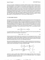
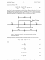
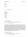
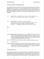
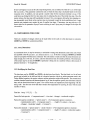
(averaged between the two grid points) and the uj’s superscripts (~, ~, and ~) are the total concentrations evaluated at the nodal points themselves (Figure 1). The term RY
is a function of the primary
species at the nodal point P. The spacings (dz)~, (dz)~, and AX are shown in Figure 1.
I
Ax
I
Control Volume
W
E
I-I
Figure 1: Discretization
grated finite differences.
Following the terminology
scheme for a one-dimensional
ofPatankar(1980),
problem using inte-
the discretized equations can be recast in the form
(44)
where
D.
(45)
aE = (dz).
D.
(46)
aw = (dz)w
-.”7,-.
.
-.
---~,’
~--,.w’
F,,,.,
____
,
. .
ap=CLE+(LM?
(47)
d = RPAx.
(48)
.-....- .-. ---
..:.–-
-12-
Steefel & Yabusaki
0S3DIGIMRT
Manual
3.4. Transport Algorithm in Global Implicit Approach
The addition of an advection term makes the set of partial differential equations much more difficult to
solve stably and accurately (e.g., Press et al., 1986; Patel et al., 1988), although the set of equations can
still be cast in the general form of Equation 44. One way to represent the first derivative which appears
in the advection term is to use a central difference method
uE– UW
au
2Ax
() % ~=
(49)
where the subscript P indicates that the derivative is evaluated at the nodal point P and AZ is 1)2(dz~ +
&zW). The truncation error for the central difference representation is said to be of the order AX2 because in the Taylor series expansion upon which it is based, only quadratic terms and higher are neglected
(Lapidus and Pinder, 1982). In contrast, a forward difference representation, given by
NJ
(-)
8X
has a truncation error of O(Z),
Despite the smaller truncation
stable for advectiondominant
vicinity of sharp concentration
Patel et al, 1988).
u.E– up
p =
(h).
(50)
‘
that is, all terms in the Taylor series higher than first order are truncated.
error of the central difference method, the method may not be numerically
problems because of the non–physical oscillations which can occur in the
fronts (Patankar, 1980; Daus and Frind, 1985; Frind and Germain, 1986;
It appears, therefore, that the numerical stability of a particular finite difference formulation for the first
derivative depends on the relative magnitudes of the advection and dispersiotidiffusion
terms. The relative importance of the two can be described by the dimensionless grid Peclet number
(51)
where AZ refers to the grid spacing at any particular point in space. Only for pe~,~d <2 is the central difference formulation unconditionally stable (Daus and Frind, 1985; Frind and Germain, 1986; Patel et al,
1988). The problem of stability can be “cured” by using a forward difference formulation written in terms
of the grid point itself(P) and the upstream or upwind node (Press et al., 1986). It should be pointed out,
however, that the upstream–weighted fo~ulation,
in addition to having a larger truncation error than the
central difference method, achieves its greater stability essential y by adding numerical dispersion (i.e.,
over and above the physical dispersion present in the problem). In a one-dimensional problem, however, numerical dispersion presents a problem only in tracking transient concentration fronts. The effect
does not appear in steady state one-dimensional systems (Patankar, 1980). Numerical dispersion can be
reduced by refining the grid in the vicinity of a sharp concentration front.
To take advantage of the greater accuracy of the central difference method at small values of pe~r~d, a
power law scheme proposed by Patankar (1980) is used. This method slides between a fully centered
fort-n at pe~,~d <2 to an upstream–weighted fo~ulation
at Pegrid > 10, where the upwind scheme is
necessary for stability. Using the power–law scheme of Patankar ( 1980), the finite difference coefficients
become
aE = De
o,
1
[lo, -Vell ,
(52)
+ Ilo,vwll ,
(53)
(
aw = Dw o,
1
(
-.r.
.. . ..
,,:,:
-.”..,--+.
~
<;~.
,.; .,.=<.=..-
o.lfkw
D.
I VW[ 5
)
?..,
0S3DIGIMRT
-13-
Manual
CJp= aE + aw,
Steefel & Yabusaki
(54)
where the operator IIA, B II means that the greater of the values A or 1? is used (equivalent to the FORTRAN operator AMAX1(A,B)) and I A [ refers to the absolute magnitude of the value. A fuller description may be found in Patankar (1980).
A fully implicit backward method is used to represent the time derivative (Lapidus and Pinder, 1982).
The equations to be solved for each component at each grid point at the (t+ At) time level are then
~
(U.j’’(t+ At) - Uj’’(t)) +apUf(t
+ At) - aEu~(t + At) - awU~(t
+ At) - Ryin(t + At)Az = O,
(55)
where At is the time step and (t) refers to the values at the present time level. As discussed above, the
equations are written in terms of the concentrations of the primary species in the code GIMRT (see Equation 32) and are expressed in terms of the total concentrations here in order to be concise.
3.5. Transport Algorithm in Operator Splitting Approach
3.5.1. Advection
When solutions require accurate resolution of concentration fronts in advection-dominant problems, highresolution shock-capturing techniques are often employed. These solution techniques are typically based
on explicit numerical schemes that are incompatible with a globally implicit solution of coupled transport and reactions (e.g., GIMRT). Decoupling (i.e., time splitting) the transport algorithm from the geochemical reaction algorithm relaxes the requirement for an implicit transport method, allowing the use
of high-resolution shock-capturing techniques based on explicit numerical schemes. The principal tradeoff for the additional accuracy is a strict limit on the ratio of time-step to grid spacing, a limit that is inherent in explicit transport methods. Typically, this limit becomes most restrictive under steady-state or
near steady-state conditions. (Note that steady-state does not mean static processes. In physical systems,
steady-state occurs when dynamic processes are balanced or fully compensating.)
In 0S3D, an explicit, third-order, total variation diminishing (TVD) numerical scheme (Gupta et al., 1991)
is used to model non-dispersive advective transport. The technique is based on calculating an estimated
concentration at the face of a grid cell that is dependent on the flow direction. In the case of flow in the
positive x-direction (i.e., u >0, the estimated concentration would be:
@l/2
a-1-l/2
(56)
“’+~(r)(c’+’~c’)
where
(57)
and
(58)
Similar calculations are performed for negative velocities and the method is generalized for multiple dimensions. The technique is third-order accurate in smooth regions, oscillation-free along concentration
fronts, and does not exhibit overcompression of fronts in the presence of physical dispersion.
-14-
Steefel & Yabusaki
3.5.2. Diffusion
0S3DlGIMRTMan
ual
and Dispersion
After the advection calculation, 0S3D proceeds to solve for diffision and dispersion. 0S3D assumes
that the principal direction of flow is aligned with the grid (i.e., D is a diagonal tensor). A centered numerical scheme, second-order accurate in space and time, is applied to the diffusion equation. The diffusionldispersion
(1995).
equations are solved with the WATSOLV sparse matrix solver of VanderKwaak et al.
The user should understand that parameterizations of hydrodynamic dispersion attempt to account for advection resulting from variations in the velocity field that cannot be resolved by the numerical grid. In
this standard representation based on Ficks law, dispersion is driven by the gradient of concentration and
parameterized by a linear proportionality constant (i.e., the diffusion coefficient). This is a gross simplification of a complex and poorly understood phenomenon. As such, the formulation neglects many features that have been observed in real systems. Principally, the user should be aware that unlike molecular
diffusion, dispersion is length and time scale- dependent.because of the inhomogeneity of the physical
media. As plumes start to spread, they are exposed to larger and larger scales of spatially variable material properties. Consequently, it is impossible to define dispersion parameters that are effective for all
time. Moreover, the magnitude of the dispersion parameter is dependent upon the grid resolution: larger
for large grid cells and smaller for small grid cells.
3.6. Solving the Equations
with Newton’s Method
As an example, consider a problem involving one-dimensional mukicomponent reactive transport. Equation 55 for any component j at the grid point P is a nonlinear function of the concentrations of the primary species at the the P grid cell in the case of 0S3D and of the P, E, and W nodal points in the case
of GIMRT. An iterative scheme, therefore, is required to solve the set of nonlinear equations in either
case. Both codes solve the nonlinear equations with Newton’s method which makes use of a Taylor series expansion to linearize the equations. Using Newton’s method, the linearized set of equations for the
ID global implicit case become
(59)
where jj is the discretized differential equation for the total concentration of each of the primary species.
In a 2D problem, one may have dependencies, of course, on other neighboring grid cells in the Y direction (i.e., north and south of the grid cell of interest). In the case of the operator splitting or sequential
iteration approach employed in OS3D, the Newton step only involves homogeneous and heterogeneous
reactions within the grid cell itself since the transport is handled separately (i.e., there are no nonlinear
terms involving spatial derivatives). The Jacobian matrix then takes the form
(60)
make Up the elements of the Jacobian submatrices.
The individual terms, t2fj/61CJI,
it follows that the Jacobian submatrices can be written further as
From Equation 55,
(61)
. ~.,
..,,
.w.
.
.
.
,.,
,,
.~
..-
-.
..,. . .
-’.: .,.. -- --
:-W’
, .. >..=
-.’
-?
,..
,.
,,.
. ..
y
.
q,::
-
-15-
0S3DlGlMRTManual
Steefel & Yabusakj
(62)
and
(63)
From Equation 12 and Equation 9, the partial derivatives of the total concentrations
primary species concentrations are (Lichtner, 1992)
with respect to the
where 1 is the ionic strength, the subscript z refers to the secondary species, and k is a (second) dummy
subscript referring to the primary species. The partial derivatives of the reactions rates are given by
(65)
where any dependence of the rate law on the activities of species far from equilibrium has been neglected
and only first order reactions are considered (M and n = 1). For the case where the activities of various
species (e.g., H+) affect the far from equilibrium dissolution rate, additional terms appear in the partial
derivatives (not given here). The partial derivatives of the ionic strength, 1, with respect to the primary
species can be written as (Lichtner, 1992)
(66)
and the derivatives of the activity coefficients with respect to the ionic strength are
dlog~k
—
dI
Az:
=—
(67)
~+b.
21112( 1 + ~ & 1112
(
)
If we define j~ as making up the elements of the vector b when taken over all of the grid points in the
system and the i?jjf aCjl as forming the elements of the global Jacobian matrix A, then Equation 59 can
be written in the familiar form
A.6C=b.
Once the 6Cj/ are computed, they are used to update the concentrations
C;’w= Cy+dcy
(68)
of the primary species
(j’ = 1,... ,Nc x M).
This completes a single Newton iteration. The procedure is repeated until convergence
residuals (the j~’s) are reduced to a tolerance set in the code, i.e.,
f3 z o.
(69)
of the function
(70)
Without basis switching, it maybe necessary to use the logarithms of the concentrations since the concentration of a basis species (especially in the case of redox) may drop to a very small value. If the logarithms
of the concentrations are used, it is still possible to solve such problems without basis switching, although
.-.
: .{, ,, ..--?-
:*’,:
“.?---
- :
,,~
$: ~-=~.--
... ,
0S3DIGIMRT
-16-
Steefel & Yabusaki
Manual
in redox systems the code sometimes reduces the time steps many times in order to obtain convergence.
In both 0S3D and GIMRT, the logarithms of the concentrations are solved for if no basis switching is
used and the linear concentrations are used if full basis switching every Newton iteration is used. The user
should normally begin by running the codes without basis switching, since that will be faster if there are
no non-convergences of the Newton iteration. If the code is either not converging within the maximum
number of Newton iterations, then full basis switching should be tried. The user may also want to compare the iteration count with and without basis switching, since the bottom line is the total CPU required
to solve a particular problem.
3.7. Structure
of the Jacobian
Matrix
It is instructive to examine the structure of the Jacobian matrix which arises from the discretization of the
coupled reaction–transport equations, since it has a bearing on the choice of a method to solve the set of
linear equations given by Equation 32. The Jacobian matrices exhibit a block rridiagorud structure in a
one-dimensional system. The blocks making up the global matrix A are NC by IVCsubmatrices corresponding to the primary species at any grid point. That is, if we are writing the conservation equation for
siOz,aq at a particular point in space, the equation .fSioz,., will be differentiated with respect to all NC
primary species (e.g., S’i02,~~,”Al ‘++, K+, etc.). As an example, consider a one-dimensional system
described by 4 primary species which is discretized using 4 grid points (this is for illustrative purposes
only, since hopefilly one would not attempt to solve differential equations using only 4 grid points). The
matrix A can be represented compactly as a series of 4 x 4 submatrices, A331,such that
A=
A21
~
1
00
A22
A32
A23
A33
A43
O
A34
“
A44 1
(71)
Those readers with some familiarity with numerical methods will recognize that this is the structure of
any finite difference formulation of a partial differential equation (e.g., the temperature equation), except
that in this case the entries are submatrices rather than single coefficients. If we reduced the system to a
single chemical component, then the forms of the temperature and reaction–transport matrices would be
identical. The submatrices need not be filled entirely with non–zero elements, but, in general, they will
be dense in systems with either a Iarge number of mineraIs or a great deal of complexation. The diagonal
submatrices (All, A2Z etc.) contain contributions from both the heterogeneous reaction term, R~,
and
from the total soluble concentrations (the Uj’s). The offdiagonal submatrices, in contrast, contain only
contributions from the total soluble concentrations at the neighboring grid points. Note that the global
matrix A is sparse (i.e., the ratio of zero to non–zero entries in the matrix is large) when the number of
grid points is large (e.g., greater than 100), even though the submatrices (reflecting the coupling between
the various species due to reactions) may themselves be fairly dense.
Any method used to solve the set of equations described by Equation 59 which arise in the case of the
global implicit method should take into account both the sparseness of the Jacobian matrix A. In the code
GIMRT, the equations are solved now using the WATSOLV package (VanderKwaak et al., 1995). In the
WATSOLV package, one may use either the GMRES algorithm or the CGSTAB algorithm developed by
the authors. Users should consult the manual prepared by these authors (VanderKwaak et al., 1995) on
the various input options which can be specified. At the present time, all of these input options are in
data statements at the beginning of the driver routine gimrt.
f. We have found, however, that for redox
problems (and probably any similar problem in which there is a large range of concentrations) that the
convergence criteria need to be set much smaller than indicated by VanderKwaak et al. (1995) in their
manual. We found that the Newton iterations failed to converge when the tolerance was too loose and a
Steefel & Yabusaki
-17-
0S3D/GIMRTManual
level of preconditioning equal to O was used (see the WATSOLV manual). This could be remedied by
either setting the level of preconditioning to 2 or 3 or by simply tightening up considerably the tolerance
and using a level of O. This second option appears to give the best results.
3.8. Convergence
Criteria
Convergence is obtained where all of the function residuals have been reduced below a tolerance set by
the parameters at ol and rt 01 in the driver routine gimrt.
f and in the file newton.
f in the case of
the code 0S3D. These parameters are located in data statements at the top of the named routines. The
tolerance on function residuals is computed from
tolmaz
= atol + rtol (Cj) ,
(72)
where C’j refers to the primary species concentrations. If they are changed, the code should be recompiled. The functions residuals, when multiplied by the timestep delt
in order to compare to the tolerances at 01 and rt 01, have units of moles per m3 bulk volume. The default setting for the absolute
tolerance is 10–9 mole m–3 which corresponds to 10–12 mole liter– 1. Convergence will also be obtained
where either the absolute value of the log concentration correction or the linear concentration correction
drops below 10–15 (i.e., approaching the roundoff error of the computer).
3.9. Updating
Mineral
Properties
When convergence is achieved, the mineral volumes and surface areas (and porosity, if desired) are updated. The individual mineral volume fractions, ~~, are updated with the expression
c#Jnt(~
+ At) = An(t)+
hr~(t
+
At)At,
(73)
where Vm is molar volume of the mineral and rm is its reaction rate. The user may either choose to leave
the porosity constant (in which case its value is determined by the user in the input file), or the user may
choose to update the porosity. Where updated, the porosity is computed from the
(74)
4=1-~&.
k=]
Note that in this formulation, both mineral volume fractions and reactive surfaces are assumed constant
for any one time step. This decoupled, two step approach normally works well since the volume fractions of the minerals usually evolve much more slowly than the solute concentrations. However, in certain cases, the approach may lead to inaccurate solutions. The code has a check to make sure that the
volume fractions of a dissolving phase does not go below zero, in which case a mass balance error would
occur. Where the code indicates that this is occurring frequently, the time step should be reduced. In addition, one can specify a maximum rate of increase (using the parameter vpptmax
described below) or
decrease (using the parameter vdis smax described below) of the mineral volume fractions. The two
step approach employed here may require smaller time steps when either the dissolving or precipitating
phase has a high volubility or where very little of it is present. Where only small amounts of a mineral
are present, than it is possible that dissolution of the entire amount present within a grid volume may occur in a single time step. This typically results in either inaccurate propagation of a mineral front or in
oscillations in the mineral volume fraction profile.
-18-
Steefel & Yabusaki
0S3D/GIMRTMan
ual
Initial reactive surface areas are specified along with initial mineral volume fractions by the user at startup.
Reactive surface areas of minerals are updated differently at the present time depending on whether the
minerals are primary or secondary. For primary minerals, the surface areas are given by
[(*)
Am = Am,o
{
(*)]’”
‘j’
.&
[1
‘is’”zu’i”n
)
precipitation
(75)
}
where +m,o is the initial volume fraction of the mineral m and @O is the initial porosity of the medium.
This formulation ensures that as the volume fraction, @~, of a mineral + O, its surface area also ~ O. In
addition, for both dissolving and precipitating minerals the term (@/@. )2’3 requires that the surface area
of a mineral in contact with fluid ~ O when the porosity of the medium ~ O. For secondary minerals
(i.e., those initially with a volume fraction= O), the reactive surface areas as a function of time are given
by
2/3
Am = Am,O
[($);]
dissolution
?
&
[1
precipitation
(76)
1
which implies that if a secondary were to begin to dissolve, its surface area would equal its “initial” surface
area, Am,o, when Vm = 1 (if the porosity were constant).
4. PROGRAM
STRUCTURE
4.1. Global Implicit
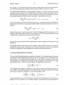
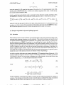
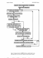
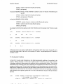
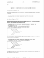
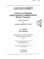
The basic structure of the global implicit approach (GIMRT) is summarized in Figure 2. After specifying
the initial and boundary conditions, the code begins stepping through time. Whhin each time step, a series of Newton iterations is required because of the nonlinearity of the equations. Each Newton iteration
consists of calculating the function residuals (the ~~’s given by Equation 55) and the partial derivatives
of these functions (the Jacobian elements) with respect to the unknown concentrations (Equation 59) and
then assembling and solving the linear set of IVc x Al algebraic equations in order to obtain the corrections to the component concentrations. If the basis switching option is turned on, then the code checks that
the basis species chosen are those that form a linearly independent set and that are present in the greatest
concentration.
If more concentrated species are present than those currently used for the primary species, then a basis
switch is carried out at the appropriate grid cell (i.e., the reactions are rewritten in terms of a new set of
primary species). Unlike the operator splitting approach in 0S3D, the residual functions and the Jacobian
matrix are computed over the entire spatial domain before solving a global system of linearized equations.
Once convergence is achieved, the mineral volume fractions and mineral surface areas are updated. If the
reaction–transport calculations are combined with a calculation of the flow and temperature field, these
would normally be updated as well at this time. At the end of each time step, an algorithm which computes the second derivative of the solute concentrations with respect to time is used to determine whether
the time step should be increased or decreased. This algorithm provides a way of minimizing the time
truncation error (if that is an issue in a particular problem) and also of controlling the size of the time step
so as to maintain numerical stability.
The program structure for the time splitting (operator splitting and sequential iteration) method is similar,
differing primarily in the fact that the transport is carried out in advance of any calculations of the reactions
,,
,
,7
-,*-,-
.
,.
. .. . . . . . . . . ..
,
<’;,s , ‘:??=---- “-
-: ~---.
--
-,,.,:-..-,
0S3D/GIMRTManual
-19-
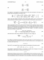
Steefel & Yabusaki
(Figure 3). The reaction calculations are then calculated individually at each point in space. Since these
reactions are not directly coupled via transport to the reactions in neighboring cells, the calculations can
be carried out independently. The size of the system of equations to be solved at each grid point is then
NC by N. and there is no need to assemble the global system of function residuals and the global Jacobian
matrix over the entire spatial domain. The sequential iteration method differs in that 1/2 of the reaction
rate is included as a source term in advance of the “reaction module” and so iteration between transport
and reaction is required to achieve convergence (Figure 3). Mineral volume fractions and the porosity are
updated ajler all of the species have been reacted at all the space points, in a similar fashion to the global
implicit.
5. FEATURES
OF THE CODE
Before running the code, the user of OS3D and GIMRT needs to decide what physical process
he or
she wants to model and design the simulation accordingly. This involves choosing the boundary conditions for the problem (e.g., no flux boundaries or fixed concentration boundaries) and setting up the initial
grid andlor initial mineral zones. The user must decide how many grid points are needed to solve a particular problem. Typically one proceeds by carrying out the simulations on a relatively coarse grid (e.g.,
30 to 50 grid points) and only refining the grid later when one has a general idea of the behavior of the
system. The user also needs to decide what level of chemical complexity they wish to consider. This can
involve choices in the number of independent components (primary species), the number of secondary
species, and the number of reacting minerals. The discussion in the sections which follow is designed to
make the basis for these decisions clearer. These sections are then followed by a step by step discussion
of the input file threedin
which is needed to run OS3D and GIMRT.
5.1. Units
Although there are some advantages to allowing the input of data in any self-consistent set of units, many
of the parameters used in GIMRT and 0S3D are given commonly in certain units, so we have decided
to require these units. All units for input parameters (e.g., velocities, reaction rates etc.) are given in the
description of the input file threedin.
All distances are in meters. The code assumes that the reaction
rates for minerals are in units of mol m– 2 s ‘1 (these are converted in the code to mol m–2 yr-l. Diffusion
coefficients are in units of m ‘2 s– 1. All other references to time (time for plot files, timesteps etc.) are in
years. Velocities, for example, are in units of m yr- 1. Concentrations for aqueous species are in units of
mol kg–l water (i.e., molality). The partial pressure of gases are specified in bars.
5.2. Boundary Conditions
At the present time there are three possible boundary conditions which can be used in GIMRT and 0S3D.
The most straightforward way to describe the possible boundary conditions in the codes is to actually
begin with the thirdtype of boundary (also sometimes called a Danckwerts boundary conditon). This is
a boundary condition which requires continuity of flux across the boundary. Both codes assume that the
flux at these boundaries is purely advective (i.e., no diffusion or dispersion occurs upstream). Where the
flow is into the system, the flux at the first interior nodes downstream is assumed to be just uCeZt, the
same as the advective flux at the upstream, exterior node. In this special case where the dispersive and
diffusive flux are neglected, the third type of boundary condition is the same as a Dirichlet or fixed
-20-
Steefel & Yabusaki
]Specifv
0S3DlGlMRTManual
initial and boundarv
[Begin time stepping
lCalculate concentrations
secondarv~
condition~
[
of~
I
Calculate
total concentrations
w
y=-
Calculate derivatives of
total concentrations
and
reaction rates with respect
to primarv species
Solve linear set of equations
for concentration
corrections
w
I Check for converqencel
Yes
I Update mineral volumes
and areas
>
w
lTransient
temperature
and flow field?l
I
No
Yes
Figure 2: Program structure for GIMRT which uses a global implicit or onestep method used to solve the multi-component reaction-transport equation.
,-,.
? .”7 .,
,.
.
,
-.?
—-..
,.
.
.
.
.
,.m
...
-
-.
-.
n,,?---—-
-~
,....-,_ . .
-.
I
OS3DlG~RT
Steefel & Yabusaki
-21-
Manual
Specify initial and boundary conditions
IBegin time stepping
I
—-
.—
.
..-
u
lAdvect all species using ‘NW algorithml1
IDiffuse and/or disperse speciesl
lSequential Iteration!
~dd source term I
v
Reaction at individual space points
Calculate secondary species concentrations
Calculate total concentrations
Calculate mineral reaction rates
Calculate Jacobian matrix
Solve system of equations
Update concentrations until converged
&
v
Sequential Iteration?
I
~
Yes
Update mineral volume fractions
Figure 3: Program structure for 0S3D which uses time splitting of the transport
and reaction step or a sequential iteration between transport and reaction.
concentration boundary condition. At the boundary nodes where the flow passes out of the domain the flux
is also assumed to be purely advective, so that it passes out of the system with the downstream, exterior
node having no effect on the system. Note that when the flow across a boundary is non-zero, we always
assume that the dispersive and difisive fluxes are equal to zero.
.---- ,.
,,
------
“
/.
.
-Y-----
--
.
.-
-e--l
-or------
.-.7,--
-.
OS3DlGIMRTMan
-22-
Steefel & Yabusaki
ual
The second type of boundary condition is the no-flux condition which is applied when there is no flow
across the boundary. In this case, both the advective flux and the dispersive/diffusive fluxes are equal to
zero.
The last type (often called thefir.st type or a Dirichlet boundary condition) is normally applied when the advective flux is equal to zero but there is a dispersive or diffusive flux across the boundary (if the advective
flux is non-zero, then the code automatically assumes a zero dispersiveidiffusive flux). This condition is
many cases is not physically reasonable, since it assumes that the diffusive andor dispersive flux through
the boundary does not affect the concentration of the exterior node (i.e., it is fixed). This boundary condition would normally be applied where the physical processes exterior to the domain are such that the
diffusiveldispersive flux through the boundary is not enough to alter the concentrations there. One example might be a boundary along a fracture within which the flow is so rapid that the diffusive flux through
the fracture wall has a negligible effect (e.g., Steefel and Lichtner, 1994). Another example might be a
boundary corresponding to an air-water interface where a gas like Oz or C02 is present in such large abundance that it effectively buffers the concentrations in the aqueous phase. Another example which is often
mentioned in this regard is the case where mineral equilibria fixes the concentrations. This is dangerous,
however, since the system is only completely determined in the special case where the phase equilibria
results in an invariant point, i.e., no thermodynamic degrees of freedom exist. This is extremely rare in
open systems, despite the frequent invocation of this condition in metamorphic petrology. Normally, since
the concentrations will not be uniquely determined, a rigorous treatment would require that a speciation
calculation with equilibrium constraints be carried out to actually determine what the concentrations at
the exterior node should be. This, however, is not implemented at the present time.
0S3D and GIMRT differ slightly in their application of a Dirichlet boundary condition where the advective flux across the boundary is zero. In the case of GIMRT, the user may specify that an exterior node
be a fixed concentration node and that it affect the interior node (i.e., there will be a non-zero diffusive
and/or dispersive flux through the boundary). In 0S3D, however, the code always assumes the dispersive/diffusive flux across the boundary is zero (due to the way the transport algorithm is formulated). If
one wants to use a Dirichlet condition in the case of 0S3D, one does so by fixing the concentrations at the
first node or nodes interior to the boundary. This will have the same effect as allowing an exterior node
influence the interior domain, except that one can think of the boundary as having been moved inward
by one grid cell. The procedure for doing this is described in the section below explaining the input file
threedin.
To summarize the boundary condition options in 0S3D and GIMRT, a non-zero flow across the boundary
means that the code will use the upstream, exterior boundary concentrations to give a purely advective
flux at the boundary and the code will allow a fluid packet to pass out of the system with no influence
from a downstream, exterior nodes. Exterior nodes across a boundary through which there is no flow will
not influence the interior domain, unless the Dirichlet boundary condition option is used (usage described
below). The default is therefore no diffusiveldispersive flux boundaries which is only overridden where
the Dirichlet option is invoked.
5.3. Choice of Primary and Secondary Species
After setting up the problem physically, one needs to decide on the chemistry to be included. The method
for specifying primary and secondary species is essentially that devised by Peter Lichtner for the code
MPATH. The codes 0S3D and GIMRT require that one specify an initial choice of primary species
which then determine the number of independent chemical components in the system. This choice of primary species is not unique, however, as discussed in the section 2.2. By making use of the basis switching
,-, .,..
.,
,,-,
!
-Tx?-?----?wr-
i:..::
.-,..... “.
,
.::
.-/n--
7
..-
, ,.-,
-
,.
OS3DIGIMRT
Steefel & Yabusaki
-23-
Manual
option, it is possible to allow the code to dynamically choose the set of primary species to be used in writing the reactions at each grid point (see discussion below). Unlike EQ3/EQ6 (Wolery et al., 1990), for
instance, the user must choose which secondary species are to be included in the simulation. This can be
an advantage for multicomponent reaction–transport modeling since one would like the option of carrying
out chemically simplified simulations. However, the user must take care that important species are not
neglected. Future versions of the code will have the capability of reading all of the potentially relevant
species from the database.
The only cautionary note here is that one must include either among the primary or secondary species a
species which is used in writing the reaction in the EQ3fEQ6 database. Note that this database is provided
with the code in a reformatted form. For example, if one wants to include aluminum in the simulation, then
the species A1+3 must appear among either the primary or secondary species since that species is used
as the primary or basis species in the EQ31EQ6 data base. In the same way, one must include C0z(9)
among the list of gases if carbon is to be present in the system. If this is not done, the code will not be
able to find the reaction when searching the data base. One should not, however, include any secondary
species which cannot be written completely in terms of the basis species specified in the input file. The
simplest way to grasp these features is to check the database to see which species are used to write the
reactions involving a species of interest.
The species HzO presents a special case since in many cases it is present in such abundance that its activity can be taken as unity. If one wants the activity of HzO to be 1, then it should be left out of the
list of primary and secondary species. The code will still balance the reactions properly as if H20 were
- present. If, on the other hand, one wants to carry out a mass balance on HzO, then it should be included
in the list of primary species and it will be treated like any other species, except for the treatment of its
activity coefficient. OS3D and GIMRT assume that the activity of HzO is given by its mole fraction in
the solution.
5.4. Redox Reactions
There are many possibilities for choices of primary and secondary species to represent redox reactions.
Both 0S3D and GIMRT write all redox reactions as whole cell reactions, i.e., electrons are not used as
either primary or secondary species. It is easy to show that the electrons are completely unnecessary if the
solutions are electrically neutral, and the inclusion of electrons requires that one include a species the mass
of which should everywhere be zero. With the whole cell reactions, no special provision for redox species
and reactions is necessary, (in contrast to statements by Yeh and Tripathi (1989)) although the inclusion
of redox reactions implies that we have included an additional mass balance equation representing the
conservation of exchangeable charge.
Since 02(g) is used as the basis species in redox reactions in the EQ3/EQ6 data base, it must be included
in the list of gases in the input file if redox reactions are to be considered. A gas, however, cannot be used
as a primary species in 0S3D and GIMRT since gases are not included in the mass balances. One could
use 02(ag), however, or any number of other species which form a redox couple, for example, f’e+2 and
Fe+3, or HS– and SO: 2. When using the basis switching option, the initial choice of primary species
to represent a redox couple may not be important since the code will automatically write the reactions at
any particular grid point in terms of the dominant redox couple, i.e., that which is present in the largest
concentration (see section on Basis Switching below). This maybe particularly useful for redox problems
which can show convergence problems (this approach works best where basis switching is carried out
every Newton iteration). The user may choose not to use basis switching at all, to use it at the beginning
of every timestep, or to use it every Newton iteration. The same proviso, however, applies about including
.-..
r-
,,.
--
---
‘- -
...,,.‘7=-
.,
..
-—..-
~-
.
.
.
. . .
-24-
SteefeJ & Yabusaki ,
OS3D/GIMRT
the species which are used as basis species in the EQ3/EQ6
5.5. Acid-Base
Manual
data base.
Reactions
Acid–base reactions require no special treatment other than in the initialization
process where one nor-
mally fixes or calculates pH rather than an H+ concentration. Once a pH has been either fixed or calculated
in the initialization procedure, however, H+ can be treated like any other component. Again, no special
considerations are needed in contrast to the statements by Yeh and Tripathi (1989).
5.6. Basis Switching
As discussed above, both 0S3D and GIMRT can rewrite the reactions in terms of the most concentrated
set of linearly independent species. This is not absolutely necessary if one is solving for the logarithms of
the concentrations, but basis switching, when carried out every Newton iteration, does appear to reduce
the number of times the Newton fails to converge, particularly in the case of redox problems. If full basis
switching is used (every Newton iteration), it should not be necessary to solve for the logarithms of the
concentrations and one can make use of standard relaxation techniques to reduce the size of the Newton
step when the linear concentrations are employed. The code carries out basis switching by first sorting the
species concentrations in order of abundance and then systematically attempting to construct a linearly independent set from those concentrations (see the subroutine switch.
f). The recommended procedure
is to try to run the problem without basis switching, since that will be the fastest method if the code converges properly. If numerous non-convergences occur, however, we recommend trying basis switching.
The various input parameters required to turn the option on and off and to set the maximum allowable
concentration correction limits are described in detail in the section on the input file threedin.
5.7. Activity Coefficient Model
At this time, the user may choose to run the code either with unit activity coefficients or with an extended
Debye–Huckel formulation to calculate activity coefficients for the. ionic species. The Debye–Hiickel
formulation is given by
log ‘y~= –
AZ: (1)1/2
+ bI
(77)
1 + B & (1)1/2
The coefficients for the temperature dependence of the parameters are taken from the EQ3 data base,
5.8. Initialization
Procedure
The codes GIMRT and OS3D initialize the solute concentrations at individual grid points over the domain by carrying out a distribution of species using a number of options. The initial concentrations of the
primary species may be determined by
●
carrying out a mass balance on a total concentration
(e.g., aluminum),
. carrying out a charge balance on a species (e.g., Cl– ),
Steefel & Yabusaki
-25-
0S3D/GIMRTManual
. a mineral equilibrium constraint (e.g., 11+ required to be in equilibrium
with calcite),
. fixing the activity or partial pressure of a gas (e.g., COZ(9)),
●
fixing the activity (e.g., pH) of a species,
●
fixing the concentration
●
fixing the number of moles surface hydroxyl sites per mole mineral and the intrinsic surface area
of the mineral (i.e., m2/g).
of a species, and
This last option is available in 0S3D and GIMRT and it allows one to specify the concentration of surface
complexes. These are specified by giving a site density (mole per m2 mineral) and a surface area of mineral per gram mineral. The total concentration of surface hydroxyls developed on the mineral (converted
to mol/kg solvent) is then computed from this information and the abundance of the mineral specified in
the startup file. If a mineral is initially is not present but one would like to consider adsorption on this
mineral, then the total concentration of surface hydroxyls on this mineral is set to a small number ( 10– 1°
mol/kg) and its concentration only builds up once the secondary mineral precipitates.
How each of the above initialization
threedin
below.
5.9. Temperature
constraints is applied is described in the section on the input file
Gradients
Since GIMRT and 0S3D are based on finite difference methods, they have no problem handling temperatures which are non-constant either in time or in space, although this option has been implemented
only in GIMRT due to time constraints on the preparation of the software. If either a non-default thermodynamic data base or the master25.
dat a data base is not used at startup, then the code defaults
to the rnas t ert emp. dat a file where equilibrium constants are given at temperatures of O“C, 25*C,
60°C, 10O”C, 150”C, 200°C, 250”C, and 300*C at pressures corresponding to the water saturation curve.
The code then fits a polynomial to the thermodynamic data so that equilibrium constants can be generated
at any temperature between O°C and 300° C along the water saturation curve. Simulations are possible at
other pressures and temperatures, but the user must provide his or her own database in the same format as
mast er25 . data or mas t ert emp. data. In addition, the algorithm for fluid density must be modified as well. Presently the fluid density is calculated as a function of temperature from a polynomial fit to
the data in Helgeson and Kirkham (1974). Fluid viscosity is calculated from the data presented by Bruges
and others (1966).
A temperature dependence is also included in the calculation of the reaction rate constants (Equation 29),
the diffusion coefficients, and the fluid densities. Reaction rate constants at temperature are obtained normally by extrapolating the rate constants for 25° C given in the input file t hre ed in. If one would rather
input directly the desired rate constant at temperature, than the simplest procedure (short of changing the
source code) is to input the rate as if it were the 25° C data while changing the activation energy to O
kcal/mole. There is also an option for directly inputting the diffusion coefficient at temperature.
There are two options for temperature presently implemented in GJMRT. The first is simply to run the
simulation isothermal y, either at 25° C or at temperature. The second is to specify a linear temperature
gradient which operates only in the X direction. Many other ways of handling temperature are possible,
including allowing for a transient temperature field, but this must be provided by the user/programmer at
the present time. This can be done with a simple read of temperatures, making sure that the dimensions
~ .-.. ,
- ---- ?w-,
-..’
,
.-. , :,.,
:7”,.-,
-:-.
,
. .. . ....
---
-..
. . . ..
.-
-26-
Steefel & Yabusaki
0S3DIG1MRT
Manual
of the temperature field match those specified in the code. The positions in the code where a user should
place a routine for calculating or inputting a temperature are marked in the routine gimrt.
f.
5.10. Updating Porosity and the Transport Coefficients
A user can choose at runtime whether to include a feedback between the changes in the volume fractions
of the various minerals in the system and the diffusion coefficient. In the present version of the code, there
is no provision for a feedback between porosity and permeability. This is planned as a feature of the next
release. To do so requires that one solve the continuity equation (the equation for the conservation of fluid
mass) in addition to the reaction–transport equation (Steefel and Lasaga, 1990; Steefel and Lasaga, 1994).
Local changes in the porosity result normally in local changes in the permeability, thus causing a change
in the distribution of the hydraulic head (or fluid pressure). The continuity equation should be solved in
a one-dimensional system with constant head boundary conditions, and not constant flux conditions as
was done in Bemer (1980). The fluid velocity becomes infinite as the porosity ~ O when the constant
flux conditions are used.
If the user decides to update porosity during the course of the simulation, then the magnitude of the diffision coefficient in the porous medium, D*, changes according to Archie’s Law (Dullien, 1979)
(78)
where m is again the “cementation exponent” in Archie’s Law. This formulation ensures that D* ~ O as
@~ O. It should also ensure that the porosity will not go negative if the chemical reactions are driven by
mass transport since the porous medium locally becomes a closed system.
6. INSTALLATION
The codes OS3D and GIMRT are designed at the present time to be installed and run on UNIX systems.
The code has been tested to date on Sun, Digital (ULTRIX), Silicon Graphics, and IBM RS-6000 series
UNIX-based workstations. A number of suggestions follow which are designed to make it easier to customize the installation.
The directories GIMRT and 0s3 D contain the subdirectories
src,
where the source files, Make f i-1 e, and include files are located,
database,
cated,
dot,
where the default data bases, master25
where the documentation
. data
and master
temp.
data
are lo-
in the form of a PostScript file is located.
The user needs to modify the source code so that the correct address of the GIMRT or 0S3D directory tree
can be found. The address of the data bases is specified in the file database.
f in the lines
c
;
open appropriate
data
base
file
i.f (datal.
ne. ‘ ‘ ) then
open (iuni. t5, file= datal,
status=’
-.syy
t.
.. ..
,,
.
r
. .
-,
. ..
--------
7,-,
..
.
.
+
. . . .
., ,.*,
.
.
;.,
TJ~:-
-,
-
,nT.”
old’
—-, ” = -
, err=334)
~..
OS3D/GLMRT
Manual
-27-
–-> using
database:
(*, ’(”
else
if
(temp
.eq.
25. dO) then
open ( iunit5,
file=’/home/steefel/GIMRT/database/master25
.
status=’old’
,err=334)
-->
using
data
base:
write(*,
*) ‘
else
open(iunit5,
file='/home/steefel/GI~T/database/mastertemp.data'
status=’old’
,err=334)
.
--> using
data
base:
write(*,
*) ‘
write
endi
Steefel & Yabusaki
‘ ‘ ,a)
‘ ) datal
data’,
master25’
,
mastertemp’
f
One of the options above involves a non-default database
which is discussed inthe sectionon input files below.
or location (specified bydatal.ne.’
)
The sourcecodecomes
with MakefilesMakegimrt
andMakeos3dwhich
should remodified slightly
depending onthe particular operating system to beused. Copy the FileMaker imrtorMakeo
s3d-over
toMakefile
anduncomment
the lines appropriate forthe particular system on which the softwareis
being installed (e.g., Sun, DEC, or IBM). These options at this time involve only slight differences in the
compilation flags, mdinthe
case of the~MAIX
operating system, thecommand toinvoke the FORTRAN compiler.
The second file which may have to be modified before compilation is params.
inc in the case of the
GIMRT code or params.os.
inc in the case of the 0S3D code. This file contains the parameter statements which dimension the various arrays in the codes. The codes are set up so that at run-time the dimensions of the arrays are checked to make sure they are sufficiently large. If the user needs to increase
the dimension of the arrays or wants to decrease them so that they are just large enough, the following
parameters can be changed
●
zncomp, 1 plus the number of independent chemical components in thes ystem (specified in t hreedin),
●
WV-CL
1 plus the number of reacting minerals in the system (specified in t hreedin),
●
nzspec, 1 plus the number of secondary species in the system (specified in t hre ed in),
●
nzgas 1 plus the number of gases in the system (specified in threedin),
●
mx, my, nzz, the number of grid points in the X, Y, and Z directions respectively used to solve the
for the solute concentrations (specified in threedin).
and
If the file params.
inc or params_os.
inc are modified, then all of the subroutines which include
this file are recompiled when Make f i 1 e is run again.
When the appropriate changes have been made, the source code can be compiled and an executable image
can be created. This is done by giving the command make which runs the default file Makef i 1 e.
So as to avoid the necessity of creating multiple copies of the executable image, one normally creates a
symbolic link to the user’s bin directory. This allows the code to be run from any directory chosen by
the user (assuming the input file threedin
is located there). This can be done by moving to the user’s
bin directory with the command
cd - /bin
-28-
Steefel & Yabusaki
0S3D/GIMRT
Manual
where N indicates the user’s home directory, and then typing
in – s N /path/gimrt
gimrt
followed by
rehash
to update the hash table so that the symbolic link is recognized. The designation /path
refers to the location of the executable image (e.g., N/ GIMRT). The user should also make sure that the /bin directory
is included in their search path (generally in the . c shrc or . login
file). The search path is set with
the command set
path.
7. RUNNING
GIMRT
and OS3D
OS3D and GIMRT both read the user–provided input file threedin
on startup in addition to a file
containing the thermodynamic data base. The file t hreedin
includes various control parameters and
physical parameters which are necessay in order to run the code. The file also includes information on
the initial and boundary conditions, the minerals and species to be included, and the rate data to be used in
the simulation. The input is organized as a series of cards which include comment lines followed by the
fields where the user inputs data. Comment lines begin all cards which are numbered. Input data begins
on the second line after the last comment line (i.e., comments and input are separated by one space).
7.1. Control Parameters
Control and physical parameters for the simulation are specified in Cards 1 through 7 of the input file
threedin.
A typical example is given below.
* THIS IS THE INPUT
-------------------(1)
‘ Short
(2)
title
(up
Course
Test
database
to
80
data
TO GIMRT AND 0S3D*
——
—___________
for
default)
characters)
Problem’
( 1 blank
space
II
(3)
tstep
0.005
1.e-06
(4)
jpor,
o
0.1
(5)
j temp,
.- ,
,,. —.,
(max.
delt)
, delt
(initial
0
5.d-03
0.01
cons tantpor
0.01
tinit,
(porosity)
0.001
tgrad
delt)
, vdissmax,
,
ttol,
vpptmax
ijacob,
bpeg
-29-
0S3D/GLMRTManual
o
25.0
0.0
master,
(6)
/h+,
2
(7)
nstop,
1 3.0
20.0
Steefel & Yabusaki
iswitch,
igamma
2
(prtint
30.0
(i),
40.0
i=l.
..nstop)
50.0
. Card (l) LTITLE Title of simulation (up to 80 characters) enclosed in single quotes.
●
Card (2) DATA 1 String (up to 100 characters) with location of a user–provided thermodynamic data
base. If no location is provided (i.e, the code reads ‘ ‘), then the code defaults to either
mast er25. data if the input temperature (given below) is 25° C or to mas t ert emp. data
if another temperature is given.
●
Card (3) TSTEP, DELT, TTOL, IJACOB, BPEG
TSTEP:
maximum time step in years allowed.
DELT
initial time step in years.
lTOL:
parameter controlling the tolerance on increasing the size of the time step. Making
t t 01 smaller decreases the rate at which the time step is increased, for the purpose
of controlling either the time truncation error or for numerical stability.
IJACOB:
flag controlling update of Jacobian
O – update Jacobian every Newton iteration
1
BPEG:
●
– when del t = 1/2 ts t ep, update Jacobian every 3 Newton iterations and
when del t = ts t ep, update Jacobian every 6 iterations.
maximum change in molality in any one Newton iteration. Reducing bpeg increases the under-relaxation of the Newton step and may sometimes prevent nonconvergence, although the total number of iterations required may actually increase.
Card (4) JPOR, CONSTANTPOR,
VDISSMAX,
VPPTMAX
JPOR: flag controlling update of porosity and flow
O – no update of porosity.
1
– porosity is updated.
CONSTANTPOR:
porosity of the medium for the case where the porosity is not updated
(jpor = O). If jpor = O, the porosity is taken from cons t antpor
rather than from
the sum of the volume fractions of the minerals in the system. If jpor = 1 (porosity
updated), cons t antpor
is ignored.
VDISSMAX: maximum rate of decrease of a mineral’s volume fraction (units of yr-l ).
Can be used to limit the amount of mineral dissolution which can occur within a
single time step. Useful where either the dissolving phase is very soluble or where
very small amounts are present. Where very small amounts of a mineral are present,
inaccurate mineral front propagation may occur where most or all of the mineral
present within a grid volume dissolves in a single time step.
,,-
.-
..>. =
.-,-7
-----—.
,,
.,.
–--”.—.——
..
..-
------
.
.
-.
-30-
Steefel & Yabusaki
VPPTMAX:
●
0S3D/Glh4RTManual
maximum rate of increase of a mineral’s volume fraction (units of yr- 1).
Card (5) JTEMP, TINIT, TGRAD
JTEMP:
flag controlling temperature option.
O – isothermal.
1
●
– linear temperature gradient operating only in X direction.
TINI17
temperature in “C at grid point 1.
TGRAD:
temperature gradient in ‘C m– 1. A positive gradient causes the temperature to
increase from grid point 1, a negative gradient causes it to decrease.
Card (6) MASTER, ISWITCH, IGAMMA
MASTER:
string (up to 18 characters) enclosed in single quotes specifying master variable
(used in controlling time step).
ISWITCH:
flag controlling basis switching.
O – no basis switching (solves for logarithms of concentrations).
IGAMMA:
1
– not allowed at this time.
2
– basis switching every Newton iteration. Improved method over earlier
versions which involves solving for the linear concentrations and using relaxation to prevent overly large Newton steps or negative concentrations.
Results in reduced number of cases where non-convergence occurs, especially in redox examples. Does require some extra CPU time, however.
flag controlling method for computing activity coefficients.
O - unit activity coefficients (except for H20).
2
●
– extended Debye–Huckel without calculation of the derivatives of the activity coefficients with respect to the primary species.
Card (7) NSTOP, PRTINT
NSTOP:
number of graphics files to be printed out.
O – no time stepping, distribution of species only.
~ 1 – number of output files at prt
PRTINT
int
intervals.
times at which output should be written (at least ns t op times should be listed.
7.2. Specifying Primary and Secondary Species
In the next part of threedin (Cards 8 through 9), the initial choice of primary and secondary species is
specified. Each list is terminated with ‘*’. An example input would be:
PRIMARY SPECIES
(8)
‘ C!O+2 ‘
tracer’
,h+,
‘
-.
T-
L’”b
—’--’
‘-7-.
:.’. . .
=m9-T----
..-
.-m -
-,
Steefel & Yabusaki
-31-
0S3D/GIMRTManual
‘ fe+3 ‘
‘al+3’
‘sio2(aq)
‘ na+’
‘cl-’
‘hco3-’
‘ pfeoh’
I* I
(9)
‘
SECONDARY SPECIES
‘ oh- ‘
‘ aloh+2’
‘al(oh)
2+’
‘ala
‘al(oh)
4-’
‘co2(aq)
‘
‘c03-2’
‘h3sio4-’
‘nacl(aq)
‘
‘ ~feo-’
‘sfeoh2+’
‘>feoh-co’
I*I
‘
.Card(8)PRIMARY
SPECIES
. NAMC(J)
name of primary species to reincluded
. I*I
marks end of primary species read.
(enclosed in single quotes).
In this example, H+ is chosen as the primary species, implying that OH– has been chosen as a secondary
species. A secondary species should be included only if it can be written completely in terms of the included primary or basis species. The exception to this is a species which is written in terms of H20(a~).
The reaction will be correctly balanced whether or not one chooses to explicitly include H20(a~l among
the primary species. The inclusion of H20(a~) only determines whether the code carries out a mass balance on H20(a~). Since the reactions involving carbonate in the EQ3 database are written locally in terms
of C02(9), it should be included in the list of gases towards the end of the input file. Similarly, the inclusion of redox reactions requires that 02(g) be included in the list of gases since the EQ3 database writes
man y of the redox reactions using that species. Species beginning with a > (as in s f eoh) are surface
complexes which need to be added to the thermodynamic database.
●
Card (9) SECONDARY
●
NAMCX(I)
. I*I
SPECIES
name (enclosed in single quotes) of the species to be included.
marks end of secondary species read.
0S3D/GIMRT
-32-
Steefel & Yabusaki
Manual
7.3. Minerals
The reacting minerals to be included in the simulation are read in from card
rate data. An example of the format is given below.
10) with the user–provided
MINERAL(K) , nreact
(k) , satl
(k) , sat2 (k) , thresh(k)
10)
[npre(ll,
k) , species
dep(mm, 11, k) . ,depend(mm,
11, k) .,rateO
‘goethi.
te’
1.e-08
0
‘ quartz’
‘ oh- ‘
1
1.e-12
0
‘ gi.bbsite’
l.e-11
0
‘kaolimi.
te’
l.e-11
0
‘albite’
,h+,
1
‘ oh- ‘
1
1.58e-12
0
I*I
1
●Card(lO)NAMK(K),
●
1.0
1.0
0.0
1.0
6.31e-11
1.0
3.0
0.0
1.0
1.0
0.0
1
(n,
k), Ea(ll,
0.0
2
0.3
0.0
1
0.0
1
1.0
1.0
0.0
3
1.0
1.0
0.0
0.0
0.0
0.0
0.4
0.3
1.58e-10
1.00e-10
1.0
0.0
1.0
NREACT(K),SAT1
0.0
(K), SAT2(K),THRESH(K)
NAMK(K):
character string containing mineral name.
NREACT(K):
number of parallel reactions involving the mineral. The code will read nreac
following lines.
SAT1(K):
order of reaction rate law (n in Equation 32).
SAT2(K):
order of reaction rate law (M in Equation 32).
THRESH(K):
supersaturation
NPRE(LL,K),
DUMLABEL(MM)
NPRE(LL,K):
(log Q/K) necessary for precipitation.
DEPEND(MM,LL,K),
RATEO(LL,K), EA(LL,K)
number of species affecting the far from equilibrium dissolution rate. The
code will then read npre character strings (duml abe 1 ) and exponential dependence (depend).
DUMLABEL(MM):
character string containing species name affecting far from equilibrium dissolution rate.
DEPEND(MM,LL,K):
exponential dependence of the far from equilibrium rate on species
given in preceding dumlabel.
RATEO(LL,K): far from equilibrium mineral dissolution rate constant at 25 “C in units of
moles m ‘2 s– 1. Can be used as the rate constant at temperature if activation
energy is set= O.
EA(LL,K):
. I*I
k)
activation energy in units of kcal mole– 1.
end of mineral read.
t
-33-
0S3D/GIMRTManual
Steefel & Yabusaki
The user needs to be careful in inputting data in this section because of the range of options. After reading the mineral name and nreac t, the number of parallel reactions involving the mineral, the code will
read nreac t following lines, each one corresponding to the parallel reaction. Each successive line corresponding to a separate reaction mechanism includes the number of species affecting the far from equilibrium dissolution reaction (see Equation 28). The code will then read on the same line npre character
strings and exponential dependence. This is then followed (on the same line) by a read of the rate at 25
‘C in units of moles m–2 s–l and the activation energy. In this fashion, the user can specify multiple,
parallel reactions (e.g., pH dependent and pH independent or Iigand-promoted and proton-promoted reaction mechanisms) and within any one reaction mechanism, multiple dependence on species far from
equilibrium. All reactions, however, include a saturation state dependence which guarantees that the rate
will go to zero when the mineral reaches equilibrium with the solution.
7.4. Gases
The format for inputting gases, which are not used in the mass balances, is the same as the format for
secondary species and are read from Card 11.
. Card (11) NAMG(I)
. I* I
name (enclosed in single quotes) of the gas to be included.
marksend ofread.
7.5. Discretization
The next section of the input file threedin
(Cards 12 through 14) includes user–provided information
about the discretization to be used in the problem. All 3 dimensions must be specified even for 2D, 1D,
or OD problems, since the code will expect to read three lines here. An example of a 1D problem using
32 grid cells in the X direction with a grid spacing of 1.0 meter follows. Note that since the number of
zones in the Y and Z directions are set to O, the information about the number of grid cells in the Y and Z
directions is ignored. This problem would be converted to a 2D problem simply by changing nzoney to
1, thus yielding a 32 by 16 rectangular regime with grid cells measuring 1 meter by 1 meter. If the code
is to be run in OD (i.e., a reaction path calculation), then nzonex,
nz oney, and nz one z are all set to
O. This gives nx, ny, and nz all equal to 1.
nzonex,
(12)
(nvx(i)
,dxx(i)
,i=l.
. .nzonex)
1
32
1.0
(13)
nzoney,
(nvy(i) ,dyy(i) ,i=l. . .nzoney)
o
16
1.00
(14)
nzonez,
(nvz
o
5
(i)
,dzz(i)
,i=l.
. .nzonez)
0.5
. Card (12) NZONEX, NVX(I), DXX(I) NZONEX:
spacing.
.V.
. .?
.
,
,
.’{.~:..
.-w-,$
,-* “.
.>,.?
.< ----- ,., . ..’
,
number of zones in X direction with different grid
-w--- <-—.:=-
,’
:
,
,, Y=,...,-
-
..
.s
-34-
Steefel & Yabusaki
NVX(I):
number of grid cells using the grid spacing.
DXX(I):
grid spacing
. Card (13) NZONEY, NVY(I), DYY(I) NZONEY
spacing.
●
0S3D/GIMRT
Manual
number of zones in Y direction with different grid
NVY(I):
number of grid cells using the grid spacing.
DYY(I):
grid spacing in Y direction.
Card (14) NZONEZ, NVZ(I), DZZ(I)
NZONEZ:
number of zones in z direction with different grid spacing.
NVZ(I):
number of grid cells using the grid spacing.
DZZ(I):
grid spacing
An example in which uneven spacing is used in the X direction and even spacing in the Y direction might
be:
(12)
(nvx(i), dxx(i), i=l. ..nzonex)
nz onex,
2
16
0.5
16
2.0
(13)
nzoney,
(nvy(i), dyy(i), i=l. ..nzoney)
1
16
1.00
(14)
nzonez,
(nvz(i), dzz(i), i=l. ..nzonez)
o
5
0.5
In this case we have one zone in the X direction with spacings of 0.5 meters using 16 grid cells and a
second zone (again using 16 grid cells) with a spacing of 2 meters. The grid spacing in the Y direction is
a uniform 1 meter.
7.6. Geochemical
Conditions
In Card (15), the code reads information on the distinct geochemical conditions to be specified in the
problem. Without indicating yet where these conditions will be located (they may be initial conditions
or boundary conditions), these represent the conditions which are geochemically distinct. These include
information on the constraints to be used in initializing the concentrations and initial mineral volume percentages and surface areas. The list includes information on all of the primary species and minerals specified above in the input file threedin
(the code checks to make sure the lists match the list in Card 8).
In this case, the code will not look for an asterisk to terminate the read since it is expecting ncomp lines
with information on the primary species and nrc t lines on the minerals. This part of the input file takes
the form
(15)
\,, ..—
nchem
(number of distinct geochemical
conditions)
[ i=l, ncomp, k=l, nchem ]
ulab (i), itype(i, k), guess (i,k), ctot(i, k), ncon(i, k)
-,...,.
..7,
--,
-.-.
.
.
.=
-
.
.
-
. . ...*
..,
.
.
.
.
.
.,
.-.
-35-
0S3D/GIMRTManual
Steefel&Yabusaki
2
‘CO+2 ‘
1
1
7
3
3
3
3
2
4
5
0.001
0.25
0.00
0.00
0.65
l.e-10
l.Oe-10
6.Oe-9
1.OE-15
1.Oe-20
1.Oe-4
1.5e-l
1.5e-l
1.Oe-5
3.e-6
100.0
10.0
10.0
10.0
10.0
l.e-10
l.Oe-10
6.e-9
1.e-6
1.e-4
1.e-4
1.5e-l
1.5e-l
3.16e-4
10.0
1.e-05
1.e-05
0.001
0.001
‘ fe+3 ‘
‘al+3 ‘
‘sio2(aq)
‘
‘ na+’
‘cl-’
‘hco3-’
‘ >feoh’
‘goethite’
‘ quartz’
‘ gibbsi, te’
‘kaolinite’
‘albite’
1
1
7
1
1
1
1
2
4
5
0.001
0.25
0.00
0.00
0.65
1.Oe-5
1.e-15
3.Oe-10
1.Oe-8
1.Oe-8
1.Oe-5
4.Oe-7
3.e-6
1.e-5
1.e-8
1.e-9
1.e-8
1.e-8
1.e-5
3.16e-4
10.0
Theinputincludes
the following fields:
‘ tracer’
/h+,
‘ fe+3 ‘
‘ al+3 ‘
‘sio2 (aq)
‘ na+’
‘cl-’
‘hco3-’
‘ >feoh’
‘
‘ goethi. te’
‘ quartz’
‘ gibbsi.te’
‘kaolinite’
‘ albite’
‘ CO+2 ‘
‘ tracer’
/h+,
II
II
,,
‘goethite’
‘kaolinite’
‘quartz’
‘albite’
,,
‘co2(g) ‘
‘goethite’
,,
/!
,,
,,
,,
1,
t,
,,
‘co2(g)
‘
‘goethite’
100.0
10.0
10.0
10.0
10.0
.Card(15)NCHEM:
numberofgeochemically
distinct initialand/orboundaryconditions
tobeincluded.
In what follows, the subscript K refers to the geochemical condition number, while I refers
to the primary species.
●
NAMC(I), ITYPE(I,K),
GUESS(I,K),
CTOT(I,K), NCON(I,K):
NAMC(I):
name of primary species which must match that specified in Card 8.
ITYPE(I,K):
constraint to be used in initialization.
1 – mass balance using total concentration,
c t ot.
2 – charge balance using the named species.
3 – mineral (specified by neon)
equilibrium constraint.
4 – pressure of gas (bars) fixed by ct ot ( j , i ) .
- .—-.
,. . ,. t , .’-%i:y
- ,-‘m“
., ,..>------.”’7”? ~ ;~:%%,:
..
.-,-. ;..,:---
,-
.,>.,.
0S3D/GIMRT
-36-
Steefel & Yabusaki
Manual
5 – species is a surface complex developed on the mineral specified by neon.
In this special case, guess and c t ot taken on different meanings. Guess
in the case of a surface complex gives the site density on the mineral in
units of moles surface hydroxyls per m2 mineral. Ct ot gives the intrinsic
surface area of the mineral to be used in computing an initial total number
of surface hydroxyl sites per mass solution (units of m2 g– 1).
7 – activity of species is fixed by guess
8 – concentration
( j , i).
of species is fixed by guess
(j , i ) .
GUESS(I,K):
initial guess for species concentration. In the case of options 7 or 8, guess
actually fixes either the concentration or the activity of the species. In the
case of option 5 (primary species is a surface complex), guess is the moles
surface hydroxyls per m2 mineral.
CTOT(I,K):
total concentration of species if i type = 1. If i type = 4 (gas constraint),
ctot
is used to specify the partial pressure of the gas (e.g., 02(g)), while
guess is used as a guess of the concentration of the basis species related to
the gas (e.g., COZ(a~)). If option 5 (primary species is a surface complex) is
specified, then c t o t is the intrinsic surface area of the mineral in units of
m2 g–l which will be used in computing a total (initial) concentration of the
surface hydroxyl.
name of mineral (if i type = 3) or gas (if i type = 4) (enclosed in single
quotes) to be used as equilibrium constraint for named species. If i type =5,
then this is the mineral upon which the surface hych-oxyl sites are developed.
This ensures that the total number of adsorption sites, which otherwise can
be treated similarly to other total concentrations in the system, is linked to
the potentially changing surface area of the mineral.
NCON(I,K):
●
NAMK(I), VOLIN(I,K),
AREAIN(I,K)
NAMK(I):
character string containing mineral name.
VOLIN(I,K):
initial volume fraction of mineral I in the Kth zone.
AREAIN(I,K):
initial reactive surface area of mineral I in the Kth zone. Units of m~in~,al
7.7. Spatial Distribution
of Geochemical
Conditions
Information on the spatial distribution of geochemical conditions is read in Cards 16 and 17. The code
assumes that geochemical condition 1 is the default and will initialize the entire interior domain with these
concentrations and constraints if no other internal zones are specified in Card 16. The internal domains
are assumed to be orthogonal blocks (which may have dimensions of zero width). In the example which
follows, one internal zone is specified which begins at JX = 1 and ends at JX = 3 (inclusive). This example
could apply either to a 1D problem (where we automatically y assume NY= 1, or it could be a 2D problem
where we are initializing a strip 3 grid cells along JY = 1. The code will read up to 100 internal zones
(i.e., the number of heterogeneities) and will terminate only when it finds a geochemical condition equal
to O (the geochemical condition O in this respect is similar to “*” used above to terminate character string
yeads).
This section can also be used to specify the kind of boundary condition and/or initial condition desired,
in addition to the geochemical condition to be used. In the case of internal zones specified in Card 16, a
Steefel & Yabusaki
-37-
0S3D/GLMRTManual
positive geochemical condition number indicates that the rectangular domain which is specified should be
initialized to the appropriate geochemical condition (2 in the example below), but that the concentrations
in this zone will not remain fixed once the transient calculation begins. In contrast, if a negative geochemical condition is specified (—2 in the example below), the code will fix the concentrations to those
specified by the appropriate geochemical condition number (i.e., 2 in this case) for the duration of the transient calculation. As discussed in the section on Initial and Boundary Conditions, this option is useful
particularly when using the code 0S3d if one wants to specify a Dirichlet boundary (fixed concentration
boundary). We do so by fixing the first interior node in from the boundary, thus effectively sliding the
location of the boundary in one grid cell. This is not necessary to do where the flow of fluid is into the
interior domain at this point, since in this case both 0S3D and GIMRT will grab the upstream, exterior
node with the appropriate geochemical condition specified in Card 17.
In Card 17, 6 different condition numbers must be provided, even in OD cases since the code will expect
to read these. The geochemical conditions are those to be specified along an entire face of the domain
(i.e., we visualize the internal domain as cubic). Negative and positive geochemical condition numbers
play a similar role to the roles they play in Card 16, except that the two codes behave somewhat differently here. If one is using GIMRT, then specifying a negative geochemical condition number implies
a Dirichlet condition. This is unnecessary where the flow is entering the domain along this face, since
in this case the code will automatically use the upstream, exterior node in computing the advective flux
across the face. But where the advective flux is zero, specifying a negative geochemical number turns
the boundary condition along this face from a no-flux condition into a Dirichlet condition. This is not
possible in 0S3D at the present time because of the way the transport algorithm is set up, however. As
noted above, if Dirichlet conditions are desired in the case of 0S3D, internal nodes immediately adjacent
to the boundary should be used with negative numbers. This method also has the advantage that one may
specify individual nodes rather than forcing an entire face to have a single type of boundary condition.
(16)
2
0
INTERNAL spatially
k (condition
#) ,
jx = x direction,
111
111
distinct
zones
jx, jy, jz (lower
jy = y direction,
OVER AND ABOVE default
left)
, jx, jy, jz
(upper
jz = z direction
311
111
(17)
GEOCHEMICAL
CONDITION # USED AT BOUNDARIES
(in f ol lowing
[ jx=l ] [ jx=nx] [ jy=l ] [ jy=ny ] [ jz=l ]
jz=nz ]
2
1
(16)
INTERNAL spatially distinct zones IN PLACE OF default
k (condition #) , jx, jy, jz (lower left) , jx, jy, jz (upper
jx = x direction,
jy = y direction,
jz = z direction
1
-2
0
111
111
(17)
GEOCHEMICAL
,..-.
.7,
,
right)
1
1
order)
1
right)
111
111
CONDITION
# USED AT BOUNDARIES
in following
order)
[
2
jx=l
0S3D/GIMRTManual
-38-
Steefel & Yabusaki
] [ jx=nx]
-2
1
[ jy=l
1
] [ jy=ny
1
] [ jz=l
] [ jz=nz
]
1
In the first example, geochemical condition 2 is used along the left hand face of the domain (i.e., JX =
1), while geochemical condition 1 is used at all other faces. However, only those faces which have flow
entering the domain from outside or those which specify a negative geochemical condition number (none
in the first example) will actually influence the interior domain. In the second example, we fix grid cell 1
to be geochemical condition 2 for the entire duration of the transient calculation, thus effectively turning
it into a Dirichlet boundary condition at grid cell 1. This would be redundant, however, if the flow were
coming into the domain at this point in the X direction, since Card 17 tells the code to use geochemical
condition 2 in computing the advective flux across the left hand face (JX =1 ). Note that we have specified
at the face corresponding to JY = 1 that geochemical condition 2 to be used and that it be treated as a
Dirichlet condition. Only GIMRT will actually do anything with this. If this option is tried in 0S3D, the
code will respond by suggesting that the user fix an interior node using Card 16.
●
Card (16) NDIST(I), JXXLO(I),JXXHI(
I),JYYLO(I),JYYHI(I),JZZLO(I),JZZHI(I):
NDIST(I):
geochemical condition number (according to the order given in Card 15) to be
distributed in space. If the geochemical number is negative (see second example
above), the code will treat this domain as fixed throughout the simulation. If the
geochemical condition is positive, then the code will initialize the domain to the
appropriate geochemical condition, but these will not remain fixed as transport
and reactions act on the grid cells. The geochemical condition 1 is redundant
since in the absence of information here, the code will use condition 1 as the
default, but it is allowed nonetheless. This section is terminated when the code
encounters a value for ndis t = O (thismust be there jior a correct read).
JXXLO(I):
grid point in X direction specifying lower left hand comer of a rectangular domain to be initialized with geochemical condition ndis t.
JXXHI(I):
grid point in X direction specifying upper right hand comer of a rectangular domain to be initialized with geochemical condition ndis t.
JYYLO(I):
grid point in Y direction specifying lower left hand comer of a rectangular domain to be initialized with geochemical condition ndis t.
JYYHI(I):
grid point in Y direction specifying upper right hand comer of a rectangular domain to be initialized with geochemical condition ndis t.
JZZLO(I):
grid point in Z direction specifying lower left hand comer of a rectangular domain to be initialized with geochemical condition ndis t.
JZZHI(I):
grid point in Z direction specifying upper right hand comer of a rectangular domain to be initialized with geochemical condition ndis t.
. Card (17) JBD(I): geochemical condition to be used at the boundaries of the 3D rectangular volume.
The code expects to read 6 numbers here, one for each edge of the cube, even~or 2D, ID, and
OD problems. A negative geochemical condition number is used only by GIMRT, transforming what would otherwise be a no-flux boundary into a Dirichlet boundary (see section
on Initial and Boundary Conditions.)
7.8. Reaction
Steefel & Yabusaki
-39-
0S3D/GIMRTManual
Path Switch and Plotting Information
Card 18 specifies whether the code should be run in reaction path mode or batch mode if no discretization
is being used (i.e., nx, ny, and nz = 1). In reaction path mode, the mineral volume fractions are not
updated since we assume that all reaction products are left behind. Card 19 contains information about
plotting species concentrations at specific points in space. In the example given below, Card 19 tells the
code to write to the datafile breakthrough.
out the species H+ and HCO; at grid point 1,1,1 every
2 timesteps.
(18)
CHOOSE
(ipath
BATCH OR REACTION PATH
= 1 for reaction path,
(ONLY APPLIED WHERE NXYZ
ipath = O for batch)
= 1)
1
(19)
PLOTTING INFO AT SPECIFIC POINTS IN SPACE
(for reaction path calculations
and breakthrough
curves)
FIRST READ THE SPECIES NAMES TO WRITTEN TO OUTPUT
IF NPLOT > 0, THEN READ INTERVAL, JXPLOT, JYPLOT, JZPLOT
/h+,
‘hco3-’
,*I
1
2
●
1
Card (18) IPATH: parameter only used when nxyz = 1 (i.e., no spatial discretization) and controlling
whether the mineral volume fractions are updated. When ipath
= 1 (and nxyz = 1), the
code runs in reaction path mode in order to model the movement of a fluid packet through
the rock, leaving reaction products behind. When ipath
= O, the code runs in true batch
mode and the reaction products remain in the closed system.
. Card (19) PLOTDUMMY(I):
character string for species to be plotted at a specific point in space.
●
‘*’
●
INTERVAL, JXPLOT, JYPLOT, JZPLOT interval at which time-dependent data (the species listed
above in P1O tdummy) will be written to the output file breakthrough.
out, followed
by the location in X, Y, and Z space of the point of interest. For a reaction path calculation,
jxplot,
jyplot,
and j zplot
should be all equal to 1.
marks end of read.
7.9. Transport Parameters
In the last section of the input file threedin,
the code reads in Cards 20 through 22 information about
the transport parameters to be used in the problem. The velocities specified are Darcy velocities in units
of m3/m2/yr. The user has the option of specifying either a constant velocity in a particular coordinate direction or to give 3 separate filenames where the code can read the X, Y, and Z components of the velocity
---
- -...”
‘----
‘-.?T“-,.
..+.!,, :...
f,
--.7
.---,
-m-
.
.m. -
-40-
Steefel & Yabusaki
0S3D/GIMRTManual
field. Note that the code will attempt to read 3 character strings for the velocity files even if the parameter
iveloc
i t y is set to O. In the same way, the code will read the components of the constant velocity field
even if this information is not going to be used. After this information is read, the code reads the value
of the molecular diffusion coefficient to be used. A sample input follows:
(20 )
VELOCITY FIELD OPTIONS
(O = CONSTANT
(in the
order
QX, QY, QZ)
VELOCITIES,
1 = FILE READ)
o
0.0
0.5
0.0
‘custom32x16
HYDRODYNAMIC
(21)
.VZ’
DISPERS ION
MOLECULAR DIFFUS ION
idif fus,
dcoef f, porpow
(22)
1.0
1.d-09
1
.VY’ ‘custom32x16
0.000000001
0.000000001
●
‘custom32x16
.VX’
Card (20) IVELOCITY
flag indicating whether to use a constant velocity field or to use the information
found in the files specified below.
O – assume constant velocities given in qxini
t, qyini
t, and qzini
t below
1 – use velocity components found in the files listed below.
. QXINIT, QYINIT, QZINI17 X, Y, and Z components of the constant velocity field. Code will attempt
to read these numbers even if iveloc
i t y = 1, but the information will not be used.
●
VXFILE, VYFILE, VZFILE: character strings containing file names with velocity components. This
field should include 3 character strings, even if the code is to be run with a constant velocity,
otherwise a read error will result. In the files, since the velocities are face-centered, the X
component of the velocity should have dimensions of (O:nx, 1:ny, 1:nz), the Y component
(1 :nx,O:ny,l:nz), and the Z component (1 :nx,l:ny,O:nz).
●
Card (21) ALFL, ALFT
●
IDIFFUS, DCOEFF, PORPOW
IDIFFUS:
longitudinal and transverse dispersivities
(in meters) respectively.
flag controlling choice of a diffusion coefficient.
O – default, 1 x 10⁻⁹ m2 s–l and an activation energy of 5 kcal/mole.
1
DCOEFF:
PORPOW
-,. ,.,-,
,:
2.:’.
,.
.
:,~,--
,~
– user provided (uses dcoef
f ).
user provided diffusion coefficient, Do, in units of m2 s-l (only used if idi f f us
= 1).
the cementation exponent in Archie’s Law (Equation 5).
... .. ...‘, .“”
~a..,.
,,,
,-
.
--.,--- --
.-
-41-
0S3D/GIMRTManual
8. PARAMETERS
IN FORTRAN
Steefel & Yabusaki
FILES
Some of the parameters which the user may want to change are located within the FORTRAN source
files themselves. These are normally parameters which may not require change as commonly as those in
threedin.
Note, however, that if any of these parameters within the source files are changed, the code
must be recompiled with the make command.
The code GIMRT uses the WATSOLV software package (VanderKwaak et al., 1995) to solve the global
system of equations. The code 0S3D uses the package to solve the dispersion/diffusion equation. The
various values of these parameters which may be used are described in detail in the WATSOLV manual,
but they are reviewed briefly here. The data statement at the top of the files gimrt.
f and newton.
f
take the form
watsolv
input
parameters
data
level/1/,
i.detail/O
/,rtwotol/l
&smaxtol/1.
e-12/
,nitmax/100/,
solve_
c
.e-25/,
rmaxtol/l.
e-25/,
flag/
. false.
/ ,north/2/
The parameters have the following meaning:
level
idetail
rtwotol
rmaxtol
smaxtol
nitmax
solve_ flag
north
factorization level (number of grid connections) ;
solver performance detail level
O-no information,
l–summary information,
2–full information ;
residual Euclidean (two) norm convergence (error) criteria;
residual infinity (maximum norm convergence (error) criteria;
solution update infinity (maximum) norm scale criteria,
maximum number of iterations to perform;
logical flag to indicate acceleration method
.true. -GMRES acceleration,
[email protected] acceleration;
number of basis vectors to retain in GMRES.
Other input parameters for GIMRT
c
are also listed in data statements:
startup parameters
data nend/5000000 /,newton/50/cormax/
5. O/, atol/l. e- 09/, rtol/l. e-O7/
These parameters are defined as:
nend
newton
Corrmax
atol
rtol
total number of allowable timesteps;
maximum number of Newton iterations;
maximum correction in log space for Newton update;
absolute tolerance for convergence on residuals (mol/m3);
relative tolerance for convergence on residuals (mol/m3);
For 0S3D, there are some additional parameters set in the driver routine os 3 d. f, the most important
of which are logical flags choosing whether the code should be run with sequential iteration or straight
operator splitting (i.e., sequential coupling). These include
,
,7
.;.
,; .
.
,
.
.’ .
--’.’ ‘~, “.3’-
?’:;:’ — .: ,., ““-
:=--- - -
OS3D/GIMRT
-42-
Steefel & Yabusaki
data
nend/5000000
/,picard/.
& picardtol/
l.e-lO/,
omeg/O.
Manual
false./,
50/
where
nend
picard
total number ofallowable timesteps;
logical flag indicating whether tousesequential
iteration orcoupling,
.jal.se.-use classic operator splitting or sequential coupling,
.true.–use sequential iteration;
tolerance(mol/kg)
on convergence ofsequential iteration;
damping ofsequential iterationto improve convergence.
picardtol
omeg
We recommend the use of omeg equal to 0.5 or the sequential iteration method does not converge particularly well. In the file newton.
f, the user will find parameters similar to those listed under gimrt.
f
above controlling the number of allowable Newton iterations and the convergence tolerances.
9. OUTPUT
IN THE FILE THREEDOUT
Upon completion of the initialization procedure for either 0S3D or GIMRT, information about the initialization, the stoichiometric reaction matrices (i.e., how the reactions are actually written), the log Ks
and a host of other parameters is written out to the file threedout.
The first part of the file summarizes
the various control parameters used in the run. The next part lists the primary and secondary species, the
minerals, and the gases chosen for the run. The code then writes out the stoichiometric coefficient matrix and the log Ks for the secondary species, minerals, and gases. The user would do well to examine
this matrix, since it represents in tableau form the reactions written in terms of the user–provided primary species. The code has also transformed the log Ks in the EQ3 database into the appropriate log K
for the reaction as written given the user–provided primary species. Following this is information on the
mineral rate laws, basically summarizing what the user provided in Card 10 of three din. Next is the
information on the discretization and the geochemical conditions provided (at this point just regurgitation
of the user–provided input). Below this section is information on the surface complexation, including the
calculated total concentrations of surface hydroxyls on the various minerals in the system. Then the code
proceeds to the actual initialization routine and provides full speciation given the constraints provided
by the user. This section includes information on the ionic strength, the pH, the charge balance, and the
concentration of the individual (primary and secondary) species after the convergence of the initialization
routine. At the end is a summary of the transport parameters which will be used in the run.
10. GRAPHICS
OUTPUT
The subroutine graphics.
f creates a number of files which write out the values of the important quantities (e.g., pH, reaction rate) as a function of space at specified times during the course of the simulation.
Up to 19 files representing 19 different times maybe created during any one simulation (e.g, phl. out
o.. ph19. out). The files include
●
rna,s ter
:,x-m-z
‘
1. out: writesthe concentration of the “master” variable (specified in three din. If the
species is H+, the code writes the solution pH. Otherwise, the logarithm of the concentration
is written.
, ....
..--,.. ----.,.,
,,:.-,
,,;~-—-~
-r-y
,-
,
:.
:7
,-s?-’--7
,. . .. .
.
0S3D/GIMRTMan
●
cone 1. out:
. rate
-43-
Steefel & Yabusaki
writes all of the linear concentrations.
1. out: writes the reaction rates of the minerals in units of moles liter bulk volume– 1 see–l. The
user may change the units to volume% yr– 1 by uncommenting and commenting the appropriate lines in the graphics output files graphld.
f, graph2d.
f, and graph3d.
f.
. volume
●
ual
1. out:
writes the volume % of the minerals and the porosity.
saturl. out: writes
thesaturation
indices
oftheminerals
(logQ/K).
The format of the output files may be easily modified by the user.
11. PROBLEMS
IN RUNNING THE CODE
Whh a code as complicated as 0S3D and GIMRT there are numerous things which could cause it to fail.
Potential users who want a seamless black box which solves their problems for them automatically are
urged to consider a field other than reactive transport in porous media. With some patience, however, it
should be possible to figure out the quirks of these codes and also the art of handling the highly nonlinear
problems which arise in reactive transport.
If the code fails during the initialization process, it is usually because of an error in the input file threedin.
It is a wise policy to keep a template of the input file handy which has not been corrupted so the user may
remind themselves of the stmcture. A common pitfall is to simply have the wrong format in the input file.
The file is setup so that many of the fields are expected even where they are not used. This minimizes
to some extent the changes in the actual format. So, for example as described above, the code will try to
read 3 character strings containing the velocity fields even where the user has specified that either there is
no advective flux or where the flow velocity is constant. These files need not exist in this case, however,
since the code will not try to open them unless the parameter iveloc
i t y described above is set to 1.
Another common problem is a misspelling of a species name. The user may check the databases master25.data and mastertemp.data and any other they have generated to verify that their spelling is correct.
If the message appears that a species has not been found in the data base, then either the species has been
misspelled or a species has been listed which is not accompanied somewhere else in the list by the appropriate species used in writing the reaction in the EQ3 data base. This will occur, for example, if one were
to include redox reactions without listing 02(g) among the gases in Card 11. One would also get an error
message if one lists a species for which the necessary basis species are missing in the input file.
It is also fairly common to have problems in obtaining convergence during the initialization process. This
usually occurs when a mineral constraint is specified and the initial guess for the primary species concentrations is off by many orders of magnitude. This is common in particular with redox species. At this writing, the initialization procedure in both 0S3D and GIMRT rely on a damped Newton–Raphson method,
which in future developments should be accompanied by a somewhat more robust method where the initial guess may or may not be good or is unnecessary altogether. In certain other cases, the initialization
may fail to converge due to nonsensical input, as for example where the specified total concentrations and
mineral constraints would make charge balancing impossible. If convergence problems during the initialization are encountered, it is usually advisable to replace the charge balance and mineral constraints with
constraints on the total concentrations so that one can gradually improve the initial guesses for the basis
species.
.:-,-
.“.
.. .— -- ,r
, -
,.Y,>-,--
.-
.- .’
-44-
Steefel & Yabusaki
0S3D/GIMRTManual
If non-convergence occurs as the code steps through time, one can reduce the value of t t ol in the input
file threedin.
This parameter controls the rate at which the time step is increased based on the time
truncation error. In addition, one can specify a smaller value for the maximum timestep ts t ep. If the
code blows up during the first few time steps, then try reducing the size of the initial time step. Once the
system relaxes, the time step will be gradually increased. Non-convergence during the time stepping routine is generally more likely as the reaction rates are increased toward the local equilibrium limit. Large
reaction rate constants may require the use of smaller time steps. If necessary, one may also try a different value for the parameter bpeg if basis switching is used. Bpeg may be changed in the input file
threedin.
12. CUSTOMIZING
THE CODE
There are a number of changes which can be made either to the code or to the data bases to customize
GIMRT and OS3D for a particular problem.
12.1. Array Dimensions
As mentioned above, it maybe necessary or advisable to change the dimensions used in the code which
are specified in the file params.
inc and params os. inc. If this file is changed, GIMRT and 0S3D
must be recompiled with the make command. The code checks to make sure that the array dimensions are
large enough, but it will not, of course, scale the dimensions back for smaller problems. The dimension
of the arrays may be an issue if GIMRT in particular is being run on a machine without a fair amount of
physical memory (> 16 megabytes).
12.2. Modifying the Data Base
The data base read by GIMRT and 0S3D is divided into four blocks. The first block is a list of basis
species not included on the left hand side of a chemical reaction with the a. radius parameter used in the
Debye–Huckel equation, the species valence, and the molecular weight of the species. The second block
contains chemical reactions and thermodynamic log K data for aqueous species, the third block mineral
data, and the fourth block data for gases. The various blocks are separated by lines beginning with the
string ‘null’. The first line of the data base contains the temperature for each log K entry with the total
number of values.
First line
‘temp.’ N T1 T2 . . . TN.
Format for basis species:
<’component
name’ > <ion size> <charge>
<molecular
weight>
Format for aqueous complexes: <’species name’ > <##of component species in reaction>
<stoichiometric coeff.> <‘component name’> . . . <logK’s IV-values> <ion size>
<charge> <molecular weight> <‘comment’ >
Format for minerals: <’species name’ > <molar volume> <#of component species in reaction>
<stoichiometric coeff.> <‘component name’> . . . <logK’s IV-values> <molecular weight>
<’comment’ >
“.”.—?
,7’--.,
: -.?,*.“
“-”.’, - .7? ‘-/:: ,
.“
“ -
““
0S3D/GIMRT
Steefel & Yabusaki
-45-
Manual
Format for gases: <’species name’> <molar volume> <#of component species in reaction>
<stoichiometric coeff.? <‘component name’ >””s <logK’s f’V-values> <molecular weight>
<’comment’>
The sign of the log K must conform to the reaction written with the aqueous complex, mineral or gas
on the left hand side, that is, as the destruction of one mole of the aqueous complex, mineral, or gas. A
sample data base is shown in Table 12.5. The data base delivered with the code is a transformed version
of the EQ3/6 data base created by Peter Lichtner at Southwest Research Institute. This database contains
over 1500 aqueous species and minerals. Log K values are stored at temperatures of O, 25, 60, 100, 150,
200, 250 and 300”C and interpolated according to the expression
logK
=>+;
+aolnl’’+al
+cwT,
(79)
where T denotes the absolute temperature in degrees Kelvin. Pressure lies along the steam saturation
curve. Other data bases may be generated using the computer code SUPCRT (Johnson et al., 1992) for
any desired temperature range and pressure.
12.3. Adding or Modifying Kinetic Rate Laws
The kinetic rate laws presently implemented in GIMRT and 0S3D all include some kind of saturation
dependence of the rate. This ensures that the rates go to zero when equilibrium is reached. Currently
the codes assume the rate law prevails during precipitation, although one can specify obtain some differences in the dissolution and precipitation rate by specifying dependence on the dissolution rate far from
equilibrium. Josep Soler of Yale University recently added the capability for differing precipitation and
dissolution rate laws to an earlier version of the code, so this capability may be added to next release of
the code. These expressions can also handle nonlinear expressions by adjusting the parameters n and M
in Equation 28. By providing dependence on the dissolution rates far from equilibrium (where most experimental studies to date have been carried out), one can investigate a range of reaction mechanisms, including pH dependent and pH independent rates, a dependence on the chlorinity of the solution, and even
ligand-promoted dissolution (i.e., it is possible to provide a dependence on a surface complex. The rate
law may depend on either secondary or primary species. One can add other rate expressions, however, by
altering the source code. This involves adding or substituting the appropriate fimction to the overall rate
for a mineral computed in the subroutine reac t ion. f. In addition, one must add the derivative of this
function with respect to the various basis species to the Jacobian calculation in the subroutine rc tder.
f.
12.4. Providing and/or Updating a Velocity Field
As described above in the sections describing the input file threedin,
the user may specify that a velocity file should be read in. Note that since the velocities are needed at the ~aces of grid cells, the X
components of the velocity must go from (O:nx, 1:ny, 1:nz), the Y component from (1 :nx,O:ny, 1:nz), and
the Z component from (1 :nx, 1,ny,O:nz). The velocities are to be stored so that they can be read with an
implicit do loop of the form (for a 3D problem)
read (23,*) (((qx(jx, jy, jz), jx=O, nx) ,jy=l, ny), jz=l, nz)
read (24,*) (((qy(jx, jy, jz), jx=l ,nx), jy=O, ny), jz=l, nz )
read(25, *) (((qz(jx, jy, jz), jx=l ,nx), jy=l, nY), jz=O, nz)
~—.
.. .../. . . . . . ..
,..
:
-46-
Steefel & Yabusaki
0S3D/GIMRT
Manual
or as
read(23,
read(24,
*)
*)
(((qx(jx,
(((qy(jx,
jy,
jy,
jz),
jz),
jx=O, nx),
jx=l ,~),
jy=l, ny),
jY=O, nY),
jz=l,
jz=l,
nz)
nz)
for a 2D problem (i.e., where j z = 1).
The position in the driver routines 0s3 d. f and girnrt.
is marked by
c
PLACE
ROUTINE
TO UPDATE
TRANSIENT
f to place an update of a transient velocity field
VELOCITY
FIELD
HERE
12.5. Adding a Temperature Field
The appropriate place within the startup routine for GIMRT
calculation of the temperature field is marked by the lines
(s t artup–gi.
f ) to place a steady–state
HERE BY READING
c PLACE ROUTINE TO INITIALIZE TEMPERATURE
C A TEMPEFUITURE FILE
C
(Uncomment the call to the subroutine DENSITY
c THIS WILL OVERWRITE ANYTHING SPECIFIED ABOVE .
C*************** **************
IN
c
do jy = l,ny
c
,do jx = l,nx
c
J = (jy-l)*nx + jx
c
call DENSITY(j )
c
end do
c
end do
c*************** **************
If one wishes to include a transient calculation of the temperature field, the position in gimrt. f inside
thetimeloopk indicated
by thelines
c PLACE ROUTINE TO UPDATE TRANSIENT TEMPERATURE
C
(Uncomment
the call
to the subroutine
DENSITY
c***************
**************
FIELD
HERE
c
do jy = l,ny
c
do jx = l,nx
c
J = (jy-1)’nx + jx
c
call DENSITY(j)
c
end do
end do
c
C*****************
************
The temperature field is block-centered
have dimensions of (1 :nx, 1:ny, 1:nz).
,.,-..-,-- -
., .,
.*. - --.~.-.~,-.7,-.;.
,:<T.
--y---
(unlike the face-centered
-,-.
-- -..—,-,
...
temperatures),
,.
-----
so the temperature will
-47-
0S3D/GIMRTManual
Steefel & Yabusaki
Table 1: Sample database read by GIMRT and 0S3D for a single temperature
of 25”C.
‘temp.’
‘h20’
‘al+3 ‘
,h+,
1 25.
3.0
0.0
18.01528
9.0
3.0
26.98154
9.0
1.0
1.00794
4.0
-1.0
61.01714
‘hco3-’
0.0
60.08430
‘sio2 (aq) ‘ 3.0
o.
0.
0.0
‘null’
‘al(oh) 2+’ 3 -2.0 ‘h+’ 1.0 ‘al+3’ 2.0 ‘h20’ 10.0991 4.00 1.00 60.99622
‘ala
‘ 3 -3.0 ‘h+’ 1.0 ‘al+3’ 3.0 ‘h20’ 16.1577
3.00 0.00 78.00356
‘al(oh)4-’ 3 -4.0 ‘h+’ 1.0 ‘al+3’ 4.0 ‘h20’ 22.1477 4.00 -1.00 95.01090
‘aloh+2’ 3 -1.0 ‘h+’ 1.0 ‘al+3’ 1.0 ‘h20’ 5.0114 4.50 2.00 43.98888
‘co2(aq) ‘ 3 -1.0 ‘h20’ 1.0 ‘h+’ 1.0 ‘hco3-’ -6.3447 3.00 0.00 44.00980
‘c03-2’ 2 -1.0 ‘h+’ 1.0 ‘hco3-’ 10.3288 5.00 -2.00 60.00920
1 0.
‘o’
o. 0. 0.
‘null’
31.956
3
-3.0
‘h+’
1.0 ‘al+3’ 3.0 ‘h20’ 6.7965 78.00356
‘gibbsite’
‘kaolinite’ 99.520 4 -6.0 ‘h+’ 2.0 ‘al+3’ 2.0 ‘sio2(aq) ‘
5.0 ‘h20’ 5.1007 258.16044
‘chalcedony’
22.688 1 1.0 ‘sio2(aq)’ -3.7281 60.08430
‘quartz’ 22.688 1 1.0 ‘sio2(aq)’ -3-9993 60.08430
‘sio2(am) ‘ 29.0 1 1.0 ‘sio2(aq)’ -2.7136 60.08430
1
0.
‘o’
o. 0.0
o.
‘null’
‘co2(g) ‘ 24465.0 3 -1.0 ‘h20’ 1.0 ‘h+’ 1.0 ‘hco3-’ -7.8136 44.00980
1
0.
‘o’
o. 0. 0. 0.0
‘null’
o.
. ,-.
.—.
,....—~.,,.
....,..
r
z “r--r
. . .
Steefel & Yabusaki
-48-
0S3D/GIMRTManual
13. ACKNOWLEDGMENTS
The present versions of the codes GIMRT and 0S3D were written for the Environmental Dynamics and
Simulation task which is part of the Environmental Molecular Science Laboratory (EMSL) construction
project at the Pacific Northwest Laboratory in Richland, Washington. The codes are at least partly based
on a code originally written while the senior author was a doctoral student at Yale University studying with
Professor Antonio LaSaga. The present version of the code, however, owes much to our collaboration with
Peter Lichtner while at the Universitat Bern in Switzerland and since then while he has been at the Southwest Research Institute. He was responsible for writing the algorithm in the subroutine database.
f
which reads the thermodynamic data base and rewrites the stoichiometnc coefficients and log K’s in terms
of the user’s choice of basis species. We would also like to thank J.E. VanderKwaak, P.A. Forsyth, K.T.B.
MacQuarrie, and E.A. Sudicky for making their WATSOLV sparse matrix solver available to us. We are
also pleased to acknowledge the support provided by the Geoscience Program of Basic Energy Sciences
(Dr. WNiam C. Luth) of the Department of Energy (DE-FG02-90-ER141 53) and to the Donors of the
Petroleum Research Fund, administered by the American Chemical Society, (PRF 22364-AC2), for the
support of this research (all to Antonio C. LaSaga at Yale University). In addition, we would like to acknowledge the support of the the Schweizerishes Nationalfonds in the form of a grant (21 -30908.91 ) to
Peter C. Lichtner while at the Universitat Bern in Switzerland. We are grateful for the financial support
of Prof. Dr. Tjerk Peters at the Mineralogisch-Petrographisches
Institut at the Universitat Bern. Finally,
we would like to thank Ashok Chilakapati of PNNL for his careful review of the manuscript.
.-F.
,.
.-,.
-.
.
.,
.
.
: ::.,;%-
0S3D/GLMRT
Manual
-49-
Steefel & Yabusaki
14. REFERENCES
Aagaard P. and Helgeson H.C. (1982) Thermodynamic and kinetic constraints on reaction rates among
minerals and aqueous solutions, I, Theoretical considerations. Amez J. Sci. 282, 237-285.
Aris R. (1965) Prolegomena to the rational analysis of systems of chemical reactions. Arch. Rational
A4ech. and Anal. 19,81-99.
Bear J. (1972) Dynamics of Fluids in Porous Media. American Elsevier, New York, 764p.
Bear J. (1979) Hydraulics o~Grocmdwater.
McGraw–Hill,
New York, 569p.
Berner R.A. (1980) Early Diagenesis: A Theoretical Approach. Princeton Univ. Press, Princeton, 241p.
Bowen R.M. (1968) On the stoichiometry of chemically reacting materials. Arch. Rational J4ech. Anal.
29, 114-124.
Bruges E. A., Latto B., and Ray A.K. (1966) New correlations and tables of the coefficient of viscosity
of water and steam up to 1000 bar and 1000° C. lnternat. YOUZHeat and Mass Transfer 9,465-480.
Daus A.D. and Frind E.O. (1985) An alternating direction Galerkin technique for simulation of contaminant transport in complex groundwater systems Water Resources Res. 21, 653-664.
Dullien F.A.L. (1979) Porous Media. Academic Press, San Diego, 396p.
Frind E.O. and Germain D. (1986) Simulation of contaminant plumes with large dispersive contrast:
Evaluation of alternating direction Galerkin models. Water Resources Res. , 22, 1857-1873.
Gupta, A. D., Lake, L. W., Pope, G. A., Sephemoori, K., and King, M.J. (1991). High–resolution
tonic schemes for reservoir fluid flow simulation. In Situ., 15,289-317.
mono-
Helgeson H.C. (1968) Evaluation of irreversible reactions in geochemical processes involving minerals
and aqueous solutions-I. Thermodynamic relations. Geochim. Cosmochim. Acra 32, 853-877.
Helgeson H.C. (1979) Mass transfer among minerals and hydrothermal solutions. In Geochemistry of
Hydrothermal Ore Deposits (cd. H.L. Barnes), John Wiley and Sons, New York, 568-610.
Helgeson H.C. and Kirkham D.H. (1974) Theoretical predictions of the thermodynamic behavior of
aqueous electrolytes at high pressures and temperatures; I: Summary of the thermodynamic/electrostatic
properties of the solvent. Ame~ J. Sci. 274, 1089-1198.
Helgeson H. C., Garrels R. M., and MacKenzie F.T. (1969) Evaluation of irreversible reactions in geochemical processes involving minerals and aqueous solutions-II. Applications. Geochim. Cosmochim. Acts 33, 455-482.
Hindmarsh, A.C. (1977) Solution of block–tridiagonal
30150.
Hooyman G.J. (1961) On thermodynamic
1169-1173.
systems of linear algebraic equations.
coupling of chemical reactions.
UCID-
Proc. Nat. A cad. Sci. 47,
Johnson J. W., Oelkers E. H. and Helgeson H. C. (1992) SUPCRT92: A software package for calculating
the standard molal thermodynamic properties of minerals, gases, aqueous species, and reactions
from 1 to 5000 bars and 0° to 1000° C, Computers in Geosciences, in press.
-50-
Steefel & Yabusaki
0S3D/GIMRTManual
Kirkner D.J. and Reeves H. (1988) Multicomponent mass transport with homogeneous and heterogeneous chemical reactions: Effect of chemistry on the choice of numerical algorithm. I. Theory.
Water Resources Res. 24, 1719-1729.
Lapidus L. and Pinder G.F. (1982) Numerical Solution of Partial Differential Equations in Science and
Engineering, John Wiley and Sons, New York, 677 p.
LaSaga A.C. (1981) Rate laws in chemical reactions. In Kinetics of Geochemical
LaSaga and R.J. Kirkpatrick), Rev. Mineral. 8, 135-169.
Processes (cd. A.C.
Lasaga A.C. (1984) Chemical kinetics of water-rock interactions. J. Geophys. Res. 89,4009-4025.
Lichtner P.C. (1985) Continuum model for simultaneous chemical reactions and mass transport in hydrothermal systems. Geochirn. Cosmochim. Acts 49,779-800.
Lichtner P.C. (1988) The quasi-stationary state approximation to coupled mass transport and fluid-rock
interaction in a porous medium. Geochim. Cosmochim. Acts 52, 143-165.
Lichtner P.C. (1992) Time–space continuum description of fluidhock interaction in permeable media. J.
Geophys. Res. 28,3135-3155.
Marsily G.de (1986) Quantitative Hydrogeology.
Acad. Press, New York, 440 p.
Patankar S.V. (1980) Numerical Heat Transfer and Fluid Flow. Hemisphere Publ., New York, 197 p.
Patel M. K., Cross M., and Markatos N.C. (1988) An assessment of flow oriented schemes for reducing
‘false diflision’. Int. Journ. Numerical Methods in Engineering 26, p. 2279-2304.
Press W. H., Flannery B.P., Teukolsky S.A., and Vetterling W.T. (1986) Numerical Recipes: The Art of
Scientific Computing. Cambridge University Press, Cambridge, 818 p.
Reed M.H. (1 982) Calculation of multicomponent chemical equilibria and reaction processes in systems
involving minerals, gases, and an aqueous phase. Geochim. Cosmochim. Acts 46, 513-528.
Steefel C.I. (1992) Coupled fluid flow and chemical reaction: Model development and application to
water–rock interaction. Ph.D. thesis, New Haven, Connecticut, Yale University, 234 p.
Steefel C.I. and LaSaga A.C. (1990) Evolution of dissolution patterns: Permeability change due to coupled flow and reaction. In Chemical Modeling i}z&7U6?OUSSystems 11(cd. D.C. Melchior and R.L.
Bassett), ACS Symp. Ser. No. 416,212-225.
Steefel C.I. and Lasaga A.C. (1992) Putting transport into water–rock interaction models. Geology 20,
680-684.
Steefel C.I. and LaSaga A.C. (1994) A coupled model for transport of multiple chemical species and kinetic precipitation/dissolution
reactions with application to reactive flow in single phase hydrothermal systems. American Journal of Science, 294, 529-592.
Steefel C.I. and Lichtner P.C. (1994) Diffusion and reaction in rock matrix bordering a hyperalkaline
fluid-filled fracture. Geochim. Cosmochim. Acts 58,3595-3612.
Steefel C.I. and Van Cappellen P. (1990) A new kinetic approach to modeling water–rock interaction:
The role of nucleation, precursors, and Ostwald ripening. Geochim. Cosmochim. Ac?a 54, 2657–
2677.
Strang, G.. (1968) On the construction and comparison of difference schemes, SIAM J. Namez Anal. 5,
506-517.
,, .. .
.
;,’s
-----
—.. ,. . ,.,”’
>,
‘>.. . ..--.-,
,.
-
-.-:
:.--T:-
..
,.
..
.<=-
.. .
0S3D/GMRTManual
-51-
Steefel & Yabusaki
Valocchi, Albert J. and Malmstead, Michael (1992). Accuracy of operator splitting for advection-dispersionreaction problems. Water Resources Res. bf 28, 1471.
VanderKwaak J. E., Forsyth P.A., MacQuarrie K.T.B., and Sudicky E.A. (1 995) WATSOLV Sparse Matrix Iterative Solver Package Versions 1.01. Unpublished report, Waterloo Centre for Groundwater
Research, University of Waterloo, Waterloo, Ontario, Canada. 23p.
Van Zeggeren F. and Storey S.H. (1970) The Computation of Chemical Equilibria.
sity Press, Cambridge, 176 p.
Cambridge Univer-
Walter A.L., Frind E. O., Blowes D.W., Ptacek C.J., and Molson J.W. (1994). Modeling of multicomponent reactive transport in groundwatec 1. Model development and evaluation. Water Resources
Res. 30,3137-3148.
Wolery T.J., Jackson K.J., Bourcier W.L., Bruton C. J., Viani B. E., Knauss K. G., and Delany J.M. (1990)
Current status of the EQ3/6 software package for geochemical modeling. In Chemical 140de~ing
in Aqueous Systems 11(cd. D.C. Melchior and R.L. Bassett), ACS Symp. Ser. No. 416, 104-116.
Zysset, A., F. Stauffer, and T. Dracos. (1994). Modeling of chemically reactive groundwater transport,
Water Resources Res. 30,2217-2228.
0S3D/GLMRT Manual
-52-
Steefel & Yabusaki
15. DESCRIPTION
OF THE INPUT FILE THREEDIN
●
Card (1) LTITLE Title of simulation (up to 80 characters) enclosed in single quotes.
●
Card (2) DATA1 String (up to 100 characters) with location of a user–provided thermodynamic data base. If no
. data if the
location is provided (i.e, the code reads ‘ ‘), then the code defaults to either master25
input temperature (given below) is 25° C or to master temp. data if another temperature is given.
●
Card (3) TSTEP, DELT, ‘ITOL, IJACOB, BPEG
TSTEP: maximum time step in years allowed.
DELT
initial time step in years.
TTOL:
parameter controlling the tolerance on increasing the size of the time step. Making t t ol
smaller decreases the rate at which the time step is increased, for the purpose of controlling
either the time truncation error or for numerical stability.
IJACOB: flag controlling update of Jacobian
BPEG:
O
– update Jacobian every Newton iteration
1
– when delt = 1/2 ts t ep, update Jacobian every 3 Newton iterations and when del t
= ts tep, update Jacobian every 6 iterations.
maximum change in molality in any one Newton iteration. Reducing bpeg increases the
under-relaxation of the Newton step and may sometimes prevent nonconvergence, although
the total number of iterations required may actually increase.
. Card (4) JPOR, CONSTANTPOR,
JPOR:
VDISSMAX,
VPPTMAX
flag controlling update of porosity and flow
O
– no update of porosity.
1
– porosity is updated.
porosity of the medium for the case where the porosity is not updated (jpor= O). If
jpor= O,theporoshy
k takenfromcons tantpor rather
thanfromthesum of the volume
CONSTANTPOR:
fractions of the minerals in the system.
ignored.
.
If jpor = 1 (porosity updated),
cons
tantpor
is
VDISSMAX:
maximum rate of decrease of a mineral’s volume fraction (units of yr-l ). Can be used
to limit the amount of mineral dissolution which can occur within a single time step. Useful
where either the dissolving phase is very soluble or where very small amounts are present.
Where very small amounts of a mineral are present, inaccurate mineral front propagation may
occur where most or all of the mineral present within a grid volume dissolves in a single time
step.
VPPTMAX:
●
Card (5) JTEMP, TINIT, TGRAD
JTEMP:
●
maximum rate of increase of a mineral’s volume fraction (units of yr-l ).
temperature
O
– isothermal.
1
– linear temperature
option.
gradient.
TINIT
temperature
TGRAD:
temperature gradient in “C m– 1. A positive gradient causes the temperature
from grid point 1, a negative gradient causes it to decrease.
Card (6) MASTER,
. -.
flag controlling
ISWITCH,
in “C at grid point 1.
to increase
IGAMMA
MASTER:
string (up to 18 characters) enclosed in single quotes specifying master variable (used in
controlling time step).
ISWITCH:
flag controlling basis switching.
,.$,-:,
------:,..--;-
:
.
,.r:,
-
---—.
.
. .
.
.
IGAMMA:
●
Steefel & Yabusaki
-53-
0S3D/GIMRTManual
O
– no basis switching (solves for logarithms of concentrations).
1
– not allowed at this time.
2
– basis switching every Newton iteration. Improved method over earlier versions
which involves solving for the linear concentrations and using relaxation to prevent
overly large Newton steps or negative concentrations.
Results in reduced number
of cases where non-convergence occurs, especially in redox examples. Does require
some extra CPU time, however.
flag controlling
method for computing activity coefficients.
O
- unit activity coefficients (except for H20).
2
– extended Debye–Huckel without calculation
efficients with respect to the primary species.
of the derivatives
of the activity co-
Card (7) NSTOP, PRTINT
NSTOP:
number of graphics files to be printed out.
O – no time stepping, distribution
of species only.
~ 1 – number of output tiles at prtint
PRTINT
intervals.
times at which output should be written (at least ns t op times should be listed.
. Card (8) PRIMARY SPECIES
. NAMC(J)
name of primary species to be included (enclosed in single quotes).
. I*I
marks end of primary species read.
●
Card (9) SECONDARY
●
NAMCX(I)
●
I*I
●
Card (10) NAMK(K),
●
SPECIES
name (enclosed in single quotes) of the species to be included.
marks end of secondary species read.
NREACT(K),
SAT I (K), SAT2(K), THRESH(K)
NAMK(K):
character string containing mineral name.
NREACT(K):
number of parallel reactions involving the mineral. The code will read nreac
lowing lines.
SAT1(K):
order of reaction rate law (n in Equation 32).
SAT2(K):
order of reaction rate law (M h Equation 32).
THRESH(K):
supersaturation
NPRE(LL,K),
DUMLABEL(MM)
NPRE(LL,K):
t fol-
(log Q/K) necessary for precipitation.
DEPEND(MM,LL,K),
RATEO(LL,K), EA(LL,K)
number of species affecting the far from equilibrium dissolution rate. The code will
then read npre character strings (durnlabel)
and exponential dependence (depend).
DUMLABEL(MM):
character string containing species name affecting far from equilibrium dissolution rate.
DEPEND(MM,LL,K):
exponential
preceding durnlabel.
dependence
of the far from equilibrium
rate on species given in
RATEO(LL,K): far from equilibrium mineral dissolution rate constant at 25 “C in units of moles m-z
s–l. Can be used as the rate constant at temperature if activation energy is set= O.
EA(LL,K):
●
)
,..
I*I
?.-.
,x-
activation energy in units of kcal mole-l.
end of mineral read.
.,. , .
,+,..>..:
--,.
-,, ...--?.
,.,,,.,,.,. , .,:x$:- .,;;------‘.
;:
-----
●
●
0S3D/GIMRTManual
-54-
Steefel & Yabusaki
Card (11) NAMG(I) name (enclosed in single quotes) of the gas to be included.
I*I
marks end of read.
. Card (12) NZONEX, NVX(I), DXX(I) NZONEX: number of zones in X direction with different grid spacing.
NVX(I):
number of grid cells using the grid spacing.
DXX(I):
grid spacing
. Card (13) NZONEY, NVY(I), DYY(I)
●
NZONEY
number of zones in Y direction with different grid spacing.
NVY(I):
number of grid cells using the grid spacing.
DYY(I):
grid spacing in Y direction.
Card (14) NZONEZ, NVZ(I), DZZ(I)
NZONEZ:
number of zones in z direction with different grid spacing.
NVZ(I):
number of grid cells using the grid spacing.
DZZ(I):
grid spacing
●
Card (15) NCHEM: number of geochemically distinct initial and/or boundary conditions to be included. In what
follows, the subscript K refers to the geochemical condition number, while I refers to the primary
species.
●
NAMC(I), ITYPE(I,K),
GUESS(I,K),
CTOT(I,K),
NCON(I,K):
NAMC(I):
name of primary species which must match that specified in Card 8.
ITYPE(I,K):
constraint to be used in initialization.
1 – mass balance using total concentration,
ctot.
2 – charge balance using the named species.
3 – mineral (specified by neon)
equilibrium
4 – pressure of gas (bars) fixed by ctot
constraint.
(j , i ) .
5 – species is a surface complex developed on the mineral specified by neon. In this
special case, guess
and c tot taken on different meanings. Guess in the case
of a surface complex gives the site density on the mineral in units of moles surface
hydroxyls per m2 mineral. Ctot gives the intrinsic surface area of the mineral to be
used in computing an initial total number of surface hydroxyl sites per mass solution
(units ofm2 g-l).
7 – activity of species is fixed by guess
8 – concentration
GUESS(I,K):
. . ....
,,!
.,,
( j , i).
of species is fixed by guess
(j , i ) .
initial guess for species concentration. In the case of options 7 or 8, guess
actually
fixes either the concentration or the activity of the species. In the case of option 5 (primary species is a surface complex), guess is the moles surface hydroxyls per mz mineral.
CTOT(I,K):
total concentration of species if i type = 1. If i type = 4 (gas constraint), ctot
is
used to specify the partial pressure of the gas (e.g., 02(g)), while guess
is used as
a guess of the concentration of the basis species related to the gas (e.g., C02(aq) ). If
option 5 (primary species is a surface complex) is specified, then c tot is the intrinsic
surface area of the mineral in units of m2 g–l which will be used in computing a total
(initial) concentration of the surface hydroxyl.
NCON(I,K):
name of mineral (if i type = 3) or gas (if i type = 4) (enclosed in single quotes) to
be used as equilibrium constraint for named species. If i type = 5, then this is the
mineral upon which the surface hydroxyl sites are developed. This ensures that the total number of adsorption sites, which otherwise can be treated similarly to other total
concentrations in the system, is linked to the potentially changing surface area of the
mineral.
-.
.. . .
.
.
..,
.-c-.
.
NAMK(I), VOLIN(I,K),
●
Steefel & Yabusaki
-55-
0S3D/GIMRTManual
AREAIN(I>K)
NAMK(I):
character string containing mineral name.
VOLIN(I,K):
initial volume fraction of mineral I in the Kth zone.
AREAIN(I,K):
initial reactive surface area of mineral I in the Kth zone. Units of m~in,,al m~O~..
. Card (16) NDLST(I), J~O(I),J~HI(I),JYYLO(I),
JYYHI(I),JZZLO(I),JZZHI(I):
NDIST(I): geochemical condition number (according to the order given in Card 15) to be distributed
in space. If the geochemical number is negative (see second example above), the code will
treat this domain as fixed throughout the simulation. If the geochemical condition is positive, then the code will initialize the domain to the appropriate geochemical condition, but
these will not remain fixed as transport and reactions act on the grid cells. The geochemical condition 1 is redundant since in the absence of information here, the code will use
condition 1 as the default, but it is allowed nonetheless. This section is terminated when
the code encounters a value for ndis t = O (this must be there for a correct read).
JXXLO(I):
grid point in X direction specifying lower left hand corner of a rectangular domain to be
initialized with geochemical condition ndis t.
JXXH1(l):grid
point
inX direction
specifying
upperright
handcorner
ofarectangular
domaintobe
initialized
withgeochemical
condition
ndi st.
JYYLO(I):
grid point in Y direction specifying lower left hand corner of a rectangular domain to be
initialized with geochemical condition ndis t.
JYYHI(I):gridpoint
inY direction
specifying
upperright
handcorner
ofa rectangular
domaintobe
initialized
withgeochemical
condition
ndis t.
JZZLO(I):
grid point in Z direction specifying lower left hand corner of a rectangular domain to be
initialized with geochemical condition ndis t.
JZZHI(I):
grid point in Z direction specifying upper right hand corner of a rectangular domain to be
initialized with geochemical condition ndis t.
●
Card (17) JBD(I): geochemical condition to be used at the boundaries of the 3D rectangular volume. The code
expects to read 6 numbers here, one for each edge of the cube, even for 2D, ID, and ODproblems. A
negative geochemical condition number is used only by GIMRT, transforming what would otherwise
be a no–flux boundary into a Dirichlet boundary (see section on Initial and Boundary Conditions.)
●
Card (18) IPATH: parameter only used when nxyz = 1 (i.e., no spatial discretization) and controlling whether
the mineral volume fractions are updated. When ipath
= 1 (and nxyz = 1), the code runs in reaction
path mode in order to model the movement of a fluid packet through the rock, leaving reaction products behind. When ipath
= O, the code runs in true batch mode and the reaction products remain in
the closed system.
. Card (19) PLOTDUMMY(I):
character string for species to be plotted at a specific point in space.
.
I*I
●
INTERVAL, JXPLOT, JYPLOT, JZPLOT: interval at which time-dependent
data (the species listed above in
plotdummy)
will be written to the output file breakthrough.
out, followed by the location in
X, Y, and Z space of the point of interest. For a reaction path calculation, j xplot,
jyplot,
and
j zplot
should be all equal to 1.
●
Card (20) IVELOCITY: flag indicating whether to use a constant velocity field or to use the information
in the files specified below.
marks end of read.
O – assume constant velocities given in qxini
1 – use velocity components
..._-
----
..
,.,,,..,
,.,.. ,,, - .- -
t, qyini
t, and qz ini
found in the files listed below.
.
“>7’,7
“--
t below
found
-56-
Steefel & Yabusaki
0S3D/GIMRTManual
●
QXINIT, QYINIT, QZINIT: X, Y, and Z components of the constant velocity field. Code will attempt to read
these numbers even if iveloc
i t y = 1, but the information will not be used.
●
VXFILE, VYFILE, VZFILE: character strings containing filenames with velocity components. This field should
include 3 character strings, even if the code is to be run with a constant velocity, otherwise a read error
will result.
●
Card (21) ALFL, ALFT
●
IDIFFUS, DCOEFF, PORPOW
IDIFFUS:
DCOEFF
PORPOW
longitudinal
and transverse dispersivities
(in meters) respectively.
flag controlling choice of a diffusion coefficient.
O
– default, 1x 10⁻⁹ m2 s–l and an activation energy of 5 kcal/mole.
1
– user provided (uses dcoef f).
Do, in units of m2 s-l (only used if idi f f us = 1).
userprovided
diffusion
coefficient,
the cementation
exponent in Archie’s Law (Equation 5).
....