Download The OPTLSO Procedure

®
SAS/OR 13.2 User’s Guide:
Local Search Optimization
The OPTLSO Procedure
The correct bibliographic citation for this manual is as follows: SAS Institute Inc. 2014. SAS/OR® 13.2 User’s Guide: Local Search
Optimization. Cary, NC: SAS Institute Inc.
SAS/OR® 13.2 User’s Guide: Local Search Optimization
Copyright © 2014, SAS Institute Inc., Cary, NC, USA
All rights reserved. Produced in the United States of America.
For a hard-copy book: No part of this publication may be reproduced, stored in a retrieval system, or transmitted, in any form or by
any means, electronic, mechanical, photocopying, or otherwise, without the prior written permission of the publisher, SAS Institute
Inc.
For a Web download or e-book: Your use of this publication shall be governed by the terms established by the vendor at the time
you acquire this publication.
The scanning, uploading, and distribution of this book via the Internet or any other means without the permission of the publisher is
illegal and punishable by law. Please purchase only authorized electronic editions and do not participate in or encourage electronic
piracy of copyrighted materials. Your support of others’ rights is appreciated.
U.S. Government License Rights; Restricted Rights: The Software and its documentation is commercial computer software
developed at private expense and is provided with RESTRICTED RIGHTS to the United States Government. Use, duplication or
disclosure of the Software by the United States Government is subject to the license terms of this Agreement pursuant to, as
applicable, FAR 12.212, DFAR 227.7202-1(a), DFAR 227.7202-3(a) and DFAR 227.7202-4 and, to the extent required under U.S.
federal law, the minimum restricted rights as set out in FAR 52.227-19 (DEC 2007). If FAR 52.227-19 is applicable, this provision
serves as notice under clause (c) thereof and no other notice is required to be affixed to the Software or documentation. The
Government’s rights in Software and documentation shall be only those set forth in this Agreement.
SAS Institute Inc., SAS Campus Drive, Cary, North Carolina 27513.
August 2014
SAS provides a complete selection of books and electronic products to help customers use SAS® software to its fullest potential. For
more information about our offerings, visit support.sas.com/bookstore or call 1-800-727-3228.
SAS® and all other SAS Institute Inc. product or service names are registered trademarks or trademarks of SAS Institute Inc. in the
USA and other countries. ® indicates USA registration.
Other brand and product names are trademarks of their respective companies.
Gain Greater Insight into Your
SAS Software with SAS Books.
®
Discover all that you need on your journey to knowledge and empowerment.
support.sas.com/bookstore
for additional books and resources.
SAS and all other SAS Institute Inc. product or service names are registered trademarks or trademarks of SAS Institute Inc. in the USA and other countries. ® indicates USA registration. Other brand and product names are
trademarks of their respective companies. © 2013 SAS Institute Inc. All rights reserved. S107969US.0613
iv
Chapter 3
The OPTLSO Procedure
Contents
Overview: OPTLSO Procedure . . . . . . . . . . . . . . . . . . . . . . . . . . . . . . . . .
14
Getting Started: OPTLSO Procedure . . . . . . . . . . . . . . . . . . . . . . . . . . . . . .
15
Introductory Examples . . . . . . . . . . . . . . . . . . . . . . . . . . . . . . . . . .
15
Syntax: OPTLSO Procedure . . . . . . . . . . . . . . . . . . . . . . . . . . . . . . . . . .
21
PROC OPTLSO Statement . . . . . . . . . . . . . . . . . . . . . . . . . . . . . . .
21
PERFORMANCE Statement . . . . . . . . . . . . . . . . . . . . . . . . . . . . . .
25
READARRAY Statement . . . . . . . . . . . . . . . . . . . . . . . . . . . . . . . .
26
Details: OPTLSO Procedure . . . . . . . . . . . . . . . . . . . . . . . . . . . . . . . . . .
27
The FCMP Procedure . . . . . . . . . . . . . . . . . . . . . . . . . . . . . . . . . .
27
The Variable Data Set . . . . . . . . . . . . . . . . . . . . . . . . . . . . . . . . . .
27
Describing the Objective Function . . . . . . . . . . . . . . . . . . . . . . . . . . . .
28
Describing Linear Constraints . . . . . . . . . . . . . . . . . . . . . . . . . . . . . .
33
Describing Nonlinear Constraints . . . . . . . . . . . . . . . . . . . . . . . . . . . .
34
The OPTLSO Algorithm . . . . . . . . . . . . . . . . . . . . . . . . . . . . . . . . .
34
Multiobjective Optimization . . . . . . . . . . . . . . . . . . . . . . . . . . . . . . .
36
Specifying and Returning Trial Points . . . . . . . . . . . . . . . . . . . . . . . . . .
38
Function Value Caching . . . . . . . . . . . . . . . . . . . . . . . . . . . . . . . . .
39
Iteration Log . . . . . . . . . . . . . . . . . . . . . . . . . . . . . . . . . . . . . . .
40
Procedure Termination Messages . . . . . . . . . . . . . . . . . . . . . . . . . . . .
40
ODS Tables . . . . . . . . . . . . . . . . . . . . . . . . . . . . . . . . . . . . . . . .
41
Macro Variable _OROPTLSO_ . . . . . . . . . . . . . . . . . . . . . . . . . . . . .
Examples: OPTLSO Procedure . . . . . . . . . . . . . . . . . . . . . . . . . . . . . . . .
42
43
Example 3.1: Using Dense Format . . . . . . . . . . . . . . . . . . . . . . . . . . .
43
Example 3.2: Using MPS Format . . . . . . . . . . . . . . . . . . . . . . . . . . . .
46
Example 3.3: Using QPS Format . . . . . . . . . . . . . . . . . . . . . . . . . . . .
49
Example 3.4: Combining MPS and FCMP Function Definitions . . . . . . . . . . . .
51
Example 3.5: Linear Constraints and a Nonlinear Objective . . . . . . . . . . . . . .
54
Example 3.6: Using Nonlinear Constraints . . . . . . . . . . . . . . . . . . . . . . .
56
Example 3.7: Using External Data Sets . . . . . . . . . . . . . . . . . . . . . . . . .
59
Example 3.8: Johnson’s Systems of Distributions . . . . . . . . . . . . . . . . . . .
65
Example 3.9: Discontinuous Function with a Lookup Table . . . . . . . . . . . . . .
68
Example 3.10: Multiobjective Optimization . . . . . . . . . . . . . . . . . . . . . .
72
References . . . . . . . . . . . . . . . . . . . . . . . . . . . . . . . . . . . . . . . . . . .
75
14 F Chapter 3: The OPTLSO Procedure
Overview: OPTLSO Procedure
The OPTLSO procedure performs optimization of general nonlinear functions that are defined by the
FCMP procedure in Base SAS over both continuous and integer variables. These functions do not need
to be expressed in analytic closed form, and they can be non-smooth, discontinuous, and computationally
expensive to evaluate. Problem types can be single-objective or multiobjective. PROC OPTLSO runs in
either single-machine mode or distributed mode.
N OTE : Distributed mode requires SAS High-Performance Optimization.
The general problem formulation is given by
min
x
subject to
f .x/
x` x
xu
b` Ax
bu
c` c.x/
cu
xi 2 Z; i 2 I
where x 2 Rn is the vector of the decision variables; f .x/ W Rn ! R is the objective function; A is an m n
linear coefficient matrix; c.x/ W Rn ! Rp is the vector of general nonlinear constraint functions—that is,
c D .c1 ; : : : ; cp /; x` and xu are the vectors of the lower and upper bounds, respectively, on the decision
variables; b` and bu are the vectors of the lower and upper bounds, respectively, on the linear constraints; and
c` and cu are the vectors of the lower and upper bounds, respectively, on the nonlinear constraint functions.
Equality constraints can be represented by equating the lower and upper bounds of the desired variable or
constraint.
Because of the limited assumptions that are made on the objective function f .x/ and constraint functions
c.x/, the OPTLSO procedure uses a parallel hybrid derivative-free approach similar to approaches that are
used in Taddy et al. (2009); Plantenga (2009); Gray, Fowler, and Griffin (2010); Griffin and Kolda (2010a).
Derivative-free methods are effective whether or not derivatives are available, provided that the dimension of
x is not too large (Gray and Fowler 2011). As a rule of thumb, derivative-free algorithms are rarely applied to
black-box optimization problems that have more than 100 variables. The term black box emphasizes that
the function is used only as a mapping operator and makes no implicit assumption about or requirement
on the structure of the functions themselves. In contrast, derivative-based algorithms commonly require
the nonlinear objectives and constraints to be continuous and smooth and to have an exploitable analytic
representation.
The OPTLSO procedure solves general nonlinear problems by simultaneously applying multiple instances
of global and local search algorithms in parallel. This streamlines the process of needing to first apply a
global algorithm in order to determine a good starting point to initialize a local algorithm. For example, if
the problem is convex, a local algorithm should be sufficient, and the application of the global algorithm
would create unnecessary overhead. If the problem instead has many local minima, failing to run a global
search algorithm first could result in an inferior solution. Rather than attempting to guess which paradigm
is best, PROC OPTLSO simultaneously performs global and local searches while continuously sharing
computational resources and function evaluations. The resulting run time and solution quality should be
similar to having automatically selected the best global and local search combination, given a suitable number
of threads and processors. Moreover, because information is shared, the robustness of the hybrid approach
can be increased over hybrid combinations that simply use the output of one algorithm to hot-start the second
Getting Started: OPTLSO Procedure F 15
algorithm. In this chapter, the term solver refers to an implementation of one or more algorithms that can be
used to solve a problem.
The OPTLSO procedure uses different strategies to handle different types of constraints. Linear constraints
are handled by using both linear programming and strategies similar to those in Griffin, Kolda, and Lewis
(2008), where tangent directions to nearby constraints are constructed and used as search directions. Nonlinear
constraints are handled by using smooth merit functions (Griffin and Kolda 2010b). Integer and categorical
variables are handled by using strategies and concepts similar to those in Griffin et al. (2011). This approach
can be viewed as a genetic algorithm that includes an additional “growth” step, in which selected points from
the population are allotted a small fraction of the total evaluation budget to improve their fitness score (that is,
the objective function value) by using local optimization over the continuous variables.
Because the OPTLSO procedure is a high-performance analytical procedure, it also does the following:
• enables you to run in distributed mode on a cluster of machines that distribute the data and the
computations
• enables you to run in single-machine mode on the server where SAS is installed
• exploits all the available cores and concurrent threads, regardless of execution mode
For more information, see Chapter 4, “Shared Concepts and Topics” (SAS/OR User’s Guide: Mathematical Programming), and Chapter 3, “Shared Concepts and Topics” (Base SAS Procedures Guide: HighPerformance Procedures), for more information about the options available for the PERFORMANCE
statement.
Getting Started: OPTLSO Procedure
All nonlinear objective and constraint functions should be defined by using the FCMP procedure. In PROC
FCMP, you specify the objective and constraint functions by using SAS statements that are similar to syntax
that is used in the SAS DATA step; these functions are then compiled into function libraries for subsequent use.
The SAS CMPLIB= system option specifies where to look for previously compiled functions and subroutines.
All procedures (including PROC FCMP) that support the use of FCMP functions and subroutines use this
system option. After your objective and constraint functions have been specified in a library, PROC OPTLSO
requires the names and context of the functions within this library that are relevant to the current optimization
problem. You can provide this information to PROC OPTLSO by using SAS data sets. You use additional
data sets to describe variables and linear constraints in either a sparse or a dense format.
Introductory Examples
The following introductory examples illustrate how to get started using the OPTLSO procedure.
16 F Chapter 3: The OPTLSO Procedure
A Bound-Constrained Problem
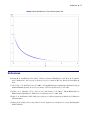
Consider the simple example of minimizing the Branin function,
f .x/ D
x2
5:1 2
5
x1 C x1
2
4
2
6
C 10 1
1
8
cos.x1 / C 10
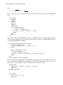
subject to 5 x1 10 and 0 x2 15 (Jones, Perttunen, and Stuckman 1993). The minimum function
value is f .x / D 0:397887 at x D . ; 12:275/; .; 2:275/; .9:42478; 2:475/: You can use the following
statements to solve this problem:
data vardata;
input _id_ $ _lb_ _ub_;
datalines;
x1 -5 10
x2 0 15
;
proc fcmp outlib=sasuser.myfuncs.mypkg;
function branin(x1, x2);
pi = constant('PI');
y1 = (x2-(5.1/(4*pi**2))*x1*x1+5*x1/pi-6)**2;
y2 = 10*(1-1/(8*pi))*cos(x1);
return (y1+y2+10);
endsub;
run;
data objdata;
input _id_ $ _function_ $ _sense_ $;
datalines;
f branin min
;
options cmplib
proc optlso
primalout =
variables =
objective =
performance
run;
= sasuser.myfuncs;
solution
vardata
objdata;
nthreads=4;
proc print data=solution;
run;
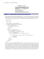
The OBJECTIVE= option in the PROC OPTLSO statement refers to the OBJDATA data set, which identifies
BRANIN as the name of the objective function that is defined in the FCMP library sasuser.myfuncs and
specifies that BRANIN should be minimized. The VARIABLES= option in the PROC OPTLSO statement
names the decision variables x1 and x2 and specifies lower and upper bounds. The PERFORMANCE
statement specifies the number of threads that PROC OPTLSO can use.
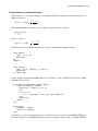
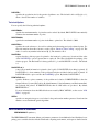
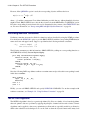
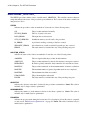
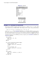
Figure 3.1 shows the ODS tables that the OPTLSO procedure produces by default.
Introductory Examples F 17
Figure 3.1 Bound-Constrained Problem: Output
The OPTLSO Procedure
Performance Information
Execution Mode
Single-Machine
Number of Threads 4
Problem Summary
Problem Type
NLP
Objective Definition Set
OBJDATA
Variables
VARDATA
Number of Variables
2
Integer Variables
0
Continuous Variables
2
Number of Constraints
0
Linear Constraints
0
Nonlinear Constraints
0
Objective Definition Source OBJDATA
Objective Sense
Minimize
Solution Summary
Solution Status
Function convergence
Objective
0.3978873689
Infeasibility
0
Iterations
32
Evaluations
1805
Cached Evaluations 36
Global Searches
1
Population Size
80
Seed
1
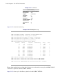
Obs _sol_ _id_ _value_
1
0 _obj_ 0.39789
2
0 _inf_ 0.00000
3
0 x1
9.42482
4
0 x2
2.47508
5
0 f
0.39789
Adding a Linear Constraint
You can use a LINCON= option to specify general linear equality or inequality constraints of the following
form:
n
X
j D1
aij xj f j D j g bi
for i D 1; : : : ; m
18 F Chapter 3: The OPTLSO Procedure
For example, suppose that in addition to the bound constraints on the decision variables, you need to guarantee
that the sum x1 C x2 is less than or equal to 0.6. To guarantee this, you can add a LINCON= option to the
previous data set definitions, as in the following statements:
data lindata;
input _id_ $ _lb_ x1 x2 _ub_;
datalines;
a1 . 1 1 0.6
;
proc optlso
variables = vardata
objective = objdata
lincon
= lindata;
run;
Here the symbol A1 denotes the name of the given linear constraints that are specified in the _ID_ column.
The corresponding lower and upper bounds are specified in the _LB_ and _UB_ columns, respectively.
Nonlinear Constraints on the Decision Variables
You can specify general nonlinear equality or inequality constraints by using the NLINCON= option and
adding its definition to the existing PROC FCMP library. Consider the previous problem with the following
additional constraint:
x12
2x2 14
You can specify this constraint by adding a new FCMP function library and providing it a corresponding
name and bounds in the NLINCON= option, as in the following statements:
data condata;
input _id_ $ _lb_ _ub_;
datalines;
c1 14 .
;
proc fcmp outlib=sasuser.myfuncs.mypkg;
function c1(x1, x2);
return (x1**2 - 2*x2);
endsub;
run;
proc optlso
variables
objective
lincon
nlincon
run;
=
=
=
=
vardata
objdata
lindata
condata;
By calling PROC FCMP a second time, you can append the definition of C1 to your existing user library.
That is, you do not need to redefine BRANIN after it has been added.
Introductory Examples F 19
A Simple Maximum Likelihood Example
The following is a very simple example of a maximum likelihood estimation problem that uses the loglikelihood function:
1 x 2
l.; / D log. /
2
The maximum likelihood estimates of the parameters and form the solution to
X
max
li .; /
;
i
where > 0 and
li .; / D
log. /
1 xi 2
2
The following sets of statements demonstrate two ways to formulate this example problem:
data lkhvar;
input _id_ $ _lb_;
datalines;
mu
.
sigma 0
;
data lkhobj1;
input _id_ $ _function_ $ _sense_ $;
datalines;
f loglkh1 max
;
In the following statements, the FCMP function is “stand-alone” because all the necessary data are defined
within the function itself:
proc fcmp outlib=sasuser.myfuncs.mypkg;
function loglkh1(mu, sigma);
array x[5] / nosym (1 3 4 5 7);
s=0;
do j=1 to 5;
s = s - log(sigma) - 0.5*((x[j]-mu)/sigma)**2;
end;
return (s);
endsub;
run;
proc optlso
variables = lkhvar
objective = lkhobj1;
run;
Alternatively, you can use an external data set to store the necessary observations and run PROC OPTLSO to
feed each observation to an FCMP function that processes a single line of data. In this case, PROC OPTLSO
20 F Chapter 3: The OPTLSO Procedure
sums the results for you. This mode is particularly useful when the data set is large and possibly distributed
over a set of nodes, as shown in “Example 3.7: Using External Data Sets” on page 59.
The following statements demonstrate how to store the necessary observations in an external data set for use
with PROC FCMP:
data logdata;
input x @@;
datalines;
1 3 4 5 7
;
data lkhobj2;
input _id_ $ _function_ $ _sense_ $ _dataset_ $;
datalines;
f loglkh2 max logdata
;
proc fcmp outlib=sasuser.myfuncs.mypkg;
function loglkh2(mu, sigma, x);
return (-log(sigma) -0.5*((x-mu)/sigma)**2);
endsub;
run;
proc optlso
variables = lkhvar
objective = lkhobj2;
run;
In this case, for each line of data in the data set logdata, the FCMP function LOGLKH2 is called. It is
important that the non-variable arguments of LOGLKH2 coincide with a subset of the column names in
logdata, in this case X. However, the order in which the variables and data column names appear is not
important. The following definition would work as well:
data lkhobj3;
input _id_ $ _function_ $ _sense_ $ _dataset_ $;
datalines;
f loglkh3 max logdata
;
proc fcmp outlib=sasuser.myfuncs.mypkg;
function loglkh3(x, sigma, mu);
return (- log(sigma) - 0.5*((x-mu)/sigma)**2);
endsub;
run;
proc optlso
variables = lkhvar
objective = lkhobj3;
run;
Syntax: OPTLSO Procedure F 21
Syntax: OPTLSO Procedure
The following statements are available in the OPTLSO procedure:
PROC OPTLSO <options> ;
READARRAY SAS-data-set-1 <SAS-data-set-2 : : : SAS-data-set-k> ;
PERFORMANCE <options> ;
PROC OPTLSO Statement
PROC OPTLSO <options> ;
The PROC OPTLSO statement invokes the OPTLSO procedure.
Functional Summary
Table 3.1 outlines the options available in the PROC OPTLSO statement.
Table 3.1 Summary of PROC OPTLSO Options
Description
Input Data Set Options
Specifies the input cache file
Specifies the initial genetic algorithm population
Describes the linear constraints
Indicates that the description uses the mathematical
programming system (MPS) data format
Describes the nonlinear constraints
Describes the objective function
Specifies the initial trial points
Indicates that the description uses the quadratic
programming system (QPS) data format
Describes the variables
Output Data Set Options
Specifies the output cache file
Specifies the local solutions and best feasible solution
Specifies the members of the genetic algorithm population
on exit
Stopping Condition Options
Specifies the absolute function convergence criterion
Specifies the maximum number of function evaluations
Specifies the maximum number of genetic algorithm
iterations
Specifies the upper limit on real time
option
CACHEIN=
FIRSTGEN=
LINCON=
MPSDATA=
NLINCON=
OBJECTIVE=
PRIMALIN=
QPSDATA=
VARIABLES=
CACHEOUT=
PRIMALOUT=
LASTGEN=
ABSFCONV=
MAXFUNC=
MAXGEN=
MAXTIME=
22 F Chapter 3: The OPTLSO Procedure
Description
Optimization Control Options
Specifies the feasibility tolerance
Specifies the number of global searches
Specifies the number of local searches
Genetic algorithm population size
Technical Options
Specifies the cache tolerance
Specifies the maximum cache size
Specifies the maximum size of the Pareto-optimal set
Specifies how frequently to print the solution progress
Specifies how much detail of solution progress to print in
the log
Enables or disables the printing summary
Initializes the seed for sampling routines
option
FEASTOL=
NGLOBAL=
NLOCAL=
POPSIZE=
CACHETOL=
CACHEMAX=
PARETOMAX=
LOGFREQ=
LOGLEVEL=
PRINTLEVEL=
SEED=
Input Data Set Options
You can specify the following options that are related to input data sets:
CACHEIN=SAS-data-set
names a previously computed sample set. Using a previously computed sample set enables PROC
OPTLSO to warm-start. It is crucial that the nonlinear objective and function values be identical to
those that were used when the cache data set was generated. For more information, see the section
“Specifying and Returning Trial Points” on page 38.
FIRSTGEN=SAS-data-set
specifies an initial sample set that defines a subset of the initial population. The columns of this data set
should coincide with the same format that is used by the PRIMALIN= data set. If the population size p
is smaller than the size of this set, only the first p points of this set are used. For more information, see
the section “Specifying and Returning Trial Points” on page 38.
LINCON=SAS-data-set
uses a dense format to describe the optimization problem’s linear constraints. The corresponding
data set should have columns _LB_ and _UB_ to describe lower and upper bounds, respectively.
The column _ID_ is reserved for the corresponding constraint name. The remaining columns must
correspond to the linear coefficients of the variables that are listed in the VARIABLES= option. For
more information, see the section “Describing Linear Constraints” on page 33.
MPSDATA=SAS-data-set
specifies a data set that can be used as a sparse alternative to the LINCON= option, which uses
a dense format to define variables. Mathematical programming system (MPS) is a common file
format for representing linear and mixed-integer mathematical programs. For an example of using the
OPTMODEL procedure to create the corresponding MPS file, see “Example 3.2: Using MPS Format”
on page 46. Internally, binary variables are converted into integer variables with lower and upper
bounds of 0 and 1, respectively. For more information, see the section “Describing Linear Constraints”
on page 33.
PROC OPTLSO Statement F 23
NLINCON=SAS-data-set
names the FCMP functions to be used from the current library as nonlinear constraints, along with
respective bounds. This data set should contain three columns: _ID_ to specify the corresponding
FCMP function names and _LB_ and _UB_ to specify the lower and upper bounds for the corresponding
constraints, respectively. For more information, see the section “Describing Nonlinear Constraints” on
page 34.
OBJECTIVE=SAS-data-set
names the FCMP functions to be used from the current library to form the objective. At a minimum,
this data set should have three columns: _ID_ to specify the function name to be used internally by the
solver, _FUNCTION_ to specify the corresponding FCMP function, and _SENSE_ to specify whether
the objective is to be minimized or maximized. PROC OPTLSO enables you to implicitly define your
objective function by using an external data set and an intermediate FCMP function definition that
can be used as placeholders to store temporary terms with respect to the external data set. For more
information, see the section “Describing the Objective Function” on page 28.
PRIMALIN=SAS-data-set
specifies an initial sample set to be evaluated. Initial data sets might be useful over a sequence of runs
when you want to ensure that PROC OPTLSO generates points that are at least as good as your current
best solution. This option is more general than the FIRSTGEN= option because points that are defined
in this data set might or might not be used to define the initial population for the genetic algorithm
(GA). For more information, see the section “Specifying and Returning Trial Points” on page 38.
QPSDATA=SAS-data-set
specifies a data set that can be used as a sparse alternative to the LINCON= option, which uses a
dense format to define variables. Quadratic programming system (QPS) is a common file format
for representing linear and mixed-integer mathematical programs that have quadratic terms in the
objective function. This option differs from the MPSDATA= option in that any quadratic terms in
the objective can be included in the data set. Do not use this option if the problem does not have
quadratic terms. For an example of using PROC OPTMODEL to create the corresponding QPS file,
see “Example 3.3: Using QPS Format” on page 49. Internally, binary variables are converted into
integer variables with lower and upper bounds of 0 and 1, respectively.
VARIABLES=SAS-data-set
stores the variable names, bounds, type, and scale. These names must match corresponding names,
FCMP functions, and related data sets. For more information, see the section “The Variable Data Set”
on page 27.
Output Data Set Options
You can specify the following options that are related to output data sets:
CACHEOUT=SAS-data-set
specifies the data set to which all completed function evaluations are output. For more information, see
the section “Specifying and Returning Trial Points” on page 38.
LASTGEN=SAS-data-set
specifies the data set to which the members of the current genetic algorithm population are returned
on exit. If more than one genetic algorithm is used, the data set combines the members from each
population into a single data set.
24 F Chapter 3: The OPTLSO Procedure
PRIMALOUT=SAS-data-set
specifies the output solution set. You can use this data set in future solves as the input set for the
PRIMALIN= option. For more information, see the section “Specifying and Returning Trial Points”
on page 38.
Stopping Condition Options
You can specify the following options that determine when to stop optimization:
ABSFCONV=r [n]
specifies an absolute function convergence criterion. PROC OPTLSO stops when the changes in the
objective function and constraint violation values in successive iterations meet the criterion
jf .x .k
1/
/
f .x .k/ /j C j.x .k
1/
/
.x .k/ /j r
where .x/ denotes the maximum constraint violation at point x. The optional integer value n specifies
the number of successive iterations for which the criterion must be satisfied before the process is
terminated. The default is r =1E–6 and n=10. To cause an early exit, you must specify a value for n
that is less than the value of the MAXGEN= option.
MAXFUNC=i
specifies the maximum number of function calls in the optimization process. The actual number of
function evaluations can exceed this number in order to ensure deterministic results.
MAXGEN=i
specifies the maximum number of genetic algorithm iterations. The default is 500.
MAXTIME=r
specifies an upper limit in seconds on the real time used in the optimization process. The actual running
time of PROC OPTLSO optimization might be longer because the actual running time includes the
remaining time needed to finish current function evaluations, the time for the output of the (temporary)
results, and (if required) the time for saving the results to appropriate data sets. By default, the
MAXTIME= option is not used.
Optimization Control Options
You can specify the following options to tailor the solver to your specific optimization problem:
FEASTOL=r
specifies a feasibility tolerance for provided constraints. Specify r 1E–9. The default is r =1E–3.
NGLOBAL=i
specifies the number of genetic algorithms to create, with each algorithm working on a separate
population of the size specified by the POPSIZE= option. Specify i as an integer greater than 0.
NLOCAL=i
specifies the number of local solvers to create. Specify i as an integer greater than 0. The default is
twice the number of variables in the problem.
PERFORMANCE Statement F 25
POPSIZE=i
specifies the population size for the genetic algorithm to use. The default is 40 ceil.log.n/ C 1/,
where n denotes the number of variables.
Technical Options
You can specify the following technical options:
CACHEMAX=i
specifies the maximum number of points that can be cached. By default, PROC OPTLSO automatically
calculates the maximum number of points.
PARETOMAX=i
specifies the maximum number of points in the Pareto-optimal set. The default is 5,000.
CACHETOL=r
specifies the cache tolerance to be used for caching and referencing previously evaluated points. For
more information about this tolerance, see the section “Function Value Caching” on page 39. The
value of r can be any number in the interval Œ0; 1. The default is 1E–9.
LOGFREQ=i
requests that the solution progress be printed to the iteration log after every i iterations if the value
of the LOGLEVEL= option is greater than or equal to 0. The value i =0 disables the printing of the
solution progress. The final iteration is always printed if i 1 and LOGLEVEL is nonzero. The default
is 1.
LOGLEVEL=0 | 1
controls how much information is printed to the log file. If LOGLEVEL=0, nothing is printed. If
LOGLEVEL=1, a short summary of the problem description and final solution status is printed. If
LOGLEVEL=0, this option overrides the LOGFREQ= option. By default, LOGLEVEL=1.
PRINTLEVEL=0 | 1
specifies whether to print a summary of the problem and solution. If PRINTLEVEL=1, then the
Output Delivery System (ODS) tables ProblemSummary, SolutionSummary, and PerformanceInfo
are produced and printed. If PRINTLEVEL=0, then no ODS tables are produced. By default,
PRINTLEVEL=1.
For more information about the ODS tables that are created by PROC OPTLSO, see the section “ODS
Tables” on page 41.
SEED=i
specifies a nonnegative integer as a seed value for the pseudorandom number generator. Pseudorandom
numbers are used within the genetic algorithm.
PERFORMANCE Statement
PERFORMANCE <options> ;
The PERFORMANCE statement defines performance parameters for multithreaded and distributed computing, passes variables that describe the distributed computing environment, and requests detailed results
26 F Chapter 3: The OPTLSO Procedure
about the performance characteristics of a SAS high-performance analytics procedure. For more information
about the options available for the PERFORMANCE statement, see Chapter 4, “Shared Concepts and Topics”
(SAS/OR User’s Guide: Mathematical Programming), and Chapter 3, “Shared Concepts and Topics” (Base
SAS Procedures Guide: High-Performance Procedures).
Note that the SAS High-Performance Optimization license is required to invoke PROC OPTLSO in distributed
mode. For examples of running in distributed mode see the third program in “Example 3.7: Using External
Data Sets” on page 59 and “Example 3.8: Johnson’s Systems of Distributions” on page 65.
READARRAY Statement
READARRAY SAS-data-set-1 <SAS-data-set-2 : : : SAS-data-set-k> ;
PROC FCMP (see “The FCMP Procedure” on page 27) provides the READ_ARRAY function to read data
from a SAS data set into array variables. In order to ensure that the referenced data sets are available, PROC
OPTLSO also requires that the names of these data sets be provided as a list of names in the READARRAY
statement. For an example, see the second program in “Example 3.7: Using External Data Sets” on page 59.
The following example creates and reads a SAS data set into an FCMP array variable:
data barddata;
input y @@;
datalines;
0.14 0.18 0.22 0.25 0.29
0.32 0.35 0.39 0.37 0.58
0.73 0.96 1.34 2.10 4.39
;
proc fcmp outlib=sasuser.myfuncs.mypkg;
function bard(x1, x2, x3);
array y[15] / nosym;
rc = read_array('barddata', y);
fx = 0;
do k=1 to 15;
dk = (16-k)*x2 + min(k,16-k)*x3;
fxk = y[k] - (x1 + k/dk);
fx = fx + fxk**2;
end;
return (0.5*fx);
endsub;
run;
options cmplib = sasuser.myfuncs;
data _null_;
bval = bard(1,2,3);
put bval=;
run;
Here the call to READ_ARRAY in the PROC FCMP function definition of Bard populates the array Y with
the rows of the BardData data set. If the Bard function were subsequently used in a problem definition for
PROC OPTLSO, the BardData data set should be listed in the corresponding READARRAY statement of
PROC OPTLSO as demonstrated in the second program in “Example 3.7: Using External Data Sets” on
page 59.
Details: OPTLSO Procedure F 27
Details: OPTLSO Procedure
The OPTLSO procedure uses a hybrid combination of genetic algorithms (Goldberg 1989; Holland 1975),
which optimize integer and continuous variables, and generating set search (Kolda, Lewis, and Torczon
2003), which performs local search on the continuous variables to improve the robustness of both algorithms.
Both genetic algorithms (GAs) and the generating set search (GSS) have proven to be effective algorithms
for many classes of derivative-free optimization problems. When only continuous variables are present, a
GA usually requires more function evaluations than a GSS to converge to a minimum. This is partly due
to the GA’s need to simultaneously perform a global search of the solution space. In a hybrid setting, the
requirement for the GA to find accurate local minima can be relaxed, and internal parameters can be tuned
toward finding promising starting points for the GSS.
The FCMP Procedure
The FCMP procedure is part of Base SAS software and is the primary mechanism in SAS for creating
user-defined functions to be used in a DATA step and many SAS procedures. You can use most of the SAS
programming statements and SAS functions that you can use in a DATA step to define FCMP functions
and subroutines. The OPTLSO procedure also uses PROC FCMP to provide a general gateway for you to
describe objective and constraint functions. For more information, see the sections “Describing the Objective
Function” on page 28 and “Describing Nonlinear Constraints” on page 34), respectively.
However, there are a few differences between the capabilities of the DATA step and the FCMP procedure.
For more information, see the documentation about the FCMP procedure in Base SAS Procedures Guide.
Further, not all PROC FCMP functionality is currently compatible with PROC OPTLSO; in particular, the
following FCMP functions are not supported and should not be called within your FCMP function definitions:
WRITE_ARRAY, RUN_MACRO, and RUN_SASFILE. The READ_ARRAY function is supported; however,
the corresponding data sets that are used must be listed in a separate statement of PROC OPTLSO (see the
section “READARRAY Statement” on page 26 and the second program in “Example 3.7: Using External
Data Sets” on page 59). After you define your objective and constraint functions, you must specify the
libraries by using the CMPLIB= system option in the OPTIONS statement. For more information about the
OPTIONS statement, see SAS Statements: Reference. For more information about the CMPLIB= system
option, see SAS System Options: Reference.
The Variable Data Set
The variable data set can have up to five columns. The variable names are described in the _ID_ column.
These names are used to map variable values to identically named FCMP function variable arguments. Lower
and upper bounds on the variables are defined in columns _LB_ and _UB_, respectively. You can manually
enter scaling for each variable by using the _SCALE_ column. Derivative-free optimization performance can
often be greatly improved by scaling the variables appropriately. By default, the scale vector is defined in a
manner similar to that described in Griffin, Kolda, and Lewis (2008). If integer variables are present, the
_TYPE_ column value signifies that a given variable is either C for continuous or I for integer. By default, all
variables are assumed to be continuous.
28 F Chapter 3: The OPTLSO Procedure
You can use the VARIABLES= option to specify the SAS data set that describes the variables to be optimized.
For example, suppose you want to specify the following set of variables, where x1 and x2 are continuous and
x3 is an integer variable:
0 x1 1000
0 x2 0:001
0 x3 4
You can specify this set of variables by using the following DATA step:
data vardata;
input _id_ $ _lb_ _ub_ _type_ $;
datalines;
x1 0 1000 C
x2 0 0.001 C
x3 0 4
I
;
By default, variables are automatically scaled. PROC OPTLSO uses this scaling along with the cache
tolerance when PROC OPTLSO builds the function value cache. For more information about scaling, see the
section “Function Value Caching” on page 39. You can provide your own scaling by setting a _SCALE_
column in the variable data set as follows:
data vardata;
input _id_ $ _lb_ _ub_ _type_ $ _scale_;
datalines;
x1 0 1000 C 1000
x2 0 0.001 C 0.5
x3 0 4
I 2
;
When derivative-free optimization is performed, proper scaling of variables can dramatically improve
performance. Default scaling takes into account the lower and upper bounds, so you are encouraged to
provide the best estimates possible.
Describing the Objective Function
PROC OPTLSO enables you to define the function explicitly by using PROC FCMP. The following statements
describe a PROC FCMP objective function that is used in “Example 3.5: Linear Constraints and a Nonlinear
Objective” on page 54:
proc fcmp outlib=sasuser.myfuncs.mypkg;
function sixhump(x1,x2);
return ((4 - 2.1*x1**2 + x1**4/3)*x1**2
+ x1*x2 + (-4 + 4*x2**2)*x2**2);
endsub;
run;
Because PROC FCMP writes to an external library that might contain a large number of functions, PROC
OPTLSO needs to know which objective function in the FCMP library to use and whether to minimize
or maximize the function. You provide this information to PROC OPTLSO by specifying an objective
Describing the Objective Function F 29
description data set in the OBJECTIVE= option. To minimize the function sixhump, you could specify the
OBJECTIVE= objdata option and define the following objective description data set:
data objdata;
input _id_ $ _function_ $ _sense_ $;
datalines;
f
sixhump
min
;
In the preceding DATA step, the _ID_ column specifies the function name to be used internally by the solver,
the _FUNCTION_ column specifies the corresponding FCMP function name, and the _SENSE_ column
specifies whether the objective is to be minimized or maximized.
Intermediate Functions
You can use intermediate functions to simplify the objective function definition and to improve computational
efficiency. You specify intermediate functions by using a missing value entry in the _SENSE_ column to
denote that the new function is not an objective. The _ID_ column entries for intermediate functions can then
be used as arguments for the objective function. The following set of programming statements demonstrates
how to create an equivalent objective definition for “Example 3.5: Linear Constraints and a Nonlinear
Objective” on page 54 by using intermediate functions.
data objdata;
length _function_ $10;
input _id_ $ _function_ $ _sense_ $;
datalines;
f1
sixhump1
.
f2
sixhump2
.
f3
sixhumpNew
min
;
proc fcmp outlib=sasuser.myfuncs.mypkg;
function sixhump1(x1,x2);
return (4 - 2.1*x1**2 + x1**4/3);
endsub;
function sixhump2(x1,x2);
return (-4 + 4*x2**2);
endsub;
function sixhumpNew(x1,x2,f1,f2);
return (f1*x1**2 + x1*x2 + f2*x2**2);
endsub;
run;
In this case, PROC OPTLSO first computes the values for sixhump1 and sixhump2, internally assigning the
output to f1 and f2, respectively. The _ID_ column entries for intermediate functions can then be used as
arguments for the objective function f3. Because the intermediate functions are evaluated first, before the
objective function is evaluated, intermediate functions should never depend on output from the objective
function.
Incorporating MPS and QPS Objective Functions
If you use the MPSDATA= or QPSDATA= options to define linear constraints, an objective function m.x/ is
necessarily defined (see “Describing Linear Constraints” on page 33). If you do not specify the OBJECTIVE=
option, PROC OPTLSO optimizes m.x/. However, if you specify the OBJECTIVE= option, the objective
30 F Chapter 3: The OPTLSO Procedure
function m.x/ is ignored unless you explicitly include the corresponding objective function name and specify
whether the function is to be used as an intermediate or objective function. (See “Example 3.4: Combining
MPS and FCMP Function Definitions” on page 51.) If the objective name also matches a name in the FCMP
library, the FCMP function definition takes precedence.
Using Large Data Sets
When your objective function includes the sum of a family of functions that are parameterized by the rows
of a given data set, PROC OPTLSO enables you to include in your objective function definition a single
external data set that is specified in the _DATASET_ column of the OBJECTIVE= data set. Consider the
following unconstrained optimization problem, where k is a very large integer (for example, 106 ), A denotes
a k 5 matrix, and b denotes the corresponding right-hand-side target vector:
min f .x/ D kAx
bk2 C kxk1
x2R5
To evaluate the objective function, the following operations must be performed:
f1 .x/ D
f2 .x/ D
k
X
i D1
5
X
di
jxi j
j D1
f .x/ D
p
f1 .x/ C f2 .x/
where
0
di D @ bi C
5
X
12
aij xj A
j D1
and aij denotes the jth entry of row i of the matrix A. Assume that there is an existing SAS data set that
stores numerical entries for A and b. The following DATA step shows an example data set, where k D 3:
data Abdata;
input _id_ $ a1 a2 a3 a4 a5 b;
datalines;
row1 1 2 3 4 5 6
row2 7 8 9 10 11 12
row3 13 14 15 16 17 18
;
The following statements pass this information to PROC OPTLSO by adding the corresponding functions to
the FCMP function library Sasuser.Myfuncs.Mypkg:
proc fcmp outlib=sasuser.myfuncs.mypkg;
function axbi(x1,x2,x3,x4,x5,a1,a2,a3,a4,a5,b);
array x[5];
array a[5];
di = -b;
do j=1 to 5;
Describing the Objective Function F 31
di = di + a[j]*x[j];
end;
return (di*di);
endsub;
function onenorm(x1,x2,x3,x4,x5);
array x[5];
f2 = 0;
do j=1 to 5;
f2 = f2 + abs(x[j]);
end;
return (f2);
endsub;
function combine(f1, f2);
return (sqrt(f1)+f2);
endsub;
run;
The next DATA step then defines the objective name with a given target:
data lsqobj1;
input _id_ $ _function_$ _sense_ $ _dataset_ $;
datalines;
f1
axbi
.
Abdata
f2
onenorm
.
.
f
combine
min
.
;
The following DATA step declares the variables:
data xvar;
input _id_ $ @@;
datalines;
x1 x2 x3 x4 x5
;
The following statements call the OPTLSO procedure:
options cmplib=sasuser.myfuncs;
proc optlso
variables = xvar
objective = lsqobj1;
run;
The contents of the OBJECTIVE= data set (lsqobj1) direct PROC OPTLSO to search for the three FCMP
functions AXBI, ONENORM, and COMBINE in the library that is specified by the CMPLIB= option. The
missing values in the _SENSE_ column indicate that AXBI and ONENORM are intermediate functions to be
used as arguments of the objective function COMBINE, which is of type MIN. Of the three FCMP functions,
only F1 has requested data. The entry Abdata specifies that the FCMP function AXBI should be called on
each row of the data set Abdata and that the results should be summed. This value is then specified as the
first argument to the FCMP function COMBINE.
In this example, Abdata is a data set that comes from the Work library. However, Abdata could just as
easily come from a data set in a user-defined library or even a data set that had been previously distributed
32 F Chapter 3: The OPTLSO Procedure
(for example, to a Teradata or Greenplum database). If the data set Abdata is stored in a different library,
replace Abdata with libref.Abdata in the data set lsqob1. The source of the data set is irrelevant to PROC
OPTLSO.
You can omit F2 if you want to form the one-norm directly in the aggregate function. Thus, an equivalent
formulation would be as follows:
proc fcmp outlib=sasuser.myfuncs.mypkg;
function combine2(x1,x2,x3,x4,x5, f1);
array x[5];
f2 = 0;
do j=1 to 5;
f2 = f2 + abs(x[j]);
end;
return (sqrt(f1)+f2);
endsub;
run;
In this case, you define the objective name with a given target in a data set:
data lsqobj2;
input _id_ $ _function_$ _sense_ $ _dataset_ $;
datalines;
f1
axbi
.
Abdata
f
combine2
min
.
;
options cmplib=sasuser.myfuncs;
proc optlso
variables = xvar
objective = lsqobj2;
run;
Thus, any of the intermediate functions that are used within the OBJECTIVE= data set (objdata) are permitted
to have arguments that form a subset of the variables listed in the VARIABLES= data set (xvar) and the
numerical columns from the data set that is specified in the _DATASET_ column of the OBJECTIVE= data
set. Only numerical values are supported from external data sets. Only one function can be of type MIN or
MAX. This function can take as arguments any of the variables in the VARIABLES= data set, any of the
numerical columns from an external data set for the objective (if specified), and any implicit variables that
are listed in the _ID_ column of the OBJECTIVE= data set.
The following rules for the objective data set are used during parsing:
• Only one data set can be used for a given problem definition.
• The objective function can take a data set as input only if no intermediate functions are being used.
Otherwise, only the intermediate functions can be linked to the corresponding data set.
The data set is used in a distributed format if either the NODES= option is specified in the PERFORMANCE
statement or the data set is a distributed library.
Describing Linear Constraints F 33
Describing Linear Constraints
The preferred method for describing linear constraints is to use the LINCON=, MPSDATA=, or QPSDATA=
option. You should not describe linear constraints by using the NLINCON= option because they are treated
as black-box constraints and can degrade performance.
If you have only a few variables and linear constraints, you might prefer to use the dense format to describe
your linear constraints by specifying both the LINCON= option and the VARIABLES= option. Suppose a
problem has the following linear constraints:
1
1
2x1 4x3
15
3x1 C 7x2 13
x1 C x2 C x3 D 11
The following DATA step formulates this information as an input data set for PROC OPTLSO:
data lcondata;
input _id_ $
datalines;
a1 -1
2 0 -4
a2 1
-3 7 0
a3 11
1 1 1
;
_lb_ x1-x3 _ub_;
15
13
11
Linear constraints are handled by using tangent search directions that are defined with respect to nearby
constraints. The metric that is used to determine when a constraint is sufficiently near might cause the
algorithm to temporarily treat range constraints as equality constraints. For this reason, it is preferable
that you not separate a range constraint into two inequality constraints. For example, although both of the
following range constraint formulations are equivalent, the former is preferred:
1 2x1
4x3 15
2x1
1 2x1
4x3 15
4x3
and
Even for a moderate number of variables and constraints, using the dense format to describe the linear
constraints can be burdensome. As an alternative, you can construct a sparse formulation by using MPSformat (or QPS-format) SAS data sets and specifying the MPSDATA= (or QPSDATA=) option in PROC
OPTLSO. For more information about these data sets, see Chapter 17, “The MPS-Format SAS Data Set”
(SAS/OR User’s Guide: Mathematical Programming). You can easily create these data sets by using
the OPTMODEL procedure, as demonstrated in “Example 3.2: Using MPS Format” on page 46 and
“Example 3.3: Using QPS Format” on page 49. For more information about using PROC OPTMODEL to
create MPS data sets, see Chapter 5, “The OPTMODEL Procedure” (SAS/OR User’s Guide: Mathematical
Programming).
Both MPS and QPS data sets require that you define an objective function. Although the QPS standard
supports a constant term, the MPS standard does not; thus any constant term that is defined in PROC
OPTMODEL is naturally dropped and not included in the corresponding data set. In particular, if the
MPSDATA= option is used, the corresponding objective will have the form
m.x/ D c T x
34 F Chapter 3: The OPTLSO Procedure
However, if the QPSDATA= option is used, the corresponding objective will have the form
1
m.x/ D c T x C x T Qx C K
2
where c, Q, and the constant term K are defined within the provided data sets. Although multiple objectives
might be listed, PROC OPTLSO uses only the first objective from the MPSDATA= or QPSDATA= option.
How the corresponding objective function is used is determined by the contents of the OBJECTIVE= data
set. For more information, see “Incorporating MPS and QPS Objective Functions” on page 29.
Describing Nonlinear Constraints
Nonlinear constraints are treated as black-box functions and are described by using the FCMP procedure.
You should use the NLINCON= option to provide PROC OPTLSO with the corresponding FCMP function
names and lower and upper bounds. Suppose a problem has the following nonlinear constraints:
1
x1 x2 x3 C sin.x2 /
1
x1 x2 C x1 x3 C x2 x3 D 1
The following statements pass this information to PROC OPTLSO by adding two corresponding functions to
the FCMP function library Sasuser.Myfuncs.Mypkg:
proc fcmp outlib=sasuser.myfuncs.mypkg;
function con1(x1, x2, x3);
return (x1*x2*x3 + sin(x2));
endsub;
function con2(x1, x2, x3);
return (x1*x2 + x1*x3 + x3*x3);
endsub;
run;
Next, the following DATA step defines nonlinear constraint names and provides their corresponding bounds
in the data set condata:
data condata;
input _id_ $ _lb_ _ub_;
datalines;
con1 -1 1
con2 1 1
;
Finally, you can call PROC OPTLSO and specify NLINCON=CONDATA. For another example with
nonlinear constraints, see “Example 3.6: Using Nonlinear Constraints” on page 56.
The OPTLSO Algorithm
The OPTLSO algorithm is based on a genetic algorithm (GA). GAs are a family of local search algorithms
that seek optimal solutions to problems by applying the principles of natural selection and evolution. Genetic
algorithms can be applied to almost any optimization problem and are especially useful for problems for
which other calculus-based techniques do not work, such as when the objective function has many local
The OPTLSO Algorithm F 35
optima, when the objective function is not differentiable or continuous, or when solution elements are
constrained to be integers or sequences. In most cases, genetic algorithms require more computation than
specialized techniques that take advantage of specific problem structures or characteristics. However, for
optimization problems for which no such techniques are available, genetic algorithms provide a robust general
method of solution.
In general, genetic algorithms use some variation of the following process to search for an optimal solution:
initialization:
An initial population of solutions is randomly generated, and the
objective function is evaluated for each member of this initial
iteration.
selection:
Individual members of the current iteration are chosen stochastically either to parent the next iteration or to be passed on to it
such that the members that are the fittest are more likely to be
selected. A solution’s fitness is based on its objective value, with
better objective values reflecting greater fitness.
crossover:
Some of the selected solutions are passed to a crossover operator. The crossover operator combines two or more parents
to produce new offspring solutions for the next iteration. The
crossover operator tends to produce new offspring that retain the
common characteristics of the parent solutions while combining
the other traits in new ways. In this way, new areas of the search
space are explored while attempting to retain optimal solution
characteristics.
mutation:
Some of the next-iteration solutions are passed to a mutation
operator, which introduces random variations in the solutions.
The purpose of the mutation operator is to ensure that the solution
space is adequately searched to prevent premature convergence
to a local optimum.
repeat:
The current iteration of solutions is replaced by the new iteration.
If the stopping criterion is not satisfied, the process returns to the
selection phase.
The crossover and mutation operators are commonly called genetic operators. Selection and crossover
distinguish genetic algorithms from a purely random search and direct the algorithm toward finding an
optimum.
There are many ways to implement the general strategy just outlined, and it is also possible to combine the
genetic algorithm approach with other heuristic solution improvement techniques. In the traditional genetic
algorithm, the solution space is composed of bit strings, which are mapped to an objective function, and
the genetic operators are modeled after biological processes. Although there is a theoretical foundation for
the convergence of genetic algorithms that are formulated in this way, in practice most problems do not
fit naturally into this paradigm. Modern research has shown that optimizations can be set up by using the
natural solution domain (for example, a real vector or integer sequence) and by applying crossover and
mutation operators that are analogous to the traditional genetic operators but are more appropriate to the
natural formulation of the problem.
Although genetic algorithms have been demonstrated to work well for a variety of problems, there is
no guarantee of convergence to a global optimum. Also, the convergence of genetic algorithms can be
36 F Chapter 3: The OPTLSO Procedure
sensitive to the choice of genetic operators, mutation probability, and selection criteria, so that some initial
experimentation and fine-tuning of these parameters are often required.
The OPTLSO procedure seeks to automate this process by using hybrid optimization in which several genetic
algorithms can run in parallel and each algorithm is initialized with different default option settings. PROC
OPTLSO also adds a step to the GA; this step permits generating set search (GSS) algorithms to be used on a
selected subset of the current population. GSS algorithms are designed for problems that have continuous
variables and have the advantage that, in practice, they often require significantly fewer evaluations than GAs
to converge. Furthermore, GSS can provide a measure of local optimality that is very useful in performing
multimodal optimization.
The following additional “growth steps” are used whenever continuous variables are present:
local search selection:
A small subset of points are selected based
on their fitness score and distance to (1) other
points and (2) pre-existing locally optimal
points.
local search optimization:
Local search optimization begins concurrently
for each selected point. The only modification
made to the original optimization problem is
that the variables’ lower and upper bounds are
modified to temporarily fix integer variables to
their current setting.
These additional growth steps are performed for each iteration; they permit selected members of the population
(based on diversity and fitness) to benefit from local optimization over the continuous variables. If only
integer variables are present, this step is not used.
Multiobjective Optimization
Many practical optimization problems involve more than one objective criterion, so the decision maker needs
to examine trade-offs between conflicting objectives. For example, for a particular financial model you might
want to maximize profit while minimizing risk, or for a structural model you might want to minimize weight
while maximizing strength. The desired result for such problems is usually not a single solution, but rather
a range of solutions that can be used to select an acceptable compromise. Ideally each point represents a
necessary compromise in the sense that no single objective can be improved without worsening at least one
remaining objective. The goal of PROC OPTLSO in the multiobjective case is thus to return to the decision
maker a set of points that represent the continuum of best-case scenarios. Multiobjective optimization is
performed in PROC OPTLSO whenever more than one objective function of type MIN or MAX exists. For
an example, see “Example 3.10: Multiobjective Optimization” on page 72.
Mathematically, multiobjective optimization can be defined in terms of dominance and Pareto optimality.
For a k-objective minimizing optimization problem, a point x is dominated by a point y if fi .x/ fi .y/ for
all i = 1,. . . ,k and fj .x/ > fj .y/ for some j = 1,. . . ,k.
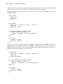
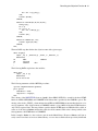
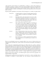
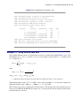
A Pareto-optimal set contains only nondominated solutions. In Figure 3.2, a Pareto-optimal frontier is plotted
with respect to minimization objectives f1 .x/ and f2 .x/ along with a corresponding population of 10 points
that are plotted in the objective space. In this example, point a dominates fe; f; kg, b dominates fe; f; g; kg, c
Multiobjective Optimization F 37
dominates fg; h; kg, and d dominates fk; ig. Although c is not dominated by any other point in the population,
it has not yet converged to the true Pareto-optimal frontier. Thus there exist points in a neighborhood of c
that have smaller values of f1 and f2 .
Figure 3.2 Pareto-Optimal Set
f2 .x/
k
f
e
a
g
b
h
c
i
d
f1 .x/
In the constrained case, a point x is dominated by a point y if .x/ > and .y/ < .x/, where .x/ denotes
the maximum constraint violation at point x and FEASTOL=I thus feasibility takes precedence over objective
function values.
Genetic algorithms enable you to attack multiobjective problems directly in order to evolve a set of Paretooptimal solutions in one run of the optimization process instead of solving multiple separate problems. In
addition, local searches in neighborhoods around nondominated points can be conducted to improve objective
function values and reduce crowding. Because the number of nondominated points that are encountered
might be greater than the total population size, PROC OPTLSO stores nondominated points in an archived
set N ; you can specify the PARETOMAX= option to control the size of this set.
Although it is difficult to verify directly that a point lies on the true Pareto-optimal frontier without using
derivatives, convergence can indirectly be measured by monitoring movement of the population with respect to
N , the current set of nondominated points. A number of metrics for measuring convergence in multiobjective
evolutionary algorithms have been suggested, such as the generational distance by Van Veldhuizen (1999),
the inverted generational distance by Coello Coello and Cruz Cortes (2005), and the averaged Hausdorff
distance by Schütze et al. (2012). PROC OPTLSO uses a variation of the averaged Hausdorff distance that is
extended for general constraints.
Distance between sets is computed in terms of the distance between a point and a set, which in turn is defined
in terms of the distance between two points. The distance measure used by PROC OPTLSO for two points x
and y is calculated as
d.x; y/ D j.x/
.y/j C
k
X
jfi .x/
fi .y/j
i D1
where .x/ denotes the maximum constraint violation at point x. Then the distance between a point x and a
set A is defined as
d.x; A/ D min d.x; y/
y2A
38 F Chapter 3: The OPTLSO Procedure
Let Fj denote the set of all nondominated points within the current population at the start of generation j. Let
Nj denote the set of all nondominated points at the start of generation j. At the beginning of each generation,
Fj Nj is always satisfied. Then progress made during iteration j+1 is defined as
Progress.j C 1/ D
1 X
d.x; Nj C1 /
jFj j
x2Fj
Because d.x; Nj C1 / D 0 whenever x 2 Fj \ Fj C1 , the preceding sum is over the set of points in the
population that move from a status of nondominated to dominated. In this case, the progress made is measured
as the distance to the nearest dominating point.
Specifying and Returning Trial Points
You can use the following options to initialize PROC OPTLSO with user-specified points: CACHEIN=,
FIRSTGEN=, and PRIMALIN=. You can use the following options to have trial points returned to you:
CACHEOUT=, LASTGEN=, and PRIMALOUT=.
Both input and output point data sets have the following columns:
_SOL_
specifies the point’s unique solution tag.
_ID_
specifies the variable and (function) ID name.
_VALUE_
specifies the variable (function) value.
Input Data Sets
The following DATA step generates 30 random points for the initial population if the variables x 2 R5 have
bounds 5 xi 10:
data popin;
low = -5.0;
upp = 10.0;
numpoints = 30;
dim = 5;
do _sol_=1 to numpoints;
do i=1 to dim;
_id_= compress("x" || put(i, 4.0));
_value_ = low + (upp-low)*ranuni(2);
output;
end;
end;
keep _sol_ _id_ _value_;
run;
You can then use this data set as input for the OPTLSO procedure by using the FIRSTGEN= option.
Function Value Caching F 39
Output Data Sets
PROC OPTLSO dynamically creates and reports on two metadata functions for you: the true objective (which
is a combination of the FCMP objective and the linear and quadratic terms) and the maximum constraint
violation. These functions are assigned the following function ID names (therefore, these names should not
be used as variable, constraint, or function names):
_OBJ_
specifies the point’s objective. N OTE : This value is omitted when solving a multiobjective problem.
_INF_
specifies the point’s maximum constraint violation.
Output data sets have additional rows that correspond to the problem’s FCMP functions. These rows must
exist for the data set specified in the CACHEIN= option, but they should be omitted for the data sets specified
in the FIRSTGEN= and PRIMALIN= options.
When you observe the solution output, it might be easier to compare points if they are listed as rows rather
than as columns. SAS provides a variety of ways to transform the results for your purposes. For example, if
you prefer that the rows of the data sets correspond to individual points, you can use the following statements
to transpose the returned data set, where popout denotes the data set that is returned by PROC OPTLSO:
proc transpose data=popout out=poprow (drop=_label_ _name_);
by _sol_;
var _value_;
id _id_;
run;
Function Value Caching
To improve performance, the OPTLSO procedure implements a caching system. This caching system helps
reduce the overall workload of the solver by eliminating duplicate function evaluations. As the individual
optimizers (citizens) submit new trial points for evaluation, the points are saved in the cache along with
their function evaluation values. Then, before beginning the potentially expensive function evaluations for
a new trial point, PROC OPTLSO determines whether a similar point already exists within the cache. If a
similar point is found in the cache, its function values are immediately returned for the newly submitted point.
Returning function values from the cache instead of duplicating the effort of computing new function values
can lead to significant performance improvements for the overall procedure.
The cache is implemented as a splay tree, similar to that used in Gray and Kolda (2006); Hough, Kolda,
and Patrick (2000). The splay tree rebalances itself as new points are added to the cache. This rebalancing
ensures that recently added or accessed points are maintained at the root of the tree and are therefore available
for quick retrieval. This splay tree data structure lends itself nicely to the needs of a caching system.
When determining whether a newly submitted trial point has a similar point already in the cache, PROC
OPTLSO compares the new trial point to all previous trial points by using the value of the CACHETOL=
option in the PROC OPTLSO statement. This value specifies a tolerance to use in comparing two points and
determining whether the two points are similar enough. In addition to the CACHETOL= value, the cache
comparison also takes into account the _SCALE_ values that are specified as part of the variable data set that
is specified in the VARIABLES= option.
40 F Chapter 3: The OPTLSO Procedure
Two points x and y are considered cache equivalent if
jxi
yi j si ; for i D 1; : : : ; n
where s denotes the corresponding scaling vector. Thus, if a point x has been evaluated (or is being evaluated)
and a point y is submitted for evaluation and satisfies the preceding criteria, y is “cache evaluated” instead of
being evaluated directly. In this case, y is associated with f .x/ and c.x/. Although the splay tree is very
efficient, the cache lookup time for quick evaluation might eventually dominate the evaluation process time.
You can use the CACHEMAX= option to limit the size of the cache.
Even when the FCMP functions are not defined, the cache system helps to avoid redundant computations
when the linear constraints are explicitly handled.
Iteration Log
The iteration log provides detailed information about the progress of the OPTLSO procedure. The log appears
by default or if LOGLEVEL=1. The iteration log provides the following information:
Iteration
Displays the number of completed genetic algorithm iterations.
Best Objective
Displays the best objective found at each iteration with respect to the current
setting of the FEASTOL= option. N OTE : This column is included only for
single-objective optimization.
Nondom
Displays the number of nondominated solutions in the current Pareto-optimal set.
N OTE : This column is included only for multiobjective optimization.
Progress
Displays a numerical indication of the progress being made from one iteration
to the next. For a description of how this value is computed, see the section
“Multiobjective Optimization” on page 36. N OTE : This column is included only
for multiobjective optimization.
Infeasibility
Displays the aggregate constraint violation of the current best point.
Evals
Displays the cumulative number of function evaluations.
Time
Displays the time needed to achieve current best solution.
Procedure Termination Messages
After PROC OPTLSO terminates, one of the following messages is displayed:
User interrupted.
The procedure was interrupted by the user.
Function convergence criteria reached.
The best objective value and feasibility have not sufficiently improved for the specified number of
iterations. This criterion is a typical exit state if the global optimum is reached early in the algorithm.
ODS Tables F 41
Maximum function evaluations reached.
PROC OPTLSO has attempted to exceed the maximum number of function evaluations.
Generations complete.
The maximum number of GA generations (iterations) has been reached. At this point, no new points
are generated, and the algorithm exits.
Maximum time reached.
PROC OPTLSO has exceeded the maximum allotted time.
Problem may be unbounded.
The objective value appears to take on arbitrarily large values at points that satisfy the feasibility
tolerance.
Infeasible.
The problem is infeasible.
Failed.
The algorithm exited for any reason other than the preceding reasons. For example, this message is
displayed if the provided FCMP function does not exist or cannot be evaluated.
ODS Tables
PROC OPTLSO creates three Output Delivery System (ODS) tables by default. The first table, ProblemSummary, is a summary of the input problem. The second table, SolutionSummary, is a brief summary of the
solution status. The third table, PerformanceInfo, is a summary of performance options. You can use ODS
table names to select tables and create output data sets. For more information about ODS, see SAS Output
Delivery System: Procedures Guide.
If you specify the DETAILS option in the PERFORMANCE statement, then the Timing table is also produced.
Table 3.4 lists all the ODS tables that can be produced by the OPTLSO procedure, along with the statement
and option specifications that are required to produce each table.
Table 3.4 ODS Tables Produced by PROC OPTLSO
ODS Table Name
ProblemSummary
SolutionSummary
PerformanceInfo
Timing
Description
Summary of the input optimization
problem
Summary of the solution status
Statement
PROC OPTLSO
List of performance options and
their values
Detailed solution timing
PROC OPTLSO
PROC OPTLSO
PERFORMANCE
Option
PRINTLEVEL=1
(default)
PRINTLEVEL=1
(default)
PRINTLEVEL=1
(default)
DETAILS
42 F Chapter 3: The OPTLSO Procedure
Macro Variable _OROPTLSO_
The OPTLSO procedure defines a macro variable named _OROPTLSO_. This variable contains a character
string that indicates the status of the procedure upon termination. The contents of the macro variable are
interpreted as follows.
STATUS
indicates the procedure’s status at termination. It can take one of the following values:
OK
The procedure terminated normally.
SYNTAX_ERROR
The use of syntax is incorrect.
DATA_ERROR
The input data are inconsistent.
OUT_OF_MEMORY
Insufficient memory was allocated to the procedure.
IO_ERROR
A problem in reading or writing of data has occurred.
SEMANTIC_ERROR
An evaluation error, such as an invalid operand type, has occurred.
ERROR
The status cannot be classified into any of the preceding categories.
SOLUTION_STATUS
indicates the status of the solution at termination. It can take one of the following values:
ABORTED
The user signaled that the procedure should terminate.
ABSFCONV
The procedure terminated on the absolute function convergence criterion.
INFEASIBLE
Problem is globally infeasible. Only returned if all constraints are linear.
MAXFUNC
The procedure terminated on the maximum number of function evaluations.
MAXGEN
The maximum number of genetic algorithm iterations was completed.
MAXTIME
The maximum time limit was reached.
UNBOUNDED
The problem might be unbounded.
FAILED
The status cannot be classified into any of the preceding categories.
OBJECTIVE
indicates the objective value that is obtained by the procedure at termination. N OTE : This value is
included only for single-objective optimization.
NONDOMINATED
indicates the number of nondominated solutions in the Pareto-optimal set. N OTE : This value is
included only for multiobjective optimization.
PROGRESS
indicates the progress made during the last iteration. For a description of how this value is computed,
see the section “Multiobjective Optimization” on page 36. N OTE : This value is included only for
multiobjective optimization.
Examples: OPTLSO Procedure F 43
INFEASIBILITY
indicates the level of infeasibility of the constraints at the solution.
EVALUATIONS
indicates the total number of evaluations that were not cached.
ITERATIONS
indicates the number of iterations that were required to solve the problem.
SETUP_TIME
indicates the real time (in seconds) that is taken to set up the optimization problem and distribute data.
SOLUTION_COUNT
indicates number of solutions that are returned in the PRIMALIN= data set if that option was specified.
SOLUTION_TIME
indicates the real time (in seconds) that is taken by the procedure to perform iterations for solving the
problem.
Examples: OPTLSO Procedure
Example 3.1: Using Dense Format
This example uses data from Floudas and Pardalos (1992) and illustrates how to use the VARIABLES= and
LINCON= options in conjunction with the OBJECTIVE= option. The problem has nine linear constraints
and a quadratic objective function. Suppose you want to minimize
f .x/ D 5
4
X
xi
i D1
5
4
X
i D1
xi2
13
X
xi
iD5
subject to
2x1 C 2x2 C x10 C x11 10
2x1 C 2x3 C x10 C x12 10
2x1 C 2x3 C x11 C x12 10
8x1 C x10 0
8x2 C x11 0
8x3 C x12 0
2x4 x5 C x10 0
2x6 x7 C x11 0
2x8 x9 C x12 0
and
0 xi 1;
0 xi 100;
0 x13 1
i D 1; 2; : : : ; 9
i D 10; 11; 12
44 F Chapter 3: The OPTLSO Procedure
The following statements use the dense format to define the linear constraints:
data vardata;
input _id_ $ _lb_ _ub_;
datalines;
x1 0
1
x2 0
1
x3 0
1
x4 0
1
x5 0
1
x6 0
1
x7 0
1
x8 0
1
x9 0
1
x10 0 100
x11 0 100
x12 0 100
x13 0
1
;
proc fcmp outlib=sasuser.myfuncs.mypkg;
function quadobj(x1,x2,x3,x4,x5,x6,x7,x8,x9,x10,x11,x12,x13);
sum1 = 5*(x1 + x2 + x3 + x4);
sum2 = 5*(x1**2 + x2**2 + x3**2 + x4**2);
sum3 = (x5 + x6 + x7 + x8 + x9 + x10 + x11 + x12 + x13);
return (sum1 - sum2 - sum3);
endsub;
run;
data objdata;
input _id_ $ _function_ $ _sense_ $;
datalines;
f
quadobj
min
;
data lindata;
input _id_ $ _lb_ x1-x13 _ub_;
datalines;
a1 . 2 2 0 0 0 0 0 0 0 1
a2 . 2 0 2 0 0 0 0 0 0 1
a3 . 2 0 2 0 0 0 0 0 0 0
a4 . -8 0 0 0 0 0 0 0 0 1
a5 . 0 -8 0 0 0 0 0 0 0 0
a6 . 0 0 -8 0 0 0 0 0 0 0
a7 . 0 0 0 -2 -1 0 0 0 0 1
a8 . 0 0 0 0 0 -2 -1 0 0 0
a9 . 0 0 0 0 0 0 0 -2 -1 0
;
options cmplib
proc optlso
primalout =
objective =
variables =
= sasuser.myfuncs;
solution
objdata
vardata
1
0
1
0
1
0
0
1
0
0
1
1
0
0
1
0
0
1
0 10
0 10
0 10
0 0
0 0
0 0
0 0
0 0
0 0
Example 3.1: Using Dense Format F 45
lincon
= lindata;
performance nthreads=2;
run;
proc print data=solution;
run;
The VARIABLES=VARDATA option in the PROC OPTLSO statement specifies the variables and their
respective bounds. The objective function is defined by using PROC FCMP and the objective function
name QUADOBJ. Other properties are described in the SAS data set objdata. The linear constraints are
specified by using the SAS data set lindata, in which each row stores the (zero and nonzero) coefficients of
the corresponding linear constraint along with their respective lower and upper bounds. The problem
description is then passed to the OPTLSO procedure by using the options VARIABLES=VARDATA,
OBJECTIVE=OBJDATA, and LINCON=LINDATA. The PERFORMANCE statement specifies the number
of threads that PROC OPTLSO can use.
Output 3.1.1 shows the output from running these statements.
Output 3.1.1 Using Dense Format
The OPTLSO Procedure
Performance Information
Execution Mode
Single-Machine
Number of Threads 2
Problem Summary
Problem Type
NLP
Linear Constraints
LINDATA
Objective Definition Set
OBJDATA
Variables
VARDATA
Number of Variables
13
Integer Variables
0
Continuous Variables
13
Number of Constraints
9
Linear Constraints
9
Nonlinear Constraints
0
Objective Definition Source OBJDATA
Objective Sense
Minimize
46 F Chapter 3: The OPTLSO Procedure
Output 3.1.1 continued
Solution Summary
Solution Status
Function convergence
Objective
-15.00099275
Infeasibility
0.0009927519
Iterations
32
Evaluations
3956
Cached Evaluations 356
Global Searches
1
Population Size
160
Seed
1
Obs _sol_ _id_
_value_
1
0 _obj_ -15.0010
2
0 _inf_
0.0010
3
0 x1
1.0000
4
0 x2
1.0000
5
0 x3
1.0000
6
0 x4
1.0000
7
0 x5
1.0000
8
0 x6
1.0000
9
0 x7
1.0000
10
0 x8
1.0000
11
0 x9
1.0000
12
0 x10
3.0000
13
0 x11
3.0000
14
0 x12
3.0010
15
0 x13
1.0000
16
0 f
-15.0010
Example 3.2: Using MPS Format
In this example, the linear component of the same problem definition as in Example 3.1 is described by using
the OPTMODEL procedure and is saved as an MPS data set. The quadratic objective is then defined by using
the FCMP function QUADOBJ.
Because PROC OPTMODEL outputs an MPS data set that uses array notation, you can use the following
macro definition to strip brackets from the resulting data set:
%macro lsompsmod(setold,setnew);
data &setnew(drop=i);
set &setold;
array FC{*} _CHARACTER_;
do i=1 to dim(FC);
FC[i] = compress(FC[i], "[]");
end;
run;
%mend;
Example 3.2: Using MPS Format F 47
For more complicated array structures, take care to ensure that the resulting transformation is well defined.
Next, you run a PROC OPTMODEL step that outputs a MPS data set, followed by the newly defined
%LSOMPSMOD macro to strip brackets, followed by a PROC OPTLSO step that takes as input the MPS
data set that was output by PROC OPTMODEL and transformed by the %LSOMPSMOD macro.
proc optmodel;
var x{1..13} >= 0 <= 1;
for {i in 10..12} x[i].ub = 100;
min z = 0;
con a1: 2*x[1] + 2*x[2] + x[10] +
con a2: 2*x[1] + 2*x[3] + x[10] +
con a3: 2*x[1] + 2*x[3] + x[11] +
con a4: -8*x[1] + x[10] <= 0;
con a5: -8*x[2] + x[11] <= 0;
con a6: -8*x[3] + x[12] <= 0;
con a7: -2*x[4] - x[5] + x[10] <=
con a8: -2*x[6] - x[7] + x[11] <=
con a9: -2*x[8] - x[9] + x[12] <=
save mps lindataOld;
quit;
x[11] <= 10;
x[12] <= 10;
x[12] <= 10;
0;
0;
0;
%lsompsmod(lindataOld, lindata);
proc optlso
primalout =
mpsdata
=
objective =
performance
run;
solution
lindata
objdata;
nthreads=2;
proc print data=solution;
run;
Output 3.2.1 shows the output from running these steps.
Output 3.2.1 Using MPS Format
The OPTLSO Procedure
Performance Information
Execution Mode
Single-Machine
Number of Threads 2
48 F Chapter 3: The OPTLSO Procedure
Output 3.2.1 continued
Problem Summary
Problem Type
NLP
MPS Data Set
LINDATA
Objective Definition Set
OBJDATA
Number of Variables
13
Integer Variables
0
Continuous Variables
13
Number of Constraints
9
Linear Constraints
9
Nonlinear Constraints
0
Objective Definition Source OBJDATA
Objective Sense
Minimize
Solution Summary
Solution Status
Function convergence
Objective
-15.00099275
Infeasibility
0.0009927519
Iterations
32
Evaluations
3956
Cached Evaluations 356
Global Searches
1
Population Size
160
Seed
1
Obs _sol_ _id_
_value_
1
0 _obj_ -15.0010
2
0 _inf_
0.0010
3
0 x1
1.0000
4
0 x2
1.0000
5
0 x3
1.0000
6
0 x4
1.0000
7
0 x5
1.0000
8
0 x6
1.0000
9
0 x7
1.0000
10
0 x8
1.0000
11
0 x9
1.0000
12
0 x10
3.0000
13
0 x11
3.0000
14
0 x12
3.0010
15
0 x13
16
0 f
-15.0010
17
0 z
0.0000
1.0000
Example 3.3: Using QPS Format F 49
Example 3.3: Using QPS Format
In this example, the entire problem definition is first described in the following PROC OPTMODEL step and
is then saved as a QPS data set in the subsequent PROC OPTLSO step. In this case, no FCMP function needs
to be defined.
proc optmodel;
var x{1..13} >= 0 <= 1;
for {i in 10..12} x[i].ub = 100;
min z = 5*sum{i in 1..4} x[i]
- 5*sum{i in 1..4} x[i]**2 - sum{i in 5..13} x[i];
con a1: 2*x[1] + 2*x[2] + x[10] + x[11] <= 10;
con a2: 2*x[1] + 2*x[3] + x[10] + x[12] <= 10;
con a3: 2*x[1] + 2*x[3] + x[11] + x[12] <= 10;
con a4: -8*x[1] + x[10] <= 0;
con a5: -8*x[2] + x[11] <= 0;
con a6: -8*x[3] + x[12] <= 0;
con a7: -2*x[4] - x[5] + x[10] <= 0;
con a8: -2*x[6] - x[7] + x[11] <= 0;
con a9: -2*x[8] - x[9] + x[12] <= 0;
save qps qpdata;
quit;
proc optlso
primalout = solution
qpsdata
= qpdata;
performance nthreads=2;
run;
proc print data=solution;
run;
Note that in this case the objective definition is taken directly from the QPS data set qpdata. Output 3.3.1
shows the output from running these steps.
50 F Chapter 3: The OPTLSO Procedure
Output 3.3.1 Using QPS Format
The OPTLSO Procedure
Performance Information
Execution Mode
Single-Machine
Number of Threads 2
Problem Summary
Problem Type
QP
QPS Data Set
QPDATA
Number of Variables
13
Integer Variables
0
Continuous Variables
13
Number of Constraints
9
Linear Constraints
9
Nonlinear Constraints
0
Objective Definition Source QPDATA
Objective Sense
Minimize
Solution Summary
Solution Status
Function convergence
Objective
-15.00099275
Infeasibility
0.0009927519
Iterations
32
Evaluations
3956
Cached Evaluations 356
Global Searches
1
Population Size
160
Seed
1
Example 3.4: Combining MPS and FCMP Function Definitions F 51
Output 3.3.1 continued
Obs _sol_ _id_
_value_
1
0 _obj_ -15.0010
2
0 _inf_
0.0010
3
0 x[1]
1.0000
4
0 x[2]
1.0000
5
0 x[3]
1.0000
6
0 x[4]
1.0000
7
0 x[5]
1.0000
8
0 x[6]
1.0000
9
0 x[7]
1.0000
10
0 x[8]
1.0000
11
0 x[9]
1.0000
12
0 x[10]
3.0000
13
0 x[11]
3.0000
14
0 x[12]
3.0010
15
0 x[13]
16
0 z
1.0000
-15.0010
Example 3.4: Combining MPS and FCMP Function Definitions
In this example, the linear component of the same problem definition as in Example 3.1 is described by using
the OPTMODEL procedure and is saved as an MPS data set. The quadratic component of the objective is
then defined by using the FCMP function QUADOBJ.
As in “Example 3.2: Using MPS Format” on page 46, you can use the macro definition lsompsmod to strip
brackets from the resulting data set:
%macro lsompsmod(setold,setnew);
data &setnew(drop=i);
set &setold;
array FC{*} _CHARACTER_;
do i=1 to dim(FC);
FC[i] = compress(FC[i], "[]");
end;
run;
%mend;
For more complicated array structures, take care to ensure that the resulting transformation is well defined.
Next you run a PROC OPTMODEL step that outputs a MPS data set, followed by the %LSOMPSMOD
macro, followed by the PROC FCMP step that defines the FCMP function QUADOBJ, followed by a
PROC OPTLSO step that takes as input both the MPS data set that was output by PROC OPTMODEL and
transformed by the %LSOMPSMOD macro and the quadratic component of the objective that was defined
by PROC FCMP.
52 F Chapter 3: The OPTLSO Procedure
proc optmodel;
var x{1..13} >= 0 <= 1;
for {i in 10..12} x[i].ub = 100;
min linobj = 5*sum{i in 1..4} x[i] - sum{i
con a1: 2*x[1] + 2*x[2] + x[10] + x[11] <=
con a2: 2*x[1] + 2*x[3] + x[10] + x[12] <=
con a3: 2*x[1] + 2*x[3] + x[11] + x[12] <=
con a4: -8*x[1] + x[10] <= 0;
con a5: -8*x[2] + x[11] <= 0;
con a6: -8*x[3] + x[12] <= 0;
con a7: -2*x[4] - x[5] + x[10] <= 0;
con a8: -2*x[6] - x[7] + x[11] <= 0;
con a9: -2*x[8] - x[9] + x[12] <= 0;
save mps lindataOld;
quit;
%lsompsmod(lindataOld, lindata);
in 5..13} x[i];
10;
10;
10;
proc fcmp outlib=sasuser.myfuncs.mypkg;
function quadobj(x1,x2,x3,x4,f1);
return (f1 - 5*(x1**2 + x2**2 + x3**2 + x4**2));
endsub;
run;
data objdata;
input _id_ $ _function_ $ _sense_ $;
datalines;
f1 linobj
.
f
quadobj
min
;
options cmplib
proc optlso
primalout =
mpsdata
=
objective =
performance
run;
= sasuser.myfuncs;
solution
lindata
objdata;
nthreads=2;
proc print data=solution;
run;
Output 3.4.1 shows the output from running these steps.
Output 3.4.1 Using MPS Format
The OPTLSO Procedure
Performance Information
Execution Mode
Single-Machine
Number of Threads 2
Example 3.4: Combining MPS and FCMP Function Definitions F 53
Output 3.4.1 continued
Problem Summary
Problem Type
NLP
MPS Data Set
LINDATA
Objective Definition Set
OBJDATA
Number of Variables
13
Integer Variables
0
Continuous Variables
13
Number of Constraints
9
Linear Constraints
9
Nonlinear Constraints
0
Objective Definition Source
OBJDATA
Objective Sense
Minimize
Objective Intermediate Functions 1
Solution Summary
Solution Status
Function convergence
Objective
-15.00099275
Infeasibility
0.0009927519
Iterations
32
Evaluations
3956
Cached Evaluations 356
Global Searches
1
Population Size
160
Seed
1
Obs _sol_ _id_
_value_
1
0 _obj_ -15.0010
2
0 _inf_
0.0010
3
0 x1
1.0000
4
0 x2
1.0000
5
0 x3
1.0000
6
0 x4
1.0000
7
0 x5
1.0000
8
0 x6
1.0000
9
0 x7
1.0000
10
0 x8
1.0000
11
0 x9
1.0000
12
0 x10
3.0000
13
0 x11
3.0000
14
0 x12
3.0010
15
0 x13
1.0000
16
0 f
17
0 f1
4.9990
18
0 linobj
4.9990
-15.0010
54 F Chapter 3: The OPTLSO Procedure
Example 3.5: Linear Constraints and a Nonlinear Objective
The problem in this example is to minimize the six-hump camel-back function (Michalewicz 1996, Appendix
B). Minimize
!
x14
2
f .x/ D 4 2:1x1 C
x12 C x1 x2 C 4 C 4x22 x22
3
subject to
2x1 C x2 x1 x2 x1 C 2x2 2
2
2
Providing derivative-free algorithms with good estimates for lower and upper bounds often greatly improves
performance because it prevents the algorithm from unnecessarily sampling in regions that you do not want
to explore. For this problem, the following statements add the explicit variable bounds 2 x1 2 and
2 x2 2:
data xbnds;
input _id_ $ _lb_ _ub_;
datalines;
x1 -2 2
x2 -2 2
;
data lindata;
input _id_ $ _lb_ x1 x2 _ub_;
datalines;
a1
. 2 1 2
a2 -2 1 -1 .
a3 -2 1 2 .
;
data objdata;
input _id_ $ _function_ $ _sense_ $;
datalines;
f
sixhump
min
;
proc fcmp outlib=sasuser.myfuncs.mypkg;
function sixhump(x1,x2);
return ((4 - 2.1*x1**2 + x1**4/3)*x1**2 + x1*x2 + (-4 + 4*x2**2)*x2**2);
endsub;
run;
options cmplib
proc optlso
primalout =
variables =
objective =
lincon
=
= sasuser.myfuncs;
solution
xbnds
objdata
lindata;
Example 3.5: Linear Constraints and a Nonlinear Objective F 55
performance nthreads=2;
run;
proc print data=solution;
run;
Output 3.5.1 shows the output from running these steps.
Output 3.5.1 Linear Constraints and a Nonlinear Objective
The OPTLSO Procedure
Performance Information
Execution Mode
Single-Machine
Number of Threads 2
Problem Summary
Problem Type
NLP
Linear Constraints
LINDATA
Objective Definition Set
OBJDATA
Variables
XBNDS
Number of Variables
2
Integer Variables
0
Continuous Variables
2
Number of Constraints
3
Linear Constraints
3
Nonlinear Constraints
0
Objective Definition Source OBJDATA
Objective Sense
Minimize
Solution Summary
Solution Status
Function convergence
Objective
-1.031628453
Infeasibility
0
Iterations
26
Evaluations
1474
Cached Evaluations 17
Global Searches
1
Population Size
80
Seed
1
Obs _sol_ _id_
_value_
1
0 _obj_ -1.03163
2
0 _inf_
3
0 x1
4
0 x2
5
0 f
0.00000
-0.08983
0.71265
-1.03163
56 F Chapter 3: The OPTLSO Procedure
Example 3.6: Using Nonlinear Constraints
The following optimization problem is discussed in Haverly (1978) and Liebman et al. (1986). This example
illustrates how to use PROC FCMP to define nonlinear constraints and use an MPS data set to define linear
constraints. Maximize
f .x/ D 9x1 C 15x2
6x3
16x4
10x5
subject to
x3 C x4 D x6 C x7
x6 C x8 D x1
x7 C x9 D x2
x8 C x9 D x5
2:5x1 x10 x6 2x8 0
1:5x2 x10 x7 2x9 0
3x3 C x4 x10 .x3 C x4 / D 0
and
0 x1 100
0 x2 200
1 x10 3
0 xi ; for i D 3; : : : ; 9
In the following steps, the linear component of the problem definition is first described in PROC OPTMODEL
and then saved as an MPS data set. Because the objective is linear, no FCMP objective function needs to be
used. In the second section of steps, the nonlinear constraints are defined by using FCMP functions, and
their corresponding names and lower and upper bounds are stored in the data set condata. The OPTLSO
procedure is then called with the options NLINCON=CONDATA and MPSDATA=NLCEX.
As in “Example 3.2: Using MPS Format” on page 46, you can use the macro definition lsompsmod to strip
brackets from the resulting data set:
%macro lsompsmod(setold,setnew);
data &setnew(drop=i);
set &setold;
array FC{*} _CHARACTER_;
do i=1 to dim(FC);
FC[i] = compress(FC[i], "[]");
end;
run;
%mend;
proc optmodel;
var x{1..10} >= 0;
x[10].lb = 1;
x[10].ub = 3;
x[1].ub = 100;
x[2].ub = 200;
con x[3] + x[4] = x[6] + x[7],
x[6] + x[8] = x[1],
Example 3.6: Using Nonlinear Constraints F 57
x[7] + x[9] = x[2],
x[8] + x[9] = x[5];
max f = 9*x[1] + 15*x[2] - 6*x[3] - 16*x[4] - 10*x[5];
save mps nlcexOld;
quit;
%lsompsmod(nlcexOld, nlcex);
proc fcmp outlib=sasuser.myfuncs.mypkg;
function nlc1(x1,x6,x8,x10);
return (2.5*x1 - x10*x6 - 2*x8);
endsub;
function nlc2(x2,x7,x9,x10);
return (1.5*x2 - x10*x7 - 2*x9);
endsub;
function nlc3(x3,x4,x10);
return (3*x3 + x4 - x10*(x3 + x4));
endsub;
run;
data condata;
input _id_ $ _lb_ _ub_;
datalines;
nlc1 0 .
nlc2 0 .
nlc3 0 0
;
options cmplib
proc optlso
primalout =
mpsdata
=
nlincon
=
logfreq
=
performance
run;
= sasuser.myfuncs;
solution
nlcex
condata
10;
nthreads=2;
proc print data=solution;
run;
Output 3.6.1 shows the ODS tables that are produced from running these steps.
Output 3.6.1 Using Nonlinear Constraints: ODS Tables
The OPTLSO Procedure
Performance Information
Execution Mode
Single-Machine
Number of Threads 2
58 F Chapter 3: The OPTLSO Procedure
Output 3.6.1 continued
Problem Summary
Problem Type
NLP
MPS Data Set
NLCEX
Nonlinear Constraints
CONDATA
Number of Variables
10
Integer Variables
0
Continuous Variables
10
Number of Constraints
7
Linear Constraints
4
Nonlinear Constraints
3
Objective Definition Source NLCEX
Objective Sense
Maximize
Solution Summary
Solution Status
Function convergence
Objective
400.0059833
Infeasibility
0.0009972793
Iterations
34
Evaluations
4054
Cached Evaluations 435
Global Searches
1
Population Size
160
Seed
1
Obs _sol_ _id_ _value_
1
0 _obj_ 400.006
2
0 _inf_
0.001
3
0 x1
0.000
4
0 x2
200.000
5
0 x3
0.000
6
0 x4
99.999
7
0 x5
100.001
8
0 x6
0.000
99.999
9
0 x7
10
0 x8
0.000
11
0 x9
100.001
12
0 x10
13
0 f
14
0 nlc1
0.000
15
0 nlc2
-0.001
16
0 nlc3
0.000
1.000
400.006
Output 3.6.2 shows the iteration log from running these steps.
Example 3.7: Using External Data Sets F 59
Output 3.6.2 Using Nonlinear Constraints: Log
NOTE: The OPTLSO procedure is executing in single-machine mode.
NOTE: The OPTLSO algorithm is using up to 2 threads.
NOTE: The problem has 10 variables (0 integer, 10 continuous).
NOTE: The problem has 7 constraints (4 linear, 3 nonlinear).
NOTE: The problem has 3 FCMP function definitions.
NOTE: The deterministic parallel mode is enabled.
Best
Iteration
Objective
Infeasibility
Evals
Time
1
0
11
399.9157119539
0
170
0
0
1299
21 400.004880426434
0
0.0008133715544
2448
0
31 400.005983302901 0.00099727927424
3685
0
34 400.005983302901 0.00099727927424
4054
0
NOTE: Function convergence criteria reached.
NOTE: There were 3 observations read from the data set WORK.CONDATA.
NOTE: The data set WORK.SOLUTION has 16 observations and 3 variables.
Example 3.7: Using External Data Sets
This example illustrates the use of external data sets that are specified in the OBJECTIVE= option. The
Bard function (Moré, Garbow, and Hillstrom 1981) is a least squares problem that has n D 3 parameters and
m D 15 functions fk ;
15
1X 2
f .x/ D
fk .x/;
2
x D .x1 ; x2 ; x3 /
kD1
where
fk .x/ D yk
with vk D 16
x1 C
k
vk x2 C wk x3
k, wk D min.uk ; vk /, and
y D .0:14; 0:18; 0:22; 0:25; 0:29; 0:32; 0:35; 0:39; 0:37; 0:58; 0:73; 0:96; 1:34; 2:10; 4:39/
The minimum function value f .x / = 4.107E–3 occurs at the point .0:08; 1:13; 2:34/. In this example, the
additional variable bounds 1000 xi 1000 for i D 1; 2; 3 are added.
There are three approaches to specifying the objective function. The first approach assumes that the necessary
data are stored within the FCMP function. In this case, you can specify the objective function without using
an external data set, as follows:
60 F Chapter 3: The OPTLSO Procedure
data vardata;
input _id_ $ _lb_ _ub_ ;
datalines;
x1 -1000 1000
x2 -1000 1000
x3 -1000 1000
;
data objdata;
input _id_ $ _function_ $ _sense_ $;
datalines;
f
bard
min
;
proc fcmp outlib=sasuser.myfuncs.mypkg;
function bard(x1, x2, x3);
array y[15] /nosym (0.14 0.18 0.22 0.25 0.29
0.32 0.35 0.39 0.37 0.58
0.73 0.96 1.34 2.10 4.39);
fx = 0;
do k=1 to 15;
vk = 16 - k;
wk = min(k,vk);
fxk = y[k] - (x1 + k/(vk*x2 + wk*x3));
fx = fx + fxk**2;
end;
return (0.5*fx);
endsub;
run;
options cmplib
proc optlso
primalout =
variables =
objective =
performance
run;
= sasuser.myfuncs;
solution
vardata
objdata;
nthreads=2;
proc print data=solution;
run;
Output 3.7.1 shows the output from running these steps.
Output 3.7.1 Using External Data Sets
The OPTLSO Procedure
Performance Information
Execution Mode
Single-Machine
Number of Threads 2
Example 3.7: Using External Data Sets F 61
Output 3.7.1 continued
Problem Summary
Problem Type
NLP
Objective Definition Set
OBJDATA
Variables
VARDATA
Number of Variables
3
Integer Variables
0
Continuous Variables
3
Number of Constraints
0
Linear Constraints
0
Nonlinear Constraints
0
Objective Definition Source OBJDATA
Objective Sense
Minimize
Solution Summary
Solution Status
Function convergence
Objective
0.0041074417
Infeasibility
0
Iterations
73
Evaluations
6261
Cached Evaluations 91
Global Searches
1
Population Size
120
Seed
1
Obs _sol_ _id_ _value_
1
0 _obj_ 0.00411
2
0 _inf_ 0.00000
3
0 x1
0.08239
4
0 x2
1.13238
5
0 x3
2.34437
6
0 f
0.00411
This approach is cumbersome if the size of the required data increases. A second approach for mediumsized data sets is to use the READ_ARRAY statement within the FCMP function definition. Because the
environment might be distributed, PROC OPTLSO requires a list of all data sets that are used in FCMP
function definitions to ensure that the corresponding data sets are available. This list should be specified by
using the READARRAY statement.
62 F Chapter 3: The OPTLSO Procedure
data barddata;
input y @@;
datalines;
0.14 0.18 0.22 0.25 0.29
0.32 0.35 0.39 0.37 0.58
0.73 0.96 1.34 2.10 4.39
;
data vardata;
input _id_ $ _lb_ _ub_ ;
datalines;
x1 -1000 1000
x2 -1000 1000
x3 -1000 1000
;
data objdata;
input _id_ $ _function_ $ _sense_ $;
datalines;
f
bard
min
;
proc fcmp outlib=sasuser.myfuncs.mypkg;
function bard(x1, x2, x3);
array y[15] /nosym;
rc = read_array('barddata', y);
fx = 0;
do k=1 to 15;
dk = (16-k)*x2 + min(k,16-k)*x3;
fxk = y[k] - (x1 + k/dk);
fx = fx + fxk**2;
end;
return (0.5*fx);
endsub;
run;
options cmplib = sasuser.myfuncs;
proc optlso
primalout = solution
variables = vardata
objective = objdata;
readarray barddata;
run;
proc print data=solution;
run;
Output 3.7.2 shows the output from running these statements.
Example 3.7: Using External Data Sets F 63
Output 3.7.2 Using External Data Sets (II)
The OPTLSO Procedure
Performance Information
Execution Mode
Single-Machine
Number of Threads 4
Data Access Information
Data
Engine Role Path
WORK.BARDDATA V9
Input On Client
Problem Summary
Problem Type
NLP
Objective Definition Set
OBJDATA
Variables
VARDATA
Number of Variables
3
Integer Variables
0
Continuous Variables
3
Number of Constraints
0
Linear Constraints
0
Nonlinear Constraints
0
Objective Definition Source OBJDATA
Objective Sense
Minimize
Solution Summary
Solution Status
Function convergence
Objective
0.0041074417
Infeasibility
0
Iterations
73
Evaluations
6261
Cached Evaluations 91
Global Searches
1
Population Size
120
Seed
1
Obs _sol_ _id_ _value_
1
0 _obj_ 0.00411
2
0 _inf_ 0.00000
3
0 x1
0.08239
4
0 x2
1.13238
5
0 x3
2.34437
6
0 f
0.00411
64 F Chapter 3: The OPTLSO Procedure
The preceding approach can be prohibitive if the size of the data set is large. As a third approach to specifying
the objective function, PROC OPTLSO provides an alternate data input gateway that is described in the
OBJECTIVE= data set, as shown in the following statements:
data vardata;
input _id_ $ _lb_ _ub_ ;
datalines;
x1 -1000 1000
x2 -1000 1000
x3 -1000 1000
;
data barddata;
k = _n_;
input y @@;
datalines;
0.14 0.18 0.22 0.25 0.29
0.32 0.35 0.39 0.37 0.58
0.73 0.96 1.34 2.10 4.39
;
data objdata;
input _id_ $ _function_ $ _sense_ $ _dataset_ $;
datalines;
fx
bard
min barddata
;
proc fcmp outlib=sasuser.myfuncs.mypkg;
function bard(x1, x2, x3, k, y);
vk = 16 - k;
wk = min(k,vk);
fxk = y - (x1 + k/(vk*x2 + wk*x3));
return (0.5*fxk**2);
endsub;
run;
options cmplib
proc optlso
primalout =
variables =
objective =
performance
run;
= sasuser.myfuncs;
solution
vardata
objdata;
nodes=2 nthreads=8;
proc print data=solution;
run;
Output 3.7.3 shows the output from running these statements.
Example 3.8: Johnson’s Systems of Distributions F 65
Output 3.7.3 Using External Data Sets (III)
The OPTLSO Procedure
Problem Summary
Problem Type
NLP
Objective Definition Set
OBJDATA
Variables
VARDATA
Number of Variables
3
Integer Variables
0
Continuous Variables
3
Number of Constraints
0
Linear Constraints
0
Nonlinear Constraints
0
Objective Definition Source OBJDATA
Objective Sense
Minimize
Objective Data Set
barddata
Solution Summary
Solution Status
Function convergence
Objective
0.0041074398
Infeasibility
0
Iterations
77
Evaluations
6438
Cached Evaluations 263
Global Searches
1
Population Size
120
Seed
1
Performance Information
Host Node
<< your grid host >>
Execution Mode
Distributed
Number of Compute Nodes
2
Number of Threads per Node 8
Example 3.8: Johnson’s Systems of Distributions
This example further illustrates the use of external data sets that are specified in the OBJECTIVE= option.
For this example, a data set that contains n D 20; 000 randomly generated observations is used to estimate
the parameters for the Johnson SU family of distributions (Bowman and Shenton 1983). The objective is the
log likelihood for the family, which involves four variables, x D .x1 ; x2 ; x3 ; x4 /:
f .x/ D n log.x4 /
n log.x2 /
n
1 X
.x3 C x4 log.zk //2 C log.1 C yk2 /
2
kD1
66 F Chapter 3: The OPTLSO Procedure
where
zk D yk C
q
1 C yk2 with yk D
dk
x1
x2
Here, dk denotes the value of d in the kth observation of the data set that is generated by the following DATA
step.
data sudata;
n=20000;
theta=-1;
sigma=1;
delta=3;
gamma=5;
rngSeed=123;
do i = 1 to n;
z = rannor(rngSeed);
a = exp( (z - gamma)/delta );
d = sigma * ( (a**2 - 1)/(2*a) ) + theta;
output;
end;
keep d;
run;
This generates a data set called sudata that contains n D 20; 000 observations. You can modify n to increase
or decrease the computational work per function evaluation. The following call to PROC FCMP defines the
corresponding FCMP function definition:
proc fcmp outlib=sasuser.myfuncs.mypkg;
function jsu(x4,x2,f1);
return (20000*(log(x4) - log(x2)) + f1);
endsub;
function jsu1(x1,x2,x3,x4,d);
yk = (d - x1)/x2;
zk = yk + sqrt(1 + yk**2);
return (-0.5*(x3 + x4*log(zk))**2 -0.5*log(1 + yk**2));
endsub;
run;
options cmplib = sasuser.myfuncs;
In the following steps, the assumption for the definition of jsu and jsu1 is that jsu1 is called once for each
line of data (in this case 20,000 times) and cumulatively summed. The resulting value is then provided to the
function jsu for a final calculation, which is called only once per evaluation of f .x/.
data objdata;
input _id_ $ _function_ $ _sense_ $ _dataset_ $;
datalines;
f1 jsu1 .
sudata
f jsu max .
;
data vardata;
input _id_ $ _lb_ _ub_;
datalines;
Example 3.8: Johnson’s Systems of Distributions F 67
x1
x2
x3
x4
;
.
1e-12
.
1e-12
.
.
.
.
proc optlso
primalout =
objective =
variables =
logfreq
=
maxgen
=
performance
run;
solution
objdata
vardata
100
1000;
nodes=4 nthreads=8;
Output 3.8.1 shows the output from running these steps.
Output 3.8.1 Estimation for Johnson SU Family of Distributions
The OPTLSO Procedure
Problem Summary
Problem Type
NLP
Objective Definition Set
OBJDATA
Variables
VARDATA
Number of Variables
4
Integer Variables
0
Continuous Variables
4
Number of Constraints
0
Linear Constraints
0
Nonlinear Constraints
0
Objective Definition Source
OBJDATA
Objective Sense
Maximize
Objective Intermediate Functions 1
Objective Data Set
sudata
Solution Summary
Solution Status
Function convergence
Objective
-8414.725097
Infeasibility
0
Iterations
879
Evaluations
75737
Cached Evaluations 1260
Global Searches
1
Population Size
120
Seed
1
68 F Chapter 3: The OPTLSO Procedure
Output 3.8.1 continued
Performance Information
Host Node
<< your grid host >>
Execution Mode
Distributed
Number of Compute Nodes
4
Number of Threads per Node 8
Example 3.9: Discontinuous Function with a Lookup Table
This example illustrates the ability of PROC OPTLSO to optimize a discontinuous function. The example
generates a data set of discrete values that approximate a given smooth nonlinear function. The function
being optimized is simply using that data set as a lookup table to find the appropriate discretized value.
%let N = 100;
%let L = 0;
%let U = 10;
options cmplib = sasuser.myfuncs;
proc fcmp outlib=sasuser.myfuncs.mypkg;
function SmoothFunc(x);
y = x*sin(x) + x*x*cos(x);
return (y);
endsub;
function DiscretizedFunc(x);
array lookup[&N, 2] / nosymbols;
rc = read_array('f_discrete', lookup);
do i = 1 to %eval(&N-1);
if x >= lookup[i,1] and x < lookup[i+1,1] then
do;
/* lookup value at nearest smaller discretized point */
y = lookup[i,2];
i = %eval(&N-1);
end;
end;
return (y);
endsub;
run;
The previous statements define PROC FCMP functions for both the smooth and discretized versions of the
objective function. The smooth version is used as follows to generate the discrete points in the lookup table
data set f_discrete for x values at 100 (N ) points between 0 (L) and 10 (U ). The values in the following
data set created are used in the discretized version of the function that will be used in PROC OPTLSO for
optimization. That discretized version of the function performs a simple lookup of the point data that are
contained in the f_discrete data set. For a specified x value, the function finds the two discrete values in the
data set that are closest to x. Then the smaller of the two nearest points is returned as the function value.
Example 3.9: Discontinuous Function with a Lookup Table F 69
data f_discrete;
a=&L; b=&U; n=&N;
drop i a b n;
do i = 1 to n;
x = a + (i/n)*(b-a);
y = SmoothFunc(x);
output;
end;
run;
data vardata;
input _id_ $ _lb_ _ub_;
datalines;
x
0
10
;
/* Use the discretized function as the objective */
data objdata;
length _function_ $16;
input _id_ $ _function_ $ _sense_ $;
datalines;
f
DiscretizedFunc
min
;
options cmplib = sasuser.myfuncs;
proc optlso
primaluut = finalsol
variables = vardata
objective = objdata;
readarray f_discrete;
run;
proc print data=finalsol;
run;
Output 3.9.1 shows the ODS tables that are produced.
Output 3.9.1 Discontinuous Function: ODS Tables
The OPTLSO Procedure
Performance Information
Execution Mode
Single-Machine
Number of Threads 4
Data Access Information
Data
Engine Role Path
WORK.F_DISCRETE V9
Input On Client
70 F Chapter 3: The OPTLSO Procedure
Output 3.9.1 continued
Problem Summary
Problem Type
NLP
Objective Definition Set
OBJDATA
Variables
VARDATA
Number of Variables
1
Integer Variables
0
Continuous Variables
1
Number of Constraints
0
Linear Constraints
0
Nonlinear Constraints
0
Objective Definition Source OBJDATA
Objective Sense
Minimize
Solution Summary
Solution Status
Function convergence
Objective
-93.18498962
Infeasibility
0
Iterations
12
Evaluations
306
Cached Evaluations 57
Global Searches
1
Population Size
40
Seed
1
Obs _sol_ _id_
_value_
1
0 _obj_ -93.1850
2
0 _inf_
0.0000
3
0 x
9.7087
4
0 f
-93.1850
The following code optimizes the smooth version of the same function to demonstrate that virtually the same
result is achieved in both cases:
%let N = 100;
%let L = 0;
%let U = 10;
options cmplib = sasuser.myfuncs;
proc fcmp outlib=sasuser.myfuncs.mypkg;
function SmoothFunc(x);
y = x*sin(x) + x*x*cos(x);
return (y);
endsub;
run;
Example 3.9: Discontinuous Function with a Lookup Table F 71
data vardata;
input _id_ $ _lb_ _ub_;
datalines;
x
0
10
;
/* Use the smooth function as the objective */
data objdata;
length _function_ $16;
input _id_ $ _function_ $ _sense_ $;
datalines;
f
SmoothFunc
min
;
options cmplib
proc optlso
primaluut =
variables =
objective =
run;
= sasuser.myfuncs;
finalsol
vardata
objdata;
proc print data=finalsol;
run;
Output 3.9.2 shows the ODS tables that are produced.
Output 3.9.2 Smooth Function: ODS Tables
The OPTLSO Procedure
Performance Information
Execution Mode
Single-Machine
Number of Threads 4
Problem Summary
Problem Type
NLP
Objective Definition Set
OBJDATA
Variables
VARDATA
Number of Variables
1
Integer Variables
0
Continuous Variables
1
Number of Constraints
0
Linear Constraints
0
Nonlinear Constraints
0
Objective Definition Source OBJDATA
Objective Sense
Minimize
72 F Chapter 3: The OPTLSO Procedure
Output 3.9.2 continued
Solution Summary
Solution Status
Function convergence
Objective
-93.22152602
Infeasibility
0
Iterations
19
Evaluations
475
Cached Evaluations 80
Global Searches
1
Population Size
40
Seed
1
Obs _sol_ _id_
_value_
1
0 _obj_ -93.2215
2
0 _inf_
0.0000
3
0 x
9.7269
4
0 f
-93.2215
Example 3.10: Multiobjective Optimization
The following optimization problem is discussed in Huband et al. (2006); Custódio et al. (2011). This
example illustrates how to use PROC FCMP to define multiple nonlinear objectives. This problem minimizes
f1 .x/ D .x1
1/2 C .x1
x2 /2 and f2 .x/ D .x1
x2 /2 C .x2
3/2
subject to 0 x1 ; x2 5: The VARIABLES=VARDATA option in the PROC OPTLSO statement specifies
the variables and their respective bounds. The objective functions are defined by using PROC FCMP, and
the objective function names and other properties are described in the SAS data set objdata. The problem
description is then passed to the OPTLSO procedure by using the options VARIABLES=VARDATA and
OBJECTIVE=OBJDATA.
data vardata;
input _id_ $ _lb_ _ub_;
datalines;
x1 0 5
x2 0 5
;
proc fcmp outlib=sasuser.myfuncs.mypkg;
function fdef1(x1, x2);
return ((x1-1)**2 + (x1-x2)**2);
endsub;
function fdef2(x1, x2);
return ((x1-x2)**2 + (x2-3)**2);
endsub;
run;
data objdata;
input _id_ $ _function_ $ _sense_ $;
datalines;
f1 fdef1 min
Example 3.10: Multiobjective Optimization F 73
f2 fdef2 min
;
options cmplib = sasuser.myfuncs;
proc optlso
primalout = solution
variables = vardata
objective = objdata
logfreq = 50
;
run;
proc transpose data=solution out=pareto label=_sol_ name=_sol_;
by _sol_;
var _value_;
id _id_;
run;
proc gplot data=pareto;
plot f2*f1;
run;
quit;
Output 3.10.1 shows the ODS tables that are produced.
Output 3.10.1 Multiobjective: ODS Tables
The OPTLSO Procedure
Performance Information
Execution Mode
Single-Machine
Number of Threads 4
Problem Summary
Problem Type
NLP
Objective Definition Set
OBJDATA
Variables
VARDATA
Number of Variables
2
Integer Variables
0
Continuous Variables
2
Number of Constraints
0
Linear Constraints
0
Nonlinear Constraints
0
Objective Definition Source OBJDATA
Objective Sense
Minimize
74 F Chapter 3: The OPTLSO Procedure
Output 3.10.1 continued
Solution Summary
Solution Status
Function convergence
Nondominated
5000
Progress
6.9766249E-7
Infeasibility
0
Iterations
444
Evaluations
23647
Cached Evaluations 103
Global Searches
1
Population Size
80
Seed
1
Output 3.10.2 shows the iteration log.
Output 3.10.2 Multiobjective: Log
NOTE: The OPTLSO procedure is executing in single-machine mode.
NOTE: The OPTLSO algorithm is using up to 4 threads.
NOTE: The problem has 2 variables (0 integer, 2 continuous).
NOTE: The problem has 0 constraints (0 linear, 0 nonlinear).
NOTE: The problem has 2 FCMP function definitions.
NOTE: The deterministic parallel mode is enabled.
Iteration
Nondom
Progress
Infeasibility
Evals
Time
1
7
.
0
84
0
51
962
0.000070835
0
2885
0
101
1689
0.000017074
0
5613
1
151
2289
0.000009575
0
8249
1
201
2933
0.000004561
0
10906
2
251
3429
0.000051118
0
13573
2
301
3876
0.000001452
0
16163
3
351
4386
0.000000716
0
18757
4
401
4796
0.000002728
0
21375
5
444
5000
0.000000698
0
23647
6
NOTE: Function convergence criteria reached.
NOTE: There were 2 observations read from the data set WORK.VARDATA.
NOTE: There were 2 observations read from the data set WORK.OBJDATA.
NOTE: The data set WORK.SOLUTION has 25000 observations and 3 variables.
When solving a multiobjective problem with 2 objectives, it can be useful to create a plot with PROC GPLOT
of the Pareto-optimal set returned by PROC OPTLSO.
Output 3.10.3 shows a plot of the Pareto-optimal set found by PROC OPTLSO.
References F 75
Output 3.10.3 Multiobjective: Plot of Pareto-optimal Set
References
Bowman, K. O. and Shenton, L. R. (1983), “Johnson’s System of Distributions,” in S. Kotz, N. L. Johnson,
and C. B. Read, eds., Encyclopedia of Statistical Sciences, volume 4, 303–314, New York: John Wiley &
Sons.
Coello Coello, C. A. and Cruz Cortes, N. (2005), “Solving Multiobjective Optimization Problems Using an
Artificial Immune System,” Genetic Programming and Evolvable Machines, 6, 163–190.
Custódio, A. L., Madeira, J. F. A., Vaz, A. I. F., and Vicente, L. N. (2011), “Direct Multisearch for
Multiobjective Optimization,” SIAM Journal on Optimization, 21, 1109–1140.
Floudas, C. A. and Pardalos, P. M. (1992), Recent Advances in Global Optimization, Princeton, NJ: Princeton
University Press.
Goldberg, D. E. (1989), Genetic Algorithms in Search, Optimization and Machine Learning, Reading, MA:
Addison-Wesley.
76 F Chapter 3: The OPTLSO Procedure
Gray, G. A. and Fowler, K. R. (2011), “The Effectiveness of Derivative-Free Hybrid Methods for Black-Box
Optimization,” International Journal of Mathematical Modeling and Numerical Optimization, 2, 112–133.
Gray, G. A., Fowler, K. R., and Griffin, J. D. (2010), “Hybrid Optimization Schemes for Simulation-Based
Problems,” Procedia Computer Science, 1, 1349–1357.
Gray, G. A. and Kolda, T. G. (2006), “Algorithm 856: APPSPACK 4.0: Asynchronous Parallel Pattern Search
for Derivative-Free Optimization,” ACM Transactions on Mathematical Software, 32, 485–507.
Griffin, J. D., Fowler, K. R., Gray, G. A., and Hemker, T. (2011), “Derivative-Free Optimization via
Evolutionary Algorithms Guiding Local Search (EAGLS) for MINLP,” Pacific Journal of Optimization, 7,
425–443.
Griffin, J. D. and Kolda, T. G. (2010a), “Asynchronous Parallel Hybrid Optimization Combining DIRECT
and GSS,” Optimization Methods and Software, 25, 797–817.
Griffin, J. D. and Kolda, T. G. (2010b), “Nonlinearly Constrained Optimization Using Heuristic Penalty
Methods and Asynchronous Parallel Generating Set Search,” Applied Mathematics Research Express,
2010, 36–62.
Griffin, J. D., Kolda, T. G., and Lewis, R. M. (2008), “Asynchronous Parallel Generating Set Search for
Linearly Constrained Optimization,” SIAM Journal on Scientific Computing, 30, 1892–1924.
Haverly, C. A. (1978), “Studies of the Behavior of Recursion for the Pooling Problem,” SIGMAP Bulletin,
Association for Computing Machinery, 25, 19–28.
Holland, J. H. (1975), Adaptation in Natural and Artificial Systems: An Introductory Analysis with Applications to Biology, Control, and Artificial Intelligence, Ann Arbor: University of Michigan Press.
Hough, P. D., Kolda, T. G., and Patrick, H. A. (2000), Usage Manual for APPSPACK 2.0, Technical Report
SAND2000-8843, Sandia National Laboratories, Albuquerque, NM and Livermore, CA.
Huband, S., Hingston, P., Barone, L., and While, L. (2006), “A Review of Multiobjective Test Problems and
a Scalable Test Problem Toolkit,” IEEE Transactions on Evolutionary Computation, 10, 477–506.
Jones, D. R., Perttunen, C. D., and Stuckman, B. E. (1993), “Lipschitzian Optimization without the Lipschitz
Constant,” Journal of Optimization Theory and Applications, 79, 157–181.
Kolda, T. G., Lewis, R. M., and Torczon, V. (2003), “Optimization by Direct Search: New Perspectives on
Some Classical and Modern Methods,” SIAM Review, 45, 385–482.
Liebman, J., Lasdon, L., Schrage, L., and Waren, A. (1986), Modeling and Optimization with GINO, Redwood
City, CA: Scientific Press.
Michalewicz, Z. (1996), Genetic Algorithms + Data Structures = Evolution Programs, New York: SpringerVerlag.
Moré, J. J., Garbow, B. S., and Hillstrom, K. E. (1981), “Testing Unconstrained Optimization Software,”
ACM Transactions on Mathematical Software, 7, 17–41.
Plantenga, T. (2009), HOPSPACK 2.0 User Manual (v 2.0.2), Technical report, Sandia National Laboratories.
References F 77
Schütze, O., Esquivel, X., Lara, A., and Coello Coello, C. A. (2012), “Using the Averaged Hausdorff
Distance as a Performance Measure in Evolutionary Multiobjective Optimization,” IEEE Transactions on
Evolutionary Computation, 16, 504–522.
Taddy, M. A., Lee, H. K. H., Gray, G. A., and Griffin, J. D. (2009), “Bayesian Guided Pattern Search for
Robust Local Optimization,” Technometrics, 51, 389–401.
Van Veldhuizen, D. A. (1999), Multiobjective Evolutionary Algorithms: Classifications, Analyses, and New
Innovations, Ph.D. diss., Air Force Institute of Technology.
Subject Index
Bard function, 59
Branin function, 16
derivative-free optimization
OPTLSO procedure, 14
details
OPTLSO procedure, 27
displayed output to log
OPTLSO procedure, 27, 40
examples
OPTLSO procedure, 43
FCMP basics
OPTLSO procedure, 27
function caching
OPTLSO procedure, 39
functional summary
OPTLSO procedure, 21
genetic algorithms, 34
Intermediate functions
OPTLSO procedure, 29
Johnson function, 65
large data
OPTLSO procedure, 30
linear constraints
OPTLSO procedure, 33
local search optimization, 27, 43
OROPTLSO
_OROPTLSO_, 42
MPS and QPS objective functions
OPTLSO procedure, 29
multiple objectives
OPTLSO procedure, 36
nonlinear constraints
OPTLSO procedure, 34
objective
OPTLSO procedure, 28
ODS tables
OPTLSO procedure, 41
options classified by function, see functional summary
OPTLSO examples
bound-constrained optimization, 16
introductory examples, 16–19
linear constraint, 17
maximum-likelihood estimates, 19
nonlinear constraints, 18
OPTLSO procedure
details, 27
displayed output to log, 27, 40
examples, 43
FCMP basics, 27
function caching, 39
functional summary, 21
Intermediate functions, 29
large data, 30
linear constraints, 33
MPS and QPS objective functions, 29
multiple objectives, 36
nonlinear constraints, 34
objective, 28
ODS tables, 41
options classified by function, 21
overview, 14, 34
procedure termination messages, 40
specifying trial points, 38
table of syntax elements, 21
time limit, 24
overview
OPTLSO procedure, 34
procedure termination messages
OPTLSO procedure, 40
random numbers
seed, 25
specifying trial points
OPTLSO procedure, 38
syntax
OPTLSO procedure, 21
table of syntax elements, see functional summary
termination criteria
time limit, 24
Syntax Index
ABSFCONV= option
PROC OPTLSO statement, 24
CACHEIN= option
PROC OPTLSO statement, 22
CACHEMAX= option
PROC OPTLSO statement, 25
CACHEOUT= option
PROC OPTLSO statement, 23
CACHETOL= option
PROC OPTLSO statement, 25
FEASTOL= option
PROC OPTLSO statement, 24
FIRSTGEN= option
PROC OPTLSO statement, 22
LASTGEN= option
PROC OPTLSO statement, 23
LINCON= option
PROC OPTLSO statement, 22
LOGFREQ= option
PROC OPTLSO statement, 25
LOGLEVEL= option
PROC OPTLSO statement, 25
MAXFUNC= option
PROC OPTLSO statement, 24
MAXGEN= option
PROC OPTLSO statement, 24
MAXTIME= option
PROC OPTLSO statement, 24
MPSDATA= option
PROC OPTLSO statement, 22
NGLOBAL= option
PROC OPTLSO statement, 24
NLINCON= option
PROC OPTLSO statement, 23
NLOCAL= option
PROC OPTLSO statement, 24
OBJECTIVE= option
PROC OPTLSO statement, 23
OPTLSO procedure
PROC OPTLSO statement, 21
PARETOMAX= option
PROC OPTLSO statement, 25
PERFORMANCE statement
OPTLSO procedure, 25
POPSIZE= option
PROC OPTLSO statement, 25
PRIMALIN= option
PROC OPTLSO statement, 23
PRIMALOUT= option
PROC OPTLSO statement, 24
PRINTLEVEL= option
PROC OPTLSO statement, 25
PROC OPTLSO statement
input data set options, 22
optimization control options, 24
output data set options, 23
statement options, 21
stopping condition options, 24
technical options, 25
QPSDATA= option
PROC OPTLSO statement, 23
READARRAY statement
OPTLSO procedure, 26
SEED= option
PROC OPTLSO statement, 25
VARIABLES= option
PROC OPTLSO statement, 23